Development of an Integrated Catchment-Stream Water ...€¦ · For calibration and validation of...

Development of an Integrated

Catchment-Stream Water Quality

Model

Iqbal Hossain

Dissertation Submitted in Fulfillment of the Requirements for the Degree of

Doctor of Philosophy

Faculty of Engineering and Industrial Sciences Swinburne University of Technology

2012

ii

Dedication

The thesis is dedicated to my parents for their unlimited support, love and motivation.

iii

Abstract

Water quality models are extensively used for the estimation of water quality

parameters of an aquatic environment, which is essential for the development of

efficient pollution mitigation strategies. However, due to the lack of specific local

information and poor understanding of the limitations of various estimation techniques

and underlying physical parameters, modelling approaches are often subjected to

producing gross errors. Moreover, the usual practice of water quality modelling is

performed through separate models in isolation, which leads to inconsistencies and

significantly biased results in the prediction of water quality parameters.

This research project presents the development of an integrated catchment-stream water

quality model to be able to continuously simulate different water quality parameters, i.e.

SS (suspended sediments), TN (total nitrogen) and TP (total phosphorus). The integrated

model is comprised of two individual models, i.e. the catchment water quality model

and the stream water quality model. The catchment water quality model estimates the

amount of pollutants accumulated on catchment surfaces during the antecedent dry

days, and their transportation with surface runoff into nearby waterways and receiving

water bodies throughout storm events. The stream water quality model estimates the

amount of transported pollutants through a particular stream reach.

Considering the time-area method, a rainfall-runoff model was developed. Water quality

parameters were incorporated with the rainfall-runoff model, which represents the

catchment water quality model. A stream water quality model was developed with the

same water quality parameters as used in the catchment water quality model. Finally,

the catchment water quality model and the stream water quality model were integrated

for the continuous simulation of previously mentioned water quality parameters.

For calibration and validation of the model, different published data and reliable source

data collected from Gold Coast City Council (GCCC) were used. The calibration results

demonstrated the suitability of the developed model as a tool to help with water quality

management issues. Sensitivity analysis of the model parameters was performed to

assess the most sensitive parameter and to enhance understanding of the modeller’s

knowledge about the adopted modelling approach.

iv

The major advantage of the developed model is the continuous simulation of water

quality parameters associated with surface runoff during any rainfall event using an

integrated modelling approach. The preparation process of the input data for the model

is simple. The capability of the model to simulate surface runoff and pollutant loads

from a wide range of rainfall intensities make the integrated model useful in assessing

the impact of stormwater pollution flowing into waterways and receiving water bodies

and to design effective stormwater treatment measures.

v

Keywords

Integrated model, continuous simulation, suspended solids/sediments, total nitrogen,

total phosphorus, calibration, parameter estimation, sensitivity analysis.

vi

Acknowledgements

Infinite thanks to Almighty Allah, the Creator, the Beneficent, the Merciful, who made

it possible to complete successfully the Doctoral program within the stipulated time.

The author would like to express his deepest gratitude to his parents for their devotion,

love and sacrifice which continues to encourage him, it has always done.

The author wishes to express his profound gratitude to his principle supervisor Dr.

Monzur Alam Imteaz for introducing the subject of integrating modelling technique,

and for his guidance, continual encouragement, thought provoking criticism, remarkable

patience and professional advice made throughout the study. His ability to quick

understanding of a problem and providing suggestions for a solution was very helpful at

various points throughout the PhD project. Otherwise, this research would not have

been possible.

Special thanks are also given to author’s associate supervisors A/Prof. Arul Arulrajah

and Dr. Shirley Gato-Trinidad for their advices during the research. The author is highly

grateful to the Faculty of Engineering and Industrial Sciences, Swinburne University of

Technology for providing financial support during the candidature, which enables him

to pursue Doctoral study at the University. This research was generously supported by a

Swinburne University Postgraduate Research Award (SUPRA).

The author would like to express his appreciation to his fellow colleagues at Centre for

Sustainable Infrastructure (CSI) for the support that received. The author’s appreciation

is further extended to his fellow researcher Mr. Md. Imrul Hassan for his assistance in

developing the computer code.

The research would not be possible without the support received from external

organisation. The support received from the Gold Coast City Council (GCCC) in

providing essential data is gratefully acknowledged.

Finally, the author would like to express his gratitude to his brothers, sisters, relatives

and friends for the encouragement that received.

vii

Author’s Declaration

The candidate hereby declares that the thesis entitled “Development of an Integrated

Catchment-Stream Water Quality Model”, submitted in fulfilment of the requirements

for the Degree of Doctor of Philosophy in the Faculty of Engineering and Industrial

Sciences, Swinburne University of Technology:

is candidate’s own work and has not been submitted previously, in whole or in

part, in respect of any other academic degree or diploma

to the best of candidate’s knowledge and belief, it contains no material

previously published or written by another person except where due reference is

made in the text of the thesis

has been carried out during the period from August 2008 to March 2012 under

the supervision of Dr. Monzur Alam Imteaz, A/Prof. Arul Arulrajah and Dr.

Shirley Gato-Trinidad

_____________

Iqbal Hossain

20 July 2012

viii

Table of Contents Dedication ......................................................................................................................... ii

Abstract ............................................................................................................................ iii

Keywords .......................................................................................................................... v

Acknowledgements .......................................................................................................... vi

Author’s Declaration ....................................................................................................... vii

Table of Contents ........................................................................................................... viii

List of Figures ................................................................................................................. xii

List of Tables................................................................................................................... xv

List of Symbols ............................................................................................................. xvii Chapter 1 Introduction ...................................................................................................................1

1.1 Background ..........................................................................................................................1

1.2 Statement of the Problem .....................................................................................................2

1.3 Aims and Objectives ............................................................................................................4

1.4 Research Hypothesis ............................................................................................................4

1.5 Research Scope ....................................................................................................................5

1.6 Outline of the Thesis ............................................................................................................6

Chapter 2 Literature Review ..........................................................................................................9

2.1 Introduction ..........................................................................................................................9

2.2 Rainfall Losses ...................................................................................................................10

2.2.1 Interception Loss .........................................................................................................12

2.2.2 Depression Storage .....................................................................................................12

2.2.3 Infiltration Loss ...........................................................................................................12

2.2.4 Evaporation Loss.........................................................................................................13

2.2.5 Watershed Leakage .....................................................................................................13

2.3 Catchment Scale Losses .....................................................................................................13

2.3.1 Constant Fraction of Rain ...........................................................................................14

2.3.2 Constant Loss Rate......................................................................................................14

2.3.3 Initial Loss-Continuing Loss .......................................................................................15

2.3.4 Infiltration Curve Equation .........................................................................................16

2.3.5 Proportion Loss Rate ...................................................................................................17

2.3.6 SCS Curve Number Procedure ...................................................................................18

2.4 Primary Water Quality Parameters ....................................................................................19

ix

2.4.1 Litter ............................................................................................................................19

2.4.2 Suspended Sediments/Solids .......................................................................................20

2.4.3 Nutrients ......................................................................................................................22

2.4.4 Heavy Metals ..............................................................................................................23

2.4.5 Hydrocarbons ..............................................................................................................24

2.4.6 Organic Carbon ...........................................................................................................25

2.4.7 Pathogens ....................................................................................................................25

2.5 Sources of Water Quality Parameters ................................................................................26

2.5.1 Point-source and Non-point Sources Pollutants ..........................................................27

2.5.2 Transportation Activities .............................................................................................27

2.5.3 Industrial/Commercial Activities ................................................................................29

2.5.4 Construction and Demolition Activities......................................................................30

2.5.5 Vegetation ...................................................................................................................31

2.5.6 Soil Erosion .................................................................................................................31

2.5.7 Corrosion of Materials ................................................................................................32

2.5.8 Atmospheric Fallout ....................................................................................................33

2.5.9 Spills ...........................................................................................................................34

2.6 Roles of Mathematical Models ..........................................................................................34

2.7 Water Quality Modelling Approaches ...............................................................................35

2.7.1 Empirical Model .........................................................................................................37

2.7.2 Conceptual Model .......................................................................................................37

2.7.3 Physics based Model ...................................................................................................37

2.7.4 Lumped and Distributed Models .................................................................................38

2.7.5 Event Based and Continuous Models .........................................................................38

2.7.6 Deterministic and Stochastic Models ..........................................................................38

2.8 Model Selection .................................................................................................................39

2.9 Hydrologic Modelling Approaches ....................................................................................40

2.9.1 Rational Method ..........................................................................................................41

2.9.2 Unit Hydrograph .........................................................................................................42

2.9.3 Time-area Method .......................................................................................................44

2.9.4 Time-area Histogram ..................................................................................................46

2.9.5 Time of Concentration ................................................................................................46

2.9.6 Kinematic Wave Modelling ........................................................................................47

2.10 Stream Hydrology and Hydraulics ...................................................................................48

2.10.1 Hydrologic Stream Routing ......................................................................................49

x

2.10.2 Hydraulic Routing .....................................................................................................56

2.11 Water Quality Modelling Approaches .............................................................................56

2.11.1 Catchment Water Quality Modelling Approaches ....................................................57

2.12 Stream Water Quality Modelling Approaches .................................................................66

2.12.1 Available Stream Water Quality Models ..................................................................68

2.12.2 Sedimentation Processes ...........................................................................................70

2.12.3 Reactive Pollutants Processes ...................................................................................73

2.13 Integrated Models ............................................................................................................75

2.14 Conclusions ......................................................................................................................77

Chapter 3 Model Development ....................................................................................................81

3.1 Introduction ........................................................................................................................81

3.2 Catchment Water Quality Model .......................................................................................82

3.2.1 Runoff Model ..............................................................................................................83

3.2.2 Pollutant Model ...........................................................................................................91

3.3 Stream Water Quality Model .............................................................................................99

3.3.1 Streamflow Model.....................................................................................................100

3.3.2 Stream Pollutant Model ............................................................................................102

3.4 Integration of the Models .................................................................................................120

3.5 Conclusions ......................................................................................................................121

Chapter 4 Data Collection and Study Catchments .....................................................................123

4.1 Background ......................................................................................................................123

4.2 Data Requirements for the Model ....................................................................................124

4.3 Data Collection ................................................................................................................125

4.3.1 Precipitation Data ......................................................................................................126

4.3.2 Experimental Water Quality Data .............................................................................127

4.3.3 Observed Water Quality Data ...................................................................................127

4.3.4 Collection of Catchment Characteristics Data ..........................................................128

4.4 Description of the Study Catchments ...............................................................................128

4.4.1 Description of the Experimental Catchments ...........................................................131

4.4.2 Description of the Observed Catchments ..................................................................132

4.5 Conclusions ......................................................................................................................138

Chapter 5 Calibration and Parameters Estimation .....................................................................139

5.1 Introduction ......................................................................................................................139

5.2 Model Parameters Required Estimation ..........................................................................140

5.3 Estimation of Catchment Water Quality Model Parameters ............................................143

xi

5.3.1 Hydrologic Model Parameters Estimations ..............................................................143

5.3.2 Water Quality Model Parameters from Experimental Data ......................................150

5.3.3 Water Quality Model Parameters from Observed Field Data ...................................159

5.3.4 Calibration Results ....................................................................................................163

5.4 Stream Water Quality Model Parameters ........................................................................169

5.4.1 Streamflow Parameters Estimation ...........................................................................169

5.4.2 Water Quality Parameters Estimation .......................................................................173

5.5 Conclusions ......................................................................................................................179

Chapter 6 Sensitivity of the Model Parameters..........................................................................183

6.1 Introduction ......................................................................................................................183

6.2 Sensitivity Analysis Methods ..........................................................................................184

6.3 Sensitivity of the Catchment Water Quality Model .........................................................185

6.3.1 Sensitivity to Model Capability ................................................................................186

6.3.2 Parameters Sensitivity ...............................................................................................188

6.4 Sensitivity of the Stream Water Quality Model ...............................................................195

6.4.1 Sensitivity of Streamflow Parameters .......................................................................196

6.4.2 Sensitivity of SS Parameters .....................................................................................198

6.4.3 Sensitivity of TN and TP Parameters ........................................................................208

6.5 Conclusions ......................................................................................................................211

Chapter 7 Conclusions and Recommendations ..........................................................................213

7.1 Overview of the Study .....................................................................................................213

7.2 Conclusions ......................................................................................................................215

7.3 Recommendations and Future Research ..........................................................................217

Bibliography ..............................................................................................................................219

Appendix A The Values of Rainfall Loss for Australia .............................................................239

Appendix B Build-up Wash-off Models Parameters for HTCC ................................................241

Appendix C Build-up Wash-off Models Parameters for SWCC ...............................................248

xii

List of Figures Figure 2.1: Physical processes of rainfall loss ................................................................ 11

Figure 2.2: Constant fraction of rainfall loss .................................................................. 14

Figure 2.3: Constant rainfall loss .................................................................................... 15

Figure 2.4: Initial loss - continuing loss .......................................................................... 15

Figure 2.5: A typical infiltration curve ........................................................................... 16

Figure 2.6: Proportion loss .............................................................................................. 17

Figure 2.7: Typical SCS curves ...................................................................................... 18

Figure 2.8: Model complexity, error and sensitivity relationship ................................... 36

Figure 2.9: Unit hydrograph constructed from multiple units of rainfall ....................... 43

Figure 2.10: Catchment sub-area division ...................................................................... 45

Figure 2.11: Rainfall and runoff contributed sub-areas .................................................. 45

Figure 2.12: Effect of weighting factor (Xp) ................................................................... 51

Figure 2.13: (∆xKstor)/(L∆t) vs. XP Curve........................................................................ 55

Figure 2.14: Hypothetical representations of surface pollutant load over time .............. 58

Figure 3.1: Structure of the developed rainfall-runoff model ......................................... 84

Figure 4.1: Location map of the Gold Coast ................................................................. 129

Figure 4.2: Major watershed basins of Gold Coast City (GCCC) ................................ 130

Figure 4.3: Waterways of the Gold Coast City Council ............................................... 133

Figure 4.4: Location of Hotham Creek Catchment ....................................................... 134

Figure 4.5: Location of the Saltwater Creek Catchment ............................................... 136

Figure 5.1: Peak discharge comparison for low rainfall intensity (HTCC) .................. 146

Figure 5.2: Peak discharge comparison for medium-low rainfall intensity .................. 146

Figure 5.3: Peak discharge comparison for medium rainfall intensity (HTCC) ........... 147

Figure 5.4: Peak discharge comparison for high rainfall intensity (HTCC) ................. 147

Figure 5.5: Peak discharge comparison for the low intensity rainfall (SWCC)............ 148

Figure 5.6: Peak discharge comparison for medium-high intensity rainfall (SWCC) .. 148

Figure 5.7: Peak discharge comparison for high intensity rainfall (SWCC) ................ 149

Figure 5.8: Relationship between pollutant build-up and dry days (Road surfaces) .... 151

Figure 5.9: Relationship between pollutant build-up and dry days (Roof surfaces) ..... 152

Figure 5.10: Exponential function build-up parameters estimation (Road surfaces).... 152

Figure 5.11: Saturation function build-up parameters estimation (Road surfaces) ...... 153

xiii

Figure 5.12: Exponential function build-up parameters estimation (Roof surfaces) .... 153

Figure 5.13: Saturation function build-up parameters estimation (Roof surfaces) ....... 154

Figure 5.14: Power function wash-off model parameters estimation (Road surfaces) . 155

Figure 5.15: Power function wash-off model parameters estimation (Roof surfaces) . 156

Figure 5.16: Rating curve wash-off model parameters estimation (Road surface)....... 156

Figure 5.17: Rating curve wash-off model parameters estimation (Roof surface) ....... 157

Figure 5.18: Exponential wash-off model parameters estimation (Road surface) ........ 157

Figure 5.19: Exponential wash-off model parameters estimation (Roof surface) ........ 158

Figure 5.20: Simulation of SS with the power function build-up (SWCC) .................. 163

Figure 5.21: Simulation of TN with the power function build-up ................................ 164

Figure 5.22: Simulation of TP with the power function build-up ................................. 165

Figure 5.23: Simulation of TN for the power function build-up model (HTCC) .......... 166

Figure 5.24: Simulation of TN for the exponential build-up model (HTCC) ............... 166

Figure 5.25: Simulation of TP for the power function build-up model (HTCC) .......... 167

Figure 5.26: Simulation of TP for the exponential build-up model (HTCC)................ 168

Figure 5.27: Estimation of compensation factor for Saltwater Creek ........................... 172

Figure 5.28: Comparison of streamflow ....................................................................... 173

Figure 5.29: Simulation of SS transport for the Saltwater Creek ................................. 175

Figure 5.30: Calibration results of TN........................................................................... 177

Figure 5.31: Calibration results of TP ........................................................................... 177

Figure 6.1: Simulation of rainfall and SS wash-off for isolated rainfall events ............ 187

Figure 6.2: Surface runoff and SS wash-off for a continuous rainfall event ................ 188

Figure 6.3: Sensitivity of the build-up parameter C1(p,s) for SS .................................. 192



Figure 6.6: Sensitivity of the build-up parameter kp(p,s) for SS ................................... 193

Figure 6.7: Sensitivity of the wash-off model parameter E1(p,s) for SS ....................... 194



Figure 6.10: Sensitivity of the wash-off model parameter E4(p,s) for SS ..................... 195

Figure 6.11: Sensitivity with other models with variable Kstor values .......................... 196

Figure 6.12: Sensitivity with other models with fixed Kstor value ................................ 197

xiv

Figure 6.13: Sensitivity with the HEC RAS model different ‘n’ values ....................... 198

Figure 6.14: Sensitivity of SS transport with usual streamflow rate ............................. 200

Figure 6.15: Influence of streamflow on SS transportation during high flood.............. 200

Figure 6.16: Influence of streamflow on SS deposition during usual flow rate ............ 201

Figure 6.17: Influence of streamflow on SS deposition during high flood ................... 201

Figure 6.18: The influence of incoming SS concentrations on transportation .............. 202

Figure 6.19: The influence of the incoming SS concentration on deposition ............... 203

Figure 6.20: The influence of D50 on SS transportation ................................................ 204

Figure 6.21: The influence of D50 on SS deposition...................................................... 204

Figure 6.22: The influence of sediment density on SS transportation........................... 205

Figure 6.23: The influence of sediment density on SS deposition ................................ 206

Figure 6.24: Effects of the temperatures on SS transportation ...................................... 207

Figure 6.25: Effects of the temperatures on SS deposition ........................................... 207

Figure 6.26: The variation of hydraulic radius on SS transport .................................... 210

xv

List of Tables Table 2.1: Typical road runoff contaminants and their sources ...................................... 28

Table 4.1: Description of storms used in the water quality simulation ......................... 126

Table 4.2: Characteristics summary of the road surfaces catchments .......................... 132

Table 4.3: Summary of the characteristics of HTCC .................................................... 134

Table 4.4: Geographical parameters for each sub-catchment in HTCC ....................... 135

Table 4.5: Summary of the characteristics of SWCC ................................................... 137

Table 4.6: Geographical parameters for each sub-catchment in SWCC ....................... 137

Table 5.1: Required parameters for the catchment water quality model simulation .... 141

Table 5.2: Required parameters for the stream water quality model simulation .......... 142

Table 5.3: Description of the storms used in this study ................................................ 144

Table 5.4: Final values of the hydrological parameters used in the runoff model ........ 145

Table 5.5: Comparison of the peak discharges for HTCC ............................................ 145

Table 5.6: Comparison of the peak discharges for SWCC ........................................... 145

Table 5.7: The estimated values of SS build-up parameters ......................................... 154

Table 5.8: Estimated values of wash-off model parameters for SS .............................. 158

Table 5.9: Estimated values of build-up model parameters of SS for SWCC .............. 160

Table 5.10: Estimated values of the build-up model parameters for TN ...................... 160

Table 5.11: Estimated values of the build-up model parameters for TP ....................... 161

Table 5.12: Estimated values of the SS wash-off model parameters for SWCC .......... 161

Table 5.13: Estimated values of the wash-off model parameters for TN ...................... 162

Table 5.14: Estimated values of the wash-off model parameters for TP ...................... 162

Table 5.15: Kinematic wave velocities for various channel shapes.............................. 170

Table 5.16: Values of the streamflow model parameters .............................................. 172

Table 5.17: The values of the stream water SS parameters .......................................... 174

Table 5.18: The Estimated parameters of the reactive pollutants ................................. 176

Table 6.1: Sensitivity of the PBIAS values for SS parameters ...................................... 189

Table 6.2: Sensitivity of the PBIAS values for TN parameters ..................................... 189

Table 6.3: Sensitivity of the PBIAS values for TP parameters ..................................... 190

Table 6.4: Sensitivity of the NSE values for SS parameters .......................................... 190

Table 6.5: Sensitivity of the NSE values for TN parameters ......................................... 191

Table 6.6: Sensitivity of NSE values for TP parameters ............................................... 191

xvi

Table 6.7: SS transportation sensitivity of the peak flow .............................................. 199

Table 6.8: Sensitivity of PBIAS values of the rate parameters for TN and TP ............. 208

Table 6.9: Sensitivity of NSE values of the rate parameters for TN and TP ................ 209

xvii

Nomenclature Ac Contributing area of catchment

ACF Area of streamflow

ACL Parameter for exponential decreasing continuing loss

AD Dimensionless catchment area

ARR Australian Rainfall and Runoff

Asub The area between two consecutive isochrones

AT Total area of a particular catchment

Ax Cross sectional area of flow

a Coefficient for stage-discharge curve

aSD Constant for stage-discharge characteristics of control sections

BCL Coefficient for exponential decreasing continuing loss

BMPs Best Management Practices

BOD Biochemical Oxygen Demand

BODt Concentration of BOD at time ‘t’

BODt-1 Concentration of BOD at time t-1

BoM Bureau of Meteorology

BT Top width of stream reach

AtdB , Mass of pollutant per unit area of a catchment surface

( )Dtd

B Amount of pollutant developed on a catchment surface during dry days

( )spBdt

, Accumulation of pollutant ‘p’ on catchment surface ‘s’

( )Rtd

B Amount of pollutant remained on land surface after the previous storm

BUWO Build-up wash-off

BW Width of a particular stream reach

xviii

b Power of stage-discharge curve

bSV Mirror of the stage-volume characteristics of a stream reach section

CCL Coefficient for logarithmic continuing loss

CFc Coefficient of the compensation factor

CFe Exponent of the compensation factor

CL Continuing loss

CM0 Muskingum routing coefficient



CMC0 Muskingum-Cunge routing coefficient



CN Curve number

CR Concentration of reactive pollutant

Ct Overall Chezy coefficient

/tC Grain related Chezy coefficient

Cu Unit conversion coefficient

Cy Dimensionless runoff coefficient corresponding to return period ‘y’

C1(p,s) Maximum amount of pollutant that can be build-up on catchment surface

C2(p,s) Coefficient for pollutant build-up parameter

C3(p,s) Exponent for pollutant build-up parameter

cδ Reference level concentration of SS at height ‘δ’

(cδ)t Reference level concentration of SS at reference level ‘δ’ and time ‘t’

ck Kinematic wave celerity/celerity of flood wave

c0 Maximum volume concentration of SS

xix

c Concentration vector for different water quality parameters

ssc Depth average SS concentration vector

D Rates of SS deposition or erosion

DHI Danish Hydraulic Institute

DO Concentration of dissolved oxygen

DOsat Concentration of dissolved oxygen at saturation level

Ds Representative particle diameter of SS

Dsed Decrease in sediment flow rate due to sedimentation

Dss Deposition of SS per unit area of stream bottom

dScsv/dt Change in storage within the channel reach with time ‘t’

D50 Median particle diameter of SS

D90 Sediment diameter for which 90% of the material is finer

EMC Event Mean Concentration

Ep Power of wash-off parameter

EPA Environmental Protection Agency

Evp Evaporation

E1(p,s) Pollutant wash-off coefficient

E2(p,s) Pollutant wash-off exponent

E3(p,s) Coefficient for wash-off parameter

E4(p,s) Exponent of the wash-off parameter

E5(p,s) Wash-off exponent

eb Bed-load work rate per unit stream power

es Suspension work rate per unit stream power

FDS Dimensionless shape factor

(FDS)t Dimensionless shape factor at time ‘t’

xx

FF First-flush

Fimp(s) Impervious or pervious fraction of the land surface ‘s’

f Rate of change of state variables

fc Final infiltration capacity

f(CR) General reactive term for pollutant

ft Infiltration capacity at time ‘t’

f0 Initial infiltration capacity

GCCC Gold Coast City Council

GIS Geographical Information System

g Acceleration due to gravity

HTCC Hotham Creek Catchment

h Depth of flow

ht Depth of flow at time ‘t’

I Average rainfall intensity for a storm

I(s) Average rainfall intensity for a storm in land surface ‘s’

IL Initial loss

IL-CL Initial loss - continuing loss

IMPV Imperviousness

Is Inflow rate to a stream reach at the upstream

Iy Average rainfall intensity for a storm with return period ‘y’

(inSS)t Concentration of inflow SS

j Time step

KR Reaction parameter or rate coefficient

Kstor Storage time constant for the reach

k Von Karman constant

xxi

kB Pollutant build-up coefficient

kBOD Oxidation of BOD or BOD decay rate

kBOD(Te) Rate of oxidation of BOD at temperature (Te) °C

kBOD(20) Rate of oxidation of BOD at 20 °C temperature

kDEN Denitrification coefficient of TN

kDEN(Te) Denitrification coefficient of TN at (Te) °C temperature

kDEN(20) Denitrification coefficient of TN at 20 °C temperature

kDI Rate of decrease in the infiltration capacity

kL Linear pollutant build-up coefficient

kp(p,s) Accumulation rate coefficient for pollutant ‘p’ on land surface ‘s’

kref Process rate at a reference temperature

ks Roughness height

ksBOD Rate of BOD loss due to settling

ksTN Release rate of TN from sediment

ksTN(Te) Release rate of TN from sediment at (Te) °C temperature

ksTN(20) Release rate of TN from sediment at 20 °C temperature

ksTP Release rate of TP from sediment

ksTP(Te) Release rate of TP from sediment at (Te) °C temperature

ksTP(20) Release rate of TP from sediment at 20 °C temperature

ksusBOD Re-suspension rate of BOD

kTe Process rate parameter at (Te) °C temperature

kTN Coefficient for the mineralization of TN from BOD

kTN(Te) Coefficient for mineralisation of TN from BOD at (Te) °C temperature

kTN(20) Coefficient for mineralisation of TN from BOD at 20 °C temperature

kTP Coefficient for the mineralization of TP from BOD

xxii

kTP(Te) Mineralization coefficient of TP from BOD at temperature (Te) °C

kTP(20) Coefficient for the mineralization of TP from BOD at temperature 20 °C

kw Wash-off coefficient

L Length of the main channel

Limpv Rainfall loss from impervious surface area

Lpev Rainfall loss from pervious surface area

ΔL Considered length of the channel reach

MUSIC Model for Urban Stormwater Improvement Conceptualisation

mSV Mirror of the stage-volume characteristics of a stream reach section

N Number of sub-reach of a stream reach

n Manning’s roughness coefficient

nSD Constant for stage discharge characteristics of control sections

ODE Ordinary Differential Equation

Os Outflow rate from s stream reach section at the downstream

PAHs Polycyclic aromatic hydrocarbons

Pc Captured pollutant loads

PEV Perviousness

Pi Sum of all input pollutants

Pmax Threshold at which addition pollutant does not accumulate

Pt Available pollutants accumulated at time ‘t’

Pw Wetted perimeter

pm Model parameters

pstr Available stream power per unit bed area

Qin Inflow rate to the reach at the upstream

Qin_t Inflow discharge at time ‘t’

xxiii

Qout Outflow rate from the reach at the downstream

Qout_t Outflow discharge at time ‘t’

Qp Peak discharge

QS Surface runoff

Qstr Streamflow rate

(Qstr)t Streamflow rate at time ‘t’

Qt Surface runoff at time ‘t’

Qt(s) Surface runoff from the land surface ‘s’ at time ‘t’

QUASAR QUAlity Simulation Along River Systems

qA Surface runoff rate per unit catchment area

qA,t(s) Runoff rate per unit area at time ‘t’ from the surface area s’

qL Lateral inflow

qss,in Suspended sediment flow rate per unit width

(qss,in)t Suspended sediment flow rate per unit width at time ‘t’

qss,tr Transport of suspended sediment per unit width

(qss,tr)t Transport of suspended sediment per unit width at time ‘t’

qw Streamflow rate per unit width of stream reach

(qw)t Streamflow rate per unit width of stream reach at time ‘t’

Ra Rainfall

RD Depth of runoff

RE Rainfall excess

Rep Particle Reynolds number

RR Average runoff rate for a particular storm event

RS Specific weight of sediment particles

Scsv Volume of channel storage

xxiv

SCS Soil Conservation Service

Se Equal area slope of the main stream projected to the catchment

Sf Energy slope/ friction slope

SIMCAT SIMulation of CATchments

S0 Slope of the channel bottom

SR Potential rainfall storage

SS Suspended solids/sediments

(SSD)t Deposition of SS per unit area of stream bottom at time ‘t’

(SSD,s)t Deposition of SS per second at time ‘t’

SSSET Settelable SS

Sstor Channel storage

SWCC Saltwater Creek Catchment

SWMM Storm Water Management Model

TA Time-area

TAH Time-area histogram

Tem Water temperature

TKN Total kjeldahl nitrogen

TN Total nitrogen

TNt Concentration of TN at time ‘t’

TNt-1 Concentration of TN at time t-1

TOMCAT Temporal/Overall Model for CATchments

TP Total phosphorus

TPH Total petroleum hydrocarbons

TPt Concentration of TP at time ‘t’

TPt-1 Concentration of TP at time t-1

xxv

Tt Bed shear (transport stage) parameter

tBS Time since beginning of storm event

tc Time of concentration

td Number of antecedent dry days

tDC Dimensionless time

tp(p,s) Half saturation constant, i.e. days to reach half of the maximum build-up

(trSS)t Transport rate of SS at time ‘t’

tud Pollutants travel time from upstream to downstream of a stream reach

Δt Travel time of a water parcel between isochrones

ΔtBW Time increment for pollutant build-up and wash-off

ΔtR Routing time interval

uf Average flow velocity

us Transport velocity of suspended sediment

ux Depth average horizontal velocity component

uy Depth average longitudinal velocity component

uz Depth average vertical velocity component

*u Bed-shear velocity

u Depth average flow velocity

tu Depth average flow velocity at time ‘t’

VTs Surface runoff volume during the integration time interval

VTs(s) Surface runoff volume from land surface ‘s’

W Pollutant wash-off

WP Amount pollutant wash-off from a catchment surface

Wt(p,s) Pollutant wash-off rate at time ‘t’ for pollutant ‘p’ from land surface ‘s’

ws Settling velocity or fall velocity of the particles

xxvi

XP Relative weights of a given inflow to the outflow for a stream reach

ΔxSR Sub-reach length of stream reach

x, y, z Spatial coordinates

Z Suspension parameter (number)

Z’ Modified suspension number

1D One dimensional

2D Two dimensional

3D Three dimensional

αu Coefficient for uniform flow

αw Pollutant wash-off rate constant

β Ratio of sediment and fluid mixing coefficients

βu Power for uniform flow

θBOD Temperature correction factor for organic decay

θcr Particle mobility parameter at initiation of motion.

θDEN Temperature correction factor for denitrification coefficient

θref Temperature correction factor of reactive pollutants

θsTN Temperature correction factor for sediment TN release

θsTP Temperature correction factor for sediment TP release

θTN Temperature multiplier for mineralisation of TN from BOD

θTP Temperature multiplier for mineralisation of TP from BOD

δ Height of reference level

δBOD Half saturation constant for the BOD

δCL Constant value of continuing rainfall loss

δConv Conversion factor

δt Height of the reference level at time ‘t’

xxvii

δTP Adjustment factor for sediment TP release

εx Turbulent diffusion coefficient longitudinal direction

εy Turbulent diffusion coefficient horizontal direction

εz Turbulent diffusion coefficient vertical direction

ρs Density of SS particles

ρw Density of water

φ Stratification correction factor

( )tb/τ Current related effective bed-shear stress at time ‘t’

τb,cr Critical time-averaged bed shear stress according to Shields

(τb)t Grain related bed shear stress at time ‘t’

ηt Grain friction efficiency

ν Kinematic viscosity coefficient

xxviii

1

Chapter 1 Introduction

1.1 Background As the recognition of the concept ‘Sustainable Development’ is increasing throughout

the world, understanding the adverse impact of water quality parameters is highly

important for the protection and improvement of aquatic environments from the impact

of pollution. Urban expansion, land development, agricultural activities,

industrial/commercial activities, atmospheric fallout and other human activities alter the

natural conditions of catchment surfaces and increase the accumulation of pollutant

loads. During rainfall events, these accumulated pollutants dissolve and/or get

transported into nearby waterways and receiving bodies (Bannerman et al. 1993;

Novotny et al. 1985; Sartor et al. 1974).

Rainfall also brings the atmospheric pollutants to catchment surfaces, and dislodges the

dissolved and suspended pollutant particles from both impervious and pervious surfaces

(Zoppou 2001). During the initial period of a rainfall event, catchment surfaces get wet

and most of the soluble pollutants begin to dissolve (Kibler 1982). At the same time,

some of the pollutants of a catchment surface are loosened by the energy of falling

raindrops (Egodawatta 2007). With an increase in rainfall, catchment surfaces become

wet enough to have surface runoff, which transports the dissolved and suspended

pollutants to downstream aquatic environments.

The natural system can sustain some pollutants without affecting the environment.

When pollutant loads exceed the limit, there is environmental pollution. Pollutants are

accrued cumulatively in aquatic environments due to poor stormwater quality. The long

term exposure of pollutants above the standard damages the quality of an aquatic

environment (CRC for Catchment Hydrology 2005). Therefore, aquatic ecosystems of

catchments, streams and associated environments are significantly altered due to the

accumulation of the water borne pollutants.

2

The changes in water quality parameters of an environment result in the degradation of

the quality of receiving water bodies and aquatic habitats, including social, economic

and environmental costs, with short and long term consequences. Therefore, the impact

of water pollution is an increasing matter of concern amongst watershed management

groups (Wong et al. 2000). However, the severity of the deterioration of an aquatic

environment depends on the amount of pollutants transported from upstream catchments

and the characteristics of receiving environments. Hence, the measurement of water

quality parameters is required to protect and improve aquatic environments from the

impact of pollution (Fletcher and Deletic 2007; Vaze and Chiew 2002). An accurate

estimation of runoff and pollutant loads will help watershed management authorities to

adopt proper impact mitigation strategies. Inaccurate determination of pollutant loads

can lead to the design of undersized and ineffective measures, or oversized measures

with the excessive capital costs and the maintenance requirements.

1.2 Statement of the Problem The estimation of water quality parameters from direct field measurement is costly, time

consuming and sometimes impossible. Therefore, to address the widespread degradation

of aquatic environments, watershed management authorities need appropriate modelling

techniques so that they can meet the legislative requirements and societal expectations

of sustainable water resources. Computer simulation and numerical models are the best

ways for the hydrodynamics studies and for the control of water quality parameters.

Models are essential and powerful tools, which can influence decision makers for the

implementation of proper management strategies. Modelling techniques also help to

integrate scientific understandings of the impact of management changes, and to give

broader and long term perspectives about management interventions.

Water quality modelling is of crucial importance for the assessment of the physical,

chemical and biological changes in water bodies. Mathematical approaches of water

quality models have become prevalent over recent years. Different water quality

models, ranging from the detailed physical to the simplified-conceptual are widely

available for the simulation of various water quality parameters. However, the

application of an appropriate modelling approach depends on the research goal and data

availability.

3

The usual practices of water quality investigations are performed through separate

models in isolation. This can lead to the inconsistencies and significantly biased

prediction results. However, due to the lack of in-depth knowledge on the pollutant

processes and the lack of data, limited attention has been given to develop integrated

water quality model. On the other hand, the adoption of a continuous simulation

approach is recommended in water quality modelling literature (CRC for Catchment

Hydrology 2005). Although numerous water quality models have been developed since

1970, including some probabilistic models, there has been little effort in the

development of a continuous modelling approach.

In Australia, water quality models are used for the estimation of different water quality

parameters to provide information about the pollutant processes to watershed

management groups. However, most of the models developed are based on urban areas

and they estimate event based pollutant loads. Although Parker et al. (2002) stated that

the integrated modelling approach should be developed, no such model that considers

the integration of watershed basins has been developed. These lead to a serious gap for

the continuous simulation of different water quality parameters through the integrated

modelling approach. Hence, there is a necessity to develop an integrated process, which

underpins the continuous simulation of various non-point source water quality

parameters.

Proper estimation of pollutant parameters through integrated model will help authorities

to control the transportation of pollutant loads into receiving water bodies by guiding

them for the implementation of appropriate management options (Vaze and Chiew

2004). Urban environments could benefit greatly from an accurate prediction of water

quality parameters by the integrated model. Integrated water quality management is

only possible when the impact of pollutants to an aquatic ecosystem can be predicted

quantitatively by means of an integrated water quality model (Rauch et al. 1998). The

integrated approach recognises the complexity of the natural systems and their

interaction. The key purpose of the integrated modelling approach is the evaluation of

measures to improve the operation of a system (Rauch et al. 2002). This approach

places emphasis on all aspects of water quality, including physical and chemical quality,

habitat quality and biodiversity (Laenen and Dunnette 1997).

4

1.3 Aims and Objectives It is understood that the application of an integrated model could eliminate the

inconsistent results produced by the isolated models. Therefore, the primary objective of

this research study was the development of an integrated catchment-stream water

quality model for the continuous simulation of different water quality parameters. The

goal was to develop an effective water quality prediction tool, which will help in the

analysis, improvement and/or update of existing best management practices (BMPs).

The knowledge on isolated water quality models was extended to understand the

physio-chemical processes of the integrated modelling approach. Consequently, the

major aims of the study were to:

develop a detailed understanding of catchment water quality model for the

prediction of stormwater quality pollutants, which are transported from upstream

catchments

refine and develop techniques for a stream water quality model that incorporate

the stream hydraulics and stream water quality processes

the integration of the developed catchment water quality model and stream water

quality model to be able to continuously simulate different water quality

parameters

The integrated model will help watershed management authorities by enabling them to

implement economically viable and effective management design, and mitigation

strategies to protect aquatic environments from the impact of pollution.

1.4 Research Hypothesis The research study concentrated on the two major hypotheses:

An integrated modelling approach can be adopted to enable the estimation of

water quality parameters in order to continuously simulate different water

quality parameters, which will provide reliable guidance to decision makers

when implementing management strategies.

The hydraulic radius of a particular stream reach can be calculated by

introducing a compensation factor to enable the accurate estimation of stream

water quantity and pollutant loads.

5

1.5 Research Scope The research focused on the development of an integrated catchment-stream water

quality model to be used for the prediction of different water quality parameters. In each

stage of the model development, both water quantity and quality processes were

incorporated. There were some constraints in the scope of the developed integrated

model. The important issues in relation to this research can be described as follows for

some practical reasons:

The application of this model’s parameters was confined only to Gold Coast

area. This limits the model outcomes in terms of regional and climatic

parameters. In order to use the model in other areas, it must be calibrated and

validated according to the characteristics of the selected regions. However, the

general knowledge developed is applicable outside the regional and climatic

conditions of Gold Coast.

The experimental data which was used for the estimation of the catchment water

quality model’s parameters was collected only from residential urban areas. This

limits the wider applicability of some research outcomes, where land-use is a

significant variable. However, the general knowledge developed is applicable for

other land-uses as well.

The research was confined only to the simulation of water quality parameters

suspended solids/sediment (SS), total nitrogen (TN) and total phosphorus (TP).

These three parameters are the most commonly used indicators of the quality of

water and the impact of pollution into receiving water bodies (Vaze and Chiew

2004).

It was considered that at the very beginning of the simulation, there was no

available pollutant on the catchment surfaces.

The study did not consider the spatial variability of rainfall events, i.e. rainfall

was assumed to happen uniformly over entire catchment surface areas.

The cohesive properties of sediment particles were not considered in this

research project.

Due to the scarcity of data, the model was calibrated with limited number of

field observation data.

6

1.6 Outline of the Thesis The thesis consists of seven chapters. An outline of the thesis is as follows:

Chapter 1: Introduction

Chapter 1 introduces background information about the topic of this thesis, its aims and

objectives, research scope and provides an overview of the subsequent chapters.

Chapter 2: Literature Review

Chapter 2 of the thesis reviews literature on water quality modelling of catchments and

streams. This chapter describes water quality research and identifies the existing

knowledge gaps. The chapter starts with a literature review about the different

categories of rainfall losses and their consideration in catchment water quality models.

Moreover, the chapter describes the primary water quality parameters and their sources

of the surrounding environments. In addition, this chapter presents a review of

hydrology, hydraulics and water quality modelling approaches. The capabilities and

limitations of the current modelling approaches are also discussed in this chapter.

Finally, the chapter includes a review of the integrated modelling approach on water

quality research.

Chapter 3: Model Development

Chapter 3 presents the developed technique adopted for the construction of this

integrated model for the continuous simulation of SS, TN and TP. The chapter begins

with the processes used to develop the deterministic catchment water quality model,

which incorporates catchment hydrology and water quality. Then the chapter describes

methodologies employed in the development of the stream water quality model,

including stream hydraulics and pollutants processes. Finally, the chapter describes the

integration of the developed catchment water quality model and the stream water quality

model.

Chapter 4: Data Collection and Study Catchment Description

This chapter describes both experimental and observed field data used for this research.

Moreover, the chapter demonstrates the requirements of data for calibration and

validation of the developed model. The chapter also focuses on the characteristics of the

physical environment that influences the quality of water to data collection areas.

7

Chapter 5: Calibration and Parameters Estimations

Chapter 5 demonstrates the estimation of the parameters for the developed model. The

chapter focuses on the use of the calibration procedure to estimate the model

parameters. Calibration is shown separately for the catchment water quality model and

for the stream water quality model. In each stage of the parameters estimation, both the

water quantity calibration and the quality calibration are shown in this chapter.

Chapter 6: Sensitivity of the Model Parameters

Chapter 6 focuses on the identification of the sensitive parameters of the developed

integrated model. The chapter starts with a description of the different sensitivity

analysis approaches. Then the chapter describes sensitivity of the acceptable behaviour

of the model. Finally, the chapter discusses sensitivities of the different model

parameters to both the catchment water quality model and the stream water quality

model.

Chapter 7: Conclusions and Recommendations

This chapter provides conclusions of this research study together with suggested

recommendations for the future research.

Finally, references used throughout the thesis are listed.

Appendices A to C contain information additional to the main text.

9

Chapter 2 Literature Review

2.1 Introduction It is widely accepted that water quality parameters originating from catchment surfaces

alter the quality of nearby waterways and receiving water bodies. During storm events,

rainwater undergoes different categories of losses. As rainfall continues to meet all

these losses, it produces surface runoff, which comes into contact with different types of

physical, chemical and biological substances (natural and manmade), such as SS,

nutrients, heavy metals, pathogens etc. of a catchment surface (US EPA 1983; Duncan

1999); and hence rainwater becomes polluted. The momentum associated with surface

runoff also dislodges other contaminant-laden particles from catchment surfaces

(Zoppou 2001). The dislodged and dissolved pollutants are subjected to transport with

the movement of water, exchange with atmosphere and aquatic sediments, and

deteriorate the quality of aquatic environments (Kibler 1982).

Therefore, the impact of water pollution is an increasing matter of concern amongst

watershed managers. To mitigate the adverse impact of water quality parameters, it is

essential to have efficient management initiatives and treatment designs (Egodawatta

2007). With the impact of water quality parameters on aquatic environments as a

foregone conclusion, an accurate prediction of pollutant loads would enable watershed

management authorities to develop more efficient impact mitigation strategies.

Many regulatory authorities from government to catchment management groups strive

to implement water quality management strategies to mitigate the adverse impact of

water quality parameters. However, the productivity and effectiveness of such initiatives

strongly rely on the accuracy and reliability of water quality parameters measurements

(Chiew and McMahon 1999). To achieve this, it may require the need to integrate a

wide range of planning and discipline tools, including hydrology, hydraulics, land-use

planning, landscape design, path of pollutants transportation, self-purification of streams

and so many other factors.

10

However, the allocated resources for the management of water quality parameters are

small in relation to what is required for the remediation. The intensive monitoring,

analysis and direct estimation of these pollutants on a wide scale are labour intensive,

time consuming and prohibitively expensive with the available limited public funds

(Davis and Birch 2009). Consequently, clever management of aquatic ecosystems is

essential with the allocated budgetary constraints. Hence, water quality models are used

for the prediction of water borne pollutants of waterways and receiving water bodies.

Water quality models are developed primarily based on modelling approaches which

replicate hydrologic, hydraulic and water quality processes (Zoppou 2001). However,

proper understanding of the actual methods for the accumulation and transportation of

pollutants is often lacking. The lack of knowledge on the primary pollutant processes

and the lack of data make modelling approaches inherently difficult. Although

numerous research studies on water quality modelling have been undertaken,

unfortunately comprehensive studies on the integrated modelling approach is yet to

appear in scientific literature.

This chapter of the thesis describes background information relating to water quality

research. The chapter starts with a literature review on identifying different rainfall

losses associated with catchments and their consideration in water quality models. The

chapter further describes the primary water quality parameters, their sources and related

influential variables in hydrologic and water quality regimes. Moreover, this chapter

intends to provide a comprehensive review of water quantity and quality modelling

approaches with particular focus on catchment water quality models and stream water

quality models. Additionally, this chapter describes the issues relating to the integrated

modelling approach to explore possible knowledge gaps.

2.2 Rainfall Losses During storm events, all of the rainfall does not contribute to surface runoff to the

catchment outlet (Daniels and Gilliam 1996). The portion of rainwater which does not

contribute to surface runoff is called rainfall loss. More specifically, rainfall loss is that

part of storm precipitation which does not appear as immediate runoff, i.e. surface

runoff (Hill et al. 1998).

11

At the very beginning, rainwater is usually reduced by the evaporation (Evp) loss. This

reduced rainfall creates runoff which is further reduced by infiltration of the soil

surface. If the soil is not saturated, water does not flow to the downstream and the

generated runoff infiltrate into the soil surface. Once the infiltration capacity of the soil

surface is exceeded (i.e. there is enough rainfall to meet the soil infiltration capacity),

surface depressions begin to fill in. If the magnitude of rainfall is high enough to meet

all these losses, excess rainwater starts to flow to the downstream and consequently

surface runoff occurs. Physical processes of rainfall losses are shown in Figure 2.1.

Figure 2.1: Physical processes of rainfall loss (Hill et al. 1998)

Rainfall loss can occur with both impervious and pervious surfaces of a particular

catchment. Rainfall loss from impervious area is too small to have an appreciable effect

on the runoff peak and volume (Kibler 1982). However, loss coefficients for pervious

areas affect the runoff volume appreciably. Hence, the selection of an appropriate loss

value is highly important in the rainfall based runoff calculation. A low loss value

results in the over estimation of runoff and a high loss value results in the under

estimation of runoff.

12

There are different types of rainfall losses that can occur from a particular catchment

surface. Rahman et al. (2002a) identified causes for the common rainfall losses:

Interception due to surface vegetation

Depression storage (retention on the surface)

Infiltration into the soil ground

Evaporation

Watershed leakage

2.2.1 Interception Loss

Interception loss refers to that portion of rainfall which is intercepted by trees and plant

leaves, stems and buildings, and returned to the atmosphere by evaporation (Evp)

without reaching to the ground surface (Akan and Houghtalen 2003). Rainwater held by

vegetation which does not fall on the ground surface also fall into this category of loss.

The amount of interception loss depends on types, density and growth rate of

vegetation, intensity and volume of rainfall, roughness of catchment surfaces and the

seasons of the year (Novotny and Olem 1994).

2.2.2 Depression Storage

Depression storage is the amount of rainwater which gets trapped after a storm event

due to the undulating earth surface. Rainwater reaching the ground surface fills surface

depressions, forms puddles, ponding, or adds to the general wetness of the environment

(Novotny and Olem 1994). This water becomes stagnant and does not contribute to

surface runoff and either evaporates or percolates into soil zones.

2.2.3 Infiltration Loss

Infiltration is a process by which precipitation moves downward through the earth

surface and replenishes soil moisture, recharges aquifers and ultimately supports

streamflow during dry periods (Veissman and Lewis 2003). During storm events, a

portion of rainwater percolates into the soil surface. Rainwater entering into the soil

surface is called infiltrated water. The rate of this loss is higher at the beginning of a

storm event and consequently decreases to a fairly steady rate as rainfall continues

(Novotny and Olem 1994).

13

2.2.4 Evaporation Loss

Once there is rainfall there is evaporation (Evp) of rain water, depending upon the

weather conditions and the characteristics of catchment surfaces of a particular

environment. The Evp loss occurs from open water surfaces, e.g. reservoirs, lakes,

ponds, streams or from the soil surface. If the weather condition is dry, there is more

Evp than during the wet weather.

2.2.5 Watershed Leakage

Watershed leakage is also called transmission loss. This loss is due to groundwater

movement from one basin to another or to the sea. Transmission loss occurs through the

stream bed or banks.

2.3 Catchment Scale Losses Proper estimation of rainfall losses from a particular catchment surface is a pre-requisite

for an accurate estimation of surface runoff. Since the processes of rainfall loss are well

defined only at a point, it is difficult to estimate a representative rainfall loss value over

an entire catchment. The spatial variability in the topography, catchment characteristics

and rainfall make it difficult to link the loss values to catchment characteristics (Hill et

al. 1998).

To overcome the difficulty in the rainfall loss calculation, simplified lumped conceptual

models are used. These models are widely accepted because of their simplicity and

ability to approximate the catchment runoff behaviour. They describe how the loss

properties of a particular catchment changes as it becomes wetter with rainwater. They

combine different loss processes and treat them in a simplified fashion (Hill et al. 1998).

Some of the most frequently used rainfall loss calculation methods in Australia are:

Constant fraction of rain

Constant loss rate

Initial loss-continuing loss

Infiltration curve equation

Proportion loss rate

SCS curve number procedure

14

2.3.1 Constant Fraction of Rain

This method assumes that rainfall loss and runoff is a constant fraction of rainfall in

each time period of a rainfall event. In this method, a fraction of rainfall is subtracted in

each time to calculate rainfall excess. If saturated overland flow occurs from a fairly

constant proportion of a catchment surface, this constant fraction loss method is the best

approach for the design cases (IEAust 2001). For a significant rainfall event, the values

of constant fraction rainfall loss and effective rainfall which contribute to surface runoff

are shown in Figure 2.2.

Figure 2.2: Constant fraction of rainfall loss

2.3.2 Constant Loss Rate

This method of rainfall loss calculation assumes that a constant amount of rainfall does

not contribute to surface runoff in each time period of a rainfall event. In this method, a

constant rate of loss is subtracted from the designed storm event as shown in Figure 2.3.

For the design cases, this method is suitable for large storms having significant runoff

volume (IEAust 2001). However, the method is not suitable for storms producing low

runoff volume.

15

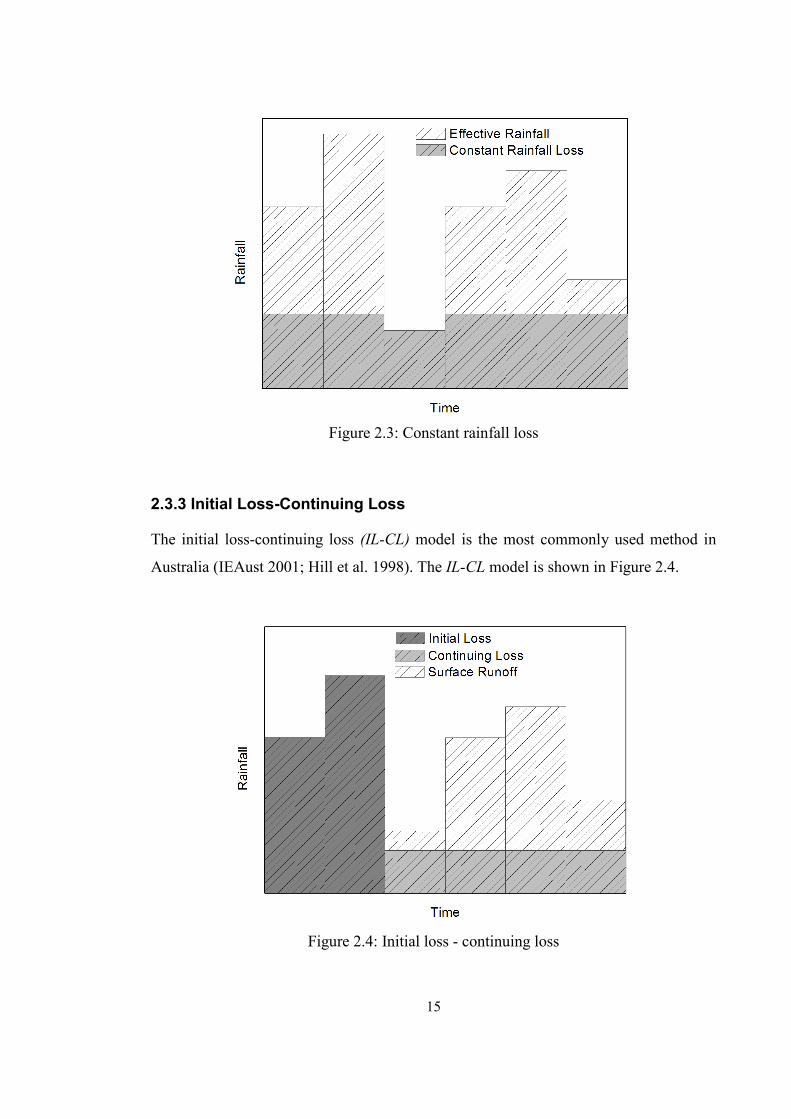
Figure 2.3: Constant rainfall loss

2.3.3 Initial Loss-Continuing Loss

The initial loss-continuing loss (IL-CL) model is the most commonly used method in

Australia (IEAust 2001; Hill et al. 1998). The IL-CL model is shown in Figure 2.4.

Figure 2.4: Initial loss - continuing loss

16

The method is similar to the constant loss rate except that there is no runoff assumed to

occur until a given initial loss (IL) capacity is satisfied, regardless of rainfall rate. At the

beginning of a storm event, IL starts prior to the commencement of any surface runoff,

and throughout the remainder of that storm continuing loss (CL) occurs, which is the

average rate of rainfall loss after the fulfilment of IL from surface runoff.

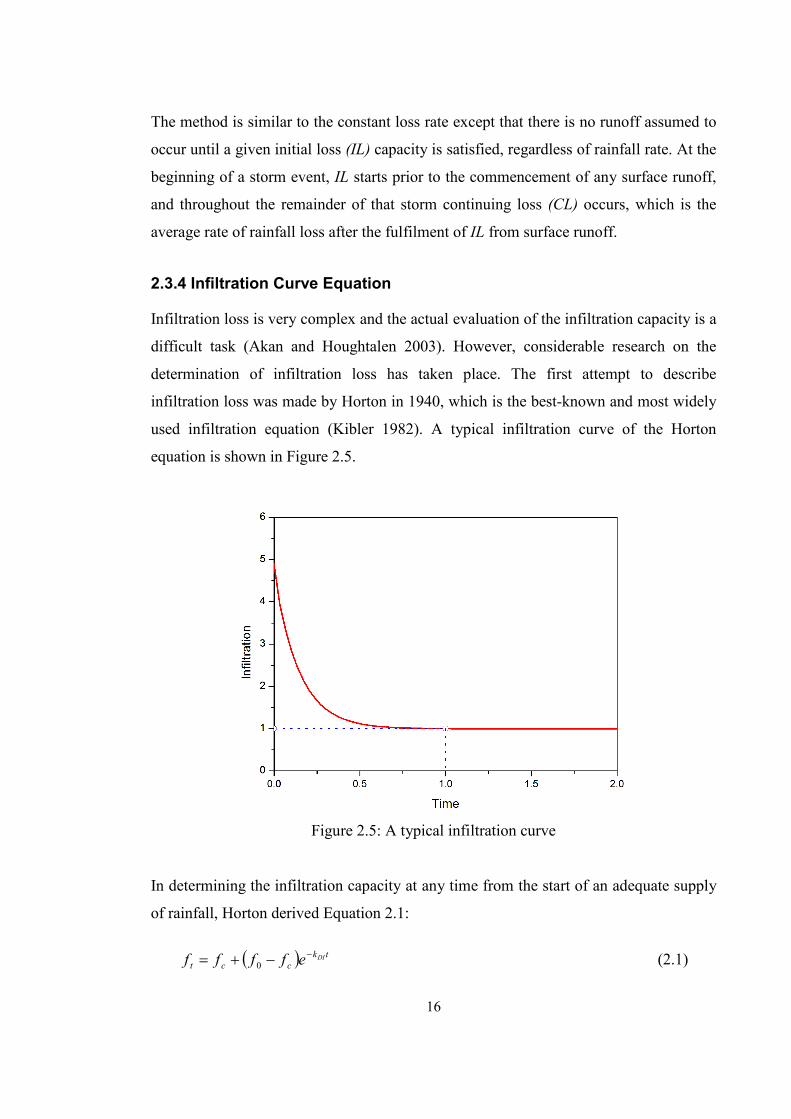
2.3.4 Infiltration Curve Equation

Infiltration loss is very complex and the actual evaluation of the infiltration capacity is a

difficult task (Akan and Houghtalen 2003). However, considerable research on the

determination of infiltration loss has taken place. The first attempt to describe

infiltration loss was made by Horton in 1940, which is the best-known and most widely

used infiltration equation (Kibler 1982). A typical infiltration curve of the Horton

equation is shown in Figure 2.5.

Figure 2.5: A typical infiltration curve

In determining the infiltration capacity at any time from the start of an adequate supply

of rainfall, Horton derived Equation 2.1:

( ) tkcct

DIeffff −−+= 0 (2.1)

17

Where, ft is the infiltration capacity (mm/hr) at time ‘t’, f0 is the initial infiltration

capacity (mm/hr), fc is the final or equilibrium or constant infiltration capacity (mm/hr)

and kDI is the exponential decay constant representing the rate of decrease in the

infiltration capacity.

Equation 2.1 is suitable for small catchments because the values of fc and kDI are

dependent on soil types and vegetation. Larger catchments tend to be heterogeneous,

and soil types and vegetation are not the same throughout an entire catchment (Ilahee

2005). In addition, difficulties in the determination of f0 and kDI restrict the use of

Equation 2.1 (Veissman and Lewis 2003).

2.3.5 Proportion Loss Rate

Proportion loss is considered to be a (constant) fraction of rainfall after surface runoff

has commenced. In this model, rainfall loss is assumed to be a fixed proportion of

rainfall as shown in Figure 2.6. In Australia, the model is used in conjunction with the

IL model (Ilahee 2005). However, for the widespread application of this model, further

investigation is needed.

Figure 2.6: Proportion loss

18

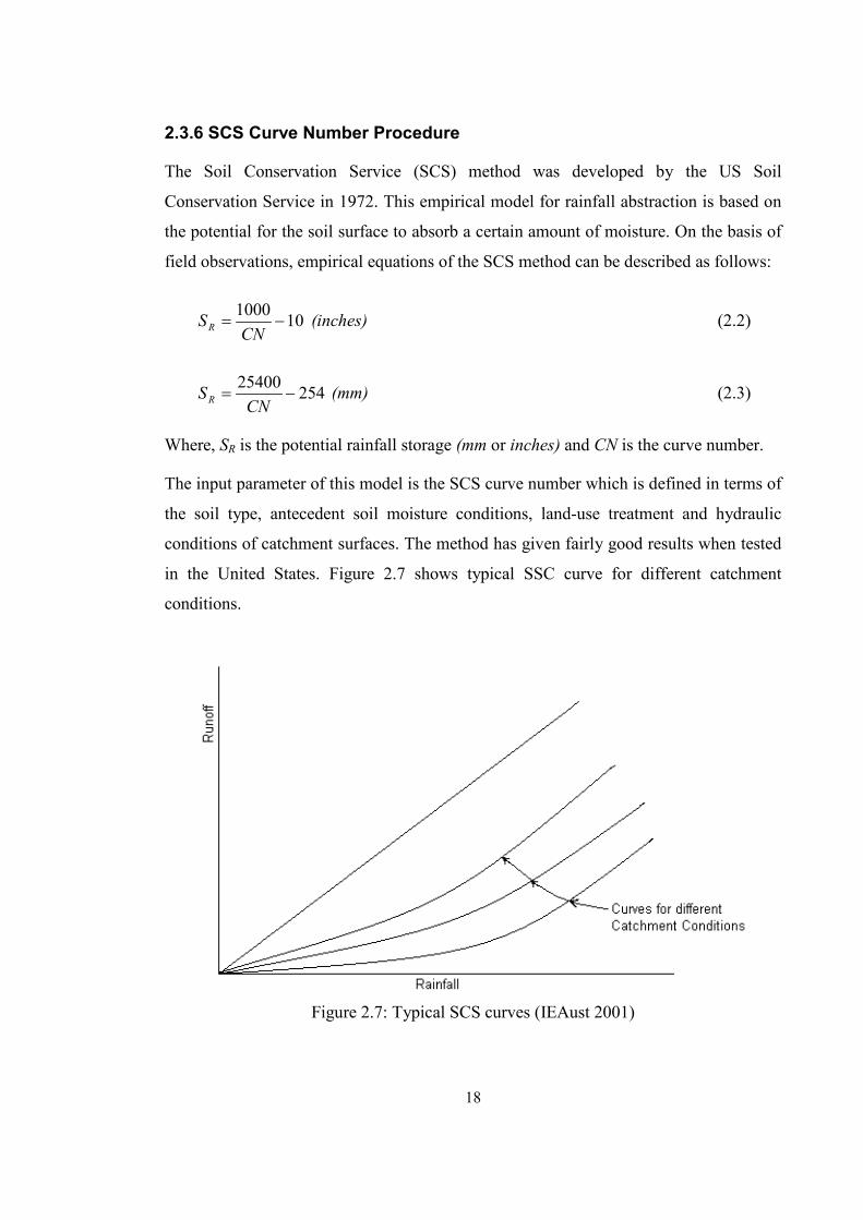
2.3.6 SCS Curve Number Procedure

The Soil Conservation Service (SCS) method was developed by the US Soil

Conservation Service in 1972. This empirical model for rainfall abstraction is based on

the potential for the soil surface to absorb a certain amount of moisture. On the basis of

field observations, empirical equations of the SCS method can be described as follows:

101000−=

CNSR (inches) (2.2)

25425400−=

CNSR (mm) (2.3)

Where, SR is the potential rainfall storage (mm or inches) and CN is the curve number.

The input parameter of this model is the SCS curve number which is defined in terms of

the soil type, antecedent soil moisture conditions, land-use treatment and hydraulic

conditions of catchment surfaces. The method has given fairly good results when tested

in the United States. Figure 2.7 shows typical SSC curve for different catchment

conditions.

Figure 2.7: Typical SCS curves (IEAust 2001)

19

2.4 Primary Water Quality Parameters Water quality parameters have the significant impact upon the quality of surrounding

environments and aquatic ecosystems. During the antecedent dry days (td) (i.e. the days

without rain), pollutant loads are accumulated on catchment surfaces. Throughout storm

events, rainfall encounters these contaminants from the time rainwater falls on the

ground surface to the time it reaches into receiving water bodies (Tsihrintzis and Hamid

1997). Moreover, rainwater can be polluted before it reaches to the ground surface

(Vazquez et al. 2003). It is difficult to prevent stormwater runoff from polluting

environments because surface runoff can be contaminated almost anywhere that rain

falls (CRC for Catchment Hydrology 2005). When surface runoff occurs, it washes

away and transports water quality parameters and soil sediment on its path till finally

they are discharged into receiving water bodies (Bannerman et al. 1993; Novotny et al.

1985; Sartor et al. 1974) and deteriorates the quality of surrounding environments.

Since stormwater pollution leads to the significant deterioration of surrounding

environments, identification of the specific characteristics and types of pollutants is

critically important. To address water quality concerns adequately with stormwater

runoff, it is important to understand types of pollutants which are present as well as their

potential impact into receiving water bodies (Adams and Papa 2000). The common

water quality parameters which deteriorate the quality of an aquatic environment are:

Litter

Suspended sediments/solids

Nutrients

Heavy metals

Hydrocarbons

Total organic carbon

2.4.1 Litter

Litter is the most obvious component of stormwater pollution. Over the last 30 years,

pollution of the environment from the export of litter has intensified due to the

production of easily disposable, non-biodegradable packaging materials, and

commercial and industrial items (Wong et al. 2000). Shaheen (1975) found that 20% of

the weight of pollutants which accumulate on road surfaces is litter.

20

Litter can be categorised as two types, i.e. artificial litter and natural litter. Packaging

materials (paper, glass, metal, plastics etc.) are artificial litter, which mainly originates

from construction or demolition activities. Litter originating from vegetative materials is

called natural litter. Most of the urban catchments produce a significantly high volume

and mass of litter.

The significance of litter as a water quality polluting agent is comparatively low.

However, litter contributes to the blockage of urban drains and causes the unsightly

appearance of receiving waters. During rainfall events, litter is washed-off from

catchment surfaces and drains into streams and creeks. They interfere with the quality of

water aesthetically and threaten animals, plants and fishes which live into waterways

and water bodies (MW-Web 2011). In addition, Rahman et al. (2002b) found that leaf

litter forms a significant component of SS in forested catchments.

2.4.2 Suspended Sediments/Solids

The term suspended sediment/solid (SS) is used to describe one of the major water

borne pollutants. It refers to the mass or concentration of inorganic and organic

materials suspended in water which is detached and transported (eroded) from their

original sites. It is well recognised that SS is the most prevalent component in the

deterioration of the quality of water, aquatic environments and their ecosystems.

Therefore, an in-depth knowledge of the SS characteristics in stormwater runoff is

critical. A clear understanding of SS especially particulate pollutants will aid watershed

management authorities developing strategies to reduce the export of pollutants to

surface water (Vaze and Chiew 2004).

A large portion of stormwater pollutants originating from a particular catchment surface

is particulate matters (Vaze and Chiew 2004). During a storm event, some of the

particulate matters are dissolved into rainwater. However, because of raindrop induced

energy, a significant amount of particulate pollutants are kept in suspension in the

overland flow (Shaw et al. 2010; Egodawatta et al. 2007) and transported to nearby

streams with surface runoff. Hence, the concentration of SS in stream water increases

during a storm event.

21

Excessive levels of SS in water bodies have the significant deleterious impact on

physical, chemical and biological properties of nearby waterways and receiving water

bodies (Bilotta and Brazier 2008). The physical alterations of water quality due to SS

are associated with the undesirable aesthetic effects of polluted water, the higher water

treatment costs, reduced navigational facilities of streams, and decreased longevity of

dams and reservoirs (Butcher et al. 1993). The deposition of SS can block pipes, change

in the flow conditions in open channels and disrupt habitats of aquatic invertebrates and

fishes (Duncan 1999). In addition, the deposition of sediment particles raises the stream

bed, lakes and ponds, reduces the discharge capacity of streams, impacts upon

navigational facilities; and hence causes floods during high rainfall events (Lawrence

and Atkinson 1998). The recreational uses of water, such as boating and swimming may

be reduced due to turbidity of water. Turbidity from SS also makes water cloudy or

muddy which leads to the reduction in light penetration through the water column,

temperature changes, and infilling of channels and reservoirs by their deposition.

Sedimentation problems of natural rivers arise from river management when there is an

inadequate prediction of the sediment behaviour (Ali et al. 2010).

The chemical alterations caused by SS into waterways and water bodies include release

of contaminants, such as heavy metals, pesticides and nutrients (Russel et al. 1998;

Miller 1997). Furthermore, SS with a high organic content undergoes anaerobic

breakdown and depletes the level of oxygen during their decomposition. This produces

a critical oxygen shortage, which can leads to fish kills during low-flow conditions

(Ryan 1991). Moreover, large amounts of bioorganic matters and heavy metals are

bounded to SS (Deletic 2001).

The biological effects of high level SS on different groups of organisms are different.

Increase in SS during a storm event can have the ecotoxic effects to aquatic organisms

(Rossi et al. 2006). The growth rate of photosynthetic organisms is reduced by the high

concentration of SS (Akan and Houghtalen 2003; Adams and Papa 2000; Duncan 1999).

Deposition of SS can clogs fish gills and reduces spawning, resulting in lower fish

populations or a shifting of fish species. Decline of fishery resources and serious

ecological degradation of an aquatic environment are the results of excessive SS

concentration.

22

Significant amounts of other pollutants are also transported as solid-bound contaminants

with surface runoff. Zoppou (2001) noted that some of the main water quality

parameters adhere to SS particles and conveyed along with soluble pollutants by surface

runoff. Zhou et al. (2003) found that SS are closely linked to environmental problems

due to the role of sediment particles in adsorbing and transporting contaminants. Vaze

and Chiew (2004) found that particulates of TP and TN in stormwater runoff are

attached to the sediment particles between 11 and 300 µm. Wong et al. (2000) found

significant amounts of inorganic pollutants in SS. Herngren et al. (2005); Akan and

Hougtalen (2003) and Sartor et al. (1974) found a strong correlation between SS and

heavy metals, nutrients and hydrocarbons. Sartor and Boyd (1972) reported that 50% of

heavy metals are adsorbed to the particle size less than 43 µm. They further found that

one third to one half of algal nutrients is attached to that sediment size. As the

correlation between SS and other pollutants are strong, the presence of SS in water

indicates the presence of other pollutants, such as heavy metals, nutrients.

2.4.3 Nutrients

Nutrients are chemical compounds that play important roles in all forms of life (Wong

et al. 2000). They are important to maintain the productivity of an agro-ecosystem.

Since these elements are essential to the life processes of aquatic organisms, they are

referred to as nutrients (Bowie et al. 1985). Without nutrients, a healthy ecosystem

cannot be considered. However, the presence of an excess concentration of nutrients

into water bodies is considered as pollution.

An excessive amount of nutrients in the water environment can cause the detrimental

effects to the health of an aquatic ecosystem (Wong et al. 2000). The increased

concentration of nutrients into surface waters accelerates the eutrophication process

(Laenen and Dunnette 1997). Eutrophication is the enrichment of water bodies with the

dissolved nutrients, which causes the depletion of available oxygen in water and

disturbs the biological equilibrium in water ecosystems. Eutrophication in surface water

(e.g. rivers, dams, lakes and estuaries) in combination with other physio-chemical

factors (i.e. increased water inflow from rainfall events and stratification) lead to the

enhanced aquatic plant growth which is often referred as algal bloom (Robson and

Hamilton 2003; Byun et al. 2005).

23

Algal bloom ultimately results in the de-oxygenation of water, reduces aesthetics and

increases toxicity and contributes to the loss of diversity to aquatic environments

(Drewry et al. 2006). The excessive growth of algae also alters the appearance of water

bodies affecting the colour, odour, turbidity and floating matter water. Decaying algae

cause undesirable odours and affects the taste of drinking water.

The major nutrients are nitrogen, phosphorus, carbon, calcium, potassium and silicon

(Bowie et al. 1985). There are also some other micronutrients, such as iron, manganese,

sulphur, zinc, copper, cobalt and molybdenum, which are essential for aquatic plants.

However, these micronutrients are usually present only in trace amounts and they meet

the biochemical requirements of organisms. For example, carbon is not considered to be

a limiting nutrient in an aquatic system. In most situations, carbon does not limit algal

growth; and hence the carbon simulation can be omitted in water quality modelling.

Silicon is a limiting nutrient only for diatoms. Therefore, the biogeochemical cycle of

silicon is generally modelled only when diatoms are simulated as a separate

phytoplankton group (Bowie et al. 1985).

From the water quality perspective, nutrients that play an important role in water quality

deterioration are: total nitrogen and total phosphorus (Ballo et al. 2009; Carpenter et al.

1998). Algal growth is typically limited by either of these two nutrients (Bowie et al.

1985). Total nitrogen (TN) is the sum of total kjeldahl nitrogen (TKN) and oxidised

nitrogen. On the other hand, TKN is comprised of organic nitrogen and ammonia

nitrogen; while oxidised nitrogen is comprised of nitrite nitrogen and nitrate nitrogen.

Both nitrite and nitrate in drinking water contribute to methemoglobinemia illness or

blue baby syndrome. Total phosphorus (TP) is the sum of the dissolved and particulate

phosphorus which can be sub-divided into reactive, acid-hydrolysable and organically

bound according to its chemical availability (Duncan 1999).

2.4.4 Heavy Metals

In a large number of water quality studies (e.g. Wong 2006; Adams and Papa 2000;

Sartor and Boyd 1972), the concentration of heavy metals were recorded. Depending

upon the prevailing redox and pH condition, heavy metals can be organic or inorganic

or complex and usually exist in a variety of ionic species (Ball et al. 2000).

24

The common heavy metals found in stormwater runoff in urban areas are: Zinc (Zn),

Lead (Pb), Copper (Cu), Cadmium (Cd), Mercury (Hg), Arsenic (As), Nickel (Ni) and

Chromium (Cr). The presence of heavy metals in stormwater runoff is of concern

because most of these metals are toxic to aquatic lives (Akan and Houghtalen 2003;

Davis et al. 2001; Ball et al. 2000). Environmental toxicity is depended largely on their

concentration in the solution. Unlike most other water borne pollutants, heavy meals

cannot be chemically destroyed or integrated into the environment (Davis et al. 2001).

They may be transported attached to sediments or in a soluble or dissolved form. Most

heavy metals are cumulatively accrued in an aquatic environment rather than the

instantaneous flux (Ball et al. 2000). They have a strong affinity to attach smaller

particle sizes due to the capacity of absorbing fine solids because of their relatively

larger surface area (Deletic and Orr 2005). The conventional pollutant removal

processes have little impact in reducing heavy metals from stormwater runoff

(Miguntanna 2009).

2.4.5 Hydrocarbons

Hydrocarbons are important water quality parameters especially in urban environments.

Generally, hydrocarbons refer to organic compounds which contain carbon and

hydrogen. The main types of hydrocarbons which degrade the quality of water are total

petroleum hydrocarbons (TPH) and polycyclic aromatic hydrocarbons (PAHs), which

form a sub-group within TPH (Miguntanna 2009).

Hydrocarbons are crucially important in water quality study because some of their

compounds are toxic to aquatic environments (Gobel et al. 2007; Akan and Houghtalen

2003). Herngren et al. (2005) found that there is a strong correlation between heavy

metals and hydrocarbons. Ball et al. (2000) noted that similar to heavy metals and

nutrients, hydrocarbons in stormwater runoff are mostly associated with the sediment

particles. According to Datry et al. (2003), most of the hydrocarbons are attached to

particulate matters. Wong (2006) found that many organic hydrocarbons can persist in

sediment for long periods and they are dangerous at very low concentration. As a result,

benthic organisms are particularly vulnerable to these organic toxicants. Therefore, an

increased concentration of hydrocarbons leads to increase the toxicity of waterways and

receiving water bodies (Polkowska et al. 2001).

25

2.4.6 Organic Carbon

Organic carbon is considered to be another major water quality parameter in urban

stormwater runoff. It reflects the level of natural organic substances or humic minerals

in water samples. Organic carbon is the measure of all carbon atoms covalently bonded

in organic molecules (Wong 2006).

The common impact of organic matter in water is the reduction in dissolved oxygen

(DO) due to microbial oxidation. Decomposition of organic matter depletes DO into

receiving water and affects aquatic environments (Akan and Houghtalen 2003). Hence,

excess organic carbon means excessive oxygen demanding materials into receiving

water and causes significant damage to aquatic lives (Warren et al. 2003). Moreover,

Lin and Chen (1998) found a positive linear relationship between organic matter and

heavy metals. Furthermore, a substantial level of organic matter leads to anaerobic

conditions resulting in fish kills, foul odours and discolouration. Organic carbon in

sediment solution leads to the solubility enhancement effect (Warren et al. 2003).

Solubility enhancement is the reduction of solid-solution partition coefficient which

reduces the total sediment sorbed amount, thereby increasing the soluble fraction

(Goonetilleke and Thomas 2003). In addition, Wu et al. (2004) noted that organic matter

is the main sorbent of hydrophobic pesticides in water systems.

2.4.7 Pathogens

Every stream contains some microorganisms many of which are harmless. However,

some of them can cause diseases to human which are called pathogens (MW-Web

2011). The common pathogens associated with the water quality degradation, include

bacteria, viruses and protozoa (Miguntanna 2009). They are disease causing organisms

and are sometimes responsible for epidemics. Pathogens cause some fatal waterborne

diseases, such as diarrhoea, dysentery, hepatitis, cholera or typhoid fever (Wong 2006).

Sources of pathogens in streams and creeks include human and animal faecal wastes

(MW-Web 2011). They enter via stormwater drains, sewer overflows, animals in

catchments, poorly maintained septic tanks, failing decentralised wastewater treatment

systems and illegal sanitary sewer cross-connections. Some of the pathogens (e.g.

enteric viruses) have the ability to replicate themselves within hosts (Herngren 2005).

26

2.5 Sources of Water Quality Parameters Water quality parameters can originate from a variety of sources on catchment surfaces.

Knowledge of the sources of pollutants allows decisions to be made to target the

reduction of pollutants and evaluating the changes in pollutant loadings due to the

modification in land-use and development. Proper knowledge of pollutant sources helps

to estimate the effects of water system configurations on contaminant flows and their

control. Bohemen and De Laak (2003) noted that the most effective way to control the

flow of water quality parameters is to control them at the source.

There are a range of natural factors (climate, topography, geomorphology, geology, soil

type and vegetation community type) as well as land-use and land management

practices which determine the quality of water (O’Reagain et al. 2005). However,

human activities are the prime reason for the accumulation of pollutant loads on

catchment surfaces (Hoorman et al. 2008).

Urban expansion and consequent anthropogenic activities, agricultural activities,

fertilizer applications, deterioration of forests, any physical changes on catchment

surfaces and other human activities alter the natural condition of an existing

environment. Due to these natural and anthropogenic sources, non-point pollutant loads

are accumulated during the antecedent dry periods. Failures in urban infrastructures,

such as sewer infiltration, leachate from landfills and direct connection of sanitary

sewers to stormwater drains also increase the accumulation of pollutant loads (CRC for

Catchment Hydrology 2005).

Most of the pollutants are either dissolve or otherwise transported with surface runoff

and eventually end up in receiving water bodies. Therefore, surface runoff from

different types of land-use is enriched with different types of pollutants. Hence,

stormwater runoff is considered to be the major problem into nearby waterways and

receiving water bodies. Different researchers have identified diverse sources of water

quality parameters which impacts upon the quality of an aquatic ecosystem. The

categories of important natural pollutants are geological, hydrological and climatic.

Usually, surface water is impaired by water quality parameters input from the both point

and non-point sources.

27

2.5.1 Point-source and Non-point Sources Pollutants

Pollutant loads coming from an identifiable source are called point source pollutants;

while pollutants coming from many unknown sources are called non-point source

pollutants. Point source pollutants can be predicted, controlled and reduced by imposing

regulations. However, the prediction of the non-point source pollutants are difficult; and

hence non-point source pollution, such as runoff from agricultural land, industrial and

highly urbanised areas have the profound impact on both surface runoff and

groundwater (Deletic 2001). Today, after years of extensive research in this area, it is

clear that non-point source pollution (also called diffuse source pollution) is a

significant problem to surrounding water environments (Novotny and Olem 1994). The

common non-point source pollutants are categorised as sediments, nutrients and sewage.

They can be originated from (Goonetilleke and Thomas 2003):

transportation activities

industrial/commercial activities

construction and demolition activities

corrosion of materials

vegetation

soil erosion

atmospheric fallout

spills

2.5.2 Transportation Activities

Transportation activities are considered to be one of the major contributing sources of

water quality parameters. According to Puckett (1995), 38% of the atmospheric nitrogen

emission may come from transport activities. Transport related pollutants are mainly

generated on street surfaces. Therefore, street surfaces are considered to have the

profound impact on water quality parameters which are mainly generated from vehicles.

Although highways and freeways represent only a minor portion of catchment

imperviousness, they are significant sources of water quality pollution (Wong et al.

2000). A summary of the sources of street surface contaminants, which are directly

related to anthropogenic and traffic related activities is presented in Table 2.1.

28

Table 2.1: Typical road runoff contaminants and their sources (Ball et al. 1998)

Contaminants Primary source

Sediment Pavement wear, vehicles, atmosphere, maintenance activities

TN, TP Atmosphere, roadside fertiliser applications

Lead Auto exhaust, tyre and bearing wear, lubricating oil and grease

Zinc Tyre wear, motor oil, grease

Iron Automobile rust, highway steel structures (e.g. guard rails),

moving engine parts

Copper Metal plating, bearing and brush wear, moving engine parts,

brake lining wear, fungicides, insecticides, pesticides

Cadmium Tyre wear, insecticide application

Chromium Metal plating, moving parts, brake lining wear

Nickel Diesel fuel and petrol exhaust, lubricating oil, metal plating,

brush wear, brake lining wear, asphalt paving

Manganese Moving engine parts, automobile exhaust

Cyanide Deicing compounds

Sodium/Calcium

Chloride

Deicing salts

Sulphate Roadway surfaces, fuels, deicing salts

Petroleum

hydrocarbons

Spill, leakages or blow-by of motor lubricants, anti-freeze and

hydraulic fluids, asphalt surface leachate

Polychlorinated

biphenyls (PCB)

Background atmospheric deposition, PCB catalysts in synthetic

tyres, spraying of right-of-way

PAHs Asphalt surface leachate

Numerous research studies have identified street surfaces as significant contributors of

water quality parameters (Egodawatta and Goonetilleke 2008; Zafra et al. 2008;

Drapper et al. 2000; Bannerman et al. 1993; Sartor and Boyd 1972). Hoffman et al.

(1985) found that over 50% of the total annual pollutants input of SS, polycyclic

aromatic hydrocarbons and heavy metals of the Pawtuxet River, USA originated from

street surfaces. This is due to the direct and continuous anthropogenic activities on street

surfaces.

29

However, the accumulation of water quality parameters on street surfaces varies widely

depending on a wide range of factors. Gobel et al. (2007) noted that the concentration of

pollutants from street surfaces vary with the traffic density, wind drift, duration and

intensity of stormwater events, the duration of dry weather periods and the state of the

traffic technology. Sartor and Boyd (1972) identified pavement conditions and

pavement materials as important sources of water quality parameters on street surfaces.

They also found that asphalt pavements contribute 80% more pollutant loadings than

concrete surfaces. Furthermore, the accumulation of water quality parameters on a street

surface depends on the location of traffic lights, road layout, pavement surface

roughness and driver’s habits (Goonetilleke and Thomas 2003).

2.5.3 Industrial/Commercial Activities

Industrial and commercial activities have the reflective impact on the accumulation of a

wide range of water quality parameters on catchment surfaces. Due to the wide range of

industrial activities and chemical use heavy metals are especially found in the urban

areas. Numerous researchers identified different categories of water quality parameters

in industrial and commercial areas. For example, the studies of Ghafouri and Swain

(2004); Lau and Stenstrom (2005) and Brezonik and Stadelmann (2002) found that

industrial and commercial areas have the relatively high concentration of water quality

pollutants compared to other land-uses. Sartor and Boyd (1972) found that the

accumulation of TP in a catchment surface was 14.3 g/m2 for commercial areas and 51.8

g/m2 for industrial areas. In addition, Bannermann et al. (1993) found that streets and

parking lots are the critical source areas for the generation of water pollutants in

industrial and commercial areas.

The major water quality parameters from various industrial/commercial activities

contain a significant amount of nutrients, heavy metals and chemical toxins (Lee and

Bang 2000). In addition, hydrocarbons, dust and other chemicals are also related to

these activities (US EPA 1993). The industrial sources of pollutants are exposed

storage, loading and unloading, equipment, spills and leaks, industrial materials and

waste products (Miguntanna 2009). Water quality parameters in commercial areas are

generated mainly from motor fluids from parked cars, large parking lots, auto service

stations, gas stations, shopping centres and restaurants.

30

Sartor and Boyd (1972) found the highest metal concentration in road sweepings from

industrial areas. Kelly et al. (1996) noted that due to the extensive burning of fossil fuel,

heavy metals are accumulated in industrial areas. In addition, Herngren et al. (2006)

found the highest heavy metal loadings coincided with areas of the highest sediment

loadings which occurred in commercial areas. Latimer et al. (1990) found that

particulate pollutants in industrial sites have the highest concentration of hydrocarbons.

Armitage and Rooseboom (2000) noted that industrial and commercial activities

significantly influence the accumulation of litter. Puckett (1995) found that 53% of the

atmospheric deposited nitrogen in the north-eastern states in the US came from large

industries, such as coal and oil burning, and electric utilities. Therefore, areas with

industrial or commercial activities are considered to be one of the most significant

sources of water quality parameters (Pitt et al. 1995).

2.5.4 Construction and Demolition Activities

Construction and demolition activities have the potential to contribute a significant

amount of water quality parameters. In urban areas, construction activities are the most

hazardous for sediment generation (Jartun et al. 2008). During a relatively short period,

construction sites can contribute more solids into receiving water bodies than that can

be deposited naturally over several decades (Miguntanna 2009). This is primarily

attributed due to the higher soil erosion from construction sites.

Construction activities contribute most sediment on a unit area basis of a particular

catchment (Nelson and Booth 2002). After investigating different land-uses in the USA,

Line et al. (2002) found that the highest sediment export rate came from a construction

site which was 10 times more than from other sites. They also found the highest amount

of annual TN export from construction sites. In addition, Sonzogni et al. (1980) noted

that urban construction sites contribute more phosphorus than any other land-use.

Wind transports on-site pollutants from construction sites which are then accumulated

on roofs, front yards and roads. High traffic volume close to construction and

demolition activities forces pollutants to be accumulated on curbs (Brinkmann 1985).

However, pollutant loads vary considerably with the amount of construction, catchment

area, management of the site and maintenance activities (Miguntanna 2009).

31

2.5.5 Vegetation

Stormwater runoff contains not only inorganic pollutants but also organic vegetative

pollutants. Waste vegetative matter from tree leaves and other plant materials, such as

pollen, bark, twigs and grass are potential contributors of both organic pollutants and

nutrients as they break down in catchments and in waterways. Line et al. (1997) found a

significant amount of nutrients where a large amount of organic waste was present.

They further noted that the concentration of TKN is increased during the periods of

pollen deposition. Novotny et al. (1985) noted that a mature tree can produce 15 to 25

kg of organic leaf residues which contain a significant amount of nutrients. In addition,

Dorney (1986) found that TP in urban street leaves are similar to TP from trees in

natural ecosystems. Therefore, Cowen and Lee (1973) emphasised on the leaf pickup to

minimise phosphorus content in urban drainages runoff.

However, Allison et al. (1998) have questioned the importance of leaf litter as a

potential source of nutrients in urban stormwater. They found that potential nutrients

contribution from the leaf litter is two orders of magnitude smaller than the measured

total nutrient loads. Their findings were based on the outcomes of an urban catchment

located in an inner city suburb of south-east Australia. Their observations confirm that

water quality pollutants are dictated by the site-specific factors.

2.5.6 Soil Erosion

Soil erosion is the major contributor of SS in stormwater runoff. Nelson and Booth

(2002) noted that the ubiquitous source of SS is the erosion of landscape areas either

from natural or anthropogenic activities. Erosion starts with the impact of a raindrop,

which can vary from 1/16 inch to 1/4 inch in diameter with maximum speed of 20 mph

at the ground surface. The subsequent collisions between raindrops and the earth surface

break the soil particles into their components (sand, silt, and clay). Surface runoff

transports these smaller particles of silt and clay to the downstream. The force of

flowing water also detaches the soil particles and transports them into receiving water

bodies. The adsorbed pollutants with soil particles settle in the stream bed and in flood

plains which causes physical, chemical and biological harm into receiving water bodies

(US EPA 1993).

32

The most common factors affecting erosion of soil include the intensity and duration of

rainfall, frequency of storm, snow cover and antecedent rainfall (Sonzogni et al. 1980).

Soil types, topography, vegetation and climatic conditions also have a significant

influence on soil erosion. Any land practice that exposes soil to erosive forces of rainfall

and runoff represent erosion and pollutant hazards. During the active construction

period, protective vegetative cover is removed from construction sites and the

unprotected soil is left exposed to rainfall (USGS 2000). The loss of vegetative cover

from the ground surface allows raindrops to strike with its full energy, which increases

soil erosion and leads to increase the concentration of SS into stormwater runoff.

Additionally, stream bank erosion increases the annual solid loads in an urbanised

catchment (Nelson and Booth 2002).

2.5.7 Corrosion of Materials

In areas where metal roofs dominate, corrosion is a significant source of water quality

pollution. Different metal elements, for example, Copper (Cu), Zinc (Zn), Aluminium

(Al), Lead (Pb) and other materials are used as roof coverings, gutters and down pipes.

All these materials release heavy metals in stormwater runoff as a corrosion product

(Gobel et al. 2007). Forster (1996) also found that the areas having appreciable

coverage of metal roofs are more liable to have the accumulation of heavy metals on

catchment surfaces. Similar results were obtained by Davis et al. (2001) in a

comprehensive study of urban water quality parameter sources. Their study was based

on a variety of building sides and roofs among other surfaces. Further study undertaken

by Bannerman et al. (1993) and Pitt et al. (1995) demonstrated that runoff from a

galvanised roof surface contains higher heavy metals concentration than runoff from

street surfaces.

Acid rain and aggressive gases contribute to a significant corrosion of roofs, gutters,

paints and other metal surfaces (Brinkmann 1985). Due to the low pH value of

rainwater, the corrosion process is enhanced (Gobel et al. 2007). During storm events,

the corroded particles are transported with surface runoff into waterways and receiving

water bodies. However, the amount of corroded pollutants on surface runoff depends on

many factors.

33

Brinkmann (1985) identified the most common factors responsible for the corrosion of

metal surfaces:

availability of corrodible materials

the frequency and intensity of exposure to an aggressive environment

the drying-rewetting frequency of the exposed surface

the character and the structure of materials

maintenance practices

2.5.8 Atmospheric Fallout

In certain regions, atmospheric deposition is recognised as a significant non-point

source of water pollution. Pollutants from atmospheric fallout include fine particulate

materials, sulphur and nitrous oxides, PAHs etc. (Bohemen and De Laak 2003).

According to Hoffman et al. (1984), most of the PAHs in the estuarine and coastal

sediments originate from atmospheric fallout. Airborne pollutants are deposited on the

earth surface and worsen the quality of water and water environments (Polkowska et al.

2001). Wang and Li (2009) found that the main contribution to the accumulation of

pollutants on a roof surface is atmospheric dry deposition rather than roof materials.

The sources of atmospheric deposition include industry, traffic, refineries, power plants

and waste processing companies (Bohemen and De Laak 2003). Emissions from

vehicles initially contribute to pollution of atmospheric environments but return to the

earth surface due to atmospheric deposition and they pollute stormwater runoff. Puckett

(1995) noted that the atmospheric nitrogen is one of the important sources of nutrients.

Davis et al. (2001) found that a significant amount of heavy metals from roof surface

runoff came from atmospheric deposition.

Deposition of atmospheric pollutants occurs in two ways, i.e. dry deposition and wet

deposition (Ball et al. 2000). Dry deposition is the direct transfer of dust, aerosol and

gas from the atmosphere to the earth surface; and wet deposition is due to rain, snow,

fog, dew and frost which contain substances leached-out from the atmosphere (Gobel et

al. 2007). These two methods of deposition are the most important sources of water

quality pollution (Brinkmann 1985).

34

2.5.9 Spills

This category of pollutants is difficult to define quantitatively either in terms of volume

or composition (Goonetilleke and Thomas 2003); and it is even difficult to predict the

occurrence of spills accurately. However, spills are concentrated in parking lots and

near traffic lights. The major source of spills is vehicular transport. Leakages of fuel,

motor oils and lubricants occur everywhere on road surfaces (Brinkmann 1985). In

addition, Sartor and Boyd (1972) noted that vehicular transports, building constructions

and industrial activities are considerable sources of spills. The adverse impact of spills

on water quality is reduced through good maintenance and management practices.

2.6 Roles of Mathematical Models Modelling is a commonly used tool in research and management of environmental

systems. The ability to use a mathematical model to simulate the behaviour of a system

has allowed environmental researchers and managers to predict how different scenarios

and stimuli affect various environmental systems. The complex relationships between

waste loads from different sources (point or non-point) and the resulting water quality

responses of receiving water bodies are best described with mathematical models

(Deksissa et al. 2004). Therefore, there exists a wide range of water quality models to be

used in managing water quantity and quality with respect to a variety of environmental

impacts. These models can predict physical, chemical and biological processes

occurring during transportation of water quality parameters (Perk 2006). According to

Perk (2006), the purposes of water quality models development and applications are:

to forecast travel time of pollutants

to assess the past, present, or future human exposure to pollutants

to predict the future conditions under various scenarios of the environmental

changes and management strategies, which are relevant to support decisions in

policymaking processes

to evaluate the effectiveness of possible management actions

to reduce water quality monitoring costs by replacing or supplementing

expensive measurements by cheaper model predictions

to gain improved understanding of mechanisms, which control pollutant

processes especially related to research and developing settings

35

2.7 Water Quality Modelling Approaches Since 1970 a number of water quality models have been developed for the simulation of

different water quality parameters of catchments and streams. Some of these models

were developed specifically for and individual area and geographic conditions. Each of

the models was developed in a unique way with the simulation characteristics and

properties that influence how its output should be interpreted. These models vary in

terms of their complexity, considered approaches, the personnel and computational

requirements, and data requirements for calibration and validation (Merritt et al. 2003;

Charbeneau and Barrett 1998). In addition, Radwan et al. (2003) and Zoppou (2001)

noted that the essential difference in modelling approaches is the information that can

be obtained from models, the sophistication of the analysis performed and the

simulation period.

Modelling approaches start from the very simple conceptual type to the complex data

intensive models. The simple models are unable to determine the controlling processes

of pollutants because they do not employ a sufficient number of processes (Cox 2003).

However, data requirements of the complex models prohibit their broader applications

to the practical problems (Eatherall et al. 1998). In addition, more complex models need

more computation effort and more data resources (Phillips and Yu 2001; Zoppou 2001;

Goonetilleke 1998). Snowling and Kramer (2001) also noted that complex models are

generally very sensitive and therefore it is difficult to predict water quality parameters.

The financial costs of a complex model further enhance the difficulty of their wider

application.

According to Lindenschmidt (2006), the most complex model is not necessarily the

most accurate. Increasing model complexity increases the number of degree of freedom

(i.e. more parameters and variables) which increases model sensitivity. Therefore, over-

parameterisation makes the calibration procedure difficult and reduces the predictive

capability of models. The users often try to use the simple models rather than the

complex ones because they are easier to calibrate and therefore reliable (Pearl 1978).

However, oversimplification of the catchments and pollutants behaviour may leads to

gross errors. On the other hand, the processes of different model parameters are

interrelated to each other, and hence increase the difficulty in pollutants prediction.

36

Snowling and Kramer (2001) demonstrated a hypothetical relationship among model

sensitivity, error and complexity. According to them, model sensitivity increases with

increasing model complexity due to the large number of parameters and their

interactions with state variables. However, more complex models are able to better

simulate the reality with more processes included and fewer simplifying assumptions;

and hence modelling error decreases. For any system, consequences of choosing a

model for a given complexity are illustrated in Figure 2.8. If a model is too complex, the

sensitivity will be large (too far to the right), and if a model is not complex enough, the

error will be large (too far to the left) as shown in Figure 2.8.

Figure 2.8: Model complexity, error and sensitivity relationship

(Snowling and Kramer 2001)

Depending upon the physical processes, model algorithms describing these processes

and data requirements, models fall into three main categories (Merritt et al. 2003):

Empirical or statistical/deterministic model

Conceptual model

Physics-based model

There are also other types of mathematical models, which fall within any of the three

categories.

37

2.7.1 Empirical Model

The empirical model type is generally the simplest of all modelling types. This type of

model is developed based on the general observation data. The computational effort and

data requirements for such models are usually less than for conceptual and physics-

based models (Merritt et al. 2003). The parameters of the empirical model are obtained

by the calibration procedure from the observed data. However, the empirical model type

is criticised for employing unrealistic assumptions of the physics. The advantage of the

empirical model is that it can be frequently used in complex models, as it can be

implemented in situations with the limited data and parameter inputs.

2.7.2 Conceptual Model

The conceptual model type is developed by incorporating underlying transfer

mechanisms and their dynamic behaviour. Any model developed based on Darcy’s or

Newton’s law is considered to be a conceptual model. The parameters of a conceptual

model are usually derived by the calibration procedure against the observed data, such

as stream discharge and concentration measurements. Therefore, this type of models

tends to suffer from problems of identifying their parameter values. Furthermore, like

the empirical model type, the parameters of the conceptual model have limited physical

interpretability due to the lack of the unique value. However, simpler conceptual models

have fewer problems than more complex models (Merritt et al. 2003).

2.7.3 Physics based Model

The physics-based model involves sophisticated approaches and solutions, which are

based on the fundamental physical equations. This model type is developed based on the

known sciences to simulate the processes on the basis of systems. The standard

equations used in such models are the conservation of mass and momentum for flow

and the conservation of mass for sediment (Merritt et al. 2003). Theoretically, the

parameters of this model are measurable and so are known. However, in practice, due to

a large number of factors involved, these parameters are often calibrated against the

observed data (Merritt et al. 2003). Nevertheless, there are too many parameters to be

quantified, i.e. they tend to be affected by over-parameterisation.

38

The derivation of mathematical expressions describing individual processes in the

physics based model is subject to numerous assumptions that may not be relevant in

many real world situations. The governing processes of the physics-based model are

derived at small scale and under very specific physical conditions; and hence this type

of model is useful for the short term simulation (Redwan et al. 2003).

2.7.4 Lumped and Distributed Models

Models can be considered as lumped or distributed based on applied areas. Models

developed without considering the spatial variability are lumped models; while models

reflecting the spatial variability of the processes are called distributed models. Most of

the urban runoff models are deterministically distributed (Nix 1994). The distributed

approach is also applicable to sediment transport modelling (Merritt et al. 2003).

However, data requirements of the distributed models are larger compared with the

lumped model. If the estimation at the catchment outlet is sufficient, then the lumped

model is sufficient. The choice of the lumped model or distributed model depends on

the desired output and the nature of management interactions.

2.7.5 Event Based and Continuous Models

In terms of the rainfall-runoff simulation, models can be categorised as event based

model and continuous model. The model used for the simulation of an individual storm

event is called event based model (Alley and Smith 1981); while the model developed

for the simulation of a catchment’s overall water balance for a long period is continuous

model. Continuous models are more advantageous than event based models (Tan et al.

2005; Boughton and Droop 2003). However, for the design of stormwater

infrastructures, event driven models are more appropriate (Zoppou 2001).

2.7.6 Deterministic and Stochastic Models

Depending upon the nature of the prediction, models can be divided into two types, i.e.

deterministic model and stochastic model. Deterministic model usually attempts to

simulate the actual physical process associated with runoff quantity and quality; while

stochastic model focuses on the probabilistic nature of pollutant processes (Barbe et al.

1996).

39

If any of the model variables is regarded as random variable having a probability

distribution, then the model is called stochastic. Otherwise, the model is deterministic.

For the same input, a deterministic model will produce the identical results (Zoppou

2001). However, a stochastic model will always produce different model responses as

one or more variables are selected from the random distribution.

2.8 Model Selection Although various modelling techniques are well developed, the distinction between

models is not well-defined (Zoppou 2001). Kronvang et al. (2009) presented the

ensemble modelling results of nutrients loads for 17 European catchments. They could

not find any single model to perform the best across all of the catchments. Each of the

model types serves a specific purpose and a particular model type cannot be

recommended as appropriate for all the situations. Models are likely to contain a mix of

modules from each model category. For example, while the rainfall-runoff component

of a water quality model may be the physics-based or conceptual, empirical

relationships are used to model the pollutant processes.

The ultimate decision for each modelling exercise depends upon the needs of the users

and the purpose of modelling endeavour (Snowling and Kramer 2001). However, model

should be easily applicable and usable for planning and management by water

authorities (Laenen and Dunnette 1997). The choice of appropriate model depends on

many factors. Tan et al. (2005) identified two main factors that define model selection,

i.e. the objectives of the study and the availability of data and resources. According to

Merritt et al. (2003), for the practical application, selection of the most appropriate

model requires the consideration of the following factors:

the intended use and objectives of the model users

suitability of the model to the local conditions

data requirements of the model, including spatial and temporal variation of the

model inputs and the output

complexity of the model structure

various components of the model structure

the capability of the model including the accuracy, validity and underlying

assumptions

40

In addition, Akan and Houghtalen (2003) identified some important factors which affect

the choice of a particular model for a practical application:

the model is widely accepted (by engineers, consultants and regulators)

the model is inexpensive (written for personal computers with good user

support)

the model is user friendly (preferably using Windows environment)

the model is flexible and robust

the model is technologically advanced

2.9 Hydrologic Modelling Approaches The evaluation of hydrologically induced mobilisation of water quality parameters from

watershed areas has received considerable attention in the recent hydrological modelling

studies (Rusjan et al. 2008; Withers and Jarvie 2008). Hydrologic modelling is the

technique which is used to estimate the quantity of runoff from a particular catchment

area after a successive rainfall event. Hydrologic models were first developed for

natural or rural catchments. With the increasing demand for urban hydrologic models,

these types of models are modified to handle the urban characteristics (Ahyerre et al.

1998). At present, the same hydrologic model is used for both rural and urban

catchments or partly rural and partly urban.

It is widely recognised that if runoff cannot be estimated accurately, pollutant loads

cannot be predicted reliably. This is due to the two reasons. Firstly, pollutant loads

cannot be determined without having the estimated flows. Hence, hydrological models

form the basis of water quality models (White 1989). Secondly, the procedures to

mitigate water quantity and quality are often complementary. Therefore, most of the

water quality models are developed based on watershed hydrology or closely related to

simulate diffuse pollutant loadings (Novotny and Olem 1994).

Over recent years, a large number of hydrologic models (RORB, XP RAFTS etc.) were

developed to compute catchment runoff only. However, there are a number of models

(e.g. SWMM, MUSIC) which were developed to estimate both water quantity and

quality. Most of the models are based on the empirical relationships among drainage

area, time of concentration (tc), rainfall and other factors. They start from the very

simple which calculate only the peak discharge, to the complex which are capable of

41

estimating runoff hydrographs. However, all of the developed models cannot simulate

the continuous generation of surface runoff from catchment surfaces. Most of the

models developed are based on the event based simulation and they can simulate a

hydrograph for a single rainfall event only. The main types of hydrological modelling

procedures described in many hydrologic texts and in manuals (such as Australian

Rainfall Runoff) are as follows:

Rational method

Unit hydrograph method

Time-area routing method

Kinematic wave routing

Artificial storage routing

2.9.1 Rational Method

The first and most enduring hydrological method for the calculation of storm runoff is

the rational method (Gribbin 2007). The rational formula is the simplest form of

hydrologic model to estimate the peak discharge from a small watershed area. The

method was developed by Kuichling in 1889 for the measurement of discharges of

small drainage basins in urban areas. Since then it has become the most widely used

method for the design of small rural and urban watersheds structures (Viessman and

Lewis 2003).

For the design of very small hydraulic structures, derivation of a complete runoff

hydrograph is time consuming and becomes expensive. Only the peak discharge is

sufficient enough for the design of such structures. For these cases, the rational method

is very effective. The major advantage of the rational method is its simplicity.

Moreover, the method requires comparatively less data and resources to perform

calculations. The method is suitable for small (<25 km2) to medium (<100 km2)

catchments where there are limited data.

The rationale of this method is based on the concept that steady, uniform rainfall

intensity causes surface runoff at its maximum rate when all parts of a watershed area

are contributing to flow at a point of interest (Viessman and Lewis 2003). However,

there are certain assumptions which limit the use of the methods.

42

Dayaratne (2000) identified the fundamental assumptions adopted in the ration method

which can be described as follows:

rainfall is uniform all over a watershed area for the same period of time

the duration of rainfall is equal to the time of concentration

the peak flow is a fraction of overall rainfall rather than rainfall excess

rainfall-runoff response is linear

Mathematical expression of the rational method can be written as follows:

TyyuP AICCQ = (2.4)

Where, Qp is the peak discharge of a watershed area (L3/T), Cu is the unit conversion

coefficient, Cy is the dimensionless runoff coefficient corresponding to the return period

‘y’, Iy is the average rainfall intensity (L/T) for a storm with the return period ‘y’ and

storm duration tc, and AT is the total area of watershed (L2).

Although the formula is widely used, care should be taken in selecting the appropriate

runoff coefficient. The specific limitations of the method are as follows:

the method is capable of estimating only the peak discharge

the choice of the runoff coefficient is difficult

uniform rainfall is rarely experienced over an entire catchment

return period of both rainfall and runoff would rarely agree

the catchment tc many not be known

applicable to small catchments only

2.9.2 Unit Hydrograph

The concept of the unit hydrograph was first introduced by L.K. Sherman in 1932

(Gribbin 2007). The unit hydrograph of a watershed area is defined as the direct runoff

hydrograph resulting from one unit volume of excess rainfall of constant intensity and

uniformly distributed over a particular drainage area. A flood hydrograph can be

derived from a given rainfall excess hyetograph using the models developed based on

the unit hydrograph method. The unit hydrograph is catchment responses for a unit of

excess rainfall. The exact shape of the unit hydrograph depends on the characteristics of

a particular watershed area being considered.

43

Basic assumptions considered in the use of the unit hydrograph include the followings:

the effective rainfall has a constant intensity within the effective duration

the effective rainfall is uniformly distributed over a particular watershed area

the time base of a direct runoff hydrograph resulting from an excess rainfall of a

given duration is constant

ordinates of all direct runoff hydrographs of a common time base are directly

proportional to the total amount of direct runoff

For a particular watershed area, if the generalised pattern of a rainfall event is known, a

unit hydrograph is constructed for that area. Once the unit hydrograph is constructed,

then the total runoff hydrograph can be estimated for any rainfall amount by multiplying

the number of unit rainfall excess by the unit hydrograph. The superposition principle is

used to construct the total hydrograph for a rainfall event greater than the unit rainfall.

To do so, the rainfall excess is divided into a number of components, each equal to the

unit rainfall. Since each unit rainfall excess produces a unit hydrograph, all of the unit

hydrographs are combined to estimate the total hydrograph for that rainfall event.

Figure 2.9 shows the construction of a resultant hydrograph from two unit rainfall

events which occurred one after the other. Each of the unit rainfall produces a unit

hydrograph of equal magnitude.

Figure 2.9: Unit hydrograph constructed from multiple units of rainfall

44

However, the second unit hydrograph shown in Figure 2.9 is separated by a time value

equal to the unit time. The total hydrograph is constructed by plotting each of its

ordinates as the sum of ordinates of the two unit hydrographs at each point along the

time axis. In this way, the total runoff hydrograph is developed for any rainfall pattern

longer than the unit time.

2.9.3 Time-area Method

The time-area (TA) method of rainfall-runoff transformation is one of the most widely

used and suitable methods of hydrologic watershed routing (Shokoohi 2008; Saghafian

and Shokoohi 2006; Ponce 1989). During a rainfall event, the entire area of a catchment

is not contributing to surface runoff at the same time. The point close to the catchment

outlet contributes to surface runoff almost immediately after rainfall. After that the

contributing area increases which leads to an increase in surface runoff. Runoff

contribution from upstream parts of a watershed arrives at the later time, adding to the

contributing runoff from nearer points until flow arrives from all points of the watershed

(Viessman and Lewis 2003). Therefore, in watershed modelling, to account partial area

contribution of surface runoff, the TA method was developed.

The TA method was developed in the 1940’s (Shokoohi 2008). The method utilises a

convolution of rainfall excess hyetograph with a time-area histogram (TAH)

representing the progressive area contributions within a catchment in set time

increments (Ponce 1989). The method was developed without considering the storage

effects. In the TA method, the entire area of a catchment is deemed to contribute surface

runoff after the tc which is the time taken for a drop of water to reach at the outlet from

the furthest point of a particular catchment. A detailed description of the method can be

found in any hydrological hand book, such as Viessman and Lewis (2003). The

following is a short description of the method.

Figure 2.10 shows a catchment area which is divided into five sub-areas A1, A2, A3, A4

and A5. A rainfall event of the six different intensities shown in Figure 2.11(a) occurs

over the catchment. The time taken for surface runoff to reach from one sub-area to

another is Δt. At the beginning of a rainfall event, no part of the catchment contributes

to surface runoff and the initial flow Q0 is zero.

45

Figure 2.10: Catchment sub-area division

Figure 2.11: Rainfall and runoff contributed sub-areas

After the first time step Δt, only the sub-area A1 is contributing surface runoff to the

outlet. Thus the flow rate at the end of the first time step is calculated by Q1 = A1(RE)1.

Where, (RE)1 is the average rainfall excess for the first time step. At the end of the

second time step 2Δt, sub-areas A1 and A2 both are contributing flow to the catchment

outlet and the runoff rate is calculated by Q2 = A1(RE)2 + A2(RE)1. Where, (RE)2 is the

average rainfall excess for the second time step. Similarly, at the end of the third time

step 3Δt, sub-areas A1, A2 and A3 contribute to surface runoff and the flow rate is

determined by Q3 = A1(RE)3 + A2(RE)2 + A3(RE)1. Where, (RE)3 is the average rainfall

excess for the third time step. After the tc, all of the sub-areas contribute to surface

runoff. In this way the process continues until rain stops.

46

In the TA method, catchment shape is reflected in the TAH and runoff hydrograph. The

method can account for the temporal variation of rainfall intensity. In this method, the

unrealistic assumption made in the rational method of uniform rainfall intensity over an

entire catchment area during the tc is avoided. However, for very short rainfall events, it

produces erroneous results (Saghafian and Shokoohi 2006). Furthermore, the success of

the TA method mainly depends on the precision of isochrones mapping. Isochrones are

the lines of equal flow time to the point where discharge is required. The most sensitive

component of the TA method is isochrones mapping which divides a particular

catchment into a suitable number of sub-areas to develop the TAH.

2.9.4 Time-area Histogram

The time-area histogram (TAH) can be defined as the contribution of surface runoff

from consecutive watershed sub-areas as a function of time (expressed as a proportion

of tc) (Saghafian et al. 2002). This histogram shows the volume and time variation of

contributing areas to the flow for a constant intensity of rainfall event.

To develop TAH, the catchment’s tc is divided into a number of equal time intervals Δt

(Ponce 1989). The cumulative time at the end of each time interval is used to divide a

catchment into zones delimited by isochrones lines. Catchment sub-areas delimited by

isochrones which contribute to runoff at each time interval are measured and plotted in

histogram, which is known as the TA diagram or the TAH as shown in Figure 2.11(b).

However, the time interval of effective rainfall hyetograph should be equal to the time

interval of the TAH.

2.9.5 Time of Concentration

The most common definition of the time of concentration (tc) is the amount of time

required for a parcel of water to flow from the most remote hydraulic point of a

watershed area to its outlet (Gribbin 2007; Garg 2001; McCuen 1984). It can also be

expressed as the time taken from the start of a rainfall event until 100% of a catchment

is simultaneously contributing to direct runoff at the outlet (IEAust 2001). For

deterministic models like the TA method, the critical duration of a rainfall event is the

time of concentration.

47

The tc is considered as the most widely used time parameter to estimate the peak

discharge of a particular watershed area (Fang et al. 2007). However, it is neither

possible to say that the tc starts exactly from any specific point of a watershed area nor if

it can be measured exactly. Therefore, the estimation of the exact travel time for a water

parcel from a watershed area is quite impossible. Nevertheless, it is a concept to

describe the time responses of watershed’s runoff in hydrologic analysis.

The true value of the tc for a watershed area is influenced by so many parameters,

including length and slope of the flow path, topographic setting (land-use

classification), the rainfall characteristics, conveyance medium, channel shape etc.

(Fang et al. 2008; Jonathan and Nelson 2002). Since it is difficult to determine a

complete flow path and the necessary parameters, many equations were developed from

basin average parameters to simplify the estimation of the travel time, i.e. the tc

(Jonathan and Nelson 2002).

2.9.6 Kinematic Wave Modelling

Although several mathematical models were developed for hydrologic modelling, the

actual behaviour and routing of flow in an irregular and complex catchment surface is

not well established (Egodawatta 2007). For the modelling of flow through such

complex surfaces, there are only some approximate models commercially available. An

example of such a model is the simplified kinematic wave equation, which is one of the

most popular forms of mathematical model formulations. The equation is a simplified

form of the Saint Venant equation.

If all the terms of the momentum equation except S0 (bed slope) and Sf (energy slope)

are omitted in the Saint Venant equation, it is reduced to a uniform flow equation. A

general form of resistant equation can be used as follows (Shokoohi 2008):

uxustr AQ βα= (2.5)

Where, Ax is the cross sectional area of flow, αu is the coefficient for uniform flow and

βu is the power of uniform flow.

For Manning’s equation, αu and βu are obtained as follows:

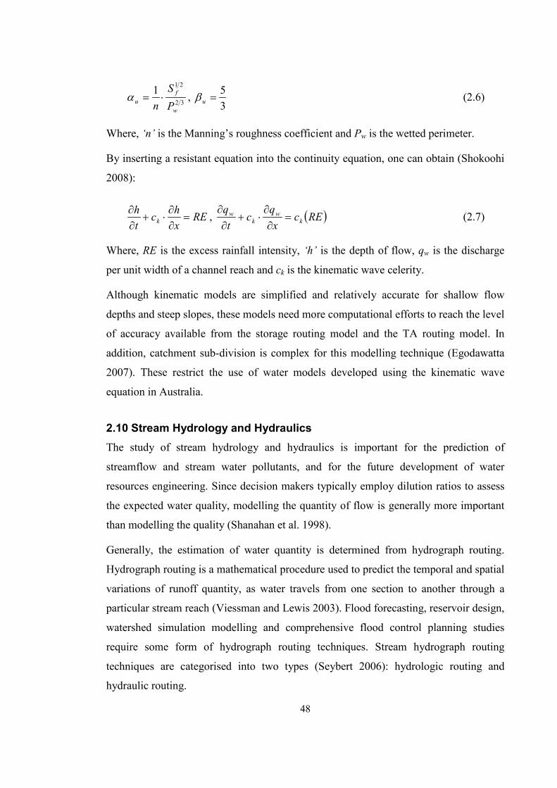
48

32

211

w

fu P

Sn⋅=α ,

35

=uβ (2.6)

Where, ‘n’ is the Manning’s roughness coefficient and Pw is the wetted perimeter.

By inserting a resistant equation into the continuity equation, one can obtain (Shokoohi

2008):

RExhc

th

k =∂∂⋅+

∂∂ , ( )REc

xq

ct

qk

wk

w =∂∂⋅+

∂∂ (2.7)

Where, RE is the excess rainfall intensity, ‘h’ is the depth of flow, qw is the discharge

per unit width of a channel reach and ck is the kinematic wave celerity.

Although kinematic models are simplified and relatively accurate for shallow flow

depths and steep slopes, these models need more computational efforts to reach the level

of accuracy available from the storage routing model and the TA routing model. In

addition, catchment sub-division is complex for this modelling technique (Egodawatta

2007). These restrict the use of water models developed using the kinematic wave

equation in Australia.

2.10 Stream Hydrology and Hydraulics The study of stream hydrology and hydraulics is important for the prediction of

streamflow and stream water pollutants, and for the future development of water

resources engineering. Since decision makers typically employ dilution ratios to assess

the expected water quality, modelling the quantity of flow is generally more important

than modelling the quality (Shanahan et al. 1998).

Generally, the estimation of water quantity is determined from hydrograph routing.

Hydrograph routing is a mathematical procedure used to predict the temporal and spatial

variations of runoff quantity, as water travels from one section to another through a

particular stream reach (Viessman and Lewis 2003). Flood forecasting, reservoir design,

watershed simulation modelling and comprehensive flood control planning studies

require some form of hydrograph routing techniques. Stream hydrograph routing

techniques are categorised into two types (Seybert 2006): hydrologic routing and

hydraulic routing.

49

2.10.1 Hydrologic Stream Routing

The first reference to routing a flood hydrograph from one stream station to another was

derived by Graeff in 1883 (Viessman and Lewis 2003). The technique was based on the

use of wave velocity and a rating curve of stage-discharge relationship. A particular

stream is modelled as a single reach or divided into several sub-reaches. When more

than one reach is used, the calculation of the furthest upstream section is done first.

Then the calculation proceeds in the downstream direction making the outflow from one

stream to the inflow for the next downstream reach.

For a particular stream reach, water entering into the reach must either exit from that

reach, or cause a change in reach storage. The simplest form of routing equation relies

on the conservation of mass and can be written as: inflow – outflow = change in storage

(Ladson 2008). Mathematical expression is:

dtdS

OI csvSS =− (2.8)

Where, Is is the inflow rate to a stream reach at the upstream section (m3/s), Os is the

outflow rate from a stream reach to the downstream section (m3/s), dScsv/dt is the rate of

change of storage volume within the stream reach at time ‘t’ and Scsv is the volume of

reach storage.

The most popular hydrologic stream routing methods are: the Muskingum method and

the Muskingum-Cunge method.

2.10.1.1 Muskingum Method

A popular hydrologic stream routing method is the Muskingum method. The method

was developed by G.T. McCarthy (1938) using studies associated with the U.S. Army

Corps of Engineers Muskingum Conservancy District Flood Control Project in Eastern

Ohio (Seybert 2006). This method is used for the calculation of an outflow hydrograph

at the downstream end of a stream reach for a given inflow hydrograph at the upstream

end. The basic assumption for the Muskingum method is that the stage-discharge

relationship is one-to-one and it is strictly applied (Cunge 1969). In addition, the cross

sectional geometry is assumed to be constant throughout a reach section.

50

The simplified storage relationship in the Muskingum method uses the geometric shapes

of a prism and wedge to represent reach storage capacity. The prism represents reach

storage volume where flow is steady, i.e. the inflow is equal to the outflow. The wedge

represents reach storage volume above the prism which is caused by a passing a flood

wave (Seybert 2006).

The Muskingum method is a finite difference solution of the storage equation. The

storage within a particular stream reach at a given time can be expressed as (Chow

1959):

( )

−+×= SD

SVSD

SVn

m

SPn

m

SPSD

SVstor OXIX

abS 1 (2.9)

Where, Sstor is the channel storage (m3), aSD and nSD are the stage-discharge

characteristics of a control section, bSV and mSV are the mirror of the stage-volume

characteristics of reach section and XP is the relative weight of the inflow and the

outflow for a particular stream reach.

The method assumes that a linear relationship exists between Sstor, IS and OS (Akan and

Houghtalen 2003). Equation 2.9 produces a linear relationship if mSV/nSD = 1. Assuming

bSV/aSD = Kstor one can get the following equation:

( )[ ]SPSPstorstor OXIXKS −+×= 1 (2.10)

Where, Kstor is the storage time constant for a particular stream reach.

Equation 2.10 states that channel storage is a function of the channel inflow and

outflow. The application of Equation 2.10 has shown that Kstor is usually reasonably

close to the wave travel time through a stream reach (Viessman and Lewis 2003). The

value of weighting factor XP varies between 0 and 0.5 with an average value of about

0.2. The behaviour of a flood wave due to the changes in the values of XP is readily

apparent as shown in Figure 2.12. The figure shows that when XP = 0.5, the result is a

perfect translation of a flood wave.

Equation 2.10 is straightforward, if the values of Kstor and XP are known. Using

subscripts 1 and 2 to denote the beginning and the end of the routing time interval ∆tR

one can obtain:

51

R

storstorSSSS

tSSOOII

∆−

=+

−+ 1,2,2121

22 (2.11)

Figure 2.12: Effect of weighting factor (Xp)

The change in reach storage during the routing interval is written from Equation 2.10:

( ) ( )( )[ ]12121,2, 1 SSPSSPstorstorstor OOXIIXKSS −−+−=− (2.12)

Substituting this into Equation 2.11 results in the Muskingum routing equation:

1211202 SMSMSMS OCICICO ++= (2.13)

in which

RPstorstor

RPstorM tXKK

tXKC∆+−

∆+−=

5.05.0

0 (2.14)

RPstorstor

RPstorM tXKK

tXKC∆+−

∆+=

5.05.0

1 (2.15)

RPstorstor

RPstorstorM tXKK

tXKKC∆+−∆−−

=5.05.0

2 (2.16)

52

It should be noted that Kstor and ∆tR must be in the same unit and CM0, CM1 and CM2 are

dimensionless Muskingum routing coefficients. The sum of the value of CM0, CM1 and

CM2 is unit:

1210 =++ MMM CCC (2.17)

Since IS1 and IS2 are known from a given inflow hydrograph and OS1 is known either

from the initial conditions or from the previous time step computations at any given

time interval, the only unknown parameter in routing Equation 2.13 is OS2.

With the predetermined values of Kstor, XP and ∆tR, routing coefficients are computed

and a general routing equation in the form of Equation 2.13 is created. The solution

begins by identifying the inflow and outflow conditions in a particular stream reach

section.

In the Muskingum method, it is assumed that water surface is a uniform unbroken

surface profile between the upstream and downstream ends of a reach section.

Moreover, the routing parameters Kstor and XP are best derived from streamflow

measurement and are not related to the channel characteristics (Akan and Houghtalen

2003; Viessman and Lewis 2003). In addition, the values of Kstor and XP are pre-

supposed to be constant throughout ranged flows. These limitations are overcome by the

Musking-Cunge method.

2.10.1.2 Muskingum-Cunge Method

The Muskingum-Cunge method is one of the attempts to overcome the limitations of the

Muskingum method. It is based on the continuity of mass equation within a channel

reach. For the general use, Cunge (1969) blended the accuracy of the diffusion wave

method for the simplicity of the Muskingum method. The input parameters, such as

length, roughness, slope and geometry allow for the computation of routing parameters

Kstor and XP for each routing interval. It is classified as a hydrologic method, yet it gives

the comparable results with hydraulic methods (Viessman and Lewis 2003). The

Muskingum-Cunge method is also a well-known method used to compute pollutographs

of stream reaches.

53

According to Cunge (1969), the finite difference form of the Muskingum equation

becomes the diffusion wave equation, if the parameters of the both methods are

appropriately related. From Equations 2.8 and 2.10, the Muskingum equation becomes:

( )[ ] SSSPSPstor OIOXIXdtdK −=−+⋅ 1 (2.18)

Substituting Qi for IS and Qi+1 for OS, and rewriting in finite difference form, we can

obtain:

( ) ( )[ ]tiP

tiP

tiP

tiP

R

stor QXQXQXQXt

K1

11

1 11 +++

+ −−×−−+∆

( )ti

ti

ti

ti QQQQ 1

11

1

21

+++

+ −+−= (2.19)

The equation to be used for routing a flood wave is obtained from Equation 2.19 by

solving for the un-known flow rate:

tiMC

tiMC

tiMC

ti QCQCQCQ 121

10

11 +

+++ ++= (2.20)

Where,

storRSR

PstorRMC Ktx

XKtC∆+−−∆

=)1(2

20 (2.21)

storRSR

PstorRMC Ktx

XKtC∆+−+∆

=)1(2

21 (2.22)

storRSR

RkSRMC Ktx

xtcxC

∆+−∆∆−−

=)1(2)1(2

2 (2.23)

Where, CMC0, CMC1 and CM2 are dimensionless Muskingum-Cunge routing coefficients.

If Kstor is assumed to be ∆xSR/ck, where ∆xSR is the length of a sub-reach then Equation

2.20 is also the finite-difference of:

0=∂∂⋅+

∂∂

SR

strk

str

xQ

ct

Q (2.24)

54

This is called a kinematic wave equation and can be derived by combining the

continuity equation and the momentum (friction) equation. The parameter ck can be

derived based on the kinematic wave theory. A discharge rating curve is necessary to

compute the value of ck and a common approach to approximate the ck is by using the

Manning’s equation (Seybert 2006). If the previous flood data are available the value of

ck can be extracted by reversing routing calculations.

The value of celerity ck can also be calculated as a function of the average flow velocity

by:

fuk uc β= (2.25)

Where uf is the average velocity (Qstr/Ax) and βu is about 5/3 for wide natural channels.

The coefficient βu comes from the uniform flow Equation 2.5. By taking the partial

derivatives Equation 2.5 produces:

fux

str

x

str uA

Qm

AQ

β=⋅=∂∂

(2.26)

Substituting these into the continuity equation:

0=∂∂

+∂∂

tA

xQ xstr (2.27)

This gives Equation 2.20; if ck = βuuf. If discharge data are available, βu can be

estimated from Equation 2.25.

The parameter XP is a dimensionless weighting factor that has a value between 0 and 0.5

and generally between 0.1 and 0.3 for natural channels (Linsley et al. 1992). When XP =

0, the volume of water in storage is purely a function of outflow alone, and XP = 0.5

indicates that the inflow and the outflow have an equal weighting in determining the

volume in storage and the routing equation produces translation without attenuation.

Cunge proposed the following equation for the determination of XP:

∆

−=SRk

P xcSqX

0

121 (2.28)

When ∆xSR = 0 (zero reach length), no translation or attenuation occurs.

55

When ∆tR < Kstor, the negative value at the outflow hydrograph can occur in the rising

limb of a hydrograph. This negative value can be avoided by choosing ∆tR, ∆xSR and

Kstor such that (∆xSRKstor)/(L∆tR) lies below the curve shown in Figure 2.13 (Cunge

1969). Model for Urban Stormwater Improvement Conceptualisation (MUSIC)

automatically sub-divides the reach length into a number of sub-sections N = ∆xSR/L,

such that (∆xSRKstor)/(L∆tR) lies below the curve shown in Figure 2.13, when the users

set the values of Kstor and XP for a stream reach. The values of Ki for all sub-reaches are

made equal such that Ki = Kstor/N, where Kstor is the value defined by the users for the

whole stream reach.

Figure 2.13: (∆xKstor)/(L∆t) vs. XP Curve

In addition, when the value of 2Ki(1-XP) for a sub-reach is less than ∆tR, the negative

value is formed in the calculation of CMC2 and ultimately in the falling limb of the

outflow hydrograph which is unrealistic. Therefore, the parameters should be selected in

such a way so that these negative values can be avoided. However, it is often difficult to

satisfy both the conditions to stop the negative values in outflow hydrographs,

especially when the value of XP is outside the range of 0.1 to 0.49 (CRC for Catchment

Hydrology 2005). To avoid this discrepancy MUSIC limits the value of XP in between

0.1 and 0.49.

56

2.10.2 Hydraulic Routing

Hydraulic routing depends on the simultaneous solution of the continuity equation and

the momentum equation for unsteady, gradually varied (non-uniform form) flow

(Seybert 2006). Differential form of the continuity (conservation of mass) equation for

the significant lateral inflow can be written as:

LTSR

TSR

fCF q

thB

xhvB

xu

A =∂∂⋅+

∂∂

⋅+∂

∂⋅ (2.29)

Where, ACF is the channel flow area, BT is the top width of a channel reach and qL is the

lateral inflow.

This equation is augmented with a conservation of momentum equation as presented by

Henderson (1966) for unsteady flow in a stream reach:

tu

gxu

gv

xhSS f

SR

f

SRf ∂

∂⋅−

∂

∂⋅−

∂∂

−=1

0 (2.30)

Where, Sf is the friction slope and ‘g’ is the acceleration due to gravity.

These are nonlinear partial differential equations that require sophisticated numerical

techniques for solution.

2.11 Water Quality Modelling Approaches An accurate estimation of water borne pollutants transferred from upstream catchments

to the downstream are crucial for the design of effective impact mitigation devices and

management strategies. If we are able to predict water quality parameters at un-sampled

locations or point with sufficient accuracy, we do not need to sample at these locations.

Therefore, mathematical approaches have become prevalent for predicting water quality

parameters of aquatic environments. The advancement of mathematical models as a tool

for the simulation of water quality followed the historical development. Computer

models are such water quality prediction tools which are widely used to simulate

different water quality parameters. Computer models of urban stormwater runoff and

pollutant loads are extremely useful in establishing whether various management

strategies to produce water quality that conforms to legislation (Zoppou 2001).

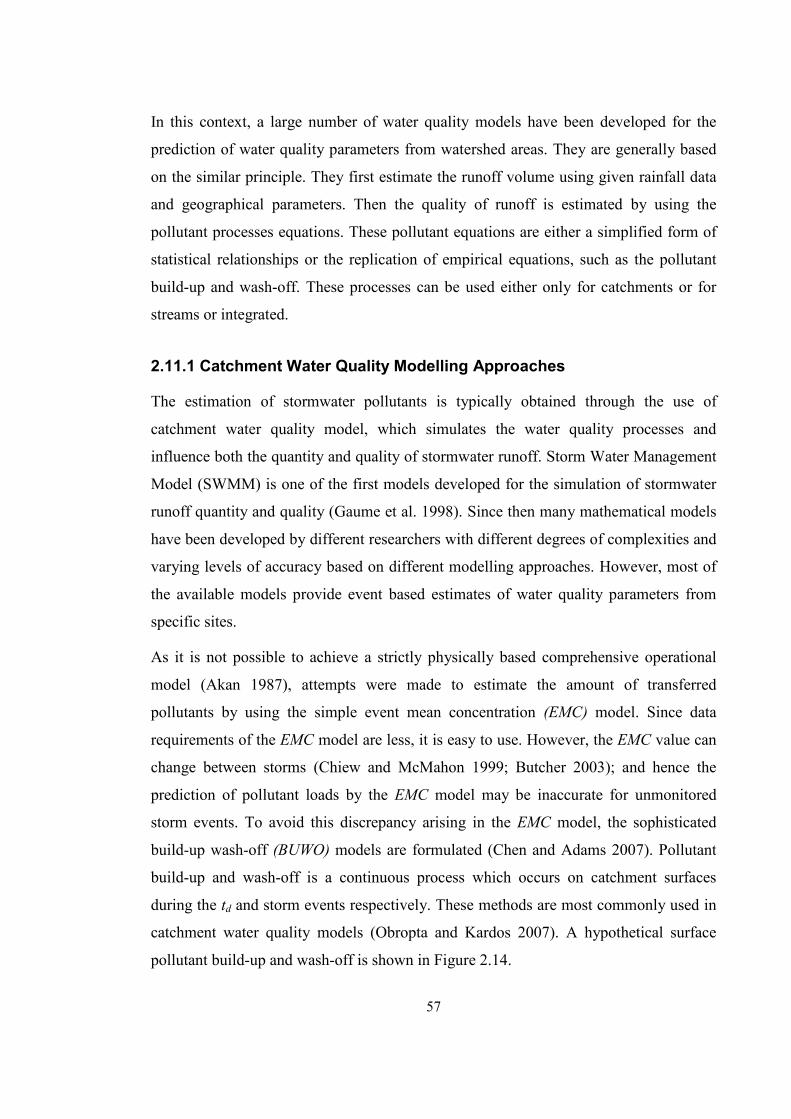
57

In this context, a large number of water quality models have been developed for the

prediction of water quality parameters from watershed areas. They are generally based

on the similar principle. They first estimate the runoff volume using given rainfall data

and geographical parameters. Then the quality of runoff is estimated by using the

pollutant processes equations. These pollutant equations are either a simplified form of

statistical relationships or the replication of empirical equations, such as the pollutant

build-up and wash-off. These processes can be used either only for catchments or for

streams or integrated.

2.11.1 Catchment Water Quality Modelling Approaches

The estimation of stormwater pollutants is typically obtained through the use of

catchment water quality model, which simulates the water quality processes and

influence both the quantity and quality of stormwater runoff. Storm Water Management

Model (SWMM) is one of the first models developed for the simulation of stormwater

runoff quantity and quality (Gaume et al. 1998). Since then many mathematical models

have been developed by different researchers with different degrees of complexities and

varying levels of accuracy based on different modelling approaches. However, most of

the available models provide event based estimates of water quality parameters from

specific sites.

As it is not possible to achieve a strictly physically based comprehensive operational

model (Akan 1987), attempts were made to estimate the amount of transferred

pollutants by using the simple event mean concentration (EMC) model. Since data

requirements of the EMC model are less, it is easy to use. However, the EMC value can

change between storms (Chiew and McMahon 1999; Butcher 2003); and hence the

prediction of pollutant loads by the EMC model may be inaccurate for unmonitored

storm events. To avoid this discrepancy arising in the EMC model, the sophisticated

build-up wash-off (BUWO) models are formulated (Chen and Adams 2007). Pollutant

build-up and wash-off is a continuous process which occurs on catchment surfaces

during the td and storm events respectively. These methods are most commonly used in

catchment water quality models (Obropta and Kardos 2007). A hypothetical surface

pollutant build-up and wash-off is shown in Figure 2.14.

58

(a) Source limiting, (b) Transport limiting

Figure 2.14: Hypothetical representations of surface pollutant load over time

(Vaze and Chiew 2002)

SWMM is one of the BUWO models, which is a widely used model to simulate

stormwater pollutants. However, the lack of data for the determination of the parameters

of BUWO models can lead to the significantly biased results in the estimation of water

borne pollutants. There is no standard form of pollutant build-up and wash-off

formulation (Shaw et al. 2010). However, there are minor variations amongst the

available formulations and their conceptual basis is the same.

The basic model for pollutant processes on a particular catchment surface can be written

as follows (Shaw et al. 2010):

BWttwt

Bttt tQPPP

kPPBW

∆

−

−+=∆+ α

max

1 (2.31)

Where, Pt is the available pollutant mass (kg) accumulated on a catchment surface at

time ‘t’, Pmax is the threshold at which additional pollutant do not accumulate on a

catchment surface (kg), kB is the pollutant build-up coefficient (kg/time), Qt is the runoff

rate (m3/time) at time ‘t’, αw is the wash-off rate constant (m-3) and ΔtBW is the time

increment for pollutant build-up or wash-off.

59

2.11.1.1 Event Mean Concentration

The event mean concentration (EMC) is a method used to characterise the concentration

of pollutants from storm water runoff into nearby waterways and receiving water

bodies. It is a statistical parameter used to present a flow weighted average

concentration of a desired water quality parameter during a single storm event

(Wanielista and Yousef 1992). An EMC model assumes a single flow weighted

concentration and can be used across an entire storm event. The EMC model is the

simplest model to calculate stormwater pollutants which is mostly useful for calculating

annual pollutant loads (Charbeneau and Barrett 1998). This is the frequently used

method to characterise stormwater loadings.

The EMC value can be determined by calculating the cumulative mass of pollutants and

dividing it by the volume of storm runoff. The classical EMC model can be

demonstrated as follows (Kim et al. 2004):

( )

( )∫

∫= T

Ts

T

c

dttV

dttPEMC

0

0 (2.32)

Where, EMC is the event mean concentration, Pc(t) is the captured pollutant loads, VTs

is the volume of runoff during the integration time interval and Ts is the duration of

storm event.

However, in most of the cases, the monitored watershed area does not represent a single

homogeneous land-use. Then the observed EMC is the runoff weighted sum of all

EMCs from the individual land-use (Butcher 2003). For these cases, the mathematical

expression of EMC can be written as follows:

( ) ( ) ( ){ }

( ) ( ){ }∑

∑

=

== n

iiciD

n

iiciDi

AR

AREMCEMC

1

1 (2.33)

Where, RD is the depth of runoff and Ac is the contributing area.

60

2.11.1.2 Pollutant Build-up

Pollutant build-up is the accumulation of contaminants on catchment surfaces prior to

rainfall events. However, during storm events, rainfall not only washes away pollutants

from catchment surfaces but also deposits its own pollutants (James and Thompson

1997). This deposition is small enough to neglect in water quality modelling.

It is widely accepted that rain washable pollutants are engendered during the td. To the

present, most of the build-up studies have been conducted by considering the td as the

most influential parameter (Egodawatta et al. 2009; Vaze and Chiew 2002; Chui 1997;

Kibler 1982; Sartor et al. 1974). For example, the first build-up assumption justified by

the work of Sartor and Boyd (1972) used the td as the most important parameter. Alley

and Smiths (1981) also developed a pollutant build-up model that included the td as an

input parameter. In addition, Soonthornnonda and Christensen (2008); Rossman (2004)

found that the accumulation pollutant loads on a catchment surface is a function of the

number of preceding dry weather days

On the other hand, some other researchers criticised this assumption. Based on the

experimental study at Belgrade in Yugoslavia and Lund in Sweden on impervious

surfaces, Deletic and Maksimovic (1998) found that the td had only a minor effect upon

the accumulation of road surface pollutants. At Aberdeen, Scotland Deletic and Orr

(2005) found that the td had a weak negative influence on the accumulation of pollutant

on catchment surfaces. Shaw et al. (2010) noted that the accumulation of pollutants on

catchment surfaces is not deterministically related to the td. These contradictory results

were due to the different geographical conditions and the time which had elapsed

between data collections.

The common variables, such as surface type, roughness, slope, land-use and weather

conditions affect the redistribution of pollutant loads; and hence the build-up rate.

Initially available pollutant is another important factor in the accumulation of water

quality pollutants which dominates the transport rate. Theoretically, it can be assumed

that pollutants on catchment surfaces accumulate uniformly. However, the rate of

pollutant build-up is significantly higher during the initial period (Ball et al. 1998;

Sartor and Boyd 1972). Then the rate decreases as the dry days increases and eventually

approaches zero due to land-use activities.

61

Egodawatta (2007) found that pollutant build-up is significantly higher during the first

two days for road surfaces and seven days for roof surfaces. Vaze and Chiew (2002)

noted that pollutant build-up on road surfaces may vary along the longitudinal direction

depending upon the presence of traffic signals and bottlenecks. In addition, the regional

and catchment management practices influence pollutant build-up and its composition

(Ball et al. 1998). Therefore, different pollutant build-up functions are used to determine

the accumulation of water quality parameters.

Usually, the accumulation of water quality parameters on a catchment surface is

presented by two main build-up functions, i.e. the linear and the non-linear. At the very

beginning, SWMM assumed that there was a linear increase of pollutants whereby a

constant amount of pollutants increased during the td (Novotny et al. 1985). The linear

pollutant build-up with the td can be written as follows:

( ) dLDt tkBd

= (2.34)

Where, ( )Dtd

B is the accumulation of pollutant on a particular catchment surface during

td, kL is the linear build-up rate constant and td is the antecedent dry time (days or hrs).

However, the linear build-up concept is not always adequate in depicting more realistic

pollutant accumulation processes on catchment surfaces (Whipple et al. 1977). Ball et

al. (1998) tested a range of models in different forms for pollutant build-up, and they

found that the power function and the hyperbolic function are the best fit pollutant

accumulation model. Therefore, Alley and Smith (1981) emphasised on the non-linear

build-up model.

The non-linear pollutant build-up process was first identified from the field data

collected by Sartor and Boyd (1972). From the non-linear build-up models, the power

function, the exponential function and the Michaelis-Menton function are the main

types found in water quality literature (Wang and Li 2009). Amongst them, the

exponential function is the most widely employed build-up model (Chen and Adams

2006). The first published pollutant accumulation model was also exponential. Most of

the available models accepted the accumulation of pollutants in the form of decreasing

rate with increasing dry days.

62

The decreasing of pollutant accumulation with increasing dry days can be expressed as

follows (Novotny et al. 1985):

d

dtwi

t BkPdt

dB−= (2.35)

Where, Pi is the sum of all the inputs and kw is the wash-off coefficient.

The above Equations 2.34 and 2.35 are based on the assumption that every storm has

the capacity to remove all the available pollutants from catchment surfaces for an

adequate duration of rainfall event. However, from the literature review, it was easily

understood that a single storm event can transport only a fraction of pollutants from a

particular catchment surface (Egodawatta et al. 2007). For example, the experimental

study by Vaze and Chiew (2002) showed that a significant rainfall event of 39.4 mm can

remove only 35% of pollutant loads. Therefore, in practice, the amount of accumulated

pollutants on catchment surfaces has two parts, i.e. pollutants build-up during the td and

residual pollutants not washed-off by the previous storm events (Chen and Adams

2007). Hence, Charbeneau and Barrett (1998) proposed the following build-up model,

which accounts for the mass not washed-off during the previous rainfall event.

( ) ( )DtRtt ddd

BBB += (2.36)

Where, ( )Rtd

B is the pollutant mass not washed off during the previous rainfall event.

2.11.1.3 Pollutant Wash-off

Pollutant wash-off is the transportation of the accumulated pollutants by surface runoff

from catchment surfaces to nearby waterways and receiving water bodies (Temprano et

al. 2006). An accurate estimation of water quality parameters entering into waterways

and receiving water bodies depends on the accurate representation of the wash-off

model (Sriananthakumar and Codner 1992). The complex process of pollutant wash-off

is determined by a number of factors. Numerous research studies were conducted in

identifying the governing variables of pollutant wash-off. However, most of the

hypotheses were based on the four influencing rainfall runoff variables, i.e. rainfall

intensity, rainfall volume, flow rate and runoff volume (Egodawatta et al. 2007).

63

According to Akan (1987), the characteristics of raindrops, overland flow and type of

pollutants affect the pollutant wash-off rate. Moreover, Bannerman et al. (1993) found

that the runoff energy has a significant influence on the pollutant wash-off process. In

addition, Chen and Adams (2007) noted that types and conditions of street surfaces, the

particle size, street cleaning and traffic density affect the pollutant wash-off rate.

Berretta et al. 2007) also noted that the dynamics of the pollutant wash-off process is

affected by hydrologic parameters, the catchment characteristics and the nature of

pollutants. Duncan (1999) and Novotny et al. (1985) noted that the amount of pollutant

washed-off from catchment surfaces is influenced by the amount of pollutant

accumulated during the td. Kibler (1982) noted that landscape modification affects the

pollutant wash-off rate.

However, it is difficult to find out the relative importance of each parameter on the

pollutant wash-off rate (Herngren et al. 2005). The interrelationships amongst different

variables show the difficulty in understanding the degree of influence of individual

variables. Therefore, different researchers proposed different pollutant wash-off models

for the estimation of pollutant loads from catchment surfaces. Most of these studies

focused on impervious surfaces, especially impervious road surfaces. There are only

few studies of pollutant wash-off rates for residential and open land areas. Even these

areas are major sources of water quality parameters in stormwater runoff

(Soonthornnonda and Christensen 2008; Bannerman et al 1993).

The wash-off formulations used in most of the existing models are very similar to

SWMM. However, these formulations are purely empirical and contain at least one

parameter which has no physical basis. SWMM’s formulations are according to the

algorithm of the first developed stormwater management model developed by Metcalf

and Eddy Inc. et al. (1971). Metcalf and Eddy Inc. et al. (1971) proposed that the rate of

pollutant wash-off from a catchment surface is proportional to the mass of pollutant

which remains on that surface.

PwBS

P WkdtdW

−= (2.37)

Where, WP is the pollutant wash-off from a catchment surface (mass) and tBS is the time

since the beginning of a storm event.

64

In urban stormwater quality modelling, Sartor et al. (1974) proposed a solution to this

exponential equation as a function of rainfall intensity and duration. Their study

concluded that the pollutant wash-off rate from an impervious surface area is

proportional to the rainfall intensity and the mass of pollutant available on a particular

catchment surface.

( ) ( )BSW

d

ItkDtP eBW −= 1 (2.38)

However, Alley (1981) modified this exponential wash-off model and showed that

pollutant wash-off is better predicted by the runoff rate instead of rainfall intensity. The

expression can be written as follows:

( ) ( )BSRW

d

tRkDtP eBW −= 1 (2.39)

Where, RR is the average runoff rate of a storm event (mm/hr) during the time step tBS.

However, many other researchers noted that pollutant wash-off can be better predicted

using the runoff volume, e.g. Deletic et al. (1997). Barbe et al. (1996) also suggested

adopting a wash-off model which is related to the runoff volume. The expression of

pollutant wash-off relationship with runoff volume can be written as:

pE

TswP VkW = (2.40)

Where, Ep is the power of wash-off parameter.

On the other hand, Akan (1987) showed that the pollutant detachment rate at any point

along a particular catchment surface is assumed to be proportional to the overland flow

bottom-shear stress and the amount of pollutant available on that surface. Assuming the

pollutant wash-off rate as proportional to the bottom-shear stress of the overland flow

and the distribution density, Akan (1987) proposed a physically-based mathematical

model. The expression can be written as follows:

AtWBS

Pd

hBSkdtdP

,0= (2.41)

Where, AtdB , is the mass of the pollutant per unit surface area.

65

However, there are many stormwater quality models which were developed based on

the assumption that the rate of pollutant wash-off is proportional to the remaining

pollutants and surface runoff (Chen and Adams 2007; Osuch-Pajdzinska and Zawilski

1998; Grottker 1987; Sartor et al. 1974).

AtwBS

P qBdtdW

dα−= (2.42)

Where, qA is the runoff rate per unit catchment area.

The primary boundary condition of these wash-off equations is the amount of pollutant

available on a catchment surface (Barbe et al. 1996) to wash-out during surface runoff

event. However, it is commonly recognised that pollutant wash-off is significantly

greater at the beginning of a storm runoff compared to the later period, after rainfall has

cleansed catchment surfaces (Novotny et al. 1985).

2.11.1.4 The First-Flush Phenomena

First-flush (FF) is a term used to refer to the higher concentration of pollutants in

stormwater runoff during the initial period of a storm event. Generally, stormwater

runoff containing a higher pollutant concentration is called FF. It is often noted that the

highest intensity of rainfall are bursts at the initial period of a rainfall event, which

could cause the higher pollutant wash-off during that period of storms and increases the

occurrence of FF.

Numerous researchers considered the FF phenomena as an important factor in

stormwater pollutant wash-off and transportation processes. They observed the highest

amount of pollutant wash-off during the initial period of a storm event. Sartor et al.

(1974) found that surface runoff from the first hour of a moderate to heavy storm would

contribute more pollutant loads than sanitary wastes of the same area during the same

time period. Egodawatta and Goonetilleke (2008) and Taebi and Droste (2004) observed

that a higher fraction of pollutant from catchment surfaces is transported during the

initial period of a storm. Therefore, Ballo et al. (2009) noted that the effects of FF are

obvious in stormwater runoff. Hence, the existence of FF should be considered in

stormwater management strategies.

66

The occurrence and the nature of FF can be influenced by a range of factors. It can vary

with the rainfall intensity, the runoff volume and the catchment characteristics.

Different hypotheses were tested to establish the relationships between FF and rainfall,

runoff, catchment area, td, and collection network characteristics. If there is a large

quantity of available pollutant then the transport rate from catchment surfaces is higher.

Therefore, FF is increased in residential areas due to stormwater runoff from roof

surfaces. Forster (1996) noted that roof surfaces produce a significant concentration of

pollutants during the initial period of surface runoff. The imperviousness of a catchment

area is also responsible for the FF phenomenon. Lee et al. (2002) observed the higher

FF occurrence for small and impervious watershed areas.

Although the occurrence of FF is commonly reported, the FF effects appear only to

limited number of pollutants and storm events (Batroney et al. 2010; Deletic and

Maksimovic 1998). Deletic (1998) observed FF during large storm events when

deposition of pollutants on catchment surface is small. In Melbourne, Australia Bach et

al. (2010) did not observe any FF for all the catchments they studied. Therefore, the

appropriateness of FF depends primarily on the nature and sources of pollution, in terms

of drainage hydrology, pollutant mobility and pollutant supply. Therefore, identification

of the existence or non-existence of the phenomenon is most critical.

FF is most important in stormwater treatment design. Pollutant collection systems

during FF are employed to capture and isolate the most polluted runoff. Stormwater

retention and detention basins are designed considering FF to treat the initial runoff

which contains a higher concentration of pollutants (Egodawatta 2007). After the time

of FF, the rest of the runoff is discharged without any treatment.

2.12 Stream Water Quality Modelling Approaches Stream water quality modelling has become an integral part of water resources planning

and water quality management options throughout the world. Stream water quality

models inquire about the description of the spatial and temporal variations of water

quality parameters. Moreover, these models are widely used to aid in water quality

surveillance and to predict water quality conditions. They are extensively used in

research as well as in the design and the assessment of water quality management

measures.

67

Due to various studies on stream water quality, there are a large number of models

available for the simulation of different water quality parameters. Since the initial study

of Streeter and Phelps (1925), models are constantly refined and updated to meet the

emerging problems of surface water pollution. Following the evolution of water quality

problems, this starting model (Streeter and Phelps model) was developed with only two

state variables. Since then more processes descriptions and variables have been

gradually incorporated into it over the past seven decades in an attempt to improve the

water quality simulation.

However, in most of the models the main processes considered are physical transport

and exchange processes (such as advection and diffusion/dispersion), physical

conversion processes, and chemical, biological and biochemical processes of water

quality parameters (Rauch et al. 1998). In most of the water quality models, these

processes are one-dimensional (1D), i.e. the changes in pollution constituents are only

taken into account along the mean stream direction and are constructed by discretisation

along stream. The dynamics of stream water quality parameters are described in the

well-known three-dimensional (3D) partial differential equation (PDE) (Cox 2003;

Chapra 1997; Thomann and Mueller 1987):

zcu

ycu

xcu

tc

zyx ∂∂⋅+

∂∂⋅+

∂∂⋅+

∂∂

),( mzyx pcfzc

zyc

yxc

x

+

∂∂⋅

∂∂

+

∂∂⋅

∂∂

+

∂∂⋅

∂∂

= εεε (2.43)

Where, c is a multi-dimensional mass concentration vector for each of the water quality

parameters, x, y, z are spatial coordinates, ux is the average longitudinal velocity

component, uy is the average transverse velocity component, uz is the average vertical

velocity component, εx is the turbulent diffusion coefficient in the longitudinal direction,

εy is the turbulent diffusion coefficient in the transverse direction, εz is the turbulent

diffusion coefficient in the vertical direction and ‘f’ is a term representing the rates of

change of state variables due to biological, chemical and other conversion processes as a

function of the concentration ‘ c ’, and the model parameters pm, which is subjected to

calibration.

68

2.12.1 Available Stream Water Quality Models

Stream water quality models are developed by a simultaneous solution of a set of

equations describing each of the pollutants involved. However, most of the equations

require the users to provide the values of the rate parameters and to calibrate these

parameters in order to achieve a fit with the observed data (Cox 2003).

Generally, there is not enough time or funding for the field investigation of water

quality parameters (Cox 2003). Therefore, stream water quality models are crucially

important for the prediction of water quality parameters within a stream reach.

Numerous examples of commercial stream water quality models (SIMCAT, TOMCAT,

QUAL2E, QUASAR, MUSIC, MIKE11 etc.) were developed for the simulation of

water quality parameters with some ranged values of the model parameters.

SIMCAT (SIMulation of CATchments) is a one-dimensional, steady state, stochastic

stream water quality model which represents the inputs from the point-source effluents.

The model can simulate pollutants either conservatively or by having the first order

decay. Although the model calculation is quick, the approach considered is over

simplistic. This model is suitable for pollutants in freshwater where sediment interaction

is negligible (Cox 2003).

TOMCAT (Temporal/Overall Model for CATchments) is essentially identical to

SIMCAT, i.e. a steady state model. However, TOMCAT allows for more complex

temporal correlations. Although the model has limited functionality in terms of

processes included, the use of seasonal statistics does allow for the potentially greater

accuracy than that could be achieved in the SIMCAT model. Nevertheless, the model is

limited by over simplistic ascriptions of flow and water quality processes even with the

excellent data. In addition, due to the inclusion of some seasonality, it is not a dynamic

model and cannot examine short term variability, such as the diurnal effects.

The stream water quality model QUAL2E was developed and released by the United

States Environmental Protection Agency (US EPA) in 1985. The QUAL2E is a steady

state model for the conventional water quality parameters in 1D stream and well-mixed

ecosystems. The model is similar to SIMCAT and TOMCAT models. However, the

conceptualisation of QUAL2E is rather more advanced than these two models (Cox

2003).

69

The basic theory of QUAL2E is based on the assumption that major transport

mechanisms, advection and dispersion are significant only along the main direction of

flow. QUAL2E is considered as one of the most widely used stream water quality

simulation models throughout the world (Brown and Barnwell 1987). Although the

model is widely used, it did not get great exposure in the UK because it is a steady state

model and there is no stochastic component. Moreover, the model is much complex and

requires extensive data. Like any other water quality model, QUAL2E needs to be

correctly calibrated and verified for a particular stream for the reliable prediction of

water quality parameters. In addition, QUAL2E and other similar models do not address

a number of practical problems, such as stormwater flow events (Shanahan et al. 1998).

MIKE 11 is a 1D (cross-sectionally averaged) dynamic stream water quality model

which was developed by the Danish Hydraulic Institute (DHI). MIKE 11 is a widely

used hydraulic as well as water quality model used to assess the impact of pollutant

discharges into streams and estuaries. The model consists of a set of flow and water

quality modules. The model is used for the simulation of water quantity and quality,

such as sediment transport in estuaries, streams, irrigation channels and other water

bodies. In addition, the model accounts for photosynthetic production, respiration,

atmospheric re-aeration, BOD decay and nitrification. The number of water quality

parameters included depends on the level of model being run. Although MIKE 11 is an

advanced water quantity and quality model, a common problem for this complex model

is the requirements for large amounts of data which may not always be available.

QUASAR (QUAlity Simulation Along River Systems) is a dynamic stream water

quality model which describes the time varying (i.e. dynamic) transport and

transformation of solutes in branched river systems using 1D, ordinary and lumped

parameters for a differential equation of the conservation of mass (Cox 2003).

MUSIC (Model for Urban Stormwater Improvement Conceptualisation) was developed

by the CRC for Catchment Hydrology, Australia. Although it is a catchment water

quality model, the Muskingum-Cunge theory was used for routing streamflow and water

quality parameters. The model is stochastic and can simulate water quality parameters

with some treatment options. However, the model does not consider internal

conversions of the reactive pollutants within stream reach.

70

All of the developed models contain similar assumptions and limitations that need to be

understood for a meaningful interpretation of the model simulation (Cox 2003).

However, it is difficult to identify a single model that is good enough to simulate all of

the pollutant processes. Some of them were developed for specific sites and are not

useful for other areas. For example, due to the stochastic components and the lack of

commercial exposure, SIMCAT and TOMCAT are not generally used outside the UK

(Cox 2003). QUAL2E incorporated degradation of organic materials, growth and

respiration of algae, nitrification (considering nitrite as an intermediate product),

hydrolysis of organic nitrogen and phosphorus, reaeration, sedimentation of algae,

organic phosphorus and organic nitrogen, sediment uptake of oxygen and sediment

nutrients release. MIKE 11 was developed on the basis of modules, e.g. rainfall-runoff

component, a hydrodynamic module, a water quality module and a sediment transport

module which are mixed of the conceptual and physics based models (Merritt et al.

2003). The modules can be combined and simulate advection-dispersion, water quality,

sediment transport, eutrophication and rainfall-runoff.

Although the processes formulation of MIKE 11 is similar to QUAL2E, there are some

remarkable differences. The most important difference is the division of organic matter

into dissolved and suspended fractions in MIKE 11. The description of phosphorus

cannot be compared because in MIKE 11, phosphorus is estimated in another module.

Neither MIKE 11 nor QUAL2E makes an attempt to describe populations of bacteria.

MUSIC considers water quantity as well as pollutant loads (SS, TN, TP and gross

pollutants) as conservative substances which are unusual to other models. However,

MUSIC is widely used in Australia for predicting stormwater quality pollutants. There

are variations amongst the available stream water quality models in terms of their

complexity, number of parameters, computation time and processes involved.

2.12.2 Sedimentation Processes

Water quality of seas, lakes and streams depends on the concentration of fine sediments

(especially clay and silt particles) brought from upstream catchments with surface

runoff (Rimkus et al. 2007). During the period of intense rainfall events, the sediment

particles are transferred to nearby waterways and settled on the stream bed and on

floodplains especially during the low flow conditions.

71

From the primary view point of erosion, deposition, navigation and flood defence, the

mechanism of sedimentation has become considerable interest to hydraulic engineers,

coastal engineers, geologists, hydrologists and geographers (Yang 2005). The

sedimentation phenomena further play an important role in the evaluation of earth

surfaces topology especially in river beds, reservoirs, estuarine and coastal regions

(Zhou et al. 2003).

The transported sediment affects not only the cross sectional geometry of waterways,

but also the hydrodynamic conditions of fluid in motion. The suspended load changes

the fluid density, which is generally taken as constant in the hydrodynamic modelling. If

SS transport and deposition is not taken care properly, further remedy is needed. Lin and

Namin (2005) noted that long-term morphological processes are involved with the

transport of heavy metals and toxic wastes via the adsorption on sediment particles.

Therefore, sufficient understanding of sedimentation processes is essential for integrated

river management and river engineering. Depending on the size and density of bed

materials and flow conditions, sediment particles are divided into two main categories,

i.e. bed load and suspended load. However, the scope of this thesis is limited to

suspended load.

Over recent years, a number of SS models ranging from 1D to 3D equations were

developed. This is because of the sedimentation rate depends on a large number of

factors which form the flow structure. The volume and distribution of the deposited

sediment depends on the distribution and the duration of flow, vegetation on stream

banks, the concentration of incoming sedimentation, the hydrological and other

conditions (Vaikasas and Rimkus 2003).

The process of sediment can be illustrated from the well-known advection-diffusion

Equation 2.43. For the purpose of water quality modelling, some simplifications of the

equation can be made by reducing the number of spatial dimensions. This is reasonable

because for relatively shallow streams, the mixing depth is short and thus a depth

integrated (i.e. 2D) form can be applied (Cox 2003).

Dy

ch

yhxc

hxhy

cu

xc

ut

c ssy

ssx

ssy

ssx

ss −

∂∂⋅

∂∂

⋅+

∂∂⋅

∂∂

⋅=∂∂⋅+

∂∂⋅+

∂∂

εε 11 (2.44)

72

Where, ssc is the depth average SS concentration vector and ‘D’ is a term representing

the rate of SS deposition or erosion (kg/m3/s).

In the calculation of SS deposition, the term ‘D’ is of great importance which is

introduced through the bed boundary conditions. For steady flow problems, the

dispersion is often negligible and can be omitted for the simplification. Then it produces

an ordinary differential equation (ODE) which is easy to solve and analyse (Cox 2003;

Rauch et al. 1998).

Vaikasas and Rimkus (2003) determined the SS deposition rate (Dss = Dsed.h) of sand

particles by the concept of suspension transport capacity of a particular stream:

sw

trssinssss w

qqq

D ⋅−

= ,, (2.45)

Where, Dsed is the decrease in sediment flow rate due to sedimentation (kg/m3/s), Dss is

the deposition of SS per unit area of stream bottom (kg/m2/s), qss,in is the SS flow rate per

unit width (kg/m/s), qss,tr is the transport of SS per unit width (kg/m/s), qw is the

streamflow rate per unit width of reach (m2/s) and ws is the settling velocity or fall

velocity of particles (m/s).

When applying this Equation 2.45, one must know the effective transport capacity

(qss,tr) of that flow. However, SS transport is a complex phenomenon with the sediment

undergoing a series of processes such as erosion, deposition, and advective and

diffusive transportation. Numerous formulas were proposed for the calculation of qss,tr.

In most of the cases, the model for the estimation of SS transportation were developed

by applying the most common methods proposed by van Rijn (1984a, 1993) and

Bagnold (1966).

When the bed-shear velocity exceeds the particle fall velocity, upward turbulent forces

may be higher than the submerged weight of the particles and as a result suspension of

particles occurs (van Rijn 1993). However, the concentration of SS is higher close to the

bottom and gradually decreases with the distance up from the bed. The depth integrated

SS transportation proposed by van Rijn (1984a, 1993) can be expressed as follows:

δhcuFq DStrss =, (2.46)

73

Where, cδ is the reference level concentration of SS at height ‘δ’ above bed level, u is

the depth average flow velocity (m/s) and FDS is the dimensionless shape factor, which

is expressed as follows (van Rijn 1984a, 1993):

( )∫ ⋅⋅=h

a

fDS hzd

cc

uu

Fδ

(2.47)

Bagnold (1966) also proposed a SS transport model based on the energy balance

concept relating to the power of a particular stream. The equation can be expressed as

follows:

( )bs

ssstrtrss e

wue

pq −⋅⋅= 1, (2.48)

Where, pstr is the available stream power per unit bed area, es is the suspension

efficiency factor (suspension work rate per unit stream power), eb is the bed-load

transport efficiency factor (bed-load work rate per unit stream power) and us is the

transport velocity of SS (m/s).

There are also other models available for the estimation of SS transportation rate.

However, all of the models proposed by different authors are based on experiments

performed in different flow conditions; therefore they produce different results. In

addition, there are only a few numbers of models available for the generic application of

the SS simulation. The lack of accepted fundamental principles and the demand for the

practical application stimulated the engineers and scientists to improve existing

sediment transport equations.

2.12.3 Reactive Pollutants Processes

The solute transport equations described in the previous section 2.12.2 are sufficient for

simulating substances which do not undergo any transformation or reaction within a

stream reach. However, for certain pollutants (e.g. nutrients, BOD, DO), these equations

need modification, because they are affected by a number of factors. Without advection,

dispersion and external inputs, internal transformations of these pollutants occur within

stream.

74

Similar to the SS processes, equations for the reactive pollutants can be derived from the

advective-diffusive Equation 2.43. For 1D flow after neglecting the diffusion term, the

advective-diffusive equation becomes a simple ordinary differential equation (Marsili-

Libelli and Giusti 2008).

( )RRR CfK

dtdC

−= (2.49)

Where, CR is the concentration of reactive pollutant (mg/L), KR is coefficient for the

reaction parameter or rate coefficient and f(CR) is the general reactive term for the

pollutant concentration CR.

This is the simplest form of the commonly used equation in water quality models for the

reactive pollutants (Cox 2003). For the prediction of reactive pollutants, this f(CR) is

highly significant because it represents the pollutant processes.

For modelling the nitrogen processes, Equation 2.49 can be used as a first order decay

function. However, most of the widely used models (e.g. QUAL2E, MIKE 11) present

more detailed processes of nitrogen. The nitrogen processes can be presented by organic

nitrogen, ammonium (NH4), ammonia (NH3), nitrite (NO2) and nitrate (NO3).

Nevertheless, in general, the last one (i.e. NO3) is present in the highest quantity. In the

nitrogen cycle, organic nitrogen is produced by algae, and removed by hydrolysis into

ammonium and by the settling process. Ammonium is reduced from the water column

by the nitrification process. Ammonium is also released by algal respiration and reduced

during photosynthesis. Again the denitrification process generates ammonium and

releases it to water. On the other hand, the nitrate concentration is affected by

nitrification and denitrification. Nitrite is produced from ammonium in the first stage of

denitrification and removed by oxidation of nitrite to nitrate. Finally, nitrate in the water

column is consumed by algae. Since the action of micro-organisms and chemical

reactions convert these forms sequentially, it is convenient to consider TN in modelling

(Boorman 2003).

Similar to the nitrogen processes, the phosphorus processes can be described from

Equation 2.49. Phosphorus can exist as either organic or dissolved fractions. Organic

phosphorus is produced by algae and removed by the normal decay and settling.

75

However, the dissolved phosphorus is produced due to the decay of organic phosphorus

and its release from sediment, and removed by algal photosynthesis. Since these

processes are very complex and difficult to include in modelling due to the lack of

rigorous data, it is convenient to consider TP in water quality modelling instead of

fragmental components.

Other than SS and nutrients, BOD and DO are the most important water quality

parameters for the degradation of stream water quality. The process of BOD can be

derived by the oxidation procedure and by the settling procedure. In stream water, BOD

processes are simulated as being removed by biological oxidation and sedimentation;

and accumulated due to algal death. However, some models (e.g. MIKE 11) include the

contribution of BOD from re-suspension. The total process of DO can be derived by the

reaeration, algal photosynthesis and respiration, sediment oxygen demand, nitrification

and use of oxygen to satisfy BOD within the water column.

However, most of the rate parameters of reactive pollutants are temperature dependent

which itself is modelled as a conservative variable. The function to represent the

temperature effect on rate coefficients is:

20−= TerefrefTe kk θ (2.50)

Where, kTe is the process rate at (Te) ºC (1/day), kref is the process rate at a reference

temperature, always 20 ºC and θref is the temperature correction factor of the reactive

pollutants at reference temperature.

2.13 Integrated Models From the evolution of environmental pollution, many processes of the environment

were developed and modelled. The detailed models were developed to describe

individual needs and objectives of environmental problems. However, currently adopted

stormwater quality models are unable to reproduce the historical pollutographs

accurately and reliably (Cheah and Ball 2007). Therefore, decision makers at all levels

are feeling dissatisfied with the outcomes resulting from ‘narrowly-focused incremental

and disjointed’ environmental management (Margerum and Born 1995).

76

Many of the present researchers are arguing that earlier approaches failed to deal with

many interconnections. Therefore, Parker et al. (2002) noted that environmental

problems of the 21st century cannot be considered in isolation. The integration is

essential to address the current and future environmental problems.

The integrated modelling approach will set priorities and implement natural resource

management options in a better way. According to Jakeman and Letcher (2003), the

integrated approach will allow us to develop a better understanding of the

interdependencies of the processes involved and may lead to the identification of the

outcomes which are considered better tradeoffs than pre-specified optima. Furthermore,

Rotmans and Asselt 1996) stated that integrated models are useful: (i) to analyse the

dynamic behaviour of complex systems, (ii) to show interrelations and feedback

amongst the various issues, (iii) to make uncertainties explicit and analyse the

accumulation of uncertainties and (iv) to develop end-to-end strategies. In addition, the

integrated approach will allow us to represent complexities and interactions within and

between different environmental systems effectively. Hence, the integrated modelling

approach will become an objective of government policy internationally.

Although the integrated modelling approach is known, there is no generally agreed upon

the definition of what constitutes integration. Different disciplines focus on different

scales for the integration of modules from different sources (Parker et al. 2002).

Different researchers described various forms of integration. For example, linking

models with GIS (Geographic Information System), integrating with software,

integration of more than one model, or even stakeholder participation are different

forms of integration.

Rotmans and Asselt (1996) provided a definition of integrated assessment: “Integrated

Assessment is an interdisciplinary and participatory process of combining, interpreting

and communicating knowledge from diverse scientific disciplines to allow a better

understanding of complex phenomena”. Risbey et al. (1996) stated that models that

attempt to integrate information by linking mathematical representations of different

components of natural and social systems is one way of creating an integrated model. In

addition, the integration of different disciplines is required to gain insights into complex

processes.

77

In the case of water quality, the integrated modelling approach can be defined as

modelling of interactions between two or more physical systems (Rauch et al. 2002),

e.g. catchment hydrology and water quality, stream hydrology, hydraulics and water

quality. An integrated water quality model is the combination of more than one model

to observe the changes in water quality parameters passing through nearby waterways

into receiving water bodies, such as the integrated catchment-stream water quality

model.

The process of integrated modelling approach should be considered as an important

product for any particular project. According to Parker et al. (2002), by recognising the

approach of integrated model, earlier forms of system models can be replaced with

integrated models which will incorporate different dimensions of the environment and

facilitate scenario generation and decision support functions. However, the development

of an integrated model is a challenging task (Rauch et al. 2002). The main constraint is

the complexity of systems that prevents existing simple deterministic models.

Furthermore, data availability is a severe constraint for obtaining more informed and

confident decision support through an integrated model.

2.14 Conclusions This chapter reviewed the current state of knowledge with respect to water quality

parameters, their sources, hydrology, current water quality modelling approaches and

the related issues. A list of considerations which are appropriate for model selection was

also presented in this chapter. Finally, the chapter reviewed the issues related to the

integrated modelling approach. From the discussion of the literature review, important

conclusions relating to hydrologic, hydraulic and water quality regime can be

summarised.

The primary water borne pollutants identified in the literature include litter, SS,

nutrients, hydrocarbons, heavy metals and organic carbon. Among them SS and

nutrients are mainly responsible for the degradation of the quality of waterways and

receiving water bodies. Most of the other pollutants are chemically adsorbed to the

particulate pollutants.

78

Although human existence is impossible without water, excesses in human activities are

responsible for the degradation of water quality and water environments. Due to the

various anthropogenic activities, road surfaces are recognised as the largest contributor

of water quality parameters, which are mainly generated from vehicles. All other

impervious and pervious surfaces are the dominant sources of pollutants under certain

conditions. The extent of pollutant contribution varies depending on the characteristics

of catchment surfaces. Types of land-use also play an important role in the

accumulation of water quality parameters.

Pollutant loads from different sources are transported into waterways and receiving

water bodies and deteriorate the quality of aquatic ecosystems. To address water quality

concerns adequately, it is important to measure the amount of pollutants present on

catchment surfaces and their transportation during storm events. Proper estimation of

pollutant loads helps to control their transportation by guiding watershed management

authorities for the implementation of appropriate management options. However,

management strategy based on the test results are costly, time consuming and

sometimes impossible. The use of mathematical models has become a common practice

of analysis, aimed at understanding of the cause-effect relationships between emissions

and water body quality, assessing the impact of the changes and to design as well as to

assess the effectiveness of mitigation measures.

The modelling technique plays an important role for the development of appropriate

watershed management strategies and to support decision making processes. The

models are used for the analysis of various scenarios and for the evaluation of

alternative management operations to achieve desired objectives. The goal of a model is

to reduce the complexity and effort spent on hand computation and analysis.

At present, numerous excellent and elegant water quality models are available and new

models are appearing regularly to provide tools for water quality managers and

regulators for the protection and improvement of aquatic environments from the impact

of pollution and for the adoption of appropriate management options. However, there

are no adequate guidelines available to select appropriate modelling options which can

be used to simulate various processes. The lack of user friendliness and proper selection

of the model parameters further hinder the application of water quality models.

79

Different algorithms are employed in different models to estimate water quality

parameters. These differences among sub-models are due to the different levels of

complexity of systems modelled and are likely to be due to the uncertainty of differently

measured data. Few models exist which are appropriate for providing the accurate

pollutant loads prediction and identification of the critical pollutant sources. A range of

problems including over parameterisation, data requirements, inappropriate structure

and unsuitability of model assumptions often constrains the use of a complex model.

Therefore, more complex models are often no more successful.

There are two major components of water quality models, i.e. the quantity and quality

components. The estimation of the quantity characteristics is a well-developed field.

There are various tools and established methods for the estimation of water quantity.

However, the estimation process of quality has only been developed recently. The lack

of understanding of the pollutant processes and underlying variables, the use of a quality

model can often leads to gross errors. An extensive amount of data is needed to calibrate

the water quality component of a model.

This literature review showed that no one’s model could provide all of the functionality,

which is essential in the prediction of water quality parameters. The models were

developed based on the experimental study and for a particular situation. Therefore, the

generic application of a particular water quality model is often difficult. In addition,

detailed models of catchments and stream water describe the performance according to

the individual needs and objectives. Since most of the models were developed for a

particular purpose, it is unfair to set one model against another in terms of broad

applicability. Due to the large variability of errors, it is difficult to draw specific

conclusions on superiority of one model over another.

The literature review also identified that no water quality models were developed to

simulate catchment and stream water quality parameters integratively. However, the

growing demand for the integrated water quality model originates from current surface

quality policy programs. The earlier approaches to environmental management usually

failed to deal with interconnections, complexities, multiple perspectives, multiple uses

and resulting cross-cutting externalities. Today’s challenge is to move from such

individual considerations of system performances to an integrated approach.

80

Environmental problems of the 21st Century are public and non-exclusive. To achieve

an integrated and sustainable future, instead of a fragmented disciplinary future, there is

a call for the integrated modelling approach. For any particular project, the process of

integrated assessment and modelling is important. Therefore, the literature review

highlighted the necessity for guidelines or improved methods and also the need for the

further development of integrated models for the prediction of water quantity and

quality. There is no doubt that in-depth knowledge of the integrated modelling approach

is crucially important to implement BMPs and to safeguard water quality, such as the

design of pollutant control structures.

81

Chapter 3 Model Development

3.1 Introduction Chapter 2 illustrates the stipulations for the development of an integrated water quality

model. This chapter demonstrates the development of an integrated catchment-stream

water quality model which continuously simulates different water quality parameters.

The integrated model is comprised of two individual models, i.e. the catchment water

quality model and the stream water quality model. These models can be used separately

or in combination to predict water quality parameters. The output from the catchment

water quality model can be used as the input for the stream water quality model.

Each of the models was developed with two basic components, i.e. the water quantity

component and the water quality component. The quantity model estimates hydrographs

generation at the point of interest; while the quality model estimates the amount of

transported pollutants into waterways and receiving water bodies. The quantity model

was incorporated with the quality model to be able to continuously simulate different

water quality parameters. The main aim was to determine the quantity and quality of

surface runoff discharged from catchment surfaces into waterways and receiving water

bodies during rainfall events by using an integrated modelling approach.

The three basic water quality parameters were included for the development of the

integrated model, i.e. SS, TN and TP. However, for the stream water quality model, the

BOD process was also included. The specific rational for the selection of these

pollutants is not available, however they can be summarised. Water is the most

important vector for transporting pollutants from upstream catchments into waterways

and receiving water bodies, and therefore its inclusion is essential. SS is an important

agent for the transportation of adsorbed pollutants, such as heavy metals, pesticides and

other pollutants. They also play a significant role in evolving the shape of estuaries and

coastlines (Boorman 2003). Moreover, the growth rate of photosynthetic organisms is

reduced by the high concentration of SS (Akan and Houghtalen 2003).

82

Nitrogen has many sources within catchments including the deposition, fertilizer

application, discharge from sewage treatment plants etc. In the form of ammonia,

nitrogen is highly toxic to fish and aquatic organisms (Bowie et al. 1985). In addition,

nitrogen is generally a limiting nutrient to algal growth. Like nitrogen, too much

phosphorus also leads to the excessive plant growth. Both of these nutrients (nitrogen

and phosphorus) are the critical components of eutrophication. BOD is considered to be

one of the most important water pollutants for the degradation of stream water quality.

These pollutants are often used as the indicators of the quality of water as well as their

impact on receiving water. On the other hand, the estimation of TN and TP from the

direct proportioning to the SS loadings increases errors due to the uncertainty in the

prediction of SS loads (Butcher 2003). In addition, for water quality management

strategies, Russel et al. (1998) noted that the consideration of only the dissolved portion

of pollutants will underestimate the total nutrients flux. Therefore, TN and TP were

considered in developing a meaningful model and a water quality prediction tool.

Overall based on data availability and other important factors in water quality

modelling, these water quality parameters were selected for the development of the

integrated model. However, other pollutants can be incorporated with the model.

This chapter starts with the construction of a catchment water model, including

catchment hydrology and pollutant processes. After that, the chapter focuses on the

development of a stream water quality model, including the quantity and quality of

stream water and their progressions. Finally, the chapter discusses the integration of the

catchment water quality model with the stream water quality model.

3.2 Catchment Water Quality Model General strategies and programs for watershed management always depend on the

catchment water quality modelling results which involve both the runoff and the

pollutants processes (Chang et al. 2007). Therefore, over the years, various catchment

water quality models have been developed for the estimation of surface runoff and

pollutant loads. A comprehensive catchment water quality model facilitates the

simulation of both surface runoff and pollutant loads simultaneously (Chiew and

McMahon 1997). Hence, Amoudry (2008) noted that modelling the quality of water

required describing both pollutant and ambient water motions and their interaction.

83

The catchment water quality model was developed for the continuous simulation of

stormwater quantity and quality during the period for which rainfall data are given to

the model. The model is comprised of two sub-models, i.e. the runoff model and the

pollutant model. The runoff model also known as the hydrologic model enables the

simulation of catchment hydrological processes via a range of commonly applied

rainfall loss and routing methods. The pollutant model estimates the amount of pollutant

accumulated during the td and the amount washed-off during surface runoff event. The

model also recognises the influence of effective impervious area of catchment surfaces.

The basic functions of the model are similar to the comprehensive hydrological and

water quality simulation model, SWMM. However, SWMM does not consider the

rainfall kinetic energy which is considered as an important factor for the pollutant wash-

off as found in recent studies, such as Shaw et al. (2010); Egodawatta et al. (2007). The

model has the option to consider the rainfall intensity from which the kinetic energy can

be calculated directly. The final output of the model is the quantity and quality of

stormwater runoff at a catchment outlet.

The major advantage of the model is that it can be used for either the continuous or the

event based simulation of hydrology and water quality parameters associated with

surface runoff during rainfall events. In addition, the model is capable of considering

both the pollutant loads and concentration of catchment surfaces. The model thus

improves the estimation of pollutant loads entering into waterways and receiving water

bodies.

3.2.1 Runoff Model

It is well recognised that stormwater pollutants cannot be predicted accurately without

proper estimation of the runoff quantity. Usually, the runoff quantity from a storm event

is measured by the traditional rainfall-runoff models (Kokken et al. 1999). However, the

output of such models is used to investigate wider environmental problems, such as the

water quality issues (Christophersen and Wright 1981). Therefore, rainfall-runoff

transformation is considered to be the key component of any stormwater quality model

because it characterises the runoff generation mechanism and determines the degree of

model complexity (Chen and Adams 2007).

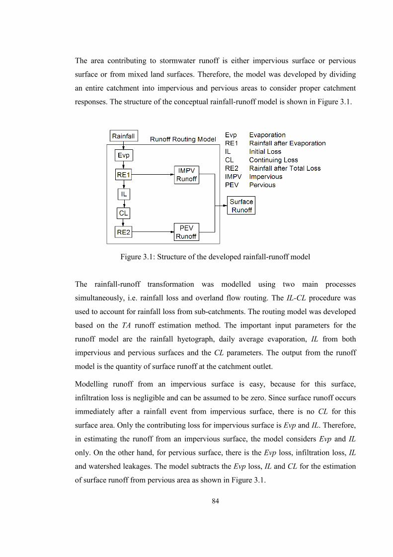
84

The area contributing to stormwater runoff is either impervious surface or pervious

surface or from mixed land surfaces. Therefore, the model was developed by dividing

an entire catchment into impervious and pervious areas to consider proper catchment

responses. The structure of the conceptual rainfall-runoff model is shown in Figure 3.1.

Figure 3.1: Structure of the developed rainfall-runoff model

The rainfall-runoff transformation was modelled using two main processes

simultaneously, i.e. rainfall loss and overland flow routing. The IL-CL procedure was

used to account for rainfall loss from sub-catchments. The routing model was developed

based on the TA runoff estimation method. The important input parameters for the

runoff model are the rainfall hyetograph, daily average evaporation, IL from both

impervious and pervious surfaces and the CL parameters. The output from the runoff

model is the quantity of surface runoff at the catchment outlet.

Modelling runoff from an impervious surface is easy, because for this surface,

infiltration loss is negligible and can be assumed to be zero. Since surface runoff occurs

immediately after a rainfall event from impervious surface, there is no CL for this

surface area. Only the contributing loss for impervious surface is Evp and IL. Therefore,

in estimating the runoff from an impervious surface, the model considers Evp and IL

only. On the other hand, for pervious surface, there is the Evp loss, infiltration loss, IL

and watershed leakages. The model subtracts the Evp loss, IL and CL for the estimation

of surface runoff from pervious area as shown in Figure 3.1.

85

The runoff model can predict surface runoff based on different hydrologic

considerations. The runoff calculation can be done from impervious and pervious

surfaces separately for any given duration of rainfall. The total runoff at the catchment

outlet is assumed to be the combination of area-weighted runoff from impervious and

pervious surfaces of a particular catchment. General equation of the surface runoff

calculation can be written as follows:

( )[ ]( )[ ]

−−−

−=

pevimpvpevaT

impvaTS

LLIMPVLRALRIMPVAQ

0

peva

pevaimpv

impva

LRLRL

LR

>

≤<

≤

(3.1)

Where, QS is the surface runoff, IMPV is the percent imperviousness of a particular

catchment, Ra is the rainfall, Limpv is the rainfall loss from impervious surface area and

Lpev is the rainfall loss from pervious surface area.

3.2.1.1 Rainfall Loss Model

The governing rainfall abstraction/losses estimation is difficult over an entire

catchment. To overcome difficulties in the spatial variability of rainfall, the topography,

and the characteristics of catchments (such as vegetation and soils), simplified lumped

conceptual models are used. In this thesis, rainfall loss is divided and modelled into the

three categories, i.e. the Evp loss, IL and CL. Since the IL-CL method is a widely used

model in Australia, the current model was developed based on Evp and the IL-CL

model. The users have the option to provide the average value of the Evp loss.

The part of rainfall loss which occurs at the early part of a storm event is called IL.

After the initial time period, this loss disappears. The value of IL can vary depending

upon the characteristics of a particular catchment and weather conditions. Tularam and

Ilahee (2007) noted that the rainfall duration is also an important factor in the

calculation of IL. However, this loss is considered as fixed and most of the time, the

value of IL is derived from literature. Therefore, in the developed model, the users have

an option to provide the value of IL as a constant input value. It was mentioned earlier

that the model estimates impervious surface runoff and pervious surface runoff

separately. Hence, there are two different options to provide the value of IL for

impervious surface and for pervious surface.

86

Besides IL, all other rainfall losses that could occur through the remaining storm period

are usually categorised as CL. The values of CL depend on the type of surface areas of a

particular catchment. The usual practice of CL consideration is constant (Rahman et al.

2002a). However, Ilahee and Imteaz (2009) presented a detailed study using the IL-CL

model for many eastern Australian catchments. Their study concluded that the values of

CL are higher at the beginning of a rainfall event and gradually decreases with the time

as rainfall continues.

To calculate the values of CL, the developed model allows the users in using any of the

available three different methods, i.e. constant, exponentially decreasing or linearly

decreasing. By allowing the different options for CL estimation, the model becomes

flexible and is improved. Equations 3.2 to 3.4 represent CL models for constant,

exponential decreasing and logarithmic decreasing respectively. The choice and validity

of a model depends on the availability of data and the runoff calculation processes.

CLCL δ= (3.2)

BStCLCL eBACL −−= (3.3)

)( BSCL tLogCCL −= (3.4)

Where, CL is the continuing loss (mm/hr), ACL is the parameter for exponential

decreasing CL, BCL is the coefficient for exponential decreasing CL, CCL is the

parameter for logarithmic CL, tBS is the time since commencement of a rainfall event

(mins) and δCL is the constant value of CL.

3.2.1.2 Routing Model

While watershed runoff models can be formulated with various degrees of complexity

based on different methodological considerations, the catchment hydrologic model for

this research study was developed using the TA method to represent the partial area

runoff contribution of a particular catchment. It was recognised that a fundamental part

of a runoff hydrograph development is the use of the TA method. Since the TA method

is one of the most widely used and suitable model for watershed routing, it was used in

the generation of catchment runoff.

87

Over intervening years to present, ILSAX, DRAINS are widely used models in

Australia. They also utilises the basic TA method to estimate both impervious surface

and pervious surface runoff. In addition, Kull and Feldman (1998) found that 40% of

the US Corps of Engineers projects use the TA technique in the rainfall-runoff model.

The general equation of the TA method which gives a net hydrograph due to rainfall

excess can be written as follows:

( ) ( ) ( ) 11

+−=∑= kjsub

j

kkjS AREQ (3.5)

Where, ‘j’ is the time step and Asub is the area between two consecutive isochrones.

Using Equation 3.5, the developed model generates separate hydrographs for

impervious and pervious surfaces. These hydrographs are combined to calculate the

total runoff hydrograph. According to Equation 3.5, the watershed area should first be

divided into sub-areas before applying the TA method.

3.2.1.3 Catchment Sub-division

Since the entire catchment area does not contribute to surface runoff at the same time

during a rainfall event, the area is divided into a suitable number of sub-areas to

describe the proper watershed responses. Various sub-catchment flows are combined

and routed through the system to a catchment outlet. However, it is unfeasible to sub-

divide a catchment into an infinitive number of sub-catchments. In this study, the

fundamentals of catchment sub-area division were based on the tc because it is assumed

that after the tc the entire area of a catchment contributes to surface runoff. The model

was developed by dividing a catchment into sub-catchments along watershed lines

(isochrones lines). The developed model has the two different options for the division of

a particular catchment area into sub-areas:

Sub-area division by the user

Sub-area division by the model

The users have the choice to select any of these two procedures based on available data.

When isochrones data are available for a particular catchment, the users can divide the

entire catchment area into sub-areas from these isochrones data. The developed model

has an option to account sub-areas and corresponding imperviousness.

88

However, where isochrones data are not available, several empirical methods were

developed for the delineation of isochrones. For this thesis, the empirical technique

from the HEC-1 was used for the automatic sub-division of a particular catchment by

the model. Since this technique gives the better results for watershed area sub-divisions

(Shokoohi 2008), it was adopted in the hydrological model development. In the HEC-1

user manual, it was noted that this empirical technique is useful for watershed areas,

where physiographic data are not available. For this technique, the watershed area is

assumed to be a parabola. Where sub-catchment areas are not available, the program

utilises a dimensionless TA curve as follows:

5.1414.1 DCD tA = ( )5.00 <≤ DCt (3.6)

( ) 5.11414.11 DCD tA −−= ( )0.15.0 <≤ DCt (3.7)

Where, AD is the dimensionless catchment area, which is the proportion of the

considered area to the total area, and tDC is the dimensionless time meaning the

proportion of the considered area cumulative time to the tc. The whole procedure can be

described as follows. From Equation 3.6

5.1414.1 DCD tA =

5.11 414.1 DCT

tAAA

==⇒

TDC AtA *414.1 5.11 =⇒

Tc

At

tA *414.15.1

1

∆=⇒

Tc

At

tA **1414.15.1

1

∆=⇒

Tc

At

tA **2414.15.1

2

∆=⇒

89

Tc

At

tA **3414.15.1

3

∆=⇒

........................................................

........................................................

Tc

i At

tiA **414.15.1

∆=⇒

From Equation 3.7

( ) 5.11414.11 DCD tA −−=

( ) 5.11 1414.11 DCDT

tAAA

−−==⇒

( ){ } TDC AtA *1414.11 5.11 −−=⇒

Tc

At

tA *1414.115.1

1

∆−−=⇒

Tc

At

tA **11414.115.1

1

∆−−=⇒

Tc

At

tA **21414.115.1

2

∆−−=⇒

Tc

At

tA **31414.115.1

3

∆−−=⇒

........................................................

........................................................

90

Tc

i At

tiA **1414.115.1

∆−−=⇒

Where,

∑=i

iT AA1

(3.8)

Δt Travel time of water parcel between two isochrones

3.2.1.4 Time of Concentration

Recognising the importance of the tc in the hydrologic design and calculation, the

hydrologists have developed numerous methods to calculate the tc for a particular point

(generally the furthest) within a particular watershed area to the outlet (Fang et al.

2007). However, these methods are not based on the theory of fluid mechanics. They

were developed based on the analysis of one or more data sets and called empirical

methods. Although these developed equations are empirical, many of them generally

require the use of lumped basin parameters, such as basin area, flow path length,

average slope, Manning’s ‘n’, channel factors, runoff coefficient, rainfall intensity,

hydraulic radius. Some of the tc computation methods are single, lumped parameter

empirical equations and others divide the flow path into different hydraulic flow

conditions and then sum the travel time from separate segments of flow. The developed

model allows the users to select any of the three established methods for the calculation

of the tc for a particular catchment. These methods are widely used in Australia and can

be discussed as follows.

Where a complete procedure based on the observed data is not available, the Bransby

Williams formula was adopted as an arbitrary but reasonable approach. The method is

described as follows:

5.01.058

eTc SA

Lt = (3.9)

Where, tc is the time of concentration (minutes), ‘L’ is the length of the main channel

(km), AT is the area of the watershed in km2 and Se is the equal area slope of the main

stream projected to the catchment outlet (m/km).

91

The Pilgrim and McDonald formula developed in 1982 is based on the typical

conditions in eastern New South Wales, Australia. This method is also used in Victoria

for the estimation of the peak discharge of a rainfall event. The formula was developed

for the estimation of critical rainfall duration as the tc. Pilgrim and McDonald (1982)

recommended using this formula for a catchment area of up to 250 km2. The formula is

expressed as:

38.06.45 Tc At = (3.10)

In the south-western part of Western Australia, the Flavelt (1983) formula is

recommended. This area includes jarrah forest with lateritic and loamy soils, low jarrah

forest with sandy soils and karri forest with loamy soils. The expression for the Flavelt

formula is:

54.06.138 Tc At = (3.11)

3.2.2 Pollutant Model

Over recent years, water resources management authorities emphasised the need for the

development of strategies for water quantity and water quality together (Fulazzaky et al.

2010). In this study, the pollutant component of the catchment water quality model was

developed and integrated with the developed hydrologic model to present a meaningful

catchment water quality response. The pollutant model consists of two main functional

sub-components, i.e. the pollutant build-up and the pollutant wash-off. The build-up

model estimates the accumulation of water quality parameters within a catchment

surface during the td. The wash-off model estimates the amount of transferred pollutants

into nearby waterways and receiving water bodies with surface runoff.

According to the research literature, there are various techniques available for the

estimation of pollutant build-up and wash-off from a particular catchment surface. Ball

et al. (1998) suggested that instead of using one model, alternative models with different

degrees of complexity and computation effort should be employed for the prediction of

water quality parameters. The best selected model depends on the information needed

which differs for each water ecosystem, individual management alternatives, and

different institutional objectives and constraints (Laenen and Dunnette 1997).

92

Most of the currently available stormwater quality models were developed for

impervious surface only. Stormwater quality models for pervious area are very limited.

However, water quality parameters from pervious area also play an important role in

polluting aquatic environments (Deletic and Maksimovic 1998; Grottker 1987).

Therefore, water quality parameters from pervious surface area should be considered in

any water quality study. In this study, the catchment water quality model was developed

by considering the three different types of surface areas: (i) impervious surface, (ii)

pervious surface and (iii) mixed surfaces (partly impervious and partly pervious).

The model allows the users to use different build-up and wash-off coefficients for

impervious and pervious surface of a particular catchment area. These coefficients for

build-up and wash-off models are determined by the land-use of those areas from

observed or experimental water quality data. Finally, based on the calculated

coefficients, the model estimates pollutant loads or concentrations at the catchment

outlet.

For the practical application of the model, the minimum allowable value of the td was

assumed to one day (24 hrs). This means that if the td was less than 24 hrs, pollutant

build-up on catchment surface was negligible and assumed to be zero. Keeping in mind

our objectives, it seemed logical to take the model similar to the widely used model

SWMM as the basis for the catchment water quality model. The concept of SWMM was

considered because adoption of a widely used equation gives confidence to the practical

application of any water quality model (Boorman 2003). The main mathematical

processes adopted in developing both pollutant build-up and wash-off models is

described as follows.

3.2.2.1 Pollutant Build-up Model

The td is expected to have a significant influence on the accumulation of water quality

parameters on catchment surfaces. However, pollutant build-up on catchment surfaces

continues during rainfall events (Bouteligier et al. 2002). The effect of build-up at this

time period is negligible; and hence can be discarded for the simplicity. Therefore, Chui

(1997) noted that the most important parameter for modelling pollutants build-up in a

particular catchment surface is the td.

93

In this research project, the explicit relationship between the pollutant accumulation and

the td was used for the development of the build-up model. The build-up model was

developed based on the assumption that on a clean surface, water quality parameters

accumulate until a maximum value is attained. Considering the td as the key variable

including other hypothesises, the developed catchment water quality model described

pollutant build-up by the three separate functions for impervious and pervious surfaces

of a particular catchment:

Power function

Exponential function

Saturation function

With the nature of the pollutant accumulation, an efficient, reliable and convenient

model can be selected from the above mentioned functions.

3.2.2.1.1 Power Function Build-up Model

The power function pollutant build-up equation is the best generic form for the

accumulation of water quality parameters on catchment surfaces (Owusu-Asante and

Stephenson 2006; Ball et al. 1998). The power function build-up model considers that

the pollutant build-up on a catchment surface increase with the increasing number of

dry days until a maximum limit is reached (Egodawatta 2007; Rossman 2004; Ball et al.

1998). The power function pollutant build-up model is described according to the

following Equation 3.12:

( )( ) ( ) ( ){ }( ) ( ) ( ) ( ) ( ) ( ){ }

+×××

××=

spBtspCsFsA

spCsFsAMinspB

DtspC

dimpc

impc

t

d

d ,,

,,, ,

2

1

3 (3.12)

Where, ( )spBdt

, is the accumulation of the pollutant ‘p’ (kg) on the land surface ‘s’

during the td, Ac(s) is the contributing area of the catchment (km2), Fimp(s) is the

impervious or pervious fraction of the land surface ‘s’, C1(p,s) is the maximum amount

of pollutant that can be accumulated on the land surface ‘s’ (kg/km2), C2(p,s) is the

coefficient for the pollutant build-up parameter ( )3.2 Cdaykmkg − , C3(p,s) is the

exponent for the pollutant build-up parameter and td is the number of antecedent dry

days.

94

3.2.2.1.2 Exponential Function Build-up

The exponential pollutant build-up model assumes that the accumulation of pollutants

on a catchment surface occurs as an exponential function with an upper limit

asymptotically (Rossman 2004). Many catchment water quality models employ the

exponential build-up representation because it is simple and can be derived as a first

order process (Kim et al. 2006). In this thesis, the exponential build-up model was

developed as a function of build-up rate coefficient and the td as follows:

( )( ) ( ) ( ){ }( ) ( ) ( ) ( ) ( ) ( ){ }

+−×××

××= − spBespCsFsA

spCsFsAMinspB

Dttk

impc

impc

t

d

dpd ,1,

,,,

1

1 (3.13)

Where, kp is the pollutant accumulation rate coefficient (1/day).

3.2.2.1.3 Saturation Function Build-up

The saturation build-up function assumes that the accumulation of pollutants on a

particular catchment surface occurs as a linear rate and continuously declines until the

saturation value is reached (Rossman 2004). The saturation build-up function is

presented as follows:

( )( ) ( ) ( ){ }( ) ( ) ( )

( ) ( ) ( )

++

×××

××

=spB

tspttspCsFsA

spCsFsA

MinspBDt

dp

dimpc

impc

t

d

d ,,

,

,,

, 1

1

(3.14)

Where, tp(p,s) is the half saturation constant (the days to reach half of the maximum

build-up) for the pollutant ‘p’ to the land surface ‘s’.

3.2.2.2 Pollutant Wash-off Model

The pollutant wash-off model simulates the removal of the accumulated pollutants from

a particular catchment surface into nearby waterways and receiving water bodies during

rainfall events. However, in the areas with larger rainfall events, the accumulated

pollutants can be washed-off completely by more frequent storms. As a result, the

succeeding storm may produce the same or even more runoff as the preceding storm but

may produce considerably smaller storm pollutant loads (Barbe et al. 1996).

95

From the literature review of the thesis, it was understood that the amount of pollutant

wash-off is significantly influenced by the available pollutants on a particular catchment

surface. Therefore, the pollutant wash-off model of this research project was developed

by the integration of the rainfall-runoff transformation and pollutant build-up model.

The wash-off process follows a suitable depletion law and thus influences the actual

pollutant concentration that is transported through a catchment outlet into nearby

waterways and receiving water bodies. The pollutant wash-off approaches used in this

study are based on the model developed by Rossman (2004). Similar to the pollutant

build-up model, the wash-off model was presented by three different functions as

follows:

Power function wash-off

Rating curve wash-off

Exponential function wash-off

These three wash-off functions represent the pollutant transport capacity of surface

runoff from a particular catchment area (Barbe et al. 1996). These functions were

developed to consider the wash-off from impervious and pervious surfaces separately.

These functions consider the three influential variables, i.e. the rainfall intensity, the

rainfall duration and the runoff volume. Due to their highly correlation with each other,

the individual influence cannot be clearly discerned (Chiew and McMahon 1999; Chui

1997).

3.2.2.2.1 Power Function Wash-off

The power function wash-off model assumes that the amount of pollutants removed by

stormwater runoff from a particular catchment surface is proportional to the product of

the runoff rate per unit area raised to some power and the available pollutants on that

catchment surface.

In this study, the power function pollutant wash-off model was developed by assuming

that the removal of stormwater pollutant as proportional to the amount available at a

catchment surface and directly related to surface runoff discharged from that catchment.

According to this assumption, mathematical expression of the power function wash-up

model is expressed as follows:

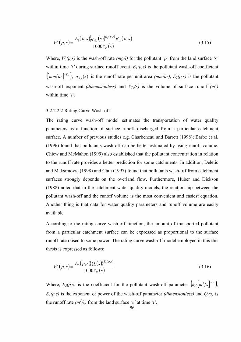
96

( ) ( ) ( ){ } ( ) ( )( )sV

spBsqspEspW

Ts

tspE

tAt

d

1000,,

,,

,12

= (3.15)

Where, Wt(p,s) is the wash-off rate (mg/l) for the pollutant ‘p’ from the land surface ‘s’

within time ‘t’ during surface runoff event, E1(p,s) is the pollutant wash-off coefficient

[ ]( )2Ehrmm − , )(, sq tA is the runoff rate per unit area (mm/hr), E2(p,s) is the pollutant

wash-off exponent (dimensionless) and VTs(s) is the volume of surface runoff (m3)

within time ‘t’.

3.2.2.2.2 Rating Curve Wash-off

The rating curve wash-off model estimates the transportation of water quality

parameters as a function of surface runoff discharged from a particular catchment

surface. A number of previous studies e.g. Charbeneau and Barrett (1998); Barbe et al.

(1996) found that pollutants wash-off can be better estimated by using runoff volume.

Chiew and McMahon (1999) also established that the pollutant concentration in relation

to the runoff rate provides a better prediction for some catchments. In addition, Deletic

and Maksimovic (1998) and Chui (1997) found that pollutants wash-off from catchment

surfaces strongly depends on the overland flow. Furthermore, Huber and Dickson

(1988) noted that in the catchment water quality models, the relationship between the

pollutant wash-off and the runoff volume is the most convenient and easiest equation.

Another thing is that data for water quality parameters and runoff volume are easily

available.

According to the rating curve wash-off function, the amount of transported pollutant

from a particular catchment surface can be expressed as proportional to the surface

runoff rate raised to some power. The rating curve wash-off model employed in this this

thesis is expressed as follows:

( ) ( ) ( ){ } ( )

( )sVsQspE

spWTs

spEt

t 1000,

,,

34

= (3.16)

Where, E3(p,s) is the coefficient for the pollutant wash-off parameter [ ]( )43. Esmkg − ,

E4(p,s) is the exponent or power of the wash-off parameter (dimensionless) and Qt(s) is

the runoff rate (m3/s) from the land surface ‘s’ at time ‘t’.

97

3.2.2.2.3 Exponential Wash-off

The exponential wash-off model estimates the decreasing pollutant concentration of a

given accumulated pollutant with increasing time since the start of a rainfall event.

Different derivations of this equation are used in the various stormwater quality models.

The most common form of the exponential function assumes that the rate of pollutant

wash-off from a particular catchment surface is proportional to the product of available

pollutant which remains on that surface and the rainfall intensity. The expression can be

written as follows.

Wdt

dWwα−= (3.17)

Where, ‘W’ is the pollutant wash-off and αw is the wash-off rate constant.

Assuming αw varies with the direct proportion to the rainfall intensity, I(s) i.e. αw =

E5(p,s)I(s), Equation 3.17 becomes:

( ) ( )WdtsIspEdW ,5−=

Integrating the equation with respect to ‘t’:

( ) ( )∫∫ −= WdtsIspEdW ,5

( ) ( )∫ ∫−=

⇒ dtsIspE

WdW ,5

( ) ( ) constCtsIspEW +−=⇒ ,ln 5 (3.18)

When the time, t = 0, then dt

BW = and the value of the constant become:

( )dtconst BC ln=

Substituting the value of the constant in Equation 3.18 one can obtain:

( ) ( ) ( ) ( )dt

BtsIspEW ln,ln 5 +−=

( ) ( ) ( ) ( )tsIspEBWdt

,lnln 5−=−⇒

98

( ) ( )tsIspEBW

dt

,ln 5−=

⇒

( ) ( )[ ]tsIspEBW

dt

,exp 5−=⇒

( ) ( )[ ]dt

BtsIspEW ,exp 5−=⇒

Therefore, the amount of pollutants removed from a particular catchment surface at any

time ‘t’:

WBWdtt −=

( ) ( )[ ]{ }dd ttt BtsIspEBW ,exp 5−−=⇒

( ) ( ){ }[ ]tsIspEBWdtt ,exp1 5−−=⇒

More specifically the equation can be written as follows:

( ) ( ){ }[ ]conv

tt

tsIspEBW d

δ,exp1 5−−

=⇒

Where, Wt is the pollutant wash-off within time ‘t’ and δconv is the conversion factor.

=11000 Ts

conv

Vδ

WhenWhen

t

t

WW

isis

inin

loads

ionconcentrat

In this research study, the exponential wash-off model is expressed as follows:

( )( ) ( )( ) ( )

( )sVspBe

spWTs

ttsIspE

td

1000,1

,,5 ××−−

= (3.19)

Where, E5(p,s) is the wash-off exponent (1/mm) for the pollutant ‘p’ from the land

surface ‘s’ and I(s) is the rainfall intensity (mm/hr) on the land surface ‘s’.

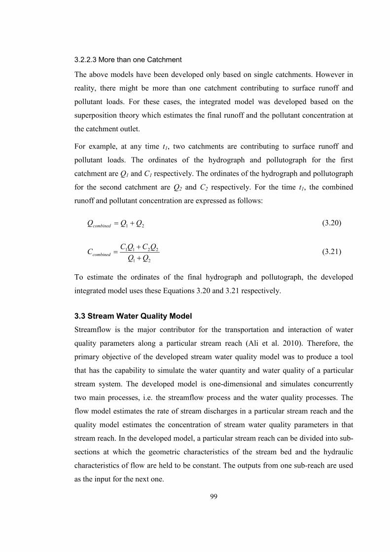
99

3.2.2.3 More than one Catchment

The above models have been developed only based on single catchments. However in

reality, there might be more than one catchment contributing to surface runoff and

pollutant loads. For these cases, the integrated model was developed based on the

superposition theory which estimates the final runoff and the pollutant concentration at

the catchment outlet.

For example, at any time t1, two catchments are contributing to surface runoff and

pollutant loads. The ordinates of the hydrograph and pollutograph for the first

catchment are Q1 and C1 respectively. The ordinates of the hydrograph and pollutograph

for the second catchment are Q2 and C2 respectively. For the time t1, the combined

runoff and pollutant concentration are expressed as follows:

21 QQQcombined += (3.20)

21

2211

QQQCQCCcombined +

+= (3.21)

To estimate the ordinates of the final hydrograph and pollutograph, the developed

integrated model uses these Equations 3.20 and 3.21 respectively.

3.3 Stream Water Quality Model Streamflow is the major contributor for the transportation and interaction of water

quality parameters along a particular stream reach (Ali et al. 2010). Therefore, the

primary objective of the developed stream water quality model was to produce a tool

that has the capability to simulate the water quantity and water quality of a particular

stream system. The developed model is one-dimensional and simulates concurrently

two main processes, i.e. the streamflow process and the water quality processes. The

flow model estimates the rate of stream discharges in a particular stream reach and the

quality model estimates the concentration of stream water quality parameters in that

stream reach. In the developed model, a particular stream reach can be divided into sub-

sections at which the geometric characteristics of the stream bed and the hydraulic

characteristics of flow are held to be constant. The outputs from one sub-reach are used

as the input for the next one.

100

The stream water quality model was developed with the same water quality parameters

(i.e. SS, TN and TP) of the catchment water quality model. However, for the survival of

fish species, and other aquatic plants and organisms, DO is significantly important

parameter for all waters. In addition, within streams biochemical oxygen demand

(BOD) is another important parameter for the simulation of accurate DO in stream water

(Boorman 2003). Therefore, these two parameters (i.e. DO and BOD) were incorporated

in the development of the stream water quality model with the catchment water quality

model’s pollutants.

A conflicting issue in the current water quantity and quality modelling techniques is that

the hydraulic radius is assumed to be equal to the flow depth. This assumption is valid

for the wide streams. For the streams with small width, this assumption leads to the

formation of gross error. To avoid discrepancy in this study, the hydraulic radius of a

particular stream reach is determined from the depth of flow by introducing a

compensation factor.

3.3.1 Streamflow Model

The streamflow model was developed by considering the well-known Muskingum-

Cunge method of stream routing. The major advantage of the Muskingum-Cunge

method is that it allows better definition of the physical characteristics of a particular

stream reach (Seybert 2006). Since the method is simple, efficient and relatively

accurate, it has been widely accepted and used in practice (Ponce et al. 1996; Barry and

Bajracharya 1995). The method was theoretically derived by Cunge (1969) by assuming

and strictly applying one-to-one stage-discharge relationship. A brief description of the

Muskingum-Cunge method is described as follows.

The equation of continuity (or storage equation) for unsteady flow through a stream

reach can be presented as:

dtdS

QQ csvoutin =− (3.22)

Where, Qin is the inflow rate into a stream reach at the upstream section (m3/s) and Qout

is the outflow rate from that reach to the downstream section (m3/s).

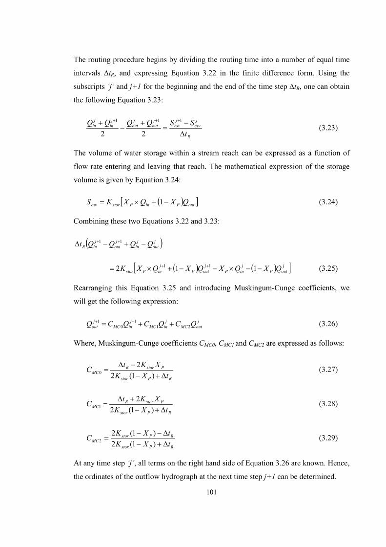
101

The routing procedure begins by dividing the routing time into a number of equal time

intervals ∆tR, and expressing Equation 3.22 in the finite difference form. Using the

subscripts ‘j’ and j+1 for the beginning and the end of the time step ∆tR, one can obtain

the following Equation 3.23:

R

jcsv

jcsv

jout

jout

jin

jin

tSSQQQQ

∆−

=+

−+ +++ 111

22 (3.23)

The volume of water storage within a stream reach can be expressed as a function of

flow rate entering and leaving that reach. The mathematical expression of the storage

volume is given by Equation 3.24:

( )[ ]outPinPstorcsv QXQXKS −+×= 1 (3.24)

Combining these two Equations 3.22 and 3.23:

( )jout

jin

jout

jinR QQQQt −+−∆ ++ 11

( ) ( )[ ]joutP

jinP

joutP

jinPstor QXQXQXQXK −−×−−+×= ++ 112 11 (3.25)

Rearranging this Equation 3.25 and introducing Muskingum-Cunge coefficients, we

will get the following expression:

joutMC

jinMC

jinMC

jout QCQCQCQ 21

10

1 ++= ++ (3.26)

Where, Muskingum-Cunge coefficients CMC0, CMC1 and CMC2 are expressed as follows:

RPstor

PstorRMC tXK

XKtC∆+−

−∆=

)1(22

0 (3.27)

RPstor

PstorRMC tXK

XKtC∆+−

+∆=

)1(22

1 (3.28)

RPstor

RPstorMC tXK

tXKC∆+−∆−−

=)1(2)1(2

2 (3.29)

At any time step ‘j’, all terms on the right hand side of Equation 3.26 are known. Hence,

the ordinates of the outflow hydrograph at the next time step j+1 can be determined.

102

In some cases, the continuously varying storage delay time with discharge is awkward.

However, this difficulty is overcome if the delay time is thought of as reach length

divided by the wave celerity which varies continuously with the discharge. This concept

is useful in understanding the non-linear routing processes. For the estimation of the

variable Kstor, the developed model adopted the following equation:

ghx

cxK SR

k

SRstor

∆=∆≈ (3.30)

3.3.2 Stream Pollutant Model

The quality component of the stream water quality model was developed to describe

and predict the observed effect of the change in water quality parameters within a

stream system. The model was developed by considering the physical, chemical and

biological changes of stream water quality parameters. The idea was to help in

developing an effective stream water quality management tool for the protection and

improvement of aquatic ecosystems of stream environments from the impact of water

pollution.

The construction of the stream pollutant model started with the development of the SS

processes modelling. The main processes involved in the SS simulation are the

deposition and transportation. Since other pollutants are related to SS, the model for SS

was developed first. After the development of the SS model, the BOD, TN and TP

models were developed for the continuous simulation of these water quality parameters.

There are two different options for the input parameters of the model. In the first option,

the input pollutant loads are coming from the developed catchment water quality model;

while in the second option, the input pollutants data are given by the users for an

upstream section of a particular stream reach. Moreover, the temperature effect of the

rate parameters was also considered in the development of the stream water quality

model because the temperature has a moderating effect on many stream water quality

parameters. The model was developed for the prediction of the mentioned water quality

parameters to guide management authorities for the implementation of appropriate

management options.

103

3.3.2.1 Suspended Sediment Model

It is widely recognised that the water quality parameter, suspended sediment (SS) is

considered to be one of the major water pollutants of streams. Therefore, measurement

of SS is important for the management of stream environments. However, the spatial

patterns of the hydraulic variables (e.g. flow depth and velocity) and the

sedimentological variables (SS concentration and deposition) are extremely complex to

an accurate estimation of SS (Nicholas and Walling 1998). Now, there are only

empirical models available and their solutions are performed based on the certain

assumptions. Therefore, further research on the SS processes is still necessary to better

understand these processes.

In this study, the SS model was developed based on the concept of streamflow, the

bottom boundary condition, the near-bed reference concentration, the transportable

sediment concentration, the critical bed-shear stress for deposition, and critical flow

velocity. The model is one-dimensional and simulates concurrently two main processes,

i.e. the sediment transport and the particle deposition. For the development of the SS

model, widely used equations were modified and used for the simulation of SS

transportation and deposition. The transport model estimates the transportation rate of

SS for a particular stream reach under the given characteristics of that reach. The

transport model proposed by van Rijn (1984a, 1993) was modified and used in this

study. The deposition model calculates the deposition of SS based on the characteristics

of sediment particles.

The model was developed based on the following assumptions: (1) width of the stream

is not too large compared to the depth of flow (i.e. it is not wide channel), (2) the inflow

sediment is coming only after rainfall events and (3) there is no re-suspension of

particles already deposited onto the stream bed. The first assumption was realistic to the

Australian conditions; because most of the creeks/streams in Australia have a relatively

small width. The second assumption was again based on the Australian conditions.

Most of the streams in Australia have no base flow and there is flow only during a

rainfall event. Hence, no sediment is transported during the dry periods, i.e. days

without rain. The third assumption was made to make the model structure simple and

user friendly.

104

The advantage of the model is that it can be applied to all streams for the prediction of

non-cohesive SS transportation and deposition along a particular stream reach. The

model was developed as a tool for the routine morphological computations in daily

water resources engineering practices. Practical problems such as sedimentation in

dredged channels, trenches, reservoirs and basins can be benefited through the use of

such a model. For a known particle size of the inflow sediment, the developed model is

capable of predicting the transportation and deposition rate of SS to a particular stream

reach.

3.3.2.1.1 Deposition of SS

The main factors determining the deposition of SS are low flow velocity and the amount

transported from upstream catchments (Rimkus et al. 2007). There is high concentration

of SS close to the bottom of stream and the thickness of this layer increases when the

sediment concentration of the entire flow increases. The saturation degree of the

sediment at the bottom layer regulates the deposition rate. However, high flow velocity

and turbulence hinder the sediment particles from settling onto the stream bottom. The

deposition begins when the concentration of sediment in the bottom layer becomes high

enough to dampen the turbulence to a necessary degree. Decrease in the turbulence at

the bottom layer allows sediment particles to fall to the bed of stream. Therefore, the

critical velocity and the transportable sediment concentration are used for the

calculation of the SS deposition (Rimkus and Vaikasas 1999).

The deposition of SS in a stream bed can be derived from the concept of the

transportable sediment concentration, the critical bed-shear stress, or critical flow

velocity (Vaikasas and Rimkus 2003). The mathematical expression of SS deposition

can be written as follows:

( )( ) ( )

( ) stw

ttrsstinsstD w

qqq

SS ⋅−

= ,, (3.31)

Where, (SSD)t is the deposition rate of SS per unit of bottom area (kg/m2/s) at time ‘t’,

(qss,in)t is the inflow rate of SS (kg/m/s) per unit width at time ‘t’, (qss,tr)t is the SS

transport rate per unit width (kg/m/s) at time ‘t’ and (qw)t is the water flow discharge per

unit width (m2/s) at time ‘t’.

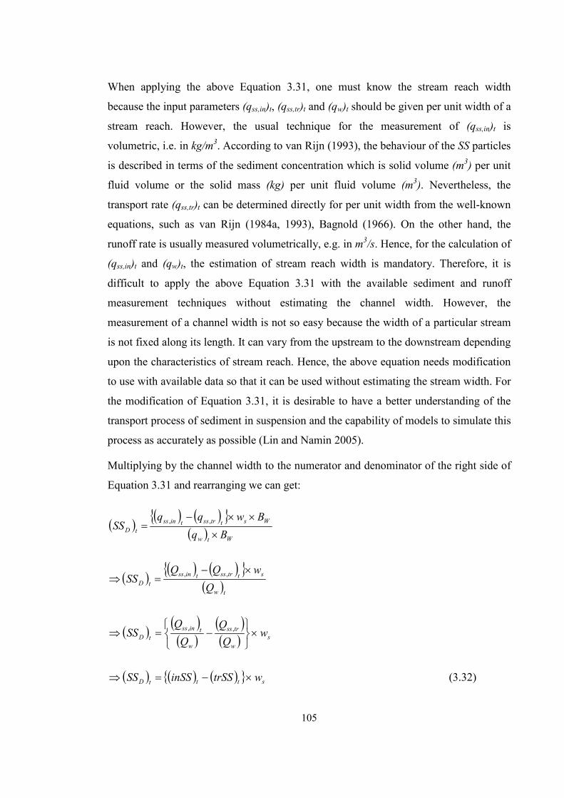
105

When applying the above Equation 3.31, one must know the stream reach width

because the input parameters (qss,in)t, (qss,tr)t and (qw)t should be given per unit width of a

stream reach. However, the usual technique for the measurement of (qss,in)t is

volumetric, i.e. in kg/m3. According to van Rijn (1993), the behaviour of the SS particles

is described in terms of the sediment concentration which is solid volume (m3) per unit

fluid volume or the solid mass (kg) per unit fluid volume (m3). Nevertheless, the

transport rate (qss,tr)t can be determined directly for per unit width from the well-known

equations, such as van Rijn (1984a, 1993), Bagnold (1966). On the other hand, the

runoff rate is usually measured volumetrically, e.g. in m3/s. Hence, for the calculation of

(qss,in)t and (qw)t, the estimation of stream reach width is mandatory. Therefore, it is

difficult to apply the above Equation 3.31 with the available sediment and runoff

measurement techniques without estimating the channel width. However, the

measurement of a channel width is not so easy because the width of a particular stream

is not fixed along its length. It can vary from the upstream to the downstream depending

upon the characteristics of stream reach. Hence, the above equation needs modification

to use with available data so that it can be used without estimating the stream width. For

the modification of Equation 3.31, it is desirable to have a better understanding of the

transport process of sediment in suspension and the capability of models to simulate this

process as accurately as possible (Lin and Namin 2005).

Multiplying by the channel width to the numerator and denominator of the right side of

Equation 3.31 and rearranging we can get:

( ) ( ) ( ){ }( ) Wtw

WsttrsstinsstD Bq

BwqqSS

×

××−= ,,

( ) ( ) ( ){ }( )tw

sttrsstinsstD Q

wQQSS

×−=⇒ ,,

( ) ( )( )

( )( ) s

w

trss

w

tinsstD w

QQ

QQ

SS ×

−=⇒ ,,

( ) ( ) ( ){ } stttD wtrSSinSSSS ×−=⇒ (3.32)

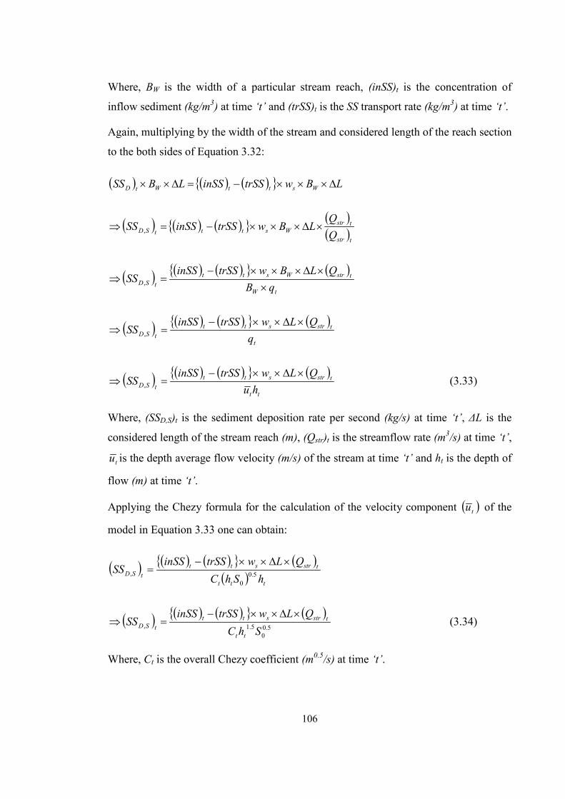
106

Where, BW is the width of a particular stream reach, (inSS)t is the concentration of

inflow sediment (kg/m3) at time ‘t’ and (trSS)t is the SS transport rate (kg/m3) at time ‘t’.

Again, multiplying by the width of the stream and considered length of the reach section

to the both sides of Equation 3.32:

( ) ( ) ( ){ } LBwtrSSinSSLBSS WsttWtD ∆×××−=∆××

( ) ( ) ( ){ } ( )( )tstr

tstrWstttSD Q

QLBwtrSSinSSSS ×∆×××−=⇒ ,

( ) ( ) ( ){ } ( )tW

tstrWstttSD qB

QLBwtrSSinSSSS

××∆×××−

=⇒ ,

( ) ( ) ( ){ } ( )t

tstrstttSD q

QLwtrSSinSSSS

×∆××−=⇒ ,

( ) ( ) ( ){ } ( )tt

tstrstttSD hu

QLwtrSSinSSSS

×∆××−=⇒ , (3.33)

Where, (SSD,S)t is the sediment deposition rate per second (kg/s) at time ‘t’, ΔL is the

considered length of the stream reach (m), (Qstr)t is the streamflow rate (m3/s) at time ‘t’,

tu is the depth average flow velocity (m/s) of the stream at time ‘t’ and ht is the depth of

flow (m) at time ‘t’.

Applying the Chezy formula for the calculation of the velocity component ( )tu of the

model in Equation 3.33 one can obtain:

( ) ( ) ( ){ } ( )( ) ttt

tstrstttSD hShC

QLwtrSSinSSSS 5.0

0,

×∆××−=

( ) ( ) ( ){ } ( )5.0

05.1, ShC

QLwtrSSinSSSS

tt

tstrstttSD

×∆××−=⇒ (3.34)

Where, Ct is the overall Chezy coefficient (m0.5/s) at time ‘t’.

107

The above modified Equation 3.34 estimates the sediment deposition rate without

knowing the stream width. For the application of this Equation 3.34, the incoming SS

concentration (inSS)t is determined from SS data measured at the catchment outlet.

Applying the Stricker formula for Chezy coefficient and introducing the new term

compensation factor for the calculation of the hydraulic radius we get:

( ) ( ) ( ){ }( ){ } 5.0

05.161, 1 ShhCF

n

QLwtrSSinSSSSt

CFtc

tstttSD

e

×∆××−=⇒

( ) ( ) ( ){ }( ) ( ) 5.0

065.161, ShCF

nQLwtrSSinSSSSeCF

tc

tstttSD +

××∆××−=⇒ (3.35)

Where, CFc is the coefficient of the compensation factor and CFe is the exponent of the

compensation factor.

3.3.2.1.2 Transportation of SS

An essential part of the morphological computations is the estimation of the transported

SS along a particular stream reach. However, the direct determination of SS from the

experimental results on a wide scale is labour intensive, time consuming and expensive.

Hence, modelling of the SS transportation has great interest to the engineers, scientists

who are involved in the hydraulic engineering and management of river, estuarine and

coastal water. Modelling of the SS transport rate is also important in the prediction of

other pollutants, such as nutrients and heavy metal fluxes (Zhou et al. 2003).

A number of simulation models (van Rijn 1984a, 1993; Bagnold 1966) have been

developed to estimate the SS transport rate of a particular stream reach, i.e. to estimate

(qss,tr)t of Equation 3.31; because it depends upon a number of factors that forms the

flow structure. The modelling approaches vary from the simple to the complex.

However, the simple modelling approaches with the sufficient accuracy are preferred by

the engineers. Nevertheless, there are only limited numbers of simple models which are

available for the generic application of the SS simulation. Due to the lack of accepted

fundamental principles and the demand for the practical application, the engineers and

scientists have been greatly stimulated to improve the existing modelling approaches.

108

Keeping in mind our objectives, it seemed logical to take the SS transport model similar

to van Rijn’s (1984a, 1993) model as the basis of our approach. Since van Rijn’s

(1984a, 1993) SS transport formulas are the most common and well-known, they were

used in the present study. However, these mathematical expressions proposed by van

Rijn calculates the SS transportation rate per unit area of the stream bed. Hence, the

practical application of the van Rijn’s expressions requires the estimation of stream

reach width which is difficult to determine. For the purpose of this research project, the

van Rijn’s formulas were modified and used to be able to continuously simulate SS

along a particular stream reach.

The SS transport model was developed based on the streamflow, the bottom boundary

conditions and the near-bed reference concentration. The mathematical expression of

modified van Rijn’s (1984a, 1993) formula which was used in the development of the

SS transport rate can be written as follows:

( ) ( ) ( ) sttDSt cFtrSS ρδ1000= (3.36)

Where, (trSS)t is the transport of SS (mg/l) at time ‘t’, (FDS)t is the shape factor

(dimensionless) for the sediment particles at time ‘t’ and ρs is the density of SS particles

(kg/m3).

3.3.2.1.3 Shape factor

The practical application of Equation 3.36 requires the estimation of the shape factor

(FDS)t for a particular flow rate. The direct determination of the shape factor estimation

by analytical solution is difficult (van Rijn 1993). The calculation of the shape factor

can be done from the approximate solution as a function of the flow depth, reference

level height and modified suspension number. In this study, this approximate solution

was used to develop the SS transport model.

( ) ( ) ( )( ) ( )Zh

hhF Z

tt

ttZ

tttDS ′−−

−= ′

′

2.11

2.1

δδδ

(3.37)

Where, δt is the reference level height (m) at time ‘t’ and Z ′ is the modified suspension

number.

109

3.3.2.1.4 The Reference Level Height

For the calculation of the shape factor from Equation 3.37, determination of a reference

level height is mandatory. Celik and Rodi (1989) also noted that for the determination

of the actual SS concentration, a reference level height must be specified. It is assumed

that below the reference level height, the transport of all sediment is bed-load transport

(van Rijn 1984b). Hence, the determination of a reference level height is one of the

essential parameter in sedimentation modelling.

The natural choice of the reference level height is the edge of the bed-load layer.

However, this is difficult to determine because there is no clear defined boundary

between the bed-load and the suspended load regions. On the other hand, data for the

determination of the reference level height is not easily available. Sometimes, the

reference level height is assumed to be equal to the roughness height (ks) with a

minimum value 0.01ht. From the detailed experimental research, van Rijn (1986) found

that this assumption is reasonable. Moreover, van Rijn (1984b) found that the reference

level height smaller than 0.01ht leads to the large error in the concentration profile of

SS. Therefore, in this study, the value was determined from the depth of flow and Chezy

coefficient with a minimum value by the following equation:

=−

t

Ct

t hhMax

t

01.01012 18/

δ (3.38)

Where, /tC is the grain related Chezy coefficient at time ‘t’ which is determined as a

function of the depth of flow and the particle properties as follows:

( )

=

90

/

312000

log18D

hCFcC

CFet

t (3.39)

Where, D90 is the sediment diameter for which 90% of materials are finer (m). For this

study, the value of D90 is given by the user as an input parameter. If data are not

available, it can be assumed to 1.5 times of D50 (van Rijn and Walstra 2003). The value

of ht is determined from the stage-discharge relationship for a particular stream reach

section.

110

3.3.2.1.5 Modified Suspension Number

Similar to the reference level height, the modified suspension number should be

determined for the estimation of the shape factor. For the calculation of the modified

suspension number van Rijn (1984b) proposed an equation as a function of the

suspension number and the stratification correction factor. This van Rijn (1984b)

modified suspension number equation was used in the developed SS model. The

expression is:

ϕ+=′ ZZ (3.40)

Where, ‘Z’ is the suspension parameter (number) and φ is the stratification correction

factor. The suspension parameter reflects the influence of upward turbulent fluid forces

and downward gravitational forces acting on SS and is expressed as follows (van Rijn

1993):

*kuw

Z s

β= (3.41)

Where, β is the ratio of sediment and fluid mixing coefficients (coefficient related to

sediment diffusion of sediment particles), ‘k’ is the Von Karman constant (0.4) and *u

is the bed shear velocity (m/s).

Due to the inability of sediment particles to respond fully to the turbulent velocity

fluctuations, some investigators suggested β<1; while others suggested β>1. In the

turbulent flow, the centrifugal forces on the sediment particles would be greater than

those on fluid particles, thereby causing sediment particles to be thrown outside of the

eddies with a consequent increase in the effective mixing length and diffusion rate

resulting an increase in the β-factor. However, Coleman (1970) found that the sediment

diffusion coefficient is nearly constant in the upper half of the flow for each particular

value of *uws (van Rijn 1984b). Using the Coleman’s (1970) results, van Rijn (1984b)

computed the β-factor as follows:

2

*

21

+=

uwsβ for 11.0

*

<<uws (3.42)

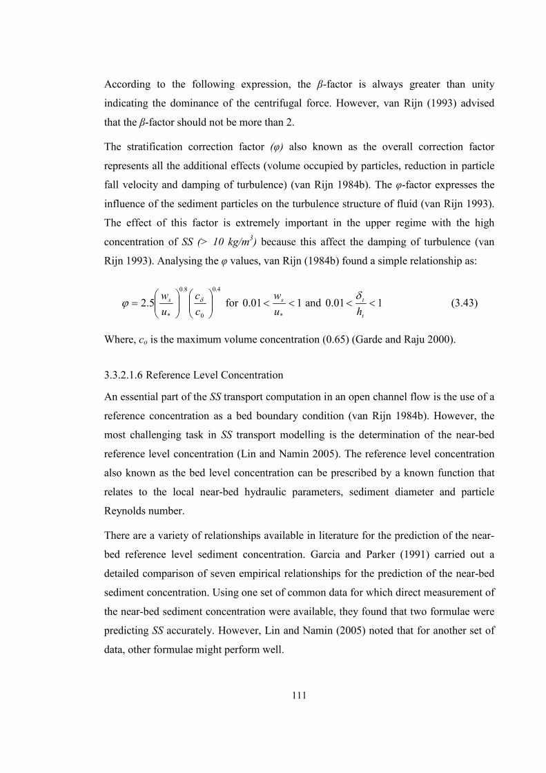
111

According to the following expression, the β-factor is always greater than unity

indicating the dominance of the centrifugal force. However, van Rijn (1993) advised

that the β-factor should not be more than 2.

The stratification correction factor (φ) also known as the overall correction factor

represents all the additional effects (volume occupied by particles, reduction in particle

fall velocity and damping of turbulence) (van Rijn 1984b). The φ-factor expresses the

influence of the sediment particles on the turbulence structure of fluid (van Rijn 1993).

The effect of this factor is extremely important in the upper regime with the high

concentration of SS (> 10 kg/m3) because this affect the damping of turbulence (van

Rijn 1993). Analysing the φ values, van Rijn (1984b) found a simple relationship as:

4.0

0

8.0

*

5.2

=

cc

uws δϕ for 101.0

*

<<uws and 101.0 <<

t

t

hδ

(3.43)

Where, co is the maximum volume concentration (0.65) (Garde and Raju 2000).

3.3.2.1.6 Reference Level Concentration

An essential part of the SS transport computation in an open channel flow is the use of a

reference concentration as a bed boundary condition (van Rijn 1984b). However, the

most challenging task in SS transport modelling is the determination of the near-bed

reference level concentration (Lin and Namin 2005). The reference level concentration

also known as the bed level concentration can be prescribed by a known function that

relates to the local near-bed hydraulic parameters, sediment diameter and particle

Reynolds number.

There are a variety of relationships available in literature for the prediction of the near-

bed reference level sediment concentration. Garcia and Parker (1991) carried out a

detailed comparison of seven empirical relationships for the prediction of the near-bed

sediment concentration. Using one set of common data for which direct measurement of

the near-bed sediment concentration were available, they found that two formulae were

predicting SS accurately. However, Lin and Namin (2005) noted that for another set of

data, other formulae might perform well.

112

For this research project, the basic idea for the calculation of the SS concentration at the

reference level was gained from the research study conducted by van Rijn (1984a,

1984b). The concentration of SS at the reference level was demonstrated in terms of the

particle characteristics as follows:

( ) 2.0

5.150000015.0

ep

t

tta R

TDc ⋅=

δ (3.44)

Where, D50 is the median particle diameter of SS (m) which is determined from the field

measurements of SS particles, Tt is the bed shear (transport stage) parameter

(dimensionless) at time ‘t’ and Rep is the particle Reynolds number.

3.3.2.1.7 Bed-shear Stress Parameter

For the determination of the reference level SS concentration using Equation 3.44, it is

necessary to calculate the bed-shear stress parameter (Tt). The developed model

employed the van Rijn’s (1993) equation for the calculation of the bed-shear stress

parameter. The expression can be written as follows:

( )crb

crbtbtT

,

,/

τττ −

= (3.45)

Where, ( )tb/τ is the current related effective bed-shear stress (N/m2) at time ‘t’ and crb,τ

is the critical time averaged bed-shear stress (N/m2) according to Shields.

The current related effective bed-shear stress was determined as a function of grain

friction efficiency and grain related bed-shear stress. The mathematical expression can

be written as:

( ) ( )tbttb τητ =/ (3.46)

Where, ( )tbτ is the grain related bed-shear stress at time ‘t’ and tη is the grain friction

efficiency which is determined from the ratio of the current related Chezy coefficient to

the grain related Chezy coefficient and determined as follows:

( )2/ttt CC=η (3.47)

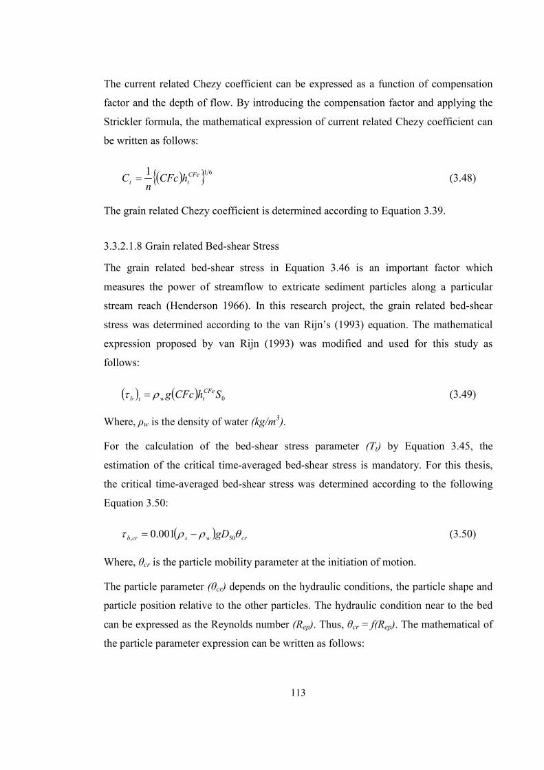
113

The current related Chezy coefficient can be expressed as a function of compensation

factor and the depth of flow. By introducing the compensation factor and applying the

Strickler formula, the mathematical expression of current related Chezy coefficient can

be written as follows:

( ){ } 611 CFett hCFc

nC = (3.48)

The grain related Chezy coefficient is determined according to Equation 3.39.

3.3.2.1.8 Grain related Bed-shear Stress

The grain related bed-shear stress in Equation 3.46 is an important factor which

measures the power of streamflow to extricate sediment particles along a particular

stream reach (Henderson 1966). In this research project, the grain related bed-shear

stress was determined according to the van Rijn’s (1993) equation. The mathematical

expression proposed by van Rijn (1993) was modified and used for this study as

follows:

( ) ( ) 0ShCFcg CFetwtb ρτ = (3.49)

Where, ρw is the density of water (kg/m3).

For the calculation of the bed-shear stress parameter (Tt) by Equation 3.45, the

estimation of the critical time-averaged bed-shear stress is mandatory. For this thesis,

the critical time-averaged bed-shear stress was determined according to the following

Equation 3.50:

( ) crwscrb gD θρρτ 50, 001.0 −= (3.50)

Where, θcr is the particle mobility parameter at the initiation of motion.

The particle parameter (θcr) depends on the hydraulic conditions, the particle shape and

particle position relative to the other particles. The hydraulic condition near to the bed

can be expressed as the Reynolds number (Rep). Thus, θcr = f(Rep). The mathematical of

the particle parameter expression can be written as follows:

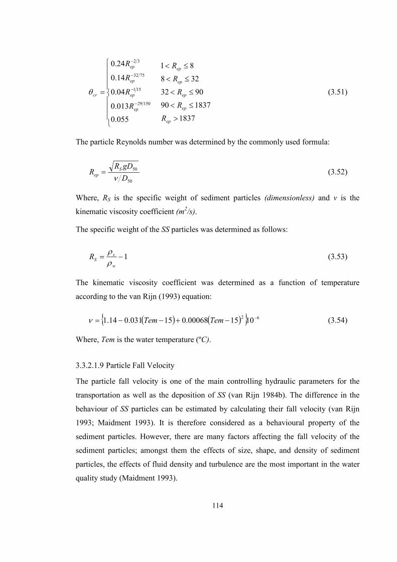
114

=−

−

−

−

055.0

013.0

04.0

14.0

24.0

15029

151

7532

32

ep

ep

ep

ep

cr

R

R

R

R

θ

1837

183790

9032

328

81

>

≤<

≤<

≤<

≤<

ep

ep

ep

ep

ep

RRR

RR

(3.51)

The particle Reynolds number was determined by the commonly used formula:

50

50

DgDR

R Sep ν= (3.52)

Where, RS is the specific weight of sediment particles (dimensionless) and ν is the

kinematic viscosity coefficient (m2/s).

The specific weight of the SS particles was determined as follows:

1−=w

sSR

ρρ (3.53)

The kinematic viscosity coefficient was determined as a function of temperature

according to the van Rijn (1993) equation:

( ) ( ){ } 62 101500068.015031.014.1 −−+−−= TemTemν (3.54)

Where, Tem is the water temperature (ºC).

3.3.2.1.9 Particle Fall Velocity

The particle fall velocity is one of the main controlling hydraulic parameters for the

transportation as well as the deposition of SS (van Rijn 1984b). The difference in the

behaviour of SS particles can be estimated by calculating their fall velocity (van Rijn

1993; Maidment 1993). It is therefore considered as a behavioural property of the

sediment particles. However, there are many factors affecting the fall velocity of the

sediment particles; amongst them the effects of size, shape, and density of sediment

particles, the effects of fluid density and turbulence are the most important in the water

quality study (Maidment 1993).

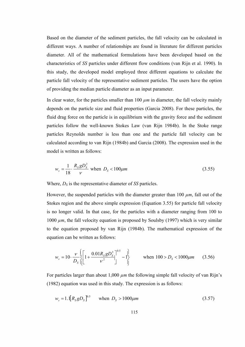
115

Based on the diameter of the sediment particles, the fall velocity can be calculated in

different ways. A number of relationships are found in literature for different particles

diameter. All of the mathematical formulations have been developed based on the

characteristics of SS particles under different flow conditions (van Rijn et al. 1990). In

this study, the developed model employed three different equations to calculate the

particle fall velocity of the representative sediment particles. The users have the option

of providing the median particle diameter as an input parameter.

In clear water, for the particles smaller than 100 µm in diameter, the fall velocity mainly

depends on the particle size and fluid properties (Garcia 2008). For these particles, the

fluid drag force on the particle is in equilibrium with the gravity force and the sediment

particles follow the well-known Stokes Law (van Rijn 1984b). In the Stoke range

particles Reynolds number is less than one and the particle fall velocity can be

calculated according to van Rijn (1984b) and Garcia (2008). The expression used in the

model is written as follows:

ν

2

181 SS

sgDR

w ⋅= when mDS µ100< (3.55)

Where, DS is the representative diameter of SS particles.

However, the suspended particles with the diameter greater than 100 µm, fall out of the

Stokes region and the above simple expression (Equation 3.55) for particle fall velocity

is no longer valid. In that case, for the particles with a diameter ranging from 100 to

1000 µm, the fall velocity equation is proposed by Soulsby (1997) which is very similar

to the equation proposed by van Rijn (1984b). The mathematical expression of the

equation can be written as follows:

−

+⋅= 1

01.0110

5.0

2

3

νν SS

Ss

gDRD

w when mDS µ1000100 <> (3.56)

For particles larger than about 1,000 µm the following simple fall velocity of van Rijn’s

(1982) equation was used in this study. The expression is as follows:

[ ] 5.01.1 SSs gDRw = when mDS µ1000> (3.57)

116

3.3.2.2 Dissolved Oxygen

Dissolved oxygen (DO) is the most important parameter observed in stream water. It

represents the amount of molecular oxygen dissolved in water which is essential for the

plant or animal processes. The prolonged periods of oxygen depletion can results in the

death of fish or other animals; while too much oxygen is a sign of increased plant/algal

biomass due to the nutrients enrichment.

Since DO is the primary reason for the deterioration of the quality of stream water, its

inclusion in stream water quality modelling is crucially important (Bowie et al. 1985).

During storm events, algal activity is negligible for relatively shallow and small streams

(Mannina and Viviani 2010). Therefore, the contribution of DO due to algal biomass

can be avoided throughout rainfall events. Since this study is concentrated on the

pollutant transportation during rainfall events for relatively shallow streams, it can be

assumed that there is the saturation level of DO in a stream.

The most frequently used method for the estimation of saturated DO is the polynomial

equation developed by Elmore and Hayes (1960) for distilled water (Bowie et al. 1985).

Elmore and Hayes (1960) have summarised the works of different researchers who

measured DO at the saturation level. All of these equations were developed as functions

of the temperature. Using the method of Elmore and Hayes (1960), the DO model of the

stream water quality model is presented as follows:

( ) ( )32 00077774.00079910.041022.0652.14 TemTemTemDODO sat −+−== (3.58)

Where, DO is the concentration of the dissolved oxygen and DOsat is the concentration

of DO at the saturation level.

3.3.2.3 Biochemical Oxygen Demand

Biochemical oxygen demand (BOD) is a measure for determining the amount of oxygen

required by aerobic biological organisms in a water body for the decomposition of

organic matter at a certain temperature over a specific time period. It is the most

important parameter which controls the quality of water. Therefore, the estimation of

BOD is most important in water quality modelling.

117

Usually, the processes of BOD decay are described by assuming first order kinematics.

These processes are well-recognised and widely employed approaches in the estimation

of BOD for stream water. Although these techniques are widely used as an organic

quality of water, they are empirical methods. In this research project, the main equation

employed for the simulation of the BOD decay rate can be expressed according to

Equation 3.59 as follows:

( ){ }[ ]tout

tkkkttin

t QeBODQ

BODudsusBODsBODBOD

_

1_ 1 ∆−+−− −

= (3.59)

Where, BODt is the concentration of BOD at time ‘t’, BODt-1 is the concentration of

BOD at time t-1, kBOD is the rate of oxidation of BOD (i.e. BOD decay rate) (1/day),

ksBOD is the rate of BOD loss due to settling (1/day), ksusBOD is the re-suspension rate of

BOD (1/day), Δtud is the time taken for a pollutant to reach from the upstream to the

downstream of a stream reach section (day), Qin_t is the inflow discharge at time ‘t’

(m3/s) and Qout_t is the outflow discharge at time ‘t’ (m3/s).

In a column of water, the BOD decay rate is influenced by a number of factors. The

influences of these factors are described by using the both theoretical and empirical

formulations. Amongst the factors which influence the BOD decay rate, the temperature

is the most important (Bowie et al. 1985). The BOD decay rate occurs at a rate, which

increases with the increasing temperature up to the point, where protein denaturation

begins. Therefore, Equation 3.59 of BOD decay rate should be modified for the

inclusion of the temperature effects. The following mathematical expression of

Equation 3.60 was used in the current model development to simulate the temperature

effects of BOD.

DODOkk

BOD

TeBODBODTeBOD +

⋅= −

δθ 20

)20()( (3.60)

Where, kBOD(Te) is the rate of oxidation of BOD at (Te) °C temperature, kBOD(20) is the rate

of oxidation of BOD at temperature 20 °C, θBOD is the temperature correction factor for

the organic decay and δBOD is the half saturation constant for BOD decay.

118

3.3.2.4 Total Nitrogen

Since nutrients availability is one of the main factors in controlling algal bloom, the

nutrients dynamics are essential in any water quality model (Bowie et al. 1985). For the

development of proper watershed management strategies, information on the

mechanisms of nutrients mobilisation into waterways and water bodies is essential

(Mathers et al. 2007).

Bowie et al. (1985) noted that in a stream system, the nitrogen dynamics are modelled

in complex manner; because of their substantial biogeochemical role, important

oxidation-reduction reactions and other important water quality variables. In natural

water, the denitrification process reduces the amount of TN. On the other hand, the

mineralisation of BOD by the bacteria releases TN in the water. Again, the settling of SS

reduces the amount of adsorbed TN in the stream processes. In this study, three major

processes were employed in the development of the TN model, i.e. denitrification,

mineralisation from BOD and sedimentation. Rusjan et al. (2008) found that the

concentration of nitrogen in rainfall is less; and hence the atmospheric input of nitrogen

to rainwater is significant. Therefore, it is not included in the current modelling.

All the processes of TN that occur in a stream reach are described assuming the first

order kinematics. The governing equation for the transformation of TN employed in the

model is described as follows:

( ){ }tout

SETsTNtk

tTNtk

ttint Q

SSkeBODkeTNQTN

udBODudDEN

_

11_ 1 −+−=

∆−−

∆−− (3.61)

Where, TNt is the concentration of TN (mg/l) at time ‘t’, TNt-1 is the concentration of TN

(mg/l) at time t-1, kDEN is the denitrification coefficient of TN (1/day), kTN is the

coefficient for the mineralisation of TN from BOD, ksTN is the release rate of TN from

sediment and SSSET is the SS which settles on the bottom.

The temperature influences the rate parameters of all nitrogen transformation processes.

Therefore, all of the rate coefficients are temperature dependent. A reference

temperature of 20 °C is usually assumed when specifying each rate coefficient (Bowie

et al. 1985). The governing equations for the temperature correction factor are described

as follows:

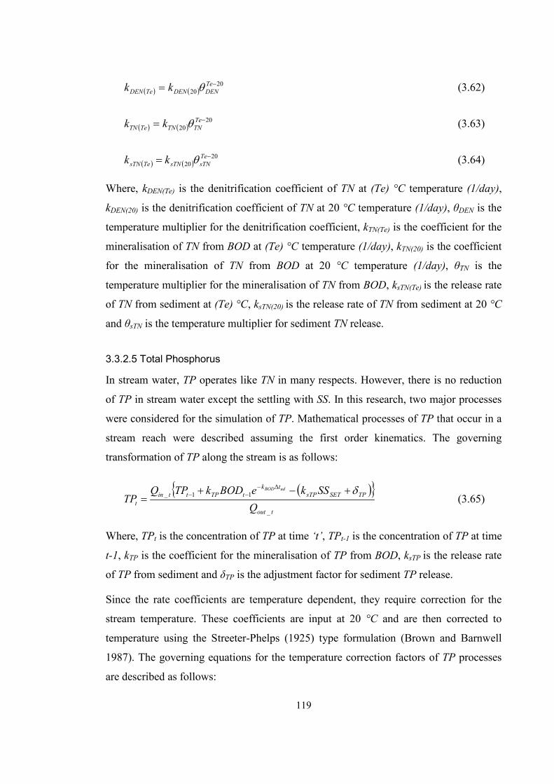
119

( ) ( )20

20−= Te

DENDENTeDEN kk θ (3.62)

( ) ( )20

20−= Te

TNTNTeTN kk θ (3.63)

( ) ( )20

20−= Te

sTNsTNTesTN kk θ (3.64)

Where, kDEN(Te) is the denitrification coefficient of TN at (Te) °C temperature (1/day),

kDEN(20) is the denitrification coefficient of TN at 20 °C temperature (1/day), θDEN is the

temperature multiplier for the denitrification coefficient, kTN(Te) is the coefficient for the

mineralisation of TN from BOD at (Te) °C temperature (1/day), kTN(20) is the coefficient

for the mineralisation of TN from BOD at 20 °C temperature (1/day), θTN is the

temperature multiplier for the mineralisation of TN from BOD, ksTN(Te) is the release rate

of TN from sediment at (Te) °C, ksTN(20) is the release rate of TN from sediment at 20 °C

and θsTN is the temperature multiplier for sediment TN release.

3.3.2.5 Total Phosphorus

In stream water, TP operates like TN in many respects. However, there is no reduction

of TP in stream water except the settling with SS. In this research, two major processes

were considered for the simulation of TP. Mathematical processes of TP that occur in a

stream reach were described assuming the first order kinematics. The governing

transformation of TP along the stream is as follows:

( ){ }tout

TPSETsTPtk

tTPttint Q

SSkeBODkTPQTP

udBOD

_

11_ δ+−+=

∆−−− (3.65)

Where, TPt is the concentration of TP at time ‘t’, TPt-1 is the concentration of TP at time

t-1, kTP is the coefficient for the mineralisation of TP from BOD, ksTP is the release rate

of TP from sediment and δTP is the adjustment factor for sediment TP release.

Since the rate coefficients are temperature dependent, they require correction for the

stream temperature. These coefficients are input at 20 °C and are then corrected to

temperature using the Streeter-Phelps (1925) type formulation (Brown and Barnwell

1987). The governing equations for the temperature correction factors of TP processes

are described as follows:

120

( ) ( )20

20−= Te

TPTPTeTP kk θ (3.66)

( ) ( )20

20−= Te

sTPsTPTesTP kk θ (3.67)

Where, kTP(Te) is the coefficient for the mineralisation of TP from BOD at (Te) °C, kTP(20)

is the coefficient for the mineralisation of TP from BOD at 20 °C, θTP is the temperature

multiplier for the mineralisation of TP from BOD, ksTP(Te) is the release rate of TP from

sediment at (Te) °C, ksTP(20) is the release rate of TP from sediment at 20 °C and θsTP is

the non-dimensional temperature multiplier for sediment TP release.

3.4 Integration of the Models The need for the integrated assessment and modelling has grown extensively as the

severity of environmental problems in the 21st Century worsens and to meet the

challenges of sustainability. The potential benefits of mathematically predicting and

analysing water quality parameters through the integrated modelling concept are widely

recognised because of the time and cost effectiveness as well as the improved

performance and understanding of the actual behaviour of the whole system. Therefore,

the main objective of this thesis was to improve understanding of the tools and water

quality parameters for integrated management of aquatic ecosystems of waterways and

receiving water bodies.

In the literature review, the rationale of the need for the integrated modelling approach

and the general consideration of practices through integrated management were

discussed. However, the review lacks a detailed argument of how one can put the

integrated modelling approach into practice. Risbey et al. (1996) noted that there are a

variety of integrated models which contain a variety of structures. Many of these

structures share a number of core approaches, assumptions, or component models,

which are based on earlier models or pioneer works.

There was no formal equation for the integrated catchment-stream water quantity and

quality simulation. However, it was well recognised that water quality pollutants of a

particular catchment transfers to a stream through the catchment outlet via surface

runoff. Therefore, in this study, the catchment water quality model and the stream water

quality model were developed individually.

121

The models of the subsystems were formulated in a consistent way and run in parallel to

consider the interactions in both ways or to use information from the downstream

system to take control actions in the upstream system. Finally, both of the models were

integrated to be able to continuously simulate the mentioned water quality parameters.

The output from the catchment water quality model was used as the input for the stream

water quality model. In each case, the integration was proposed as a means to overcome

the separation and fragmentation.

Manual calculation of runoff and pollutant loads is time consuming and expensive.

Therefore, a computer program was developed by the author for the formulation of the

catchment and stream water quality models and their integration. The modelling codes

were developed by using the Visual Basic 6.0. The source code is not included with this

thesis to reduce the volume.

3.5 Conclusions Due to the multiplicity of water quality constituents, the quality of natural water varies

in time and among locations. The high cost of water quality samples collection from

every location and their laboratory analysis is the greatest hindrance in monitoring water

quality at the field level. Therefore, water quality modelling plays an important role for

the assessment of physical, chemical and biological changes in waterways and receiving

water bodies. However, the need for the integrated modelling approach has become

prevalent over recent years as decision makers feel dissatisfied with the results from

‘narrowly-focused’ isolated models. The integrated modelling approach recognises the

complexity of the natural systems and their interactions. This approach further provides

a better control of pollutant build-up and wash-off from catchment surfaces.

This chapter has described the development of an integrated catchment-stream water

quality model which continuously simulates different water quality parameters. The

integrated model is capable for simulating both single event and continuous runoff and

pollutant loads. To develop an integrated water quality model, it was necessary to obtain

an improved understanding of the relevant models. Therefore, the integrated model

comprised of two individual models, i.e. the catchment water quality model and the

stream water quality model.

122

Considering the TA method, a rainfall-runoff model was developed. Then processes of

water quality parameters were incorporated with the rainfall-runoff model which

represents the catchment water quality model. Water quality parameters of catchments

transfer to a stream through the catchment outlet with surface runoff and are discharged

into receiving water bodies. Therefore, a stream water quality model was developed

with the same water quality parameters of the catchment water quality model. However,

for the stream water quality model, the process of BOD was also included. Finally, the

catchment water quality model and the stream water quality model were integrated for

the continuous simulation of the mentioned water quality parameters.

The model was developed to create a scientific and technical base from which

standardised integrated catchment-stream water quality modelling can be established.

The model provides a mathematical framework for the phenomena occurring during the

td and storm event to catchment surfaces. The equations represent the dominant

processes affecting water quality parameters but include empirical terms and

coefficients. The model algorithms are based on the known performance characteristics

of common stormwater quality improvement measures.

The major advantage of the model is the continuous simulation of water quality

parameters by an integrated modelling approach. The integrated model eliminates the

inconsistent results which arise from isolated models. The model will help to avoid the

split responsibilities for management and planning of catchments and streams, and can

be used for mixed land-use areas. The model can be used to extend water quality

surveillance and to predict the future water quality/quantity conditions.

The developed model has the potential to give the reliable prediction results of water

quality parameters under the practical and complex conditions. The preparation process

of the input data for the model is simple. The capability of the model to simulate surface

runoff from a wide range of intensities make the model useful to assess the impact of

water quality parameters to waterways and receiving water bodies and to the design

effective stormwater treatment measures.

123

Chapter 4 Data Collection and Study Catchments

4.1 Background It is well recognised that the prediction of water quality parameters for the purpose of

watershed management strategies rely on the mathematical modelling output. Water

quality models are important for understanding and explaining the pollutants processes

and predicting the impact of the future changes (such as environmental policy) on water

resources (Glavan et al. 2011). However, the application of any water quality model

depends on calibration and validation with sufficient and reliable field data (Bouteligier

et al. 2002). The need for data on background or base-line conditions is the essential

requirements for watershed management strategies. All of the empirical equations of

any model should be calibrated and validated against adequate data. Water quality

predictions through any surface runoff model are useless without local data. Due to the

lack of local data for calibration of any water quality model leads to the significantly

biased results for the precise estimation of pollutant loads.

The quality of water in any drainage area depends on the land-use of that particular area.

According to Chen and Adams (2006), the water quality model parameters vary not

only spatially (i.e. catchment to catchment), but also temporally (i.e. differ among

different rainfall events). Although SWMM is used in many countries, Leinster and

Walden (1999) discouraged the generic application of water quality models not only

from overseas countries but also from other parts of the same country. Tsihrintzis and

Hamid (1998) noted that due to the absence of measured data, water quality models

calibrated for other similar sites can be used only for screening purposes. Because

depending upon the catchment characteristics (permeability of soils, initial pollutant

loads), the impact of the actual land-use and management changes (Volk et al. 2009).

Therefore, Puckett (1995) noted that watershed management plan needs to be developed

based on individual watershed information.

124

This chapter of the thesis demonstrates the description of necessary data and the

catchment characteristics which were used as case study for this research. The

description has a particular focus on the characteristics of the physical environment that

influence the quality of water. The primary focus was to obtain both water quantity and

quality data which were observed at the catchment outlet. Water quality data collection

was performed in two stages, i.e. the experimental data collection and the observed field

data collection. The experimental data were collected from published literature. The

measured field data were collected from GCCC, Australia. The experimental

catchments were only impervious and the observed catchments were mixed land-uses.

4.2 Data Requirements for the Model Since the developed model is comprised of many empirical equations, they need to be

calibrated and validated against sufficient and reliable observed data. The integrated

model was developed by comprising two individual models. Therefore, depending upon

the choice of the users, the data requirements of the integrated model are different.

Specifically, the model requires data for both the catchment water quality model and for

the stream water quality model. Overall, the model requires hydrologic, hydraulic and

water quality data.

For the calibration of the hydrologic component of the catchment water quality model,

precipitation data is perquisite. During a storm event, rainfall undergoes the Evp loss

(mentioned in the literature review). The Evp loss also occurs from surface water of the

uncovered land surfaces. Hence, the model requires Evp data to account this loss.

Moreover, the model needs data for the calculation of IL and CL parameters. Finally,

the model needs the catchment characteristics data. If there is more than one catchment

contributing to surface runoff, the model needs lag time for each of the catchments. For

calibration of the quality component of the catchment water quality model, the

integrated model requires observed water quality data which are collected at the

catchment outlet. All the mandatory information is given as the input parameters during

the runtime of the model. The stream water quality model can be used either as a

separate model or integrated with the catchment water quality model. For both cases,

the stream water quality model needs hydraulic data, initial streamflow data and water

quality data.

125

4.3 Data Collection Good quality hydrologic, pollutants and physical data are required for the calibration

and estimation of the water quality model parameters (Marsden et al. 1973). According

to Boorman (2003), specifying water quality parameters to be modelled without fully

understanding data availability is clearly a weakness in a study that has no data

collection program. Due to the complex nature of pollutants processes, significant array

of data is required for calibration and validation of any water quality model. Moreover,

sufficient and reliable data are essential for improving existing models and creating a

new one (Bertrand-Krajewski et al. 1993).

However, available and reliable data collection is the major challenge in water quality

study (Nicholas and Walling 1998). It was understood that water quality data are not

readily available. Because in most of the cases, data are inadequate and fragmented; and

this put potentially severe limitations to the sustainable management of the nation’s

water (Smith 1998). Zoppou (2001) and Rauch et al. (2002) argued that the lack of data

is the greater hindrance for the development of water quality model than the lack of

suitable algorithms. Due to the scarcity of measured data, the calibration and parameters

estimation are impossible even for the simplest water quality model (Gaume et al.

1998).

In Australia, limited water quality data are available for the calibration and parameters

estimation of sophisticated water quality model (Leinster and Walden 1999). There are

also lots of deficiencies for the currently available data. Deletic and Maksimovic (1998)

identified the common deficiencies of the currently available water quality data. The

major paucity of available water quality data are:

Water quality data on complete storms are very rare.

The capacity of the samplers is limited to collect continuous data throughout

storm events.

Data is recorded at inadequate intervals and the frequency of data collection is

generally low.

Data is usually collected at the outlet of watershed area.

Data is not always reliable.

126

4.3.1 Precipitation Data

For all hydrologic and water quality systems, precipitation data is the key information

because it activates watershed responses in hydrologic systems (Chaubey et al. 1999;

Newham 2002). In this study, one of the major purposes of precipitation data collection

was to calibrate the developed catchment water quality model for the estimation of

surface runoff and to determine the td. Therefore, it was necessary to collect continuous

rainfall hyetographs for a long period of time. Both rainfall simulator data and natural

precipitation data were collected in this research.

Experimental precipitation data of this study was collected from available literature.

Egodawatta (2007) performed experimental study to observe the transferred water

quality parameters from impervious catchment surfaces by using simulated rainfall.

These rainfall simulator data was collected and used for this research project. For the

estimation of the model parameters from the observed water quality data, actual hourly

precipitation data for 2004 - 2008 was used from a nearby rainfall station of the study

catchments. Precipitation data was measured by the weather station ‘Gold Coast

Seaway’ (station no. 40764). Historical rainfall data for the study catchments were

supplied by the Bureau of Meteorology (BoM). Duration of the simulation period and

the number of storm events used in the simulation is shown in Table 4.1. Only those

storm events were selected for the simulation for which water quality measurements

were conducted. As the research project was intended to estimate the amount of

pollutants transferred during storm events, rainfall data was chosen when the water

quality measurement was undertaken.

Table 4.1: Description of storms used in the water quality simulation

Storm No. Duration date No. of

Events

1 10/01/2004 – 19/01/2004 4

2 02/02/2007 – 15/02/2007 6

3 04/07/2008 – 09/07/2008 2

4 04/12/2004 – 06/12/2004 2

5 21/04/2005 – 04/05/2005 5

127

4.3.2 Experimental Water Quality Data

For the estimation of the model parameters from the experimental data, small

impervious catchments from Gold Coast, Australia were selected. The experimental

data obtained by Egodawatta (2007) was used to determine the build-up and wash-off

models parameters from impervious surfaces. The experimental study was done only for

impervious surfaces using simulated rainfall. These data on defined and limited surfaces

were selected to obtain more specific and detailed knowledge on pollutant processes

suggested by other researchers, e.g. Herngren et al. (2005); Vaze and Chiew (2002). The

data was collected from road and roof surfaces.

4.3.3 Observed Water Quality Data

Water quality data collection programs have been initiated in Queensland by a number

of local authorities (Leinster and Walden 1999):

Brisbane City Council

Cairns City Council

Ipswich City Council and

Gold Coast City Council

The observed water quality data used for this research was collected from Gold Coast

City Council (GCCC), Australia. To investigate specific pressures on the health and

environmental quality to nearby waterways and receiving water bodies, runoff water

quality monitoring programs was started by GCCC. Water quality monitoring data

observed by GCCC were studied to obtain insight to the nature of water quality

parameters accumulation and washed-off, and to help improving the long-term

continuous simulation of the catchment water quality model. The same data was also

used for calibration and validation of the stream water quality model.

GCCC has been monitoring water quality parameters at different locations within

catchments. Details of the data monitoring program are contained in the CMU (2002)

report. The observed field data was collected for pervious dominated and mixed

surfaces catchments. For this thesis, water quality data from two different catchments

were used. These catchments were selected after careful consideration where the

detailed water quality monitoring programs were undertaken.

128

It should be noted that for calibration of the catchment water quality model, upper most

sub-catchments were selected to get unaltered pollutants transported only from

catchments, i.e. to avoid water quality samples with pollutant degradation within creek.

The output from the catchment water quality model was used as the input of the stream

water quality model for the integrated simulation of water quality parameters.

4.3.4 Collection of Catchment Characteristics Data

The physical data of the catchment characteristics was collected for the simulation of

the integrated model. These data include catchment areas, percent impervious and

pervious, slopes and roughness parameters. These data were compiled from the several

sources, such as contour maps, aerial photographs and other available literatures.

Generally, every catchment encompasses of two different surface areas, i.e. impervious

surface and pervious surface. Each of the surface area designates different responses to

surface runoff hydrographs and pollutographs. Therefore, any catchment water quality

model requires knowing impervious and pervious surface areas separately. In this study,

the separation was done from percent impervious data. The degree of imperviousness

from the selected catchments was determined from aerial photograph. Pervious surface

area was determined by the model from percent impervious data and represents

differing responses from impervious and pervious surfaces contribution. It was

mentioned earlier that catchment sub-division is important to represent the partial area

contribution for surface runoff quantity and quality. Data for catchment sub-division

was obtained from topographic image maps. If topographic maps were not available,

catchment sub-division data was obtained by using the empirical method of HEC-1.

4.4 Description of the Study Catchments Since the quality of water represents the health of watershed areas, it is important to

monitor watershed conditions to obtain reliable data for the mitigation of water quality

problems (Dai et al. 2004). Tsihrintzis and Hamid (1998) suggested that for the

prediction of water quality parameters with the higher degree of confidence, the site

specific input parameters are mandatory. Therefore, the selection of study area was one

of the most important factors in this study.

129

The Gold Coast area was chosen to collect both experimental and field observation

water quality data. This area is one of the few places in Australia where a

comprehensive catchment monitoring program has been established. Gold Coast is

called the capital of Queensland, Australia. The city is located in the south-east

Queensland, about 78 km south of the Brisbane. The Gold Coast City is bounded by

Logan city, Redland city and Moreton Bay in the north, Coral Sea in the east, the New

South Wales border in the south and the Scenic Rim Region in the west. A location map

of the Gold Coast area is shown in Figure 4.1.

Figure 4.1: Location map of the Gold Coast (GCCC-Web 2010)

Gold Coast is the sixth largest city of Australia. The total area of the city is about 1,406

km2, featuring 40 km of coast line. Based on the city’s estimated resident population,

GCCC is Australia’s second largest local government. The population of the city is

approximately 515,157 and is expected to reach about 600,000 in 2021. Gold Coast is

one of the most famous tourist spots in Australia with approximately 12% of the

population being visitors. There are seven tourist parks and camping ground in the city.

130

Gold Coast has the largest government park estate in Australia and encompasses more

than 2,254 parks covering 22,071 ha of land. There are more than 3,500 ha open spaces

for sports and recreation. Beaches and waterways in particular are most important

tourist attractions (GCCC-Web 2010).

Gold Coast city has a sub-tropical climate with average 287 days of sunshine annually.

The city is with moderate temperature and summer dominated precipitation. The

average temperature in summer ranges from 19 °C to 29 °C (66 to 83 degrees

Fahrenheit) and winter temperature ranges from 9 °C to 21 °C (48 to 69 degrees

Fahrenheit). The city’s stormwater drainage system features many natural and artificial

waterways. These waterways include the five major rivers and numerous creeks, many

of which are connected to artificial lakes and canals. Total length of rivers and streams

run through the city is about 480 km. Navigable waterways of the city are around 260

km which is 9 times more than the Venice. Wetland reserves, lakes, dams and canals are

more than 1,000 ha. The major watershed basins of the city are shown in Figure 4.2.

Figure 4.2: Major watershed basins of Gold Coast city (GCCC)

131

The waterways of the Gold Coast city flow from the surrounding west ward hilly area

towards the Pacific Ocean coastline. Natural vegetation occupies a significant fraction

of the regional land particularly west of the city. High density urban areas are located

close to the coastline. Most of the residential settlements have developed adjacent to the

city’s integrated waterways which promote luxurious waterside living. There are about

3,139 km of roads, more than 600 km of bikeways, and 923 km of paths and walkways

in the Gold Coast city. The city has a protected natural area more than 25,000 ha.

However, extensive urban development alongside the different waterways of the city

influences the key environmental values of waterways ecology (GCCC-Web 2010).

4.4.1 Description of the Experimental Catchments

To investigate pollutants build-up and wash-off, Egodawatta (2007) conducted

experimental study on the two different types of impervious surfaces, i.e. road and roof

surfaces for SS. For the accumulation of pollutant on catchment surfaces, the only

variable considered was the td; while for the wash-off investigation, rainfall intensity

and duration was considered. The area of all experimental catchments (road and roof

surfaces) remained the same, i.e. 3 m2.

4.4.1.1 Road Surfaces Catchments

Along the many catchments monitored by GCCC, Egodawatta (2007) performed his

experimental study within Highland Park area, Gold Coast, Australia, to investigate

pollutant build-up and wash-off on road surfaces. Highland Park area is predominantly a

residential area, and the area is situated within the boundary of the Nerang River

catchment. The experimental study was performed to the three small road surfaces at:

(a) Lauder Court, (b) Gumbeel Court and (c) Piccadilly Place. Road sections were

straight, about 50 m in length, mild slope with various traffic volumes. Most of the

roads were access road and mainly used by the local traffics. The selected road sections

were wide enough so that the local traffic was not affected during the experimental

period. The roads were in good conditions (Egodawatta 2007). However, there were

ongoing construction activities to the upstream portion of the catchments. The

characteristics summaries of road surface catchments are shown in Table 4.2.

132

Table 4.2: Characteristics summary of the road surfaces catchments (Egodawatta 2007)

Site Description Slope

(%)

Surface texture

depth (mm)

Number of

households

Area

(m2)

Lauder Court Single detached

housing area

10.00 0.66 12 3

Gumbeel Court Duplex housing area 7.20 0.92 25 3

Piccadilly

Place

Single detached

housing area

10.80 0.83 41 3

4.4.1.2 Roof Surfaces Catchments

For the experimental study of pollutant build-up and wash-off processes on roof

surfaces, Egodawatta (2007) selected the two roof materials at Southport Deport, Gold

Coast, Australia. The two roofing materials used in the experimental study were: (a)

corrugated steel and (b) concrete tile. The roofing materials selection was done so that

they were representative for the study region. The two study models for the roofs were

designed at an angle of 20°. To reduce the human influence and traffic induced

turbulence, roofs were kept at a typical single story roofing height. The maximum

height of the roofs was 2.5 m. Surrounding land-uses of the experimental sites were

commercial and residential (Egodawatta 2007).

4.4.2 Description of the Observed Catchments

The catchment studied in this research work for the collection of observed water quality

data are also located at Gold Coast, Australia. The two catchments were selected as case

study: (a) Hotham creek catchment (HTCC) and (b) Saltwater creek catchment

(SWCC). These two catchments were selected to ensure that different catchment

characteristics and hydraulic systems are represented. As most of the other studies were

based on impervious area, the selected catchments were pervious dominated and mixed.

GCCC is monitoring water quality data for these two catchments. Data from these

catchments were used for calibration of water quality parameters of the developed

integrated model. A detailed map of the creeks running through the study catchments is

shown Figure 4.3.

133

Figure 4.3: Waterways of the Gold Coast City Council

4.4.2.1 Hotham Creek Catchment

Hotham creek is the main tributary of the Pimpama River. It is a small creek with

approximately 15 km in length. The headwater of the creek runs through residential

areas near Willowvale, onto floodplain near the Pimpama River. A map of HTCC

indicating area sub-division is shown in Figure 4.4.

134

Figure 4.4: Location of Hotham Creek Catchment

Table 4.3: Summary of the characteristics of HTCC

Catchment Total Area (ha) Imperviousness

(%)

No. of sub-

catchments

Hotham Creek

Catchment

302.35 2.61 8

Hotham is basically a freshwater creek. In this study, considered portion of the creek

drains water from around 302.35 ha. The surface area of the catchment was pervious

dominated. Land-use of the catchment included sugarcane, pasture, quarry and degraded

wetland (Gavine et al. 2000). The upper portion of the catchment was dominated by

farming practices, including dairy and beef cattle, banana and various other crops. For

these farming activities large area of the upper portion was cleared.

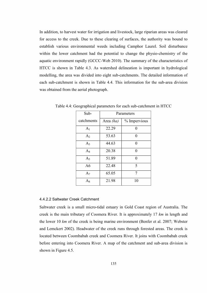
135

In addition, to harvest water for irrigation and livestock, large riparian areas was cleared

for access to the creek. Due to these clearing of surfaces, the authority was bound to

establish various environmental weeds including Camphor Laurel. Soil disturbance

within the lower catchment had the potential to change the physio-chemistry of the

aquatic environment rapidly (GCCC-Web 2010). The summary of the characteristics of

HTCC is shown in Table 4.3. As watershed delineation is important in hydrological

modelling, the area was divided into eight sub-catchments. The detailed information of

each sub-catchment is shown in Table 4.4. This information for the sub-area division

was obtained from the aerial photograph.

Table 4.4: Geographical parameters for each sub-catchment in HTCC

Sub-

catchments

Parameters

Area (ha) % Impervious

A1 22.29 0

A2 53.63 0

A3 44.63 0

A4 20.38 0

A5 51.89 0

A6 22.48 5

A7 65.05 7

A8 21.98 10

4.4.2.2 Saltwater Creek Catchment

Saltwater creek is a small micro-tidal estuary in Gold Coast region of Australia. The

creek is the main tributary of Coomera River. It is approximately 17 km in length and

the lower 10 km of the creek is being marine environment (Benfer et al. 2007; Webster

and Lemckert 2002). Headwater of the creek runs through forested areas. The creek is

located between Coombabah creek and Coomera River. It joins with Coombabah creek

before entering into Coomera River. A map of the catchment and sub-area division is

shown in Figure 4.5.

136

Figure 4.5: Location of the Saltwater Creek Catchment

In this study, considered area of SWCC was approximately 1,025 ha with 33.5%

impervious. The summary characteristics of the catchment are shown in Table 4.5. The

area of the catchment is of varied landscape including virgin bush and housing sub-

divisions. The catchment was significant in social, economic and environmental terms.

The detailed information of each sub-catchment is shown in Table 4.6. Similar to HTCC

these information were derived from aerial photograph.

137

Table 4.5: Summary of the characteristics of SWCC

Catchment Total Area (ha) Imperviousness

(%)

No. of sub-

catchments

Saltwater Creek Catchment 1024.51 33.5 16

Table 4.6: Geographical parameters for each sub-catchment in SWCC

Sub-

Catchments

Parameters

Area (ha) % Impervious

A1 81.15 0

A2 66.77 0

A3 76.92 80

A4 9.75 0

A5 96.01 0

A6 59.26 0

A7 67.11 0

A8 30.62 35

A9 81.06 80

A10 75.65 60

A11 28.49 60

A12 47.82 25

A13 67.35 65

A14 57.79 55

A15 26.96 30

A16 64.06 75

During the study period, the catchment came under the pressure due to the new

development. Residential development was planned within the middle to upper

freshwater region of the catchment with a strong demand for new waterside housing

accommodation. This significant development was placing pressure to the surrounding

water environment due to the various anthropogenic activities (Webster and Lemckert

2002). Hence, SS and nutrients loadings increased for the catchment.

138

4.5 Conclusions In water quality modelling, data is the key information enabling the accurate model

responses. The application of any water quality model always depends on calibration

and validation from adequate and reliable data. Significant array of hydrologic (i.e.

precipitation) and water quality data are required to calibrate and validate any water

quality model. These data may be experimental or measured or both. In addition,

information about the characteristics of the physical environment of a watershed area

which influence the quality of water is essential.

Since equations of the developed integrated model represents water quality processes

and all contain certain degree of empiricism, data are essential for calibration and

validation. Calibration of the model required accurate data of the catchment

characteristics, rainfall-runoff, observed water quality, streamflow and stream water

quality data.

Both the experimental and observed field data were collected from the Gold Coast

region of Australia. The experimental data was collected from the study done by

Egodawatta (2007) for road and roof surfaces using simulated rainfall. The observed

precipitation data was collected from a rainfall station which is very near to the study

catchments. These actual precipitation data for the selected catchments were supplied by

the BoM, Australia. The observed water quality data for the selected catchments were

collected from GCCC, Australia.

The data was collected from two catchments which were pervious dominated and mixed

land-use. The types of issues and physical environments of the study catchments were

generally similar to many other catchments of Australia. Therefore, it was suitable to

adopt water quality data from these catchments for calibration and validation of the

model for the widespread application.

139

Chapter 5 Calibration and Parameters Estimation

5.1 Introduction In order to use any mathematical model for the prediction of water quality parameters, it

is essential to estimate the model parameters which are relevant to modelling processes.

The accuracy of the modelling results largely depends on the accuracy of the model

parameters. Therefore, the parameters estimation is the key step in the practical

application of any water quality model (Karadurmus and Berber 2004).

For all models, the precise prediction of the pollutant concentration and loads rely on an

accurate estimation of the model parameters (Baffaut and Delleur 1990). However, the

estimation of the model parameters is the most critical step in any water quality model

(Tsihrintzis and Hamid 1998). It is often difficult to determine the model parameters

accurately because the values of many model parameters are linked and interrelated to

each other. For example, in the catchment water quality models, the parameters of the

pollutant wash-off model are strongly depended on the pollutant build-up. Due to the

absence of available pollutants on a catchment surface, the wash-off might become zero

even if there is high intensity of rainfall with significant volume of surface runoff. As a

result, there is a possibility in identifying a number of alternative model parameters.

Although it is difficult to estimate the model parameters, they are required for the

analysis, improvement and/or update of existing BMPs (Tsihrintzis and Hamid 1998).

Different researchers use different procedures for the estimation of the model

parameters. For example, Deletic and Maksimovic (1998) and Kim et al. (2006)

proposed indirect methods for the calculation of the model parameters. An alternative

approach is the estimation of the parameters by the calibration procedure using runoff

quality data collected at the watershed outlet (Alley and Smith 1981) which reflects the

combined effects of an entire catchment. Tsihrintzis and Hamid (1998) noted that

calibrated water quality models are essential for specific regions for the prediction of

the impact of different water quality parameters into receiving water bodies.

140

Calibration is an iterative process in which the parameters of a particular model are

constantly adjusted until the deviation or standard error between the simulated and

observed values are minimised to a satisfactory level (Chen and Adams 2007). The

calibration procedure includes the use of the estimated parameters in the field as well as

adjustment of some parameters to match better model predictions with measured data.

The calibration procedure attempts not only to identify the best set of parameters, but

also helps to assess and reduce the uncertainty in parameter values (Beck 1991).

Like any other water quality model, the developed model needs to be correctly

calibrated and verified for a particular catchment before its use for the reliable

prediction of water quality parameters. This chapter of the thesis demonstrates the

estimation of parameters for the developed integrated catchment-stream water quality

model. The main focus was to obtain a set of model parameters for which the predicted

pollutant concentration are close to the measured concentration. The data used to

calibrate the model was collected by runoff sampling. Calibration of the catchment

water quality model and the stream water quality was performed separately for the three

major water quality parameters, i.e. SS, TN and TP. These parameters were selected for

the estimation of the model parameters based on the simulation capability of the

developed model.

5.2 Model Parameters Required Estimation The feasibility of any model depends on its capability of producing the general results

that can be used to aid the implementation of effective management options. Since the

developed model is an integration of a catchment water quality model and a stream

water quality model, it was needed to estimate the parameters for both of the models.

However, each of the models consists of quantity and quality sub-models; and hence the

quantity and quality parameters have to be determined.

For the catchment hydrological model, IL and CL are needed to be determined first. For

the water quality component of the catchment model, it is required to estimate

coefficients and exponents of the pollutant build-up and wash-off models. However, the

phenomena of non-point pollutant build-up and wash-off are influenced by a large

number of factors which make the estimation of the model parameters more difficult

(Temprano et al. 2006).

141

Depending upon the physical characteristics of catchment, the input parameters of

model can vary significantly. Obviously, it is difficult to measure the accurate build-up

and wash-off rates of a particular catchment due to various reasons. Nevertheless, the

application of the developed model requires the proper estimation of the build-up and

wash-off model parameters. Table 5.1 summarises the required model parameters that

needed to be estimated for the catchment water quality model before applying it to a

particular catchment.

Table 5.1: Required parameters for the catchment water quality model simulation

Processes Parameters Symbol Unit

Runoff Initial loss IL mm

Continuing loss ACL, BCL and CCL mm/hr

Pollutant

build-up

Antecedent dry days td day

Maximum build-up rate C1(p,s) kg/km2

Build-up coefficient C2(p,s) 32 Cdaykmkg −⋅

Power of the build-up rate C3(p,s) -

Build-up exponent kp(p,s) 1/day

Half saturation constant tp(p,s) day

Pollutant

Wash-off

Wash-off coefficient E1(p,s) [ ] 2Ehrmm −

Wash-off exponent E2(p,s) -

Wash-off rate coefficient E3(p,s) [ ] 4Esmkg −

Power of wash-off rate E4(p,s) 1/mm-

Wash-off exponent E5(p,s) -

Like the catchment water quality model, it was required to estimate the parameters for

both water quantity and quality sub-models of the stream water quality model. For the

quantity model, hydrologic and hydraulic parameters are to be estimated. For the quality

model, the main processes of SS, TN, TP and BOD were considered and hence the

parameters of relevant processes are to be determined. Table 5.2 lists the number of

parameters required to be estimated for the stream water quality model.

142

Table 5.2: Required parameters for the stream water quality model simulation

Processes Parameters Symbol Unit

Runoff

Reach Length L km

Sub-reach Length ∆L m

Weighing factor XP -

Reach storage parameter Kstor sec

Stage discharge parameters a, b -

Compensation factors CFc, CFe -

Channel bed Slope S0 m/km

Manning’s roughness n -

SS

Water temperature Tem °C

Water density ρw kg/m3

Particle size of incoming SS D50, D90 mm

Density of SS ρs kg/m3

BOD

BOD decay rate kBOD 1/day

BOD settling rate ksBOD 1/day

BOD suspension rate kssBOD 1/day

Temperature correction factor for organic decay θBOD -

Half saturation constant δBOD 1/day

TN

Denitrification coefficient kDEN 1/day

Release rate of TN from BOD kTN 1/day

Release rate of TN from SS ksTN 1/day

Temperature multiplier for the mineralisation of

TN from BOD

θTN -

Temperature multiplier for sediment TN release θsTN -

TP

Release rate of TP from BOD kTP 1/day

Release rate of TN from SS ksTP 1/day

Adjustment factor of sediment TP release δTP -

Temperature multiplier for the mineralisation of

TP from BOD

θTP -

Temperature multiplier for sediment TP release θsTP -

143

5.3 Estimation of Catchment Water Quality Model Parameters Selection of an appropriate set of parameter values of any catchment quality model is

essential to simulate the catchment responses accurately. Since the developed catchment

water quality model consists of a number of functional sub-models, such as rainfall-

runoff transformation, pollutant build-up and wash-off, it was required to calibrate all

these sub-models. Based on available data sets, the catchment water quality model was

calibrated for the selected catchments. The major parameters of runoff, build-up and

wash-off models were adjusted until the deviation or standard error between the

simulated value and the observed value of pollutant loads were reduced to a satisfactory

level.

The estimation of the model parameters was performed from the both experimental and

observed field data. The experimental data was collected from impervious catchments

and the observed data were collected from catchments with mixed (impervious and

pervious) land-uses. The parameters estimation from the experimental data was

performed by using trend lines of fitting data sets. From the available observed field

data, the parameters estimation was done by using the calibration procedure. Where the

observed data was not available, the parameters were estimated from information of

available literature and by comparisons with widely used water quality models. The

estimation of the hydrologic and water quality model parameters was performed

separately.

5.3.1 Hydrologic Model Parameters Estimations

As the output of the runoff model is used as the input of the pollutant model, the

estimation of hydrologic model parameters was performed before the estimation of the

pollutant model parameters. In order to accomplish this hydrologic calibration and

parameters estimation, precipitation records of the ‘Gold Coast Seaway’ station were

analysed. The total five rainfall events ranging from low to high intensity were selected

for the estimation of hydrologic parameters of the developed model. The duration of the

simulation periods and the number of rainfall events simulated is shown in Table 5.3.

Rainfall and evaporation data for the selected dates and catchments were used as the

input parameters for the model.

144

Calibration of the hydrological model was performed for IL, CL parameters and

catchments roughness. The parameters were progressively adjusted within reasonable

limits to improve the model performance. These parameters were estimated for two

selected catchments, i.e. HTCC and SWCC.

Table 5.3: Description of the storms used in this study

Simulation

No.

Duration date No. of

Events

Simulated for

Catchment

1 10/01/2004 – 19/01/2004 4 HTCC

2 02/02/2007 – 15/02/2007 6 HTCC

3 04/07/2008 – 09/07/2008 2 HTCC

4 04/12/2004 – 06/12/2004 2 SWCC

5 21/04/2005 – 04/05/2005 4 SWCC

No runoff measurements for these catchments were conducted during the sampling

period. For this reason, the developed catchment water quality model was calibrated

with the results of WBNM and DRAINS which are widely used models in Australia.

For these models, the values of IL and CL were adopted by reviewing available

literature for similar conditions.

5.3.1.1 Initial Loss and Continuing Loss Model Parameters

Usually, it is considered that IL happen at the very beginning of a rainfall event and it is

considered as constant. However, CL occurs after the commencement of surface runoff

and mainly comprises of infiltration. In the absence of available data, these losses were

determined from information of published literature.

For Australia, the values of rainfall loss can be derived from the Australian Rainfall

Runoff (ARR). In Appendix A, the values of IL and CL are shown for some regions of

Australia. For other regions the values of these losses can be taken from the IEAust

(2001) or can be derived from the experimental studies. In this study, the values of IL

and CL were determined from the suggested typical ranged values of ARR. The

simulation was first performed by using the suggested parameters of IEAust (2001).

145

The simulation results were further improved by varying each parameter so that the

values lie within the ranged values suggested by IEAust (2001). The final adopted

values of rainfall loss parameters are summarised in Table 5.4. Based on the final

adopted parameters, the model simulated hydrographs, the peak discharge and the

duration of runoff for the selected catchments. The summary of the computed peak

discharge and their comparisons with other models (WBNM, DRAINS and Rational

Method) are shown in Tables 5.5 and 5.6 for HTCC and SWCC respectively.

Table 5.4: Final values of the hydrological parameters used in the runoff model

Parameters Surface HTCC SWCC

Initial Loss (mm) IMPV 0 0

PEV 15 15

Continuing loss

(mm/hr)

IMPV 0 0

PEV 2.5 2.5

Evaporation (mm/day) - 24.1 - 27.4 24.6 - 25.7

Table 5.5: Comparison of the peak discharges for HTCC

Events

Date

Peak discharge (m3/s) for HTCC

Rainfall

Intensity

Simulated WBNM DRAINS Rational

Method

1 15/01/2004 32.96 35.29 30.8 27.34 Medium

2 30/08/2005 0.06 0.057 0.06 1.79 Low

3 13/02/2007 104.37 110.77 104 83.16 High

4 08/07/2008 8.77 9.531 6.74 8.98 Low to Medium

Table 5.6: Comparison of the peak discharges for SWCC

Simulation

No.

Date

Peak Discharge (m3/s) Rainfall

Intensity Simulated WBNM DRAINS

1 06/12/2004 64.70 64.706 58.1 High

2 03/05/2005 74.39 74.382 68.3 High

3 19/03/2008 0.95 0.952 0.953 Low

146

The plotted results of the comparisons are shown in Figures 5.1 to 5.4 for HTCC and

Figures 5.5 to 5.7 for SWCC. From Table 5.5 and Figure 5.1, it is clear that the rational

method gave the higher peak discharge for the low intensity rainfall for HTCC. This

was also true for medium intensity rainfall shown in Table 5.5 and Figure 5.2.

Figure 5.1: Peak discharge comparison for low rainfall intensity (HTCC)

Figure 5.2: Peak discharge comparison for medium-low rainfall intensity (HTCC)

147

Figure 5.3: Peak discharge comparison for medium rainfall intensity (HTCC)

Figure 5.4: Peak discharge comparison for high rainfall intensity (HTCC)

On the other hand, for the higher intensity rainfall, the rational method under-estimated

the peak flow as shown in Figures 5.3 and 5.4. This was due to the effects of partial area

contribution considered in the other methods. For low intensity rainfall, the rational

method considered the whole catchment area in estimating the peak discharge which

leads to the estimation of the higher values. For high intensity rainfall, it is doing the

same thing as with average rainfall intensity. The other models consider the partial area

effect with exact rainfall intensity producing the exact peak discharge.

148

From Table 5.6 and Figure 5.5 it can be concluded that for low intensity rainfall, the

simulated peak discharge of the developed model was close to the outcomes of other

models for SWCC. For high intensity rainfall, the simulated peak discharge was also

very much closer to the WBNM simulated peak discharge as shown in Figure 5.7.

However, comparing it with the DRAINS model results, the simulated peak discharge

was little bit higher.

Figure 5.5: Peak discharges comparison for the low intensity rainfall (SWCC)

Figure 5.6: Peak discharges comparison for medium-high intensity rainfall (SWCC)

149

The difference of the simulated results with the WBNM and DRAINS were due to the

sub-division of catchment area. Both the developed model and the WBNM model used

the sub-area divided from the aerial photography. However, the DRAINS model

subdivided the catchment area automatically. Hence, the peak discharge from the

DRAINS model differs from the actual value. Nevertheless, observed discharge

measurements were required to decide suitability of the models for the catchment. Also

the simulated time to the peak of the developed model is similar to the other models

outcomes for all rainfall events. The simulated peak discharges of the developed model

were very close to the peak discharges simulated by other models indicating the

suitability of the model for runoff simulations.

Figure 5.7: Peak discharge comparison for high intensity rainfall (SWCC)

To compare the performance of the developed hydrological model, two error statistics

PBIAS (percent bias) and NSE (Nash Sutcliffe efficiency) were computed. Where,

( ) ∑∑==

−=N

t

obst

N

t

simt

obst QQQPBIAS

11

(5.1)

( ) ( )∑∑==

−−−=N

t

meant

obst

N

t

obst

simt QQQQNSE

1

2

1

21 (5.2)

150

As there was no observed runoff data for the catchment at that time, statistical

comparisons were made with the DRAINS model. The first statistic PBIAS measure is

the average tendency of simulated flows to be larger or smaller than their observed

counterparts. The optimal value is zero; positive values indicate a model bias towards

the underestimation, whereas negative values indicate a bias towards the overestimation

(Gupta et al. 1999). For our data sets, the PBIAS value was 0.00 for low intensity

rainfall and -0.09 to -0.16 for high intensity rainfall.

The second statistic, NSE, provides normalise indicators of model performance in

relation to benchmarks. It measures the relative magnitude of the residual variance to

the variance of flows. The optimum value is 1.0, and the value should be larger than 0.0

to be a ‘minimally acceptable’ performance (Moriasi et al. 2007). A value equal to zero

indicates that the mean observed flow is a better predictor than the model. For our data

sets NSE value was 1.00 for low intensity rainfall and 0.60 to 0.88 for the higher

intensity of rainfall. Again these variations in statistics were due to the different

methods used in the sub-division of the catchment. However, the observed data is

needed to compare the reliability of statistics of the developed model.

5.3.2 Water Quality Model Parameters from Experimental Data

The water quality component of the catchment water quality model requires the

specification of the model parameters for the both pollutant build-up and wash-off

models. The developed model was used to represent the available experimental data

collected from street and roof surfaces from residential catchments at Gold Coast,

Australia. As no experimental data were found for TN and TP, the estimation of the

model parameters was performed only for SS. It was mentioned in Chapter 4 that

Egodawatta (2007) assessed the pollutant build-up and wash-off at Gold Coast, for low

and high population density residential areas from impervious surfaces. The

experimental study was performed on road and roof surfaces using simulated rainfall.

This experimental data collected by Egodawatta (2007) was used to estimate the

parameters of the pollutant build-up and wash-off equations of the developed catchment

water quality model.

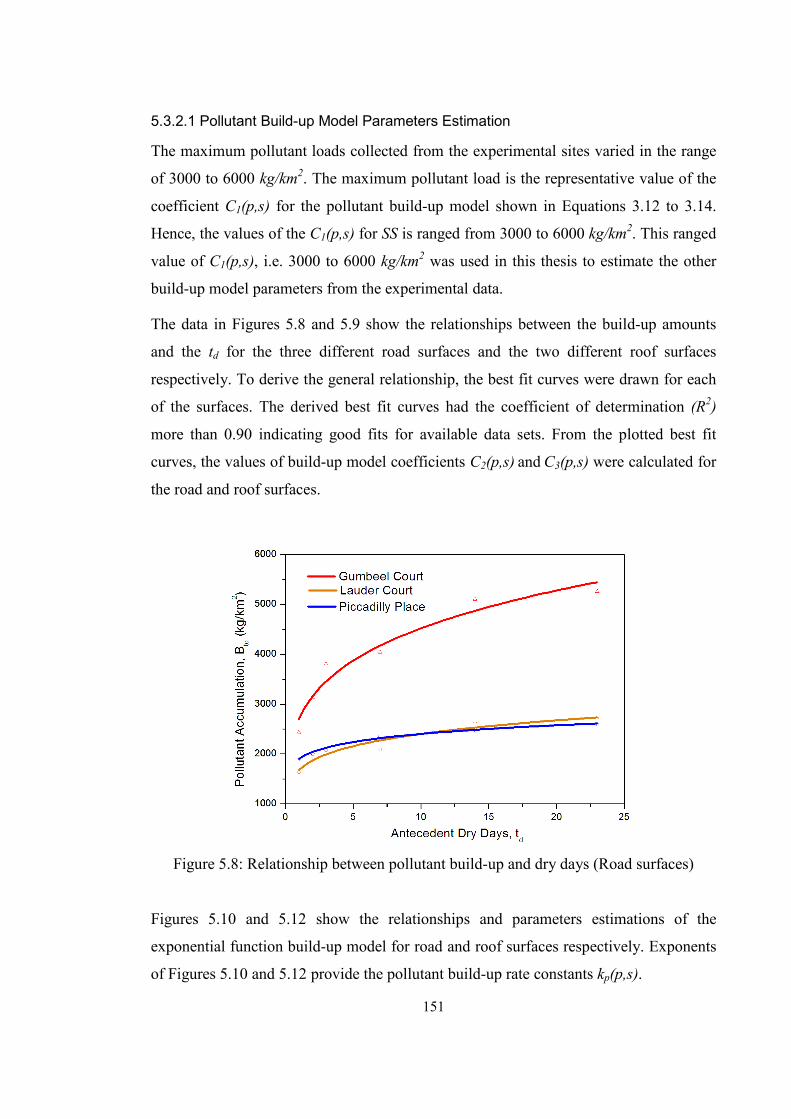
151

5.3.2.1 Pollutant Build-up Model Parameters Estimation

The maximum pollutant loads collected from the experimental sites varied in the range

of 3000 to 6000 kg/km2. The maximum pollutant load is the representative value of the

coefficient C1(p,s) for the pollutant build-up model shown in Equations 3.12 to 3.14.

Hence, the values of the C1(p,s) for SS is ranged from 3000 to 6000 kg/km2. This ranged

value of C1(p,s), i.e. 3000 to 6000 kg/km2 was used in this thesis to estimate the other

build-up model parameters from the experimental data.

The data in Figures 5.8 and 5.9 show the relationships between the build-up amounts

and the td for the three different road surfaces and the two different roof surfaces

respectively. To derive the general relationship, the best fit curves were drawn for each

of the surfaces. The derived best fit curves had the coefficient of determination (R2)

more than 0.90 indicating good fits for available data sets. From the plotted best fit

curves, the values of build-up model coefficients C2(p,s) and C3(p,s) were calculated for

the road and roof surfaces.

Figure 5.8: Relationship between pollutant build-up and dry days (Road surfaces)

Figures 5.10 and 5.12 show the relationships and parameters estimations of the

exponential function build-up model for road and roof surfaces respectively. Exponents

of Figures 5.10 and 5.12 provide the pollutant build-up rate constants kp(p,s).

152

Figure 5.9: Relationship between pollutant build-up and dry days (Roof surfaces)

Figure 5.10: Exponential function build-up parameters estimation (Road surfaces)

Figures 5.11 and 5.13 show the parameters estimation of the saturation function build-

up model for the road and roof surfaces respectively. The slopes of the lines in Figures

5.11 and 5.13 passing through the origin represent values of the half saturation constant

tp(p,s). The estimated values of the road and roof surfaces build-up parameters are

shown in Table 5.7.

153

Figure 5.11: Saturation function build-up parameters estimation (Road surfaces)

Figure 5.12: Exponential function build-up parameters estimation (Roof surfaces)

From Figures 5.8 to 5.13, it is clear that the build-up model parameters of Gumbeel

Court road surface and Corrugated Steel roof surface catchments are higher than the

other catchments. Therefore, it can be concluded that water quality parameters vary

from catchment to catchment, and hence the generic outcomes from one model should

be used cautiously.

154

Figure 5.13: Saturation function build-up parameters estimation (Roof surfaces)

Table 5.7: The estimated values of SS build-up parameters

Catchment Catchment

Characteristics

C1(p,s)

(kg/km2)

C2(p,s)

( ⋅2kmkg)3Cday −

C3(p,s) kp(p,s)

(1/day)

tp(p,s)

(days)

Gumbeel

Court

Townhouse region

with high

population density

5300 2623.8 0.238 0.222 1.244

Lauder

Court

Single detached

housing

2750 1678.5 0.155 0.210 0.784

Piccadilly

Place

Region with low

population density

2600 1900.7 0.102 0.382 0.418

Concrete

Tile

Industrial and

commercial areas

850 424.22 0.208 0.188 1.208

Corrugated

Steel

Industrial and

commercial areas

1200 401.33 0.349 0.122 0.434

155

5.3.2.2 Wash-off Model Parameters

Similar to the pollutant build-up model parameters, the estimation of the wash-off

model parameters was performed from the experimental study done by Egodawatta

(2007). Based on available data, the ratios between pollutant wash-off Wt(p,s) and

remaining build-up ( )dt

B were calculated for different rainfall intensities and durations.

For the estimation of power function wash-off model parameters, graphs between

( )dtt BspW , vs. qA,t are plotted for both road and roof surfaces. Figure 5.14 shows the

graph for the road surface of Piccadilly place and Figure 5.15 shows the graph for the

concrete tile roof surface. Coefficients and exponents of the best fit curves provide the

values of the wash-off coefficient E1(p,s) and exponent E2(p,s) respectively. Similar

relationships were observed for the other catchments and roof surfaces.

Figure 5.16 shows the graph of Wt(p,s) vs. Qt, for the estimation of the rating curve

wash-off model parameters for the Gumbeel Court road surface catchment. Similarly,

the estimation of the rating curve wash-off model parameters for roof surfaces was

performed. Figure 5.17 shows the graph of Wt(p,s) vs. Qt for the corrugated steel roof

surface. Like the power function wash-off model parameters estimation, coefficients

and exponents of the best fit equation provided the wash-off model parameters E3(p,s)

and E4(p,s) for the rating curve function.

Figure 5.14: Power function wash-off model parameters estimation (Road surfaces)

156

Figure 5.15: Power function wash-off model parameters estimation (Roof surfaces)

Figure 5.16: Rating curve wash-off model parameters estimation (Road surface)

For the estimation of the exponential wash-off model parameters, graphs between

( )spWB ttd,− vs. Itt were plotted for Lauder Court road surface and concrete tile roof

surface shown in Figures 5.18 and 5.19 respectively. Road and roof surfaces in other

catchments also followed the similar pattern. Exponents of Figures 5.18 and 5.19 are the

wash-off parameter E5(p,s) of the exponential wash-off model.

157

Figure 5.17: Rating curve wash-off model parameters estimation (Roof surface)

Figure 5.18: Exponential wash-off model parameters estimation (Road surface)

The summary of the estimated values of the wash-off model parameters for both the

road surface and roof surface catchments are shown in Table 5.8. Alike the build-up

model parameters, the wash-off model parameters from experimental data were

performed only for SS. Similar experimental studies should be performed to determine

the model parameters for other pollutants.

158

Figure 5.19: Exponential wash-off model parameters estimation

(Roof surface catchment)

Table 5.8: Estimated values of wash-off model parameters for SS

Catchments E1(p,s)

[ ] 2Ehrmm −

E2(p,s) E3(p,s)

[ ] 43. Esmkg −

E4(p,s) E5(p,s)

1/mm

Gumbeel

Court

0.0029 -

0.0135

0.608 -

0.986

3414.4 -

5260.4

0.472 -

0.580

0.011

Lauder

Court

0.0015 -

0.0059

0.945 -

1.270

1649.0 -

2927.8

0.344 -

0.744

0.028

Piccadilly

Place

0.0062 -

0.011

0.753 -

0.914

1864.6 -

2992.1

0.413 -

0.564

0.026

Concrete

Tile

0.051 -

0.202

0.363 -

0.603

585 - 805 0.556 -

0.797

0.388

Corrugated

Steel

0.112 -

0.213

0.333 -

0.414

2362 - 2685 0.993 -

1.000

0.134

159

5.3.3 Water Quality Model Parameters from Observed Field Data

With the available observed water quality data, the parameters for the pollutant

component of the catchment water quality model were determined by the calibration

procedure. Calibration of the build-up model and the wash-off model were performed

separately to estimate the required build-up and wash-off model parameters. Transferred

pollutants from catchment surfaces can be from either an impervious surface or a

pervious surface or both. Hence, the parameters for the catchment water quality model

were estimated for impervious and pervious surfaces separately. For each calibration

run, the measured and predicted water quality was matched to achieve required

pollutant transportation. This was done by adjusting the input parameters of the

developed model.

However, different researchers observed that the values of the build-up and wash-off

models parameters changed not only from catchment to catchment but also for rainfall

events. Berretta et al. (2007) noted that a single characteristic is not comprehensive in

describing the complexity of the model parameters affecting the both pollutant build-up

and wash-off processes. Therefore, the estimation of the model parameters should be

performed for a range of rainfall events. In this study, calibration was performed for

several continuous rainfall-runoff events, so that the accurate and reliable parameters

estimation could be achieved. Beven and Binley (1992); Volk et al. (2009) noted that

there is no possibility to expect that any one set of parameters will represent a true

parameter set. That’s why a range of parameters were estimated for the developed

model.

Calibration of the both sub-models (build-up model and wash-off model) was done

simultaneously until the total predicted pollutant loadings matched with the measured

field observation. However, water quality at the beginning of a rainfall event will be

dominated by the estimated build-up model parameters. It should be noted that for the

current calibration, the upper most sub-catchments were selected to get unaltered

pollutants transported only from the catchments, i.e. to avoid water quality samples

without pollutants degradation within the stream, and to avoid the tidal effects of the

stream.

160

5.3.3.1 Build-up Model Parameters

The build-up model was developed by considering the td as the predominant parameter.

The accuracy of pollutants prediction depends on the proper calculation of the td. The

initial value of the td was determined after analysing rainfall data. For the continuous

simulation, intermediate dry days were calculated by the model itself. Initially, the

build-up model parameters were selected based on information available in literature.

These parameters were progressively refined along with the pollutant wash-off model

parameters until an acceptable calibration was achieved for a range of rainfall events.

The build-up model parameters were estimated before the estimation of the wash-off

model parameters because the wash-off loads are directly proportional to pollutant

build-up loads (Baffaut and Delleur 1990). For the estimation of the parameters,

calibration of the model was performed for several rainfall events in each simulation.

Table 5.9: Estimated values of build-up model parameters of SS for SWCC

Parameters Values Unit

IMPV PEV

C1(p,s) 6000 12000 kg/km2

C2(p,s) 2500 4500 ( ) 3.2 Cdaykmkg −

C3(p,s) 0.40 0.40 -

kp(p,s) 0.35 0.35 1/day

tp(p,s) 1.50 2.00 days

Table 5.10: Estimated values of the build-up model parameters for TN

Parameters

HTCC SWCC

Unit Values Values

IMPV PEV IMPV PEV

C1(p,s) 300 400 500 800 kg/km2

C2(p,s) 150 200 200 350 ( ) 3.2 Cdaykmkg −

C3(p,s) 0.45 0.45 0.45 0.45 -

kp(p,s) 0.23 0.23 0.50 0.50 1/day

tp(p,s) 2.00 3.00 1.50 2.00 days

161

The summary of the estimated build-up model parameters of SS for SWCC is shown in

Table 5.9. The summarised values of the estimated build-up model parameters for

HTCC and SWCC are shown in Tables 5.10 and 5.11 for TN and TP respectively. The

detailed estimations of the build-up model parameters are shown in Appendix B.

Table 5.11: Estimated values of the build-up model parameters for TP

Parameters

HTCC SWCC

Unit Values Values

IMPV PEV IMPV PEV

C1(p,s) 150 200 250 400 kg/km2

C2(p,s) 50 70 90 140 ( ) 3.2 Cdaykmkg −

C3(p,s) 0.15 0.15 0.15 0.15 -

kp(p,s) 0.15 0.15 0.10 0.10 1/day

tp(p,s) 4.00 6.00 4.00 6.00 days

5.3.3.2 Wash-off Model Parameters

Similar to the pollutant build-up model parameters, the wash-off model parameters were

calculated for the two catchments based on the available build-up and the instantaneous

hydrological characteristics of the catchments surfaces.

Table 5.12: Estimated values of the SS wash-off model parameters for SWCC

Parameters Values Unit

IMPV PEV

E1(p,s) 0.030 0.050 – 0.055 [ ] 2Ehrmm −

E2(p,s) 0.21 0.21 -

E3(p,s) 0.160 – 0.180 0.300 – 0.330 [ ] 43. Esmkg −

E4(p,s) 0.30 0.30 -

E5(p,s) 0.00180 0.00340 1/mm

162

Table 5.13: Estimated values of the wash-off model parameters for TN

Parameters

HTCC SWCC

Unit Values Values

IMPV PEV IMPV PEV

E1(p,s) 0.0013 –

0.0017

0.0024 –

0.0032

0.0040 –

0.0050

0.0065 –

0.0080 [ ] 2Ehrmm −

E2(p,s) 0.75 –

0.80

0.75 –

0.80

0.65 –

0.80

0.65 –

0.80

-

E3(p,s) 0.00040 0.00065 –

0.0007

0.0012 0.0020 [ ] 43. Esmkg −

E4(p,s) 0.90 0.90 0.84 –

0.90

0.84 –

0.90

-

E5(p,s) 0.00018 –

0.00035

0.00040 –

0.00065

0.0017 –

0.0020

0.0028 –

0.0035

1/mm

Table 5.14: Estimated values of the wash-off model parameters for TP

Parameters

HTCC SWCC

Unit Values Values

IMPV PEV IMPV PEV

E1(p,s) 0.00012 –

0.0005

0.0007 –

0.00021

0.00030 –

0.00040

0.00050 –

0.00070 [ ] 2Ehrmm −

E2(p,s) 0.75 –

0.90

0.75 –

0.90

0.75 –

0.90

0.75 –

0.90

E3(p,s) 0.000020 -

0.000040

0.000035 -

0.000070

0.00010 –

0.00016

0.00015 –

0.00028 [ ] 43. Esmkg −

E4(p,s) 0.78 –

0.88

0.78 –

0.88

0.70 –

0.80

0.70 –

0.80

E5(p,s) 0.000001

– 0.00010

0.000001

– 0.00020

0.00013 –

0.00030

0.00015 –

0.00050

1/mm

163

For the estimation of the wash-off model parameters, calibration of the model was

performed for several rainfall events in each simulation. The summary of the estimated

wash-off model parameters of SS is shown in Table 5.12 for SWCC; while Tables 5.13

and 5.14 summarises the estimated wash-off model parameters of TN and TP

respectively for both HTCC and SWCC. The detailed calculations of the wash-off

model parameters are shown in Appendix C.

5.3.4 Calibration Results

The simulation of SS wash-off with the calibrated parameters for SWCC is shown in

Figure 5.20 for both the power function and the rating curve wash-off models. For the

both simulations, the power function build-up model was selected. Although shapes of

pollutographs were the same for the both wash-off models, the initial transportation was

less with the rating curve wash-off model. As obvious pollutant build-up was the same

in the both wash-off models simulation. The results indicate that the capability of the

rating curve wash-off model to simulate the FF phenomenon of SS was less for SWCC.

Also Deletic and Maksimovic (1998) found that FF occurs only in a limited number of

storm events.

Figure 5.20: Simulation of SS with the power function build-up (SWCC)

164

It was also observed in Figure 5.20 that during the middle period of the storm event,

there was less SS transportation with the power function wash-off model compared to

the rating curve wash-off model. This was due to the available SS on the catchment

surfaces. As FF washed-off most of the accumulated SS for the power function wash-off

model, available pollutants were depleted during the middle period of the storm. For

both wash-off models, the parameters were adjusted to fit the simulated results with the

observed water quality data.

With the same build-up model (power function build-up model), the simulation and

calibration results of TN wash-off for SWCC is shown in Figure 5.21 for both the power

function and the rating curve wash-off models. Similar to the SS simulation, the

capability of the rating curve wash-off model to simulate the FF phenomenon of TN was

less in compared to the power function wash-off model. However, there was also the

higher TN wash-off during the remaining period of the storm for the power function

wash-off model. This difference may be due to the selection of the wash-off model

parameters. More observed data is needed to establish the accurate wash-off model

parameters set.

Figure 5.21: Simulation of TN with the power function build-up

165

The simulation and calibration results of the TP wash-off with the power function build-

up model for SWCC is shown in Figure 5.22. Similar to the SS simulation, the shapes of

pollutographs were the same for both wash-off models for TP. However, the initial TP

wash-off results contradict with the both SS and TN simulations. The figure clearly

shows that the capability of the power function wash-off model to simulate FF for TP

was less compared to the rating curve wash-off model. There was also the higher TP

wash-off during the last period of the storm event for the power function wash-off

model. For this model, the amount of FF was not significant, leading to an increase

available TP to be washed-off during the reaming period of the storm. On the other

hand, for the rating curve wash-off model, available TP depleted with the significant FF

amount at the beginning of the storm leading to a lesser wash-off during the last period.

Figure 5.22: Simulation of TP with the power function build-up

The simulation results of the TN wash-off with the calibrated parameters for HTCC is

shown in Figure 5.23 for the power function and the rating curve wash-off models. For

both cases, the power function build-up model was used. Like SWCC, although the

shapes of the pollutographs were the same in both wash-off models, the initial wash-off

were less for the rating curve wash-off model. However, the pollutant build-up was the

same for both wash-off models. Therefore, the capability of the rating curve wash-off

166

model to simulate the FF phenomenon of TN was also less for HTCC. It can also be

observed from the figure that there was no wash-off at the end of the storm for the

rating curve wash-off model. This was due to more pollutant being washed off during

the middle period of the storm for the rating curve wash-off model leaving no available

TN to be washed off before the end of the storm.

Figure 5.23: Simulation of TN for the power function build-up model (HTCC)

Figure 5.24: Simulation of TN for the exponential build-up model (HTCC)

167

Figure 5.24 shows the simulation results of TP for the two wash-off models (power

function and rating curve) with the exponential build-up model for HTCC. From the

figure, it is clear that there was less TP wash-off during the initial period of the storm

event for the rating curve wash-off model. The simulated results of TP wash-off with

the power function build-up model for HTCC is shown in Figure 5.25 for the power

function and rating curve wash-off models. Like the TN wash-off, the shapes of the

pollutographs were the same for the both wash-off models for TP. However, the initial

TP wash-off was the same for the both wash-off models which contradict with the TN

results.

Figure 5.25: Simulation of TP for the power function build-up model (HTCC)

Figure 5.26 shows the simulation results of TP for the power function and rating curve

wash-off models with the exponential build-up model for HTCC. Similar to SWCC, the

power function wash-off was more suitable for simulating the FF phenomenon for TP.

Also there was the higher TP wash-off for the power function wash-off model at the end

of the wash-off simulation period. As there was no FF for this case, there were more

available pollutants to be washed-off with a higher rate of surface water. Due to less

available TP for the rating curve wash-off model at the end, the wash-off was less. This

indicates the dependency of TP wash-off to the available TP on the catchment surfaces.

168

The overall agreement of the simulated results with the observed data for the selected

water quality parameters appear to be good. The general simulation results of the model

with the calibrated parameters also looked reasonable, although these simulation

scenarios depend on the values of coefficients/parameters used in the model equations.

However, the results are promising and may be used for other catchments with similar

conditions.

Figure 5.26: Simulation of TP for the exponential build-up model (HTCC)

Although the observed data lay very close to the simulated results, there were small

variations between the observed data and the simulated results. The reason for this small

variation may be the build-up/wash-off parameters being not representative for the

study catchments. In addition, these differences among sub-models are due to the

different level of complexity of systems being modelled and are likely due to data

uncertainty. Indeed, it is reasonable to suppose that the quality the data measured

behave with a higher uncertainty level that, of course, influences modelling processes.

Due to the limitation of data, the comparisons with only one observation were shown.

Therefore, care should be taken when using these findings. More observed data is

needed to check the better capability of the model.

169

5.4 Stream Water Quality Model Parameters Similar to the catchment water quality model, the developed stream water quality model

needs to be correctly calibrated and verified for a particular stream reach before its use

in the reliable prediction of water quality parameters. Based on the available observed

field data, the parameters of the stream water quality model were determined for

Saltwater Creek which is located at Gold Coast, Australia. The stream water quality

model is comprised of two sub-models, i.e. streamflow and stream pollutants processes.

Therefore, it was necessary to estimate the parameters for both streamflow and

pollutants processes.

In this research project, the estimation of the flow parameters and the pollutant

parameters were performed separately. Usually, the output of the quantity model is used

as the input of the quality model. Hence, the quantity model parameters were calibrated

prior to its use in the quality model. Calibration of the model was done in two steps. In

the first step, the quantity parameters were calibrated and evaluated by comparing the

model output with widely used models. In the second step, the calibrated values of the

quantity model parameters were set to determine the quality model parameters. During

the calibration procedure, the parameters were varied individually and by means of

combinations until a good agreement between the modelling output and measured data

were achieved.

5.4.1 Streamflow Parameters Estimation

Estimation of the streamflow parameters required calibration of the Muskingum-Cunge

parameters. The stability of the Muskingum-Cunge method is accomplished, if the

routing time interval ∆tR falls between the limits 2KstorXP and 2Kstor (1-XP) (CRC for

Catchment Hydrology 2005). The theoretical value of Kstor is the time required for an

elemental (kinematic) wave to transverse through a particular stream reach. It is taken as

approximate the time interval between the inflow and the outflow peaks, if data are

available. If not, the wave velocity can be estimated for various channel shapes as a

function of average velocity ( )u for any representative flow rate. The average velocity

for steady uniform flow can be estimated by either the Manning’s or Chezy equation.

Table 5.15 shows velocities for various channel shapes.

170

Table 5.15: Kinematic wave velocities (Veissman and Lewis 2003)

Channel Shape Manning equation Chézy equation

Wide rectangular ( )u35 ( )u23

Triangular ( )u34 ( )u45

Wide Parabola ( )u911 ( )u67

For some stream reaches, it is possible that the selection of the reasonable values of

Kstor, XP and ∆tR will cause one or two routing coefficients to be negative. Such negative

coefficients could create negative outflows which is physically unreasonable and causes

the routing procedure to be mathematically incompatible. Therefore, the challenge in

the application of the Muskingum-Cunge method is the determination of the reasonable

values of the parameters Kstor and XP (Seybert 2006). In order to use the method with

confidence, Kstor and XP should be determined through the analysis of stream gauge

information where both upstream and downstream hydrographs are known. However, in

practice, these types of data are rarely available. Therefore, the practical application of

the Muskingum-Cunge method requires adoption of some guiding rules of thumb that

have some logical meaning. MUSIC deems that the values of Kstor and XP remain

constant within a stream reach throughout the simulation.

5.4.1.1 Stream Reach Storage Parameter

In Equations 3.27 to 3.29, Kstor is referred as the channel reach storage parameter of

storage delay time for a particular stream reach. The application of these equations has

shown that Kstor is usually close to the wave travel time. It has the dimension of time

and can be shown as the time between the centres of mass of the inflow hydrograph and

the outflow hydrograph. Furthermore, it is approximately equal to the travel time of a

flood wave through channel reach and can be approximated by dividing the channel

reach length by the celerity of the flood wave (CRC for Catchment Hydrology 2005). In

some cases, this time is almost constant regardless of the size of flood so that the

storage is a linear function of weighted average discharge, and the storage is said to be

linear. However, in general, travel time varies with the size of the flood wave and in

such cases the storage function is non-linear.

171

It should be noted that in the developed streamflow model, there are two different

options for the calculation of Kstor, i.e. fixed and variable with the depth of flow. The

fixed value of Kstor is given by the users as an input parameter; while the variable Kstor is

determined by the model automatically from the reach length and the depth of flow. The

final calibrated value of Kstor is 0.30 for Saltwater Creek when it was assumed to be

fixed.

5.4.1.2 Prism Parameter

In the Muskingum-Cunge method, the prism parameter XP is the weighting factor that

proportions the relative effects of the upstream section and the downstream section on

the ability of a channel to store water. This parameter reflects the ability to affects

channel storage capacity. Since the Muskingum-Cunge method assumes that the

upstream section and the downstream section are similar in the geometry and hydraulic

characteristics, the reasonable value of XP ranged from 0.00 to 0.50 (Seybert 2006;

Linsley et al. 1992). For the natural channel, it is generally ranged between 0.10 and

0.30 (Linsley et al. 1992); while the average value of XP is 0.20 (Seybert 2006;

Veissman and Lewis 2003).

However, it is often difficult to avoid the negative values of the outflow hydrograph,

especially when the value of XP is outside the range of 0.10 to 0.49 (CRC for Catchment

Hydrology 2005). Therefore, the developed model limits the value of XP between 0.10

and 0.49. Since data for Saltwater Creek was available, the parameters of the stream

water quality model were estimated for this creek. The final estimated value of XP for

Saltwater Creek was 0.30.

5.4.1.3 Other Parameters

For Saltwater Creek, stage-discharge parameters (‘a’ and ‘b’) were estimated by using

the HEC RAS model which is a widely used hydraulic model throughout the world. The

compensation coefficients (CFc and CFe) were determined from the relationship

between the hydraulic radius and the depth of flow as shown in Figure 5.27. The final

adopted values of the stage-discharge parameters and compensation factors are shown

in Table 5.16.

172

Figure 5.27: Estimation of compensation factor for Saltwater Creek

Table 5.16: Values of the streamflow model parameters

Parameters Symbol Values Unit

Stage-discharge parameter a 0.2812 -

Stage-discharge parameter b 0.4009 -

Coefficient for compensation factor CFc 0.542 -

Exponent for compensation factor CFe 0.980 -

5.4.1.4 Hydraulic Modelling Results

With the estimated parameters of the hydraulic model, the simulation results were

compared with the MUSIC model. As no runoff measurement was conducted for

Saltwater creek during the calibration period, the simulation results of the developed

model were compared with MUSIC, which is widely used model in Australia. In

addition, both the developed model and MUSIC used the Muskingum-Cunge method

for stream routing; the modelling results were compared with MUSIC. Figure 5.28

shows the plotted results of the comparison. It can be seen from the figure that there was

agreement between the simulated results and the MUSIC results, which indicates the

suitability of the hydraulic model in streamflow prediction.

173

For the statistical comparison with MUSIC, two error statistics PBIAS (percent bias)

and NSE (Nash Sutcliffe efficiency) were also computed. Since there was no observed

data, these comparisons were made with the MUSIC results. The computed value of

PBIAS was -0.073; whereas the optimal value is zero. On the other hand, NSE value for

the model was 0.963; whereas the optimal value is 1.0. Hence, the model can be used

for the runoff estimation of a particular stream reach.

Figure 5.28: Comparison of streamflow

5.4.2 Water Quality Parameters Estimation

The water quality component of the stream water quality model consists of SS, nutrients

and BOD processes. Therefore, it was necessary to estimate the parameters of the

relevant processes before its application to the practical problems. For this component

of the stream water quality model, it was required to estimate the parameters of SS

processes, the rate coefficients of both nutrients (TN and TP) and BOD. Based on the

estimated discharges of the hydraulic model and available observed field data of water

borne pollutants, the parameters of SS, BOD and nutrients models were determined. The

model was fitted with the observed field data collected from Saltwater Creek, Gold

Coast, Australia.

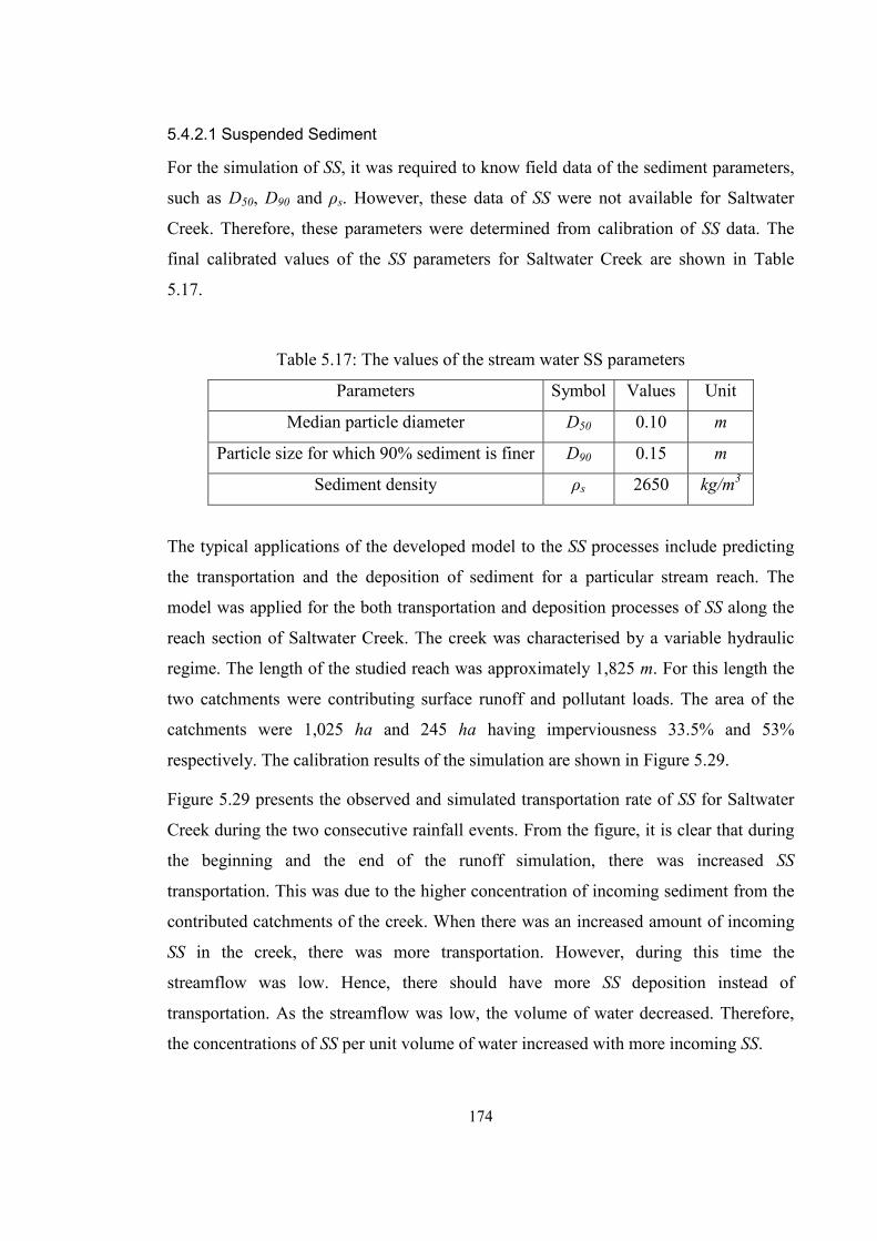
174

5.4.2.1 Suspended Sediment

For the simulation of SS, it was required to know field data of the sediment parameters,

such as D50, D90 and ρs. However, these data of SS were not available for Saltwater

Creek. Therefore, these parameters were determined from calibration of SS data. The

final calibrated values of the SS parameters for Saltwater Creek are shown in Table

5.17.

Table 5.17: The values of the stream water SS parameters


Median particle diameter D50 0.10 m

Particle size for which 90% sediment is finer D90 0.15 m

Sediment density ρs 2650 kg/m3

The typical applications of the developed model to the SS processes include predicting

the transportation and the deposition of sediment for a particular stream reach. The

model was applied for the both transportation and deposition processes of SS along the

reach section of Saltwater Creek. The creek was characterised by a variable hydraulic

regime. The length of the studied reach was approximately 1,825 m. For this length the

two catchments were contributing surface runoff and pollutant loads. The area of the

catchments were 1,025 ha and 245 ha having imperviousness 33.5% and 53%

respectively. The calibration results of the simulation are shown in Figure 5.29.

Figure 5.29 presents the observed and simulated transportation rate of SS for Saltwater

Creek during the two consecutive rainfall events. From the figure, it is clear that during

the beginning and the end of the runoff simulation, there was increased SS

transportation. This was due to the higher concentration of incoming sediment from the

contributed catchments of the creek. When there was an increased amount of incoming

SS in the creek, there was more transportation. However, during this time the

streamflow was low. Hence, there should have more SS deposition instead of

transportation. As the streamflow was low, the volume of water decreased. Therefore,

the concentrations of SS per unit volume of water increased with more incoming SS.

175

Figure 5.29: Simulation of SS transport for the Saltwater Creek

On the other hand, there should be more SS deposition with the increased incoming

sediment concentration. However, when the transport capacity of the streamflow

increases the deposition rate decreases. For the creek, the transport capacity of the flow

was strong enough to carry all SS to the downstream at that time. Hence, the

transportable SS concentration was higher during the beginning and the end of the

simulation even with the higher incoming sediment. However, the observed

concentration is very much closer to the simulated results indicating the good

performance of the model simulations shown in Figure 5.29. Due to the limitation of

data only one observation point was shown. For an accurate morphological prediction,

more observed data is needed.

There was a slight deviation of the simulated results from the observed data. This small

deviation can be attributed mainly due to the higher complexity of phenomena involved

in the sedimentation of SS. A slight miscalculation of these phenomena may contribute

to the higher disagreement between the observed and simulated values. In the

simulation of the model, only the mean diameter of the suspended particles was used.

The influence of the presence of various grain size fractions in the creek may be

responsible for the deviation. In addition, for the simplicity of the model, re-suspension

of the bed materials was not considered.

176

5.4.2.2 Parameters for the Reactive Pollutants

Similar to the parameters of the SS model, the parameters of the nutrients models were

estimated for Saltwater Creek. The parameters of the model were estimated with only

those water quality data which were collected during rainfall events. The initial values

of these parameters were selected from available literature. However, most of the other

studies were done by considering fragmental components of the nutrients processes.

This study concentrated on estimating the rate parameters for total nutrients, instead of

fragmental determination. The values of rate coefficients were estimated by the

calibration procedure. Table 5.18 summarises the calibrated values of rate coefficients

of the reactive pollutants, i.e. BOD, TN and TP. The plotted results of the simulation are

shown in Figures 5.30 and 5.31 for TN and TP respectively. The simulation was

performed with the calibrated parameters and the predicted values were compared with

the observed field data.

Table 5.18: The estimated parameters of the reactive pollutants


Rate of oxidation of BOD kBOD 0.23 (1/day)

Rate of BOD loss due to settling ksBOD - (1/day)

Re-suspension rate of BOD ksusBOD - (1/day)

Half saturation constant for BOD Ks - (1/day)

Denitrification coefficient of TN kDEN 0.35 (1/day)

Release rate of TN from BOD kTN 0.75 (1/day)

Release rate of TN from sediment ksTN 0.65 (1/day)

Release rate of TP from BOD kTP 0.40 (1/day)

Release rate of TP from sediment ksTP 0.35 (1/day)

Adjustment factor for sediment TP release δTP 0.31 -

From Figures 5.30 and 5.31, it is clear that at the beginning and the end of the

simulation, there were more pollutant transportation through the creek. However, during

these times, the creek discharge was less. As a result, pollutants per unit discharge

increased; and hence the transported pollutant concentrations were higher.

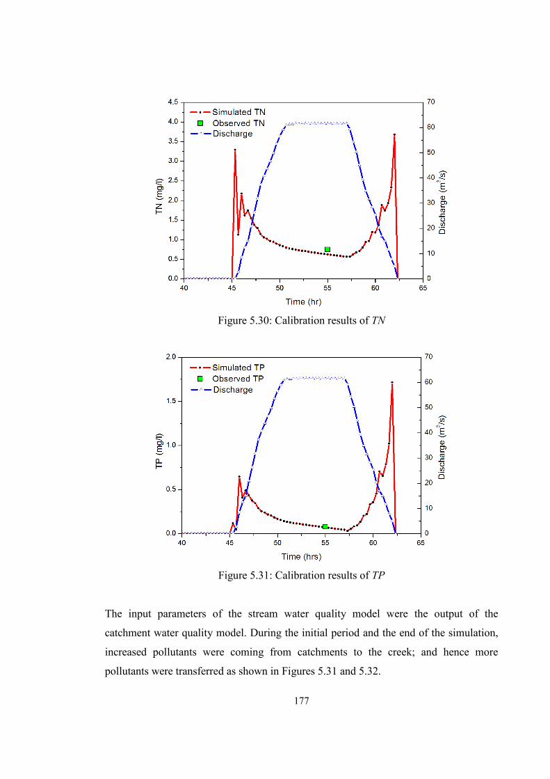
177

Figure 5.30: Calibration results of TN

Figure 5.31: Calibration results of TP

The input parameters of the stream water quality model were the output of the

catchment water quality model. During the initial period and the end of the simulation,

increased pollutants were coming from catchments to the creek; and hence more

pollutants were transferred as shown in Figures 5.31 and 5.32.

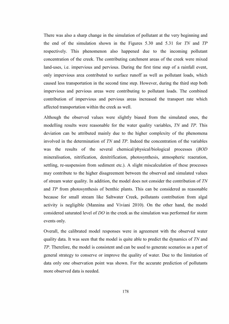
178

There was also a sharp change in the simulation of pollutant at the very beginning and

the end of the simulation shown in the Figures 5.30 and 5.31 for TN and TP

respectively. This phenomenon also happened due to the incoming pollutant

concentration of the creek. The contributing catchment areas of the creek were mixed

land-uses, i.e. impervious and pervious. During the first time step of a rainfall event,

only impervious area contributed to surface runoff as well as pollutant loads, which

caused less transportation in the second time step. However, during the third step both

impervious and pervious areas were contributing to pollutant loads. The combined

contribution of impervious and pervious areas increased the transport rate which

affected transportation within the creek as well.

Although the observed values were slightly biased from the simulated ones, the

modelling results were reasonable for the water quality variables, TN and TP. This

deviation can be attributed mainly due to the higher complexity of the phenomena

involved in the determination of TN and TP. Indeed the concentration of the variables

was the results of the several chemical/physical/biological processes (BOD

mineralisation, nitrification, denitrification, photosynthesis, atmospheric reaeration,

settling, re-suspension from sediment etc.). A slight miscalculation of these processes

may contribute to the higher disagreement between the observed and simulated values

of stream water quality. In addition, the model does not consider the contribution of TN

and TP from photosynthesis of benthic plants. This can be considered as reasonable

because for small stream like Saltwater Creek, pollutants contribution from algal

activity is negligible (Mannina and Viviani 2010). On the other hand, the model

considered saturated level of DO in the creek as the simulation was performed for storm

events only.

Overall, the calibrated model responses were in agreement with the observed water

quality data. It was seen that the model is quite able to predict the dynamics of TN and

TP. Therefore, the model is consistent and can be used to generate scenarios as a part of

general strategy to conserve or improve the quality of water. Due to the limitation of

data only one observation point was shown. For the accurate prediction of pollutants

more observed data is needed.

179

5.5 Conclusions It is widely accepted that effective and efficient pollution mitigation strategies of a

particular watershed area depend on the water quality modelling results. However, the

practical application of any mathematical model depends on the proper selection of the

appropriate model parameters. The detailed knowledge of the controlling model

parameters of any water quality model will help for the reliable prediction of water

borne pollutants.

The ideal method to determine the water quality model parameters is the adoption of the

calibration procedure using adequate and reliable hydrologic and water quality data. In

the absence of adequate data, models are calibrated by visual comparison with other

widely used models or from information of available literature. If regional equations

(correlating to the model parameters to the watershed basins and other details) are

available, they can be used to estimate the model parameters. However, to derive

regional equations, it is also necessary to determine the model parameters accurately

through the calibration procedure. Hence, for the application of the developed integrated

model, it is necessary to estimate the required model parameters.

This chapter of the thesis has presented the results of the research undertaken to

estimate the parameters of the developed integrated catchment-stream water quality

model. The aim was to estimate the regional parameters of the model. The model

parameters were estimated from the both experimental and measured field data. Since

the output of the catchment water quality model is used as the input of the stream water

quality model, the catchment water quality model parameters were determined before

the estimation of the stream water quality model parameters by the calibration

procedure. The calibrated model parameters revealed which of the different model

equations best represented the field data to catchment and stream.

Calibration of the model was intended to determine a range of parameter values for the

both water quantity and quality models. Calibration of the model was made by means of

an iterative process of trial and error by adjusting the parameters and comparing the

simulation results with the observed data. Calibration of the catchment water quality

model was demonstrated for two catchments (HTCC and SWCC), Gold Coast, eastern

Australia.

180

The runoff estimation from the hydrologic model was compared with the calculated

discharges from widely used Australian runoff models, i.e. the rational method, WBNM

and DRAINS. HTCC is predominantly pervious with only 2.41% imperviousness. So,

the pervious surface parameters can be considered as the dominating parameters of the

model for HTCC. On the other hand, SWCC is of mixed land-use with 33.5%

impervious. So, both impervious and pervious surfaces dominated the pollutant

accumulation and transportation for SWCC. Therefore, the values of the model

parameters were estimated for impervious and pervious surfaces separately.

Calibration of the stream water quality model was performed for Saltwater Creek. The

output of the catchment water quality model was used as the input of the stream water

quality model. The estimated discharges of the streamflow model were evaluated and

compared with the calculated streamflow of MUSIC and HEC RAS which are widely

used models in Australia. The initial values of the rate parameters of the reactive

pollutants were determined from available literature.

After estimating the model parameters from the observed data, it can be concluded that

the dynamics of the non-point source pollutants build-up and wash-off are still not well-

known. The water quality component of the model is much more complex having many

parameters/coefficients to be determined. The model parameters vary a lot depending on

geographical locations, land-uses and the percentage of imperviousness of catchment

surfaces. The values of coefficients and exponents are different for each of the water

quality parameters associated with the build-up and wash-off models. This is to be

expected because each pollutant has different accumulation and transformation

behaviour. The model parameters were treated as the spatially and temporally averaged

constants.

Comparing the observed field data with the simulated results using the calibrated

parameters, it was found that the results are satisfactory. The model provided excellent

representation of the field data demonstrating the simplicity yet effectiveness of the

proposed model. The estimated parameters can be used for the analysis of the long term

pollutants behaviour and the impact of the land-use changes. They parameters are

expected to be useful for the future use of the model and to the development of BMPs in

this region.

181

The outcomes of the study suggest that the model is a possible tool, which will aid in

the development of management strategies for complex watershed areas like HTCC and

SWCC. The calibrated model responses are in agreement with the observed water

quality data. Therefore, the model is consistent and can be used to generate scenarios as

a part of the general strategies to conserve or improve the quality of water. The

calibrated model can be used to assess the effectiveness of management decisions.

It should be noted that calibration of the model parameters was performed with only a

limited number of observations. Therefore, care should be taken when using the

findings. Calibration of water quality models should be performed from real

measurements for a specific area for the continuous storm events. The ultimate

predictive capability of the model should be checked with the observed field data.

183

Chapter 6 Sensitivity of the Model Parameters

6.1 Introduction Sensitivity analysis is a formalised procedure to identify the changes in model responses

due to the changes in the various model parameters (Snowling and Kramer 2001). This

analysis forms an important part of the model validation process where model

development and data gathering activities are focused (Newham 2002). The sensitivity

of the model parameters illuminates information on the following types of questions

(Beres and Hawkins 2001):

Which of the model parameters exert a significant influence on the modelling

output?

Which parameters are inconsequential?

Do increments of any parameter produce unexpectedly large alterations in the

results?

Without answering these questions, proper understanding of any mathematical model

responses remains incomplete. Thus, sensitivity analysis is a significant aspect of every

modeller’s job.

The general purpose of sensitivity analysis is to determine which input parameters apply

the most influence on the model results (Dayaratne 2000). This analysis also helps to

acquire the detailed knowledge of the controlling model parameters of any particular

model. Sensitivity analysis increases the modeller’s understanding about the techniques

considered in the model development. Moreover, through sensitivity analysis, we can

learn how to select model complexity and how to improve the quality of information

derived from models for planning processes (Laenen and Dunnette 1997). In addition,

sensitivity analysis is used to give insights into interactions between the different

components of a mathematical model (Newham 2002). Therefore, Beres and Hawkins

(2001) noted that recommendations based upon a mathematical model without an

explicit sensitivity analysis lack a basic foundation.

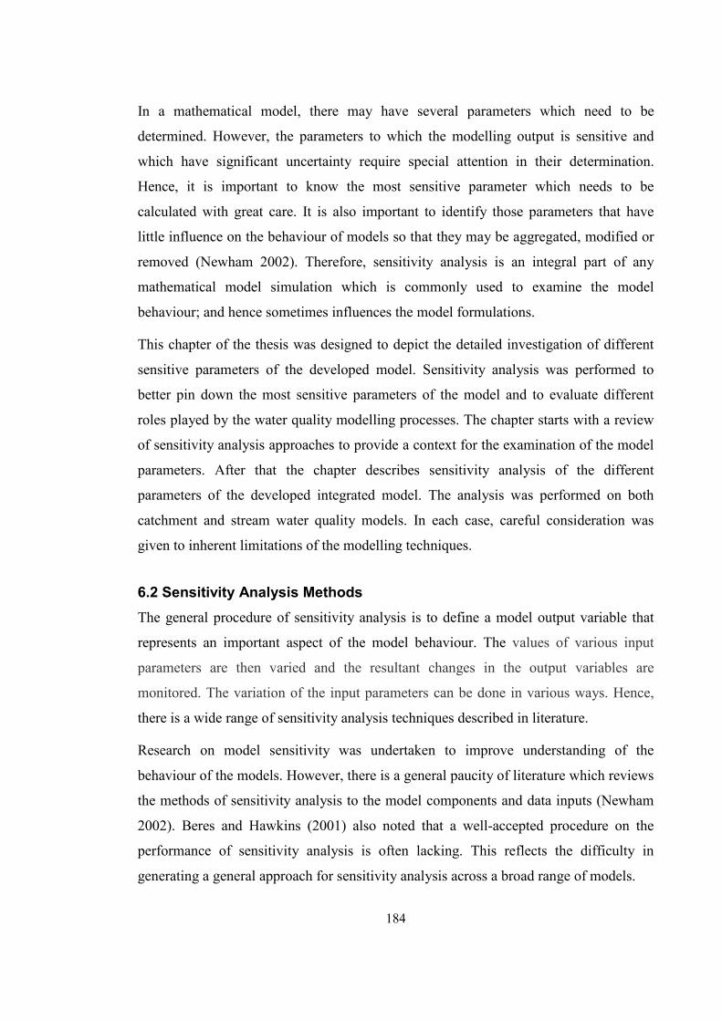
184

In a mathematical model, there may have several parameters which need to be

determined. However, the parameters to which the modelling output is sensitive and

which have significant uncertainty require special attention in their determination.

Hence, it is important to know the most sensitive parameter which needs to be

calculated with great care. It is also important to identify those parameters that have

little influence on the behaviour of models so that they may be aggregated, modified or

removed (Newham 2002). Therefore, sensitivity analysis is an integral part of any

mathematical model simulation which is commonly used to examine the model

behaviour; and hence sometimes influences the model formulations.

This chapter of the thesis was designed to depict the detailed investigation of different

sensitive parameters of the developed model. Sensitivity analysis was performed to

better pin down the most sensitive parameters of the model and to evaluate different

roles played by the water quality modelling processes. The chapter starts with a review

of sensitivity analysis approaches to provide a context for the examination of the model

parameters. After that the chapter describes sensitivity analysis of the different

parameters of the developed integrated model. The analysis was performed on both

catchment and stream water quality models. In each case, careful consideration was

given to inherent limitations of the modelling techniques.

6.2 Sensitivity Analysis Methods The general procedure of sensitivity analysis is to define a model output variable that

represents an important aspect of the model behaviour. The values of various input

parameters are then varied and the resultant changes in the output variables are

monitored. The variation of the input parameters can be done in various ways. Hence,

there is a wide range of sensitivity analysis techniques described in literature.

Research on model sensitivity was undertaken to improve understanding of the

behaviour of the models. However, there is a general paucity of literature which reviews

the methods of sensitivity analysis to the model components and data inputs (Newham

2002). Beres and Hawkins (2001) also noted that a well-accepted procedure on the

performance of sensitivity analysis is often lacking. This reflects the difficulty in

generating a general approach for sensitivity analysis across a broad range of models.

185

Campolongo et al. (2000) identified the three main settings of sensitivity analysis of a

mathematical model:

Factor screening: to identify the most influential factor in a system with many

factors

Local sensitivity analysis: to identify the local impact of the model parameters

and involves the use of partial derivatives

Global sensitivity: to identify the output uncertainty to the uncertainty in the

input parameters

The classification provides a useful means of structuring the current review of

sensitivity analysis. This information can be used to simplify the structure and

parameterisation of any mathematical model and its improvement for future application

to specific problems (Newham 2002).

Sensitivity analysis of the developed model was performed to a variety of model input

parameters, including the state variables, the environmental variables and the initial

conditions. The analysis of the model parameters was accomplished to assess the

importance of the various model parameters by showing how the simulation can be

changed with the changed input parameters. The factor screening sensitivity measure

was used for this research thesis. The screening method was chosen because it is useful

in dealing with models containing a large number of parameters (Newham 2002), and

the developed model contains a large number of parameters. In many respects, this

method is similar to the local sensitivity analysis technique. This procedure holds ‘‘all

other things are equal’’; while each parameter is altered to determine its effect in

isolation from the possible effects of other values (Beres and Hawkins 2001).

6.3 Sensitivity of the Catchment Water Quality Model Sensitivity analysis of the catchment water quality model was performed for the

investigation of two main phenomena. Firstly, the logical sensitivity of the model was

performed to investigate the capability of the continuous simulation and pollutant

availability on catchment surfaces. Secondly, the influences of the input model

parameters to the output were investigated to demonstrate the most influential

parameter.

186

6.3.1 Sensitivity to Model Capability

As a first step to demonstrate the usefulness and capability of the continuous simulation

of surface runoff and water quality parameters, the model was used to simulate runoff

and SS loads from a hypothetical catchment using the assumed values of the different

model parameters. The purpose was to assess whether the model was capable of

generating logical trends that are consistent with the expected runoff and pollutant

wash-off behaviour. The model was applied for the simulation of two different rainfall-

runoff and pollutant loads scenarios.

In the first simulation, two rainfall events were assumed to be 29 hours apart with

similar intensities, as shown in Figure 6.1. The chosen catchment had an area of 25 km2

and runoff slope of 1 m/km. The rainfall loss parameters were assumed to be in

accordance with IEAust (2001), with IL = 15 mm. The values of CL were assumed to

follow the exponentially decreasing loss model. Coefficients of the CL model were

assumed to be ACL = 1.5 and BCL = 3.0 so that the values of CL recline within the

recommended values suggested by ARR. For the calculation of the pollutant

accumulation on the catchment surfaces, the power function build-up equation was

used. The parameters of the power function build-up model for impervious surface

were: C1(p,s) = 6000 kg/km2, C2(p,s) = 2600 kg/km2, C3(p,s) = 0.16; and for pervious

surface were: C1(p,s) = 3000 kg/km2, C2(p,s) = 800 kg/km2, C3(p,s) = 0.16. For the

calculation of the transported pollutants, the power function wash-off model was used.

The values of the parameters used for the wash-off model were: E1(p,s) = 0.10, E2(p,s) =

0.15 for impervious surface area; and E1(p,s) = 0.07, E2(p,s) = 0.05 for pervious surface

area.

The plotted data in Figure 6.1 shows the rainfall and SS simulation results. The

simulation results of the model show that SS wash-off for the second rainfall event was

a little bit lower than the SS wash-off for the first event. Although the same rainfall

intensities were used for the both rainfall events, the SS wash-off for the first rainfall

event was the higher than that for the second rainfall event. This was because following

SS washed-out during the first event, the intermediate dry period was not long enough to

build-up significant additional SS to produce a higher wash-off during the second

rainfall event. In addition, there was no SS wash-off between the two rainfall events.

187

This phenomenon happened, because at that time there was no rainfall to produce

surface runoff which could transport pollutant loads from the catchment surfaces.

Similar wash-off patterns were observed for water quality parameters of TN and TP.

Figure 6.1: Simulation of rainfall and SS wash-off for isolated rainfall events

In the second simulation, the performance of the model in simulating a significant

continuous rainfall event of 32 hrs duration was tested. The values of the runoff and

pollutant model parameters, and catchment characteristics were the same as the first

simulation except the rainfall event. For a continuous rainfall event, rainfall loss

declines with time and surface runoff lasts for an extended period of time. However, the

pollutant wash-off is limited by the amount of available pollutants on a catchment

surface which is mostly removed during FF. The data in Figure 6.2 shows the

simulation of catchment runoff and SS simulation for the long continuous rainfall event.

The model simulation revealed the obvious FF phenomenon with significant SS wash-

off at the early stage of the storm. As rainfall continued, the pollutant wash-off

decreased with the time to negligible values. The data in Figure 6.2 also indicates that at

one stage of the decreasing trend, there was a sudden increase in wash-off generating a

localised SS peak, which can be attributed to the time difference between the arrival of

SS from impervious and pervious areas of the catchment.

188

Figure 6.2: Surface runoff and SS wash-off for a continuous rainfall event

Surface runoff from impervious area started earlier than from pervious surface. The

contribution of pervious surface SS starts upon the arrival of runoff from pervious

surface. Since both impervious surface and pervious surface started to wash-off

together, there was an increased SS wash-off as shown in Figure 6.2.

The above simulations demonstrated that the developed model is capable of generating

logical runoff and SS wash-off trends that are consistent with the expected behaviour.

However, the usefulness of the model required further testing using real data.

6.3.2 Parameters Sensitivity

To investigate the changes in the model output with the changes in the input parameters,

sensitivity analysis of the calibrated model parameters was performed. The calculated

model parameters were varied one at a time around standard (control) values and the

magnitude of residuals was compared in order to evaluate the parameters to which the

model is significantly sensitive. The purpose was to identify the most important

parameter from amongst a large number that may affect model responses. The analysis

was performed around the optimal calibrated parameters in order to assess the impact of

selecting the inaccurate values of the model parameters.

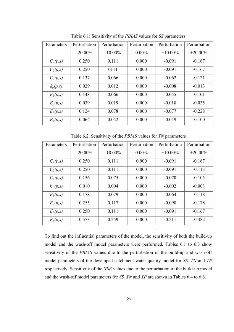
189

Table 6.1: Sensitivity of the PBIAS values for SS parameters

Parameters Perturbation

-20.00%

Perturbation

-10.00%

Perturbation

0.00%

Perturbation

+10.00%

Perturbation

+20.00%

C1(p,s) 0.250 0.111 0.000 -0.091 -0.167

C2(p,s) 0.250 0111 0.000 -0.091 -0.167

C3(p,s) 0.137 0.066 0.000 -0.062 -0.121

kp(p,s) 0.029 0.012 0.000 -0.008 -0.013

E1(p,s) 0.148 0.066 0.000 -0.055 -0.101

E2(p,s) 0.039 0.019 0.000 -0.018 -0.035

E3(p,s) 0.124 0.078 0.000 -0.077 -0.228

E4(p,s) 0.064 0.042 0.000 -0.049 -0.100

Table 6.2: Sensitivity of the PBIAS values for TN parameters


-20.00%

Perturbation

-10.00%

Perturbation

0.00%

Perturbation

+10.00%

Perturbation

+20.00%

C1(p,s) 0.250 0.111 0.000 -0.091 -0.167

C2(p,s) 0.250 0.111 0.000 -0.091 -0.113

C3(p,s) 0.156 0.075 0.000 -0.070 -0.105

k p(p,s) 0.010 0.004 0.000 -0.002 -0.003

E1(p,s) 0.178 0.079 0.000 -0.064 -0.118

E2(p,s) 0.255 0.117 0.000 -0.098 -0.178

E3(p,s) 0.250 0.111 0.000 -0.091 -0.167

E4(p,s) 0.573 0.259 0.000 -0.211 -0.382

To find out the influential parameters of the model, the sensitivity of both the build-up

model and the wash-off model parameters were performed. Tables 6.1 to 6.3 show

sensitivity of the PBIAS values due to the perturbation of the build-up and wash-off

model parameters of the developed catchment water quality model for SS, TN and TP

respectively. Sensitivity of the NSE values due to the perturbation of the build-up model

and the wash-off model parameters for SS, TN and TP are shown in Tables 6.4 to 6.6.

190

Table 6.3: Sensitivity of the PBIAS values for TP parameters


-20.00%

Perturbation

-10.00%

Perturbation

0.00%

Perturbation

+10.00%

Perturbation

+20.00%

C1(p,s) 0.249 0.111 0.000 -0.091 -0.167

C2(p,s) 0.250 0.112 0.000 -0.089 -0.167

C3(p,s) 0.049 0.025 0.000 -0.023 -0.047

k p(p,s) 0.144 0.063 0.000 -0.051 -0.093

E1(p,s) 0.239 0.106 0.000 -0.088 -0.161

E2(p,s) 0.451 0.205 0.000 -0.171 -0.313

E3(p,s) 0.248 0.082 0.000 -0.110 -0.166

E4(p,s) 0.425 0.197 0.000 -0.170 -0.314

Table 6.4: Sensitivity of the NSE values for SS parameters


-20.00%

Perturbation

-10.00%

Perturbation

0.00%

Perturbation

+10.00%

Perturbation

+20.00%

C1(p,s) 0.931 0.986 1.000 0.991 0.969

C2(p,s) 0.931 0.986 1.000 0.991 0.969

C3(p,s) 0.979 0.995 1.000 0.996 0.984

k p(p,s) 0.999 1.000 1.000 1.000 1.000

E1(p,s) 0.942 0.988 1.000 0.992 0.972

E2(p,s) 0.998 0.999 1.000 0.999 0.998

E3(p,s) 0.928 0.984 1.000 0.990 0.843

E4(p,s) 0.986 0.996 1.000 0.997 0.991

From Tables 6.1 to 6.6, it is clear that the maximum build-up rate C1(p,s) and the build-

up rate coefficient C2(p,s) were the sensitive parameters of the build-up model. A small

change in the values of the parameters C1(p,s) and C2(p,s), caused the large changes in

the statistical parameters PBIAS and NSE as can be seen in Tables 6.1 to 6.6 compared

with the build-up exponent C3(p,s) and the accumulation rate coefficient kp(p,s).

Therefore, these parameters C1(p,s) and C2(p,s) of the build-up model should be

estimated with great care. However, in between C3(p,s) and kp(p,s), the parameter kp(p,s)

was the least sensitive parameter.

191

Table 6.5: Sensitivity of the NSE values for TN parameters


-20.00%

Perturbation

-10.00%

Perturbation

0.00%

Perturbation

+10.00%

Perturbation

+20.00%

C1(p,s) 0.923 0.985 1.000 0.990 0.966

C2(p,s) 0.923 0.985 1.000 0.990 0.984

C3(p,s) 0.970 0.993 1.000 0.994 0.986

k p(p,s) 1.000 1.000 1.000 1.000 1.000

E1(p,s) 0.960 0.992 1.000 0.994 0.980

E2(p,s) 0.944 0.987 1.000 0.999 0.962

E3(p,s) 0.916 0.983 1.000 0.989 0.963

E4(p,s) 0.634 0.917 1.000 0.938 0.791

Table 6.6: Sensitivity of NSE values for TP parameters


-20.00%

Perturbation

-10.00%

Perturbation

0.00%

Perturbation

+10.00%

Perturbation

+20.00%

C1(p,s) 0.924 0.985 1.000 0.990 0.966

C2(p,s) 0.924 0.985 1.000 0.990 0.966

C3(p,s) 0.997 0.999 1.000 0.999 0.997

k p(p,s) 0.975 0.995 1.000 0.997 0.990

E1(p,s) 0.932 0.986 1.000 0.991 0.969

E2(p,s) 0.777 0.953 1.000 0.966 0.886

E3(p,s) 0.921 0.990 1.000 0.985 0.964

E4(p,s) 0.840 0.961 1.000 0.965 0.872

The changes in parameters C3(p,s) and kp(p,s) did not produce a significant change in

the modelling output; and hence in the PBIAS and NSE values. The variations of the

plotted results of sensitivity analysis are shown in Figures 6.3 to 6.6 for the build-up

model parameters; and Figures 6.7 to 6.10 for the wash-off parameters for SS. The

sensitivity of the build-up parameters followed the same pattern. The analysis was

performed by changing each parameter; while keeping others constant and observing

the changes in the model output.

192

Similar to the build-up model parameters, Tables 6.1 to 6.3 show the changes in the

PBIAS values; and Tables 6.4 to 6.6 show the changes in the NSE values due to the

perturbation of the wash-off model parameters. The plotted variations of the percentage

output change in pollutant loads to the perturbation of the wash-off model parameters

are shown in Figures 6.3 to 6.6 for SS. The variations in the sensitivity of the wash-off

model parameters for the other pollutants (TN and TP) follow the same pattern.

Figure 6.3: Sensitivity of the build-up parameter C1(p,s) for SS


193


Figure 6.6: Sensitivity of the build-up parameter kp(p,s) for SS

From Tables 6.1 to 6.6 and Figures 6.7 to 6.10, it is clear that the pollutant wash-off

coefficient E1(p,s) was the most sensitive parameter for the power function wash-off

model. On the other hand, for the rating curve wash-off model, the coefficient of the

rating curve wash-off function E2(p,s) was the most sensitive parameter. The changes in

all other parameters did not produce a significant change in the simulation results.

194

For both the power function and the rating curve wash-off models, the output variations

were much larger during the peak flow. The large changes in the output variables imply

that the particular input variable is important in controlling the model behaviour.

Similar to SS, the results for TN and TP follow the same pattern of sensitivity. It should

be noted that the output responses were non-linear across the examined parameters.

Figure 6.7: Sensitivity of the wash-off model parameter E1(p,s) for SS


195



6.4 Sensitivity of the Stream Water Quality Model Similar to the catchment water quality model, sensitivity analysis of the developed

stream water quality model was also performed to assess the most influential parameter.

For this analysis, a 1,825 m section of Saltwater Creek was chosen. Since the model was

comprised of two sub-models, i.e. streamflow and stream pollutants processes, the

sensitivity of the parameters were performed for the both sub-models.

196

6.4.1 Sensitivity of Streamflow Parameters

Sensitivity analysis of the developed streamflow model parameters was performed to

assess their effects on the simulation of stream water quantity. Since, the measured

streamflow data were not available; this assessment was accomplished with the

commercially available models, MUSIC and HEC RAS. The comparisons of the plotted

results are illustrated in Figures 5.11 to 5.13.

Figure 6.11: Sensitivity with other models with variable Kstor values

From Figure 6.11, it is clear that the simulated streamflow hydrograph was very much

closer to the hydrograph of MUSIC, which was much higher than the simulated results

of the HEC RAS model. This was reasonable because both the developed model and

MUSIC used the Muskingum-Cunge method for the prediction of downstream

discharges of the creek. The Muskingum-Cunge method was developed based on the

equation of continuity. On the other hand, the HEC RAS streamflow simulation was

calculated by solving the energy equation with an iterative procedure called the standard

step method. For the simulation of the HEC RAS model, the value of Manning’s

roughness coefficient was assumed to 0.03. Since the Muskingum-Cunge method does

not require the value of Manning’s ‘n’, it was not considered for the developed model

and for MUSIC.

197

The value of Kstor was determined to 15 minutes for MUSIC. For the developed model,

the value of Kstor was variable with the depth of flow. The value of the other routing

parameter XP was assumed to 0.15 both for MUSIC and for the developed model. A

large difference between the model simulation and the HEC RAS simulation was also

observed.

When the simulation of the developed model was performed with the fixed Kstor value,

the output response was very close to the calculated discharges of the HEC RAS model.

However, the simulation results deviated from the estimated flows of MUSIC as shown

in Figure 6.12. This slight deviation was due to the consideration of the fixed value of

Kstor. Therefore, we can conclude that there is a relationship between the Muskingum

parameter Kstor and the standard step method of energy equation. The future research

direction will be focused on the exploration of this relationship.

Figure 6.12: Sensitivity with other models with fixed Kstor value

The sensitivity of the Manning’s ‘n’ values of the HEC RAS model was also performed.

For this analysis, the value of XP was 0.15; and the value of Kstor was fixed to 15

minutes for the developed model. Figure 6.13 demonstrates the sensitivity of the HEC

RAS model with different Manning’s ‘n’ values and their comparison with the

developed model.

198

Figure 6.13: Sensitivity with the HEC RAS model different ‘n’ values

From Figure 6.13, it is clear that the lower ‘n’ values produced the higher peak

discharge and the higher ‘n’ values created the lower peak discharge in the HEC RAS

model. It is reasonable because the higher ‘n’ value means more friction and the

reduced peak. The figure also reveals that the model responses were very much closer to

the calculated discharges of HEC RAS with n = 0.030. This was also reasonable

because the usual value of Manning’s ‘n’ is 0.030 for a natural stream.

6.4.2 Sensitivity of SS Parameters

The predominant mode for the sediment transportation and deposition depends on the

size, shape and density of particles in respect to the velocity and turbulence field of

water bodies (Celik and Rodi 1989). To identify the influential parameters of SS, the

developed model was simulated under different scenarios. The individual simulation

runs for the transportation and deposition of SS were performed on the basis of

streamflow, the inflow sediment concentration and the characteristics of the sediment

particles. In these simulations, only mean diameter of suspended particles was used.

Table 6.7 shows the differential influential parameters of the SS processes and the

effects of their variations in the simulation of the model during the peak flow on

sediment transportation.

199

From Table 6.7, it is difficult to assess the most influential parameter of the model

during the peak flow. Almost all of the model parameters have significant influence on

the SS processes during the peak flow. The plotted results of the SS sensitivity analysis

are shown in Figures 6.14 to 6.25.

Table 6.7: SS transport sensitivity of the peak flow

Influential

Parameters

%

Increase

%

Decrease

Original

SS conc.

(mg/l)

Increased Decreased

SS

conc.

(mg/l)

Change

(%)

SS

conc.

(mg/l)

Change

(%)

SS Input 100 50 347.66 347.66 0.00 225.00 -35.28

D50 100 50 347.66 148.81 -57.20 450.00 29.44

ρs 25 12.5 347.66 174.67 -49.76 450.00 29.44

Te 100 50 347.66 320.10 -7.93 374.80 7.81

6.4.2.1 Influence of Streamflow

Streamflow has a significant influence on the transportation as well as the deposition of

SS to the downstream and in the stream bed (Ali et al. 2010). As a general rule, the

transport rate of SS increases with the increased flow rate and decreases with the

decreased flow rate. However, the rate of deposition increases with the decreased flow

rate and decreases with the increased flow rate. To demonstrate the influence of

streamflow rate, the model was simulated for different streamflow with the same inflow

of the SS concentration. The variations of the simulated results are shown in Figures

6.14 and 6.15 for SS transportation, and Figures 6.16 and 6.17 for SS deposition.

Figure 6.14 shows the simulation results of the SS transportation for the three different

streamflow. From the figure, it is clear that the transport rate was higher during the

higher streamflow rate and the lower during low streamflow rate. However, for a very

high streamflow rate (i.e. during the flood), all of the inflow SS was transported to the

downstream. At that time, the inflow sediment concentration was equal to the outflow

sediment concentration and there was no sediment deposition as shown in Figure 6.15.

200

Figure 6.14: Sensitivity of SS transport with usual streamflow rate

Figure 6.15: Influence of streamflow on SS transportation during high flood

Figures 6.16 and 6.17 demonstrate the variations of the SS deposition rate with varied

streamflow. Similar to the transport rate, for all the simulation runs, the incoming SS

concentration was the same. Figure 6.16 reveals the obvious phenomena that deposition

of SS occurred under low flow conditions. However, during the flow rate, all sediments

were transported to the downstream.

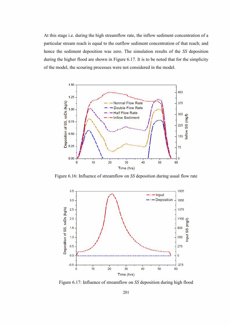
201

At this stage i.e. during the high streamflow rate, the inflow sediment concentration of a

particular stream reach is equal to the outflow sediment concentration of that reach; and

hence the sediment deposition was zero. The simulation results of the SS deposition

during the higher flood are shown in Figure 6.17. It is to be noted that for the simplicity

of the model, the scouring processes were not considered in the model.

Figure 6.16: Influence of streamflow on SS deposition during usual flow rate

Figure 6.17: Influence of streamflow on SS deposition during high flood

202

6.4.2.2 Influence of Inflow Sediment Concentration

The amount of sediment transferred from a particular catchment during storm events is

another important factor for the SS transportation within stream reaches. The general

trend for the SS transportation and deposition relies on the inflow sediment

concentration coming from contributed catchments to stream. van Rijn (1986) found a

large inaccuracy in the determination/assumption of the incoming sediment

concentration used as boundary conditions at the inlet. Therefore, an accurate estimation

of the inflow sediment concentration is essential. To demonstrate the influence of

incoming SS, the model was simulated with the three different inflow concentrations at

a particular stream reach. The plotted results of the SS transportation and deposition

rates are shown in Figures 6.18 and 6.19 respectively.

Figure 6.18: The influence of incoming SS concentrations on transportation

Figure 6.18 shows the variations of the simulated results for the transportation of SS

through a particular stream section with the selected varying inflow sediment

concentrations. From the figure, for this particular condition, it was found that the

transport rate of SS was the same even if the incoming sediment concentrations were

double. This supports the fact that the transport rate of SS from a particular stream reach

for a particular flow rate depends on the transport capacity of that section, i.e. the stream

203

has a maximum capacity to transport SS to the downstream. Where the concentration of

SS is more than the transport capacity of the stream, SS is deposited onto the stream bed.

Figure 6.19 illustrates the variations of SS deposition for that particular section. The

influence in the SS deposition appears to be large especially during the rising and falling

limb of the hydrographs. From Figure 6.19, it is clear that when the incoming sediment

concentration was higher, the deposition rate was higher. For very low concentration of

the incoming sediment, there was no deposition, i.e. all the sediments were transported

to the downstream. It should be noted that the streamflow was the same for all the three

different inflow sediment concentrations.

Figure 6.19: The influence of the incoming SS concentration on deposition

6.4.2.3 Influence of Median Particle Diameter

The median particle diameter (D50) is one of the most important factors in the

transportation and deposition of SS. van Rijn (2007) found that the transportation of SS

is strongly related to the particle size. Nicholas and Walling (1998) also noted that the

deposition rate is strongly controlled by the particle fall velocity, which is usually

determined from D50. In most of the practical cases, data for D90 is not readily available,

so it is determined from D50. To show the variations of D50 on the SS processes in a

particular stream section, the model was simulated with different D50.

204

Figure 6.20: The influence of D50 on SS transportation

Figure 6.21: The influence of D50 on SS deposition

The graphical presentation of these variations is shown in Figures 6.20 and 6.21 for SS

transportation and deposition respectively. Figure 6.20 demonstrates the variations of

the transport rate with the variations of D50. The figure reveals that the transport rate

increases with decreased D50 and decreases with increased D50. However, the rate of

deposition increases with increased D50 and decreases with decreased D50.

205

When D50 increases, particle fall velocity will increase, which helps to deposit more

particles on the stream bed. However, these variations were not even. Figure 6.21 shows

the variations of the deposition rate with the variations of D50. From the figure, it is

clear that the size of sediment particles significantly impacts upon the deposition rate.

Hence, the field measurement of the particle size is extremely important for the better

prediction of the SS transport and deposition rate.

6.4.2.4 Influence of Particle Density

Density of the particles has a considerable influence on the particle fall velocity which

is another most influential parameter of the SS processes. Hence, the determination of

the effects of sediment density on the SS processes is essential. To illustrate the

influence of sediment density on the SS processes, the model was simulated with

varying sediment densities; while the inflow sediment concentration was the same. The

simulated results of the variations are shown in Figures 6.22 and 6.23 for the transport

and deposition rates respectively. Figure 6.22 illustrates the transport rate of SS with the

three different sediment densities. The figure reveals the obvious phenomena that

transportation of SS is sensitive to the density of the particles. From Figure 6.22 and

Table 6.7, it is clear that an increase in sediment density by 25% decreased the transport

rate by up to 50% during the peak flow.

Figure 6.22: The influence of sediment density on SS transportation

206

On the other hand, decrease in sediment density by 25% increased the transport peak by

about only 30%. Figure 6.22 shows the plotted results of the SS deposition rate with the

three different sediment densities. It is clear from the figure that similar to the transport

rate, the deposition of SS was also sensitive to the density of the sediment particles. If

the sediment density went much lower, there was no SS deposition, i.e. all the sediment

was transported to the downstream. However, those outcomes will largely depend on

the other parameters, such as streamflow, D50, water temperature etc. In general, the SS

processes are highly depended on the particle density and its field measurement is

highly important.

Figure 6.23: The influence of sediment density on SS deposition

6.4.2.5 Influence of Water Temperature

Water temperature is also another important parameter in determining the transport and

deposition rate of SS. With the increase in water temperature, water density reduces

causing an increase in sediment fall velocity. Figures 6.24 and 6.25 show the influence

of water temperature on the SS processes. Figure 6.24 demonstrates the variations of SS

transportation with the temperature which represents the obvious phenomena that the

transport rate decreases with increasing temperature and increases with decreasing

temperature. From Figure 6.24 and Table 6.7, it was found that the peak transport rate

varies more than 7% for a temperature variation of 100%.

207

Figure 6.24: Effects of the temperatures on SS transportation

Figure 6.25: Effects of the temperatures on SS deposition

Figure 6.25 demonstrates the sensitivity of SS deposition with the temperature

variations. From Figure 6.25, it is clear that the deposition rate increases with increasing

temperature and decreases with decreasing temperature. From the detailed analysis, it

was also observed that the change in the peak sediment transport and deposition was

linear with the temperature variations. Hence, an accurate measurement of water

temperature will increase the accuracy of model predictions.

208

6.4.3 Sensitivity of TN and TP Parameters

Although the modelling processes of TN and TP are widely used in water quality

modelling, there is the lack of systematic testing of sensitivities of the rate parameters.

In this research, the sensitivity of the developed model was undertaken to improve

understanding of the behaviour of the developed model. This information will be used

to simplify and improve the model structure and parameterisation where possible. The

factor screening sensitivity measure was used to assess the impact of the perturbations

of the model parameters.

The sensitivity of the rate parameters of the reactive pollutants (TN and TP) for the

stream water quality model was identified in terms of the PBIAS and NSE values. The

summary results for sensitivity analysis of the rate parameters are shown in Tables 6.8

and 6.9. Table 6.8 shows the sensitivity results of PBIAS values; while Table 6.9 shows

the sensitivity results of NSE values.

Table 6.8 reveals that in terms of the PBIAS values, the output of the TN processes were

more sensitive to the perturbation of the coefficient for mineralisation of TN from BOD

(kTN), and less sensitive to the denitrification coefficient (kDEN) and release rate of TN

from sediment (ksTN). There was no change in the PBIAS values due to the perturbation

of kDEN as shown in Table 6.8. The initial value of kDEN was assumed based on published

literature which considered only a fragment of nitrogen instead of TN.

Table 6.8: Sensitivity of PBIAS values of the rate parameters for TN and TP


-10.00%

Perturbation

-5.00%

Perturbation

0.00%

Perturbation

+5.00%

Perturbation

+10.00%

kBOD 0.001 0.0002 0.000 0.0003 0.001

kDEN 0.000 0.000 0.000 0.000 0.000

kTN 0.092 0.0432 0.000 0.041 0.029

ksTN 0.000 0.000 0.000 0.000 0.000

kTP 0.233 0.104 0.000 -0.086 -0.159

ksTP 0.000 0.000 0.000 0.000 0.000

δTP -0.845 -0.043 0.000 0.050 0.102

209

Similar to kDEN, there was no change in the PBIAS values due to the perturbation of ksTN.

This was reasonable because the considered stream was shallow in depth and there was

no deposited sediment to release TN during the simulation period. Table 6.8 also reveals

that the predicted values of the TP processes were more sensitive to the perturbation of

the adjustment factor for sediment TP release (δTP) and to the coefficient for

mineralisation of TP from BOD (kTP); and less sensitive to the release rate of TP from

sediment (ksTP) in terms of the PBIAS values. However, kTP and δTP are interrelated

because both of these parameters are associated with sediment TP release. Hence, all of

the parameters should be estimated with great care from the observed field data.

Table 6.9: Sensitivity of NSE values of the rate parameters for TN and TP


-10.00%

Perturbation

-5.00%

Perturbation

0.00%

Perturbation

+5.00%

Perturbation

+10.00%

kBOD 1.000 1.000 1.000 1.000 0.999

kDEN 1.000 1.000 1.000 1.000 1.000

kTN 0.991 0.998 1.000 0.998 0.957

ksTN 1.000 1.000 1.000 1.000 1.000

kTP 0.976 0.994 1.000 0.994 1.068

ksTP 1.000 1.000 1.000 1.000 1.000

δTP 0.996 0.999 1.000 0.999 0.975

Table 6.9 shows the sensitivity of the rate parameters of TN and TP in terms of NSE

values for the estimated parameters of Saltwater Creek. From the table, it is clear that

for all the perturbations, the NSE values were very close to 1.0 which contradicts with

the sensitivity of the PBIAS values. This contradiction reveals that the estimated

parameters may not be represented for the creek. It should be noted that due to the

limitations of measured data, the parameters were estimated only from a limited number

of observations. Furthermore, the perturbation of the model parameters was done based

on the estimated parameters of SWCC only. Hence, for the real time sensitivity, the

model parameters should be estimated from the adequate and reliable observed field

data.

210

6.4.3.1 Influence of Hydraulic Radius

The usual practice of the hydraulic radius is that it is assumed to be the depth of flow.

This assumption is quite good for wide channels where width of a stream channel is

much greater (BW > 5ht) than the depth of flow. However, for the streams with a small

width, this assumption will produce gross error. To reduce this error, the model was

developed by considering the hydraulic radius as a power function of the flow depth by

introducing the two new terms CFc and CFe. Figure 6.26 shows the simulation results

of SS for Saltwater Creek by considering it as having a wide channel and by estimating

CFc and CFe. The values of CFc and CFe were estimated from the calculated hydraulic

radius and flow data estimated by the HEC RAS model. From Figure 6.26, it is clear

that the transportation of SS was almost the same for both cases, i.e. when the channel

was wide as well as non-wide. Hence, someone might argue that the estimation of CFc

and CFe is useless. It is true for the streams where the SS transport capacity is higher,

i.e. when all the incoming sediment is transported to the downstream. However, for too

much incoming sediment concentration or for too low streamflow, there was sediment

deposition on the stream bed shown in the Figure 6.26. At this stage, the consideration

of the hydraulic radius equal to the flow depth produces gross error.

Figure 6.26.: The variation of hydraulic radius on SS transport

211

6.5 Conclusions Sensitivity analysis is an important component for evaluating the water quality

modelling techniques. This chapter presented the detailed sensitivity analysis of the

different parameters of the developed integrated catchment-stream water quality model.

The analysis was undertaken to assess sensitivity of individual parameter and to find out

the most sensitive parameter of the developed model. This analysis was required as a

part of an effort to increase understanding of a modeller’s knowledge about considered

processes in the model development and to provide a guide for shifting the scale of

model application.

Since the main purpose of sensitivity analysis of this chapter was to obtain a broader

feeling of sensitive parameters of the developed model, a simple sensitivity analysis

method (i.e. one at a time sensitivity analysis) was used. For this thesis the factor

screening approach was used which is useful for providing a guide for the future

assessment of the water quality model using a general sensitivity technique. Based on

the detailed analysis, the following conclusions were drawn.

By examining the expected direction of the changes in the model output, it can be

concluded that the model was coded correctly and behaved as expected. For example,

the model can simulate the phenomenon that increases in rainfall intensity and duration

does not always increase the pollutant wash-off rate rather it decreases with time from

the beginning. Also decrease in D50 of SS decreases the amount of deposition on the

stream bed. However, the transport rate would remain unaffected by the change in the

input SS due to the limited transport capacity of a particular streamflow rate.

From the sensitivity of the catchment water quality model, it was found that maximum

build-up rate is the most sensitive parameter of the pollutant build-up model. Another

sensitive parameter of this model is the build-up rate constant. On the other hand,

coefficients of both the power function wash-off model and the rating curve wash-off

model were more sensitive than exponents. Therefore, these coefficients should be

determined carefully from calibration. Moreover, it was observed that the pollutant

wash-off is dependent on the available pollutants of catchment surfaces. In addition,

sensitivity analysis indicated that multiple parameter sets can be derived from the

similar level of calibration.

212

The variability in the parameter values of the catchment water quality model suggests

that the generic application of the sophisticated build-up wash-off model should be

performed cautiously. Further research is needed to derive the appropriate values of the

build-up wash-off model parameters for the practical application with a greater degree

of confidence.

From sensitivity analysis of the stream water quality model, it can be concluded that the

overall accuracy of the SS processes is largely determined by the accuracy of boundary

conditions, such as the inflow concentration of SS coming from upstream catchments to

streams. The application of the model is hindered when the accurate boundary

conditions, such as field data is missing. In the absence of accurately measured

boundary conditions, the simulation leads to the biased results. The other influential

parameter of the model is the streamflow rate. From the sensitivity of the TN processes,

it was found that the mineralisation coefficient of TN (kTN) from BOD was the most

sensitive, and the denitrification coefficient (kDEN) was the least sensitive parameter. For

the TP processes, the most sensitive parameter was the adjustment factor (δTP) for

sediment TP release.

However, the accuracy of the model output responses were conducted based on limited

data. For the future sensitivity work of the developed model and similar variants, the

investigation of sensitivities across a range of spatial scales and sites is required. The

detailed field measurements are essential to specify the appropriate boundary

conditions, especially when an accurate morphological prediction is required. These

results have important implications for focusing the future research associated with the

developed model.

From the overall sensitivity analysis, it can be cautiously concluded that the developed

model is generally performing well at predicting the patterns of both discharge and

pollutant loads. Reference to this research will guide to the future sensitivity

assessment. Sensitivity analysis presented here could be extended potentially to gain

additional insight into the behaviour of the model. Further analysis is required before

more definitive conclusions can be reached. It will also help to determine the relative

importance of the model parameters involved in the modelling processes.

213

Chapter 7 Conclusions and Recommendations

7.1 Overview of the Study The primary objective of this research was to develop an integrated catchment-stream

water quality model which continuously simulates different water quality parameters.

The main aim was to assist watershed managers to establish improved management

strategies to protect aquatic environments from the impact of pollution. The procedure

of the developed model was based on the hypothesis that an integrated modelling

approach can be used to predict water quality parameters from both catchment and

stream reach together. The integrated approach was chosen for the model development

because single isolated models tend to predict the inconsistent and biased results.

This thesis explored the catchment and stream water quality modelling approaches

through a detailed literature review. The literature review identified that at that time

there were no integrated catchment-stream water quality model for the prediction of

water quality parameters. The review demonstrated the development, application and

testing processes of hydrology, hydraulics and water quality parameters. The research

achieved its three main aims:

A catchment water quality model was developed for the prediction of

stormwater pollutants SS, TN and TP, which are transported from upstream

catchments through a catchment outlet. This was achieved by firstly developing

a runoff model and then a pollutant model. The runoff model allows the

determination of CL using any of the available estimation methods (i.e. constant,

linearly varying or exponentially varying), rather than using a fixed rainfall loss

value for the duration of rainfall. The runoff modelling results were compared

with the estimated discharges from WBNM, DRAINS and MUSIC. Widely used

pollutants processes were refined and incorporated to estimate the export of

water quality parameters from catchment surfaces. The catchment water quality

model determines surface runoff and pollutant loads, and allows the estimation

214

of pollutants build-up during the dry periods and pollutants wash-off as a result

of rainfall events. The users have the options of choosing the best pollutant

build-up and wash-up model from various build-up and wash-off equations.

A stream water quality model was developed for the continuous simulation of

water quality parameters coming from upstream catchments to a stream reach.

This was performed by incorporating the stream dynamics and stream pollutants

processes. For the streamflow, a simple flow routing model (the Muskingum-

Cunge method) was used. The estimated flows of the developed model were

compared with the calculated flows from HEC RAS and MUSIC. The

techniques of SS and nutrients processes were refined, improved and

incorporated with the streamflow model.

An integration of the catchment water quality model with the stream water

quality model was performed to be able to continuously simulate different water

quality parameters. Incorporation of the integrated modelling technique of

catchment and stream water quality parameters is very useful for the prediction

of water borne pollutants.

In addition, to achieving the three main aims of this research, other important outcomes

were also achieved. After developing the basic model structure, it was proven that this

model could be adapted to catchments and streams, where complex models are not

suitable from the practical and economic point of view. The application of the integrated

model developed in this research has provided a capacity to quantify water quality

parameters.

The developed integrated water quality model, like other water quality models, needs

calibration to estimate the model parameters. For this estimation, the manual calibration

procedure was used in this study. The method was used to provide the best set of model

parameters that considers several storm events simultaneously. For calibration and

validation of the integrated model, different published data and reliable source (GCCC)

data were used. Rainfall data was collected from the nearby meteorological station

‘Gold Coast Seaway’. The catchment characteristics data was obtained from the land-

use maps, contour maps and aerial photographs of the area.

215

The experimental water quality data was collected from the available literature for the

two impervious surfaces, i.e. road and roof surfaces. Field measurement water quality

data was collected for the two catchments, i.e. HTCC and SWCC, which are located at

Gold Coast, Australia. These two catchments represent typical small and medium

watershed areas in Gold Coast. The initial values of the model parameters were also

obtained from the available literature. Since catchment water borne pollutants are

generated from impervious and/or pervious areas, the parameters of the catchment water

quality model were determined for both impervious and pervious areas separately.

Calibration of the stream water quality model was also performed for the Gold Coast

area. The parameters of this model were determined from an 1825 m long reach section

of Saltwater Creek. The parameters of the Muskingum-Cunge routing technique and

pollutants processes were determined separately for the creek.

Finally, the calibrated model parameters, the catchment and stream characteristics were

used to assess sensitivity of the model parameters on the simulated hydrographs and

pollutographs. This model extends beyond the previous efforts in the area of dynamic

water quality modelling approaches and proposes a method for generating a reliable

estimation of water quality parameters. The factor screening sensitivity analysis

technique was used for this study.

This research into the integrated water quality model enhances the current knowledge

about isolated water quality models and provides a direction in further development of

integrated models. Furthermore, this research contributes towards the effective design of

water quality mitigation strategies for the protection and improvement of aquatic

environments and ecosystems from the impact of water pollution.

7.2 Conclusions This thesis made a number of contributions to the development of an integrated water

quality modelling technique for the purpose of improving management of aquatic

environments. The goal of the approach was to reduce the complexity and effort using

several individual modelling approaches to compute and analyse water quality

parameters. The integrated model was tested for the widespread application to

catchments and streams with the same physical environments and constraints.

216

The catchment water quality model can account for the fact that CL not only remain

constant for the whole duration of a storm event but also decreases with time. The

phenomena of non-point pollutant build-up and wash-off are influenced by a large

number of factors and their dynamics are still not well-known. Based on the analysis of

the modelling output, the model parameters should be estimated through the calibration

procedure using field measurements for a specific area for several continuous storm

events, instead of a single rainfall event. The catchment water quality model provides

fairly accurate field data when correctly calibrated with the observed data. It is therefore

reasonable to conclude that the developed model can be applied to any catchment in

Australia and throughout the world, provided the proper values of the model parameters

are selected. The model allows the users to specify time step for both the hydrograph

and pollutograph simulation.

The stream water quality model introduced a new technique for the calculation of the

hydraulic radius of a particular stream reach instead of taking it equal to the depth of

flow. This method of the hydraulic radius calculation is very useful method for water

engineering practices. The proposed SS transport model yields the reliable results in the

prediction of the sediment concentration, transportation and deposition. The method was

applied to estimate the suspended sediment transportation and deposition, and provided

fairly accurate prediction results comparing with the usual methods.

Comparing the modelling results with the commercially used models, it was found that

this model produces the similar results. It can therefore be concluded that the proposed

technique is promising and may be beneficial to overcome the burden of using

individual models. The model will help to provide guidelines not only to resource

managers in restoring aquatic ecosystems, but also to local planners devising viable and

ecologically sound watershed development plans as well as for policy makers in

evaluating alternate land management decisions. The outcomes of the study suggest that

the model is a potential tool which will aid in the development of management

strategies for complex watershed areas. The model can be used to generate scenarios as

a part of a general strategy to conserve or improve the quality of water. The developed

model and similar variants have much potential to predict water quality parameters of

an aquatic environment.

217

Both the catchment water quality model and the stream water quality model have

complexity commensurate with data availability and the potential for the widespread

application. The disadvantage of the model is the need for the accurate field

measurement data to calibrate the model parameters. There is also a loss of accuracy,

because of unsophisticated representation of the physics of the relevant modelling

processes. Another disadvantage is that the model does not consider the cohesive

properties of SS particles, such as flocculation, consolidation and fluidisation. These

processes were ignored in order to make the model user friendly.

The calibrated model responses and sensitivities are in agreement with the observed

water quality data. Since some of the model parameters are interrelated with each other,

it is difficult to find out the most sensitive parameter of the model. However, the major

conclusion reached through the sensitivity assessment was that boundary conditions of

the developed model are the most sensitive. Hence, the investigation to the boundary

conditions should be the initial focus in the practical application of the model and its

improvement.

The integrated model which has been developed can be used to assess the effectiveness

of management decisions about catchments and streams. The output will provide useful

data for decision making about existing wastewater treatment plants and/or controlling

the non-point source pollutant loadings.

Finally, by replacing the earlier forms of system modelling, the integrated assessment

and modelling of water quality parameters will facilitate scenario generation and

decision support functions. Further development of this integrated water quality model

could eliminate the inconsistent results arising from the isolated models.

7.3 Recommendations and Future Research It is expected that there are spatial variations of rainfall within a particular catchment

especially for large rainfall events. The model allows the users to consider data only

from one rainfall station. Therefore, this model should be further developed to include

the spatial variations of rainfall to make a more accurate prediction of water quality

parameters.

218

It was hypothesised that the characteristics of the influential variables are fairly constant

over the studied catchments. The future research should investigate the model

parameters for the variable catchment characteristics.

The current catchment water quality model did not consider the BOD process which is

one of the main pollutants of streams. For an accurate estimation of BOD within a

particular stream, the BOD process should be incorporated with the catchment water

quality model.

It should be noted that the estimation of the model parameters in this research was

performed with only a limited number of observations. Therefore, further tests of the

model are most desirable using more experimental and observed field data. This model

was calibrated only for data from Gold Coast. It is suggested that further calibration

with data from other catchments in different regions be performed so that a ranged

values of the model parameters can be established.

Furthermore, sensitivity of the model parameters was performed by considering the

calibrated parameters as optimal. However, the parameters were estimated only with a

limited number of observed data as mentioned earlier. Therefore, future investigation of

sensitivity analysis needs to be directed across a wide range of spatial scales and sites.

Moreover, examination of model sensitivity should be performed by considering the

correlation structure of the model parameters to increase the better understanding of the

model users.

In addition, as this model does not take into the consideration of economic aspects of

management changes, this should be incorporated as a part of pollutant load model to

further assist in prioritising management expenditure. The model also does not identify

the relationship between the Manning’s ‘n’ value and the Muskingum-Cunge method.

The relationship needs to be established in the future.

219

Bibliography

Adams, B.J. and Papa, F. (2000). Urban stormwater management planning with analytical

probabilistic models. John Willey and Sons: New York.

Ahyerre, M., Chebbo, G., Tassin, B., Gaume, E. (1998). Storm water quality modelling, an

ambitious objective? Water Science and Technology, 37(1): pp. 205-213.

Akan, A.O. and Houghtalen, R.J. (2003). Urban hydrology, hydraulics, and stormwater quality-

Engineering applications and computer modelling, New Jersey, John Willey and Sons,

Inc.

Akan, A.O. (1987). Pollutant Wash-off by overland flow. Journal of Environmental

Engineering, 113(4): pp. 811-823.

Ali, A.M., Yusoff, C.F.C.M. and Musa, S. (2010). Determination of sediment transport at river

system. Proceedings of the 3rd International Conference on Southeast Asian Natural

Resources and Environmental Management (SANREM) Conference, 3-5 August 2010,

Kota Kinabalu, Sabah, Malaysia.

Allison, R.A., Chiew, F.H.S. and McMahon, T.A. (1998). Nutrient contribution of leaf litter in

urban stormwater. Journal of Environmental Management, 54(4): pp. 269-272.

Alley, W.M. (1981). Estimation of impervious-area wash-off parameters. Water Resources,

17(4): pp. 1161-1166.

Alley, W.M. and Smith, P.E. (1981). Estimation of accumulation parameters for urban runoff

quality modelling. Water Resources, 17(6), pp. 1657-64.

Amoudry, L. (2008). A review on coastal sediment transport modelling. Proudman

Oceanographic Laboratory, UK. Internal Document No. 189.

Armitage, N. and Rooseboom, A. (2000). The removal of urban litter from stormwater conduits

and streams: Paper 1- The quantities involved and catchment litter management options.

Water SA, 26(2): pp. 181-188.

Bach, P.M., McCarthy, D.T. and Deletic, A. (2010). The development of a novel approach for

assessment of the first flush in urban stormwater discharges. Water Science and

Technology, 61(10): pp. 2681-2688.

220

Bagnold, R.A. (1966). An approach to the sediment transport problem from general physics.

Geological Survey Professional Paper No. 422-I, U.S. Government Printing Office,

Washington, D.C.

Ball, J.E., Wojcik, A. and Tilley, J. (2000). Stormwater quality from road surfaces- Monitoring

of the Hume Highway at South Strathfield. The University of New South Wales, School

of Civil and Environment Engineering, Water Research Laboratory, Research Report 204.

Ball, I.E., Jenks, R. and Aubourg, D. (1998). An assessment of the availability of pollutant

constituents on road surfaces. Science of the Total Environment, 209(2-3): pp. 243-254.

Ballo, S., Liu, M., Hou, L. and Chang, J. (2009). Pollutants in stormwater runoff Shanghai

(China): Implications for management urban runoff pollution. Progress in Natural

Science, 19(7): pp. 873-880.

Bannerman, R.T., Owens, D.W., Dodds, R.B. and Hornewer, N.J. (1993). Sources of pollutants

in Wisconsin stormwater. Water Science and Technology, 28(3-5): pp. 241-259.

Barbe, D.E., Cruise, J.F. and Mo, X. (1996). Modelling the build-up and washoff pollutants on

urban watersheds. Water Resource Bulletin AWRA, 32(3): pp. 511-519.

Barry, D.A. and Bajracharya, K. (1995). On the Muskingum-Cunge flood routing method.

Environment International, 21(5): pp. 485-490.

Baffaut, C. and Delleur, J.W. (1990). Calibration of SWMM runoff quality model with expert

system. Journal of Water Resources Planning and Management, 116(2): pp. 247-261.

Batroney, T., Wadzuk, B.M. and Traver, R.G. (2010). Parking deck’s first flush. Journal of

Hydrologic Engineering, 15(2): pp. 123-128.

Beck, M.B. (1991). Principles of modelling. Water Science and Technology, 24(6): pp. 1-8.

Benfer, N.P., King, B.A. and Lemckert, C.J. (2007). Salinity observations in a subtropical

estuarine system on the Gold Coast, Australia. Journal of Coastal Research, Special Issue,

50: pp. 646-651.

Beres, D.L. and Hawkins, D.M. (2001). Plackett-burman technique for sensitivity analysis of

many parameters model. Ecological Modelling, 141(1-3): pp. 171-183.

Berretta, C., Gnecco, I., Lanza, L.G. and La Barbara, P. (2007). An investigation of wash-off

controlling parameters at urban and commercial monitoring sites. Water Science and

Technology, 56(12): pp. 77-84.

221

Bertrand-Krajewski, J.L., Scrivener, O. and Briat, P. (1993). Sewer sediment production and

transport modelling: A literature review. Journal of Hydraulic Research, 31(4): pp. 435-

460.

Beven, K. and Binley, A. (1992). The future of distributed models: model calibration and

uncertainty prediction. Hydrological Processes, 6(3): pp. 279-298.

Bilotta, G.S. and Brazier, R.E. (2008). Understanding the influence of suspended solids on

water quality and aquatic biota. Water Research, 42(12): pp. 2849-2861.

Bohemen, H.D. and De Laak, W.H.J.V. (2003). The influence of road infrastructure and traffic

on soil, water and air quality. Environmental Management, 31(1): pp. 50-68.

Boorman, D.B. (2003). LOIS in-stream water quality modelling. Part 1. Catchments and

methods. The Science of the Total Environment, 314-316, pp. 379-395.

Boughton, W. and Droop, O. (2003). Continuous simulation of design flood estimation – a

review. Environmental Modelling and Software, 18(4): pp. 309-318.

Bouteligier, R., Vase, G. and Berlamont, J. (2002). Sensitivity of urban drainage wash-off

models: compatibility analysis of hydroworks QM and MouseTrap using CDF

relationships. Journal of Hydroinformatics, 4(4): pp. 235-243.

Bowie, G.L., Mills, W.B., Porcella, D.B., Campbell, C.L., Pagenkopf, J.R., Rupp, G.L.,

Johnson, K.M., Chan, P.W.H. and Gherini, S.A. (1985). Rates, constants, and kinetics

formulations in surface water quality modelling (second edition). Report EPA/600/3-

85/040. U.S. EPA, Athens, Georgia 30613.

Brezonik, P.L. and Stadelmann, T.H. (2002). Analysis and predictive models of stormwater

runoff volumes, loads and pollutant concentrations from watersheds in the twin cities

metropolitan areas Minnesota, USA. Water Research, 36(7): pp. 1743-1757.

Brinkmann, W.L.F. (1985). Urban stormwater pollutants: Sources and loadings. Geo Journal,

11(3): pp. 277-283.

Brown, L.C. and Barnwell, T.O. (1987). The enhanced stream water quality models QUAL2E

and QUAL2E-UNCAS: documentation and user manual. Report EPA/600/3-87/007. U.S.

EPA, Athens, Georgia 30613.

Butcher, J.B. (2003). Buildup, washoff, and event mean concentrations. Journal of the American

Water Resources Association, 39(6): pp. 1521-1528.

222

Butcher, D.P., Labadz, J.C., Potter, A.W.R., White, P., (1993). Reservoir sedimentation rates in

the Southern Pennine region, UK. In: McManus, J., Duck, R.W. (Eds.), Geomorphology

and Sedimentology of Lakes and Reservoirs. Wiley, Chichester, pp. 73–93.

Byun, D., Cho, Y., Huh, I., and Hart, D.E. (2005). Runoff-induced vertical thermal dynamics in

a canyon-shaped reservoir during the summer monsoon. Marine and Freshwater Research

56(7), pp. 959–968.

Carpenter, S.R., Caraco, N.F., Correl, D.L., Howarth, R.W., Sharpley, A.N. and Smith, V.H.

(1998). Nonpoint pollution of surface waters with phosphorus and nitrogen. Issues in

Ecology, 8(3): pp. 559-568.

Celik, I. and Rodi, W. (1989). Modelling suspended sediment transport in nonequilibrium

situations. Journal of Hydraulic Engineering, 114(10): pp.1157-1191.

Chang, C.L., Lo, S.L. and Chen, M.Y. (2007). Uncertainty in watershed response predictions

induced by spatial variability of precipitation. Environmental Monitoring and

Assessment, 127(1-3): pp. 147-153.

Chapra, S.C. (1997). Surface water-quality modeling. McGraw-Hill, New York.

Charbeneau, R.J. and Barrett, M.E. (1998). Evaluation of methods for estimating stormwater

pollutant loads. Water Environment Research, 70(7): pp. 1295-1302.

Chaubey, I., Haan, C.T., Grunwald, S. and Salisbury, J.M. (1999). Uncertainty in the model

parameters due to spatial variability of rainfall. Journal of Hydrology, 220(1-2): pp. 48-

61.

Cheah, C.H. and Ball, J.E. (2007). An alternative approach to modelling stormwater runoff from

small urban catchment. International Journal of Water, 3(4): pp. 322-333.

Chen, J. and Adams, B.J. (2007). A derived probability distribution approach to stormwater

quality modelling. Advance in Water Resources, 30(1): pp. 80-100.

Chen, J. and Adams, B.J. (2006). Analytical urban storm water quality models based on

pollutant buildup and washoff process. Journal of Environmental Engineering, 132(10):

pp. 1314-1330.

Chiew, F.H.S. and McMahon, T.A. (1999). Modelling runoff and diffuse pollution loads in

urban areas. Water Science and Technology, 39(12): pp. 241-248.

Chiew, F.H.S. and McMahon, T.A. (1997). Modelling daily runoff and pollutant loads from

urban catchments. Water (AWWA) Journal, 24: pp. 16-17.

223

Chow, V.T. (1959). Open channel hydraulics. McGraw-Hill Book Company, Inc, New York.

Christophersen, N and Wright, R.R. (1981). Sulfate budget and a model for sulfate

concentration in stream water at Birkenes, a small forested catchment in southern

Norway. Water Resources Research, 17: pp. 377-389.

Chui, P.C. (1997). Characteristics of stormwater quality from two urban watersheds in

Singapore. Environmental Modeling and Assessment, 44: pp. 173-181.

CMU (Catchment Management Unit) (2002). Health of the Gold Coast Waterways. Gold Coast

City Council (GCCC) 2002 Report, Gold Coast, Australia.

Coleman, N.L. (1970). Flume studies of the sediment transfer coefficient. Water Resources,

6(3): pp. 801-809.

Campolongo, F., Saltelli, A., Sorensen, T. and Tarantola, S. (2000). Hitchhiker’s Guide to

Sensitivity Analysis. In: Sensitivity Analysis, Saltelli, A., Chan, K. and Scott, E.M. eds,

pp. 15-50, John Willey and Sons, Ltd., Chichester.

Cowen, W.F. and Lee, G.F. (1973). Leaves as a source of phosphorus. Environmental Science

and Technology, 7(9): pp. 853-854.

Cox, B.A. (2003). A review of currently available in-stream water-quality models and their

applicability for simulating dissolved oxygen in lowland rivers. Science of the Total

Environment, 314-316: pp. 335-377.

CRC for Catchment Hydrology (2005). MUSIC (Model for urban stormwater improvement

conceptualization), Version 3, User Manual. Cooperative Research Centre for Catchment

Hydrology, Melbourne, Australia.

Cunge, J.A. (1969). On the subject of flood propagation computation method (Muskingum

method). Journal of Hydraulic Research, 7(2): pp. 205-230.

Dai, J.J., Lorenzato, S. and Rocke, D.M. (2004). A knowledge-based model of watershed

assessment for sediment. Environmental Modelling and Software, 19(4): pp. 423-433.

Daniels, R.B. and Gilliam, J.W. (1996). Sediment and chemical load reduction by grass and

riparian filters. Soil Science Society of America Journal, 60(1): pp. 246-251.

Datry, T., Malard, F., Vitry, L., Hervant, F. and Gibert, J. (2003). Solute dynamics in the bed

sediments of a stormwater infiltration basin. Journal of Hydrology, 273(1-4): pp. 217-

233.

224

Davis, B.S. and Birch, G.F. (2009). Catchment-wide assessment of the cost-effectiveness of

stormwater remediation measures in urban areas. Environmental Science and Policy,

12(1): pp. 84-91.

Davis, A.P, Shokouhian, M. and Ni, S. (2001). Loading estimates of Lead, Copper, Cadmium

and Zinc in urban runoff from specific sources. Chemosphere, 44(5): pp. 997-1009.

Dayaratne, S.T. (2000). Modelling of urban stormwater drainage system using ILSAX. PhD

Thesis, Victoria University of Technology.

Deksissa, T., Meirlaen, J., Ashton, P.J. and Vanrolleghem, P.A. (2004). Simplifying dynamic

river water quality modelling: A case study of inorganic nitrogen dynamics in the

Crocodile River (South Africa). Water, Air, and Soil Pollution. 155(1-4): pp. 303-320.

Deletic, A. (2005). Sediment transport in urban runoff over grassed areas. Journal of Hydrology,

301(1-4): pp. 108-122.

Deletic, A. and Orr, D.W. (2005). Pollution build-up on road surfaces. Journal of Environmental

Engineering, 131(1): pp. 49-59.

Deletic, A. (2001). Modelling of water and sediment transport over grassed areas. Journal of

Hydrology, 248(1-4): pp. 168-182.

Deletic, A. (1998). The first flush load of urban surface runoff. Water Research, 32(8): pp.

2462-2470.

Deletic, A.B. and Maksimovic, C.T. (1998). Evaluation of water quality factors in storm runoff

from paved areas. Journal of Environmental Engineering, 124(9): pp. 869-879.

Deletic, A.B., Maksimovic, C.T. and Ivetic, M. (1997). Modelling stormwater wash-off of

suspended solids from impervious surfaces. Journal of Hydrological Resources, 35(1): pp.

99-117.

DERM (Department of Environment and Resource Management) (2009). Gold Coast resource

operations plan, Gold Coast, Australia.

Dorney, J.R. (1986). Leachable and total phosphorus in urban street trees leaves. Water, Air and

Soil Pollution, 28(3-4): pp. 439-443.

Drapper, D., Tomlinson, R.M. and Williams, P. (2000). Pollutant concentrations in road runoff:

Southeast Queensland case study. Journal of Environmental Engineering, 126(4): pp.

313-320.

225

Drewry, J.J., Newham, L.T.H., Greene, R.S.B., Jakeman, A.J. and Croke, B.F.W. (2006). A

review of nitrogen and phosphorus export to waterways: Context for catchment

modelling. Journal of Marine and Freshwater Research, 58: pp. 757-774.

Duncan, H. (1999). Urban stormwater quality: A statistical overview (Report 99/3). Cooperative

Research Centre for Catchment Hydrology, Melbourne, Australia.

Eatherall, A., Boorman, D.B., Williams, R.J., Kowe, R. (1998). Modelling in-stream water

quality in LOIS. Science of the Total Environment, 24(210-211): pp. 499–517.

Egodawatta, P., Thomas, E. and Goonetilleke, A. (2009). Understanding the physical processes

of pollutant build-up and wash-off on roof surfaces. Science of the total environment,

407: pp. 1834-1841.

Egodawatta, P. and Goonetilleke, A. (2008). Understanding road surface pollutant wash-off and

underlying physical processes using simulated rainfall. Water Science and Technology,

57(8): pp. 1241-1246.

Egodawatta, P., Thomas, E. and Goonetilleke, A. (2007). Mathematical interpretation of

pollutant wash-off from urban road surfaces using simulated rainfall. Water Research,

41(13): pp. 3025-3031.

Egodawatta, P. (2007). Translation of small-plot scale pollutant build-up and wash-off

measurements to urban catchment scale. PhD Thesis: Faculty of Build Environment and

Engineering, Queensland University of Technology, Brisbane, Australia.

Elmore H.L. and Hayes T.W. (1960). Solubility of atmospheric oxygen in water. Journal of

Sanitary Engineering Division, 86(SA4), pp. 41–53.

Fang, X; Thompson, D.B.; Cleveland, T.G.; Pradhan, P. and Malla, R. (2008). Time of

concentration estimated using watershed parameters determined by automated and

manual methods. Journal of Irrigation and Drainage Engineering, 134(2): pp. 202-211.

Fang, X; Thompson, D.B.; Cleveland, T.G. and Pradhan, P. (2007). Variations of time of

concentration estimates using NRCS velocity method. Journal of Irrigation and Drainage

Engineering, 133(4): pp. 314-322.

Fergusson, J.E. and Ryan, D. (1984). The elemental composition of street dust from large and

small urban areas related to city type, source and particle size. Science of the total

Environment, 34(1-2): pp. 101-116.

226

Fletcher, T.D. and Deletic, A. (2007). Statistical evaluation and optimisation of stormwater

quality monitoring programmes. Water Science and Technology, 56(12): pp. 1-9.

Forster, J. (1996). Patterns of roof runoff contamination and their potential implications on

practice and regulation of treatment and local infiltration. Water Science and Technology,

33(6): pp. 39-48.

Fulazzaky, M.A., Seong, T.W. and Masirin, M.I.M. (2010). Assessment of water quality status

for the Selangor River in Malaysia. Water, Air, and Soil Pollution, 205(1-4): pp. 63-77.

Garcia, M.H. (2008). Sedimentation Engineering: Processes, measurements, modelling and

practice. ASCE Manuals and Reports on Engineering Practice No. 110. American Society

of Civil Engineers.

Garcia, M. and Parker, G. (1991). Entrainment of bed sediment into suspension. Journal of

Hydraulic Engineering, 117(4): p. 414-435.

Garde, R.J. and Raju, K.J.R. (2000). Mechanics of sediment transportation and alluvial stream

problems. New Age International Limited, New Delhi.

Garg, S.K. (2001). Irrigation engineering and hydraulic structures, Khanna Publishers, New

Delhi, India.

Gaume, E., Villeneuve, J.P. and Desbordes, M. (1998). Uncertainty assessment and analysis of

the calibrated parameter values of an urban storm water quality model. Journal of

Hydrology, 210: pp. 38-50.

Gavine, F., Gardener, T. and Carlin, G. (2000). Impact of acid sulphate soils on river water

quality in South East Queensland. Proceedings of the 3rd Queensland Environmental

Conference, Queensland, Brisbane, Australia, pp.209-217.

GCCC-Web (2010). Gold Coast City Council’s (GCCC) web page- www.goldcoast.qld.au

(08.08.2010).

Ghafouri, M. and Swain, C. (2004). Spatial analysis of urban stormwater quality. Journal of

Spatial Hydrology 5(1): pp. 33–46.

Glavan, M., White, S. and Holman, I.P. (2011). Evaluation of river water quality simulations at

a daily time-step- Experience with SWAT in the Axe catchment, UK. Clean- Soil, Air,

Water, 19(1): pp. 43-54.

Gobel, P., Dierkes, C. and Coldewey, W.G. (2007). Stormwater runoff concentration matrix for

urban areas. Journal of Contaminant Hydrology, 91(1-2): pp. 26-42.

http://www.goldcoast.qld.au/

227

Goonetilleke, A. and Thomas, E. (2003). Water quality impacts of urbanisation: Evaluation of

current research. Unpublished Academic Exercise, Energy and Resource Management

Research Program, Centre for Built Environment and Engineering Research, Queensland

University of Technology: Brisbane.

Goonetilleke, A. (1998). Use of geographical information systems for hydrological evaluation

and urban planning. PhD Thesis, Queensland University of Technology, Brisbane.

Gribbin, J.E. (2007). Introduction to hydraulics and hydrology with applications for stormwater

management. 3rd ed. Clifton Park, N.Y: Thomas Delmar Learning.

Grottker, M. (1987). Runoff quality from a street with medium traffic loading. Science of the

Total Environment, 59: pp. 457-466.

Gupta, H.V., Sorooshian, S. and Yapo, P.O. (1999). Status of automatic calibration for

hydrologic models: Comparison with multilevel expert calibration. Journal of Hydrologic

Engineering, 4(2): pp. 135-143.

Henderson, F.M. (1966). Open channel flow. The Macmillan Company, New York.

Herngren, L., Goonektilleke, A. and Ayoko, G.A. (2006). Analysis of heavy metals in road-

deposited sediments. Analytica Chimica Acta, 571(2): pp. 270-278.

Herngren, L. (2005). Build-up and wash-off process kinetics of PAHs and heavy metals on

paved surfaces using simulated rainfall. PhD Thesis: Faculty of Build Environment and

Engineering, Queensland University of Technology, Brisbane, Australia.

Herngren, L., Goonektilleke, A. and Ayoko, G.A. (2005). Understanding heavy metal and

suspended solids relationships in urban stormwater using simulated rainfall. Journal of

Environmental Management, 76(2): pp. 149-158.

Hill, P., Mein, R. and Siriwardena, L. (1998). How much rainfall becomes runoff? Loss

modelling for flood estimation (Industry Report 98/5). Cooperative Research Centre for

Catchment Hydrology, Melbourne, Australia.

Hoffman, E.J., Latimer, J.S., Hunt, C.D., Mills, G.L., and Quinn, J.G. (1985). Stormwater

runoff from highways. Water, Air and Soil Pollution, 25(4): pp. 349-364.

Hoffman, E.J., Mills, G.L., Latimer, J.S. and Quinn, J.G. (1984). Urban runoff as a source of

polycyclic aromatic hydrocarbons to coastal waters. Environmental Science and

Technology, 18: pp. 580-587.

228

Hoorman, J., Hone, T., Sdman Jr. T., Dirksen, T., Iles, J. and Islam, K.R. (2008). Agricultural

impacts on lake and stream water quality in Grand lake St. Marys, Western Ohio. Water,

Air, and Soil Pollution, 193(1-4): pp. 309-322.

Huber, W.C. and Dickson, R.E. (1988). SWMM (Stormwater Management Model). Version 4,

User Manual, USEPA (US Environmental Protection Agency), Athens, G.A.

Ilahee, M. and Imteaz, M. A. (2009). Improved continuing losses estimation using initial loss-

continuing loss model for medium size rural catchments. American Journal of

Engineering and Applied Sciences, 2(4): pp. 796-803.

Ilahee, M. (2005). Modelling losses in flood estimation. School of Urban Development,

Queensland University of Technology, Queensland, Australia.

Institute of Engineers Australia (IEAust), (2001). Australian rainfall and runoff. Institute of

Engineers Australia.

Jakeman, A.J., Letcher, R.A. (2003). Integrated assessment and modelling: Features, principles

and examples for catchment management. Environmental Modelling and Software, 18(6):

pp. 491-501.

James, W. and Thompson, M.K. (1997). Contaminants from Four New Pervious and

Impervious Pavements in a Parking-lot. Advances in Modeling the Management of

Stormwater Impacts, 5: pp. 207-221.

Jartun, M., Ottesen, R.T., Steinnes, E. and Voldena, T. (2008). Runoff of particle bound

pollutants from urban impervious surfaces studied by analysis of sediments from

stormwater traps. Science of the total Environment, 396: pp. 147-163.

Jonathan, I.G. and Nelson, E.J. (2002). Calculation of time of concentration for hydrologic

design and analysis using geographic information system vector objects. Journal of

Hydroinformatics, 4(2): pp. 75-81

Karadurmus, E. and Berber, R. (2004). Dynamic simulation and parameter estimation in river

streams. Environmental Technology, 25(4): pp. 471-479.

Kelly, J. Thornton, I. and Simpson, P.R. (1996). Urban geochemistry: A study of the influence

of anthropogenic activity on the heavy metal content of soils in traditionally industrial

and non-industrial areas of Britain. Environmental Geochemistry, 11(1-2): pp. 363-370.

Kibler, D.F. (1982). Urban stormwater hydrology. American Geophysical Union, Washington

D.C.

229

Kim, L.H., Zoh, K.D., Jeong, S.M., Kayhanian, M. and Stenstrom, M.K. (2006). Estimating

pollutant mass accumulation on highways during dry periods. Journal of Environmental

Engineering, 132(9): pp. 985-993.

Kim, L.H., Kayhanian, M. and Stenstrom, M. (2004). Event mean concentration and loading of

litter from highways during storms. Science of the Total Environment, 330(1-3): pp. 101-

113.

Kokken, T., Koivusalo, H., Karvonen, T. and Lepisto, A. (1999). A semi-distributed approach to

rainfall-runoff modelling- aggregating responses from hydrologically similar areas.

International congress on Modelling and Simulation Proceedings. University of Waikato,

New Zealand, Modelling and Simulation Society of Australia and New Zealand Inc.

Kronvang, B., Behrendt, H., Andersen, H.E., Arheimer, B., Barr, A., Borgvang, S.A., Bouraoui,

F., Granlund, K., Grizzetti, B., Groenendijk, P., Schwaiger, E., Hejzlar, J., Hoffmann, L.,

Johnsson, H., Panagopoulos, Y., Lo Porto, A., Reisser, H., Schoumans, O., Anthony, S.,

Silgram, M., Venohr, M. and Larsen, S.E. (2009). Ensemble modelling of nutrient loads

and nutrient load partitioning in 17 European catchments. Journal of Environmental

Monitoring, 11(3): pp. 572-583.

Kull, D.W. and Feldman, A.D. (1998). Evolution of Clark’s unit graph method to spatially

distributed runoff. Journal of Hydrologic Engineering, 3(1): pp. 9-19.

Ladson, A. (2008). Hydrology: An Australian introduction. South Melbourne, Vic.: Oxford

University Press.

Laenen, A. and Dunnette, D.A. (1997). River quality: Dynamics and restoration. CRC Lewis,

Boca Raton, New York.

Latimer, J.S., Hoffman, E.J., Hoffman, G., Fasching, J.L. and Quinn, J.G. (1990). Sources of

petroleum hydrocarbons in urban water runoff. Water, Air and Soil Pollution, 52(1-2): pp.

1-21.

Lau, S. and Stenstrom, M.K. (2005). Metals and PAHs adsorbed to street particles. Water

Research, 39(17): pp. 4083-4092.

Lawrence, P. and Atkinson, E. (1998). Deposition of fine sediments in irrigation canals.

Irrigation and Drainage systems, 12(4): pp. 371-385.

Lee, J.H., Bang, K.W., Ketchum, L.H., Choe, J.S. and Yu, M.J. (2002). First flush analysis of

urban stormwater runoff. The Science of Total Environment, 293(1-3), pp. 163-175.

230

Lee, J.G. and Bang, K.W. (2000). Characterization of urban stormwater runoff. Water Research,

34(6): pp. 1773-1780.

Leinster, S. and Walden, W. (1999). The application of sophisticated stormwater quality

estimation techniques in Australian catchments- A Queensland case study. In: Water 99:

Joint Congress, Brisbane, Australia: pp. 589-595.

Lin, B. and Namin, M.M. (2005). Modelling suspended sediment transport using an integrated

numerical and ANNs model. Journal of Hydraulic Research, 43(3): pp. 302-310.

Lin, J. and Chen, S. (1998). The relationship between adsorption of heavy metal and organic

matter in river sediments. Environment International, 24(3): pp. 345-352.

Lindenschmidt, K. (2006). The effect of complexity on parameter sensitivity and model

uncertainty in river water quality modelling. Ecological Modelling, 190(1-2): pp. 72-86.

Line, D.E., White, N.M., Osmond, D.L., Jennings, G.D. and Mojonnier, C.B. (2002). Pollutant

export from various land uses in the upper Neuse river basin. Water Environment

Research, 74(1): pp. 100-108.

Line, D.E., Wu, J., Arnold, J.A., Jennings, G.D. and Rubin, A.R. (1997). Water quality of first

flush runoff from 20 industrial sites. Water Environment Research, 69(3): pp. 305-310.

Linsley, R.K., Franzini, J.B. and Freyberg, D.L. (1992). Water resources engineering. 4th

Edition, McGraw-Hill, Inc., New York.

Maidment, D.R. (1993). Handbook of hydrology. McGraw Hill, New York.

Mannina, G. and Viviani, G. (2010). A parsimonious dynamic model for river water quality

assessment. Water Science and Technology, 61(3): pp. 607-618.

Margerum, R.D. and Born, S.M. (1995). Integrated environmental management: moving from

theory to practice. Journal of Environmental Planning and Management 38 (3), pp. 371–

391.

Marsden, J.R., Pingry, D.E. and Whinston, A. (1973). Application of nonlinear programming to

water quality control. Water, Air, and Soil Pollution, 2(2): pp. 155-169.

Marsili-Libelli, S. and Giusti, E. (2008). Water quality modelling for small river basins.

Environmental Modelling and Software, 23: pp. 451-463.

Mathers, N.J., Nash, D.M. and Gangaiya. P. (2007). Nitrogen and phosphorus exports from high

rainfall zone cropping in Australia: Issues and opportunities for research. Journal of

Environmental Quality, 36: pp. 1551-1562.

231

McCuen, R.H., Wong, S.L., and Rawls, W.J. (1984). Estimating urban time of concentration.

Journal of Hydraulic Engineering, 110(7): pp. 887-904.

Merritt, W.S, Letcher and Jakeman A.J. (2003). A review of erosion and sediment transport

models. Environmental Modelling and Software, 18: pp. 761-799.

Metcalf and Eddy Inc. and Alto, P. (1971). Stormwater management model. USEPA:

Washington D.C.

Miguntanna, N.P. (2009). Nutrients build-up and wash-off processes in urban land uses. PhD

Thesis: Faculty of Build Environment and Engineering, Queensland University of

Technology, Brisbane, Australia.

Miller, J.R. (1997). The role of fluvial geomorphic processes in the dispersal of heavy metals

from mine sites. Journal of Geochemical Exploration, 58: p. 101-118.

Moriasi, D.N., Arnold, J.G., Van Liew, M.W., Bingner, R.L., Harmel, R.D. and Veith,

T.L. (2007). Model evaluation guidelines for systematic quantification of

accuracy in watershed simulations. Transactions of the American Society of

Agricultural and Biological Engineers (ASABE), 50(3): pp. 885-900.

MW-Web (2011). Melbourne Water web page- http://www.melbournewater.com.au,

(18.06.2011).

Nelson, E.J. and Booth, D.B. (2002). Sediment sources in urbanising mixed land-use watershed.

Journal of Hydrology, 264: pp. 51-68.

Newham, L.T.H. (2002). Catchment scale modelling of water quality and quantity. PhD Thesis:

The Australian National University.

Nicholas, A.P. and Walling, D.E. (1998). Numerical modelling of floodplain hydraulics and

suspended sediment transport and deposition. Hydrological Processes, 12(8): pp. 1339-

1355.

Nix, S.J., (1994). Urban Stormwater Modelling and Simulation. Lewis Publishers, Boca Raton.

Novotny, V. and Olem, H. (1994). Water Quality: Prevention, Identification, and Management

of Diffuse Pollution. Van Nostrand Reinhold, New York.

Novotny, V., Sung, H.M., Bannerman, R. and Baum, B. (1985). Estimating non point pollution

from small urban watersheds. Journal Water Pollution Control Federation, 57(4): pp. 339-

348.

232

Obropta, C.C. and Kardos, J.S. (2007). Review of urban stormwater quality models:

Deterministic, stochastic, and hybrid approaches. Journal of the American Water

Resources Association, 43(6): pp. 1508-1523.

O’Reagain, P.J., Brodie, J., Fraser, G., Bushell, J.J., Holloway, C.H., Faithful, J.W. and Haynes,

D. (2005). Nutrient loss and water quality under extensive grazing in the upper Burdekin

river catchment, North Queensland. Marine Pollution Bulletin, 51(1-4): pp. 37-50.

Osuch-Pajdzinska, E. and Zawilski, M. (1998). Model of storm sewer discharge. Journal of

Environmental Engineering. 124(7): pp. 593-599.

Owusu-Asante, Y. and Stephenson, D. (2006). Estimation of storm runoff loads based on

rainfall-related variables and power law models- Case study in Alexandra. Water SA,

32(2): pp. 137-143.

Parker, P., Letcher, R., Jakeman, A., Beck, M.B., Harris, G., Argent, R.M. et al., (2002).

Progress in integrated assessment and modelling1. Environmental Modelling and

Softwater, 17(3): pp. 209-217.

Pearl, J (1978). On the connection between the complexity and credibility of inferred models.

International Journal of General Systems, 4: pp. 255-264.

Perk, M. (2006). Soil and water contamination: from molecular to catchment scale. Taylor and

Francis Group plc, London, UK.

Phillips, B.C. and Yu, S. (2001). Catchment Based Water Quality Modelling in Urbanising

Catchments in Australia. Urban Drainage Modeling, pp. 238-249.

Pitt, R., Field, R., Lalor, M. and Brown, M. (1995). Urban stormwater toxic pollutants:

Assessment, sources and treatability. Water Environment Research, 67(3): pp. 260-275.

Polkowska, Z., Grynkiewicz, M., Zabiegala, B. and Namiecenik, J. (2001). Level of pollutants

in runoff water from roads with high traffic intensity in the city of Gdansk, Poland. Polish

Journal of Environmental Studies, 10(5): pp. 351-363.

Ponce, V.M. (1989). Engineering Hydrology, principles and practices. Prentice Hall,

Englewood Cliffs, New Jersey, USA.

Ponce, V.M., Lohani, A.K. and Scheyhing, C. (1996). Analytical verification of Muskingm-

Cunge routing. Journal of Hydrology, 174(3-4): pp. 235-241.

Puckett, L.J. (1995). Identifying the major sources of nutrient water pollution. Environmental

Science and Technology, 29(9): pp. 408-414.

233

Radwan, M., Willems, P., El-sadek, A. and Berlamont, J. (2003). Modelling of dissolved

oxygen and biochemical oxygen demand in river water using a detailed and a simplified

model. International Journal River Basin Management, 1(2): pp. 97–103.

Rahman, A., Weinmann, P.E., Hoang, T.M.T. and Laurensen, E.M. (2002a). Monte Carlo

simulation of flood frequency curves from rainfall. Journal of Hydrology, 256(3-4): pp.

196-210.

Rahman, A., Thomas, E., Bhuiyan, S. and Goonetilleke, A. (2002b). Modelling pollutant

washoff from south-east Queensland Catchments, Australia. Proceeding of the

Conference: Enviro 2002 and International Water Association 3rd World Water Congress.

Rauch, W., Bertrand-Krajewski, J.L., Krebs, P., Mark, O., Schilling, W., Schutze, M. and

Vanrolleghem, P.A. (2002). Deterministic modelling of integrated urban drainage system.

Water Science and Technology, 45(3): pp. 81-94.

Rauch, W., Aalderink, H., Krebs, P., Schilling, W. and Vanrolleghem, P. (1998). Requirements

for integrated wastewater models- driven by receiving water objectives. Water Science

and Technology, 38(11): pp. 97-104.

Rimkus, A., Vaikasas, S. and Pukstas, R. (2007). Calculation of suspended sediment deposition

intensity in grass-covered floodplains. Nordic Hydrology, 38(2): pp. 151-163.

Rimkus, A. and Vaikasas, S. (1999). Calculation of the suspended sediment deposition in the

flooded, overgrown with grass valleys of rivers. Proceedings of XXVIII JAHR Congress

"Hydraulic Engineering for Sustainable Water Resources Management of the Turn of the

Millennium" Austria, Graz, pp. 1-6.

Risbey, J., Kandlikar, M. and Patwardhan, A. (1996). Assessing integrated assessments.

Climatic Change, 34: pp. 369–395.

Robson, B.J. and D.P. Hamilton (2003). Summer flow event induces a cyanobacterial bloom in

a seasonal Western Australian estuary. Marine and Freshwater Research, 54(2): pp. 139-

151.

Rossi, L., Fankhauser, R. and Chevre, N. (2006). Water quality criteria for total suspended

solids (TSS) in urban wet-weather discharges. Water Science and Technology, 54(4-7):

pp. 355-362.

Rossman, L.A. (2004). SWMM (Stormwater Management Model). Version 5, User Manual, US

EPA (Environmental Protection Agency), Washington D.C., United States.

234

Rotmans, J. and Van Asselt, M. (1996). Integrated assessment: growing child on its way to

maturity. An editorial essay. Climatic Change 34, 327–336.

Rusjan, S., Brilly, M., Mikos, M. (2008). Flushing of nitrate from a forested watershed: An

insight into hydrological nitrate mobilization mechanisms through seasonal high-

frequency stream nitrate dynamics. Journal of Hydrology, 354(1-4): pp. 187-202.

Russel, M.A., Walling, D.E., Webb, B.W. and Bearne, R. (1998). The composition of nutrient

fluxes from contrasting UK river basins. Hydrological Processes, 12(9): pp. 1461-1482.

Ryan, P.A. (1991). Environmental effects of sediment on New Zealand streams: a review. New

Zealand Journal of Marine and Freshwater Research, 25: pp. 207-221.

Saghafian, B. and Shokoohi, A.R. (2006). A corrected time-area technique for one dimensional

flow. Internation Journal of Civil Engineering, 4(1): pp 34-41.

Saghafian, B., Julien, P.Y. and Rajaie, H. (2002). Runoff hydrograph simulation based on time

variable isochrones technique. Journal of Hydrology, 261(1-4): pp 193-203.

Sartor, J.D., Boyd, G.B. and Agardy, F.J. (1974). Water pollutants aspects of street surface

contaminants. Journal of Water Pollution Control Federation, 46(3): pp. 458-467.

Sartor, J.D. and Boyd, G.B. (1972). Water pollutants aspects of street surface contaminants.

Report No. EPA-R2-72-081, EPA, Washington D.C.

Seybert, T.A. (2006). Stormwater Management for land development: methods and calculations

for quantity control. John Willey and Sons, Inc., New Jersey.

Shaheen, D.G. (1975). Contribution of urban roadway usage to water pollution. Report No.

EPA-600/2-75-004. US Environmental Protection Agency, Washington, DC, USA.

Shanahan, P., Henze, M., Koncsos, L., Rauch, W., Reichert, P., Somlyody, L., Vanrolleghem, P.

(1998). River water quality modelling: II. Problems of the art Water Science and

Technology, 38(11): pp. 245-252.

Shaw, S.B., Stedinger, J.R. and Walter, M.T. (2010). Evaluating urban pollutant buildup/wash-

off models using a Madison, Wisconsin catchment. Journal of Environmental

Engineering, 136(2), pp. 194-203.

Shokoohi, A.R. (2008). A new approach for isochrone mapping in one dimensional flow for

using time-area method. Journal of Applied Sciences, 8(3): pp. 516-521.

Smith, D.I. (1998). Water in Australia: Resources and Management. Oxford University Press,

Melbourne.

235

Shaheen, D.G. (1975). Contributions of urban roadway usage to water pollution. U.S.

Environmental Protection Agency, Report No. EPA 600/2-75-004, Washington D.C.

Snowling, S.D. and Kramer, J.R. (2001). Evaluating model uncertainty for model selection.

Ecological Modelling, 138(1-3): pp. 17-30.

Sonzogni, W.C., Chesters, G., Coote, D.R., Jeffs, D.N., Konrad, J.C., Ostry, R.C. and Robinson,

J.B. (1980). Pollution from land runoff. Environmental Science and Technology, 14(2):

pp. 148-153.

Soonthornnonda, P. and Christensen, E.R. (2008). A load model based on antecedent dry

periods for pollutants in stormwater. Water Environment Research, 80: pp. 162-171.

Soulsby, R. (1997). Dynamics of marine sands: a manual for practical applications, Thomas

Telford, London.

Sriananthakumar, K. and Codner, G.P. (1992). Factors affecting pollutant washoff decay

coefficient in urban catchments. International Symposium on Urban Stormwater, Sydney.

Streeter, H.W. and Phelps, E.B. (1925). A study of the pollution and natural purification of the

Ohio River. U.S. Public Health Service, Washington DC, Bulletin No. 146.

Taebi, A. and Droste, R.L. (2004). First flush pollution load of urban stormwater runoff. Journal

of Environmental Engineering and Science, 3(4): pp. 301-309.

Tan, K.S., Chiew, F.H.S., Grayson, R.B., Scanlon, P.J. and Siriwardena, L. (2005). Calibration

of a daily rainfall-runoff model to estimate high daily flows. International Congress on

Modelling and Simulation (MODSIM), Melbourne, Australia, pp. 2960-2966.

Temprano, J., Arango, O., Cagiao, J., Suarez, J. and Tejero, I. (2006). Stormwater quality

calibration by SWMM: a case study in Northern Spain. Water SA, 32(1): pp. 55–63.

Thomann, R.V. and Mueller, J.A. (1987). Principles of surface water quality modeling and

control. Prentice Hall, Englewood Cliffs, New Jersey, USA.

Tsihrintzis, V.A. and Hamid, R. (1998). Runoff quality prediction from small urban catchments

using SWMM. Hydrological Processes, 12: p. 311-329.

Tsihrintzis, V.A. and Hamid, R. (1997). Modelling and management of urban stormwater runoff

quality: a review. Water Resources Management, 11(2): pp. 137-164.

Tularam, G.A. and Ilahee, M. (2007). Initial loss estimates for tropical catchments of Australia.

Environmental Impact Assessment Reviews, 27(6): pp. 493-504.

236

US EPA (1993). Natural wetlands and urban stormwater: Potential impacts and management.

U.S. Environmental Protection Agency.

US EPA. (1983). Results of the nationwide urban runoff program. Final Report No. NTIS PB-

84-185552, Vol. I, USEPA, Washington, DC, 6-11.

USGS (2000). Soil erosion from two small construction sites, Dane County, Wisconsin. USGS

Fact Sheet FS-109-00, U.S. Geological Survey.

Vaikasas, S. and Rimkus, A. (2003). Hydraulic modelling of suspended sediment deposition in

an inundated floodplain of the Nemunas Delta. Nordic Hydrology, 34(5): pp. 519-530.

van Rijn, L.C. and Walstra, D.J.R. (2003). Modelling of sand transport in DELFT3D. Technical

Report Z3624, WL Delft Hydraulics.

van Rijn, L.C. (1993). Principles of sediment transport in Rivers, Estuaries, Coastal Seas and

Oceans. Aqua Publication, The Netherlands.

van Rijn, L.C., van Rossum, H. and Termes, P. (1990). Field verification of 2-D and 3-D

suspended-sediment models. Journal of Hydraulic Engineering, 116(10): pp. 1270-1288.

van Rijn, L.C. (1986). Mathematical modelling of suspended sediment in nonuniform flows.

Journal of Hydraulic Engineering, 112(6): pp. 433-455.

van Rijn, L.C. (1984a). Sediment transport, part I: Bed load transport. Journal of Hydraulic

Engineering, 110(10): pp. 1431-1456.

van Rijn, L.C. (1984b). Sediment transport, part II: Suspended load transport. Journal of

Hydraulic Engineering, 110(11): pp. 1613-1641.

van Rijn, L.C. (1982). Computation of Bed Load and Suspended Load. Report S 487 II, Delft,

The Netherlands.

Vaze, J. and Chiew, F.H.S. (2004). Nutrient loads associated with different sediment sizes in

urban stormwater and surface pollutants. Journal of Environmental Engineering, 130(4),

pp. 391-396.

Vaze, J. and Chiew, F.H.S. (2002). Experimental study of pollutant accumulation on an urban

road surface. Urban Water, 4: pp. 379-389.

Vazquez, A., Costoya, M., Pena, R.M., Garcia, S. and Herrero, C. (2003). A rainwater quality

monitoring network: a preliminary study of the composition of rainwater in Galicia (NW

Spain). Chemosphere, 51(5): pp. 375-386.

237

Viessman, W. and Lewis, G.L. (2003). Introduction to Hydrology. 5th edition, Prentice Hall,

Upper Saddle River, New Jersey, USA.

Volk, M., Liersch, S. and Schmidt, G. (2009). Towards the implementation of the European

water framework directive? Lessons learned from water quality simulations in an

agricultural watershed. Land Use Policy, 26 (3): pp. 580-588.

Wang, B. and Li, T. (2009). Buildup characteristics of roof pollutants in the Shanghai urban

area, China. Journal of Zhejiang University Science A, 10(9): pp. 1374-1382.

Wanielista, M.P. and Yousef, Y.A. (1992). Stormwater management. John Wiley and Sons Inc.,

USA.

Wanielista, M.P., Yousef, Y.A. and McLellon, W.M. (1977). Nonpoint source effects on water

quality. Journal of Water Pollution Control Federation, 49(3): pp. 441-451.

Warren, N., Allan, I.J., Carter, J.E., House, W.A. and Parker, A. (2003). Pesticides and other

micro-organic contaminants in freshwater sedimentary environments-a review. Applied

Geochemistry, 18(2): pp. 159-194.

Webster, T. and Lemckert, C. (2002). Sediment resuspension within a microtidal

estuary/embayment and the implication to channel management. Journal of Coastal

Research, Special Issue, 36: pp. 753-759.

Whipple, J.R., Hunter, J.V. and Yu, S.L. (1977). Effects of storm frequency on pollution from

urban runoff. Journal of the Water Pollution Control Federation, 49(11): pp. 2243-2248.

White, M.J. (1989). Modelling of urban stormwater pollution, Jamison Park, Sydney.

Hydrology and Water Resources Symposium, 23-30 November, Christchurch, New

Zealand.

Withers, P.J.A., Jarvie, H.P., (2008). Delivery and cycling of phosphorus in rivers: A review.

Science of the Total Environment, 400(1-3), pp. 379-395.

Wong, T.H.F. (2006). Australian runoff quality: A guide to water sensitive urban design.

Engineers Media, Crows Nest, NSW, Australia.

Wong, T., Breen, P. and Lloyd, S. (2000). Water sensitive road design- Design options for

improving stormwater quality of road runoff (Technical Report No. 00/1). Cooperative

Research Centre for Catchment Hydrology, Melbourne Australia.

Wu, R.S. and Haith, D.A. (1993). Land use, climate, and water supply. Journal of Water

Resources Planning and Management, 119(6): pp. 685-704.

238

Yang, S. (2005). Formula for sediment transport in rivers, estuaries and coastal waters. Journal

of Hydraulic Engineering, 131(11): pp. 968-979.

Zafra, C.A., Temprano, J. and Tejero, I. (2008). Particle size distribution of accumulated

sediments on an urban road in rainy weather. Environmental Technology, 29: pp. 571-

582.

Zhou, J., Lin, B. and Lin, B. (2003). Rational basis for suspended sediment modelling.

International Journal of Sediment Research, 18(3): pp. 117-195.

Zoppou, C. (2001). Review of urban stormwater models. Environmental Modelling and

Software, 16(3): pp. 195-231.

239

Appendix A The Values of Rainfall Loss for Australia

Table A.1: Design Rainfall Loss Rates for Queensland

Location Loss Model Loss Model and Design Parameters

Eastern

Queensland

Initial loss –

continuing loss

Initial loss – continuing loss

Median continuing loss = 2.5 mm/hr

Median initial loss = 15 – 35 mm

Initial loss = 0 – 140 mm. Higher values were from

rainforest areas. All values obtained by fitting runoff

routing model to observed floods

Western

Queensland

As for Northern Territory

Table A.2: Design Rainfall Loss Rates for Northern Territory


Zone 4 if temporal

patterns study

(Figure 3.2 in ARR

2001)

Initial loss –

continuing loss

From calibration flood models against largest observed

floods, all in the middle or latter part of the wet

season.

Initial loss = 0 – 80 mm, median = 0 mm


Central Australia As for Arid Zone in South Australia

Table A.3: Design Rainfall Loss Rates for New South Wales

Location Loss Model Median Value of Parameters

East of western slopes Initial loss –

continuing loss

Initial loss = 10 – 35 mm, varying with

catchment size and mean annual rainfall.

Continuing loss = 2.5 mm/hr

Arid Zone, mean annual

rainfall <= 300 mm

Initial loss –

continuing loss

Initial loss = 15 mm

Continuing loss = 4.0 mm/hr

240

Table A.4: Design Rainfall Loss Rates for South Australia


Humid Zone

(Mediterranean)

Initial loss –

continuing loss

Winter

Median initial loss = 10 mm


Summer





Arid Zone Initial loss –

continuing loss



Initial loss = 15 - 40 mm

Continuing loss = 1.0 – 3.0 mm/hr

Table A.5: Design Rainfall Loss Rates for Victoria


South and east of the Great

Dividing Range

Initial loss –

continuing loss


Initial loss = 25 – 35 mm

Initial loss = 15 – 20 mm

North and West of the Great

Dividing Range

Probably as for similar areas of NSW

241

Appendix B Build-up Wash-off Models Parameters for HTCC

242

Table B.1: Detailed Estimation Results for Parameter TN for Hotham Creek Catchment (Observed date 15 January, 2004)

Build-up parameters Wash-off parameters Measured Simulated

Equations IMPV PEV Unit Equations IMPV PEV Unit (mg/l) (mg/l)

Power

C1 300 400 kg/km2 Power E1 0.0013 0.0024 [mm/hr]-E2

0.670 0.670 E2 0.75 0.75 -

C2 150 200 3.2 Cdaykmkg −

Rating Curve

E3 0.00040 0.00065 [kg.m3/s]-E4

0.670 0.673 E4 0.90 0.90 -

C3 0.45 0.45 - Exponential E5 0.00025 0.0004 1/mm 0.670 0.665

Exponential

C1 300 400 kg/km2 Power

E1 0.0016 0.0030 [mm/hr]-E2 0.670 0.646

E2 0.80 0.80 -

Rating Curve E3 0.00040 0.00065 [kg.m3/s]-E4

0.670 0.673

kp 0.23 0.23 1/day E4 0.90 0.90 -

Exponential E5 0.00030 0.00057 1/mm 0.670 0.633

Saturation


E1 0.0017 0.0032 [mm/hr]-E2 0.670 0.630

E2 0.80 0.80 -


0.670 0.673

tp 2.00 3.00 day E4 0.90 0.90 -

Exponential E5 0.00035 0.00065 1/mm 0.670 0.655

243

Table B.2: Detailed Estimation Results for Parameter TN for Hotham Creek Catchment (Observed date 13 February, 2007)



Power


0.670 0.670 E2 0.75 0.75 -

C2 150 200 3.2 Cdaykmkg −

Rating Curve

E3 0.00040 0.00065 [kg.m3/s]-E4

0.670 0.673 E4 0.90 0.90 -


Exponential


E1 0.0013 0.0024 [mm/hr]-E2 0.670 0.646

E2 0.75 0.75 -


0.670 0.673

kp 0.23 0.23 1/day E4 0.90 0.90 -

Exponential E5 0.00020 0.00030 1/mm 0.670 0.633

Saturation


E1 0.0013 0.0024 [mm/hr]-E2 0.670 0.630

E2 0.75 0.75 -


0.670 0.673

tp 2.00 3.00 day E4 0.90 0.90 -

Exponential E5 0.00018 0.00030 1/mm 0.670 0.655

244

Table B.3: Detailed Estimation Results for Parameter TN for Hotham Creek Catchment (Observed date 8th July, 2008)



Power


0.360 0.369 E2 0.75 0.75 -

C2 150 200 3.2 Cdaykmkg −

Rating Curve

E3 0.00025 0.0004 [kg.m3/s]-E4

0.360 0.383 E4 0.90 0.90 -


Exponential


E1 0.0013 0.0024 [mm/hr]-E2 0.360 0.383

E2 0.75 0.75 -


0.360 0.83

kp 0.23 0.23 1/day E4 0.90 0.90 -

Exponential E5 0.00001 0.00001 1/mm 0.360 0.434

Saturation


E1 0.0013 0.0024 [mm/hr]-E2 0.360 0.369

E2 0.75 0.75 -


0.360 0.383

tp 2.00 3.00 day E4 0.90 0.90 -

Exponential E5 0.00001 0.00001 1/mm 0.360 0.392

245

Table B.4: Detailed Estimation Results for Parameter TP for Hotham Creek Catchment (Observed date 15 January, 2004)



Power


0.071 0.072 E2 0.90 0.90 -

C2 50 70 3.2 Cdaykmkg −

Rating Curve

E3 0.00004 0.00007 [kg.m3/s]-E4

0.071 0.069 E4 0.88 0.88 -


Exponential


E1 0.0004 0.0007 [mm/hr]-E2 0.071 0.075

E2 0.90 0.90 -


0.071 0.069

kp 0.15 0.15 1/day E4 0.88 0.88 -

Exponential E5 0.00010 0.00015 1/mm 0.071 0.068

Saturation


E1 0.0005 0.0008 [mm/hr]-E2 0.071 0.074

E2 0.90 0.90 -


0.071 0.069

tp 4.00 6.00 day E4 0.88 0.88 -

Exponential E5 0.00010 0.00018 1/mm 0.071 0.070

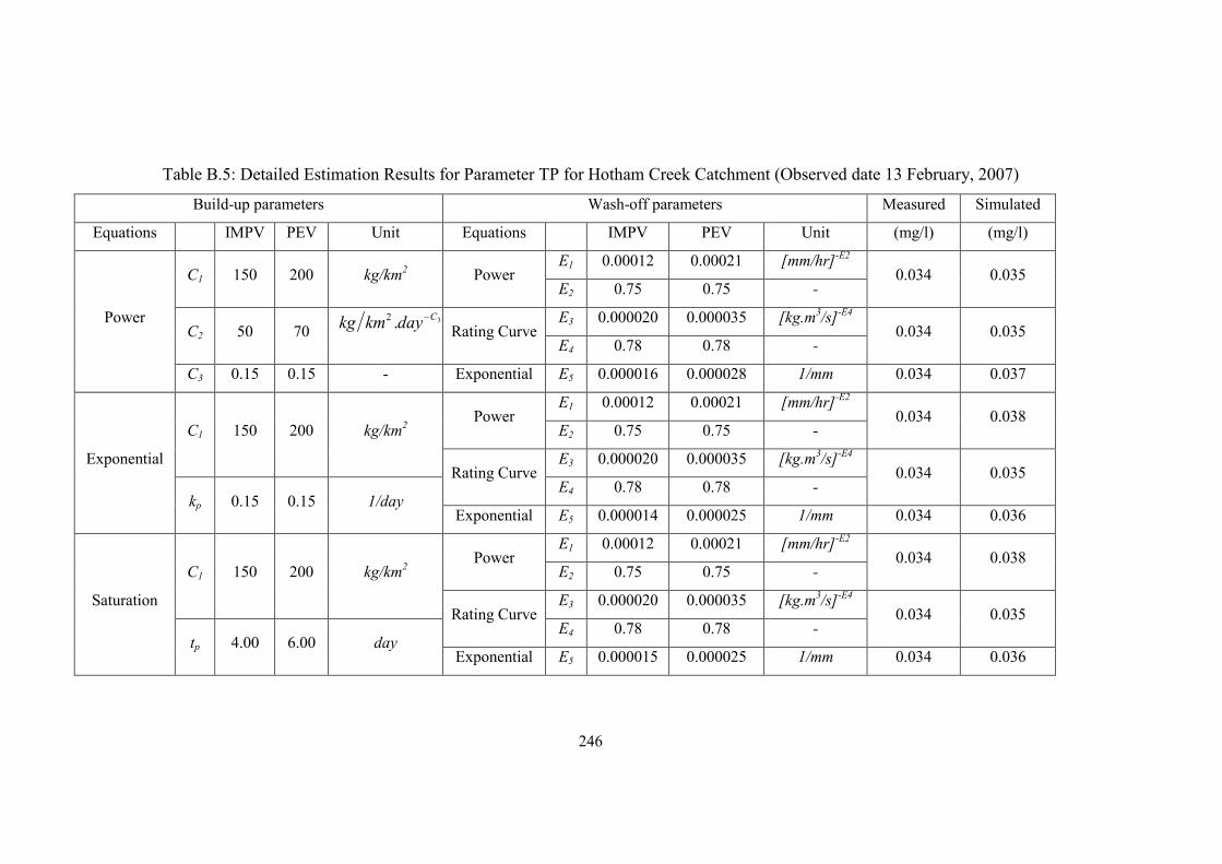
246

Table B.5: Detailed Estimation Results for Parameter TP for Hotham Creek Catchment (Observed date 13 February, 2007)



Power


0.034 0.035 E2 0.75 0.75 -

C2 50 70 3.2 Cdaykmkg −

Rating Curve

E3 0.000020 0.000035 [kg.m3/s]-E4

0.034 0.035 E4 0.78 0.78 -


Exponential


E1 0.00012 0.00021 [mm/hr]-E2 0.034 0.038

E2 0.75 0.75 -


0.034 0.035

kp 0.15 0.15 1/day E4 0.78 0.78 -

Exponential E5 0.000014 0.000025 1/mm 0.034 0.036

Saturation


E1 0.00012 0.00021 [mm/hr]-E2 0.034 0.038

E2 0.75 0.75 -


0.034 0.035

tp 4.00 6.00 day E4 0.78 0.78 -

Exponential E5 0.000015 0.000025 1/mm 0.034 0.036

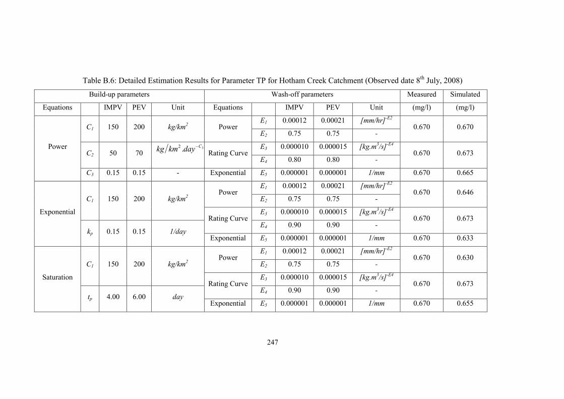
247

Table B.6: Detailed Estimation Results for Parameter TP for Hotham Creek Catchment (Observed date 8th July, 2008)



Power


0.670 0.670 E2 0.75 0.75 -

C2 50 70 3.2 Cdaykmkg −

Rating Curve

E3 0.000010 0.000015 [kg.m3/s]-E4

0.670 0.673 E4 0.80 0.80 -


Exponential


E1 0.00012 0.00021 [mm/hr]-E2 0.670 0.646

E2 0.75 0.75 -


0.670 0.673

kp 0.15 0.15 1/day E4 0.90 0.90 -

Exponential E5 0.000001 0.000001 1/mm 0.670 0.633

Saturation


E1 0.00012 0.00021 [mm/hr]-E2 0.670 0.630

E2 0.75 0.75 -


0.670 0.673

tp 4.00 6.00 day E4 0.90 0.90 -

Exponential E5 0.000001 0.000001 1/mm 0.670 0.655

248

Appendix C Build-up Wash-off Models Parameters for SWCC

249

Table C.1: Detailed Estimation Results for Parameter SS for Saltwater Creek Catchment (Observed date 6th December, 2004)



Power


20.00 18.228 E2 0.21 0.21 -

C2 2500 4500 3.2 Cdaykmkg −

Rating Curve

E3 0.180 0.330 [kg.m3/s]-E4

20.00 23.527 E4 0.30 0.30 -


Exponential

C1 6000 12000 kg/km2 Power

E1 0.030 0.050 [mm/hr]-E2 20.00 18.364

E2 0.21 0.21 -


20.00 23.527

kp 0.35 0.35 1/day E4 0.30 0.30 -

Exponential E5 0.00180 0.00340 1/mm 20.00 13.875

Saturation

C1 6000 12000 kg/km2 Power

E1 0.030 0.055 [mm/hr]-E2 20.00 16.114

E2 0.21 0.21 -


20.00 21.239

tp 1.50 2.00 day E4 0.30 0.30 -

Exponential E5 0.00180 0.00340 1/mm 20.00 12.045

250

Table C.2: Detailed Estimation Results for Parameter TN for Saltwater Creek Catchment (Observed date 6th December, 2004)



Power


0.950 0.996 E2 0.65 0.65 -

C2 200 350 3.2 Cdaykmkg −

Rating Curve

E3 0.0012 0.0020 [kg.m3/s]-E4

0.950 0.974 E4 0.84 0.84 -


Exponential


E1 0.0040 0.0065 [mm/hr]-E2 0.950 0.991

E2 0.65 0.65 -


0.950 0.974

kp 0.50 0.50 1/day E4 0.84 0.84 -

Exponential E5 0.00170 0.00280 1/mm 0.950 0.959

Saturation


E1 0.0050 0.0080 [mm/hr]-E2 0.950 0.964

E2 0.65 0.65 -


0.950 0.974

tp 1.50 2.00 day E4 0.84 0.84 -

Exponential E5 0.00170 0.00280 1/mm 0.950 0.817

251

Table C.3: Detailed Estimation Results for Parameter TN for Saltwater Creek Catchment (Observed date 3rd May, 2005)



Power


1.20 1.171 E2 0.80 0.80 -

C2 200 350 3.2 Cdaykmkg −

Rating Curve

E3 0.0012 0.0020 [kg.m3/s]-E4

1.20 1.187 E4 0.90 0.90 -


Exponential


E1 0.0050 0.0080 [mm/hr]-E2 1.20 1.275

E2 0.80 0.80 -


1.20 1.187

kp 0.50 0.50 1/day E4 0.90 0.90 -

Exponential E5 0.0020 0.0035 1/mm 1.20 0.985

Saturation


E1 0.0050 0.0080 [mm/hr]-E2 1.20 1.016

E2 0.80 0.80 -


1.20 1.187

tp 1.50 2.00 day E4 0.90 0.90 -

Exponential E5 0.0020 0.0035 1/mm 1.20 0.786

252

Table C.4: Detailed Estimation Results for Parameter TP for Saltwater Creek Catchment (Observed date 6th December, 2004)



Power


0.033 0.035 E2 0.75 0.75 -

C2 90 140 3.2 Cdaykmkg −

Rating Curve

E3 0.00010 0.00015 [kg.m3/s]-E4

0.033 0.046 E4 0.70 0.70 -


Exponential


E1 0.0003 0.0005 [mm/hr]-E2 0.033 0.045

E2 0.75 0.75 -


0.033 0.046

kp 0.10 0.10 1/day E4 0.70 0.70 -

Exponential E5 0.00013 0.00020 1/mm 0.033 0.045

Saturation


E1 0.0003 0.0005 [mm/hr]-E2 0.033 0.045

E2 0.75 0.75 -


0.033 0.046

tp 4.00 6.00 day E4 0.70 0.70 -

Exponential E5 0.00013 0.00020 1/mm 0.033 0.045

253

Table C.5: Detailed Estimation Results for Parameter TP for Saltwater Creek Catchment (Observed date 3rd May, 2005)



Power


0.120 0.115 E2 0.90 0.90 -

C2 90 140 3.2 Cdaykmkg −

Rating Curve

E3 0.00016 0.00028 [kg.m3/s]-E4

0.120 0.106 E4 0.78 0.78 -


Exponential


E1 0.0004 0.0007 [mm/hr]-E2 0.120 0.102

E2 0.90 0.90 -


0.120 0.114

kp 0.10 0.10 1/day E4 0.80 0.80 -

Exponential E5 0.00030 0.00050 1/mm 0.120 0.103

Saturation


E1 0.0004 0.0007 [mm/hr]-E2 0.120 0.119

E2 0.90 0.90 -


0.120 0.114

tp 4.00 6.00 day E4 0.80 0.80 -

Exponential E5 0.00030 0.00050 1/mm 0.120 0.121

254

Publications from this Thesis

Refereed Journal Papers

Hossain, I., Imteaz, M.A., Hossain, M.I. and Arulrajah, A. (Accepted).

Continuous simulation of suspended sediment through a stream section.

International Journal of Water.

Imteaz, M.A., Hossain, I. and Hossain, M.I. (Accepted). Estimation of build-up

and wash-off models parameters for an East-Australian catchment. International

Journal of Water.

Hossain, I., Imteaz, M.A. and Hossain, M.I. (Accepted) Application of a

catchment water quality model for an East-Australian catchment. International

Journal of Global Environmental Issues.

Hossain, I., Imteaz, M.A. and Hossain, M.I. (2011) Application of build-up and

wash-off models for an East-Australian catchment. World Academy of Science,

Engineering and Technology, 75(162): pp. 942 - 947.

Hossain, I., Imteaz, M.A., Gato-Trinidad, S. and Shanableh, A. (2010).

Development of a catchment water quality model for continuous simulations of

pollutants build-up and wash-off. International Journal of Civil and

Environmental Engineering, 2(4): pp. 210 - 217.

Refereed National and International Conference Papers

Hossain, I. and Imteaz, M.A. (2011). Continuous simulation of suspended

sediment transport along a stream section. Proceedings of the 34th IAHR World

Congress, Brisbane, Australia, 26th June to 1st July.

Hossain, I., Imteaz, M.A. and Hossain, M.I. (2010). Calibration of a catchment

water quality model for continuous simulations of SS, TN and TP. Proceedings

of the International Conference on Environment 2010, Batu Feringgi, Penang,

Malaysia, 13th – 15th December.

255

Hossain, I. and Imteaz, M.A. (2009). Development of a deterministic catchment

water quality model. Proceedings of the 32nd Hydrology and Water Resources

Symposium (H2009), Newcastle, New South Wales, Australia, 30th November –

3rd December.

Hossain, I. and Imteaz, M.A. (2009). Catchment water quality model:

Sensitivity analysis and parameters estimation. 3rd European Water and

Wastewater Management Conference, Birmingham, 22nd to 23rd September.

Development of an Integrated Catchment-Stream Water ...€¦ · For calibration and validation of...

Documents

Transcript of Development of an Integrated Catchment-Stream Water ...€¦ · For calibration and validation of...