
Development of an EEG cap allowing multichannel somato ... · either median or tibial nerve...
132
University of Fribourg Faculty of Science Department of Biology Development of an EEG cap allowing multichannel somato- sensory evoked potential recordings in macaque monkey Master thesis Anne-Dominique Gindrat Work conducted in the laboratory of Prof Eric M. Rouiller Under the supervision of Prof Eric M. Rouiller Department of Medicine Unit of Physiology January 2010
Transcript of Development of an EEG cap allowing multichannel somato ... · either median or tibial nerve...
University of Fribourg
Faculty of Science
Department of Biology
Development of an EEG cap allowing multichannel somato-
sensory evoked potential recordings in macaque monkey
Master thesis
Anne-Dominique Gindrat
Work conducted in the laboratory of Prof Eric M. Rouiller
Under the supervision of Prof Eric M. Rouiller
Department of Medicine
Unit of Physiology
January 2010
Remerciements Anne-Dominique Gindrat
Remerciements
Je voudrais pour commencer exprimer ma gratitude au Professeur Eric M. Rouiller qui
me donne la chance de faire mes études dans son laboratoire. Je lui suis très reconnais-
sante d’avoir supervisé et corrigé mon travail de Master, d’avoir consacré du temps pour ré-
pondre à mes questions et me donner des conseils.
Je tiens également à remercier chaleureusement le Dr Charles Quairiaux et le Dr Ju-
liane Britz, de l’université de Genève (Functional Brain Mapping Laboratory), qui tous deux
m’ont initiée à l’enregistrement et à l’analyse des potentiels évoqués somatosensoriels. Mer-
ci pour tout le temps qu’ils m’ont consacré ! Merci aussi à tous les membres de leur labora-
toire pour leur accueil et leur gentillesse, en particulier le Prof. Christoph Michel, Denis Bru-
net, le concepteur du programme Cartool, et le Dr Laurent Spinelli pour sa contribution à
l’élaboration du modèle 3D de notre bonnet d’électrodes.
Mes sincères remerciements vont bien sûr également à Florian Lanz pour sa précieuse
aide pendant les enregistrements, son ingéniosité, son aide pour l’élaboration du premier
modèle 3D du bonnet, l’entraînement du singe et sa bonne humeur !
Merci également à Mélanie Kaeser et Adjia Hamadjida qui m’ont apporté leur aide pour
l’acquisition et l’analyse des données comportementales.
Je souhaite aussi remercier Laurent Monnet, Véronique Moret et le Dr Thierry Wannier
pour leur contribution informatique plus que nécessaire !
Merci aussi à Josef Corpataux, Laurent Bossy, Bernard Aebischer et André Gaillard.
Pour conclure, je remercie toute l’équipe du laboratoire pour son accueil, son aide et sa
disponibilité, ainsi que toutes les personnes ayant participé de quelque manière que ce soit à
l’élaboration de ce travail.
Table of contents Anne-Dominique Gindrat
Table of contents I. Abstract ........................................................................................ 1 II. Introduction .................................................................................. 2
II.1. Monitoring of cerebral activity .......................................................................... 3 II.2. Neurophysiological basis of the electroencephalogram .................................. 5 II.3. Evoked potentials (EPs) ................................................................................ 11
II.3.1. History ............................................................................................................12 II.3.2. Somatosensory evoked potentials (SSEPs) ..................................................14 II.3.3. Somatosensory pathways from the skin to the cerebral cortex ......................15 II.3.4. Technique of SSEP recording in human ........................................................22 II.3.5. SSEP components .........................................................................................26 II.3.6. Cortical SSEP generators ..............................................................................29 II.3.7. Similarities between human and monkey SSEPs ..........................................30 II.3.8. Clinical applications .......................................................................................31 II.3.9. Factors altering the evoked responses ..........................................................35
II.4. Goals of the present study ............................................................................ 39 III. Material and methods ................................................................ 41
III.1. SSEP acquisition and analysis ...................................................................... 41 III.1.1. Anaesthesia and procedure ...........................................................................41 III.1.2. Peripheral nerve stimulation ..........................................................................43 III.1.3. Scalp SSEP recording ...................................................................................44 III.1.4. Data analysis .................................................................................................46 III.1.5. Scalp SSEP maps ..........................................................................................49 III.1.6. Identification of SSEP maps by cluster analysis ............................................50
III.2. Behavioural tests ........................................................................................... 51 IV. Results ........................................................................................ 54
IV.1. SSEP data .............................................................................................. 54 IV.1.1. Example of a typical SSEP recording ............................................................54 IV.1.2. Reproducibility of the recordings ....................................................................57 IV.1.3. Selection of the stimulation frequency ...........................................................69 IV.1.4. Selection of the stimulation intensity ..............................................................74 IV.1.5. Selection of the anaesthetic ...........................................................................77 IV.1.6. Scalp SSEPs after median nerve stimulation ................................................84 IV.1.7. Scalp SSEPs after tibial nerve stimulation .....................................................88
IV.2. Behavioural data .................................................................................... 91 IV.2.1. Modified Brinkman board task .......................................................................91 IV.2.2. Reach and grasp drawer task ........................................................................94
V. Discussion ................................................................................ 100
V.1. SSEP data ................................................................................................... 100 V.1.1. Stability of the SSEPs ..................................................................................100 V.1.2. Factors influencing the SSEPs.....................................................................102 V.1.3. Interpretation of scalp SSEP maps ..............................................................104
Table of contents Anne-Dominique Gindrat
V.1.4. Comparison with human data ......................................................................108 V.1.5. Protocol refinement ......................................................................................110 V.1.6. Advantages of multichannel SSEP recordings over previous techniques ....112
V.2. Behavioural data ......................................................................................... 113 V.3. Prospects .................................................................................................... 115
VI. Conclusion ............................................................................... 117 VII. References ................................................................................ 118 VIII. Appendixes ............................................................................... 126 Abbreviations
BAEP brain auditory evoked potentials
D Domitor®
e electrode
EEG electroencephalogram
EMG electromyogram
EP evoked potential
fMRI functional magnetic resonance imaging
GFP global field power
K Ketasol-100®
LSI laser speckle imaging
M1 primary motor cortex
MEP motor evoked potential
MRI magnetic resonance imaging
PET positron emission tomography
S1 primary somatosensory cortex
S2 secondary somatosensory cortex
SEM standard error of the mean
SPECT single-photon emission computerised tomography
SSEP somatosensory evoked potential
Abstract Anne-Dominique Gindrat
I. Abstract In this work, we present a simple and minimally invasive method to record somatosensory evoked
potentials (SSEPs) in an anaesthetized adult macaque monkey. The goal was to refine the epidural SSEP recording protocol previously used in the laboratory (Kaeser et al., 2006, 2007).
A customized electroencephalogram (EEG) cap containing 32 electrodes regularly distributed at the scalp was developed to perform scalp SSEP recordings. Electrical stimulations were delivered sepa-rately either to the median nerve at the wrist or to the tibial nerve at the ankle successively on each side, while the monkey was anaesthetized. The following parameters were tested: the stimulation frequency, the stimulation intensity, the type and dosage of anaesthesia. The SSEP data were analysed both conven-tionally in terms of component amplitude and latency at selected scalp locations and topographically by cluster analysis of the voltage maps. This topographical analysis is a data-driven approach and reveals a series of scalp topographies reflecting the steps in information processing.
The best responses were obtained with the following parameters: 0.5Hz frequency (1 sweep every 2 seconds) and slightly supra-liminar intensity electrical stimulation, 2.5% sevoflurane anaesthesia. Un-der these conditions, recordings appeared highly stable within the same session in terms of component amplitude and latency as well as regarding the topography of the SSEP maps. As expected, responses were somewhat less stable across the different sessions with respect to the amplitude and latency. How-ever, they were topographically highly reproducible. The map topography of the responses obtained after either median or tibial nerve stimulations was in line with the somatotopical organization of the sensori-motor cortex. In parallel, behavioural tests were conducted (modified Brinkman board task, reach and grasp drawer task).
The data presented here show that SSEPs can be successfully and reproducibly recorded from a multichannel EEG cap in the macaque monkey. This non-invasive method to record large-scale neuronal networks in real-time can be useful if repeated assessment of the cortical activity is desired, for example to study functional damage and recovery after a central nervous system lesion. In this case, topography of SSEPs will allow to assess the possible cortical reorganization of neuronal networks and relate it to functional recovery. The tool we developed is very relevant in the context of promoting non-invasive ap-proaches also in animal research.
1
Introduction Anne-Dominique Gindrat
II. Introduction Understanding the functioning of the brain is since ancient time a recurrent con-
cern. In particular, what happens in the brain following a lesion in the central nervous
system? To answer such a question, it has been necessary to develop methods to
explore the brain, especially approaches to evaluate the extent of a lesion in vivo, be-
fore the histological study. This assessment can be invasive, as in the case of laser
speckle imaging (LSI), or non-invasive, using for example the electroencephalogram
(EEG), the evoked potential (EP) method or the magnetic resonance imaging (MRI).
Given that the human brain can not always be directly investigated, animal models
are used as substitution. In neurophysiology, a prime model is the monkey because
the organisation of its nervous system is very similar to that of human.
The purpose of this Master thesis was to develop an EEG cap and to adjust all
the recording parameters, allowing multichannel somatosensory evoked potential
(SSEP) recording in macaque monkeys. Such recordings at the whole scalp have
only rarely been performed in monkeys until now (Fontanarosa et al., 2004). In these
animals, SSEP recordings were performed predominantly in an invasive way, namely
on the surface of the meninges or into the cortex (Allison et al., 1991a, 1991b;
Arezzo et al., 1979, 1981; Kaeser et al., 2006, 2007; McCarthy et al., 1991). The goal
was to address the general feasibility of the technique and then to obtain stable and
reproducible SSEP recordings in order to use this method in longer term for the
monitoring of the cerebral activity before and after a lesion that may be spinal, corti-
cal or subcortical, as in the case of models in monkeys for spinal cord injury, stroke
or Parkinson disease. In these three cases, the cortical map very likely undergoes
changes following the lesion. Consequently, SSEP recording using an EEG cap may
be a good alternative to previous methods, such as intracortical microstimulation, to
evaluate this cortical reorganization thanks to its minimally invasive nature. SSEPs
may also be a good predictor of the outcome after the brain lesion, as reported in
previous studies in human (Carter and Butt, 2001, 2005; Carter et al., 1999).
2
Introduction Anne-Dominique Gindrat
II.1. Monitoring of cerebral activity
For a very long time, human has been being fascinated by the brain. In the pre-
historic age already, some brain operations (trepanations) on humans were carried
out (Bear et al., 2006). Moreover, the frequent neurological disorders have encour-
aged researchers to develop new methods to investigate the brain. At the moment,
our knowledge of the brain keeps progressing and new techniques are developed in
order to attempt to penetrate the numerous mysteries it still contains. A good illustra-
tion of this is the development of methods used to monitor the brain activity. They are
not only relevant to detect neurological disorders, but also to study the normal func-
tions of the brain for research purposes. To this aim, animal models are required
given that some of these procedures are invasive. In this section, a brief skimming
over some current brain monitoring methods in human and in animal will be per-
formed.
Neurological monitoring methods in human and animal can be based on the de-
tection of intracranial pressure, blood flow dynamics or on the recording of the elec-
trical activity of the brain (Mani and Absalom, 2006; Umamaheswara Rao, 2002).
Methods for imaging the functional activity of the brain, such as the functional
magnetic resonance imaging (fMRI), the positron emission tomography (PET) or the single-photon emission computerised tomography (SPECT), detect the haemody-
namic response, and hence metabolism changes, resulting from the brain activity.
fMRI, PET and SPECT are largely used in human (see for example Jacobs et al.,
2003; Tatsch et Ell, 2006; Tibbo et al., 1997; Weiler et al., 2006) and animal (see for
example Avery et al., 2000; Blaizot et al., 2000; Stefanacci et al., 1998) due to their
non-invasiveness. However, the major disadvantage is that they have a poor tempo-
ral resolution which can not resolve the fast neuronal activity (Bear et al., 2006; Kan-
del et al., 2000; Purves et al., 2004).
Another method, called magnetoencephalography (MEG), allows the non-
invasive investigation of the brain. MEG detects at the scalp the small amplitude
magnetic forces generated by the electrical activity of the brain neurons. A great ad-
3
Introduction Anne-Dominique Gindrat
vantage of this procedure is its high spatial and temporal resolution. However, this
technique is still in development and its applications are not well defined. Moreover,
its high cost and low availability represent major limitations (Panayiotopouls, 2005).
Moreover, in animals such as monkeys or cats, intracortical microstimulation
(ICMS) can be performed, mainly to study motor outputs. This electrophysiological
procedure is based on the same principle as the one developed in the 1930s by Pen-
field to build somatotopic maps. That is to say, a microelectrode is inserted at differ-
ent sites and different depths into the cortex and current is applied. This electrical
stimulation triggers primarily responses of the contralateral side of the body. It is
therefore possible to map the somatotopic organisation of the motor cortex and to
evaluate some potential cortical reorganization following a cortical lesion. This
method has been previously described in more detail by Asanuma and Rosén
(1972), Sessle and Wiesendanger (1982), Liu and Rouiller (1999), Rouiller et al.
(1998), Schmidlin et al. (2004, 2005) and Wyss (2007). It is also possible to perform
local electrophysiological recordings with chronically implanted electrodes (Buzsáki,
2004).
Another method has been developed in animals such as monkeys or rats, and
in human, namely the LSI (Dunn et al., 2001; Durduran et al., 2004; Weber et al.,
2004; Zhou et al., 2008) or Laser Speckle Contrast Analysis (LASCA) (Hecht et al.,
2009). This optical functional imaging technique allows to study with very high resolu-
tion the spatiotemporal dynamics of the cerebral blood flow on the surface of the cor-
tex and therefore indirectly assesses possible changes in the brain activity if a lesion
is performed. The underlying principle of LSI is a laser beam being differently re-
flected by the cortical surface depending on the blood flow.
Both of these latter methods offer a high spatial and temporal resolution. Never-
theless, they are invasive, what constitutes a major limitation. Indeed, it restricts the
possibility to investigate the brain of the same animal in a repeated manner. Equally
important, they allow investigating only a restricted brain area. As a consequence,
scalp recordings of the brain electrical activity are performed given that they are
minimally invasive and powerful to drive the cortical activity in the whole brain. Two
4
Introduction Anne-Dominique Gindrat
valuable electrophysiological methods, namely the EEG and the EPs, are available.
The main advantage of both these approaches is their good temporal resolution (in
the order of ms) allowing to follow the different steps of information processing in the
brain with precision. On the other hand, their spatial resolution is low.
The EEG allows recording the spontaneous brain potentials generated by a
large population of neurons using electrodes placed at the scalp. Consequently, this
technique is non-invasive, safe and painless. Moreover, it enables to monitor the ac-
tivity of the whole brain, what is a great advantage. The EEG signals depend on the
activity state of the subject’s brain: when the subject is awake or in the paradoxal
sleep, the EEG is primarily composed of high frequency and low amplitude signals.
On the contrary, in the profound sleep, the EEG frequency is low and the amplitude
high. EEG can also be directly recorded on the meninges surface and are called in
this case electrocorticography (ECoG)1.The SSEP recording is another powerful non-
invasive method to investigate the whole brain activity. This last technique, which re-
cords the brain activity generated after a stimulus, will be discussed in detail in the
following sections.
II.2. Neurophysiological basis of the electroencephalogram
The EEG is a method allowing recording the electrical activity at the scalp gen-
erated by neurons into the brain. The morphology or the generator structures will be
exposed briefly. Then the basic processes underlying the EEG will be described:
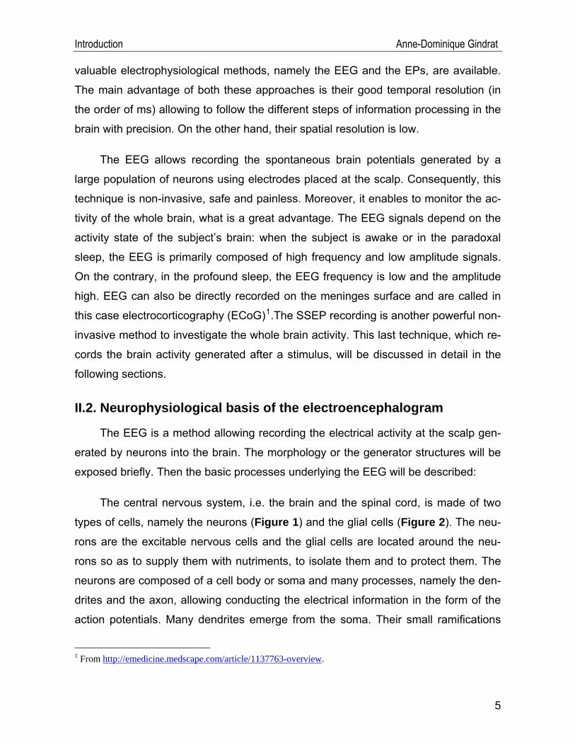
The central nervous system, i.e. the brain and the spinal cord, is made of two
types of cells, namely the neurons (Figure 1) and the glial cells (Figure 2). The neu-
rons are the excitable nervous cells and the glial cells are located around the neu-
rons so as to supply them with nutriments, to isolate them and to protect them. The
neurons are composed of a cell body or soma and many processes, namely the den-
drites and the axon, allowing conducting the electrical information in the form of the
action potentials. Many dendrites emerge from the soma. Their small ramifications
1 From http://emedicine.medscape.com/article/1137763-overview.
5
Introduction Anne-Dominique Gindrat
enable the neuron to collect the electrical potential from other neurons and to con-
duct it to the axon hillock in order to potentially generate an action potential. The
axon is the process which conducts very rapidly the action potential generated in the
axon hillock to other neurons via the synapses. These latter structures are junctions
generally between axons and dendrites which allow conducting the electrical informa-
tion from a neuron to another one. This transport of electrical information is made
possible via the neurotransmitters (for further details, see Bear et al., 2006, p 23-48).
Figure 1 : Schematic structure of a pyramidal neuron. The cell body or soma is surrounded by two types of processes: the dendrites are the main input structures, receiving the information from other neurons and transporting it to the soma. Note however that the soma is also an input zone. The axon is the output structure which conducts the in-formation to other neurons via synapses. The axon is wrapped by a myelin sheet, isolating it and thus allowing increasing the transmission speed of the action potential. This isolating sheet is not continuous but there are some gaps called nodes of Ranvier. They allow increasing the transmission speed by saltatory conduction. The axon is linked to the soma through the axon hillock which is the region generating the action potentials. The axon can split in several axon collaterals whose end then divides in ter-minal buttons forming actually the synaptic region. All these structures allow the neuron to process the informa-tion and to transmit it to other neurons (from Kandel et al., 2000, p.22).
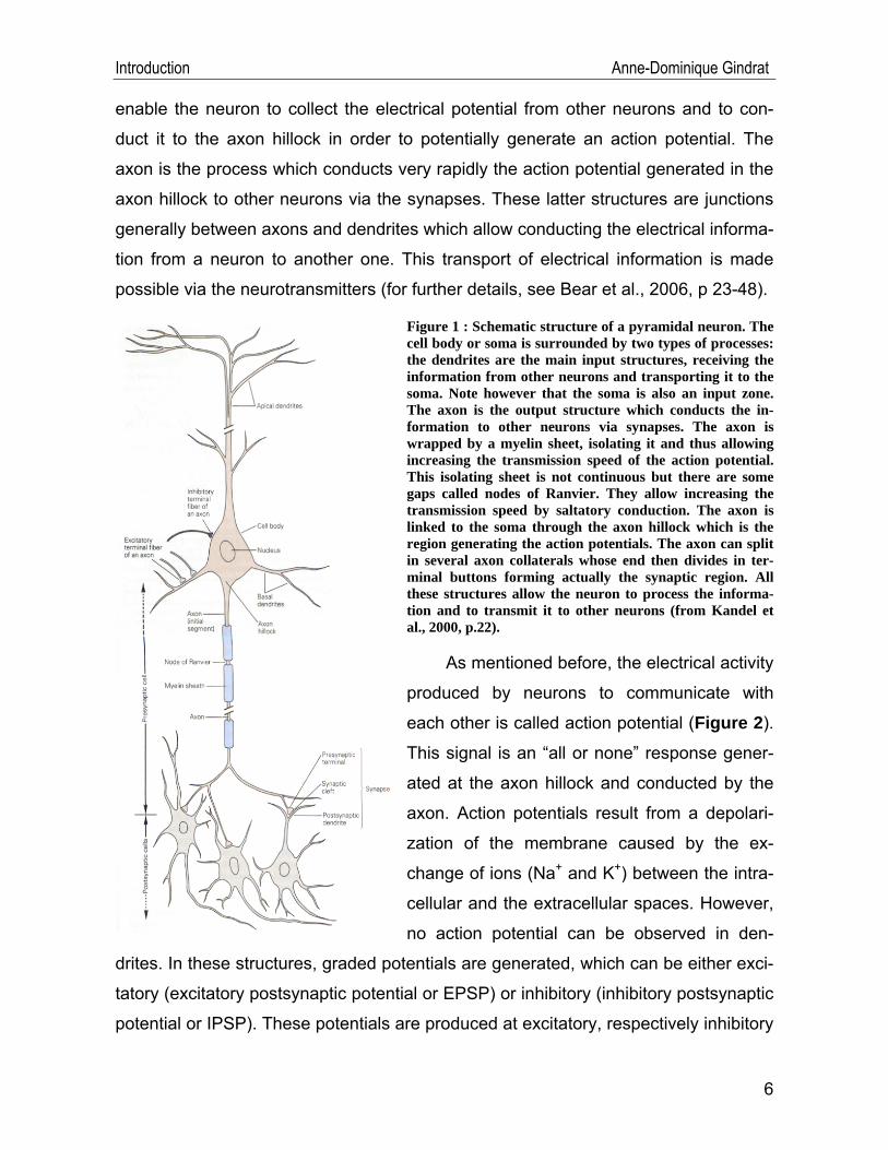
As mentioned before, the electrical activity
produced by neurons to communicate with
each other is called action potential (Figure 2).
This signal is an “all or none” response gener-
ated at the axon hillock and conducted by the
axon. Action potentials result from a depolari-
zation of the membrane caused by the ex-
change of ions (Na+ and K+) between the intra-
cellular and the extracellular spaces. However,
no action potential can be observed in den-
drites. In these structures, graded potentials are generated, which can be either exci-
tatory (excitatory postsynaptic potential or EPSP) or inhibitory (inhibitory postsynaptic
potential or IPSP). These potentials are produced at excitatory, respectively inhibitory
6
Introduction Anne-Dominique Gindrat
synapses by the release of neurotransmitters. Such potentials coming from many
dendrites converge passively to the soma where they are then spatially and tempo-
rally summated. If a membrane threshold is reached (about -65mV), an action poten-
tial is generated at the axon hillock and propagates actively along the axon. It is ad-
mitted that the EPSP and IPSP are of paramount signification in the generation of the
EEG signals (Speckmann and Elger, 1987). Therefore, these processes will be dis-
cussed in more detail below.
Figure 2 : Overall view of the interaction between neurons and glial cells. Two types of glial cells are rep-resented in this figure: the astrocytes, which establish the connections between neurons and blood vessels, and the oligodendrocytes that wrap the axon, making the myelin sheet in the central nervous system (in the peripheral nervous system, the myelin sheet is provided by the Schwann cells). In the upper right-hand corner, a synapse between two neurons is depicted: an action potential arrives at the axon terminal of the presynaptic neuron, what triggers the release of neurotransmitter containing synaptic vesicles in the synaptic cleft. The neurotransmitters molecules bind then to receptors on the dendrites of postsynaptic neurons, triggering the formation of a postsynaptic potential (from http://pubpages.unh.edu/~jel/images/brain_glia.jpg).
The generation of an EPSP results in a net inflow of cations across the sub-
synaptic membrane causing a depolarization. This is due to a potential gradient de-
veloping along the subsynaptic neuronal membrane in the intra- and extracellular
space in response to an excitatory synapse activated by an action potential in the
presynaptic neuron. The result of this gradient is a movement of cations along the
nerve cell membrane from the extracellular space toward the subsynaptic region. An
inverted flow of cations is observed in the intracellular space. On the other hand, in
response to an activated inhibitory synapse, the onset of an IPSP coincides with a
7
Introduction Anne-Dominique Gindrat
net outflow of cations from the intra- to the extracellular space which can go with an
inflow of anions into the intracellular space, increasing first the membrane potential at
the subsynaptic membrane in comparison with the surrounding regions. A potential
gradient is therefore generated along the membrane. This results in a flow of cations
in the extracellular space from the subsynaptic membrane to the surrounding re-
gions. An inverted flow is measured in the intracellular medium. These ions move-
ments in the extracellular space are the basis of the generation of the EEG signals
(Speckmann and Elger, 1987). They produce the so-called extracellular field poten-
tials (Speckmann and Elger, 1987).
Nevertheless, Speckmann and Elger (1987) specified that glial cells can also
contribute to the generation of extracellular potentials producing the EEG signals
given that the membrane potential of these cells depends largely on the extracellular
potassium concentration. A potential gradient along the membrane of glial cells and
subsequent intra- and extracellular current flows can build up, in the same way as
those previously described following a postsynaptic potential. Moreover, these cells
have long processes connecting them each other, allowing the potential fields to
spread. Therefore, glial cells can amplify the extracellular field potentials.
The synaptic processes generating the field potentials, in other words the con-
tribution of each individual neuron to the EEG, will be now outlined in greater detail.
To this aim, Figure 3 and Figure 4 will be considered. These processes have been
described in Kandel et al. (2000) and Speckmann and Elger (1987). The EEG signal
results primarily from the activity of pyramidal cells (Figure 1) which represent the
main projection neurons in the cerebral cortex. Many synapses are formed with the
dendrites of these cells, oriented perpendicularly to the cortical surface. The EEG
signals result primarily from such synaptic activity in these pyramidal cells.
Let’s consider first the activation of an excitatory synapse (EPSP) on the apical den-
drite of a pyramidal neuron, in layers 2 and 3, by a contralateral cortical afferent axon
(Figure 3 and Figure 4B). This causes, as mentioned previously, an inward flow of
cations into the dendrite at the synaptic site where the EPSP is generated, resulting
in the formation of a current sink. This current flows then down the dendrite and
8
Introduction Anne-Dominique Gindrat
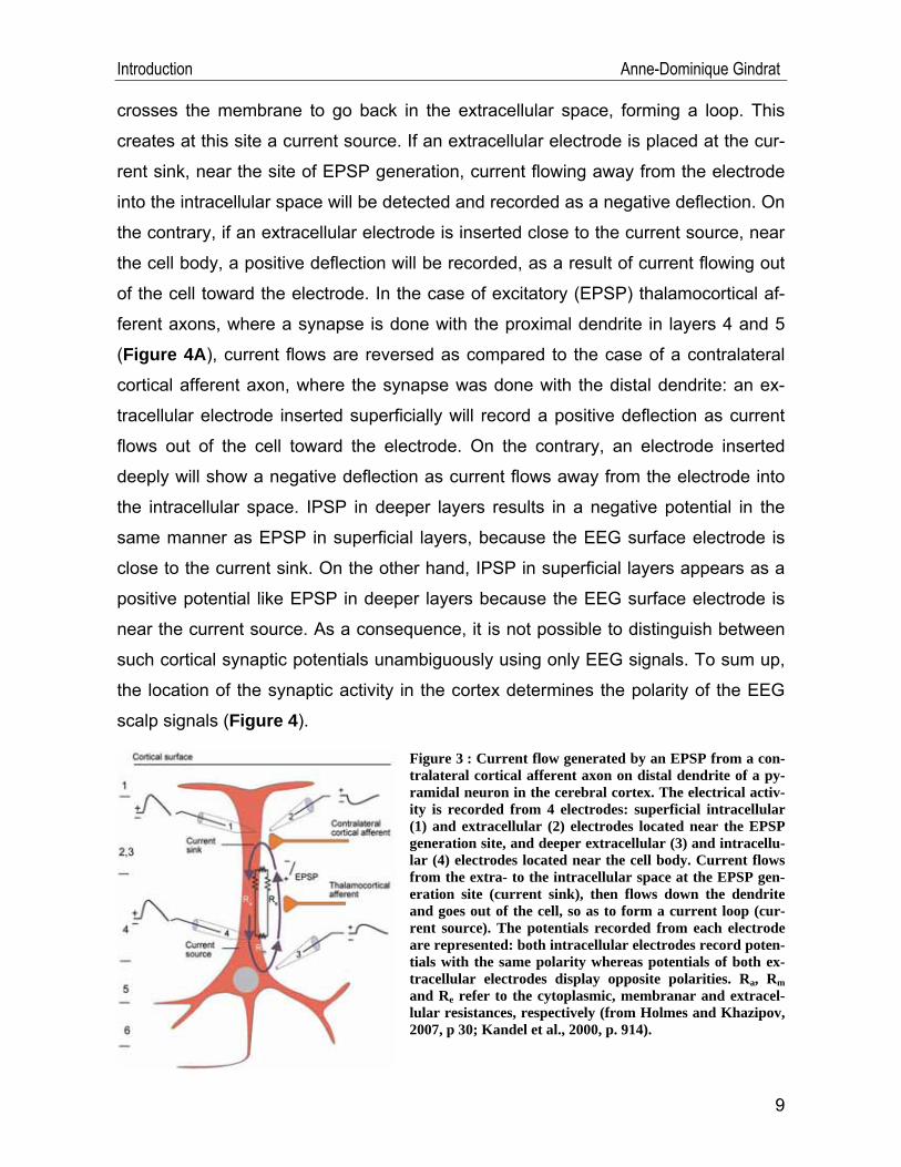
crosses the membrane to go back in the extracellular space, forming a loop. This
creates at this site a current source. If an extracellular electrode is placed at the cur-
rent sink, near the site of EPSP generation, current flowing away from the electrode
into the intracellular space will be detected and recorded as a negative deflection. On
the contrary, if an extracellular electrode is inserted close to the current source, near
the cell body, a positive deflection will be recorded, as a result of current flowing out
of the cell toward the electrode. In the case of excitatory (EPSP) thalamocortical af-
ferent axons, where a synapse is done with the proximal dendrite in layers 4 and 5
(Figure 4A), current flows are reversed as compared to the case of a contralateral
cortical afferent axon, where the synapse was done with the distal dendrite: an ex-
tracellular electrode inserted superficially will record a positive deflection as current
flows out of the cell toward the electrode. On the contrary, an electrode inserted
deeply will show a negative deflection as current flows away from the electrode into
the intracellular space. IPSP in deeper layers results in a negative potential in the
same manner as EPSP in superficial layers, because the EEG surface electrode is
close to the current sink. On the other hand, IPSP in superficial layers appears as a
positive potential like EPSP in deeper layers because the EEG surface electrode is
near the current source. As a consequence, it is not possible to distinguish between
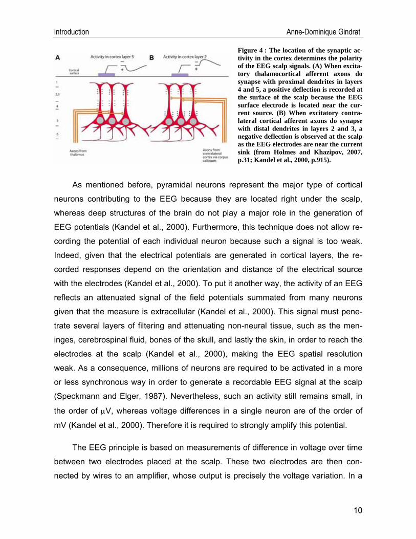
such cortical synaptic potentials unambiguously using only EEG signals. To sum up,
the location of the synaptic activity in the cortex determines the polarity of the EEG
scalp signals (Figure 4).
9
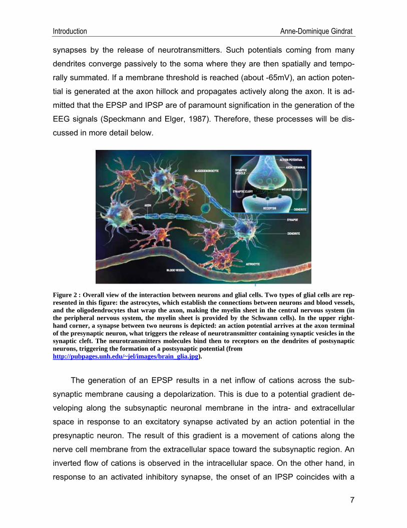
914).
Figure 3 : Current flow generated by an EPSP from a con-tralateral cortical afferent axon on distal dendrite of a py-ramidal neuron in the cerebral cortex. The electrical activ-ity is recorded from 4 electrodes: superficial intracellular (1) and extracellular (2) electrodes located near the EPSP generation site, and deeper extracellular (3) and intracellu-lar (4) electrodes located near the cell body. Current flows from the extra- to the intracellular space at the EPSP gen-eration site (current sink), then flows down the dendrite and goes out of the cell, so as to form a current loop (cur-rent source). The potentials recorded from each electrode are represented: both intracellular electrodes record poten-tials with the same polarity whereas potentials of both ex-tracellular electrodes display opposite polarities. Ra, Rm and Re refer to the cytoplasmic, membranar and extracel-lular resistances, respectively (from Holmes and Khazipov, 2007, p 30; Kandel et al., 2000, p.
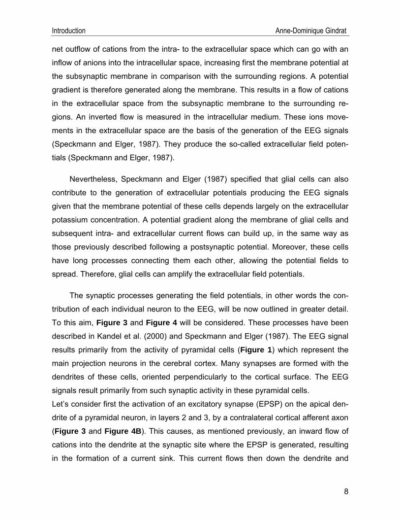
Introduction Anne-Dominique Gindrat
Figure 4 : The location of the synaptic ac-tivity in the cortex determines the polarity of the EEG scalp signals. (A) When excita-tory thalamocortical afferent axons do synapse with proximal dendrites in layers 4 and 5, a positive deflection is recorded at the surface of the scalp because the EEG surface electrode is located near the cur-rent source. (B) When excitatory contra-lateral cortical afferent axons do synapse with distal dendrites in layers 2 and 3, a negative deflection is observed at the scalp as the EEG electrodes are near the current sink (from Holmes and Khazipov, 2007, p.31; Kandel et al., 2000, p.915).
As mentioned before, pyramidal neurons represent the major type of cortical
neurons contributing to the EEG because they are located right under the scalp,
whereas deep structures of the brain do not play a major role in the generation of
EEG potentials (Kandel et al., 2000). Furthermore, this technique does not allow re-
cording the potential of each individual neuron because such a signal is too weak.
Indeed, given that the electrical potentials are generated in cortical layers, the re-
corded responses depend on the orientation and distance of the electrical source
with the electrodes (Kandel et al., 2000). To put it another way, the activity of an EEG
reflects an attenuated signal of the field potentials summated from many neurons
given that the measure is extracellular (Kandel et al., 2000). This signal must pene-
trate several layers of filtering and attenuating non-neural tissue, such as the men-
inges, cerebrospinal fluid, bones of the skull, and lastly the skin, in order to reach the
electrodes at the scalp (Kandel et al., 2000), making the EEG spatial resolution
weak. As a consequence, millions of neurons are required to be activated in a more
or less synchronous way in order to generate a recordable EEG signal at the scalp
(Speckmann and Elger, 1987). Nevertheless, such an activity still remains small, in
the order of μV, whereas voltage differences in a single neuron are of the order of
mV (Kandel et al., 2000). Therefore it is required to strongly amplify this potential.
The EEG principle is based on measurements of difference in voltage over time
between two electrodes placed at the scalp. These two electrodes are then con-
nected by wires to an amplifier, whose output is precisely the voltage variation. In a
10
Introduction Anne-Dominique Gindrat
normal EEG, the amplitude ranges as a rule from -100μV to +100μV and the fre-
quency generally from 0.5Hz and 45Hz in healthy subjects (δ waves: 0.5-3.5Hz; θ
waves: 4-7.5Hz; α waves: 8-13Hz; β waves: 14-30Hz; γ waves 31-45Hz) (Coles and
Rugg, 1996; Sanei and Chambers, 2007).
If a repeated stimulation is delivered during the EEG recording, voltage changes
can be observed, which are time-locked with the stimulation. Consequently, it is pos-
sible to determine an epoch, beginning some dozens of ms before the stimulus and
lasting for some hundreds of ms after the stimulus. The activity generated during this
period of time corresponds to responses of the nervous system to this stimulus.
These signals are called evoked potentials or event-related potentials. This last de-
nomination is due to the fact that these potentials are not just strictly evoked by the
stimulation, but can be “invoked by the psychological demand of the situation”, hence
the more neutral expression of event-related potentials (Coles and Rugg, 1996).
Nevertheless, in the present work, we will speak about evoked potentials.
II.3. Evoked potentials (EPs)
EPs are described as electrical signals appearing in a sensory receptor, a nerve
or a region of the central nervous system following a stimulation (Berthet, 2006) and
correspond to reception, transmission and processing of the stimulus (Freye, 2005).
Desmedt (1987) adds that EPs appear with «phasic changes of the potential fields
produced in the conductive volume of the head by a volley of afferent impulses». Ac-
cordingly, EPs differ from EEG or electromyogram (EMG) activity which refers to
spontaneous potentials.
Following a stimulation, the afferent sensory volley moves from the periphery to
the brain, and responses - extracellular potentials - are produced along this afferent
sensory pathway by successive anatomic neural generators. These potentials are the
result of the synchronous response (action potentials and synaptic potentials) of a
population of neurons activated by the stimulus (Aminoff and Eisen, 1998). However,
this signal is very low, in the order of 1-20μV, what is much lower than the EEG, ECG
or EMG activity (Freye, 2005; Mauguière and Fischer, 1990). Moreover, other electri-
11
Introduction Anne-Dominique Gindrat
cal potentials resulting from the spontaneous nervous system activity (EEG) may mix
up with the response to the stimulation, generating undesirable noise. The goal is
therefore to improve the signal to noise ratio in order to obtain a clear response to the
stimulus. To this aim, signal averaging is required. To put it another way, responses
are added in such a way that those which appear in a synchronous way with the
stimulation are amplified. On the contrary, randomly generated potentials cancel
each other out because of their variable polarity (Desmedt, 1987; Mauguière and
Fischer, 1990). The remaining response corresponds to potentials evoked by the
stimulation. This technique was developed by Dawson in 1954. Nevertheless, it is
possible that rhythmic activity, such as cardiac activity, remains visible in the SSEP
recordings.
II.3.1. History
The first measurements of both spontaneous and evoked potentials were very
likely accomplished by Richard Caton (1842-1926), a doctor from Liverpool, from the
brains of animals using a galvanometer and two electrodes at the scalp (Caton,
1875; Cohen of Birkenhead, 1959; Haas, 2003; Ormerod, 2006, Sanei and Cham-
bers, 2007). These results were published in 1875. In 1924, Hans Berger, a German
neurologist, recorded the first spontaneous EEG activity from humans. From then on,
the term electro- (registration of brain electrical activities) encephalo- (emitting the
signals from the head) gram (drawing or writing) was proposed to describe the elec-
trical neural activity of the brain. The method of EPs allowed mapping of several cor-
tical areas in response to sensory stimulation in animals (Desmedt, 1987). For ex-
ample, Bremer and Dow (1939) located precisely the auditory cortex of the cat using
two cotton electrodes and “clicks” as auditory stimuli. Then, Adrian (1941) mapped
the “somatic receiving area” in several mammals, namely the somesthesic cortex,
using mechanical stimulations of skin and pressure receptors and by recording the
brain activity with electrodes placed on the surface of the cortex or with intracortical
electrodes. The method of EPs was also used by Marshall et al. (1941) to map the
somatosensory cortex in cats and monkeys, and these results will be presented far-
ther in section II.3.3. Subsequently, the technique of EP recording was applied to
human patients suffering from myoclonus (Dawson, 1947b) and to healthy humans
12
Introduction Anne-Dominique Gindrat
(Dawson, 1947a). One of the most important contributions in EP recording is due to
Georges Dawson who developed a method of photographic overtrace allowing sup-
pressing nonrelated potentials and to extract the signals evoked by the stimulation
(Desmedt, 1987; Erwin et al., 1987). This averaging device was afterward improved
by increasing the sampling rate so as to allow for the recording of high frequency
SSEP components (Erwin et al., 1987) and numerical averaging methods were de-
veloped (Desmedt, 1987).
However, at the outset, the relevance of EPs was not obvious as compared to
the EEG (Desmedt, 1987). Papers were indeed published to demonstrate that the
EEG was “entering a stage of usefulness” (Walter, 1937). On the other hand, the first
papers about EPs, such as Dawson’s ones (1947a; 1947b), only reported “potential
changes on the scalp” following an electrical stimulation of a peripheral nerve (Daw-
son, 1947s), but their clinical pertinence was not evident at that time. Nevertheless,
some authors, such as Adrian (1936), understood that EPs would be relevant to
measure the electrical activity of the brain. Indeed, he wrote:
“To give potential changes measurable through the skull in man a fairly large number of cortical neurons must work in unison. In normal activity with the eyes open there will be little opportunity for this, and we can only record the rapid, irregular oscillations which are the summed response of many independent groups. Rhythmical afferent stimulation may produce a corresponding cortical rhythm, and if a large enough area is affected the potential changes will be appreciable. Thus if the whole visual field is made to flicker, a corresponding potential rhythm can be detected in the occipital region.” (Adrian, 1936)
The importance of SSEPs in clinical use (see for example Carter and Butt,
2005; Desmedt, 1987; Feys et al., 2000; Giesser, 1993; Machado, 1996) was only
appreciated several years later with some developments of this method, such as the
improvement of differential amplifiers in parallel with the development of new transis-
tors and integrated circuitry, the reduction in size of the equipment allowing more ex-
tensive intraoperative use, the development of signal-averaging techniques to extract
small signals from electrical noise and the expansion of computerized equipment with
microprocessors allowing multiple channel recordings, filtering and spectral
13
Introduction Anne-Dominique Gindrat
sis2. Some of these clinical applications will be exposed later (section II.3.8).
II.3.2. Somatosensory evoked potentials (SSEPs)
ed stimulation:
), including the brain stem AEPs (BAEPs)
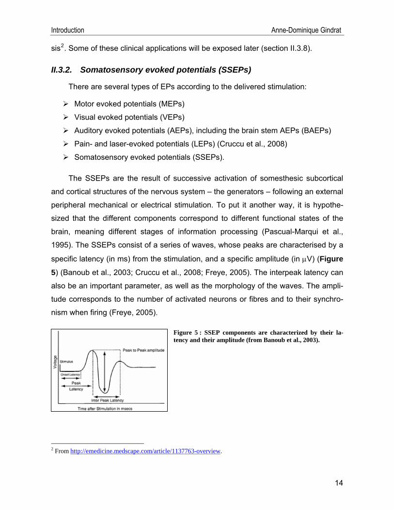
The SSEPs are the result of successive activation of somesthesic subcortical
Figure 5 : SSEP components are characterized by their la-tency and their amplitude (from Banoub et al., 2003).
There are several types of EPs according to the deliver
Motor evoked potentials (MEPs)
Visual evoked potentials (VEPs)
Auditory evoked potentials (AEPs
Pain- and laser-evoked potentials (LEPs) (Cruccu et al., 2008)
Somatosensory evoked potentials (SSEPs).
and cortical structures of the nervous system – the generators – following an external
peripheral mechanical or electrical stimulation. To put it another way, it is hypothe-
sized that the different components correspond to different functional states of the
brain, meaning different stages of information processing (Pascual-Marqui et al.,
1995). The SSEPs consist of a series of waves, whose peaks are characterised by a
specific latency (in ms) from the stimulation, and a specific amplitude (in μV) (Figure
5) (Banoub et al., 2003; Cruccu et al., 2008; Freye, 2005). The interpeak latency can
also be an important parameter, as well as the morphology of the waves. The ampli-
tude corresponds to the number of activated neurons or fibres and to their synchro-
nism when firing (Freye, 2005).
2 From http://emedicine.medscape.com/article/1137763-overview.
14
Introduction Anne-Dominique Gindrat
II.3.3. Somatosensory pathways from the skin to the cerebral cortex
The somatosensory system is able to distinguish between five different types of
bodily sensations, namely the discriminative touch or mechanoreception (perception
of size, shape, texture, movement of an object across the skin, as well as vibration
and pressure), the proprioception (perception of static position and movements of the
limbs and body mediated by the measurement of muscles stretch, tendon tension
and joint position), the nociception (sensation of pain or itching due to a chemical
agent or tissue damage), the temperature sense or thermoreception (distinction be-
tween warmth and cold) and the visceroception (perception of the physiological state
of internal organs, part of the autonomous nervous system) (Cruccu et al., 2008;
Kandel et al., 2000). These different sub-modalities are mediated by distinct periph-
eral receptors, spinal pathways and target areas in the brain. As a consequence, one
can differentiate between two major afferent pathways, each of them constituted of
three neurons.
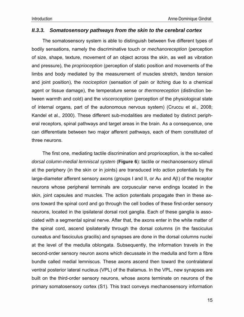
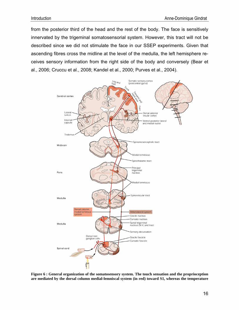
The first one, mediating tactile discrimination and proprioception, is the so-called
dorsal column-medial lemniscal system (Figure 6): tactile or mechanosensory stimuli
at the periphery (in the skin or in joints) are transduced into action potentials by the
large-diameter afferent sensory axons (groups I and II, or Aα and Aβ) of the receptor
neurons whose peripheral terminals are corpuscular nerve endings located in the
skin, joint capsules and muscles. The action potentials propagate then in these ax-
ons toward the spinal cord and go through the cell bodies of these first-order sensory
neurons, located in the ipsilateral dorsal root ganglia. Each of these ganglia is asso-
ciated with a segmental spinal nerve. After that, the axons enter in the white matter of
the spinal cord, ascend ipsilaterally through the dorsal columns (in the fasciculus
cuneatus and fasciculus gracilis) and synapses are done in the dorsal columns nuclei
at the level of the medulla oblongata. Subsequently, the information travels in the
second-order sensory neuron axons which decussate in the medulla and form a fibre
bundle called medial lemniscus. These axons ascend then toward the contralateral
ventral posterior lateral nucleus (VPL) of the thalamus. In the VPL, new synapses are
built on the third-order sensory neurons, whose axons terminate on neurons of the
primary somatosensory cortex (S1). This tract conveys mechanosensory information
15
Introduction Anne-Dominique Gindrat
from the posterior third of the head and the rest of the body. The face is sensitively
innervated by the trigeminal somatosensorial system. However, this tract will not be
described since we did not stimulate the face in our SSEP experiments. Given that
ascending fibres cross the midline at the level of the medulla, the left hemisphere re-
ceives sensory information from the right side of the body and conversely (Bear et
al., 2006; Cruccu et al., 2008; Kandel et al., 2000; Purves et al., 2004).
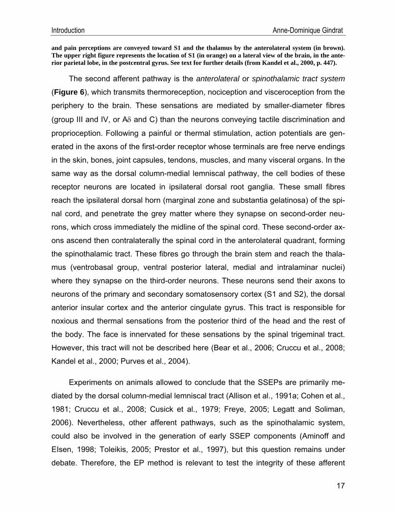
Figure 6 : General organization of the somatosensory system. The touch sensation and the proprioception are mediated by the dorsal column medial-lemniscal system (in red) toward S1, whereas the temperature
16
Introduction Anne-Dominique Gindrat
and pain perceptions are conveyed toward S1 and the thalamus by the anterolateral system (in brown). The upper right figure represents the location of S1 (in orange) on a lateral view of the brain, in the ante-rior parietal lobe, in the postcentral gyrus. See text for further details (from Kandel et al., 2000, p. 447).
The second afferent pathway is the anterolateral or spinothalamic tract system
(Figure 6), which transmits thermoreception, nociception and visceroception from the
periphery to the brain. These sensations are mediated by smaller-diameter fibres
(group III and IV, or Aδ and C) than the neurons conveying tactile discrimination and
proprioception. Following a painful or thermal stimulation, action potentials are gen-
erated in the axons of the first-order receptor whose terminals are free nerve endings
in the skin, bones, joint capsules, tendons, muscles, and many visceral organs. In the
same way as the dorsal column-medial lemniscal pathway, the cell bodies of these
receptor neurons are located in ipsilateral dorsal root ganglia. These small fibres
reach the ipsilateral dorsal horn (marginal zone and substantia gelatinosa) of the spi-
nal cord, and penetrate the grey matter where they synapse on second-order neu-
rons, which cross immediately the midline of the spinal cord. These second-order ax-
ons ascend then contralaterally the spinal cord in the anterolateral quadrant, forming
the spinothalamic tract. These fibres go through the brain stem and reach the thala-
mus (ventrobasal group, ventral posterior lateral, medial and intralaminar nuclei)
where they synapse on the third-order neurons. These neurons send their axons to
neurons of the primary and secondary somatosensory cortex (S1 and S2), the dorsal
anterior insular cortex and the anterior cingulate gyrus. This tract is responsible for
noxious and thermal sensations from the posterior third of the head and the rest of
the body. The face is innervated for these sensations by the spinal trigeminal tract.
However, this tract will not be described here (Bear et al., 2006; Cruccu et al., 2008;
Kandel et al., 2000; Purves et al., 2004).
Experiments on animals allowed to conclude that the SSEPs are primarily me-
diated by the dorsal column-medial lemniscal tract (Allison et al., 1991a; Cohen et al.,
1981; Cruccu et al., 2008; Cusick et al., 1979; Freye, 2005; Legatt and Soliman,
2006). Nevertheless, other afferent pathways, such as the spinothalamic system,
could also be involved in the generation of early SSEP components (Aminoff and
EIsen, 1998; Toleikis, 2005; Prestor et al., 1997), but this question remains under
debate. Therefore, the EP method is relevant to test the integrity of these afferent
17
Introduction Anne-Dominique Gindrat
pathways (in any case the dorsal column-medial lemniscal tract), from peripheral
nerves to the somatosensory cortex, through the spinal cord and the brain stem.
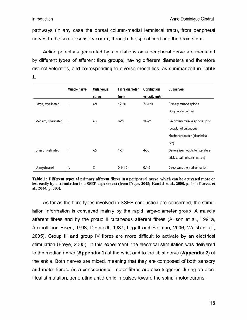
Action potentials generated by stimulations on a peripheral nerve are mediated
by different types of afferent fibre groups, having different diameters and therefore
distinct velocities, and corresponding to diverse modalities, as summarized in Table 1.
Muscle nerve Cutaneous
nerve
Fibre diameter
(μm)
Conduction
velocity (m/s)
Subserves
Large, myelinated I Aα 12-20 72-120 Primary muscle spindle
Golgi tendon organ
Medium, myelinated II Aβ 6-12 36-72 Secondary muscle spindle, joint
receptor of cutaneous
Mechanoreceptor (discrimina-
tive)
Small, myelinated III Aδ 1-6 4-36 Generalized touch, temperature,
prickly, pain (discriminative)
Unmyelinated IV C 0.2-1.5 0.4-2 Deep pain, thermal sensation
Table 1 : Different types of primary afferent fibres in a peripheral nerve, which can be activated more or less easily by a stimulation in a SSEP experiment (from Freye, 2005; Kandel et al., 2000, p. 444; Purves et al., 2004, p. 393).
As far as the fibre types involved in SSEP conduction are concerned, the stimu-
lation information is conveyed mainly by the rapid large-diameter group IA muscle
afferent fibres and by the group II cutaneous afferent fibres (Allison et al., 1991a,
Aminoff and Eisen, 1998; Desmedt, 1987; Legatt and Soliman, 2006; Walsh et al.,
2005). Group III and group IV fibres are more difficult to activate by an electrical
stimulation (Freye, 2005). In this experiment, the electrical stimulation was delivered
to the median nerve (Appendix 1) at the wrist and to the tibial nerve (Appendix 2) at
the ankle. Both nerves are mixed, meaning that they are composed of both sensory
and motor fibres. As a consequence, motor fibres are also triggered during an elec-
trical stimulation, generating antidromic impulses toward the spinal motoneurons.
18
Introduction Anne-Dominique Gindrat
Nevertheless, these potentials do not contribute to the brain stem and cortical
responses, contrary to fusorial afferences (Mauguière and Fischer, 1990).
Since the major target of both ascending pathways is S1, this region will be ex-
posed below in greater detail.
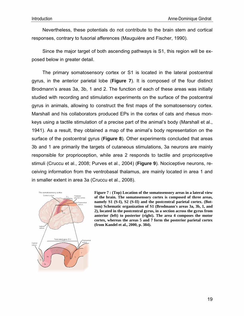
The primary somatosensory cortex or S1 is located in the lateral postcentral
gyrus, in the anterior parietal lobe (Figure 7). It is composed of the four distinct
Brodmann’s areas 3a, 3b, 1 and 2. The function of each of these areas was initially
studied with recording and stimulation experiments on the surface of the postcentral
gyrus in animals, allowing to construct the first maps of the somatosensory cortex.
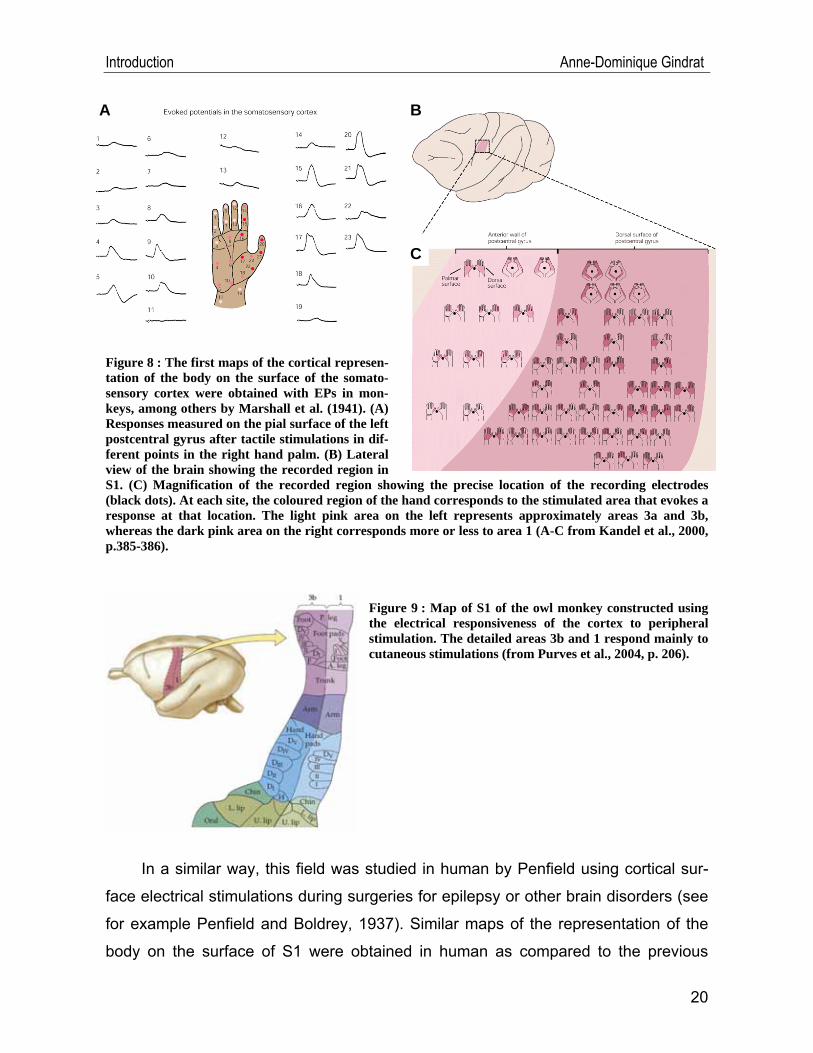
Marshall and his collaborators produced EPs in the cortex of cats and rhesus mon-
keys using a tactile stimulation of a precise part of the animal’s body (Marshall et al.,
1941). As a result, they obtained a map of the animal’s body representation on the
surface of the postcentral gyrus (Figure 8). Other experiments concluded that areas
3b and 1 are primarily the targets of cutaneous stimulations, 3a neurons are mainly
responsible for proprioception, while area 2 responds to tactile and proprioceptive
stimuli (Cruccu et al., 2008; Purves et al., 2004) (Figure 9). Nociceptive neurons, re-
ceiving information from the ventrobasal thalamus, are mainly located in area 1 and
in smaller extent in area 3a (Cruccu et al., 2008).
Figure 7 : (Top) Location of the somatosensory areas in a lateral view of the brain. The somatosensory cortex is composed of three areas, namely S1 (S-I), S2 (S-II) and the postcentral parietal cortex. (Bot-tom) Schematic organization of S1 (Brodmann's areas 3a, 3b, 1, and 2), located in the postcentral gyrus, in a section across the gyrus from anterior (left) to posterior (right). The area 4 composes the motor cortex, whereas the areas 5 and 7 form the posterior parietal cortex (from Kandel et al., 2000, p. 384).
19
Introduction Anne-Dominique Gindrat
Figure 8 : The first maps of the cortical represen-tation of the body on the surface of the somato-sensory cortex were obtained with EPs in mon-keys, among others by Marshall et al. (1941). (A) Responses measured on the pial surface of the left postcentral gyrus after tactile stimulations in dif-ferent points in the right hand palm. (B) Lateral view of the brain showing the recorded region in S1. (C) Magnification of the recorded region showing the precise location of the recording electrodes (black dots). At each site, the coloured region of the hand corresponds to the stimulated area that evokes a response at that location. The light pink area on the left represents approximately areas 3a and 3b, whereas the dark pink area on the right corresponds more or less to area 1 (A-C from Kandel et al., 2000, p.385-386).
C
BA
Figure 9 : Map of S1 of the owl monkey constructed using the electrical responsiveness of the cortex to peripheral stimulation. The detailed areas 3b and 1 respond mainly to cutaneous stimulations (from Purves et al., 2004, p. 206).
In a similar way, this field was studied in human by Penfield using cortical sur-
face electrical stimulations during surgeries for epilepsy or other brain disorders (see
for example Penfield and Boldrey, 1937). Similar maps of the representation of the
body on the surface of S1 were obtained in human as compared to the previous
20
Introduction Anne-Dominique Gindrat
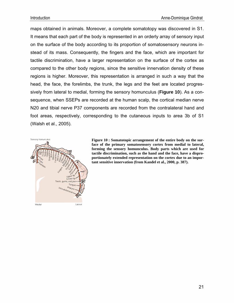
maps obtained in animals. Moreover, a complete somatotopy was discovered in S1.
It means that each part of the body is represented in an orderly array of sensory input
on the surface of the body according to its proportion of somatosensory neurons in-
stead of its mass. Consequently, the fingers and the face, which are important for
tactile discrimination, have a larger representation on the surface of the cortex as
compared to the other body regions, since the sensitive innervation density of these
regions is higher. Moreover, this representation is arranged in such a way that the
head, the face, the forelimbs, the trunk, the legs and the feet are located progres-
sively from lateral to medial, forming the sensory homunculus (Figure 10). As a con-
sequence, when SSEPs are recorded at the human scalp, the cortical median nerve
N20 and tibial nerve P37 components are recorded from the contralateral hand and
foot areas, respectively, corresponding to the cutaneous inputs to area 3b of S1
(Walsh et al., 2005).
21
7).
Figure 10 : Somatotopic arrangement of the entire body on the sur-face of the primary somatosensory cortex from medial to lateral, forming the sensory homunculus. Body parts which are used for tactile discrimination, such as the hand and the face, have a dispro-portionately extended representation on the cortex due to an impor-tant sensitive innervation (from Kandel et al., 2000, p. 38
Introduction Anne-Dominique Gindrat
II.3.4. Technique of SSEP recording in human3
In clinical studies on human, SSEPs are elicited either by a mechanical or an
electrical stimulation on the distal part of a peripheral nerve (Aminoff and Eisen,
1998). In the first case, for a tactile stimulation, a pneumatic stimulator can be used
on a finger (Wienbruch et al., 2006) (Figure 11A), but this technique requires more
stimulations than an electrical stimulation due to the small amplitude of the re-
sponses. In the latter case, transcutaneous electrical stimulations with a surface elec-
trode on the skin are delivered to afferent peripheral nerves, usually the median
(Figure 11B) or ulnar nerves at the wrist for upper extremity monitoring, and the pos-
terior tibial nerve at the ankle (Figure 11C) or the common peroneal nerve at the
knee for lower extremity monitoring (American Clinical Neurophysiology Society,
2006; Berger and Blum, 2007). The American Clinical Neurophysiology Society
(2006) recommends using monophasic rectangular pulses of 100-300μs duration at a
frequency of 3-5Hz. The stimulus intensity should be chosen so as to just produce a
small, visible, bearable twitch of the stimulated limb, e.g. an abduction of the thumb
in the case of a stimulation to the median nerve, and a plantar flexion of the toes after
a stimulation on the posterior tibial nerve (Aminoff and Eisen, 1998; Berger and
Blum, 2007; Cruccu et al., 2008). An earth electrode (a metal plate electrode, a
circumferential band electrode or a “stick-on” electrocardiographic-type electrode) is
placed on the stimulated limb, between the stimulation site and the recording site
(American Clinical Neurophysiology Society, 2006). During recording, it is recom-
mended to use a system bandpass of 5-30Hz and 2000-4000Hz for the low-and high-
frequency filters, respectively (American Clinical Neurophysiology Society, 2006;
Berger and Blum, 2007; Erwin et al., 1987; Freye, 2005).
3 Some information was also provided by http://emedicine.medscape.com/article/1137763-overview and http://emedicine.medscape.com/article/1139906-overview.
22
Introduction Anne-Dominique Gindrat
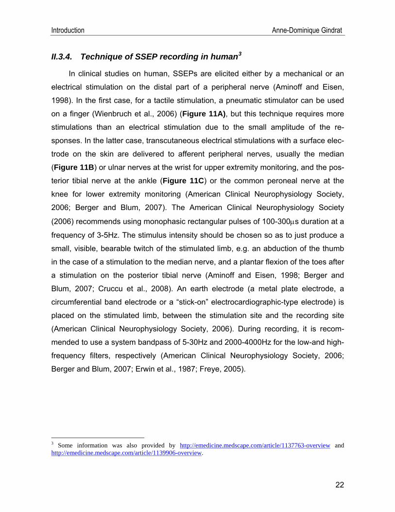
CA B
Figure 11 : (A) A pneumatic stimulation can be obtained with an air-puff stimulator on a finger. (B) To perform electrical stimulation to the median nerve at the wrist, the cathode is positioned about 2 cm proximal to the wrist crease, between the tendon of the M. Palmaris longus and M. flexor carpi radialis. The anode should be placed 2-3 cm distal to the cathode. (C) For electrical stimulation of the posterior tibial nerve, the cathode is positioned midway between the medial border of the Achilles tendon and the posterior border of the medial malleolus. The anode is placed 3cm distal to the cathode ((A) and (B) from Agustina Lascano, (C) from American Clinical Neurophysiology Society, 2006; Cruccu et al., 2008; Freye, 2005).
Responses can be recorded in a non-invasive way using standard EEG elec-
trodes (impedance: < 5kΩ) placed at the scalp, the cervical spine and close to the
peripheral stimulated nerve, i.e. at Erb’s point (angle formed by the posterior border
of the clavicular head of the sternomastoid muscle and the clavicule, 2-3cm above
the clavicule) when stimulating the median nerve or over the lumbosacral spine for
lower extremity stimulation (Cruccu et al., 2008; Freye, 2005). Minimal recommended
montage should be composed of four channels (Figure 12A, B) (American Clinical
Neurophysiology Society, 2006), but additional channels can be added along the
spine and at the scalp. High-resolution scalp recordings can be performed using a
cap with electrodes located according to the International 10-10 System (n=128 or
256) (Figures 13 and 14) (Lascano et al., 2009; Michel et al., 1999; van de Wassen-
berg et al., 2008). Examples of high-resolution SSEPs in human are shown in section
V.1.4. In fact, the channel number depends on what one wants to highlight: if the field
distribution is studied, high-resolution recordings are required, whereas in the case of
conduction time assessment, only some channels are needed (Aminoff and Eisen,
1998). Needle electrodes can also be used in order to reduce artefacts. To be sure
that recoded signals are not artefacts, it is recommended to replicate each recording
(American Clinical Neurophysiology Society, 2006; Cruccu et al., 2008). As the elec-
trical activity generated in cortical layers has to go through cerebrospinal fluid, men-
inges, the skull bone and the scalp, the amplitude of the propagating signal de-
creases and, as a consequence, the distribution of the signal becomes blurred
(Freye, 2005).
23
Introduction Anne-Dominique Gindrat
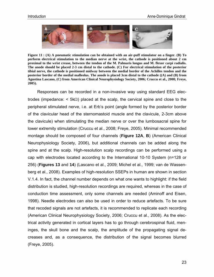
A B
Figure 12 : (A) For standard clinical SSEP recording by stimulating the median nerve at the wrist, a minimum of four channels is commonly used to highlight one or more particular components each: Chan-nel 1: Epi-Epc EP or N9, Channel 2: C5S-Epc N13, Channel 3: CPi-Epc P14 and N18, Channel 4: CPc-CPi N20. However, different other montages are also possible (see for example Cruccu et al., 2008). C5S: electrode over the fifth cervical vertebra; CPc: and CPi: centro-parietal cortex contralateral, respec-tively, ipsilateral, corresponding to Cz, respectively Pz positions of the International 10-20 system; Epc and Epi: Erb’s point contralateral, respectively ipsilateral to the stimulated limb. (B) Four channel mini-mally recommended montage for SSEP recording by stimulating the posterior tibial nerve: Channel 1: T12S-IC LP; Channel 2: Fpz-C5S P31 and N34; Channel 3: Cpz-Fpz P37; Channel 4: Cpi-Fpz P37. Different montages are also here possible. IC: iliac crest reference; LP: lumbar potential; T12S: electrode over the twelfth thoracic vertebra (from American Clinical Neurophysiology Society, 2006; Berger and Blum, 2007).
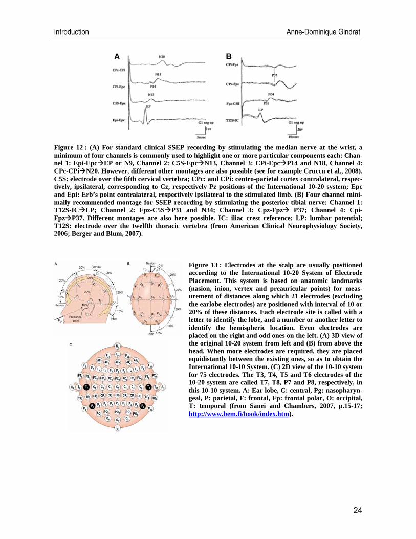
Figure 13 : Electrodes at the scalp are usually positioned according to the International 10-20 System of Electrode Placement. This system is based on anatomic landmarks (nasion, inion, vertex and preauricular points) for meas-urement of distances along which 21 electrodes (excluding the earlobe electrodes) are positioned with interval of 10 or 20% of these distances. Each electrode site is called with a letter to identify the lobe, and a number or another letter to identify the hemispheric location. Even electrodes are placed on the right and odd ones on the left. (A) 3D view of the original 10-20 system from left and (B) from above the head. When more electrodes are required, they are placed equidistantly between the existing ones, so as to obtain the International 10-10 System. (C) 2D view of the 10-10 system for 75 electrodes. The T3, T4, T5 and T6 electrodes of the 10-20 system are called T7, T8, P7 and P8, respectively, in this 10-10 system. A: Ear lobe, C: central, Pg: nasopharyn-geal, P: parietal, F: frontal, Fp: frontal polar, O: occipital, T: temporal (from Sanei and Chambers, 2007, p.15-17; http://www.bem.fi/book/index.htm).
24
Introduction Anne-Dominique Gindrat
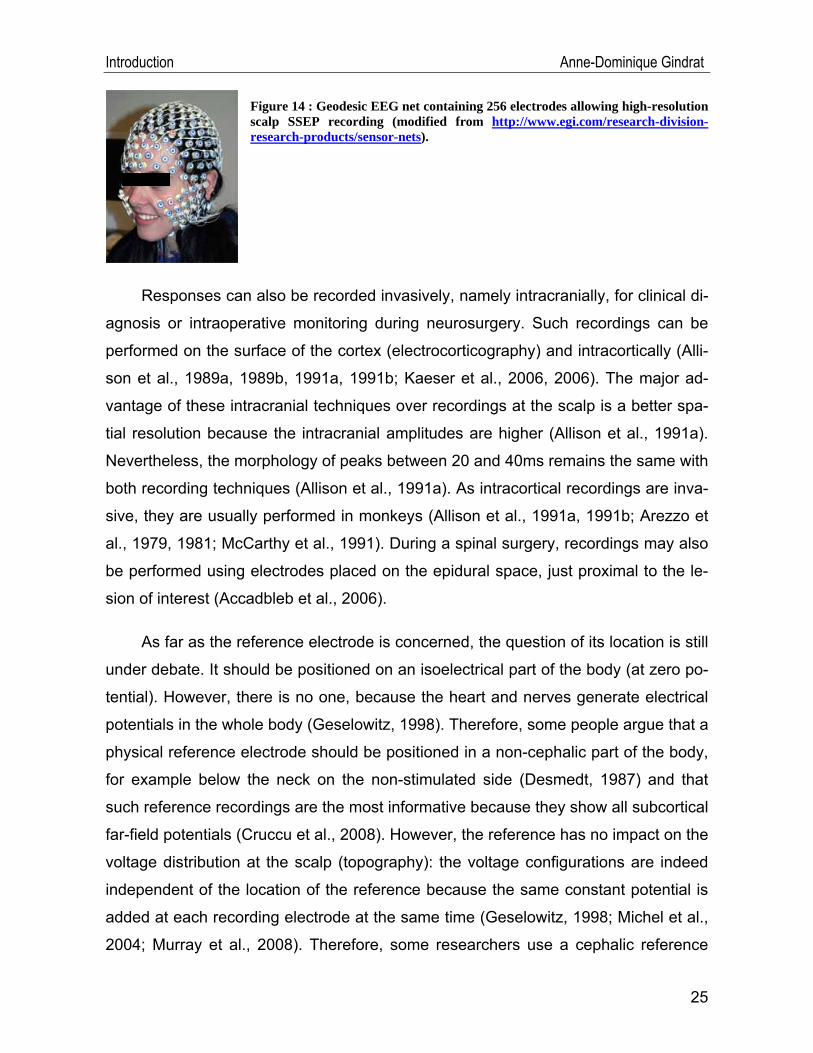
Figure 14 : Geodesic EEG net containing 256 electrodes allowing high-resolution scalp SSEP recording (modified from http://www.egi.com/research-division-research-products/sensor-nets).
Responses can also be recorded invasively, namely intracranially, for clinical di-
agnosis or intraoperative monitoring during neurosurgery. Such recordings can be
performed on the surface of the cortex (electrocorticography) and intracortically (Alli-
son et al., 1989a, 1989b, 1991a, 1991b; Kaeser et al., 2006, 2006). The major ad-
vantage of these intracranial techniques over recordings at the scalp is a better spa-
tial resolution because the intracranial amplitudes are higher (Allison et al., 1991a).
Nevertheless, the morphology of peaks between 20 and 40ms remains the same with
both recording techniques (Allison et al., 1991a). As intracortical recordings are inva-
sive, they are usually performed in monkeys (Allison et al., 1991a, 1991b; Arezzo et
al., 1979, 1981; McCarthy et al., 1991). During a spinal surgery, recordings may also
be performed using electrodes placed on the epidural space, just proximal to the le-
sion of interest (Accadbleb et al., 2006).
As far as the reference electrode is concerned, the question of its location is still
under debate. It should be positioned on an isoelectrical part of the body (at zero po-
tential). However, there is no one, because the heart and nerves generate electrical
potentials in the whole body (Geselowitz, 1998). Therefore, some people argue that a
physical reference electrode should be positioned in a non-cephalic part of the body,
for example below the neck on the non-stimulated side (Desmedt, 1987) and that
such reference recordings are the most informative because they show all subcortical
far-field potentials (Cruccu et al., 2008). However, the reference has no impact on the
voltage distribution at the scalp (topography): the voltage configurations are indeed
independent of the location of the reference because the same constant potential is
added at each recording electrode at the same time (Geselowitz, 1998; Michel et al.,
2004; Murray et al., 2008). Therefore, some researchers use a cephalic reference
25
Introduction Anne-Dominique Gindrat
and re-compute then the results against the average reference to respect the quasi-
stationarity (the net source of the head must be zero) (Michel et al., 2004; Murray et
al., 2008).
II.3.5. SSEP components4
The peaks of the different SSEP components are called according to their polar-
ity (N for negative and P for positive) and their average post-stimulus latency from a
sample of the normal adult population (American Clinical Neurophysiology Society,
2006; Berger and Blum, 2007; Cruccu et al., 2008; Desmedt, 1987; Gilmore, 1989;
Mauguière and Fischer, 1990). Let’s take P20 as an example: this peak is positive
and appears 20ms after the stimulus. Conversely, N20 is a negative peak. However,
in some cases, the latency does not perfectly correspond to the name of the compo-
nent, given that the latency is influenced by the length of the somesthesic pathways
which depends on the patient’s stature (Desmedt, 1987).
One can also distinguish between near-field and far-field EPs according to the
distance of their source with the recording electrodes. Near-field potentials refer to
long-latency cortical components produced by generators located in the grey matter
of perirolandic cortical areas, within 3-4 cm from the recording electrodes. These po-
tentials show a small spread, a steep lateral gradient and a topographical specificity,
meaning that they show morphological variations when they are recorded from differ-
ent locations at the scalp. On the other hand, far-field potentials correspond to
SSEPs whose generators are subcortical or peripheral, in the white matter, and are
thus more distant from the scalp and have a shorter latency than near-field compo-
nents. These responses are characterized by a wide spread, a shallow gradient and
a relative topographical nonspecificity (Banoub et al., 2003; Berger and Blum, 2007;
Desmedt, 1987; Erwin et al., 1987; Freye, 2005; Gilmore, 1989; Mauguière and
Fischer, 1990).
SSEPs are generally classified according to their latency. When only consider-
4 Some information was also provided by http://emedicine.medscape.com/article/1139906-overview.
26
Introduction Anne-Dominique Gindrat
ing the electrical stimulations delivered to the human median nerve, short-latency
SSEPs appear in a meantime of 20ms to 40ms after the stimulation and are gener-
ated by subcortical structures. On the contrary, long-latency SSEPs are recorded
from 40ms to 250ms after the stimulation and are the result of cortical generators (Al-
lison et al., 1989a, 1989b, 1991a; Freye, 2005). Some authors however categorize
them as short-latency (from 10ms to 40ms post-stimulation), intermediate-latency
(from 20ms to 120ms post-stimulation) and long-latency potentials (from 250ms post-
stimulation) (Umamaheswara, 2002).
Human characteristic short-latency peaks produced after stimulation of the me-
dian nerve are among others N9, P9, N11, P11, N13, P13, P14, N18, N20, P20, P22,
P25, P27, N30, P30, N35, P45 (Figure 12A) (Desmedt, 1987, Mauguière and
Fischer, 1990).
The first peak, a near-field potential called EP or N9, is recorded at Erb’s point
and gives information about the activity generated within the brachial plexus. P9 is
very likely also generated within the brachial plexus (Desmedt, 1987). Both of these
components are thus peripheral. P11 and N11, which are measured over the lower
cervical spine, show the activity in the primary somesthesic neuron near the dorsal
root entry zone in the spinal cord (Desmedt, 1987). N13, a near-field stationary po-
tential measured over the lower cervical spine, and P13, measured using an oeso-
phageal electrode, probably correspond to postsynaptic activity of neurons in the
posterior horn of the lower cervical spinal cord and in ascending afferents in the
cuneate tract (American Clinical Neurophysiology Society, 2006; Berger and Blum,
2007; Desmedt, 1987). It seems that P14, a subcortically generated far-field potential
recorded referentially from the scalp and having a widespread distribution, is the re-
sult of activity in the dorsal column nuclei or the caudal medial lemniscus (American
Clinical Neurophysiology Society, 2006). One proposes that N18, a subcortically
generated far-field potential recorded referentially from ipsilateral scalp electrodes, is
due to postsynaptic activity in the brain stem and the thalamus (American Clinical
Neurophysiology Society, 2006). N20 is a near-field potential derived over the contra-
lateral parietal cortex and it is the first cortical negativity, reflecting activation in con-
27
Introduction Anne-Dominique Gindrat
tralateral S1 from thalamocortical radiations projecting from the VPL (American Clini-
cal Neurophysiology Society, 2006; Berger and Blum, 2007; Desmedt, 1987). P22 is
produced by a frontal generator located near the central sulcus (Desmedt, 1987, Er-
win et al., 1987). The P20-N30 group is primarily recorded over the motor cortex and
the frontal scalp, the N20-P30 group over S1 and the parietal scalp and the group
P25-N35 near the central sulcus and the central scalp (Allison et al., 1991a). N20,
P20, P25, N30 P 30 and N35 are the result of activity of neurons located in the hand
area of contralateral S1 and in cortical association areas (Erwin et al., 1987).
When high-resolution median nerve SSEPs are acquired at the human scalp
(see Figure 50, section V.1.4), N15 is recorded on the neck and corresponds to ac-
tivity most probably generated in the dorsal column nuclei in the brain stem. Later,
N20 is supposed to be generated by a tangential dipole in area 3b. P27 is recorded
from the contralateral hemisphere and corresponds to an activation of the hand area
in the sensorimotor cortex (Lascano et al., 2009; van de Wassenberg, 2008a).
First human obligatory short-latency peaks produced following the stimulation of
the posterior tibial nerve are among others N18, LP, P31, N34, and P37 (Figure 12B) (American Clinical Neurophysiology Society, 2006).
N18 is a travelling wave recorded over the lower lumbar spine just after the sac-
ral plexus. This signal is recorded at the scalp as the far-field potential P18. The sec-
ond peak is called LP or N22 and is recorded referentially over the dorsal lower tho-
racic and upper lumbar spine. It is a stationary potential corresponding to activity in
the dorsal root, the dorsal root entry zone and to postsynaptic activity in the lumbar
cord enlargement. It is analogous to the cervical component N13 recorded after me-
dian nerve stimulation (American Clinical Neurophysiology Society, 2006; Berger and
Blum, 2007). N29, a far-field component, seems to be generated by neurons in the
gracile nucleus. P31, another far-field response, is probably due to activity in the dor-
sal column nuclei and/or the caudal medial lemniscus in the lower medulla. It is
analogous to P14 peak of the median nerve SSEPs. N34, recorded referentially from
frontal electrodes, is a subcortically generated far-field potential possibly revealing
postsynaptic activity in the brain stem and/or in the thalamus, like N18 potential pro-
28
Introduction Anne-Dominique Gindrat
29
duced in median nerve SSEPs (American Clinical Neurophysiology Society, 2006).
P37 is a near-field potential corresponding to activation in somatosensory receiving
areas (American Clinical Neurophysiology Society, 2006; Erwin et al., 1987).
When high-resolution tibial nerve SSEPs are acquired at the human scalp (see
Figure 51, section V.1.4), P39 can be recorded from centro-parietal electrodes (van
de Wassenberg, 2008b).
II.3.6. Cortical SSEP generators5
It is essential to identify the different generators for a correct interpretation of the
observed waveforms (Berger and Blum, 2007). The numerical cartography of the
EPs fields attempted to locate some SSEP generators in monkeys and in human.
However, this approach caused many debates (Allison et al., 1989a, 1991a; Arezzo
et al., 1981, Desmedt, 1987; McCarthy et al., 1991).
It has been proposed that P10-N20 and N10-P20 median nerve SSEPs in the
anaesthetized monkey and P20-N30 and N20-P30 in human result from a tangential
generator located in the posterior bank of the central sulcus, i.e. in the area 3b of
contralateral S1. This generator produces potentials whose amplitude decreases as
the distance with the central sulcus increases (Allison et al., 1991a).
P12-N25 in the anaesthetized monkey and P25-N35 in human are produced
some milliseconds after by a generator that is radially oriented in the contralateral
cortical areas 1 and 2 in S1. When these potentials are recorded on the surface of
the cortex, one can observe an inversion of polarity as compared to the recording in-
side the white matter (Allison et al., 1991a).
Allison et al. (1989b) demonstrated that there are long-latency potentials in hu-
man (from 40 ms to 250 ms). In the same way as short-latency ones, they are gener-
ated in contralateral areas 3b and 1 of S1, but also in other areas of S1, in S2 as well
as in the ipsilateral hemisphere.
5 Some generators were already described in the previous section.
Introduction Anne-Dominique Gindrat
The responses P37 and N37 generated after tibial nerve stimulation in human
are produced in the leg representation of contralateral S1, in the medial aspect along
the longitudinal cerebral fissure (Figure 10). The cortical generator is a horizontal di-
pole with the positive tail toward the ipsilateral parietal cortex and negative tail toward
the contralateral fronto-temporal region. Accordingly, the highest amplitude positivity
(P37) is often recorded ipsilaterally one or two centimetres lateral to the midline,
whereas the negative component is derived from the contralateral hemisphere (Ber-
ger and Blum, 2007; Cruccu et al., 2008; Erwin et al., 1987).
The next tibial component, P39, derived with the highest amplitude on the ipsi-
lateral parietal cortex, is produced by a generator with a more vertical, quite oblique
orientation in the inter-hemispheric fissure (Cruccu et al., 2008).
Nowadays, with high-resolution SSEP recordings, the location of the generator
can be determined by solving an inverse solution (Michel et al., 1999, 2001, 2004).
II.3.7. Similarities between human and monkey SSEPs
In two studies, Arezzo et al. (1979, 1981) showed that in rhesus monkeys
Macaca mulatta, early components (with a latency shorter than 15ms in human),
generated from the peripheral nerve to the thalamocortical radiations, as well as cor-
tical components of SSEPs, resemble in configuration and topography the human
components. Nevertheless, the latencies recorded in monkeys are about 10ms
shorter than the human ones because somesthesic pathways in rhesus monkeys are
shorter (Allison et al., 1991a; Desmedt, 1987). For example, the cortical components
P10-N20, N10-20 and P12-N25 in macaques and in Old World monkeys correspond
to human potentials P20-N30, N20-P30 and P25-N35, respectively (Allison et al.,
1989a, 1991a, 1991b; McCarthy et al., 1991) (Figure 15). These results suggest that
the same neuronal activity and topography are conserved between both species.
30

Introduction Anne-Dominique Gindrat
Figure 15 : Comparison of short-latency SSEPs evoked by stimulation of the contralateral median nerve, in human and the monkey. Cortical-surface recordings were performed in the right sensorimotor cortex of anaesthetized human and monkey. The grey area of monkey’s cortex represents the hand area in S1. AS : arcuate sulcus, CS : central sulcus, IPS : intraparietal sulcus, LS : lateral sulcus, PrCS : precentral sulcus, PoCS : postcentral sulcus, SPS : superior precentral sulcus. The stimulus was deliv-ered at 0 ms (from McCarthy et al., 1991).
II.3.8. Clinical applications
Nowadays, the clinical usefulness of EPs has changed due to the emergence of
imaging techniques such as the MRI. However, whereas MRI gives anatomical and
structural information with a good spatial resolution, EPs provide functional and
physiological explanations of some pathways of the nervous system with excellent
temporal resolution. Consequently, both theses techniques are complementary. In
fact, when MRI does not provide a clear diagnosis, neurologists have recourse to
EPs, as in case of ambiguous diagnosis of multiple sclerosis, for instance.
In the clinic, the amplitude, latency and morphology of the peaks are checked
and compared with the norms obtained from a healthy population. The most impor-
tant indications of SSEP abnormality are changes from the baseline responses, the
absence of an obligatory peak and the abnormal prolongation of the interpeak la-
tency (American Clinical Neurophysiology Society, 2006; Berger and Blum, 2007).
The peak and interpeak latencies are considered to be abnormal if they are more
than 3 standard deviations above the normal mean (Aminoff and Eisen, 1998; Carter
et al., 1999; Cracco, 1989; Freye, 2005). As amplitudes show a high inter-individual
variability, they do not have a high clinical value (Berger and Blum, 2007). It is how-
ever possible that a patient suffering from a neurological disorder presents no altera-
tion in SSEPs given that the information is processed by several parallel pathways
(Cruccu et al., 2008; Freye, 2005).
31
Introduction Anne-Dominique Gindrat
EP recording is clinically very relevant because it is a method allowing diagnos-
ing many neurological disorders affecting the somatosensory conduction, by testing
the integrity of somatosensory function along peripheral nerves, plexus, dorsal radix
of spinal nerves, the spinal cord, the brain stem, the thalamus and lastly the sensory
cortex (Aminoff and Eisen, 1998; Berger and Blum, 2007; Cruccu et al., 2008; Erwin
et al., 1987; Freye, 2005; Mauguière, 2005; Mauguière and Fischer, 1990). EPs give
information about the location of spinal injuries, pathologies, lesions, tumours, de-
generations, abnormalities in synaptic transmission or demyelination in the central
and peripheral nervous system (Berger and Blum, 2007; Cruccu et al., 2008; Erwin et
al., 1987; Freye, 2005; Mauguière, 2005; Mauguière and Fischer, 1990; Walsh et al.,
2005). These clinical diagnoses are often obtained with median nerve SSEPs com-
bined with tibial nerve SSEPs. These latter have the advantage of assessing the in-
tegrity of much of the length of the spinal cord as compared to the first (Aminoff and
Eisen, 1998). Given that the generators have different locations, short-latency poten-
tials are used to check the integrity of the nerves, the spinal cord and the brain stem.
On the other hand, long-latency potentials allow investigating the cerebral cortex
(Mauguière and Fischer, 1990).
In the past, a major application was the diagnosis and progression monitoring of
multiple sclerosis in peripheral and central nervous system (Erwin et al., 1987; Gi-
esser, 1993; Regan, 1989; Walsh et al., 2005). However, the diagnosis is today pref-
erentially obtained with MRI. Physicians only have recourse to SSEPs and other mo-
dalities EPs in the case of equivocal diagnosis after MRI, or in the case of clinically
unsuspected lesions (Aminoff and Eisen, 1998; Berger and Blum, 2007; Cruccu et
al., 2008; Erwin et al., 1987; Gronseth and Ashman, 2000; Kallmann et al., 2006;
Walsh et al., 2005). SSEPs are also used to investigate patients affected by possible
Friedreich’s ataxia, leukodystrophies or myoclonus (Aminoff and Eisen, 1998; Daw-
son, 1947b; Erwin et al., 1987; Regan, 1989, Walsh et al., 2005). This method is also
helpful to evaluate the regeneration of sensitive axons, to calculate afferent conduc-
tion rates using latency differences, and thereby to detecting sensory system conduc-
tion abnormalities (Desmedt, 1987; Freye, 2005; Mauguière, 2005; Mauguière and
32
Introduction Anne-Dominique Gindrat
Fischer, 1990; Regan, 1989, Walsh et al., 2005).
The major use of SSEPs is the intraoperative monitoring. During orthopaedic,
neurological or vascular surgeries, the recorded SSEPs are used to locate the sen-
sorimotor cortex and the central sulcus (the human postcentral N20 shows a polarity
reversal to a precentral P20), to functionally monitor in real-time a possible anoxia,
ischemia or mechanical damage of the somatosensoriel pathway, to assess the con-
duction or to continuously monitor the integrity of the sensory pathways during surgi-
cal correction of spinal curvatures, vertebral surgery or tumour resection, for example
(Berger and Blum, 2007; Cruccu et al., 2008; Erwin et al., 1987; Freye, 2005; Gonza-
les et al., 2009; Regan, 1989; Tan and Lo, 2003; Walsh et al., 2005). They are also
relevant to assess the depth of anaesthesia by monitoring the presence of late corti-
cal components, given that they are more affected by anaesthesia than earlier ones
(Vaughan et al., 2001). Moreover, they are helpful in the intensive care unit to evalu-
ate the neurological status of a coma patient or a brain-dead suspected patient after
a trauma, an anoxia or an ischemia, for example, as exposed in greater detail just
below (Aminoff and Eisen, 1998, Macado, 1996; Mauguière and Fischer, 1990;
Regan, 1989, Walsh et al., 2005).
Since the 1980es, the predictive value of SSEPs in long-term outcome after a
central nervous system injury is being assessed and discussed. Among others, the
study of Gott et al. (1990) showed that SSEPs are disrupted in patients affected by a
cerebral ischemia. However, they concluded that this approach is not better than a
precise clinical examination to predict the outcome from a stroke. Moreover, although
SSEPs help to predict communication improvements and motor recovery, this elec-
trophysiological method was shown not to be a sufficient predictor of the outcome
after a stroke in dominant hemisphere (Keren et al., 1993). Later, a study of Feys et
al. (2000) indicated that primarily SSEPs measured in the acute phase are the best
predictors of arm recovery at 6 and 12 months after stroke when they are combined
with motor performance evaluation. However, the SSEP prognosis value of the long
term outcome decreased when measured at 2 months in aid of MEPs combined with
motor performance measurements. Other studies also related the better predictive
33

Introduction Anne-Dominique Gindrat
value to a malignant course of other modalities EPs (BAEPs) in acute phase after a
stroke as compared to SSEPs (Burghaus et al., 2008; Machado, 1996).
Nevertheless, Carter and Butt (2001, 2005) reviewed the literature covering this
subject and demonstrated that SSEPs are the best single predictor of the level of re-
covery in patients after a serious cerebral damage, such as a stroke for example.
Moreover, other previous studies, such as Carter et al. (1999) or Lew et al. (2003),
go in the same direction, namely that SSEPs are good predictor for short-term and
long-term outcome after a brain injury, primarily of poor outcome (vegetative state or
death). In conclusion, the use of SSEPs in the prediction of outcome after brain dam-
age remains under debate.
Besides their easiness to be performed and the fact that they can be more sen-
sitive than a neurological examination, a great advantage of SSEPs over sensory ex-
amination is their objectivity (Zeman and Yiannikas, 1989, Walsh et al., 2005). Fur-
thermore, they provide quantitative results, which represent additional information to
the clinical neurological examination (Cruccu et al., 2008; Walsh et al., 2005; Zeman
and Yiannikas, 1989), in adults, as well as in children (Cracco, 1989; Gilmore, 1989;
Regan, 1989). Last but not least, they can be used in almost all clinical situations,
e.g. in unconscious, comatose or paralyzed patients, or in patients under sedatives,
muscle relaxants or anaesthetic drugs (Carter and Butt, 2001; Carter et al., 1999;
Walsh et al., 2005; Zeman and Yiannikas, 1989).
Despite all these characteristics, SSEPs also have some disadvantages in the
clinical use, namely they are not always disease specific; it is possible that they are
confounded by end organ disease; they are affected by age and it is necessary that
the patient remains quiet in order to avoid artefacts during recordings (Walsh et al.,
2005).
Following a lesion of the centro-parietal cortex, cortical pre- and retrorolandic
responses disappear on the lesioned side while far-field components as well as N18
are conserved. When the lesion affects the sensorimotor cortex in the central region,
some postrolandic components are lost and the patient presents some sensitivity
34
Introduction Anne-Dominique Gindrat
35
disorders. Finally, when the lesion only concerns prerolandic components, the patient
keeps a normal sensitivity but his mobility is impaired (Mauguière and Fischer, 1990).
II.3.9. Factors altering the evoked responses
The latency, amplitude, morphology and topographical distribution of SSEPs
can be influenced by several parameters. Besides the pathologic factors described
above, the stimulation parameters play a role (Banoub et al., 2003; Freye, 2005). In-
deed, the response can change with:
• the type of stimulation: an electrical stimulation produces a higher ampli-
tude response than a mechanical stimulation (Aminoff and Eisen, 1998).
• the stimulus intensity: The latency of median nerve SSEPs are not affected
by changes of the stimulation intensity, whereas the amplitude rises with an
increase of the intensity until an thumb twitch is perceptible. The amplitude is
maximal at a slightly supra-liminar stimulation intensity (Mauguière and
Fischer, 1990). But if the stimulation intensity is too high, an occlusion of Ia
impulse traffic is generated by other converging afferent signals (Aminoff and
Eisen, 1998). In this case, some of the first afferent volleys are ineffective,
decreasing the amplitude of the signal.
• the stimulus frequency: Neither changes the latency with an increase of
the stimulation frequency. However, the amplitude declines as the frequency
increases, especially in young children (Araki et al., 1999). Cases of neu-
ronal adaptation were reported for example in rodents after whisker stimula-
tion when the frequency was greater than 0.5 stimulation/s (Quairiaux et al.,
2007). In this case, a constant response amplitude was reached after 3 or 4
stimulations.
• the filter setting
• the stimulated level along the peripheral nerve
Introduction Anne-Dominique Gindrat
Equally important, subject parameters are involved (Freye, 2005), such as:
• the age: it has been shown that aging induces a gradual increase of the am-
plitude and latency of SSEPs in healthy people (Aminoff and Eisen, 1998;
Shagass and Schwartz, 1965; Zumsteg and Wieser, 2002). Peripheral
nerves are more affected by age than central ones. The conduction velocity
at the median nerve decreases by about 0.16m/s/year, meaning that the la-
tencies increase. In young human adults, peripheral conduction is 71.1±4.0
m/s, whereas it decreases to 61.2±5.9m/s in healthy octogenarians (Des-
medt, 1987). By comparison, the rate of the central conduction remains sta-
ble until 60 years old; then it decreases (0.78m/s/year). Aging also has an ef-
fect on the spatial distribution of SSEPs (Mauguière, 2005; Mauguière and
Fischer, 1990; Zumsteg and Wieser, 2002).
• the maturation: SSEPs can also be recorded in infants. As their nervous
system is still maturing (Berger and Blum, 2007; Gilmore, 1989), the inter-
peak latency after a stimulation to the median nerve decreases first rapidly
from age 0 to 2 years old, then slower from 2 to 6 years old, and reaches
adult values at 8 years old. As far as stimulation to the tibial nerve is consid-
ered, children reach the adult peripheral and central conductions at 3 years
old, respectively 5 years old.
• the gender: As females are usually shorter than males, the latency of me-
dian nerve SSEPs is 1ms shorter in the former than in the latter in central
conduction.
• the height: the length of the somesthesic pathways increase with the pa-
tient’s height and consequently the latency increases as well in adults (Mau-
guière and Fischer, 1990). This factor is more marked for lower than upper
limb stimulation (Mauguière, 2005).
• the cutaneous and core temperatures: the temperature affects mainly the
limbs where the conduction increases as the temperature rises (5% per
1°C), whereas the effects on the central pathways are minor. In case of in-
creasing hypothermia, central conduction time and latency lengthen, and
some components tend to disappear (Banoub et al., 2003; Mauguière,
36
Introduction Anne-Dominique Gindrat
2005). Conversely, a hyperthermia results in a decrease of the conduction
time and latency, whereas the amplitude is not affected (Banoub et al.,
2003). Consequently, the recordings should be performed at constant tem-
perature (21-23°C), with the cutaneous temperature at 34°C and the central
body temperature at 37°C.
• the consciousness degree: the amplitude, latency and waveform of some
components such as human N20 are subject to changes during the different
stages of sleep and vigilance (Mauguière, 2005).
• the attention: some early cortical components before 50 ms could be modi-
fied by attention-related processes (Mauguière, 2005).
• the blood pressure: a drop in patient blood pressure can result in a slight
reduction of the amplitude (Banoub et al., 2003; Tan and Lo, 2003).
• an anaesthesia administration (Banoub et al., 2003): The diverse SSEPs
components are differently affected by anaesthesia: whereas subcortical
SSEPs are not disrupted, the sensitivity of middle-latency cortical SSEPs to
anaesthesia increases and longer latency cortical components are extremely
susceptible to anaesthetics (Berger and Blum, 2007; Vaughan et al., 2001).
As a consequence, the more resistant, subcortical components are generally
used for intraoperative monitoring.
Generally, intravenous anaesthetics have a smaller depressive effect on
SSEPs than gas anaesthetics. At high dose, one can observe a small in-
crease of latency and a small decrease of amplitude (Table 2). Large dose
injection of ketamine, however, induces an increase in cortical SSEP ampli-
tude from 2 to 10 minutes after administration, without any evident effect on
the latency of cortical or subcortical components (Detsch and Kochs, 1997).
The volatile anaesthetics such as sevoflurane, the other anaesthetic used in
this study, act in a dose-dependant manner by increasing the SSEP latency
and the central conduction time, and by decreasing the amplitude (Table 3)
(Boisseau et al., 2002, Schwender et al., 1998). They also induce morpho-
logical changes of the peaks (Rehberg et al., 1998). Moreover, whereas
subcortical components are minimally affected, the later cortical responses
37
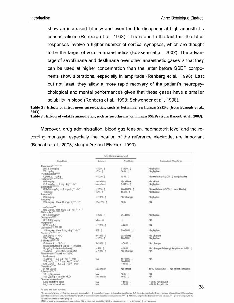
Introduction Anne-Dominique Gindrat
show an increased latency and even tend to disappear at high anaesthetic
concentrations (Rehberg et al., 1998). This is due to the fact that the latter
responses involve a higher number of cortical synapses, which are thought
to be the target of volatile anaesthetics (Boisseau et al., 2002). The advan-
tage of sevoflurane and desflurane over other anaesthetic gases is that they
can be used at higher concentration than the latter before SSEP compo-
nents show alterations, especially in amplitude (Rehberg et al., 1998). Last
but not least, they allow a more rapid recovery of the patient’s neuropsy-
chological and mental performances given that these gases have a smaller
solubility in blood (Rehberg et al., 1998; Schwender et al., 1998). Table 2 : Effects of intravenous anaesthetics, such as ketamine, on human SSEPs (from Banoub et al., 2003). Table 3 : Effects of volatile anaesthetics, such as sevoflurane, on human SSEPs (from Banoub et al., 2003).
Moreover, drug administration, blood gas tension, haematocrit level and the re-
cording montage, especially the location of the reference electrode, are important
(Banoub et al., 2003; Mauguière and Fischer, 1990).
38
Introduction Anne-Dominique Gindrat
39
II.4. Goals of the present study
As exposed briefly at the beginning, the first aim was to develop a non-invasive
method allowing repeated monitoring of cerebral activity in macaque monkey in rela-
tion to a cortical or subcortical lesion, hence the use of SSEPs. To this aim, a trans-
position of multichannel (n= 128 or 256) EP recordings at human scalp (Lascano et
al., 2009) was performed to monkeys with an EEG cap containing a reduced number
of channels (n=32, due to the small size of the head).
Introduction Anne-Dominique Gindrat
The purpose was to make improvements to a previously used approach by
Kaeser et al. (2006, 2007) in the laboratory, with SSEP recordings restricted to 16
electrodes above the premotor cortex (PM), S1 and the primary motor cortex (M1).
This method was limited because of the restricted area of the brain which was inves-
tigated and consequently, the reorganization at long distance could not be seen.
To develop the recording technique and test its validity, we will concentrate on
the evaluation of the stability of SSEPs responses obtained in similar conditions.
First, we will consider the stability of the individual sweeps within a recording. Then,
we will assess the stability of SSEPs obtained in the same session with the same
stimulation, then in the same session by repositioning the stimulator between acquisi-
tions to evaluate this effect. Finally, we will test the reproducibility of the responses
across different sessions. Then, the following recording parameters will be tested: the
stimulation frequency, the number of sweeps to average, the stimulation intensity, the
type of anaesthesia and its dosage. The results will be analysed classically in terms
of peaks as well as in terms of scalp topography, a method not applied in monkey
yet. At the end, we will present typical median nerve SSEPs and tibial nerve SSEPs
obtained with this new established protocol.
.
40
Material and methods Anne-Dominique Gindrat
III. Material and methods Experiments were conducted on one young adult male macaque monkey
(Macaca fascicularis)6 aged between 4 years 7 months and 5 years 7 months old
(body weight: 3.0kg to 4.9kg), living with two other congeners in a 15m3 room (12
hours light/12h hours dark cycle). The weight of the animal was checked daily. The
animal was on no account food- or water-deprived. All procedures and animal care
were conducted in accordance with the Guide for Care and Use of Laboratory Ani-
mals (ISBN 0-309-05377-3; 1996) and were approved by local (Swiss) veterinary au-
thorities. Experimental procedures were designed to minimize the animal’s pain and
suffering.
III.1. SSEP acquisition and analysis
III.1.1. Anaesthesia and procedure
In the first series of experiments, in order to facilitate the installation of the EEG
cap and the subsequent recordings, the monkey was anaesthetized with a mix of one
volume of Ketasol-100® (K) (Graeub, ketamine hydrochloride, 100mg/ml) and one
volume of Domitor® (D) (Pfizer, medetomidine hydrochloride, 1.0 mg/ml) (0.1 ml/kg,
i.m.). The head of the monkey was then shaved off and washed with alcohol so as to
eliminate the insulating film produced by some fat excess. After that, the monkey was
placed in a chair (designed by Florian Lanz) with the forearms on arm-rests and the
hindlimbs laying horizontally on a support. Its back and nape of the neck were main-
tained in an adequate position with a customized thermoplastic shell (Turbocast
without perforation, Art.-nr 636025, FREY Orthopädie-Bedarf AG, Othmarsingen,
CH) (Figure 17A,, p.44). The EEG cap was then positioned at the scalp of the mon-
key and maintained in the correct position using a chin belt. Deep anaesthesia was
maintained for the whole recording session with subsequent reinjections of the mix of
K+D. After the recordings had been finished, the monkey received an injection of An-
6 For more information, see http://pin.primate.wisc.edu/factsheets/entry/long-tailed_macaque and Bonadio (2000).
41
Material and methods Anne-Dominique Gindrat
42
tisedan® (Pfizer, atipamezole hydrochloride, 5.0mg/ml) (0.05ml/kg, i.m.) in order to
facilitate its waking up.
Subsequently, in a second series of experiments, the protocol was improved:
the monkey was first pre-anaesthetized for about 60-80 minutes with an injection of
the mix of K+D or D only, to allow the shaving, the installation of the monkey and the
positioning of the cap. After that, Antisedan® was administrated and the monkey was
let to regain some level of consciousness. Before the monkey was totally awake, a
gas anaesthesia was induced with Sevorane® (Abbott, sevoflurane) delivered with a
mask by a vaporizer (Vapor 19.3®, Drägerweck AG, Lübeck, Germany). To this aim,
a bolus was given first with a concentration of 5% of sevoflurane (2ℓ/min air; 0.5ℓ/min
O2) for about 10 minutes. Then, the concentration of sevoflurane was progressively
reduced and maintained at 2.5% (2ℓ/min air; 0.5ℓ/min O2) for the rest of the experi-
ment. At the end of the recordings, the sevoflurane anaesthesia was stopped and the
monkey received oxygen at the mask to wake him up.
The protocol underwent a last improvement in the third series of experiments to
obtain a stable anaesthesia level during the recording session: one to three days be-
fore the recordings, if necessary, the scalp of the monkey was shaved off under an-
aesthesia (mix of K+D). On the SSEP recording day, the monkey was directly anaes-
thetized with sevoflurane, without any pre-anaesthesia. In order to obtain a rapid an-
aesthesia, a bolus was given at a concentration of about 6-7% (5ℓ/min air; 1.25ℓ/min
O2) of sevoflurane for about 5 minutes. Then, the concentration was progressively
reduced and maintained at 2.5% (2ℓ/min air; 0.5ℓ/min O2) for the continuation of the
experiment (scalp cleaning, installation of the monkey, positioning of the cap and re-
cordings). In some recording sessions, at the end, the level of gas was even reduced
to 1.5% (2ℓ/min air; 0.5ℓ/min O2) for about the last 40 minutes. At the end of the re-
cordings, the sevoflurane anaesthesia was stopped and the monkey received oxygen
at the mask to wake him up.
All these SSEP recordings were performed in a Faraday cage room in order to
avoid interferences with other electrical fields provoking noise.
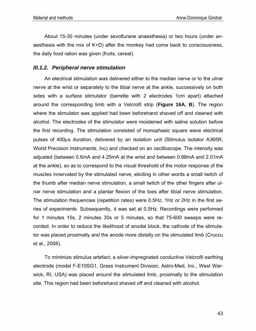
Material and methods Anne-Dominique Gindrat
About 15-30 minutes (under sevoflurane anaesthesia) or two hours (under an-
aesthesia with the mix of K+D) after the monkey had come back to consciousness,
the daily food ration was given (fruits, cereal).
III.1.2. Peripheral nerve stimulation
An electrical stimulation was delivered either to the median nerve or to the ulnar
nerve at the wrist or separately to the tibial nerve at the ankle, successively on both
sides with a surface stimulator (barrette with 2 electrodes 1cm apart) attached
around the corresponding limb with a Velcro® strip (Figure 16A, B). The region
where the stimulator was applied had been beforehand shaved off and cleaned with
alcohol. The electrodes of the stimulator were moistened with saline solution before
the first recording. The stimulation consisted of monophasic square wave electrical
pulses of 400μs duration, delivered by an isolation unit (Stimulus isolator A365R,
World Precision Instruments, Inc) and checked on an oscilloscope. The intensity was
adjusted (between 0.6mA and 4.25mA at the wrist and between 0.88mA and 2.01mA
at the ankle), so as to correspond to the visual threshold of the motor response of the
muscles innervated by the stimulated nerve, eliciting in other words a small twitch of
the thumb after median nerve stimulation, a small twitch of the other fingers after ul-
nar nerve stimulation and a plantar flexion of the toes after tibial nerve stimulation.
The stimulation frequencies (repetition rates) were 0.5Hz, 1Hz or 2Hz in the first se-
ries of experiments. Subsequently, it was set at 0.5Hz. Recordings were performed
for 1 minutes 15s, 2 minutes 30s or 5 minutes, so that 75-600 sweeps were re-
corded. In order to reduce the likelihood of anodal block, the cathode of the stimula-
tor was placed proximally and the anode more distally on the stimulated limb (Cruccu
et al., 2008).
To minimize stimulus artefact, a silver-impregnated conductive Velcro® earthing
electrode (model F-E10SG1, Grass Instrument Division, Astro-Med, Inc., West War-
wick, RI, USA) was placed around the stimulated limb, proximally to the stimulation
site. This region had been beforehand shaved off and cleaned with alcohol.
43

Material and methods Anne-Dominique Gindrat
Figure 16 : (A) Stimulation to the right median nerve at the wrist and (B) to the right tibial nerve at the ankle with a stimulator at-tached with a Velcro® strip.
A B
III.1.3. Scalp SSEP recording
The SSEP recordings were performed at the scalp using a customized EEG cap
made of synthetic elastic tissue (EASYCAP GmbH, EEG Recording Caps and Re-
lated Products, Herrsching, Germany) (Figure 17). Slits for the ears were subse-
quently cut. 32 Ag/AgCl sintered FE-electrodes (EASYCAP, Catalogue-Nr. B12-HS-
200) were inserted in the cap in a symmetrical and regular manner between both
hemispheres, based on the International 10-10 System, with odd electrodes on the
left side and even ones on the right side, in order to cover the whole scalp. The mon-
tage included two midline sites (e29, e30) and 15 sites over each hemisphere (e1/e2,
e3/e4, e5/e6, e7/e8, e9/e10, e11/e12, e13/e14, e15/e16, e17/e18, e19/e20, e21/e22,
e23/e24, e25/e26, e27/e28, e31/e32) (Figure 18). The precise location of earth and
reference electrodes is shown in Figure 18.
BA C
Figure 17 : (A) Lateral view of the customized multichannel EEG cap allowing scalp recording. For the duration of the recordings, the back and the nape of the neck of the monkey are maintained with a ther-moplastic shell. The mask for gas anaesthesia can be seen on the left. (B) View from the back of the cap. (C) Detail of an electrode. The electrode is mounted in a circular support which is inserted in the cap (C from http://www.brainproducts.com/productdetails.php?id=29).
44
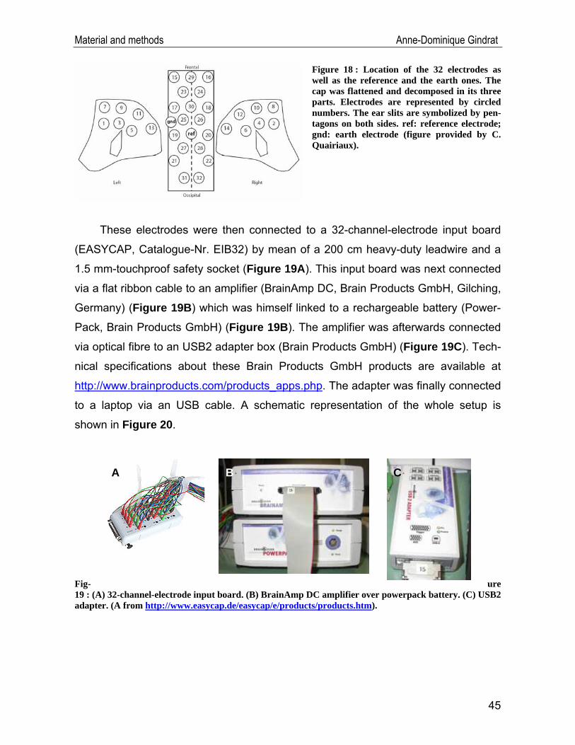
Material and methods Anne-Dominique Gindrat
Figure 18 : Location of the 32 electrodes as well as the reference and the earth ones. The cap was flattened and decomposed in its three parts. Electrodes are represented by circled numbers. The ear slits are symbolized by pen-tagons on both sides. ref: reference electrode; gnd: earth electrode (figure provided by C. Quairiaux).
These electrodes were then connected to a 32-channel-electrode input board
(EASYCAP, Catalogue-Nr. EIB32) by mean of a 200 cm heavy-duty leadwire and a
1.5 mm-touchproof safety socket (Figure 19A). This input board was next connected
via a flat ribbon cable to an amplifier (BrainAmp DC, Brain Products GmbH, Gilching,
Germany) (Figure 19B) which was himself linked to a rechargeable battery (Power-
Pack, Brain Products GmbH) (Figure 19B). The amplifier was afterwards connected
via optical fibre to an USB2 adapter box (Brain Products GmbH) (Figure 19C). Tech-
nical specifications about these Brain Products GmbH products are available at
http://www.brainproducts.com/products_apps.php. The adapter was finally connected
to a laptop via an USB cable. A schematic representation of the whole setup is
shown in Figure 20. Fig- ure 19 : (A) 32-channel-electrode input board. (B) BrainAmp DC amplifier over powerpack battery. (C) USB2 adapter. (A from http://www.easycap.de/easycap/e/products/products.htm).
A B A C A
A
45
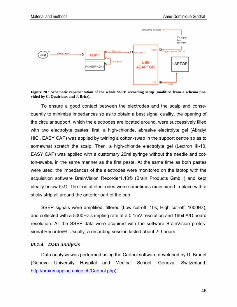
Material and methods Anne-Dominique Gindrat
Figure 20 : Schematic representation of the whole SSEP recording setup (modified from a schema pro-vided by C. Quairiaux and J. Britz).
To ensure a good contact between the electrodes and the scalp and conse-
quently to minimize impedances so as to obtain a best signal quality, the opening of
the circular support, which the electrodes are located around, were successively filled
with two electrolyte pastes: first, a high-chloride, abrasive electrolyte gel (Abralyt
HiCl, EASY CAP) was applied by twirling a cotton-swab in the support centre so as to
somewhat scratch the scalp. Then, a high-chloride electrolyte gel (Lectron III-10,
EASY CAP) was applied with a customary 20ml syringe without the needle and cot-
ton-swabs, in the same manner as the first paste. At the same time as both pastes
were used, the impedances of the electrodes were monitored on the laptop with the
acquisition software BrainVision Recorder1.10® (Brain Products GmbH) and kept
ideally below 5kΩ. The frontal electrodes were sometimes maintained in place with a
sticky strip all around the anterior part of the cap.
SSEP signals were amplified, filtered (Low cut-off: 10s; High cut-off: 1000Hz),
and collected with a 5000Hz sampling rate at a 0.1mV resolution and 16bit A/D board
resolution. All the SSEP data were acquired with the software BrainVision profes-
sional Recorder®. Usually, a recording session lasted about 2-3 hours.
III.1.4. Data analysis
Data analysis was performed using the Cartool software developed by D. Brunet
(Geneva University Hospital and Medical School, Geneva, Switzerland;
http://brainmapping.unige.ch/Cartool.php).
46
Material and methods Anne-Dominique Gindrat
The responses were filtered offline between 8Hz and 300Hz, a notch at 50Hz
was sometimes applied in order to eliminate the noise produced by surrounding elec-
trical installations, and the DC component (0Hz) was removed. The signals were re-
computed against the average reference. SSEPs were obtained by averaging be-
tween 75 and 600 stimulations, depending on the stimulation frequency and acquisi-
tion time. Channels which showed artefacts from electromagnetic noise or channels
which did not display any responses were excluded from the calculations. Moreover,
responses to each stimulus were checked offline to ensure that they were not con-
taminated by noise, in which case they were expelled. Data were baseline corrected,
using the 50ms pre-stimulus period. The responses were computed from 50ms be-
fore to 450ms after the stimulation onset, meaning that the analysis was performed
for 500ms peri-stimulus epochs. Positive responses were plotted upward.
When several recordings were obtained in the same conditions, grand averages
were performed between them so as to obtain averaged data available, as in the
case of right median nerve SSEPs obtained under 2.5% sevoflurane anaesthesia (n=
10 recordings). In the other cases, single recordings were considered.
SSEP data can be analysed in two different ways: according to the classical
method, some electrodes located over strategic positions are chosen and peaks are
studied in terms of latency and amplitude. In our study, we selected electrodes lo-
cated probably over the brain stem (e31 after stimulation on the right side, e32 after
stimulation on the left side), as well as electrodes showing the highest activity on the
contralateral cortex (e19 after right median nerve stimulation, e20 after left median
nerve stimulation and e33 after right or left tibial nerve stimulation) (Figure 21). e31
and e32 were selected because they registered initial negative activity in the brain
stem before the processing in the cortex. e19 and e20 were probably located over
the hand area of M1 and S1 as in a previous study of the laboratory (Gindrat, 2008;
Kaeser et al., 2006, 2007), where the responses are thought to be generated. e33 is
supposed to be located over the leg area of M1 and S1, near the midline. On e19,
e20 and e33, the main positive cortical peak was studied. Amplitudes and latencies
(from the stimulation delivery) of the SSEPs were determined using the cursor of the
47
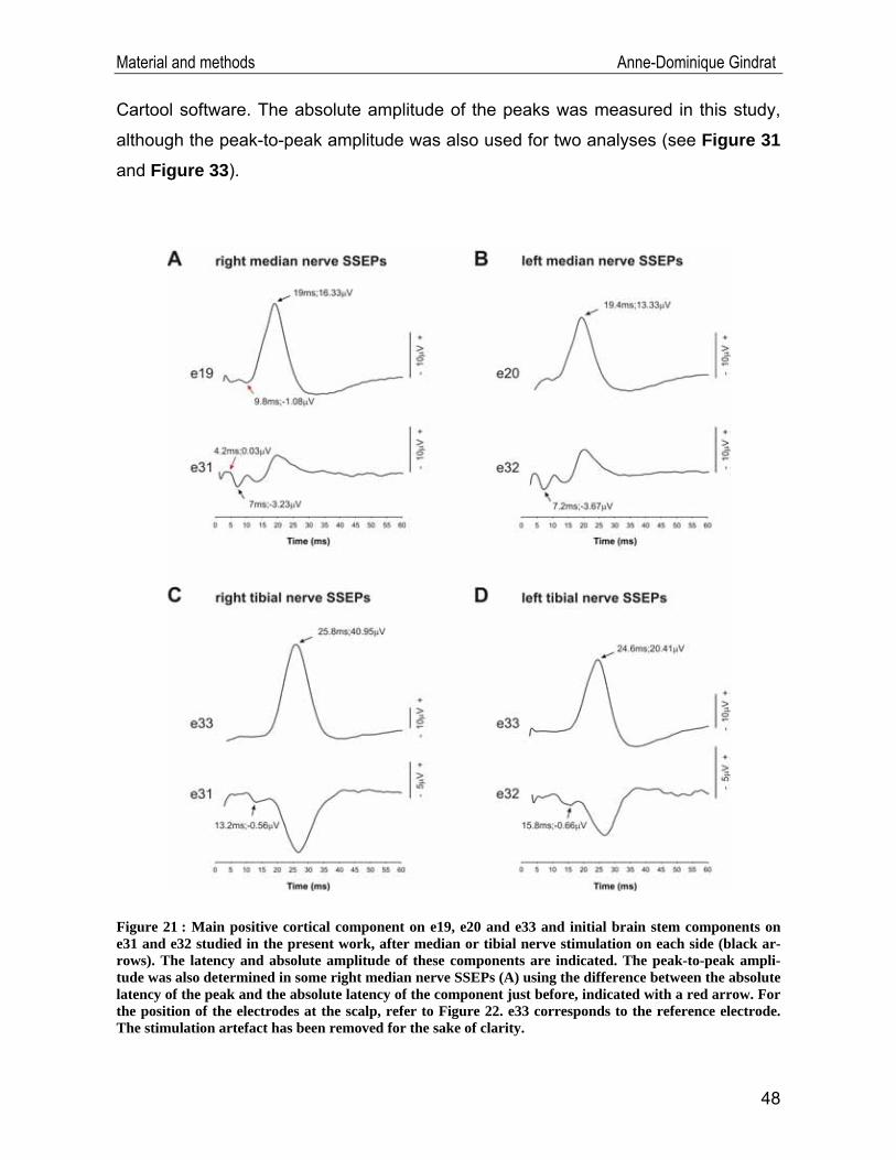
Material and methods Anne-Dominique Gindrat
Cartool software. The absolute amplitude of the peaks was measured in this study,
although the peak-to-peak amplitude was also used for two analyses (see Figure 31
and Figure 33).
Figure 21 : Main positive cortical component on e19, e20 and e33 and initial brain stem components on e31 and e32 studied in the present work, after median or tibial nerve stimulation on each side (black ar-rows). The latency and absolute amplitude of these components are indicated. The peak-to-peak ampli-tude was also determined in some right median nerve SSEPs (A) using the difference between the absolute latency of the peak and the absolute latency of the component just before, indicated with a red arrow. For the position of the electrodes at the scalp, refer to Figure 22. e33 corresponds to the reference electrode. The stimulation artefact has been removed for the sake of clarity.
48
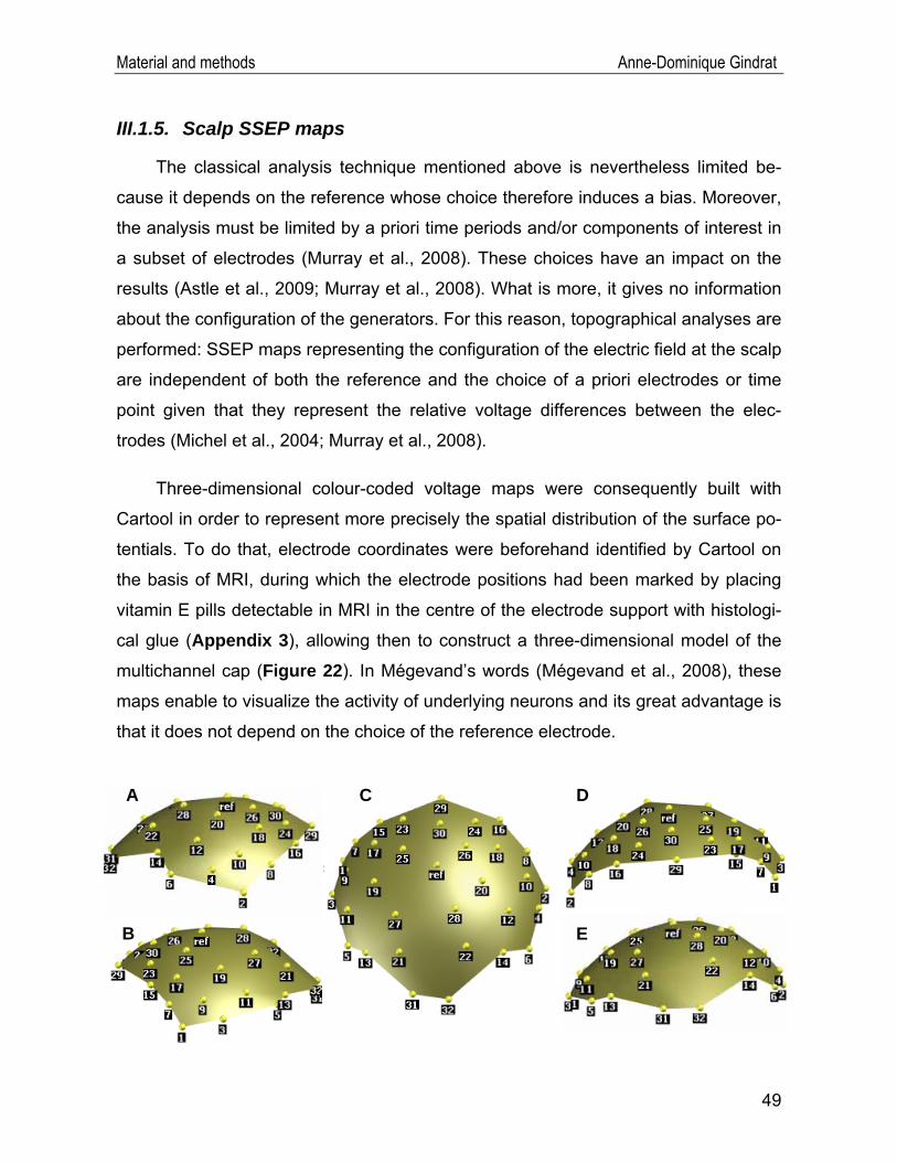
Material and methods Anne-Dominique Gindrat
III.1.5. Scalp SSEP maps
The classical analysis technique mentioned above is nevertheless limited be-
cause it depends on the reference whose choice therefore induces a bias. Moreover,
the analysis must be limited by a priori time periods and/or components of interest in
a subset of electrodes (Murray et al., 2008). These choices have an impact on the
results (Astle et al., 2009; Murray et al., 2008). What is more, it gives no information
about the configuration of the generators. For this reason, topographical analyses are
performed: SSEP maps representing the configuration of the electric field at the scalp
are independent of both the reference and the choice of a priori electrodes or time
point given that they represent the relative voltage differences between the elec-
trodes (Michel et al., 2004; Murray et al., 2008).
Three-dimensional colour-coded voltage maps were consequently built with
Cartool in order to represent more precisely the spatial distribution of the surface po-
tentials. To do that, electrode coordinates were beforehand identified by Cartool on
the basis of MRI, during which the electrode positions had been marked by placing
vitamin E pills detectable in MRI in the centre of the electrode support with histologi-
cal glue (Appendix 3), allowing then to construct a three-dimensional model of the
multichannel cap (Figure 22). In Mégevand’s words (Mégevand et al., 2008), these
maps enable to visualize the activity of underlying neurons and its great advantage is
that it does not depend on the choice of the reference electrode.
A
B
C D
E
49
Material and methods Anne-Dominique Gindrat
Figure 22 (previous page) : Three-dimensional model of the multichannel cap. (A) Lateral view from the right. (B) Lateral view from the left. (C) View from the top. (D) Frontal view. (E) Occipital view. Elec-trode 29 is rostralmost whereas electrodes 31 and 32 are caudalmost. The reference electrode (ref) is on the top and corresponds to e33. Even electrodes are on the right side and odd ones on the left side.
III.1.6. Identification of SSEP maps by cluster analysis
The brain electrical activity is composed of successive non-overlapping periods
with variable duration and variable intensity dynamics, corresponding each to a dif-
ferent relatively stable map topography and representing a different step of informa-
tion processing. Such periods are known as functional microstates (Pascual-Marqui
et al., 1995). To put it another way, the microstates represent the different SSEP
components that could explain the different steps in the brain activity evoked by a
stimulus. It is hypothesized that different map configurations result from different neu-
ral populations in the brain (Michel et al., 1999; Michel et al., 2001; Michel et al.,
2004; Pascual-Marqui et al., 1995). Therefore, it is interesting to segment or cluster
the SSEPs to determine the most important stable map topographies optimally sum-
marizing the data (Murray et al., 2008; Pascual-Marqui et al., 1995).
To this aim, we applied a clustering algorithm implemented in Cartool, called
Topographical Atomize and Agglomerate Hierarchical Clustering7 (T-AAHC). This
method is based on a hierarchical clustering. Segments shorter than 2ms (10TF)
were excluded and associated with the preceding or the following segment, depend-
ing on which they correlated better with. The numbers of segments was set to a
maximum of ten. This cluster analysis was computed on an interval ranging from
4.8ms post-stimulus to 60ms post-stimulus for median nerve SSEPs and from 8ms to
70ms post-stimulus for tibial nerve SSEPs. A cluster analysis provides several seg-
mentation results with variable number of maps to explain the whole data series.
Therefore, the Krzanowski-Lai criterion was applied to defining the optimal number of
maps and their individual duration, summarizing the activity with the lowest variability.
Finally, potential values were averaged during each segment obtained by clus-
tering at each electrode and interpolated with Delaunay triangulations for graphical
7 For further details about this method, see http://brainmapping.unige.ch/cartool/refguide/segmentation.htm
50
Material and methods Anne-Dominique Gindrat
representations of mean SSEP maps.
III.2. Behavioural tests8
In a lesional perspective, where it will be relevant to determine the recovery of
manual dexterity, namely the use of independent movements of the fingers, we have
begun to train the monkey to perform quantitative finger prehension tasks so as to
obtain pre-lesional baselines. During all these tests, the animal was sitting in a pri-
mate chair in Plexiglas®, with an opening on the top for the head and two independ-
ent sliding doors at the front, one for each arm. To this aim, the monkey was before-
hand habituated to sitting in this primate chair.
Then the animal was daily trained to perform the so-called modified Brinkman
board test. This behavioural task was designed to assess the precision grip (Napier,
1956), namely a series of fractionated finger movements allowing the precise opposi-
tion of the index and the thumb. It was initially described by Brinkman and Kuypers
(1973) and Brinkman (1984) and the protocol was then improved in the laboratory of
Prof. Rouiller (Liu et Rouiller, 1999; Rouiller et al., 1998; Schmidlin et al., 2005). This
modified version of the test requires the use of a rectangular board in green Per-
spex® (22cm long, 12cm wide) containing 25 vertically and 25 horizontally oriented
oval slots (15mm long, 8mm wide, 6mm deep), each filled with a small banana pellet
(about 4mm diameter). In practical terms, the monkey was sitting in its primate chair
and placed in front of the modified Brinkman board tilted with an angle of 40° in front
of the animal. The goal for the monkey was to retrieve the pellets from the slots by
introducing as a rule the distal phalange of the index and forming the precision grip
by opposing the thumb. This task allows to assess the manual dexterity resulting
from tactile, proprioceptive and visual inputs (Wyss, 2007). During each behavioural
session, tests were conducted separately with each hand and then with both hands
together. This exercise is more complex when grasping from the horizontal slots
given that an additional rotation of the wrist is required as compared to reaching from
the vertical slots (Freund et al., 2009). Each test session was videotaped (25
8 Short sequences of these tests are available on http://www.unifr.ch/neuro/rouiller/research/motorcontcadre.php
51
Material and methods Anne-Dominique Gindrat
frames/s) and simultaneously recorded with a webcam on a computer (15 frames/s),
allowing subsequently to establish the behavioural scores by counting the number of
pellets correctly retrieved from the slots and eaten during 30s, i.e. the score in 30s.
These analyses were performed by using the automatic analysis software Monkey-
Cam® and sometimes by experimenter’s viewing the webcam recording to confirm
the results. However, investigations in the laboratory showed that automatic analyses
with MonkeyCam® give similar results to those obtained by viewing the recording
and are therefore sufficient (data not shown). Statistical analyses (bilateral paired t-
test, confidence interval: 95%) were carried out with the software GraphPad Prism®.
In addition, the force of the arm of the monkey was unimanually tested with the
reach and grasp drawer task, derived and upgraded from a previously described ver-
sion (Kazennikov et al., 1994, 1998, 1999; Kermadi et al., 1997, 1998, 2000; Wannier
et al., 2002). The setup consists of a small drawer (5cm x 4.5cm x 3 cm) containing
inside a hollow which can be filled with a banana pellet. The drawer is placed be-
tween two sensors detecting the hand of the monkey during the gripping and pulling
phases. Moreover, there are sensors inside the hollow of the drawer, allowing to de-
tect the fingers of the monkey during the picking phase. The monkey was asked to
grip and pull the handle of the drawer placed in front of it so as to open this drawer
and retrieve with the same hand the banana pellet hidden inside. When the drawer is
pulled, it stays in the open position to allow the retrieval of the pellet. The resistance
of the drawer can be adjusted to different levels. This task allows to assess precisely
the gripping and pulling phases where the animal has to generate enough force to
open the drawer by holding firmly the handle. Moreover, the picking, which is hy-
pothesized to be disrupted after a lesion of the hand area of contralateral M1, is also
evaluated. Tests were carried out with each hand individually at increasing resis-
tances 0, 3, 5, 7 and finally 10, corresponding in Newtons to 0N, 1.35N, 2.8N, 5N and
9N respectively (static load force measures). A daily session consisted of several re-
trievals performed at each resistance, in order to obtain a bloc of a least 5 successive
corrects retrievals for each hand at each investigated resistance, except for the
forces 7 and 10 where only 2-3 successive correct retrievals were minimally required
in the first days given that this exercise was really difficult. These blocs of successive
52

Material and methods Anne-Dominique Gindrat
53
correct retrievals were further analysed. A trial usually lasted not longer than 2s and
the next trial was initiated after 2s-4s (up to 13s at resistance 10, due to the difficulty
of the exercise). A pause of a few minutes was provided between each resistance.
The result were recorded on a computer equipped with the software Spike 2® (Cam-
bridge Electronic Design) and later analysed with the Spike 2® and Matlab® soft-
wares. The quantitative parameters analysed were the grip force, the load force, the
picking time and the pulling time (average of five trials per day). Statistical tests (bi-
lateral paired t-test, confidence interval: 95%) were performed with the software
GraphPad Prism®.
Other manual dexterity tests were performed daily, i.e. the hidden Brinkman
board task and the rotative Brinkman board task but these results will not be pre-
sented here because they are beyond the scope of the present work.
Simultaneously, as the goal in the future is to perform SSEP recordings in an
awake monkey using the EEG cap, we took advantage of these dexterity tests to get
the animal used to wearing a cap at the scalp. A first model of the cap, without elec-
trodes, was used and placed at the scalp of the monkey for the behavioural tests.
All the tests were performed 2 to 5 days a week, usually late in the morning,
with a music background to mask distracting surrounding noises. A daily test session
typically lasted 60-70 minutes if all the four behavioural tests are considered. Note
that the monkey was not restricted in time to do these tasks, but it appeared that it
did them quite fast due to the motivation of getting additional rewards if the tests
were performed correctly. At the end of these behavioural tests, the animal received
its daily food ration (fruits, cereal). Behavioural tasks were not performed on the days
where SSEPs were recorded.
Results Anne-Dominique Gindrat
IV. Results
IV.1. SSEP data
All SSEPs were submitted to peak analyses, i.e. calculation of latency and ab-
solute amplitude of major components at selected electrodes, and in some cases to
topographic segmentation analyses at the whole brain level. Both these techniques
are complementary: the peak analysis gives information about differences in the
strength between two situations, while the topographical analysis illustrates changes
in the electrical field distribution (Astle, 2009).
IV.1.1. Example of a typical SSEP recording
Figure 23A shows a representative example of SSEPs evoked by electrical
right median nerve stimulation (0.5Hz, 1.74mA) at 2.5% sevoflurane (without any pre-
induction of the anaesthesia). In this example, scalp SSEP signals were filtered off-
line between 8Hz and 300Hz and averaged for 75 sweeps. A huge stimulation arte-
fact can be observed beginning about 3ms before the stimulus (stimulus: 0ms in the
x-axis) and lasting for about 4ms post-stimulus (grey rectangle). The pre-stimulation
artefact is probably due to an aliasing effect of the filtering process. Then, positive
and negative deflections on each isolated channel can be seen, corresponding to ac-
tivity supposed to be generated successively in the spinal cord, in the brain stem, in
subcortical region and finally, for the long-latency components, in the cerebral cortex.
Responses are plotted here as an example from 5ms pre-stimulation to 150ms post-
stimulation but as it can be seen, relevant evoked responses last about up to
60ms.This interval from the end of the artefact up to 60ms will be conserved in the
next parts of this work.
Figure 23B illustrates the signals recorded from two electrodes of interest, e31
and e19, which coordinates presumably correspond to the left brain stem and sen-
sorimotor cortex respectively, contralateral to the stimulation. In our peak analyses
we focused on two major components recorded at these electrodes: first, the initial
negative component on e31 that should reflect the arrival of the afferent volleys on
the brain stem peaking 7ms post-stimulus; then, the main positive cortical peak that
54
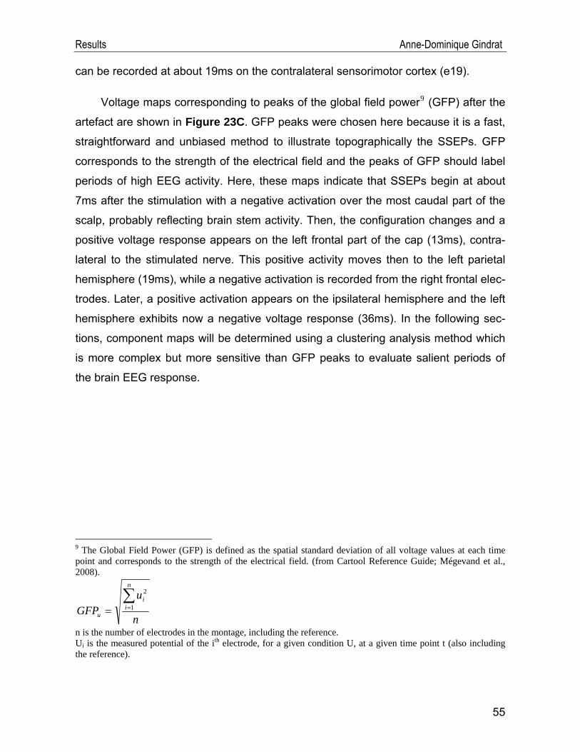
Results Anne-Dominique Gindrat
can be recorded at about 19ms on the contralateral sensorimotor cortex (e19).
Voltage maps corresponding to peaks of the global field power9 (GFP) after the
artefact are shown in Figure 23C. GFP peaks were chosen here because it is a fast,
straightforward and unbiased method to illustrate topographically the SSEPs. GFP
corresponds to the strength of the electrical field and the peaks of GFP should label
periods of high EEG activity. Here, these maps indicate that SSEPs begin at about
7ms after the stimulation with a negative activation over the most caudal part of the
scalp, probably reflecting brain stem activity. Then, the configuration changes and a
positive voltage response appears on the left frontal part of the cap (13ms), contra-
lateral to the stimulated nerve. This positive activity moves then to the left parietal
hemisphere (19ms), while a negative activation is recorded from the right frontal elec-
trodes. Later, a positive activation appears on the ipsilateral hemisphere and the left
hemisphere exhibits now a negative voltage response (36ms). In the following sec-
tions, component maps will be determined using a clustering analysis method which
is more complex but more sensitive than GFP peaks to evaluate salient periods of
the brain EEG response.
9 The Global Field Power (GFP) is defined as the spatial standard deviation of all voltage values at each time point and corresponds to the strength of the electrical field. (from Cartool Reference Guide; Mégevand et al., 2008).
n
uGFP
n
ii
u
∑== 1
2
n is the number of electrodes in the montage, including the reference. Ui is the measured potential of the ith electrode, for a given condition U, at a given time point t (also including the reference).
55
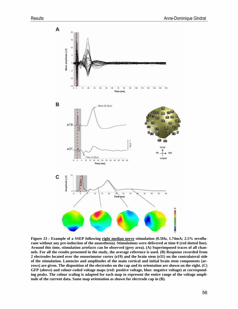
Results Anne-Dominique Gindrat
Figure 23 : Example of a SSEP following right median nerve stimulation (0.5Hz, 1.74mA; 2.5% sevoflu-rane without any pre-induction of the anaesthesia). Stimulations were delivered at time 0 (red dotted line). Around this time, stimulation artefacts can be observed (grey area). (A) Superimposed traces of all chan-nels. For all the results presented in the study, the average reference is used. (B) Response recorded from 2 electrodes located over the sensorimotor cortex (e19) and the brain stem (e31) on the contralateral side of the stimulation. Latencies and amplitudes of the main cortical and initial brain stem components (ar-rows) are given. The disposition of the electrodes on the cap and its orientation are shown on the right. (C) GFP (above) and colour-coded voltage maps (red: positive voltage, blue: negative voltage) at correspond-ing peaks. The colour scaling is adapted for each map to represent the entire range of the voltage ampli-tude of the current data. Same map orientation as shown for electrode cap in (B).
56
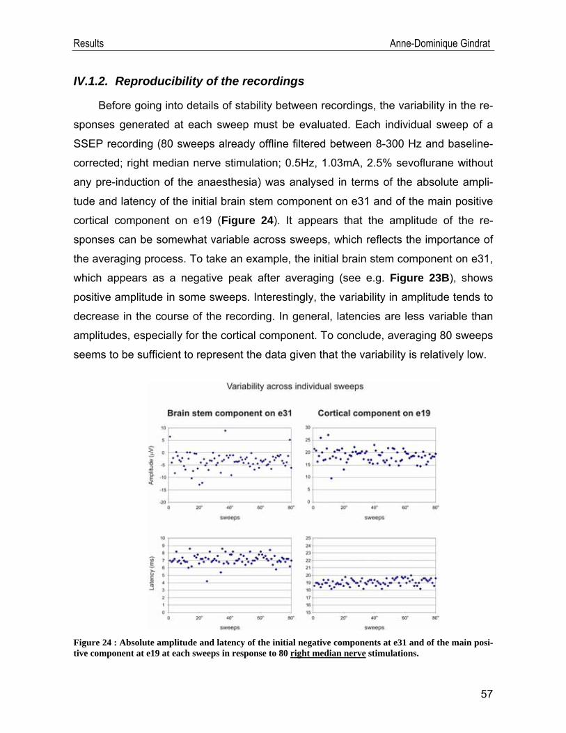
Results Anne-Dominique Gindrat
IV.1.2. Reproducibility of the recordings
Before going into details of stability between recordings, the variability in the re-
sponses generated at each sweep must be evaluated. Each individual sweep of a
SSEP recording (80 sweeps already offline filtered between 8-300 Hz and baseline-
corrected; right median nerve stimulation; 0.5Hz, 1.03mA, 2.5% sevoflurane without
any pre-induction of the anaesthesia) was analysed in terms of the absolute ampli-
tude and latency of the initial brain stem component on e31 and of the main positive
cortical component on e19 (Figure 24). It appears that the amplitude of the re-
sponses can be somewhat variable across sweeps, which reflects the importance of
the averaging process. To take an example, the initial brain stem component on e31,
which appears as a negative peak after averaging (see e.g. Figure 23B), shows
positive amplitude in some sweeps. Interestingly, the variability in amplitude tends to
decrease in the course of the recording. In general, latencies are less variable than
amplitudes, especially for the cortical component. To conclude, averaging 80 sweeps
seems to be sufficient to represent the data given that the variability is relatively low.
Figure 24 : Absolute amplitude and latency of the initial negative components at e31 and of the main posi-tive component at e19 at each sweeps in response to 80 right median nerve stimulations.
57
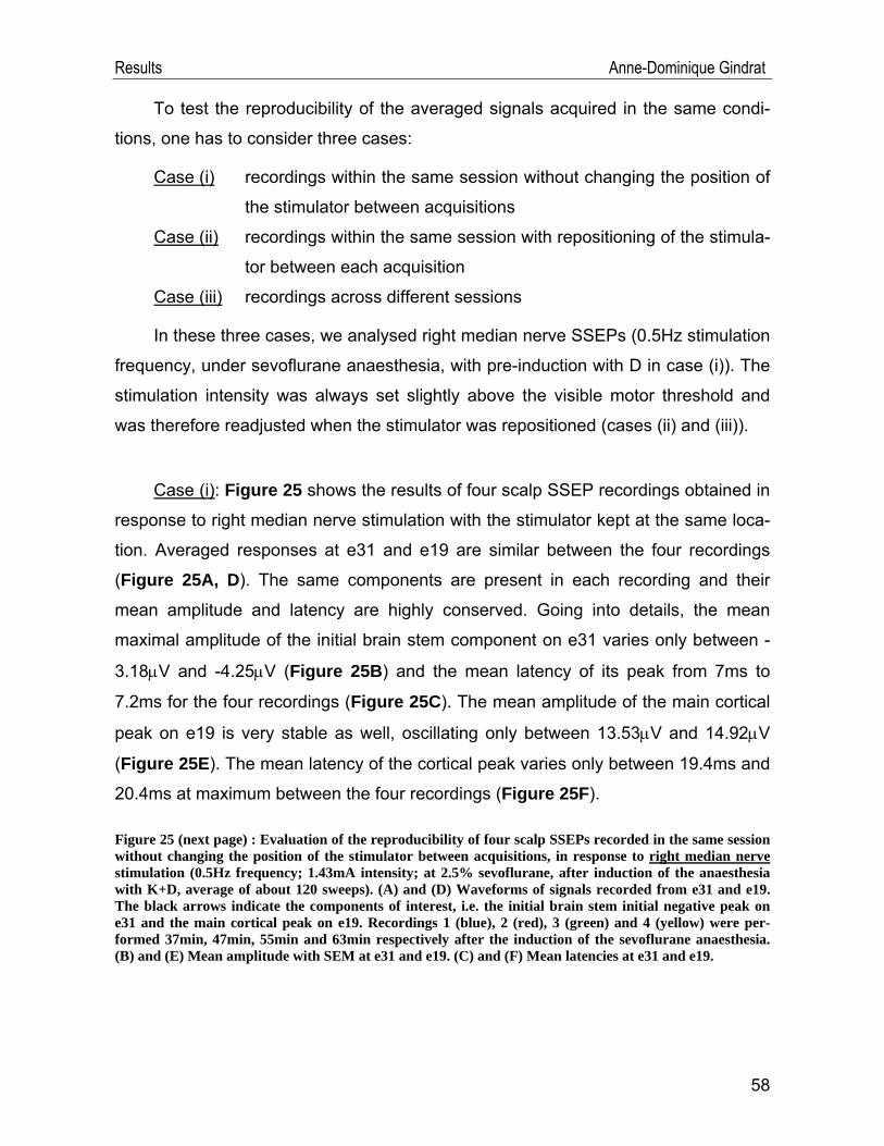
Results Anne-Dominique Gindrat
To test the reproducibility of the averaged signals acquired in the same condi-
tions, one has to consider three cases:
Case (i) recordings within the same session without changing the position of
the stimulator between acquisitions
Case (ii) recordings within the same session with repositioning of the stimula-
tor between each acquisition
Case (iii) recordings across different sessions
In these three cases, we analysed right median nerve SSEPs (0.5Hz stimulation
frequency, under sevoflurane anaesthesia, with pre-induction with D in case (i)). The
stimulation intensity was always set slightly above the visible motor threshold and
was therefore readjusted when the stimulator was repositioned (cases (ii) and (iii)).
Case (i): Figure 25 shows the results of four scalp SSEP recordings obtained in
response to right median nerve stimulation with the stimulator kept at the same loca-
tion. Averaged responses at e31 and e19 are similar between the four recordings
(Figure 25A, D). The same components are present in each recording and their
mean amplitude and latency are highly conserved. Going into details, the mean
maximal amplitude of the initial brain stem component on e31 varies only between -
3.18μV and -4.25μV (Figure 25B) and the mean latency of its peak from 7ms to
7.2ms for the four recordings (Figure 25C). The mean amplitude of the main cortical
peak on e19 is very stable as well, oscillating only between 13.53μV and 14.92μV
(Figure 25E). The mean latency of the cortical peak varies only between 19.4ms and
20.4ms at maximum between the four recordings (Figure 25F).
Figure 25 (next page) : Evaluation of the reproducibility of four scalp SSEPs recorded in the same session without changing the position of the stimulator between acquisitions, in response to right median nerve stimulation (0.5Hz frequency; 1.43mA intensity; at 2.5% sevoflurane, after induction of the anaesthesia with K+D, average of about 120 sweeps). (A) and (D) Waveforms of signals recorded from e31 and e19. The black arrows indicate the components of interest, i.e. the initial brain stem initial negative peak on e31 and the main cortical peak on e19. Recordings 1 (blue), 2 (red), 3 (green) and 4 (yellow) were per-formed 37min, 47min, 55min and 63min respectively after the induction of the sevoflurane anaesthesia. (B) and (E) Mean amplitude with SEM at e31 and e19. (C) and (F) Mean latencies at e31 and e19.
58
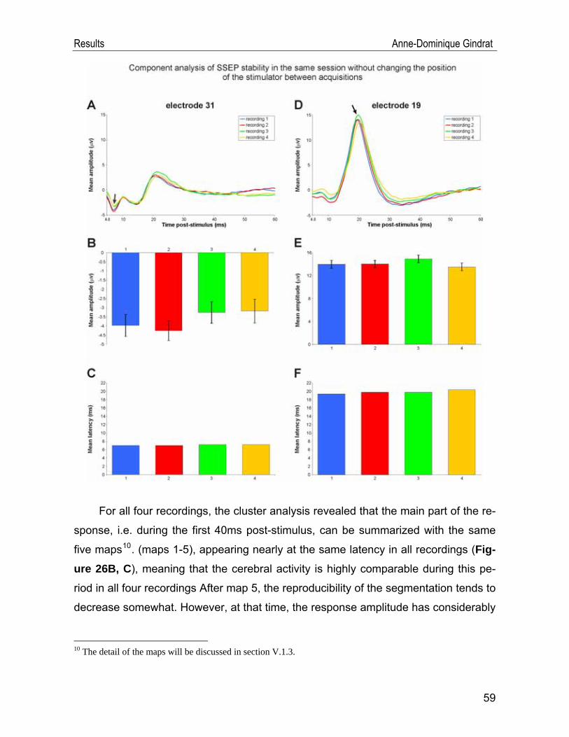
Results Anne-Dominique Gindrat
For all four recordings, the cluster analysis revealed that the main part of the re-
sponse, i.e. during the first 40ms post-stimulus, can be summarized with the same
five maps10. (maps 1-5), appearing nearly at the same latency in all recordings (Fig-ure 26B, C), meaning that the cerebral activity is highly comparable during this pe-
riod in all four recordings After map 5, the reproducibility of the segmentation tends to
decrease somewhat. However, at that time, the response amplitude has considerably
10 The detail of the maps will be discussed in section V.1.3.
59
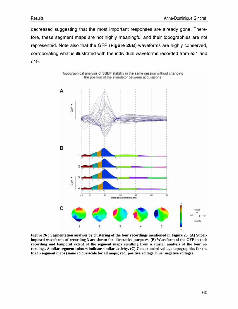
Results Anne-Dominique Gindrat
decreased suggesting that the most important responses are already gone. There-
fore, these segment maps are not highly meaningful and their topographies are not
represented. Note also that the GFP (Figure 26B) waveforms are highly conserved,
corroborating what is illustrated with the individual waveforms recorded from e31 and
e19.
Figure 26 : Segmentation analysis by clustering of the four recordings mentioned in Figure 25. (A) Super-imposed waveforms of recording 3 are shown for illustrative purposes. (B) Waveform of the GFP in each recording and temporal extent of the segment maps resulting from a cluster analysis of the four re-cordings. Similar segment colours indicate similar activity. (C) Colour-coded voltage topographies for the first 5 segment maps (same colour-scale for all maps; red: positive voltage, blue: negative voltage).
60
Results Anne-Dominique Gindrat
In sum, SSEPs obtained in the same session without moving the stimula-tor between acquisitions are very reproducible between each other, especially for the first 40ms after the stimulation, where the most important activity is present (Figure 28A).
Case (ii): Figure 27 depicts the stability of four recordings in response to right
median nerve stimulations, obtained in the same session with repositioning of the
stimulator between each acquisition. Here again, the morphology of the signals re-
corded over the brain stem from e31 and over the contralateral sensorimotor cortex
from e19 is well conserved (Figure 27A, D). The initial brain stem peak on e31 re-
mains highly stable in the four recordings: the mean amplitude varies only from -
3.07μV to -3.61 μV (Figure 27B) and the mean latency is comprised between 6.8ms
and 7.4ms (Figure 27C). The mean amplitude of the main cortical peak on e19 var-
ies from 16.33μV to 20.09μV (Figure 27E) and its mean latency from 18.4ms to
20ms during the four recordings (Figure 27F).
Figure 27 (next page) : Evaluation of the reproducibility of four scalp SSEPs recorded in the same session by repositioning the stimulator between each acquisition, in response to right median nerve stimulation (0.5Hz frequency; stimulation intensity: 1.99mA, 1.03mA, 1.74mA, 1.99mA respectively in recordings 1-4; at 2.5% sevoflurane, without any pre-induction of the anaesthesia; average of about 75 sweeps). (A) and (D) Same conventions as in Figure 25. Recordings 1 (blue), 2 (red), 3 (green) and 4 (yellow) were per-formed 76min, 81min, 90min and 100min respectively after the induction of the sevoflurane anaesthesia. (B, C, E, F) Same conventions as in Figure 25.
61
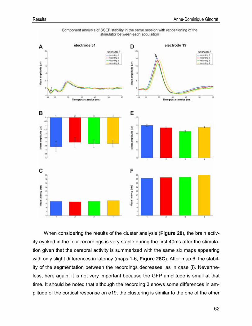
Results Anne-Dominique Gindrat
When considering the results of the cluster analysis (Figure 28), the brain activ-
ity evoked in the four recordings is very stable during the first 40ms after the stimula-
tion given that the cerebral activity is summarized with the same six maps appearing
with only slight differences in latency (maps 1-6, Figure 28C). After map 6, the stabil-
ity of the segmentation between the recordings decreases, as in case (i). Neverthe-
less, here again, it is not very important because the GFP amplitude is small at that
time. It should be noted that although the recording 3 shows some differences in am-
plitude of the cortical response on e19, the clustering is similar to the one of the other
62
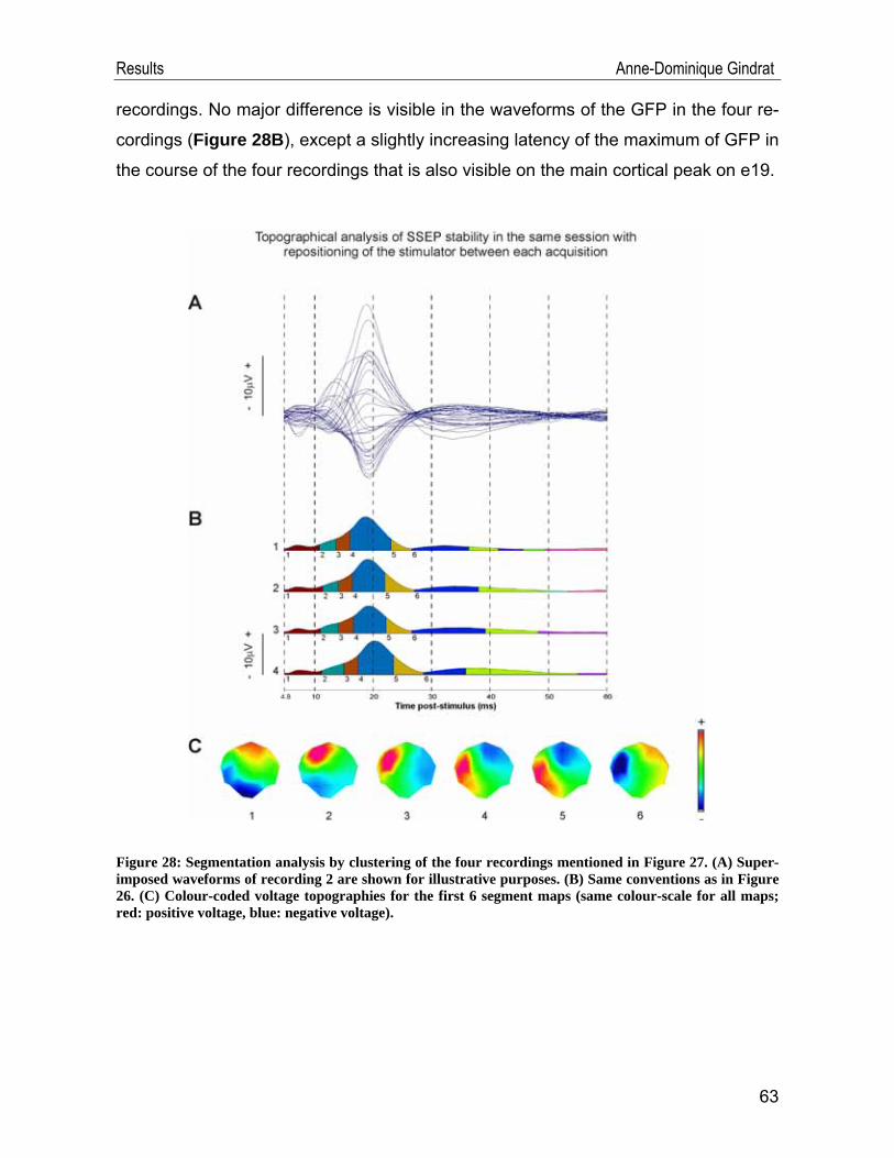
Results Anne-Dominique Gindrat
recordings. No major difference is visible in the waveforms of the GFP in the four re-
cordings (Figure 28B), except a slightly increasing latency of the maximum of GFP in
the course of the four recordings that is also visible on the main cortical peak on e19.
Figure 28: Segmentation analysis by clustering of the four recordings mentioned in Figure 27. (A) Super-imposed waveforms of recording 2 are shown for illustrative purposes. (B) Same conventions as in Figure 26. (C) Colour-coded voltage topographies for the first 6 segment maps (same colour-scale for all maps; red: positive voltage, blue: negative voltage).
63
Results Anne-Dominique Gindrat
To sum up, despite the fact that responses on e19 are more variable than when the stimulator was kept at the same place, the SSEP topography is very well conserved, even when the stimulator is repositioned between each re-cording.
Case (iii): As SSEPs were shown to be well reproducible within the same ses-
sion under sevoflurane anaesthesia (Figures 27 and 28), one recording per session
was selected to test the stability of right median nerve SSEPs across five different
sessions under sevoflurane anaesthesia (Figure 29).
In this case again, the same components are present in each recording session
on e31 and e19 (Figure 29A, D) but with more or less important differences in ampli-
tude and latency. The initial brain stem peak on e31 is very stable across the re-
cording sessions: the mean amplitude varies only from -3.07μV to -4.11μV across the
five sessions (Figure 29B) and the mean latency is comprised between 6.8ms and
7.6ms (Figure 29C). On the other hand, the mean amplitudes of the main cortical
peak on e19 are more variable, from 9.21μV to 18.65μV (Figure 29E). But if the first
session is excluded (9.21μV amplitude), the mean amplitudes in session 2-5 are
much more stable, comprised between 14.97μV and 18.7μV, and recordings 2 and 3
on e19 seem to be highly conserved, in amplitude as well as in latency. The mean
latency of the cortical peak on e19 is very stable in the first three recording sessions
(18.8ms-19ms) (Figure 29F). In the last two sessions, the latency increases at
21.6ms and 22ms, respectively.
Figure 29 (next page) : Evaluation of the reproducibility of five scalp SSEPs recorded across five different sessions, in response to right median nerve stimulation (0.5Hz frequency; stimulation intensity: 2.7mA, 4.0mA, 1.03mA, 2.5mA, 1.37mA respectively in recordings 1-5; at 2.5% sevoflurane, without any pre-induction of the anaesthesia; average of 67-117 sweeps). (A) and (D) Same conventions as in Figure 25. The recordings 1 (dark blue), 2 (red), 3 (green), 4 (yellow) and 5 (light blue) were performed on the 10.08.2009, 19.08.2009, 02.10.2009, 24.11.2009 and 03.12.2009. (B, C, E, F) Same conventions as in Figure 25.
64
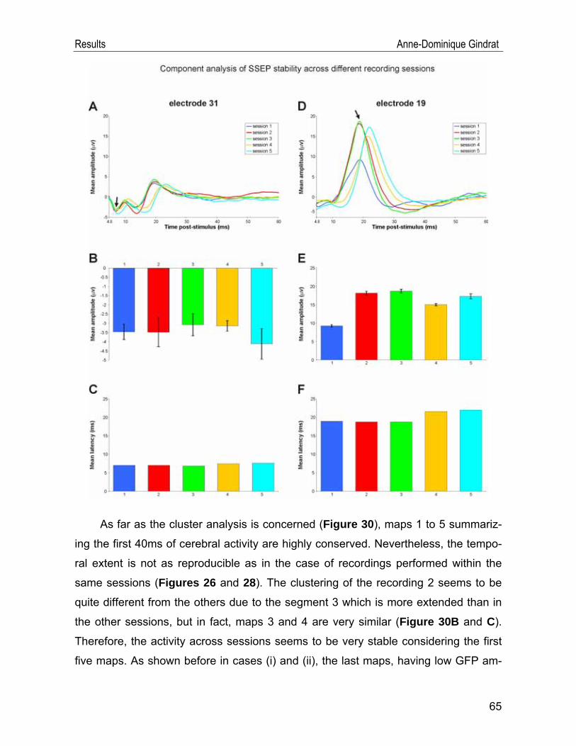
Results Anne-Dominique Gindrat
As far as the cluster analysis is concerned (Figure 30), maps 1 to 5 summariz-
ing the first 40ms of cerebral activity are highly conserved. Nevertheless, the tempo-
ral extent is not as reproducible as in the case of recordings performed within the
same sessions (Figures 26 and 28). The clustering of the recording 2 seems to be
quite different from the others due to the segment 3 which is more extended than in
the other sessions, but in fact, maps 3 and 4 are very similar (Figure 30B and C).
Therefore, the activity across sessions seems to be very stable considering the first
five maps. As shown before in cases (i) and (ii), the last maps, having low GFP am-
65
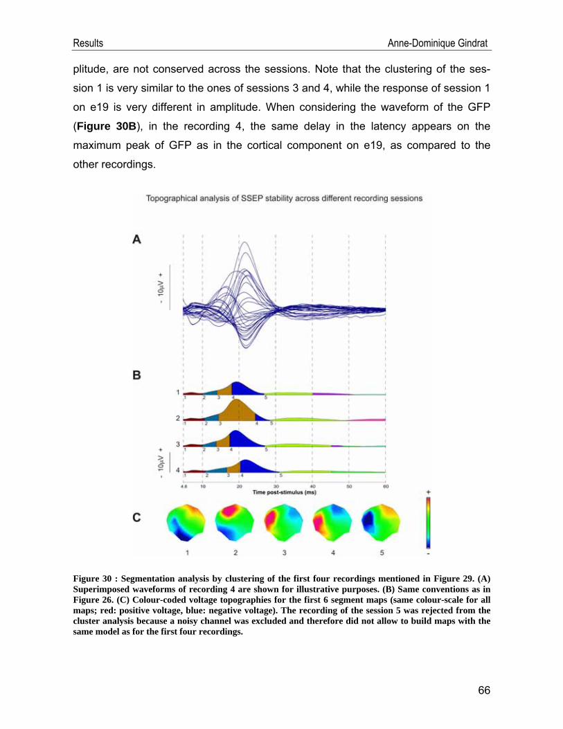
Results Anne-Dominique Gindrat
plitude, are not conserved across the sessions. Note that the clustering of the ses-
sion 1 is very similar to the ones of sessions 3 and 4, while the response of session 1
on e19 is very different in amplitude. When considering the waveform of the GFP
(Figure 30B), in the recording 4, the same delay in the latency appears on the
maximum peak of GFP as in the cortical component on e19, as compared to the
other recordings.
Figure 30 : Segmentation analysis by clustering of the first four recordings mentioned in Figure 29. (A) Superimposed waveforms of recording 4 are shown for illustrative purposes. (B) Same conventions as in Figure 26. (C) Colour-coded voltage topographies for the first 6 segment maps (same colour-scale for all maps; red: positive voltage, blue: negative voltage). The recording of the session 5 was rejected from the cluster analysis because a noisy channel was excluded and therefore did not allow to build maps with the same model as for the first four recordings.
66
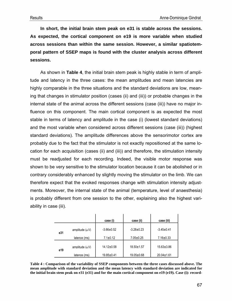
Results Anne-Dominique Gindrat
In short, the initial brain stem peak on e31 is stable across the sessions. As expected, the cortical component on e19 is more variable when studied across sessions than within the same session. However, a similar spatiotem-poral pattern of SSEP maps is found with the cluster analysis across different sessions.
As shown in Table 4, the initial brain stem peak is highly stable in term of ampli-
tude and latency in the three cases: the mean amplitudes and mean latencies are
highly comparable in the three situations and the standard deviations are low, mean-
ing that changes in stimulator position (cases (ii) and (iii)) or probable changes in the
internal state of the animal across the different sessions (case (iii)) have no major in-
fluence on this component. The main cortical component is as expected the most
stable in terms of latency and amplitude in the case (i) (lowest standard deviations)
and the most variable when considered across different sessions (case (iii)) (highest
standard deviations). The amplitude differences above the sensorimotor cortex are
probably due to the fact that the stimulator is not exactly repositioned at the same lo-
cation for each acquisition (cases (ii) and (iii)) and therefore, the stimulation intensity
must be readjusted for each recording. Indeed, the visible motor response was
shown to be very sensitive to the stimulator location because it can be abolished or in
contrary considerably enhanced by slightly moving the stimulator on the limb. We can
therefore expect that the evoked responses change with stimulation intensity adjust-
ments. Moreover, the internal state of the animal (temperature, level of anaesthesia)
is probably different from one session to the other, explaining also the highest vari-
ability in case (iii).
case (i) case (ii) case (iii)
e31 amplitude (μV) -3.66±0.52 -3.28±0.23 -3.45±0.41
latence (ms) 7.1±0.12 7.05±0.25 7.16±0.33
e19 amplitude (μV) 14.12±0.58 18.50±1.57 15.63±3.86
latence (ms) 19.85±0.41 19.05±0.68 20.04±1.61
Table 4 : Comparison of the variability of SSEP components between the three cases discussed above. The mean amplitude with standard deviation and the mean latency with standard deviation are indicated for the initial brain stem peak on e31 (e31) and for the main cortical component on e19 (e19). Case (i): record-
67
Results Anne-Dominique Gindrat
ings within the same session without changing the position of the stimulator between acquisitions; case (ii): recordings within the same session with repositioning of the stimulator between each acquisition; case (iii): recordings across different sessions.
Although there is some variability in amplitude and latency, the SSEP maps are
very similar across the three cases, as expected, given that the recording conditions
are nearly similar across the three cases. In case (ii) however, the segmentation
gives 6 maps for the first 40ms post-stimulus activity (Figure 28), whereas this period
was summarized with only 5 maps in cases (i) and (iii). But, when going into details, it
appears that maps 4 and 5 in case (ii) are in fact highly similar and correspond to
map 4 in cases (i) and (iii).
Because the onset of the components is not always exactly at 0μV, we repeated
the same analysis of SSEP reproducibility across the sessions (case (iii)) by measur-
ing the peak-to-peak amplitude (Figure 31) instead of the absolute amplitude of the
peaks. On e31, the mean amplitude of the initial negative component varies now
from -3.03μV to -4.07μV, a similar range than with the absolute amplitude measure
(from -3.07μV to -4.11μV). This operation has no major effect on the amplitude of the
main cortical peak on e19 either, with only a small increase in amplitude of 1.17μV to
2.48μV maximum.
Figure 31 (next page) : Comparison of the measure of the absolute amplitude and the peak-to-peak ampli-tude to evaluate the reproducibility of scalp SSEPs across the recording sessions (case iii), in response to right median nerve stimulation (see Figure 29 for more detail). (A) and (D) Waveforms of signals recorded from e31 and e19. The black arrows indicate the components of interest. The red arrows point to the onset of the component of interest, used to calculate the peak-to peak amplitude. (B) and (D) Absolute mean amplitude with SEM (dark green) and peak-to-peak mean amplitude (light green) of the initial brain stem peak on e31 and of the main cortical peak on e19.
68
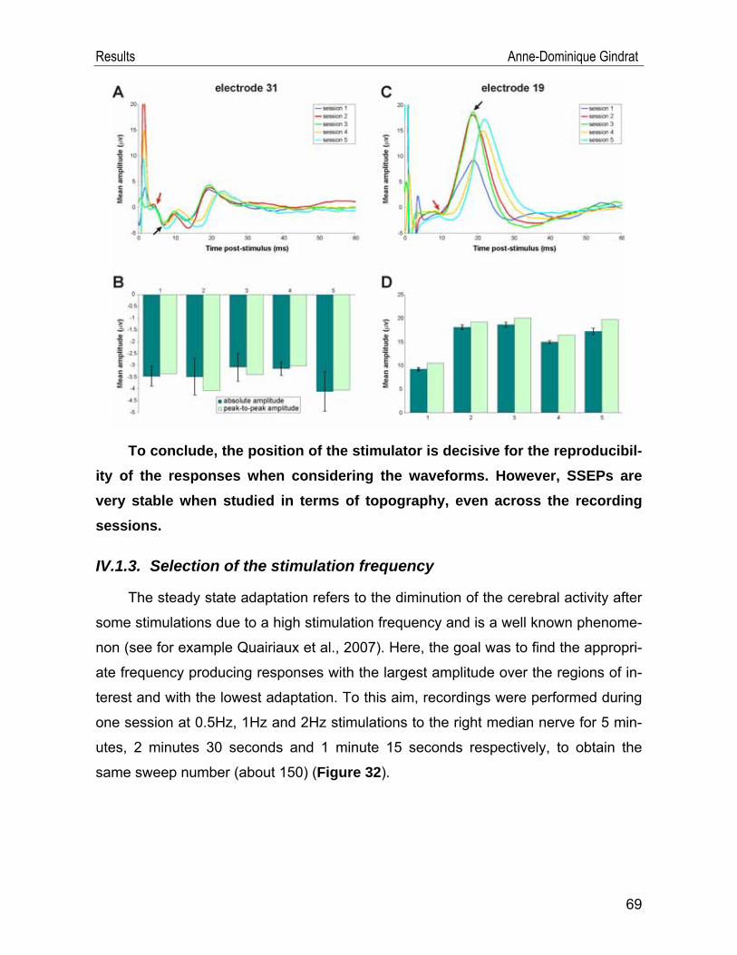
Results Anne-Dominique Gindrat
To conclude, the position of the stimulator is decisive for the reproducibil-ity of the responses when considering the waveforms. However, SSEPs are very stable when studied in terms of topography, even across the recording sessions.
IV.1.3. Selection of the stimulation frequency
The steady state adaptation refers to the diminution of the cerebral activity after
some stimulations due to a high stimulation frequency and is a well known phenome-
non (see for example Quairiaux et al., 2007). Here, the goal was to find the appropri-
ate frequency producing responses with the largest amplitude over the regions of in-
terest and with the lowest adaptation. To this aim, recordings were performed during
one session at 0.5Hz, 1Hz and 2Hz stimulations to the right median nerve for 5 min-
utes, 2 minutes 30 seconds and 1 minute 15 seconds respectively, to obtain the
same sweep number (about 150) (Figure 32).
69
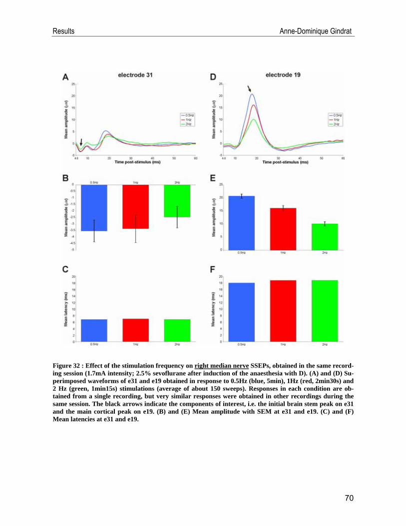
Results Anne-Dominique Gindrat
Figure 32 : Effect of the stimulation frequency on right median nerve SSEPs, obtained in the same record-ing session (1.7mA intensity; 2.5% sevoflurane after induction of the anaesthesia with D). (A) and (D) Su-perimposed waveforms of e31 and e19 obtained in response to 0.5Hz (blue, 5min), 1Hz (red, 2min30s) and 2 Hz (green, 1min15s) stimulations (average of about 150 sweeps). Responses in each condition are ob-tained from a single recording, but very similar responses were obtained in other recordings during the same session. The black arrows indicate the components of interest, i.e. the initial brain stem peak on e31 and the main cortical peak on e19. (B) and (E) Mean amplitude with SEM at e31 and e19. (C) and (F) Mean latencies at e31 and e19.
70

Results Anne-Dominique Gindrat
Signals obtained on the contralateral hemisphere on e31 and e19 are very simi-
lar in morphology in the three frequency conditions (Figure 32A, D). The amplitude
of the initial brain stem peak on e31 decreases only slightly as the repetition rate in-
creases (from -3.53μV to -2.47μV) (Figure 32B) and the latency changes of this
component are negligible (from 6.8ms to 7ms) (Figure32). On the other hand, impor-
tant changes in the amplitude of the cortical peak are visible on e19 (Figure 32E):
the higher the stimulation frequency is, the smaller the amplitudes of the evoked res-
ponses are (20.72μV vs 16.14μV vs 10.11μV). However, the latency of this cortical
peak at 1Hz and 2Hz stimulations is only slightly delayed, as compared to 0.5Hz sti-
mulation (18.8ms vs 18ms) (Figure 32F).
To evaluate the steady-state adaptation, the initial brain stem component on
e31 and the cortical peak on e19 were studied in terms of peak-to-peak amplitude
and latency on 60 individual sweeps already filtered and baseline-corrected obtained
at 0.5Hz, 1Hz and 2Hz (Figure 33A, B). Here, the peak-to-peak amplitude is used
although the data are already baseline-corrected, because the absolute amplitude
measure does not provide a trend as obvious as it appears with the peak-to-peak
measure. The initial brain stem component is very stable in amplitude and in latency
in the course of the first 60 sweeps at 0.5Hz (on average -4.02μV, 7.2ms), 1Hz (on
average -3.85μV, 7.4ms) as well as at 2Hz (on average -3.66μV, 7.2ms) (Figure
33A). Moreover, the differences in amplitude and latency in sweeps between the
three tested frequencies are minor, as already concluded with the averaged res-
ponses in Figure 32B and C. As far as the cortical peak on e19 is concerned (Figure 33B), there is much more variability in sweep amplitude. Moreover, a decrease in the
amplitude of the responses is visible in the first 30 sweeps obtained at 1Hz and 2Hz
repetition rate, Then the amplitudes become more stable (on average 16.86μV at
1Hz and 12.53μV at 2Hz). This decrease in the amplitude of the sweeps is surpri-
singly more evident at 1Hz than at 2Hz. On the other hand, no clear decrease in am-
plitude can be seen in sweeps obtained at 0.5Hz (on average 23.80μV). It is interest-
ing to note that despite the amplitude falls, the latency of the cortical peak on e19
remains stable in first 60 sweeps at the three tested frequencies (on average 18.3ms
71
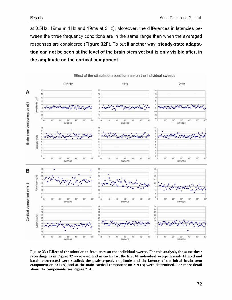
Results Anne-Dominique Gindrat
at 0.5Hz, 19ms at 1Hz and 19ms at 2Hz). Moreover, the differences in latencies be-
tween the three frequency conditions are in the same range than when the averaged
responses are considered (Figure 32F). To put it another way, steady-state adapta-tion can not be seen at the level of the brain stem yet but is only visible after, in the amplitude on the cortical component.
Figure 33 : Effect of the stimulation frequency on the individual sweeps. For this analysis, the same three recordings as in Figure 32 were used and in each case, the first 60 individual sweeps already filtered and baseline-corrected were studied: the peak-to-peak amplitude and the latency of the initial brain stem component on e31 (A) and of the main cortical component on e19 (B) were determined. For more detail about the components, see Figure 21A.
72
Results Anne-Dominique Gindrat
As the amplitude of the cortical signals obtained in response to 0.5Hz stimula-
tion was higher than with stimulations at 1Hz or 2Hz and as there was no obvious
adaptation at that frequency, we decided to keep this parameter of 0.5Hz for the following recording sessions.
In principle, recordings at 0.5Hz should be performed during a period twice or
four time as long as at 1Hz, respectively 2Hz to obtain the same sweep number. This
creates a trade-off between avoiding adaptation due to a high stimulation frequency
and having quite small acquisition periods. Consequently, we tried to determine the
number of sweeps required to obtain a representative response. To do that, right
median nerve SSEPs acquired at 0.5Hz during 5 minutes were averaged for all the
accepted sweeps (n= about 150) or using only the first half of them (n= about 75),
corresponding to a recording of about 2 minutes 30s: it appears that the waveforms
are very well conserved between both conditions (Figure 34). Although the SSEP
amplitude can sometimes be slightly smaller in a 2 minutes 30s acquisition than in a
5min one, these changes are minor. Therefore, averaging SSEPs for 75 sweeps (acquisition during 2 minutes 30s at 0.5Hz) is sufficient, as far as responses are not too much contaminated by noise. In such a case, more sweeps are needed.
73

Results Anne-Dominique Gindrat
- 10
μV +
Figure 34 : Effect of the acquired sweep number after 0.5Hz right median nerve stimulation (1.7mA in-tensity, 2.5% sevoflurane after induction of the anaesthesia with D). The same recording was averaged for 5min (black) and for the first 2min30s (red). All channels are shown. e33 corresponds to the reference electrode. Interval: from 4.8ms to 60 ms post-stimulus.
IV.1.4. Selection of the stimulation intensity
A recording session was specially devoted to evaluating the effect of the stimu-
lation intensity on the SSEPs. We tested stimulation intensities from 1.0mA to
4.25mA (interval of 0.25mA) on the right median nerve, the stimulator kept at the
same location for all acquisitions. The motor threshold was observed at 3.25mA (light
contraction of muscles at the basis of the thumb).
A careful analysis of the waveform recorded from e31 and e19 shows that the
general morphology of the responses is conserved from 4.25mA down to 1.5mA
stimulation intensities (Figure 35A, D). Then, at 1.25mA, it becomes more difficult to
distinguish the initial brain stem component on e31 and the components are no
longer visible at 1.0mA on both electrodes.
The peak amplitude of the initial brain stem component is quite constant from
4.25mA to 3.5mA (between -3.40μV and -3.95μV) (Figure 35B). Then, if signals ob-
74
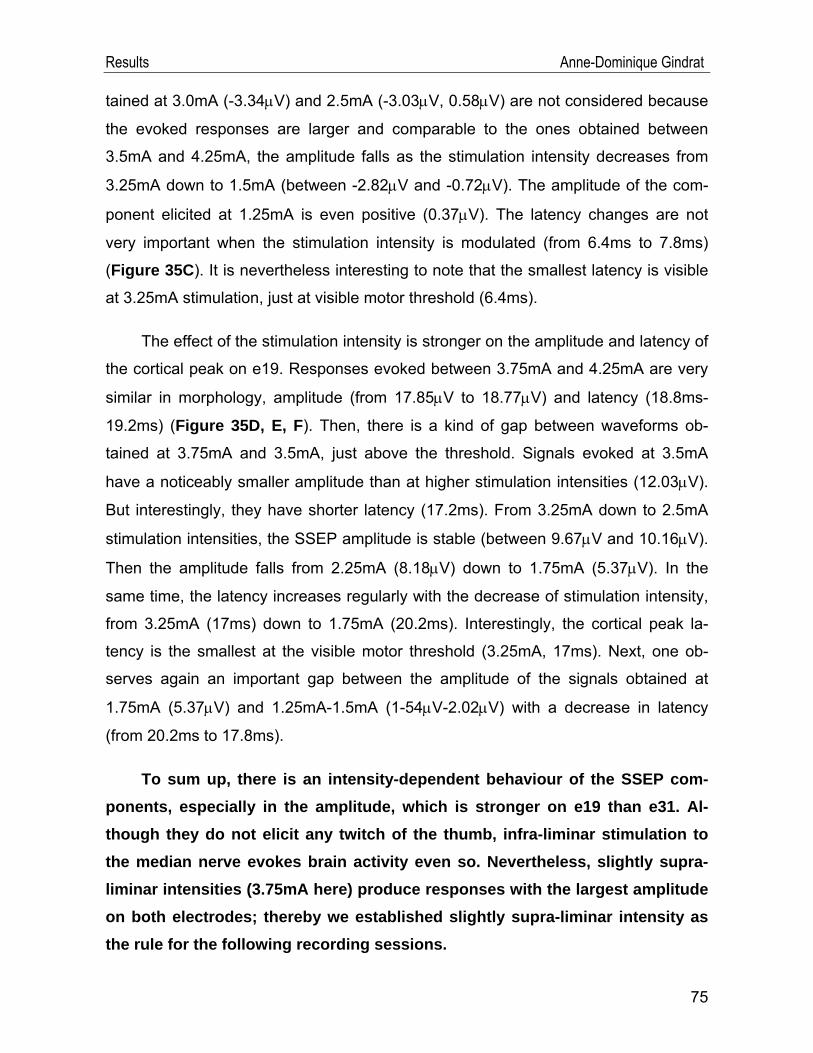
Results Anne-Dominique Gindrat
tained at 3.0mA (-3.34μV) and 2.5mA (-3.03μV, 0.58μV) are not considered because
the evoked responses are larger and comparable to the ones obtained between
3.5mA and 4.25mA, the amplitude falls as the stimulation intensity decreases from
3.25mA down to 1.5mA (between -2.82μV and -0.72μV). The amplitude of the com-
ponent elicited at 1.25mA is even positive (0.37μV). The latency changes are not
very important when the stimulation intensity is modulated (from 6.4ms to 7.8ms)
(Figure 35C). It is nevertheless interesting to note that the smallest latency is visible
at 3.25mA stimulation, just at visible motor threshold (6.4ms).
The effect of the stimulation intensity is stronger on the amplitude and latency of
the cortical peak on e19. Responses evoked between 3.75mA and 4.25mA are very
similar in morphology, amplitude (from 17.85μV to 18.77μV) and latency (18.8ms-
19.2ms) (Figure 35D, E, F). Then, there is a kind of gap between waveforms ob-
tained at 3.75mA and 3.5mA, just above the threshold. Signals evoked at 3.5mA
have a noticeably smaller amplitude than at higher stimulation intensities (12.03μV).
But interestingly, they have shorter latency (17.2ms). From 3.25mA down to 2.5mA
stimulation intensities, the SSEP amplitude is stable (between 9.67μV and 10.16μV).
Then the amplitude falls from 2.25mA (8.18μV) down to 1.75mA (5.37μV). In the
same time, the latency increases regularly with the decrease of stimulation intensity,
from 3.25mA (17ms) down to 1.75mA (20.2ms). Interestingly, the cortical peak la-
tency is the smallest at the visible motor threshold (3.25mA, 17ms). Next, one ob-
serves again an important gap between the amplitude of the signals obtained at
1.75mA (5.37μV) and 1.25mA-1.5mA (1-54μV-2.02μV) with a decrease in latency
(from 20.2ms to 17.8ms).
To sum up, there is an intensity-dependent behaviour of the SSEP com-ponents, especially in the amplitude, which is stronger on e19 than e31. Al-though they do not elicit any twitch of the thumb, infra-liminar stimulation to the median nerve evokes brain activity even so. Nevertheless, slightly supra-liminar intensities (3.75mA here) produce responses with the largest amplitude on both electrodes; thereby we established slightly supra-liminar intensity as the rule for the following recording sessions.
75
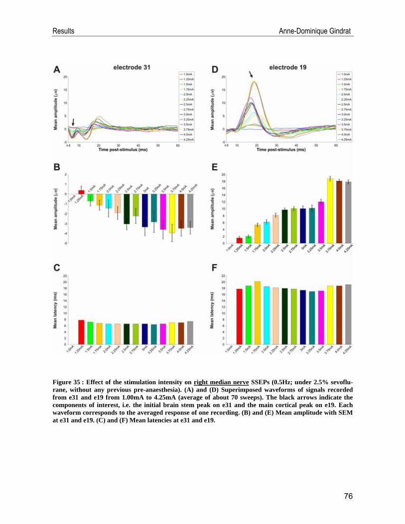
Results Anne-Dominique Gindrat
Figure 35 : Effect of the stimulation intensity on right median nerve SSEPs (0.5Hz; under 2.5% sevoflu-rane, without any previous pre-anaesthesia). (A) and (D) Superimposed waveforms of signals recorded from e31 and e19 from 1.00mA to 4.25mA (average of about 70 sweeps). The black arrows indicate the components of interest, i.e. the initial brain stem peak on e31 and the main cortical peak on e19. Each waveform corresponds to the averaged response of one recording. (B) and (E) Mean amplitude with SEM at e31 and e19. (C) and (F) Mean latencies at e31 and e19.
76
Results Anne-Dominique Gindrat
IV.1.5. Selection of the anaesthetic
In the first series of experiments, recordings were performed under K+D anaes-
thesia. As shown in Figure 36, recordings under this mix are not very stable during
the same session due to the difficulty to keep the depth of anaesthesia constant. The
recordings 1, 3 and 4 were obtained when the monkey was well anaesthetized. How-
ever, the morphology of the waveforms over the brain stem (on e32 in this case be-
cause recordings were not performed with the definitive cap yet) is not always con-
served across these recordings, as it could be expected from SSEPs acquired in the
same conditions without moving the stimulator between acquisitions (at 2.5% se-
voflurane, after pre-induction with D, remember Figure 25).The initial brain stem
component is for example not present in the first recording (Figure 36A, blue wave-
form). As far as the e19 is concerned (Figure 36D, E, F), the amplitude and the la-
tency of the cortical component are quite stable in these three recordings (amplitude
between 14.16 μV and 16.10 μV; latency between 16.4ms and 17.8ms) but the wave-
forms are not superimposed as well as in Figure 25. When the anaesthesia was only
light (recording 2), the amplitude of the cortical response was much larger than under
deeper anaesthesia. On the other hand, the amplitude of the initial brain stem com-
ponent was much lower. Therefore, these recording conditions were not optimal.
Figure 36 (next page): Evaluation of the stability under K+D anaesthesia of four scalp SSEPs from the same session, without changing the position of the stimulator between acquisitions, in response to right median nerve stimulation (1Hz frequency; 0.7mA intensity; average of 251-288 sweeps). (A) and (D) Waveforms of signals recorded from e32 and e19. In this session, at the beginning of the project, re-cordings were not performed with the definitive version of the cap and e32 was located in the midline, slightly above the brain stem. The black arrows indicate the components of interest, i.e. the initial brain stem peak on e32 and the main cortical peak on e19. Recording 1 (blue): 56min after K+D injection, the animal is well anaesthetized; recording 2 (red): 79min after K+D injection, the monkey begins to regain consciousness; recording 3 (green): 30min after reinjection of the mix, the animal is well anaesthetized; recording 4 (yellow): 50min after reinjection, the animal is well anaesthetized. (B) and (E) Mean ampli-tude with SEM at e32 and e19. (C) and (F) Mean latencies at e32 and e19.
77
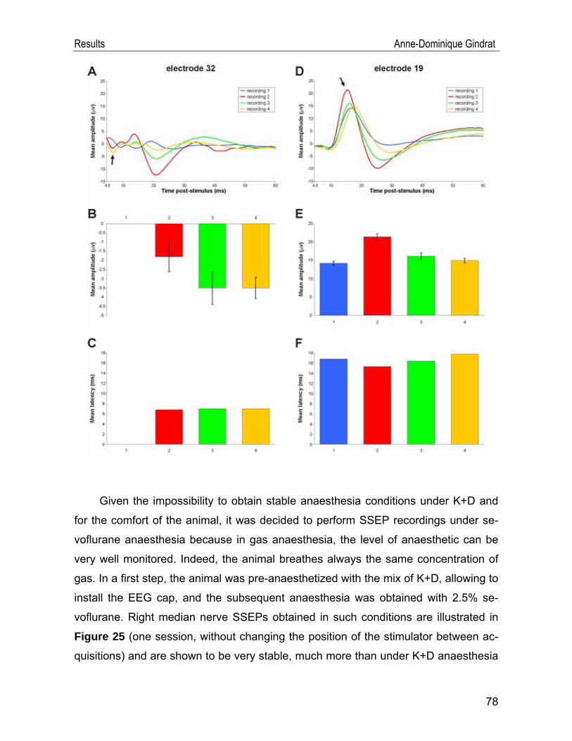
Results Anne-Dominique Gindrat
Given the impossibility to obtain stable anaesthesia conditions under K+D and
for the comfort of the animal, it was decided to perform SSEP recordings under se-
voflurane anaesthesia because in gas anaesthesia, the level of anaesthetic can be
very well monitored. Indeed, the animal breathes always the same concentration of
gas. In a first step, the animal was pre-anaesthetized with the mix of K+D, allowing to
install the EEG cap, and the subsequent anaesthesia was obtained with 2.5% se-
voflurane. Right median nerve SSEPs obtained in such conditions are illustrated in
Figure 25 (one session, without changing the position of the stimulator between ac-
quisitions) and are shown to be very stable, much more than under K+D anaesthesia
78

Results Anne-Dominique Gindrat
(Figure 36). Right median nerve SSEPs were also highly stable when recorded in a
same session at 2.5% sevoflurane after pre-induction of the anaesthesia with D only
(data not shown).
In the definitive protocol, to make the anaesthesia easier and for the comfort of
the animal, the sevoflurane anaesthesia alone was kept. Responses were shown to
be stable when recorded from the same session (Figures 27, 28) as well as from dif-
ferent sessions (Figures 29, 30) at 2.5% sevoflurane anaesthesia. Therefore, this
anaesthesia protocol was considered as the most reliable at that step.
However, a question persists : it is obvious that the sevoflurane level in the
blood does not change immediately after modifying the concentration. Therefore,
how long does it take to obtain a stable anaesthesia level once the gas concentration
has been modified ?
To answer this question, the gas concentration was lowered at 1.5% sevoflu-
rane after a quite long period at 2.5% sevoflurane in some recording sessions. The
transition from 2.5% down to 1.5% sevoflurane was evaluated in real time with right
tibial nerve SSEPs for half an hour (Figure 37). Changing the gas concentration from
2.5% to 1.5% sevoflurane has no influence on the amplitude of initial brain stem peak
on e31 (between -0.25μV and -0.85μV, Figure 37B), and no major influence on the
latency of this component (15ms at 2.5%, 13.8ms after 7-9min at 1.5%, 14.6ms after
13-15min, 15.8ms after 18-31ms, Figure 37C). As far as the cortical peak on e33 is
concerned, the amplitude increases as the gas concentration decreases, from
17.62μV to 23.66μV (Figure 37E) while the latency remains quite stable (between 28
and 29 ms, Figure 37F). We can therefore conclude that the gas concentration is still
not stable 30 minutes after the concentration transition for tibial nerve SSEPs. How-
ever, these results are based on a single recording session. Therefore, other acquisi-
tions are needed to confirm them.
79
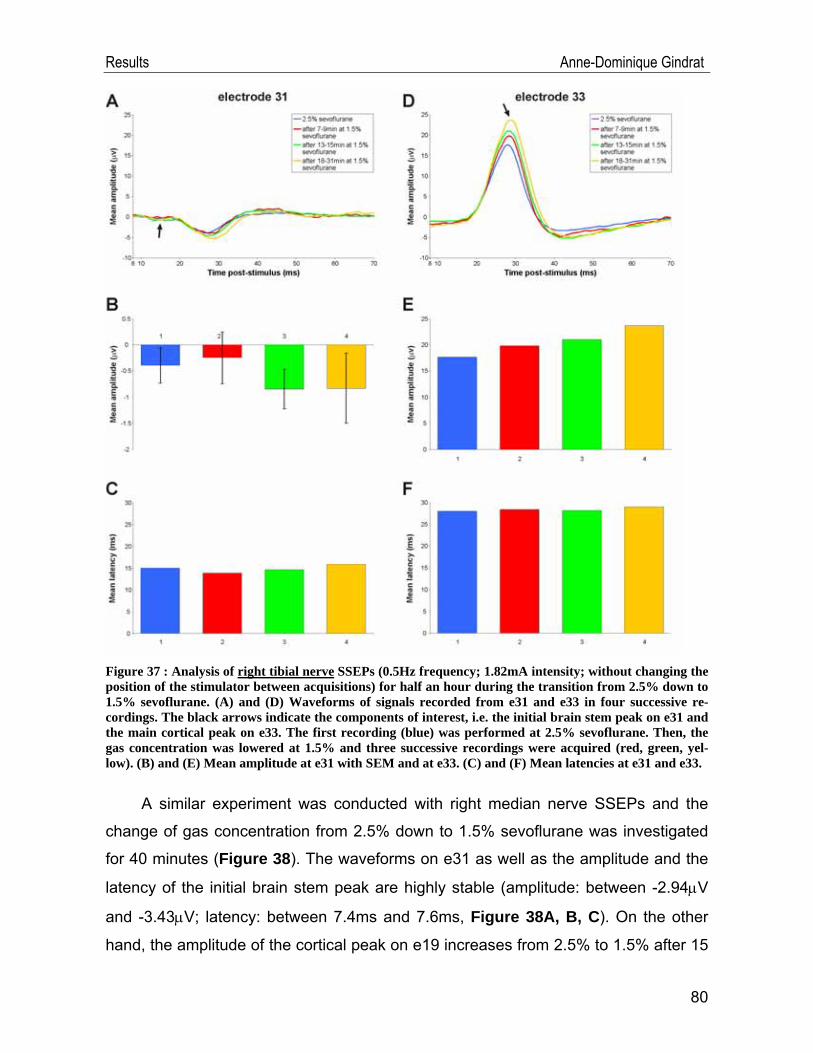
Results Anne-Dominique Gindrat
Figure 37 : Analysis of right tibial nerve SSEPs (0.5Hz frequency; 1.82mA intensity; without changing the position of the stimulator between acquisitions) for half an hour during the transition from 2.5% down to 1.5% sevoflurane. (A) and (D) Waveforms of signals recorded from e31 and e33 in four successive re-cordings. The black arrows indicate the components of interest, i.e. the initial brain stem peak on e31 and the main cortical peak on e33. The first recording (blue) was performed at 2.5% sevoflurane. Then, the gas concentration was lowered at 1.5% and three successive recordings were acquired (red, green, yel-low). (B) and (E) Mean amplitude at e31 with SEM and at e33. (C) and (F) Mean latencies at e31 and e33.
A similar experiment was conducted with right median nerve SSEPs and the
change of gas concentration from 2.5% down to 1.5% sevoflurane was investigated
for 40 minutes (Figure 38). The waveforms on e31 as well as the amplitude and the
latency of the initial brain stem peak are highly stable (amplitude: between -2.94μV
and -3.43μV; latency: between 7.4ms and 7.6ms, Figure 38A, B, C). On the other
hand, the amplitude of the cortical peak on e19 increases from 2.5% to 1.5% after 15
80
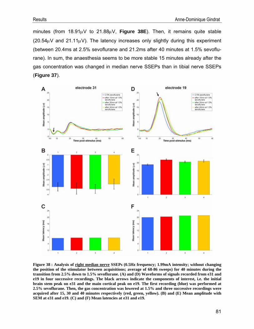
Results Anne-Dominique Gindrat
minutes (from 18.91μV to 21.88μV, Figure 38E). Then, it remains quite stable
(20.54μV and 21.11μV). The latency increases only slightly during this experiment
(between 20.4ms at 2.5% sevoflurane and 21.2ms after 40 minutes at 1.5% sevoflu-
rane). In sum, the anaesthesia seems to be more stable 15 minutes already after the
gas concentration was changed in median nerve SSEPs than in tibial nerve SSEPs
(Figure 37).
Figure 38 : Analysis of right median nerve SSEPs (0.5Hz frequency; 1.99mA intensity; without changing the position of the stimulator between acquisitions; average of 68-86 sweeps) for 40 minutes during the transition from 2.5% down to 1.5% sevoflurane. (A) and (D) Waveforms of signals recorded from e31 and e19 in four successive recordings. The black arrows indicate the components of interest, i.e. the initial brain stem peak on e31 and the main cortical peak on e19. The first recording (blue) was performed at 2.5% sevoflurane. Then, the gas concentration was lowered at 1.5% and three successive recordings were acquired after 15, 30 and 40 minutes respectively (red, green, yellow). (B) and (E) Mean amplitude with SEM at e31 and e19. (C) and (F) Mean latencies at e31 and e19.
81
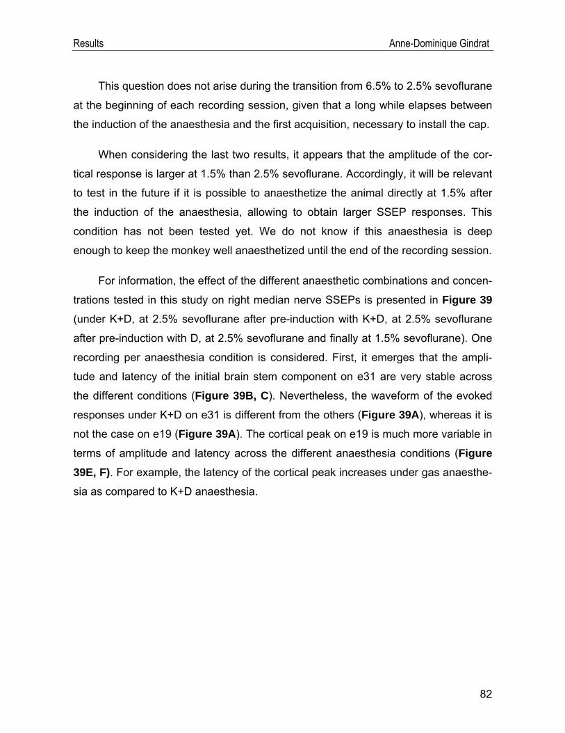
Results Anne-Dominique Gindrat
This question does not arise during the transition from 6.5% to 2.5% sevoflurane
at the beginning of each recording session, given that a long while elapses between
the induction of the anaesthesia and the first acquisition, necessary to install the cap.
When considering the last two results, it appears that the amplitude of the cor-
tical response is larger at 1.5% than 2.5% sevoflurane. Accordingly, it will be relevant
to test in the future if it is possible to anaesthetize the animal directly at 1.5% after
the induction of the anaesthesia, allowing to obtain larger SSEP responses. This
condition has not been tested yet. We do not know if this anaesthesia is deep
enough to keep the monkey well anaesthetized until the end of the recording session.
For information, the effect of the different anaesthetic combinations and concen-
trations tested in this study on right median nerve SSEPs is presented in Figure 39 (under K+D, at 2.5% sevoflurane after pre-induction with K+D, at 2.5% sevoflurane
after pre-induction with D, at 2.5% sevoflurane and finally at 1.5% sevoflurane). One
recording per anaesthesia condition is considered. First, it emerges that the ampli-
tude and latency of the initial brain stem component on e31 are very stable across
the different conditions (Figure 39B, C). Nevertheless, the waveform of the evoked
responses under K+D on e31 is different from the others (Figure 39A), whereas it is
not the case on e19 (Figure 39A). The cortical peak on e19 is much more variable in
terms of amplitude and latency across the different anaesthesia conditions (Figure 39E, F). For example, the latency of the cortical peak increases under gas anaesthe-
sia as compared to K+D anaesthesia.
82
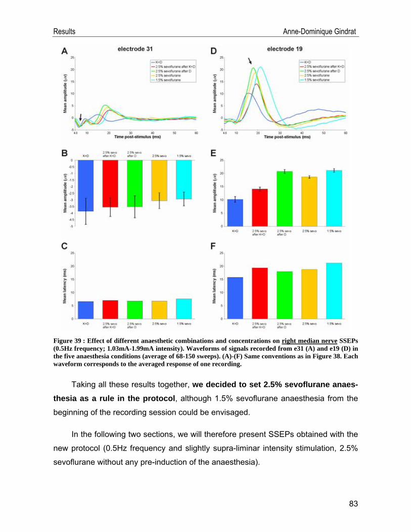
Results Anne-Dominique Gindrat
Figure 39 : Effect of different anaesthetic combinations and concentrations on right median nerve SSEPs (0.5Hz frequency; 1.03mA-1.99mA intensity). Waveforms of signals recorded from e31 (A) and e19 (D) in the five anaesthesia conditions (average of 68-150 sweeps). (A)-(F) Same conventions as in Figure 38. Each waveform corresponds to the averaged response of one recording.
Taking all these results together, we decided to set 2.5% sevoflurane anaes-thesia as a rule in the protocol, although 1.5% sevoflurane anaesthesia from the
beginning of the recording session could be envisaged.
In the following two sections, we will therefore present SSEPs obtained with the
new protocol (0.5Hz frequency and slightly supra-liminar intensity stimulation, 2.5%
sevoflurane without any pre-induction of the anaesthesia).
83
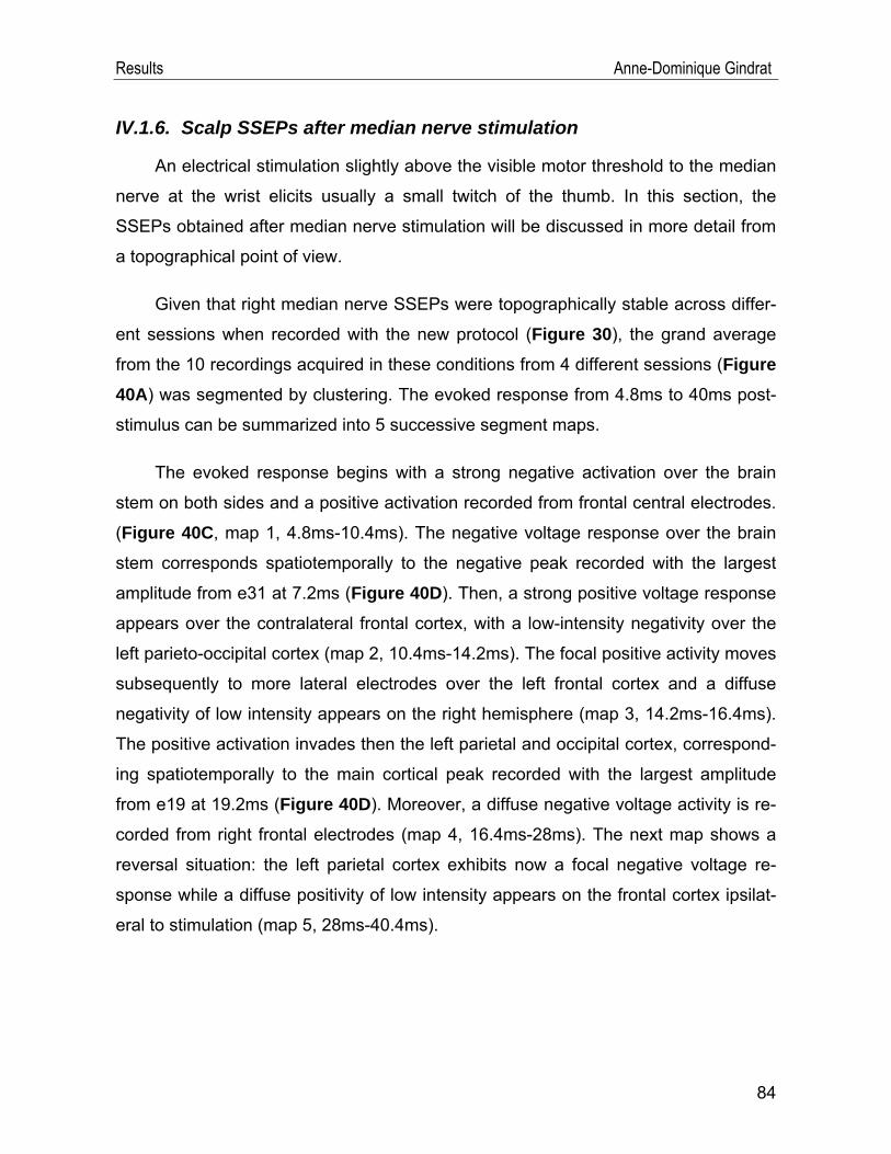
Results Anne-Dominique Gindrat
IV.1.6. Scalp SSEPs after median nerve stimulation
An electrical stimulation slightly above the visible motor threshold to the median
nerve at the wrist elicits usually a small twitch of the thumb. In this section, the
SSEPs obtained after median nerve stimulation will be discussed in more detail from
a topographical point of view.
Given that right median nerve SSEPs were topographically stable across differ-
ent sessions when recorded with the new protocol (Figure 30), the grand average
from the 10 recordings acquired in these conditions from 4 different sessions (Figure 40A) was segmented by clustering. The evoked response from 4.8ms to 40ms post-
stimulus can be summarized into 5 successive segment maps.
The evoked response begins with a strong negative activation over the brain
stem on both sides and a positive activation recorded from frontal central electrodes.
(Figure 40C, map 1, 4.8ms-10.4ms). The negative voltage response over the brain
stem corresponds spatiotemporally to the negative peak recorded with the largest
amplitude from e31 at 7.2ms (Figure 40D). Then, a strong positive voltage response
appears over the contralateral frontal cortex, with a low-intensity negativity over the
left parieto-occipital cortex (map 2, 10.4ms-14.2ms). The focal positive activity moves
subsequently to more lateral electrodes over the left frontal cortex and a diffuse
negativity of low intensity appears on the right hemisphere (map 3, 14.2ms-16.4ms).
The positive activation invades then the left parietal and occipital cortex, correspond-
ing spatiotemporally to the main cortical peak recorded with the largest amplitude
from e19 at 19.2ms (Figure 40D). Moreover, a diffuse negative voltage activity is re-
corded from right frontal electrodes (map 4, 16.4ms-28ms). The next map shows a
reversal situation: the left parietal cortex exhibits now a focal negative voltage re-
sponse while a diffuse positivity of low intensity appears on the frontal cortex ipsilat-
eral to stimulation (map 5, 28ms-40.4ms).
84
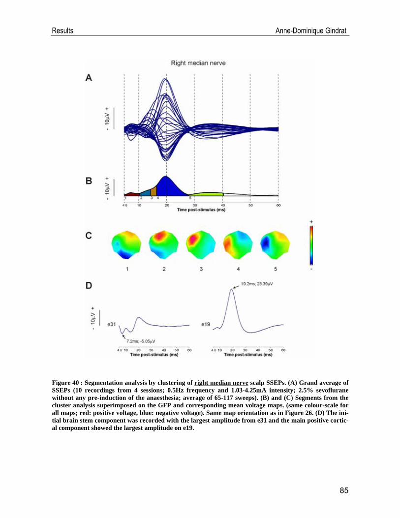
Results Anne-Dominique Gindrat
Figure 40 : Segmentation analysis by clustering of right median nerve scalp SSEPs. (A) Grand average of SSEPs (10 recordings from 4 sessions; 0.5Hz frequency and 1.03-4.25mA intensity; 2.5% sevoflurane without any pre-induction of the anaesthesia; average of 65-117 sweeps). (B) and (C) Segments from the cluster analysis superimposed on the GFP and corresponding mean voltage maps. (same colour-scale for all maps; red: positive voltage, blue: negative voltage). Same map orientation as in Figure 26. (D) The ini-tial brain stem component was recorded with the largest amplitude from e31 and the main positive cortic-al component showed the largest amplitude on e19.
85

Results Anne-Dominique Gindrat
The SSEP maps obtained in response to left median nerve stimulation are
based only on one recording (same protocol as for the right side) due to the few data
available (Figure 41). The spatiotemporal propagation of evoked activity is essen-
tially the mirror image to that obtained after stimulation on the right side, although the
segmentation on the left side is less complex (4 maps instead of 5 maps on the right
side) (Figure 41C). Maps 1 (4.8ms-13.4ms), 2 (13.4ms-18.2ms) and 3 (18.2ms-
31.2ms) of left median nerve SSEPs correspond quite well to maps 1, 2, and 4, re-
spectively, obtained on the right side (Figure 40), although the latency of appearance
of the maps is longer on the left side than on the right side (Figure 41B). Map 4
(31.2ms-26.6ms) of left side SSEPs, showing a negative activation over the right
fronto-parietal cortex and some positive activations over left fronto-parietal and oc-
cipital electrodes seems to correspond to map 5 of right side SSEPs.
In sum, median nerve SSEP maps correspond quite well from one side to the
other. The initial brain stem component is recorded in both cases with the largest
amplitude from contralateral brain stem electrodes, and the main positive component
is recorded with the largest amplitude from homologue contralateral parietal elec-
trodes (Figures 40D, Figure 41D). The slight differences observed in topography
and in component amplitude and latency are probably due to the fact that right me-
dian nerve SSEPs are based on a grand average of several recordings, while re-
sponses from the left side are obtained from a single recording, therefore more con-
taminated by noise (Figure 41A) than a grand average (Figure 40A). It is therefore
difficult to compare both situations and draw more conclusions.
86
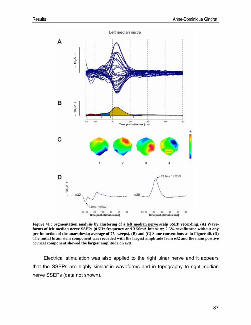
Results Anne-Dominique Gindrat
Figure 41 : Segmentation analysis by clustering of a left median nerve scalp SSEP recording. (A) Wave-forms of left median nerve SSEPs (0.5Hz frequency and 3.56mA intensity; 2.5% sevoflurane without any pre-induction of the anaesthesia; average of 75 sweeps). (B) and (C) Same conventions as in Figure 40. (D) The initial brain stem component was recorded with the largest amplitude from e32 and the main positive cortical component showed the largest amplitude on e20.
Electrical stimulation was also applied to the right ulnar nerve and it appears
that the SSEPs are highly similar in waveforms and in topography to right median
nerve SSEPs (data not shown).
87
Results Anne-Dominique Gindrat
IV.1.7. Scalp SSEPs after tibial nerve stimulation
A slightly supra-liminar electrical stimulation to the tibial nerve at the ankle elicits
usually a plantar flexion of the toes. The visible motor threshold is much lower than in
the case of median nerve stimulation.
Due to the few data available, a single right tibial nerve SSEP recording (ob-
tained with the new protocol mentioned above, Figure 42A) was segmented by clus-
tering. The evoked response from 20ms to 50ms post-stimulus can be summarized
into 2 successive segment maps (Figure 42B, C).
Map 1 (18.8ms-35.6ms) shows a strong focal activation over the central fronto-
parietal cortex. This corresponds spatiotemporally to the cortical peak recorded with
the largest amplitude from e33 at 28ms (Figure 42D). This positive activity goes with
some diffuse negative activities of very low intensity recorded from left and right pe-
ripheral electrodes and brain stem electrodes. Subsequently, the topographical or-
ganisation changes completely (map 2, 35.6ms-55.2ms): the central region of the
cap exhibits a strong negativity spreading also toward left parietal posterior cortex,
while some positive activations of low intensity appear on left parietal electrodes,
right parietal and occipital electrodes and electrodes over the brain stem.
Figure 42 (next page) : Segmentation analysis by clustering of a right tibial nerve scalp SSEP recording. (A) Waveforms of right tibial nerve SSEPs (0.5Hz frequency and 1.82mA intensity; 2.5% sevoflurane without any pre-induction of the anaesthesia; average of 80 sweeps). (B) and (C) Same conventions as in Figure 40. (D) The initial brain stem component was recorded with the largest amplitude from e31 and the main positive cortical component showed the largest amplitude on e33.
88
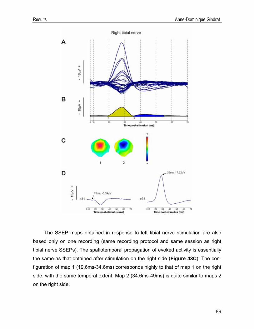
Results Anne-Dominique Gindrat
The SSEP maps obtained in response to left tibial nerve stimulation are also
based only on one recording (same recording protocol and same session as right
tibial nerve SSEPs). The spatiotemporal propagation of evoked activity is essentially
the same as that obtained after stimulation on the right side (Figure 43C). The con-
figuration of map 1 (19.6ms-34.6ms) corresponds highly to that of map 1 on the right
side, with the same temporal extent. Map 2 (34.6ms-49ms) is quite similar to maps 2
on the right side.
89
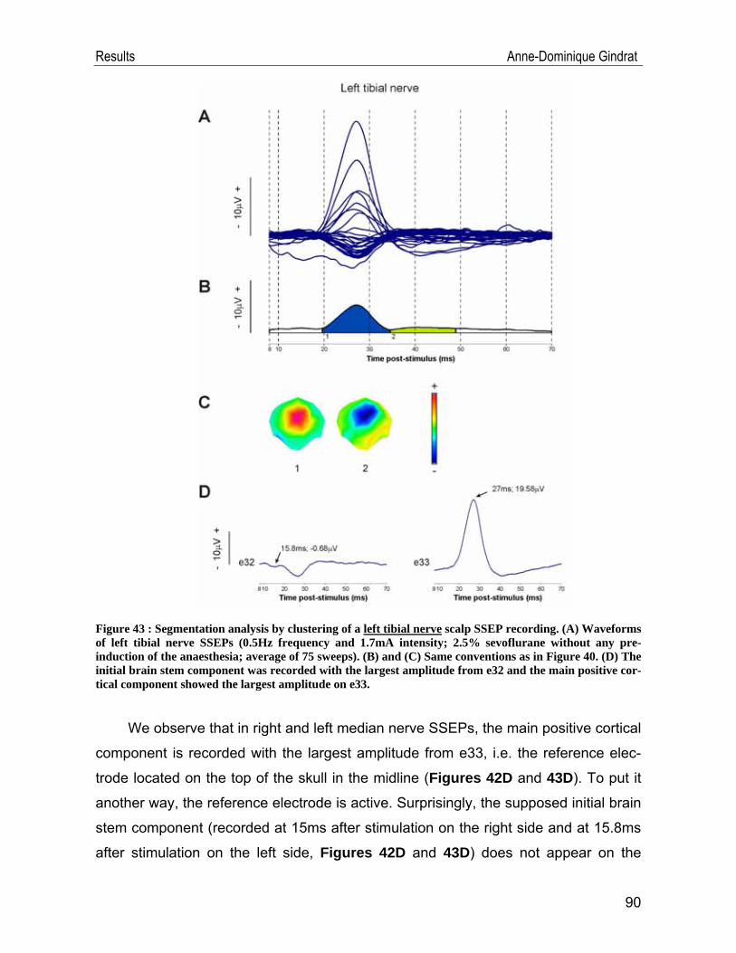
Results Anne-Dominique Gindrat
Figure 43 : Segmentation analysis by clustering of a left tibial nerve scalp SSEP recording. (A) Waveforms of left tibial nerve SSEPs (0.5Hz frequency and 1.7mA intensity; 2.5% sevoflurane without any pre-induction of the anaesthesia; average of 75 sweeps). (B) and (C) Same conventions as in Figure 40. (D) The initial brain stem component was recorded with the largest amplitude from e32 and the main positive cor-tical component showed the largest amplitude on e33.
We observe that in right and left median nerve SSEPs, the main positive cortical
component is recorded with the largest amplitude from e33, i.e. the reference elec-
trode located on the top of the skull in the midline (Figures 42D and 43D). To put it
another way, the reference electrode is active. Surprisingly, the supposed initial brain
stem component (recorded at 15ms after stimulation on the right side and at 15.8ms
after stimulation on the left side, Figures 42D and 43D) does not appear on the
90

Results Anne-Dominique Gindrat
SSEP maps of tibial nerve SSEPs, on the contrary to median nerve SSEPs (Figures 40D and 41D). It is probably because the reference electrode is very active at that
moment.
IV.2. Behavioural data
In parallel to the electrophysiological study, the behaviour of the monkey was
assessed daily with the modified Brinkman board task and the reach and grasp
drawer task.
IV.2.1. Modified Brinkman board task
The results of the modified Brinkman board task are presented here for a 146
days period. Some sessions corresponding to the training phase were however per-
formed already earlier but not recorded because coinciding with the beginning of
training the monkey to wear a cap on the head, with the intention of recording SSEPs
on the conscious monkey in the future. It was therefore quite difficult to acquire such
results because the animal was not familiar with the cap and the results were dis-
rupted by the monkey tearing it off.
The Figure 44A and B shows the score in 30s of each hand tested individual-ly, i.e. the number of pellets correctly retrieved throughout the first 30 seconds of the
task, and this score is considered separately in all slots, in vertical ones only and in
horizontal ones only. Given that the results are quite stable during this 146 days pe-
riod, the mean was computed over the totality of the sessions.
91
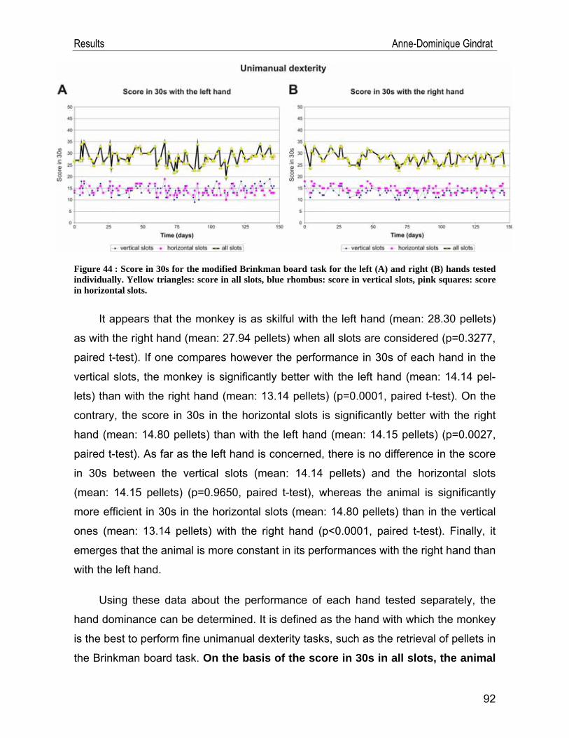
Results Anne-Dominique Gindrat
Figure 44 : Score in 30s for the modified Brinkman board task for the left (A) and right (B) hands tested individually. Yellow triangles: score in all slots, blue rhombus: score in vertical slots, pink squares: score in horizontal slots.
It appears that the monkey is as skilful with the left hand (mean: 28.30 pellets)
as with the right hand (mean: 27.94 pellets) when all slots are considered (p=0.3277,
paired t-test). If one compares however the performance in 30s of each hand in the
vertical slots, the monkey is significantly better with the left hand (mean: 14.14 pel-
lets) than with the right hand (mean: 13.14 pellets) (p=0.0001, paired t-test). On the
contrary, the score in 30s in the horizontal slots is significantly better with the right
hand (mean: 14.80 pellets) than with the left hand (mean: 14.15 pellets) (p=0.0027,
paired t-test). As far as the left hand is concerned, there is no difference in the score
in 30s between the vertical slots (mean: 14.14 pellets) and the horizontal slots
(mean: 14.15 pellets) (p=0.9650, paired t-test), whereas the animal is significantly
more efficient in 30s in the horizontal slots (mean: 14.80 pellets) than in the vertical
ones (mean: 13.14 pellets) with the right hand (p<0.0001, paired t-test). Finally, it
emerges that the animal is more constant in its performances with the right hand than
with the left hand.
Using these data about the performance of each hand tested separately, the
hand dominance can be determined. It is defined as the hand with which the monkey
is the best to perform fine unimanual dexterity tasks, such as the retrieval of pellets in
the Brinkman board task. On the basis of the score in 30s in all slots, the animal
92
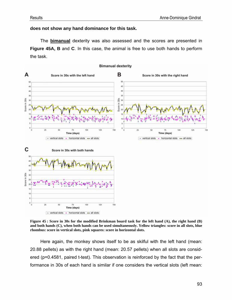
Results Anne-Dominique Gindrat
does not show any hand dominance for this task.
The bimanual dexterity was also assessed and the scores are presented in
Figure 45A, B and C. In this case, the animal is free to use both hands to perform
the task.
Figure 45 : Score in 30s for the modified Brinkman board task for the left hand (A), the right hand (B) and both hands (C), when both hands can be used simultaneously. Yellow triangles: score in all slots, blue rhombus: score in vertical slots, pink squares: score in horizontal slots.
Here again, the monkey shows itself to be as skilful with the left hand (mean:
20.88 pellets) as with the right hand (mean: 20.57 pellets) when all slots are consid-
ered (p=0.4581, paired t-test). This observation is reinforced by the fact that the per-
formance in 30s of each hand is similar if one considers the vertical slots (left mean:
93

Results Anne-Dominique Gindrat
94
10.08 pellets; right mean: 10.27 pellets; p=0.6323, paired t-test) or the horizontal
slots (left mean: 10.80 pellets; right mean: 10.30 pellets; p=0.0928, paired t-test). As
far as the left hand is concerned, the animal retrieves significantly more pellets in 30s
from the horizontal slots (mean: 10.80 pellets) than in the vertical ones (mean: 10.08
pellets) (p=0.0216). On the other hand, there is no significant difference in the score
in 30s between the vertical slots (mean: 10.27 pellets) and the horizontal slots
(mean: 10.30 pellets) with the right hand (p=0.9347, paired t-test). Finally, in the bi-
manual tests, the monkey seems to have more constant performances with the left
hand than the right hand.
These data allow to establish the hand preference of the monkey, defined as
the hand preferentially used to perform a task when both are available: if one con-siders all slots together as well as the vertical slots only or the horizontal slots only, the animal does not show any hand preference for this task. This observa-
tion goes in the same direction as the fact that the monkey does not have any hand
dominance.
As suggested by Pauline Chatagny (2009), the hand dominance and the hand
preference can also be assessed by calculating the contact time of the fingers in the
slots, besides the score in 30s. However, as the behavioural tests are not the major
topic of this project, these results will not be presented here.
IV.2.2. Reach and grasp drawer task
The force of the animal was evaluated individually for each hand with the reach
and grasp drawer task, performed during a 133 days period (from day 14 to day 146
of the Brinkman task). Five resistance levels were tested: 0, 3, 5, 7 and 10, corre-
sponding in Newtons to 0N, 1.35N, 2.8N, 5N and 9N respectively (static load force
measures). At resistance 10, the task was very difficult, even impossible the first
days, especially for the left hand. It should be mentioned that the drawer setup was
serviced from day 108 to day 110, and after that, some measures, especially the pull-
ing time, were modified. The reason is unknown.
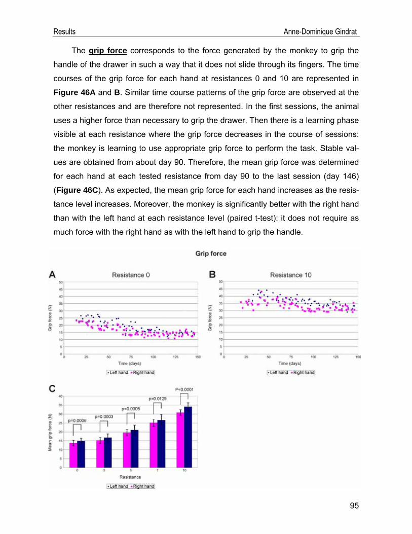
Results Anne-Dominique Gindrat
The grip force corresponds to the force generated by the monkey to grip the
handle of the drawer in such a way that it does not slide through its fingers. The time
courses of the grip force for each hand at resistances 0 and 10 are represented in
Figure 46A and B. Similar time course patterns of the grip force are observed at the
other resistances and are therefore not represented. In the first sessions, the animal
uses a higher force than necessary to grip the drawer. Then there is a learning phase
visible at each resistance where the grip force decreases in the course of sessions:
the monkey is learning to use appropriate grip force to perform the task. Stable val-
ues are obtained from about day 90. Therefore, the mean grip force was determined
for each hand at each tested resistance from day 90 to the last session (day 146)
(Figure 46C). As expected, the mean grip force for each hand increases as the resis-
tance level increases. Moreover, the monkey is significantly better with the right hand
than with the left hand at each resistance level (paired t-test): it does not require as
much force with the right hand as with the left hand to grip the handle.
95

Results Anne-Dominique Gindrat
Figure 46 (previous page) : Grip force generated in the reach and grasp drawer task. Time course of the grip force generated at drawer resistances 0 (A) and 10 (B). Blue rhombus: left hand, pink squares: right hand. The time scale corresponds to the one in Brinkman tests. The data were acquired from day 14. At resistance 10, no data are available in the first sessions because the animal was unable to perform the task. (C) Mean grip forces (from day 90 to day 146) with standard deviations for each hand at each resistance level tested. A bilateral paired t-test (confidence interval: 95%) was performed between both hands at each resistance and p values are indicated. Blue: left hand, pink: right hand.
The load force represents the force the animal needs to pull the drawer and
consequently must be higher than the resistance of the drawer. The reader should
nevertheless pay attention to the fact that the drawer resistances given in N corre-
spond to static load force measures and not dynamic measures and can therefore
not be directly compared with the load forces. The Figure 47A and B shows the time
courses of the load force for each hand at resistances 3 and 5. Similar patterns are
obtained at the others resistances. Contrary to the grip force, there is few learning
effect, visible only at resistances 0 and 3. At both these resistances, the animal gen-
erates a similar basic load force larger than necessary in the first sessions, meaning
that it does not adapt the load force for null or weak resistances in the first sessions.
Then, in the following days, it leans to adapt the required force to the task. A similar
remark applies to the grip force at resistances 0 and 3 for the right hand. The load
force is stable in time at resistances 5, 7 and 10. In the last sessions however, the
load force shows an increase at each resistance, especially for the right hand. There-
fore, the mean load force was determined from day 90 to day 125 only (Figure 47C).
As expected here again, the mean load force for each hand increases as the resis-
tance level increases. Furthermore, the monkey generates significantly lower load
forces with the right hand than with the left hand at resistances 0, 3, and 10 whereas
the performances between both hands are similar at resistances 5 and 7 (paired t-
test). By comparison, the monkey uses a lower grip force with the right hand than
with the left one at each resistance, as shown above (Figure 46C).
96
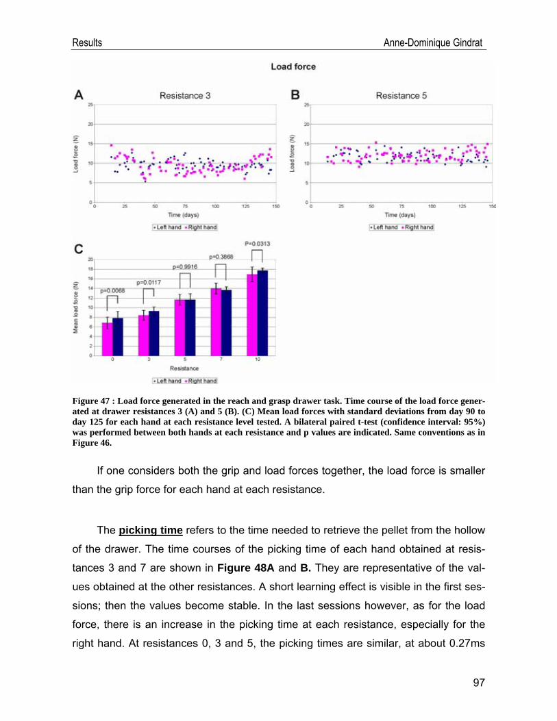
Results Anne-Dominique Gindrat
Figure 47 : Load force generated in the reach and grasp drawer task. Time course of the load force gener-ated at drawer resistances 3 (A) and 5 (B). (C) Mean load forces with standard deviations from day 90 to day 125 for each hand at each resistance level tested. A bilateral paired t-test (confidence interval: 95%) was performed between both hands at each resistance and p values are indicated. Same conventions as in Figure 46.
If one considers both the grip and load forces together, the load force is smaller
than the grip force for each hand at each resistance.
The picking time refers to the time needed to retrieve the pellet from the hollow
of the drawer. The time courses of the picking time of each hand obtained at resis-
tances 3 and 7 are shown in Figure 48A and B. They are representative of the val-
ues obtained at the other resistances. A short learning effect is visible in the first ses-
sions; then the values become stable. In the last sessions however, as for the load
force, there is an increase in the picking time at each resistance, especially for the
right hand. At resistances 0, 3 and 5, the picking times are similar, at about 0.27ms
97
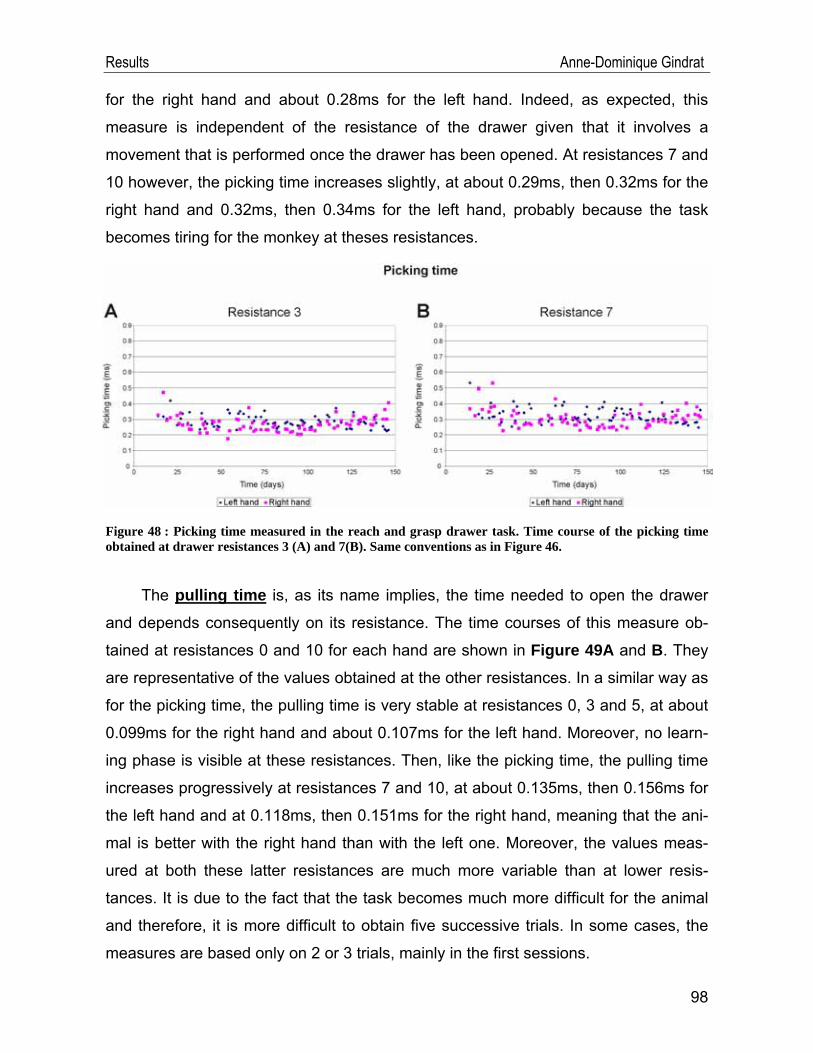
Results Anne-Dominique Gindrat
for the right hand and about 0.28ms for the left hand. Indeed, as expected, this
measure is independent of the resistance of the drawer given that it involves a
movement that is performed once the drawer has been opened. At resistances 7 and
10 however, the picking time increases slightly, at about 0.29ms, then 0.32ms for the
right hand and 0.32ms, then 0.34ms for the left hand, probably because the task
becomes tiring for the monkey at theses resistances.
Figure 48 : Picking time measured in the reach and grasp drawer task. Time course of the picking time obtained at drawer resistances 3 (A) and 7(B). Same conventions as in Figure 46.
The pulling time is, as its name implies, the time needed to open the drawer
and depends consequently on its resistance. The time courses of this measure ob-
tained at resistances 0 and 10 for each hand are shown in Figure 49A and B. They
are representative of the values obtained at the other resistances. In a similar way as
for the picking time, the pulling time is very stable at resistances 0, 3 and 5, at about
0.099ms for the right hand and about 0.107ms for the left hand. Moreover, no learn-
ing phase is visible at these resistances. Then, like the picking time, the pulling time
increases progressively at resistances 7 and 10, at about 0.135ms, then 0.156ms for
the left hand and at 0.118ms, then 0.151ms for the right hand, meaning that the ani-
mal is better with the right hand than with the left one. Moreover, the values meas-
ured at both these latter resistances are much more variable than at lower resis-
tances. It is due to the fact that the task becomes much more difficult for the animal
and therefore, it is more difficult to obtain five successive trials. In some cases, the
measures are based only on 2 or 3 trials, mainly in the first sessions.
98
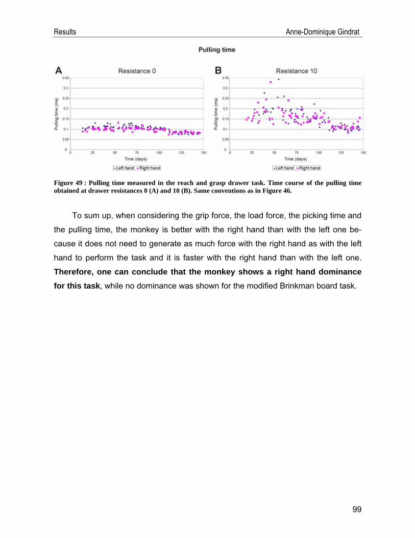
Results Anne-Dominique Gindrat
Figure 49 : Pulling time measured in the reach and grasp drawer task. Time course of the pulling time obtained at drawer resistances 0 (A) and 10 (B). Same conventions as in Figure 46.
To sum up, when considering the grip force, the load force, the picking time and
the pulling time, the monkey is better with the right hand than with the left one be-
cause it does not need to generate as much force with the right hand as with the left
hand to perform the task and it is faster with the right hand than with the left one.
Therefore, one can conclude that the monkey shows a right hand dominance for this task, while no dominance was shown for the modified Brinkman board task.
99
Discussion Anne-Dominique Gindrat
V. Discussion The general context of this project was the development of a minimally invasive
method to investigate repeatedly the brain activity in macaque monkey in relation to a
central nervous system lesion. Multichannel scalp SSEPs were used and the aim
was to adjust all the recording parameters allowing to suggest an improved recording
protocol as compared to the previous SSEP technique used in the laboratory, re-
stricted to corticography above a limited brain area, M1 and S1 on one side (Kaeser
et al., 2006, 2007). We demonstrated that scalp multichannel SSEPs can be re-
corded in anesthetized monkey and will be relevant in the future to long-term as-
sessment of cortical activity after a lesion.
V.1. SSEP data
V.1.1. Stability of the SSEPs
To evaluate whether multichannel scalp SSEPs could be used for repeated as-
sessment of the brain activity, the stability of the responses obtained under sevoflu-
rane anaesthesia was investigated within and across recording sessions. We showed
that the SSEPs were highly reproducible in terms of amplitude, latency and topogra-
phy (Figures 25 and 26) when recorded from the same session with the stimulator
staying at the same place (under sevoflurane anaesthesia and not under K+D anaes-
thesia), as expected, given that all the recordings conditions were the same.
When the stimulator was moved between each acquisition in the same session
(Figures 27 and 28), the responses were slightly more variable when the waveforms
were considered but highly stable from a topographical point of view. In this case, the
small differences in amplitude and latencies visible on e19 are probably due to the
fact that the stimulator was not repositioned exactly at the same place for each ac-
quisition and consequently the stimulation intensity should be readjusted every time
to obtain a small visible twitch of the fingers. Indeed, we saw that the possibility to
observe a visible motor response is very sensitive to the location of the stimulator.
Moving the stimulator only slightly could completely abolish or on the contrary en-
hance the motor response if the stimulation intensity was not readjusted. Neverthe-
100
Discussion Anne-Dominique Gindrat
less, given that the topography of the maps was very well conserved, it seems that
the repositioning of the stimulator between acquisitions does not constitute an impor-
tant problem.
In recordings obtained from different sessions (Figures 29 and 30), the ampli-
tude and latency changes observed are due to the fact that here again, the stimulator
was not exactly at the same location and therefore the stimulation intensity varied.
Moreover, we are not sure that the cap was exactly positioned at the same place at
the scalp for each session. The variable number of sweeps averaged seems not to
play a role here (remember Figure 34). The cortical component on the first recording
was much smaller than in the next sessions, probably because it was the first ses-
sion in these conditions and the method was not completely well designed yet. The
most obvious difference in the responses across all sessions is the shift in latency of
the waveforms and of the GFP. It seems that there are two groups of recordings. The
first three sessions were performed under hot weather condition, increasing the con-
duction speed and therefore decreasing the latency of the components. On the con-
trary, in the two last sessions, the room temperature was colder, increasing the con-
duction time and the latency of the SSEP components. It is therefore possible that
the room temperature, and therefore the body temperature of the animal, had an in-
fluence on the latency of the components, as mentioned for example by Banoub et
al. (2003) and Mauguière (2005). Other factors of the internal state of the animal
could play a role (slight differences in anaesthesia level between sessions). The shift
in latency is smaller for the initial brain stem peak than for the cortical peak. This is
expected given that the cortical peak appears later than the initial brain stem peak
and therefore the delay accumulates as the latency increases.
But here again, although there were some changes in the waveforms, the to-
pography was well conserved across the sessions, what proves that our technique is
valid and can be used in long term assessment of the cortical activity in monkey.
Moreover, it shows the importance of the topographical analysis associated with the
conventional waveform analysis: both are complementary, providing different infor-
mation. The waveform analysis is not sufficient to determine if the results are repro-
101
Discussion Anne-Dominique Gindrat
ducible or not, but topographical analysis is required. This discrepancy between the
results of the waveform analysis and those of the topographical analysis (and the
GFP waveform) across the sessions is due to the fact that the same difference in
amplitude and latency is probably present in each component of each electrode in a
recording, as compared to another recording. Therefore, the relative amplitudes,
consequently the GFP amplitudes and the map topographies are the same in both
cases, despite a delay in latency.
SSEP experiments were performed in other species, as for example epicranial
SSEP recordings in response to stimulation of the whiskers in mice (Mégevand et al.,
2008; Troncoso et al., 2000). In this case, the evoked responses were highly stereo-
typed from one session to the other (Mégevand et al., 2008), more than in our study
because in these rodent experiments, epicranial recordings were performed with an
electrode grid positioned always exactly in the same way and the stimulation condi-
tions were exactly the same.
These experiments were essential to show that the SSEPs are stable even
across the recording sessions and consequently it will be possible to distinguish the
actual effects of a lesion and a treatment on these responses.
V.1.2. Factors influencing the SSEPs
Stimulation frequency: it is reported in human that the SSEP peak amplitude
declines as the stimulation frequency increases while the latency is not affected
(Araki et al., 1999). In our study, we observed indeed that the amplitude of the corti-
cal response decreased as the stimulation repetition rate increased (Figure 32).
However, we reported in parallel a small increase in response latency. Exactly the
same phenomenon was described in rodents after whisker stimulation (Stienen et al.,
2003). The effect of the stimulation frequency was also visible on individual sweeps
(Figure 33), but contrary to rodent EPs after mechanical whiskers stimulation where
the amplitude of the responses becomes already stable after 3 or 4 stimulations
(Quairiaux et al., 2007), the amplitude seems to fall in the first 30 sweeps at 1Hz and
at 2Hz in our study.
102
Discussion Anne-Dominique Gindrat
Stimulation intensity: we observed that the response amplitude was the largest
at slightly supra-liminar intensity to evoke a movement of fingers or toes (Figure 35).
This result is in accordance with Mauguière and Fischer (1990) who reported the
same phenomenon in human. We also observed that when the stimulation intensity
increased too much above the threshold, the amplitude of the SSEPs decreased, a
phenomenon explained by the occlusion of Ia impulse traffic (Aminoff and Eisen,
1998). It is important to obtain responses with amplitude as large as possible be-
cause, as explained by Banoub et al. (2003), the SSEP reproducibility depends di-
rectly on the component amplitude and inversely on the amplitude variability. To put it
another way, the smaller the amplitude of the components is, the more variable it is,
influenced by baseline variations, electrical noise, and other factors. Freye (2005)
mentioned that changes in stimulation intensity have no impact on the component
latency. Nevertheless, we observed changes in latency as the stimulation intensity
changed, mainly for the cortical component. Interestingly, the smallest latency of the
initial brain stem component and cortical peak was observed at the visible motor
threshold.
Anaesthesia: recordings were performed with different anaesthesia conditions
and the initial brain stem component was only slightly affected in amplitude and la-
tency, whereas the main cortical component was susceptible to the tested anaesthe-
sia (Figures 36-39). This result is in accordance with studies in human (Berger and
Blum, 2007; Vaughan et al., 2001). The effect of K+D on the SSEPs is difficult to
analyse given that few data are available and they are variable. Nevertheless, as
mentioned by Banoub et al. (2003), it seems that the K anaesthesia is less depres-
sive than the gas anaesthesia because the latency of the main cortical component
was shorter under K+D than under sevoflurane (Figure 39E). However, the ampli-
tude was smaller under K+D than under sevoflurane, maybe due to the interaction of
K with D.
Different concentrations of sevoflurane were tested (2.5% and 1.5%) and we
observed that the cortical response had a larger amplitude under lighter than deeper
anaesthesia. This dose-dependant effect of sevoflurane on cortical SSEP is particu-
103
Discussion Anne-Dominique Gindrat
104
larly well visible on Figure 37D, E. These results are consistent with human data
(Banoub et al., 2003). However, we observed an increase in cortical latency as the
gas concentration decreased (Figures 38E, 39E), what is surprising. A cluster analy-
sis of rodent whisker EPs showed even that responses were less complex under
deep gas anaesthesia than under light anaesthesia (Mégevand et al., 2008). This
aspect was however not studied here due to the few available recordings obtained at
1.5% sevoflurane. After changing the gas concentration from 2.5% to 1.5% sevoflu-
rane, we observed that median nerve SSEPs were already quite stable 15 minutes
after the concentration modulation (Figure 38), whereas the cortical component of
tibial nerve SSEPs increased in amplitude still half an hour after concentration
change (Figure 37). In human however, it takes only 5-8 minutes to obtain a stable
cortical response after concentration modulation (Banoub et al., 2003). Our results
are however based each on a single experiment. Therefore, they should be repeated.
It emerges that for each tested parameter, the initial brain stem component was
much less influenced than the cortical component.
In sum, our scalp SSEP technique is a sensitive enough approach to resolve dif-
ferences in waveforms when different conditions are tested.
V.1.3. Interpretation of scalp SSEP maps
Before going into details of the maps, it should be mentioned that not every vol-
tage maximum or minimum visible on the maps is produced by an individual genera-
tor, especially if the activity is spatially diffuse rather than focal (Mégevand et al.,
2008). In fact, it is possible that two activations visible on the same maps, a positive
one and a negative one, correspond each to one pole of the same dipole produced
by a single generator. Moreover, the activation recorded at the scalp does not always
correspond to an activity of the neurons located directly under the recording elec-
trodes. The electrodes can also record far-field potentials. Finally, similar surface to-
pographies are not necessarily due to the same generators but may be produced by
different neuronal sources (Michel et al., 2004).
Discussion Anne-Dominique Gindrat
Our data suggest that an electrical stimulation to the median nerve activates
mainly the contralateral hemisphere, as expected. The maps produced in response
to right median nerve stimulation will be discussed (Figure 40). The maps obtained
from left side stimulation (Figure 41) are interpreted in the same way given that there
are nearly mirror images of those of the right side in relation to the antero-posterior
axis.
For map 1 showing a strong negative activation over the most posterior elec-
trodes on both sides at about 7ms, we most probably recorded the early processing
of the afferent volley in the dorsal column nuclei in the brain stem, before arriving in
cortical structures, as shown in human (Lascano et al., 2009) (see Figure 50 below).
On the other hand, it is difficult to explain the positive activation recorded from fron-
talmost central electrodes.
Then, maps 2 and 3 are characterized by a focal positive voltage response over
the contralateral fronto-parietal cortex whose amplitude is much stronger than the
negative activation also visible on these maps. This configuration could be due to a
dipole located between both activities. Does the positive activation correspond to a
response of M1 or of a frontal region? It is possible. In this case, it would be consis-
tent with high-resolution SSEP data obtained in human in the laboratory of Prof C.M.
Michel, which show that after an electrical stimulation to the median nerve, but not
after a pneumatic stimulation, the motor cortex and frontal regions are activated be-
fore or at the same time as sensory areas (data not published). It could be due to di-
rect thalamo-cortical inputs to frontal regions, such as proprioceptive fibres which are
known to be activated after an electrical stimulation (Allison et al., 1991a; Cohen et
al., 1981; Cruccu et al., 2008; Cusick et al., 1979; Freye, 2005; Legatt and Soliman,
2006) and that convey sensory information to the motor cortex. It could also reflect
the activation of another cortical area in the contralateral hemisphere whose exact
location remains to be determined.
Map 4 shows a positive activation invading the left parietal and occipital cortices
(main cortical peak at 19ms) and a diffuse negative voltage activity recorded from
105
Discussion Anne-Dominique Gindrat
right frontal electrodes. This is most probably due to a dipole with the positive pole in
the contralateral somatosensory cortex and the negative counterpart in the ipsilateral
hemisphere, as shown in human (see Figure 50 below). In this case, the activation in
S1 could be due to cortico-cortical fibres from M1 to S1 or to a later thalamo-cortical
activation.
The reversal situation visible in map 5 as compared to map 4 is difficult to inter-
pret: it is possible that this change in intracerebral activity at the level of the genera-
tors is only due to the main source which moved from one cortical layer to another in
the same region. It is also possible that the activation visible in map 4 is followed by a
deactivation. Based on the fact that it seems that map 5 shows a polarity inversion as
compared to map 4, one could also propose that it is due to an inversion in the di-
pole, as seen sometimes in spontaneous oscillatory activity. All these hypotheses are
valuable and there is no evidence until now to support any of them.
As expected, responses evoked by electrical stimulation to the tibial nerve are
completely different from those of the median nerve. The latency of the initial brain
stem component and of the main cortical response is logically much longer in tibial
nerve SSEPs than in median nerve SSEPs, given that the sensory pathway is much
longer from the ankle to the brain than from the wrist to the brain. If one considers
responses from the right side, it seems that there is a latency difference of about 8-
9ms: the initial brain stem component appears at about 7ms after simulation of the
upper limb and at about 15ms after stimulation of the lower limb. In the same way,
the main cortical component is visible after about 19ms in median nerve SSEPs, as
compared to about 28ms in tibial nerve SSEPs. However, the results of the tibial
nerve stimulation must be considered with caution given that they are obtained from
a single recording. For the same reason, the comparison between left upper and
lower limb response latency is also subjected to caution. Here again, the results of
right tibial nerve stimulation (Figure 42) only will be discussed given that responses
from the left side (Figure 43) are very similar.
Map 1 of right tibial nerve SSEPs (Figure 42) shows a strong centro-parietal
positive field at the midline, corresponding probably to a tangential dipole in the leg
106
Discussion Anne-Dominique Gindrat
107
area of the sensorimotor cortex, as reported in human (Berger and Blum, 2007;
Cruccu et al., 2008; Erwin et al., 1987). Both hemispheres seem to be activated: it is
due to the fact that the leg area is located in the medial aspect of the sensorimotor
cortex (Figure 10), along the longitudinal cerebral fissure, and therefore, electrodes
over this region on both sides record the same positive response.
Map 2 may be interpreted in the same way as map 5 in median nerve SSEPs
because here again, a reversal configuration is observed as compared to the previ-
ous map.
As mentioned before, our reference electrode e33 is active because it records
the main cortical peak with the largest amplitude after stimulation to the tibial nerve,
meaning that the activity is probably located just underneath. To put it another way,
this electrode may be located just above the leg area in the sensorimotor cortex. For
some authors, it constitutes a major problem (see for example Desmedt, 1987) and
they recommend to use a reference located over a non-active zone. But in fact, there
is no problem in our case given that all recordings were performed in this condition
and the average reference was used instead of the physical reference (Michel et al.,
2004; Murray et al., 2008) (see Introduction p.25).
All the interpretations of the topographical data presented here based on hu-man SSEP data interpretations. The only way to verify all these hypotheses with
certainty would have been to perform intracortical recordings to analyse the current
source density (Erwin et al., 1987; Mégevand et al., 2008) but it was not the goal
here. A non-invasive way would be to solve an inverse solution allowing to localize
the neural generators and show their orientation (Michel et al., 1999, 2001, 2004).
In the future, it will be required to acquire more recordings at each site to com-
pute grand averages and then segmentation analyses. We observed indeed that
segmentations based on a single recording were not optimal because the signal to
noise ratio was higher than with a grand average.
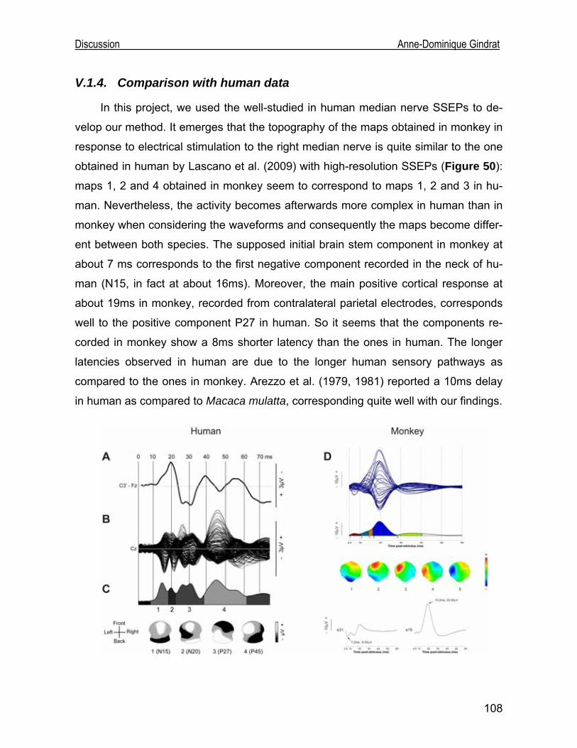
Discussion Anne-Dominique Gindrat
V.1.4. Comparison with human data
In this project, we used the well-studied in human median nerve SSEPs to de-
velop our method. It emerges that the topography of the maps obtained in monkey in
response to electrical stimulation to the right median nerve is quite similar to the one
obtained in human by Lascano et al. (2009) with high-resolution SSEPs (Figure 50):
maps 1, 2 and 4 obtained in monkey seem to correspond to maps 1, 2 and 3 in hu-
man. Nevertheless, the activity becomes afterwards more complex in human than in
monkey when considering the waveforms and consequently the maps become differ-
ent between both species. The supposed initial brain stem component in monkey at
about 7 ms corresponds to the first negative component recorded in the neck of hu-
man (N15, in fact at about 16ms). Moreover, the main positive cortical response at
about 19ms in monkey, recorded from contralateral parietal electrodes, corresponds
well to the positive component P27 in human. So it seems that the components re-
corded in monkey show a 8ms shorter latency than the ones in human. The longer
latencies observed in human are due to the longer human sensory pathways as
compared to the ones in monkey. Arezzo et al. (1979, 1981) reported a 10ms delay
in human as compared to Macaca mulatta, corresponding quite well with our findings.
108
Discussion Anne-Dominique Gindrat
Figure 50 (previous page) : Comparison of right median nerve SSEPs obtained with an electrical stimula-tion in human (A-C) and in monkey (D). The human data are averaged from 29 healthy people and rec-orded from 204 electrodes referenced to the average reference (B). (A) Waveform recorded from a contra-lateral centroparietal electrode referenced here to the frontal electrode Fz (C3’-Fz) and corresponding probably to e19 in monkey. (C) The temporal extent of the four segment maps resulting from a cluster analysis (k-mean segmentation) of the grand average (B) is shown as grey-coded segments on the GFP trace. The voltage topographies are shown below. Map scale: white, positive voltage; black, negative vol-tage. (D) See Figure 40 p.85 (A-C from Lascano et al., 2009).
In their human study, Lascano et al. (2009) demonstrated that the topography of
left median nerve SSEP maps is nearly the mirror image of the one obtained for the
right side, in relation to the antero-posterior axis. The same observation was made in
our monkey study, although there were some latency differences between both
sides. Nevertheless, we can not make conclusion about this latency difference given
that the left median nerve cluster analysis is based only on a single recording.
As far as tibial nerve SSEP maps are concerned, our data will be compared to
the ones obtained in human by van de Wassenberg et al. (2008). As shown in Figure 51, the configuration of both maps obtained in monkey in response to electrical
stimulation to the right tibial nerve is quite similar to the one of the first two maps ob-
tained in human with high-resolution SSEPs. The main positive cortical response in
monkey, recorded from midline centro-parietal electrodes, corresponds well to the
positive component P39 recorded in human, appearing in fact at about 44ms, al-
though the positive activation in human extents toward more occipital sites. Then the
central negativity, recorded at about 42ms in the monkey, corresponds to the com-
ponent N50 in human, appearing at about 54ms. Here again, the later activity seems
more complex in human than in monkey. In this case, it is however difficult to com-
pare precisely the latencies between both species given that the monkey maps are
based on a single recording.
109
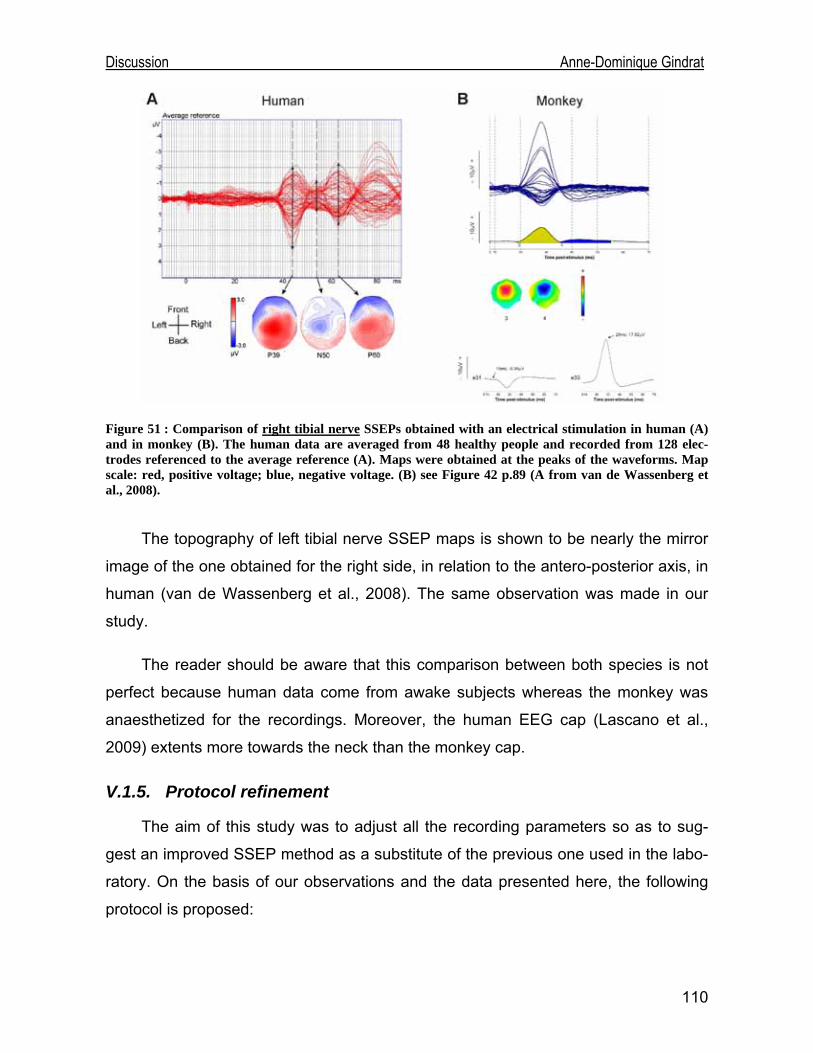
Discussion Anne-Dominique Gindrat
Figure 51 : Comparison of right tibial nerve SSEPs obtained with an electrical stimulation in human (A) and in monkey (B). The human data are averaged from 48 healthy people and recorded from 128 elec-trodes referenced to the average reference (A). Maps were obtained at the peaks of the waveforms. Map scale: red, positive voltage; blue, negative voltage. (B) see Figure 42 p.89 (A from van de Wassenberg et al., 2008).
The topography of left tibial nerve SSEP maps is shown to be nearly the mirror
image of the one obtained for the right side, in relation to the antero-posterior axis, in
human (van de Wassenberg et al., 2008). The same observation was made in our
study.
The reader should be aware that this comparison between both species is not
perfect because human data come from awake subjects whereas the monkey was
anaesthetized for the recordings. Moreover, the human EEG cap (Lascano et al.,
2009) extents more towards the neck than the monkey cap.
V.1.5. Protocol refinement
The aim of this study was to adjust all the recording parameters so as to sug-
gest an improved SSEP method as a substitute of the previous one used in the labo-
ratory. On the basis of our observations and the data presented here, the following
protocol is proposed:
110
Discussion Anne-Dominique Gindrat
Before recording SSEPs, it is required to shave off the scalp of the monkey and
to clean it with alcohol in order to obtain much lower electrode impedance. Indeed,
some recordings were performed without this preliminary step and it appeared that it
was much more difficult to obtain low electrode impedance and therefore, the re-
sponses were more contaminated by electrical noise. Moreover, to avoid noise as
much as possible, we recommend that the recordings are performed in a Faraday
room.
The electrode impedance determines the quality of the recorded signal. There-
fore, it is important to keep it as low as possible to perform the recordings. We rec-
ommend to check it regularly during the recordings and to adjust it if necessary by
applying some supplementary conductive past. Nevertheless, in the course of time,
electrode surface become oxidized and must be cleaned. If it is not possible, elec-
trodes must be replaced.
The room temperature and/or the animal temperature must be checked because
it is possible that it induces latency variations in the responses.
The best stimulation parameters are 0.5Hz frequency and slightly supra-liminar
intensity, allowing to obtain responses with the largest amplitude. Furthermore, the
stimulation sites should be beforehand shaved off and cleaned with alcohol to obtain
as best stimulation effect as possible.
We showed that sevoflurane anaesthesia was of prime choice as regards to the
stability and reproducibility of the responses as well as for the comfort of the animal.
Moreover, one should try to find the lowest concentration that allows to maintain the
animal in a stable state. If gas concentration is changed during the session, one must
wait for a while (15 minutes minimum for median nerve SSEPs) before performing
new acquisitions, so as to allow the gas concentration to balance.
In optimal conditions, without noise, 2 minutes 30s recordings (75 sweeps) are
sufficient to obtain a clear response. Nevertheless, if there is electrical noise, longer
acquisitions are required because some sweeps must be rejected.
111
Discussion Anne-Dominique Gindrat
The median nerve SSEPs should be preferred because responses were not as
contaminated by noise as tibial nerve SSEPs, as already previously reported in hu-
man.
V.1.6. Advantages of multichannel SSEP recordings over previous techniques
Epidural SSEP recordings were performed previously in the laboratory to inves-
tigate the functional recovery following a cortical lesion (Kaeser et al., 2006, 2007)
but this method had limitations. Moreover, surface SSEP recordings with the minimal
recommended montage of four channels (American Clinical Neurophysiology Soci-
ety, 2006) have limitations too. Therefore, at the cost of some additional preparation
time, the simple approach presented in this report has been developed and offers
several advantages over previous SSEP recording techniques:
First, our method is only minimally invasive, what constitutes an obvious advan-
tage as compared to epidural SSEP recordings. Consequently, acquisitions can be
performed more frequently. This allows to study the same animal over the long term,
what will be useful in the future to follow the time course of the recovery after a le-
sion. Moreover, given that the same animal can be studied for a long time, the vari-
ability decreases.
Second, the EEG cap covers the whole scalp. Therefore, recordings are not lim-
ited to a small region, as in the case of epidural recordings, and large-scale neuronal
networks can be investigated with a high temporal resolution, although the spatial
resolution of SSEPs is low. It means that it will be possible to follow the post-lesional
reorganization also in the intact hemisphere, what is interesting because the exact
role of contralesional areas in the recovery is not well known in monkeys (Rouiller
and Olivier, 2004).
Third, our method provides much more reproducible responses than the epidu-
ral SSEP technique of the laboratory with which it was difficult to obtain a stable pre-
lesional baseline for the amplitude and latency of the components (Gindrat, 2008). It
makes the new approach appropriate for long-term assessment of the brain activity.
112
Discussion Anne-Dominique Gindrat
Fourth, as demonstrated by van de Wassenberg et al. (2007, 2008), the high-
resolution SSEP method can measure median and tibial nerve SSEP amplitude more
accurately and consequently may be more sensitive to physiological and pathological
changes than classical recordings with a minimal montage. Indeed, the more chan-
nels are used, the more inter-individual variability in amplitude due to differences in
generator orientation will decrease.
Last but not least, high-resolution scalp SSEPs allow to build topographical
SSEP maps to study the spatio-temporal extent of the different electrical fields at the
scalp. Moreover, the position and strength of the electrical sources associated with
scalp recorded SSEPs can be determined using source location algorithms (Michel et
al., 1999; 2001; 2004).
In sum, despite their quite low spatial resolution due to the distance between the
scalp electrodes and neural generators, multichannel SSEPs represent an interesting
approach. If one wants to observe some spatial aspects in more detail, SSEP re-
cordings should be associated with higher spatial resolution techniques, such as the
MRI or fMRI.
V.2. Behavioural data
The hand dominance and preference of our animal were first studied by Pauline
Chatagny (2009) on a 27 days period. As far as the unimanual Brinkman task is con-
cerned, she did not observe any hand dominance in each slot type, whereas in this
study the animal showed a left hand dominance in vertical slots and a right hand
dominance in horizontal ones, but no dominance if all slots were considered (Figure 44). On the other hand, she observed a right hand preference in each slot type when
both hands could be used together, whereas no hand preference was detected in our
study (Figure 45). These discrepancies are probably due to the small number of
sessions considered in the study of Pauline Chatagny, with the monkey naive at the
beginning of the task and therefore in the learning phase. Therefore, it will be rele-
vant in the future to confirm our dominance/preference results by calculating the con-
tact time in the slots for each hand. Moreover, the results of the other dexterity tasks
113

Discussion Anne-Dominique Gindrat
114
will be interesting. Indeed, the monkey is better with the right hand than with the left
one for the drawer task, suggesting a task-specific hand dominance.
In the unimanual Brinkman task performed with the right hand, the monkey was
significantly better in 30s to retrieve pellets from the horizontal slots than from the
vertical ones (p<0.0001, paired t-test). The same phenomenon appeared in the bi-
manual Brinkman task with the left hand (p=0.0216, paired t-test). It is quite surpris-
ing because grasping from the horizontal slots requires an additional rotation of the
wrist as compared to reaching from the vertical slots (Freund et al., 2009) and is con-
sequently more complex. The inverse situation would be rather expected.
It emerges from the Brinkman task that the score in 30s of each hand is higher
when the task is performed unimanually than bimanually. This is coherent because in
this first situation, the working hand of the animal is not hampered with the other
hand.
We mentioned that the performance of the left hand was less constant than the
one of the right hand in the unimanual Brinkman task. This is probably due to a lack
of motivation rather than a real incapacity to perform the task, given that the score
can increase or decrease a lot from one session to the other, meaning that the ani-
mal is able to perform the task but does not always want. Some noise or some irrita-
bility the day after an anaesthesia can also explain in part the fluctuations of the re-
sults. The performance of the right hand in the drawer task decreased in the last ses-
sions, visible mainly with the increased load force and the picking time, probably for
the same reasons.
For the moment, it is quite difficult to interpret the drawer task data given that
the performance of the animal is not extremely stable yet, especially if one considers
the load force score for the right hand (Figure 47). Some supplementary training is
required. Moreover, only few data are available for other animals in the laboratory.
Discussion Anne-Dominique Gindrat
V.3. Prospects
The results exposed here constitute the first step of the project. They show that
our SSEP recording method is valid. We expect that functional recovery following a
cortical lesion implicates plastic mechanisms in the brain which can be investigated
and better understood with SSEPs. We are confident that this approach will be rele-
vant in the future to evaluate the extent of the cortical lesion before performing histo-
logical study and to follow in time the possible cortical reorganization in the acute
phase as well as in the recovery phase. In this case, this approach would have a
prognostic value for the recovery, as it is already the case in human (see for example
Carter and Butt, 2005). This study will continue in the following way:
The present study is based only on one animal. It was sufficient to develop the
cap and fix the different recording parameters. However, it is obvious that the inter-
individual stability of the evoked responses remains to be tested. Therefore, the ani-
mal of this study and probably three other ones will be included in a cortical lesion
protocol. They will follow a pre-lesional training for the behavioural tasks, as ex-
plained in this study, and once their performances will become stable, the animals
will undergo a cortical lesion. The first two animals will be control subjects, and the
last two will receive a treatment. Post-lesional SSEP recordings will be performed al-
lowing to follow in time a possible cortical reorganization from a topographical point
of view. In parallel, behavioural tests will continue in order to study if functional re-
covery follows the same time course as SSEP topographical modifications.
Until now, suppositions only have been made about the location and orientation
of the generators (see section V.1.3 of the discussion). In the future, on the basis of
our multichannel SSEP recordings and MRI data, we will try to estimate the location
of the most probable neural sources in the brain using an inverse solution algorithm
(Michel et al., 1999, 2001, 2004). Classically, the generators were investigated in
monkeys using invasive recordings on the surface of the cortex or directly into the
cortex (Allison et al., 1991a, 1991b; Arezzo et al., 1979, 1981; McCarthy et al., 1991)
but recently, the method of inverse solution, already used in human (Michel et al.,
115
Discussion Anne-Dominique Gindrat
116
1999, 2001, 2004), has been applied in monkeys too in order to explore spatio-
temporal patterns of neural activity (Fontanarosa et al., 2004).
In the present protocol, recordings were performed on an anaesthetized animal.
But as mentioned before, the goal is to perform recordings on a conscious animal. To
this aim, the monkey is trained daily to wear a cap during behavioural tasks. It will
however take a longer time before the animal accepts to wear a cap for a quite long
period. Of course the animal will be anaesthetized to install the EEG cap. Then it will
be woken up to perform the SSEP recordings. Meanwhile, it would be relevant to test
if it is possible to anaesthetize the animal directly at 1.5% sevoflurane after the induc-
tion of the anaesthesia to acquire SSEPs. This condition would be better for the ani-
mal if it remains well anaesthetized until the end of the recording session. It would be
interesting to see if there are topographical changes between SSEPs acquired at
deep and light anaesthesia, as shown in rodents (Mégevand et al., 2008).
Conclusion Anne-Dominique Gindrat
VI. Conclusion The present study confirms that SSEPs can be successfully recorded from a
multichannel EEG cap in macaque monkey. The major advantages of this method
are its minimally invasive nature, its simplicity, its high temporal resolution, the possi-
bility to record at the whole scalp, and the response stability. However, only a very
limited number of studies report multichannel EPs recorded in monkey (Fontanarosa
et al., 2004). On the basis of the diagnostic value of the high-resolution EP method
already known in human (see for example Lascano et al., 2009; van de Wassenberg
et al., 2008a and b), our technique could have an interesting value nowadays where
one looks for non-invasive methods also in animal research. Moreover, this approach
could be complemented with higher spatial resolution techniques, such as MRI or
fMRI, to assess the cortical activity over the long term.
117
References Anne-Dominique Gindrat
VII. References Accadbleb F., Henry P., de Gauzy J.S., Cahuzac J.P. (2006), Spinal Cord Monitoring in Scoliosis Surgery Using an Epidural Electrode. Results of a Prospective, Consecutive Series of 191 Cases, Spine 31(22): 2614–2623. Adrian, E.D. (1936), The Electrical Activity of the Cortex, Proc. R. Soc. Med. 29(3): 197–200. Adrian E.D. (1941), Afferent discharges to the cerebral cortex from peripheral sense organs, J. Physiol. 100: 159-191. Allison T., McCarthy G., Wood C.C., Darcey T.M., Spencer D.D, Williamson P.D. (1989a), Human Cortical Potentials Evoked by Stimulation of the Median Nerve. I. Cytoarchitectonic Areas Generating Short-Latency Activity, J. Neurophysiol. 62(3): 694-710. Allison T., McCarthy G., Wood C.C., Jones S.J. (1991a), Potentials evoked in human and monkey cerebral cortex by stimula-tion of the median nerve, Brain 114: 2465-2503. Allison T., McCarthy G., Wood C.C, Williamson P.D., Spencer D.D (1989b), Human Cortical Potentials Evoked by Stimula-tion of the Median Nerve. II. Cytoarchitectonic Areas Generating Long-Latency Activity, J. Neurophysiol. 62(3): 711-722. Allison T., Wood C.C., McCarthy G., Spencer D.D. (1991b), Cortical Somatosensory Evoked Potentials. II. Effects of Exci-sion of Somatosensory or Motor Cortex in Human and Monkeys, J. Neurophysiol. 66(1): 64-82. American Clinical Neurophysiology Society (2006), Guideline 9D: Guidelines on short-latency somatosensory evoked poten-tials, J Clin Neurophysiol. 23: 168–79. Aminoff M.J., Eisen A.A. (1998), AAEM minimonograph 19: Somatosensory evoked potentials, Muscle nerve 21: 277-290. Araki A., Takasa A., Yasuhara A., Kobayashi Y. (1999), The effect of stimulus rates on the amplitude of median nerve soma-tosensory evoked potentials: the developmental change, Brain and Development 21: 118-121. Arezzo J., Legatt A.D., Vaughan H.G., Jr. (1979), Topography and intracranial sources of somatosensory evoked potentials in the monkey. I. Early components, Electroencephalogr. Clin. Neurophysiol. 46(2): 155-72. Arezzo J.C., Vaughan H.G., Jr., Legatt A.D. (1981), Topography and intracranial sources of somatosensory evoked poten-tials in the monkey. II. Cortical components, Electroencephalogr. Clin. Neurophysiol. 51(1): 1-18. Asanuma H., Rosén I. (1972), Topographical organization of cortical efferent zones projecting to distal forelimb muscles in the monkey, Exp. Brain Res. 14: 243-256. Astle, D.E., Nobre A.C., Scerif G. (2009), Applying an Attentional Set to Perceived and Remembered Feaures, PloS ONE 4(10): e7613. Avery R.A., Franowicz J.S., Studholme C., van Dyck C.H., Arnsten A.F.T. (2000), The alpha-2A-adrenoceptor agonist, guan-facine, increases regional cerebral blood flow in dorsolateral prefrontal cortex of monkeys performing a spatial working memory task, Neuropsychopharmacology 23(3): 240-249. Banoub M., Tetzlaff J.E., Schubert A. (2003), Pharmacologic and Physiologic Influences Affecting Sensory Evoked Poten-tials: Implications for Perioperative Monitoring, Anesthesiology 99: 716–37. Bear M.F., Connors B.W., Paradiso M.A. (2006), Neuroscience: exploring the brain, 3rd edition, Lippincott Williams & Wilkins, 23-48, 387-421, 586-593. Beaud M.-L. (2007), Histological, behavioural and electrophysiological study of functional recovery in adult monkeys sub-jected to lesion of the spinal cord, Master thesis, University of Fribourg.
118

References Anne-Dominique Gindrat
Berger J.R., Blum A.S., Somatosensory Evoked Potentials, in: Blum A.S., Rutkove S.B. (2007), The Clinical Neurophysiology Primer, Humana Press Totowa, New Jersey. Berthet J. (2006), Dictionnaire de Biologie, Edition De Boeck Université, 712. Blaizot X., Landeau B., Baron J.-C., Chavoix C. (2000), Mapping the Visual Recognition Memory Network With PET in the Behaving Baboon, Journal of Cerebral Blood Flow & Metabolism 20: 213–219. Boisseau N., Madany M., Staccini P., Armando G., Martin F., Grimaud D., Raucoules-Aimé M. (2002), Comparison of the effect of sevoflurane and propofol on cortical somatosensory evoked potentials, Br. J. Anaesth. 88: 785-789. Bonadio, C. (2000), Macaca fascicularis (On-line), Animal Diversity Web. http://animaldiversity.ummz.umich.edu/site/accounts/information/Macaca_fascicularis.html. Bremer F, Dow R.S. (1939), The cerebral acoustic area of the cat: a combined oscillographic and cytoarchitectonic study, J. Neurophysiol. 2: 308-318. Brinkman C. (1984), Supplementary motor area of the monkey's cerebral cortex: short- and long-term deficits after unilateral ablation and the effects of subsequent callosal section, J. Neurosci. 4: 918-29. Brinkman J., Kuypers H.G.J.M. (1973), Cerebral control of contralateral and ipsilateral arm, hand and finger movements in the split-brain rhesus monkey, Brain 96: 653-74. Burghaus L., Lui W.-C., Dohmen C., Bosche B., Haupt W.F. (2008), Evoked Potentials in Acute Stroke within the First 24h : Possible Predictor of a Malignant Course, Neurocrit. Care 9: 13-16. Buzsáki G. (2004), Large-scale recording of neuronal ensembles, Nat. Neurosci. 7: 446-451. Carter B.G., Butt W. (2001), Review of the use of somatosensory evoked potentials in the prediction of outcome after severe brain injury, Crit. Care Med. 29(1): 178-186. Carter B.G., Butt W. (2005), Are somatosensory evoked potentials the best predictor of outcome after severe brain injury? A systematic review, Intensive Care Med. 31: 765-775. Carter B.G., Taylor A., Butt W. (1999), Severe brain injury in children: long-term outcome and its prediction using somato-sensory evoked potentials (SEPs), Intensive Care Med. 25: 722-728. Cartool Reference Guide (http://brainmapping.unige.ch/cartool/refguide/cartool.html). Caton R. (1875), The Electric Currents of the Brain, Br. Med. J. 2: 278. Chatagny P. (2009), Etude de la dominance et de la préférence manuelles chez le macaque à longue queue (Macaca fasci-cularis), Bachelor thesis, University of Fribourg. Cohen A. R.; Young W.; Ransohoff J. (1981), Intraspinal localization of the somatosensory evoked potential, Neurosurgery 9(2): 157-162 (abstract only). Cohen of Birkenhead (1959), Richard Caton (1842-1926) Pioneer Electrophysiologist, Proc. R. Soc. Med. 52(8): 645–651. Coles, M.G.H.; Rugg M. D. (1996), Event-related brain potentials an introduction, in: Electrophysiology of Mind. Oxford Scholarship Online Monographs. 1–27. Cracco J.B. (1989), Somatosensory Evoked Potentials in Infants and Children, J. Child Neurol. 4: 2, 70-72. Cruccu G., Aminoff M.J., Curio G., Guerit J.M., Kakigi R., Mauguière F., Rossini P.M., Treede R.-D., Garcia-Larrea L (2008), Recommendations for the clinical use of somatosensory-evoked potentials, Clin. Neurophysiol. 119(8): 1705-1719.
119

References Anne-Dominique Gindrat
Cusick J.F.; Myklebust J.B.; Larson S.J.; Sances A. (1979), Spinal cord evaluation by cortical evoked responses, Arch. Neu-rol. 36(3): 140-143 (abstract only). Dawson G.D. (1947a), Cerebral responses to electrical stimulation of peripheral nerve in human, J. Neurol. Neurosurg. Psy-chiatry 10(3): 134–140. Dawson G.D (1947b), Investigations on a patient subject to myoclonic seizures after sensory stimulation, J. Neurol. Neuro-surg. Psychiatry 10(4): 141–162. Desmedt J.E. (1987), Physiologie et physiopathologie des sensations somatiques étudiées chez l’Homme par la méthode des potentiels évoqués, Journal de Physiologie 82(2): 64-136. Detsch O., Kochs E. (1997), Effekte von Ketamin auf die ZNS-Funktion, Anaesthesist [Suppl 1] 46: S20-S29. Dunn A.K., Bolay T., Moskowitz M.A., Boas D.A. (2001), Dynamic Imaging of Cerebral Blood Flow Using Laser Speckle, J. Cereb. Blood Flow Metab. 21(3): 195–201. Durduran T., Burnett M.G., Yu G., Zhou C., Furuy D., Yod, A.G., Detre J.A.; Greenburg J.H. (2004), Spatiotemporal quantifi-cation of cerebral blood flow during functional activation in rat somatosensory cortex using laser-speckle flowmetry, J. Cereb. Blood Flow Metab. 24: 518–525. Erwin C.W., Rozear M.P., Radtke R.A., Erwin A.C., Somatosensory evoked potentials, in Niedermeyer E., Lopes da Silva F.H. (1987), Electroencephalography: Basic Principles, Clinical Applications and Related Fields, second edition, Urban & Schwarzenberg, 817-833. Feys H., Van Hees J., Bruyninckx F., Mercelis R., De Weerdt W. (2000), Value of somatosensory and motor evoked poten-tials in predicting arm recovery after a stroke, J. Neurol. Neurosurg. Psychiatry 68:323–331. Fontanarosa JB, Lasky RE, Lee HC, van Drongelen W. (2004), Localization of Brain stem Auditory Evoked Potentials in Primates: A Comparison of Localization Techniques Applied to Deep Brain Sources, Brain Topogr. 17(2): 99-108. Freund, P., Schmidlin, E., Wannier, T., Bloch, J., Mir, A., Schwab, M.E., Rouiller, E.M. (2009), Anti-Nogo-A antibody treat-ment promotes recovery of manual dexterity after unilateral cervical lesion in adult primates--re-examination and extension of behavioral data, Eur. J. Neurosci. 29: 983-996. Freye E. (2005), Cerebral monitoring in the operating room and the intensive care unit – an introductory for the clinician and a guide for the novice wanting to open a window to the brain, II. Sensory-Evoked Potentials (SSEP, AEP, VEP), Journal of Clinical Monitoring and Computing 19: 77–168. Geselowitz D.B. (1998), The zero of potential, IEEE Eng. Med. Biol. Mag. 17(1): 132. Gilmore R. (1989), The Use of Somatosensory Evoked Potentials in Infants and Children, J. Child Neurol. 4: 3-19. Giesser B.S. (1993), Evoked Potentials As Outcome Measures in Multiple Sclerosis, J. Neuro. Rehab. 7: 99-104. Gindrat A.-D. (2008), Évolution de la performance motrice fine, des potentiels évoqués somatosensoriels et des réponses aux microstimulations intracorticales chez le macaque à longue queue suite à une lésion du cortex moteur primaire, Bache-lor work, University of Fribourg. Gonzalez A.A., Jeyanandarajan D., Hansen C., Zada G., and Hsieh P.C. (2009), Intraoperative neurophysiological monitor-ing during spine surgery: a review, Neurosurg. Focus 27(4): E6. Gott P.S., Karnaze D.S., Fisher M. (1990), Assessment of median nerve somatosensory evoked potentials in cerebral ischemia, Stroke 21(8): 1167-71. Gray H. (1918), Anatomy of the Human Body, http://bartleby.com/.
120

References Anne-Dominique Gindrat
Gronseth G.S., Ashman E.J. (2000), Practice parameter: The usefulness of evoked potentials in identifying clinically silent lesions in patients with suspected multiple sclerosis (an evidence-based review). Report of the Quality Standards Subcom-mittee of the American Academy of Neurology, Neurology 54(9): 1720-5. Haas L (2003); Hans Berger (1873–1941), Richard Caton (1842–1926), and electroencephalography; J. Neurol. Neurosurg. Psychiatry. 74(1): 9. Hecht N., Woitzik J., Dreier J.P., Vajkoczy P. (2009), Intraoperative monitoring of cerebral blood flow by laser speckle con-trast analysis, Neurosurg. Focus 27(4): E11. Holmes G.L, Khazipov R, Basic Neurophysiology and the Cortical Basis of EEG, in: Blum A.S., Rutkove S.B. (2007),The Clinical Neurophysiology Primer, Humana Press Totowa, New Jersey. Jacobs A.H, Li H., Winkeler A., Hilker R., Knoess C., Rüger A., Galldiks N., Schaller B., Sobesky J., Kracht L., Monfared P., Klein M., Vollmar S., Bauer B., Wagner R., Graf R., Wienhard K., Herholz K., Heiss W.D. (2003), PET-based molecular im-aging in neuroscience, Eur. J. Nucl .Med. Mol. Imaging 30(7): 1051-1065. Kaeser M., Wannier T., Bloch J., Debatisse D., Pralong E., Brunet J.-F., Rouiller E.M., Cortical parallels functional recovery of manual dexterity after lesion of motor cortex in monkeys: long-term neuro-monitoring by using ECoG, poster presented at the 28th International Congress of Clinical Neurophysiology, Edinburgh, 2006. Kaeser M., Wannier T., Wyss A.F., Belhaj-Saïf A., Bloch J., Brunet J.-F., Debatisse D., Pralong E., Rouiller E.M., Cortical plasticity assessed by somatosensory evoked potentials (SEPs) parallels functional recovery of manual dexterity after lesion of primary motor cortex (M1) in monkeys, poster presented at the Swiss Society for Neuroscience meeting, Bern, 2007. Kahle W., Frotscher M. (2007), Atlas de poche d’anatomie, 3- Système nerveux et organes des sens, 4e édition, Médecine-Sciences Flammarion. Kallmann B.A., Fackelmann S., Toyka K.V., Rieckermann P., Reiners K. (2006), Early abnormalities of evoked potentials and future disability in patients with multiple sclerosis, Mult. Scler. 12: 58-65. Kandel E.R, Schwartz J.H , Jessel T.M. (2000), Principles of Neural Science, 4th edition, McGraw-Hill Health professions division New-York, 22, 430-450. Kazennikov O, Hyland B, Corboz M., Babalian A., Rouiller E.M., Wiesendanger M. (1999), Neural activity of supplementary and primary motor areas in monkeys and its relation to bimanual and unimanual movement sequences, Neuroscience 89: 661–674. Kazennikov O., Hyland B., Wicki U., Perrig S., Rouiller E.M., Wiesendanger M. (1998), Effects of lesions in the mesial frontal cortex on bimanual co-ordination in monkeys, Neuroscience 85: 703-716. Kazennikov O., Wicki U., Corboz M., Hyland B., Palmeri A., Rouiller E. M., Wiesendanger M (1994), Temporal structure of a bimanual goal-directed movement sequence in monkeys, Eur. J. Neurosci. 6: 203-210. Keren O., Ring H., Solzi P., Pratt H., Groswasser Z. (1993), Upper limb somatosensory evoked potentials as a predictor of rehabilitation progress in dominant hemisphere stroke patients, Stroke 24(12): 1789-1793. Kermadi I., Liu Y., Tempini A., Calciati E., Rouiller E. M. (1998), Neuronal activity in the primate supplementary motor area and the primary motor cortex in relation to spatio-temporal bimanual coordination, Somatosens. Mot. Res. 15: 287-308. Kermadi I., Liu Y., Tempini A., Rouiller E. M. (1997), Effects of reversible inactivation of the supplementary motor area (SMA) on unimanual grasp and bimanual pull and grasp performance in monkeys, Somatosens. Mot. Res. 14: 268-280. Kermadi I., Liu Y., Tempini A., Rouiller E. M. (2000), Do bimanual motor actions involve the dorsal premotor (PMd), cingulate (CMA) and posterior parietal (PPC) cortices? Comparison with primary and supplementary motor cortical areas, Somato-sens. Mot. Res. 17: 255-271.
121
References Anne-Dominique Gindrat
Lascano A.M., Brodbeck V., Lalive P.H., Chofflon M., Seeck M., Michel C.M. (2009), Increasing the Diagnostic Value of Evoked Potentials in Multiple Sclerosis by Quantitative Topographic Analysis of Multichannel Recordings, J. Clin. Neuro-physiol. 26(5): 316-325. Legatt A. D., Soliman E. (2006), Somatosensory Evoked Potentials: General Principles, http://emedicine.medscape.com/article/1139906-overview. Lew H.L., Dikmen S., Slimp J., Temkin N., Lee E.H., Newell D., Robinson L.R. (2003), Use of somatosensory-evoked poten-tials and cognitive event-related potentials in predicting outcomes of patients with severe traumatic brain injury, Am. J. Phys. Med. Rehabil. 82(1): 53-61. Liu Y, Rouiller E.M. (1999), Mechanisms of recovery of dexterity following unilateral lesion of the sensorimotor cortex in adult monkeys, Exp. Brain Res. 128: 149-159. McCarthy G., Wood C.C., Allison T. (1991), Cortical Somatosensory Evoked Potentials. I. Recordings in the Monkey Macaca fascicularis, J. Neurophysiol. 66(1): 53-63. Machado C., Early prediction of the clinical course in cerebrovascular coma by evoked potentials, in: Kimura J., Shibasaki H. (1996), Recent Advances in Clinical Neurophysiology : Proceedings of the Xth International Congress of EMG and Clinical Neurophysiology, Kyoto, Japan, 15-19 October 1995 (International Congress Series), Elsevier Science B.V. Malmivuo J., Plonsey R. (1995), Bioelectromagnetism - Principles and Applications of Bioelectric and Biomagnetic Fields, Oxford University Press, chapter 13, webversion : http://www.bem.fi/book/index.htm. Mani A., Absalom V (2006), Advanced neurological monitoring, Surgery 24(10): 337-340. Marshall W.H., Woolsey C.N., Bard P. (1941), Observations on cortical somatic sensory mechanisms of cat and monkey, J. Neurophysiol. 4(1): 1–24. Mauguière F., Somatosensory Evoked Potentials :Normal Responses, Abnormal Waveforms, and Clinical Applications in Neurological Diseases, in Niedermeyer E., Lopes da Silva F.H. (2005), Electroencephalography: Basic Principles, Clinical Applications and Related Fields, fifth edition Philadelphia : Lippincott Williams & Wilkins, 1067-1119. Mauguière F., Fischer C. (4-1990), Les potentiels évoqués en neurologie, Editions Techniques, Encycl. Méd. Chir. (Paris-France), Neurologie, 17031B10, 26p. Mégevand P., Quairiaux C, Lascano A.M., Kiss J.K, Michel C.M. (2008), A mouse model for studying large-scale neuronal networks using EEG mapping techniques. NeuroImage 42: 591-602, doi:10.1016/j.neuroimage.2008.05.016. Michel, C.M., Murray, M.M., Lantz, G., Gonzalez, S., Spinelli, L., Grave de Peralta, R. (2004), EEG source imaging, Clin. Neurophysiol. 115: 2195–2222. Michel C.M., Seeck M., Landis T. (1999), Spatiotemporal Dynamics of Human Cognition, News Physiol. Sci. 14: 206-214. Michel, C.M., Thut, G., Morand, S., Khateb, A., Pegna, A.J., Grave de Peralta, R., Gonzalez, S., Seeck, M., Landis, T. (2001), Electric source imaging of human brain functions, Brain Res. Brain Res. Rev. 36: 108–118. Murray, M.M., Brunet, D., Michel, C.M. (2008), Topographic ERP Analyses: a step-by-step tutorial review, Brain Topogr. 20: 249–264. Napier J.R. (1956), The prehensile movements of the human hand, The journal of bone and joint surgery 38-B(4): 902-13. Netter F.H., Craig J.A., Perkins J., Hansen J.T., Koeppen B.M. (2002), Atlas of Neuroanatomy and Neurophysiology, Selec-tions from the Netter Collection of Medical Illustrations, Icon Custom Communications.
122

References Anne-Dominique Gindrat
Ormerod W. (2006), Richard Caton (1842-1926): pioneer electrophysiologist and cardiologist, Journal of Medical Biography, 14: 30-35. Panayiotopoulos C.P. (2005), The epilepsies: Seizures, Syndromes and Management, 1st edition, Bladon Medical Publish-ing, 45-58. Pascual-Marqui, R.D., Michel, C.M., Lehmann, D. (1995), Segmentation of brain electrical activity into microstates: model estimation and validation. IEEE Trans. Biomed. Eng. 42: 658–665. Penfield W.G., Boldrey E. (1937), Somatic motor and sensory representation in the cerebral cortex of man as studied by electrical stimulation, Brain 60: 389-443. Prestor B., Gnidovec B., Golob P. (1997), Long sensory tracts (cuneate fascicle) in cervical somatosensory evoked potential after median nerve stimulation, Electroencephalogr. Clin. Neurophysiol. 104(6): 470–479. Purves D, Augustine G.J., Fitzpatrick D., Hall W.C, LaMantia A.-S., McNamara J.O., Williams S.M. (2004), Neuroscience, 3rd edition, Sinauer Associates, Inc. 26-27, 189-228, 668-670. Quairiaux C., Armstrong-James M., Welker E. (2007), Modified Sensory Processing in the Barrel Cortex of the Adult Mouse After Chronic Whisker Stimulation, J. Neurophysiol. 97: 2130-2147. Regan D. (1989), Human Brain Electrophysiology: Evoked Potentials and Evoked Magnetic Fields in Science and Medicine, Elsevier Science Ltd, 498-507. Rehberg B., Rüschner R., Fischer M., Ebeling B.J., Hoeft A. (1998), Konzentrationsabhängige Veränderungen der Latenz und Amplitude somatosensorisch evozierter Potentiale durch Desflurane, Isoflurane und Sevoflurane, Anasthesiol. Inten-sivmed. Notfallmed. Schmerzther. 33(7): 425-9. Rouiller E.M., Olivier E. (2004), Functional recovery after lesions of the primary motor cortex, Progress in Brain Research 143:467-475. Rouiller E.M., Yu X.H., Moret V., Tempini A., Wiesendanger M., Liang F. (1998), Dexterity in adult monkeys following early lesion of the motor cortical hand area : the role of cortex adjacent to the lesion, Eur. J. Neurosci. 10: 729-40. Sanei S., Chambers J.A. (2007), EEG Signal Processing, John Wiley & Sons Ltd, 1-4, 15-17. Schmidlin E., Wannier T., Bloch J., Belhaj-Saïf A., Wyss A.F., Rouiller E.M. (2005), Reduction of the hand representation in the ipsilateral primary motor cortex following unilateral section of the corticospinal tract at cervical level in monkeys, BMC Neuroscience 6: 56. Schmidlin E., Wannier T., Bloch J., Rouiller E.M. (2004), Progressive plastic changes in the hand representation of the pri-mary motor cortex parallel incomplete recovery from a unilateral section of the corticospinal tract at cervical level in monkeys, Brain Research 1017: 172-183. Schwender D., End H., Daunderer M., Fiedermutz M., Peter K. (1998), Sevofluran und Nervensystem, Anaesthesist [Suppl 1] 47: S37-S42. Sessle B.J., Wiesendanger M. (1982), Structural and functional definition of the motor cortex in the monkey (Macaca fascicu-laris), J. Physiol. 323: 245-265. ShagassC., Schwartz M., Age, Personality, and Somatosensory Cerebral Evoked Responses, Science 148: 1359-1351. Speckmann E.-J., Elger C.E., Introduction to the Neurophysiological Basis of the EEG and DC Potentials, in Niedermeyer E., Lopes da Silva F.H. (1987), Electroencephalography: Basic Principles, Clinical Applications and Related Fields, second edi-tion, Urban & Schwarzenberg, 817-833.
123
References Anne-Dominique Gindrat
Stefanacci L., Reber P., Costanza J., Wong E., Buxton R., Zola S., Squire L., Albright T. (1998), fMRI of Monkey Visual Cor-tex, Neuron 20: 1051-1057. Stienen P.J., Haberham Z.L., van den Brom W.E., de Groot H.N.M., Venker-Van Haagen A.J., Hellebrekers L.J. (2003), Evaluation of methods for eliciting somatosensory-evoked potentials in the awake, freely moving rat, Journal of Neurosci-ence Methods 126: 79-/90. Tan Y.E., Lo Y.L. (2003), Intra-operative monitoring with somatosensory evoked potentials, SGH proceedings 12(1): 19-21. Tatsch K., Ell P.J. (2006), PET and SPECT in common neuropsychiatric disease, Clin. Med. 6: 259–62. Tibbo P., Silverstone P.H., Mc Ewan A.J.B., Scott J, Joshua A., Golberg K. (1996), A Single Photon Emission Computed Tomography Scan Study of Striatal Dopamine D2 Receptor Binding with l231-Epidepride in Patients with Schizophrenia and Controls, J. Psychiatry Neurosci. 22(1): 39-45. Troncoso E., Muller D., Czellar S., Kiss, J.Z. (2000), Epicranial sensory evoked potential recordings for repeated assessment of cortical functions in mice, Journal of Neuroscience Methods 97: 51–58. Umamaheswara Rao G.S. (2002), Neurological monitoring, J. Anaesth. 2002; 46(4): 304-314. van de Wassenberg W.J.G., van der Hoeven J.H., Leenders K.L., Maurits N.M. (2008a), Multichannel recording of median nerve somatosensory evoked potentials, Neurophysiol. Clin. 38(1): 9-21. van de Wassenberg W.J.G., Kruizinga W.J., van der Hoeven J.H., Leenders K.L., Maurits N.M. (2008b), Multichannel re-cording of tibial-nerve somatosensory evoked potentials, Neurophysiol. Clin. 38(5): 277-288. Vaughan D.J.A., Thornton C., Wright D.R., Fernandes J.R., Robbins P., Doré C., Brunner M.D. (2001), Effects of different concentrations of sevoflurane and desflurane on subcortical somatosensory evoked responses in anaesthetized, non-stimulated patients, Br. J. Anaest. 86(1): 59-62. Walsh P., Kane N., Butler S. (2005), The clinical role of evoked potentials, J. Neurol. Neurosurg. Psychiatry 76 (Suppl II): ii16–ii22. Walter W.G. (1937), The electroencephalogram in cases of cerebral tumour, Proc. Roy. Soc. Med. 30: 579-598. Wannier T., Liu J., Morel A, Jouffrais C., Rouiller E.M. (2002), Neuronal activity in primate striatum and pallidum related to bimanualmotor actions, NeuroReport 13(1): 143-147. Weber B., Burger C., Wyss M.T., von Schulthess G.K., Scheffold F., Buck A. (2004), Optical imaging of the spatiotemporal dynamics of cerebral blood flow and oxidative metabolism in the rat barrel cortex, Eur. J. Neurosci. 20(10): 2664-2670. Weiller C., May A., Sach M., Buhmann C., Rijntjes M. (2006), Role of Functional Imaging in Neurological Disorders, Journal of magnetic resonance imaging 23: 840-850. Wienbruch C., Candia V., Svensson J., Kleiser R., Kollias S.S. (2006), A portable and low-cost fMRI compatible pneumatic system for the investigation of the somatosensensory system in clinical and research environments, Neuroscience Letters 398: 183–188. Wyss A.F. (2007), Lesion of motor cortex in adult non-human primates: post-lesional plasticity and mechanisms of behavioral recovery, PhD thesis, University of Fribourg, Switzerland. Zeman B.D., Yiannikas C. (1989), Functional prognosis in stroke: use of somatosensory evoked potentials, J. Neurol. Neuro-surg. Psychiatry 52(2): 242-7. Zhou C., Shimazu T., Durduran T., Luckl J., Kimberg D.Y., Yu G., Chen X.H., Detre J.A., Yodh A.G., Greenberg J.H. (2008), Acute functional recovery of cerebral blood flow after forebrain ischemia in rat, J. Cereb. Blood Flow Metab. 28(7): 1275-84.
124

References Anne-Dominique Gindrat
125
Zumsteg D., Wieser H.G. (2002), Effects of aging and sex on middle-latency somatosensory evoked potentials: normative data, Clin. Neurophysiol. 113: 681-685. http://emedicine.medscape.com/article/1137763-overview, Accessed September 29, 2009. http://emedicine.medscape.com/article/1139906-overview, Accessed September 30, 2009. http://pin.primate.wisc.edu/factsheets/entry/long-tailed_macaque, Accessed September 22, 2009. http://pubpages.unh.edu/~jel/images/brain_glia.jpg, Accessed March 17, 2009. http://www.brainproducts.com/productdetails.php?id=29, Accessed January 16, 2010. http://www.egi.com/research-division-research-products/sensor-nets, Accessed October 05, 2009.

Appendixes Anne-Dominique Gindrat
VIII. Appendixes
Appendix 1: The median nerve
Figure 52 : Median nerve (from Netter et al., 2002, p. 44).
The median nerve (Figure 52) runs down the middle of the arm, the forearm, to the hand. It comes from two roots, one from the lateral and one from the medial cord of the brachial plexus, joining either in front of or lateral to the axillary artery. The median nerve fibres originate from roots from (C5, inconstant), C6, C7, C8 and T1 nerves. The nerve runs along the arm first lateral to the brachial artery; then it crosses this vessel at the level of the insertion of the M. Coraco-brachialis, and runs to the bend of the el-bow on the medial side of the artery. At that time, the nerve is located behind the lacer-tus fibrosus (bicipital fascia), and is sepa-rated from the elbow-joint by the M. Brachi-alis. In the elbow, it passes between the two
heads of the M. Pronator teres to enter in the forearm. It crosses the ulnar artery, but remains separated from this vessel by the deep head of the M. Pronator teres. Next, it passes between the M. Flexor digitorum superficialis and the M. Flexor digitorum profundus, and goes within 5 cm of the transverse carpal ligament (into the carpal tunnel). At this point, it is located more superficially, between the tendons of the M. Flexor digitorum superficialis and M. Flexor carpi radialis, on the radial side of the tendon of the M. Palmaris longus, where it is covered by the skin and the fascia. Subsequently, it runs behind the transversal carpal ligament to the palm of the hand.
This nerve innervates primarily the forearm (pronator and most of flexor muscles) and the palm of the hand (mo-tor innervation and palmar skin of the thumb, index, middle finger and half of the ring finger, Figure 52) by differ-ent branches (for further details, see Gray, 1918) (from Gray, 1918; Kahle and Frotsche, 2007, p. 76).
126

Appendixes Anne-Dominique Gindrat
Appendix 2: The tibial nerve
Figure 53 : Tibial nerve (from Netter et al., 2002, p. 49).
The tibial nerve (Figure 53) is the larger of the two terminal branches of the sciatic nerve. It comes from the ante-rior branches of the L4, L5, S1, S2 and S3 nerves. It runs down along the back of the thigh, under the M. gas-trocnemius, passes through the middle of the popliteal fossa, goes to the lower part of the M. Popliteus, and trav-els with the popliteal artery below the arch of the M. Soleus. Subsequently, it runs down along the back of the leg with the posterior tibial vessels, between the M. Flexor hallucis longus and the M. Flexor digitorum longus. Then, it goes down between the heel and the medial malleolus, parallel with the medial margin of the tendo calcaneus, and goes around the dorsal face of the medial malleolus. Finally, this nerve splits under the lacinate ligament into two terminal branches, namely the medial and the lateral plantar nerves.
The branches of this nerve are: articular, muscular, medial sural cutaneous, medial calcaneal, medial and lateral plantar (Figure 53). They innervate a part of the knee, the leg and the foot (for greater detail about the innerva-tion, see Gray, 1918) (from Gray, 1918; Kahle and Frotscher, 2007, p.94).
127
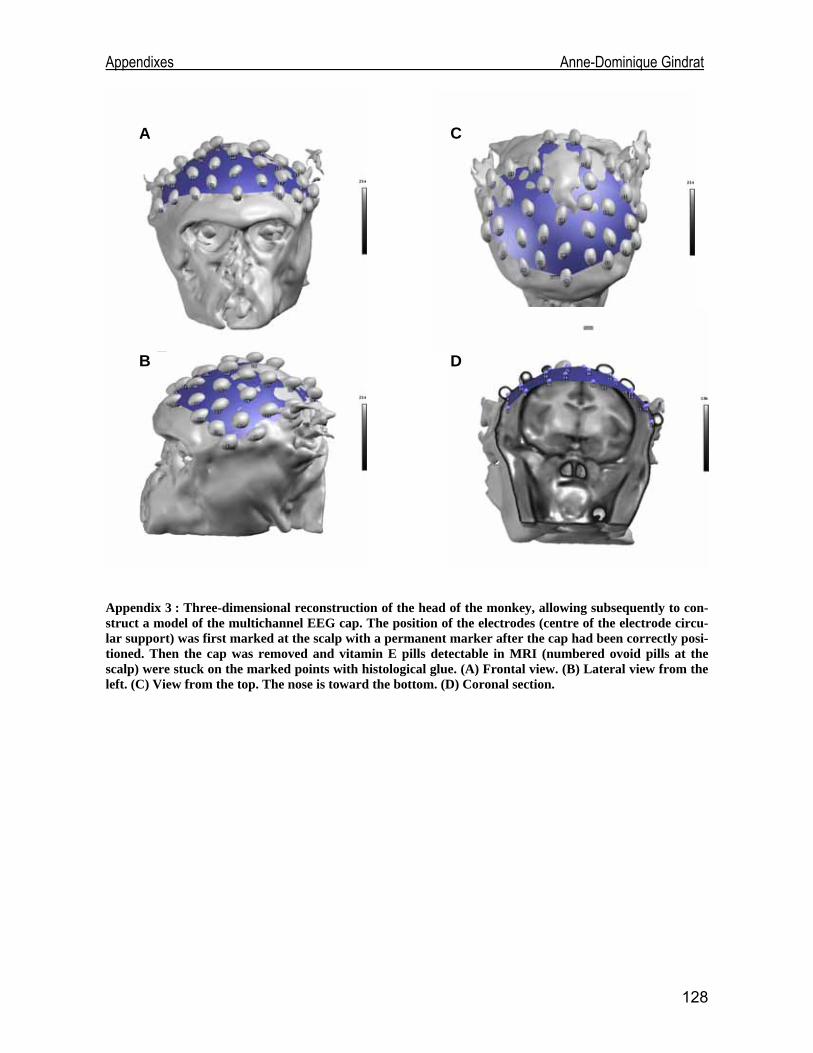
Appendixes Anne-Dominique Gindrat
A
B
C
D
Appendix 3 : Three-dimensional reconstruction of the head of the monkey, allowing subsequently to con-struct a model of the multichannel EEG cap. The position of the electrodes (centre of the electrode circu-lar support) was first marked at the scalp with a permanent marker after the cap had been correctly posi-tioned. Then the cap was removed and vitamin E pills detectable in MRI (numbered ovoid pills at the scalp) were stuck on the marked points with histological glue. (A) Frontal view. (B) Lateral view from the left. (C) View from the top. The nose is toward the bottom. (D) Coronal section.
128


