Development of an algorithm for estimating Lead-Acid ...830232/FULLTEXT01.pdf · Development of an...

1

Development of an algorithm for

estimating Lead-Acid Battery State of

Charge and State of Health.

Mateusz Michal Samolyk

Jakub Sobczak

This thesis is presented as part of Degree of

Master of Science in Electrical Engineering

Blekinge Institute of Technology

September 2013

Blekinge Institute of Technology

School of Engineering

Department of Electrical Engineering

Supervisor: Sen. Lec. Anders Hultgren

Examiner: Dr. Sven Johansson

3

Abstract – In this paper, a state of charge (SOC) and a state of health (SOH)

estimation method for lead-acid batteries are presented. In the algorithm the

measurements of battery’s terminal voltage, current and temperature are used in the

process of SOC calculation. The thesis was written in cooperation with Micropower AB.

The algorithm was designed to fulfill the specific requirements of the electric vehicles

application: an error below 5% of SOC, computational simplicity and the possibility of

being implemented in a basic programming languages. The current used method at

Micropower, Coulomb counting, is compared with a method presented by Chiasson and

Vairamohan 2005 based on modified Thevein circuit during charging and discharging of

the battery. The Thevenin based method gave better result compared to Coulomb

counting but seems not to fulfill Micropowers requirements. A correction method based

on periods of no charging or discharging, possible to be used together with Coulomb

counting as well as with the Thevenin method was developed. The evaluation method

indicates that when using also the correction method the Micropowers requirements are

fulfilled.

Keywords: : Lead-Acid Battery, SOC, SOH, Improved Coulomb Counting

5

Acknowledgments

We would like to thank our supervisor, Prof. Anders Hultgren for his time and support he has

provided us with during writing this thesis, Henrik Magnusson and the rest of the Micropower

AB staff for their advices and granting us the necessary equipment.

7

Table of Contents 1. Introduction ............................................................................................................................ 9

2. Theoretical Background ....................................................................................................... 11

2.1. Lead-Acid batteries ....................................................................................................... 11

2.1.1. Lead-Acid Battery structure, the principle of its operation .................................... 11

2.1.2. Electric model of the battery .................................................................................. 12

2.1.3. Lead-Acid battery types ......................................................................................... 14

2.1.4. Lead-acid batteries applications ............................................................................. 16

2.2. Other popular battery types and their applications ........................................................ 16

2.3. Battery variables ............................................................................................................ 17

2.4. Lead-Acid battery aging process ................................................................................... 19

2.5. State of charge monitoring methods for lead acid batteries .......................................... 20

2.5.1. Open circuit voltage method .................................................................................. 21

2.5.2. Specific Gravity (SG) method ................................................................................ 22

2.5.3. Coulomb counting method ..................................................................................... 22

2.5.4. Impedance measurement method ........................................................................... 23

2.6. Battery modeling techniques ......................................................................................... 23

2.7. Electric equivalent circuit models ................................................................................. 24

2.7.1. Simple battery model ............................................................................................. 24

2.7.2. Advanced simple battery model ............................................................................. 25

2.7.3. Thevenin battery model .......................................................................................... 25

2.7.4. Modified Thevenin Model ..................................................................................... 26

2.7.5. Third-Order Battery Model .................................................................................... 27

2.7.6. Simplified equivalent circuit model ................................................................... 28

3. Algorithm design and implementation ................................................................................. 29

3.1. Project requirements ...................................................................................................... 30

3.2. Reference method .......................................................................................................... 33

3.3. Designed method ........................................................................................................... 37

3.4. Laboratory setup ............................................................................................................ 44

3.5. Implementation .............................................................................................................. 47

3.5.1. Reference Method MatLab Implementation .......................................................... 47

3.5.2. Designed Algorithm MatLab Implementation ...................................................... 50

3.5.3. SOH estimation ...................................................................................................... 66

4. Tests ..................................................................................................................................... 69

8

4.1. Reference method .......................................................................................................... 69

4.2. Designed Algorithm ...................................................................................................... 74

5. Conclusions and future work ................................................................................................ 77

5.1. Conclusions ................................................................................................................... 77

5.2. Future work ................................................................................................................... 79

6. References ............................................................................................................................ 80

9

1. Introduction

Electricity plays a crucial role in everyone's life nowadays. It is used in a variety of

different devices with people accustomed to them too much to even notice how necessary

they became. However, with the tremendous technological progress in electronic industry

many challenges arise. Even though the Devices' performance is growing exponentially their

size is constantly minimized in order to satisfy the modern customer needs.

A decade ago mobility used to be a synonym of freedom, nowadays mobility is a

standard. With mobility being a requirement of electronic devices, there comes another one -

a need of a reliable mobile energy storage - a Battery. A battery for an Electric Vehicle is

equivalent to the fuel tank for a typical, gasoline car. Imagine a car without the fuel-level

indicator on the dashboard. Notice how inconvenient would it be for the driver not to have the

precise indicator of how many miles the car can still travel.

With the popularization of the Electric Vehicles and Hybrid-Electric Vehicles, such as

cars, forklifts and the wheelchairs there is a growing demand for a Battery State of Charge

indicator, a software or hardware designed to estimate the remaining effective capacity of the

battery having only the measurements of limited number of variables.

The aim of this paper is to cover the Lead-Acid battery State of Charge and State of

Health estimation problem and produce a viable solution in the form of algorithm, capable of

estimating those two states with a minimal input required from the operator.

The introduction to the topic and the theoretical background is included in the first two

chapters of this Thesis. The third one covers the project requirements, practical description of

the algorithm, its implementation and the laboratory setup. The fourth chapter includes the

data from the tests carried out in the laboratory and its comparison with the reference data as

well. The fifth one concludes the research and contains suggestions towards a future work in

the area of Battery State of Charge and State of Health estimation. The references are grouped

and described in the last chapter of this paper.

11

2. Theoretical Background

2.1. Lead-Acid batteries

2.1.1. Lead-Acid Battery structure, the principle of its operation

There are two main battery system categories, i.e.:

1. Batteries which convert their chemical energy into electrical only once (primary

cells)

2. Batteries which can convert chemical energy into electrical multiple times

(secondary cells)

The second type of batteries are much more practical than the primary type, as their

usage is by far more cost-efficient as it allows for long terms of use.

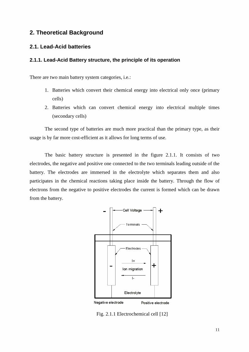
The basic battery structure is presented in the figure 2.1.1. It consists of two

electrodes, the negative and positive one connected to the two terminals leading outside of the

battery. The electrodes are immersed in the electrolyte which separates them and also

participates in the chemical reactions taking place inside the battery. Through the flow of

electrons from the negative to positive electrodes the current is formed which can be drawn

from the battery.

Fig. 2.1.1 Electrochemical cell [12]

12

The basic battery structure is suited for both types of batteries. A battery is

characterized by the chemical reaction taking place inside of it, the cell reaction. In order to

properly explain the battery operation a closer look must be taken into the cell reaction of the

battery [12]. Fully charged battery contains only high energy chemical compounds, which are

converted into lower energy compounds during the process of discharging. Similarly, when

the battery is charged the reaction is reversed, requiring sufficient amount of energy to be

supplied to the cell. In the batteries, the cell reaction is divided into two separate electrode

reactions by design in order to ensure that the released energy takes form of electrical energy

instead of heat. The current is created by the flow of electrons between two electrodes. The

cell reaction for the battery is as follows[12]:

(1)

Where:

(2)

(3)

S(N) – negative substance

S(P) – positive substance

– oxidized

red – reduced

During the process of discharging the battery, according to the presented chemical

reactions, the substance in the negative electrode is oxidized by the oxidizing substance. It is

located in the positive electrode and is reduced as a result of the process. The energy that can

be drawn from the cell is represented by the difference of chemically bonded energy between

the starting and the final composition of the cell reaction (1). However, it must be noted that

part of the energy is lost as a heat in the process.

2.1.2. Electric model of the battery

In order to give better understanding of the operation of batteries, electrical network of

the battery is introduced by using typical electrical components. This process is of great help

for an electric engineer to analyze the behavior of the battery, as it’s based on his primary

13

knowledge. Battery is an electric bipole, so it could be represented simply by electromotive

force and an internal impedance, if it were linear. However, the battery is nonlinear, meaning

that both the electromotive force and impedance are functions of the battery state of charge.

Electrical model which takes into account the nonlinearity of the battery as well as the fact

that its charge efficiency will not be perfect is presented in figure 2.1.2. :

Fig. 2.1.2 Electric model of a general battery considering the parasitic reaction [3]

Firstly, it should be noted that the elements Z and E are function of the battery state of

charge (SOC) and the electrolyte temperature (Θ). It can be observed that only some part (Im)

of the total current (I) take part in the main reaction. The p branch represents the parasitic

reactions present in the battery, energy in the p branch is converted into other forms of

energy. In the case of the lead-acid batteries the energy is absorbed through the water

dissociation reaction, which is the separation of oxygen and hydrogen. Dissipation of the

thermal power in the impedances Zm and Zpis the source of heating of the battery.

With the addition of a priori knowledge, the conditions for inactiveness of the parasitic

branch, the model presented in figure 2.1.2 can be simplified, representing a specific type of

battery. The electrical model for the lead-acid battery is presented in the figure 2.1.3. In the

case of lead-acid batteries, their charge efficiency is very close to unity while the voltage is

below a threshold level on the battery [3]. The model is divided into two branches, the

parasitic and the main reaction branch represented by p and m indexes respectively.

The identification of the main branch can be done by observation of the battery step

responses, the input can be set as step current from the constant value of I to 0, the observed

output is the battery’s voltage. With the assumption that the parasitic branch is inactive,

meaning it draws no current, the identification will be simpler. The measurement of the

battery step responses is done at different SOC and electrolyte temperature values. The

14

process of identification in this case is very complex and highly dependent on the number of

R-C blocks. Moreover, the model parameters change at different paces depending on the

environment they are used in.

The parasitic branch is less complex. Experimental work has proven that [3] internal

impedance Zp could be modeled as a simple resistor. However, the model cannot be designed

as linear since there is a nonlinearity in the relation of the current Ip with the voltage at

parasitic branch terminals VPN.

Figure 2.1.3 The electric network model for lead-acid batteries [3]

In the figure 2.1.3 the resistor R2 is a function of the state of charge of the battery

(SOC). The presented model requires a choice of reference current I*. The choice of reference

current as well as all of the necessary equations are shown in detail in [3]. The capacitance is

dependent on the electrolyte freezing temperature and empirical coefficients which are

constant for a given battery and chosen reference current.

2.1.3. Lead-Acid battery types

The lead-acid batteries can be subdivided into the three categories, in accordance to

technology used in the battery construction, i.e:

Vented/wet cell (flooded) batteries

Absorbed Glass Mat (AGM) batteries

Gel cell batteries

15

Vented/wet cell (flooded) batteries

Flooded batteries are the most commonly used lead-acid batteries nowadays. Due to

their relatively low prices (compared to the gel and AGM batteries), many size options and

versatility, they have found their application in a variety of industrial branches. The term

"flooded" is used to indicate the excess of electrolyte fluid, in which the plates are completely

submerged [17]. The use of wet cell batteries has many advantages. Not only the flooded

lead-acid batteries can be easily maintained by adding distilled water, but also their operations

are much more stable in high temperatures (>32° C) compared to the other types. Moreover

they are widely available and have a long history of use, which in some way proves their high

reliability and usefulness. On the other hand these kind of batteries may be used only in

upright position. They produce oxygen and hydrogen when charging, and then require

constant ventilation. It may produce hazardous acid spray if it gets drastically overcharged

and has a higher discharge rate than the other types of Lead-Acid Batteries. This type of the

battery will be used during the project presented in this paper.

AGM (Absorbed Glass Mat) batteries

AGM is one of the types of VLRA (valve regulated lead acid battery). In this system

fiber separators are introduced to prevent the leakage of acid. It is achieved through

absorption of the liquid electrolyte [12], while allowing a number of the pores to be empty.

Those unfilled pores are channels, through which the oxygen can migrate from the positive to

negative plates. The glass mat absorption property is crucial in the process as it allows high

compression of the gel and a narrow contact may be maintained between the plates and the

separator [17]. The separator should not be saturated with liquid, in order to keep the pores

free for the oxygen migration. AGM batteries have numerous advantages, i.e. they are less

expensive than Gel batteries, have slowest self-discharge from all of the types, best

shock/vibration resistance and much wider temperature range than Gel or Flooded batteries

[17]. However, the initial capacity is slightly lower than the capacity of vented batteries

(around 80% of the comparable flooded battery [12]).

16

Gel Cell batteries

Although the gel cell battery bases on oxygen recombination, the method to achieve it

slightly differs. This kind of batteries is filled with a thixotropic gel of silica mixed with

sulphuric acid [17]. All of the space in the battery is filled with it, forming a solid matrix. In

the beginning of a battery life time it behaves exactly like the flooded type as all of the

separator's pores are filled and there are no oxygen channels at all. With time the gel dries out,

shrinks and forms a numerous cracks, creating the oxygen channels, which allows the oxygen

to migrate to negative plate and therefore be recombined. The gel batteries perform better than

AGM batteries in two cases, in low power applications and when the regular deep discharge is

required [17]. There are several drawbacks of the gel batteries as well, e.g. they are more

expensive than other types, have much higher self-discharge rate than AGM batteries and are

less operational at low temperatures (<40 degrees F).

2.1.4. Lead-acid batteries applications

Lead-acid batteries are a significant part in everyone's everyday life. They serve as a

starter battery for vehicles - cars, buses, electric forklifts, wheelchairs, public transportation

and boats. They are the main emergency power supply for different electrical systems,

ensuring that the most important devices are operational and no data is lost during the

blackout situations. The lead-acid batteries are crucial for telecommunication companies as

they enable back-up supply during the cataclysms and power outages [18]. The three main

types of lead-acid batteries (i.e. flooded, AGM and gel) have found their specific applications,

e.g. the valve-regulated batteries are preferred in the systems that require high deep discharge

ability and the maintenance cannot be undertaken (maintenance-free VRLA batteries).

Furthermore the VLRA batteries are operational in horizontal position and do not require

ventilation, what may save a lot of space, which is a crucial feature in battery rooms.

2.2. Other popular battery types and their applications

Apart from the lead-acid batteries there are four most commonly used battery types:

lithium-ion, lithium-air, nickel-cadmium and silver-oxide batteries, which applications will be

described briefly as this project is focused on lead-acid batteries.

17

Lithium-ion (Li-Ion) battery is more stable version of its predecessor - lithium metal

battery. Li-ion battery finds its application both in easily recharged devices, such as cell

phones and in systems, in which recharging is difficult or impossible, e.g. cardiac

peacemakers. It can handle large number of recharges, without losing much capacity, making

it a perfect battery for portable electronic devices. Li-ion batteries are useful in the medical

application, i.e. as a battery for implantable electronic devices - pacemakers, defibrillators,

neurostimulators etc. as they are small, reliable and able to last for years [12].

Lithium-air battery - another lithium-based battery, introduced in early 1990s, is still

in the stage of development. This type of battery is expected to replace the lithium-ion

batteries, as its energy density is potentially five to fifteen times larger [1]. Currently most of

the li-air battery applications concern the automotive industry as weight is a primary concern

there.

Nickel-cadmium (Ni-Cd) battery is a standard for second type of batteries. Being very

durable and scalable they are often used in a variety of industrial machines, such as a portable

machinery or heavy duty tools, when other sources of power are not available. Due to their

ability to work in a harsh environmental conditions, they make perfect batteries for the

machines vulnerable to dust and dirt, such as portable drills, portable communication tools,

like two way radios (walkie-talkie type) and other field equipment [12].

Silver-Oxide batteries are known for their long operating life. The small silver-oxide

batteries are relatively cheap and have many advantages over other types of cells. Their

operating voltage is higher than mercury batteries. Silver-Oxide batteries are capable of

providing nearly instant high power even after prolonged use in high temperature

environment [8].

2.3. Battery variables

There are a number of variables which need to be known in order to build a proper

model of a battery. The list of the most important ones will be presented below:

Voltage

There are two methods of deriving the voltage of a battery, depending on the

reversibility of the system. Cell voltage can easily be derived from the thermodynamic data, if

the system is reversible [12].

18

The equation representing the reaction from which the equilibrium voltage can be derived is

as follows :

Where:

= free enthalpy of reaction, the maximum amount of chemical energy that can be

converted into electrical energy and vice versa

n = number of exchanged electronic charges

F = Faraday constant

It is necessary to distinguish the difference between the open circuit voltage (OCV)

and the closed circuit voltage (CCV). Most of the systems are not reversible and thus require

the measurement of OCV, which can also be used as a mean to determine the SOC of the

battery. Deriving closed circuit voltage (CCV) is much harder, due to its dependence on the

current, SOC and the history of the cell [12].

Capacity

Capacity of the battery is defined as a number of electrical charges in Ah units which

can be drawn from the battery. This parameter decreases steadily with the aging of the battery.

Proper estimation of the change of battery’s parameters is imperative for long term use of the

battery. Precise estimation of the capacity is dependent on many variables, most significantly:

Design of the battery

Discharge current

Temperature

Moreover, the important variable with regard to both capacity and the state of health

(SOH) is the depth of discharge (DOD). In case of lead-acid batteries, deep discharges below

the maximum value of DOD can rapidly decrease its service life [12].

Internal resistance

Internal resistance is used in order to measure the capability of the battery to handle a

load, as well as to determine its power output. The general rule concerning DC resistance is

19

that it must be significantly lower than that of the load. However, it must be noted that the

term does not represent simple ohmic resistance, as it depends on the operational conditions

as well as the SOC of the battery. The internal resistance can be calculated using the direct-

current method:

Direct-current method compares the voltage at two different loads. The current i1 acts

as the first load, resulting in appearance of voltage U1. Afterwards, the current is increased to

the value of i2 leading to decrease in voltage up to the value of U2.

Deriving the AC internal resistance of battery is a complex procedure, as the AC

characteristics of the battery cannot be obtained directly, but through approximation of an

equivalent circuit. This issue will not be explained in the paper.

Self-discharge

Self-discharge parameter represents the losses of charge in the electrodes while the

battery is in open circuit. There are many reasons for the self-discharge, few of which are

listed below [12]:

Gradual reduction of the oxidation state in the positive electrode

Mixed potentials in the secondary reactions

Oxidizable or reducible substances in the electrolyte

There are also several processes which are misinterpreted as self-discharge, ex. increase

in the internal resistance that happens after prolonged storage of primary cells, and causes a

reduction in delivered capacity.

2.4. Lead-Acid battery aging process

Due to the nature of lead-acid batteries operation, which is based on conversion from

the chemical energy into electrical one, several major aging processes occur [11]:

20

Anodic corrosion

Positive mass degradation

Irreversible formation of lead sulfate in the active mass

Short circuits

Loss of water

Important term when considering the aging process of a battery is its state of health

(SOH). It is used as indicator of the performance of the battery both in the state of charge and

discharge, it may also contain information concerning the degradation of the battery. In order

to design a method to predict the lifetime of the battery major ageing processes must be taken

into account as well as the interaction between them [13]. Developing proper tests to analyze

the complex interactions and linking them to the lifetime expectancy has proven to be great

challenge. It has been proven that differentiating the effects of single ageing process can be

possible only up to a certain level [13].

2.5. State of charge monitoring methods for lead acid batteries

As mentioned in the last chapter, lead acid batteries are used in numerous applications,

which require high reliability, robustness and predictability. The reliable state of charge

estimation strategy is a necessity in such uses as hybrid vehicles, electric vehicles and

telecommunications power supplies, therefore several ways of SOC estimation are widely

known in the industry. Accurate method of the SOC estimation may prevent the battery from

getting deeply discharged or frequently overcharged, both of which greatly reduce the battery

remaining life. Before the methods will be presented, it is important to state the SOC

estimation accuracy, which is demanded for the different battery applications.

In Hybrid Electric Vehicles (HEV) the battery acts as a starter for the motor so any

imprecise SOC readings with an error over 5% can seriously affect the engine's fuel efficiency

and the motor operations. For the following reason in HEV applications the SOC estimation

must be as precise as possible with an error's value never exceeding the 5% of the capacity

measurement [16].

However, in Electric Vehicles (EV) the battery SOC determines the distance the

vehicle is able to cover. The battery SOC in electric vehicles resembles the fuel tank from

traditional vehicles, which are notoriously imprecise (usually about 5% measurement error) so

21

the borderline of 5%-7% errors in the EV applications could possibly be acceptable. During

the process of designing the SOC estimation method for EV it is important not to mistake the

state of charge with the capacity of a battery. Those two are usually mistaken because of their

equality in the beginning of the battery use, however they begins to differ with the decrease in

the battery state of health. SOC estimation is highly dependent on the battery aging process

and after a certain number of charging/discharging cycles 20% or bigger error may occur [16].

For that reason state of charge of a battery should estimate the energy content and the power

capability of a battery.

2.5.1. Open circuit voltage method

The OCV method uses the voltage of a battery cell as an indicator of a current battery

SOC. The SOC of a battery as a semi-linear function of the open circuit voltage as presented

in the figure 2.5.1. Although the open circuit voltage method is known as an accurate

indicator of the SOC, this method cannot be regarded as a real-time monitoring strategy as the

voltage readings take much time to stabilize. The OCV stabilization example is shown in the

figure 2.5.2. Results of this method can vary depending on the measurement conditions, ex.

actual voltage level, temperature, discharge rate and the age of the cell [6].

Fig. 2.5.1 The open circuit voltage to residual capacity relation of lead acid battery

experiment.

22

Fig. 2.5.2. The stabilization of the OCV after being disconnected from the load.

2.5.2. Specific Gravity (SG) method

Measurement of the specific gravity of the electrolyte is equivalent to testing the

concentration of acid (sulphuric acid) in the electrolyte. During the battery discharging

process the active material is consumed and its concentration decreases. The Specific gravity

(SG) test can be performed using a traditional hydrometer, which is time consuming process

and cannot be performed in a real time so another method is preferable, i.e. using a modern

digital sensor, placed inside the cell, which updates the state of electrolyte continuously [16].

This method, however is only briefly described in the literature and the specific gravity/

electrolyte density proportions may vary depending on the producer of the battery [16, 19].

2.5.3. Coulomb counting method

Current integration method (also called a direct method) is a simple process of

summing of capacity taken out from the battery. The current SOC of a battery is simply a

maximum charge minus the current, multiplied with time for which it was flowing.

23

Theoretically, this method is an obvious and simple choice to implement, however, practically

it has many disadvantages. The current flow is not constant, but changes with the battery

operations, the longer the method is used the bigger the error gets due to the presence of an

integral. Furthermore this method relies on a discharging process, thus without the knowledge

of a discharge data (i.e. time, discharge current) the user is simply unable to estimate the

current SOC.

2.5.4. Impedance measurement method

Impedance is another variable that characterizes a battery, which changes with

charging/discharging processes. The change in active chemicals in the cell affects the change

of its impedance. The measurement of a battery internal impedance is also a way to estimate

the SOC, however, it is not a common strategy due to its complexity and temperature

dependence [16].

2.6. Battery modeling techniques

In order to fully understand the operation of a battery different approaches must be taken,

as the problems cover many fields of science. In order to help solve these problems several

model types were created, amongst which the most common are:

Electrochemical models

Physical models

Equivalent circuit models

Each of the presented models gives different perspective into explanation of the behavior

of the battery from their respective field of science. Such separation was created so that

knowledge from just one of the areas is sufficient to understand the processes taking place

inside the battery.

Electrochemical models focus mostly on the chemical reactions taking place inside the

battery. This type of battery model finds its use in construction and design of the battery.

However, many parameters of the battery are very hard to describe using these models, such

as internal resistance, which makes them not feasible to represent the dynamically changing

key variables describing the battery behavior. However, the dynamic properties of battery can

24

be obtained by analyzing the consistency of the substances taking part in the electrochemical

reaction caused by connection of electrodes to external circuit.

Physical models represent the operation of the battery through mathematical and physical

equations. Two main methods used for creation of those models can be distinguished, which

are the finite number and the computational fluid dynamics technology. These methods allow

deep understanding of the fluid and mass flow as well as heat transfer which are important for

the operation of the battery. However, high computational power is required due to many

complex calculations. Moreover, the process requires a lot of time which deems the model

unusable for the purposes of the project presented in this paper.

Equivalent circuit models represent the electrochemical parameters and the behavior of

the system through the creation of simplified, equivalent circuit consisting of electrical

elements. The simplicity of these models can vary greatly depending on the required level of

precision. These models are easily adjustable to specific requirements while maintaining the

lowest possible level of complexity. Equivalent circuit model was chosen for the project, due

to its ability to follow the dynamically changing variables with reasonable computational

power requirements. Example model of this model type, as well as its explanation was

presented in the chapter 2.1.2, “Electric model of the battery”.

2.7. Electric equivalent circuit models

2.7.1. Simple battery model

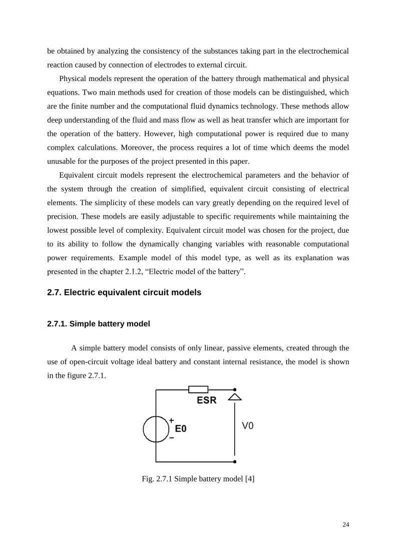
A simple battery model consists of only linear, passive elements, created through the

use of open-circuit voltage ideal battery and constant internal resistance, the model is shown

in the figure 2.7.1.

Fig. 2.7.1 Simple battery model [4]

25

Where :

ESR – internal series resistance

Vo – terminal voltage of the battery

Eo – open circuit voltage

The model it is mostly used in systems where the battery doesn’t have too high of an

influence on the circuit. It is incapable of describing the battery behavior due to the lack of the

relation of internal resistance in different states of charge (SOC).

2.7.2. Advanced simple battery model

An advanced simple battery model is an improved version of the simple battery model

through the addition of the dependence of internal resistance on the SOC [4]. The

configuration of this model is the same as the simple battery model, presented in figure 2.7.1.

The relation between the internal resistance and the SOC is represented by equation:

Where:

R0 - resistance of the fully charged battery

SOC – state of charge of battery

k – capacity coefficient

2.7.3. Thevenin battery model

Thevenin battery model is another commonly used model which was designed to

account for transient behavior of the battery. The model is shown in the figure 2.7.2. The R0

parameter represents the resistance between the contact plates and electrolyte while the C0

relates to the capacitance between the parallel plates [4]. The big disadvantage of the thevenin

model is the assumption of constancy of all the elements, as they all depend on the SoC and

other battery characteristics.

26

Fig. 2.7.2 Thevenin battery model [4]

Where:

E0 – ideal battery voltage

R – internal resistance

C0 – capacitance

R0 – resistance between the contact plates and electrolyte

2.7.4. Modified Thevenin Model

The improvement to the basic Thevenin Battery Model has been done by Farell [2].

The improved model is presented in the figure 2.7.3.

Fig. 2.7.3 Modified Thevenin equivalent circuit model [7].

The charging/discharging equations are given by

27

Where:

Rd and Rc are two kinds of internal resistances of a battery. The diodes are used to

imply that during the charging and discharging processes only one of the internal resistors

will be taken into account, depending on the current flow's direction. The polarization

capacitance is represented by the capacitor C. The improvements to the model enable it to

account for dynamic changes taking place inside of the battery.

2.7.5. Third-Order Battery Model

A Third-Order Battery Model is presented in the figure 2.7.4.

Fig. 2.7.4 A Third-Order Battery Model [7]

The model is divided into the main, and the parasitic branch. It consists of two R-C

blocks, ideal source of energy (Em) and two resistors R2 and Rg. This model is particularly

interesting due to its relation to the SOC calculation and the internal electrolyte temperature.

Some of its computational elements are the functions of state of charge and the temperature,

which is an unquestionable advantage comparing to the previously described models. The

variables are the currents I1 and I2, the state of charge Qeand the electrolyte temperature [7]

The dynamic equations for this model are as following:

[

]

28

Where :

(

(

))

And:

Em0, Gp0,Vp0,Ap are constants for a particular battery

= thermal resistance between the battery and its environment

= temperature of the environment

2.7.6. Simplified equivalent circuit model

A simple battery model structure was introduced in [10] and is introduced in the figure

2.7.5. An author of the paper approached the problem with the simplicity-oriented attitude.

Fig. 2.7.5 The equivalent circuit model for a simplified method.

Where the relations between the variables are as following:

(

)

29

(

(

))

And :

Em0 = open circuit voltage at full charge

KE = constant

= electrolyte temperature

R00 = value of R0 at SOC = 1

= main branch time parameter in seconds

Im = main branch current

I* = nominal battery current

A0,KE, R10, R20, A21,A22= constant

Introduced structure does not take the lead-acid battery’s internal chemical processes

into account, however, it temporarily approximates the processes which may be observed

during the battery work. It consists of two circuits: the main branch approximating the battery

dynamics in typical circumstances, and a parasitic branch, which imitates the battery behavior

at the end of its charging. Every element of the circuit is based on non-linear mathematical

representation and is a function of SOC, DOC (depth of charge) or temperature. The

equations' variables are dependent on the determined constants. The electrolyte temperature,

voltages, currents and stored charge are regarded to as states.

3. Algorithm design and implementation

In the beginning of this chapter the problem will be presented and analyzed. In the

next step, the requirements for the algorithm will be introduced, leading to a theoretical

design of a suitable and implementable algorithm, which fulfills the specifications. In order to

have a comparison, an alternative method will be chosen, presented and described in details. It

will later be used in the testing phase to provide alternative SOC estimation tool and a method

to be compared with. The final part of the chapter will include the detailed description of a

laboratory setup, which was used for both implementation and testing. As a chapter's

conclusion, the practical, step by step instruction covering the implementation of a designed

SOC estimation algorithm will be introduced.

30

3.1. Project requirements

To enlist the requirements the problem must be first described and analyzed. With the

cooperation of a Swedish company - Micropower (www.micropower.se) - Research and

Development department the problem of an electric forklift's Lead-Acid Batteries SOC and

SOH will be introduced.

First of all, Electric Vehicle acts as a highly variable load so the current drawn from a

battery is not constant during the discharge phase. The designed SOC and SOH estimation

software should operate in real-time, providing the forklift's operator with the crucial

information - the SOC and SOH of the battery at any given moment.

The method will be designed and tested in Mathworks MatLab® environment, the

project group will try to ensure that it is translatable and implementable in C programming

language. Such solution would make it possible to be added as a feature for the operator's

onboard Human - Machine Interface.

Typical voltage and current curves during the battery discharge are presented in the

figure 3.1.1. Presented data was gathered during the real forklift's operations in Micropower.

The sampling interval is 4 minutes, which is too long for a data to be called precise and thus

useful in the tests as not accounting for changes during those periods may increase the error in

SOC estimation. However, it clearly shows the changes in load during the discharge phase of

a forklift's battery.

Fig. 3.1.1 Voltage and current discharge curves during forklift's operation with 24V battery.

31

There is no apparent pattern in current drawn during the battery discharge, it depends

on the load that the forklift provides during its operation. The current values vary between 0A

and 32A throughout the pictured 142 samples (9 hours of operations, regular work day).

There are moments in which the battery is put on hold, when the current drawn is lowered to

0A and the voltage slowly stabilizes to finally become the Open Circuit Voltage. In those

moments the OCV/SOC linear characteristic can be used to provide a reliable SOC

estimation.

Terminal Voltage (a measured voltage, when a battery is under load for a certain time,

also called closed circuit voltage (CCV)) is highly dependent on a load. Furthermore,

TV/SOC characteristic is nonlinear and depends on the battery type, nominal capacity,

temperature and load, making it less useful than the OCV/SOC characteristic. For this

dynamical part of voltage characteristic the Coulomb Counting method or its improved

variations can be successfully applied.

The fully charged 24V battery’s Terminal Voltage is around 24,8V and the cut-off TV

is around 24,1V, which is approximated to 20% SOC point. This specific value is optimal to

stop discharging the battery in order to ensure that deep discharge does not occur. Avoiding

the deep discharge is highly desired by the customer as it greatly prolongs the battery’s life.

Micropower's Battery Monitoring Unit (BMU) will be used as a measurement tool in

the project. It provides the user with the real-time voltage, current and internal temperature

measurements and transfers the data via Wi-Fi, communicating with the company's software

installed on the PC.

Although the project focuses on the discharging process (estimating the battery SOC

while it is under discharge) data gathered during the charging process may also be of use. The

main charging peak consists of around 45 first samples, the rest of the process are the

"maintenance" current spikes. During 3 hours the battery is loaded with certain pattern. The

usefulness of the charging curve lies within the information on how much Ampere-hours have

been transferred to the battery and what value the OCV have after the charging is finished.

Those two information will be used in the algorithm to improve its performance. Several

equivalent circuit models use the current measurement to estimate the battery internal

temperature and voltage. There is no need to estimate values, which can be successfully

measured with the BMU so the focus in this project will be put on using all the available

measurements to estimate SOC and SOH. The charging phase of the very same battery is

presented in the figure 3.1.2.

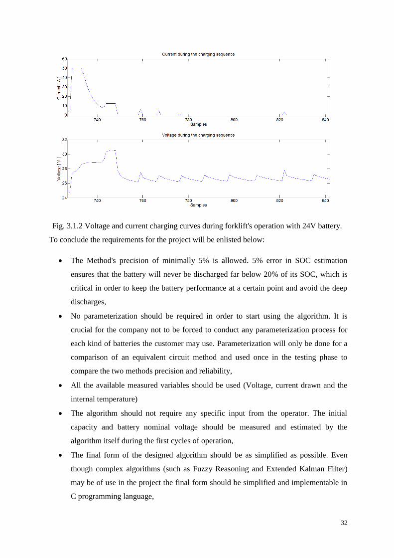
32

Fig. 3.1.2 Voltage and current charging curves during forklift's operation with 24V battery.

To conclude the requirements for the project will be enlisted below:

The Method's precision of minimally 5% is allowed. 5% error in SOC estimation

ensures that the battery will never be discharged far below 20% of its SOC, which is

critical in order to keep the battery performance at a certain point and avoid the deep

discharges,

No parameterization should be required in order to start using the algorithm. It is

crucial for the company not to be forced to conduct any parameterization process for

each kind of batteries the customer may use. Parameterization will only be done for a

comparison of an equivalent circuit method and used once in the testing phase to

compare the two methods precision and reliability,

All the available measured variables should be used (Voltage, current drawn and the

internal temperature)

The algorithm should not require any specific input from the operator. The initial

capacity and battery nominal voltage should be measured and estimated by the

algorithm itself during the first cycles of operation,

The final form of the designed algorithm should be as simplified as possible. Even

though complex algorithms (such as Fuzzy Reasoning and Extended Kalman Filter)

may be of use in the project the final form should be simplified and implementable in

C programming language,

33

All the measurements will be done by the Micropower BMU and then transferred and

processed in MatLab environment in order to conduct the tests.

3.2. Reference method

It was decided that the designed method will be compared with another one from the

literature. The OCV estimation method, based on the article “Estimating the State of Charge

of a Battery” by John Chiasson and Baskar Vairamohan, published in “Transactions on

Control Systems Technology” was chosen as a reference. A Modified Thevenin circuit was

used for modeling the battery’s behavior as it accounts for energy losses in all forms as well

as the transient behavior of the internal current of the battery. In this section a more in-depth

theoretical description of the model will be given as well as the algorithm for the method.

Practical implementation of the model in MatLab environment will be presented in the section

2.5 “Implementation”.

Fig. 3.2.1 Modified Thevenin equivalent circuit model [7].

The description of basic electric elements present in the model was given in section

2.7.4, electric equivalent circuit is presented in figure. 3.2.1. However, it should also be noted

that the polarization capacitance C is not purely electrical capacitance as portion of it is due to

chemical diffusion within the battery. Energy loss in the battery in all forms is modeled

through the use of three resistances: Rc, Rd, Rb which stand for charge, discharge and terminal

resistance respectively. The terminal current of the battery Ib have positive values during

discharge process [5].

34

The purpose of the method is to estimate the battery’s SOC based on OCV assuming

that only terminal voltage and current can be directly measured. It also should be stated that

parameters: Rc, Rd, Rb, C, Vp are neither known a priori nor can be measured. The algorithm

of the method will be presented in several steps. In this paper, a short summary of the method

will be presented. It is strongly based on [5] and more detailed information can be found

there.

1). Define the state variables:

(1)

Where:

Vp – capacitance voltage

Rd – discharge resistance

Rc – charge resistance

Rb – terminal resistance

C – polarization capacitance

2). Create nonlinear time-varying state-space model:

Where :

is unknown,

The open circuit voltage can be derived from (1).

35

3). Create the system in the form of:

Where : z1 = x1 , z2 = x3, z3 = x4, z4 = x5.

The reason for excluding the state x2 is presented in the step 6. The exact value of the

state is presented in equation (1).

4). Definition in order to Check the observability of the system

Firstly, the system is to be rewritten in a more compact form:

(2)

) (3)

(4)

Where:

Secondly, transition matrix of the system is defined as:

(5)

(6)

Where:

(7)

36

(8)

The system is observable on [t0,tf] if and only if the Gramian matrix M is invertible [5].

∫

(9)

If the matrix M is invertible, the initial values of z(t0) can be found through the integration of

a multiplication of y(t) by :

∫

(10)

∫

(11)

5). Find conditions for non-singularity of the Gramian

In order to calculate the the matrix M must be non-singular, the process of

finding the conditions for such feature is as follows:

By solving the equation (7) for :

(12)

(13)

(14)

(15)

With:

, i = 2,3,4 and j = 1,2,3,4 (16)

Results in :

Where:

,

, ∫

37

Assume that over any short time interval, the battery current waveform can be fit to quadratic

equation:

(17)

If we combine (17) with the definition of we get:

6). Calculation of the OCV

As

, however it was proven in [5] that the VOC is not asymptotically

dependent of x20. The given solution to the problem was to use arbitrary value of in

equation (17)

- (

- ∫

) (18)

3.3. Designed method

For the time being, the Battery Monitoring Unit (BMU) uses well-established coulomb

counting method in order to calculate the remaining State of Charge of the battery during

discharge. As the currently implemented algorithm produces error, which is unacceptable in

forklift's operations, it is reasonable to improve it. The designed algorithm is based on the

very same coulomb counting, but also the measurements, which are currently unused, such as

terminal voltage and the battery internal temperature.

The algorithm was designed during laboratory discharge tests and bases mostly on

observations and empirical knowledge. In [9] the authors used similar approach, creating a

method that corrects the SOC readings depending on the discharge current profiles. The

method presented in the paper is called "Enhanced Coulomb Counting" and works well with

38

the discharges under constant load. As mentioned before, the forklift's operations include the

nonlinearly-changing load, making the method from [9] not valid for our application.

Although the coulomb counting method is widely used, it generates relatively high

error and is too dependent on the ampere-meter readings, and thus is not reliable as a stand-

alone method. On the other hand, there is an almost linear OCV/SOC relation, which gives

solid results with very low error values. However, in order to obtain open circuit voltage

readings, the battery must be disconnected from the load for a certain amount of time, what

hardly ever happens in forklifts daily operations. The algorithm can be regarded to as

"Improved Coulomb Counting" as it uses the coulomb counting as a primary method, but

corrects it with the correction factor. Its values depend on the error between the SOC

calculated with Ah counting and SOC derived from OCV/SOC diagram.

Typical forklift’s daily operations consist of around 9 hours under variable load with

numerous breaks, each being too short to estimate the battery's OCV with a sufficient

precision. Those breaks enable the algorithm to estimate the OCV from the "Semi-OCV"

values that occur after a certain amount of time without flow of the current. Typical battery

voltage behavior after disconnection from the load is presented in the figure 3.3.1.

Fig. 3.3.1 Battery Voltage after being disconnected from load.

39

The sample time is set to 2s. The graph presented in figure 3.3.1 covers around 1800

samples, which is 1 hour of data collection. The red dotted points, namely T0, T1, T2, T3 are

pre-counted points referring to:

T0 - first sample when the current has 0 value,

T1 - the moment, when the voltage starts being constant for 30 samples (60 seconds),

T2 - the moment, when the voltage starts being constant for 150 samples (5 minutes),

T3 - the moment when the voltage starts being constant for 2700 samples (90

minutes).

Those 4 points must be pre-counted, i.e. the algorithm needs a long (preferably more than

2 hours) rest after the first discharge. It has been proven that the real Open Circuit Voltage

value might be measured after 1.5 hours with the battery disconnected from the load, and the

changes dynamics had not changed over numerous discharge tests (Figures 3.3.1 - 3.3.6). T1,

T2 and T3 had been counted from T0. Those numbers are intervals between the moment

battery is put on "hold" and the voltage is constant for a certain amount of time.

As pictured in the figure 3.3.1, the voltage does not change significantly between the

T1, T2 and T3 points. The voltage in T3 moment is 0.02V higher than in T2 point and 0.04V

higher than in T1 point. This relationship has been proven correct, no matter what the

discharging current values were before the battery was put on hold and how long the

discharge lasted. This similarity is used in the algorithm, ex. even if the rest time of the

battery is much shorter than required in order to measure the OCV, its value can be estimated

after reaching the T1 point (which in this case was 74 samples, around 2.5 minutes). The

relation between the voltages in T3, T2 and T1 points for the different discharge curves is

shown in the table 3.3.1.

# Figure Diff1 (T3-T1) (V) Diff2 (T3-T2) (V) OCV (V) Discharge (Ah) Discharge Current (A) Discharge time (s)

1 3.3.2 0.03 0.01 6.16 2.43 5 1753

2 3.3.3 0.04 0.02 6.00 81.18 11 26589

3 3.3.4 0.04 0.02 6.00 118.56 13 32840

4 3.3.5 0.04 0.02 6.03 13.68 14 3520

5 3.3.6 0.03 0.02 6.19 27.9 14 7178

Tab. 3.3.1. Comparison between the Diff1 and Diff2 throughout various discharge periods.

Although the general trend is followed the Diff1 and Diff2 voltages may differ

significantly between the tests – as Diff2 between #1 and #2 – 0.01 in value, but 100%

40

difference. That is why using Diff1 and Diff2 parameters will enable the algorithm to

estimate, not to define the precise SOC value in any given point of time.

Fig 3.3.2. Voltage after disconnecting battery from the load (5A, 30 minutes discharge).

Fig 3.3.3. Voltage after disconnecting battery from the load (11A, 8 hours discharge)

41

Fig 3.3.4. Voltage after disconnecting battery from the load (13A, 10 hours discharge).

Fig 3.3.5. Voltage after disconnecting battery from the load (14A, 1 hour discharge).

42

Fig 3.3.6. Voltage after disconnecting battery from the load (14A, 2 hours discharge).

The flowchart presenting the algorithm is presented in the figure 3.3.7.

Fig. 3.3.7 Flowchart presenting the logic of the algorithm's SOC correction.

The detailed instruction for implementing the algorithm is attached below:

1. During the first measured cycle of the battery, the operator has to be cautious as the

only source of SOC estimation is regular coulomb counting method. Thus it is

43

recommended to stop the discharge at least 10% before the SOC indicator reaches the

20% point. After the first discharge, battery should rest for at least 6 hours to enable

the algorithm to calculate the T1, T2 and T3 times.

2. After the T1, T2 and T3 delay times, as well as the voltage differences at those points

are saved in the memory, algorithm may proceed to the regular operation state.

3. During the regular algorithm's operations the SOC calculation is done based on the

basic coulomb counting. Ampere-hours drawn from the battery are added until the

moment load is disconnected. When battery is put on "hold" the correction factor has

to be counted.

4. If the discharge break is short, but long enough for the T1 period, OCV is estimated

based on the T1, by adding the previously counted difference (between T1 and T3

voltages) to the measured voltage. If the break continues and the T2 time passes the

algorithm updates by estimating the OCV in the T2 period the same way as with T1. If

the break lasts until the T3 time the measured voltage is taken as a real OCV,

improving the correction's precision.

5. The difference between counted Ampere-Hours sum divided by the SOH/Nominal

Voltage (giving the SOC estimate) and the previously estimated OCV translated to

SOC, using the SOC/OCV linear relation forms an error. It needs to be corrected

during the next hour of discharge in order for the SOC jumps to be avoided and make

the change look natural for the forklift operator. The other possible solution would be

to show the best known value to the operator, even though it will most form a “jump”

on SOC diagram.

6. The correction factor is counted using the error value and the average current

throughout the discharge:

7. For the next 1 hour, the current drawn is multiplied by this factor in order to reduce

the error caused during the last period of the discharge. Note that the correction is

done backwards and the factor is used delicately in order to avoid the jumps in the

current value and huge differences of the Ah-counting acceleration.

44

3.4. Laboratory setup

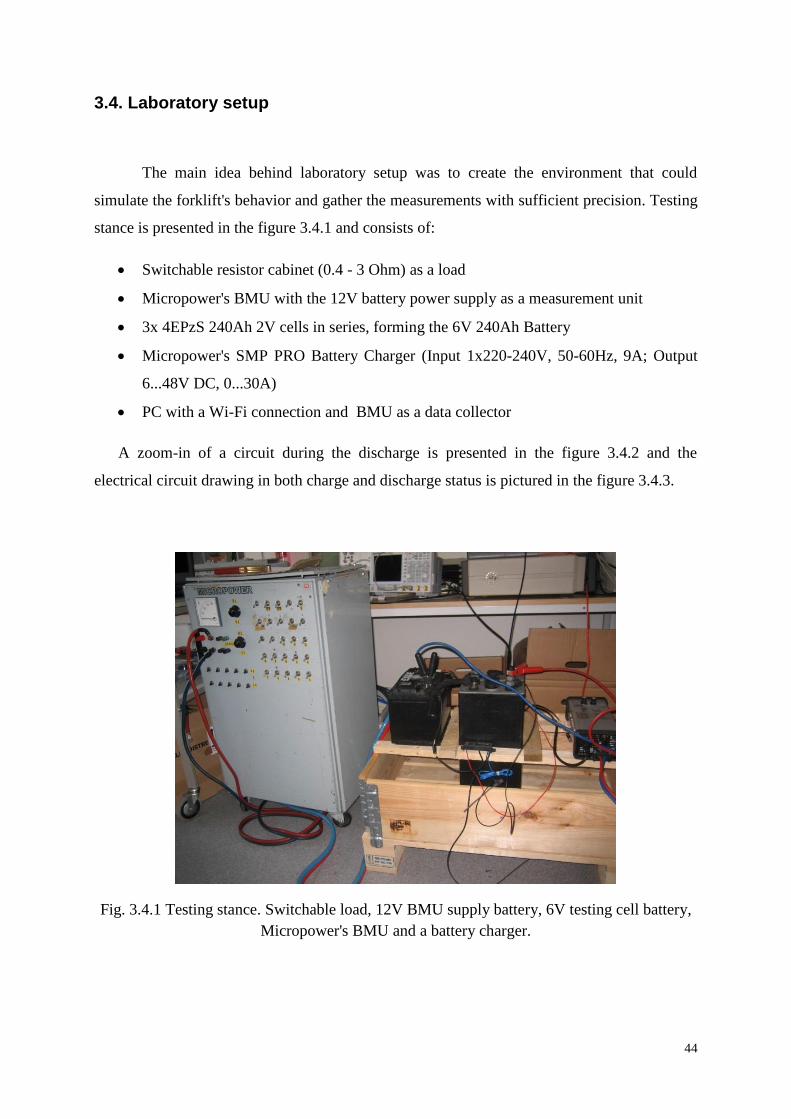
The main idea behind laboratory setup was to create the environment that could

simulate the forklift's behavior and gather the measurements with sufficient precision. Testing

stance is presented in the figure 3.4.1 and consists of:

Switchable resistor cabinet (0.4 - 3 Ohm) as a load

Micropower's BMU with the 12V battery power supply as a measurement unit

3x 4EPzS 240Ah 2V cells in series, forming the 6V 240Ah Battery

Micropower's SMP PRO Battery Charger (Input 1x220-240V, 50-60Hz, 9A; Output

6...48V DC, 0...30A)

PC with a Wi-Fi connection and BMU as a data collector

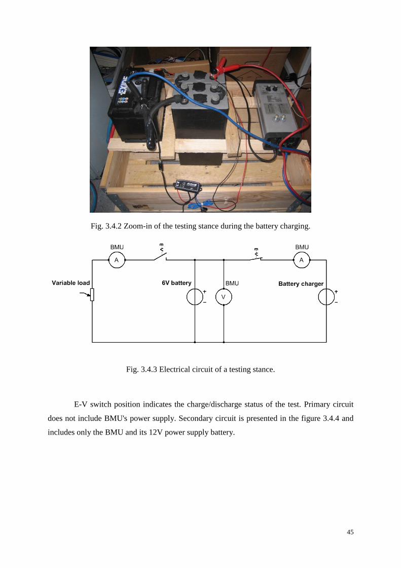
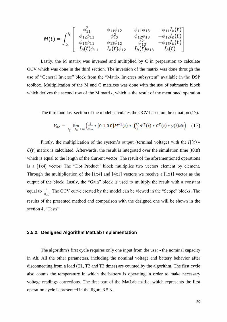
A zoom-in of a circuit during the discharge is presented in the figure 3.4.2 and the

electrical circuit drawing in both charge and discharge status is pictured in the figure 3.4.3.

Fig. 3.4.1 Testing stance. Switchable load, 12V BMU supply battery, 6V testing cell battery,

Micropower's BMU and a battery charger.

45

Fig. 3.4.2 Zoom-in of the testing stance during the battery charging.

Fig. 3.4.3 Electrical circuit of a testing stance.

E-V switch position indicates the charge/discharge status of the test. Primary circuit

does not include BMU's power supply. Secondary circuit is presented in the figure 3.4.4 and

includes only the BMU and its 12V power supply battery.

46

Fig. 3.4.4 BMU power supply circuit

Battery Monitoring Unit is capable of measuring both the Battery Voltage and

Current. Data collection is run with a sampling time of 2 seconds, which is enough to capture

even the slight changes of a current drain and the terminal voltage of the battery. The example

of a collected data, plotted in MatLab is presented in the figure 3.4.5

Fig. 3.4.5 Characteristic example collected with the testing stance.

47

3.5. Implementation

3.5.1. Reference Method MatLab Implementation

In this section, the practical implementation of the reference method will be presented.

The theoretical background of the method and the equations upon which it is based were

presented in section 3.3. Matlab R2012a environment was used in order to implement the

method. Firstly, the program written in the m-file will be presented in the figure 3.5.1:

Fig. 3.5.1 M-file code

48

The presented program enables reading the measured values of Voltage and Current as

a files saved by the BMU. The data gathered by the measurement unit is saved as csv file,

which is then read by Matlab using “fopen” command. The “textscan” command used in the

fifth line separates the gathered data into different columns. Measured values of the Voltage

and Current are assigned to the AvgCurrent and AvgVoltage arrays. Afterwards, two loops

are created in order to clear the data of the invalid values added by Matlab in the process of

reading the file. The x20 parameter is then initialized with an arbitrary value, which in this

case is equal to 3. Lastly, values of the Current and Voltage are saved as a “structure with

time” (structure consisting of a values vector and a time vector) for further use in the model.

The model created in the Simulink is presented in the figure 3.5.2.

Fig. 3.5.2 OCV estimation method model

In the first part of the model (highlighted with the blue border) the derivatives of are

computed according to the equations (11) – (13). For reading convenience the mentioned

equations are presented once again:

(11)

(12)

(13)

49

The value of the x20 parameter is constant and equal to 3. It is observed that only

is time variant as the derivative depends on the terminal current. In order for the model to

work it is necessary to run the script, prepared in the m-file presented in the figure 3.5.1 as the

measured values of voltage and current must be loaded into the workspace. It is also

imperative to set proper simulation time, equal to the length of time vectors of Ib and V

structures. In the section 3.2 “Reference method” it was stated that the intercepts of the Ib fit

to a quadratic equation (16)

(16)

should be used, however, practical implementation in Matlab environment allows for use of

the terminal voltage and current trajectories. The “Current” and “Voltage” blocks allow for

use of Ib and V variables from the workspace. One value from the vectors is used for each

simulation step in the Simulink. The “mux” block represented as black filled rectangle creates

a vector from the values of PHI11, PHI12, PHI13 and Ib(t) in the form:

Where:

Second section of the model calculates matrix M, its inverse and multiplication with

matrix C. Firstly, a transposed matrix of was created using the “transpose” block

from the DSP toolbox. Secondly, the aforementioned matrix was multiplied with its

transposed version which in result created a matrix in the form of:

Thirdly, the matrix was integrated on the (t0,tf) period, which is the simulation time of

the model. As a result the M matrix was created, which form is:

50

Lastly, the M matrix was inversed and multiplied by C in preparation to calculate

OCV which was done in the third section. The inversion of the matrix was done through the

use of “General Inverse” block from the “Matrix Inverses subsystem” available in the DSP

toolbox. Multiplication of the M and C matrixes was done with the use of submatrix block

which derives the second row of the M matrix, which is the result of the mentioned operation

The third and last section of the model calculates the OCV based on the equation (17).

(17)

Firstly, the multiplication of the system’s output (terminal voltage) with the

matrix is calculated. Afterwards, the result is integrated over the simulation time (t0,tf)

which is equal to the length of the Current vector. The result of the aforementioned operations

is a [1x4] vector. The “Dot Product” block multiplies two vectors element by element.

Through the multiplication of the [1x4] and [4x1] vectors we receive a [1x1] vector as the

output of the block. Lastly, the “Gain” block is used to multiply the result with a constant

equal to

. The OCV curve created by the model can be viewed in the “Scope” blocks. The

results of the presented method and comparison with the designed one will be shown in the

section 4, “Tests”.

3.5.2. Designed Algorithm MatLab Implementation

The algorithm's first cycle requires only one input from the user - the nominal capacity

in Ah. All the other parameters, including the nominal voltage and battery behavior after

disconnecting from a load (T1, T2 and T3 times) are counted by the algorithm. The first cycle

also counts the temperature in which the battery is operating in order to make necessary

voltage readings corrections. The first part of the MatLab m-file, which represents the first

operation cycle is presented in the figure 3.5.3.

51

Fig. 3.5.3 First cycle of the algorithm's operation (1/3)

Presented part of the code opens the pre-saved .csv (comma separated values) files,

saved by Micropower's BMU and transfers the Current, Voltage and Temperature data into

the MatLab workspace. The second part of the file is presented in the figure 3.5.4.

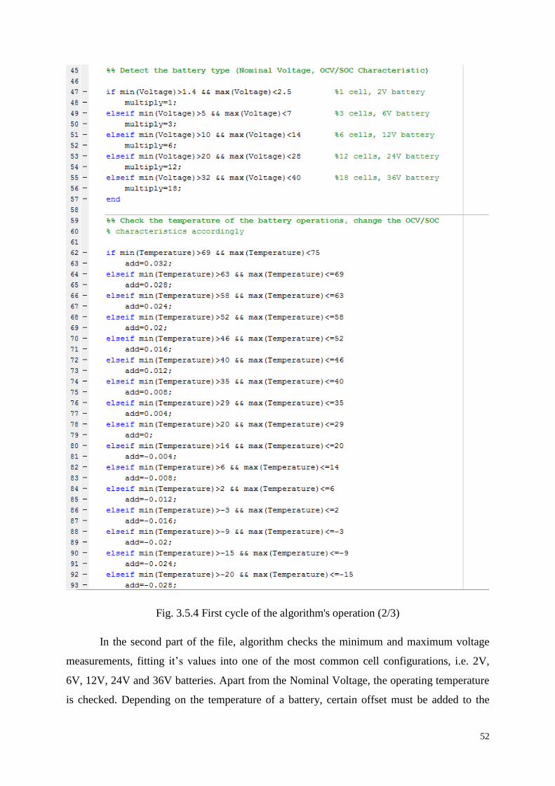
52


In the second part of the file, algorithm checks the minimum and maximum voltage

measurements, fitting it’s values into one of the most common cell configurations, i.e. 2V,

6V, 12V, 24V and 36V batteries. Apart from the Nominal Voltage, the operating temperature

is checked. Depending on the temperature of a battery, certain offset must be added to the

53

voltage readings. The temperature / voltage change relation for the Wet Cell Lead-Acid

batteries according to The Battery Council [14] is presented in the table 3.1. The operating

temperature of a battery is a critical factor and should always be included in the SOC

estimation, ex. Between 70°C and 10° C the open circuit voltage reading differs by 0,26,

translated to the OCV/SOC relationship not including the temperature difference produces

around 40% error in SOC estimation.

Temperature (°C) Voltage add (12V) Voltage add (2V)

71.1° 0,192 0,032

65.6° 0,168 0,028

60.0° 0,144 0,024

54.4° 0,12 0,02

48.9° 0,096 0,016

43.3° 0,072 0,012

37.8° 0,048 0,008

32.2° 0,024 0,004

26.7° 0 0

21.1° -0,024 -0,004

15.6° -0,048 -0,008

10° -0,072 -0,012

4.4° -0,096 -0,016

-1.1° -0,12 -0,02

-6.7° -0,144 -0,024

-12.2° -0,168 -0,028

-17.8° -0,192 -0,032

Tab. 3.1 Temperature/ voltage modification relationship for Flooded Lead-Acid batteries

Temperature of the cell varied between 20 and 22 °C throughout the whole testing

phase. However, the code above includes the possible temperature changes as a voltage

readings adjustment, ex. if the battery operated in 44 degrees the 0.012 V would be added per

cell to the readings, affecting the OCV/SOC graph. The third part of the file is presented in

the figure 3.5.5.

In this part of the file, the OCV/SOC graph is prepared according to the Nominal

Voltage and Temperature readings. The variable "multiply" is produced by the voltage check

if-loop and the "add" is produced by the temperature check if-loop. All together the algorithm

detects the nominal voltage and battery internal temperature and produces an OCV/SOC

graph accordingly. Apart from this, the third part of the m-file reads the first cycle data,

including the long rest period in order to find the T1, T2, T3 time. It describes the battery

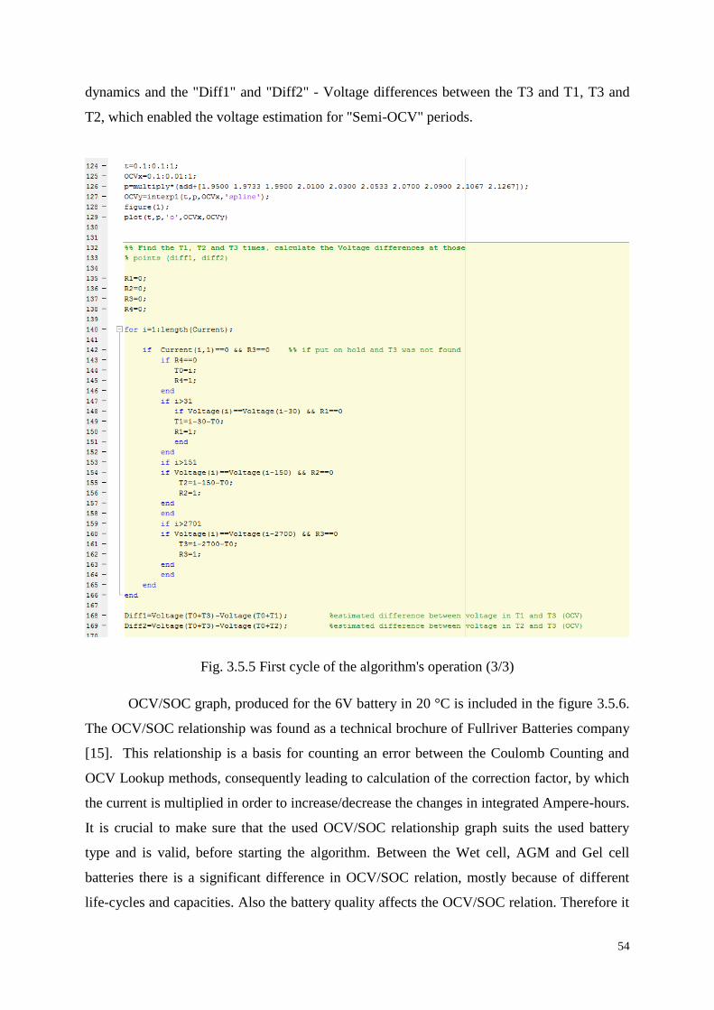
54

dynamics and the "Diff1" and "Diff2" - Voltage differences between the T3 and T1, T3 and

T2, which enabled the voltage estimation for "Semi-OCV" periods.


OCV/SOC graph, produced for the 6V battery in 20 °C is included in the figure 3.5.6.

The OCV/SOC relationship was found as a technical brochure of Fullriver Batteries company

[15]. This relationship is a basis for counting an error between the Coulomb Counting and

OCV Lookup methods, consequently leading to calculation of the correction factor, by which

the current is multiplied in order to increase/decrease the changes in integrated Ampere-hours.

It is crucial to make sure that the used OCV/SOC relationship graph suits the used battery

type and is valid, before starting the algorithm. Between the Wet cell, AGM and Gel cell

batteries there is a significant difference in OCV/SOC relation, mostly because of different

life-cycles and capacities. Also the battery quality affects the OCV/SOC relation. Therefore it

55

is recommended to ensure that we use the proper producer’s documentation before we use the

algorithm.

Fig. 3.5.6 OCV/SOC relationship for the 6V battery, working in 20 °C

Due to the need of simulating the real-time battery cycle, the main part of the

algorithm was created and implemented in MatLab Simulink software. The overview of the

Simulink program is presented in the figure 3.5.7.

The program can be divided into 4 main parts (in colored borders - 1.green, 2.red,

3.blue, 4.yellow). Each part will be described below with the insight into subsystems and

graphs, output examples and description of the role and significance of each block.

First Part (1, green border) - responsible for unmodified coulomb counting of a

current, detecting the T1, T2 and T3 points in the present current characteristics and

creating the estimated OCV graph.

Second Part (2, red border) - the Error counter is implemented in this part, using the

T1-T3, Voltage, Current, SOC (Ah) and SOC (Ah modified with factor). It compares

the SOC, giving the error value and then translates it into Ah number to be added

within the next hour of the discharge.

Third part (3, blue border) - includes pure algebraic operations of counting the

correction factor and deciding when it should be multiplied by the actual current

56

Fourth part (4, yellow border) - acts as a modified Ah counter, closing the feedback

loop of a modified SOC value with reduced error.

Fig. 3.5.7 Overview of the algorithm in MatLab Simulink.

In order to make the program logic more understandable, each subsystem will be

opened, described and its output presented, along with all necessary comments on it in order

to be re-implemented in any chosen programming language. Beginning with the first part

(green) from the figure 3.5.7. - the "SOC Counter" block is presented in the figure 3.5.8.

The SOC Counter is a typical Coulomb Counter. Having a current value as an input,

integrating it over time and dividing per 1800 (each sample is taken every 2 seconds of a real

time, making 1800 samples equivalent of 3600 seconds, which is 1 hour) enables the

algorithm to represent the number of Ampere-hours drawn from the battery. The next step is

dividing this number by "Nominal Capacity" of a battery, which - in case of the new battery -

is the operator's input as a number of Capacity (in Ampere-Hours, typically for C10

Discharging current). In the case of used battery it should be the State of Health multiplied by

the Nominal Capacity. The output of the divide block is a Depth of Discharge, so it has to be

subtracted from 1 to represent the State of Charge. The output value of this block is a SOC

over time chart, example of which is presented in the figure 3.5.9.

57

Fig. 3.5.8 "SOC Counter" block, responsible for coulomb counting.

Fig. 3.5.9 Example of SOC Counter output graph - the SOC changes over time during the

typical discharge.

The next part in the algorithm is formed as a series of 3 similar subsystems, called

"Detect the Tx point". "Detect the T1 point" is pictured in the figure 3.5.10

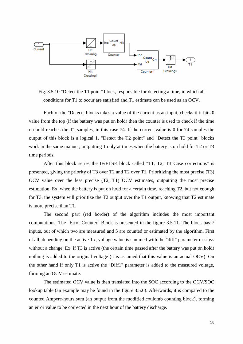
58

Fig. 3.5.10 "Detect the T1 point" block, responsible for detecting a time, in which all

conditions for T1 to occur are satisfied and T1 estimate can be used as an OCV.

Each of the "Detect" blocks takes a value of the current as an input, checks if it hits 0

value from the top (if the battery was put on hold) then the counter is used to check if the time

on hold reaches the T1 samples, in this case 74. If the current value is 0 for 74 samples the

output of this block is a logical 1. "Detect the T2 point" and "Detect the T3 point" blocks

work in the same manner, outputting 1 only at times when the battery is on hold for T2 or T3

time periods.

After this block series the IF/ELSE block called "T1, T2, T3 Case corrections" is

presented, giving the priority of T3 over T2 and T2 over T1. Prioritizing the most precise (T3)

OCV value over the less precise (T2, T1) OCV estimates, outputting the most precise

estimation. Ex. when the battery is put on hold for a certain time, reaching T2, but not enough

for T3, the system will prioritize the T2 output over the T1 output, knowing that T2 estimate

is more precise than T1.

The second part (red border) of the algorithm includes the most important

computations. The "Error Counter" Block is presented in the figure 3.5.11. The block has 7

inputs, out of which two are measured and 5 are counted or estimated by the algorithm. First

of all, depending on the active Tx, voltage value is summed with the "diff" parameter or stays

without a change. Ex. if T3 is active (the certain time passed after the battery was put on hold)

nothing is added to the original voltage (it is assumed that this value is an actual OCV). On

the other hand If only T1 is active the "Diff1" parameter is added to the measured voltage,

forming an OCV estimate.

The estimated OCV value is then translated into the SOC according to the OCV/SOC

lookup table (an example may be found in the figure 3.5.6). Afterwards, it is compared to the

counted Ampere-hours sum (an output from the modified coulomb counting block), forming

an error value to be corrected in the next hour of the battery discharge.

59

Fig. 3.5.11 "Error Counter" block, responsible for comparing the SOC counted by coulomb

counter and the more precise - SOC counted by translating OCV to SOC.

To give a better insight into the "Error Counter" operations, an example of its output is

presented as a graph in the figure 3.5.12. Although the graph is drawn continuously, only few

of the values (highlighted with the red circles) are taken into consideration by the algorithm.

Note that the variable part of the graph pictures the moments, in which the current is being

drawn, i.e. all three T1, T2 and T3 times are inactive and thus there is no way to estimate the

OCV. At those times, the previously counted correction factor is active, affecting the error

from the last discharge period. The error value will be discussed more deeply, along the rest

of the results in the next chapter.

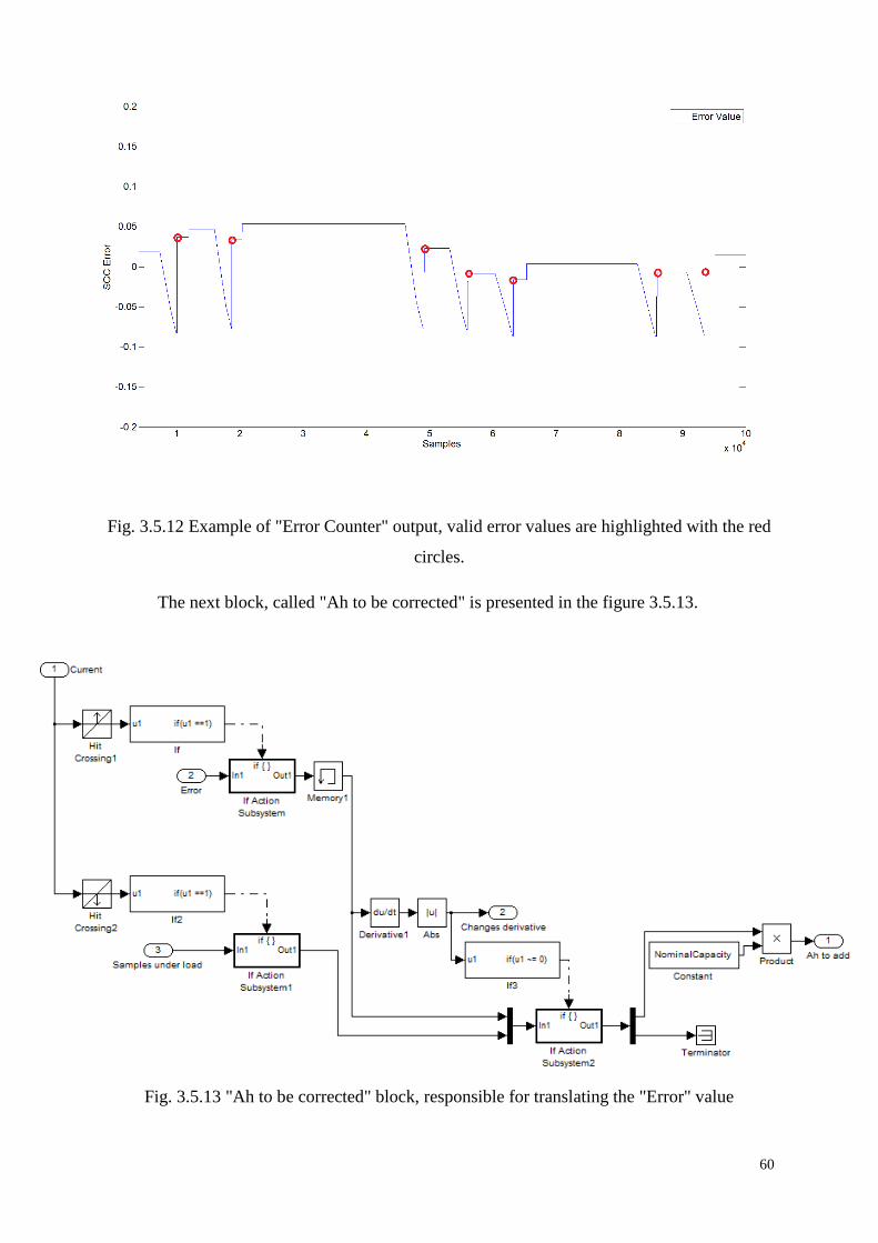
60

Fig. 3.5.12 Example of "Error Counter" output, valid error values are highlighted with the red

circles.

The next block, called "Ah to be corrected" is presented in the figure 3.5.13.

Fig. 3.5.13 "Ah to be corrected" block, responsible for translating the "Error" value

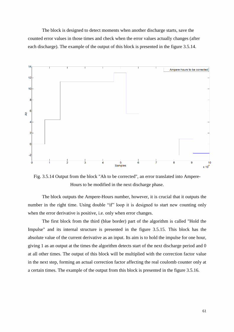
61

The block is designed to detect moments when another discharge starts, save the

counted error values in those times and check when the error values actually changes (after

each discharge). The example of the output of this block is presented in the figure 3.5.14.

Fig. 3.5.14 Output from the block "Ah to be corrected", an error translated into Ampere-

Hours to be modified in the next discharge phase.

The block outputs the Ampere-Hours number, however, it is crucial that it outputs the

number in the right time. Using double “if” loop it is designed to start new counting only

when the error derivative is positive, i.e. only when error changes.

The first block from the third (blue border) part of the algorithm is called "Hold the

Impulse" and its internal structure is presented in the figure 3.5.15. This block has the

absolute value of the current derivative as an input. Its aim is to hold the impulse for one hour,

giving 1 as an output at the times the algorithm detects start of the next discharge period and 0

at all other times. The output of this block will be multiplied with the correction factor value

in the next step, forming an actual correction factor affecting the real coulomb counter only at

a certain times. The example of the output from this block is presented in the figure 3.5.16.

62

Fig. 3.5.15 "Hold the Impulse" block, used to detect the impulse of error's change and hold it

from another discharge start for one hour.

Fig. 3.5.16 Example of an output from the "Hold the Impulse" block

As may be seen above, the impulses are held for 1 hour - 1800 samples from the

impulse, denoting the start of another discharge phase. The block parallel to this one is called

"Correction Factor" and must not be underestimated. It translates the "Ah to be corrected"

output into the actual factor, by which the current value should be multiplied in order to

reduce the coulomb counting error. The internal structure of the "Correction Factor" block is

presented in the figure 3.5.17. Its purpose is a practical realization of the previously

mentioned Correction Factor equation by dividing the sum of Ah to be corrected and the

Average Current by the Average Current itself. The factor has values of over 1 if there is a

63

need to speed up the coulomb counting (the error is positive) and the values below 1 if there is

a need to slow down the counter (the error is negative). Example of an output from this block

is presented in the figure 3.5.18.

Fig. 3.5.17 "Correction Factor" block.

Fig. 3.5.18 Example of an output from the "Correction Factor" block.

The outputs from the previous 2 blocks are multiplied, forming a vector with the

correct values of the Factor placed at correct times. Multiplied outputs are presented in the

figure 3.5.19.

After this step, the factor is ready to be multiplied by the measured current value. The

most important block from the fourth (yellow border) part of the algorithm is called

"Modified SOC Counter". Its internal structure is presented in the figure 3.5.20. This block

closes the feedback loop of an algorithm, forming next, corrected input (SOC value) for the

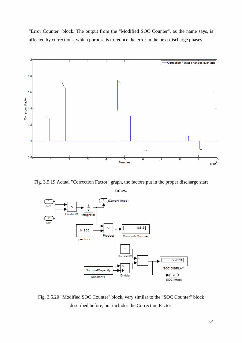
64

"Error Counter" block. The output from the "Modified SOC Counter", as the name says, is

affected by corrections, which purpose is to reduce the error in the next discharge phases.

Fig. 3.5.19 Actual "Correction Factor" graph, the factors put in the proper discharge start

times.

Fig. 3.5.20 "Modified SOC Counter" block, very similar to the "SOC Counter" block

described before, but includes the Correction Factor.

65

The example of "Modified SOC Counter" output is presented in the figure 3.5.21.

Fig. 3.5.21 Output from the "Modified SOC Counter" block, comparing to the "SOC Counter"

block. The current values are visibly modified, causing the counter to accelerate or decelerate

the counting.

This chapter will be concluded in chapter 4 "Tests" as all the results are presented there. Both

program parts are attached to this Thesis in the same form as they appear in the paper.

66

3.5.3. SOH estimation

In this section a possible implementation of an SOH estimation technique will be

presented. The designed method would greatly benefit from the addition of state of health

estimation. In the current state the method uses nominal capacity of the battery in the

calculations which will result in error increase in the long term use. The possible

implementation will be presented as an integral part of the designed method. Firstly, a

flowchart of the algorithm will be presented in figure 3.5.22:

Fig. 3.5.22 The SOH estimation algorithm flowchart

The time it takes for the battery’s terminal voltage to stabilize and reflect the open

circuit voltage may vary depending on the battery type. In the project presented in this paper it

is equal to 2 hours. Measured voltage is then subtracted by the OCV of a fully charged and at

100% SOH battery. In the case of 6V lead-acid battery the value is equal to 6.40 V. The

difference of voltages at 100 % and 0% SOC for 100% SOH is calculated only once, at the

first cycle. It is calculated based on the OCV/SOC curve presented and described in the

section 3.5.1 in the figure 3.5.6. The division of the aforementioned values results in a SOH

correction factor, which is then multiplied by nominal capacity. The calculated SOH value is

then used in Ah counting, decreasing the error caused by aging effects of the battery.

67

Fig. 3.5.6 OCV/SOC relationship for the 6V battery, working in 20 °C

It is important to note that the SOH algorithm will update only when the battery is

fully charged after the discharge cycle. Moreover, the time required for the terminal voltage to

reach the value of OCV may differ depending on the battery. However, if the aforementioned

requirements are met, the presented method is a simple and effective solution. The presented

SOH estimation method can also be easily fit into the designed method as all of the necessary

variables are available. Possible implementation of the SOH estimation is presented in figure

3.5.23:

Fig. 3.5.23 "SOC Counter" block, responsible for coulomb counting with the improvement as

a pre-counted gain SOH factor.

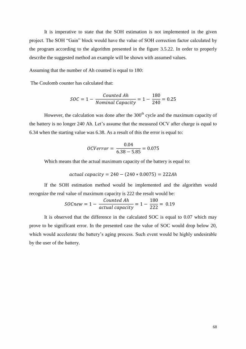
68

It is imperative to state that the SOH estimation is not implemented in the given

project. The SOH “Gain” block would have the value of SOH correction factor calculated by

the program according to the algorithm presented in the figure 3.5.22. In order to properly

describe the suggested method an example will be shown with assumed values.

Assuming that the number of Ah counted is equal to 180:

The Coulomb counter has calculated that:

However, the calculation was done after the 300th

cycle and the maximum capacity of

the battery is no longer 240 Ah. Let’s assume that the measured OCV after charge is equal to

6.34 when the starting value was 6.38. As a result of this the error is equal to:

Which means that the actual maximum capacity of the battery is equal to:

If the SOH estimation method would be implemented and the algorithm would

recognize the real value of maximum capacity is 222 the result would be:

It is observed that the difference in the calculated SOC is equal to 0.07 which may

prove to be significant error. In the presented case the value of SOC would drop below 20,

which would accelerate the battery’s aging process. Such event would be highly undesirable

by the user of the battery.

69

4. Tests

4.1. Reference method

In this subsection results of the tests conducted on the reference method will be

presented. The current and voltage curves used for calculation of the OCV by the method are

presented in the figures 4.1.1 and 4.1.2 respectively.

Fig. 4.1.1 Measured Current

Fig. 4.1.2 Measured Voltage

70

In the figure 4.1.3 the calculated OCV in regard to terminal voltage is presented:

Fig. 4.1.3 Terminal voltage and calculated OCV

It is observed that the error in calculation of the OCV is increasing with the time. In

order to properly explain the reasons behind such occurrence a few theoretical facts regarding

the method must be brought. Firstly, the system in the form:

is observable only when the current Ib(t) is not constant. This phenomenon is observed in the

presented figure, when the OCV remains at the same value for periods of time. During the

period of 40 minutes after the current stopped flowing, the value of terminal voltage should be

close to the real open circuit voltage. The measurements were taken every 2 seconds, which

means that the 40 minutes equal ~1200 samples in the presented figure. It can be observed

that the values of calculated OCV and terminal voltage after 1200 samples without current

differ significantly. However, it is imperative to notice that in the article “Estimating the State

of Charge of a Battery” by John Chiasson and Baskar Vairamohan it is stated that the method

71

requires resetting to work properly. It is also worth noting that presented in the paper

experiments were carried out with much shorter times (1000 s).

Figures 4.1.4, 4.1.5 and 4.1.6 present the calculated OCV if the method is reset twice,

at equal intervals of 33366 samples:

Fig. 4.1.4 Calculated OCV and terminal voltage in the first 33366 samplesFig. 4.1.5

Calculated OCV and terminal voltage after the first reset of the method

72

Fig. 4.1.6 Calculated OCV and terminal voltage after the second reset of the method

It is observed that resetting the algorithm significantly improves the precision of OCV

calculation. However, the error between the terminal voltage value reaching real OCV and the

calculated one in figure 4.1.5 is equal to around 0.1 V which still indicates a low precision of

the estimate. The big disadvantage of the presented method at its current state is the necessity

to manually choose the reset times of the method.

In order to calculate SOC based on the estimated value of OCV a curve is to be used

which was presented in the figure 3.5.6 in the section 3.5.2 of this paper. Calculated SOC is

presented in figure 4.1.7:

Fig. 4.1.7 SOC calculated by the reference method

73

In the presented figure, the values real SOC values are denoted by the 'x' signs. Those

points were derived from the real OCV (the voltage values which are not changing for at least

2700 samples when the battery is put on hold). The curve was cut off after 55000 samples as

the error between the calculated and real SOC became too high. It is imperative to state once

again that the method requires resetting in order to work properly. Obtained results might

differ from those achieved in the paper wrote by John Chiasson. However, those presented in

the aforementioned paper show that the method was reset at least two times in the time span

of 1000 seconds. It was shown that the method cannot handle calculation of OCV over longer

period of time without frequent resets. Presented method could benefit greatly from the

correction factor described in the designed method section.

The comparison of the reference method and Coulomb Counting is presented in the

figure 4.1.8.

Fig. 4.1.8 Comparison of the reference method and Coulomb Counting

The comparison was done with the Coulomb Counting as both of these methods are

used to estimate the OCV when a battery is charging or discharging. The experiment indicates

that in the long run (more than 10 hours) both the Coulomb Counting as well as the reference

method yield high difference compared to measured open circuit voltage points. I.e. more

than 0.1 volt which corresponds to more than 10% difference in SOC. In the shorter time

perspective (less than 10 hours) the difference for the comparison estimation method is less

than 5% and the Coulomb Countng less than 10%.

74

The comparison method experiment indicate that the estimation method improve

Coulomb Counting and seems to be close to fulfilling Micropower’s requirements.

4.2. Designed Algorithm

Both comparison and the coulomb counting methods could be improved by the use of

periods when no current is drawn, however it has been chosen to show the improvement of

the coulomb counting as it is more widely used in the industry and already implemented in a

Micropower measurement tool.

In this part of the chapter, precision of designed algorithm will be evaluated on a

sample measured current (Figure 4.1.1) and voltage (Figure 4.1.2) graphs as inputs. To keep

the consistence all the graphs presenting different variables from chapter 3, “Implementation”

were derived using the same voltage and current graphs.

The graph showing the changes in SOC based on regular coulomb counting and the

desired SOC based on OCV is presented in the figure 4.2.1.

Fig. 4.2.1 Unmodified Coulomb Counting SOC compared to SOC based on OCV

75

The original Coulomb Counting generates an unacceptable error in most of the points

when OCV can be measured or estimated. The differences between both SOC measurements

observed in the figure 4.2.1 show the reason why there was a need to implement the algorithm

described in this Thesis. Without a feedback, the original, unmodified coulomb counting

blindly integrates the measured current values. Not only this procedure is very dependent on

the sampling time and a data collection device, but also progressively adds the variable

measurement error. The error varies between 2% and 12% during the simulation. For the

following reasons it is rather unpredictable algorithm, which needs improvement.

The results of algorithm improvement, presented as changes in SOC based on the

improved coulomb counting along with the desired SOC, based on OCV are presented in the

figure 4.2.2.

Fig. 4.2.2 Improved Coulomb Counting SOC compared to SOC based on OCV

According to the regressive corrections foundation of the algorithm, the error seen as a

difference between the red line and the black crosses on the chart is greater at start and

reduced with the further discharge periods. It is conspicuous that the SOC values obtained

with use of the designed improved coulomb counting algorithm are much closer to the desired

SOC/OCV points. The error values in all highlighted moments vary between 1 and 5% and

are reduced over time. With the exception when the OCV estimate does not manage to reach

the real OCV value, produces increased error, but corrects itself within next 100 samples. The

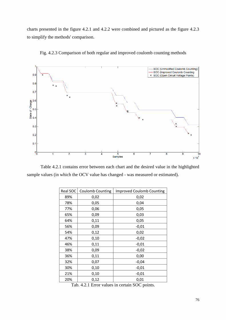
76

charts presented in the figure 4.2.1 and 4.2.2 were combined and pictured as the figure 4.2.3

to simplify the methods' comparison.

Fig. 4.2.3 Comparison of both regular and improved coulomb counting methods

Table 4.2.1 contains error between each chart and the desired value in the highlighted

sample values (in which the OCV value has changed - was measured or estimated).

Real SOC Coulomb Counting Improved Coulomb Counting

89% 0,02 0,02

78% 0,05 0,04

77% 0,06 0,05

65% 0,09 0,03

64% 0,11 0,05

56% 0,09 -0,01

54% 0,12 0,02

47% 0,10 -0,02

46% 0,11 -0,01

38% 0,09 -0,02

36% 0,11 0,00

32% 0,07 -0,04

30% 0,10 -0,01

21% 0,10 -0,01

20% 0,12 0,01

Tab. 4.2.1 Error values in certain SOC points.

77

According to the table 4.2.1, the designed algorithm produces reasonably low error

values during the whole discharge period, providing the forklift operator with a dependable

estimate of the battery state of charge in any time of the discharge.

5. Conclusions and future work

5.1. Conclusions

The purpose of the presented thesis was to design an SOC estimation algorithm which

would fulfill requirements presented in the section 3.1. All of the mentioned requirements

were met with certain limitations. Firstly, the SOC error is below 5% which was shown in the

table 4.2.1. However, unless the changes proposed in section 3.5.3 are implemented, precision

level will decrease with the battery aging. No parameterization is required for the algorithm to

start, however, its precision is highly dependent on the frequency of the discharge breaks’

occurrence. All of the available measured variables are used. The only manual input required

from the operator is the nominal capacity of the battery in the beginning of algorithm

operation. Although the algorithm is implemented in MatLab SimuLink environment, it may

be easily transitioned into C programming language.

The results of the reference method presented in the thesis justifies the use of black-

box approach in the algorithm’s design. The method created by John Chiasson and Baskar

Vairamohan was implemented with consideration of the aforementioned requirements. The

comparison method in the time interval less than 10 hours almost fulfills the requirement of

5% maximum error. Higher precision could be achieved with addition of proper

parameterization, optimization and resetting of the algorithm. However, the purpose of the

Thesis was to design an algorithm with the minimum input from the operator which excludes

the reference method. Presented results confirm that for the specific purpose specified in this

thesis, black-box modeling yields better results.

79

5.2. Future work

Even though all the primary objectives were achieved there is still plenty of room for

improvement. The main weakness of the Improved Coulomb Counting algorithm is

undoubtedly the need of the discharge breaks during its work, as only then the error value can

be counted. Naturally, without error value, the correction factor cannot be counted and the flat

coulomb counting may not be evaluated. In recent state the algorithm is aimed exclusively at

HEVs and EVs, which typically have several breaks during their operation cycle. The idea of

using so called "Current Profiles" is a way to extend the algorithm's applications and broaden

its functionality.

In shortage: the current profiles would exclude the necessity of breaks in the battery

discharge, by saving the information regarding the previous:

discharge period lengths

average current values throughout the discharge periods

the error produced in those periods

Saved as a vector, ex. [200, 14, 0,02] ([samples, Amperes, error value]) the information

might be stored (forming a database), corrected over time and used if there is a constant

discharge for at least two hours. Such solution would exclude the need of stopping the

discharge during the operation cycle, extending the algorithm applications into many different

regions.

The current profiles idea was discussed and seriously taken into consideration, but in

the end it was not implemented in this thesis. However the solution is advised to be

implemented as soon as there is a need for using the algorithm in any other applications than

mentioned in this thesis as this could be done by identifying an exponential function for the

OCV recovery and stored as just a couple of parameters.

s

80

6. References

1. K. M. Abraham, Z. Jiang, ”A polymer Eelctrolyte-Based Rechargeable Lithium/Oxygen

Battery”, Journal of the Electrochemical Society, Vol. 143, 1996

2. Matthew Barth, Jie Dy, Jay Farell, Shuo Pang, ”Battery state-of-charge estimation”,

Proceedings of the American Control Conference, Vol. 2, June 2001

3. Massimo Ceraolo, “New Dynamical Models of Lead-Acid Baatteries”, IEEE Transactions

On Power Systems, Vol. 15, NO. 4, November 2000

4. D. Sutanto, H.L. Chan, “ A New Battery Model for use with Battery Energy Storage

Systems and Electric Vehicles Power Systems”, Power Engineering Society Winter Meeting,

January 2000

5. John Chiasson, Baskar Variamohan, “Estimating the State of Charge of a Battery”,

Transactions on Control Systems Technology, Vol. 13, NO. 3, May 2005

6. D.Jaya Deepti, V. Ramanarayanan, “State of Charge of Lead Acid Battery”, Proceedings of

India International Conference on Power Electronics, 2006

7. Francisco M. González-Longatt, “Circuit Based Battery Models: A Review”, 2DO

Congreso Iberoamericano De Estudiantes De IngenierÍa Eléctrica, 2006

8. James A Gucinski, David F Smith, ”Synthetic silver oxide and mercury-free zinc electrode

for silver-zinc reserve batteries”, Journal of Power Sources, Vol. 80, July 1999

9. Yao-Feng Huang, Chin-Sien Moo, Kong-Soon Ng, Yao-Ching Hsieh, ”An Enhanced

Coulomb Counting Method for Estimating State-of-Charge and State-of-Health of Lead-Acid

Batteries”, Hsieh INTELEC 2009 -31st International Telecommunications Energy Conference,

2009

10. Robyn A. Jackey, ”A simple, Effective Lead-Acid Battery Modeling Process for Electrical

System Component Selection”, SAE Paper, 2007

11. Hurng-Liahng Jou, Jinn-Chang Wu, Yu-Hua Sun, “Aging Estimation Method for Lead-

Acid Battery”, IEEE Transactions On Energy Conversion, Vol. 26, NO. 1, March 2011\

12. H.A. Kiehne, “Battery Technology Handbook, Second Edition”, Taylor & Francis Group,

August 2003

13. Dirk Uwe Sauer, Heinz Wenzl, “ Comparison of different approaches for lifetime

prediction of electrochemical systems-Using lead-acid batteries as example”, Journal of

Power Sources, Vol. 176, NO. 2, February 2008

14. http://www.batterycouncil.org

81

15. Fullriver battery company, “Performance Characteristics – DC Series Batteries”:

http://www.fullriverdcbattery.com/media/pdf/technical/performance_characteristics.pdf

16. Barrie Lawson, “State of Charge (SOC) Determination”, Woodbank Communications,

Electropaedia: http://www.mpoweruk.com/soc.htm

17. Trojan Battery Company, “Comparing deep-cycle flooded batteries to VRLA Batteries”,

http://www.trojanbatteryre.com/Tech_Support/ComparingFlood2VRLA.html

18. A project of Battery Council International, Lead-Acid Battery info, ”Lead-Acid battery

uses”: http://www.leadacidbatteryinfo.org/lead-acid-battery-uses.htm

19. Battery University – How to measure state of charge

http://batteryuniversity.com/learn/article/how_to_measure_state_of_charge

http://www.fullriverdcbattery.com/media/pdf/technical/performance_characteristics.pdf

http://www.mpoweruk.com/soc.htm

http://www.trojanbatteryre.com/Tech_Support/ComparingFlood2VRLA.html

http://www.leadacidbatteryinfo.org/lead-acid-battery-uses.htm

http://batteryuniversity.com/learn/article/how_to_measure_state_of_charge

Development of an algorithm for estimating Lead-Acid ...830232/FULLTEXT01.pdf · Development of an...

Documents

Transcript of Development of an algorithm for estimating Lead-Acid ...830232/FULLTEXT01.pdf · Development of an...