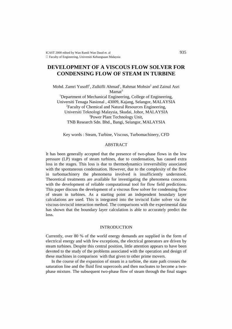
ICAST 2000 edited by Wan Ramli Wan Daud et. al 935 Faculty of Engineering, Universiti Kebangsaan Malaysia

DEVELOPMENT OF A VISCOUS FLOW SOLVER FORCONDENSING FLOW OF STEAM IN TURBINE

Mohd. Zamri Yusoff1, Zulkifli Ahmad1, Rahmat Mohsin2 and Zainul AsriMamat3

1Department of Mechanical Engineering, College of Engineering,Universiti Tenaga Nasional , 43009, Kajang, Selangor, MALAYSIA

2Faculty of Chemical and Natural Resources Engineering,Universiti Teknologi Malaysia, Skudai, Johor, MALAYSIA

3Power Plant Technology Unit,TNB Research Sdn. Bhd., Bangi, Selangor, MALAYSIA

Key words : Steam, Turbine, Viscous, Turbomachinery, CFD

ABSTRACT

It has been generally accepted that the presence of two-phase flows in the lowpressure (LP) stages of steam turbines, due to condensation, has caused extraloss in the stages. This loss is due to thermodynamics irreversibility associatedwith the spontaneous condensation. However, due to the complexity of the flowin turbomachinery the phenomena involved is insufficiently understood.Theoretical treatments are available for investigating the phenomena concernswith the development of reliable computational tool for flow field predictions.This paper discuss the development of a viscous flow solver for condensing flowof steam in turbines. As a starting point an independent boundary layercalculations are used. This is integrated into the inviscid Euler solver via theviscous-inviscid interaction method. The comparisons with the experimental datahas shown that the boundary layer calculation is able to accurately predict theloss.

INTRODUCTION

Currently, over 80 % of the world energy demands are supplied in the form ofelectrical energy and with few exceptions, the electrical generators are driven bysteam turbines. Despite this central position, little attention appears to have beendevoted to the study of the problems associated with the operation and design ofthese machines in comparison with that given to other prime movers.

In the course of the expansion of steam in a turbine, the state path crosses thesaturation line and the fluid first supercools and then nucleates to become a two-phase mixture. The subsequent two-phase flow of steam through the final stages

936

of turbines poses a number of problems which are not encountered in otherturbomachines. In conventional power plant, the wetness levels in the last fewstages of the LP turbines can be as high as 10 - 12 %. It is agreed in the literaturethat the nucleating and wet stages of steam turbines are less efficient than thoserunning with superheated steam. This reduction in efficiency is attributedcollectively to wetness loss, but the mechanisms which give rise to them areinsufficiently understood.

Many research efforts, both experimental and theoretical, have been done inorder to improve the efficiency of LP turbine running with wet steam e.g. Zamri(1997), Mamat (1996), White and Young (1994). The theoretical work solves thephysical governing equations numerically using computer in order to simulatethe real flow process in steam turbine, while the experimental data providemeans for validating the theoretical predictions. These are aimed atunderstanding the mechanisms that cause the extra losses and use the knowledgeto design better turbine blade profiles.

Flow in real turbomachines is very complex being three-dimensional,unsteady, viscous and turbulent. However, in many cases, considerable physicalinsights into the phenomena involved can be gained by simplifying the flow. Wu(1952) showed that, the general three-dimensional flow within a turbomachinecan be reasonably described by a combination of two-dimensional solutions intwo different planes. The first family is referred to as S1 or blade-to-blade planeand the second one as S2 or meridional plane. The solutions on S2 plane provideinformation about the mean flow through the turbine, while S1 solutions giveinformation about flow behaviour round individual blade sections. Instead ofsolving the full three-dimensional equations, considerable saving can be gainedby solving the two-dimensional equations and iterate between the two planes.

A two-dimensional blade-to-blade, computer program for two-phasecondensing flow of steam has been recently developed [Zamri (1997 & 1998),Zamri et al. (1998)]. The program solves the two-dimensional time-dependentEuler equations using second-order accurate cell-vertex finite volume integrationtogether with the fourth order Runge-Kutta time stepping. To take into accountof the two-phase effect, the governing equations are coupled with the equationsdescribing the droplet formation and growth. The applications of the solver tocondensing flow of steam in cascade of turbine bladings have shown very goodagreement with the experimental data in term of condensation loss and overallblade pressure distributions. However, the program cannot predict the extralosses due to viscous effect which has been found experimentally to besignificant in transonic conditions [Mamat (1996)].

As a first step towards developing a fully viscous solver, an independentboundary layer calculations subroutine is used. This program is coupled with theEuler solver by using the viscous-inviscid integral boundary layer interactionmethod. In this paper the numerical formulations which are used to solve the

937

∫ −−=ΩS

dxGdyFtw )(

∂∂

0EVV

wy

x

ρρρρ

=

0

2

HVVV

PV

V

F

x

yx

x

x

ρρρ

ρ

+=

0

2

HVPV

VVV

G

y

y

xy

y

ρρ

ρρ

+=

governing equations will be discussed. This will be follwed by the discussion onthe Integral viscous-inviscid integral boundary layer method. Finally theprogram, will be applied to condensing flows in cascade of turbine blades andthe results will be compared with the experimental measurements.

NUMERICAL FORMULATIONS

The governing equations employed are the time dependent Euler equations. Themain flow governing equations cast in the finite volume formulation in x-ycartesian coordinates system is : -

where

Ω is the volume of the small element with perimeter S as shown inFIGURE 1. The small element shown is one of the finite volumes which areformed by the intersection of quasi-streamlines and quasi-orthogonal lines. Theflow variables are stored at the cell vertices. In this paper, only a briefdescription of the numerical formulations will be given. Detail descriptions canbe obtained in Zamri (1997 and 1998). The above equations are solvedsimultaneously for each finite cell volume using a time marching method.

The spatial integration is done using central discretization which is ofsecond order accuracy. A blend of second and fourth order artificial dissipationswith pressure switch are added to the residuals prior to the time integration toremove wiggles from the solution. The temporal integration is done using thefourth order accurate, 4 stage Runge Kutta time stepping. To speed up theconvergence, 3 types of convergence acceleration schemes are employed namely,local time-stepping, enthalpy damping and implicit residual averaging.

At inlet boundary, the total pressure, total temperature and flow angle arefixed while the static pressure is extrapolated from the interior. At exit, if the exitflow is subsonic, only the static pressure is fixed, while total pressure, totaltemperature and flow angle are extrapolated from the interior. If the exit flow issupersonic, all four variables are extrapolated from the interior. The periodicitycondition on the bounding streamlines, upstream and downstream of the bladerow, is easily satisfied by treating the calculating points on each of the boundingstreamline as if they were interior ones. At the solid boundary, normal fluxes areset to zero.

(1)

(2)

938

N

To apply the above conservation equations and solution procedures to the twophase flows, the equations have to be combined with the equations describing thedroplet formation and growth and solved simultaneously. The equation fordescribing the rate of nucleation of the droplet per unit volume is

( )

( )

∆−+

=GL

GGsrst kT

GTm

qv

J*

3 exp2

11

ρρρ

πσ

The equation for the rate of growth of the droplet is given by

drdt L

T T

r lL

L G=−

+

λρ 159.

_

The two sequences of calculations are carried out separately, but it isessential that the coupling between them be exact. This is achieved by theintroduction of the wetness fraction, w, into the expression for mixture enthalpyh and density ρ to yield : -

h w h whG L= − +( )1and

1 1 1 1ρ ρ ρ

= − +( )w wG L

The wetness fraction, w, in turn may be expressed as : -

w r N L= 43

3π ρ

where is the number of droplet per unit mass of mixture. The additionalinformation necessary is the equation describing the properties of the liquid andvapor phases. The equation of state adopted for the vapor phase is :

PRT

BG G

Gρρ= +1

where B is the second virial coefficient and thermodynamic properties of steamare calculated from mutually consistent relationships. The above systems ofequations are sufficient to describe the flow completely.

INTEGRAL BOUNDARY LAYER METHOD

In the viscous-inviscid interaction method the viscous effects are assumed to beconcentrated in the boundary layers adjacent to the blade surfaces and the mainflow-field is regarded as inviscid and described by the Euler equations. The

(3)

(4)

(5)

(6)

(7)

(8)

939

boundary layer subroutine covers the laminar boundary layers, natural transitionand transition through bubble separation, turbulent boundary layers and wakes.

Laminar Boundary Layer

The method of Thwaites (1949) has been adopted due to its simplicity andadequate accuracy. This method consists of the numerical integration of themomentum integral equation, using auxiliary relationships for skin friction andshape factor as functions of pressure gradient parameter, Λ. Thwaites showedthat the momentum thickness, θ , is given by : -

∆θ ν 2 = 0 456

5

0

.

VV dx

ee

x

∫ (9)

where, the bar over Ve denotes the average value over an increment ∆x.In order to calculate the skin friction coefficient and the displacement

thickness, the modified expressions for L(Λ) and H(Λ) as given by Cebeci (1977)are used. δ ∗ and Cf can be evaluated as : -

δ θ∗ = H (10)

( )CV V

Vy V

Lfwall

e ee y e

= =

= τ

ρ

ν ∂∂

νθ1

2

2 22

20

=

Λ (11)

Laminar-Turbulent Transition

Boundary layer transition from laminar to turbulent flow can occur either bynatural transition or laminar separation bubble ending in reattachment as aturbulent boundary layer.

In natural transition, there is a gradual increase in the proportion of the flowwhich is turbulent at any instant (intermitency) from zero to one. Naturaltransition is assumed to occur when the momentum thickness Reynolds numberreaches a critical value, which is a function of the pressure gradient parameterand the turbulence level.

In a laminar separation bubble, the laminar boundary layer separates andforms a laminar free shear layer which eventually undergoes transition toturbulence. The turbulent free shear layer gains sufficiently high energy fluidfrom the free-stream by diffusion to reattach as a turbulent boundary layer.Bubble transition occurs if the pressure gradient parameter, Λ , falls below -0.09.The bubble length and the condition on reattachment are determined by twoempirical correlations by Horton (1968). The flow was assumed to undergotransition to turbulence at the start of bubble separation. It is also assumed that

940

boundary layer transition occurs instantaneously upon interaction with ashockwave.

Turbulent Boundary Layer

The lag-entrainment method originated by Head (1958) is used in the treatmentof turbulent boundary layers. This method employs three differential equations;the momentum integral equation, the entrainment equation and an equationdescribing the streamwise rate of change of entrainment coefficient. The firsttwo equations are those used in Head’s original treatment, the last one is anequation for shear stress developed by Bradshaw et al. (1967). The method alsoallows a first-order approximation for compressibility. The three equations are asfollows : -

( )ddx

CH Ma

VdVdx

fe

e

eθ θ = 2

2 2− + − (12)

( )θ θ = d Hdx

d HdH

C HC

HV

dVdxE

f

e

e

11 2

1− − +

(13)

( )θ λ θτ τ =

dCdx

FH H

C CV

dVdx

EEQ b

e

e

EQ

2 81

0

12

12.

+−

+

− +++

θV

dVdx

Ma MaMae

ee

e

e

1 0 0751 0 21 01

22

2. ..

(14)

where, Mae is free-stream Mach number, Cτ is the shear stress coefficient, λb isthe overall scaling factor and suffices EQ and 0 indicate the values inequilibrium flow and zero pressure gradient respectively.

The auxiliary relations for other boundary layer parameters; Cf, H, H1,d H /dH1, Cτ and F in the above equations are that given by Green et al. (1973).Equilibrium flows are defined as those in which the shape of the velocity andshear stress profiles in the boundary layer do not vary with distance, x.Therefore, throughout the flow, dH/dx and d(Cτ)max/dx are both zero. Theauxiliary equations for the equilibrium quantities are taken from expressionsrecommended by Green et al. (1973).

The boundary layer growth is calculated by the simultaneous forwardintegration of the three differential equations using Runge-Kutta technique forthe three independent variables, momentum thickness, θ, transformed shapefactor, H and the entrainment coefficient, CE .The distribution of displacementthickness, δ ∗ and other boundary layer parameters are obtained from these.

941

Treatment of Wake

The basic equations governing the flow in boundary layers are equally applicableto wakes. Thus, the treatment of attached boundary layers described above canbe applied to wakes with only minor modifications. The skin friction, Cf is set tozero and the overall scaling factor, λb is halved.

NUMERICAL PROCEDURES

In the viscous-inviscid interaction procedure, the inviscid free-stream flow for agiven blade geometry is first determined and then the boundary layerdisplacement thickness corresponding to the blade inviscid velocity distributionis evaluated. The displacement thickness on both suction and pressure surfacesare then added in order to modify the blade geometry. The process is thenrepeated until the solutions converge. In the numerical solution, the boundarylayer calculation is called at 400th time step and subsequently at an interval of200 time steps until the solutions converge.

The boundary layer is initially laminar around the leading edge, but thepressure distribution obtained in this region is affected by numerical errors. Forthis reason, the start of the boundary layer treatment is delayed for a distanceequivalent to about 2-3 % of the blade chord. At the starting point, the values ofθ and Cf are assumed to be zero and 0.025 respectively. This simplification haslittle effect on the accuracy because the displacement and momentum thicknessare very small in this region.

BLADE PROFILE LOSS AND WETNESS LOSS

The profile loss of a turbine blade is defined as the loss due to boundary layergrowth on the blade surface and the subsequent dissipation in the blade wake.The boundary layer loss is calculated by : -

BlPitchloss = x 1 1 100

2

− −−

∗

θδ

% (15)

where θ and δ ∗ represent the summation of their values on the suction andpressure sides at the trailing edge plane. The mixing loss is given by : -

( )Mixing

K E V V

K Eloss

x mix y mix x =

− +. .

. .%

12 100

2 2

(16)

The extra loss incurred due to two-phase effects is called thermodynamicwetness loss. The loss is due to the departure of the fluid from thermodynamicequilibrium. The latent heat of the phase change is given up to the liquid before

942

it is transferred back to the vapour. The process is thermodynamicallyirreversible. In the case of diffusion of flow or encounter with shockwave, therewill have to be some evaporation from the droplets. For this purpose, they willhave to receive heat from surrounding which will again occur irreversibly. Toestimate the magnitude of these losses a method based on the calculation ofentropy increase along the quasi-streamlines has been used. The increase in thespecific entropy of the fluid for such transfer of heat may be written as : -

∆s ds LdwT TG L

= = ∫ ∫ −

1 1 (17)

where L and w are latent heat and wetness fraction respectively. By integratingthe above expression along each the quasi-streamline up to the exit plane andtaking the pitch average, the loss can be calculated.

RESULTS

The flow solver developed was applied to condensing flows of steam overcascade of a nozzle profile. The general shape of the profile is shown inFIGURE 2. Experimental measurements have been performed by Mamat (1996)in the blow-down tunnel at the University of Birmingham, U.K. The calculationswere performed for various flow conditions similar to the experiments coveringsubsonic, sonic and supersonic dry and nucleating flows. FIGURE 3 shows themesh arrangements used. A typical flow field predictions (contours of constantdensity) for supersonic condition for dry and nucleating flows are shown inFIGURES 4 and 5 respectively. Also shown in the figures are the experimentallyobserved Mach-Zhender photographs for both cases. It can be seen that for bothcases the flow features have been predicted accurately. Comparing the dry andnucleating flow, it can be observed that the features are similar except in thethroat region. In this region the trailing edge shockwaves systems are weaker forthe nucleating flow. The reason for weaker shockwave is condensation thatoccurred in the throat region. This is shown clearly in the contours of constantwetness fraction as shown in FIGURE 6. Nucleation seems to be started aroundthe throat of the passage and the associated release of latent heat to the vaporcaused the flow to decelerate and hence producing weaker shockwave systems.In FIGURES 7 and 8 the predicted values of blade surfaces and mid-passagepressure distributions are compared with the experimental data for the dry andnucleating flows respectively. It can be seen that the agreements between themare excellent. The nucleation region signified by the knee shape in the suctionsurface pressure distribution have been predicted accurately.

The overall accuracy of the boundary layer calculations can be determined bycomparing the measured and calculated expansion efficiency. The predicted totalloss is the summation of wetness, boundary layer, mixing and shock losses. The

943

overall results obtained from all the calculations are compiled in TABLE 1. Itcan be seen that the predicted expansion efficiencies are in very close agreementwith the experimental data. It can be concluded that the boundary layercalculation is able to accurately predict the loss accurately.

CONCLUSIONS AND FUTURE WORKS

The development of the viscous flow solver for condensing flow of steam inturbine is described. As a starting point an independent boundary layercalculations are used. This is integrated with the inviscid Euler solver with theviscous-inviscid interaction method. The comparisons with the experimental datahas shown that the boundary layer calculation is able to accurately predict theloss. However, because of the nature of the viscous-inviscid interaction method,it is not possible to predict the direct interaction between the boundary layer andmain flow field such as shock boundary layer interaction. In order to predict this,direct inclusion of the viscous term including the turbulence terms into thegoverning equations are needed. The next step of the work is the inclusion ofthese terms into the governing equations. This would also open the possibility ofinvestigating the condensations in the boundary layer region.

FIGURE 1 : An Element of A Mesh FIGURE 2 : Nozzle Blade Cascade Geometry

944

NOTATIONS

Eo Total internal energyF Scaling function in skin friction lawG Gibbs free energyH Mean velocity shape factorH1 Mass flow shape factorHo Stagnation enthalpyh Specific enthalpyJ Rate of formation of critical nuclei per mass per unit timek Boltzman’s constantK.E. Kinetic energyL Latent heat ( hg - hL) or Thwaites parameterm Mass of moleculeP Static pressureq Condensation coefficientR Gas constant of vapour

FIGURE 3 : Mesh Arrangement FIGURE 4 : Constant Density Contours – Dry Flow

945

r Droplet radiuss Specific entropyT Temperaturet Timeδt Time step for the droplet growth calculationV Overall velocityρ Densityλ Thermal conductivityΛ Thwaites pressure gradient parameterτ Shear stressν Kinematics viscosity, specific volume or correction factor in

nucleation rate equationδ Overall boundary layer thickness, incremental changeδ* Displacement thicknessσ Surface tension

Subscript

G Vapour phaseL Liquid phasemax maximummix mixed valuesr Droplets Saturationst Steady state

REFERENCES

Zamri, M.Y. An improved treatment of Two-Dimensional Two-Phase Flows of Steam bya Runge-Kutta Method’, 1997, Ph.D. Thesis, Department of Manufacturing andMechanical Engineering, The University of Birmingham, U.K.

Mamat, Z.A. 1996 The Performance of a Cascade of Nozzle Turbine Blading inNucleating Steam, Ph.D. Thesis, Department of Manufacturing and MechanicalEngineering, The University of Birmingham, U.K.

White, A.J. and Young, J.B. 1994, Time Marching Method for the Prediction of Two-Dimensional, Unsteady Flow of Condensing Steam, J. Propulsion and Power, 9 (4).

Wu, Chung-Hua, 1952, A General Theory of Three-Dimensional Flow in Subsonic andSupersonic Turbomachines of Axial Radial and Mixed-Flow Types . NASA TN 2604

Mohd. Zamri Yusoff, Ibrahim Hussein, Mohd. Azree Idris, 1998 Prediction andImprovement of Steam Turbine Performance Using Computational Fluid Dynamics(CFD), Proceedings of the 1st TNB Technical Conference, Universiti Tenaga Nasional,July, 1998.

946

Mohd. Zamri Yusoff, 1998, A Two-Dimensional Time-Accurate Euler Solver for Turbo-machinery Applications, Journal of Institute of Engineers, Malaysia, 59 (3)..

Thwaites, B.,1949, Approximate Calculation of the Laminar Boundary Layer Aero.Quarterly, 1 : 245-280.

Cebeci, T. 1977 , Calculation of Laminar and Turbulent Boundary Layers for 2-d TimeDependent Flows, N.A.C.A. C.R., No. 2820.

Horton, H.P. 1968, Laminar Separation Bubbles in Two and Three DimensionalIncompressible Flow, P.h.D. Thesis, Queen Mary College, Dept. of Aero. Eng.

Head, M.R. 1958, Entrainment in Turbulent Boundary Layer, A.R.C.R. and M. No.3152, September 1958.

Bradshaw, P., Ferriss, D.H. and Atwell, N.P. 1967, Calculation of Boundary LayerDevelopment Using the Turbulent Energy Equation, J. Fluid Mech., 28 (3) : 593-616

Green, J.E., Weeks, D.J. and Brooman, J.W.F. 1973, Prediction of Turbulent BoundaryLayer and Wakes in Compressible Flow by Lag Entrainment Method, A.R.C., R. andM., No. 3791.

947

FIGURE 5 : Constant Density Contours – Nucleating Flow

FIGURE 6 : Constant Wetness Fraction Contours – Nucleating Flow

FIGURE 7 : Comparison of Measured andPredicted Surfaces and Mid Passage StaticPressure Distributions – Dry Flow

FIGURE 8 : Comparison of Measured and PredictedSurfaces and Mid Passage Static PressureDistributions – Nucleating Flow

948