Development of a Tilt Control Methodfor a Narrow Track Three Wheeled

Vehicle

Revised Paper Submitted on April 21, 2011

Authors: Dr J. Berote, Dr J. Darling and Prof. A. Plummer

Department of Mechanical EngineeringUniversity of BathBath, BA2 7AY

U.K.

Abstract

The space and weight savings provided by narrow tilting vehicles could make them a

solution to the pollution and congestion problems seen in urban environments. The

success of this new type of vehicle relies heavily on the control method used to balance

the vehicle in corners. A tilting three-wheeled vehicle was developed at the University

of Bath as part of an EU funded project. The original direct tilt control method

implemented on the prototype was shown to perform well in steady state, but rapid

transients were shown to potentially lead to instability. A new type of controller was

therefore required to reduce the load transfer across the rear axle during transient state

manoeuvres.

This paper presents a linearised model of the tilting vehicle system which is used to

optimise a new tilt controller in the frequency domain. The controller, which uses

combined steer and tilt control inputs, is shown to significantly reduce transient roll

moments compared to the previous control method. This results in a much safer and

more predictable handling characteristic.

Key Words: tilt control, handling, narrow track, tilting, three-wheeled vehicle, lin-

earised model, frequency response

1 Introduction

Narrow track vehicles can provide a significant reduction in weight and frontal area

compared to ordinary cars. This provides a small road footprint as well as improved

fuel efficiency. As EU car manufacturers are committed to reduce their overall fleet

emissions to 130g/km by 2015 with a long term target of 95g/km for the year 2020 [1],

a small vehicle with emissions equivalent to that of a motorcycle would greatly help the

companies to reach these targets. In order for such a vehicle to be as safe as a larger

car, it must be relatively tall and fully enclosed. Due to the tall and narrow nature

of the vehicle, it will be prone to rolling over during cornering. To prevent this from

happening, it is necessary to tilt the vehicle into the turn in order to compensate for

the moment caused by the lateral force generated by the tyres.

Most control strategies can be classified as direct-tilt-control (DTC) or steer-tilt-control

(STC). With DTC an actuator is used to tilt the vehicle into the corner. In severe

manoeuvres this can lead to large transient load transfers onto the outer wheels, which

can ultimately lead to the roll-over of the vehicle. In STC the balancing effect is

achieved through counter-steer. Although this is favourable in terms of load transfer,

this type of system is unstable at lower speeds. Recent work has therefore been focused

on combining these two control strategies (dual-control or SDTC) to achieve stability

at all vehicle speeds. Early attempts were made by So and Karnopp [2] [3] suggesting

a speed dependent strategy and it was found that this system performed poorly at

the switching points. A system was then introduced which could switch between the

two tilt systems depending on the error between the demand and the output lateral

acceleration [4]. It was again recognised that the switching could be improved to obtain

a smoother output. These strategies were demonstrated in simulation and experimental

data remains scarce.

The work in this paper is based on the CLEVER vehicle [5], a three-wheel prototype

vehicle developed at the University of Bath as part of an EU funded project. The

current control strategy utilises measurements of speed and steer to predict the lateral

acceleration and hence the tilting angle required to balance the vehicle during cornering.

1

Figure 1: CLEVER test vehicle at the University of Bath

This angle is referred to as the equilibrium or steady state angle, θss:

θss = tan−1

(ayg

)≈ ay

g(1)

Assuming that the handling characteristic remains neutral, the steer angle will be close

to the Ackerman angle. The cornering radius R can therefore be estimated from the

front steer angle δf and the wheelbase L as shown in equation 2.

tan δf =L

R=⇒ R =

L

tan δf(2)

The lateral acceleration can be estimated from the vehicle forward velocity as shown

equation 3.

ay = ω2R =V 2

R(3)

Equation 1, 2 and 3 can be combined to estimate the necessary steady state θss or

demand θd tilt angle.

2

Figure 2: Lifting of inner wheel due to an aggressive steering manoeuvre

θss = θd = tan−1

(ayg

)= tan−1

(V 2 tan δf

Lg

)≈V 2δfLg

(4)

Equation 4 does not take into account the non-tilting rear module, the height of the

tilt-axis above the ground which results in a smaller absolute tilt angle and the tyre

slip angles generated at higher lateral accelerations. Furthermore, the equation was

linearised for use in the controller as shown by the approximation in equation 4.

The cabin of the vehicle is tilted to the desired angle using two hydraulic actuators.

Although the vehicle performs well in steady state, aggressive transient manoeuvres

can lead to the roll-over of the vehicle [6], as shown in figure 2.

The CARVER is a production vehicle of similar configuration to CLEVER. The main

difference is that the CARVER utilises its Dynamic Vehicle Control (DVCTM

) technol-

ogy to control the tilting and it is also wider (1.3m as opposed to 1m). The tilt control

solution is based on a mechanically operated hydraulic system. A hydraulic valve opens

according to the amount of steering torque at the front wheel and remains open until

the steer torque is zero. The entire system was developed experimentally and is quite

mechanically complex. The engineers of Brink Dynamics have published a few papers

3

on their technology [7] [8] [9]. These, however, do not contain any data on the dynamic

performance of the vehicle. Another narrow tilting vehicle prototype with four wheels

arranged in a diamond shape was recently developed and constructed at the National

Chiao Tung University in Taiwan. The dual-tilt control strategy using a double-loop

PID Controller is presented by Chiou et al. [10] [11].

The system proposed here combines both steer and tilt control concurrently, using the

driver steering input and vehicle speed as the only input parameters. Recently, a similar

combined system was presented by Kidane et al. [12] [13], together with experimental

results. However, these were limited to time domain plots of standard manoeuvres

at low frequencies. This paper presents a linearised model which is tested against a

non-linear multi-body model of the vehicle [14]. This allows a comparison of a DTC

system and the proposed STDC control method in the frequency domain. The resultant

lateral acceleration and load transfer response for both control methods are compared

and finally the proposed control method is optimised in the frequency domain.

2 Proposed Controller

It has been shown that in order to optimise the lateral dynamics response of the vehicle,

independent control of the lateral acceleration through active steer is necessary [15].

This can be achieved by cutting the direct link between the driver steering input and

the steering angle at the front wheel. Instead, the driver steering input can be regarded

as a lateral acceleration demand, with a controller regulating the tilt angle demand and

the steer angle of the front wheel.

If independent control of the steering angle is possible, using a negative gain feedback

between the tilt-error and the steer input reduces the amount of steering at the front

wheel in proportion to the tilt error. The block diagram shown in figure 3 shows how

the front wheel steering angle δf and the hydraulic valve displacement xv are derived.

The steering wheel angle δw and velocity V are used to calculate the demand lateral

acceleration ayd, from which the steady state or demand steer angle δd and tilt angle

4

angle θd are obtained. The tilt error θe is given by the diffence between the demand tilt

angle and actual tilt angle θ. The error is multiplied by steering gainKδθ and subtracted

from from demand steer angle to give the applied front wheel steer angle δf . The tilt

error is also multiplied by the spool displacement gain Kxv to give the applied valve

spool displacement to direct flow to the hydraulic actuators. The intention is to reduce

front wheel steer during aggressive manoeuvres such that the system can reach the

desired tilt angle without excessive later forces acting on the vehicle. It will be shown

that the controller can lead to some counter-steer under certain circumstances in order

to reach the required tilt angle more rapidly.

With the steering gain Kδθ set to zero, the controller is analogous to the original

CLEVER DTC set-up. The lateral acceleration demand ayd is equivalent to the lateral

acceleration estimate of the original controller:

ayd =δwRwV

2

L(5)

where δw is the driver input at the steering wheel, Rw is the steering ratio, L is the

wheel-base and V is the vehicle forward velocity. Based on the same principle, the

steering demand angle δd and tilt demand angle θd are given by:

δd =aydL

V 2θd = Kθ

aydg

(6)

Figure 3: Block diagram for proposed control system

5

Figure 4: Schematic diagram showing individual blocks required for the linearisation

of the vehicle system

where Kθ is a gain that is applied to compensate for the raised tilt axis.

3 Linear Model Derivation

In order to tune the new control approach and assess it against the original controller,

a linearised model of the vehicle system was developed. This allowed a quantitative

comparison of the old and new system performance in the frequency domain. The two

variables that can be controlled are the front wheel steer δf , and cabin tilt angle θ.

The parameters that affect the handling and stability of the vehicle, and that need

to be controlled, are the vehicle lateral acceleration ay and the load transfer across

the rear axle ∆Fz. Therefore a system of transfer functions will be derived to relate

the steer and tilt angle demand to the vehicle lateral acceleration and rear axle load

transfer. The linearisation process will be split up in order to obtain individual linear

models for the vehicle’s lateral dynamics (section 3.1), kinematics and resultant cabin

moment (section 3.2), suspension dynamics (section 3.3) and dynamics of the valve and

actuator system (section 3.4), as represented in the schematic diagram shown in figure

4. These will then be combined as a single transfer function relating the input to the

output parameters. The system performance will be analysed over the range 0.01 -

10 Hz, although the principal frequencies of interest are regarded as 0.1 - 2Hz as this

encompasses frequencies encountered at the driver/system interface.

6

3.1 Lateral Motion Dynamics

Using a bicycle model such as the one shown in figure 5, the lateral motion of the

vehicle can be described using the equations 7 to 10, where αf and αr are the front

and rear slip angles. The front wheel camber is equivalent to the tilt angle θ. The front

and rear tyre slip stiffnesses and the front tyre camber stiffness are given by Cαf , Cαr

and Cθf respectively. The distance from the vehicle centre of gravity to the front and

rear wheels is denoted by a and b as shown in figure 5. The vehicle has a total mass m

and yaw inertia Iz.

may = Cαfαf + Cθfθ + 2Cαrαr (7)

Izψ = aCαfαf + aCθfθ − 2bCαrαr (8)

αf = δf − tan−1

(y + aψ

x

)(9)

αr = δr − tan−1

(y − bψx

)(10)

By substituting for the front and rear slip angles, the linearised equations 11 and 12

are obtained. The vehicle has a lateral velocity component v and a yaw rate r. The

rear steer δr is given by the product of the tilt angle θ and the rear steer coefficient

Kδr [16].

m(v + V r) = Cαf

(δf −

v + ar

V

)+ Cθfθ + 2Cαr

(Kδrθ −

v − brV

)(11)

Iz r = aCαf

(δf −

v + ar

V

)+ aCθfθ − 2bCαr

(Kδrθ −

v − brV

)(12)

These can be written in state-space notation with the state vector x and input vector

u:

7

Figure 5: Bicycle model

x =

v

r

u =

δf

θ

(13)

V is the forward velocity about which the system is linearised. The output variable y

is the lateral acceleration ay = (v + V r). The A, B, C and D matrices in the standard

state space notation are then given by:

A = −

Cαf+2Cαr

mV V +Cαfa−2Cαrb

mV

Cαfa−2CαrbV Iz

Cαfa2+2Cαrb2

V Iz

B =

Cαfm

Cθfa+2CαrKδrm

aCαfIz

aCθf−2bCαrKδrIz

C = −[

Cαf+2CαrmV

Cαfa−2CαrbmV

]D =

[Cαfm

Cθf+2CαrKδrm

]

As the transient state lateral forces play an important role in this study, tyres with

a side force subject to a first order lag were introduced. The relaxation length of a

tyre is the distance a wheel has to travel to reach 63 % of the steady state force [17]

and is denoted as σ. The relaxation length for the camber thrust has been shown to

8

be negligible [17] [18]. The slip angles in equations 7 and 8 can be replaced by the

transient state side slip angles α′f and α

′r:

may = Cαfα′f + Cθfθ + 2Cαrα

′r (14)

Izψ = aCαfα′f + aCθfθ − 2bCαrα

′r (15)

where:

αf =σ

Vα

′f + α

′f (16)

αr =σ

Vα

′r + α

′r (17)

The transfer function shown in equation 18 can therefore be applied to represent the

tyre lag.

α′

α=

Vσ

s+ Vσ

(18)

This results in the third order transfer functions G1 and G2 describing the relationship

between the lateral acceleration and the steer and the lateral acceleration and tilt angle

respectively:

ay = G1δf +G2θ (19)

3.2 Kinematics and Cabin Moment

The following section derives the actuator moment Mx acting about the tilt bearing

based on the vehicle tilt angle θ and the lateral acceleration ay as shown in figure 4.

A free-body diagram of the cabin and rear module is shown in figure 6. The distance

9

Figure 6: Free body diagram of cabin and rear module viewed from the rear

of the rear module and cabin CoG from the tyre contact point are denoted by hr and

hc. The vertical distance from the cabin CoG and the tilt bearing from the ground are

given by zc and zθ. The horizontal distance from the front tyre contact point to the

tilt bearing and to the cabin CoG is given by yf and yc respectively.

Taking moments about the rear module and the cabin centre of gravity results in the

following equations of motion:

Irφ = Ry(hr − zθ) + (Fzl − Fzr)T

2− hr(Fyl + Fyr)−Mx (20)

Icθ = Mx + Fzf (yf + yc) +Rzyc − Fyfzc −Ry(zc − zθ) (21)

Ir and Ic denote the rear module and cabin roll inertia. The forces on the cabin can be

resolved to find the reactions at the tilt bearing Ry and Rz. If z = 0 and y = ay then:

Rz = mcg − Fzf (22)

Ry = mcay − Fyf (23)

10

If m represents the total vehicle mass (mc +mr), the side force at the front (Fyf ) and

at the rear (Fyl + Fyr) are given by:

Fyf =b

Lmay = Fzf

ayg

(24)

Fyl + Fyr =a

Lmay = (Fzl + Fzr)

ayg

(25)

In order to obtain an accurate value for the moment applied about the tilt bearing, it

is necessary to include the kinematic effects resulting from the tilt bearing inclination.

This kinematic effect results in a lateral motion of the front wheel as well as a pitch

motion of the rear module as the cabin tilts, which in turn leads to a height reduction in

the tilt bearing location. Figure 7 (top) shows an annotated side profile of the vehicle

showing the position of the cabin centre of gravity. Figure 7 (middle and bottom) show

a side view and top view after a positive (right as viewed from rear) rotation θ about

the tilt axis when keeping the rear module fixed.

As a result of the tilt-bearing height reduction, there will also be a shift in the position

of the cabin and driver CoG. However this will be so small that it can be neglected.

After some manipulation and using small angle approximations, the linearised equations

for yfc, yc, zc and zθ are given by:

yf = (hθ + ξl)θ (26)

yc = (hc − hθ − lcξ)θ (27)

zc =

(hc − hθ

acaθ

)+ hθ

acaθ

(28)

zθ = hθ (29)

Assigning the variables zcθ = (zc − zθ) and yfc = (yf + yc) we can group the ay and g

terms in equation 21 to give the expression:

11

Figure 7: Vehicle roll axis before and after a rotation of the cabin about the tilt axis

when keeping the rear module fixed

12

MxL = [(mfL− bm)zcθ + bmzc]ay − [bmyfc + (mfL− bm)yc]g + LIcθ (30)

The transfer functions relating the moment about the tilt bearing Mx to the tilt angle

θ (G3) and over the lateral acceleration ay (G4) are then given by:

G3 =(LIc)s

2 − (bmyfc + (mfL− bm)yc)g

L(31)

G4 =((mfL− bm)zcθ + bmzc)

L(32)

where

Mx = G3θ +G4ay (33)

3.3 Suspension Dynamics

At the principal frequencies (0-2Hz) of interest, the roll dynamics are dominated by the

suspension and the tyre stiffnesses can be neglected. It has been shown that the roll

dynamics can be uncoupled from the plane dynamics [14] and it is therefore possible

to model the rear module as a single degree of freedom system. The roll of the rear

module is then given by the following equation:

(Ir + Ic)φ = −T2

2φKs −

T 2

2φCs −mcghrθφ+

b

Lmghrθφ+mcayhrθ −

b

Lmhrθay

− a

Lmhray −Krφφ−Mx +

1

L(bmyfc + (mcL− bm)yc)gφ (34)

The final term represents the additional moment about the tilt bearing cause by the

extra cabin tilt angle associated with the suspension roll. The suspension stiffness and

damping coefficients are give by Ks and Cs respectively. Krψ is the roll-bar stiffness

and hrθ is the distance between the rear module CoG and the tilt bearing.

The above equation can be represented in state-space with the state vector x and input

vector u:

13

x =

φ

φ

u =

ay

Mx

(35)

The output variable y is the load transfer ∆Fz = −(φKs + φCs)T2 . The A, B, C and

D matrices are then given by:

A =

0 1

(−T2Ks −mcghrθ + b

Lmghrθ −Krφ

+ 1L(bmyfc+ (mfL− bm)yc)g) 1

(Ir+Ic)

− T 2Cs2(Ir+Ic)

B =

0 0

(mchrθ − bLmhrθ

− aLmhray)

1(Ir+Ic)

− 1(Ir+Ic)

C = −[

TKs2

TCs2

]

D =[

0 0]

The transfer functions relating the load transfer to the input variables are obtained:

∆Fz = G5ay +G6Mx (36)

3.4 Valve and Actuator Dynamics

A schematic diagram of the hydraulic valve and actuator system is shown in figure 8.

14

Figure 8: Representation of the valve and actuator system

Using small perturbation analysis, the linearised equation for the flow through the valve

around the centre position is given by:

QL = Kqxv +Kc∆PL (37)

where Kq and Kc are the flow gain and the pressure gain at the operating conditions,

which are equivalent to the partial derivatives of the non-linear valve orifice equation:

Q = Cexvo√Ps −∆PLo (38)

where ∆PLo is the load pressure on the system (P1 − P2) and xvo is the valve opening

at the operating conditions. The values of Kq and Kc are therefore given by:

15

Kq =∂Q

∂xvo= Ce

√Ps −∆PLo (39)

Kc =∂Q

∂∆PLo=

−Cexvo√Ps −∆PLo

(40)

The valve coefficient Ce is given by:

Ce =qnom√∆Pnom

2

(41)

A nominal flow qnom of 16 l/min at a pressure drop ∆Pnom of 10 bar with 100% valve

opening results in a valve coefficient value Ce = 3.771 · 10−7m4/s√N . This value is

calculated assuming that the valve opening is measured as a percentage of the maximum

valve opening, i.e. when fully open xv = 1.

The values of ∆PLo and xvo were taken as averages from a non-linear simulation. This

results in the values 5.504·10−4 and -3.187·10−12 for Kq and Kc respectively.

The flows into the left and right actuators are given by:

Q1 = Apxp + qc1 (42)

Q2 = Apxp − qc2 (43)

where qc is the flow into the volume due to the effect of increases in pressure. Therefore:

qc1 =V1

β

dp1

dt=V1

βesP1 (44)

qc2 =V2

β

dp2

dt=V2

βesP2 (45)

where s is the differential operator and V1 and V2 are the volumes in each hydraulic

cylinder and depend on the position of the actuator piston:

16

Figure 9: Forces acting upon a double ended actuator

V1 = V0 +Apxp (46)

V2 = V0 −Apxp (47)

V0 represents the volume of fluid with the actuator in the central position. Rearranging

equations 42 to 45, we get an expression for the pressures P1 and P2 at either side of

the piston.

P1 = (Q1 −Ay)β

V1

1

s(48)

P2 = (Ay −Q2)β

V2

1

s(49)

In the central position, V1 and V2 are equal to Vt2 and Q1 and Q2 are equal to QL, ∆PL

(P1 − P2) is therefore given by:

∆PL = (QL −Apxps)4βeVts

(50)

As the system is linearised about the central position, it is possible to simplify the

actuator system by modelling the two actuators as a single double-ended actuator as

shown in figure 9.

Resolving the forces acting on the piston:

17

Mtxp = Ap∆PL −Bpxp + FL (51)

This gives the transfer function:

xp =Ap∆PL + FLMts2 +Bps

(52)

The hydraulic system can be represented by the block diagram shown in figure 10.

Substituting for ∆PL using equation 50:

xp = G9xv +G10FL (53)

The transfer functions G9 and G10 can be obtained by manipulating the block diagram:

G9 =

KqAp

VtMt4βeA2

ps3 + (

VtBp4βeA2

p− KcMt

A2p

)s2 + (1− BpKcA2p

)s(54)

G10 =Vts− 4βeKc

(MtVt)s3 + (BpVt − 4βeKcMt)s2 + (4βe(A2p −BpKc))s

(55)

By neglecting the external load and including the tilt angle feedback loop, the closed

loop hydraulic circuit can be represented by the block diagram shown in figure 11.

Figure 10: Linearised block diagram of hydraulic system [6]

18

Figure 11: Controller including position feedback control of the hydraulic system

The transfer function relating θ to θd is then given by:

θ

θd=

G9Kxvbθ1 +G9Kxvbθ

=

KqApKxvbθ

VtMt4βeA2

ps3 + (

VtBp4βeA2

p− KcMt

A2p

)s2 + (1− BpKcA2p

)s+KqApKxvbθ

=

KqKxvApbθA2p−BpKc(

s2

ω2n

+ 2ζωns+ 1

)s+

KqKxvApbθA2p−BpKc

(56)

By neglecting the higher order dynamics that are significant at frequencies above the

vehicle dynamics, the system can be simplified to a first order lag with a time constant

τ , giving the transfer function G9a:

G9a =θ

θd=

1

1 + τs

where

τ =A2p −BpKc

KqKxvApbθ(57)

19

0 1 2 3 4 5 6 7 8 9 10−10

−5

0

5

10

time (s)

tilt

ang

le (

deg)

Non−Linear

Linear

Figure 12: Non-linear tilt angle response and first order linear fit

This approximation assumes that the relationship between the tilt demand and achieved

tilt angle is only dependent on the actuator dynamics. Although the assumption sig-

nificantly simplifies the resulting transfer functions, it still offers a good match to the

non-linear hydraulic performance resulting from a tilt angle demand input. Figure 12

shows the tilt angle response resulting from a 0.1 to 2Hz sweep in tilt angle demand

as calculated by the non-linear model and the response obtained using the first order

lag G9a. As a good fit is obtained, the simplified hydraulic model will be used for the

subsequent analysis.

3.5 Control System Transfer Function

Using the same techniques as in the previous section, the transfer function relating the

actual steer angle δf to the demand steer angle δd is given by:

G11 =δfδd

=1− τs

1 + τs

KθdKδθ

Kδd(58)

Setting Kδθ = 0 results in the original direct tilt control method.

3.6 Vehicle System Transfer Functions

With the simplifications previously described, the vehicle system can be described by

the transfer function matrix:

20

ay

∆Fz

=

P11 P12

P21 P22

δf

θd

(59)

where

P11 =ayδf

= G1 (60)

P12 =ayθd

=θ

θd· ayθ

= G9aG2 (61)

P21 =∆Fzδf

=ayδf· ∆Fzay

+ayδf· Mx

ay· ∆FzMx

= G1G5 +G1G4G6 (62)

P22 =∆Fzθd

=θ

θd· ayθ· Mx

ay· ∆FzMx

+θ

θd· Mx

θ· ∆FzMx

+θ

θd· ayθ· ∆Fzay

= G9aG2G4G6 +G9aG3G6 +G9aG2G5 (63)

Finally, to obtain δf and θd as a function of the lateral acceleration demand ayd:

δd

θd

= ayd

KδdG10

Kθd

(64)

The vehicle system parameter values are listed in table 1.

4 Non-Linear Multi-Body Model

A full multi-body model of the vehicle was developed in SimMechanics [14], in order to

account for non-linear effects and to compare with the linear model. Using a 3 dimen-

sional multi-body modelling approach also includes coupling effects of various modes.

Furthermore, the vehicle kinematics can be accurately represented. The model was

21

Table 1: Vehicle system parametersLateral Dynamics

Dist. CoG to front a 1.56 mDist. CoG to rear b 0.84 mFront tyre slip stiffness Cαf 13.6 kNrad-1

Rear tyre slip stiffness Cαr 15.7 kNrad-1

Front tyre camber stiffness Cθf 1.2 kNrad-1

Cabin yaw inertia Iz 235.5 kgm2

Rear steer coefficient Kδr 0.181Vehicle wheelbase L 2.4 mTotal system mass m 408 kgForward velocity V 30 kmh-1

Kinematics and Cabin Moment

See figure 7 ac 1.14 mSee figure 7 aθ 1.95 mHeight of cabin CoG hc 0.59 mHeight of rear module CoG hr 0.54 mHeight of tilt joint hθ 0.271 mSee figure 7 l 1.97 mSee figure 7 lc 0.904 mCabin mass mc 250 kgRear module mass mr 162 kgRear module track T 0.84 mTilt axis angle ξ 5◦

Suspension Dynamics

Rear suspension damping Cs 1890 Nsm-1

Roll inertia of cabin Ic 100 kgm2

Roll inertia of rear module Ir 13.3 kgm2

Rear suspension spring stiffness Ks 21 kNm-1

Valve and Actuator Dynamics

Actuator piston area Ap 8.043 · 10-4m2

Actuator tilt/displacement ratio bθ 7.27 rad-1

Viscous damping of actuator Bp 2000 Nsm-1

Valve coefficient Ce 3.771 · 10-7

Flow gain Kq 5.505 · 10-4

Pressure gain Kc -3.187 · 10-12

Actuator piston mass Mt 2 kgSupply pressure Ps 160 barHydraulic system volume Vt 2.011 · 10-4 m3

Effective bulk modulus βe 4500 bar

22

validated using data from numerous experimental tests performed with the prototype

vehicle [14].

Figure 13 is an image generated in the SimMechanics model visualisation mode. The

image is presented as an overlay on top of an image of CLEVER such that the individual

bodies can be associated with each part of the vehicle. The individual bodies and their

properties are listed in table 2. The values of mass and inertia were obtained through

measurements as well as using CAD model data. The actuators and suspension struts

were also modelled as two mass systems. Their mass and inertia values have not been

listed as they are small compared to the other main bodies.

The hydraulic system was modelled using the non-linearised equations 38 and 41 to 49

discussed previously, where the actuators are individually actuated using the calculated

hydraulic force. The suspension is modelled using separate compression and rebound

damping coefficients. The slip angles are calculated using the non-linear equations 9

and 10 and the tyre models are presented in the following section.

4.1 Non-Linear Tyre Models

The non-linear force description of the front motorcycle tyre makes use of a simplified

version of the magic formula [18]. As only the lateral motion of the vehicle is considered,

the effects of fore and aft load transfer resulting from braking, accelerating and air drag

have been omitted.

23

Figure 13: Vehicle multi-body model visualisation

Body Mass Inertia [Ixx Iyy Izz][kg] [kgm2]

Cabin 137 [14.5 200 170]Rear Module 118 [13.3 13.3 13.3]

Driver 83 [8.2 7.3 1.4]Front Swingarm 18 [0.43 0.60 0.77]Rear Swingarms 15 [0.048 0.1 0.37]

Front Wheel 12 [0.27 0.54 0.27]Rear Wheel 12 [0.27 0.54 0.27]

Table 2: Weight and inertia of main model components

24

Fy = D sin[C tan−1(B(α′ + SH))] + SV (65)

C = d8 (66)

D =d4Fz

1 + d7γ2(67)

B =CαCD

(68)

SHf =Cγγ

′

Cα(69)

SV = d6Fzγ′ (70)

SH = SHf −SVCα

(71)

The values for the parameters involved have been listed in table 3. The parameters

d4−d8 relating to the non-linear region of the slip - lateral force curve were taken from

Pacejka’s tyre model [18].

The rear tyres were modelled based on Pacejka’s ‘Magic Formula’ or semi-empirical

tyre model for car tyres. Due to the limiting testing facilities available, the Similarity

Method [18] was used to determine the parameters. This method is based on the

observation that the pure slip curves remain approximately similar in shape when the

tyre runs at conditions that are different from the reference condition. For the purposes

of this study, the reference condition is defined as the state where the tyre runs at its

nominal load (Fz0) at camber angle equal to zero (γ = 0), free rolling and on a given

road surface (µ0). A similar shape means that the characteristics that belong to the

reference condition is regained by shifting and multiplication in the horizontal and

vertical direction. A demonstration that in practice similarity does indeed occur is

given by Radt and Milliken [19] and by Milliken and Milliken [20]. The formula used

to calculate the lateral force is shown in equation 72.

Cα 9.74 Fz d4 1.2 d7 0.15

Cγ 0.86 Fz d6 0.1 d8 1.6

Table 3: Front Tyre Magic Formula Parameters

25

y = D sin[C tan−1(Bx− E(Bx− tan−1Bx))] (72)

with

Fy = y(x) + Sv (73)

x = tanα+ Sh (74)

and the other variables are as follows:

B: stiffness factor

C: shape factor

D: peak value

E: curvature factor

Sh: horizontal shift

Sv: vertical shift

The cornering stiffness is given as a function of the wheel load:

Cα = c1c2Fzo sin

(2 tan−1

(FzFzo

))(75)

The peak factor for the side force is given by:

Do = µ0Fzo (76)

The stiffness factor is given by:

Bo =CαCDo

(77)

26

Finally, the side force at nominal load Fzo is given by:

Fyo = Do sin[C tan−1(Box− E(Box− tan−1Box))] (78)

where x = tanα.

The wheel load affects both the peak level (where the saturation of the curve takes

place) and the slope where α→ 0 i.e. the slip stiffness Cα. The first effect is obtained

by multiplying the original characteristic equation by the ratio Fz/Fzo. This results in

the new function:

Fy =FzFzo

Fyo(αeq) (79)

The second step in the manipulation of the original curve is the adaptation of the slope

at α = 0 which is achieved by horizontal multiplication of the new characteristic curve

accomplished with the equivalent slip angle:

αeq =Fzo

Fzα (80)

As the rear module rolls, small levels of camber thrust will be introduced as a result

of the rear wheel camber γr = φ. For small angles the camber thrust generated by the

rear tyres can be approximated by the product of the camber stiffness and the camber

angle [18]. This results in a horizontal shift Sh of the αr against Fyr curve equivalent

to:

Sh =Cγ(Fz)

Cα(Fz)γ (81)

This gives the equivalent slip angle αeq (equation 80) where α is replaced with α+ Sh.

27

Fzo 3000N C 1.3 c1 8 µ0 1

Fz 1350N E -1 c2 1.33

Table 4: Rear tyre magic formula parameters

5 Linear Model Results

Using the linear model transfer functions, a good correlation was obtained between the

linear and non-linear model. Although a good fit was found up to frequencies of 10Hz,

the results are displayed for 0.1 - 2Hz as this largely encompasses the frequencies that

can be encountered when the vehicle is driven.

Figures 14 and 15 show the linear and non-linear lateral acceleration and rear axle load

transfer response for a chirp steer input at the steering wheel of ± 45◦with driving speed

of 30km/h. This is equivalent to a steering angle at the wheel δf of ± 3.8◦. It can be

seen that the linear and non-linear results remain very close across the entire frequency

range. Figures 16 and 17 show the lateral acceleration and load transfer response for

a chirp tilt demand input θd of ± 10◦ at 30km/h. Figure 16 shows a good match for

the lateral acceleration response across the entire frequency range. The load transfer

shown in figure 17 exhibits more error at lower frequencies, where the non-linear model

appears to have a phase lag when compared to the linear model. It can be seen that

the load transfer response is more non-linear at the lower frequencies than at higher

frequencies. This is likely to be because the gravitational forces acting on the cabin

are more significant at lower frequencies.

The combined lateral acceleration and load transfer response is shown in figures 18 and

19. This represents the vehicle response under normal operating conditions, i.e. the

steering angle input from the driver is used in conjunction with the vehicle speed to

calculate the tilt angle demand (equation 4). There is still a reasonable match between

the linear and non-linear results.

28

0 1 2 3 4 5 6 7 8 9 10−2

−1

0

1

2

time (s)

late

ral a

ccel

erat

ion

(m/s

2 )

Non−Linear

Linear

Figure 14: Linear and non-linear lateral acceleration response to a steer input

0 1 2 3 4 5 6 7 8 9 10−800

−600

−400

−200

0

200

400

600

800

time (s)

load

tra

nsfe

r (N

)

Non−Linear

Linear

Figure 15: Linear and non-linear load transfer response to a steer input

0 1 2 3 4 5 6 7 8 9 10−1

−0.5

0

0.5

1

time (s)

late

ral a

ccel

erat

ion

(m/s

2 )

Non−LinearLinear

Figure 16: Linear and non-linear lateral acceleration response to a tilt demand input

0 1 2 3 4 5 6 7 8 9 10−800

−600

−400

−200

0

200

400

600

800

time (s)

load

tra

nsfe

r (N

)

Non−LinearLinear

Figure 17: Linear and non-linear load transfer response to a tilt demand input

29

0 1 2 3 4 5 6 7 8 9 10−3

−2

−1

0

1

2

3

time (s)

late

ral a

ccel

erat

ion

(m/s

2 )

Non−Linear

Linear

Figure 18: Linear and non-linear lateral acceleration response to a combined steer andtilt demand input

0 1 2 3 4 5 6 7 8 9 10−1500

−1000

−500

0

500

1000

1500

time (s)

load

tra

nsfe

r (N

)

Non−Linear

Linear

Figure 19: Linear and non-linear load transfer response to a combined steer and tiltdemand input

6 Frequency Domain Analysis

Using the transfer functions from section 3.5, it is possible to plot the frequency re-

sponse of the vehicle lateral acceleration and load transfer against the demand lateral

acceleration, as shown in figures 20 and 21. It is worth noting that the lateral acceler-

ation and load transfer response both reach a maximum amplitude between 1Hz and

2Hz and it was at this frequency that roll over problems were experienced with the

prototype DTC vehicle.

With the confidence that the linear model gives a good representation of the system

dynamics, it is possible to compare the original system response with that of the pro-

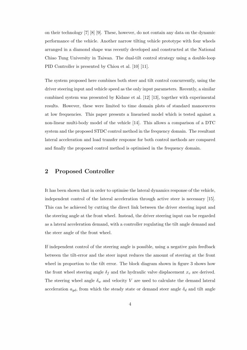
posed controller over the entire frequency range of interest. Figures 22 and 23 show the

lateral acceleration and load transfer response of the original DTC controller (Kδθ =

0) compared to that of the proposed SDTC controller. The system response is shown

for a range of steering gains Kδθ from 0.2 to 0.4. This range was chosen so that the

lateral acceleration amplitude would never exceed the demand lateral acceleration am-

30

10−2

10−1

100

101

−4

−2

0

2

4

frequency (Hz)

ampl

itud

e (d

B)

10−2

10−1

100

101

−100

−50

0

50

frequency (Hz)

phas

e (d

eg)

Figure 20: Bode plot of lateral acceleration response for original controller

10−2

10−1

100

101

30

40

50

60

frequency (Hz)

ampl

itud

e (d

B)

10−2

10−1

100

101

−100

0

100

200

frequency (Hz)

phas

e (d

eg)

Figure 21: Bode plot of load transfer response for original controller

31

plitude. For the previous control method, the actual lateral acceleration can be seen to

exceed the demand lateral acceleration over a significant part of the frequency range,

leading to an increase in the load transfer. This would have been an important factor

contributing to the tendency of the vehicle to roll. With the new control approach

however, the lateral acceleration does not exceed the demand lateral acceleration. As a

result, the load transfer is also reduced over the principal frequency range of 0.1 - 2Hz.

It should be noted that at lower frequencies, the achieved lateral acceleration does not

match the demand lateral acceleration due to the under-steer effect introduced by the

kinematic rear-wheel steer [14]. With the correct amount of rear wheel steer, this would

be much closer to 1 (0dB). In this case a higher steering gain Kδθ would be required to

keep the ratioayayd

as close as possible to 0dB over the principal frequency range. It can

be argued that for a neutral and predictable handling response, the lateral acceleration

response should remain constant across the frequency range. This can be achieved with

a steering gain value of 0.4. By increasing the gain any further, the lateral acceleration

response deviates further from the demand acceleration. Increasing the gain up to 0.4

also leads to a positive effect on the load transfer as can be seen in figure 23. The

system response will be investigated in the time domain to confirm these findings.

7 Time Domain Response

The controller was tuned in the frequency domain with the system linearised about

the centre position and a vehicle forward speed of 30 km/h. Performance will be

investigated in the time domain with the non-linear model. As the principal aim

of the controller is to improve transient performance, a number of manoeuvres will

be investigated where the original control method would have brought the vehicle to

the brink of roll-over (i.e. zero inner wheel load) and the vehicle dynamics of the

original and new control approach are compared. A figure of eight manoeuvre requiring

approximately 1.2kJ of energy from the actuators has been undertaken with the new

control approach using the full non-linear simulation and the lateral acceleration and

load transfer response is compared with the original response in figures 24 and 25.

32

10−2

10−1

100

101

−20

−15

−10

−5

0

5

frequency (Hz)

ampl

itud

e (d

B)

10−2

10−1

100

101

−200

−150

−100

−50

0

50

frequency (Hz)

phas

e (d

eg)

Kδ θ = 0

Kδ θ = 0.2

Kδ θ = 0.3

Kδ θ = 0.4

Figure 22: Bode diagram ofayayd

for original DTC (Kδθ = 0) and new SDTC controller

10−2

10−1

100

101

30

40

50

60

frequency (Hz)

ampl

itud

e (d

B)

10−2

10−1

100

101

−100

0

100

200

frequency (Hz)

phas

e (d

eg)

Kδ θ = 0

Kδ θ = 0.2

Kδ θ = 0.3

Kδ θ = 0.4

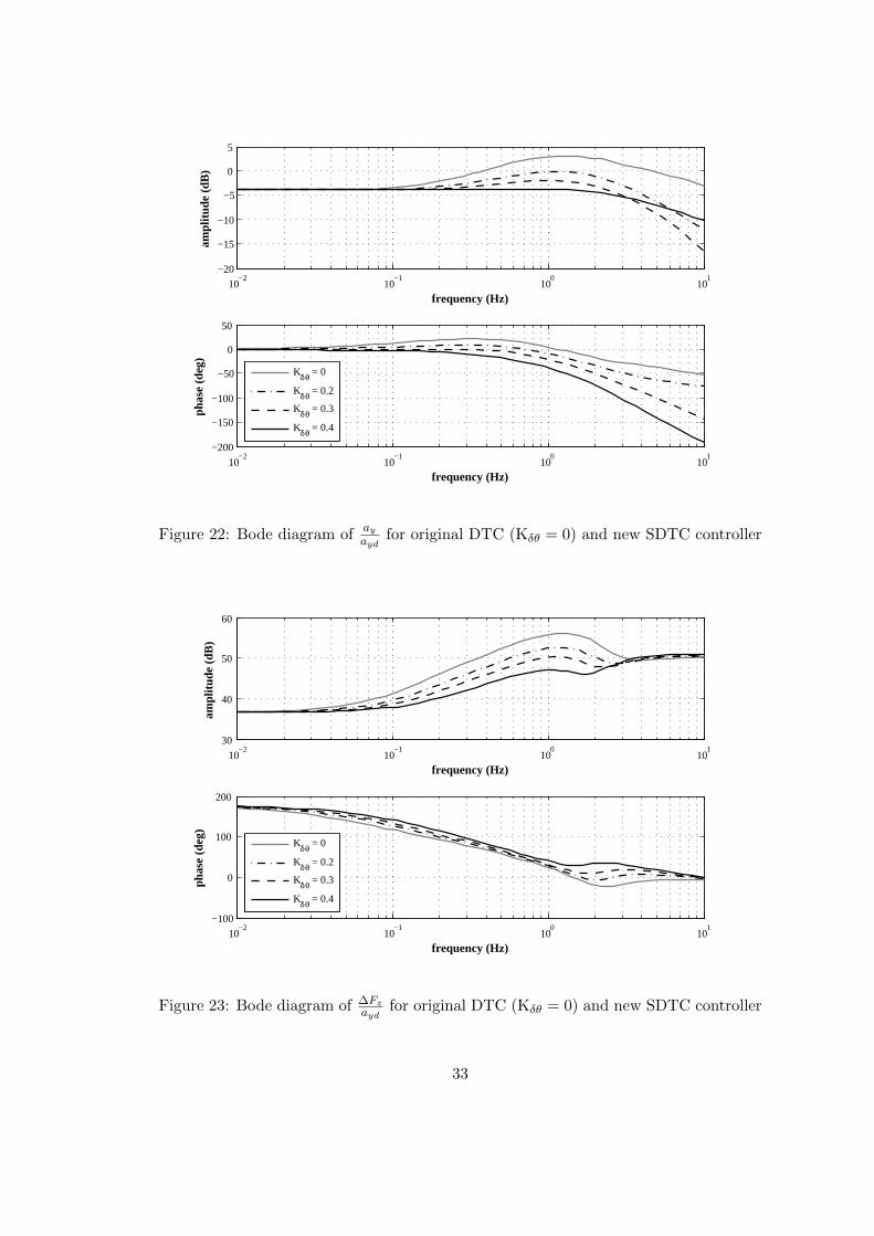
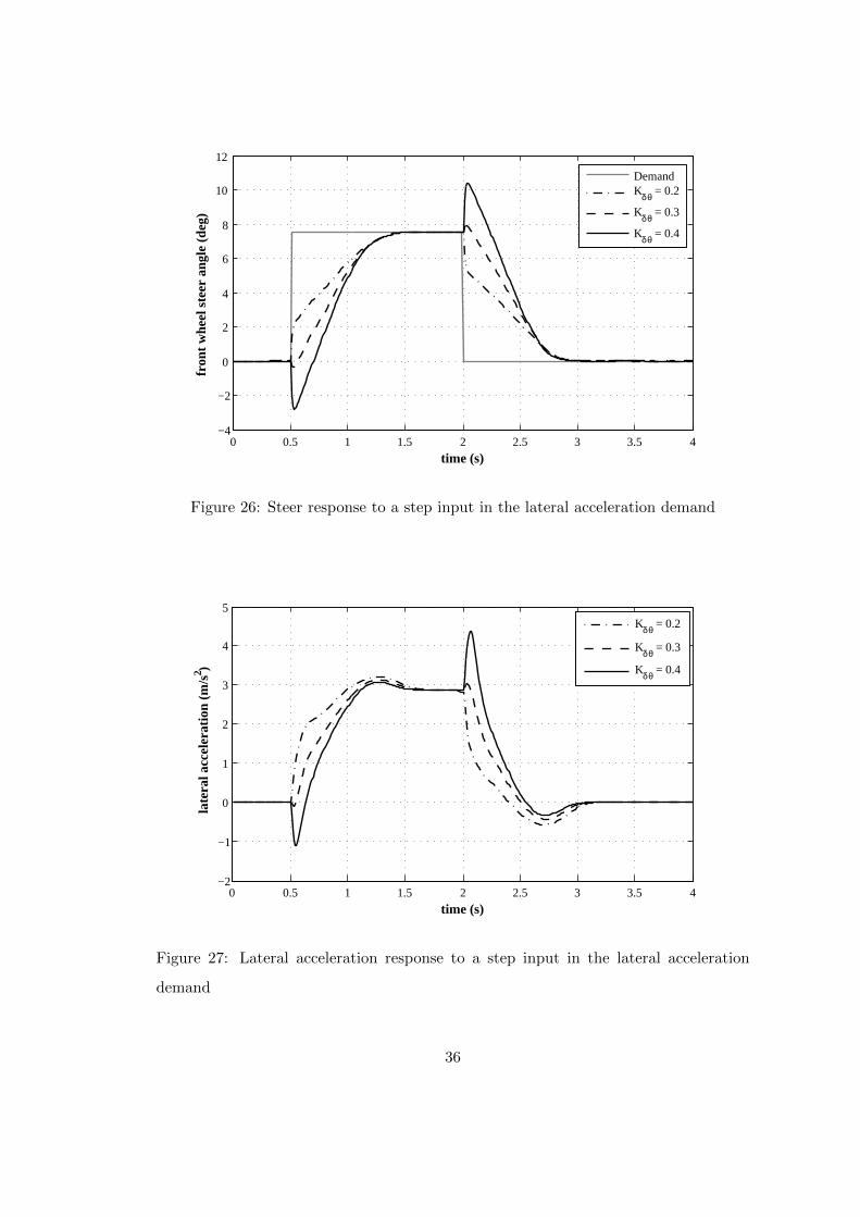
Figure 23: Bode diagram of ∆Fzayd

for original DTC (Kδθ = 0) and new SDTC controller

33

0 1 2 3 4 5 6 7 8−4

−3

−2

−1

0

1

2

3

time (s)

late

ral a

ccel

erat

ion

(m/s

2 )

Kδ θ = 0

Kδ θ = 0.2

Kδ θ = 0.4

Figure 24: Lateral acceleration response for entering and exiting a steady state corner

using the original DTC (Kδθ = 0) and new SDTC controller

0 1 2 3 4 5 6 7 80

500

1000

1500

2000

2500

time (s)

left

whe

el lo

ad (

N)

Kδ θ = 0

Kδ θ = 0.2

Kδ θ = 0.4

Figure 25: Left wheel load for entering and exiting a steady state corner using the

original DTC (Kδθ = 0) and new SDTC controller

34

Looking at figure 24, it can be seen that the lateral acceleration builds up more grad-

ually with the new SDTC control approach. As a result, there is significantly less

over-shoot and the lateral acceleration settles to the steady state value more rapidly.

The more gradual build-up of lateral acceleration and reduced actuator loads lead to

a significant reduction in the load transfer, as shown in figure 25. Whereas with the

previous controller, this manoeuvre would almost lead to the vehicle rolling over, with

the new strategy, the inner wheel load is still in a safe range.

The robustness of the new control method and the effect of the gain Kδθ can be investi-

gated further by looking at the response to a step input requiring approximately 1.3kJ

of energy from the actuators, which may have lead to the vehicle rolling over with the

original control method. Looking at figure 26, it can be seen that increasing the gain

results in some counter-steering. This results in an even smaller load transfer as can

be seen in figure 28 and a faster response in the tilt angle as seen in figure 29. Further-

more, it has the positive effect of reducing over-shoot in the lateral acceleration and

the lateral acceleration settles into steady state more rapidly. It could be argued that

introducing some counter-steer would cause the vehicle to briefly travel in the opposite

direction to that desired. However, with this control strategy, counter-steer would only

occur in extreme situations, where it would be necessary to prevent roll-over. Further-

more, this would only occur for a fraction of a second, and would be unlikely to be

noticed by the driver, similar to the counter-steering effects on a motorcycle. Looking

at the lateral acceleration profile in figure 27, it can be seen that the proportion of

time spent at a negative lateral acceleration is extremely small, but that the benefits

in terms of load transfer are significant. A good value for the steering gain Kδθ at a

driving speed of 30 km/h is confirmed to be 0.4.

The extended stability of the new controller with a steering gain Kδθ of 0.4 can be

shown by a severe manoeuvre requiring 2.3kJ of energy that brings the vehicle to the

brink of roll-over. This is shown in figures 30 and 31. At lateral accelerations of around

8m/s2 the vehicle reaches the adhesion limit of the tyres where the dynamics become

highly non-linear. At this point the inner wheel load almost reaches zero. However,

it can be seen that there is very little additional load transfer as the vehicle tilts back

35

0 0.5 1 1.5 2 2.5 3 3.5 4−4

−2

0

2

4

6

8

10

12

time (s)

fron

t w

heel

ste

er a

ngle

(de

g)

DemandKδ θ = 0.2

Kδ θ = 0.3

Kδ θ = 0.4

Figure 26: Steer response to a step input in the lateral acceleration demand

0 0.5 1 1.5 2 2.5 3 3.5 4−2

−1

0

1

2

3

4

5

time (s)

late

ral a

ccel

erat

ion

(m/s

2 )

Kδ θ = 0.2

Kδ θ = 0.3

Kδ θ = 0.4

Figure 27: Lateral acceleration response to a step input in the lateral acceleration

demand

36

0 0.5 1 1.5 2 2.5 3 3.5 4600

800

1000

1200

1400

1600

1800

2000

2200

time (s)

left

whe

el lo

ad (

N)

Kδ θ = 0.2

Kδ θ = 0.3

Kδ θ = 0.4

Figure 28: Left wheel load response to a step input in the lateral acceleration demand

0 0.5 1 1.5 2 2.5 3 3.5 4−5

0

5

10

15

20

25

30

time (s)

tilt

ang

le (

deg)

Kδ θ = 0.2

Kδ θ = 0.3

Kδ θ = 0.4

Figure 29: Tilt angle response to a step input in the lateral acceleration demand

37

to the original position. The new controller therefore allows the vehicle to be driven

much closer to its physical limits.

The optimal steering gain is velocity dependent. The process was therefore repeated at

10km/h intervals up to 120km/h, which represents the operating range of the vehicle.

The results are shown in figure 32. The optimal value was chosen as the minimum

value of Kδθ that resulted in no increase in theayayd

amplitude profile, similar to that

obtained for Kδθ = 0.4 at 30km/h. With the correct kinematic set-up, this should

result in the lateral acceleration matching the lateral acceleration demand across the

principal frequency range and give a safe and predictable handling performance.

It can be seen that the steering gain reaches horizontal asymptotes at each end of the

speed range. At low speed there is very little lateral force resulting from a steer input

and therefore steering gain has little effect. At high speed, the resultant forces are

much larger and hence a smaller gain is required to achieve the desired response. The

results shown in figure 32 could be applied as a look-up table in the vehicle controller.

8 Concluding Remarks

This paper presents a tilt control concept for a narrow track vehicle, and includes

controller analysis and simulation results using both non-linear and linearised models.

The linear model was shown to give a good fit to the non-linear model. The frequency

domain response of an earlier DTC control system displayed a peak in the lateral

acceleration and load transfer response between 1Hz and 2Hz, which matched the

observations made previously in subjective tests. Around this frequency, the lateral

acceleration was considerably higher than the demand lateral acceleration, as the initial

steering input would lead to large slip angles at the front and rear. This leads to a

large load transfer across the rear axle and is a significant factor contributing to the

potential roll-over of the vehicle.

The proposed control system treats the driver steering input as a lateral acceleration

38

0 0.5 1 1.5 2 2.5 3 3.5 4−4

−2

0

2

4

6

8

10

12

14

16

18

stee

r an

gle

(deg

)

Steer angle

0 0.5 1 1.5 2 2.5 3 3.5 4−2

−1

0

1

2

3

4

5

6

7

8

9

time (s)

late

ral a

ccel

erat

ion

(m/s

2 )

Lateral acceleration

Figure 30: Steer and lateral acceleration response for a severe manoevre

0 0.5 1 1.5 2 2.5 3 3.5 4−10

−2.5

5

12.5

20

27.5

35

42.5

50

tilt

ang

le (

deg)

Tilt angle

0 0.5 1 1.5 2 2.5 3 3.5 40

200

400

600

800

1000

1200

1400

1600

time (s)

inne

r w

heel

load

(N

)

Inner wheel load

Figure 31: Tilt angle and inner wheel load response for a severe manoevre

39

0 20 40 60 80 100 1200.05

0.1

0.15

0.2

0.25

0.3

0.35

0.4

0.45

speed km/h

Kδ θ

Figure 32: Steering gain against forward speed

demand that is to be reached as rapidly as possible and with minimum load transfer

across the rear axle. It utilises a negative gain feedback between the tilt-error and the

steer input, reducing the steering angle as the tilt error increases. As a result the forces

which act on the actuator are significantly reduced and the desired tilt angle can be

reached more rapidly and with less load transfer. The system model was linearised

about the central position at a driving speed of 30km/h, and an ideal steering gain

was determined from the model at this speed. The process was repeated in 10km/h

intervals from 0 - 120km/h to obtain the steering gain over the speed range of the

vehicle.

The frequency response analysis of the proposed SDTC control system indicated a

much more predictable handling response than the original DTC controller, coupled

with reduced load transfer across the rear axle. Using the non-linear model, the lat-

eral acceleration response has less overshoot and the lateral acceleration settles to the

steady state value more rapidly. The resultant rear axle load transfer for a demanding

manoeuvre using the new control method was shown to be approximately 15% of the

original value. The new control method was also shown to result in some counter-

40

steering in rapid steering manoeuvres. This helps to tilt the cabin to the desired tilt

angle and simultaneously reduce load transfer. As a result the controller is shown to be

very robust, even in extreme manoeuvres. Currently work is underway to implement

the controller on the CLEVER vehicle.

41

List of Figures

1 CLEVER test vehicle at the University of Bath . . . . . . . . . . . . . . 2

2 Lifting of inner wheel due to an aggressive steering manoeuvre . . . . . 3

3 Block diagram for proposed control system . . . . . . . . . . . . . . . . 5

4 Schematic diagram showing individual blocks required for the linearisa-

tion of the vehicle system . . . . . . . . . . . . . . . . . . . . . . . . . . 6

5 Bicycle model . . . . . . . . . . . . . . . . . . . . . . . . . . . . . . . . . 8

6 Free body diagram of cabin and rear module viewed from the rear . . . 10

7 Vehicle roll axis before and after a rotation of the cabin about the tilt

axis when keeping the rear module fixed . . . . . . . . . . . . . . . . . . 12

8 Representation of the valve and actuator system . . . . . . . . . . . . . 15

9 Forces acting upon a double ended actuator . . . . . . . . . . . . . . . . 17

10 Linearised block diagram of hydraulic system [6] . . . . . . . . . . . . . 18

11 Controller including position feedback control of the hydraulic system . 19

12 Non-linear tilt angle response and first order linear fit . . . . . . . . . . 20

13 Vehicle multi-body model visualisation . . . . . . . . . . . . . . . . . . . 24

14 Linear and non-linear lateral acceleration response to a steer input . . . 29

15 Linear and non-linear load transfer response to a steer input . . . . . . . 29

16 Linear and non-linear lateral acceleration response to a tilt demand input 29

42

17 Linear and non-linear load transfer response to a tilt demand input . . . 29

18 Linear and non-linear lateral acceleration response to a combined steer

and tilt demand input . . . . . . . . . . . . . . . . . . . . . . . . . . . . 30

19 Linear and non-linear load transfer response to a combined steer and tilt

demand input . . . . . . . . . . . . . . . . . . . . . . . . . . . . . . . . . 30

20 Bode plot of lateral acceleration response for original controller . . . . . 31

21 Bode plot of load transfer response for original controller . . . . . . . . . 31

22 Bode diagram ofayayd

for original DTC (Kδθ = 0) and new SDTC controller 33

23 Bode diagram of ∆Fzayd

for original DTC (Kδθ = 0) and new SDTC controller 33

24 Lateral acceleration response for entering and exiting a steady state cor-

ner using the original DTC (Kδθ = 0) and new SDTC controller . . . . . 34

25 Left wheel load for entering and exiting a steady state corner using the

original DTC (Kδθ = 0) and new SDTC controller . . . . . . . . . . . . 34

26 Steer response to a step input in the lateral acceleration demand . . . . 36

27 Lateral acceleration response to a step input in the lateral acceleration

demand . . . . . . . . . . . . . . . . . . . . . . . . . . . . . . . . . . . . 36

28 Left wheel load response to a step input in the lateral acceleration demand 37

29 Tilt angle response to a step input in the lateral acceleration demand . 37

30 Steer and lateral acceleration response for a severe manoevre . . . . . . 39

31 Tilt angle and inner wheel load response for a severe manoevre . . . . . 39

32 Steering gain against forward speed . . . . . . . . . . . . . . . . . . . . . 40

43

Nomenclature

Ap actuator piston area

a londitudinal distance of front axle to vehicle CoG

ac longitudinal distance of cabin CoG to front axle

ay lateral acceleration

ayd maximum lateral acceleration

aθ longitudinal distance of tilt bearing to front axle

Bp actuator damping coefficient

b longitudinal distance of rear axle to vehicle CoG

bθ actuator tilt/displacement ratio

Ce valve coefficient

Cs suspension damping coefficient

Cαf front tyre slip stiffness coefficient

Cαr rear tyre slip stiffness coefficient

Cθf front tyre camber coefficient

Fl external load on actuators

Fy lateral force on tyre

Fz vertical force on tyre

g gravitational acceleration

hc distance of cabin CoG from ground

hr distance of rear module CoG from ground

hθ distance of tilt bearing from ground

Ic cabin roll inertia about CoG

Ir rear module roll inertia about CoG

Iz vehicle yaw inertia about CoG

Kayd lateral acceleration demand gain

Kδd steer angle demand gain

Kδr rear steer coefficient

Kc pressure gain

Kq flow gain

44

Krφ roll bar stiffness

Ks suspension spring stiffness

Kxv spool displacement gain

Kδθ controller steering gain

Kθd tilt angle demand gain

l distance of tilt bearing to front tyre contact patch

lc see figure 7

L wheel base

m total vehicle mass

mc cabin mass

mr rear module mass

Mt actuator piston mass

Mx moment acting at the tilt bearing

qc flow into actuator due to oil compressibility

Q actuator flow

QL flow through the valve

R corner radius

Rw ratio of steering wheel to front wheel

Ry lateral reaction force at tilt bearing

Rz vertical reaction force at tilt bearing

r yaw rate

T rear wheel track

v lateral velocity component

V vehicle velocity

V fluid volume in single actuator

Vt total fluid volume in hydraulic system

xp actuator piston displacement

xv valve spool displacement

αf front tyre slip angle

αr rear tyre slip angle

45

α′ transient state slip angle

β bulk modulus of hydraulic fluid

βe effective bulk modulus of hydraulic system

δ resultant steer angle

δd demand steer angle at the front wheel

δf front steer angle

δw driver steering angle input at the steering wheel

∆Fz load transfer across rear axle

∆PL load pressure

γ camber angle

µ road surface friction coefficient

φ roll angle of rear module

ψ yaw angle

σ tyre relaxation length

θ relative tilt angle between cabin and rear module

θd demand tilt angle

θss steady state tilt angle of cabin

ω rotational speed

ξ tilt axis inclination

46

References

[1] Anon. “Regulation (EC) No 443/2009 of the European Parliament and of the

Council of 23 April 2009 setting emission performance standards for new passenger

cars as part of the Community’s integrated approach to reduce CO 2 emissions

from light-duty vehicles (Text with EEA relevance)”. Technical report, European

Parliament, Council, 2009. Procedure number: COD(2007)0297.

[2] S-G. So and D. Karnopp. “Switching strategies for narrow ground vehicles with

dual mode automatic tilt control”. Int. J. of Vehicle Design, 18(5):518–532, 1997.

[3] S. So and D. Karnopp. “Active Dual Mode Tilt Control for Narrow Ground

Vehicles”. Vehicle System Dynamics, 27:19–36, 1997.

[4] D. Karnopp. “The Dynamics of Narrow, Automatically Tilted Commuter Vehi-

cles”. In Proceedings of the 1997 EAEC Congress: Lightweight and small cars:

the answer to future needs, pages 13–19, 1997. Paper number 97A2KN08.

[5] B. Drew. “Tilt Control for a Narrow Track Vehicle”. Obtained from:

http://www.bath.ac.uk/ptmc/research/docs/ proj_tilting_vehicle.pdf.

[6] B. Drew. Development of Active Tilt Control For A Three-Wheeled Vehicle. PhD

thesis, University of Bath, Bath, UK, 2006.

[7] C. van den Brink and H. Kroonen. “Dynamic Vehicle Control for Enclosed Narrow

Vehicles”. In Proceedings of EAEC 6th European Congress: Lightweight and Small

Cars—The Answer to Future Needs, 2–4 July 1997. Paper number 97A2I22.

[8] C Van den Brink and H. Kroonen. “DVC — The banking technology driving the

CARVER vehicle class”. In Proceedings of the 7th International Symposium on

Advanced Vehicle Control (AVEC04), 13–20 Aug 2004.

[9] C. van den Brink and H. Kroonen. “Slender Comfort Vehicles: Offering the Best

of Both Worlds”. AutoTechnology, pages 56–59, 1/2004.

47

[10] J. C. Chiou and C. L. Chen. “Modeling and Verification of a Diamond-Shape

Narrow-Tilting Vehicle”. IEEE/ASME Transactions on Mechatronics, 13(6):678–

691, 2008.

[11] J. C. Chiou, C. Y. Lin, C. L. Chen, and Chien C. P. “Tilting Motion Control in

Narrow Tilting Vehicle Using Double-Loop PID Controller”. In Proceedings of the

7th Asian Control Conference, pages 913–918, Hong Kong, China, 27–29 August

2009.

[12] S. Kidane, R. Rajamani, L. Alexander, P. Starr, and M. Donath. “Development

and Experimental Evaluation of a Tilt Stability Control System for Narrow Com-

muter Vehicles”. In IEEE Transactions on Control Systems Technology, volume 18,

Nov 2010.

[13] S. Kidane, L. Alexander, R. Rajamani, P. Starr, and M. Donath. “A fundamen-

tal investigation of tilt control systems for commuter vehicles”. Vehicle System

Dynamics, 46(4):295–322, 2008.

[14] J. Berote. Dynamics and Control of a Tilting Three Wheeled Vehicle. PhD thesis,

University of Bath, Bath, UK, 2010.

[15] J. Berote, A. Plummer, and J Darling. “Lateral Dynamics Optimisation of a

Direct Tilt Controlled Narrow Vehicle”. In Proceedings of the 10th International

Symposium on Advanced Vehicle Control (AVEC 2010), 22–26 Aug 2010.

[16] M. Barker, B. Drew, J. Darling, K. Edge, and G. W. Owen. “Steady-State Steering

of a Tilting Three-Wheeled vehicle”. Vehicle System Dynamics, 48(7):815–830,

2010.

[17] V. Cossalter. “Motorcycle Dynamics 2nd Edition”. LuLu (Self Publishing), 2006.

[18] H. B. Pacejka. “Tyre and Vehicle Dynamics”. Butterworth-Heinemann, 2002.

[19] H. S. Radt and W.F. Milliken. “Non-dimensionalizing Tyre Data for Vehicle Sim-

ulation”. Road Vehicle Handling, 1983.

[20] W. F. Milliken and D. L. Milliken. “Race Car Vehicle Dynamics”. SAE, 1995.

48