AC 2010-1011: DEVELOPMENT OF A SAMPLE TUTORIAL FOR METALFORMING USING ADVANCED COMPUTER AIDED ENGINEERING TOOLS

Raghu Echempati, Kettering University

Andy Fox, Kettering University

© American Society for Engineering Education, 2010

Page 15.407.1

A SAMPLE TUTORIAL FOR SHEET METAL FORMING ANALYSIS

USING ADVANCED COMPUTER AIDED ENGINEERING TOOLS

Abstract

In this paper, a sample tutorial has been developed using advanced CAE tools like HyperWorks

and LS-Dyna. The work outlined in this paper is routinely carried by experienced engineers in an

industry environment. However, it is believed that the tutorial presented here is believed to be

unique in an educational setup. Although many CAE software offer online tutorials relevant to

the use of that specific software, there are very few if any that offer help sheets that require a

user to switch between different software for carrying out the numerical simulations. A senior

level course on metal forming simulation requires the use of various CAE tools to do solid

modeling and to carry out the finite element modeling and analysis.

An assessment to measure the effectiveness of the use of this tutorial is yet to be fully developed,

but it appears based on preliminary survey that the students seem to have appreciated the ease

with which the simulations can be carried out based on this tutorial. Also due to an increased

demand for trained engineers in the metal forming area such tutorials are very helpful as a first

step. A step by step procedure has been written that integrates the use of different CAE tools for

metal forming simulation of an example instrument panel (IP) used in automotive applications.

As a first step, solid modeling of the individual sheet metal component using different CAD

programs like Unigraphics is discussed. A discussion on how these solid models can be imported

to different CAE programs to be meshed and then subsequently used in high-end solvers like

HyperForm and LSDyna is then presented.

The analyses that were conducted for this tutorial included formability of the individual

component. Design of Experiments used in this study is also briefly discussed. The main purpose

of doing these types of analyses is to choose the optimum design based on the set constraints.

The DOE studies presented in this paper can be adapted in an educational environment. DOE

was done to determine the effects that the input factors have on the results of the forming

simulations that were conducted. This integrated study can be used in a senior manufacturing

simulation course. Finally, the results of this study are discussed and recommendations for future

work presented.

Introduction

In this paper, a sample tutorial for a metal forming simulation using HyperForm (one-step

solver) of HyperWorks is presented and discussed. Other tutorials based on using the large

deformation nonlinear finite element code – LS-Dyna (incremental solver) has also been

developed. The results from both of these software programs are compared for consistency and

validation purposes. Due to space limitations only a sample tutorial based on HyperForm is

presented below. Students’ feedback indicates that the developed tutorial is very useful for their

easy understanding of both meshing and analysis of large deformation metal stamping analysis.

Page 15.407.2

Modeling, Meshing, and Simulating a Bracket Used in an Instrument Panel using

(UGS NX 5.0 / HyperMesh 9.0 / HyperForm 9.0)1,2

This tutorial creates and analyzes a sheet metal stamped part that is used to hold a steering

column onto an instrument panel shown below. A solid model of the part is created using UGS

NX 5.0 and then is meshed using HyperMesh 9.0. A stamping simulation is then performed

using HyperForm. A DOE is conducted on the results of the simulation and a brief description is

provided.

Figure 1 – Component used in the analysis

Solid Modeling

1. Open NX 5.0 - Open the CAD program NX

5.0 by going to the Start button in the lower

left corner of the screen then All Programs

then UGS NX 5.0 then NX 5.0

2. Create a .prt File - Go to File then New

then in the File New window that pops up

make sure Model is highlighted under the

Templates section and then in the New File

Name section name it something and save it

somewhere you will remember and then

click OK.

Figure 2 – Name and save the model file using this window

Page 15.407.3

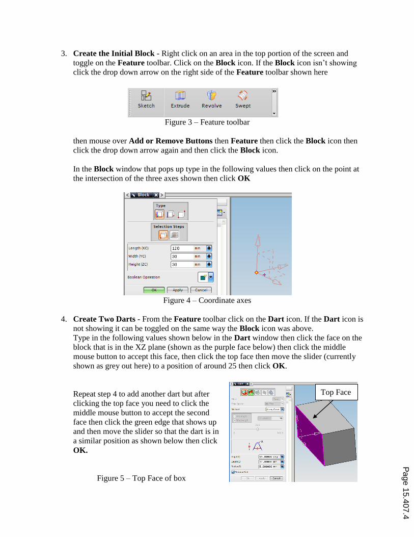
3. Create the Initial Block - Right click on an area in the top portion of the screen and

toggle on the Feature toolbar. Click on the Block icon. If the Block icon isn’t showing

click the drop down arrow on the right side of the Feature toolbar shown here

Figure 3 – Feature toolbar

then mouse over Add or Remove Buttons then Feature then click the Block icon then

click the drop down arrow again and then click the Block icon.

In the Block window that pops up type in the following values then click on the point at

the intersection of the three axes shown then click OK

Figure 4 – Coordinate axes

4. Create Two Darts - From the Feature toolbar click on the Dart icon. If the Dart icon is

not showing it can be toggled on the same way the Block icon was above.

Type in the following values shown below in the Dart window then click the face on the

block that is in the XZ plane (shown as the purple face below) then click the middle

mouse button to accept this face, then click the top face then move the slider (currently

shown as grey out here) to a position of around 25 then click OK.

Repeat step 4 to add another dart but after

clicking the top face you need to click the

middle mouse button to accept the second

face then click the green edge that shows up

and then move the slider so that the dart is in

a similar position as shown below then click

OK.

Figure 5 – Top Face of box

Top Face

Page 15.407.4

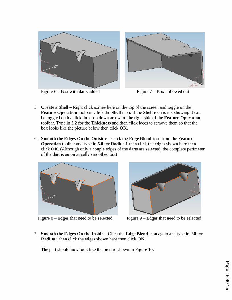
Figure 6 – Box with darts added Figure 7 – Box hollowed out

5. Create a Shell – Right click somewhere on the top of the screen and toggle on the

Feature Operation toolbar. Click the Shell icon. If the Shell icon is not showing it can

be toggled on by click the drop down arrow on the right side of the Feature Operation

toolbar. Type in 2.2 for the Thickness and then click faces to remove them so that the

box looks like the picture below then click OK.

6. Smooth the Edges On the Outside – Click the Edge Blend icon from the Feature

Operation toolbar and type in 5.0 for Radius 1 then click the edges shown here then

click OK. (Although only a couple edges of the darts are selected, the complete perimeter

of the dart is automatically smoothed out)

Figure 8 – Edges that need to be selected Figure 9 – Edges that need to be selected

7. Smooth the Edges On the Inside – Click the Edge Blend icon again and type in 2.8 for

Radius 1 then click the edges shown here then click OK.

The part should now look like the picture shown in Figure 10.

Page 15.407.5

Figure 10 – Correct shape of part

8. Create Two Holes – Go to Insert then Design Feature then Hole. Enter 10 for the

Diameter then click the top surface of the part then click the bottom surface of the part to

specify the thru face and then click Apply.

Figure 11 – Surface to create holes in Figure 12 – First edge used to place the hole

Then click the edge shown below and then type 30 in the box shown then click Apply.

Then click the top edge shown then type in 20 in the box shown then click OK.

Page 15.407.6

Figure 13 – Second edge used to place the hole Figure 14 – Current shape of the component

Repeat the same process to create another hole that has a distance of 90 from the first edge

and 20 from the second edge so that the part looks like the following picture.

9. Remove Lower Edge – Go to Insert then Sketch then click the face shown below then

click OK.

Figure 15 – Face used to create the sketch

Go to Insert then Rectangle to create a rectangle that is approximately the same size as

shown. Make sure the right side and bottom of the rectangle are outside of the part as

shown. Then click the Finish Sketch icon.

Go to Insert then Design Feature then

Extrude then click the sketch that was just

created. Then drag the ends of the arrow

that appears so that the ends of the see thru

box are outside of the part as shown and

then click OK.

Figure 16 – The sketch that is created on the face

Page 15.407.7

Figure 17 – Extruded box

Then go to Insert then Combine Bodies then Subtract then click the original part then click

the solid box that was just created then click OK. The part should now look like the picture

shown below.

Figure 18 – Subtracted corner

The blue sketch can be hidden by hitting the keys ctrl-w and then expanding the Geomtry

tree and then clicking the minus sign next to Sketches.

10. Create Radii at the Edges – Click the Edge Blend icon on the Feature Operation

toolbar and then enter 10 for the Radius 1 value then click the five highlighted edges

shown below then click OK.

Page 15.407.8

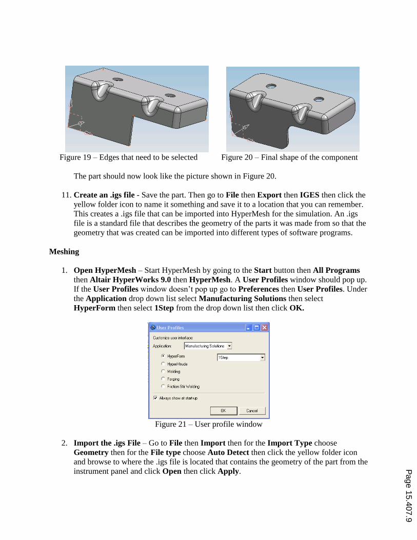
Figure 19 – Edges that need to be selected Figure 20 – Final shape of the component

The part should now look like the picture shown in Figure 20.

11. Create an .igs file - Save the part. Then go to File then Export then IGES then click the

yellow folder icon to name it something and save it to a location that you can remember.

This creates a .igs file that can be imported into HyperMesh for the simulation. An .igs

file is a standard file that describes the geometry of the parts it was made from so that the

geometry that was created can be imported into different types of software programs.

Meshing

1. Open HyperMesh – Start HyperMesh by going to the Start button then All Programs

then Altair HyperWorks 9.0 then HyperMesh. A User Profiles window should pop up.

If the User Profiles window doesn’t pop up go to Preferences then User Profiles. Under

the Application drop down list select Manufacturing Solutions then select

HyperForm then select 1Step from the drop down list then click OK.

Figure 21 – User profile window

2. Import the .igs File – Go to File then Import then for the Import Type choose

Geometry then for the File type choose Auto Detect then click the yellow folder icon

and browse to where the .igs file is located that contains the geometry of the part from the

instrument panel and click Open then click Apply.

Page 15.407.9

3. Shade the Geometry – Click the icon to shade the geometry. By holding down the

ctrl key on the key board and left clicking on the screen and holding down the left mouse

button and moving the mouse around the part can be moved around. To change the origin

of rotation hold down the ctrl key and left click somewhere on the part and let go.

4. Create a Midsurface – Go to

Geometry then AutoCleanup

then click the green edit

parameters box and then the

following window will pop up.

Change the Target element size:

to a value of 6 and then add a

check mark in the box next to

Extract midsurfaces and then

uncheck the box next to Sheet

metal only. Leave everything

else as the default values as

shown below and then click OK.

F

Figure 22 – Midsurface parameters

Click the green edit criteria box then change the Target element size: to a value of 6

then change the Min Size value to 3 and leave everything else as their default values as

shown below and then click OK.

Click the yellow surfs button and then

click all then click autocleanup. The

cleanup should take a few seconds and

then click return. The midsurface

should look similar to the picture

below.

Figure 23 – Mesh parameters

Page 15.407.10

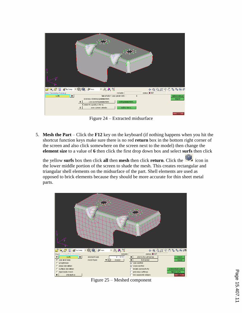
Figure 24 – Extracted midsurface

5. Mesh the Part – Click the F12 key on the keyboard (if nothing happens when you hit the

shortcut function keys make sure there is no red return box in the bottom right corner of

the screen and also click somewhere on the screen next to the model) then change the

element size to a value of 6 then click the first drop down box and select surfs then click

the yellow surfs box then click all then mesh then click return. Click the icon in

the lower middle portion of the screen to shade the mesh. This creates rectangular and

triangular shell elements on the midsurface of the part. Shell elements are used as

opposed to brick elements because they should be more accurate for thin sheet metal

parts.

Figure 25 – Meshed component

Page 15.407.11

6. Turn Off the Geometry – Hit the F5 key on the keyboard (if nothing happens when you

hit the shortcut function keys make sure there is no red return box in the bottom right

corner of the screen and also click somewhere on the screen next to the model) and then

click the drop down box and choose surfs then click the yellow surfs box and then

choose all then click mask.

7. Cleanup the Mesh – Hit the F6 key on the keyboard then click the cleanup button then

select displayed elements from the drop down box then click cleanup.

Figure 26 – Cleanup all displayed elements

Then click the set ranges box and enter the numbers as shown below.

Figure 27 – Cleanup parameters

Check the boxes next to skew and length and leave the other boxes checked. The part should

look similar to what is shown below.

Figure 28 – Red elements that need to

be cleaned up

Page 15.407.12

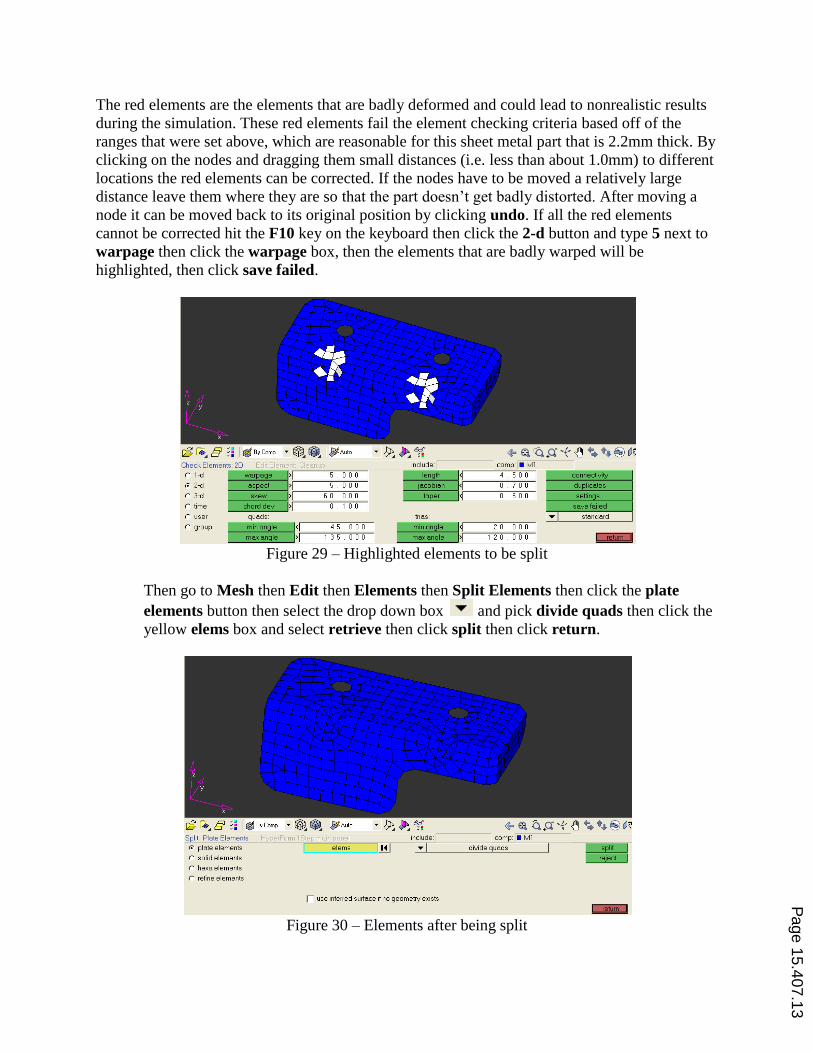
The red elements are the elements that are badly deformed and could lead to nonrealistic results

during the simulation. These red elements fail the element checking criteria based off of the

ranges that were set above, which are reasonable for this sheet metal part that is 2.2mm thick. By

clicking on the nodes and dragging them small distances (i.e. less than about 1.0mm) to different

locations the red elements can be corrected. If the nodes have to be moved a relatively large

distance leave them where they are so that the part doesn’t get badly distorted. After moving a

node it can be moved back to its original position by clicking undo. If all the red elements

cannot be corrected hit the F10 key on the keyboard then click the 2-d button and type 5 next to

warpage then click the warpage box, then the elements that are badly warped will be

highlighted, then click save failed.

Figure 29 – Highlighted elements to be split

Then go to Mesh then Edit then Elements then Split Elements then click the plate

elements button then select the drop down box and pick divide quads then click the

yellow elems box and select retrieve then click split then click return.

Figure 30 – Elements after being split

Page 15.407.13

Try to cleanup the remaining failed elements again by hitting the F6 key. The simulation

will still run if there are failed elements, unless they are severely distorted. Results of the

simulation will be closer to the actual physical results of the stamping process if the

quality of the mesh is good. It should be mentioned that triangular elements tend to

stiffen the part which leads to erroneous results as well, therefore the less triangular

elements the better.

Simulate the Stamping Process

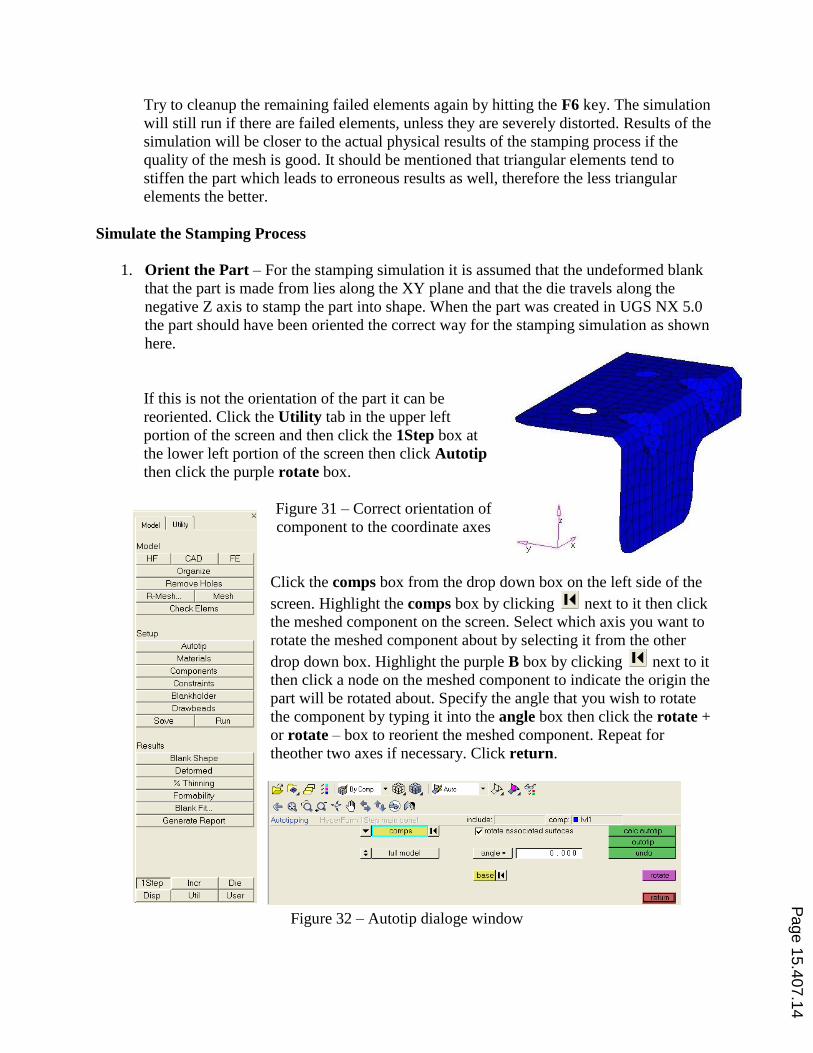
1. Orient the Part – For the stamping simulation it is assumed that the undeformed blank

that the part is made from lies along the XY plane and that the die travels along the

negative Z axis to stamp the part into shape. When the part was created in UGS NX 5.0

the part should have been oriented the correct way for the stamping simulation as shown

here.

If this is not the orientation of the part it can be

reoriented. Click the Utility tab in the upper left

portion of the screen and then click the 1Step box at

the lower left portion of the screen then click Autotip

then click the purple rotate box.

Figure 31 – Correct orientation of

component to the coordinate axes

Click the comps box from the drop down box on the left side of the

screen. Highlight the comps box by clicking next to it then click

the meshed component on the screen. Select which axis you want to

rotate the meshed component about by selecting it from the other

drop down box. Highlight the purple B box by clicking next to it

then click a node on the meshed component to indicate the origin the

part will be rotated about. Specify the angle that you wish to rotate

the component by typing it into the angle box then click the rotate +

or rotate – box to reorient the meshed component. Repeat for

theother two axes if necessary. Click return.

Figure 32 – Autotip dialoge window

Page 15.407.14

Figure 33 – Point where component will be rotated about

Select comps from the drop down box then highlight comps by clicking next to it

then click the meshed component on the screen and then click calc autotip then click

return.

Figure 34 – Autotip dialogue window

You can tell if the part is oriented correctly later when the simulation is ran because if it

isn’t an undercut error will occur and the orientation will need to be adjusted again. The

side of the part that is being undercut will be highlighted when the simulation is ran to

indicate where the error is.

2. Create the Material Collector – On the left side of the screen click Material then click

the create button then rename the material and type in the vales as shown below (which

is for AISI 1008 steel) and then click the create box or update if there is already a

material collector with this name.

Page 15.407.15

Figure 35 – Material parameters

3. Create the Component Collector – Click Components on the left side of the screen

then click the component: box (you may need to click it twice) then click the box with

the name of the component (there should only be one and it may be named different than

lvl1) then click the material box and click the material collector that was created earlier

then type in 2.2 for the thickness then click update. (do not click create since a

component should already exists)

Figure 36 – Component collector dialogue

4. Create Constraints – Click Constraints on the left side of the screen then click two

nodes in the approximate location as shown (the nodes need to be on elements that lie

along the XY plane) then click update.

Figure 37 – Points where the component is constrained

Page 15.407.16

5. Create the Blankholder – Click Blankholder on the left side of the screen then name it

Blank and type in the values as shown below, then click the yellow elems box and then

click on plane then select three nodes on the blank surface (shown in light blue below) to

define the plane that contains the elements to be selected then click create. The

blankholder is used to define the plane that is perpendicular to the path that the punch

travels to create the part.

Figure 38 – Blankholder surface

6. Save and Run the Simulation – Click Save on the left side of the screen then click save

as then save the file as a Hyperform Binary File (*.hf*) to a separate folder called

Simulation someplace you can remember.

Figure 39 – Window used to save the component

Click Run on the left side of the screen and then click run analysis.

Page 15.407.17

Figure 40 – Window used to run the simulation

A DOS window should pop up and after a few seconds should say that the processing is

complete. The simulation is ran in the Simulation folder that was created earlier and all

the results are copied to this folder.

View the Results

1. Load the Results – Go to File then Load then Results then browse to where the

Simulation folder is and open the .res file then click Open.

2. View Thinning – Click % Thinning on the left side of the screen and then the results

should look similar to what is shown below. The results show that the maximum %

thinning is 20% at the corner shown in red. This is usually the value where splits in sheet

metal start to occur (depending on the type of material used) from too much thinning of

the material. If this was an issue the lower edge of the part could be raised which should

lower the % thinning to correct the problem or the initial thickness of the part could be

increased as well. This % thinning is the percentage that the thickness of the sheet metal

will be reduced from its original thickness during the stamping process.

Figure 41 – Thinning results of the component

Page 15.407.18

3. View Formability – Click Formability on the left side of the screen and then the results

should look similar to what is shown below. Formability tells you whether or not the part

that is being analyzed will have any problems during the manufacturing process. There

are no red Failure zones shown on the meshed part and all of the corresponding points

from each element that are plotted on the FLD curve in the upper right corner of the

screen are below the yellow marginal line. This indicates that if the material used to make

the part has properties that are close to the ones that were specified for the analysis then

the part should not see any splits during the manufacturing process. If any points are

plotted above the yellow marginal line it indicates that splits may occur and if they fall

above the red line then splits are predicted to occur and the part should be redesigned.

Figure 42 – Forming limit diagram

Design of Experiments3-5

Since many simulations can be performed on a stamping process to analyze several designs, a

DOE (design of experiments) is used in this paper to determine which factors and interactions

play the most important role in the forming process and hence effect the thinning. The same

stamping simulation is performed while adjusting different factors like friction, material

thickness, and tonnage for each simulation to determine which factors influence the formability

(e.g. % thinning) of the part. One of the easiest DOE’s to perform is the 2k Factorial Design. The

2 represents the two levels (values) that each of the k factors can assume in the experiment. For

this analysis there were originally four (k = 4) factors in the process, the yield strength of the

sheet metal, its thickness, the friction coefficient, and the tonnage of the press. For each complete

trial or replication of the experiment all possible combinations of the levels of the factors are

investigated. The number of runs can grow quickly though if more than four factors want to be

investigated because a 2k factorial requires 2k combinations. With four factors this DOE

required 24 = 16 complete trials. The 2k factorial can be performed easily by setting up a

spreadsheet that uses factor values and the thinning (response) of each complete trial as inputs

and then the results (effects and interactions) are determined by using contrasts5. This can also

easily be done using the regression data analysis tool in Excel. The results of the DOE can be

used to find the optimum settings of the four factors to minimize the percent thinning (the

Page 15.407.19

response) of one of the corners of the part. Table 1 shows the factor values that were used in the

analysis.

Table 1 – Factor level used in the DOE Studies

Factor

Level

Yield

Strength

(Mpa)

Thickness

(mm) Friction

Tonnage

(Tons)

-1 186 0.8 0.05 20

+1 500 3.2 0.70 80

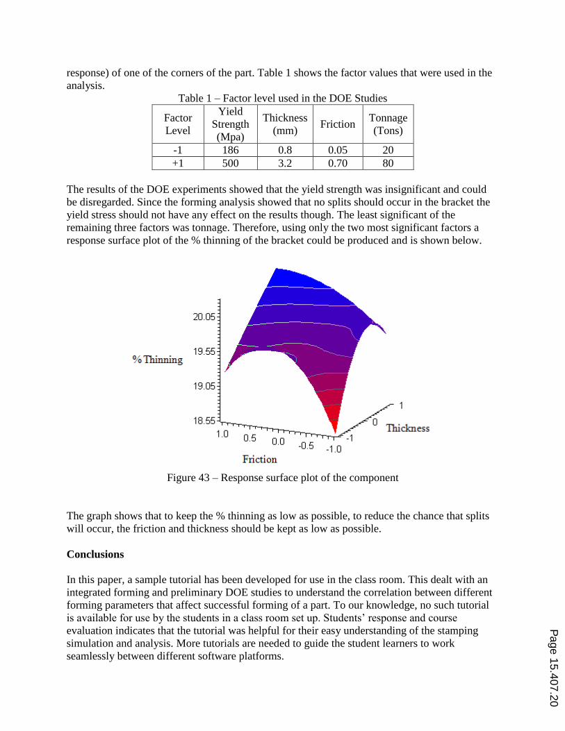
The results of the DOE experiments showed that the yield strength was insignificant and could

be disregarded. Since the forming analysis showed that no splits should occur in the bracket the

yield stress should not have any effect on the results though. The least significant of the

remaining three factors was tonnage. Therefore, using only the two most significant factors a

response surface plot of the % thinning of the bracket could be produced and is shown below.

Figure 43 – Response surface plot of the component

The graph shows that to keep the % thinning as low as possible, to reduce the chance that splits

will occur, the friction and thickness should be kept as low as possible.

Conclusions

In this paper, a sample tutorial has been developed for use in the class room. This dealt with an

integrated forming and preliminary DOE studies to understand the correlation between different

forming parameters that affect successful forming of a part. To our knowledge, no such tutorial

is available for use by the students in a class room set up. Students’ response and course

evaluation indicates that the tutorial was helpful for their easy understanding of the stamping

simulation and analysis. More tutorials are needed to guide the student learners to work

seamlessly between different software platforms.

Page 15.407.20

Bibliography

1. Introduction to UG-NX5 – Cast Tutorials.

2. HyperWorks by Altair Engineering.

3. Moaveni, Seed, “Finite Element Analysis,” 3rd ed., Prentice-Hall, 2008

4. Kreyszig, E., “Advanced Engineering Mathematics’”, J. Wiley. 2006.

5. Jenning, Alan, “Matrix Computation for Engineers and Scientists”, J. Wiley, 1988.

Page 15.407.21