Development of a Minichannel Compact Primary Heat ... · Development of a Minichannel Compact...
133
Development of a Minichannel Compact Primary Heat Exchanger for a Molten Salt Reactor Matthew Stephen Lippy Thesis submitted to the faculty of the Virginia Polytechnic Institute and State University in partial fulfillment of the requirements for the degree of Master of Science In Mechanical Engineering Mark A. Pierson Srinath V. Ekkad Robert W. Hendricks April 28, 2011 Blacksburg, VA Keywords: compact heat exchanger, molten salt reactor, primary heat exchanger
Transcript of Development of a Minichannel Compact Primary Heat ... · Development of a Minichannel Compact...

Development of a Minichannel Compact Primary Heat
Exchanger for a Molten Salt Reactor
Matthew Stephen Lippy
Thesis submitted to the faculty of the Virginia Polytechnic Institute and State University in
partial fulfillment of the requirements for the degree of
Master of Science
In
Mechanical Engineering
Mark A. Pierson
Srinath V. Ekkad
Robert W. Hendricks
April 28, 2011
Blacksburg, VA
Keywords: compact heat exchanger, molten salt reactor, primary heat exchanger

Development of a Compact Primary Heat Exchanger for a
Molten Salt Reactor
Matthew Stephen Lippy
Abstract
The first Molten Salt Reactor (MSR) was designed and tested at Oak Ridge National Laboratory
(ORNL) in the 1960’s, but recent technological advancements now allow for new components,
such as heat exchangers, to be created for the next generation of MSR’s and molten salt-cooled
reactors. The primary (fuel salt-to-secondary salt) heat exchanger (PHX) design is shown here to
make dramatic improvements over traditional shell-and-tube heat exchangers when changed to a
compact heat exchanger design. While this paper focuses on the application of compact heat
exchangers on a Molten Salt Reactor, many of the analyses and results are similarly applicable to
other fluid-to-fluid heat exchangers.
The heat exchanger design in this study seeks to find a middle-ground between shell-and-tube
designs and new ultra-efficient, ultra-compact designs. Complex channel geometries and micro-
scale dimensions in modern compact heat exchangers do not allow routine maintenance to be
performed by standard procedures, so extended surfaces will be omitted and hydraulic diameters
will be kept in the minichannel regime (minimum channel dimension between 200 µm and 3
mm) to allow for high-frequency eddy current inspection methods to be developed. High aspect
ratio rectangular channel cross-sections are used. Various plant layouts of smaller heat exchanger
banks in a “modular” design are introduced.
FLUENT was used within ANSYS Workbench to find optimized heat transfer and
hydrodynamic performance. With similar boundary conditions to ORNL’s Molten Salt Breeder
Reactor’s shell-and-tube design, the compact heat exchanger interest in this thesis will lessen
volume requirements, lower fuel salt volume, and decrease material usage.

iii
Acknowledgements
I have to first thank my family for giving me the opportunity to come to Virginia Tech and
pursue my degrees. I also have to thank my girlfriend, Kristin, who was a tremendous help
throughout Graduate School. Without the love and support from Kristin and my family, the last
two years would have been impossible.
I would like to thank the three members of my committee for their help throughout my research.
Dr Pierson’s guidance was much appreciated throughout my Master’s, and I would not have had
the opportunity to pursue this degree without his help. Dr Ekkad and Dr. Hendricks were also
very important in providing insight throughout my research.
I would also like to thank Debamoy Sen for his constant help with FLUENT and the CFD design
process. Much of the progress made in the research resulted from Debamoy’s guidance in
performing sound and meaningful CFD simulations.

iv
Table of Contents Abstract ..................................................................................................................................... ii
Acknowledgements ................................................................................................................... iii
Table of Figures ....................................................................................................................... vii
I. Introduction .............................................................................................................................1
Current Energy Supply and Demand ........................................................................................1
Nuclear Power for the Future ...................................................................................................2
Thorium as a Nuclear Fuel .......................................................................................................4
Molten Salt Reactors ...............................................................................................................8
Primary Heat Exchanger ........................................................................................................ 14
Compact Heat Exchangers ..................................................................................................... 15
Compact Heat Exchanger History ...................................................................................... 16
Compact Heat Exchangers in a MSR .................................................................................. 18
Heat Exchanger Design ......................................................................................................... 18
II. Literature Review ................................................................................................................. 20
Compact Heat Exchanger Basics ........................................................................................... 20
Related ORNL Studies .......................................................................................................... 24
Compact Heat Exchanger Developments ............................................................................... 31
Nuclear-related Compact Heat Exchanger Research .............................................................. 34
III. Design and Setup................................................................................................................. 40
Design Considerations ........................................................................................................... 40
Maintenance and Inspection ............................................................................................... 41
Corrosion ........................................................................................................................... 43
Plant Layout ....................................................................................................................... 43
Manufacturing.................................................................................................................... 47
Materials ............................................................................................................................ 49
Heat Exchanger Design ......................................................................................................... 51
Design Changes ................................................................................................................. 51
Assumptions .......................................................................................................................... 55
Symmetry .......................................................................................................................... 55
Perfect Casting ................................................................................................................... 57
v
Corrosion/Erosion Effects Negligible ................................................................................. 57
Steady-state Operation ....................................................................................................... 57
Single-Phase Flow ............................................................................................................. 58
Outer Wall of Heat Exchanger Boundary Condition ........................................................... 58
Roughness Effects .............................................................................................................. 58
Inlet/Outlet Effects ............................................................................................................. 58
Composition-dependent Salt Properties .............................................................................. 59
Temperature-dependent Salt Properties .............................................................................. 62
FLUENT Design Process ....................................................................................................... 64
Geometry ........................................................................................................................... 64
Mesh .................................................................................................................................. 67
FLUENT Setup .................................................................................................................. 70
Solution ............................................................................................................................. 72
Results ............................................................................................................................... 73
Parameter Set ..................................................................................................................... 76
Optimization .......................................................................................................................... 82
Design of Experiments (DOE)............................................................................................ 82
Optimization ...................................................................................................................... 83
Results and Discussion .......................................................................................................... 84
Model Validation Theory ................................................................................................... 84
Model Validation Results ................................................................................................... 93
Comparison of Circular and Slotted Designs ...................................................................... 95
Full-Scale ........................................................................................................................... 98
IV. Conclusions and Recommendations .................................................................................. 103
References .............................................................................................................................. 105
Appendix A: ORNL Plant Diagrams ....................................................................................... 109
Appendix B: Parametric Mesh Study ....................................................................................... 110
Preliminary Mesh Study ...................................................................................................... 110
Full-scale Mesh Study ......................................................................................................... 111
Appendix C: Preliminary Study Geometry Calculations .......................................................... 113
Appendix D: ORNL Shell-and-tube Calculations .................................................................... 114

vi
Surface Area Calculation ..................................................................................................... 114
Volume Calculation ............................................................................................................. 114
Material Calculation ............................................................................................................ 114
Output Parameter Calculation .............................................................................................. 115
Appendix E: Material Properties ............................................................................................. 116
Hastelloy N ......................................................................................................................... 116
Composition (weight %) (Haynes International, 2002) ..................................................... 116
Average Physical Properties ............................................................................................. 116
Fuel Salt .............................................................................................................................. 117
Coolant Salt ......................................................................................................................... 118
Appendix F: Laminar-Turbulent Transition Discussion ........................................................... 119
Appendix G: Velocity and Temperature Contours ................................................................... 120
Temperature profile at half channel width along length of channel ....................................... 120
Temperature profiles at varying distances along channel length ........................................... 121
Figure 58: Temperature profile at half channel length, with Symmetry planes mirrored ....... 123
Appendix H: Slotted HX Module Options ............................................................................... 124
Figure 59: To-scale drawing of ORNL’s PHX and several Slotted PHX options. ................. 124

vii
Table of Figures Figure 1.......................................................................................................................................2
Figure 2.......................................................................................................................................3
Figure 3: Schematic of single-fluid MSR design. ....................................................................... 11
Figure 4: Schematic of two-fluid MSR design from ORNL, courtesy of Oak Ridge National
Laboratory (Bettis, et al., 1967). ................................................................................................ 12
Figure 5: ORNL shell-and-tube heat exchanger’s boundary conditions, courtesy of Oak Ridge
National Laboratory. ................................................................................................................. 14
Figure 6: Heat exchanger design process (Kays & London, 1984). ............................................ 19
Figure 7: Classification procedure for heat exchangers, with the slotted minichannel shown in red
(Kays & London, 1984)............................................................................................................. 21
Figure 8: MSR plant diagram showing boundary conditions, courtesy of Oak Ridge National
Laboratory (Bettis, et al., 1967) ................................................................................................. 27
Figure 9: Shell-and-tube heat exchanger for Case A of MSBR design, courtesy of Oak Ridge
National Laboratory (Bettis, et al., 1967). .................................................................................. 28
Figure 10: Shell-and-tube heat exchanger for Case B of MSBR design, courtesy of Oak Ridge
National Laboratory (Bettis, et al., 1967). .................................................................................. 29
Figure 11: Eddy current inspection process schematic (Rao, 2007). ........................................... 42
Figure 12: Top view of single-fluid MSR plant layout, courtesy of Oak Ridge National
Laboratory (Robertson R. C., 1971). ......................................................................................... 44
Figure 13: Elevation view of single-fluid MSR plant layout, of Oak Ridge National Laboratory
(Robertson R. C., 1971)............................................................................................................. 45
Figure 14: Sample heat exchanger layout, where modules are attached to inner wall of primary
containment. ............................................................................................................................. 47
Figure 15: Slotted minichannel heat exchanger with header appearing as a continuation of the
channel length. .......................................................................................................................... 53
Figure 16: 2-channel b 4-channel array of slotted channel used in preliminary study. ................ 54
Figure 17: Full-size channel array of 2.5 channels by 4.5 channels. ........................................... 55
Figure 18: Vertical symmetry plane that halves computational domain. ..................................... 56
Figure 19: Horizontal symmetry plane that halves computational domain.................................. 56
Figure 20: Actual manufactured channel (left) will differ from modeled channel (right) in
applications. .............................................................................................................................. 57
Figure 21: ANSYS Workbench interface showing FLUENT and Goal-Driven Optimization
modules. ................................................................................................................................... 64
Figure 22: Full-size geometry model created in ANSYS DesignModeler with only solid regions
built. ......................................................................................................................................... 65
Figure 23: Full-size model from ANSYS DesignModeler with fluid regions filled and
highlighted. ............................................................................................................................... 65
Figure 24: Isometric view of full-scale geometry with symmetry plane shown. ......................... 66

viii
Figure 25: Front-view of full-scale geometry from ANSYS DesignModeler with geometric
parameters shown. ..................................................................................................................... 66
Figure 26: Mesh created for full-scale model using ANSYS Mesher. ........................................ 67
Figure 27: Mesh distribution that biases smaller nodes closer to outer walls. ............................. 68
Figure 28: Two cells, one of high aspect ratio (left) and one of minimal aspect ratio (right)....... 69
Figure 29: Pressure-based solver used in FLUENT.................................................................... 72
Figure 30: Temperature contour of a hot channel produced from FLUENT. .............................. 74
Figure 31: Temperature contour of cold channel produced by FLUENT. ................................... 75
Figure 32: Velocity profile found from FLUENT. ..................................................................... 75
Figure 33: Temperature profile at half channel length shown in CFD Post. ................................ 76
Figure 34: Boundary layer growth over a flat plate. ................................................................... 84
Figure 35: Boundary layer growth in channel flow. ................................................................... 85
Figure 36: Poiseuille correlation for varying rectangular channel aspect ratio (Kays & London,
1984)......................................................................................................................................... 88
Figure 37: Thermally-developing channel flow for high-Prandtl number fluid. .......................... 89
Figure 38: Theoretical Nusselt number as a function of the inverse of dimensionless length
(Kandlikar, Garimella, Li, Colin, & King, 2006). ...................................................................... 92
Figure 39 ................................................................................................................................... 93
Figure 40: Poiseuille correlation results found in FLUENT validation. ...................................... 94
Figure 41: Nusselt correlation for varying Reynolds number in micro-scale rectangular channel
(Bhanja, 2009). ......................................................................................................................... 94
Figure 42: Circular cross-section channels used in small-scale study. ........................................ 96
Figure 43: Heat transfer coefficient variation based on number of channels modeled. .............. 101
Figure 44: MSBR Plant diagram for Case B (Bettis, et al., 1967)............................................. 109
Figure 45: Mesh used in full-scale study that reached approximately 1,300,000 nodes. ........... 111
Figure 46: Course mesh that contained only approximately 250,000 nodes. ............................. 111
Figure 47: Desired mesh distribution that contains an estimate of approximately 4,000,000
nodes....................................................................................................................................... 112
Figure 48: Fuel salts eutectic compositions of LiF, BeF2, and UF4, courtesy of Oak Ridge
National Laboratory (Cantor, Cooke, Dworkin, Robbins, Thoma, & Watson, 1968). ............... 117
Figure 49: FLiBe properties, courtesy of Idaho National Laboratory (Sohal, Sabharwall, Sharpe,
& Ebner, 2010). ...................................................................................................................... 118
Figure 50: FLiBe properties, courtesy of Idaho National Laboratory (Sohal, Sabharwall, Sharpe,
& Ebner, 2010). ...................................................................................................................... 118
Figure 51: Temperature profile from cold inlet to a channel length of 0.25 m. ......................... 120
Figure 52: Temperature profile from a channel length of 0.25 m to a channel length of 0.5 m. 120
Figure 53: Temperature profile from a channel length of 0.5 m to a channel length of 0.75 m. 121
Figure 54: Temperature profile of geometry cross-section at cold inlet / hot outlet. ................. 121
Figure 55: Temperature profile of geometry cross-section 0.25 m channel length from cold inlet /
hot outlet. ................................................................................................................................ 122

ix
Figure 56: Temperature profile of geometry cross-section 0.5 m channel length from cold inlet /
hot outlet. ................................................................................................................................ 122
Figure 57: Temperature profile of geometry cross-section 0.75 m channel length from cold inlet /
hot outlet. ................................................................................................................................ 123
Figure 58: Temperature profile at half channel length, with Symmetry planes mirrored ........... 123
Figure 59: To-scale drawing of ORNL’s PHX and several Slotted PHX options. ..................... 124

1
I. Introduction In order for a primary (fuel salt-to-inert secondary salt) heat exchanger be relevant in the future,
a preliminary explanation of the need for nuclear power – by means of molten salt reactor
technology – is first explained. Other changes and developments that would render this research
highly relevant, including transition to thorium fuel and compact heat exchangers within the
commercial nuclear power industry, are also explained and supported in this section. For reasons
listed in the subsequent section of this report, a transition to the Molten Salt Reactor (MSR) for
the commercial nuclear power industry could provide substantial improvements to several key
issues with the current fleet of electrical power sources.
Current Energy Supply and Demand
The world’s total energy usage is expected to increase substantially in the coming decades, and
without significant changes in the sources from which the world draws its electricity, every
current source presents some inadequacy. The United States Energy Information Administration
estimates that the world’s electrical demand will increase by nearly 50% from 2007 to 2035 in its
International Energy Outlook 2010 (IEO2010) (U.S. Energy Information Administration, 2010).
The Nuclear Energy Agency (NEA) expects an increase in electrical demand by a factor of 2.5
by 2050 (OECD Nuclear Energy Agency, 2008). While the actual rate at which population and
electrical demand will increase is a point for debate, the notion that they will indeed grow is
widely agreed upon. An increase in electrical demand will result from such a population growth,
which will require new power sources that are not currently on-line.
As modest and relatively uniform increases are expected in economically stable countries
belonging to the Organization for Economic Cooperation and Development (OECD)1, massive
growth is also expected from non-OECD nations. These developing, non-OECD nations are
seeing rapid economic growth that will require quick improvements in infrastructure and
electrical demand (OECD Nuclear Energy Agency, 2008). As these developing countries
continue to grow and prosper to a level approaching OECD nations, the global electrical demand
will grow accordingly. IEO2010’s Reference case, which assumes that no new laws are levied to
change the manner in which electrical capacity is added to the global grid, estimates that non-
OECD nations will see an 84 percent increase in electrical demand, while OECD countries
should see a 14% increase in the same time span. Figure 1 shows the current and expected
electrical demand, as explained in IEO2010 (U.S. Energy Information Administration, 2010).
1 Current OECD member countries (as of March 10, 2010) are the United States, Canada, Mexico, Austria, Belgium, Czech Republic,
Den- mark, Finland, France, Germany, Greece, Hungary, Iceland, Ireland, Italy, Luxembourg, the Netherlands, Norway, Poland,
Portugal, Slovakia, Spain, Sweden, Switzerland, Turkey, the United Kingdom, Japan, South Korea, Australia, and New Zealand.
Chile became a member on May 7, 2010, but its membership is not reflected in IEO2010 (U.S. Energy Information Administration, 2010).

2
Figure 1
While OECD countries are expected to continue to look to nuclear energy to add to base-load
power capacity, developing countries will most likely look to coal for cheaper, quicker energy.
The development costs for nuclear power are most likely prohibitively high for a non-OECD
country to consider, which could lead to an increase in coal power in the coming decades. The
possibility of maintaining the amount of energy from coal power, let alone increasing its
footprint, presents significant problems. The reasoning behind a movement away from coal
power will be presented next.
Nuclear Power for the Future
The principal danger of fossil fuel power, and corresponding advantage of nuclear power, is the
CO2 emissions produced from burning coal. Global warming has been contributed mostly to
carbon emissions from coal power by several sources (U.S. Department of Energy and
Environmental Protection Agency, 2000). The Intergovernmental Panel on Climate Change
(IPCC) has claimed that the emissions level from 2005 are twice the level of what is reasonably
safe, so major reductions in emissions must be made in both the short-term and long-term
(Solomon, Qin, & Manning, 2007). The only means by which to halve carbon and greenhouse
gas emissions is to lessen the share coal-fired plants hold on the base-load power of the United
States. Nuclear power is the only proven commercial electricity source that can shoulder such a
large load. Without the presence of nuclear power to supply approximately 16% of the world’s
current electricity supply, nearly 2.5 billion more tons of
CO2 per year would be emitted via
coal-fired plants (World Nuclear Association, 2010).
Global warming from carbon and greenhouse emissions is not the only negative outcome of coal
power, especially when compared to the nuclear power industry.
SOX ,
NOX , and fine particulates
released from the burning of fossil fuels have also been heavily linked to severe adverse health
effects. The “fly ash” emitted from coal power is a danger that nuclear power does not present,
as any radioactive byproducts are contained within fuel rods in current nuclear reactors.

3
Energy security is an ongoing issue with fossil fuels due to the scarcity of the over-used, less
abundant resources; whereas, the resources of fuel for nuclear power have been estimated to be
sufficient for fifty- to several hundred-years. The amount of nuclear fuel needed is also
drastically lower than that of coal-fired plants, which is seen when one ton of uranium produces
the same amount of energy as roughly 10,000-16,000 tons of coal (OECD Nuclear Energy
Agency, 2008). Transportation costs for providing these larger amounts of fuel are yet another
increased contribution from coal power on carbon emissions.
Nuclear energy provides the best and most reliable source of power that is virtually carbon-free.
Figure 2 demonstrates compares nuclear power to other industries, in regards to the amount of
carbon emissions resulting from each method (World Nuclear Association, 2010).
Figure 2
While nuclear power and coal are the chief competitors for base-load power in the United States,
renewable energy sources have been seen as a possible replacement for both. Wind and solar
energy have become very popular with environmentalists recently and can be contributors in the
future, but they are simply not a realistic option to provide a significant amount of electricity.
Capacity factors, the percentage of time during which 100% power is able to be produced by a
given electrical production method, are well below 50% for alternative energy sources (~20-40%
for wind and ~12-15% for solar). Nuclear power operates with capacity factors well above 90%,
with even larger values found during years without re-fueling. The overall heat exchange
systems and steam cycle used in nuclear and coal power is also much more efficient than the
turbines used in wind and the electrical conversion used in solar. Due to these technical issues, as
well as an unproven record of successful use on the necessary scale, depending on renewables
for a significant amount of energy in the near future would be problematic. These “renewable,”
or “green,” energy sources have received a great deal of political support, but are not
commercially viable on a scale that will provide noticeable differences in carbon emissions
world-wide.

4
The use of nuclear energy has been a polarizing debate since the accident at Three Mile Island in
1979, but the technology used on new Generation III Light Water Reactors (LWRs) is much
more advanced than the designs involved in the highly publicized accidents. In addition to more
stringent regulations and design standards throughout the industry, nuclear reactor operators are
now rigorously tested and licensed. As a highly-refined technology with passive and redundant
safety barriers, the nuclear industry must be relied upon to add dependable, emission-free
electrical power in the future. Nuclear power holds the potential to be the safest, cleanest, and
most efficient power source in the world.
The Light Water Reactor (LWR) design that is currently used in all commercial reactors in the
USA, now about 40 years old, still has plenty of room for improvement in future generations of
nuclear plants. Inefficient thermal-electrical conversion systems are robbing LWRs of electrical
power due to the modest Carnot efficiencies seen in the Rankine cycle. With water also used as
the working fluid in the LWR, the system must be operated at very high pressures to avoid
boiling. High-pressure systems are much more susceptible to rupture or stress damage, which
presents an obvious disadvantage. The issue of spent nuclear fuel, often referred to with the
misnomer “nuclear waste,” requires significant storage and protection. The accumulation of the
spent fuel leads to storage costs and security costs, mostly due to the possible proliferation path
present due to the presence of plutonium after burning uranium. In addition to the LWR
technology needing some improvement, the uranium fuel cycle used in today’s LWRs may not
be the best option for the future of nuclear power. The advantages of moving away from uranium
fuel will be presented in the subsequent section of this report, and the advantages of pursuing
advanced reactor designs will be explained thereafter.
Thorium as a Nuclear Fuel
The concept of using thorium as a nuclear fuel has existed since the 1950’s, when Alvin
Weinberg, the former Director of Oak Ridge National Laboratory (ORNL), was a proponent of
this new nuclear fuel as the technology of the future. Weinberg thought of thorium as a means
for affordable, safe, and efficient energy that can actually create its own fuel as it operates and
produces power. He proposed that it be used for civilian nuclear power for creating electricity,
but the plutonium-producing uranium LWRs were eventually chosen due to their greater
operational experience and ability to provide a means for the production of plutonium
(Weinberg, 1997). Thorium has garnered new interest with those followers favoring its ability to
provide nearly carbon-free, nearly waste-free power (Martin, 2009).
Thorium has several inherent advantages over uranium, some of which are (International Atomic
Energy Agency, 2005), (Raghed & Tsoukalas, 2010):
- Abundance. Thorium is roughly 4 times more abundant than uranium in the Earth’s crust.
Vast thorium reserves can also be found on the moon and Mars, in case the Earth’s

5
supplies have been exhausted (Raghed & Tsoukalas, 2010). Thorium ore does not
naturally contain any isotopes other than the “fissile” isotope
Th232 , so all thorium is
useful as nuclear fuel. This is not the case with uranium, as explained in the next point.
- No enrichment necessary. Uranium requires a relatively expensive, difficult, and
dangerous enrichment process of natural uranium to increase the amount of
U 235 from its
natural amount (~0.7 weight %) to an amount desired for use in reactors (~3-5 weight %).
The enrichment process is a potentially dangerous proliferation path for low-enriched
uranium, which can then be further enriched to make weapons-grade material. Thorium
would completely eliminate the need for enrichment and would close one proliferation
path that concerns some critics.
- Inherent proliferation resistance. Thorium forms
U 232 through (n, 2n) reactions, which is
a very strong gamma emitter. Although pure
U 233 is acceptable as weapons material, the
gamma radiation from
U 232 is a deterrent for bomb-makers. Even though the use of
thorium does not completely eliminate all proliferation risk, thorium provides a less-
preferred path.
- Thermal breeding.
U 233 has a thermal reproduction factor greater than 2, which makes
thermal breeding possible. Uranium-235 is not able to perform breeding, and plutonium
can only do so in the fast neutron spectrum. Breeding in the fast neutron spectrum
remains highly unproven and more volatile than its thermal counterpart which has been
performed at ORNL and Shippingport, PA (International Atomic Energy Agency, 2005).
Thorium also has a higher neutron absorption cross-section than uranium, so fission
occurs more easily and efficiently.
- Lower spent fuel volume. Thorium produces much less Minor Actinides and plutonium
than the uranium fuel cycle, which was previously chosen over thorium because it
produced plutonium (Weinberg, 1997). Spent fuel will still accumulate in solid-fueled
reactors utilizing thorium but at much smaller volumes. Liquid-fueled reactors could
produce even less spent fuel, when used with thorium.
- Limited radiotoxicity. Due to a lower amount of Minor Actinides produced in the thorium
fuel cycle, the long-lived radiotoxicity is significantly reduced. Fewer isotopes with
shorter half-lives are produced by thorium, so the lower volume of spent fuel will also be
less radioactive.
- Chemical advantages. Thorium is known to be more chemically stable in oxide form than
uranium with better resistance to radiation damage as well. In the oxide form, thorium
also has a lower coefficient of thermal expansion, higher thermal conductivity, and less
oxidation inertia.
- Enhanced safety. Better temperature coefficient, void reactivity coefficient, and lower
excessive reactivity are all inherent safety features that are improved by using the
thorium fuel cycle. These features of thorium will inherently provide for enhanced
passive controls.

6
- Versatility. Thorium is capable of thermal breeding, as explained previously in this
section. This was demonstrated at the Shippingport reactor, where thorium was
introduced into a used PWR core. Thorium can be used alone or with uranium and/or
plutonium. Thorium can be used in breeder reactors (which breed new fuel as they
produce power), “burner” reactors (which burn plutonium from weapons or spent fuel as
they produce power), “converter” reactors, and even fusion reactors (LeBlanc, 2010).
Thorium has also been used to flatten power distributions across uranium-based reactor
cores (Beedie, 2007). The solubility of thorium in molten fluoride salts also intrinsically
ties it to use in molten salt reactors.
- Experience. Thorium has been successfully used in the Shippingport reactor and High-
Temperature Gas-cooled Reactor (International Atomic Energy Agency, 2005). While it
does not boast the decades of operational experience available with uranium, thorium is
far from unknown.
Although thorium is still unproven compared to the uranium fuel cycle in the United States, its
use is relatively extensive and has been successfully demonstrated throughout the world in
several different projects since the 1960’s. Table 1 shows a list of all reactors tested with thorium
fuel, where the most impact has been seen in countries other than the United States (International
Atomic Energy Agency, 2005):

7
Table 1: Reactors using thorium worldwide since the 1960’s (International Atomic Energy Agency, 2005).
Name Country Type Power Fuel Operation Period
AVR Germany
HTGR Experimental
(Pebble bed reactor) 15 MW(e) Th-U 1967-1988
THTR Germany
HTGR Power
(Pebble Type) 300 MW(e) Th-U 1985-1989
Lingen Germany
BWR Irradiation-
testing 60 MW(e) Th-Pu Terminated in 1973
Dragon
UK
OECDEuratom
HTGR Experimental
(Pin-in-Block
Design) 20 MW(t) Th-U 1966-1973
Peach Bottom USA
HTGR Experimental
(Prismatic Block) 40 MW(e) Th-U 1966-1972
Fort St Vrain USA
HTGR Power
(Prismatic Block) 330 MW(e) U-233 1976-1989
MSRE USA MSBR 7.5 MW(t) Th-U 1964-1969
Borax IV and Elk River USA BWRs
2.4 MW(e),
24 MW(e) Th-U 1963-1968
Shippingport and Indian
Point USA LWBR PWR
100 MW(e),
285 MW(e) Th+HEU 1977-1982, 1962-1980
SUSPOP/KSTR KEMA Netherlands
Aqueous
Homoegeneous
Suspension 1 MW(t) Th-U 1974-1977
NRU and NRX Canada MTR
Th-U
Irradiation-testing of few
fuel elements
KAMINI/CIRUS/DHRUVA India MTR Thermal
30 kW(t)/40
MW(t)/100
MW(t)
Al-U-
233/Th/Th All in operation
KAPS 1/2, KGS 1/2, RAPS
2/3/4 India PHWR 220 MW(e) Th
Continuing in all new
PHWRs
FBTR India LMFBR 40 MW(t) Th In operation
Thorium is an intriguing option for the future of nuclear power, and it appears to be the easiest
way to appease the critics of nuclear power that cite “nuclear waste” as the key issue with the
technology. While the United States is still only showing limited interest in the thorium fuel
cycle, other countries are beginning to take notice of its multitude of advantages over uranium.
Thorium is at the center of the 3-stage plan India has put in place to strengthen its domestic
power capabilities (International Atomic Energy Agency, 2005). India has scarce uranium
reserves but has a wealth of thorium to utilize in its nuclear reactors. Indians have developed an
interconnected system of reactors that all utilize thorium in different forms and concentrations to
provide a self-sustaining cycle for the future. The United States is believed to have even larger
thorium deposits than India, according to recent findings (Raghed & Tsoukalas, 2010).

8
Thorium may be on its way to breaking through in the United States as well, as the Lightbridge
Corporation is designing fuel assemblies similar to those at Shippingport to create low-waste
nuclear power (Lightbridge). The Thorium Energy Alliance and members of
EnergyFromThorium.com are also civilian groups interested in bringing thorium to the forefront
of the nuclear industry.
Thorium is intrinsically tied to the Molten Salt Reactor (MSR), since it was successfully used in
the Molten Salt Reactor Experiment (MSRE) at Oak Ridge National Laboratory (ORNL) in the
1960’s. Although it has mostly been tested as a solid thorium dioxide (
ThO2), thorium may be
best suited for use in a liquid-fueled reactor such as the MSR.
Molten Salt Reactors
Molten Salt Reactors are an innovative branch of nuclear reactors that allow nuclear fuel
(thorium, uranium, and/or plutonium) to be dissolved into liquid salts, where the salt acts as the
working fluid to transport heat. Nuclear fission heats the primary salt, a molten fluoride
compound, which is pumped to a primary heat exchanger to recover the added energy. The
primary heat exchanger transfers the heat created in the fuel salt to an inert secondary salt. The
secondary salt then flows to an intermediate heat exchanger, where the heat is transferred to
steam, super-critical
CO2, or some other working fluid for the electricity-generating turbine
(Bettis, et al., 1967). The liquid fuel used in MSRs is in stark contrast to solid oxide fuel rods
used in LWRs, and has many advantages that the solid-fueled reactors cannot offer.
Molten Salt Reactors have many advantages, with several of the most influential explained here
(Raghed & Tsoukalas, 2010), (LeBlanc, 2010):
- Compatibility with thorium. Thorium is soluble in fluoride salts, which are often the
working fluid in MSRs. The Molten Salt Reactor Experiment used thorium successfully
during its operation. Several designs included a homogeneous mixture of
UF4 and
ThF4 ,
while other designs maintained a separate two-fluid design with thorium as a “blanket”
salt. The ability of thorium to achieve thermal breeding, thus creating its own fuel while
it creates power, could be further improved by the ability of the MSR to perform on-line
reprocessing.
- Liquid fuel. Reactor “meltdown” is impossible because the fuel is already in liquid form.
Fuel can be drained into separate “dump tanks” to safely and passively stop the fission
chain reactions in a safe manner, as necessary.
- Lower fission product accumulation. Many fission products form stable fluorides and
remain within the salt during leaks or ruptures. Others can be bubbled out (noble gases)
or plate out on metal surfaces (noble metals), each providing simple means for capture.
Liquid fuels can have their neutronics performance improved by performing on-line fuel
reprocessing.

9
- Low-pressure operation. MSRs can operate near zero-pressure due to the extremely high
boiling point and low vapor pressure of molten salts. This allows for thinner-walled
components than LWRs, which operate at roughly 2250 psi, throughout the reactor
system. The risk of pipe rupture is significantly reduced in such a low-pressure system.
- Higher burnup. The accumulation of fission products in solid fuel assemblies causes fuel
rods to be removed from the core before the majority of the energy is extracted. The fuel
rods still contain a great deal of radioactivity and energy, thus making them more
difficult to handle. MSRs flow a homogeneous mixture of fuel salt through the core,
which constantly mixes to allow for an even, thorough burn of the fuel. The removal
fission products, which leach neutrons and hurt neutronics performance, can be
performed continuously as the reactor is operating.
- Better fuel utilization. Higher burnup of the fuel leads to a dramatic decrease in
transuranic wastes, when compared to the standard uranium fuel cycle. This requires less
waste storage, and the waste that is left behind is not nearly as harmful as spent fuel from
a uranium plant (based on the constituent radioactive makeup of spent thorium fuel).
- Xenon is continuously removed. Xenon is “bubbled off” and removed automatically in
the primary system of MSRs, which simplifies the operation of the plant at startup and
shutdown. No excess reactivity is needed during fueling to deal with power decreases and
“dead time” from xenon, as solid-fueled reactors must deal with.
- Molten salts have excellent heat transfer characteristics. Molten salts carry heat very
efficiently, but are hardly more difficult to pump than water. Higher volumetric heat
capacity leads to less salt inventory and smaller components (heat exchangers, pumps,
pipes, etc.). Some advanced reactors may begin using molten salts as secondary coolants
due to their better heat transfer characteristics (Figley, 2009).
- Low fissile load required. Fissile loads of only ~800kg/
GWe are needed for break-even
operation of certain MSRs. This is a tremendous improvement from the larger amounts
for current LWRs, and even more so for fast reactors. Smaller components and smaller
fuel volumes result from more efficient heat creation and transfer.
- Enhanced safety. Temperature coefficients and void reactivity coefficients are more
negative in MSRs than in LWRs. Lower excessive reactivity, as a result of constant
xenon removal, adds yet another safety advantage. Numerous passive control systems,
which will be explained later, will add another level of enhanced safety.
- On-line refueling and reprocessing. Reprocessing can allow for improved neutron
economy, if desired. The ability to perform reprocessing, refueling, and repairing on-line
allows for higher capacity factors.
- Passive control systems. Control rods can be used, but are not required. A “freeze valve”,
located below the reactor, can also be used as a passive safety system. The freeze valve
remains solid until the high-temperature fuel salt is allowed to flow toward it, in which
case it melts and allows fuel to drain to several separate “dump tanks”. Dump tanks are
located below the reactor to stop the fission chain reaction and allow for cooling of the

10
decay heat still being produced in the fuel. MSRs can also achieve automatic load
following for major fluctuations in reactor power to provide greater stability.
- High-temperature operation. Molten salts have very high boiling temperatures, so MSRs
can be safely operated at temperatures approaching 1000C, materials issues
notwithstanding. Higher temperatures will improve plant efficiency and could also pair
with hydrogen production and other high-temperature process streams.
- Scalable. Full-sized plants can be built to compete with current 1 GW LWRs. Molten Salt
Reactors can easily be scaled down to provide modular power sources, as well.
- Experience. Experimental Molten Salt Reactors have been designed, built, and operated
at Oak Ridge National Laboratory during the past 50 years. A wealth of knowledge and
experience was gained with the studies performed at Oak Ridge. Several new advanced
reactor designs must still be completely developed from scratch, but MSRs already have
a base upon which to build.
- Versatility. Different salt and fuel variations allow for different functions of MSRs.
Fluorides can be used for thermal breeders or transuranic burners. Chlorides can be used
for fast reactors. Molten salts can also be used solely as the secondary coolant to utilize
its superior heat transfer characteristics (Figley, 2009).
The novel design of the MSR does not come without challenges, as operating experience from
Light Water Reactors does not apply to Molten Salt Reactors. The components of MSRs must be
designed almost entirely independent of current components due to the unique constraints with
which the system operates. The specific challenges encountered with molten salts will be
outlined later in this section.
Molten Salt Reactors are a revolutionary nuclear plant design that differs greatly from Light
Water Reactors in many aspects. Whereas water is the working fluid and solid fuel elements are
where fission takes place in LWRs, the molten fluoride salt is both the working fluid and the
source of fission reactions in MSRs. Molten salts operate at very high temperatures and very low
pressures, which is possible due to the advantageous physical properties of molten salts, and a
vital set of advantages is seen for those reasons.
In a MSR, the fuel salt flows through a graphite moderator in the reactor core, where it reaches
criticality. Heat is generated through fission in the core, where the graphite moderates neutrons
to maintain criticality in the core. The fuel salt then flows out of the core to the primary heat
exchanger, which extracts heat from the fuel salt to the coolant salt. The coolant salt then heats a
tertiary working fluid, which is now fully removed from any radiation effects, which eventually
is used to create electricity. This function allows the secondary side of the plant to be non-
radioactive, much like a Pressurized Water Reactor (PWR).
Downstream of the primary heat exchanger, several design possibilities exist for the Balance of
Plant (BOP). Secondary heat exchangers can transfer heat to a steam cycle or a variety of gas
11
cycles, with each case requiring a separate set of design requirements. ORNL designs from the
1960’s used traditional boilers in a steam cycle (Bettis, et al., 1967), while modern concepts plan
for Brayton gas cycles (Figley, 2009).
A fraction of the salt leaving the core, instead of heading toward the primary heat exchanger, can
be bypassed to a chemical processing plant. The chemical processing step is optional but
provides advantages in neutron economy and fuel burnup. This function will most likely be
added as an additional feature after preliminary MSRs have been validated on a large scale.
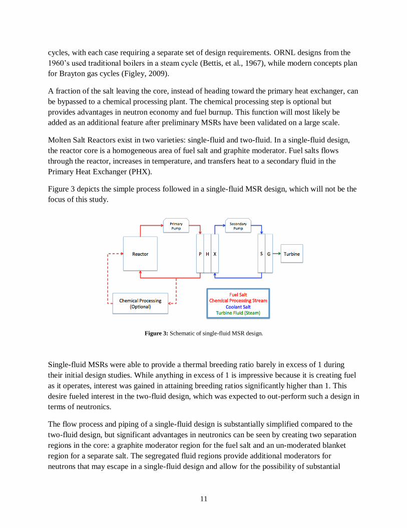
Molten Salt Reactors exist in two varieties: single-fluid and two-fluid. In a single-fluid design,
the reactor core is a homogeneous area of fuel salt and graphite moderator. Fuel salts flows
through the reactor, increases in temperature, and transfers heat to a secondary fluid in the
Primary Heat Exchanger (PHX).
Figure 3 depicts the simple process followed in a single-fluid MSR design, which will not be the
focus of this study.
Figure 3: Schematic of single-fluid MSR design.
Single-fluid MSRs were able to provide a thermal breeding ratio barely in excess of 1 during
their initial design studies. While anything in excess of 1 is impressive because it is creating fuel
as it operates, interest was gained in attaining breeding ratios significantly higher than 1. This
desire fueled interest in the two-fluid design, which was expected to out-perform such a design in
terms of neutronics.
The flow process and piping of a single-fluid design is substantially simplified compared to the
two-fluid design, but significant advantages in neutronics can be seen by creating two separation
regions in the core: a graphite moderator region for the fuel salt and an un-moderated blanket
region for a separate salt. The segregated fluid regions provide additional moderators for
neutrons that may escape in a single-fluid design and allow for the possibility of substantial

12
thermal breeding, which was not viable in a single-fluid design. Fuel processing is not
necessarily required for a two-fluid design as it is for a single-fluid design that hopes to achieve a
breeding ratio in excess of one. With a focus on achieving the highest breeding ratio possible,
momentum shifted to the two-fluid design at ORNL.
A two-fluid design, in contrast to the single-fluid design shown in Figure 3, has separate fluid
streams for the fuel salt and blanket salt. The fuel salt, a uranium-containing FLiBe compound,
differs from the blanket salt, a thorium-containing FLiBe compound, in a two-fluid design. In
order to improve the neutron economy of the reactor design, the blanket regions acts as a
reflector and region to capture any neutrons that would have escaped in a single-fluid design.
The heat produced in this region is lower than in the fuel salt region, but its inclusion is
necessary to cause as much fission as possible. The fuel salt follows a closed path through the
graphite moderator, into the fuel salt pump, down through the Primary Heat Exchanger (PHX),
and back to the moderator region of the reactor core. The blanket salt follows a closed path
through the blanket region, through the blanket pump, into the Blanket Heat Exchanger (BHX),
and back into the blanket region of the reactor core. The secondary coolant salt travelled upward
through the PHX, transferring heat from the fuel salt to the coolant salt, which was then passed
to the BHX, where it picked up the additional heat before moving to the BOP. Figure 4 shows a
diagram of a two-fluid MSR from ORNL in 1968 (Robertson, Smith, Briggs, & Bettis, 1968).
Figure 4: Schematic of two-fluid MSR design from ORNL, courtesy of Oak Ridge National Laboratory (Bettis, et al., 1967).
Progress evolved rapidly at ORNL in the 1960’s when the two-fluid design took control due to
its ability to achieve thermal breeding ratios over 1. As the research developed and matured

13
while being backed by Director Alvin Weinberg, the MSR concept later fell out of favor in the
early-1970’s in favor of the Liquid Metal Fast Breeder Reactor (LMFBR) (LeBlanc, 2010). The
technology remained dormant for nearly 40 years, but recent concerns with LWR designs and
interest in using thorium has led India and China to begin developing MSR designs (Martin,
2011).
Modern domestic design concepts, such as the Liquid Fluoride Thorium Reactor (LFTR), have
begun to garner interest in the MSR technology once again in the United States, but there are no
completed designs with the level of maturity associated with ORNL’s MSBR concept.
Significant funding and research efforts will be required to bring this promising technology to
fruition.
In the time since Alvin Weinberg’s final MSR concept was designed, few innovations have been
made in MSR designs, but the technologies around which the plant was built have grown
dramatically. Advances in materials, computing, chemistry, and fabrication technologies would
now render much of the MSBR design obsolete. The MSR concept that was submitted and
accepted as a Generation-IV concept recently is relatively unchanged from the plant designed to
be the MSBR several decades ago, but updates still need to be made throughout the design.
The materials-related issues with MSRs were studied heavily during the 1960’s but were left
somewhat unresolved with the termination of the MSBR project. As material issues with MSRs
were among the reasons the AEC chose to move forward with LMFBRs, nearly all of those
issues were completely alleviated by the time the Molten Salt Reactor Program ceased to
perform research at ORNL (MacPherson, 1985). Great achievements were made to identify,
design, and invent Hastelloy N, but it still has yet to be proven over the large time frame needed
for reactor components. Modern advanced materials and fabrication techniques should allow for
further improvements in performance.
Licensing will be another issue of difficulty for the MSR, as the NRC has never approved a
commercial liquid-fueled design. Claims of “inherent safety” will obviously not be sufficient in a
final design, but the passive safety systems used on MSRs should show an improvement over the
already impressive LWR track record of safety.
The most important aspect of updating the design is using improved components that have the
advantage of better technologies in their design, analysis, and construction. The use of Finite
Element Analysis (FEA) in the design of components and core behavior should allow for much
more concise results with an added level of comfort in their correctness (Figley, 2009). When
compared to the rudimentary techniques used in the original MSRE and MSBR design, modern
components should perform significantly better, be safer, and allow for more aggressive safety
factors.
Heat exchangers, which are a vital component in the overall efficiency of any plant, have made
rapid developments since the 1960’s. Standard shell-and-tube heat exchangers are currently used

14
throughout the nuclear industry, and have been since the 1960’s, but modern advancements may
provide room for significant improvements. This study focuses on the Primary Heat Exchanger,
which is subjected to extreme environmental conditions that may or may not be suitable for vast
improvements.
Primary Heat Exchanger
Based on encouraging results from the MSRE, the Molten Salt Breeder Reactor (MSBR) was
designed to be the first full-scale, commercial nuclear power plant utilizing molten salt liquid
fuels (Kasten, Bettis, & Robertson, 1966). Shell-and-tube heat exchangers were the preferred
heat exchangers at the time the MSBR was designed, so all heat exchangers in the design were of
the shell-and-tube variety. Two types of molten-salt-related heat exchangers, primary and
blanket, were required for the primary system of a two-fluid MSBR. The primary heat
exchanger, the focus of this study, will be explained and studied in further detail.
The function of the primary heat exchanger is to recuperate heat from the fuel salt carrying the
fissile load to an inert secondary salt. Several secondary heat exchangers are required to convert
a heated secondary salt to water, which is converted to steam in a “boiler.” The BHX is subjected
to very similar conditions as the PHX, and the concept studied in this research will also be
relevant in updating the BHX design where required. Very high efficiency heat conversion is
desired for the primary heat exchanger, as any heat that is not transferred to the secondary salt is
a direct detriment to overall plant efficiency. The MSBR heat exchanger was designed as a shell-
and-tube heat exchanger two-pass vertical exchanger with disk and doughnut baffles (Bettis, et
al., 1967). Four such exchangers were necessary for the four separate heat-exchange loops
employed in the MSBR design. Each heat exchanger was able to remove 528.5 MW of heat from
the core. Figure 5 shows a simplistic sketch of the shell-and-tube PHX taken from Figure 4, with
its imposed boundary conditions, its required header locations, and its general shape more clearly
shown.
Figure 5: ORNL shell-and-tube heat exchanger’s boundary conditions, courtesy of Oak Ridge National Laboratory.

15
The primary heat exchanger of a MSR is subjected to a unique set of conditions that brings forth
several design challenges not encountered in standard heat exchangers. The somewhat corrosive
molten salts, especially at temperatures in excess of 700C, require specialized materials
throughout the system to avoid corrosion, radiation damage, and adverse high-temperature
effects such as creep. For these reasons, Hastelloy N was created and tested for use in Molten
Salt Reactors (Grimes, 1967). Hastelloy N comprised the entire construction of the primary heat
exchanger of the MSBR, each of which was roughly 6.5 feet in diameter and 22 feet in height
(Bettis, et al., 1967). Hastelloy N is a material with limited commercial uses, so it is expected to
be very expensive compared to more common stainless steel alloys. Four heat exchangers of the
previously prescribed dimensions would be a sizeable capital cost for use with any material but
are especially troubling considering the exorbitant cost of Hastelloy N. For this reason, any
manner in which the volume of the heat exchanger could be significantly reduced would be a
step in the direction of making molten salt reactors economically competitive. A reduction in the
amount of material used in that volume is also a vital, and separate, calculation that must be
made.
The progress made at ORNL on the shell-and-tube PHX design will be explained in detail later
in this report. Key design parameters, sketches, and site layout plans were included in the ORNL
documentation and will provide a means for comparing the ORNL design to the design presented
in this study. The amount of research and development performed in the 1960’s and 1970’s at
ORNL conveys the serious interest that MSRs invoked over the decade-long period of their
incubation. The considerations and breakthroughs made in that time period can be enhanced by
utilizing modern compact heat exchangers to more efficiently transfer the requisite heat load.
Compact Heat Exchangers
Shell-and-tube heat exchangers are still the preferred concept in LWRs and many other
applications today, but the compromised efficiency seen with their use may not outweigh their
relatively more advanced operational experience in future designs. Compact heat exchangers,
which use sophisticated fabrication techniques to form extremely small (well below 1mm in
diameter) micro-channels, allow for more complete heat transfer in much smaller volumes
(Ashman & Kandlkar, 2006). Advanced fabrication methods, such as the chemical etching
process used for the Printed Circuit Heat Exchanger (PCHE), allow for small-scale fabrication of
such complex heat exchanger geometries in a manner similar to how computer circuits are
fabricated (Kanaris, Mouza, & Paras, 2004). The use of very small micro-channels allows for
similar heat transfer areas to be accommodated in much smaller total volumes, while using less
solid material in the process.
16
Modern compact heat exchangers can provide compactness, a measure of the ratio of surface
area-to-volume of a heat exchanger, approaching 2500
m2 /m3 for the most advanced designs.
When compared to a compactness of only approximately 43
m2 /m3 for the shell-and tube
designed for the MSBR (6.5 feet diameter and 22 feet height, while accommodating a heat
transfer area of nearly 900
m2) (Kasten, Bettis, & Robertson, 1966), compact heat exchangers
can provide significant reductions in volume and material usage. With tightly packed channels
making adjacent streams able to effectively translate temperatures across their boundaries,
approach temperatures (the difference between the outlet temperature of one fluid stream and the
inlet temperature of the opposing fluid stream at their common header location) closer to 1C are
possible with compact heat exchangers. Shell-and-tube heat exchangers are often closer to 12C
in approach temperature, another demonstration of their inferior performance (Kandlikar,
Garimella, Li, Colin, & King, 2006). Compact heat exchangers are an intriguing technology that
could provide MSRs, and nuclear reactors in general, with a means to reduce capital costs.
Compact Heat Exchanger History
The first sign of movement to relatively “compact” heat exchangers was seen in the automotive
industry in the early 1900’s, when an improved manner for removing heat from engines with
minimal material (weight) was sought. Whereas heat was previously removed from engines by
boiling a pool of water and releasing it into the air in an unsophisticated convection process, heat
exchangers were seen as an inexpensive way to improve engine performance (Shah & Sekulic,
2003).
Automakers began to use closed volumes of liquid arranged in “serpentine” pipes to increase the
heat transfer area and remove the unpredictable boiling process. From this starting point,
engineers have continued to find new ways to increase the performance of automotive radiators
and heat exchangers in countless other industries. With the limits of standard serpentine
arrangements being reached, extended surfaces were then added to more efficiently remove heat,
and pipe geometries were altered to provide improved performance. The automotive industry,
however, had little need for significantly enhanced performance past the designs of the early
1900’s. Several other industries provided a great deal of room for improvement and proved to be
the launching point for the oft-researched compact heat exchanger field (Shah, McDonald, &
Howard, 1980).
Several years of technology advancement on the aircraft internal combustion engine led to a
much better understanding of the physics and abilities of extended surfaces as heat transfer
enhancers. The first compact heat exchanger that resembled anything seen today was made for
the after-cooler of the jet engine during World War II, with enough success and interest shown to
interest the United States Navy Bureau of Ships to begin testing compact heat exchangers on
their gas turbines (Shah, McDonald, & Howard, 1980).

17
The Navy’s work in the 1940’s was extended to research at Stanford University throughout the
next two decades, and that group made several of the most fundamental achievements in
compact heat exchanger design. Culminating with the first publication of works by A.L. London,
who later teamed with W.M. Kays to lead the compact heat exchanger field with their
fundamental texts, the groundwork was laid for the massive improvements that have come with
compact heat exchangers in the decades since work began. The work by the Navy and Stanford
University, coupled with improved computing abilities, helped draw interest from several
industries that could benefit from the advantages offered by more sophisticated heat exchanger
design.
Heat exchanger designs continued to expand and develop through the 1960’s and more industries
gained interest in using compact heat exchangers to increase efficiency. Compact heat exchanger
technologies spread from the automotive industry to the air conditioning industry, several
manufacturing industries, and even to the magnetic railway industry (Shah, McDonald, &
Howard, 1980).
The 1980’s brought an increase in computing power and function that led compact heat
exchanger research away from experimental solutions in favor of Computational Fluid Dynamics
(CFD). CFD provided low-cost means to simulate the physics occurring inside heat exchangers
relatively accurately, without the need to construct and test physical apparatuses before a final
design was developed. It took several years, and decades in some cases, for the computing power
to be able to accurately predict the physics in a timely fashion for the incredibly small geometries
in compact heat exchangers. That breakthrough allowed for significant advancements in the
industry. Optimization processes were more easily obtained, and more complex geometries could
be tested with the use of CFD.
In the time since CFD became prevalent in heat exchanger design, several systems of
commercial codes have been developed to allow for rapid testing and simulations. The programs
continue to be become more accurate, and as computers continue to become more powerful and
swift in their calculations, the use of CFD will expand to new applications.
The technologies available today are leaps and bounds ahead of the resources available to those
designing the MSBR in the 1960’s. Computing power has made hydrodynamics and heat transfer
incredibly more accurate in comparison to hand drawings and manual calculations done in the
initial MSBR design (Bettis, et al., 1967). The computer programs developed at ORNL for
optimization of the heat exchanger designs were rudimentary compared to the commercial
software packages available today. Performing CFD analyses in FLUENT, with automated
optimization available in ANSYS Workbench, is much more sophisticated than the analog
computer models used in the 1960’s for overall plant operation (Burke, 1972) and heat
exchanger design (Bettis, Pickel, Crowley, Simon-Tov, Nelms, & Stoddart, 1971).

18
Compact Heat Exchangers in a MSR
Materials technologies have also come very far since the 1960’s, which may allow for alloys
more advanced than Hastelloy N to be available. Hastelloy N created today can also be
guaranteed to be of greater quality due to the improvement of measuring and manufacturing
techniques. More complex fabrication techniques may allow for corrosion resistant claddings to
be added to inner structural members in order to capture the advantages of low-corrosion
cladding materials with high-strength inner materials such as ceramics. And most importantly,
compact heat exchangers have been developed to allow for more efficient, complete heat transfer
in volumes much less than what was possible in the past. The primary heat exchanger is a perfect
component that can be updated with modern materials, technologies, and analysis to improve an
otherwise obsolete design.
Various studies have been performed in attempts to update the intermediate heat exchanger that
is downstream of the primary heat exchanger, mostly because its performance is strongly tied to
the ability to employ more efficient conversion cycles, such as the Brayton cycle using
supercritical 𝑂 (Harvego, 2006). Updating the unique set of conditions a primary heat
exchanger is subjected to, which shares only a few similarities with those experienced by the
intermediate heat exchanger, will be a valuable study for the future of MSRs. The liquid-to-
liquid primary heat exchanger will come with its own advantages and challenges when compared
to the liquid-to-gas intermediate heat exchanger.
This report will serve as a complete study of the design of a primary heat exchanger for a molten
salt reactor. Using ORNL’s operating conditions as a basis for which the updated heat exchanger
will also function, the compact heat exchanger designs can be fairly compared and contrasted
against the completed shell-and-tube design. A study in materials issues behind each design,
fabrication techniques necessary for each design, and creating a commercially viable means for
implementation of such a design will each be carried out. This thesis will serve to update the
primary heat exchanger design of the MSBR with modern technologies that will allow for
improved performance.
Heat Exchanger Design
Heat exchangers have existed for several decades, and various texts have been written to
summarize standard practices in the design of such heat exchangers. No matter the application,
material, and geometry used, the design of a heat exchanger should be completed in a similar
manner. Classic textbooks exist on exactly this subject and are explained here.
A common approach for heat exchanger design has been developed in recent years to provide a
flowchart for the long and iterative nature of heat exchanger design (Shah & Sekulic, 2003).
Although modern software tools have eliminated the need to manually perform several separate
tasks, the general order of the design process is still followed. In addition to laying out a concise

19
design process for designing any type of heat exchanger, there are also strict classifications for
the different types of heat exchangers. The design process will be presented here but will be
followed directly and displayed in more detail in the body of this report.
The schematic for the heat exchanger design process is displayed below in Figure 6 to emphasize
the complexity and inter-related nature of the steps in the process. In this study, process
specifications are brought from the ORNL study on the Primary Heat Exchanger (Bettis, et al.,
1967). Thermal and hydraulic design is performed in FLUENT. Mechanical design can also be
completed in ANSYS Workbench using the outputs from FLUENT found in previous steps.
Several of the final steps shown in the diagram in Figure 6 (Heat transfer and hydrodynamic
performance, mechanical/structural design, optimized design options, trade off, and system-
based optimization) are amassed in the multiple functions of ANSYS Workbench, including the
Goal-Driven Optimization module. The theory and process behind this portion of the heat
exchanger design is provided later in this report.
Figure 6: Heat exchanger design process (Kays & London, 1984).
In addition to the CFD design that encompasses the majority of Figure 6, manufacturing and
economic considerations must be taken into account to complete a thorough heat exchanger
design. For example, the possibility of casting the heat exchanger designed in this study is
presented later in this report. Testing using ProCast, a Finite Element Analysis (FEA) program
20
that determines the feasibility of casting geometries with the proposed materials, is still needed
to validate such a concept.
The process laid out in Figure 6 has been simplified by the ability of ANSYS Workbench to
build, simulate, change, and optimize fluids and heat transfer problems. With manual input of the
design specifications, ANSYS Workbench can provide accurate, optimized results on a
significantly shortened time scale. Fundamental heat exchanger design texts were still vital in
demonstrating a consistent process and identifying the numerous considerations that must be
made.
II. Literature Review Comprehensive resources are available for all aspects of the design of an advanced heat
exchanger in the form of textbooks, educational papers, and formal project reports. The sources
fell into three categories: compact heat exchanger basics, related ORNL studies, and compact
heat exchangers in the nuclear industry.
Compact Heat Exchanger Basics
Several text sources cover specialized applications in compact heat exchangers that more
thoroughly explain the nuances of the advanced designs and theory related to compact heat
exchangers. In addition to outlining several key considerations and physical processes, these
texts tend to look to the future by mentioning advanced concepts that may allow for improved
performance. The following texts cover studies involved with the advanced compact heat
exchanger designs being considered.
Fundamental texts have been written on the specialized scope of compact heat exchangers, which
cover the key advancements in the industry and focus on the design issues that arise on the small
scale in which they exist (Kays & London, 1984). Various issues arise in compact heat
exchangers that are not present in shell-and-tube exchangers, which would provide especially
challenging designs for use in the nuclear industry.
Of interest in this study are pure counter-flow compact channel heat exchangers, which can also
be classified as “direct-transfer, indirect-contact” exchangers. This type of heat exchanger is
characterized by two fluids transferring heat between each other without the fluids coming into
direct contact. This type of heat exchanger is also known as a recuperator, describing the
requirement to recover as much heat as possible from one fluid to the next. The current design
also falls under “prime surface exchanger”, where no fins or extended surfaces are added to the

21
channels. Figure 7 shows the entire classification procedure used for heat exchangers with each
category the heat exchanger in this study falls under shown in red.
Figure 7: Classification procedure for heat exchangers, with the slotted minichannel shown in red (Kays & London, 1984).
As shown in Figure 7, a liquid-to-liquid exchanger must have a surface area density of 400
in order to be considered “compact”. If the heat exchanger designed in this study does
not provide a significant upgrade in compactness and decrease in material usage, the
complexities of using such a heat exchanger would not be warranted. Performing at a level
sufficient to use the term “compact” heat exchanger will not be an issue in this study.
Correlations for channels of rectangular cross-section are provided for Nusselt number and
Poiseuille number, which will be discussed later in this report as part of the process of validating
the CFD model used in this study. Other similar correlations are available for “Plain Plate-Fin
Surfaces”, which are plate-type heat exchangers that omit surface features and roughly resemble
the rectangular cross-section channels that are the focus of research in this study. These studies
show experience with rectangular channels in compact heat exchanger applications, but the
specific boundary conditions prescribed in this study will not match the simple situations
presented in the correlations (constant wall temperature and constant heat input on outer fluid
surface). The correlations found for the physics in this study, which use an outer constant
temperature boundary condition surrounding a finite array of channels, will be presented in the
Results section of this report.

22
The calculations used in the Parameter Set of ANSYS Workbench shown in the Set Up section
of this report are based on common heat exchanger parameters found in fundamental texts (Kays
& London, 1984). The ε-NTU (Number of Thermal Units) and LMTD (Log-Mean Temperature
Difference) methods are presented in detail, with the latter being exercised in this study.
The channel dimensions proposed in this research will fall within the “Minichannel” range due to
restrictions on maintenance, which will invalidate microchannels (Kandlikar, Garimella, Li,
Colin, & King, 2006). Channel sizes on the conventional range without surface features do not
perform adequately well to justify their use in place of a shell-and-tube heat exchanger. The
Minichannel range, especially at channel heights between 0.5mm and 2mm, is expected to be in
the optimal range of balance between performance and maintenance. Table 2 displays the ranges
of compact heat exchanger classifications by the size of the channel (Kandlikar, Garimella, Li,
Colin, & King, 2006).
Table 2: Heat exchanger channel classification by size of hydraulic diameter (Kandlikar, Garimella, Li, Colin, & King, 2006).
Channel Classifications
Conventional Channels D > 3 mm
Minichannels 3 mm ≥ D > 200 µm
Microchannels 200 µm D > 10 µm
Transitional Microchannels 10 µm ≥ D > 1 µm
Transitional Nanochannels 1 µm ≥ D > 0.1 µm
Nanochannels D ≤ 0.1 µm
An intriguing benefit that launched studies into a high-aspect-ratio, “slotted,” design is the high
Nusselt number seen in such channels. Nusselt number, which correlates directly to the heat
transfer coefficient for a given arrangement and generally compares the contributions of
convective and conductive heat transfer, is an important value in considering the heat transfer
performance of a design. With the effect of the Nusselt number on heat transfer performance
considered to be greater in a final design than the Poiseuille number on pressure drop, an
increase in the Nusselt number compared to a circular channel is attractive. Table 3 shows the
effect of changing a rectangular channel’s aspect ratio on its heat transfer performance and
pressure drop, and also serves to compare those values to those for circular channels (Kandlikar,
Garimella, Li, Colin, & King, 2006).
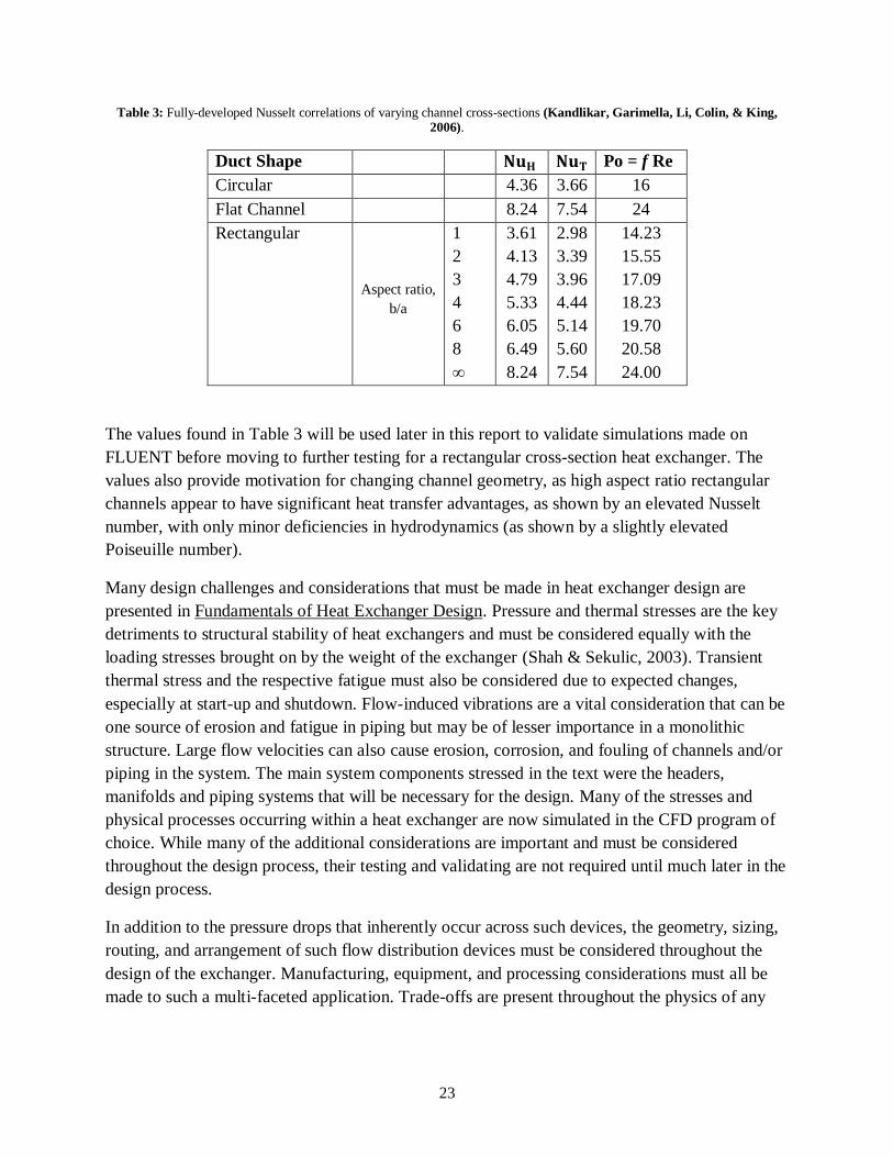
23
Table 3: Fully-developed Nusselt correlations of varying channel cross-sections (Kandlikar, Garimella, Li, Colin, & King, 2006).
Duct Shape Po = f Re
Circular 4.36 3.66 16
Flat Channel 8.24 7.54 24
Rectangular
Aspect ratio,
b/a
1
2
3
4
6
8
∞
3.61
4.13
4.79
5.33
6.05
6.49
8.24
2.98
3.39
3.96
4.44
5.14
5.60
7.54
14.23
15.55
17.09
18.23
19.70
20.58
24.00
The values found in Table 3 will be used later in this report to validate simulations made on
FLUENT before moving to further testing for a rectangular cross-section heat exchanger. The
values also provide motivation for changing channel geometry, as high aspect ratio rectangular
channels appear to have significant heat transfer advantages, as shown by an elevated Nusselt
number, with only minor deficiencies in hydrodynamics (as shown by a slightly elevated
Poiseuille number).
Many design challenges and considerations that must be made in heat exchanger design are
presented in Fundamentals of Heat Exchanger Design. Pressure and thermal stresses are the key
detriments to structural stability of heat exchangers and must be considered equally with the
loading stresses brought on by the weight of the exchanger (Shah & Sekulic, 2003). Transient
thermal stress and the respective fatigue must also be considered due to expected changes,
especially at start-up and shutdown. Flow-induced vibrations are a vital consideration that can be
one source of erosion and fatigue in piping but may be of lesser importance in a monolithic
structure. Large flow velocities can also cause erosion, corrosion, and fouling of channels and/or
piping in the system. The main system components stressed in the text were the headers,
manifolds and piping systems that will be necessary for the design. Many of the stresses and
physical processes occurring within a heat exchanger are now simulated in the CFD program of
choice. While many of the additional considerations are important and must be considered
throughout the design process, their testing and validating are not required until much later in the
design process.
In addition to the pressure drops that inherently occur across such devices, the geometry, sizing,
routing, and arrangement of such flow distribution devices must be considered throughout the
design of the exchanger. Manufacturing, equipment, and processing considerations must all be
made to such a multi-faceted application. Trade-offs are present throughout the physics of any
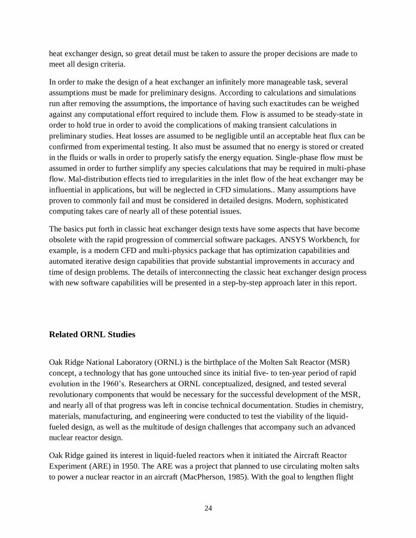
24
heat exchanger design, so great detail must be taken to assure the proper decisions are made to
meet all design criteria.
In order to make the design of a heat exchanger an infinitely more manageable task, several
assumptions must be made for preliminary designs. According to calculations and simulations
run after removing the assumptions, the importance of having such exactitudes can be weighed
against any computational effort required to include them. Flow is assumed to be steady-state in
order to hold true in order to avoid the complications of making transient calculations in
preliminary studies. Heat losses are assumed to be negligible until an acceptable heat flux can be
confirmed from experimental testing. It also must be assumed that no energy is stored or created
in the fluids or walls in order to properly satisfy the energy equation. Single-phase flow must be
assumed in order to further simplify any species calculations that may be required in multi-phase
flow. Mal-distribution effects tied to irregularities in the inlet flow of the heat exchanger may be
influential in applications, but will be neglected in CFD simulations.. Many assumptions have
proven to commonly fail and must be considered in detailed designs. Modern, sophisticated
computing takes care of nearly all of these potential issues.
The basics put forth in classic heat exchanger design texts have some aspects that have become
obsolete with the rapid progression of commercial software packages. ANSYS Workbench, for
example, is a modern CFD and multi-physics package that has optimization capabilities and
automated iterative design capabilities that provide substantial improvements in accuracy and
time of design problems. The details of interconnecting the classic heat exchanger design process
with new software capabilities will be presented in a step-by-step approach later in this report.
Related ORNL Studies
Oak Ridge National Laboratory (ORNL) is the birthplace of the Molten Salt Reactor (MSR)
concept, a technology that has gone untouched since its initial five- to ten-year period of rapid
evolution in the 1960’s. Researchers at ORNL conceptualized, designed, and tested several
revolutionary components that would be necessary for the successful development of the MSR,
and nearly all of that progress was left in concise technical documentation. Studies in chemistry,
materials, manufacturing, and engineering were conducted to test the viability of the liquid-
fueled design, as well as the multitude of design challenges that accompany such an advanced
nuclear reactor design.
Oak Ridge gained its interest in liquid-fueled reactors when it initiated the Aircraft Reactor
Experiment (ARE) in 1950. The ARE was a project that planned to use circulating molten salts
to power a nuclear reactor in an aircraft (MacPherson, 1985). With the goal to lengthen flight

25
times indefinitely, the Air Force saw nuclear-powered aircraft as the flying equivalent to the
nuclear submarine fleet the Navy was in the process of developing (LeBlanc, 2010). Interest in
the aeronautical applications for molten salt reactors waned, but the technology showed enough
promise during the ARE that research was launched into harnessing those abilities for civilian
nuclear power from molten salts. ORNL Director, Alvin Weinberg, the foremost supporter of
Thorium and molten salt technologies, proposed that the knowledge gained from the ARE be
translated to an electrical-power-producing molten salt reactor.
As molten salt-related concepts continued developing, greater concentration was focused on the
possibility of thermal breeding. The concept of a nuclear reactor being able to create its own fuel
was intriguing for obvious reasons, so the 1960’s saw a renewed interest in realizing the full
potential of a thermal breeder reactor (MacPherson, 1985). The next step in ORNL’s MSR
reactor design culminated in the Molten Salt Reactor Experiment (MSRE), a step towards
commercial relevance that remains perhaps the most influential researching tool ever created for
the MSR technology.
ORNL launched the Molten Salt Reactor Experiment (MSRE), a single-fluid molten salt test
reactor that produced just 8 MW of thermal power, in the early 1960’s. With the creation of
Hastelloy N, then called “INOR-8” during its developmental phase, corrosion issues with the
molten salts were mostly mitigated. The MSRE was operated for five years to test materials,
system components, and the stability of the reactor’s operation.
While no issues were encountered during the entire operating life of the MSRE, corrosion found
in the MSRE loop was enough to cast serious doubts for the long-term viability of molten salt
reactors. Although the root of the corrosion issues was studied and believed to be found by the
time of its cancellation, the Atomic Energy Commission (AEC) decided to cease major
investments in MSRs (MacPherson, 1985). Liquid Metal Fast Breeder Reactors (LMFBRs) came
in favor with the AEC and began their development, which proved to be the end of Molten Salt
Reactor development.
Before research was halted on MSRs, ORNL conducted several studies on the design of the heat
exchangers necessary in the MSR, including several detailed studies of the Primary Heat
Exchanger (PHX). Many of the key design considerations brought forth by ORNL engineers
during the design of their shell-and-tube PHX are addressed here and will play a vital role in the
ability of any advanced PHX design to become feasible in power plant applications. In a similar
process, albeit with much more advanced technology available than in the 1960’s, this study will
develop a PHX for the modern MSR. ORNL resources are available for the shell-and-tube heat
exchanger design that was planned for the Molten Salt Breeder Reactor (MSBR), which will be
used as the baseline design for this study.
ORNL conducted studies solely geared towards designing the heat loops and required systems
for the MSBR. The PHX was a major component in several of such studies, and the evolution of

26
its design is well documented (Bettis, et al., 1967). This document, written and produced in
1967, did not have the modern advancements to analyze and design more complex designs than
shell-and-tube heat exchangers. Hand-written calculations were augmented by small-scale
experimental results to provide approximate values for design calculations. Thorough discussion
of the considerations to be made for such a heat exchanger was provided, and will be a vast
resource for similar concepts in the heat exchanger resulting from this study.
The work completed on the heat-exchange system of the MSBR was preceded by in-depth
studies of reactor core characteristics and behavior that validated further work on molten salt
reactor plant design. In order to understand the implementation of a Primary Heat Exchanger
(PHX) in the broad scope of a molten salt reactor plant, a complete design of the MSBR concept
must be explained.
The two-fluid MSBR design used four identical heat loops, each having one Primary Heat
Exchanger, one Blanket Heat Exchanger, four boilers, two steam reheaters, and two reheat-steam
pre-heater. Each loop carried 25% of the total plant load from the single 1000-MW(e) reactor.
The modular nature of this design was conceptualized to allow for easier repair and removal of
system components, such as the heat exchangers.
The reactor contained two separate regions: the graphite moderating region in the center of the
core and the blanket region on the outside of the core. Fuel salt flows upward through channels
in the graphite, where fission takes place and is controlled by the moderator. The blanket region
reflects neutrons and produces some heat by fission itself.
The fuel salt leaves the bottom of the reactor at 1300°F, enters on the side primary heat
exchanger near the top of its height, flows downward through the tubes of the PHX, and is
cooled to 1000°F as it leaves from the side near the middle of the PHX’s height. The cooled fuel
salt is then returned to the reactor to be heated again.
The PHX is designed as a two-pass shell-and-tube heat exchanger with disk and doughnut
baffles. The fuel salt flows downward through the tubes in the outer region of the heat exchanger
and then flows upward through the tubes in the center region (Bettis, et al., 1967).
The blanket salt enters the reactor at 1150°F on the side of the reactor, flows in both directions
around the moderator, is heated up to 1250°F, and leaves the reactor at nearly the same point it
entered (Bettis, et al., 1967). Heat is removed from the blanket salt, and thus transferred to the
secondary salt, by means of a blanket heat exchanger (BHX). The BHX and its necessary design
is very similar to the PHX but has been ignored. After leaving the BHX and having its heat
removed by the inert secondary salt, the blanket salt can once again re-enter the blanket region of
the reactor at 1150°F.
Coolant salt enters the PHX at 850°F, flows countercurrent to the fuel salt through the PHX, and
leaves at 1111°F. The pre-heated coolant salt then enters the bottom of the BHX, is heated by the

27
blanket salt, and leaves the top of the BHX at 1125°F. The coolant salt then is pumped to the
secondary system, where it is used to perform two functions: to create steam in the boiler (87%
of flow) and to reheat exhaust steam from high-pressure turbine (13% of flow). The coolant salt
is then returned to its initial 850°F and re-enters the PHX to once again repeat the cycle. Figure 8
shows the entirety of one MSBR design created at Oak Ridge in the 1960’s, which employs a
two-fluid design attached to a steam cycle for Case A (an early PHX concept that was later
improved and evolved into Case B).
Figure 8: MSR plant diagram showing boundary conditions, courtesy of Oak Ridge National Laboratory (Bettis, et al., 1967).
Two options for the PHX were considered, each of which have separate fuel salt and blanket salt
sections, in addition to the secondary coolant salt. The design of each option was optimized and
designed simultaneously, then contrasted at the end of ORNL’s study.
The PHX designed in Case A planned for the fuel salt to leave the reactor and flow downward
through the tubes in the outer section of the heat exchanger, flow upward through the tubes in the
inner annulus, and return back to the reactor from the top of the PHX. The coolant salt flows in
the opposite direction as the fuel salt on the shell-side of the heat exchanger. Coolant salt also
enters at the top of the PHX, flows downward through the center section of the heat exchanger,
flows upward through the outer section, and flows to the inlet of the blanket heat exchanger from
the top of the PHX.

28
Figure 9 shows the original PHX design (Case A) planned for the MSR, with arrows showing the
direction of fluid flow.
Figure 9: Shell-and-tube heat exchanger for Case A of MSBR design, courtesy of Oak Ridge National Laboratory (Bettis, et al., 1967).
Case A had issues arise when it required reheat-steam preheaters to raise the temperature of
exhaust steam from the high-pressure turbine. Case B was developed to preclude the necessity
for such a device. Case B also alleviated several issues that arose in the utilization of Case A’s
PHX, most importantly where operating pressures of the fuel salt were found to be higher than
operating pressures of the coolant salt at similar points in the heat exchanger. This would cause
fuel salt to leak into the coolant salt, in the event of a tube rupture, which would spread
radioactive material to the secondary side of the plant. This issue was eliminated in Case B in
favor of a more balanced pressure distribution (Bettis, et al., 1967). In making these changes, an
advantage was seen in pressure distributions of the salts in the core. Lower pressures of the fuel
salts were found throughout the core after the resulting design changes, especially in the areas
where salts came in contact with the graphite moderator.
In the process of changing and rearranging the heat exchanger internals, the fluid inlets and
outlets were altered slightly to adapt to the new layout. The difference is clear when comparing
Figure 9 with the plant diagram of Case B shown in Appendix A.
Several changes were also required to the balance of the heat-exchange system due to the
changes made in the change from Case A to Case B. All heat exchangers downstream of the
PHX required slightly different temperatures and pressures to account for the changes in the
system. The resulting system configuration is found in Appendix A.

29
Figure 10: Shell-and-tube heat exchanger for Case B of MSBR design, courtesy of Oak Ridge National Laboratory (Bettis, et al., 1967).
Fluid flows were reversed in Case B, as opposed to how they were designed in Case A. In the
Case B PHX, fuel salt enters in the center section at the top of the heat exchanger, flows
downward through the tubes in the center section, flows upward through the tubes in the outer
section, and leaves toward the reactor at the top of the heat exchanger. Coolant salt enters at the
top of the heat exchanger in the outer region, flows downward through the baffles on the shell-
side, flows upward through the baffles in the inner section, and then leaves toward the BHX at
the top of the heat exchanger.
Table 4 provides the design parameters seen in each heat exchanger system and a description of
the shell-and-tube design. These values will serve as the guidelines for which the new heat
exchanger will be designed, in order to best contrast the compact heat exchanger design with a
previously accepted design. The heat exchanger was made entirely of Hastelloy N, which at a
size as immense as all four were planned to be, would be quite a capital expense.
Performance characteristics and geometric quantities were taken from this table to provide a
concise means to which results from the compact heat exchanger can be compared. The results of
such calculations will be presented later.

30
Table 4: Characteristics of ORNL’s final shell-and-tube heat exchanger design (Bettis, et al., 1967).
Type Shell-and-tube Shell thickness (in)
1
two-pass vertical
exchanger
Shell ID (in)
Number required
4 Center section
40.25
Annular section 66.7
Rate of heat transfer, each
MW
528.5 Tube sheet material Hastelloy N
BTU/hr
1.8046 x 10^9
Tube sheet thickness (in)
Shell-side conditions
Top outer annulus
1.5
Cold Fluid
Coolant salt Top inner annulus
2.5
Entrance temperature (F)
850 Floating head
3.5
Exit temperature (F)
1111
Entrance pressure (psi)
198 Number of tubes
Exit pressure (psi)
164 Inner annulus
4347
Pressure drop across exchanger (psi)
34 Outer annulus
3794
Mass flow rate (lb/hr)
1.685E07
Pitch of tubes (in)
Tube-side conditions
Center section
0.600
Hot fluid
Fuel salt Annular section
0.625
Entrance temperature (F)
1300
Exit temperature (F)
1000
Total heat transfer area per exchanger
(ft^2)
Entrance pressure (psi)
146 Center section
4875
Exit pressure (psi)
50 Annular section
4790
Pressure drop across exchanger (psi)
96 Total
9665
Mass flow rate (lb/hr)
1.093E07
Basis for area calculation
Tube OD
Mass velocity (lb/hr*ft^2)
Center section
5.95*10^6 Type of baffle
Disk and
doughnut
Annular section
5.175*10^6
Number of baffles
Velocity (ft/sec)
Center section
4
Center section
13 Annular section
10
Annular section
11.3
Overall heat transfer coefficient
Tube material
Hastelloy N BTU/(hr*ft^2)
1106
Tube OD (in)
0.375 Maximum stress intensity (psi)
Tube (Calculated)
6504
Tube thickness (in)
0.035 Tube (Allowable)
17500
Tube length (tube sheet to tube sheet, ft)
Shell (Calculated)
9945
Inner annulus
15.286 Shell (Allowable)
56250
Outer annulus
16.125
Maximum tube sheet stress (psi)
Shell material
Hastelloy N Inner annulus
3500
Outer annulus 17000
A list of considerations and design factors was also made in the ORNL documentation (Bettis, et
al., 1967) as a means for assuring that the heat exchanger design was of the quality necessary for
its application. Although many of the considerations were made with a shell-and-tube heat
exchanger in mind, the thoughts were valid and remain relevant for the compact heat exchanger
of interest in this study.
The development of corrosion-resistant materials had already taken place at ORNL, and its use
throughout the plant was considered. All metal surfaces that come in contact with the molten

31
fluorides in the MSBR system were required to be made of Hastelloy N, while other surfaces at
elevated temperatures must have considerations made to address those points.
Just as maintenance is a large focus of the design of the compact heat exchanger in this study, the
engineers at ORNL considered maintenance philosophy largely. The concept of using four
separate trains, with separate heat exchangers for each loop, is a step in the process of becoming
“modular” for ease of replacement and maintenance. In addition to making replacement easier
with hot cells and smaller banks of heat exchanger modules, rather than making repairs in place,
standard shell-and-tube exchanger maintenance philosophies are carried through to this design.
Standard maintenance and cleaning procedures were carried from other shell-and-tube, but
compact heat exchangers will require that new, innovative processes be developed.
All calculations by ORNL were performed manually, without the assistance of computers to
provide three-dimensional modeling capabilities until much later. More complex, thorough
models will be able to be performed now with the current technologies available using Finite
Element Analysis (FEA). Automated, accurate optimization will make for heat exchangers with
even greater performance.
Compact Heat Exchanger Developments
In addition to the reports provided under large research programs that have been under way in
recent years, several educational papers have been written covering the analytical aspects of
compact heat exchanger design. Whereas project reports have a focus on creating heat
exchangers for a test apparatus or a full-scale application, the more specialized technical papers
cover different, albeit similarly important, aspects of the heat exchangers. The study and
development of heat exchanger correlations and advanced methods of computation developed in
these papers and texts has been vital in the advancement of compact heat exchangers. Several of
these sources will be presented here.
A comprehensive text about one type of compact heat exchanger, the plate-type heat exchanger
(PHE), has been developed to introduce the wealth of options available for construction of this
type of heat exchanger (Wang, Sunden, & Manglik, 2007). Plate-type heat exchangers are named
for the manner in which they are produced, where plates are stacked directly on top each other to
create the cross-section of the heat exchanger channels. Bonding techniques are required for
plated to adhere to one another, which is often achieved by brazing or welding. This requirement
brings forth a weakness in the mechanical integrity of the system and may be able to be
eliminated with casting techniques. Although the manner in which the channels are produced
may differ in the results presented later in this report, the findings for channel sizes and shapes
remain relevant for any compact heat exchanger.

32
There are many different types of fabrication methods that are categorized under plate-type heat
exchangers: brazed plate, fully welded, wide-gap, double-wall, diabon graphite, and minex plate
heat exchangers. Each type was specifically designed for different temperature and pressure
restrictions, none of which are desired in a molten salt reactor.
Many plate-type heat exchangers use gaskets to connect plates, which would render them useless
in high-temperature nuclear applications. The text mentions that plate heat exchangers can be 20-
30% of the size of standard shell-and-tube heat exchangers, which would obviously present a
large improvement in capital costs. Table 5 displays a comparison of abilities of a Gasketed
PHE, a plate-type heat exchanger with plates joined by gaskets at their interface, compared to a
shell-and-tube heat exchanger.
Table 5: Comparison of Gasketed Plate Heat Exchanger with shell-and-tube heat exchanger (Wang, Sunden, & Manglik, 2007).
Gasketed PHE Shell-and-tube HX
Direct fluid contact Impossible Possible
Approach ~1°C ~5°C
Multiple duty Possible Impossible
Piping connections From one
direction
From several
directions
Heat transfer ratio ~3-5 1
Operating weight ratio 1 ~3-10
Hold-up volume Low High
Space ratio 1 ~2-5
Welds None Welded
Sensitivity to
vibrations
Not sensitive Sensitive
Gaskets On every plate On each bonnet
Leak detection Easy to detect Difficult to detect
Access for inspection On each side of
plate
Limited between
tubes
Disassembly time ~15 minutes ~60-90 minutes
Repair Easy to replace
plates and gaskets
Tube plugging
hurts performance
Thermal size
modification
Easy, add or
remove plates
Difficult
Fouling ratio ~0.1-0.25 1
Welds and gaskets have been replaced recently by more robust ways of connecting plates, such
as diffusion bonding, but the idea of using very small channels manufactured by stacking
similarly shaped plates remains valid. More sophisticated bonding techniques will be necessary

33
to provide ample strength at such high temperatures, but manufacturing the modules as plates
would simplify manufacturing, allowing for commercial production. Although the fabrication
method may differ from those presented in the text, some intriguing plate-type heat exchanger
designs were presented.
The wide-gap plate heat exchanger was presented in this reference and is an intriguing design
that has similarities with the heat exchanger designed in this study. Wide-gap PHEs are often
used in applications where clogging may become an issue, such as some juices in sugar mills and
paper mills. The wide-gap PHEs presented in the reference, which are designed by Alfa Laval,
have complex surface corrugations and wavy patterns to enhance heat transfer. Such surface
features will be removed for the purposes of this study, but the existence of such an intermediate
design confirms that a concept that falls between very compact micro-channel heat exchangers
and shell-and-tube heat exchangers is valid.
Modern achievements in the development of compact heat exchangers have been brought
together in text form to review the possibilities contained by the devices (Sunden & Shah, 2007).
This reference introduced several different types of compact heat exchangers, with a great deal
of detail in new fabrication techniques. This book acknowledges molten salts as a possible
working fluid in compact heat exchangers and introduces some concepts that could be
compatible.
Several issues still exist with ceramic heat exchangers, with the most pressing needs being the
following: ceramic tubes are expensive, long tubes with constant shape and properties are
difficult to fabricate, tube-to-tube sheet joints are not yet leak-tight with current fabricating
techniques, durability in corrosive environment is yet to be confirmed, the coefficient of thermal
expansion may change with time, and mechanical properties of ceramics are not very well
known at this time. It seems that many of the issues with ceramic heat exchangers involve
manufacturing and materials, rather than heat transfer and/or fluid flow. These concerns will
delay the time frame in which ceramics are viable in heat exchanger designs, so the use of such
materials will not be studied in this report.
Significant effort and research have gone into purely theoretical studies that intend to optimize
surface features in compact heat exchangers (Kanaris, Mouza, & Paras, 2004). The report covers
modern enhancements in compact heat exchanger channel geometry technology that can now be
modeled on computers in CFD programs. Significant research has been completed to optimize
the addition of corrugations, each of its own channel aspect ratio, corrugation aspect ratio, and
angle of attack, in order to best enhance heat transfer and minimize pressure drops. The focus of
this study will not include such features, but future iterations can employ them if maintenance is
still deemed reasonable.
The studies presented in this source have shown that drastic improvements in heat transfer
coefficient and heat transfer area can be achieved by including surface corrugations on the inside

34
of the channels, while only modest increases in pressure drops are seen. Several reports have
been written on different processes by which optimization can be achieved for different shapes
and sizes of corrugations, but this will not be the focus of this report. If a simple, un-optimized
compact heat exchanger can perform at a level near that of well-known shell-and-tube heat
exchangers, it should be clear that such a technology holds significant promise in the future.
Although the heat exchanger design in this study will not take advantage of the complexities that
can make compact heat exchangers incredibly efficient, the possibility exists to add such features
to increase performance.
Nuclear-related Compact Heat Exchanger Research
Interest in high-temperature applications in the nuclear power industry have led to research
involving the use of molten salts as secondary coolants. Interest in pairing advanced nuclear
reactors with the Brayton power cycle has led to research on intermediate heat exchangers (IHX)
that transfer heat from a molten salt coolant to helium or super-critical
CO2. Although the results
of these studies are not directly applicable to a study of the PHX, the processes and
considerations made for the design of each heat exchanger are similar. The following reports
were investigated for applicable information.
A cooperative research effort between MIT and Heatric, a compact heat exchanger design
company, was based on their Printed Circuit Heat Exchanger (PCHE) design and produced an
early set of results for high-temperature compact heat exchangers (Gezelius, 2004). The specific
design in this paper was for an intermediate helium-to-helium heat exchanger, but several key
considerations and concepts will hold true for all nuclear-based heat exchanger design.
A key part of this paper was the header design created by Heatric that included built-in headers.
The multi-ported printed circuit heat exchanger (MP PCHE) would have less mal-distribution
effects, better fabrication techniques, easier assembly, and less associated piping. The ability to
construct the header in a similar “plate-type” manner to the rest of the heat exchanger
construction is an advantage in construction and fabrication, and its effects of minimizing
pressure drop are yet another reason to pursue a similar concept.
Most of the work referenced was properly modeling the wavy channels used by Heatric to
optimize heat transfer while minimizing pressure drop. Heatric has not made their proprietary
design public and there was not a readily available heat exchanger for testing, so the author had
to work to create a reasonably similar computer model that could be used to perform
optimization and sensitivity analyses. Due to not knowing exact information for many of the
design parameters used in his study, the author does “optimistic”, “mean”, and “pessimistic”
evaluations for each case. In the end, the PCHE was found to be superior to all other designs,
with the only modest disadvantage being in slightly increased pumping power (due to a slightly
higher pressure drop).

35
For the PCHE, the maximum size for a module was listed at 600mm in height, 600mm in width,
and over 1.5m in length. These constraints may have changed since 2004 and will differ for other
manufacturing methods and locations, but it gives a rough estimate of how large heat exchangers
can be made for that fabrication method. The diffusion bonding process used to join plates
provides a monolithic structure of the same strength as the parent material, so creep will not be
an issue. While avoiding such a process with a monolithic casted structure would be optimal for
the design presented in this thesis, diffusion bonding remains a viability possibility for joining
sections if complete casting is not possible. Heatric aims to make the incurred pressure drop ~1%
of the operating pressure of the system, a viable value to use for all designs with different
pressure values.
Wavy channels, especially of the extremely small scale that these were made for the PCHE, are
not similar to the design points used in this study. The performance of the PCHE may be better
than the slotted design explained in this thesis, but the issue of maintenance could be
insurmountable for designs similar to the PCHE. The slotted minichannel heat exchanger design
introduced later in this thesis will take into account such details.
Idaho National Laboratory (INL) completed a significant amount of work on several high-
temperature heat exchangers as far back as 2006, when studies were conducted on three heat
exchangers (the first heat exchanger downstream of the reactor, the heat exchanger that connects
the balance of plant to the Hydrogen production loop, and a secondary heat exchanger that may
or may not be necessary), none of which apply to research with a MSR’s PHX (Harvego, 2006).
The design is used for a very high-temperature reactor, so explanations for increasing the overall
reactor temperatures are included. The paper describes the outlet temperature as the most
influential parameter for determining overall heat transfer efficiency in the design. Overall plant
efficiencies of up to 51.4% have been postured for plant temperatures up to 950°C, a stark
improvement over current LWR efficiencies. The author explained the operating limits of a
PCHE to be compactness of up to 2500 , operating temperature up to 900°C, and
operating pressure of up to 50 MPa.
A heat exchanger effectiveness of 95% was required for each potential design, and then the
design parameters were altered to optimize other heat exchanger characteristics. The inlet and
outlet parameters were seen as more flexible than allowing for poor performance, which is an
interesting outlook to take on any heat exchanger design. The operating conditions prescribed by
ORNL are more rigid than those explained in the INL design, so such an outlook will not be
possible for the work presented in this thesis. A temperature difference of 360°C in the core was
used for all designs, while higher temperature drops may be possible in future designs. The
author also considered raising the operating pressure to around 3 MPa in a PCHE, in order to
decrease the required pumping power. This is still a relatively low pressure compared to current
LWR conditions, and is well within the 50 MPa limit for PCHEs.

36
More recent work has been performed at Idaho National Laboratory that also covers the design
of an intermediate Helium-Helium heat exchanger for the High Temperature Gas-Cooled
Reactor (Mizia, 2008). Although the precise design and requirements differ for this specific heat
exchanger and plant design, some valuable information was gathered from this report.
The study was restricted mostly to a multitude of possible metal alloys, but also considered
foam, capillary, and ceramic heat exchanger designs. There was an excellent introduction with
different heat exchanger possibilities listed, and the report even goes into detail about current and
past reactors of similar designs. Concepts involving multi-temperature-stage construction and
modular heat exchanger banks were presented and considered for the PHX. Multiple temperature
stages would allow for different alloys to provide their respective advantages as required
throughout the heat exchanger. Alloy 617 is proposed for the high-temperature section due to its
excellent performance at high temperatures and increased resistance to corrosion, while Alloy
800H can be used for the low-temperature section of the heat exchanger that will not be under
such harsh conditions. The possibility of using modular sections to construct the heat exchanger
was briefly mentioned but only as an interesting concept for the future. Although the concept of
only using rare alloys for the high-temperature section of the heat exchanger where its use is
required, the design challenges in manufacturing and differential thermal expansion may be
prohibitively serious. The concept may also not be practical when testing requires Loss of
Coolant Accident (LOCA) simulation, as would be required during commercial plant designs.
LOCA simulation would bring all temperature channels to elevated temperatures that would
render the low-temperature material insufficient. These practices must be accounted for in all
heat exchanger designs and seem to prohibit multiple-stage construction from being a valid
design.
The above study had a primary focus on corrosion and its effect on the system and was found to
be potentially life-limiting at high temperatures. Hastelloy XR, which is used in Japanese High-
Temperature Test Reactor (HTTR), was mentioned as a possible corrosion-resistant material that
may be an option for cladding over a stronger base material.
Eight types of heat exchangers were explained and evaluated on parameters such as
compactness, maturity, stress behavior, and sensitivity to corrosion. Tubular and plated-stamped
Intermediate Heat Exchanger (IHX) designs were chosen for further evaluation and testing.
Minor details from experimental results were introduced, with one pertinent observation
regarding the operating shape of the channel being quite interesting. Originally square in cross-
section, the channels were found to be slightly trapezoidal during operation due to the high
temperature change. This is a somewhat drastic change that could be designed for in the future
and also represents one of several design changes that will be incurred when moving from CFD
simulations to experimental setups. The effects seen from extremely high temperatures changes
cannot be discounted in experimental testing.

37
The progress made among the consortium designing the Intermediate Heat Exchanger (IHX) for
the Next Generation Nuclear Plant (NGNP) has been well-documented and provides a wealth of
knowledge on recent advancement in compact heat exchangers (Hechanova, 2007). The project
focuses on very high-temperature reactors that would function to produce Hydrogen as a result of
its high-temperature fluid streams, with electrical production also being a vital byproduct of the
system. Among the groups working together on the project are the University of California –
Berkeley (UCB), the University of Nevada Las Vegas (UNLV), General Atomics (GA), and
Ceramatec Inc. This particular Progress Report was relatively far along in the development
process, so extended work has been contributed by each party.
The UNLV group has identified three possible types of heat exchangers (Ceramatec compact
heat exchanger, bayonet-type, and shell-and-tube) for comparison. Heat transfer and stress
analyses were performed numerically for the heat exchangers, while the use of different metal
alloys was the focus of the study.
UCB studied the use of ceramics (CSiC/C composites) as a means to allow for temperatures up
to 1000°C in compact heat exchangers. The UCB group used the Compact Heat Exchanger
Explicit Thermal And Hydraulics (CHEETAH) code to perform the heat transfer and stress
analyses for compact heat exchangers made by Heatric. A large focus of their studies was
making composite materials and coatings that could withstand the thermal transients and
stresses, while remaining economically competitive with commonly used metal alloys. The ease
and ability of construction and fabrication were also key factors studied by the UCB group.
General Atomics performed crack and corrosion testing, but its focus was on the sulfur-iodine
process for hydrogen generation proposed in their high-temperature reactor design.
This group is responsible for the vast majority of recent nuclear-related heat exchanger updates
that have occurred since ORNL designed the shell-and-tube heat exchanger for the MSBR. The
NGNP reactors for which these heat exchangers were designed operate at very high temperatures
in highly corrosive environments, much like the MSRs studies decades ago. Significant studies
into the viability of compact heat exchangers have been made recently in an effort to update
components for future plants, but the PHX has not seen any updated efforts at all. Since it is only
relevant when Molten Salt Reactors are used, which make up only one option of the several
candidates for the NGNP, the research efforts for the PHX have remained very limited.
The United States is not alone in its interest to develop compact heat exchangers in new
industries, as seen in work from the Netherlands from 2008, which covers the used of compact
heat exchangers for the Helium-Helium secondary heat exchanger in the High Temperature
Reactor program (Pra, Tochon, Mauget, Fokkens, & Willemsen, 2007).
The exact results from this study are rather limited for the focus of research in this report, but a
thorough study of thermal transients was completed. The most intense transient was deemed to
be losing power from off-site, where the temperature drop on the low-pressure inlet is 335°C in 5

38
seconds. Transients and resulting thermal shocks are a key consideration that must be accounted
for, and the most intense are tested to confirm that worst-case scenarios are acceptable.
Advantages and disadvantages are seen when using wavy surfaces inside the pipes, where the
maximum advantage is seen in turbulence transition and the minimum advantage seen is highly-
laminar flow. Correlations are given for the Nusselt number and friction factor for wavy
channels. The focus of this thesis will not be on the optimization of the wavy channels, as several
researchers have already completed such studies.
The heat exchanger in this study from the Netherlands has been designed to be tested on the
CLAIRE loop, a high-temperature test loop that uses air as the working fluid due to interest in
liquid-to-gas heat exchangers. An in-depth explanation of the test apparatus is given to explain
the process and location for taking measurements. Such information would become very useful if
a test apparatus is built to test the compact primary heat exchanger in molten-salt-related
applications.
The CFD analysis used by the author was explained in detail, as one set of hot and cold passages
was modeled to begin the study. With advanced computer modeling, thermal transients that are
similar to conditions that would be seen during operation can be tested to see how the system
responds. From the data received, the magnitude and location of maximum stresses can be
calculated and designed for; however, the decision to model only a few passages may be
incomplete in explaining the physical processes occurring throughout the heat exchanger. When
hundreds of tubes are necessary in multiple directions, some intricacies in the flow may not be
captured by only modeling two tubes.
The largest thermal stresses in compact heat exchangers are found at the inlets and outlets where
rapid, large fluctuations in temperature were seen during a cold shock. Accommodating this area
of increased stress with thicker channel barriers at the ends may be a useful design option. The
transition between channel geometry and outlet materials is an important place to consider
thermal stresses, as well as hydrodynamic properties such as pressure drop.
The results were found to be encouraging from the study. The process of scaling the design up to
a more representative array size will require significantly increased computational load. Flow
mal-distribution and conduction wall effects may be more influential on larger scales and must
be considered. Expanding the computer model may help to alleviate these types of worries.
Recent studies have been completed with a focus on the ability of computer models to accurately
model small geometries and large temperatures on rather large scales (Figley, 2009). The paper
contains the design for a molten salt-Helium heat exchanger for a test loop to be constructed at
Ohio State University (OSU). The heat exchanger is designed as a Printed Circuit Heat
Exchanger, which describes its unique manufacturing process that is borrowed from the circuit
board industry. The heat exchanger is to be used on a Very High Temperature Reactor that is

39
graphite moderated and helium cooled using a once-through uranium cycle to produce 600 MW
of heat. FLUENT was used to model and simulate the designs.
Turbulence added a great deal of complexity to the calculations and correlations used in the
study at Ohio State. The LMTD method was used to convey the overall performance of the heat
exchanger. The mass flow rate was manipulated within a reasonable range to find the resulting
pressure drop, overall heat transfer coefficient, average convective heat transfer coefficients,
NTU, and heat exchanger effectiveness. Detailed graphs and charts show the results, with more
detail going into a perceived region of optimization from 35-45 kg/s.
The Ohio State loop will operate at a maximum temperature between 900 and 950 °C. The
Helium in the loop will operate at up to 3 MPa, 10-80 kg/hr, and inlet temperatures of 900 and
540 °C for the hot and cold fluids, respectively. Heat transfer coefficients between 563 and 1697
W/ K are seen in the results through the entire range of mass flow rates. Effectiveness of 85%
was reached for certain designs in the study. The maximum pressure drop was only 1.5% of the
operating pressure, which was deemed acceptable for the purposes of the study. This study
performed optimization based on geometric changes and mass flow rate variation, which will be
very similar to what is done later in this thesis.
The paper explains that compact heat exchangers usually operate from laminar to low-Reynolds
number turbulent region, in order to minimize the pressure drop that will induce high required
pumping powers. As explained previously, PCHEs have very small flow channels that are etched
into flat metal plates using a photochemical machining process. This process was borrowed from
the electronics industry, which uses it to make circuit boards. The geometries this method of
fabrication seems somewhat limited, as a semi-circular shape was used (changing some
correlations and critical values). The diameter was to be kept between 0.5 and 2 millimeters.
The study began with a simplified bank of 10 hot plates and 10 cold plates, with each plate only
containing one flow channel. A more representative full model was later developed that had 12
channels in each plate, while maintaining the same number of overall plates (20).
The testing process and technology for computing temperature distributions and the physical
processes was excellent, but it failed to connect the work with the manufacturing and
construction issues that are just as important in a final design.
FLUENT 6.3.33, which uses Gambit to create the geometry and mesh, was successfully used in
the above study. Due to the massive amount of points necessary in the mesh, the author had to
split the heat exchanger up into several pieces, each of which was computed separately and
joined by boundary conditions. The massive computational resources available to the author
would render results more accurate and detailed than those presently available to complete the
research presented later in this thesis, so more care must be taken to efficiently use mesh nodes
and resources.

40
Several advancements and focuses taken on in the study at OSU will not be directly related to
those used in the research explained later in this thesis. The primary heat exchanger (PHX) will
require different conditions than the intermediate heat exchanger (IHX) required in research at
Ohio State. The focus on numerical studies and optimization presented in the IHX study were not
the focus of the industrial, application-based study for the PHX in this thesis (or other
applications requiring more rigorous maintenance and inspection programs). The boundary
conditions for a PHX were previously prescribed by ORNL during studies of the PHX and were
rigid due to the requirement to change other aspects of the design with large temperature and
pressure discrepancies. The IHX had much more freedom in allowing boundary conditions to
change in order to attain optimal performance.
Several sources provided keen insight into common procedures and issues that may arise during
the design process. Although the application of the heat exchanger design in this study is
different than those previously introduced, the resources available played a large part in shaping
the decisions made for the slotted heat exchanger designed in this study.
Through examination of previous studies in heat exchanger basics, ORNL’s progress, and
compact heat exchangers, a modular “slotted” heat exchanger design, which uses thin rectangular
channels on the scale of 0.4 mm to 5 mm in height, will be studied in detail to arrive at an
optimal arrangement. The considerations made in previous studies, in conjunction with the set of
conditions seen with a PHX in a MSR, will shape the final design of the heat exchanger created
in this study.
III. Design and Setup The body of this thesis will describe the ideal heat exchanger design and the process by which
analyses were performed on the narrowed scope of prospective heat exchanger designs. An
explanation of FLUENT and its necessary steps, as well as the results from those simulations,
will be the focus of this section.
Design Considerations
The PHX to be designed in this study will attempt to find a middle-ground between the ultra-
compact, ultra-efficient micro-scale compact heat exchanger and the well-known, easily
maintained shell-and-tube heat exchanger. Combining the improved performance of compact
heat exchangers, along with the robustness and ease of maintenance available with shell-and-
tube designs, would make for an intriguing heat exchanger design.

41
The relative importance of the considerations laid out in this section will vary based on the
Molten Salt Reactor application in the nuclear industry. The burden of using advanced forms of
power generation comes with an added responsibility for safety that must be maintained in any
nuclear-related concept. Considerations for maintenance, corrosion, plant layout, manufacturing,
and materials will now be explained.
Maintenance and Inspection
Maintenance is an extremely important consideration in nuclear applications, and attention must
be paid to ensure that reasonable and accurate methods can be used to monitor and predict
damage to heat exchanger channels.
New heat exchangers should be able to provide similar means of maintenance by Non-
Destructive Testing (NDT) similar to LWR steam generators and heat exchangers, which are
currently maintained mostly by eddy current inspections. NDT techniques have evolved greatly
in recent years as a means to eliminate costly replacement and removal of vital system
components. The correct implementation of NDT can ensure quality, reliability, and safety for
the system at hand (Rao, 2007). The ability of eddy current inspections, liquid penetrant testing,
and other NDT techniques to predict future failures provide another benefit that makes it a
necessity in plant maintenance.
Creating a new compact heat exchanger design will require research and development of new
maintenance and inspection techniques that may not carry over from shell-and-tube designs.
Maintaining some aspects of the well-known eddy current inspection process would be a distinct
advantage for a new heat exchanger design, so focus was made to ensure that new designs could
have simple maintenance procedures developed. With a greater knowledge of the physics
involved in eddy current testing, a better understanding can be developed for the viability of
using eddy current inspection with different heat exchanger designs.
Eddy current inspections function by inducing magnetic eddy currents in conducting solids and
examining the resulting changes in the solid material. Changes are observed on the surface of the
conducting material when defects cause the magnetic flux to change. As the flux changes, small
circular patterns of currents (called “eddy currents”) are seen perpendicular to the area where
flux is changed. This method can serve to perform several tasks, but finding cracks and defects is
among its most important uses for NDT of heat exchangers (Rao, 2007). Figure 11 shows the
process used in eddy current inspection, in which actuators for the pancake assembly were added
to the excitation stage (Rao, 2007).

42
Figure 11: Eddy current inspection process schematic (Rao, 2007).
In a once-through straight-channeled heat exchanger design, gaskets could easily be removed
from the inlet and outlet of the header on each side of the heat exchanger length. Arrays of eddy
current probes could be lowered through the plenum and into the heat exchanger channels, and
then lowered throughout the length of the heat exchanger module. Such a process would be
easier to complete and repeat than that of a shell-and-tube heat exchanger because of the relative
simplicity of the headers and channels.
Limitations exist with eddy current testing to completely examine heat exchanger conditions,
mostly linked to the inability to perform deep penetrations into some conductors. The thin walls
of the slotted PHX design in this study should mostly alleviate that issue, but eddy current testing
is usually used in conjunction with other techniques that are able to provide more in-depth local
results after eddy current testing finds potential issues. Channel surfaces have been kept plain in
initial studies to further facilitate the use of eddy current inspection along the length of the heat
exchanger. Wavy channels, which would still allow for an eddy current probe to be in direct
contact with the HX channel along its entire length, are a future option for inducing turbulence
and improving heat transfer. With constant channel gaps maintained with a wavy design, eddy
current inspection is not expected to be adversely affected. As testing is developed on such a
design, new devices could be developed to perform localized testing, as required.
Medical applications have shown that circular eddy current probes can function at diameters
approaching roughly 1.8 mm (Libby) by using high-frequency signals in testing. The dimensions
proposed in this study will fall below that current limit of circular eddy current coils, so further
studies will need to be made to validate the use of eddy current probes on the required scale to
make the heat exchanger performance competitive. Although inspection techniques are not yet
readily available on such an exchanger design, it is believed that even higher frequencies can be
used to reach channel dimensions as low as 0.5 mm.
Other advancements that will be required as a result of the design in this study will be high-
aspect-ratio pancake-style eddy current probes on the relatively small scale explained in this
design. Issues will arise with the sensitivity of the pancake probe at abnormal locations,
especially at corners in a purely rectangular design, but it is expected that provisions can
designed for more in-depth NDT studies.

43
The research and development required to create and validate such equipment is expected to be
minimal in comparison to the advantages seen by the performance of the heat exchanger. Just as
time will be required to test and validate the heat exchanger design on a commercial basis, new
and improved maintenance techniques will be required for such designs. Improvement upon
reliability and accuracy of testing could be another advantage of the new techniques required for
a compact heat exchanger design.
Corrosion
Molten fluoride salts, such as FLiBe, are not highly corrosive materials when paired with
corrosion-resistant alloys like Hastelloy N. Studies have shown nearly negligible corrosion rates
(less than 0.01mm per year) from FLiBe with Hastelloy N at 600 °C for extended periods of
time. Fuel salts, which are known to be more corrosive, due to the addition of oxidants such as
, still only have corrosion rates of approximately 0.02 mm per year (Sohal, Sabharwall,
Sharpe, & Ebner, 2010).
Care must be taken to design a heat exchanger that is not susceptible to such corrosion rates or
corrosion buildup in heat exchanger channels. If any type of blockage occurs, by means of
corrosion products plating out or loose impediments becoming stuck in flow channels, they can
severely damage the performance of micro-scale heat exchangers. Considerations must be made
to ensure that channels are robust enough to deal with regular occurrences such as these. Channel
thicknesses must remain thick enough to remain intact during long-term erosion that may occur
during the life of the exchanger.
Although corrosion results were found to be negligible for clean FLiBe with Hastelloy N, the
fissile-material-containing fuel salt was found to cause noticeably more corrosion. Rates of up to
0.01 mm per year were witnessed in studies using Thorium-containing fuel salts, which could
provide a means for accident over long periods of use. Thus, the heat exchanger modules may
need to be replaced periodically over the life of the reactor plant, and the cost for doing so as
necessary will present an advantage for the modular slotted heat exchanger design.
Micro-sized filters at inlets and outlets must be provided, and channel sizes and wall thicknesses
should be chosen to appropriately handle any corrosion issues and/or loose impediments. A heat
exchanger wall rupture would contaminate the secondary side of the entire plant, and dimensions
must be designed conservatively to assure that such an accident could never occur.
Plant Layout
ORNL experimented with creating four separate modules to split the heat load and require more
cost-effective replacement of major components in the MSBR. The benefits of creating less
capital investment when one module must be replaced can be offset by additions to piping,

44
valves, and other necessary components. Figure 12 shows an overview of the reactor modules in
the plant layout of the MSBR.
Figure 12: Top view of single-fluid MSR plant layout, courtesy of Oak Ridge National Laboratory (Robertson R. C., 1971).
The red box shown on the diagram in Figure 12 shows one reactor module, with the reactor
shown next to the PHX and BHX. The structure is known to be 24 ft wide by 40 ft long by 63 ft
deep (Rosenthal, Briggs, & Kasten, 1967).
As will be discussed later in this report, the area of such a structure using intelligently placed
compact heat exchanger modules along reactor walls could be substantially reduced. Instead of a
long rectangle with rounded edges, a square cell could be created to closely wrap around the
reactor.
An elevation view of the reactor structure for the MSBR is shown in Figure 13, with the red box
highlighting the reactor cell (Rosenthal, Briggs, & Kasten, 1967).

45
Figure 13: Elevation view of single-fluid MSR plant layout, of Oak Ridge National Laboratory (Robertson R. C., 1971).
The volume of this structure is significantly increased due to the large length of the PHX, which
nearly doubles the depth of the cell. If heat exchanger modules could be placed on the same
elevation as the reactor, the depth could be reduced by at least 50%.
Separating the heat exchanger load to several banks, or “modules,” of heat exchangers can
provide several intriguing advantages that are not seen compared with fewer more massive heat
exchangers. Whereas the ORNL design planned for four PHXs (each of which was 6.5’ in
diameter and 16’ in height), smaller banks of heat exchangers can provide easier maintenance,
less costly replacement, and more functional over-design. Shell-and-tube heat exchangers require
removal and replacement once a certain threshold of tubes have been taken out of operation
(done by “tube plugging”, where tubes are welded shut at each end once they have been deemed
no long acceptable). This threshold is usually around 17% of the tubes, which leaves more than
80% of the fully-functioning tubes
The versatility gained from heat exchanger modules that can be made in any dimension (by
altering the number of channels high, 𝑁𝐻, and number of channels wide, 𝑁𝑊, is another distinct
advantage in MSR designs due to the importance of minimizing the volume of the secondary
containment. Due to the relative ease with which molten salts solidify when not heated, the
piping and components outside of the reactor core will need to be kept at elevated temperatures.
The area outside of the reactor core, but still within the secondary containment, will house piping
and other system components. Remote operations will be required in such an environment, but
the feature is necessary to preclude any solidification of fuel or coolant salts. The cost to perform
such a task will be high for a large area, so keeping the exchanger tightly wrapped around the
reactor will minimize the financial burden of heating large volumes. The temperature may even
be lowered if thin, wide heat exchanger modules are used in order to allow for heat to transfer to
the entire salt volume within the heat exchanger. Shell-and-tube heat exchangers do not provide

46
the flexibility to change overall shape and would require a much larger volume to heat. While
keeping material usage to a minimum is a priority for this study, three-dimensional volume usage
in a plant must also be considered.
Compact heat exchangers would become increasingly attractive if the PHX was placed inside the
reactor vessel. Doing so would maintain all fissile material within the reactor vessel, which
would provide a robust barrier to radioactive releases. The PHX could be placed within the
molten salt, but maintenance may become too difficult in the highly-radioactive environment. If
an inner wall were added to the core to keep the PHX blocked from significant radiation damage
and maintain it outside of the molten salt, the heat exchanger could serve the purpose of
maintaining radioactive material while keeping the ability to perform maintenance and
inspections.
Three-dimensional space in every direction becomes increasingly expensive inside a reactor
vessel. Compact heat exchanger could provide a low-volume alternative to the shell-and-tube
heat exchanger. Recent studies have shown the desire to place a heat exchanger inside a molten
salt-cooled reactor (Greene, et al., 2010) but have maintained small shell-and-tube heat
exchangers for the ~50 °F temperature drop used in the solid-fueled application. Heat exchangers
would become much larger for the temperature drops in excess of 200 °F in MSR designs, and a
movement to more compact designs may be necessary.
Figure 14 shows a simplistic diagram of the hot legs and hot channels (shown in red) and cold
channel and cold legs (shown in blue) aligned at the inner wall of the containment. The heat
exchanger modules, shown in black in the diagram, are arranged along the wall of the reactor
containment building, which is expected to act as a “hot cell”. The secondary fluid will enter
each module from outside of the containment at the bottom of the module length, will flow
upward through the exchanger, and will leave containment in the same direction it arrived. The
primary fluid, on the other hand, will flow out of the reactor, into a header at the top of each
exchanger section, will move to a common header at a corner on each cold leg, and will then
flow back into the reactor. Common headers will connect the modules on each wall (three
modules on each wall are shown in Figure 14) but are not shown in the schematic below.

47
Figure 14: Sample heat exchanger layout, where modules are attached to inner wall of primary containment.
Figure 14 shows one concept for the plant set-up on a modular bank of heat exchanger modules,
but several different options exist. Heat exchanger modules could closely wrap around the
reactor core and fasten to the outer wall of the primary containment structure, following a
circular enclosure rather than square as shown in Figure 14. As piping and space would be
minimized, neutron damage effects and difficulty of manufacturing curved modules would
provide downfalls. ORNL overcame this problem by inserting a thermal shield on the side of the
heat exchanger closest to the reactor, which is shown in Figure 12 above. Such versatility could
provide an intriguing advantage to plant designers and utilities. Minimizing the volume of the
structure around the reactor core, which would be easily attained by fitting thin modules along
the wall rather than a bulky circular arrangement next to the reactor, would be yet another
advantage.
The set up within a plant, including header design and HX location, must be considered in a
complete design. The goal of this study was to consider, not only the mechanical aspects of the
heat exchanger design, but all aspects that affect the implementation of a heat exchanger in a
commercial application.
Manufacturing
Fabrication and manufacturing practices play a large role in the cost of shell-and-tube heat
exchangers and were considered heavily in new compact designs. Compact heat exchangers
require significantly different manufacturing practices than shell-and-tube exchangers, so a new
process must be developed for the heat exchanger planned in this thesis. The slotted heat
exchanger design will roughly resemble a Plate Heat Exchanger (PHE), but the temperature
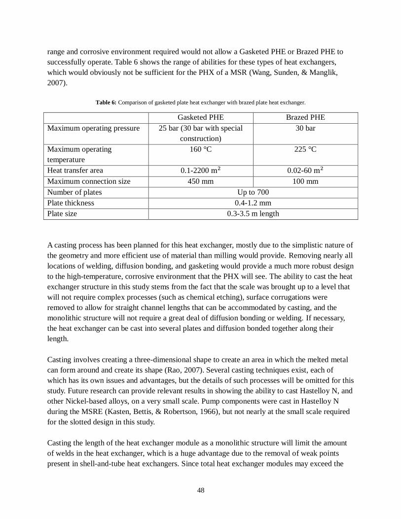
48
range and corrosive environment required would not allow a Gasketed PHE or Brazed PHE to
successfully operate. Table 6 shows the range of abilities for these types of heat exchangers,
which would obviously not be sufficient for the PHX of a MSR (Wang, Sunden, & Manglik,
2007).
Table 6: Comparison of gasketed plate heat exchanger with brazed plate heat exchanger.
Gasketed PHE Brazed PHE
Maximum operating pressure 25 bar (30 bar with special
construction)
30 bar
Maximum operating
temperature
160 °C 225 °C
Heat transfer area 0.1-2200 0.02-60
Maximum connection size 450 mm 100 mm
Number of plates Up to 700
Plate thickness 0.4-1.2 mm
Plate size 0.3-3.5 m length
A casting process has been planned for this heat exchanger, mostly due to the simplistic nature of
the geometry and more efficient use of material than milling would provide. Removing nearly all
locations of welding, diffusion bonding, and gasketing would provide a much more robust design
to the high-temperature, corrosive environment that the PHX will see. The ability to cast the heat
exchanger structure in this study stems from the fact that the scale was brought up to a level that
will not require complex processes (such as chemical etching), surface corrugations were
removed to allow for straight channel lengths that can be accommodated by casting, and the
monolithic structure will not require a great deal of diffusion bonding or welding. If necessary,
the heat exchanger can be cast into several plates and diffusion bonded together along their
length.
Casting involves creating a three-dimensional shape to create an area in which the melted metal
can form around and create its shape (Rao, 2007). Several casting techniques exist, each of
which has its own issues and advantages, but the details of such processes will be omitted for this
study. Future research can provide relevant results in showing the ability to cast Hastelloy N, and
other Nickel-based alloys, on a very small scale. Pump components were cast in Hastelloy N
during the MSRE (Kasten, Bettis, & Robertson, 1966), but not nearly at the small scale required
for the slotted design in this study.
Casting the length of the heat exchanger module as a monolithic structure will limit the amount
of welds in the heat exchanger, which is a huge advantage due to the removal of weak points
present in shell-and-tube heat exchangers. Since total heat exchanger modules may exceed the

49
size limit for a single casting procedure, diffusion bonding may be required for combining
separate heat exchanger sections along their length.
Headers are designed to be integral to exchanger sections, allowing for monolithic structures to
be cast for the entirety of the channel lengths. Common headers at the top and bottom of each
heat exchanger section will lead to main plenums for each fluid, with each gathering to one side
of the reactor, and is then directed toward an outlet pipe. The outlet pipe will be gasketed to
allow for removal when maintenance is necessary. Rather than removing the header, this allows
for the critical components that separate fuel salt from inert salt to be unaffected.
Future studies using ProCast, a commercial software package used in determining the viability of
casting procedures for geometries of interest, will ultimately determine the viability of such a
design.
Materials
Several choices exist for three materials decisions in such a heat exchanger design: heat
exchanger metal, fuel salt, and coolant salt. The studies conducted at ORNL used a wide variety
of materials for each function, but the focus of the studies was on a Hastelloy N (heat exchanger
solid), F-Li-Be- - (fuel salt), and 𝑁𝑎𝐵 -NaF (coolant salt). Explanations of each
material and the choice made for this study are shown below.
Heat Exchanger Solid
There was a relatively great deal of flexibility with the choice of HX solid, and the decision was
made based on corrosion properties, heat exchanger performance capabilities, and ease of
manufacturing. Hastelloy N, TZM (a Titanium-Zirconium-Molybdenum alloy), and pure
Molybdenum were the final three candidates. Ceramic compounds are an intriguing option for
high-temperature applications in the future, but their performance has been uninspiring thus far
(Olson, 2009). Several studies have been conducted solely on this issue, so it will not be a major
focus of this report.
Several of the solid materials offer intriguing benefits, but also come with potentially serious
flaws. All three of the candidate solids offer exceptional corrosion resistance, especially when in
contact with molten salts, but the experience with Hastelloy N provides the most appealing basis
of studies regarding creep, irradiation damage, and manufacturing experience. Pure Molybdenum
provides the best heat transfer properties, but it is known to be difficult to manufacture on the
scale required for this design. TZM is an intriguing balance between Hastelloy N and
Molybdenum, but the minor advantages it may bring in heat transfer and high-temperature

50
performance are outweighed by the vast experience Hastelloy N gained during ORNL’s research
in molten salts.
Appendix E: Material Properties
Appendix E contains a data sheet from the manufacturer of Hastelloy N, Haynes International,
which provides physical properties and approximate chemical composition of the material.
Concise documentation is available from ORNL during early studies looking into the
requirements for MSBR materials and later development of INOR-8, which came to be known as
Hastelloy N (McCoy Jr & Weir Jr, 1967).
Fuel Salt
The fuel salt is a combination of 𝐿 7 iF-𝐵𝑒 - 9
(68.5 – 31.1 – 0.2 mole %), which is rather
defined in MSBR designs and was not changed for the purposes of this study (Robertson, Smith,
Briggs, & Bettis, 1968). Polynomial expressions were available for the density, thermal
conductivity, and viscosity of the fuel salt (Cantor, Cooke, Dworkin, Robbins, Thoma, & Watson,
1968), while specific heat was assumed to be constant (as a temperature-dependent polynomial
expression is unknown).
Appendix E contains data from ORNL regarding the material properties for the fuel salt.
Coolant Salt
The secondary coolant salt options include FLiNaK, 𝑁𝑎𝐵 -NaF, FLiBe, and some inexpensive
chloride salts that could all be used to transfer heat. Coolant salts were contrasted based on
melting temperature, compatibility with Hastelloy N, cost, heat transfer characteristics, and
operational experience.
Clean FLiBe ( 𝐿 7 iF-𝐵𝑒 at 66-34 mole %) was chosen due to the wealth of knowledge and
experience associated with it, as well as its known compatibility similarities with the fuel salt and
metals. FLiBe is typically enriched in lithium-7 to enhance neutronics, but this costly procedure
may be avoided in secondary salts to provide a more cost effective solution. Cheaper options
exist for the coolant salt, but changing the composition will not affect results greatly due to the
relative similarity of all molten salts’ properties. The wealth of knowledge and experience about
FLiBe was an extremely attractive option for the secondary salt, and was weighed more heavily
than cost, which is minimal when considered relative to the scale of the entire plant (Robertson,
Smith, Briggs, & Bettis, 1968).
Polynomial expressions were available for the density, thermal conductivity, and viscosity of
FLiBe (Sohal, Sabharwall, Sharpe, & Ebner, 2010), while specific heat was assumed to be
constant (as a temperature-dependent polynomial expression is unknown).

51
Appendix E contains the fluid properties of the 𝑁𝑎𝐵 -NaF used in the MSBR design as well as
those for FLiBe used in this study.
Heat Exchanger Design
Compact heat exchangers have evolved greatly in the last several decades to become more
compact and efficient than ever. Modern materials advancements and manufacturing techniques
have allowed for dimensions to steadily decrease, resulting in designs that are increasingly more
compact and efficient. The use of circular, or semi-circular, channels has been utilized in several
modern designs with channel dimensions much less than 1mm in hydraulic diameter, with
performance that reflects the complexity of the designs. Though those dimensions are not
reasonable for the purposes of a PHX, mostly due to maintenance restrictions (channels must be
large enough to perform reasonable inspections), the concept of using smaller channels remains
an interesting concept. The degree to which the PHX dimensions can ultimately approach those
of modern compact heat exchangers will ultimately determine the viability of compact heat
exchangers in the nuclear industry.
Removing and/or altering several characteristics of recent compact heat exchangers, such as the
Printed Circuit Heat Exchanger (PCHE) designed by Heatric, can result in a heat exchanger
design suitable for use in a Molten Salt Reactor. The concepts that make the design of the heat
exchanger in this study innovative are explained in the subsequent section.
Design Changes
The two most prominent heat exchanger designs for uses in nuclear applications, albeit on the
secondary molten-salt-to-gas heat exchanger, are the PCHE (Figley, 2009) and Offset Strip-Fin
HX (Hechanova, 2007). These heat exchanger designs employ channels on the micro-scale by
using complex chemical etching and diffusion bonding processes to construct the heat exchanger.
Maintaining such designs would become very difficult as channel dimensions grow smaller and
surface features become more complex, so several aspects of these designs must be stripped
away in order to arrive at a design that can be adequately maintained.
The PCHE and Offset Strip-Fin HX each have channel diameters well below 1mm, which lead to
excellent efficiencies and can provide compactnesses of up to 2500 . Though that scale
provides several difficulties in molten-salt-related applications, the potential rewards are
significant. Fouling could easily block channels on such a small scale, and mal-distribution
effects would become even stronger in individual channels where that occurred. Loose
impediments present in any flow path in complex nuclear applications could also provide
significant detriments to performance in smaller, individual channels more so than in other

52
designs. Loose parts, solids that have plated out during operation, and other impediments are
inherently present in plants during operation, so precautions such as filters and screens must be
provided. Raising channel dimensions, namely height, to become less susceptible to blockage
can further increase robustness.
As previously described, high-frequency eddy current inspections have been used in medical
applications on circular channels of very small dimensions, but the smallest size to date was only
1.8034 mm in diameter. This provides an approximate lower limit of the channel dimensions, but
also provides an important maintenance advantage for this design. In order to push the limits of
heat exchanger performance, this dimension must be further reduced in full-scale final design
options. The development of eddy current probes of even higher frequency may be required to
meet performance requirements. Transitioning from more well-known circular cross-section
eddy current probes to pancake-style probes will also be a required design challenge.
The design presented in this report will feature high-aspect-ratio rectangular channels on the
scale of 0.5-5 mm in height, with resulting hydraulic diameters in the range of 1-5 mm. “Slotted”
channels can be limited in flow velocity to maintain laminar flow, especially when compared to
channels of circular cross-section. The lower flow velocities and increased ratio of area-to-
perimeter tend to hurt heat transfer performance and raise pressure drop, but their efficient use of
material can justify small decreases in heat transfer performance.
Recent manifestations of compact heat exchangers in nuclear applications, such as the PCHE or
Offset Strip-Fin HX, use circular or semi-circular channel cross-sections and are readily
produced by revolutionary chemical etching and diffusion bonding processes. The scale at which
they are produced limits the cross-section to these shapes, but larger channels would not require
such complex processes. A transition to a simple casting process could provide attractive
simplifications when compared to compact heat exchanger processes and economic advantages
compared to shell-and-tube processes.
In order to further simplify manufacturing to a traditional casting process, as well as to provide
more well-known maintenance options for the heat exchanger, surface corrugations and wavy
channel paths have been omitted from the design. These design options increase heat transfer
performance and limit pressure drop, but render the heat exchanger channels difficult to maintain
and produce. If maintenance techniques are proven to handle such surface features in the future,
corrugations could then be added to the design to improve its performance. Relatively simple
chevron patterns may be added if eddy current probes can follow the path down the length of the
exchanger, but preliminary designs will omit such features at the detriment of their final results.
The ultimate heat transfer performance would be seen from heat exchanger channels of
alternating composition in each direction, what can be called a “checkerboard” configuration.

53
Header designs for heat exchangers of alternating composition in each direction are prohibitively
complex and difficult to maintain. For the simplicity of header designs, each row of the heat
exchanger was kept with the same fluid. The header can then be simplified to an extension of the
channel length, with each fluid being brought together on opposing sides of the heat exchanger.
Headers can be cast, integral to the rest of the heat exchanger length, as a further means for
simplifying and streamlining the manufacturing process. Figure 15 shows a simple sketch of
such a header design, where the “hot” fluid (red) is shown flowing into the “hot” header from the
left and downward through the heat exchanger and the “cold” fluid (blue) is shown flowing
upward through the channels and out of the “cold” header to the right:
Figure 15: Slotted minichannel heat exchanger with header appearing as a continuation of the channel length.
With rows using the same fluid across their entirety, it no longer made sense to contain the fluid
region into a larger number of separate circular channels. The use of large, thin openings of
rectangular cross-section could provide an avenue to lower the amount of material used in the
design while accommodating similar usable heat transfer area. This function removes
unnecessary material between adjoining channels of similar composition, thus raising the
material efficiency (SA/MAT) without damaging heat transfer performance. The subsequent
section of this report will discuss the performance of heat exchangers utilizing channels of
circular cross-section and the “slotted” design.

54
Slotted Design
Figure 16 shows an isometric view of a 2-channel by 4-channel array used in introductory
studies for the slotted heat exchanger. The 8 channels, which act as a 4-channel by 4-channel
array (16 total channels) due to the symmetry plane shown on the right side of the drawing, will
be used in preliminary studies to compare channel dimensions and provide validation data.
Figure 16: 2-channel b 4-channel array of slotted channel used in preliminary study.
The diagram shown in Figure 16 displays the entirety of the geometric parameters for a
theoretical “slotted” heat exchanger design containing 16 channels. Channel height (H), channel
width (W), and channel length (L) were altered to determine the optimal design. The spacing
between channels, both in the height-direction (SH) and width-direction (SW), were manipulated
to provide sufficient strength. Channel dimensions were parameterized in ANSYS Workbench to
allow for easy manipulation of each of the design’s input parameters.
The channel height (H) will extend radially outward from the reactor, with the number of
channels in height,𝑁𝐻, controlling the radial dimension of the heat exchanger module as they are
connected along their length to an outer containment wall parallel to the height of the reactor.
The heat exchanger will be arranged around the reactor, with the Length (L) pointing vertically.
The heavier fuel salt will be pumped downward through half of the heat exchanger channels,
while the coolant salt will flow upward through the remaining channels. As shown in Figure 14,
the fuel salt will return to the reactor on the two cold legs of the reactor core.
Full-scale studies will use a larger array of channels but will employ a similar method of
construction. Whereas 16 channels are modeled in the preliminary studies, 45 channels will be
studied in the full-scale simulation. An array, 2.5 channels in width and 4.5 channels in height,
will be modeled as shown in Figure 17. The symmetry plane (shown in yellow) was placed in the

55
center of channels in both the width- and height-directions to allow for greater returns from the
symmetry condition.
Figure 17: Full-size channel array of 2.5 channels by 4.5 channels (hot channels shown in red, cold channel shown in blue,
symmetry plane shown in yellow, and HX material shown in black).
Compact heat exchanger channels of rectangular cross-section are not a revolutionary concept by
themselves, but finding an intermediate range of high aspect ratio rectangular minichannels in a
MSR application differs greatly from the original design. With a known concept that is expected
to provide reasonable returns in performance, a slotted heat exchanger must be modeled and
simulated to confirm its results. The subsequent several sections will lay out the process used to
model heat transfer in the slotted minichannel system.
Assumptions
Several characteristics of the design can be simplified or ignored to allow for more manageable
computations in the early stages of design.
Symmetry
The computational domain of a heat exchanger can be quartered by dividing the geometry into
four equal sections. Results can be extended to the other three sections to gain total results, but
the ability to lessen computational requirements by more than 75% is a huge advantage when
limited computing power is available. Figure 18 shows the computational domain being cut in
half by dividing the geometry into two equal halves. As long as boundary conditions and
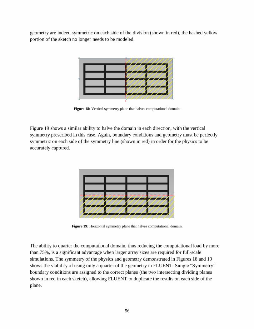
56
geometry are indeed symmetric on each side of the division (shown in red), the hashed yellow
portion of the sketch no longer needs to be modeled.
Figure 18: Vertical symmetry plane that halves computational domain.
Figure 19 shows a similar ability to halve the domain in each direction, with the vertical
symmetry prescribed in this case. Again, boundary conditions and geometry must be perfectly
symmetric on each side of the symmetry line (shown in red) in order for the physics to be
accurately captured.
Figure 19: Horizontal symmetry plane that halves computational domain.
The ability to quarter the computational domain, thus reducing the computational load by more
than 75%, is a significant advantage when larger array sizes are required for full-scale
simulations. The symmetry of the physics and geometry demonstrated in Figures 18 and 19
shows the viability of using only a quarter of the geometry in FLUENT. Simple “Symmetry”
boundary conditions are assigned to the correct planes (the two intersecting dividing planes
shown in red in each sketch), allowing FLUENT to duplicate the results on each side of the
plane.

57
Perfect Casting
The model used in this study has perfectly square channels to allow for simpler and easier
meshing. In reality, parts will come out with corners that appear more as fillets than as right
angles. The effects of such geometry changes were assumed to be negligible in this study but
should be addressed in more concise studies in the future. Figure 20 shows how a rectangular
channel would actually appear, with fillets in the corners resulting from casting, while the perfect
geometry used in FLUENT is shown on the right.
Figure 20: Actual manufactured channel (left) will differ from modeled channel (right) in applications.
Assuming the satisfaction of negligible manufacturing tolerances is generally acceptable on a
small scale but compounding the error of one channel on thousands of channels will result in
measurable changes. However, any curved edges will only improve the performance because
they will eliminate the no-heat-flux corners that hurt the performance of rectangular channels.
Corrosion/Erosion Effects Negligible
The effects of corrosion and erosion will be considered throughout the design of the heat
exchanger, but fouling effects cannot be properly modeled in FLUENT. Conservative design
ranges should be considered to allow for the increased effects of corrosion and erosion as
operation time lengthens.
Channels of insufficient dimension could be blocked by fouling, rendering them useless. Those
that could still remain in operation with corrosion effects could result in hot spots and/or uneven
wear due to the extended surface. Heat transfer performance will be hindered in all cases.
However, the model used in this research assumes that corrosion and erosion effects are
negligible. Future studies with physical test apparatuses can determine the actual changes.
Steady-state Operation
Transient conditions must be tested separately from the normal operating conditions of the heat
exchanger due to the important effects of thermal transients on compact heat exchangers. This
study, however, will focus on steady-state conditions.

58
Single-Phase Flow
Molten salts have high boiling temperatures that will not be approached in the temperature range
used in this study. FLiNaK, a common molten salt considered to be a candidate secondary
cooling salt, for example, has a boiling point of 1843 K (Sohal, Sabharwall, Sharpe, & Ebner,
2010). By maintaining temperatures below 1000 ºC, single-phase flow can be assumed through
calculations.
Outer Wall of Heat Exchanger Boundary Condition
All piping and heat exchangers must be placed in an elevated temperature inside primary
containment just outside of the reactor vessel in order to disallow the possibility of solidification
of the coolant. For these reasons, heat flux on the outer surfaces of the wall has been assumed to
be 0 in many studies (Figley, 2009). Such a boundary condition will not properly convey the
physics occurring in this application.
The construction of a Molten Salt Reactor will require assurance that the salt will never solidify
in the piping and heat exchanger. The addition of clamshell heaters surrounding every pipe and
component would be costly, cumbersome, and would bring forth significant hurdles in
maintenance operations. The MSBR planned for all necessary components to be contained in a
secondary environment raised to a temperature of 1100 °F (866.5 K) to ensure that the coolant,
blanket, and fuel salts will remain in their liquid forms even when the reactor system temperature
drops nearer their melting points (Kasten, Bettis, & Robertson, 1966).
For this study, outer walls of each heat exchanger array were assumed to be at the elevated room
temperature of 1100 °F.
Roughness Effects
For the purposes of this study, roughness along the channels was assumed to be negligible.
Casting and manufacturing processes will never present a surface that is without some minor
roughness effect, but the increased computational load required to model such an effect is not
necessary for the scope of this research. Any roughness actually present in a manufactured and
tested heat exchanger will enhance heat transfer performance.
Inlet/Outlet Effects
Headers have been neglected in the work performed in this report. For this reason, heat exchange
in the cross-flow region of the headers will be neglected. Hydrodynamic effects, such as sudden
expansion and contraction of flow area, will also be neglected in this study.

59
Composition-dependent Salt Properties
A Fluorine-Lithium-Beryllium compound composed of 𝐿𝑖 7 -𝐵𝑒 (66-34 mole %) was
developed and studied in-depth at ORNL in the 1960’s and 1970’s. The properties and behavior
of this fluid was chosen for use in the MSR, and a great deal of knowledge was developed in the
decades of its prominence. In 1967, ORNL published a report based solely on describing the
properties of FLiBe, while providing temperature-dependent correlations for each of its major
heat transfer properties (Cantor, Cooke, Dworkin, Robbins, Thoma, & Watson, 1968).
The coolant salt, assumed to be FLiBe for this study, will have a relatively similar composition
to that of the fuel salt. Comprised mostly of the same constituents as FLiBe, with trace amounts
of Uranium (U) added, the fuel salt will inherently have dissimilar properties to the clean
secondary salt. The degree to which the two liquids’ properties are different was not known, and
was studied to assure that they must be modeled as such.
Equations 1 through 4 describe the fluid properties for FLiBe (Cantor, Cooke, Dworkin, Robbins,
Thoma, & Watson, 1968):
[ ] [ ] Equation 1
[
] Equation 2
[
] Equation 3
[ ][
] Equation 4
ORNL released a document regarding the properties of several salts, with the Thorium- and
Uranium-containing fuel salt being of importance for this study in the same 1968 document
(Cantor, Cooke, Dworkin, Robbins, Thoma, & Watson, 1968). The correlations from this source
for fuel salt are laid out in Equations 5 through 8.
[ ] [ ] Equation 5

60
[
] Equation 6
[
] Equation 7
[ ][
] Equation 8
The option of assuming similar properties for the fuel and coolant salts was explored, and recent
results from Idaho National Laboratory (INL) were used after being studied extensively in 2010
(Sohal, Sabharwall, Sharpe, & Ebner, 2010). Equations 9 through 12 shows the most recent
correlations for the properties of FLiBe.
[ ] [
] Equation 9
(
[ ]) [ ] Equation 10
[
] Equation 11
[ ][
] Equation 12
The measurement techniques used in the 2010 INL experimentation are much more precise than
those used in the 1960’s when ORNL recorded the values for fuel salt. Recent studies involving
clean molten salts have increased the knowledge of those fluids, but fuel salts have been ignored
since the MSRE in the 1960’s and 1970’s. For this reason, the fluid properties for the fuel salt
given in ORNL documentation (Kasten, Bettis, & Robertson, 1966) are the only option for
contrasting against the clean salt. Table 7 has the fluid properties for fuel salt, given with
relatively large tolerances due to the limitations brought on by measuring equipment.

61
Table 7 shows a preliminary study on the FLiBe properties found in the studies in 1968, where
the composition was altered slightly to account for some discrepancies. The correlations were
applied at the anticipated average fluid temperature of 1150 °F.
Table 7: Properties of FLiBe from old study (ORNL) and recent study (INL).
Document ORNL 2316 INL – 18297
Year 1968 2010
Composition LiF-BeF2 LiF-BeF2
Composition % 66-34 67-33
𝑟 [F] 1150 1150
𝑟 [C] 621.11 621.11
𝑟 [K] 894.26 894.26 % difference
µ [Pa-s] 0.0077279 0.0077279 0
𝑝 [J/kg-K] 2386.5 2365 0.9090909
k [W/m-K] 1 1.076827 7.1345722
[kg/ ] 1953.1338 1976.77 1.195698
Table 8 shows the results comparing the best-known correlations for fuel salt at 1150 °F with the
best-known results for FLiBe at the same temperature.
Table 8: Comparison of FLiBe with fuel salt.
Document ORNL 2316
INL -
18297
Year 1970 2010
Composition LiF-BeF2-ThF4-UF4 LiF-BeF2
Composition % 73-16-10.7-0.3 67-33
𝑟 [F] 1150 1150
𝑟 [C] 621.11 621.11
𝑟 [K] 894.26 894.26 % difference
µ [Pa-s] 0.010764312 0.0077279 28.208138
𝑝 [J/kg-K] 1423.5 2365 66.139796
k [W/m-K] 1 1.076827 7.1345722
[kg/ ] 3218.07 1976.77 38.572809

62
Temperature-dependent Salt Properties
The relatively wide range of temperatures used in this study led to material properties that were
expected to vary rather significantly. A preliminary study on the temperature-dependence of
FLiBe at each end of the temperature spectrum was studied.
Table 9 shows the change in fluid properties of FLiBe across the secondary coolant’s
temperature range (850-1111 °F). Significant changes, especially in viscosity, are seen for
FLiBe.
Table 9: Properties of FLiBe over its operating range.
Document INL – 18297 INL – 18297
Year 2010 2010
Composition LiF-BeF2 LiF-BeF2
Composition % 67-33 67-33
T Minimum Maximum
𝑟 [F] 850 1111
𝑟 [C] 454.44 599.44
𝑟 [K] 727.5944 872.59 % difference
µ [Pa-s] 0.02022016 0.008577103 57.581427
𝑝 [J/kg-K] 2365 2365 0
k [W/m-K] 0.993494 1.065994 6.801164
[kg/ ] 2058.555 1987.400672 3.4565182
Just as Table 9 studies the change of the secondary coolant in its respective temperature range,
Table 10 shows the change of the fuel salt across its temperature range (1000-1300 °F). The fuel
salt’s known correlations are relatively inaccurate because of the limited measuring resources at
the time of their collection.

63
Table 10: Properties of fuel salt over its operating range.
Document ORNL 2316 ORNL 2316
Year 1970 1970
Composition
LiF-BeF2-
ThF4-UF4 LiF-BeF2-ThF4-UF4
Composition
%
73-16-10.7-
0.3 73-16-10.7-0.3
T Minimum Maximum
𝑟 [F] 1000 1300
𝑟 [C] 537.78 704.4
𝑟 [K] 810.93 977.59 % difference
µ [Pa-s] 0.007117457 0.01772438 149.02686
𝑝 [J/kg-K] 1423.5 1423.5 0
k [W/m-K] 1 1 0
[kg/ ] 3092.78 2982.79 3.5563474
The results showed that the clean FLiBe and fuel salt were quite different in their material
properties, and it was necessary that they be modeled and treated as such in FLUENT. In
addition to differentiating between fuel salt and secondary salt, the results showed that properties
varied widely over the temperature range in which they operate. For this reason, polynomial
expressions were found for each material property for later use in FLUENT.
In order to be able to use the “Polynomial” function for temperature-dependent properties in
FLUENT for the FLiBe density function, which is given as an exponential in Equation 13, the
Curve Fitting Toolbox was used in MatLab to match the exponential equation to an equal
polynomial over the same price range. With an R-value of exactly 1, the following second-order
polynomial equation is a perfect match between 800K and 1100K:
Equation 13
where is the fluid viscosity and T is the fluid temperature, measured in Kelvin. Fluid properties
varied widely in both fuel compositions and across the temperature range, so polynomial
expressions of each composition were used in FLUENT during this study. A simplification of
common materials and constant material properties would have rendered the FLUENT model
inaccurate, and adding each respective aspect of the design was not prohibitively time-
consuming.

64
These findings and decisions will play a large role in determining the viability of the CFD
simulations carried out in this research. The FLUENT design process will be laid out in the next
section of this thesis.
FLUENT Design Process
ANSYS Workbench, in conjunction with FLUENT and several built-in design modules, was
used to build, design, analyze, and optimize the design of the slotted heat exchanger in this study.
Workbench displays the steps needed throughout the process, and each module will be described
as it appears in Figure 21.
Figure 21: ANSYS Workbench interface showing FLUENT and Goal-Driven Optimization modules.
The subsequent sections will cover the theory and process followed for each step, as performed
in ANSYS Workbench.
Geometry
The first step in preparing a problem for ANSYS/FLUENT is creating and defining the cell zone
domains for later use in the problem. ANSYS DesignModeler is the geometry builder in ANSYS
Workbench that was used to construct the heat exchanger solid regions and fluid regions in this
project.

65
The model was built with the ability to parameterize each dimension for ease of change later.
Parameterizing each dimension also allowed for automated altering of dimensions, as described
later in this section.
First, the solid section of the heat exchanger was constructed in numerous individual pieces.
Each piece was selectively chosen to allow for matching nodes along the solid-fluid interface and
rectangular mesh distribution throughout the domain. As shown in a front view of the model in
Figure 22, the different colored pieces denote separate sections created in DesignModeler.
Figure 22: Full-size geometry model created in ANSYS DesignModeler with only solid regions built.
After creating the solid portion of the exchanger that surrounds the fluid in the heat exchanger,
the “Fill” function was used to fill the empty space between the solids. This creates the fluid
domain for each channel of the heat exchanger. The cross-section of the final geometry model
appears as it is shown in Figure 23 below.
Figure 23: Full-size model from ANSYS DesignModeler with fluid regions filled and highlighted.

66
ANSYS DesignModeler has the ability to parameterize all dimensions to allow for automated
manipulation later in the design process. In order to take advantage of this function, the
dimensions were entered as seen in Figures 24 and 25.
Figure 24: Isometric view of full-scale geometry with symmetry plane shown.
Figure 25: Front-view of full-scale geometry from ANSYS DesignModeler with geometric parameters shown.
Preliminary studies use geometries with 2 channels in the width-direction of similar composition
and 4 channels stacked vertically of alternating composition. Heat transfer coefficient results for
the inner channels were expected to be roughly equal to that when the heat exchanger is extended
to a larger scale, so optimization was performed on a smaller geometry to decrease run times.
The relative performance of heat exchanger channels of different sizes and lengths were first
studied on an array of channels smaller than those shown in Figures 24 and 25 in order to
decrease run times.

67
Full-scale studies must approach the actual size of a heat exchanger module using an array of 5
modules in width and 9 modules in height. Little return is seen in larger arrays, so the maximum
array size used in this study is 45 total channels (by means of a 2.5-channel x 4.5-channel
quartered model).
Mesh
Meshing is the discretization of cell zones throughout the solid and fluid domains to allow for
accurate control volume analyses (ANSYS, Inc., 2009). The process of creating a viable mesh is
influential in producing results that are accurate. Figure 26 displays the simple, structured
geometric mesh used for an initial geometry in this study.
Figure 26: Mesh created for full-scale model using ANSYS Mesher.
Due to the iterative dimensioning process used in later optimization efforts through ANSYS
Workbench, the mesh was built to be robust to changes. Edge sizing based on Element Size,
rather than Number of Elements, was used to maintain constant mesh sizing and accuracy in
larger geometries. Table 11 displays the mesh values used for all geometries.

68
Table 11: Mesh parameters used in full-scale model.
Direction X (Width) Y (Height) Z (Length)
Scale ~ 50mm ~ 10mm ~ 750mm
Sizing Type Element Size Element Size Num of Div
Dimension 1e-4 m 5e-4 m 1000 m
Bias * Figure 27 * Figure 27 None
Bias Factor 2 1.5 N/A
Figure 27 shows the biasing used to have higher mesh concentration near edges and coarser
mesh in less important central areas. This change was made to ensure that boundary layer growth
and behavior was accurately captured during its growth. The “inverse bell curve” mesh is a
method for more economically distributing mesh elements to produce similarly correct results
(Figley, 2009).
Figure 27: Mesh distribution that biases smaller nodes closer to outer walls.
Bias Factors are available in the ANSYS Mesher to account for more variations near wall
boundaries than at the center of flow regions, where changes are not as prominent. The same
number of nodes can be positioned more efficiently along each direction to better capture the
physics occurring. As seen in Table 11, Bias Factors were used on both the fluid height and fluid
width in order to capture any effects that may be seen on the boundary-layer-level in each
direction. The effects of Bias Factors can be seen in Figure 26, where mesh elements are used
more efficiently to cover the same length span.
The details and results of the parametric mesh study are shown in Appendix B.
Mesh Quality
Limitations of mesh density are not only based on the accuracy of the results rendered but also
based on several mesh statistics that describe the geometric properties of the mesh elements.
Skewness and Aspect Ratio were the two fundamental measures of mesh quality used in this
study.
Skewness measures a mesh cell’s deviation from a cell with equal sides and angles throughout its
volume. Table 12 shows the ranges in which skewness is measured, and the respective quality
for each provided by ANSYS (ANSYS, Inc., 2009):

69
Table 12: Ranges of mesh cell skewness and their respective ranges.
Value of
Skewness
Cell
Quality
1 degenerate
0.9 -- <1 bad
0.75 – 0.9 poor
0.5 – 0.75 fair
0.25 – 0.5 good
>0 – 0.25 excellent
0 equilateral
For 3-D meshes, mesh skewness values at or below 0.4 are said to be acceptable (ANSYS, Inc.,
2009). Equation 14 describes the process for finding the skewness of a cell element.
Equation 14
Aspect ratio, another key metric that describes the viability of mesh elements, describes the
relationship between the dimensions of an element in all three spatial directions. As the aspect
ratio grows larger, the element becomes less cubic, and results will deteriorate. Finding a balance
between lowering the number elements (high aspect ratio) with the optimal solution accuracy
(low aspect ratio) can be found around an aspect ratio of 3:1. Two extremes, a square with an
aspect ratio near 1:1 and a thin rectangle with an aspect ratio near 20:1, are shown in Figure 28
(ANSYS, Inc., 2009).
Figure 28: Two cells, one of high aspect ratio (left) and one of minimal aspect ratio (right).
All meshes were checked to determine that aspect ratio and skewness were kept to acceptable
levels, as prescribed in the previous several paragraphs. Special care was taken to conservatively
sacrifice mesh count, and thusly run time, in order to maintain accuracy in the results.

70
FLUENT Setup
Creating the geometry and mesh are major steps toward solving a CFD problem, but assigning
boundary conditions and other necessary characteristics can be done in the Setup module of
FLUENT within ANSYS Workbench. The important features and setup characteristics will be
explained here.
Models
Several models are available in FLUENT for applications requiring complex physical processes.
Obscure models, such as Radiation and Acoustics, were kept “Off”, as this simplistic model does
not require such capabilities. Table 13 summarizes the models used in the FLUENT model in
this study.
Table 13: Models used in FLUENT set up of full-scale simulation.
Model Status (On/Off/Other)
Multiphase Off
Energy On
Viscous Laminar
Radiation Off
Heat Exchanger Off
Species Off
Discrete Phase Off
Solidification & Melting Off
Acoustics Off
Due to compact heat exchangers nearly always being operated in the laminar regime, in order to
maintain reasonable pressure drops, preliminary studies were performed using the Laminar
model. Future studies may require improved heat transfer, so subsequent iterations of this study
may replace this with the Turbulent model.
Materials
Material property correlations were presented in the previous section of this report, and the
reasoning for providing all material decisions was also described. FLiBe was chosen as the
secondary salt, uranium-containing FLiBe was chosen as the fuel salt, and Hastelloy N was
chosen as the solid material. The temperature-dependent polynomial expressions provided for
each material in ORNL documentation, as described previously, were entered into FLUENT Set
Up.

71
Cell Zone Conditions
As FLUENT reads the mesh prepared in ANSYS Mesher, the Cell Zones conditions read in the
separate regions of solid and fluid. Due to the geometry and mesh prepared previously to
FLUENT reading the data, a separate (N) number of contiguous fluid regions are imported and
surrounded by one monolithic solid structure.
Boundary Conditions
Several boundary conditions were input at inlets, outlets, and outer surfaces to arrive at the
appropriate physics that such a heat exchanger would see in practical use. Some constraints were
given from ORNL specifications and others provided some freedom in changing parameters to
arrive at an optimal design.
Velocity inlets were prescribed at each inlet face for both fluids in all studies. As mentioned
previously, the velocity must assure laminar flow throughout the heat exchanger. The velocity
inputs for each fluid were parameterized to allow for automated manipulation in ANSYS
Workbench. Inlet temperatures were strictly kept to the values given by ORNL, where the fuel
salt entered at 1300 °F to be cooled and the secondary coolant salt entered at 850°F to be heated.
These were strict boundary conditions followed by all ORNL heat exchanger designs, so they
were used similarly in this design.
The outlet faces for each fluid region were parameterized to allow for a change from 0 gauge
pressure, which simply measures the pressure drop for a given arrangement, to higher pressures
that more accurately mirror the design conditions seen in ORNL designs. With ANSYS
Workbench able to manipulate such boundary conditions, a seamless transition from small-scale
to full-scale is possible.
In locations where fluid cell zones come into direct contact with solid cell zones, FLUENT
automatically creates an interface area called a “shadow zone” that allows for a more appropriate
boundary condition to be applied to the surface. In order to allow for conjugate heat transfer,
shadow zones allow for a “Coupled” thermal boundary condition that recognizes that no other
boundary condition must be prescribed at such a location.
On the outer surface of the solid, a constant temperature boundary condition was entered as an
“Input Parameter” that can be manipulated in ANSYS Workbench. The heat exchanger will be
kept in a heated environment outside out primary containment in order to avoid solidification of
either salt. The temperature at which the room must be maintained was succinctly described in
ORNL paperwork as 1100°F. Higher temperatures lead to more power spent heating the room,
but changing the outer surface temperature could provide an intriguing change to the physics that
may lead to improved performance. Future studies could inclusion more in-depth focus on
changing the outer wall temperature, as thin arrays of heat exchanger banks could provide an
easier means for avoiding solidification of the salts.

72
As explained previously in the Assumptions section of this report, symmetry boundary
conditions were placed at several locations to allow for only a fraction of the computational load
to accurately model the physics of the system. Lessening the number of cells will make runs
much more manageable
The remaining interior walls and surfaces do not require any boundary conditions to accurately
capture the heat transfer and hydrodynamics processes occurring in the flow channels.
Solution
Once properly set up and initialized, the discretized domains can be solved for the appropriate
governing equations to provide velocity, pressure, and temperature profiles. With those results
known, heat transfer and hydrodynamic properties can be extracted as needed.
FLUENT goes about solving fluid flow by discretizing the domain into separate control volumes
(Meshing, as described above), integrating governing equations over each control volume to
build algebraic equations for each variable, and linearizing these equations to yield updated
results throughout the domain.
The “SIMPLE” Pressure-Velocity Coupling Solution Method in FLUENT, which was employed
in solutions for this study, uses a segregated algorithm for solving momentum and continuity.
Figure 29 shows a schematic of how pressure and velocity are calculated using the segregated
algorithm (ANSYS, Inc., 2009).
Figure 29: Pressure-based solver used in FLUENT.

73
FLUENT solves the continuity equation, to a convergence level of 1e-4, as shown in Equation
15.
t Sm Equation 15
where , the mass added via liquid changing phase, will be zero for the simulations performed
in this study. For both the pressure-based (used in this paper) and density-based solvers
employed by FLUENT, the velocity field is solved directly by the momentum equation.
Pressure fields, on the other hand, are found by manipulating the continuity equations and
momentum equations to find a suitable solution. Pressure can be solved directly, or by means of
a pressure correction equation.
Conservation of momentum is also solved, to a convergence level of 1e-6, as shown in Equation
16.
t Equation 16
where is the stress tensor, 𝑔 is the gravitational force, and is body forces. The energy
equation is solved using the velocity and pressure profiles described previously, along with
several parameters required to be input. Equation 17 shows the process by which the energy
equation is solved in FLUENT.
( ) ( ) Equation 17
where is the effective thermal conductivity, is volumetric heat source term, E is mass-
averaged energy, and T is mass-averaged temperature.
Results
CFDPost is used to view and analyze the results from FLUENT found in the previous steps. In
addition to the powerful tools it contains for displaying data and distributions, CFDPost has the
ability to create functions and expressions for more in-depth calculations. The program was used
to create output functions for later use.

74
Automating the calculation of such important parameters simplifies the design process and
allows for those values to be used later in the process during Goal-Driven Optimization to drive
an optimal design.
Contours were viewed to confirm proper physics were being captured in FLUENT simulations.
Figure 30 shows the temperature profile at the center of a row of hot fluid channels with a
uniform inlet temperature of 977K and outlet temperatures are significantly lower.
Figure 30: Temperature contour of a hot channel produced from FLUENT.
As expected, temperature gradually changes from the prescribed input value to its final value at
the channel outlet. Additional cooling is seen at solid sections that separate flow channels and act
as fins to assist in cooling. Thermal boundary layer effects can be seen from the temperature
profile as well.
Figure 31 shows the temperature profile developing along the length of a cold channel, where the
uniform inlet temperature is shown at 727 K. The same pattern is seen in the cold channel as was
seen in the hot channel in Figure 30.

75
Figure 31: Temperature contour of cold channel produced by FLUENT.
The velocity profiles for each fluid channel are expected to approach zero at their boundaries and
their maximum at the center of each channel. Figure 32 shows the velocity profiles found in the
full-scale simulation, which performed as expected.
Figure 32: Velocity profile found from FLUENT.
Figure 33 is a temperature profile of the full-scale simulation at half of the total channel length
(Z=0.375 m). The outer channels are shown to be heated by the outer walls, which are held at
866 K, while the inner channels are transferring heat more efficiently amongst each other.

76
Figure 33: Temperature profile at half channel length shown in CFD Post.
The temperature profile shown in Figure 33 verifies the effect the outer channels felt from the
outer wall’s constant temperature boundary condition. With temperatures showing lesser effects
from transferring heat with the outer boundary seen in inner channels, the performance of those
channels is analyzed more heavily in attempts to bring the simulation to the necessary scale for a
nuclear power plant.
Additional contours are provided in Appendix G.
Parameter Set
Several parameters were varied in studies to arrive at an optimal solution. The input parameters
are shown and become available for manual or automated manipulation in the Parameter Set.
This set of parameters, along with the output parameters produced by each module, in connected
to each function in ANSYS Workbench as shown in Figure 21.
Geometric inputs from ANSYS DesignModeler are combined with input/output conditions in
FLUENT and problem specifications to create the entire list of input parameters in this study as
shown in Table 14.
Table 14: Inlet conditions provided through FLUENT for simulations.
Geometric
Inputs
H, W, HH, HW, L, SH, SW
FLUENT
Inputs
Vhot, in , Vcold, in , Toutside , Thot, in ,
Tcold, in , Phot, out , Pcold, out
Problem
Specifications
Q
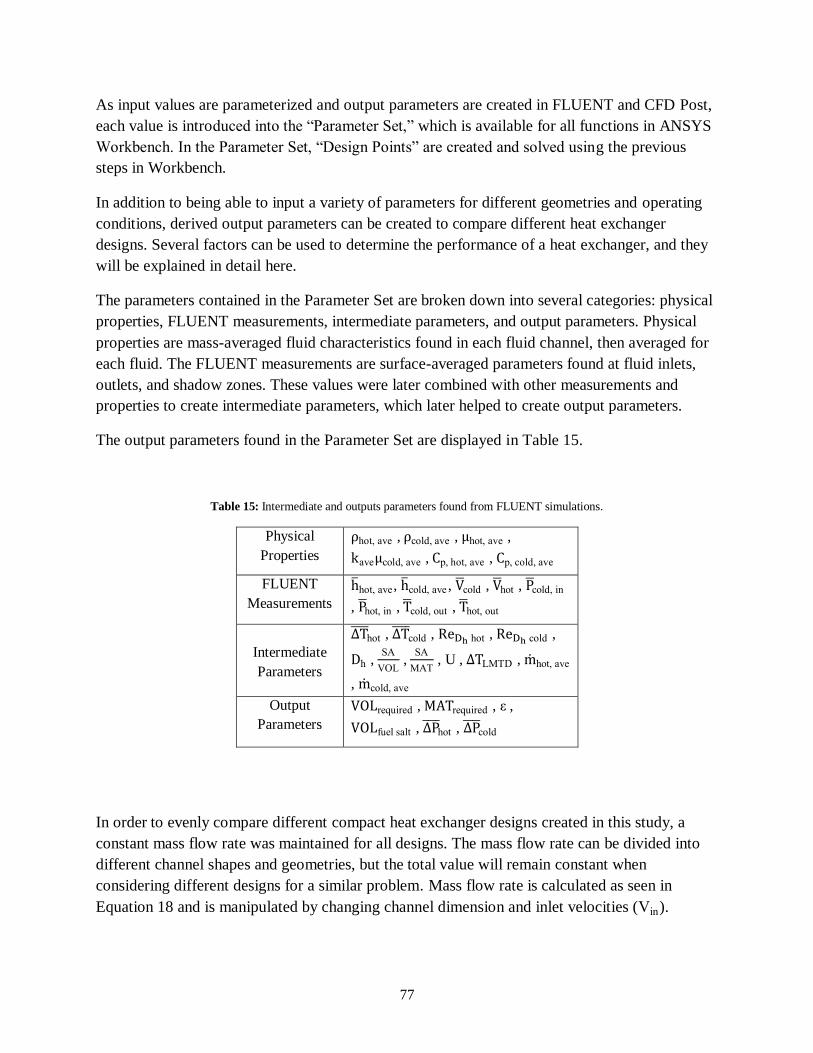
77
As input values are parameterized and output parameters are created in FLUENT and CFD Post,
each value is introduced into the “Parameter Set,” which is available for all functions in ANSYS
Workbench. In the Parameter Set, “Design Points” are created and solved using the previous
steps in Workbench.
In addition to being able to input a variety of parameters for different geometries and operating
conditions, derived output parameters can be created to compare different heat exchanger
designs. Several factors can be used to determine the performance of a heat exchanger, and they
will be explained in detail here.
The parameters contained in the Parameter Set are broken down into several categories: physical
properties, FLUENT measurements, intermediate parameters, and output parameters. Physical
properties are mass-averaged fluid characteristics found in each fluid channel, then averaged for
each fluid. The FLUENT measurements are surface-averaged parameters found at fluid inlets,
outlets, and shadow zones. These values were later combined with other measurements and
properties to create intermediate parameters, which later helped to create output parameters.
The output parameters found in the Parameter Set are displayed in Table 15.
Table 15: Intermediate and outputs parameters found from FLUENT simulations.
Physical
Properties
hot, ave , cold, ave , hot, ave ,
ave cold, ave , p, hot, ave , p, cold, ave
FLUENT
Measurements
hot, ave, cold, ave , cold , hot , cold, in
, hot, in , cold, out , hot, out
Intermediate
Parameters
hot , cold , hot , cold
,
h , SA
VOL ,
SA
MAT , U , LMTD , hot, ave
, cold, ave
Output
Parameters
required , required , ε ,
fuel salt , hot , cold
In order to evenly compare different compact heat exchanger designs created in this study, a
constant mass flow rate was maintained for all designs. The mass flow rate can be divided into
different channel shapes and geometries, but the total value will remain constant when
considering different designs for a similar problem. Mass flow rate is calculated as seen in
Equation 18 and is manipulated by changing channel dimension and inlet velocities (Vin).

78
m V Equation 18
where is fluid density, is the cross-sectional area of the flow, and V is the fluid velocity.
The flow rate relates to the amount and speed of heat that needs to be removed from the
incoming flow.
Equation 19 shows an important parameter, the hydraulic diameter, which is vital in calculating
several hydrodynamic characteristics of a flow pattern. The hydraulic diameter is vital in
developing a representative geometric “diameter” for non-circular cross-sectional areas.
Equation 19
where is the cross-sectional area of the flow and P is the wetted perimeter of the flow
channel. The hydraulic diameter of flow in a circular cross-section is simply equal to the
diameter of the channel.
Hydraulic diameter is one factor in determining the Reynolds number, 𝑒 h, a dimensionless
factor that describes the turbulence of flow. Equation 20 describes the Reynolds number, which
was closely monitored throughout testing.
Equation 20
where is the fluid density, V is the fluid velocity, is the hydraulic diameter, and is the
fluid viscosity. Reynolds number was monitored for each design to maintain a value below the
laminar-turbulent transition value. The exact laminar-turbulent transition value is not well-
known, and is often a basis for disagreement among those who have investigated it, but a simple
linear interpolation between two lesser-disputed data points was offered as a means for
determining the value over a large range of rectangular channel cross-sections (Kandlikar,
Garimella, Li, Colin, & King, 2006).
The transitional Reynolds number, 𝑒𝑡, for a square channel (aspect ratio = 1) has been found
to be 2200. For parallel plates ( = 0), the transitional Reynolds number has been shown to be
2500 (Kandlikar, Garimella, Li, Colin, & King, 2006). For any value between these two points, a
simple linear interpolation was completed. A full explanation of the laminar-turbulent transition
is provided in several texts (Kandlikar, Garimella, Li, Colin, & King, 2006). The physics behind
transitional flow is still not fully known at this point, and is not expected to play a vital role in

79
this study. A brief discussion, along with the correlation used for rectangular channels used in
this study, will be presented in Appendix F.
A number of other output parameters can be calculated by combining outputs from FLUENT to
create meaningful comparative measures. One such measure is heat exchanger effectiveness, ε,
which describes how completely heat is transferred from one fluid to the other (Kays & London,
1984), is shown in Equation 21.
( )
( ) ( )
( )
( ) ( )
Equation 21
where is the mass flow rate of the fluid, 𝑝 is the specific heat of the fluid, and T is the
temperature of the fluid. Compact heat exchangers can achieve effectiveness of up to 0.99, which
stems from the very close approach temperatures achieved by such designs (Wang, Sunden, &
Manglik, 2007).
Preliminary computations in this study compare heat exchanger channels of both circular and
slotted designs, so the following two computations will introduce geometric calculations for each
cross-section.
Another key measure in this study is compactness, or the surface-area-to-volume ratio for a
given arrangement. Compactness offers perspective on the ability of a given design to contain a
large amount of usable contact surface area for heat transfer in a given three-dimensional
volume. The importance of compactness, which is given for a slotted design in Equation 22 and a
circular design in Equation 23 will be explained later in this report.
(
)
[ ][ ] Equation 22
where W is width of a slotted channel, H is the height of a slotted channel, SW is the spacing
width between channels, SH is the spacing height between channels, 𝑁𝑊 is the number of
channels wide, and 𝑁𝐻 is the number of channels in height.
(
)
[ ][ ] Equation 23

80
where is the diameter of a circular channel, SW is the spacing width between channels, SH is
the spacing height between channels, 𝑁𝑊 is the number of channels wide, and 𝑁𝐻 is the number
of channels in height.
Another vital measure of the performance of a heat exchanger is the ratio of surface-area-to-
material-volume. When using materials that are as expensive as Hastelloy N, limiting the amount
of material used is a vital consideration in the final design. The relative importance of
maximizing SA/MAT will be explained in detail later in this report. Equations 24 shows the
manner in which SA/MAT can be solved for slotted designs, respectively.
(
)
Equation 24
where VOL is the volume of the given arrangement, L is the channel length, H is the slotted
channel height, W is the slotted channel width, 𝑁𝑊 is the number of channels wide, and 𝑁𝐻 is the
number of channels in height. Equation 25
(
)
-
Equation 25
where VOL is the volume of the given arrangement, L is the channel length, D is the diameter of
a circular channel, 𝑁𝑊 is the number of channels wide, and 𝑁𝐻 is the number of channels in
height. The total amount of heat removed from a heat exchanger can be found by using Equation
26.
Equation 26
where A is the surface area on which heat transfer can occur, U is the overall heat transfer
coefficient, and is the log-mean temperature difference that is defined in Equation 27
(Kays & London, 1984).
(
) Equation 27
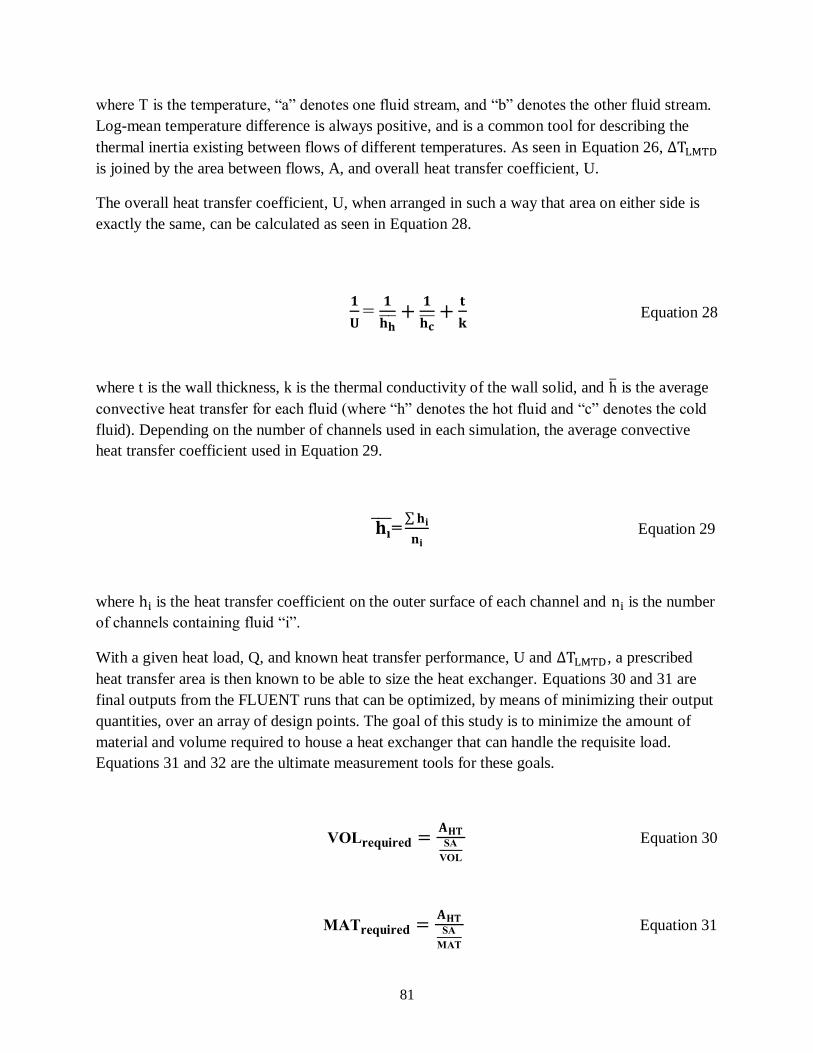
81
where T is the temperature, “a” denotes one fluid stream, and “b” denotes the other fluid stream.
Log-mean temperature difference is always positive, and is a common tool for describing the
thermal inertia existing between flows of different temperatures. As seen in Equation 26,
is joined by the area between flows, A, and overall heat transfer coefficient, U.
The overall heat transfer coefficient, U, when arranged in such a way that area on either side is
exactly the same, can be calculated as seen in Equation 28.
Equation 28
where t is the wall thickness, k is the thermal conductivity of the wall solid, and h is the average
convective heat transfer for each fluid (where “h” denotes the hot fluid and “c” denotes the cold
fluid). Depending on the number of channels used in each simulation, the average convective
heat transfer coefficient used in Equation 29.
∑
Equation 29
where is the heat transfer coefficient on the outer surface of each channel and is the number
of channels containing fluid “i”.
With a given heat load, Q, and known heat transfer performance, U and , a prescribed
heat transfer area is then known to be able to size the heat exchanger. Equations 30 and 31 are
final outputs from the FLUENT runs that can be optimized, by means of minimizing their output
quantities, over an array of design points. The goal of this study is to minimize the amount of
material and volume required to house a heat exchanger that can handle the requisite load.
Equations 31 and 32 are the ultimate measurement tools for these goals.
Equation 30
Equation 31

82
where A is the surface area required to remove the heat load with the given heat transfer
characteristics, SA/VOL is the compactness for the given setup, and SA/MAT is the
corresponding material efficiency. These results can then be compared to approximations made
from ORNL design paperwork to compare to that of their shell-and-tube design.
Another vital metric for comparing heat exchanger designs is the volume of the fuel salt required
to transfer the requisite amount of heat. As found in Equation 32 shows the process for
determining the fuel salt volume, which is found by calculating the volume of one channel and
multiplying by the number of fuel channels.
Equation 32
where H is the slotted channel height, W is the slotted channel width, L is the channel length, W
is the number of channels in width, and H is the number of channels in height. The fuel salt
volume directly affects the fissile inventory in a Molten Salt Reactor, so reducing the fuel salt
volume can lead to substantial reductions in cost for each plant startup. Transferring heat more
efficiently and effectively through a compact heat exchanger can provide significantly lower fuel
salt volumes, which will be shown later in this report.
The results found from these equations were automatically updated in the Parameter Set and
were later used in conjunction with Goal Driven Optimization (GDO) to find a final design for
this project.
Optimization
ANSYS Workbench allows for Goal-Driven Optimization that can assess several goals and
objectives in an automated manner. The steps in this process include: Design of Experiments and
Goal-Driven Optimization. They will be described in this section.
Design of Experiments (DOE)
Design of Experiments (DOE) is a function of ANSYS Workbench that allows for automated
sampling of input parameters over their entire possible range. Instead of manually altering each
problem input and combining it with every possible combination of each other input parameter,
DOE automatically completes this task and solves each Design Point in series.
Several options are available for sampling the entire possible range of input values, with options
built into DOE to most efficiently sample the space. The “Central Composite Design” method

83
with Central Composite Design was used to optimally fill the sample space (ANSYS, Inc.,
2009).
DOE creates a series of data points that cover the entire possible range of each input parameter,
which allows for a thorough understanding of the sample space at hand. With the wealth of
knowledge from the data points created and solved in DOE, a Response Surface can be built to
characterize the impact of each input parameter on each output parameter.
Optimization
A brief optimization was performed for several channel parameters to reach full designs that met
the boundary conditions prescribed in ORNL’s design. Future studies can perform more in-depth
optimization by using the Goal-Driven Optimization (GDO) module within ANSYS Workbench,
but the present study serves to offer possible design points that may be acceptable for a complete
design.
Several channel geometries and corresponding boundary conditions were altered in order to
reach the necessary target output values and parameters. The relative importance of each target
or objective can be defined independently (ANSYS, Inc., 2009). Table 16 shows the GDO goals,
limits, and priorities used for this study.
Table 16: Input and output parameters found in this study.
Parameter Optimization Goal - Priority
Level
Inputs
H 0.4 < H < 5mm
W 4 < W < 50mm
SH 0.8 < SH < 2mm
SW 0.4 < SW < 2mm
𝑃𝑜𝑢𝑡 0
𝑉𝑖𝑛 Maintain Re < 2000
Q 528.5MW
Intermediate
Values
SA/VOL --
SA/MAT --
U --
𝐿𝑀𝑇 Target – 255K
A
Outputs
𝑉𝑂𝐿𝑟 𝑞𝑢𝑖𝑟 𝑑 Minimize – High Priority
𝑀 𝑟 𝑞𝑢𝑖𝑟 𝑑 Minimize – Medium Priority
𝑉𝑂𝐿 𝑢 𝑙𝑠𝑎𝑙𝑡 Minimize – High Priority
ε Maximize – Medium Priority
𝑃 ~ ORNL value – Low Priority

84
The results of the GDO module will be presented in the subsequent section of this report as
results are reached for a full-scale design.
Results and Discussion
Three different studies were performed: model validation, small-scale comparison of channel
geometry, and full-scale comparison. The model validation step consists of comparing the results
from FLUENT to known correlations produced from other studies on rectangular channels. The
small-scale comparison looks at the performance of a circular cross-section channel and slotted
cross-section channels that were modeled in the first study. The third study seeks to build a
model that can be extrapolated to a full-scale design that can evenly be compared with ORNL’s
shell-and-tube PHX.
The results for both studies are shown below.
Model Validation Theory
The physics involved in heat transfer and fluid flow are relatively well known for rectangular
channels, so a preliminary study was launched to validate the FLUENT code and process used in
this study for such a shape. After creating a single rectangular channel, several more rectangular
geometries could then be compared to correlations that have been developed for varying channel
aspect ratios. From this point, a simple change of geometry and boundary conditions will allow
for full-scale results to be simulated and compared to ORNL’s design to test the validity of the
slotted concept.
The hydrodynamic entry length, 𝐿𝐻, must first be calculated to determine which correlation,
developing or fully-developed, should be used for calculations. Velocity profiles develop along
any surface as shown in Figure 34, where flow velocities are 0 at the wall (assuming no-slip
along the wall) and approach their nominal value once they reach the boundary layer thickness.
Figure 34: Boundary layer growth over a flat plate.
Flow becomes hydrodynamically fully developed in channel flow when the viscous boundary
layers growing from each opposing wall meet in the center of the channel. Figure 35 shows two

85
viscous boundary layers emerging from opposite sides of a channel, meeting at the center, and
becoming fully-developed as shown in the figure.
Figure 35: Boundary layer growth in channel flow.
When flow becomes fully developed, velocity profiles will no longer change until some type of
perturbation causes the boundary layers to separate and once again begin to form. A common equation for
determining the hydrodynamic entry length is found in Equation 33 (Kandlikar, Garimella, Li, Colin, &
King, 2006).
Equation 33
For a hydraulic diameter of 1mm and Reynolds number of 1000, as they are expected to be
within the typical range of values in this study, H would be only 50 mm. With values in this
range, it would be reasonable to assume that a 750 mm channel length would be fully developed
through the entirety of its length.
The property of importance in validation of the hydrodynamic testing in this study is pressure
drop, which can be found easily in CFD simulations. Equation 34 shows the four effects that
combine to form pressure drops in typical heat exchangers (Wang, Sunden, & Manglik, 2007).
∑ Equation 34
where is the pressure drop due to friction, is the pressure drop or head due to gravity,
is the pressure drop related to flow acceleration within the flow channels, and ∑ 𝑃𝑁𝑖 is the sum
of pressure drops caused by inlet and outlets. For the models produced and studied in this
research, flow acceleration and inlet/outlet conditions are neglected in straight channel sections.

86
For the preliminary study, gravity has been omitted as a means to isolate the contribution from
frictional effects, which can be readily compared to Poiseuille correlations.
Two terms combine to determine the overall pressure drop incurred in a heat exchanger channel.
Equation 35 shows the contribution from gravity, which can act to increase pressure drop (when
positive) or provide a static head (when negative) (Wang, Sunden, & Manglik, 2007).
Equation 35
The process for determining the frictional contribution to pressure drop is less direct, and
requires finding the friction factor, f, which usually involves experimental results or correlations
from previous experiments. Equation 36 shows the process by which results for frictional
pressure drop, which will dominate the contributions for the purposes of this study, are found
(Wang, Sunden, & Manglik, 2007).
Equation 36
where G is the mass flux, f is the friction factor, and L is the channel length. In order to simplify
the multitude of velocity boundary conditions that may apply to different applications, the
dimensionless Poiseuille number was determined for fully developed laminar flow and is shown
in Equation 37 (Kandlikar, Garimella, Li, Colin, & King, 2006).
Equation 37
where f is the friction factor and Re is the Reynolds number of the flow. The Poiseuille number
remains constant for channels of each cross-section and provides a valuable source for finding
the friction factor required in Equation 36 for different incoming fluid velocities.
Equation 36 can be combined with Equation 37 to relate the pressure drop directly to flow
characteristics and parameters, which will be used to show the empirical Poiseuille results later
in this study.
Equation 38

87
More in-depth studies have been completed on rectangular channels of varying aspect ratio
(height-to-width or vice versa), (Kandlikar, Garimella, Li, Colin, & King, 2006). Equation 39
shows empirical results for the Poiseuille number in fully developed flow in rectangular channels
of varying aspect ratio, .
[
] Equation 39
More exact results can be determined when removing the fully developed assumption throughout
the pipe (where the Poiseuille correlation can then be used) and solving pressure drop separately
in two distinct regions: the developing region and the fully developed region. The apparent
friction factor, 𝑓 pp, can be used in developing laminar flow as shown in Equation 40 (Kandlikar,
Garimella, Li, Colin, & King, 2006).
Equation 40
where x is the distance from the inlet to the points of interest, usually where flow becomes fully
developed, and is the mean fluid velocity. The apparent friction factor acts as an average
friction factor over the developing range, and can then be added to the fully developed pressure
drop as it occurs over the remaining channel length. A measure of the difference incurred from
using the apparent friction factor in place of the fully-developed results is captured in the
incremental pressure defect, K(x) (Kandlikar, Garimella, Li, Colin, & King, 2006). Equation 41
shows the process for finding K(x), which can be used later to show the pressure drop across
both the developing and fully-developed regions.
Equation 41
The results from Equation 41 can be combined to segregate the pressure drop results from the
developing region (using the incremental pressure defect) and the fully-developed region (using
the Poiseuille number) to form Equation 42, which displays the full results for pressure drop.
Equation 42

88
The friction factor is heavily dependent on empirical results, and robust correlations have been
developed for channels of different cross-section and boundary condition to cover a wide range
of applications. Figure 36 shows a known range of correlations for Po as a function of channel
aspect ratio (shorter channel height/longer channel width) (Kays & London, 1984) assuming
fully developed flow in the rectangular channel.
Figure 36: Poiseuille correlation for varying rectangular channel aspect ratio (Kays & London, 1984).
Hydrodynamic effects can be equally compared to the results seen in Figure 36 for fully
developed flow, but the heat transfer (and corresponding thermal development region) cannot
use the same assumption.
Thermal entry length calculations are performed in a similar manner to that of the hydrodynamic
development, which was explained previously. Analogous to Figure 35 above for hydrodynamic
flow development, channel flow becomes thermally developed once its thermal boundary layers
meet in the center of the pipe. Figure 37 shows both the hydrodynamic and thermal boundary
layers of a channel flow for a fluid with a Prandtl number, a measure of the diffusivity of
momentum relative to heat, greater than 1 (a Prandtl number higher than 1 means that
momentum is diffused more easily than temperature, which leads to thermal boundary layer
becoming fully developed after the thermal boundary layer).

89
Figure 37: Thermally-developing channel flow for high-Prandtl number fluid.
Equation 43 shows the thermal entry length for fully developed laminar fluid flow in a
rectangular channel (Kandlikar, Garimella, Li, Colin, & King, 2006).
Equation 43
where C is 0.05 for circular channels and 0.1 for rectangular channels, Re is the Reynolds
number of the flow and Pr is the Prandtl number of the fluid (Kandlikar, Garimella, Li, Colin, &
King, 2006).
The preliminary study will be tested with mass-averaged flow velocities of approximately 1m/s
and hydraulic diameters of less than 1mm over the 0.5 m length scale. The small-scale model
used in the validation study will become fully developed at a distance of approximately 500 mm,
which is almost identical to the channel length being tested in the preliminary study. Full-scale
models will have even longer thermal development regions, so the same thermally developing
correlations will hold true in those studies as well.
Whereas hydrodynamic validation is performed by finding the dimensionless Poiseuille number,
which can be related directly to pressure drop, thermal validation is performed using the Nusselt
number. The Nusselt number compares the contributions of convective and conductive heat
transfer and is known to vary with changing channel cross-section and boundary conditions
selection, while remaining constant in fully developed flow. The Nusselt number is found
according to Equation 44.
Equation 44
where h is the heat transfer coefficient, k is the thermal conductivity, and L is the characteristic
length in the direction in which the thermal boundary layer growth of interest occurs.

90
In this research, thermal boundary layers form along the length axis and the width axis and will
reach fully developed flow once they each grow to be half the height of the channel’s cross-
section. Both the Reynolds number and Nusselt number will be calculated based on the hydraulic
diameter in this study.
Difficulties arise in producing accurate Nusselt correlations due to the sensitivity of heat transfer
to the boundary conditions used in each problem set up. Correlations have been produced for
four-sided heating (heat flux is occurring from the every outer surface of the channel) and three-
sided heating (one side is kept adiabatic, while the other three transfer heat) in developing flow
situations. Steady-state flow Nusselt correlations can use constant wall temperature, constant
heat flux (both axially and circumferentially), or uniform axial heat flux and constant
circumferential wall temperature (Kandlikar, Garimella, Li, Colin, & King, 2006).
The boundary conditions for any problem will most likely be a combination of the above-
mentioned boundary conditions and adding a different and larger array of channels will add yet
another factor to change results. For this reason, a simple study of one channel should be
sufficient to validate the process used in this study. The characteristics used in correctly finding
those results can then be expanded to a larger geometry, which can find the results for the
geometry and boundary condition at hand in this study. The Nusselt correlation found from those
results can then be presented for the specifics used in this research.
The process by which the full-scale model’s Nusselt number is found must start again at
determining the regime in which the thermal boundary layer growth will render the flow.
For channel hydraulic diameters on the order of 1 mm, Reynolds numbers maintained at
approximately 1000, and Prandtl numbers typically being 15, the thermal entry length in this
study can be found to be 1.5m by using Equation 43 Flow over the 0.75 m length used in this
study can then be assumed to be developing for the entirety of the channel length in each design
that will be tested. Such an assumption will require the use of correlations for thermally
developing flow, which differ from the fully developed flow correlations.
Thermally developing flow will have Nusselt correlations depending on channel aspect ratio, ,
and non-dimensional thermal length, Equation 45 shows the process by which this length is
found.
Equation 45
where x is the distance along the length of the channel and Pr is the Prandtl number of the fluid.
With a channel aspect ratio prescribed and characteristics of the flow and fluid known, Nusselt
correlations are tabulated as listed in Table 17 (Kandlikar, Garimella, Li, Colin, & King, 2006).

91
Table 17: Nusselt correlations for varying channel aspect ratio and non-dimensional length (Kandlikar, Garimella, Li, Colin, &
King, 2006).
≤ * = 0.25 = 0.333 = 0.5 = 1 ≥ 10**
0.0001 31.4 26.7 27.0 23.7 25.2 31.6
0.0025 11.9 10.4 9.9 9.2 8.9 11.2
0.005 10 8.44 8.02 7.46 7.1 9.0
0.00556 9.8 8.18 7.76 7.23 6.86 8.8
0.00625 9.5 7.92 7.5 6.96 6.6 8.5
0.00714 9.3 7.63 7.22 6.68 6.32 8.2
0.00833 9.1 7.32 6.92 6.37 6.02 7.9
0.01 8.8 7 6.57 6.05 5.69 7.49
0.0125 8.6 6.63 6.21 5.7 5.33 7.2
0.0167 8.5 6.26 5.82 5.28 4.91 6.7
0.025 8.4 5.87 5.39 4.84 4.45 6.2
0.033 8.3 5.77 5.17 4.61 4.18 5.9
0.05 8.25 5.62 5.00 4.38 3.91 5.55
0.1 8.24 5.45 4.85 4.22 3.71 5.4
1 8.23 5.35 4.77 4.11 3.6 5.38
* - simplified to parallel plates, both sides heated ** - simplified to parallel plates, one side heated
Results from this table can be linearly interpolated to arrive at solutions for x values at
intermediate channel aspect ratios. This empirical method of creating a correlation for this wide
variety of channel geometries and flow characteristics is seen as the most viable method in
thermally developing flows. Whereas this entire chart was developed for flow in three-sided or
four-sided heating environments, a similar chart will be developed for the intermediate situation
found in the constant outer wall temperature boundary conditions used in this study.
The results provided from the micro-scale studies previously produced are shown in Figure 38 as
a function of inverse dimensionless length. It is shown that Nusselt number decreases steadily
with an increased dimensionless length, x*, until the flow becomes thermally fully-developed
(x*=1) as shown in Figure 37, where interpolated results from Table 17 for = 0.317 are
shown.

92
Figure 38: Theoretical Nusselt number as a function of the inverse of dimensionless length (Kandlikar, Garimella, Li, Colin, &
King, 2006).
It is also useful to compare results from a more concisely presented study to validate the data
found in this study. The information found in Table 17 and Figure 38 will be useful in comparing
final results as a check for general agreement, but more concisely explained studies are available
for small-scale validation.
A rectangular micro-scale study performed by Bhanja to validate Nusselt correlations was
repeated and altered slightly to attain validation for the process and mesh used in this study
(Bhanja, 2009). Banja’s study provides a concise process for creating the geometry and boundary
conditions for a constant heat flux problem set up that was solved in the study.
A microchannel of 57 µm in height and 180 µm in width was tested over a 10 mm length
From this study, results were first matched to a study that modeled only one channel with
constant heat flux on the channel periphery and had its set up readily available (Bhanja, 2009).
Varying the channel inlet flow rate (and velocity) for a constant-size rectangular channel will
produce a correlation relating Nusselt number and Reynolds number. Reproducing these results
over a range of velocities and heat flux values will assure that the correlation is correct.
Figure 39 shows the Nusselt correlation as a function of Reynolds number provided for the
constant heat flux case modeled by Bhanja, which can be compared for a similar problem set up
prepared in this study.

93
Figure 39
The set up was matched to attempt to produce similar results to validate the methods performed
in this study. With a slightly different mesh and set up, simulations must be performed to assure
that the physics within the model at hand are accurately captured. The results of this step, as well
as the hydrodynamic validation, are shown below.
Model Validation Results
For the purposes of validation needed for the CFD model created and utilized in this study, the
results for slotted channels were compared to the correlations presented previously in this
section. In addition to providing assurance that they physics have been appropriately captured,
the mesh parameters and solution methods used can be confirmed as satisfactory for extension to
larger geometries.
A wide range of channel dimensions and inlet velocities were tested to assure agreement with
well known correlations. Equation 36 was used to find the Poiseuille number from pressure
drops found in FLUENT. Figure 40 shows the results for the Poiseuille number obtained from
FLUENT in this study, as well as a known Poiseuille correlation for rectangular channels (Kays
& London, 1984).

94
Figure 40: Poiseuille correlation results found in FLUENT validation.
These results show a general agreement in both value and trend with the known values produced
in previous studies. Percent error is kept below five percent at all data points, and a polynomial
fit was developed that nearly provides an exact match for the correlations produced from the
studies performed by Kays and London.
Figure 41 shows the results found in this study and compares them to those found in a previous
study of rectangular channels (Bhanja, 2009).
Figure 41: Nusselt correlation for varying Reynolds number in micro-scale rectangular channel (Bhanja, 2009).
With these results, the theory and mesh have shown to provide results roughly equal to those
produced by previous studies. The model and set up can then be updated to include a larger
95
geometry and slightly different boundary conditions to simulate small-scale rectangular
minichannels, as well as a relatively large array of full-scale channels.
Comparison of Circular and Slotted Designs
The first step in moving from modern compact heat exchangers to a slotted design is to compare
the performance of a slotted heat exchanger to that of the more traditional circular cross-section
channels. Due to eddy current inspections being further developed in circular cross-sections than
high aspect ratio slotted designs, it may be an advantage to stay with circular channels. All
designs were kept with constant total mass flow rates and equal hydraulic diameters in an
attempt to produce similar Reynolds number and pressure drop values. Slotted designs of high
aspect ratio (W/H) and low aspect ratio were tested.
With a channel diameter of 1 mm determined for the circular channels, the high apsect ratio
slotted channel arrangement was brought to channel widths of 11.56 mm and channels heights of
0.5225 mm to arrive at the same hydraulic diameter (1 mm) while keeping a channel aspect ratio
in excess of 10 for the slotted design. The low aspect ratio channel arrangement has a channel
height of 0.75 mm and a width of 1.5 mm, arriving at the same hydraulic diameter of 1mm.
Maintaining similar hydraulic diameters for different channel geometries is important due to the
need to compare the overall perfromances designs can offer while providing similar pressure
drops. As a slotted channel is increased in channel width (W), thus becoming thinner and more
infinite in aspect ratio, SA/VOL and SA/MAT values will become increasingly better. As the
geometric properties are improved by thinning and widening the channel, hydraulic diameter
increases to limit the velocity of the fluid to maintain laminar flow, adversely affecting
performance. Finding the optimal balance between these two effects will be done by Goal Driven
Optimization in ANSYS Workbench due to its ability to thoroughly exhaust all available design
options.
In order to keep run times reasonable for a preliminary study, only a 200 mm length was
modeled to compare the two designs. Relative heat transfer performance between two designs
will remain similar over any length of pipe when the fluids and boundary conditions are kept
equal, and the ability to model only a portion of the channel length is a significant advantage.
These results will not be relevant for full-scale discussion and comparison, but will remain
relevant to show that a slotted heat exchanger can compete with more well known circular cross-
sections that may be unusable for this application due to fouling and blockage from loose
impediments.
Figure 42 show the circular cross-section geometry that was compared to the slotted geometries
in Figure 24 on the 200 mm length scale for the preliminary comparison.

96
Figure 42: Circular cross-section channels used in small-scale study.
Opposing channel compositions are shown in red (“hot” fluid) and blue (“cold” fluid) in an
alternating fashion as discussed previously. The two fluids in this short heat exchanger section,
without headers or common plenums at this point, are acting in pure counterflow. A different
number of channels were required to handle the mass flow for each of the designs. Dissimilar
heat transfer and hydrodynamic performance are expected from the two designs due to the
change in geometry and distribution of the fluid flow.
The design inputs and resulting metrics are shown in Table 18 for the circular and two slotted
channel designs.

97
Table 18: Results from small-scale study.
Parameter Slotted
(High W/H)
Slotted
(Low W/H)
Circular
D/H/W (mm) --
/0.5225/11.56
--/0.75/1.5 1/--/--
Inputs
L (mm) 200 200 200
𝑡𝑜𝑡𝑎𝑙 (kg/s) 0.5257 0.5257 0.5257
𝑁𝐻 4 4 4
𝑁𝑊 4 4 16
Q (kW) 1000 1000 1000
𝑃𝑎𝑣 𝑟𝑎𝑔 (kPa) 403 380 420
Outputs
U (W/ K) 934 1319 889
𝐿𝑀𝑇 (K) 55.1 47.0 40.0
𝐻𝑇 ( 19.4 15.3 28.1
ε 0.240 0.195 0.183
SA/VOL ( ) 1316 1286 1334
SA/MAT ( / ) 1961 3600 1647
𝑉𝑂𝐿𝑟 𝑞𝑢𝑖𝑟 𝑑 ( 0.0147 0.0119 0.0210
𝑀 𝑟 𝑞𝑢𝑖𝑟 𝑑 ( 0.00990 0.00425 0.0171
𝑉𝑂𝐿 𝑢 𝑙 𝑠𝑎𝑙𝑡 ( 9.7E-06 1.8 E-06 5.0 E-06
Initial designs used aggressively high aspect ratios, which present more of an improvement in
SA/VOL and SA/MAT, but their heat transfer performances are adversely affected by their larger
hydraulic diameter. This leads to a decrease in the fluid velocity permitted to maintain laminar
flow, thus decreasing the ability to transfer heat efficiently.
Entering into the turbulent flow regime, by means of raising the fluid inlet velocity, is an option
to increase the heat transfer from the slotted design. Although channel lengths would be
decreased due to the elevated pressure drop resulting from turbulent flow, heat transfer
performance would be expected to improve.
The slotted heat exchanger performed better than the circular design according to nearly all
metrics used in this study. Advantages were seen in volume and material requirements, although
an increase in fuel salt volume was seen in the high aspect ratio design. The results found in this
preliminary study are sufficiently promising to move on to a full-scale array of channels, which
can then be directly compared to ORNL’s full shell-and-tube design.

98
Full-Scale
The ability to show that an immature, un-optimized slotted design can perform to nearly the level
of the well-known shell-and-tube heat exchanger would be a significant accomplishment in
showing the long-term capabilities held by these heat exchangers. Significant studies have been
conducted on maximizing and inducing turbulence on the shell-side flow of the shell-and-tube
heat exchanger, which is a significant advantage that the slotted design does not yet have.
Moving forward with the slotted design, a move to a full-length section of the heat exchanger
was modeled and analyzed, with a channel length of at least 0.5 m but not to exceed 1 m. As the
length of the section was increased to that of an expected full-scale heat exchanger, the channel
dimensions were commensurately changed. A circular channel design would be a viable option
for many applications, mostly as a simple compromise between ultra-compact heat exchangers
and shell-and-tube heat exchangers, but the slotted design is optimal for this study because of the
goal of minimizing material volume. The high cost of Hastelloy N is substantial relative to other
major system components, and can be decreased drastically with a slotted compact design.
The first design was optimized to obtain the correct output temperature boundary conditions with
channel heights below the current eddy current limit of 1.8 mm. To maintain a high aspect ratio,
the channel width was found to perform appropriately at 18 mm. In order to counter-act the much
lower heat transfer coefficient of the large channel, the channel length was lowered to 0.5 m.
With in-depth data tables provided by ORNL, the heat transfer quantities can be compared for
performance (Bettis, et al., 1967). Detailed sketches in the ORNL paperwork provide enough
data to give rough estimates on heat transfer area, exchanger volume, and exchanger material
inventory (neglecting headers and the 14 donut baffles, which would further any advantage in
favor of the slotted design). Rough calculations used to find the volume and material usage
required for the ORNL PHX design are shown in Appendix D.
Table 19 displays the results from the final slotted design and compares them to ORNL’s shell-
and-tube design for each of the four PHX modules.
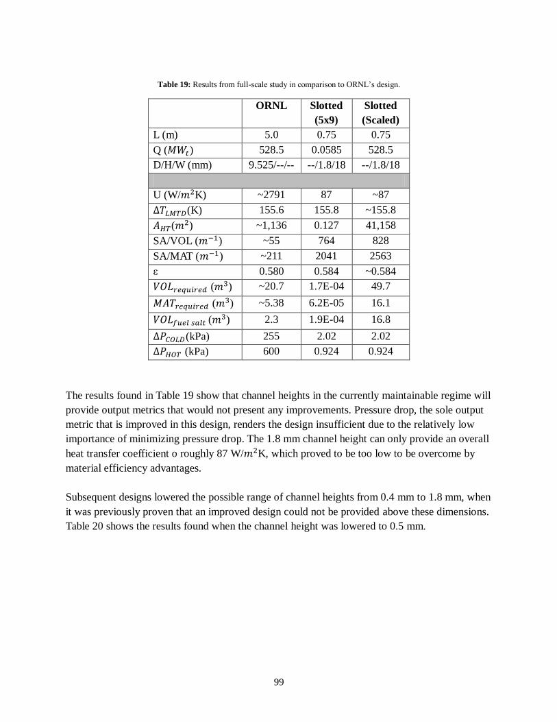
99
Table 19: Results from full-scale study in comparison to ORNL’s design.
ORNL Slotted
(5x9)
Slotted
(Scaled)
L (m) 5.0 0.75 0.75
Q (𝑀𝑊𝑡) 528.5 0.0585 528.5
D/H/W (mm) 9.525/--/-- --/1.8/18 --/1.8/18
U (W/ K) ~2791 87 ~87
𝐿𝑀𝑇 (K) 155.6 155.8 ~155.8
𝐻𝑇( ) ~1,136 0.127 41,158
SA/VOL ( 1) ~55 764 828
SA/MAT ( 1) ~211 2041 2563
ε 0.580 0.584 ~0.584
𝑉𝑂𝐿𝑟 𝑞𝑢𝑖𝑟 𝑑 ( ) ~20.7 1.7E-04 49.7
𝑀 𝑟 𝑞𝑢𝑖𝑟 𝑑 ( ) ~5.38 6.2E-05 16.1
𝑉𝑂𝐿 𝑢 𝑙 𝑠𝑎𝑙𝑡 ( ) 2.3 1.9E-04 16.8
𝑃 𝑂𝐿 (kPa) 255 2.02 2.02
𝑃𝐻𝑂𝑇 (kPa) 600 0.924 0.924
The results found in Table 19 show that channel heights in the currently maintainable regime will
provide output metrics that would not present any improvements. Pressure drop, the sole output
metric that is improved in this design, renders the design insufficient due to the relatively low
importance of minimizing pressure drop. The 1.8 mm channel height can only provide an overall
heat transfer coefficient o roughly 87 W/ K, which proved to be too low to be overcome by
material efficiency advantages.
Subsequent designs lowered the possible range of channel heights from 0.4 mm to 1.8 mm, when
it was previously proven that an improved design could not be provided above these dimensions.
Table 20 shows the results found when the channel height was lowered to 0.5 mm.

100
Table 20: Results from full-scale study in comparison to ORNL’s design.
ORNL Slotted
(5x9)
Slotted
(Scaled)
L (m) 5.0 0.75 0.75
Q (𝑀𝑊𝑡) 528.5 528.5
D/H/W (mm) 9.525/--/-- --/0.5/6 --/0.5/6
U (W/ K) ~2791 289 348
𝐿𝑀𝑇 (K) 155.6 155.5 ~155.5
𝐻𝑇( ) ~1,136 1.01E-04 10,290
SA/VOL ( 1) ~55 1,333 1,562
SA/MAT ( 1) ~211 1,926 2,441
ε 0.580 0.582 ~0.582
𝑉𝑂𝐿𝑟 𝑞𝑢𝑖𝑟 𝑑 ( ) ~20.7 7.6E-08 6.6
𝑀 𝑟 𝑞𝑢𝑖𝑟 𝑑 ( ) ~5.38 5.3E-08 4.2
𝑉𝑂𝐿 𝑢 𝑙 𝑠𝑎𝑙𝑡 ( ) 2.3 1.8E-05 1.2
𝑃 𝑂𝐿 (kPa) 255 287 287
𝑃𝐻𝑂𝑇 (kPa) 600 649 649
The results shown in Table 20 will provide benefits in nearly every metric measured in this study.
Although smaller eddy current probes will be required to be developed for this design, even a
design with channel heights of 1.8 mm will require the development of small-scale pancake
probes that are not currently available. The size of this design will ultimately be determined by
the fouling limit, casting limit of wall thickness, and eddy current probe size. The exact
dimension at which these limitations come into effect is not explicitly known at this point and
will require experimental testing in the future.
Several of the properties taken from ORNL paperwork (Kasten, Bettis, & Robertson, 1966) are
approximated due to the constant evolution of the design of the PHX. Several earlier studies list
values that differ from later Progress Reports, with relatively significant changes taking place
along the way. For example, the 1967 Progress Report mentions that the thermal conductivity of
the molten salts was over-estimated in earlier studies. This was said to have resulted in a 20%
reduction in the overall heat transfer coefficient. Updated values were not concisely written in
the document, so U was assumed to be 80% of the value found in previous documents (Bettis, et
al., 1967).
To approximate a full-scale slotted design, the heat load (Q) was assumed to similar to be that
from ORNL’s design. With the log-mean temperature difference from the 5x9 array paired with

101
an overall heat transfer coefficient scaled to represent its expected value at the necessary number
of channels, the heat transfer surface area, 𝐻𝑇, can be found according to Equation 26.
The overall heat transfer coefficient value in the preliminary 5-channel by 9-channel array
calculations in Table 20 was found by equally weighing the values of the convection heat transfer
coefficient on all channels. Since full-scale arrays of channels (possibly having greater than
1,000 channels in each direction) will be dominated by interior channels and will approach the
value of the average of the interior channels, exterior channels can be ignored due to their
heightened influence from the outer wall boundary condition.
Figure 43 shows the trend of the heat transfer coefficient approaching its total value as the
number of channels approaches 300. With only 45 vertical channels modeled in this study, the
values found in FLUENT would be roughly 97% of the true full-scale value (Kays & London,
1984). The heat transfer coefficients in channels adjacent to the outer wall were found to be
significantly lower than the inner channels, which would be expected to dominate on a full-scale
array. The effect incurred by the phenomena seen in Figure 43 was used in the “scaled”
calculations in Table 20.
Figure 43: Heat transfer coefficient variation based on number of channels modeled (Kays & London, 1984).
The heat transfer performance of ORNL’s shell-and-tube design was better than the relatively un-
optimized slotted design modeled in this study. While it took less than 10% of the material and
roughly 3.5% of the volume to accommodate a similar surface area, more surface area was
needed for the slotted design because of its lower overall heat transfer coefficient. Pressure drops
and effectiveness were maintained to be rather similar for the two designs, with the slotted
design having the ability to improve generously with further optimization and freedom in
temperature boundary conditions. Results from the 5-channel by 9-channel full-length array
showed that, while heat transfer was a detriment, SA/MAT was increased and SA/VOL was

102
dramatically increased in the slotted design. Fuel salt volume was also brought to a much lower
value than that required from the ORNL design.
One detriment to the overall design of the PHX may be the increased pumping power required
for the flow rate and pressure drop incurred in the compact heat exchanger. Although the
pressure drop was equivalent to ORNL’s shell-and-tube design for each fluid, the larger number
of channels sees a greater pumping power, as shown in Equation 46.
Equation 46
where 𝑃 is the pressure drop for each fluid, is the cross-sectional area of each channel, V is
the fluid velocity, and 𝜂 is the pump efficiency (which was assumed to be 90% for this study).
Whereas pumps for the MSBR were designed to be 1400 hp for the secondary coolant and 990
hp for the fuel salt, the slotted heat exchanger design with channel heights of 0.5 mm would
require a pump duty increase by a factor of 10 for the secondary coolant (14,748 hp) and 48 for
the fuel salt (47,832 hp). These are prohibitively high values that would require the use of larger
channels to maintain pump duties on reasonable ranges.
The 1.8 mm channel height, which would also prove to be more robust to fouling and loose
impediments, would also lessen the pump requirement that may make it more reasonable for
commercial use. Pumping power requirements would be lowered by a factor of almost 16 for the
secondary coolant (57.2 hp) and by over 17 for the fuel salt (90.2 hp) for the 1.8 mm channel
height design. Future studied can perform more intense optimization to find the value between
these two data points that provides a reasonable balance of advantages and drawbacks in that
range. The two main data points studied in this thesis can serve as the bounding endpoints for
future optimization studies.
Slotted heat exchangers have the ability to be separated into several banks, varied in dimension
in each direction, or both. Table 21 shows several such possibilities, where N is the number of
banks the slotted heat exchanger is separated into, 𝑁𝑊 is the number of channels in the width-
direction, 𝑁𝐻 is the number of channels in the height-direction, 𝑇𝑂𝑇 𝐿 is the resulting height of
each bank, and 𝑊𝑇𝑂𝑇 𝐿 is the resulting width of each bank.

103
Table 21: Heat exchanger module configuration possible with slotted design.
N
(# banks)
(m)
(m)
L
(m)
VOL
( )
1 1,027 1,027 1.3 6.6 0.75 6.64
4 514 514 0.67 3.3 0.75 6.63
10 325 325 0.42 2.1 0.75 6.62
10 147 721 0.94 0.94 0.75 6.63
16 117 576 0.75 0.75 0.75 6.75
The length of the each module is kept constant at the previously-determined optimal value of
0.75 m. The total volume, VOL, is found to change minimally as the heat exchangers are
separated into up to 16 different banks. Appendix H presents these options in a scaled, graphical
representation that can more succinctly compare the different options available for slotted heat
exchanger banks. A sketch of ORNL’s PHX is also provided for comparison. In-depth studies
should still be completed regarding the optimization of modular heat exchanger banks. Whereas
advantages are seen in separating the exchanger into a large number of banks, corresponding
disadvantages are seen in increased piping requirements and header volume.
IV. Conclusions and Recommendations The results in this study demonstrated the feasibility of an immature, relatively un-optimized
slotted heat exchanger to perform at or above the level of ORNL’s shell-and-tube design in all
metrics used for comparing performance.
In future iterations of this study, an evaluation of wavy channels with constant channel gaps
could be made to enhance heat transfer. If the ability to create a minichannel heat exchanger with
heat transfer performance roughly matching that of the shell-and-tube heat exchangers designed
by ORNL is shown by a minichannel slotted heat exchanger, a slotted heat exchanger could be
shown to be a viable option in commercial nuclear applications. A wavy channel design may
have the ability to allow for eddy current inspection techniques to be used along its length, but
the wavy nature of the channels may induce turbulence to help heat transfer performance.
Another option would be creating very small bars and bumps along the channel surface that will
enhance heat transfer. The pressure drop losses and manufacturing challenges are not expected to
overcome the increased heat transfer performance.

104
Further optimization of channel sizes and shapes can be performed to fully optimize the design.
ProCast can then be utilized to test the validity of casting Hastelloy N on the scale of 1mm in
wall thickness, which is still an unproven concept. Development of high-aspect-ratio eddy
current pancake probes would be another step towards commercial viability.
The ability to contain the PHX within the reactor vessel should be studied in-depth in further
studies. The concept was dismissed here due to the complex nature of piping and altered neutron
performance in this research, but maintaining the PHX within the reactor vessel but outside of
the pool of molten salt, most likely by means of creating a closed portion of the vessel that would
protect the heat exchanger and allow for easier maintenance, is preferred. More complete
knowledge of the exact plant set-up and reactor dimensions must be known before a study can be
launched on this subject.
In the worst possible scenario, a slotted minichannel heat exchanger can present an option for
moving to more compact designs that would bridge the time gap until better maintenance and
inspection techniques can be developed for ultra-compact designs. The performance available
with a slotted heat exchanger is not at the level of other advanced designs, but its ability to more
easily be inspected by well-known methods presents an advantage that has been largely ignored
up to this point in its evolution. The fabrication and manufacturing techniques proposed for this
heat exchanger is expected to offer improvements over advanced techniques necessary for micro-
channel heat exchangers and shell-and-tube heat exchangers.
This study has shown an accurate CFD analysis has been carried out to validate the possibility of
high aspect ratio rectangular channels, being kept within the minichannel regime, to perform at
or above the level of a shell-and-tube heat exchanger in several metrics deemed important for the
MSR PHX application. While engineers at ORNL were constrained to a shell-and-tube design
when the MSBR was planned in the 1960’s, additional considerations were required to assure
that a compact design is feasible in the PHX application.
The work done at ORNL several decades ago was a great starting point for the design of a new
system component, and several of the design considerations made in that study were also carried
out in the PHX study laid out in this research. ANSYS Workbench and FLUENT allowed for
rapid three-dimensional modeling and optimization of several design variables to arrive at the
optimal solution for a slotted heat exchanger.

105
References ANSYS, Inc. (2009). Design Exploration. Canonsburg, PA: ANSYS, Inc.
ANSYS, Inc. (2009). Meshing Help. Canonsburg, PA: ANSYS, Inc.
Ashman, S., & Kandlkar, S. G. (2006). A Review of Manufacturing Processes for Microchannel Heat
Exchanger Fabrication. Fourth International Conference on Nanochannels, Microchannels, and
Minichannels. Limerick, Ireland: ASME.
Beedie, M. (2007, August 10). Thorium: Cleaner Nuclear Power? Retrieved February 8, 2011, from
Power Technology: http://www.power-technology.com/features/feature1141/
Bettis, C. E., Braatz, R. J., Cristy, G. A., Dyslin, D. A., Kelly, O. A., Pickel, T. W., et al. (1967). Design
Study of a Heat-Exchange System for One MSBR Concept. Oak Ridge, TN: Oak Ridge National
Laboratory.
Bettis, C. E., Pickel, T. W., Crowley, W. K., Simon-Tov, M., Nelms, H. A., & Stoddart, W. C. (1971).
Computer Programs for MSBR Heat Exchangers. Oak Ridge, TN: Oak Ridge National Laboratory.
Bhanja, A. (2009). Numerical Solution of Three Dimensional Conjugate Heat Transfer in a Microchannel
Heat Sink and CFD Analysis. Orissa, India: National Institute of Technology, Rourkela.
Burke, O. W. (1972). Hybrid Computer Simulation of the MSBR. Oak Ridge, TN: Oak Ridge National
Laboratory.
Cantor, S., Cooke, J. W., Dworkin, A. S., Robbins, G. D., Thoma, R. E., & Watson, G. M. (1968).
Physical Properties of Molten-Salt Reactor Fuel, Coolant, and Flush Salts. Oak Ridge, TN: Oak Ridge
National Laboratory.
Figley, J. (2009). Numerical Modeling and Performance Analysis of Printed Circuit Heat Exchanger for
Very High-Tempertature Reactors. Columbus, Ohio: Ohio State University.
Gezelius, K. (2004). Design of Compact Intermediate Heat Exchangers for Gas Cooled Fast Reactors.
Cambridge, MA: Massachusetts Institute of Technology.
Greene, S. R., Gehin, J. C., Holcomb, D. E., Carbajo, J. J., Ilas, D., Cisneros, A. T., et al. (2010). Pre-
Conceptual Design of a Fluoride -Salt-Cooled Small Modular Advanced High-Temperature Reactor
(SmAHTR). Oak Ridge, TN: Oak Ridge National Laboratory.
Grimes, W. R. (1967). Chemical Research and Development for Molten-Salt Breeder Reactors. Oak
Ridge, TN: Oak Ridge National Laboratory.
Harvego, E. A. (2006). Evaluation of Next Generation Nuclear Power Plant (NGNP) Intermediate Heat
Exchanger (IHX) Operating Conditions. Idaho Falls, Idaho: Idaho National Laboratory.
Haynes International. (2002). Hastelloy N alloy. Kokomo, Indiana: Haynes International, Inc.

106
Hechanova, A. E. (2007). High Temperature Heat Exchanger Project. Las Vegas, NV: The UNLV
Research Foundation.
I. Allison, N. B. (2009). The Copenhagen Diagnosis, Updating the World on the Latest Climate Science.
Sdyney, Australia: THe University of New Sotuh Wales CLimate Research Centre (CCRC).
International Atomic Energy Agency. (2005). Thorium Fuel Cycle -- Potential Benefits and Challenges.
Vienna, Austria: International Atomic Energy Agency.
Kanaris, A. G., Mouza, K. A., & Paras, S. V. (2004). Designing Novel COmpact Heat Exchangers
forImproved Efficiency Using a CFD Code. 1st Internal Conference "From Scientific Computing to
Computational Engineering". Athens, Greece: IC-SCCE.
Kandlikar, S. G., Garimella, S., Li, D., Colin, S., & King, M. R. (2006). Heat Transfer and Fluid FLow in
Minichannels and Microchannels. Kidlington, Oxford: Elsevier Ltd.
Kasten, P. R., Bettis, E. S., & Robertson, R. C. (1966). Design STudies of 1000-MW(e) Molten-Salt
Breeder Reactors. Oak Ridge, TN: Oak Ridge National Laboratory.
Kays, W. M., & London, A. L. (1984). Compact Heat Exchangers. New York, NY: McGraw-Hill.
LeBlanc, D. (2010). Molten salt reactors: A new beginning for an old idea. Nuclear Engineering and
Design .
Libby, T. M. (n.d.). Testing Critical Medical Tubing Using High Frequency Eddy Current Coils.
Retrieved 2011 24-Feb from Magnetic Analysis Corporation: http://www.mac-
ndt.com/pdf/Hi_Freq_Tube_Testing_Libby.pdf
Lightbridge. (n.d.). Technical Fact Sheet. Retrieved 2011 йил 8-February from Lightbridge:
http://www.ltbridge.com/assets/Thorium_Fuel_Fact_Sheet.pdf
MacPherson, H. G. (1985 15-March). The Molten Salt Reactor Adventure. Nuclear Science and
Enginering , pp. 374-380.
Martin, R. (2011 1-February). China Takes Lead in Race for Clean Nuclear Power. Boulder, CO.
Martin, R. (2009 21-December). Uranium Is So Last Century -- Enter Thorium, the New Green Nuke.
Retrieved 2011 8-February from Wired: http://www.wired.com/magazine/2009/12/ff_new_nukes
McCoy Jr, H. E., & Weir Jr, J. R. (1967). Materials Development for Molten-Salt Breeder Reactors. Oak
Ridge, TN: Oak Ridge National Laboratory.
Mizia, R. E. (2008). Next Generation Nuclear Plant Intermediate Heat Exchanger Acquisition Strategy.
Idaho Falls, Idaho: Idaho National Laboratory.
OECD Nuclear Energy Agency. (2008). Nuclear Energy Outlook. New Milford, CT: OECD Publications.
Olson, L. C. (2009). Materials Corrosion in Molten LiF-NaF-KF Eutectic Salt. Madison, Wisconsin:
University of Wisconsin - Madison.

107
Pra, F., Tochon, P., Mauget, C., Fokkens, J., & Willemsen, S. (2007). Promising designs of compact heat
exchangers for modular HTRs using the Brayton cycle. Nuclear Engineering and Design (pp. 3160-
3173). Amsterdam: Elsevier B.V.
Raghed, M., & Tsoukalas, L. (2010). Global and USA Thorium and Rare Earth Elements Resources. 2nd
Thorium Energy Alliance Conference, The Future Thorium Energy Economy, (pp. 1-17). Mountain View,
California.
Rao, B. P. (2007). Practical Eddy Current Testing. Oxford, UK: Alpha Science International Ltd.
Robertson, R. C. (1971). Conceptual Design Study of a Single-Fluid Molten-Salt Breeder Reactor. Oak
Ridge, TN: Oak Ridge National Laboratory.
Robertson, R. C., Smith, O. L., Briggs, R. B., & Bettis, E. S. (1968). Two-Fluid Molten-Salt Breeder
Reactor Design Study (Status As Of January 1, 1968). Oak Ridge, TN: Oak Ridge National Laboratory.
Rosenthal, M. W., Briggs, R. B., & Kasten, P. R. (1967). Molten-Salt Reactor Program Semiannual
Progress Report for Period Ending February 28, 1967. Oak Ridge, TN: Oak Ridge National Laboratory.
Schobeiri, M. T. (2010). Fluid Mechanics for Engineers. Berlin: Springer.
Shah, R. K., & Sekulic, D. P. (2003). Fundamentals of Heat Exchanger Design. Hoboken, NJ: John
Wiley & Sons.
Shah, R. K., McDonald, C. F., & Howard, C. P. (1980). Compact Heat Exchangers - History,
Technological Advancement and Mechanical Design Problems. New York, NY: American Society of
Mechanical Engineers.
Sohal, M. S., Sabharwall, P., Sharpe, P., & Ebner, M. A. (2010). Engineering Database of Liquid Salt
Thermophysical and Thermochemical Properties. Idaho Falls, Idaho: Idaho National Laboratory.
Solomon, S., Qin, D., & Manning, M. (2007). Climate Change 2007. New York, NY: Cambridge
University Press.
Sunden, B., & Shah, R. K. (2007). Advances in Compact Heat Exchangers. Philadelphia, PA: Edwards.
U.S. Department of Energy and Environmental Protection Agency. (2000). Carbon Dioxide Emissions
from the Generation of Electric Power in the United States. Washington, DC: U.S. Department of
Energy.
U.S. Energy Information Administration. (2010). International Energy Outlook 2010. Washington, DC:
U.S. Energy Information Administration.
Wang, L., Sunden, B., & Manglik, R. M. (2007). Plate Heat Exchangers: Design, Applications and
Performance. Southampton: WIT.
Weinberg, A. M. (1997). The First Nuclear Era, The Life and Times of a Technological Fixer. New York,
NY: Springer.

108
Williams, D. F., Toth, L. M., & Clarno, K. T. (2006). Assessment of Candidate Molten Salt Coolants for
the Advanced High-Temperature Ractor (AHTR). Oak Ridge, TN: Oak Ridge National Laboratory.
World Nuclear Association. (2010 December). World Energy Needs and Nuclear Power. Retrieved 2011
йил 8-February from World Nuclear Association: http://www.world-nuclear.org/info/info16.html

109
Appendix A: ORNL Plant Diagrams
Figure 44: MSBR Plant diagram for Case B (Bettis, et al., 1967)

110
Appendix B: Parametric Mesh Study
Preliminary Mesh Study
Due to the simplistic nature of the geometry used in this study and limited computational
resources available for preliminary studies, a parametric study was performed to test the
minimum coarseness of mesh required to obtain accurate results from FLUENT.
Original mesh distributions were found to be unnecessarily close to the 2 million-node limit, and
results within less than 4% were found with a 995% reduction in node count. The results from
the parametric mesh study will be presented here.
On a 200mm length section of HX, with 𝑁𝑊 and 𝑁𝐻 computed by means of a model
made with 𝑁𝑊 and 𝑁𝐻 . A fine mesh was first developed in order to push the 2
million-node limit imposed on the 2GB RAM processor of the computer in use.
Table 22: Comparison of results for varying mesh counts on small-scale geometry.
Fine Coarse
Length (mm) 200 200
Number of nodes 1,665,464 152,076
Solid element size 1.50E-04 1.20E-03
Fluid element size 3.50E-04 6.00E-04
Sweep Divisions 150 75
Tin % difference N/A 0.164
Tout % difference N/A 1.538
h % difference N/A 3.946
Pin % difference N/A 0.0521
% node reduction N/A 995.1524238
A reduction of almost 1000% of nodes represents a tremendous decrease in computation times.
At a much coarser distribution of nodes, results only 4% different are acceptable for preliminary
studies. For this reason, the element size found for the coarse study will be kept throughout
preliminary computations.
The results of this study are mesh-independent, with the results of this parametric study verifying
the lack of a return for additional nodes above the given concentration.

111
Full-scale Mesh Study
The accuracy of full-scale final results is heavily dependent on the mesh that can be used on a
larger application. With more than twice the number of channels compared to the preliminary
study, the full-scale simulation requires significantly more nodes in its mesh. Channel lengths
were increased to 750 mm in some full-scale simulations, which requires significantly more
nodes than the 200 mm length used in preliminary studies. As mesh element size decreases,
accuracy is gained in results. Fine meshes can be prohibitively resource-intensive with limiting
computing power, so mesh sizes and distributions must be chosen judiciously. This section will
outline the mesh used in full-scale studies (which was taken from the results from the
preliminary study above), a coarser mesh that provided incorrect results, and a very fine mesh
that would be preferred if computational power were increased.
The mesh shown in Figure 45 was used in the final optimized slotted HX design in this study.
Figure 45: Mesh used in full-scale study that reached approximately 1,300,000 nodes.
Figure 46 shows a mesh with significantly less nodes that was used to validate the mesh size and
distribution used in the full-scale study.
Figure 46: Course mesh that contained only approximately 250,000 nodes.

112
Since the results for the full-scale channel array was taken from a previous mesh study
performed on a smaller scale. This process was performed to assure that scaling would not
interfere with the accuracy of results. Table 23 shows the difference between results rendered for
simulations of similar boundary conditions and geometry with the two different mesh
distributions.
Table 23: Full-scale mesh comparison results.
W
(# divisions)
H
(# divisions)
L
(# divisions)
Solid
Divisions
# Nodes % Error
in Po
Fine 30 4 500 2x2 1,191,378 ~5%
Coarse 16 2 250 1x1 165,660 ~35%
Desired
(Very fine)
60 10 1500 4x4 4,000,000+ ~1%
Just as a significant change was found between the two mesh distributions shown in Table 23,
coarser meshes are expected to provide even more accurate results. The 2.5x4.5 array of
channels was deemed sufficiently large to approximate results from a full-scale array of
channels, but available computer imposed a strict restriction in mesh node count. The tradeoff
between capturing more channels to more appropriately simulate a large array of channels
caused mesh element sizes to be raised. Future studies using more powerful computers could use
mesh sizes like those seen in Figure 47.
Figure 47: Desired mesh distribution that contains an estimate of approximately 4,000,000 nodes.

113
Appendix C: Preliminary Study Geometry Calculations
Surface Area Calculation
W H [ ]
W H
Volume Calculation
[ W W ][ H H ][ ]
[ W W ][ H H ][ ]
Material Calculation
[ W H ]
[
W H ]

114
Appendix D: ORNL Shell-and-tube Calculations
The values pertaining to the shell-and-tube PHX designed by ORNL can be found in several
places. Whereas dimensions such as height, values such as the number of tubes, and parameters
such as heat transfer area can be found in HX design documentation (Bettis, et al., 1967), the
volume and material of each type of component inside the heat exchanger (floating heads,
tubesheets, etc) must be estimated from other paperwork.
Sources were found for a single-fluid MSR’s PHX, which had precise material requirements for
a very similar heat exchanger (Robertson R. C., 1971).
Surface Area Calculation
Volume Calculation
ft
Material Calculation
m3 m3 m3 m3
*((
)
) ((
)
)+
*((
)
) ((
)
)+
ft3 m3

115
*((
)
) ((
)
)+
ft3 m3
𝑔
𝑔
ft3 m3
Output Parameter Calculation
(
)
(
)

116
Appendix E: Material Properties
Hastelloy N
Composition (weight %) (Haynes International, 2002)
Table 24: Constituent elements in Hastelloy N.
1 Chromium Molybdenum Iron Silicon Manganese Carbon Co Cu W Al+Ti
71 7 16 5* 1* 0.80* 0.08* 0.20* 0.35* 0.50* 0.35*
1 – Balance * - Maximum
Average Physical Properties
Table 25: Material properties of Hastelloy N (Haynes International, 2002).
Physical Property Temp, °C Metric Units
Density 22 8.86 g/
Melting Range 1300-1400 --
Mean Coefficient of
Thermal Expansion
21-204
21-316
21-427
21-538
21-649
21-760
21-871
21-982
11.6 x m/m-K
12.3 x m/m-K
12.7 x m/m-K
13.4 x m/m-K
14.0 x m/m-K
14.7 x m/m-K
15.3 x m/m-K
15.8 x m/m-K
Thermal Conductivity
100
200
300
400
500
600
700
11.5 W/m-K
13.1 W/m-K
14.4 W/m-K
16.5 W/m-K
18.0 W/m-K
20.3 W/m-K
23.6 W/m-K
Specific Heat
100
200
300
400
480
540
570
590
620
660
680
700
419 J/Kg-K
440 J/Kg-K
456 J/Kg-K
469 J/Kg-K
477 J/Kg-K
485 J/Kg-K
523 J/Kg-K
565 J/Kg-K
586 J/Kg-K
582 J/Kg-K
578 J/Kg-K
578 J/Kg-K

117
Fuel Salt
Table 26: Fuel salt properties (Cantor, Cooke, Dworkin, Robbins, Thoma, & Watson, 1968).
Unit Fuel Salt
Reference Temperature °F 1150
Composition mole % 𝐿𝑖 7 -𝐵𝑒 -
Molecular Weight -- 34
Liquidus Temperature °F 842
Density lb/ 127±6
Viscosity 𝑓 1 1 27±3
Thermal Conductivity Btu 1 1 1 1.5
Heat Capacity Btu 1 1 0.55±0.14
Figure 48: Fuel salts eutectic compositions of LiF, BeF2, and UF4, courtesy of Oak Ridge National Laboratory (Cantor, Cooke, Dworkin, Robbins, Thoma, & Watson, 1968).

118
Coolant Salt
(Sohal, Sabharwall, Sharpe, & Ebner, 2010)
Figure 49: FLiBe properties, courtesy of Idaho National Laboratory (Sohal, Sabharwall, Sharpe, & Ebner, 2010).
Figure 50: FLiBe properties, courtesy of Idaho National Laboratory (Sohal, Sabharwall, Sharpe, & Ebner, 2010).

119
Appendix F: Laminar-Turbulent Transition Discussion
The laminar-turbulent transition remains a relatively unknown science that has garnered
significant research in an effort to find the physics occurring during the process.
For two parallel plates ( =0), the laminar-turbulent has been found to occur at a Reynolds value
of 2500. Square channels ( =1), on the other hand, have been shown to transition at a Reynolds
number of only 200. For any value between these two end data points, linear interpolation can be
used to find the appropriate transition value (Kandlikar, Garimella, Li, Colin, & King, 2006).
Equation 47 shows how the transition Reynolds number can be calculated according to the
channel aspect ratio, .
Equation 47

120
Appendix G: Velocity and Temperature Contours
Temperature profile at half channel width along length of channel
Figure 51: Temperature profile from cold inlet to a channel length of 0.25 m.
Figure 52: Temperature profile from a channel length of 0.25 m to a channel length of 0.5 m.

121
Figure 53: Temperature profile from a channel length of 0.5 m to a channel length of 0.75 m.
Temperature profiles at varying distances along channel length
Figure 54: Temperature profile of geometry cross-section at cold inlet / hot outlet.

122
Figure 55: Temperature profile of geometry cross-section 0.25 m channel length from cold inlet / hot outlet.
Figure 56: Temperature profile of geometry cross-section 0.5 m channel length from cold inlet / hot outlet.

123
Figure 57: Temperature profile of geometry cross-section 0.75 m channel length from cold inlet / hot outlet.
Figure 58: Temperature profile at half channel length, with Symmetry planes mirrored
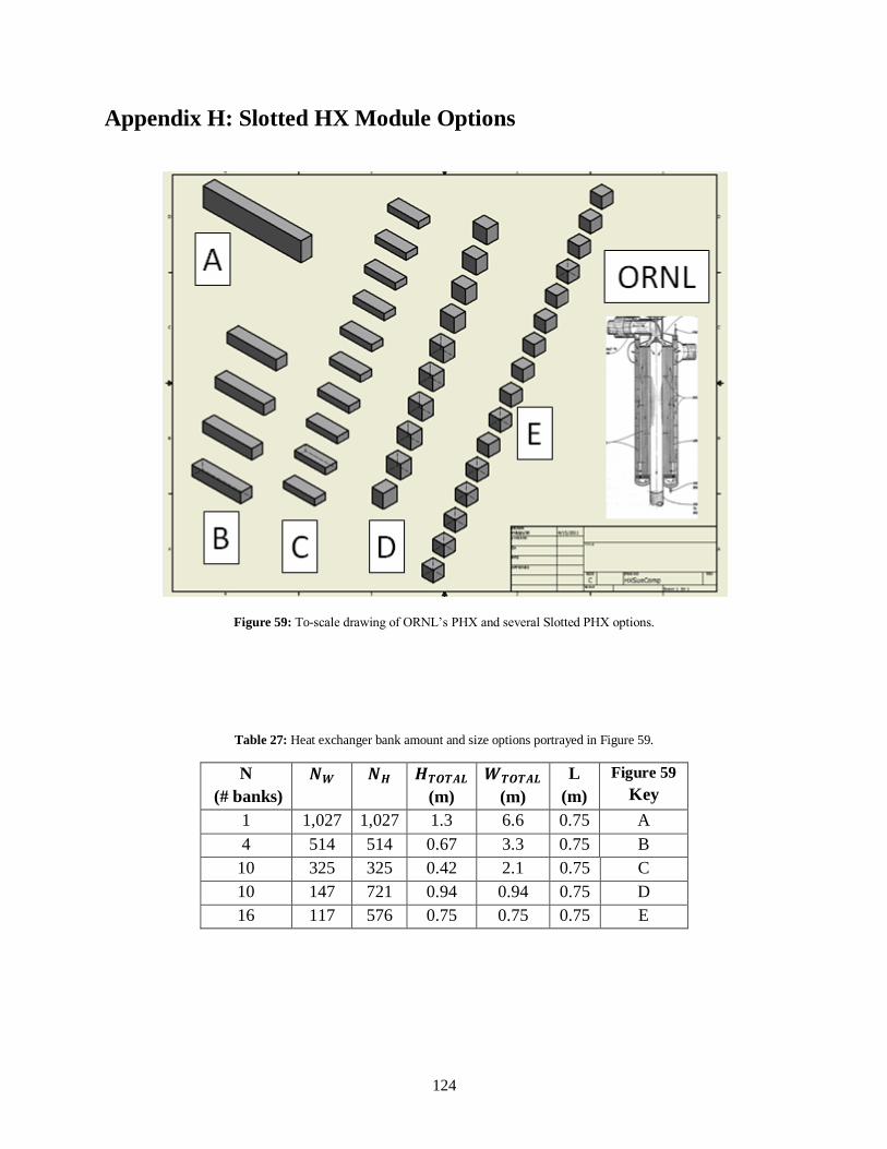
124
Appendix H: Slotted HX Module Options
Figure 59: To-scale drawing of ORNL’s PHX and several Slotted PHX options.
Table 27: Heat exchanger bank amount and size options portrayed in Figure 59.
N
(# banks)
(m)
(m)
L
(m)
Figure 59
Key
1 1,027 1,027 1.3 6.6 0.75 A
4 514 514 0.67 3.3 0.75 B
10 325 325 0.42 2.1 0.75 C
10 147 721 0.94 0.94 0.75 D
16 117 576 0.75 0.75 0.75 E