DEVELOPMENT OF A LOW-DENSITY JET FLOW APPARATUS...
100
DEVELOPMENT OF A LOW-DENSITY JET FLOW APPARATUS by NICHOLAS EDWARD SMITH A THESIS Submitted in partial fulfillment of the requirements for the degree of Master of Science in the Department of Mechanical Engineering in the Graduate School of The University of Alabama TUSCALOOSA, AL 2010
Transcript of DEVELOPMENT OF A LOW-DENSITY JET FLOW APPARATUS...
DEVELOPMENT OF A LOW-DENSITY JET FLOW
APPARATUS
by
NICHOLAS EDWARD SMITH
A THESIS
Submitted in partial fulfillment of the requirements
for the degree of Master of Science
in the Department of Mechanical Engineering
in the Graduate School of
The University of Alabama
TUSCALOOSA, AL
2010

Copyright Nicholas Edward Smith 2010
ALL RIGHTS RESERVED

ii
ABSTRACT
An apparatus was designed and constructed to study supersonic fluid flow in a low
temperature and low pressure environment similar to the same conditions associated with near
space. The apparatus allows the visualization of supersonic flows through an annular nozzle
using a shadowgraph system. The flow system that creates supersonic flows is capable of
producing pulsating jets at virtually any frequency.
This thesis includes details of design of a near space jet flow apparatus that is capable of
producing low temperature and low pressure environment for studying annular jets. The annular
jets are produced from a nozzle that may be later incorporated on near space vehicle. After
testing, it was discovered that the apparatus was capable of producing low temperatures and low
pressures, but the results were inconsistent with a near space environment.
The nozzle being studied has a blocking ratio of 0, 0.5 and 0.75. For each blocking ratio,
the flow is choked, producing a constant mass flow rate. The theoretical and actual thrust were
calculated using propulsion equations. The experimental results were compared to the
theoretical, isentropic results. The jet length was also measured as a reference for vehicle design
limitations. It was found that the maximum experimental thrust coefficients for a nozzle with
blocking ratios of zero, 0.5 and 0.75 were calculated to be 0.430, 0.439, and 0.537 respectively.
All maximum thrust coefficients occur at an ambient pressure of 0.5 kPa.
iii
LIST OF ABBREVIATIONS AND SYMBOLS
Discharge coefficient for theoretical model
Discharge coefficient for nozzle
CV Control volume
e Exiting
i Entering
NSJFA Near space jet flow apparatus
Pressure
Heat transfer
Air gas constant
Temperature
Volume
Work
Mass
Mass flow rate
Specific internal energy
Mach number
Velocity or specific volume
Speed of sound
Specific heat ratio
Force (thrust)

iv
Uncertainty
Time
Change

v
ACKNOWLEDGEMENTS
First and foremost I would like to thank God, my family, and Catherine for supporting
me and providing me the opportunity to continue my education. I would like to thank Dr. John
Baker for allowing me to work in the Aerothermal Sciences Laboratory and continue my
graduate studies in the Department of Mechanical Engineering at the University of Alabama.
Without his guidance, I would not have been able to achieve my dream of receiving a master‟s
degree in mechanical engineering. I would also like to thank my committee members Dr. Bob
Taylor and Dr. Paul Ray.
I would also like to thank Matt Fitzgerald and Arnar Thors from FitzThors Mechanical,
Brandon Griffin, and the employees in the engineering machine shop for assisting me with my
project construction. I would also like to thank Donald Smith from CNX gas for donating
various parts for my project. I also want to thank Jason Cottingham for helping me with my
project construction and Brian Lozes for helping me develop a Matlab code.

CONTENTS
ABSTRACT .................................................................................................................................... ii
LIST OF ABBREVIATIONS AND SYMBOLS .......................................................................... iii
ACKNOWLEDGEMENTS ............................................................................................................v
LIST OF TABLES ......................................................................................................................... vi
LIST OF FIGURES .................................................................................................................... .vii
1. INTRODUCTION .....................................................................................................................1
1.1. NEAR SPACE ....................................................................................................................1
1.2. STATION-KEEPING .........................................................................................................3
1.3. MOTIVATION ...................................................................................................................3
1.4. OUTLINE OF THESIS ......................................................................................................4
2. REVIEW OF LITERATURE ....................................................................................................5
2.1. NEAR SPACE ....................................................................................................................5
2.2. NOZZLES & JET FLOWS ................................................................................................6
3. BACKGROUND .....................................................................................................................10
3.1. JET FLOWS .....................................................................................................................10
3.1.1. CHOKED FLOW...................................................................................................10
3.1.2. MACH NUMBER & FLOW CORRELATIONS..................................................11
3.1.3. NORMAL & OBLIQUE SHOCKS .......................................................................13
3.1.4. THEORETICAL PROPULSION CAPABILITIES ..............................................14
3.1.5. IDEAL NOZZLE FLOW .......................................................................................14
4. THEORETICAL DISCHARGE MODEL ...............................................................................15
4.1. FORMULATION .............................................................................................................15

4.2. IDEAL GAS LAW ...........................................................................................................15
4.3. FIRST LAW OF THERMODYNAMICS: TRANSIENT ................................................16
4.4. THERMODYNAMIC MODEL .......................................................................................16
5. EXPERIMENTAL SETUP ......................................................................................................22
5.1. OVERVIEW .....................................................................................................................22
5.2. THE VACUUM CHAMBER ...........................................................................................22
5.3. THE OBSERVATION CHAMBER.................................................................................23
5.4. VALVE & ACTUATOR ..................................................................................................25
5.5. DATA ACQUISITION SYSTEM ....................................................................................28
5.5.1. MEASUREMENT DEVICES & HARDWARE ...................................................29
5.5.2. DAQ SOFTWARE ................................................................................................33
5.5.3. ADDING A CHANNEL ........................................................................................35
5.6. SHADOWGRAPH SYSTEM ..........................................................................................44
5.7. JET CONFIGURATION ..................................................................................................48
5.7.1. JET HARDWARE .................................................................................................48
5.7.2. JET INSTALLATION ..........................................................................................49
5.7.3. JET FLOW SYSTEM ............................................................................................51
5.7.4. BASIC STAMP FLOW CONTROLLER ..............................................................51
5.8. UNCERTAINTY ANALYSIS .........................................................................................54
5.8.1. MEASUREMENT UNCERTAINTY BACKGROUND ......................................55
5.8.2. LIST OF MEASUREMENT UNCERTAINTY ....................................................55
5.9. THEORETICAL M-FILE ................................................................................................56
6. RESULTS AND DISCUSSION ..............................................................................................58

6.1. THEORETICAL DISCHARGE MODEL ........................................................................58
6.1.1. CASE MATRIX.....................................................................................................58
6.1.2. RESULTS ..............................................................................................................59
6.1.3. DISCUSSION ........................................................................................................61
6.2. EXPERIMENTAL DISCHARGE MODEL.....................................................................61
6.2.1. CASE MATRIX.....................................................................................................62
6.2.2. RESULTS AND DISCUSSION ............................................................................62
7. JET TESTING .........................................................................................................................64
7.1. TESTING METHOD ........................................................................................................64
7.2. RESULTS .........................................................................................................................66
7.2.1. RESULTING EXPERIMENTAL UNCERTAINTY ............................................69
7.3. DISCUSSION ...................................................................................................................71
8. CONCLUSION ........................................................................................................................74
8.1. SUMMARY OF WORK ..................................................................................................74
8.2. FUTURE RESEARCH .....................................................................................................76
9. REFERENCES ........................................................................................................................77
10. APPENDICES .........................................................................................................................80

vi
LIST OF TABLES
Table 1. Coefficients used in calculating equations 21 and 22 ..................................................... 18
Table 2. List of observation chamber components from Duniway Stockroom ............................ 25
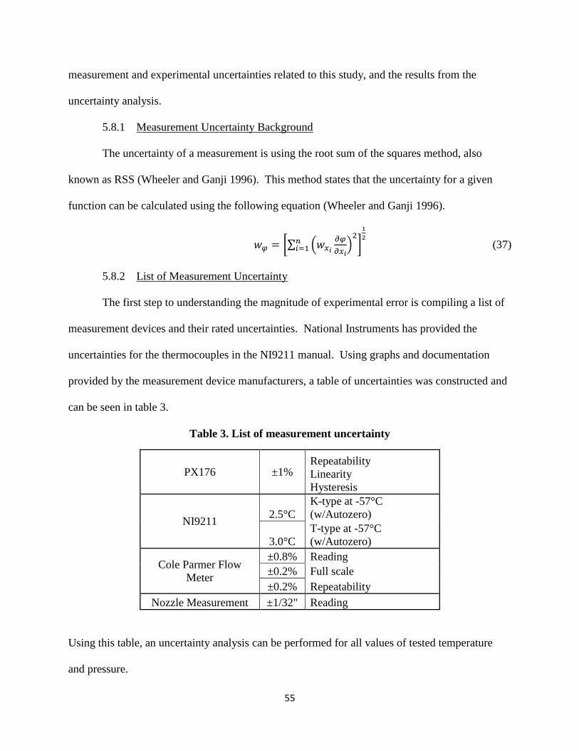
Table 3. List of measurement uncertainty..................................................................................... 55
Table 4. Case matrix for theoretical discharge model .................................................................. 59
Table 5. Sample case for various vacuum chamber pressure settings with observation chamber
kept at atmosphere ........................................................................................................................ 60

vii
LIST OF FIGURES
Figure 1. Earth's Atmosphere .......................................................................................................... 1
Figure 2. Temperatures and pressures associated with Earth's atmosphere (Colozza 2003) ......... 2
Figure 3. Mach number and pressure variations in the C-D nozzle (Nunn 1989) ........................ 12
Figure 4. Diagram of a normal shock (Anderson 2003). .............................................................. 13
Figure 5. System model for NSFJA .............................................................................................. 16
Figure 6. Vacuum chamber dimensions ........................................................................................ 23
Figure 7. Duniway Stockroom CR-1000 CF Cross, Flange OD 10.00”, Tube OD 8.00” used for
main section of observation chamber ........................................................................................... 24
Figure 8. Observation chamber components and configuration ................................................... 24
Figure 9. Apollo 3" full port ball valve with double acting pneumatic actuator .......................... 26
Figure 10. 120VAC solenoid valve (www.omega.com) ............................................................... 27
Figure 11. Diagram of electrical wiring and pneumatic plumbing for actuator and valve ........... 27
Figure 12. NSJFA system setup .................................................................................................... 28
Figure 13. Leak-proof thermocouple used for temperature measurement in observation chamber
....................................................................................................................................................... 29
Figure 14. PX176 pressure transducer and wiring diagram (www.omega.com) .......................... 31
Figure 15. Cole Parmer 5-500 LPM flow meter (www.coleparmer.com) .................................... 32
Figure 16. DAQ Assistant Express VI .......................................................................................... 34
Figure 17. DAQ Assistant properties window .............................................................................. 35
Figure 18. Input measurement option window ............................................................................. 36
Figure 19. „Add Channels to Task‟ window ................................................................................. 37
Figure 20. Maximum, minimum signal input ranges and terminal configuration selection. ....... 38
Figure 21. Creating a new custom scale. ...................................................................................... 39
Figure 22. Custom scale window used to choose scale type ........................................................ 39
viii
Figure 23. Custom scale window .................................................................................................. 40
Figure 24. Pressure versus temperature plot used to obtain slope and y-intercept for PX176 25
psia pressure transducer scale ....................................................................................................... 41
Figure 25. DAQ Assistant equipped with a signal splitter located in the block diagram window of
LabVIEW ...................................................................................................................................... 42
Figure 26. LabVIEW controls window used to select method of viewing signals ....................... 42
Figure 27. LabVIEW's Write to Measurement File assistant ...................................................... 43
Figure 28. Schematic of measurement system components ......................................................... 44
Figure 29. Basic setup of shadowgraph system used for viewing annular jets............................. 45
Figure 30. Electrical circuit for light source used in shadowgraph system .................................. 46
Figure 31. Concave mirror used in shadowgraph system ............................................................. 47
Figure 32. Proper adjustment schematic for shadowgraph system ............................................... 48
Figure 33. Components of jet nozzle ............................................................................................ 49
Figure 34. Jet configuration inside observation chamber ............................................................ 50
Figure 35. Projection of nozzle edge and test area from shadowgraph system ............................ 51
Figure 36. BASIC Stamp code used to initiate solenoid valve pulsation in jet flow system (Pike
2010). ............................................................................................................................................ 52
Figure 37. Overhead view of jet flow system with circuit ............................................................ 54
Figure 38. Sample pressure and temperature response from experimental pseudo-algorithm m-
file ................................................................................................................................................. 56
Figure 39. Theoretical results of NSJFA plotted against atmosphere P-T curve .......................... 60
Figure 40. Plot of experimental data from approximately fifty test runs ..................................... 62
Figure 41. Sample snapshot of pulsating jet with zero blocking ratio and NSJFA pressure at 15
kPa................................................................................................................................................. 65
Figure 42. Compilation of annular jet structures for NSJFA pressures between 0.5 kPa and 100
kPa................................................................................................................................................. 66
Figure 43. Visual jet length for nozzle with three blocking ratios ................................................ 67

ix
Figure 44. Theoretical (isentropic) thrust capabilities .................................................................. 68
Figure 45. Calculated experimental thrust for three nozzle blocking ratios ................................. 68
Figure 46. Calculated experimental thrust coefficient .................................................................. 69
Figure 47. Experimental uncertainties of thrust calculation for nozzle with blocking ratio of a)
zero, b) 0.5, and c) 0.75 ................................................................................................................ 70
Figure 48. Structure of an overexpanded jet (Scott 2005). .......................................................... 72
Figure 49. Block diagram in LabVIEW data acquisition ............................................................. 84
Figure 50. Front panel window used in LabVIEW data acquisition ............................................. 85
Figure 51. Nozzle end cap dimensions ......................................................................................... 86
Figure 52. Nozzle flow straightener dimensions .......................................................................... 86
Figure 53. Blocking bar dimensions ............................................................................................. 87
Figure 54. Nozzle cone section dimensions .................................................................................. 87

1
1. INTRODUCTION
1.1 Near Space
Near space is defined as the region of the atmosphere ranging from altitudes of 18.9
kilometers to 30 kilometers (Colozza 2003). This range covers the upper portion of the
troposphere, the Tropopause, and the lower third portion of the stratosphere. Figure 1 displays
the profile of Earth‟s atmosphere (Colozza 2003).
Figure 1. Earth's Atmosphere
There has been a significant increase of interest in near space within the past two decades
since the development and use of vehicles in near space can provide platforms for a variety of
scientific, commercial, and military applications in a cost effective manner (Cao and Baker
2008). The startup costs of systems that operate in near space are inexpensive when compared to
the startup cost of systems that operate in outer space (Tomme 2005). The time to develop near
space systems is also less extensive. Many of the same results from projects involving systems

2
in outer space that required millions of dollars and many years to develop can be obtained from
near space for a fraction of the cost and time. Because near-space systems are closer to the
earth, visual results involving pictures or video can be obtained at a higher resolution and better
sensitivity (Colozza 2003).
Near space has extremely low temperatures, low pressures, and may have high wind
velocities. These conditions must always be considered when designing systems to operate in
near space. Figure 2 shows the temperatures and pressures associated with near space. The plot
was generated based on data from U.S. Standard Atmosphere (Munson, Young and Okiishi
2006). This figure will be referenced throughout this document as a basis for design and
calculation. The a chart of altitudes with theses associated temperatures and pressures can be
seen in Appendix A.
Figure 2. Temperatures and pressures associated with Earth's atmosphere (Colozza 2003)
0
20
40
60
80
100
120
0
50
100
150
200
250
300
350
0 5000 10000 15000 20000 25000 30000
Pre
ssu
re (
kP
a)
Tem
per
atu
re (
K)
Altitude (m)
Temperature Pressure

3
1.2 Station Keeping
The potential to develop vehicles for extended flight in near space has motivated
engineers and scientists. This study will focus primarily on the propulsion capabilities of
supersonic annular jets for station keeping capabilities for a near space vehicle. The jets studied
in this experiment may be utilized as a resource to hold a static position for a high altitude
vehicle if coupled with a control system and other necessary components.
1.3 Motivation
The purpose of this study was to build an apparatus that could simulate pressures and
temperatures associated with near space and to examine the impact of decreasing pressure and
temperature on the thrust capabilities of annular jets. Supersonic flows will likely exist in
propulsion systems used to achieve station-keeping capabilities for near space vehicles. In order
to study how these jets perform in near space, the jets must be studied in a similar environment.
Upon completing a literature survey, many research opportunities were presented. By
constructing a near space jet flow apparatus, future research may include the study of multiple
types of jets, subsonic or supersonic, with capabilities of pulsation at virtually any frequency.
The near space jet flow apparatus may also allow the study of maximizing nozzle efficiency by
modification of nozzle geometries. To quantify jet capabilities, it is desired to have the
apparatus measure jet flow rates and view the jets using a shadowgraph system.
The first objective of this study was to design a near space jet flow apparatus (NSJFA) to
simulate the temperatures and pressures in near space. The apparatus was designed to be
optically accessible in order to visualize the structure and behavior of the annular jets. During
the design process, three designs were considered, but only one NSJFA design was found to be
practical.

4
The second objective of this study was to specify, locate, and purchase the necessary
components and build the NSJFA. Materials and measurement devices were selected based on
their ability to withstand low temperatures and pressures. Some of the NSJFA components were
machined to meet the design specifications. Custom nozzles were also machined to create the
annular jets.
The third objective of this study was to visualize the flow of the annular jets and use the
measurement devices to quantify the thrust capabilities. It was desired to test the nozzle with
three blocking ratios under multiple chamber pressures and temperatures corresponding to 1976
Standard Atmosphere values. It is desired to obtain various flow characteristics as a function of
pressure, temperature, and blocking ratio.
1.4 Layout of Thesis
This thesis will discuss the study of annular jets in high altitude conditions. The results
from a literature survey of near space, jet flows, and flow visualization will be discussed in the
next chapter. The third chapter will discuss the theoretical model of the NSJFA system and the
engineering principles linked to the formulation of the model and the development of the pseudo-
algorithm used to calculate the change in temperature and pressure. The fourth chapter of this
thesis will discuss the physical model of the NSJFA. This includes an in-depth explanation of
the chambers, measurement devices, the flow visualization system, data acquisition system, and
jets used in this experiment. The sixth chapter will discuss the theoretical and experimental
results of the NSJFA and the seventh chapter will discuss the theoretical and experimental results
of the jet flows including an uncertainty analysis of thrust calculation. The eighth and final
chapter will conclude this thesis by summarizing results and making suggestions and
recommendations for future research and experiments.
2. REVIEW OF LITERATURE
2.1 Near Space
Near space is the region above earth‟s atmosphere ranging from 18.9 kilometers to 30
kilometers (Colozza 2003). The lower boundary of 18.9 kilometers has been established in order
to be greater than the current International Civil Aviation Organization (ICAO) airspace limit of
approximately 18.2 kilometers (Tomme 2005). Research has shown that the conditions in near
space are quite harsh in comparison to conditions on Earth. The temperature in near space can
reach as low as -60ºC while the absolute pressure can reach as low as 0.01 times that experienced
at sea level (Cao and Baker 2008). The wind velocities in near space depend on the geographical
location and altitude and can reach can reach speeds up to 70 meters per second (Colozza 2003).
These low temperatures, low pressures, and high wind velocities present a multitude of
challenges in the development of near space vehicles.
Flying for an extended period of time in near space has been long sought by researchers,
engineers, and scientists. Because of these low temperatures and low pressures, extended time of
flight in near space is difficult because of the lack of air to produce lift forces on an aircraft
(Young, Keith and Pancotti 2009). Plane-like aircrafts cannot typically fly in near space unless
traveling at a high speed or equipped with large wingspans (Young, Keith and Pancotti 2009).
These types of aircraft may be equipped with a propulsion system and require a sustainable
power system with a high energy density for extended-time flight (Williams, Marcel and Baker
2007).

6
It is desired to have a near space vehicle maintain itself for an extended period of time
regardless of the altitude and weather conditions (Williams, Marcel and Baker 2007). Another
type of near space aircraft that has been researched are high-altitude balloons. As of 2003,
multiple concepts and designs were being developed by companies and government agencies
around the world including Lockheed Martin, Techsphere Systems International, Japan‟s
National Aerospace Laboratory, the European Space Agency, and Skycat Technologies (Colozza
2003). High-altitude balloons can be utilized in near space, but current balloon designs have no
means of steering or propulsion (Young, Keith and Pancotti 2009). Should a high altitude
balloon be equipped with a propulsion system, thrust to overcome drag due to high-altitude
winds must be considered in the design for the balloon to move or stay in a fixed position.
According to one study, “advanced concepts for near-space propulsion systems must be able to
produce force levels of 100N to 100kN to be of use on near-term near-space dirigibles” since
“proposed near-space dirigibles commonly have diameters of greater than 20 meters” (Young,
Keith and Pancotti 2009). The development of these propulsion systems for use in near space
presents part of the motivation for this study as well the production of a near space environment
for the study of these potential propulsion systems.
2.2 Nozzles & Jet Flows
There are a broad range of research topics involving supersonic jets. One of the focuses
of this study is to create a device to research the structure of jets in near space conditions and
also using compressible fluid as means of propulsion. Since these two topics are of importance,
literature involving research of supersonic flows, nozzles, and imagery are considered.
One topic of research involving supersonic flow is the design of supersonic nozzles. In
an extensive study conducted in 1959, criteria are addressed for designing an annular nozzle for a
7
given gas with a constant specific heat ratio such that no shockwaves or limit lines exist inside
the nozzle (Lord 1961). Lord‟s study explains in great detail what happens in nozzle flow in a
converging-diverging (CD) nozzle. Although this study will not involve a CD nozzle, knowing
what physical phenomena can occur in compressible nozzle flow can be quite helpful.
Understanding how to design a nozzle for maximum efficiency is presented and should be
referenced for future research. Another study has explained the separation of supersonic flows
inside CD nozzles. The fluid separations in CD nozzles occur due to operation at low pressure
ratios below the design value of the nozzle and results in shocks produced inside the nozzle
(Papamoschou, Zill and Johnson 2008).
In order to contest nozzle inefficiencies, recent experiments have been performed to
make nozzles more efficient. In rocket nozzles, as altitude increases, propulsion from nozzles
becomes less efficient due to a difference in exhaust gas pressures and ambient pressures.
(Stoffel 2009). The same is true for non-rocket nozzles. In a recent experiment performed in
2009, an annular insertion known as an “aerospike” was used to study propulsion capabilities in
a conical nozzle. The purpose of this study was to minimize “over expansion,” a condition that
causes exhaust gases to separate from nozzle walls and diminish thrust capabilities (Stoffel
2009). According to this study, when the exhaust gas pressure is equal to ambient pressure, a
conical nozzle is performing at maximum efficiency (Stoffel 2009). Jet flows corresponding to
this pressure ratio of unity produce a column shaped exhaust plume, indicative of isentropic flow
(Stoffel 2009) (Anderson 2003). Jet flows corresponding to a back pressure to exit pressure ratio
greater than unity produce an expanding jet, which reduces nozzle efficiency (Stoffel 2009).
Results from these experiments showed that using an annular aerospike can produce up to 95%
nozzle efficiency (Stoffel 2009). Although an aerospike protrudes from the nozzle exit, allowing

8
the exiting flow to attach itself to the aerospike walls at low ambient pressures, the main
objective learned from this study is that a nozzle equipped with an annular blockage may be
more efficient than a nozzle without. Since the demand for producing more efficient propulsion
systems exist, the study of supersonic annular jets will be presented in this thesis.
In combination with making nozzles more efficient by using rigid geometrical structures,
previous research of jet flows also includes pulsation. One particular study has used the
propulsion schemes of squid as motivation to study jet pulsations. The source indicates that
squid are the fastest of all swimming invertebrates due to their “ideally streamlined
configuration” and unique means of propulsion using pulsation (Mohensi 2006). Other research
has shown that an incompressible pulsating jet, having no flow between pulsations, could
produce 90% higher thrust than an un-pulsed jet (Krueger and Gharib 2005). While this
particular study in 2005 examined the effects of pulsation using an incompressible fluid, it is
desired to obtain more knowledge about the effects of pulsation in supersonic flow. Another
source states that an interesting phenomenon of pulsating jets is penetration depth. Pulsating jets
have the capability to penetrate cross flow up to five times greater than steady jets, making them
more effective for propulsion in near space‟s high winds (Olden, et al. 2005). A particular
motivation of this project is to create a pulsating jet system with supersonic flow for future
research.
It is also important to visualize high speed flows and study the structures under different
conditions in order to determine appropriate application. Upon completing a literature survey,
the most common tool for flow visualization is the Schlieren system. According to a recent
study, several other methods of studying supersonic jets are being utilized, such as rainbow
Schlieren deflectometry, which measures density profiles, and Mach Zehnder interferometry,
9
which can measure the field density of a circular supersonic jet (Kohle and Agrawal 2009).
Other techniques include laser beam deflection, which measures density points in a supersonic
nitrogen jet, and planar nitric oxide laser induced fluorescence that can be used to measure scalar
properties such as pressure and temperature in an underexpanded jet (Kohle and Agrawal 2009).
One easy method of visualizing high speed fluid flows is using a shadowgraph system, where the
linear displacement of disturbed light is measured (Goldstein 1996). A shadowgraph system is
generally low-cost and can easily be set up. (Olden, et al. 2005). The resulting projections from
a shadowgraph produce a two dimensional image of a three dimensional shock structure (Olden,
et al. 2005). It was decided that based on cost and available parts, a shadowgraph system would
be the visualization system used for this study.

10
3. BACKGROUND
3.1 Jet Flows
Fluid flow is an entity often studied in science and engineering. There are multiple types
of flows defined by multiple types of properties and characteristics. For this study, compressible
flow is considered. This is due to the fact that the annular jet studied in this experiment will
produce high velocity flow rates which can cause substantial changes in fluid density and
justifies the assumption that the variation of density and other fluid property relationships will
require attention (Munson, Young and Okiishi 2006). Depending on the jet flow velocity, the
compressible flow may be considered subsonic, transonic, supersonic, or hypersonic (Anderson
2003). For each monitored flow, it is desired to predict the phenomenon that occurs at the nozzle
exit using compressible flow relationships. The following section will discuss and explain the
variation of jet flows, the difference between each, and how the scientific discussion of these
flows will be applied to this study.
3.1.1 Choked Flow
Pressure differences are the driving force of fluid flow. “Choked flow” is a common
occurrence in compressible flows especially flows that have high stagnation pressures. When a
nozzle is choked, the mass flow rate stays constant. With fixed stagnation and ambient
pressures, the only way that mass flow rate can be increased is to increase the throat area in
which the compressible fluid is flowing or decreasing the stagnation temperature of the fluid
(Nunn 1989). In typical applications involving air, flow becomes choked through an orifice

11
when the back pressure to stagnation pressure ratio is less than or equal to 0.528, assuming the
flow is isentropic, one-dimensional, and has constant specific heats.
3.1.2 Mach Number & Flow Correlations
The fluid used in this study of annular jets is air, an ideal gas. The Mach number for an
ideal gas can be calculated using the equation below.
(1)
It is better understood as the ratio of the local speed of flow and the speed of sound in the
flowing fluid. It is a measure of the extent to which the flow is compressible or not (Munson,
Young and Okiishi 2006).
For compressible flows, changes in entropy are of particular importance. Isentropic flow
is flow with constant entropy. This flow is particularly desirable in air jets because it is
considered efficient since it is theoretically adiabatic, frictionless, and reversible. It is desired to
have this study reveal an optimal setting for the annular jets by pinpointing if and when
isentropic flow is found.
It is necessary become familiar with compressible subsonic flows since the annular jets
being studied possibly involve flow for which 0.3 < Ma < 1.0. Transonic flow is when the Mach
number remains subsonic, sufficiently near unity, but other regions of the flow may produce a
pocket of logically supersonic flow. Supersonic flow is a flow field where the Mach number is
greater than unity (Anderson 2003).
In a converging-diverging nozzle, also known as a C-D nozzle, several different
phenomena may occur depending on the pressures associated with the flow. Although the
nozzles used in this experiment are not C-D nozzles, resulting exit phenomena may still be the
same. These relationships can be seen below in figure 3.

12
Figure 3. Mach number and pressure variations in the C-D nozzle (Nunn 1989)
It must be noted that at some pressure, isentropic flow throughout the nozzle theoretically occurs.
This shows that isentropic flow results in no shock production. It must also be noted that the
Mach number for isentropic flow through a nozzle throat is unity.
The pressure and temperature at the throat of a C-D nozzle can be calculated using the
relationships:
(2)
(3)

13
The theoretical maximum flow rate for a choked nozzle during isentropic flow can be found
using the equation
(4)
3.1.3 Normal & Oblique Shocks
A normal shock wave is a phenomenon that occurs in supersonic, one-dimensional flow.
One-dimensional flow is considered flow in which the properties only vary in one direction as
seen below in figure 4.
Figure 4. Diagram of a normal shock (Anderson 2003).
It can be seen that the flow behind a shock wave is supersonic and the flow downstream
of a shock wave is subsonic. The shock itself is a very thin region, typically 10-5
cm for air at
standard conditions (Anderson 2003). Normal and oblique shock waves are created by
disturbances which propagate by molecular collisions at the speed of sound. Oblique shocks

14
form at angles less than ninety degrees when supersonic flow is “turned into itself” (Anderson
2003).
3.1.4 Theoretical Propulsion Capabilities
Thrust from an isentropic jet can be calculated using the equation below (Sutton and
Biblarz 2010).
(5)
It can be seen that the maximum thrust for any given nozzle is found in a vacuum where the
ambient pressure Pa equals zero (Sutton and Biblarz 2010). The flow is supersonic so the nozzle
exit pressure Pe may be different than the ambient pressure. The thrust coefficient represents the
amplification of thrust due to the expansion of gas in a supersonic nozzle in comparison to the
thrust that would occur if the chamber pressure acted over the throat area only (Sutton and
Biblarz 2010). If the actual mass flow rate is known, the discharge coefficient can be equated
using the ratio below.
(6)
3.1.5 Ideal Nozzle Flow
Many assumptions are considered for an ideal nozzle flow. The working fluid must be
gaseous and obey the perfect gas law. Heat transfer across the rocket walls must be zero, which
insists that the flow through the rocket is adiabatic. An ideal rocket must also have no shock
waves or discontinuities in the nozzle flow, which insists that the gas velocity, pressure,
temperature and density are all uniform across the nozzle exit. All of these assumptions are
consistent with an isentropic solution and are considered when performing the calculations of
equations 4 and 5 (Sutton and Biblarz 2010)
4. THEORETICAL DISCHARGE MODEL
4.1 Formulation
From the ideal gas law, a rapid compression or expansion of gas within a control volume
will produce a noticeable change in temperature. Understanding that the expansion of an ideal
gas within a control volume yields low temperatures and pressures is the key component to
creating an NSJFA. The following chapter will discuss the theory behind a “discharge model”
using engineering principles and mathematics.
4.2 Ideal Gas Law
In thermodynamics, the ideal gas law states that a change in gas density is directly related
to changes in pressure and temperature. The relationship can be seen below.
(7)
Internal energy, a microscopic form of energy related to the molecular structure of a
system and the degree of the molecular activity, is the sum of all microscopic energy and is
typically denoted by “u” (Cengal and Boles 2008). Enthalpy is known as a combination
property and is given by:
(8)
Two other useful rules are the enthalpy and entropy of an ideal gas are strictly functions
of temperature:
(9)
(10)
4.3 First Law of Thermodynamics: Transient
The first law of thermodynamics states that energy can be cannot be created or destroyed,
but only transformed from one state to another (Cengal and Boles 2008). It is given by the
equation shown below.
(11)
As mentioned in section 3.1, thermodynamic principles govern the dynamics of the NSJFA
system. Rapid evacuation of an ideal gas within a control volume will create a drop in
temperature and pressure and it is desired to numerically predict these values in order to validate
the possibility of creating a near space environment. Although it is not necessary to dwell on the
transient response of the system, it must be modeled in order to predict what is happening during
rapid evacuation of the NSJFA. Using thermodynamic principles and mathematics, a steady-
state response follows the transient response. This allows a validation of the discharge model as
well as limitations and design specifications for measurement devices and components.
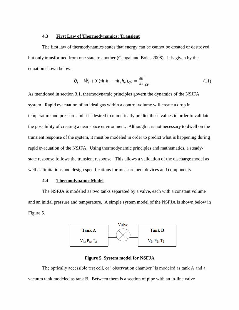
4.4 Thermodynamic Model
The NSFJA is modeled as two tanks separated by a valve, each with a constant volume
and an initial pressure and temperature. A simple system model of the NSFJA is shown below in
Figure 5.
Figure 5. System model for NSFJA
The optically accessible test cell, or “observation chamber” is modeled as tank A and a
vacuum tank modeled as tank B. Between them is a section of pipe with an in-line valve

17
attached. Once the valve is opened instantaneously, an immediate exchange of energy occurs
from state 1 at t = 0 to state 2 at t = t + . The rapid discharge theoretically causes an
immediate drop in temperature and pressure in tank A while the temperature and pressure in tank
B rise.
The first step in determining the changes in the tanks is calculating the initial mass using
the following ideal gas law equations:
(12)
and likewise,
(13)
The mass of air in the tanks at the t = t + can be solved for by developing similar equations
and the total mass of air in the system can be shown as
(14)
The initial densities in tank A and tank B can be calculated by using
(15)
and likewise,
(16)
A control volume is drawn surrounding the outer boundary of the tanks. It is also assumed that
the system transfers no heat to the surroundings and does no work. By making these
assumptions, the first law of thermodynamics for modeling a rate change of energy in tank A can
be rewritten as
(17)

18
and additionally to model the rate change of energy in tank B,
(18)
Since flow will be only in one direction, the sum of the energy entering tank A and the sum of
the energy leaving tank B are zero. The equation can be rewritten as
(19)
and likewise for tank B,
(20)
From the conservation of mass, the rate change of mass leaving tank A is equal to the opposite
rate change of mass entering tank B and for a throttle, the enthalpy exiting tank A is equal to the
enthalpy entering tank B. The specific enthalpy or enthalpy per unit mass, in either tank can be
found using the polynomial expression
(21)
The specific internal energy, or energy per unit mass, is also a function of temperature alone due
to air being an ideal gas. The specific internal energy for either tank can be found using the
polynomial expression
(22)
The coefficients α, β, γ, and δ used to calculate the specific enthalpies and internal energies can
be seen below (Cengal and Boles 2008).
Table 1. Coefficients used in calculating equations 21 and 22
h u
α 1.14610 × 10⁻⁷
1.18900 × 10⁻⁷
β -7.36918 × 10⁻⁵
8.00883 × 10⁻⁵
γ 1.01720 0.732878
δ -1.44501 1.78317

19
Using results from equations 12, 13, and 22, the internal energy can be calculated by using
(23)
and similarly,
(24)
The mass flow rate of air from tank A to tank B can also be calculated. The mass flow rate
equation for non-choked flow (PA/PB>0.528) can be seen below (Kruger 1999).
(25)
The equation for choked flow (PA/PB < 0.528), also known as Ramskill‟s equation, can be seen
below (Kruger 1999).
(26)
For each case, frictional losses are neglected and the discharge coefficient C is assumed to be
unity. Since mass flow rate can now be calculated, the change in mass between the tanks during
instantaneous valve opening can be determined using the equations 12, 13, and 27 or 28 with
numerical integration, known as Euler‟s method, to form the following equations (Tipler and
Mosca 2008).
(27)
(28)
Notice that this equation is not exact, but approximate because the mass flow rate experienced
after the first time step is used to calculate the new mass in tank A and tank B. However, when
time step Δt is extremely small, the results are quite accurate. Using the calculated results from
equations 23, 24, 33, 34, and 25 or 26, a new internal energy can be solved for using

20
(28)
(30)
With this new internal energy value, equations 31 and 32 are utilized to find a new specific
internal energy in tank A and tank B and are given by
(31)
(32)
Using this new specific internal energy value, the inverse of equation 22 is used to calculate a
new temperature for the air in tank A and tank B and are shown below. These new temperature
equations were found by plotting equation 22 in Microsoft Excel with internal energy on the x-
axis and temperature on the y-axis. A fourth order polynomial fit trendline was then plotted and
the “Display Equation on Chart” option was chosen, giving a temperature equation as a function
of specific internal energy.
(33)
(34)
The α, β, γ and δ used in these equations are -3.81886 × 10⁻⁷
, 1.68752 × 10⁻⁴
, 1.374875, and
1.68773 respectively. The new pressure in tank A and tank B can be calculated using this new
temperature and mass value. The equations for the new pressure calculations are shown below.
(35)
(36)

21
With these new pressure calculations, a new density can be solved for using equations 18 and 19,
and starting at equation 16, the calculation process can be repeated for temperatures and pressure
in tank A and tank B after another time step Δt.

22
5. EXPERIMENTAL SETUP
5.1 Overview
As previously stated, the purpose of this study was to examine pulsating jets in a near
space environment. As mentioned in section 3.4, the system can be modeled as two tanks
separated by a valve. Temperature and pressure of both tanks must be measured. The NSJFA
must be optically accessible to view the jet structure of the pulsating jets. The flow of the
pulsating jets must also be measured. The following chapter will discuss the physical
components of the NSJFA, the measurement devices used with an analysis of uncertainty, the
design of the jet nozzles, and a justification of these devices using the thermodynamic model.
5.2 The Vacuum Chamber
As mentioned in chapter 1, a near space environment yields temperatures as low as 216 K
and absolute pressures as low as 1.2 kPa . In order to create these low temperatures and
pressures, a vacuum chamber must be used. Using the thermodynamic model, one can see that a
large volume tank in comparison to the other tank is critical for producing extremely low
temperatures and pressures. Figure 6 shows the physical dimensions of the vacuum chamber
used in this experiment.
23
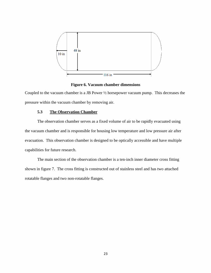
Figure 6. Vacuum chamber dimensions
Coupled to the vacuum chamber is a JB Power ½ horsepower vacuum pump. This decreases the
pressure within the vacuum chamber by removing air.
5.3 The Observation Chamber
The observation chamber serves as a fixed volume of air to be rapidly evacuated using
the vacuum chamber and is responsible for housing low temperature and low pressure air after
evacuation. This observation chamber is designed to be optically accessible and have multiple
capabilities for future research.
The main section of the observation chamber is a ten-inch inner diameter cross fitting
shown in figure 7. The cross fitting is constructed out of stainless steel and has two attached
rotatable flanges and two non-rotatable flanges.

24
Figure 7. Duniway Stockroom CR-1000 CF Cross, Flange OD 10.00”, Tube OD 8.00” used
for main section of observation chamber
After selecting the main section of the observation chamber, other components were chosen
based on design parameters, functionality, and availability. The configuration of the components
used to construct the observation chamber can be seen in figure 8 and table 1 lists these
components in detail.
Figure 8. Observation chamber components and configuration

25
Table 2. List of observation chamber components from Duniway Stockroom
Component Description Duniway Part Number
1 6” OD 4”viewport VP-600-400
2 10” – 6” reducer flange A1000X600T
3 10” blank flange F1000-000N
4 8” tube OD nipple fitting NP-800
5 10” – 8” reducer flange A1000X800T
6 8” – 6” reducer flange A800X600T
7 6” tube )D tee TE-800
8 6” blank flange F600-000N
The observation chamber is made optically accessible using viewports on opposite sides of the
ten inch cross fitting. The flanges and fittings are bolted together using 5/16 inch, 24 threads-
per-inch, twelve point bolts and flange nuts. Between each fitting and flange connection is an
appropriately sized Viton® gasket. Duniway Stockroom uses a vacuum furnace system to
ensure that all purchased Viton® gaskets are degassed to minimize leaks.
5.4 Valve & Actuator
As mentioned in section 3.1, it is desired to rapidly discharge the observation chamber to
create extremely low temperatures. This is because the observation chamber cannot be perfectly
insulated and impinging heat transfer can enter the system causing the temperature to increase
inside of the observation chamber. Apollo valves technical and sales support was consulted for
proper three inch valve specification. An Apollo, three inch, 87A-200 Series stainless steel,

26
ANSI class 150 flange, full port ball valve, shown in figure 9, was used to achieve rapid
decompression of the observation chamber.
Figure 9. Apollo 3" full port ball valve with double acting pneumatic actuator
This valve is capable of withstanding low temperatures and is designed to see high cyclic duty.
Apollo boasts that no maintenance is required up to 20,000 cycles.
The three inch full port ball valve is equipped with a pneumatic actuator capable of
opening the valve in 0.72 seconds. The double-acting pneumatic actuator is activated using a
three way switch connected to four, 120VAC solenoids shown in figure 10. These solenoid
valves are supplied with 110 psig air from a DeWalt electric air compressor.

27
Figure 10. 120VAC solenoid valve (www.omega.com)
Two of the 120V solenoids are wired to open when the three way switch is in a far
position causing the valve to open. The other two 120VAC solenoids are wired to open when the
switch is placed in the opposite position, causing the valve to close.
Figure 11. Diagram of electrical wiring and pneumatic plumbing for actuator and valve

28
The actuator, given an air supply of 110 psi, produces an astounding 400 ft-lbs of torque
and requires no maintenance. It is also equipped with two adjustment screws that allow fine
adjustment to the ball valve. It must be noted that the internal full port ball should be visible
before any adjustments are made, so any adjustments were considered before piping installation.
The NSJFA is illustrated below in figure 12.
Figure 12. NSJFA system setup
5.5 Data Acquisition System
According to National Instruments, “the purpose of data acquisition is to measure an
electrical or physical phenomenon such as voltage, current, temperature, pressure, or sound. PC-
based data acquisition uses a combination of modular hardware, application software, and a
computer to take measurements” (National Instruments 2010). The measurements in this
experiment include temperature and pressure for the vacuum chamber and observation chamber
29
and the flow rate for the impulsively started jets. The following section will discuss the
measurement devices, software, and hardware used in the DAQ system of the NSJFA.
5.5.1 Measurement Devices & Hardware
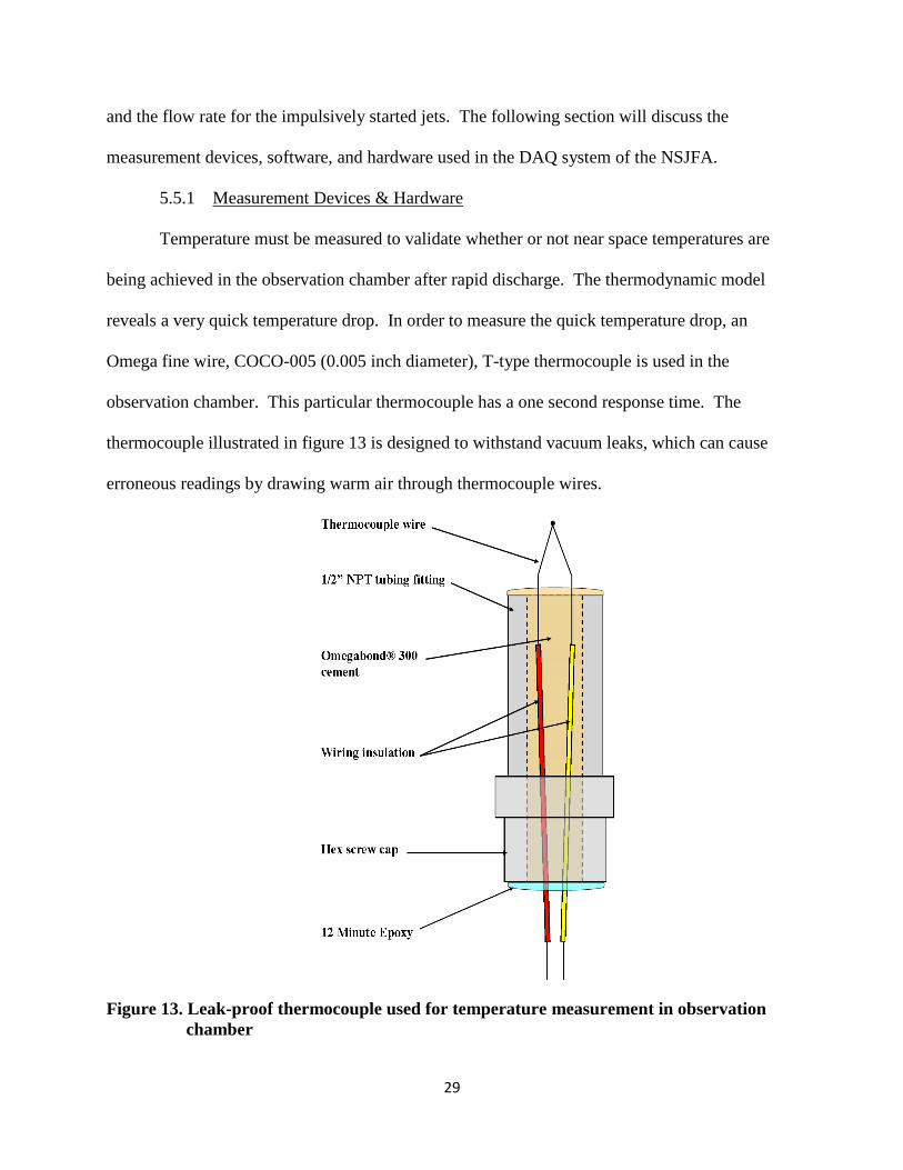
Temperature must be measured to validate whether or not near space temperatures are
being achieved in the observation chamber after rapid discharge. The thermodynamic model
reveals a very quick temperature drop. In order to measure the quick temperature drop, an
Omega fine wire, COCO-005 (0.005 inch diameter), T-type thermocouple is used in the
observation chamber. This particular thermocouple has a one second response time. The
thermocouple illustrated in figure 13 is designed to withstand vacuum leaks, which can cause
erroneous readings by drawing warm air through thermocouple wires.
Figure 13. Leak-proof thermocouple used for temperature measurement in observation
chamber

30
A ½-inch NPT steel tubing fitting was used as the housing for the T-type thermocouple. Wiring
insulation was used to separate the thermocouple leads inside of the steel fitting. The
thermocouple wires were led through the steel fitting and 12-Minute Epoxy was used to hold the
wires in place and serve as a seal. Once the 12-Minute Epoxy was hardened, the steel fitting was
filled with Omegabond® 300 cement, a thermally conductive, electrically insulating, one-part
cement designed for sealing and insulating thermocouples. A heat gun was used to cure the
cement at approximately 325ºF. Once dried, the Omegabond® 300 cement serves as a seal for
the thermocouple. Since the vacuum chamber does not experience extremely low temperatures,
an Omega, quick disconnect, K-type thermocouple (CASS-18(*)-12) fitted with a compression
fitting is sufficient for temperature measurement.
Pressure is an essential measurement in the observation chamber and vacuum chamber.
Since low temperatures are expected, it is necessary to use a pressure transducer that can
withstand harsh conditions. An Omega PX176 pressure transducer, shown in figure 14, was
chosen for measuring air pressure in both the observation chamber and vacuum chamber. The
Omega PX176 has an operating temperature from -55 to 105°C. It measures absolute pressure
and gives a 1-6 VDC output with a 9-20 VDC operational input power.

31
Figure 14. PX176 pressure transducer and wiring diagram (www.omega.com)
The wiring diagram shown above explains the connection of the PX176 pressure transducer.
The black wire is connected to the ground of the power supply while the red wire is connected to
a positive twelve volt power source. The white wire is connected to a data acquisition module
designed to read a voltage.
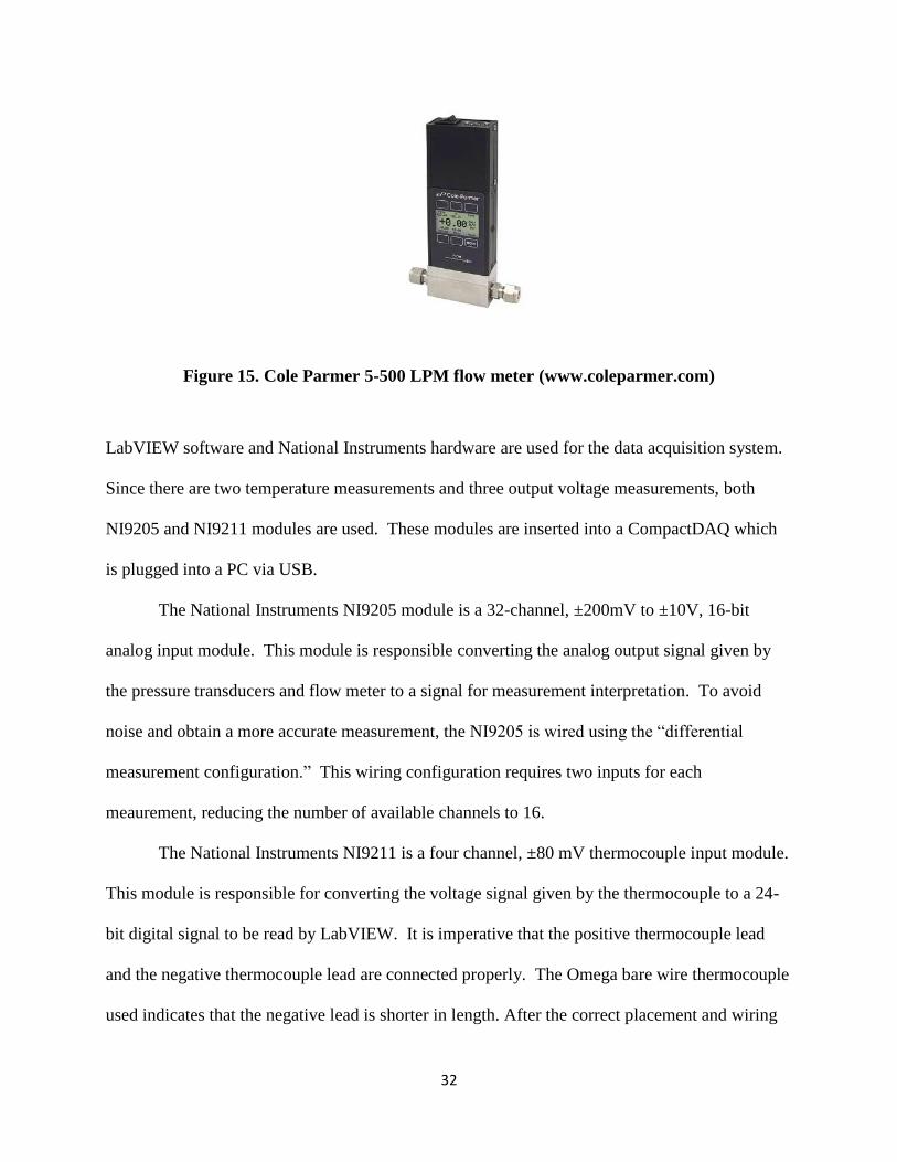
Since flow rates are of importance to this study, the volumetric flow rate of air through
the nozzle system is measured using a Cole Parmer K-32908-29 flow meter shown in figure 15.
This volumetric flow meter is highly accurate, can measure seventeen different gases, and
operates at a maximum pressure of 125 psi. This particular volumetric flow meter measures flow
between 0 and 500 liters per minute and gives a 0-5 VDC output with a 7-30 VDC operational
input power.
32
Figure 15. Cole Parmer 5-500 LPM flow meter (www.coleparmer.com)
LabVIEW software and National Instruments hardware are used for the data acquisition system.
Since there are two temperature measurements and three output voltage measurements, both
NI9205 and NI9211 modules are used. These modules are inserted into a CompactDAQ which
is plugged into a PC via USB.
The National Instruments NI9205 module is a 32-channel, ±200mV to ±10V, 16-bit
analog input module. This module is responsible converting the analog output signal given by
the pressure transducers and flow meter to a signal for measurement interpretation. To avoid
noise and obtain a more accurate measurement, the NI9205 is wired using the “differential
measurement configuration.” This wiring configuration requires two inputs for each
meaurement, reducing the number of available channels to 16.
The National Instruments NI9211 is a four channel, ±80 mV thermocouple input module.
This module is responsible for converting the voltage signal given by the thermocouple to a 24-
bit digital signal to be read by LabVIEW. It is imperative that the positive thermocouple lead
and the negative thermocouple lead are connected properly. The Omega bare wire thermocouple
used indicates that the negative lead is shorter in length. After the correct placement and wiring

33
of measurement devices is completed, DAQ system software is utilized in order to convert the
digital signals into a measurement value.
5.5.2 DAQ Software
The software used in this experiment for data acquisition is LabVIEW 8.6. LabVIEW,
short for Laboratory Virtual Instrumentation Engineering Workbench is a platform and
development environment for a visual programming language from National Instruments. It
converts a digital signal given by input modules into a measurement value for data processing.
This program allows users to create a custom data acquisition system, provided the correct
hardware is used.
LabVIEW is operated using a “block diagram” window and a “front panel” window. A
block diagram is created in LabVIEW to define what measurements are necessary for the
conversion of digital signals into measurement signals. The first step in creating a block diagram
is inserting a DAQ Assistant Express VI, shown in figure 16, into the block diagram window.
The DAQ Assistant Express VI allows the user to customize the data acquisition system. A user
can define the input signals given by the measurement devices, calibrate the measurement
devices if necessary, define a measurement scale to convert voltage to any unit, manipulate
sampling frequency and duration, and even displays a wiring diagram for measurement devices
to input modules if needed.

34
Figure 16. DAQ Assistant Express VI
Once placed, the properties of the DAQ Assistant Express VI are manipulated by right
clicking on the DAQ Assistant and choosing “Properties.” This opens a new DAQ assistant
window shown in figure 17.
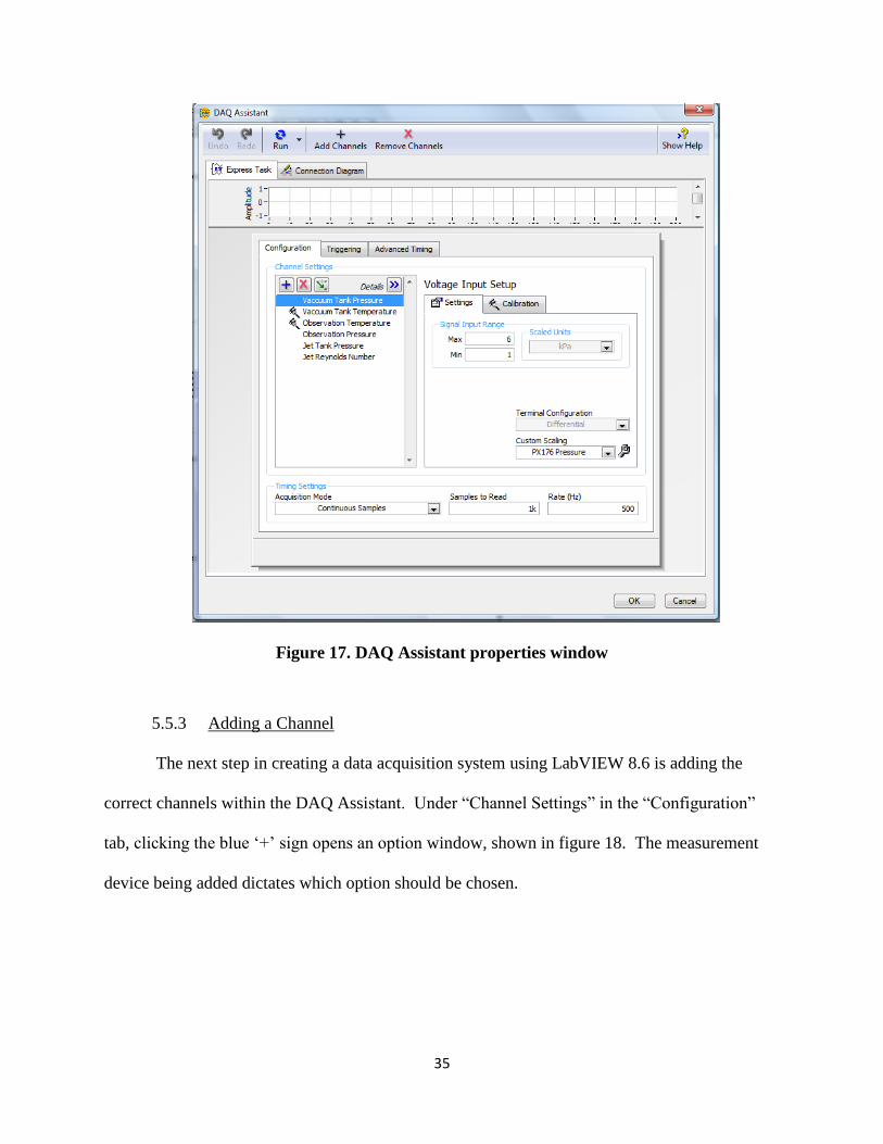
35
Figure 17. DAQ Assistant properties window
5.5.3 Adding a Channel
The next step in creating a data acquisition system using LabVIEW 8.6 is adding the
correct channels within the DAQ Assistant. Under “Channel Settings” in the “Configuration”
tab, clicking the blue „+‟ sign opens an option window, shown in figure 18. The measurement
device being added dictates which option should be chosen.

36
Figure 18. Input measurement option window
For a PX176 pressure transducer, “Voltage” must be chosen since the output signal from
this measurement device is 1 to 6 VDC. After clicking on “Voltage,” LabVIEW displays an
“Add Channels to Task” window shown in figure 19.

37
Figure 19. ‘Add Channels to Task’ window
Displayed in the “Add Channels to Task” window under “Supported Physical Channels”
are the available and correctly installed input modules, NI9205 and NI9211. Since the PX176
pressure transducers are connected to the NI9205 module, this option is selected. The
appropriate channel is selected depending on which channel the PX176 pressure transducer is
wired. After selecting the correct channel, the “OK” button is clicked and the user is returned to
the “DAQ Assistant Properties” window shown in figure 17.
Custom scaling must be created since the PX176 pressure transducer‟s output is a
voltage. The first step is to enter the maximum and minimum voltage output in the “signal input

38
range” shown below in figure 20. “Differential” should also be selected under “Terminal
Configuration” since this wiring configuration is used with the NI9205.
Figure 20. Maximum, minimum signal input ranges and terminal configuration selection.
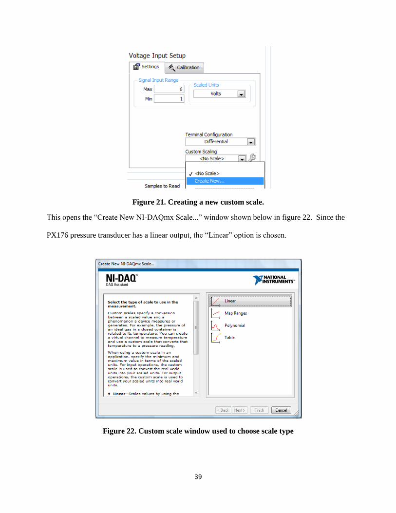
The next step is to click the drop-down window under “Custom Scaling” and selecting “Create
New” shown in figure 21.
39
Figure 21. Creating a new custom scale.
This opens the “Create New NI-DAQmx Scale...” window shown below in figure 22. Since the
PX176 pressure transducer has a linear output, the “Linear” option is chosen.
Figure 22. Custom scale window used to choose scale type

40
After choosing the “Linear” option, a new window will open giving the user the option to name
the custom scale. After naming the scale “PX176 Pressure,” the window shown in figure 23 is
opened, allowing the user to input the linear scale in algebraic form.
Figure 23. Custom scale window
Although basic linear algebra can be used to develop the equation for PX176 pressure as a
function of voltage, Microsoft Excel is utilized to create a plot of the voltage versus pressure,
insert a trend line, and display the trend line equation on the plot as seen in figure 24.

41
Figure 24. Pressure versus temperature plot used to obtain slope and y-intercept for PX176
25 psia pressure transducer scale
The slope and y-intercept are then put into the “Scaling Parameters.” Clicking „OK‟ enables the
DAQ to be built. This completes adding a PX176 pressure transducer to the DAQ system.
This process was followed to add each pressure transducer to the DAQ. Adding a thermocouple
is a very similar process. The thermocouples were calibrated using ice water and a room
temperature thermometer.
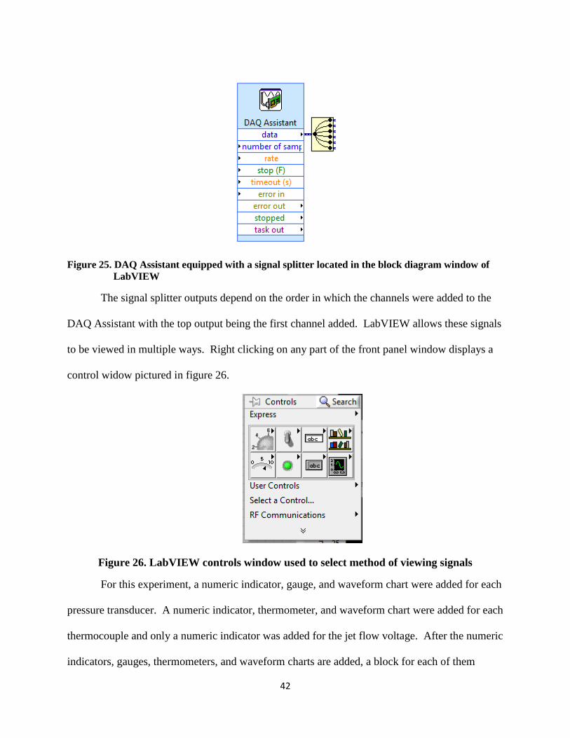
After adding all channels to the DAQ Assistant, the block diagram is revisited and a
“split signal” block, pictured in figure 25 is added.
y = 34.474x - 34.474
0
20
40
60
80
100
120
140
160
180
200
0 1 2 3 4 5 6 7
Pre
ssu
re (
kPa)
Voltage
42
Figure 25. DAQ Assistant equipped with a signal splitter located in the block diagram window of
LabVIEW
The signal splitter outputs depend on the order in which the channels were added to the
DAQ Assistant with the top output being the first channel added. LabVIEW allows these signals
to be viewed in multiple ways. Right clicking on any part of the front panel window displays a
control widow pictured in figure 26.
Figure 26. LabVIEW controls window used to select method of viewing signals
For this experiment, a numeric indicator, gauge, and waveform chart were added for each
pressure transducer. A numeric indicator, thermometer, and waveform chart were added for each
thermocouple and only a numeric indicator was added for the jet flow voltage. After the numeric
indicators, gauges, thermometers, and waveform charts are added, a block for each of them
43
appears in the block diagram window. Using the signal splitter, the signals are appropriately
“wired” to each of the blocks allowing the signal to be viewed in the front panel window.
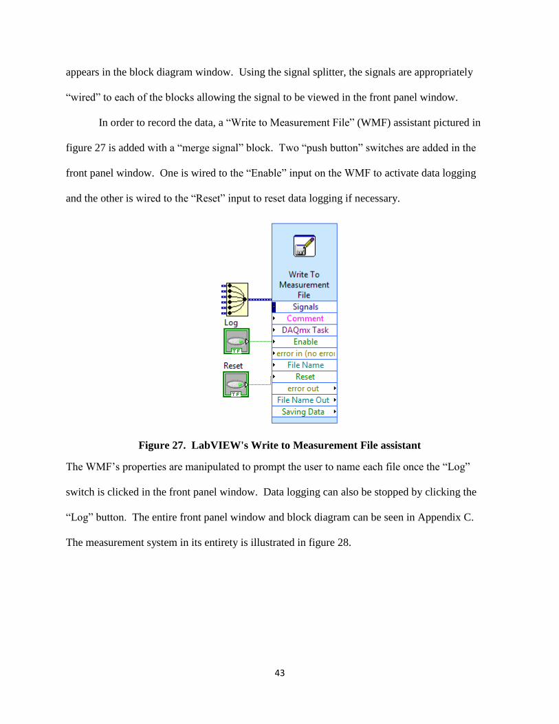
In order to record the data, a “Write to Measurement File” (WMF) assistant pictured in
figure 27 is added with a “merge signal” block. Two “push button” switches are added in the
front panel window. One is wired to the “Enable” input on the WMF to activate data logging
and the other is wired to the “Reset” input to reset data logging if necessary.
Figure 27. LabVIEW's Write to Measurement File assistant
The WMF‟s properties are manipulated to prompt the user to name each file once the “Log”
switch is clicked in the front panel window. Data logging can also be stopped by clicking the
“Log” button. The entire front panel window and block diagram can be seen in Appendix C.
The measurement system in its entirety is illustrated in figure 28.

44
Figure 28. Schematic of measurement system components
5.6 Shadowgraph System
A shadowgraph system is used to view the structure and behavior of the impulsively
started air jets. In a shadowgraph system, the linear displacement of the perturbed light is
measured (Goldstein 1996). A light source is used to create a beam of light directed toward a
concave mirror. The concave mirror directs the light source through a test section and projects a
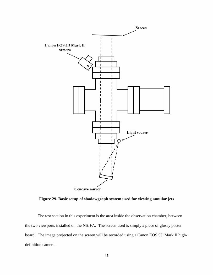
shadow image on a screen. The basic setup for the shadowgraph system used in this project is
pictured below in figure 29. The following section will discuss the components and setup of the
shadowgraph system used to view the annular jets.
45
Figure 29. Basic setup of shadowgraph system used for viewing annular jets
The test section in this experiment is the area inside the observation chamber, between
the two viewports installed on the NSJFA. The screen used is simply a piece of glossy poster
board. The image projected on the screen will be recorded using a Canon EOS 5D Mark II high-
definition camera.

46
The light source used in the shadowgraph system is a Phillips Lumiled LED light. The
LED provides an adequate amount of lighting for the projected image to be recorded on video
and analyzed. The light was installed on a piece of extruded aluminum and is equipped to be
adjustable in every direction by using Newport optical fine adjustment tools. The light intensity
is also adjustable by using resistor bank to alter the current supplied to the LED. The suggested
current for Phillips‟ Lumiled LEDs is 3500mA.
Figure 30. Electrical circuit for light source used in shadowgraph system
The concave mirror used in the shadowgraph system is 4.25” in diameter and is shown in
figure 31. This provides enough light area to shine through the circular viewports in order to
view the air jets. This mirror is mounted on a separate optical breadboard table and pieces that
make adjustments possible in every direction.

47
Figure 31. Concave mirror used in shadowgraph system
The 10-6” reducer flanges and viewports were removed from the observation chamber during
setup to make the viewing of the reflected parallel rays easier. The mirror used in this
experiment requires a distance between 45 and 60 inches from the light source in order to
properly straighten the parallel light rays. When properly adjusted, the diameter of the reflected
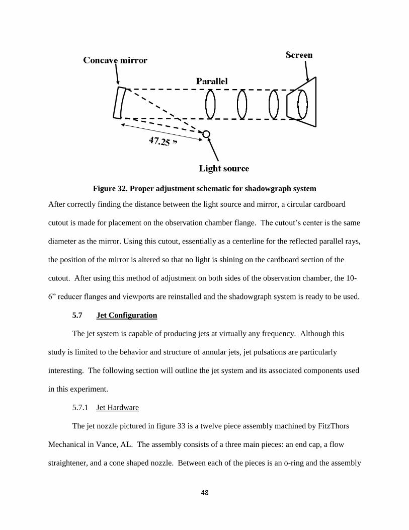
light should not change when the screen is moved away from the mirror as shown in figure 32.
This projected light is the same diameter of the mirror.
48
Figure 32. Proper adjustment schematic for shadowgraph system
After correctly finding the distance between the light source and mirror, a circular cardboard
cutout is made for placement on the observation chamber flange. The cutout‟s center is the same
diameter as the mirror. Using this cutout, essentially as a centerline for the reflected parallel rays,
the position of the mirror is altered so that no light is shining on the cardboard section of the
cutout. After using this method of adjustment on both sides of the observation chamber, the 10-
6” reducer flanges and viewports are reinstalled and the shadowgraph system is ready to be used.
5.7 Jet Configuration
The jet system is capable of producing jets at virtually any frequency. Although this
study is limited to the behavior and structure of annular jets, jet pulsations are particularly
interesting. The following section will outline the jet system and its associated components used
in this experiment.
5.7.1 Jet Hardware
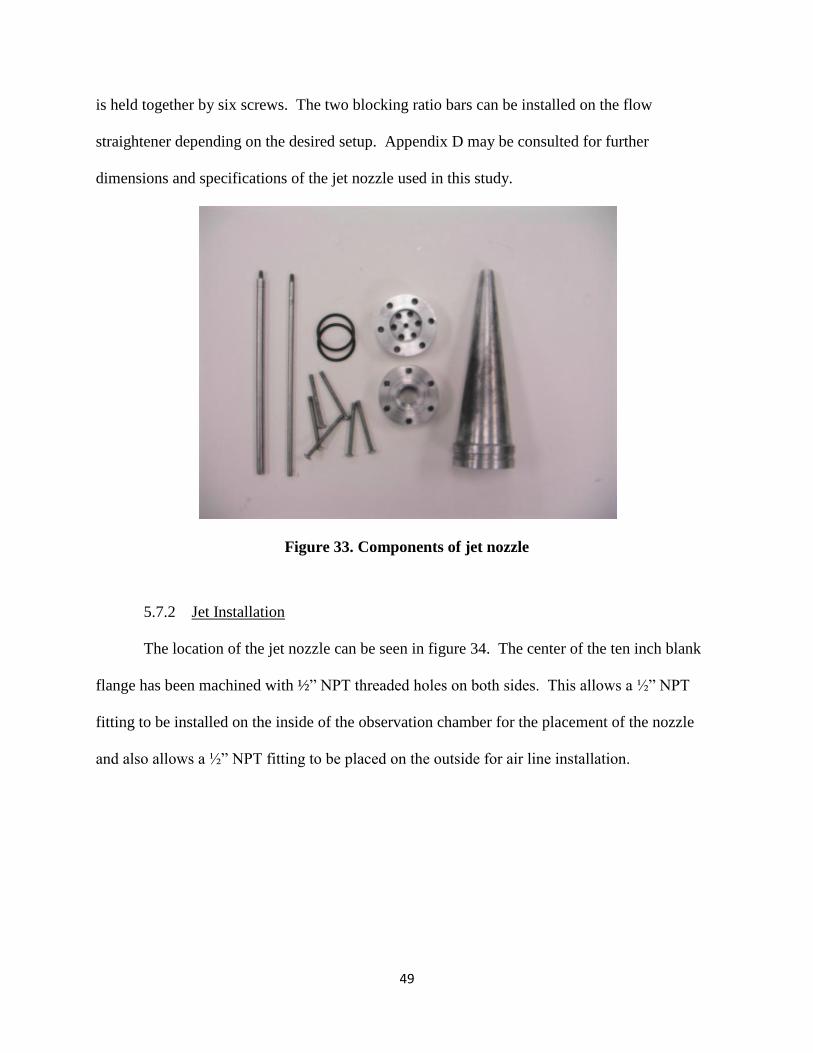
The jet nozzle pictured in figure 33 is a twelve piece assembly machined by FitzThors
Mechanical in Vance, AL. The assembly consists of a three main pieces: an end cap, a flow
straightener, and a cone shaped nozzle. Between each of the pieces is an o-ring and the assembly
49
is held together by six screws. The two blocking ratio bars can be installed on the flow
straightener depending on the desired setup. Appendix D may be consulted for further
dimensions and specifications of the jet nozzle used in this study.
Figure 33. Components of jet nozzle
5.7.2 Jet Installation
The location of the jet nozzle can be seen in figure 34. The center of the ten inch blank
flange has been machined with ½” NPT threaded holes on both sides. This allows a ½” NPT
fitting to be installed on the inside of the observation chamber for the placement of the nozzle
and also allows a ½” NPT fitting to be placed on the outside for air line installation.

50
Figure 34. Jet configuration inside observation chamber
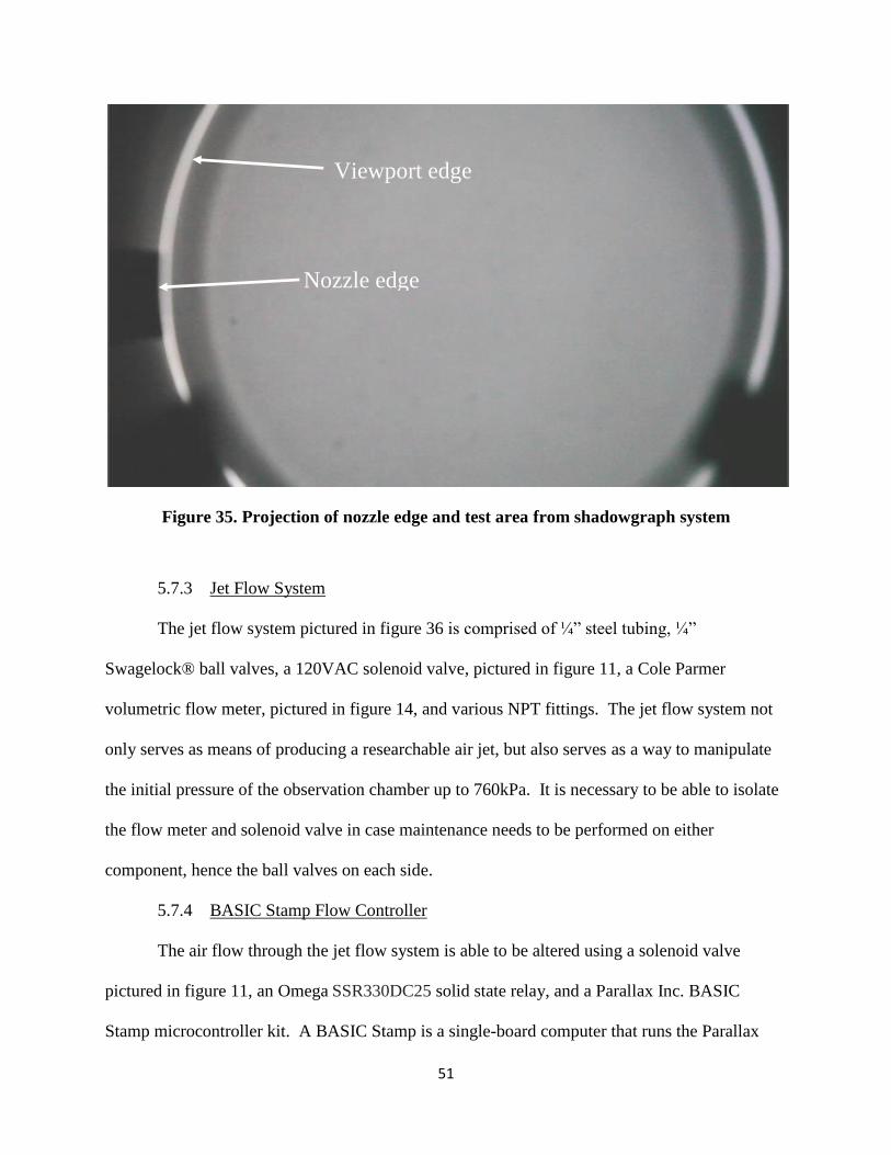
The nozzle is positioned inside of the observation so that the nozzle exit can be seen on
the edge of the projected shadow imagery, through the observation chamber viewports, as seen
below in figure 35.
51
Figure 35. Projection of nozzle edge and test area from shadowgraph system
5.7.3 Jet Flow System
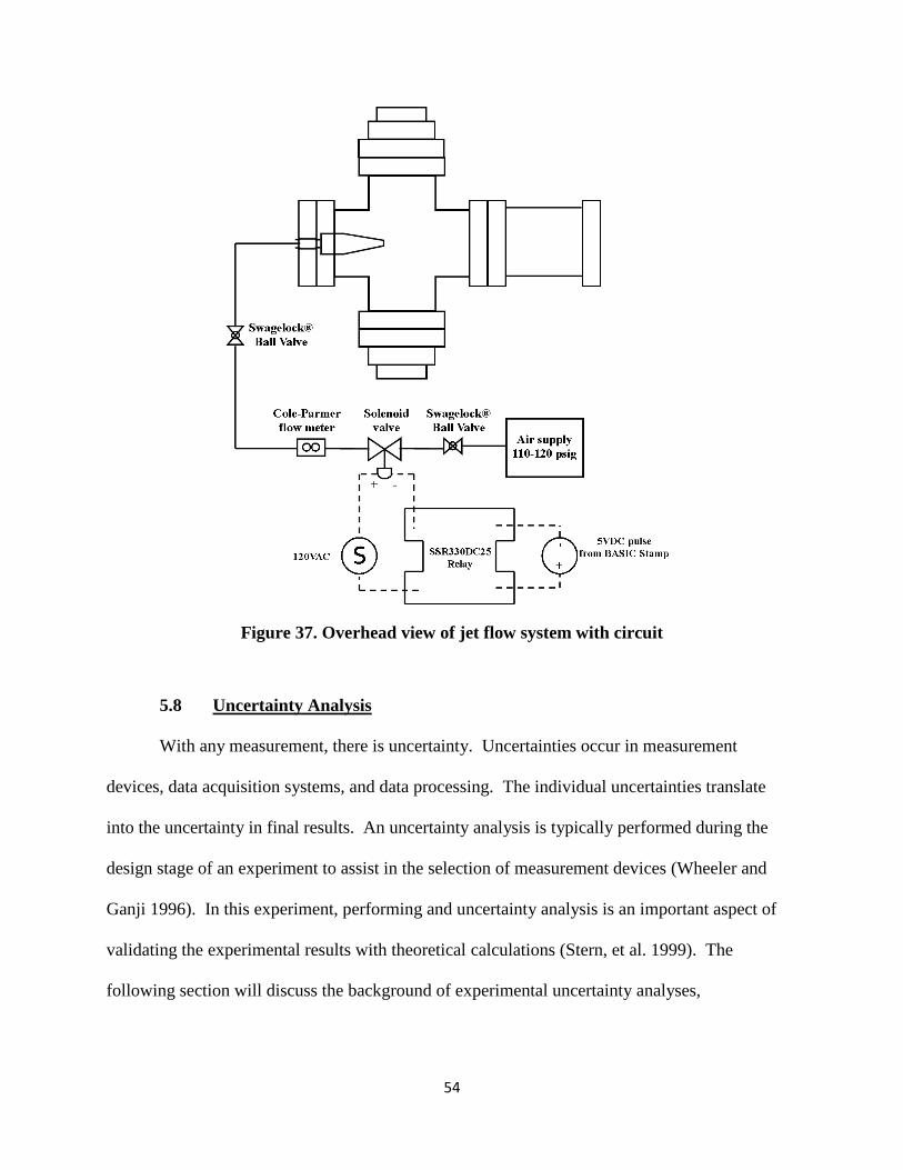
The jet flow system pictured in figure 36 is comprised of ¼” steel tubing, ¼”
Swagelock® ball valves, a 120VAC solenoid valve, pictured in figure 11, a Cole Parmer
volumetric flow meter, pictured in figure 14, and various NPT fittings. The jet flow system not
only serves as means of producing a researchable air jet, but also serves as a way to manipulate
the initial pressure of the observation chamber up to 760kPa. It is necessary to be able to isolate
the flow meter and solenoid valve in case maintenance needs to be performed on either
component, hence the ball valves on each side.
5.7.4 BASIC Stamp Flow Controller
The air flow through the jet flow system is able to be altered using a solenoid valve
pictured in figure 11, an Omega SSR330DC25 solid state relay, and a Parallax Inc. BASIC
Stamp microcontroller kit. A BASIC Stamp is a single-board computer that runs the Parallax
Viewport edge
Nozzle edge

52
PBASIC language interpreter in its microcontroller. The developer's code is stored in an
EEPROM (electrically erasable programmable read-only memory), which can also be used for
data storage. The PBASIC language has easy-to-use commands for basic I/O (About the BASIC
Stamp Microcontroller 2010). The BASIC Stamp circuitry communicates with the PC via USB
cable. For this experiment, a program was written to simply open and close the solenoid valve
for adjustable time durations. This program code is pictured in figure 36.
Figure 36. BASIC Stamp code used to initiate solenoid valve pulsation in jet flow system
(Pike 2010).
The program, written in BASIC Stamp Editor V2.2.4, places five direct current volts on
“PIN 0” for a desired duration of time. The “HIGH” command sets the specified pin to 1 (a
positive five volt level) and then sets its mode to output. The “PAUSE” delays the execution of
the next program instruction for the specified number of milliseconds. The “LOW” command
sets the specified pin to 0 (a zero volt level) and then sets its mode to output. The “GOTO”
command makes the BASIC Stamp execute the code that starts at the specified address location.

53
For this code, the specified address location is called “Main.” Since BASIC Stamp reads
PBASIC code from left-to-right, top-to-bottom, just like in the English language, the “GOTO”
command forces the BASIC Stamp to jump back to the first command “HIGH,” creating a
pulsating effect.
This voltage differential is wired from the pin location and ground on the BASIC Stamp
microcontroller to the positive and negative leads of the solid state relay. When the relay is
energized by the five volts from the BASIC Stamp, the circuit pictured in figure 37 is closed,
allowing the 120V solenoid valve to open for the specified number of milliseconds “FlashTm.”
Once the time duration has been reached, the five volt signal is turned off for the desired duration
of time, “PTm,” in milliseconds causing the solenoid valve to close. The jet flow system can be
seen in its entirety in figure 37.
54
Figure 37. Overhead view of jet flow system with circuit
5.8 Uncertainty Analysis
With any measurement, there is uncertainty. Uncertainties occur in measurement
devices, data acquisition systems, and data processing. The individual uncertainties translate
into the uncertainty in final results. An uncertainty analysis is typically performed during the
design stage of an experiment to assist in the selection of measurement devices (Wheeler and
Ganji 1996). In this experiment, performing and uncertainty analysis is an important aspect of
validating the experimental results with theoretical calculations (Stern, et al. 1999). The
following section will discuss the background of experimental uncertainty analyses,
55
measurement and experimental uncertainties related to this study, and the results from the
uncertainty analysis.
5.8.1 Measurement Uncertainty Background
The uncertainty of a measurement is using the root sum of the squares method, also
known as RSS (Wheeler and Ganji 1996). This method states that the uncertainty for a given
function can be calculated using the following equation (Wheeler and Ganji 1996).
(37)
5.8.2 List of Measurement Uncertainty
The first step to understanding the magnitude of experimental error is compiling a list of
measurement devices and their rated uncertainties. National Instruments has provided the
uncertainties for the thermocouples in the NI9211 manual. Using graphs and documentation
provided by the measurement device manufacturers, a table of uncertainties was constructed and
can be seen in table 3.
Table 3. List of measurement uncertainty
PX176 ±1% Repeatability
Linearity
Hysteresis
NI9211 2.5°C
K-type at -57°C
(w/Autozero)
3.0°C
T-type at -57°C
(w/Autozero)
Cole Parmer Flow
Meter
±0.8% Reading
±0.2% Full scale
±0.2% Repeatability
Nozzle Measurement ±1/32" Reading
Using this table, an uncertainty analysis can be performed for all values of tested temperature
and pressure.

56
5.9 Theoretical M-file
The thermodynamic model explained in section 3.4 was developed into an M-file for
theoretical calculations using MATLAB. This allows numerical values to be determined to
obtain the theoretical limitations of the observation chamber. After taking measurements, the
volume of the observation chamber and the vacuum chamber were calculated to be 0.0627m3 and
3.754m3 respectively.
Using these values with other miscellaneous constants, the MATLAB code is used to
calculate the theoretical capabilities of the NSJFA. A sample of the results for the vacuum
chamber initially at 10 kPa and the observation chamber at 101 kPa, both absolute
measurements, can be seen below in figure 38.
Figure 38. Sample pressure and temperature response from experimental pseudo-
algorithm m-file

57
These results justify the concept based on thermodynamic and fluid mechanic principles
as it can be seen that the result of an instantaneous discharge from a higher pressure to a lower
pressure produces a decrease in pressure as well as a decrease in temperature that eventually
translates into some finite steady state response. However, in a physical system, while the
pressure may remain the same during the steady state response, the temperature will rise
immediately after the lowest temperature is reached due to intruding heat transfer from the
surroundings. The next chapter will discuss how the thermodynamic model was utilized to
predict the capabilities of the NSJFA.

58
6. RESULTS AND DISCUSSION
6.1 Theoretical Discharge Model
The theoretical model discussed in section 4.9 was utilized to predict the capabilities and
limitations of the NSJFA. The experimental model was then tested to verify the results of the
theoretical model. A case matrix was made as a guideline for modeling multiple values of initial
pressure for theoretical and experimental models. For each case, the initial temperatures are
room temperature at approximately 22°C (298K). The following chapter will discuss the results
from the theoretical discharge models.
6.1.1 Case Matrix
For testing purposes, a case matrix was developed to determine the steady state value of
the observation chamber using the thermodynamic model. Referring to figure 1, it can be seen
that 216K is the lowest temperature in near space. It can also be seen that the lowest pressure
associated with near space is approximately 1.2 kPa. These boundaries are applied to the
development of the case matrix by running several preliminary tests using the thermodynamic
model.
Using the thermodynamic model, a realistic approach was taken to generate the upper and
lower bounds of initial pressures for the case matrix. In other words, initial pressures lower than
30 kPa were not tested since it was believed that these pressures would not create the low
temperatures and low pressures associated with near space in the experimental model. Testing

59
the experimental model would later prove this hypothesis true. For each case, the initial pressure
for the observation chamber was input into the m-file. Table 4 below is used as a case matrix for
the theoretical discharge model.
Table 4. Case matrix for theoretical discharge model
PA,init PB range
(kPa) (kPa)
110 100-10
100 90-10
90 80-10
80 70-10
70 60-10
60 50-10
50 40-10
40 35-5
30 25-1
6.1.2 Results
The value of the observation chamber‟s initial pressure determines the first tested value
of the vacuum chamber. Since a discharge from the observation chamber to the vacuum
chamber is necessary to create a temperature drop inside the observation chamber, only cases in
which PB < PA are considered. The resulting observation chamber pressure and temperature is
recorded in the column labeled “PA res” and “TA res” respectively. A sample of resulting
temperatures and pressures for one case can be seen in table 5.

60
Table 5. Sample case for various vacuum chamber pressure settings with observation
chamber kept at atmosphere
PA,init=110 kPa
PB PA res TA res
kPa kPa K
100 101.4 291.1
90 92.8 283.9
80 84.3 276.1
70 75.7 267.8
60 67.1 258.7
50 58.5 248.7
40 49.9 237.7
30 41.3 225.2
20 32.8 210.6
10 24.2 193.1
0 15.6 170.25
For each case listed in table 4, the results were plotted against the atmosphere curve from figure
2. The results can be seen below in figure 39.
Figure 39. Theoretical results of NSJFA plotted against atmosphere P-T curve
160
180
200
220
240
260
280
300
0 10 20 30 40 50 60 70 80 90 100 110
Tem
pe
ratu
re (
K)
Pressure (kPa)
Atmosphere
Pa,init=110 kPa
Pa,init=101 kpa
Pa,init=90 kPa
Pa,init=80 kPa
Pa,init=70 kPa
Pa,init=60 kPa
Pa,init=50 kPa
Pa,init=40 kPa
Pa,init=30 kPa

61
6.1.3 Discussion
After plotting results against the atmosphere curve and referencing the altitude chart in
Appendix A, it becomes obvious that the NSJFA is theoretically capable of creating temperatures
and pressures associated with altitudes for all of near space. Lower temperatures and lower
pressures are theoretically capable of being produced, but the conditions are inconsistent with a
near space environment. The next section will discuss the physical model of the system and how
the results compare to the theoretical results.
6.2 Experimental Discharge Model
The experimental model discussed in this thesis is tested against the results from
theoretical model. Using the vacuum pump, the vacuum chamber is evacuated to a certain
absolute pressure. Initially, the observation chamber was kept at atmospheric pressure,
approximately 100 kPa. The air compressor is turned on to supply 120 psi air to the lines
connected to the actuator‟s solenoid valves. After the vacuum tank pressure, observation
chamber pressure, and correct air pressure have been reached, the “Run” button in LabVIEW is
clicked following the “Log” switch being clicked. This prompts the user to name the file. After
naming the file, and clicking “OK,” the data starts being recorded. The three way switch is
turned on and the valve is opened. The system is allowed to stabilize before the valve is closed
and the “Log” switch is clicked again to stop data logging. The results are analyzed by opening
the saved file in Microsoft Excel and finding the lowest temperature reached in the observation
chamber.

62
6.2.1 Case Matrix
After a few preliminary tests, it became obvious that using the same case matrix as the
theoretical discharge model did not yield similar results. It was decided that since each discharge
was recorded, the testing of the experimental system could be less organized as the resulting
pressure from the previous test was used as the initial pressure of the vacuum chamber for the
next test. Having a more random study allowed more testing since the initial set points could be
reached in less time.
6.2.2 Results and Discussion
After completing approximately fifty preliminary tests, it became obvious that the
experimental model was not capable of creating the same results as the theoretical model when
given the same initial conditions. Although the temperature of the observation chamber did drop
for every test trial, it failed to reach the low temperatures associated with near space. The
preliminary test results can be seen below in figure 40.
Figure 40. Plot of experimental data from approximately fifty test runs
200
210
220
230
240
250
260
270
280
290
300
0 20 40 60 80 100 120
Tem
per
atu
re (
K)
Pressure (kPa)
Experimental Test Data
Atmosphere

63
Since the experimental discharge model is incapable of producing the temperatures associated
with near space, it was decided to study the annular jets for only the pressures associated with
near space. The next chapter will discuss the results from the annular jets tested at pressures
associated with high altitude.

64
7. JET TESTING
The annular jet nozzle discussed in section 4.7 was tested from pressures ranging from
0.5 kPa absolute to atmosphere. Referring to the standard atmosphere table in Appendix A, it
can be seen that this range covers all altitude pressures associated with near space. It is desirable
to have choked flow within the nozzle in order to establish a constant mass flow rate. Having a
constant mass flow rate allows the elimination of a variable within the experiment and allows an
analysis of the annular nozzles under the same flow conditions. The following section will
discuss the method used for testing the annular jets.
7.1 Testing Method
For each nozzle blocking ratio, the valve is left open and the entire system is evacuated
using the vacuum pump. The data logging is started using the DAQ system and LabVIEW and
video of the projected shadowgraph is recorded. The annular jet nozzle is pulsed on for three
seconds and off for three seconds until the NSJFA reached atmospheric pressure (~100 kPa).
Pulsating the jets, rather than a continuous flow, allows the air compressor to keep a constant
pressure air supply. After the NSJFA has reached atmospheric pressure, the video recording and
data logging is stopped.
The video is then uploaded into Adobe Premier Elements 4.0. Adobe Premier allows the
user to view and edit the video and take snapshots. The audio timeline was used in conjunction
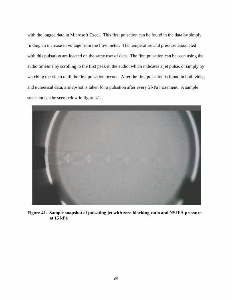
65
with the logged data in Microsoft Excel. This first pulsation can be found in the data by simply
finding an increase in voltage from the flow meter. The temperature and pressure associated
with this pulsation are located on the same row of data. The first pulsation can be seen using the
audio timeline by scrolling to the first peak in the audio, which indicates a jet pulse, or simply by
watching the video until the first pulsation occurs. After the first pulsation is found in both video
and numerical data, a snapshot is taken for a pulsation after every 5 kPa increment. A sample
snapshot can be seen below in figure 41.
Figure 41. Sample snapshot of pulsating jet with zero blocking ratio and NSJFA pressure
at 15 kPa

66
7.2 Results
After following this method discussed above and testing each nozzle setting from 0.5 kPa
to 100 kPa, the photos are cropped to show only the jet structure. Doing this allows multiple jet
structure pictures to be compiled for comparison. The contrast and brightness of the jet structure
picture compilation are altered to optimize the visualization of the jet structure. The results can
be seen below in figure 42.
Figure 42. Compilation of annular jet structures for NSJFA pressures between 0.5 kPa and
100 kPa

67
As expected, supersonic flow occurs after the exit of each nozzle. It can be assumed that
the Mach number is unity throughout the converging nozzle. It can be seen that upon fluid exit,
the jet structure changes as highlighted in section 3.1.2 of this thesis.
It is important to quantify the capabilities of the nozzle for each blocking ratio. The
motivation of this study is reliant on understanding the propulsion capabilities and jet structure
for possible use on a near space vehicle. The jet length is of particular importance since this will
determine the position and setup of the nozzle if used on a near space vehicle.
Figure 43. Visual jet length for nozzle with three blocking ratios
Using equation 5, the theoretical thrust was calculated for each blocking ratio for the
pressure range of the NSJFA. The nozzle exit pressure is calculated using equation 2. Since the
flow is choked, the velocity in the equation is theoretically equivalent to the speed of sound. The
maximum flow rate was calculated using equation 4. These solutions are for that of an ideal
nozzle flow explained in chapter 3 of this thesis. Figure 44 below shows the theoretical
capabilities of the nozzle for each tested blocking ratio.
0
10
20
30
40
50
60
70
80
90
100
0 10 20 30 40 50 60 70 80 90
NS
JF
A P
ress
ure
(k
Pa)
Visible Jet Length (mm)
Blocking Ratio = 0 Blocking Ratio = 0.5 Blocking Ratio = 0.75

68
Figure 44. Theoretical (isentropic) thrust capabilities
The actual thrust was calculated using values from measurement devices. The results from these
calculations can be seen below in figure 45.
Figure 45. Calculated experimental thrust for three nozzle blocking ratios
10
15
20
25
30
35
0 20 40 60 80 100
Th
rust
(N
)
NSJFA Pressure (kPa)
0 Blocking Ratio 0.5 Blocking Ratio 0.75 Blocking Ratio
4
6
8
10
12
14
16
0 20 40 60 80 100
Calc
ula
ted
Th
rust
(N
)
NSJFA Pressure (kPa)
Blocking Ratio = 0 Blocking Ratio = 0.5 Blocking Ratio = 0.75

69
The theoretical and actual thrust coefficient is also calculated using equation 5. The results of
the calculations can be seen below in figure 46. It can be seen that the theoretical thrust
coefficient is the same for all three blocking ratios.
Figure 46. Calculated experimental thrust coefficient
7.2.1 Resulting Experimental Uncertainty
The five measurements that are of particular importance to this experiment are the
volumetric flow of air in the jet system, the temperature of the observation chamber, the pressure
of the observation chamber, and the diameter measurement of the nozzle exit and blocking bar
diameter. Using geometry and the conservation of mass, equation 4 can be rewritten as
(38)
for a nozzle with any blocking ratio. The uncertainty percentage of the thrust is calculated using
equation 39. An expansion of the summation can be seen below.
0.300
0.350
0.400
0.450
0.500
0.550
0.600
0 10 20 30 40 50 60 70 80 90 100
Thru
st C
oe
ffic
ien
t
NSJFA Pressure
Blocking Ratio = 0 Blocking Ratio = 0.5 Blocking Ratio = 0.75
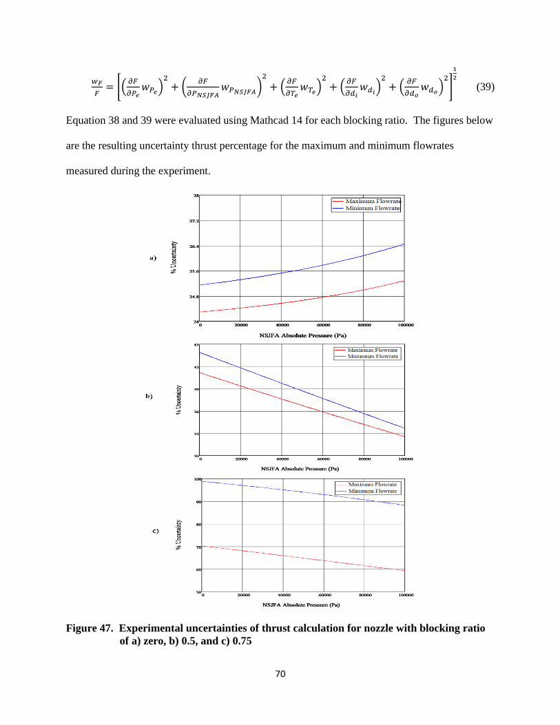
70
(39)
Equation 38 and 39 were evaluated using Mathcad 14 for each blocking ratio. The figures below
are the resulting uncertainty thrust percentage for the maximum and minimum flowrates
measured during the experiment.
Figure 47. Experimental uncertainties of thrust calculation for nozzle with blocking ratio
of a) zero, b) 0.5, and c) 0.75

71
For each blocking ratio, the uncertainty due to the measurements will fall between the graphed
lines. It can be seen that the uncertainty grows as the nozzle exit area is decreased. This is due
to the measurement uncertainty in the nozzle throat and blocking bar. As the diameter of the
blocking bar increases, the thrust area is decreased, leaving little room for error in the thrust
calculation. These figures should be referenced for future research with these nozzles.
7.3 Discussion
After compiling the results from the annular jets, it becomes apparent that there are
several different phenomena associated with the jet flow in each case. Shock diamonds are
clearly present in the nozzle setting without a blocking ratio. Referring to figure 3, it can be seen
that the presence of mach diamonds means that isentropic flow does not exist in that particular
flow. Since isentropic flow is also frictionless, an isentropic jet was unattainable during this
experiment. However, it can be seen that the documented jet results for the nozzle with no
blocking ratio are consistent with the converging-diverging nozzle exit relationships shown in
figure 3.
For each case, the flow is “overexpanded.” This means that the exit pressure, solved for
using equation 4, is less than the air supply pressure. The structure of an overexpanded jet can
be seen below in figure 48.
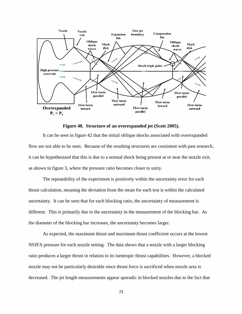
72
Figure 48. Structure of an overexpanded jet (Scott 2005).
It can be seen in figure 42 that the initial oblique shocks associated with overexpanded
flow are not able to be seen. Because of the resulting structures are consistent with past research,
it can be hypothesized that this is due to a normal shock being present at or near the nozzle exit,
as shown in figure 3, where the pressure ratio becomes closer to unity.
The repeatability of the experiment is positively within the uncertainty error for each
thrust calculation, meaning the deviation from the mean for each test is within the calculated
uncertainty. It can be seen that for each blocking ratio, the uncertainty of measurement is
different. This is primarily due to the uncertainty in the measurement of the blocking bar. As
the diameter of the blocking bar increases, the uncertainty becomes larger.
As expected, the maximum thrust and maximum thrust coefficient occurs at the lowest
NSJFA pressure for each nozzle setting. The data shows that a nozzle with a larger blocking
ratio produces a larger thrust in relation to its isentropic thrust capabilities. However, a blocked
nozzle may not be particularly desirable since thrust force is sacrificed when nozzle area is
decreased. The jet length measurements appear sporadic in blocked nozzles due to the fact that

73
the blocking bar is not perfectly symmetrical in the nozzle, particularly from errors during
machining. It can be seen that the maximum visible jet length occurs between 5 and 20 kPa for
each nozzle setting. These pressures correspond to altitudes ranging from approximately 12,000
to 20,000 meters. This length is particularly important to know. If this nozzle is installed on a
vehicle, it should be placed such that there is nothing obstructing the flow.

74
8. CONCULSION
8.1 Summary of Work
The purpose of this experiment was to design a near space jet flow apparatus that could
produce low temperatures and low pressures associated with near space, construct the near space
jet flow apparatus, and study annular jet structures in near space conditions
A pseudo-algorithm was developed to predict the theoretical capabilities of the designed
NSJFA and an m-file was created in MATLAB to solve for the final temperature and pressure of
the NSJFA. A case matrix was developed for input in the m-file, and the results were plotted
against the pressures and temperatures associated with near space. Theoretically, the NSJFA is
capable of producing temperatures and pressures associated with all altitudes of near space.
After constructing the NSJFA, setting up a data acquisition system, and installing the
necessary measurement devices, the NSJFA was tested. Upon completing fifty tests, it became
obvious that the physical model was incapable of producing the same results as the theoretical
model. It was decided to complete the remaining experiment with only the pressures associated
at high altitude.
After completing experiments for three blocking ratios of 0, 0.5 and 0.75, theoretical and
actual thrust calculations were performed to obtain a possible optimum nozzle setting. As
expected, the actual thrust is much smaller than the theoretical thrust because isentropic flow is
assumed in the theoretical calculations. Isentropic flow was not attainable in this experiment. In
order to theoretically obtain isentropic flow, the pressure at the nozzle exit must be equal to the

75
pressure of the NSJFA. This means that the supply pressure must equal 1.8939 times the NSJFA
pressure. The maximum thrust, as expected, occurs in a nozzle with no blocking ratio at 0.5 kPa.
While future research should be carried out on annular jets, it is not suggested to use a nozzle
with a blocking ratio because the small amount of thrust when compared to a nozzle with no
blocking ratio.
Based on this study, the following conclusions can be drawn:
Theoretical model predicted achievable temperatures and pressures associated
with all altitudes of near space.
NSJFA testing showed that theoretical results were not achievable.
It was decided to continue the jet study with only the pressures associated with
high altitude conditions.
The projected shadow imagery was recorded for structure analysis
Theoretical (isentropic) thrust and actual thrust calculations were performed for
nozzles with blocking ratios of 0, 0.5, and 0.75 using the measurements taken
with DAQ.
The maximum theoretical thrusts for a nozzle with blocking ratios of zero, 0.5 and
0.75 were calculated to be 31.9N, 23.93N and 14.13N respectively. All maximum
thrusts occur at an ambient pressure of 0.5kPa.
The maximum experimental thrusts for a nozzle with blocking ratios of zero, 0.5
and 0.75 were calculated to be 13.71 N, 10.53N and 7.59N respectively. All
maximum experimental thrusts occur at an ambient pressure of 0.5kPa.

76
The maximum experimental thrust coefficients for a nozzle with blocking ratios
of zero, 0.5 and 0.75 were calculated to be 0.430, 0.439, and 0.537 respectively.
All maximum thrust coefficients occur at an ambient pressure of 0.5 kPa.
Thrust coefficient results are in cohesion with previous research that involved a
gain in efficiency with some blockage of nozzle.
Maximum uncertainty for thrust and thrust coefficients for a nozzle with zero, 0.5,
and 0.75 blocking ratios are 26%, 44%, and 96% respectively.
8.2 Future Research
The NSJFA was designed to have a broad range of uses. Future research using the
NSJFA includes studying the pulsation of these air jets associated with this experiment as
discussed in section 2. Past research has been performed on pulsating jets and experiments have
shown that pulsed jets with no flow between pulses could produce up to 90% more thrust than
unpulsed jets (Krueger and Gharib 2005). A high speed camera has been purchased to capture
the impulsively started annular jet. Other future research may include finding an optimum
setting for each nozzle blocking ratio using compressible flow relationships and ideal nozzle
flow assumptions. Another future research project may include designing an aerospike for
insertion in the current nozzle.

77
9. REFERENCES
About the BASIC Stamp Microcontroller. 2010. http://www.parallax.com/tabid/295/Default.aspx
(accessed March 19, 2010).
Anderson, John D. Modern Compressible Flow. Third Edition. New York: McGraw-Hill, 2003.
Cao, Kang, and John Baker. "Application of Transient Network Models for Near Space." American
Institute of Aeronautics and Astronautics, 2008.
Cengal, Yunus A., and Michael A. Boles. Thermodynamics: An Engineering Approach. Sixth Edition. New
York: McGraw-Hill, 2008.
Colozza, Anthony. Initial Feasibility Assessment of a High Altitude Long Endurance Airship. Analex
Corporation, NASA, 2003.
Goldstein, Richard J., ed. Fluid Mechanics Measurements. Washington, DC: Taylor & Francis, 1996.
Handbook of Tables for Applied Engineering Science. 2nd Edition. CRC Press, 1973.
Kohle, Pankaj S., and Ajay K. Agrawal. "Density Measurements in a Supersonic Microjet Using Miniature
Rainbow Schlieren Deflectometry." AIAA 47, no. 4 (April 2009): 830-838.
Krueger, Paul S., and M. Gharib. "Thrust Augmentation and vortex Ring Evolution in a Fully Pulsed Jet."
AIAA Journal Vol. 43, no. No. 4 (2005).
Kruger, C. J.C. "KORF Hydraulics - Flexible fluid flow calculations." CACHE News, 1999: 11.
Lord, W. T. A Theoretical Study of Annular Supersonic Nozzles. Aeronautical Research Council, London:
Ministry of Aviation, 1961.
Mohensi, Kamran. "A formulation for calculating the translational velocity of a vortex ring or pair."
Bioinspiration & Biomimetics, 2006: S57-S64.
Munson, Bruce R., Donald F. Young, and Theodore H. Okiishi. Fundamentals of Fluid Mechanics. Fifth.
Hoboken: John Wiley & Sons, Inc., 2006.
National Instruments. What Is Data Acquisition? 2010. http://www.ni.com/dataacquisition/whatis.htm
(accessed June 13, 2010).

78
Nunn, Robert H. Intermediate Fluid Mechanics. New York, Washington, Philadelphia, London:
Hemisphere Publishing Corporation, 1989.
Olden, George W., David M. Lineberry, Christopher A.B. Linn, Brian D. Landrum, and Clark W. Hawk.
"Low-Cost Flow Visualization for a Supersonic Ejector." 41st AIAA/ASME/SAE/ASEE Joint Propulsion
Conference & Exhibit. Tuscon: AIAA, 2005.
Papamoschou, Dimitri, Andreas Zill, and Andrew Johnson. "Supersonic Flow Separation in Planar
Nozzles." Shock Waves 19, no. 3 (2008): 171-183.
Pasumarti, Ramya, Joseph Schulz, Jerry Seitzmanz, Jeff Jagoda, and Suresh Menon. "Large Eddy
Simulation of Pulsed Jets in High Speed Turbulent Cross." 48th AIAA Aerospace Sciences Meeting
Including the New Horizons Forum and Aerospace Exposition. Orlando: American Institute of Aeronautics
and Astronautics, 2010. 1-12.
Pike, Alston, interview by Nicholas Smith. Personal communication and training for BASIC Stamp
program Tuscaloosa, AL, (February 2010).
Scott, Jeff. Shock Diamonds and Mach Disks. April 17, 2005.
http://www.aerospaceweb.org/question/propulsion/q0224.shtml (accessed April 12, 2010).
Stephens, Buddy. Annular Nozzle Drawings. Mechanical Engineering Department, The University of
Alabama, Tuscaloosa.
Stern, Fred, Marian Muste, Maria-Laura Beninati, and William E. Eichinge. Summary of Experimental
Uncertainty Assessment Methodolgy with Example. IIHR Technical Report No. 406, College of
Engineering, The University of Iowa, Iowa City: Iowa Institute of Hydraulic Research, 1999.
Stoffel, James Robert. "Experimental and Theoretical Investigation of Aerospike Nozzles in a Hybrid
Rocket Propulsion System." 47th AIAA Aerospace Sciences Meeting Including The New Horizons Forum
and Aerospace Exposition. Orlando: AIAA, 2009.
Sutton, George P., and Oscar Biblarz. Rocket Propulsion Elements. 8th Edition. Hoboken: John Wiley &
Sons, Inc., 2010.
Tipler, Paul A, and Gene Mosca. Physics for Scientists and Engineers. 6th Edition. New York: W.H.
Freeman and Company, 2008.
Tomme, Lt. Col. Edward B. "The Paradigm Shift to Effects-Based Space: Near-Space as a Combat Space
Effects Enabler." Airpower Research Institue, 2005.

79
Wheeler, Anthony J., and Amhad R. Ganji. Introduction to Engineering Experimentation. Upper Saddle
River: Prentice Hall, Inc., 1996.
Williams, Keith, Michael J. Marcel, and John Baker. "Design of an Energy Management System for a Near
Space." American Institute of Aeronautics and Astronautics, 2007.
Witze, Peter O. "The Impulsively Started Incompressible Turbulent Jet." Combustion Application
Division, Sandia Laboratories, Livermore, California, 1980.
Young, Marcus, 2nd Lt Stephanie Keith, and Anthony Pancotti. "An Overview of Advanced Concepts for
Near-Space Systems." American Institute of Aeronautics and Astronautics (American Institute of
Aeronautics and Astronautics), 2009.
Zulkifli, Rozli, Kamaruzzaman Sopian, Shahrir Abdullah, and Mohd Sobri Takriff. "Experimental Study of
Flow Structures of Circular Pulsating Air Jet." American Journal of Engineering and Applied Sciences,
2009: 171-175.
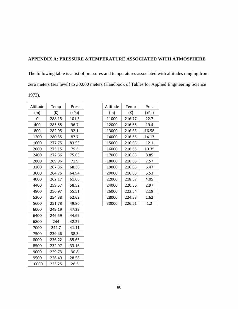
80
APPENDIX A: PRESSURE &TEMPERATURE ASSOCIATED WITH ATMOSPHERE
The following table is a list of pressures and temperatures associated with altitudes ranging from
zero meters (sea level) to 30,000 meters (Handbook of Tables for Applied Engineering Science
1973).
Altitude Temp Pres
Altitude Temp Pres
(m) (K) (kPa)
(m) (K) (kPa)
0 288.15 101.3
11000 216.77 22.7
400 285.55 96.7
12000 216.65 19.4
800 282.95 92.1
13000 216.65 16.58
1200 280.35 87.7
14000 216.65 14.17
1600 277.75 83.53
15000 216.65 12.1
2000 275.15 79.5
16000 216.65 10.35
2400 272.56 75.63
17000 216.65 8.85
2800 269.96 71.9
18000 216.65 7.57
3200 267.36 68.36
19000 216.65 6.47
3600 264.76 64.94
20000 216.65 5.53
4000 262.17 61.66
22000 218.57 4.05
4400 259.57 58.52
24000 220.56 2.97
4800 256.97 55.51
26000 222.54 2.19
5200 254.38 52.62
28000 224.53 1.62
5600 251.78 49.86
30000 226.51 1.2
6000 249.19 47.22 6400 246.59 44.69 6800 244 42.27 7000 242.7 41.11 7500 239.46 38.3 8000 236.22 35.65 8500 232.97 33.16 9000 229.73 30.8 9500 226.49 28.58 10000 223.25 26.5

81
APPENDIX B: THEORETICAL MODEL M-FILE
The following m-file was used to calculate the change in temperature and pressure of the NSJFA
during discharge.
clear all
clf
% INPUT DATA/INITIAL STATE
n = 5000; % -
tmax = 0.5; %s
Pao = 30; %kPa
Tao = 298.0; %K (77F)
Va = 0.06267 ; %m^3
Pbo = 5; %kPa
Tbo = 298.0; %K (77F)
Vb = 3.7535 ; %m^3
Dp = 0.0762; %m pipe diameter
Lp = 1.193; %m pipe length
Ap = 0.25*pi*Dp*Dp; %m^2 pipe diameter
%Constants
Rgas = 0.2870; % kJ/kgK gas constant for air
k = 1.4; % - ratio of specific heats for air
C = 1.0; % - assumed discharge coefficient
c1 = k*(2.0/(k+1.0))^((k+1.0)/(k-1.0));
c2 = (2.0*k)/(k-1.0);
c3 = (k-1.0)/k;
c4 = C*Ap;
c5 = ((k+1.0)/2.0)^(k/(k-1.0));
time = linspace(0.0,tmax,n);
dt = time(2)-time(1);
time(1) = 0.0;
Pa(1) = Pao;
Ta(1) = Tao;
Pb(1) = Pbo;
Tb(1) = Tbo;
%INITIAL MASS
ma(1) = (Pao*Va)/(Rgas*Tao); %kg
mb(1) = (Pbo*Vb)/(Rgas*Tbo); %kg
%INITIAL DENSITY
rhoa(1) = (ma(1)/Va); %kg/m^3

82
rhob(1) = (mb(1)/Vb); %kg/m^3
%INITIAL INTERNAL ENERGY
ua = 1.18900E-07*Tao^3 - 8.00883E-05*Tao^2 + ...
7.32878E-01*Tao - 1.78317E+00; %kJ/kg
ub = 1.18900E-07*Tbo^3 - 8.00883E-05*Tbo^2 + ...
7.32878E-01*Tbo - 1.78317E+00; %kJ/kg
Ua = ua*ma(1); %kJ
Ub = ub*mb(1); %kJ
i = 2;
while time(i-1)<tmax
pamd = Pa(i-1)*1000.0; % convert units to Pa
pbmd = Pb(i-1)*1000.0; % convert units to Pa
if(pamd/pbmd) >= c5;
% choked flow
mdota = c4*sqrt(rhoa(i-1)*pamd*c1); %kg/s
else(pamd/pbmd) < c5;
pd = 1.0 - (pbmd/pamd)^c3;
if pd<0.0
pd=0.0;
end
% non-choked flow
mdota = c4*rhob(i-1)*sqrt((pamd/rhoa(i-1))*c2*pd);
end
% tank mass at new time level
ma(i) = ma(i-1) - mdota*dt;
mb(i) = mb(i-1) + mdota*dt;
% specific enthalpy of gas leaving tank a
hea = 1.14610E-07*Ta(i-1)^3 - 7.36918E-05*Ta(i-1)^2 + ...
1.01724E+00*Ta(i-1) - 1.44501E+00; %kJ/kg
% Eulers method to integrate the internal energy
Ua = Ua - dt*mdota*hea;
Ub = Ub + dt*mdota*hea;
%calculate specific internal energy
ua = Ua/ma(i);
ub = Ub/mb(i);
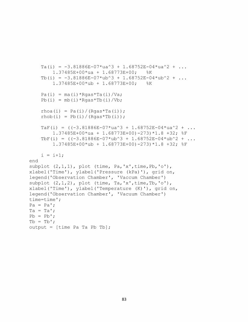
83
Ta(i) = -3.81886E-07*ua^3 + 1.68752E-04*ua^2 + ...
1.37485E+00*ua + 1.68773E+00; %K
Tb(i) = -3.81886E-07*ub^3 + 1.68752E-04*ub^2 + ...
1.37485E+00*ub + 1.68773E+00; %K
Pa(i) = ma(i)*Rgas*Ta(i)/Va;
Pb(i) = mb(i)*Rgas*Tb(i)/Vb;
rhoa(i) = Pa(i)/(Rgas*Ta(i));
rhob(i) = Pb(i)/(Rgas*Tb(i));
TaF(i) = ((-3.81886E-07*ua^3 + 1.68752E-04*ua^2 + ...
1.37485E+00*ua + 1.68773E+00)-273)*1.8 +32; %F
TbF(i) = ((-3.81886E-07*ub^3 + 1.68752E-04*ub^2 + ...
1.37485E+00*ub + 1.68773E+00)-273)*1.8 +32; %F
i = i+1;
end
subplot (2,1,1), plot (time, Pa,'x',time,Pb,'o'),
xlabel('Time'), ylabel('Pressure (kPa)'), grid on,
legend('Observation Chamber', 'Vaccum Chamber')
subplot (2,1,2), plot (time, Ta,'x',time,Tb,'o'),
xlabel('Time'), ylabel('Temperature (K)'), grid on,
legend('Observation Chamber', 'Vacuum Chamber')
time=time';
Pa = Pa';
Ta = Ta';
Pb = Pb';
Tb = Tb';
output = [time Pa Ta Pb Tb];
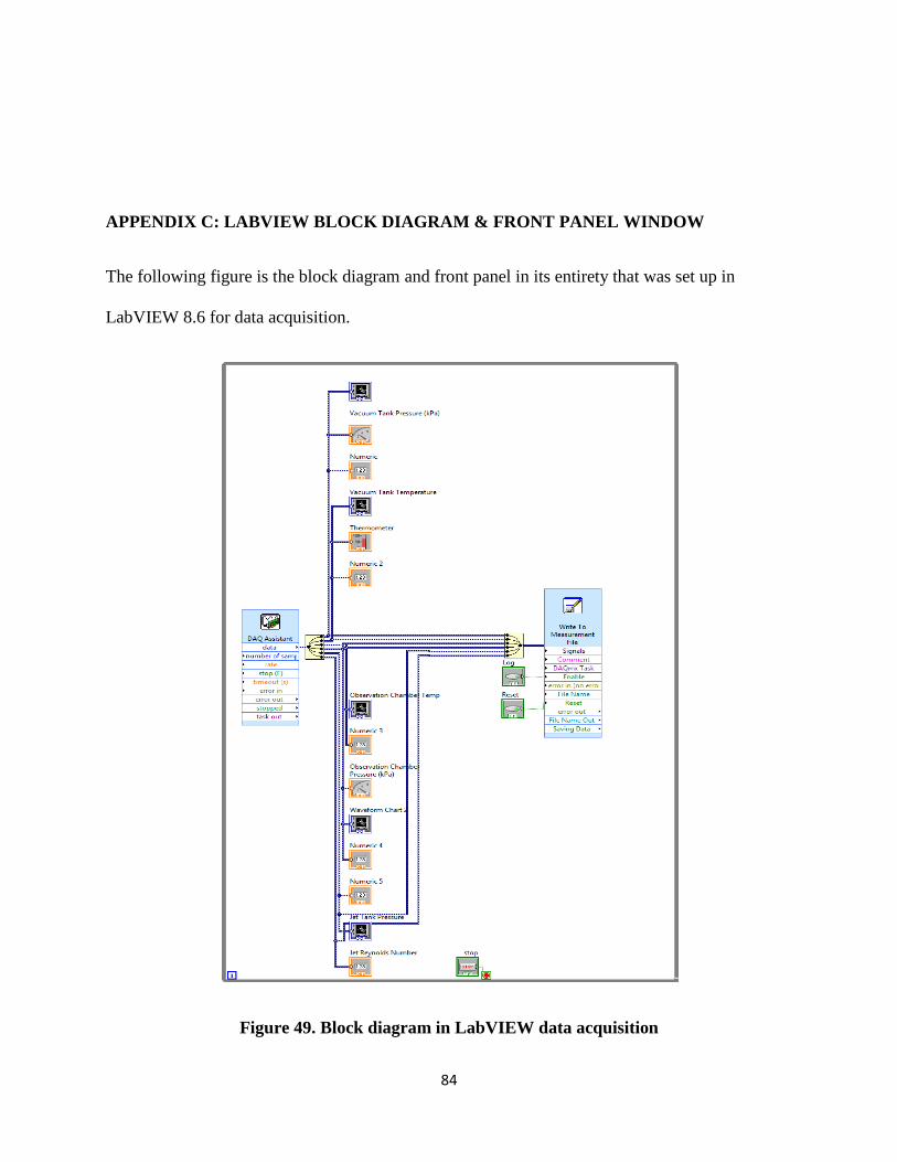
84
APPENDIX C: LABVIEW BLOCK DIAGRAM & FRONT PANEL WINDOW
The following figure is the block diagram and front panel in its entirety that was set up in
LabVIEW 8.6 for data acquisition.
Figure 49. Block diagram in LabVIEW data acquisition

85
Figure 50. Front panel window used in LabVIEW data acquisition
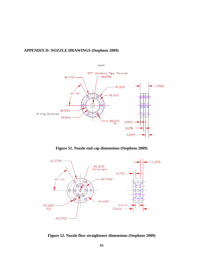
86
APPENDIX D: NOZZLE DRAWINGS (Stephens 2009)
Figure 51. Nozzle end cap dimensions (Stephens 2009)
Figure 52. Nozzle flow straightener dimensions (Stephens 2009)
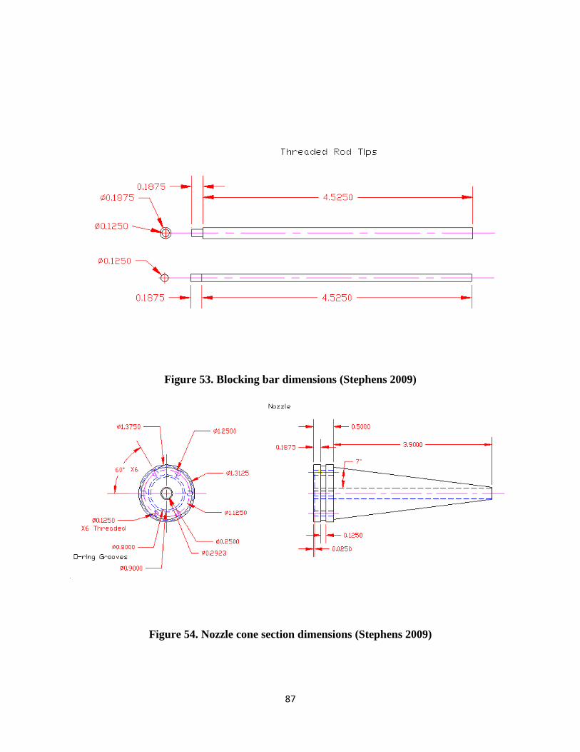
87
Figure 53. Blocking bar dimensions (Stephens 2009)
Figure 54. Nozzle cone section dimensions (Stephens 2009)