Development of a laser Doppler velocimeter for plastic … · Palavras-chave: Efeito de Doppler,...
143
Development of a laser Doppler velocimeter for plastic deformation monitoring INEGI – Institute of Mechanical Engineering and Industrial Management Ana Sofia de Freitas Alves Final Project / MIEM Dissertation FEUP Coordinator: Professora Doutora Ana Rosanete Lourenço Reis INEGI Coordinator: Doutor Paulo José da Silva Tavares INEGI Coordinator: Doutor Pedro Manuel Cardoso Teixeira Faculdade de Engenharia da Universidade do Porto Mestrado Integrado em Engenharia Mecânica June 2014
Transcript of Development of a laser Doppler velocimeter for plastic … · Palavras-chave: Efeito de Doppler,...
Development of a laser Doppler velocimeter for plastic deformation monitoring
INEGI – Institute of Mechanical Engineering and Industrial Management
Ana Sofia de Freitas Alves
Final Project / MIEM Dissertation
FEUP Coordinator: Professora Doutora Ana Rosanete Lourenço Reis
INEGI Coordinator: Doutor Paulo José da Silva Tavares
INEGI Coordinator: Doutor Pedro Manuel Cardoso Teixeira
Faculdade de Engenharia da Universidade do Porto
Mestrado Integrado em Engenharia Mecânica
June 2014


iii
ABSTRACT
With the emergence of new high speed forming techniques such as electromagnetic, electrohydraulic
or explosive forming the need arose to characterize materials for high speed deformation in
anticipation of an appreciable difference for properties in plastic deformation in such schemes. The
theme for this thesis arose from the scope of a FCT project to study the velocity of high speed forming
and trying to establish a relation between the velocity and the deformation capacity of material,
enabling the characterization of the materials.
This thesis has as main objective the development of a Doppler Effect velocimeter to subsequently
measure the deformation velocities on expansion test by magnetic impulse.
Throughout this work there was the need to study several interferometry techniques in order to better
understand the equipment and mastering the field of optical metrology as it relates to the topic of
thesis. As such two different interferometers were assembled: a Mach-Zehnder and a Michelson. It
was developed a Laser Doppler Velocimeter (LDV) based on Michelson Interferometer and it was
possible to measure velocities in the range of mm/s. It was also initiated the project to develop and
implement a Photon Doppler Velocimeter (PDV) capable of measuring velocities of several km/s. This
PDV was dimensioned in Optics and Experimental Mechanics Laboratory firstly to a Hopkinson bar
because this is the only equipment available in LOME capable of reaching velocities of m/s, in this
case 5 to 15 m/s approximately.
As a result of this work, a LDV was developed and it is being used in LOME to monitor the objects
movement, a PDV that is partially complete but already utilized to measure velocities and a portable
LDV with relatively adaptation and portability characteristics that the laboratory may now materialize.
Keywords: Doppler Effect, Photon Doppler Velocimeter, Laser Doppler Velocimeter, magnetic
impulse, Split Hopkinson Pressure Bar, interferometry, optical metrology.

iv
v
RESUMO
Com o aparecimento de novas técnicas de conformação plástica a altas velocidades, tais como
conformação plástica por impulso magnético, electro-hydraulic forming ou por explosão, surgiu a
necessidade de caracterizar os materiais para deformações a altas velocidades antecipando-se uma
diferença apreciável nas propriedades de deformação plástica nesses regimes. O tema para esta tese
surgiu do âmbito de um projeto FCT para estudar a velocidade da conformação plástica a alta
velocidade e tentar estabelecer uma relação entre a velocidade e a capacidade de deformação do
material, caracterizando deste modo os materiais.
Esta tese tem como objectivo principal o desenvolvimento de um velocímetro por efeito de Doppler
para posteriormente medir as velocidades de deformação em ensaios de expansão por impulso
magnético.
Ao longo deste trabalho houve a necessidade de estudar várias técnicas de interferometria de modo a
conhecer o equipamento e o domínio da metrologia óptica tal como se relaciona com o tema da tese.
Como tal foram montados dois interferómetros diferentes: um Mach-Zehnder e um Michelson. Foi
desenvolvido um Velocímetro Doppler por laser (LDV) com base no interferómetro de Michelson e
com ele foi possível medir velocidades da ordem dos mm/s. Foi igualmente iniciado o projeto de
desenvolvimento e implementação de um Photon Doppler Velocimeter (PDV) capaz de medir
velocidades de vários km/s. Este PDV foi dimensionado no Laboratório de Óptica e Mecânica
Experimental inicialmente para uma barra de Hopkinson, pois é o único equipamento existente no
LOME capaz de atingir velocidades na ordem dos m/s, no caso entre 5 e 15 m/s aproximadamente.
Como resultado deste trabalho, desenvolveu-se um LDV já utilizado no LOME para monitorizar o
movimento de objetos, um PDV, apesar de que ainda parcialmente completo apenas e que foi já
utilizado para medir velocidades e um protótipo para um LDV portátil com características de relativa
adaptação e portabilidade que o laboratório poderá agora concretizar.
Palavras-chave: Efeito de Doppler, Photon Doppler Velocimeter, Velocímetro Doppler por laser,
impulso magnético, Split Hopkinson Pressure Bar, interferometria, metrologia óptica.

vi
vii
ACKNOWLEDGEMENTS
In the first place I would like to thank to coordinator from Faculty of Engineering of the University of
Porto, Professor Ana Rosanete Reis for the encouragement and the opportunity to make this thesis in
INEGI – LOME.
A very special thank you to Doctor Paulo Tavares, my coordinator in LOME, for his support, valuable
advices, highest professionalism and human qualities that have set a precious example, which I follow,
and I aspire to attain someday.
Also to my coordinator Doctor Pedro Teixeira I would like to thank for the availability and useful
advices.
To Professor Mário Vaz I would like to thank the opportunity to make this project in Optics and
Experimental Mechanics Laboratory and for all the precious ideas throughout this work.
I would like to thank my colleague André Ferreira for all the help, availability and friendship
throughout this thesis. To Nuno Viriato I am grateful for all its availability and the help given so much
in the experimental part as in the project part and for all his sympathy and friendship. Finally I would
also like to thank Professor Luis Morão for help in deciding the subject of the thesis, the guidance
given during the thesis and throughout my academic career.
To Professor Geoffrey Taber, from Ohio State University, a special thanks for all the help on
developing the PDV and for all the advice given during this thesis.
A special thanks for all my colleagues at LOME, who have indeed been very supportive. In particular
to Ricardo Teixeira, Frederico Gomes and Paulo Pereira who have helped in different ways, and to all
those weren’t directly involved but had to withstand my enthusiasm doubts anyway.
Last, but in no way least important, my family and friends, always behind me and so supportive during
this project, I thank you all for all the help, care and concern.

viii

ix
Contents
1 INTRODUCTION ...........................................................................................................................1
1.1 Motivation ................................................................................................................................1
1.2 INEGI .......................................................................................................................................5
1.3 Objectives .................................................................................................................................6
1.4 Structure of the thesis ...............................................................................................................6
2 THEORETICAL BACKGROUND ................................................................................................7
2.1 The Doppler Effect ...................................................................................................................7
2.2 Optical Metrology ....................................................................................................................9
2.2.1 Optics ...............................................................................................................................9
2.2.2 Propagation of light ........................................................................................................15
2.2.3 The Superposition of waves ...........................................................................................15
2.2.4 Two-beam Interference ..................................................................................................16
2.2.5 Coherence .......................................................................................................................23
2.2.6 Two-beam Interferometers .............................................................................................26
2.2.7 Multiple-beam Interference ............................................................................................31
2.3 Heterodyne technique .............................................................................................................37
2.4 LDV ........................................................................................................................................38
2.5 PDV ........................................................................................................................................45
2.6 Fourier transform....................................................................................................................48
2.7 Split Hopkinson Pressure Bar ................................................................................................50
2.8 Electromagnetic forming ........................................................................................................51
3 EXPERIMENTAL WORK ...........................................................................................................53
3.1 The Mach-Zehnder Interferometer .........................................................................................53

x
3.2 LDV ....................................................................................................................................... 56
3.3 PDV ....................................................................................................................................... 62
4 DATA ANALYSIS....................................................................................................................... 69
4.1 Matlab® Code ....................................................................................................................... 69
4.2 Results from LDV ................................................................................................................. 70
4.2.1 LDV results for Low speed ........................................................................................... 70
4.2.2 LDV results for Normal speed ....................................................................................... 74
4.2.3 LDV results for high speed ............................................................................................ 77
4.2.4 Validation of the data .................................................................................................... 79
4.3 Results from PDV .................................................................................................................. 82
5 FUTURE WORK .......................................................................................................................... 87
5.1 Future Work ........................................................................................................................... 87
5.2 LDV Prototype ...................................................................................................................... 89
6 CONCLUSIONS .......................................................................................................................... 93
7 REFERENCES ............................................................................................................................. 95
8 ANNEXES .................................................................................................................................... 97
8.1 Annex A – Photo detector Data Sheet ................................................................................... 98
8.2 Annex B – Determination of the velocities of the micro-positioner .................................... 102
8.3 Annex C – Matlab® Code for LDV .................................................................................... 104
8.4 Annex D – Results from LDV ............................................................................................. 106
8.5 Annex E – Matlab ® code for PDV..................................................................................... 109
8.6 Annex F – Specifications from RIGOL ............................................................................... 110
8.7 Annex G – Specifications from laser diode ......................................................................... 111
8.8 Annex H – Specifications from detector ............................................................................. 114
8.9 Annex I – Specifications from fiber optical components .................................................... 117
8.10 Annex J – Specifications from EDFA Module amplifier .................................................... 119
8.11 Annex K – LDV Prototype .................................................................................................. 121
xi
LIST OF FIGURES
Figure 1.1 – (a) Typical part formed in a stamping or draw die with the die ring and without the punch;
(b) Section of tooling in a draw die [1] ....................................................................................................1
Figure 1.2 – Example of a FLC for aluminum [3] ...................................................................................2
Figure 1.3 – Quasi-static and dynamic forming limit curves [4] .............................................................3
Figure 1.4 – Scheme of dynamic ring expansion test to measure tensile stress-strain relations at high
strain rate [5] ............................................................................................................................................4
Figure 1.5 – Basic block diagram of the photonic Doppler velocimetry system [6] ................................5
Figure 2.1 – The Doppler effect [9] .........................................................................................................8
Figure 2.2 – Reflection and refraction of a light ray [13] ......................................................................10
Figure 2.3 – Flat mirror producing ghost reflections [13] ......................................................................12
Figure 2.4 – (a) Conventional planar beamsplitter; (b) Cube beamsplitter [13] ....................................12
Figure 2.5 – Schematic diagram showing the operation of an acousto-optic device [13] ......................13
Figure 2.6 – Interference fringes [15] ....................................................................................................18
Figure 2.7 – Young’s Interferometer [18] ..............................................................................................20
Figure 2.8 – Examples of wavefront-dividing interferometers: (a) Fresnel biprism; (b) Lloyd’s mirror;
(c) Michelson’s stellar interferometer [18] ............................................................................................21
Figure 2.9 – Michelson’s interferometer [18] ........................................................................................22
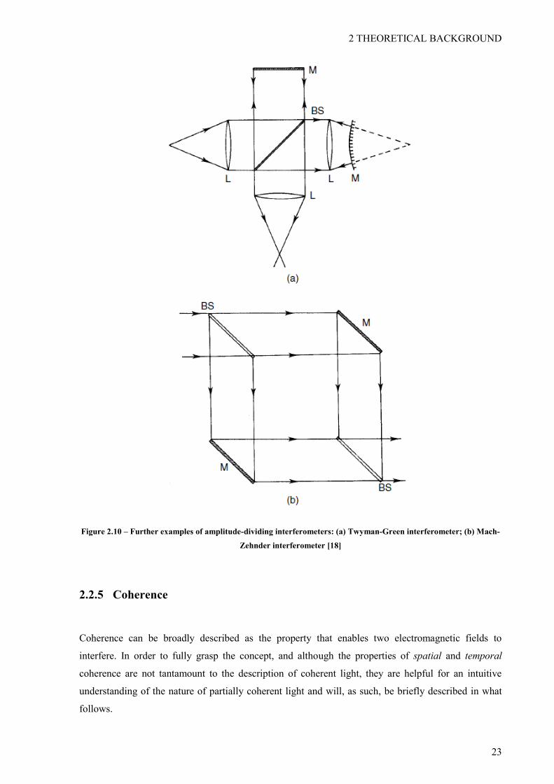
Figure 2.10 – Further examples of amplitude-dividing interferometers: (a) Twyman-Green
interferometer; (b) Mach-Zehnder interferometer [18] ..........................................................................23
Figure 2.11 – Wave trains of the partial waves [18] ..............................................................................25
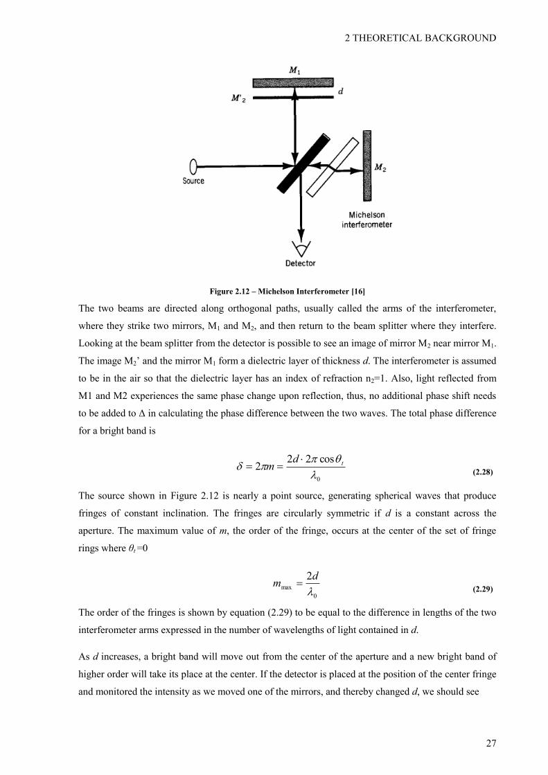
Figure 2.12 – Michelson Interferometer [16] .........................................................................................27
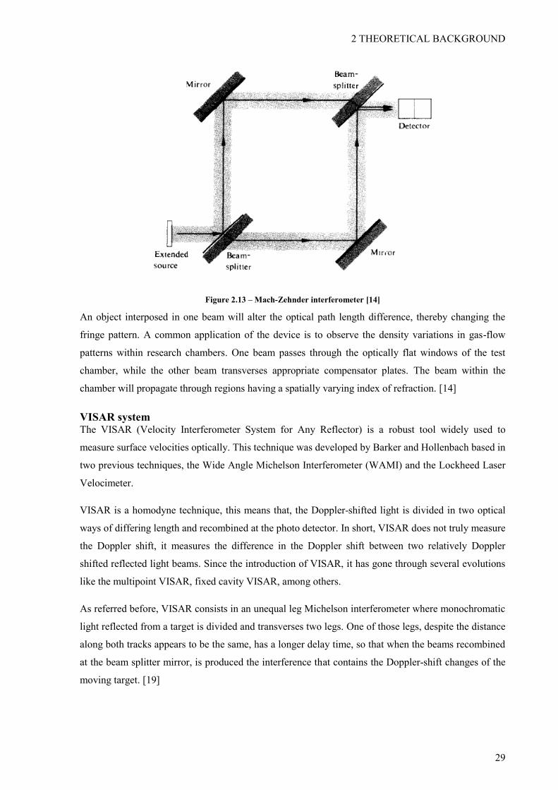
Figure 2.13 – Mach-Zehnder interferometer [14] ..................................................................................29
Figure 2.14 – VISAR Interferometer [20] ..............................................................................................30
Figure 2.15 – Multiple-beam interference from a parallel film [17] ......................................................31
Figure 2.16 – Plot of the fraction of transmitted light as a function of the optical path length [16] ......33
Figure 2.17 – Experimental arrangement of a Fabry-Perot interferometer [16] ....................................34
Figure 2.18 – Output fringes from a Fabry-Perot interferometer [16] ...................................................35
Figure 2.19 – Phase locked laser diode interferometer [29] ...................................................................37

xii
Figure 2.20 – Basic principle of the laser Doppler technique [9] .......................................................... 39
Figure 2.21 – System using one incident beam; (a) Dual-beam scattering configuration; (b) Reference-
beam configuration [9] .......................................................................................................................... 40
Figure 2.22 – Optical configuration for two incident waves; (a) dual-beam configuration; (b)
reference-beam configuration [9] .......................................................................................................... 41
Figure 2.23 – Vector relations relevant to determining the Doppler frequency [9] .............................. 42
Figure 2.24 – Generation of the interference structure of two homogenous waves. (a) (b) Electric field
strength of incident waves; (c) Superposition of electric fields; (d) Intensity [9] ................................. 43
Figure 2.25 – Signal origin for large particles [9] ................................................................................. 44
Figure 2.26 – Dual-beam laser Doppler Velocimetry [9] ...................................................................... 45
Figure 2.27 – Basic block diagram of the photonic Doppler Velocimetry system [30] ........................ 46
Figure 2.28 – Michelson interferometer VS simplified schematic of PDV [31] ................................... 47
Figure 2.29 – Components used in PDV [24] ....................................................................................... 48
Figure 2.30 – Scheme of a split Hopkinson pressure bar for tensile tests [35] ..................................... 51
Figure 2.31 – Scheme of Electromagnetic Forming process [7] ........................................................... 51
Figure 2.32 – Example of coil types commonly used on electromagnetic forming [7]......................... 52
Figure 3.1 – Mach-Zehnder scheme 1 ................................................................................................... 54
Figure 3.2 – Assembly of Mach-Zehnder scheme 1 .............................................................................. 54
Figure 3.3 – Mach-Zehnder scheme 2 ................................................................................................... 55
Figure 3.4 – Assembly of Mach-Zehnder scheme 2 .............................................................................. 55
Figure 3.5 – Diffracted beams from Mach-Zehnder scheme 2 .............................................................. 56
Figure 3.6 – LDV scheme 1................................................................................................................... 57
Figure 3.7 – M3 and driver from micro-positioner................................................................................ 57
Figure 3.8 – Assembly of LDV scheme 1 ............................................................................................. 58
Figure 3.9 – Signal from the PD for normal speed ................................................................................ 59
Figure 3.10 – Assembly of LDV scheme 2 with collimator .................................................................. 60
Figure 3.11 – Fringes obtained with the collimator ............................................................................... 60
Figure 3.12 – Fringes observed by the PD ............................................................................................ 61
Figure 3.13 – Scheme of the PDV applied in Hopkinson bar ............................................................... 63
Figure 3.14 – Assembly of the PDV ...................................................................................................... 64
Figure 3.15 – Detail of the circulator .................................................................................................... 64
Figure 3.16 – Detail of the connection between laser diode and circulator ........................................... 65
Figure 3.17 – Details of the probe and respective connections ............................................................. 65
Figure 3.18 – Detail of the detector ....................................................................................................... 66
Figure 3.19 – Moving surface adapted for Hopkinson Bar ................................................................... 66
Figure 3.20 – Final assembly of PDV in the Hopkinson bar ................................................................. 67
Figure 3.21 – Details of the adaptation of the PDV in the Hopkinson bar ............................................ 68
Figure 4.1 – a) Acquisition module NI 9234; b) Digital Oscilloscope Rigol DS6102 .......................... 69

xiii
Figure 4.2 – Scope image from the first measurement ...........................................................................83
Figure 5.1 – EDFA Module Mechanical Drawing .................................................................................88
Figure 5.2 – Detail of the amplifier inserted in the PDV .......................................................................88
Figure 5.3 – Final Scheme of the PDV adapted in Hopkinson bar ........................................................88
Figure 5.4 – Scheme of the portable LDV .............................................................................................89
Figure 5.5 – Scheme of the portable LDV .............................................................................................90
Figure 5.6 – External appearance of the LDV........................................................................................91
Figure 5.7 – Aspect of the LDV inside the box......................................................................................91
Figure 8.1 – Specifications from RIGOL DS6102 ...............................................................................110
Figure 8.2 – Calibration sheet of the laser diode ..................................................................................111
Figure 8.3 – Specifications of the Optical Circulator ...........................................................................117
Figure 8.4 – Specifications of the connector ........................................................................................117
Figure 8.5 – Specifications of the probe ..............................................................................................118

xiv

xv
LIST OF TABLES
Table 3.1 – Velocities from micro-positioner and respective expected frequency ................................58
Table 3.2 – Specifications from oscilloscope .........................................................................................62
Table 3.3 – Specifications of laser diode driver .....................................................................................62
Table 3.4 – Specifications of the optical components ............................................................................63
Table 4.1 – Resume of the obtained values ............................................................................................79
Table 8.1 – Measurements of the velocity from the micro-positioner .................................................102
Table 8.2 – Standard Deviation of values from Table 8.2 ...................................................................103

xvi

xvii
LIST OF GRAPHICS
Graphic 4.1 – Signal results from Low speed, (a) forward and (b) backward .......................................71
Graphic 4.2 – Signal results from Low speed, (a) forward and (b) backward with filter ......................73
Graphic 4.3 – Signal results from Normal speed, (a) forward ...............................................................75
Graphic 4.4 – Signal results from Normal speed, (a) forward with filter ..............................................76
Graphic 4.5 – Signal results from High speed, (a) forward....................................................................77
Graphic 4.6 – Signal results from High speed, (a) forward with filter ...................................................78
Graphic 4.7 – Frequency from the white light source ............................................................................81
Graphic 4.8 – Signal results from PDV for 1 MΩ .................................................................................83
Graphic 4.9 – Signal results from PDV for 50 Ω ...................................................................................84
Graphic 4.10 – FFT of the signal from PDV ..........................................................................................84

xviii
xix
LIST OF ABBREVIATIONS
AOM Acousto-Optic Modulator
BS Beamsplitter
CSV Common Separated Values
CW Continuous wave
EDFA Erbium Doped Fiber Amplifier
EMF Electromagnetic Forming
FCT Foundation for Science and Technology
FFT Fast Fourier Transform;
FLC Forming Limit Curve
LDV Laser Doppler Velocimetry;
LLNL Lawrence Livermore National Laboratory
LOME Optics and Experimental Mechanics Laboratory;
M Mirror
PD Photo detector
PDV Photon Doppler Velocimetry
SHPB Split Hopkinson Pressure Bar
STFT Short Time Fourier Transform
VISAR Velocity Interferometer System for Any Reflector

xx

1
1 INTRODUCTION
1.1 Motivation
Metal forming is a metalworking process of forming metal parts and objects through mechanical
deformation. In these processes the workpiece is reshaped without adding or removing material.
Forming operates on the principle of plastic deformation of each material where the physical shape of
a material is permanently deformed. This process is used in various applications like automobiles,
domestic appliances, aircraft, food and drink cans and also a host of other familiar products. The sheet
metal parts have the advantage that the material has a high elastic modulus and high yield strength so
that the parts produced can be stiff and have a good strength-to-weight ratio.
The conventional sheet metal forming process usually consists of a force that is applied into the sheet
against a die, with a determinate shape. There are various different operations using sheet metal
forming, such as, blanking and piercing, bending, stretching, hole extrusion, stamping or draw die
forming, deep drawing, among others.
Figure 1.1 – (a) Typical part formed in a stamping or draw die with the die ring and without the punch; (b) Section of
tooling in a draw die [1]

1 INTRODUCTION
2
In sheet metal forming there are two regimes of interest, concerning the properties of the material:
elastic and plastic deformation. For the conventional sheet metal forming, these mechanical
characteristics are well known due to the characterization of the materials commonly used in metal
forming.
The formability is limited, in most of the sheet metals, by the occurrence of localized necking. In order
to better understand the formability of each sheet metal Keeler and Backofen [2] reported that during
sheet stretching, the onset of localized necking required a critical combination of major and minor
strains. Consequently this concept was extended to drawing deformations by Goodwin [2] and the
resulting curve in principal strain space is known as the forming limit curve (FLC).
Figure 1.2 – Example of a FLC for aluminum [3]
These kinds of diagrams are usually obtained experimentally by stretching sheet metal samples over a
hemispherical punch. The principal strains are measured with the help of a regular or circular grid that
is electro-etched or printed onto the un-deformed blank, where the greater of the two principal strains
it is always positive, while the minor strain can be either negative or positive depending on the mode
of deformation. The left side of the FLC corresponds to a uniaxial tension and the right side of the
FLC is referred to biaxial tension therefore, the usual tests made to obtain the FLC are tensile tests for
uniaxial tension and Bulge-test or Nakajima for biaxial tension, among others.
In the automotive industry, environmental and economic matters have become some of the most
significant topics. The need of pollution reduction and costs saving, along with the increase of the
demands in performance, luxury and safety, is leading to the development of lightweight and more
energy efficient vehicles.
1 INTRODUCTION
3
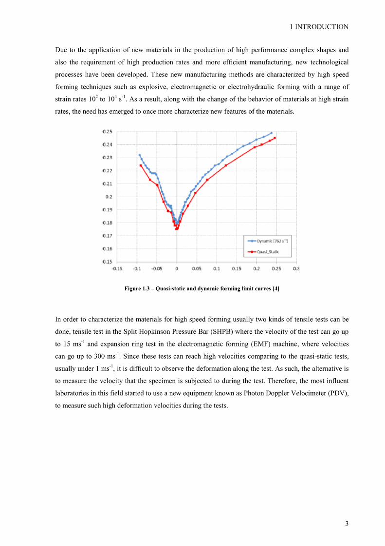
Due to the application of new materials in the production of high performance complex shapes and
also the requirement of high production rates and more efficient manufacturing, new technological
processes have been developed. These new manufacturing methods are characterized by high speed
forming techniques such as explosive, electromagnetic or electrohydraulic forming with a range of
strain rates 102 to 10
4 s
-1. As a result, along with the change of the behavior of materials at high strain
rates, the need has emerged to once more characterize new features of the materials.
Figure 1.3 – Quasi-static and dynamic forming limit curves [4]
In order to characterize the materials for high speed forming usually two kinds of tensile tests can be
done, tensile test in the Split Hopkinson Pressure Bar (SHPB) where the velocity of the test can go up
to 15 ms-1
and expansion ring test in the electromagnetic forming (EMF) machine, where velocities
can go up to 300 ms-1
. Since these tests can reach high velocities comparing to the quasi-static tests,
usually under 1 ms-1
, it is difficult to observe the deformation along the test. As such, the alternative is
to measure the velocity that the specimen is subjected to during the test. Therefore, the most influent
laboratories in this field started to use a new equipment known as Photon Doppler Velocimeter (PDV),
to measure such high deformation velocities during the tests.

1 INTRODUCTION
4
Figure 1.4 – Scheme of dynamic ring expansion test to measure tensile stress-strain relations at high strain rate [5]
Although the Hopkinson bar method is the dominant approach to characterize materials, it is a difficult
method to run in true uniaxial tension and the process of testing and data analysis is rather time
consuming. Moreover, as there are no standards in Hopkinson bar testing, it is difficult to obtain data
that is reproducible in detail from one lab to another. Therefore, the electromagnetically driven
expanding ring has been proposed as a test for high strain rate tensile testing by Niordson [5]. The
basic approach for the experiment is shown in Figure 1.4.
As a result, the need for measuring the velocity during the expanding ring tensile test is a consequence
from the necessity to prove the existing relation between the velocity or acceleration and the
deformation suffered during the tensile test of the ring.

1 INTRODUCTION
5
Figure 1.5 – Basic block diagram of the photonic Doppler velocimetry system [6]
PDV was developed in Lawrence Livermore National Laboratory (LLNL) by O. T. Strand [6]. This
velocimeter is based in a Laser Doppler Velocimeter (LDV) and along with the development of the
telecommunications industry, it was possible to create a relatively cheap velocimeter which is also
easy to operate, that can measure from mms-1
to kms-1
. PDV uses fiber optics technologies and is
limited only by the bandwidth of the electrical test components.
As part of a new project by INEGI – CETECOP / LOME, the need arose to develop a PDV to measure
velocities of expanding ring tests made in the electromagnetic forming machine in order to
characterize the materials AL 6082 T6 and AZ 31 B – H24, aluminum and magnesium alloys
respectively. The need to develop the PDV instrument is mostly due to the fact that this is a relatively
new technology and therefore only a few laboratories in the world have it. None of these are located in
Portugal or anywhere near, therefore preventing the possibility of partnerships between nearby
laboratories. This project arises from a FCT project grant: EXPL/EMS-TEC/2419/2013. [1, 2, 4-8]
1.2 INEGI
INEGI (Institute of Mechanical Engineering and Industrial Management) was started in 1986, from the
Department of Mechanical Engineering and Industrial Management (DEMEGI) of the Faculty of
Engineering of University of Porto and is an interface Institute between University and Industry,
oriented to the activities of research and development, innovation and technology transfer. It is
considered an active agent playing a significant role in the development of the Portuguese industry,
and in the transformation of its competitive model.
The Optics and Experimental Mechanics Laboratory (LOME) is an operational division of INEGI
focused on research activities for design, validation and inspection of structures and mechanical
components. It is composed by an interdisciplinary group of researchers with expertise in multiple

1 INTRODUCTION
6
sensing technologies for structural monitoring, advanced manufacturing processes for metallic
structures, structural integrity, multi-body modeling, optics and laser metrology, experimental
mechanics, biomechanics, among others. These activities have been conveniently grouped into four
distinctive areas: Non-destructive Testive or Inspection (NDT / NDI), experimental Mechanics and
New Technologies, Structural Health Monitoring, and, Biomechanics.
1.3 Objectives
The objective of this work was the development and implementation of Laser Doppler Velocimeters
and the Photon Doppler Velocimeter and also to develop a LDV to measure low velocities and make a
portable prototype to be used in LOME for innumerous applications requiring velocities
measurements.
A second objective of the current work was the start of the development of a PDV to be applied in the
electromagnetic forming machine, to measure velocities in the expanding ring tests. Since the fastest
tensile test machine existing in LOME is the SHPB, it was deemed appropriate to study a way to apply
the LDV and the PDV in the SHPB.
1.4 Structure of the thesis
In a way to complete all the proposed objectives, this thesis was divided in 6 chapters. This is the first
chapter, the introduction and motivation for this thesis. Chapter 2 presents the theoretical background
for the development of PDV. This chapter contains some basic background on Optics and Optical
Metrology, all the concepts that made possible the PDV and how the processing data is made. It also
presents the diverse applications and also the advantages and disadvantages of the technology.
Chapter 3 and Chapter 4 describe all the work done during the development of a PDV. In Chapter 3 all
the experimental work from the development of a LDV through to the first low-velocity measurements
with a different LDV setup and to the setup and deployment of a PDV and its application to
measurements in the Hopkinson Bar, is described. In Chapter 4 all the performed data analysis is
presented both for the LDV and for the PDV and a brief explanation of how the developed Matlab ®
program for data analysis works.
Chapter 5 is divided in two sections. The first section refers the foreseen future work, where the work
that is likely to be done in the future is described. In the second section, a proposal for a portable LDV
prototype is presented.
Finally in Chapter 6, all the conclusions reached throughout the thesis are written.

7
2 THEORETICAL BACKGROUND
Since the LDV is based in optics and interferometric techniques, there has been the need to study some
basics of Optics and Optical Metrology. This chapter explains all the theoretical background needed to
understand and develop a LDV and later on, a PDV.
In this chapter, the phenomenon behind the measurement of velocity with these technologies, known
as the Doppler Effect, is first explained. Afterwards, there is a summary about the basics of optics, the
most commonly used components, some interferometry techniques and the different interferometers
used in most optical laboratories. Another technique used in the measurement of velocities is the
heterodyne technique, also explained therein.
Finally, the LDV and PDV techniques are covered as well as the data analysis is made and all the
mathematics behind the data analysis of the results, such as the Fast Fourier Transform (FFT), an
algorithm used in the most daily electronic equipment.
2.1 The Doppler Effect
Although there seems to be no historical account of the popular perception of the effect, it is easy to
assume the Doppler Effect had been notice before, probably since antiquity. Johann Christian Doppler
proposed in 1846 an explanation to an observable effect where the frequency of waves emitted from a
moving object is shifted from the original frequency. Since then, the Doppler shift phenomenon has
been realized in many applications extending from weather and aircraft radar systems to the
measurement of blood flow in unborn fetal vessels. The Doppler Effect became central to most of the
interferometric techniques for measuring velocities.
According to the description of the effect, light shone by an observer against an object moving toward
him will be reflected with a higher frequency.
The effect is readily observable irrespective of the movement of either the transmitter or the receiver
of the electromagnetic radiation.

2 THEORETICAL BACKGROUND
8
Figure 2.1 illustrates the principle of the Doppler Effect.
Figure 2.1 – The Doppler effect [9]
An electromagnetic wave originating from a moving transmitter with a velocity vp and a frequency fp is
apparently compressed for an observer standing in the direction of the movement and apparently
expanded in the opposite direction. This results in a change of wavelength or frequency described as,
c
ev
fcf
c
ev
prp
p
r
rp
prp
pr
1
,
(2.1)
The noticed wavelength λp and the frequency fp of a moving receiver with relative velocity vp with
respect to the stationary transmitter is given by
l
lpp
p
lpp
l
p
evff
c
ev
1,
1
(2.2)
If the transmitter and the receiver are moving, then the Doppler Effect is invoked twice and the noticed
frequency at a stationary receiver for a stationary laser and for light scattered from a moving particle
becomes (| | )

2 THEORETICAL BACKGROUND
9
c
eevff
prlpp
lr
)(1 (2.3)
In other words, the Doppler Effect occurs when a source S emits waves at a frequency v and
wavelength λ to an observer O, the frequency being observed as f’ and the wavelength as λ’ if the
source S’ moves during the transmission.
It is possible to say that the Doppler Effect consists of a change of the observed frequency, although it
is, in essence, a relativistic effect, observed by the receiver and not by the source. [9-12]
2.2 Optical Metrology
Optical Metrology is the subject which covers all sort of measurements made with light, regardless of
the wavelength. Optical Metrology is usually separated into Radiometry and Photometry, depending
on the fact the wavelength being used falls inside the 360 – 830nm limit of the visible part of the
electromagnetic spectrum, as established by the International Commission on Illumination .(CIE;
Commission Internationale de l’Éclairage).
In the following, a brief introduction to Optics and interferometers is exposed, that enables the readers
less acquainted with the subject to follow the work in this thesis, on Laser and Photon Doppler
Velocimeters
2.2.1 Optics
Light is one form of electromagnetic radiation, the many categories of which make up the
electromagnetic spectrum. Electromagnetic radiation, which transports energy from point to point at
the velocity of light, can be described in terms of both wave and particle “pictures” or “models”. This
is the famous “wave-particle” duality of all fields or particles in our model of the universe. In the
electromagnetic-wave picture, waves are characterized by their frequency ν, wavelength λ, and the
velocity of light c, which are related by .
A propagating electromagnetic wave is characterized by a number of field vectors, which vary in time
and space.
For a complete description the polarization state of the wave must also be specified. Linearly polarized
waves have fixed directions for their field vectors, which do not re-orient themselves as the wave
propagates. Circular or elliptically polarized waves have field vectors that trace out circular or elliptic

2 THEORETICAL BACKGROUND
10
helical paths as the wave travels along. In the particle counterpart picture, electromagnetic energy is
carried from point to point as quantized packets of energy called photons.
Optical materials have refractive indices that vary with wavelength. This phenomenon is called
dispersion. It causes a wavelength dependence of the properties of an optical system containing
transmissive components. The change of index with wavelength is very gradual, and often negligible,
unless the wavelength approaches a region where the material is not transparent. A description of the
performance of an optical system is often simplified by assuming that the light is approximately
monochromatic, i.e., contains only a small spread of wavelength components. [13]
Reflection and Refraction
The phenomena of reflection and refraction are most easily understood in terms of plane
electromagnetic waves – those in which the direction of energy flow is unique.
When light is reflected from a plane mirror, or the planar boundary between two media of different
refractive index, the angle of incidence is always equal to the angle of reflection, as shown in Figure
2.2. This is the fundamental law of reflection.
Figure 2.2 – Reflection and refraction of a light ray [13]

2 THEORETICAL BACKGROUND
11
For the light ray that crosses the boundary between two media of different refractive indices, the angle
of refraction θ2 is related to the angle of incidence θ1 by Snell’s law:
1
2
2
1
sin
sin
n
n
(2.4)
This result is further modified if one or both of the media is anisotropic. [13]
Optical Components
A few of the most common components are described in what follows in simple grounds, because
these components were used most often during the experimental work. The reader is referred to
conventional Optics literature for further details about each of this element.
Mirrors – When light passes from one medium to another of different refractive index, there is always
some reflection, so the interface acts as a partially reflecting mirror. By applying an appropriate single-
layer or multilayer coating to the interface between the two media, the reflection can be controlled so
that the reflectance has any desired value between 0 and 1. If no transmitted light is required, high-
reflectance mirrors can be made from metal-coated substrates or from metals themselves.
Flat mirrors are used to deviate the path of light rays without any focusing. These mirrors can have
their reflective surface on the front face of any suitable substrate, or on the rear face of a transparent
substrate. Front-surface, totally reflecting mirrors have the advantage of producing no unwanted
additional or ghost reflections, however, their reflective surface is exposed. Rear-surface mirrors
produce ghost reflections, as illustrated in Figure 2.3, unless their front surface is antireflection coated;
but the reflective surface is protected. [13]

2 THEORETICAL BACKGROUND
12
Figure 2.3 – Flat mirror producing ghost reflections [13]
Beamsplitters – are semitransparent mirrors that both reflect and transmit light over a range of
wavelengths. A good beamsplitter has a multilayer dielectric coating on a substrate that is slightly
wedge-shaped to eliminate interference effects, and antireflection-coated on its back surface to
minimize ghost images. The ratio of reflectance to transmittance of a beamsplitter depends on the
polarization state of the light.
Cube beamsplitters are pairs of identical right-angle prisms cemented together on their hypotenuse
faces. Before cementing, a metal or dielectric semi reflecting layer is placed on one of the hypotenuse
faces. Antireflection-coated cube prisms have virtually no ghost image problems and are more rigid
than plate type beamsplitters. [13]
Figure 2.4 – (a) Conventional planar beamsplitter; (b) Cube beamsplitter [13]

2 THEORETICAL BACKGROUND
13
Lenses – The lens is specified by the material of which it is made, the curvatures R1 and R2 of its two
faces, the thickness d of the lens at its mid-point, and its aperture diameter D, which also indirectly
specifies its thickness at the edge. The lens has an effective focal length (EFL), f measured from its
principal planes, and front and back focal lengths, which specify the distances of the focal points from
the front and back surfaces of the lens. [13]
Acousto-optic Modulator (AOM) – The AOM is a device that modulates the amplitude of an incoming
light beam such that the output beam bears a frequency deviation which is equal to the sound wave
that travels inside this component. It is based on the acousto-optic effect, i.e. the modification of the
refractive index by the oscillating mechanical pressure of a sound wave. A schematic diagram of how
an AOM works is given by the Figure 2.5. The key element of an AOM is a transparent crystal (or
piece of glass) through which the light propagates. A piezoelectric transducer attached to the crystal is
used to excite a sound wave with a frequency of the order of 100 MHz. Light can then experience
Bragg diffraction at the traveling periodic refractive index grating generated by sound wave, therefore,
AOMs are sometimes called Bragg cells. The incident light with an appropriate angle θB to the sound
wavefronts, will be diffracted if it simultaneously satisfies the condition for constructive interference
and reflection from the sound wavefronts. This condition is , where λ is the laser
wavelength in the acousto-optic material, and λs is the sound wavelength.
Figure 2.5 – Schematic diagram showing the operation of an acousto-optic device [13]
The AOM is used as an amplitude modulator by amplitude-modulating the input, which will be set to a
specific optimum frequency for the device being used. Increase of drive power increases the diffracted
power I1 and reduces the power of the undeviated beam I0 and vice versa. It also functions as a
frequency shifter. In Figure 2.5 the laser beam reflects off a moving sound wave and is Doppler
shifted so that the beam I1 is at frequency , where ωs is the frequency of the sound wave.

2 THEORETICAL BACKGROUND
14
AOMs are used in lasers for Q-switching, in telecommunications for signal modulating, and in
spectroscopy for frequency control. [13]
Collimator – A laser collimator is an optical component that collimates and low-pass filters a laser
beam. Laser beams are very collimated, i.e. low divergence light beams. The divergence of high-
quality laser beams is commonly less than 1 milliradian, and can be much less for large-diameter
beams. In spite of that, it is sometimes necessary to further ensure the light beam will propagate
without diverging for very large distances and that is where the collimators come into action. A
collimator is a telescope kind of optics assembly built in such way that the focus of the first lens is the
back-focus of the exit lens. When the input beam is already a plane wave, the field at the focus of the
first lens can be shown to be the Fourier Transform of the input field and therefore, a small pinhole
positioned at this exact location will filter high frequencies in the laser beam, usually originating at
diffraction sites along the beam propagation path.
Lasers
Lasers are now so widely used in physics, chemistry and engineering that they must be regarded as the
experimentalist’s most important type of optical source.
The lasers fall into two categories: pulsed and continuous wave (CW). For pulsed lasers, the available
energy outputs per pulse can be classified as low < 10 mJ) medium (10 mJ–1 J), high (1 J–100 J), and
very high (> 100 J). Pulse lengths depend on the type of laser and its mode of operation. Almost all
pulsed solid-state lasers operate in a Q-switched mode. NonQ-switched long-pulse (LP) solid-state
lasers have pulse lengths > 0.1 ms. Solid-state and dye lasers are frequently operated in a mode-locked
(ML) configuration, which provides pulse lengths in the 0.1–10 ps range. A given laser can often be
operated in ML, Q, and LP modes. The energy output per pulse will decrease as LP > Q > ML.
Continuous wave lasers can be classified by output power as low (< 10 mW), medium (10 mW–1 W),
high (1–10 W), very high (10–100 W), and industrial (> 100 W). Continuous wave gas lasers, in
particular, provide power outputs at many different wavelengths, and the available power varies from
line to line. Ultraviolet gas lasers, for example, are equipped with special optics, so do not generally
operate in the visible range as well.
A laser is an optical-frequency oscillator: in common with electronic circuit oscillators, it consists of
an amplifier with feedback. The optical-frequency amplifying part of a laser can be a gas, a crystalline
or glassy solid, a liquid, or a semiconductor. This medium is maintained in an amplifying state, either
continuously or on a pulsed basis, by pumping energy into it appropriately.

2 THEORETICAL BACKGROUND
15
Continuous wave Solid-State lasers – The most important laser in this category is the Nd:YAG laser,
where YAG (yttrium aluminum garnet Y3AlsO12 is the host material for the actual lasing species –
neodymium ions, Nd3+
. The 1.06 µm can be efficiently doubled to yield a CW source of green
radiation. This source of green radiation has replaced the argon-ion laser in many applications,
especially since the neodymium laser itself can be pumped so conveniently with appropriate
semiconductor lasers.
2.2.2 Propagation of light
The processes of transmission, reflection, and refraction are macroscopic manifestations of scattering
occurring on a submicroscopic level.
The transmission of light through a homogeneous medium is an ongoing repetitive process of
scattering and rescattering. Each such event introduces a phase shift into the light field, which
ultimately shows up as shift in the apparent phase velocity of the transmitted beam from its nominal
value of c. That corresponds to an index of refraction for the medium ( ) which is other than
one.
The scattered wavelets all combine in-phase in the forward direction to from what might best be called
the secondary wave. For empirical reasons the secondary wave will combine with what is left of the
primary wave to yield the only observed disturbance within the medium, namely, the transmitted
wave. The refracted wave may appear to have a phase velocity less than, equal to, or even greater than
c. The key to this apparent contradiction resides in the phase relationship between the secondary and
primary waves.
Henceforth is possible to simply assume that a lightwave propagating through any substantive medium
travels at a speed . [14]
2.2.3 The Superposition of waves
The Principle of Superposition suggests that the resultant disturbance at any point in a medium is the
algebraic sum of the separate constituent waves. There is a great interest on linear systems where the
superposition principle is applicable. [14], for these systems exhibit the great advantage which is the
ability to express the response of a system to an arbitrary input in terms of the responses to certain
"elementary" functions into which the input has been decomposed.
Suppose that there are two waves, each with the same frequency and speed, coexisting in space.

2 THEORETICAL BACKGROUND
16
1011 sin tEE (2.5)
and
2022 sin tEE (2.6)
In which is the amplitude of the harmonic disturbance propagating along the positive x-axis. The
resultant disturbance is the linear superposition of these waves:
The sum should resemble equations (2.5) and (2.6). Is not possible to add two signals of the same
frequency and get a resultant with a different frequency.
Forming the sum, expanding equations (2.5) and (2.6), and separating out the time-dependent terms,
the total disturbance then becomes
tEE sin0 (2.7)
with
202101
202101120201
2
02
2
01coscos
sinsintancos2
EE
EEandEEEEE
(2.8)
The composite wave is harmonic and of the same frequency as the constituents, although its amplitude
and phase are different. [14]
2.2.4 Two-beam Interference
Optical interference corresponds to the interaction of two or more lightwaves yielding a resultant
intensity that deviates from the sum of the component intensities.
The physical consequence of the superposition principle is the observation of bright and dark bands of
light called fringes when a number of waves coexist in a region in space. The bright regions occur
when a number of waves add together to produce an intensity maximum of the resultant wave, this is
called constructive interference. Destructive interference occurs when a number of waves add together
to produce an intensity minimum of the resultant wave.
Collectively, the distribution of fringes is called an interference pattern.
2 THEORETICAL BACKGROUND
17
In accordance with the Principle of Superposition, the electric field intensity, , at a point in space,
arising from the separate fields ,
, … of various contributing sources is given by
...21 EEE (2.9)
The optical disturbance, or light field , varies in time at an exceedingly rapid rate making the actual
field an impractical quantity to detect. On the other hand, the intensity I can be measured directly with
a wide variety of sensors. The study of interference is therefore best approached by way of the
intensity.
The intensity is given by
1221 IIII (2.10)
The interference term becomes
cos2 2112 III (2.11)
Whereupon the total intensity is
cos2 2121 IIIII (2.12)
Where δ, equal to ( ), is the phase difference arising from a combined path length and initial
phase angle difference as can be seen in Eq. (2.8) above.
The wavelength of light depends on the propagation velocity in the medium. In order to allow the light
to propagate along paths in media with different indices of refraction and still evaluate their phase
differences, all path lengths are converted to an equivalent path length within a vacuum. The
equivalent path length or the optical path length between points A and B in a medium with an index of
refraction n is defined as the distance a wave in a vacuum would travel during the time it took a light
to travel from A to B in the actual medium. If the distance between A and B is r and the velocity of
propagation in the medium is v, then the time to travel from A to B is . The distance light
would travel in a vacuum in the time τ, that is, the optical path length, is given by
nrv
crc
(2.13)
The phase difference δ can be expressed in terms of the optical path length. Both waves were assumed
to have the same frequency; therefore, the propagation constant of wave i is

2 THEORETICAL BACKGROUND
18
0
2
ii
nk
(2.14)
Where λ0 is the wavelength of the waves in a vacuum and ni is the index of refraction associated with
the path of the ith wave.
At various points in space, the resultant intensity can be greater, less than, or equal to ,
depending on the value of that is, depending on δ. A maximum intensity is obtained when cos δ =
1, so that
2121max 2 IIIII (2.15)
When In this case of total constructive interference, the phase difference between
the two waves is an integer multiple of 2π, and the disturbances are in-phase. When 0 < cos δ < 1 the
waves are out-of-phase, , and the result is constructive interference. At
⁄ , the optical disturbances are 90º out-of-phase, and . For 0 > cos δ > -1 we
have the condition of destructive interference, . A minimum intensity results when
the waves are 180º out-of-phase, troughs overlap crests, cos δ=-1 and
2121min 2 IIIII (2.16)
This occurs when , and it is referred to as total destructive interference.
Figure 2.6 – Interference fringes [15]
If two beams are to interfere to produce a stable pattern, they must have very nearly the same
frequency. A significant frequency difference would result in a rapidly varying, time dependent phase
difference, which in turn would cause I12 to average to zero during the detection interval. Still, if the
sources both emit white light, the component reds will interfere with reds and the blues with blues. A
great many fairly similar slightly displaced overlapping monochromatic patterns will produce one total

2 THEORETICAL BACKGROUND
19
white-light pattern. It will not be as sharp or as extensive as a quasi-monochromatic pattern, but white
light will produce observable interference. The clearest patterns exist when the interfering waves have
equal or nearly equal amplitudes. The central regions of the dark and light fringes then correspond to
complete destructive and constructive interference, respectively yielding maximum contrast. For a
fringe pattern to be observed the two sources need not be in-phase with each other. A somewhat
shifted but otherwise identical interference pattern will occur if there is some initial phase difference
between the sources, as long as it remains constant. Such sources are coherent. [14, 16]
Any conventional extended light source is an incoherent source of light because different portions of
the source are mutually incoherent. Atoms and molecules in a conventional source emit light randomly
through the process of spontaneous emission. The situation in a laser is qualitatively different. A laser
is also an extended source but the dominant process of light emission is the stimulated emission which
forces the atoms and molecules to emit light in unison. Laser light therefore possesses a high degree of
monochromaticity and coherence. Interference effects are best illustrated with laser sources. With
incoherent light sources, one must devise ways to produce mutually coherence waves. Extended
sources can be used to observe two-wave interference but it can be considered as a sufficiently small
source which can be treated as a point source. Such a source can be constructed by placing an
extended quasi-monochromatic light source inside a dark enclosure with a small hole. This tiny hole,
through which light escapes from the enclosure, acts as a point source if its dimensions are sufficiently
small.
Mutually coherent quasi-monochromatic waves can be obtained from a ‘point source’ in two ways. In
the wavefront division approach, the spherical wavefront emanating from the point source is split and
then recombined after introducing an appropriate path difference. Alternatively, the amplitude of the
incident wave is split at an interface between two media in a process denominated “division of
amplitude”, as in Michelson interferometer, to generate two waves which interference upon
recombination. [17]
Wavefront Division As an example of a wavefront-dividing interferometer, consider the oldest of all interference
experiments due to Thomas Young (1980), that finally demonstrated the wave nature of light. The
incident wavefront is divided by passing through two small holes at P1 and P2 in a screen S1. The
emerging spherical wavefronts from P1 and P2 will interfere, and the resulting interference pattern is
observed on the screen S2.

2 THEORETICAL BACKGROUND
20
Figure 2.7 – Young’s Interferometer [18]
The geometric path length difference s of the light reaching an arbitrary point x on S2 from P1 and P2 is
found from Figure 2.7(b). When the distance z between S1 and S2 is much greater than the distance D
between P1 and P2
xz
Ds
(2.17)
The phase difference therefore becomes
xz
Ds
22
(2.18)
Which, inserted into the general expression for the total intensity, equation (2.12), gives
x
z
DIxI
2cos12)(
(2.19)
The interference fringes are parallel to the y-axis with a spatial period which decreases as the
distance between P1 and P2 increases.
It is assumed that the waves from P1 and P2 are fully coherent. This is an ideal case and becomes more
and more difficult to fulfill as the distance D between P1 and P2 is increased. The contrast of the
interference fringes on S2 is a measure of the degree of coherence. There is a Fourier transform
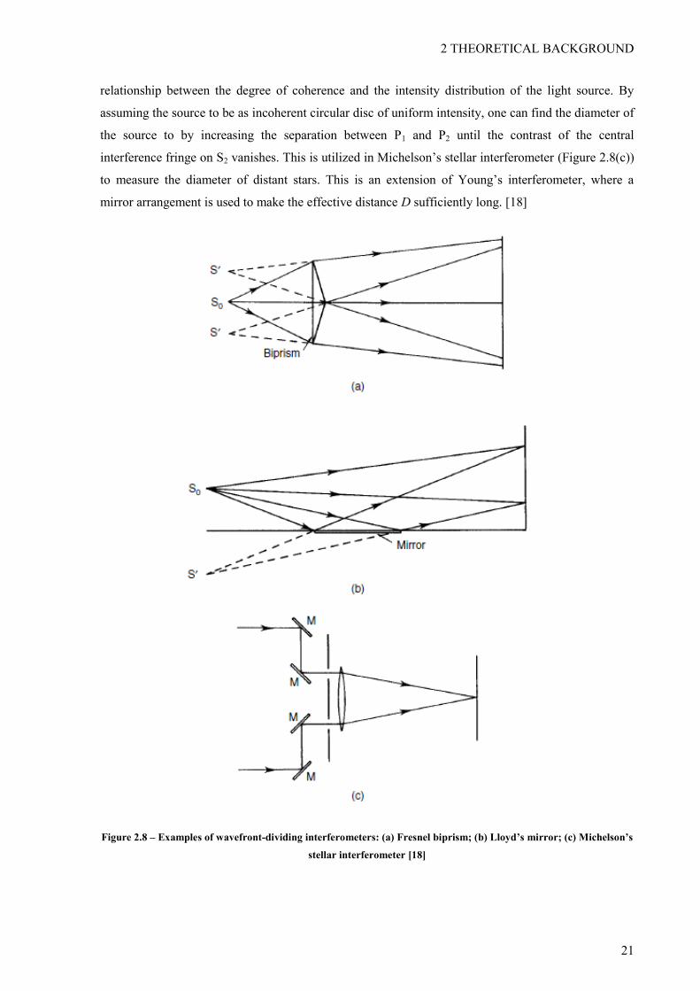
2 THEORETICAL BACKGROUND
21
relationship between the degree of coherence and the intensity distribution of the light source. By
assuming the source to be as incoherent circular disc of uniform intensity, one can find the diameter of
the source to by increasing the separation between P1 and P2 until the contrast of the central
interference fringe on S2 vanishes. This is utilized in Michelson’s stellar interferometer (Figure 2.8(c))
to measure the diameter of distant stars. This is an extension of Young’s interferometer, where a
mirror arrangement is used to make the effective distance D sufficiently long. [18]
Figure 2.8 – Examples of wavefront-dividing interferometers: (a) Fresnel biprism; (b) Lloyd’s mirror; (c) Michelson’s
stellar interferometer [18]

2 THEORETICAL BACKGROUND
22
Amplitude Division The most well-known amplitude-dividing interferometer is the Michelson interferometer, which can
be seen in Figure 2.9. Here the amplitude of the incident light field is divided by the beamsplitter BS
which is partly reflecting. The reflected and the transmitted partial waves propagate to the mirrors M1
and M2 respectively, from where they are reflected back and recombine to form the interference
distribution on the detector D.
Figure 2.9 – Michelson’s interferometer [18]
The path-length difference between the two partial waves can be varied by moving one of the mirrors.
A displacement x of M2 gives a path length difference 2x and a phase equal to ( ) . This
results in a total intensity given by
xIxI
4cos12)(
(2.20)
As M2 moves, its displacement is measured by counting the number of light maxima registered by the
detector. By counting the numbers of maxima per unit time, one can find the speed of the object.[18]
2 THEORETICAL BACKGROUND
23
Figure 2.10 – Further examples of amplitude-dividing interferometers: (a) Twyman-Green interferometer; (b) Mach-
Zehnder interferometer [18]
2.2.5 Coherence
Coherence can be broadly described as the property that enables two electromagnetic fields to
interfere. In order to fully grasp the concept, and although the properties of spatial and temporal
coherence are not tantamount to the description of coherent light, they are helpful for an intuitive
understanding of the nature of partially coherent light and will, as such, be briefly described in what
follows.

2 THEORETICAL BACKGROUND
24
In as much as temporal coherence can be described as a measure of the degree of the spectral purity of
a wave, i.e., how monochromatic the radiation is, spatial coherence is a measure of the spatial extent
of the source, an ideal source being confined to a point in space.
Temporal coherence is intimately related to the frequency bandwidth of a truncated wave train. It
determines how far two points along the direction of propagation of a wave can be, and still possess a
definite phase relationship. For that reason, temporal coherence is also called longitudinal coherence.
The Michelson interferometer, which senses longitudinal path differences between the interfering
waves, is ideally suited for investigating temporal coherence of light fields.
Spatial coherence of light fields depends on the physical size of the light source. Light coming from a
point source, which may be taken as a source with dimensions not exceeding the mean wavelength of
the emitted light, possesses a high degree of spatial coherence, irrespective of the frequency bandwidth
of the source.
Commonly observed speckles with laser light reflect a high degree of spatial coherence of laser light,
despite the laser not being a point source. Light from a conventional extended source, on the other
hand, has considerably reduced spatial coherence because different points on an extended source
radiate independently and therefore are mutually incoherent. Light emanating from an extended source
cannot be characterized by a definite state of spatial coherence. Also, the spatial coherence of light
from an extended source changes as light propagates.
Spatial coherence of light determines how far two points can lie in a plane transverse to the direction
of propagation of light and still be correlated in phase. Spatial coherence of light can be investigated
by interferometers of the type used by Young in is famous two-slit interference experiment. [17]
Detection of light is an averaging process in space and time. In developing equation (2.12) no
averaging was made because it was assumed the phase difference to be constant in time. Ideally, a
light wave with a single frequency must have an infinite length. Therefore, sources emitting light of a
single frequency do not exist.
One way of illustrating the light emitted by real sources is to picture it as sinusoidal wave trains of
finite length with randomly distributed phase differences between the individual trains.
In Figure 2.11 two successive wave trains of the partial waves are sketched. The two wave trains have
equal amplitude and length Lc, with an abrupt, arbitrary phase difference. Figure 2.11 (a) shows the
situation when the two partial waves have travelled equal path lengths. Although the phase of the
original wave fluctuates randomly, the phase difference between the partial waves 1 and 2 remains
constant in time. The resulting intensity is therefore given by equation (2.12). Figure 2.11 (c) shows
the situation when partial wave 2 has travelled a path length Lc longer than partial wave 1. The head of
the wave trains in partial wave 2 then coincide with the tail of the corresponding wave trains in partial
wave 1. The resulting instantaneous intensity is still given by equation (2.12), but now the phase

2 THEORETICAL BACKGROUND
25
difference fluctuates randomly as the successive wave trains pass by. As a result, varies
randomly between +1 and -1. When averaged over many wave trains, therefore becomes zero
and the resulting, observable intensity will be
21 III (2.21)
Figure 2.11 – Wave trains of the partial waves [18]
Figure 2.11 (b) shows an intermediate case where partial wave 2 has travelled a path length l longer
than partial wave 1, where 0 < l < Lc. Averaged over many wave trains, the phase difference now
varies randomly in a time period proportional to and remains constant in a time period
proportional to where . The result is that is still possible to observe an interference
pattern according to equation (2.12), but with a reduced contrast. To account for this loss of contrast,
equation (2.12) can be written as
cos2 2121 IIIII (2.22)
Where | ( )| means the absolute value of ( ).
The definition of contrast or visibility is now introduced,
minmax
minmax
II
IIV
(2.23)
Where Imax and Imin are two neighboring maxima and minima of the interference pattern described by
equation (2.22). Since varies between +1 and – 1:

2 THEORETICAL BACKGROUND
26
2121max 2 IIIII (2.24)
2121min 2 IIIII (2.25)
Which, inserting on equation (2.23) gives:
21
212
II
IIV
(2.26)
For two waves of equal intensity, , equation (2.26) becomes,
V (2.27)
which shows that in this case | ( )| is exactly equal to the visibility. ( ) is termed the complex
degree of coherence and is a measure of the ability of the two wave fields to interfere. [18]
2.2.6 Two-beam Interferometers
A number of two-wave interferometers exist with countless applications in optics, metrology, plasma
diagnostics, and other related fields. Most of these interferometers are variants of the historic
Michelson interferometer. This will be followed by a brief discussion on other commonly used
interferometers like Mach-Zehnder interferometer and VISAR. All of these interferometers are
amplitude-dividing interferometers.
Michelson interferometer In the Michelson interferometer a beam splitter (a semitransparent mirror) is used to divide the light
into two beams as shown in Figure 2.12.
2 THEORETICAL BACKGROUND
27
Figure 2.12 – Michelson Interferometer [16]
The two beams are directed along orthogonal paths, usually called the arms of the interferometer,
where they strike two mirrors, M1 and M2, and then return to the beam splitter where they interfere.
Looking at the beam splitter from the detector is possible to see an image of mirror M2 near mirror M1.
The image M2’ and the mirror M1 form a dielectric layer of thickness d. The interferometer is assumed
to be in the air so that the dielectric layer has an index of refraction n2=1. Also, light reflected from
M1 and M2 experiences the same phase change upon reflection, thus, no additional phase shift needs
to be added to Δ in calculating the phase difference between the two waves. The total phase difference
for a bright band is
0
cos222
td
m
(2.28)
The source shown in Figure 2.12 is nearly a point source, generating spherical waves that produce
fringes of constant inclination. The fringes are circularly symmetric if d is a constant across the
aperture. The maximum value of m, the order of the fringe, occurs at the center of the set of fringe
rings where θt =0
0
max
2
dm
(2.29)
The order of the fringes is shown by equation (2.29) to be equal to the difference in lengths of the two
interferometer arms expressed in the number of wavelengths of light contained in d.
As d increases, a bright band will move out from the center of the aperture and a new bright band of
higher order will take its place at the center. If the detector is placed at the position of the center fringe
and monitored the intensity as we moved one of the mirrors, and thereby changed d, we should see

2 THEORETICAL BACKGROUND
28
c
dIIIII
2cos2 2121
(2.30)
Where
0
2
c
(2.31)
If the beam splitter is a 50:50 splitter, then the intensity of the light in the two arms will be the same:
c
dII
2cos10
(2.32)
If we use the physical arrangement shown in Figure 2.12, the light in the M1 arm of the interferometer
travels an extra distance 2d to reach the detector. This means that two waves are added together that
originated at different times; the difference in time between the origination of two waves is:
c
d2
(2.33)
Which is called the retardation time (the wave in arm M1 has been delayed or retarded). Using the
equation (2.33),
cos10 II (2.34)
The signal is made up of a constant term plus an oscillatory term. The oscillatory term will provide
information about the coherence properties of the light. [16]
Mach-Zehnder Interferometer The Mach-Zehnder interferometer is another amplitude splitting device. As shown in Figure 2.13, is
consists of two beam splitters and two totally reflecting mirrors. The two waves within the apparatus
travel along separate paths. A difference between the optical paths can be introduced by a slight tilt of
one of the beam splitters. Since the two paths are separated, the interferometer is relatively difficult to
align. For the same reason, however, the interferometer finds myriad applications. It has even been
used, in a somewhat altered yet conceptually similar from, to obtain electron interference fringes.
2 THEORETICAL BACKGROUND
29
Figure 2.13 – Mach-Zehnder interferometer [14]
An object interposed in one beam will alter the optical path length difference, thereby changing the
fringe pattern. A common application of the device is to observe the density variations in gas-flow
patterns within research chambers. One beam passes through the optically flat windows of the test
chamber, while the other beam transverses appropriate compensator plates. The beam within the
chamber will propagate through regions having a spatially varying index of refraction. [14]
VISAR system The VISAR (Velocity Interferometer System for Any Reflector) is a robust tool widely used to
measure surface velocities optically. This technique was developed by Barker and Hollenbach based in
two previous techniques, the Wide Angle Michelson Interferometer (WAMI) and the Lockheed Laser
Velocimeter.
VISAR is a homodyne technique, this means that, the Doppler-shifted light is divided in two optical
ways of differing length and recombined at the photo detector. In short, VISAR does not truly measure
the Doppler shift, it measures the difference in the Doppler shift between two relatively Doppler
shifted reflected light beams. Since the introduction of VISAR, it has gone through several evolutions
like the multipoint VISAR, fixed cavity VISAR, among others.
As referred before, VISAR consists in an unequal leg Michelson interferometer where monochromatic
light reflected from a target is divided and transverses two legs. One of those legs, despite the distance
along both tracks appears to be the same, has a longer delay time, so that when the beams recombined
at the beam splitter mirror, is produced the interference that contains the Doppler-shift changes of the
moving target. [19]
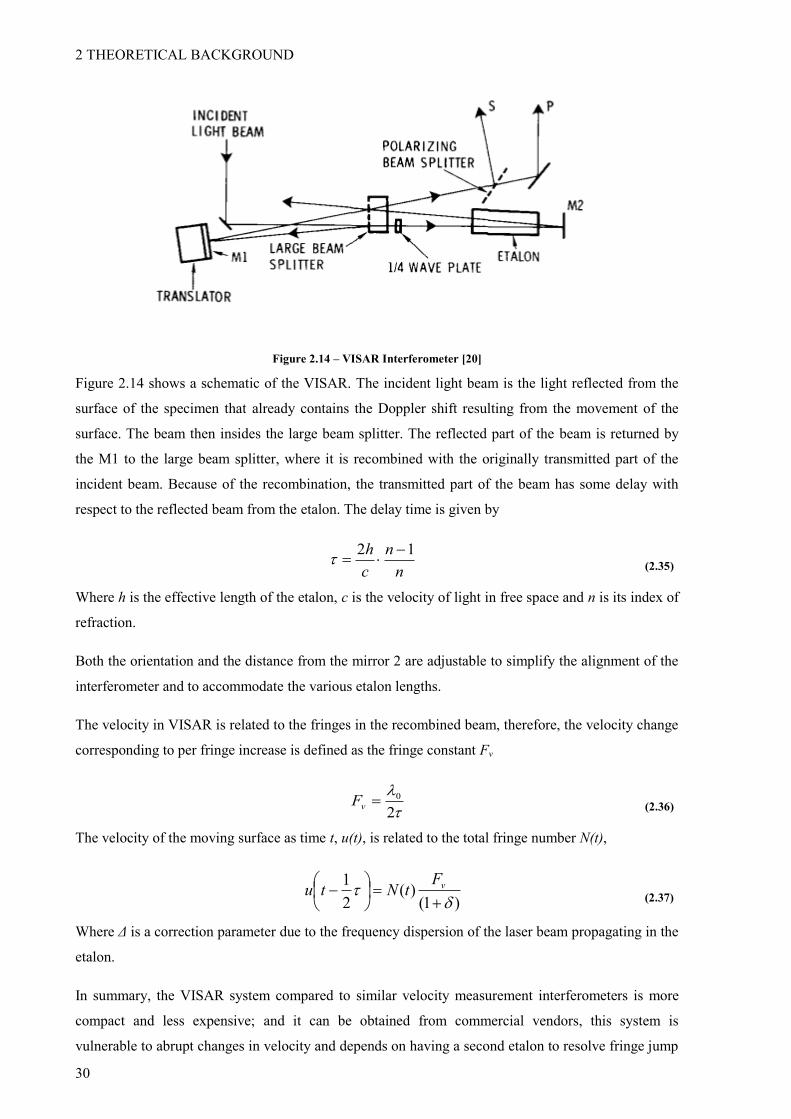
2 THEORETICAL BACKGROUND
30
Figure 2.14 – VISAR Interferometer [20]
Figure 2.14 shows a schematic of the VISAR. The incident light beam is the light reflected from the
surface of the specimen that already contains the Doppler shift resulting from the movement of the
surface. The beam then insides the large beam splitter. The reflected part of the beam is returned by
the M1 to the large beam splitter, where it is recombined with the originally transmitted part of the
incident beam. Because of the recombination, the transmitted part of the beam has some delay with
respect to the reflected beam from the etalon. The delay time is given by
n
n
c
h 12
(2.35)
Where h is the effective length of the etalon, c is the velocity of light in free space and n is its index of
refraction.
Both the orientation and the distance from the mirror 2 are adjustable to simplify the alignment of the
interferometer and to accommodate the various etalon lengths.
The velocity in VISAR is related to the fringes in the recombined beam, therefore, the velocity change
corresponding to per fringe increase is defined as the fringe constant Fv
2
0vF (2.36)
The velocity of the moving surface as time t, u(t), is related to the total fringe number N(t),
)1()(
2
1
vF
tNtu (2.37)
Where Δ is a correction parameter due to the frequency dispersion of the laser beam propagating in the
etalon.
In summary, the VISAR system compared to similar velocity measurement interferometers is more
compact and less expensive; and it can be obtained from commercial vendors, this system is
vulnerable to abrupt changes in velocity and depends on having a second etalon to resolve fringe jump

2 THEORETICAL BACKGROUND
31
ambiguities. For data analysis, VISAR uses absolute intensities to obtain the velocity information.
This system, like other laser interferometers, requires very precise alignment and adjustment of the
optical elements. It can measure the material velocity with 1% accuracy and a resolution better than 1
ns. By changing the etalon, it is possible to increase the range of measurable velocities [19-28]
2.2.7 Multiple-beam Interference
A number of situations in which two coherent beams are combined under diverse conditions to
produce interference patterns have been scrutinized. There are, however, circumstances under which a
much larger number of mutually coherent waves are made to interfere. In fact, whenever the
amplitude-reflection coefficients, the r’s, for the parallel plate illustrated in Figure 2.15 are not small,
the higher-order reflected waves
,… become quite significant. A glass plate, slightly silvered
on both sides so that the r’s approach unity, will generate a large number of multiply internally
reflected rays.
Figure 2.15 – Multiple-beam interference from a parallel film [17]
To begin the analysis as simple as possible, let the film be non-absorbing and n1 = n2. The amplitude-
transmission coefficients are represented by t, the fraction of the amplitude of a wave transmitted on
entering into the film, and t’, the fraction transmitted when a wave leaves the film.
As shown in Figure 2.15 – Multiple-beam interference from a parallel film [17], the scalar amplitudes
of the reflected waves
, …, are respectively
, …, where E0 is the
amplitude of the initial incoming wave and r = – r’. The minus sign indicates a phase shift. Similarly,
the transmitted waves
, … will have amplitudes
, …. [14]
Each transmitted wave will have a constant phase difference, relative to its neighbor,

2 THEORETICAL BACKGROUND
32
0
2 cos4
tdn
(2.38)
Where .
The intensity of the transmitted light is,
2
sin41 2222
2
rr
EI
(2.39)
When
22
2
max
1 r
EI
(2.40)
When
22
2
min
1 r
EI
(2.41)
The fringe visibility is a useful characterization of interference; the larger the value of this parameter,
the easier it is to observe the fringe pattern. The maximum value of fringe visibility is 1 and occurs
when ; the minimum value is zero and occurs when . Using equation (2.40) and
(2.41) in (2.10), it is obtained the fringe visibility in terms of the reflectivity of the film surface
As the reflectivity approaches 1, the fringe visibility approaches its maximum value of 1.
The intensity transmitted through the dielectric layer in terms of is,
2sin
1
41 2
22
2
max
r
r
II
(2.42)
The factor
F
r
r
22
2
1
4
(2.43)
Is called the contrast F and its use allows the relative transmission of the dielectric layer to be
expressed in a format called the Airy function.

2 THEORETICAL BACKGROUND
33
2sin1
1
2max
FI
I
(2.44)
Plotting the Airy function for different values of the reflectivity r2 is possible to obtain the Figure 2.16
which displays a periodic maximum in the transmission of the dielectric layer as δ is varied. The peak
in transmission occurs when d is equal to a multiple of , where λ is the illuminating wavelength.
Thus, the maximum transmission of the film thickness will support standing waves in the layer, that is,
the transmission maxima occurs for eigenvalues of the layer. [16]
Figure 2.16 – Plot of the fraction of transmitted light as a function of the optical path length [16]
The peak transmission in Figure 2.16 narrows as the reflectivity r2 increases. The value of δ over
which I goes from Imax to Imax/2 is a measure of the fringe sharpness and can be obtained by noting
when δ=0. When ,
( )
The fringe sharpness is given by
Fr
r 1sin2
2
1sin2 1
21
2/1 (2.45)
The sharpness of the fringes increases and δ1/2 decreases with increasing reflectivity.

2 THEORETICAL BACKGROUND
34
Fabry-Perot interferometer Fabry Perot interferometer, Figure 2.17, consists of two plane, parallel, highly reflecting surfaces
separated by a distance d. This is the simplest configuration. and other forms are also widely used. In
practice, two semi-silvered or aluminized glass optical flats form the reflecting boundary surfaces. The
enclosed air gap generally ranges from several millimetres to several centimeters when the apparatus
is used interferometrically, and often to considerably greater lengths when it serves as a laser resonant
cavity.
Figure 2.17 – Experimental arrangement of a Fabry-Perot interferometer [16]
The waves in the plates, after multiple reflections, are collected by the lens and imaged on an
observation screen. Only one propagation vector, incident at an angle θ, is followed through the
system in Figure 2.17. Other incident propagation vectors will result in a bright band if . The
incident angle of propagation vectors forming the bright bands must satisfy the equation
cos2ndm (2.46)
The observed fringes, such as those in Figure 2.18 – Output fringes from a Fabry-Perot interferometer
[16]are circularly symmetric if the illumination is symmetric about the symmetry axis of the optical
system.

2 THEORETICAL BACKGROUND
35
Figure 2.18 – Output fringes from a Fabry-Perot interferometer [16]
The accuracy with which an interferometer can measure the wavelength of its illumination is called
chromatic resolving power, R, and is defined as , where λ is the mean wavelength of the
illumination and Δλ is the wavelength difference that can be resolved. The criterion for resolution
assumes that two wavelengths λ1 and λ2 of equal intensity are present. The criterion for resolution of
the two wavelengths states that the two wavelengths are just resolved if the half-maximum intensity of
a fringe produced by λ1 falls on the half-maximum intensity of a fringe produced by λ2. When this
occurs, the transmitted intensity is a constant as d is varied from the resonant condition of λ1 to the
resonant condition of λ2. The phase shift in going from the intensity maximum for λ1 to the intensity
maximum for λ2 is then Δδ=2δ1/2. The fringes are assumed to be narrow so that this is a small value
with the approximation
And
(
)
A bright band will occur whenever
mdn t cos2 2 (2.47)
The relationship between Δθ and Δλ is
dn
mtt
22sin
(2.48)
The resolving power is thus

2 THEORETICAL BACKGROUND
36
Fm
r
rm
21 2
R
(2.49)
From equation (2.47) is possible to see that the order number m has a maximum value whenever
, that is, m is a maximum at the center of the Fabry-Perot fringe pattern and this maximum
is given by
0
2max
2
dnm
(2.50)

2 THEORETICAL BACKGROUND
37
2.3 Heterodyne technique
Heterodyne interferometry is on of the most flexible and accurate interferometric surface profile or
displacement measurement techniques available today, there being current commercial systems
available for the measurement of nm ranges with sub-Angstrom accuracy to 60 m ranges or 100 mm
ranges to 1 part in 108 accuracy. An elegant exposé of a full-field, real time measurement system to
λ/100 accuracy tested on 5 cm mirrors was made by Massie in 1979. Remarkable 0.1 mm resolution
for 100 m ranges have also been reported and a Super Heterodyne interferometer using two laser
wavelengths and two heterodyning frequencies simultaneously was described by Tiziani with a
striking 50 µm resolution for 100 m ranges.
Figure 2.19 – Phase locked laser diode interferometer [29]
Heterodyning, or better still Homodyning since two light beams of different frequencies are derived by
a frequency offset process from a single, parent laser beam source in this case, is the use of frequency
beats from these two very similar frequencies to determine the phase difference introduced by an
object onto one of them. [29]
Therefore, if a frequency difference is introduced between the two beams in an interferometer, the
electric fields due to them at any point P can be represented by the relations
)2cos()( 1111 tatE (2.51)
And
)2cos()( 2222 tatE (2.52)

2 THEORETICAL BACKGROUND
38
Where a1 and a2 are the amplitudes, ν1 and ν2 the frequencies, and 1 and 2 the phases, relative to
the origin, of the two waves at the point P. The resultant intensity at P is then
212121212121
22
2
211
2
1
2
2
2
1
2
21
)(2cos)(2cos
4cos4cos21)2/()2/(
)()()(
taataa
tataaa
tEtEtI
(2.53)
The output from a photo detector, which cannot respond to the components at frequencies of 2ν1, 2ν2,
and (ν1+ ν2) is, therefore,
)()(2cos)(2)( 2121
21
2121 tIIIItI (2.54)
Where ( ) and (
). The phase of the oscillatory component, at the difference
frequency (ν1 – ν2), gives the phase difference between the interfering waves at P, directly. [15]
2.4 LDV
Laser Doppler Velocimetry, as the name indicates is a method for measuring the velocity of, for
example, moving objects or particles. [18]
The laser Doppler technique uses monochromatic laser light as a light source. The interference of two
beams crossing in the measurement volume or the interference of two scattering waves on the detector
creates a fringe pattern. The velocity information for moving scattering centers is contained in the
scattered field due to the Doppler Effect. The laser Doppler technique is an indirect measuring
technique, since it measures the velocity of inhomogeneities in the flow, typically tracer particles. This
represents the flow velocity only if no appreciable slip velocity is present. Otherwise the slip velocity
must also be determined.
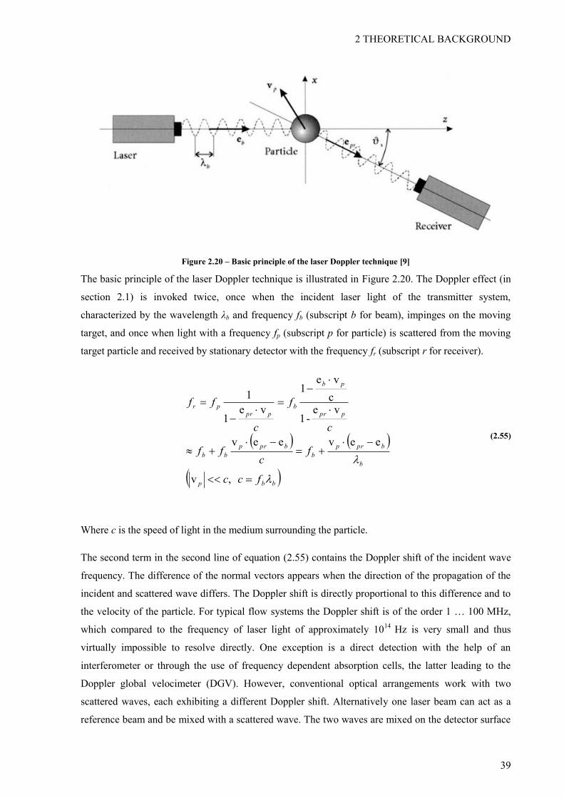
2 THEORETICAL BACKGROUND
39
Figure 2.20 – Basic principle of the laser Doppler technique [9]
The basic principle of the laser Doppler technique is illustrated in Figure 2.20. The Doppler effect (in
section 2.1) is invoked twice, once when the incident laser light of the transmitter system,
characterized by the wavelength λb and frequency fb (subscript b for beam), impinges on the moving
target, and once when light with a frequency fp (subscript p for particle) is scattered from the moving
target particle and received by stationary detector with the frequency fr (subscript r for receiver).
bbp
b
bprp
b
bprp
bb
ppr
pb
b
ppr
pr
fcc
fc
ff
c
f
c
ff
,v
eeveev
ve-1
c
ve1
ve1
1
(2.55)
Where c is the speed of light in the medium surrounding the particle.
The second term in the second line of equation (2.55) contains the Doppler shift of the incident wave
frequency. The difference of the normal vectors appears when the direction of the propagation of the
incident and scattered wave differs. The Doppler shift is directly proportional to this difference and to
the velocity of the particle. For typical flow systems the Doppler shift is of the order 1 … 100 MHz,
which compared to the frequency of laser light of approximately 1014
Hz is very small and thus
virtually impossible to resolve directly. One exception is a direct detection with the help of an
interferometer or through the use of frequency dependent absorption cells, the latter leading to the
Doppler global velocimeter (DGV). However, conventional optical arrangements work with two
scattered waves, each exhibiting a different Doppler shift. Alternatively one laser beam can act as a
reference beam and be mixed with a scattered wave. The two waves are mixed on the detector surface

2 THEORETICAL BACKGROUND
40
in a process known as optical heterodyning, yielding the beat frequency, which typically lies in a much
more manageable frequency range for signal processing.
There are several alternatives to practically realize such systems using one incident beam, such as, a
dual-scattered wave system, Figure 2.21 (a) and one-reference beam, Figure 2.21 (b).
Figure 2.21 – System using one incident beam; (a) Dual-beam scattering configuration; (b) Reference-beam
configuration [9]
In both cases the difference (beat) frequency fd is obtained through the optical mixing of waves with
frequencies f1 and f2 on the detector. For the one-beam configurations these frequencies are given as
Dual-scattered-wave configuration (Figure 2.21 (a)):
b
bpp
b
b
bpp
b ffff
eev,
eev 2
2
1
1
(2.56)
b
ppp
D fff
12
12
eev (2.57)
Reference-beam configuration (Figure 2.21 (b)):
b
b
bpp
b ffff
2
1
1 ,eev
(2.58)
b
pbp
D fff
1
12
eev (2.59)
The measurement volume is defined in both cases using an aperture on the detector, thus a virtual
measurement volume is realized.

2 THEORETICAL BACKGROUND
41
The more widely used optical configuration is based on two incident waves, as illustrated in Figure
2.22.
In the dual-beam configuration (Figure 2.22 (a)), a real measurement volume is formed at the
intersection of the two incident waves and the scattered waves are detected with a single
detector:
b
prp
b
b
prp
b ffff
2
2
1
1
eev,
eev
(2.60)
b
p
D fff
21
12
eev (2.61)
Figure 2.22 – Optical configuration for two incident waves; (a) dual-beam configuration; (b) reference-beam
configuration [9]
In the reference-beam configuration (Figure 2.22 (b)), the detector is positioned directly in the
path of one of the beams ( ). Typically the incident reference beam is much lower in
intensity than the incident scattering beam. This configuration is seldom used; however, it
does show some advantages for measurements in highly absorbing media.
1
2
21 ee,eev
,
pr
b
prp
bb ffff
(2.62)
b
p
D fff
21
12
eev (2.63)
The difference frequency is independent of the receiver position for the dual-beam configurations in
Figure 2.22.
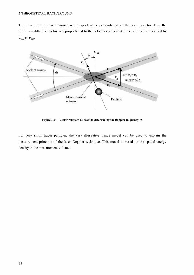
2 THEORETICAL BACKGROUND
42
The flow direction α is measured with respect to the perpendicular of the beam bisector. Thus the
frequency difference is linearly proportional to the velocity component in the x direction, denoted by
or .
Figure 2.23 – Vector relations relevant to determining the Doppler frequency [9]
For very small tracer particles, the very illustrative fringe model can be used to explain the
measurement principle of the laser Doppler technique. This model is based on the spatial energy
density in the measurement volume.

2 THEORETICAL BACKGROUND
43
Figure 2.24 – Generation of the interference structure of two homogenous waves. (a) (b) Electric field strength of
incident waves; (c) Superposition of electric fields; (d) Intensity [9]
The spatial dependence of the intensity in the intersection volume can be interpreted as an interference
field with fringes parallel to the y-z plane (Figure 2.24). The fringe spacing is given by:
2sin2
bx
(2.64)

2 THEORETICAL BACKGROUND
44
This interference or fringe model of the laser Doppler technique is strictly only valid for very small
particles fulfilling the condition , since only then can the amplitude and phase, or intensity of
the field be considered constant over the particle diameter.
For particles larger than the wavelength of light this model fails. Both the amplitude and phase of the
incident waves vary across the diameter of the particle.
Only certain areas of the particle surface are involved in defining signal properties. The position and
size of the receiving aperture define the position and size of these interaction areas. The area of the
first interaction with the field is known as the “incident point” and the source area of the scattered
wave is called “glare point”, Figure 2.25. The size of the incident areas/“points” and glare
areas/“points” is proportional to the size of the detection aperture.
The scattered waves detected by the receiver each have an amplitude, which depends on the position
of their glare points.
Figure 2.25 – Signal origin for large particles [9]
A conventional laser Doppler optical arrangement is summarized in Figure 2.26. The laser beam is
split into two beams of equal intensity and polarization using a beam splitter and brought to
intersection with a lens. A collimator is used for adjusting the beam properties in the measurement
volume and the Bragg cell provides a frequency shift used for directional sensitivity. The Doppler
frequency is determined using a signal processor and the data analysis for computing flow properties
is performed in a computer.

2 THEORETICAL BACKGROUND
45
Figure 2.26 – Dual-beam laser Doppler Velocimetry [9]
The laser Doppler technique samples the flow velocity at discrete times corresponding to the passage
of a particle through the intersection volume. [9]
2.5 PDV
Photon Doppler Velocimetry is a heterodyne velocimeter technique based on the the LDV, where the
frequency of the Doppler-shifted light provides a direct measure of the instantaneous velocity of a
moving target illuminated by a laser. With the developments in telecommunications technologies, the
Lawrence Livermore National Laboratory (LLNL) developed a novel fiber-optic approach LDV as a
diagnostic for high explosive tests. This technique is able to measure surface velocities ranging from
centimeters per second to kilometers per second.
The technique uses multi-mode fiber optics operating at 1550 nm, along with many high-bandwidth
electrical components. The choice of a wavelength which is popular in telecommunications, serves
both the necessity of working with a rather large wavelength and the low cost of the required
components. As a Michelson interferometer counts fringes for measuring distances with x = n/2,
the measured velocities obey the relation V = F/2. As such, an object moving at 1 km/s will exhibit a
frequency of approximately 1.29 GHz, already rather high. Smaller wavelengths would require even
higher frequency detection bandwidths, and necessarily more expensive detection equipment. Figure
2.27 shows the basics of the photonic Doppler Velocimetry system.
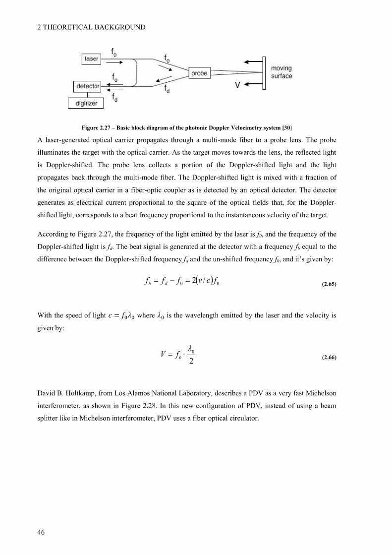
2 THEORETICAL BACKGROUND
46
Figure 2.27 – Basic block diagram of the photonic Doppler Velocimetry system [30]
A laser-generated optical carrier propagates through a multi-mode fiber to a probe lens. The probe
illuminates the target with the optical carrier. As the target moves towards the lens, the reflected light
is Doppler-shifted. The probe lens collects a portion of the Doppler-shifted light and the light
propagates back through the multi-mode fiber. The Doppler-shifted light is mixed with a fraction of
the original optical carrier in a fiber-optic coupler as is detected by an optical detector. The detector
generates as electrical current proportional to the square of the optical fields that, for the Doppler-
shifted light, corresponds to a beat frequency proportional to the instantaneous velocity of the target.
According to Figure 2.27, the frequency of the light emitted by the laser is f0, and the frequency of the
Doppler-shifted light is fd. The beat signal is generated at the detector with a frequency fb equal to the
difference between the Doppler-shifted frequency fd and the un-shifted frequency f0, and it’s given by:
00 /2 fcvfff db (2.65)
With the speed of light where is the wavelength emitted by the laser and the velocity is
given by:
2
0 bfV (2.66)
David B. Holtkamp, from Los Alamos National Laboratory, describes a PDV as a very fast Michelson
interferometer, as shown in Figure 2.28. In this new configuration of PDV, instead of using a beam
splitter like in Michelson interferometer, PDV uses a fiber optical circulator.
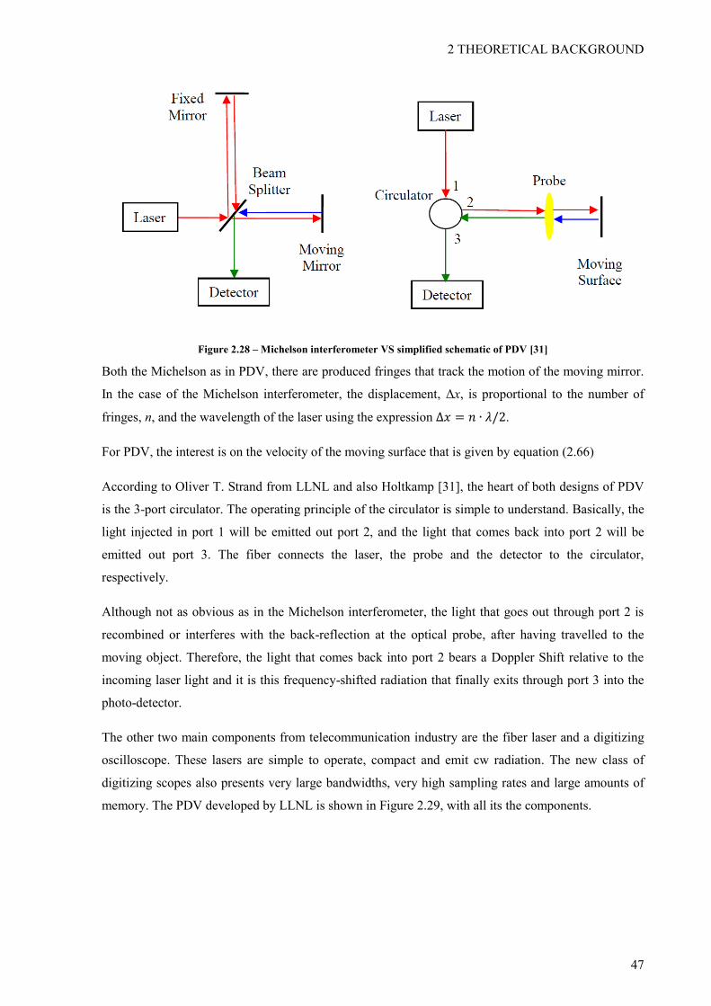
2 THEORETICAL BACKGROUND
47
Figure 2.28 – Michelson interferometer VS simplified schematic of PDV [31]
Both the Michelson as in PDV, there are produced fringes that track the motion of the moving mirror.
In the case of the Michelson interferometer, the displacement, Δx, is proportional to the number of
fringes, n, and the wavelength of the laser using the expression .
For PDV, the interest is on the velocity of the moving surface that is given by equation (2.66)
According to Oliver T. Strand from LLNL and also Holtkamp [31], the heart of both designs of PDV
is the 3-port circulator. The operating principle of the circulator is simple to understand. Basically, the
light injected in port 1 will be emitted out port 2, and the light that comes back into port 2 will be
emitted out port 3. The fiber connects the laser, the probe and the detector to the circulator,
respectively.
Although not as obvious as in the Michelson interferometer, the light that goes out through port 2 is
recombined or interferes with the back-reflection at the optical probe, after having travelled to the
moving object. Therefore, the light that comes back into port 2 bears a Doppler Shift relative to the
incoming laser light and it is this frequency-shifted radiation that finally exits through port 3 into the
photo-detector.
The other two main components from telecommunication industry are the fiber laser and a digitizing
oscilloscope. These lasers are simple to operate, compact and emit cw radiation. The new class of
digitizing scopes also presents very large bandwidths, very high sampling rates and large amounts of
memory. The PDV developed by LLNL is shown in Figure 2.29, with all its the components.

2 THEORETICAL BACKGROUND
48
Figure 2.29 – Components used in PDV [24]
This equipment is durable, relatively inexpensive and easy to use, and data analysis can be performed
rapidly. The maximum velocity is limited by the bandwidth of the electronics and the sampling rate of
the digitizers.
The heterodyne system responds to the absolute value of the beat frequency, and it can’t make the
difference between a surface moving toward or away from the probe, what can make this method less
useful in applications where the absolute position of the surface must be followed.
There are advantages and disadvantages on using this technique, the advantages significantly out-
weighting the disadvantages. One of the main advantages is the fact that the beat frequency is lower
for a given velocity than it would be using visible light lasers, and one chief disadvantage of operating
this king of lasers (1550 nm) is the fact that the laser radiation cannot be seen with the unaided eye
therefore, some practical issues of performing probe alignments with respect to the target surface are
difficult to circumvent. [5, 6, 24, 30-32]
2.6 Fourier transform
A very large class of important computational problems falls under the general rubric Fourier
transform methods or spectral methods. For some of the problems, the Fourier transform is just an
efficient computational tool for accomplishing certain common manipulations of data. In other cases,
there are problems for which the Fourier transform is itself of intrinsic interest.
A physical process can be described either in the time domain, by the values of some quantity h as a
function of time t, e.g., h(t), or else in the frequency domain, where the process is specified by giving

2 THEORETICAL BACKGROUND
49
its amplitude H as a function of frequency f, that is, H(f), with . For many purposes it is
useful to think of h(t) and H(f) as being two different representations of the same function. One goes
back and forth between these two representations by means of the Fourier transform equations,
dfefHth
dtethfH
ift
ift
2
2
)()(
)(
(2.67)
If t is measured in seconds, then f in Eq. (2.67) is measured in cycles per second, or Hertz. However,
the equations work with other units, too. If h is a function of position x (in meters), H will be a
function representing inverse wavelength or spatial frequency, in cycles per meter, and so on.
From Eq. (2.67) it is evident at once that Fourier transformation is a linear operation. The transform of
the sum of two functions is equal to the sum of the transforms. The transform of a constant times a
function is that same constant times the transform of the function.
In the time domain, the function h(t) may happen to have one or more special symmetries. It might be
purely real or purely imaginary or it might be even, ( ) ( ), or odd, ( ) ( ). In the
frequency domain, these symmetries lead to relationships between H(f) and H(-f).
Some other elementary properties of the Fourier transform are shown below, where the “↔” symbol
indicates transform pairs. Some of the most common pairs are:
)()( fHth (2.68)
a
fH
aath
1)( Time scaling
(2.69)
bfHb
th
b
1 Frequency scaling
(2.70)
02
0
iftefHtth
Time shifting
(2.71)
0
2 0 ffHethtif
Frequency shifting (2.72)
With two functions h(t) and g(t), and their corresponding Fourier transforms H(f) and G(f), it is
possible to form combinations of special interest. The convolution of the two functions, denoted ,
is defined by
dthtghg (2.73)

2 THEORETICAL BACKGROUND
50
A special result called the convolution theorem, states that the Fourier transform of the convolution is
just the product of the individual Fourier transforms.
The correlation of two functions, denoted Corr(g, h), is defined by
dhtghg,Corr (2.74)
The correlation is a function of t, which is called the lag. It therefore lies in the time domain, and it
turns out to be one member of the transform pair:
fHfGhg ,Corr (2.75)
This result shows that multiplying the Fourier transform of one function by the complex conjugate of
the Fourier transform of the other gives the Fourier transform of their correlation.
The total power in a signal is the same whether is computed in time or in frequency domain. This
result is known as Parseval’s theorem:
dffHdtthpowertotal
22 2.76
The Fourier Transform therefore is the tool used in spectral analysis. Several examples of its
application to signals acquired in the course of the experimental work can be seen in Chapter 4 on
Data Analysis. [33]
2.7 Split Hopkinson Pressure Bar
Nowadays there are several engineering applications where the impact velocity is important, so, it is
important to proper understand the materials behavior under dynamic deformations.
For a dynamic characterization of materials, there are several methods currently available.[4]
The Split Hopkinson Pressure Bar or Kolsky bar is the most convenient system for characterizing high
strain-rate behavior of materials. This technique was developed by Hopkinson and later by Kolsky,
originally for compression tests, now adapted to tensile tests. [34]
The Hopkinson bar used in the project has been applied to perform high speed tensile tests. As the
scheme in Figure 2.30 shows, this configuration is composed by two bars, an input and output bar, an
impactor that is struck in one end of the input bar and finally the specimen, which is positioned
between the input and the output bars.

2 THEORETICAL BACKGROUND
51
Figure 2.30 – Scheme of a split Hopkinson pressure bar for tensile tests [35]
The impact caused at the far end of the input bar generates a stress-wave that propagates along the bar.
When this wave reaches the specimen its deformation starts and afterwards, the transmitted wave
propagates into the output bar while the reflected wave propagates back into the input bar. These three
waves are measured using strain gages that are placed in the bars on a specific place. Assuming then
that force equilibrium exists between the two sides of the specimen, the stress, strain and strain rate
can be calculated.[35, 36]
2.8 Electromagnetic forming
Electromagnetic forming is one of the High Speed Metal Forming techniques. The process basically
consists of a capacitor bank, a forming coil and a workpiece to be deformed, preferably made of a
material with high electrical conductivity, and it is based on the discharge of a significant quantity of
energy in an extremely short time.
This technique uses pulsed magnetic fields to apply forces to the metal workpiece.
Figure 2.31 – Scheme of Electromagnetic Forming process [7]
The energy required to the deformation of the workpiece is secured by the capacitor bank that is
connected to the process actuator. When the main switch is closed, a high current pulse is discharged
by the capacitor bank into the forming coil. This results in a strong transient magnetic field developed
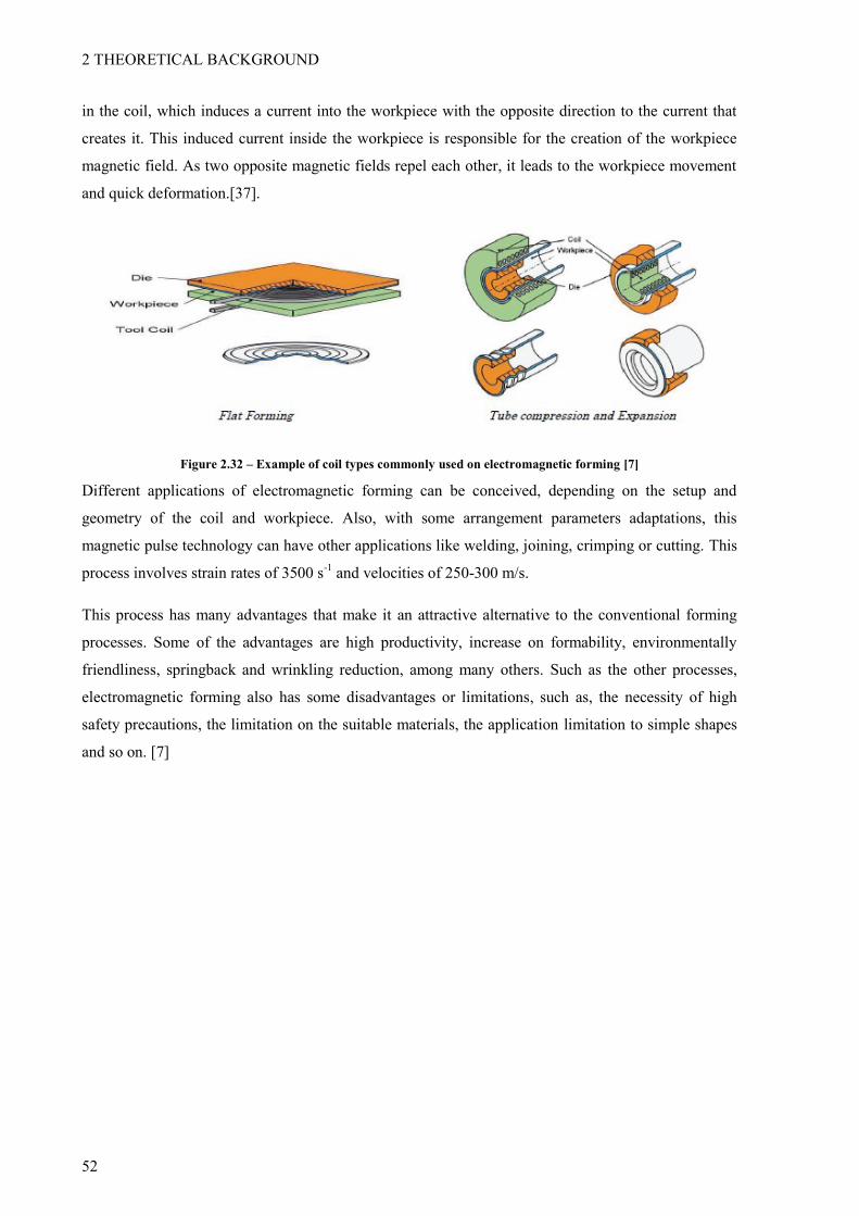
2 THEORETICAL BACKGROUND
52
in the coil, which induces a current into the workpiece with the opposite direction to the current that
creates it. This induced current inside the workpiece is responsible for the creation of the workpiece
magnetic field. As two opposite magnetic fields repel each other, it leads to the workpiece movement
and quick deformation.[37].
Figure 2.32 – Example of coil types commonly used on electromagnetic forming [7]
Different applications of electromagnetic forming can be conceived, depending on the setup and
geometry of the coil and workpiece. Also, with some arrangement parameters adaptations, this
magnetic pulse technology can have other applications like welding, joining, crimping or cutting. This
process involves strain rates of 3500 s-1
and velocities of 250-300 m/s.
This process has many advantages that make it an attractive alternative to the conventional forming
processes. Some of the advantages are high productivity, increase on formability, environmentally
friendliness, springback and wrinkling reduction, among many others. Such as the other processes,
electromagnetic forming also has some disadvantages or limitations, such as, the necessity of high
safety precautions, the limitation on the suitable materials, the application limitation to simple shapes
and so on. [7]

53
3 EXPERIMENTAL WORK
In this section, all steps taken in support of the objective of measuring velocities with a laser will be
described. The initial work served essentially the purpose of getting acquainted with the equipment
available in LOME and grasping the rationale behind the world of Optics and Optical Metrology.
The experimental work therefore began by building a Mach-Zehnder interferometer. This
configuration is important for obtaining interference fringes rapidly and introducing the researcher to
the data analysis of the acquired fringes.
After obtaining the first interference fringes, a Michelson interferometer was assembled, as it basically
works according to the principle of the LDV and after PDV that were envisioned for later deployment.
With a Michelson interferometer it is already possible to measure object velocities, starting with slow
velocities with the Michelson configuration deployed on an active stability control Optical Table and
then gradually increasing the velocities and the confidence on the configured interferometer up until
being able to perform measurements on the Kolsky bar to measure the velocity of its input bar.
The laser used during this experimental work was a Nd:YVO4 laser with a wavelength of
and approximate intensity of 100 mW.
3.1 The Mach-Zehnder Interferometer
The first configuration adopted for the Mach-Zehnder interferometer has the scheme shown in Figure
3.1. This configuration is composed by two mirrors, M1 and M2, and beamsplitters BS1 and BS2.
This first configuration was assembled with the purpose of detecting the fringes created by the
interference of the beams and therefore getting acquainted with the basic principles of interferometry.
Interference is obtained when the beams, originally separated at BS1, are combined at a later stage on
BS2, after travelling different paths.
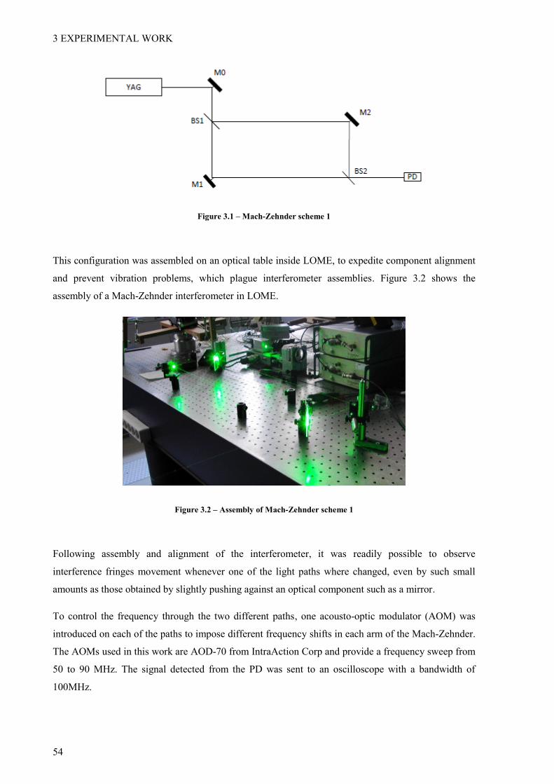
3 EXPERIMENTAL WORK
54
Figure 3.1 – Mach-Zehnder scheme 1
This configuration was assembled on an optical table inside LOME, to expedite component alignment
and prevent vibration problems, which plague interferometer assemblies. Figure 3.2 shows the
assembly of a Mach-Zehnder interferometer in LOME.
Figure 3.2 – Assembly of Mach-Zehnder scheme 1
Following assembly and alignment of the interferometer, it was readily possible to observe
interference fringes movement whenever one of the light paths where changed, even by such small
amounts as those obtained by slightly pushing against an optical component such as a mirror.
To control the frequency through the two different paths, one acousto-optic modulator (AOM) was
introduced on each of the paths to impose different frequency shifts in each arm of the Mach-Zehnder.
The AOMs used in this work are AOD-70 from IntraAction Corp and provide a frequency sweep from
50 to 90 MHz. The signal detected from the PD was sent to an oscilloscope with a bandwidth of
100MHz.
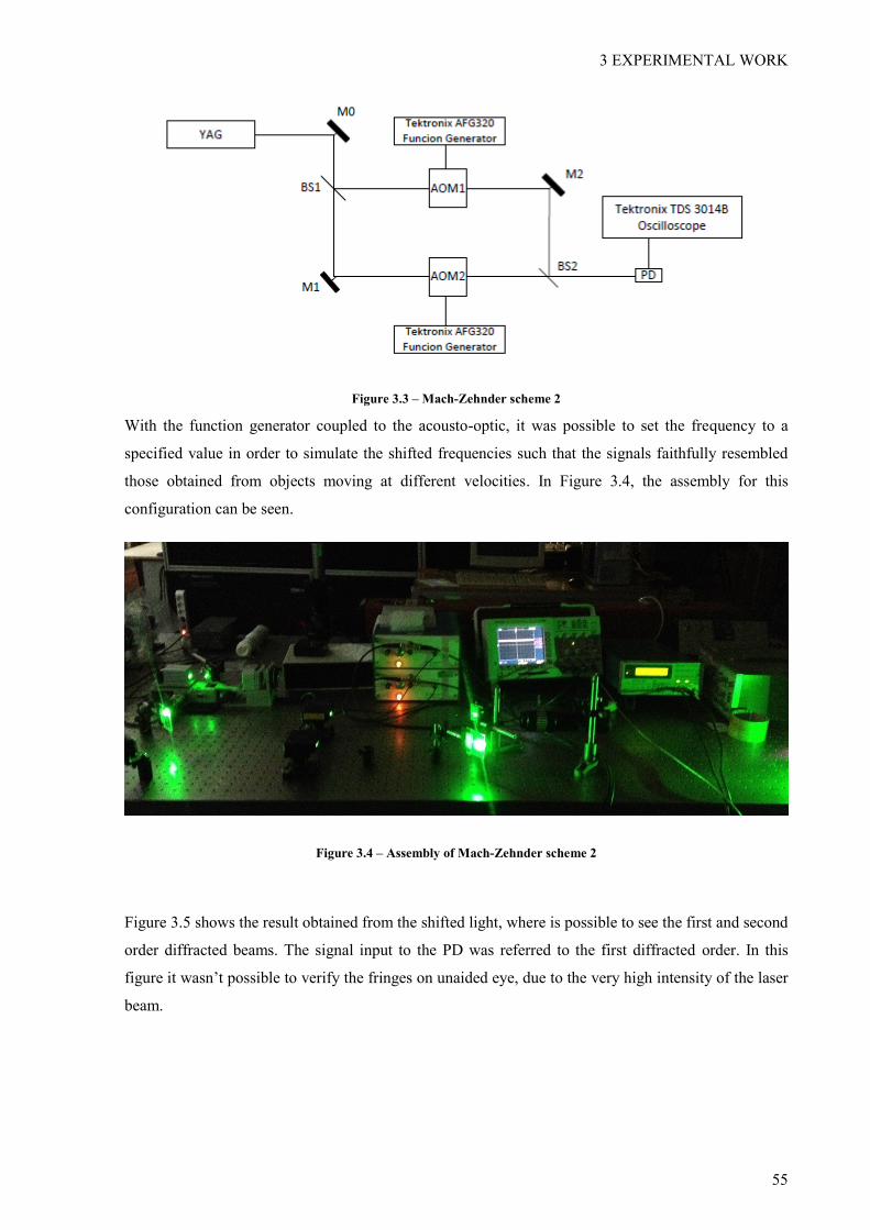
3 EXPERIMENTAL WORK
55
Figure 3.3 – Mach-Zehnder scheme 2
With the function generator coupled to the acousto-optic, it was possible to set the frequency to a
specified value in order to simulate the shifted frequencies such that the signals faithfully resembled
those obtained from objects moving at different velocities. In Figure 3.4, the assembly for this
configuration can be seen.
Figure 3.4 – Assembly of Mach-Zehnder scheme 2
Figure 3.5 shows the result obtained from the shifted light, where is possible to see the first and second
order diffracted beams. The signal input to the PD was referred to the first diffracted order. In this
figure it wasn’t possible to verify the fringes on unaided eye, due to the very high intensity of the laser
beam.

3 EXPERIMENTAL WORK
56
Figure 3.5 – Diffracted beams from Mach-Zehnder scheme 2
The output signal observed in the oscilloscope, that was obtained from the PD, presented too much
noise and very was clearly inconstant. Due to such bad results, an analysis of the components was
started to find out where the noise was originated and
It was concluded that it was due to a bad performance from the acousto-optic modulators that could
not set the frequency input imposed by the function generator. The observed intensities of the beams
coming out of the modulators were also appreciably different from each other.
The oscilloscope available in LOME was also not performant enough for detecting such high
frequencies.
The experimental results from this initial interferometer assembly were therefore compromised by
several equipment related problems and were not as satisfactory as expected, albeit the assemblies
having been done and measurements taken, which were really the main purpose of this introductory
stage of the experimental work.
3.2 LDV
The LDV built for this work was based on the Michelson interferometer. This configuration was
composed by four mirrors, where two of them were used to direct the laser beam to BS1. The M2 is
fixed and the M3 is set on a driver controlled by a micro-control and it moves forward and backward
with different velocities.

3 EXPERIMENTAL WORK
57
Figure 3.6 – LDV scheme 1
Figure 3.7 – M3 and driver from micro-positioner
After the alignment of the interferometer, it was possible to see some fringes of interference. These
fringes were detected by the PD with a signal output very clean and constant. Then it were tested the
different velocities of the micro-controller.
The micro-controller positioner used in this work was one from Micro-Controle Electronique model
TL 78-3. This positioner has three different velocities. To determine the different velocities, it was
measured the time that the controller take to travel a specific length for each one, and ten
measurements forward and ten backward were made and the average velocity was therefore
determined. In Annex C all the measurements made for each velocity are shown and in Table 3.1 is

3 EXPERIMENTAL WORK
58
the velocities of the micro-controller and the respective expected frequencies can be observed. The
frequencies were obtained according to Equation (2.66).
Table 3.1 – Velocities from micro-positioner and respective expected frequency
Forward Backward
Low Velocity
Velocity Ave. 0.02800 0.02799 mm/s
Frequency 105.28 105.22 Hz
Normal Velocity
Velocity Ave. 0.26000 0.26066 mm/s
Frequency 977.44 979.92 Hz
High Velocity
Velocity Ave. 2.34836 2.37756 mm/s
Frequency 8828.44 8938.18 Hz
Figure 3.8 show the final assembly of the LDV with the configuration of a Michelson Interferometer
where the beamsplitter in the middle, the fixed mirror, M2, the moving mirror, M3, and the PD on the
left side of the picture can all be observed.
Figure 3.8 – Assembly of LDV scheme 1

3 EXPERIMENTAL WORK
59
Figure 3.9 shows the signal obtained from the PD equivalent of the normal speed on the Tektronix
oscilloscope. The frequency for each speed could be measured at the oscilloscope directly.
Figure 3.9 – Signal from the PD for normal speed
A slightly different configuration with an expanded beam for better fringe discrimination can be seen
in Figure 3.10. The beam was expanded with a collimator, thoroughly described in Chapter 2, that
enables observation of the quasi-circled fringes, shown in Figure 3.11.

3 EXPERIMENTAL WORK
60
Figure 3.10 – Assembly of LDV scheme 2 with collimator
The fringes shown in Figure 3.11 appear in the center and according to the imposed velocity at the
mirror, travel to the border until they disappear. The frequency of these fringes is therefore related to
the velocity from M3 as expected.
Figure 3.11 – Fringes obtained with the collimator
In Figure 3.12 is possible to understand how the PD detects the fringes.

3 EXPERIMENTAL WORK
61
Figure 3.12 – Fringes observed by the PD

3 EXPERIMENTAL WORK
62
3.3 PDV
After making all the measurements with micro-positioner, a way to adapt a PDV to the Hopkinson Bar
with the aim to measure velocities in the range of m/s, i.e. between 5 and 10 m/s, was finally devised.
As referred in the section 2.5, a PDV is composed by an optical fiber laser, a circulator, a probe, a
detector, an amplifier and an oscilloscope. The components chosen for this scheme were dimensioned
to measure velocities around 300 ms-1
during the ring expansion in electromagnetic forming. Since the
PDV is only limited by the bandwidth of the electrical components, the first component to be
dimensioned is the oscilloscope. Through Eq. (2.66) and for V=400 ms-1
it is necessary an
oscilloscope that can acquire a range of frequencies up to 516 MHz. The chosen oscilloscope was a
RIGOL DS6102 with a 1GHz bandwidth.
Table 3.2 – Specifications from oscilloscope
Specifications RIGOL DS6102
Analog BW 1 GHz
Channels 2
Max. Sample Rate 5 GSa/s
Real time waveform Record Max. 200000 frames
The fiber laser used is from QPHOTONICS with a wavelength of λ=1550 nm and is composed by the
laser diode and it respective controller. The laser diode has the following specifications:
Table 3.3 – Specifications of laser diode driver
Laser diode driver unit with temperature controller
Maximum operating current 300 mA
PD current range 0,01 – 5 mA
Supply voltage 110 VAC/ 230 VAC
Power consumption < 40 W
Due to the fact that the laser diode has a very low power, there is a need to couple an amplifier module
to amplify the signal from the laser beam that goes to the detector, in order to increase the range of the
detection area. The amplifier selected is from NUPHOTON Technologies and was a C-band 0.5 W
EDFA Module with the reference EDFA-CW-HP-C0-RS-27-20-FCA. Although the amplifier has
been selected, it did not arrive in time to be used in this PDV assembly, so that it will not be taken into
account for the results obtained. As such, the selection of the electrical components for the PDV
assembly, is as shown in Figure 3.13.

3 EXPERIMENTAL WORK
63
Figure 3.13 – Scheme of the PDV applied in Hopkinson bar
The optical components such as the optical fibers, connectors, circulator and detector were kindly
offered by Geoffrey Taber from Ohio State University, who has a large experience in setting-up
PDV’s and was therefore involved in the choice of components. Table 3.4 shows the specifications of
all components.
Table 3.4 – Specifications of the optical components
Optical Circulator
Operating wavelength 1550 ± 30 nm
Connector FC/APC
Probe
Wavelength 1550 ± 30 nm
Working Distance 20 mm
Connection LC/APC
Connector
Connection FC/APC – LC/APC
Detector
Wavelength range 850 – 1700 nm
Bandwidth 5 GHz
Recommended Maximum Output (50 Ω) 1 V
Input FC/PC Fiber Connector

3 EXPERIMENTAL WORK
64
The final assembly of the PDV is shown in Figure 3.14, where it is possible to identify the circulator
and the respective input and output’s, the probe and detector, and the connectors to adapt the circulator
to the probe, since that it has different type connections.
Figure 3.14 – Assembly of the PDV
In the following figures all the important components of the PDV are shown in detail.
Figure 3.15 – Detail of the circulator
Figure 3.15 shows in detail the circulator used in the assembly. In this circulator, port 1 is the red fiber
and is the input of the laser diode. Port 2 is the blue one and is where the signal comes out to the probe
and comes back whit the shifted signal. Finally port 3 corresponds to the white fiber shown in the
figure and connects to the detector.

3 EXPERIMENTAL WORK
65
Figure 3.16 – Detail of the connection between laser diode and circulator
In Figure 3.16 it is possible to see the connection between the laser diode and the circulator where the
blue fiber corresponds to the laser and the red corresponds to the port 1 of the circulator.
a) b)
c)
Figure 3.17 – Details of the probe and respective connections
Figure 3.17 shows all the connections and the used probe. According to Table 3.4, the probe uses a LC
connector and the circulator use a FC connector, so there is the need to use a connector, in Figure 3.17
a) it is possible to understand the connection between the circulator, which corresponds to the blue
fiber, and the connector which corresponds to the yellow wire. Figure 3.17 c) shows the connection
between the connector and the probe, where the yellow wire is the connector and the white
corresponds to the probe. Finally in Figure 3.17 b) a detail of the probe can be seen.

3 EXPERIMENTAL WORK
66
Figure 3.18 – Detail of the detector
Finally in the Figure 3.18 it is possible to observe the detector used in this PDV where the white fiber
connects from port 3 from the circulator.
The PDV was then adapted to the Hopkinson bar. To do such, there was the need to make a reflective
surface to measure the signal as it drove away from the probe with the input bar. The small plate
adapted to the bar is shown in Figure 3.19 a).
a) b)
Figure 3.19 – Moving surface adapted for Hopkinson Bar

3 EXPERIMENTAL WORK
67
Figure 3.20 – Final assembly of PDV in the Hopkinson bar
In the Figure 3.20 it is possible to observe how the adaptation of the PDV was made in the Hopkinson.
This assembly already shows the detector connected to the oscilloscope and the laser diode controller.
There was the need to make a support for the probe to set and align it. The Figure 3.21 shows the
detail of the support for the probe.
Figure 3.21 a) b) and d) show in detail different views of how the probe is set in the Hopkinson bar.
While the measurement of the velocity of the bar, require the probe to lie much closer to the reflective
plate, in the photos shown below the probe is distant from the bar to better understand the assembly. In
Figure 3.21 c) the support made for the probe is shown in more detail.

3 EXPERIMENTAL WORK
68
a)
b)
c) d)
Figure 3.21 – Details of the adaptation of the PDV in the Hopkinson bar

69
4 DATA ANALYSIS
Data acquisition was made with two different devices, depending on each setup. For the setup
assembled in the Optical Table, LDV, Figure 3.8, data acquisition was performed with an acquisition
module from National Instruments, model NI 9234 and for the PDV assembled in the Hopkinson bar
was used the two channel RIGOL oscilloscope DS6102.
a) b)
Figure 4.1 – a) Acquisition module NI 9234; b) Digital Oscilloscope Rigol DS6102
Is this chapter the data acquisition and analysis obtained from the LDV is discussed. A Matlab® code
implementation of the Fast Fourier Transform (FFT) and spectral analysis with a Short Time Fourier
Transform (STFT) was developed expressly for this analysis.
4.1 Matlab® Code
The output files from the acquisition module and oscilloscope are saved in TXT format, that contain
the time and voltage values referred to the observed movement.
This program is able to open the TXT files and create a graphic from those values (V(t)), then
calculate a FFT to show the range of frequencies that occur in the captured signal. It also calculates a
STFT according to the respective V(t). In this STFT, a graphic is created where it is possible to
observe the frequencies and velocities along the time axis, i.e., to observe when each different
frequency occurred in the signal.

4 DATA ANALYSIS
70
Although it’s a simple program, it has some functionalities and parameters that have to be explained
so to easy understand how it really works. In summary, it can be said that the program uses three main
functions from Matlab® Toolbox, the FFT, the STFT and spectrogram. These functions use the
referred Fourier Transform equations that can be analyzed in details in the book Numerical Recipes
[33]
4.2 Results from LDV
In this part it will be analyzed and discussed the results obtained from the LDV scheme 1 and 2 and
for the various velocities from the micro-positioner.
4.2.1 LDV results for Low speed
First the signals obtained from the forward and backward movement will be compared, without filters.
According to these results the filters used for this velocity will be defined.
a1) b1)
a2) b2)
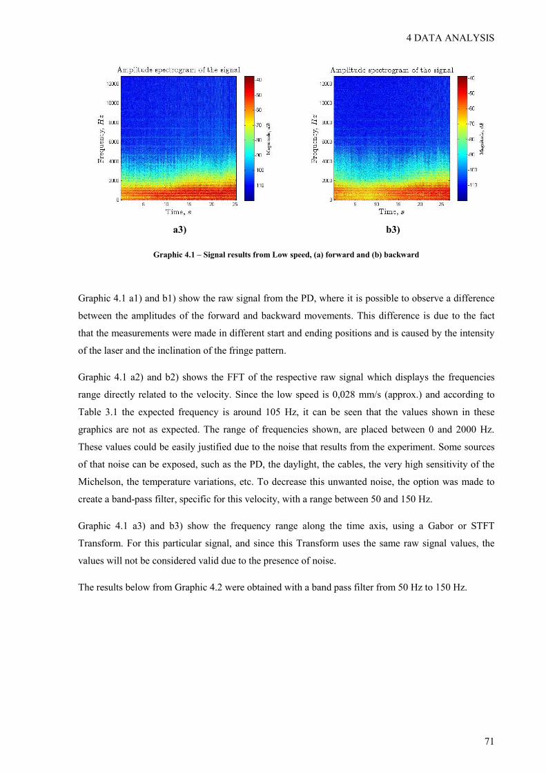
4 DATA ANALYSIS
71
a3) b3)
Graphic 4.1 – Signal results from Low speed, (a) forward and (b) backward
Graphic 4.1 a1) and b1) show the raw signal from the PD, where it is possible to observe a difference
between the amplitudes of the forward and backward movements. This difference is due to the fact
that the measurements were made in different start and ending positions and is caused by the intensity
of the laser and the inclination of the fringe pattern.
Graphic 4.1 a2) and b2) shows the FFT of the respective raw signal which displays the frequencies
range directly related to the velocity. Since the low speed is 0,028 mm/s (approx.) and according to
Table 3.1 the expected frequency is around 105 Hz, it can be seen that the values shown in these
graphics are not as expected. The range of frequencies shown, are placed between 0 and 2000 Hz.
These values could be easily justified due to the noise that results from the experiment. Some sources
of that noise can be exposed, such as the PD, the daylight, the cables, the very high sensitivity of the
Michelson, the temperature variations, etc. To decrease this unwanted noise, the option was made to
create a band-pass filter, specific for this velocity, with a range between 50 and 150 Hz.
Graphic 4.1 a3) and b3) show the frequency range along the time axis, using a Gabor or STFT
Transform. For this particular signal, and since this Transform uses the same raw signal values, the
values will not be considered valid due to the presence of noise.
The results below from Graphic 4.2 were obtained with a band pass filter from 50 Hz to 150 Hz.

4 DATA ANALYSIS
72
a1) b1)
a2) b2)
a3) b3)

4 DATA ANALYSIS
73
a4) b4)
a5) b5)
Graphic 4.2 – Signal results from Low speed, (a) forward and (b) backward with filter
Graphic 4.2 a1) and b1) show once again the raw signal from the PD. In these graphics, and
comparing with Graphic 4.1 a1) and b1), it is possible to understand that the signal obtained has less
frequencies, due to the filter used.
Graphic 4.2 a2) and b2) now show that it is possible to identify the expected frequency results around
the 100Hz, both for the forward and backward movements.
Graphic 4.2 a3) and b3) readily show an intense area of red color in the average of 100 Hz. It is almost
possible to draw a horizontal straight line in this value along the all-time of the movement, what
means that the driver has a constant velocity and the movement has not changed along the time the
signal was recorded.
According to the frequencies obtained in Graphic 4.2 a3) and b3) and to the relation between the
frequency and velocity from equation (2.66) Graphic 4.2 a4) and b4) was drawn, where the velocity
along the time is seen to be mostly constant as expected and in accordance with the theoretical values.
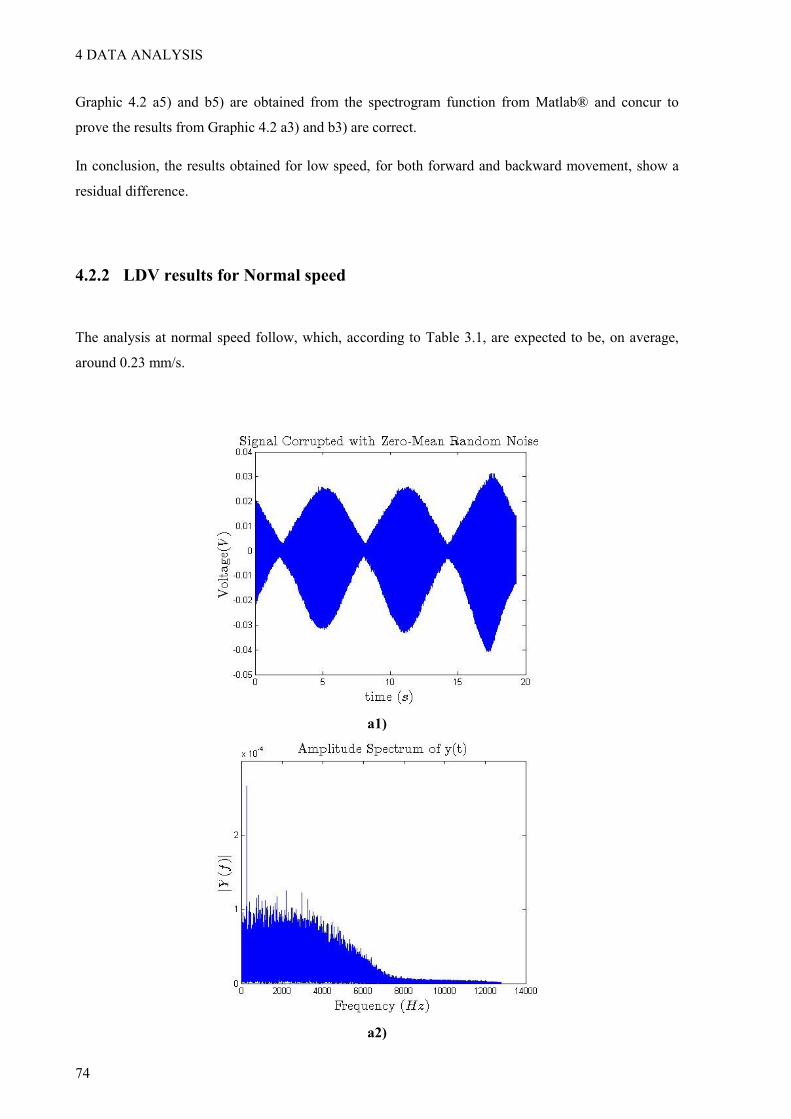
4 DATA ANALYSIS
74
Graphic 4.2 a5) and b5) are obtained from the spectrogram function from Matlab® and concur to
prove the results from Graphic 4.2 a3) and b3) are correct.
In conclusion, the results obtained for low speed, for both forward and backward movement, show a
residual difference.
4.2.2 LDV results for Normal speed
The analysis at normal speed follow, which, according to Table 3.1, are expected to be, on average,
around 0.23 mm/s.
a1)
a2)
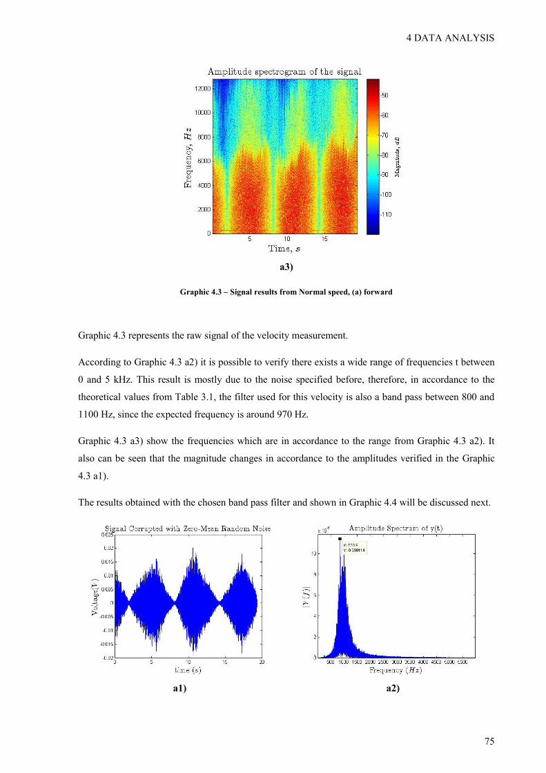
4 DATA ANALYSIS
75
a3)
Graphic 4.3 – Signal results from Normal speed, (a) forward
Graphic 4.3 represents the raw signal of the velocity measurement.
According to Graphic 4.3 a2) it is possible to verify there exists a wide range of frequencies t between
0 and 5 kHz. This result is mostly due to the noise specified before, therefore, in accordance to the
theoretical values from Table 3.1, the filter used for this velocity is also a band pass between 800 and
1100 Hz, since the expected frequency is around 970 Hz.
Graphic 4.3 a3) show the frequencies which are in accordance to the range from Graphic 4.3 a2). It
also can be seen that the magnitude changes in accordance to the amplitudes verified in the Graphic
4.3 a1).
The results obtained with the chosen band pass filter and shown in Graphic 4.4 will be discussed next.
a1) a2)

4 DATA ANALYSIS
76
a3) a4)
a5)
Graphic 4.4 – Signal results from Normal speed, (a) forward with filter
Graphic 4.4 a1) shows the raw signal from the PD. In this graphic, and comparing to Graphic 4.3 a1),
it is possible to understand that the signal obtained has less frequency peaks, due to the used filter.
In Graphic 4.4 a2) unlike the previous results, is possible to identify the expected results, with a
frequency around the 900 Hz, which is in accordance to the expected result.
An close look at Graphic 4.4 a3) shows that an intense area of red color in the average of 900 Hz is
clearly noticeable. These values prove there is a larger signal intensity for the frequencies around this
value, as expected. It is almost possible to draw a horizontal straight line in this value along the all-
time of the movement, which means that the driver has a constant velocity and the movement hasn’t
changed appreciably during the time span the signal was recorded. It is easily noticed that in this
imaginary horizontal line, there are some areas, in which the intensity decreases significantly.
Now, according to the frequencies obtained in Graphic 4.4 a3) and to the relation between the
frequency and velocity from equation (2.66) it is possible to draw Graphic 4.4 a4) where it can be seen
the velocity along the time axis, showing the velocity of the movement was nearly constant as
expected.
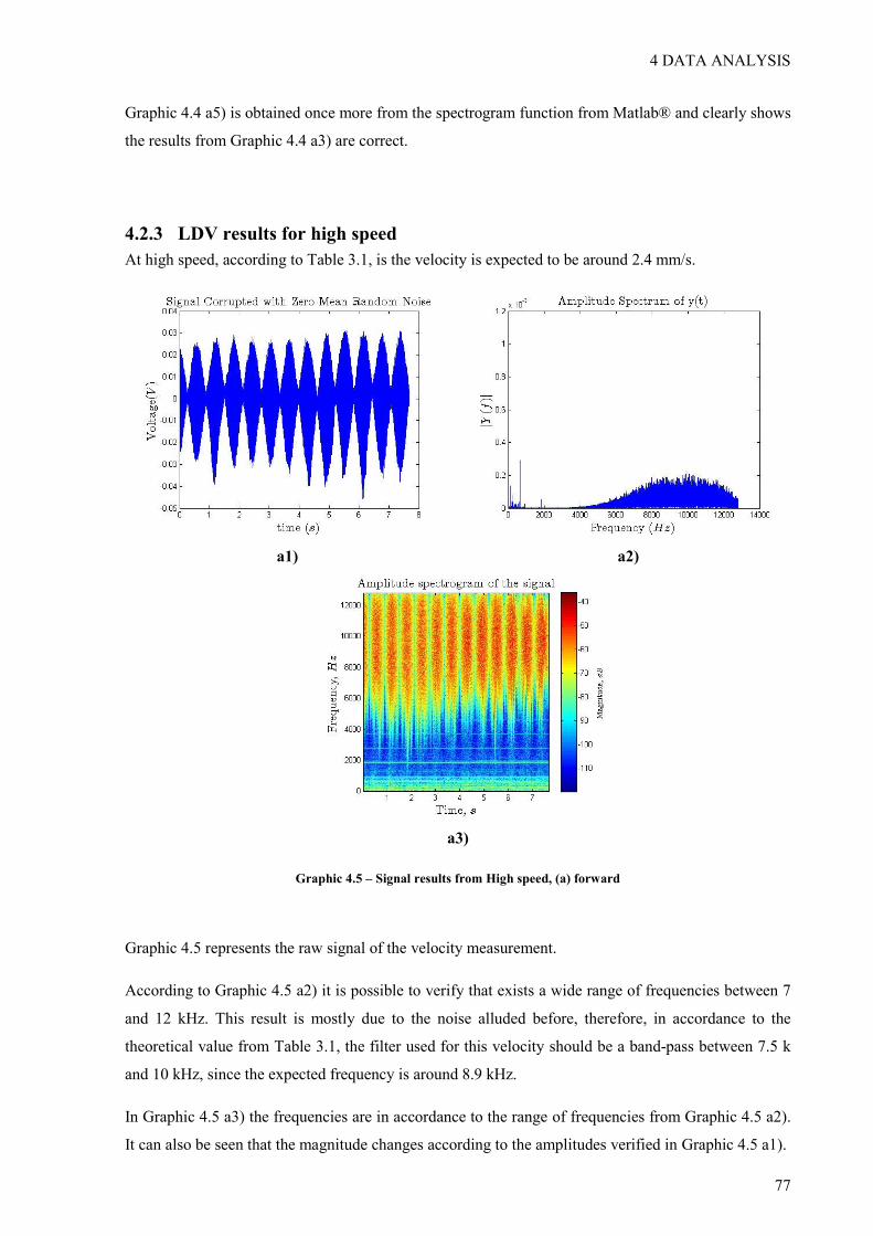
4 DATA ANALYSIS
77
Graphic 4.4 a5) is obtained once more from the spectrogram function from Matlab® and clearly shows
the results from Graphic 4.4 a3) are correct.
4.2.3 LDV results for high speed
At high speed, according to Table 3.1, is the velocity is expected to be around 2.4 mm/s.
a1) a2)
a3)
Graphic 4.5 – Signal results from High speed, (a) forward
Graphic 4.5 represents the raw signal of the velocity measurement.
According to Graphic 4.5 a2) it is possible to verify that exists a wide range of frequencies between 7
and 12 kHz. This result is mostly due to the noise alluded before, therefore, in accordance to the
theoretical value from Table 3.1, the filter used for this velocity should be a band-pass between 7.5 k
and 10 kHz, since the expected frequency is around 8.9 kHz.
In Graphic 4.5 a3) the frequencies are in accordance to the range of frequencies from Graphic 4.5 a2).
It can also be seen that the magnitude changes according to the amplitudes verified in Graphic 4.5 a1).
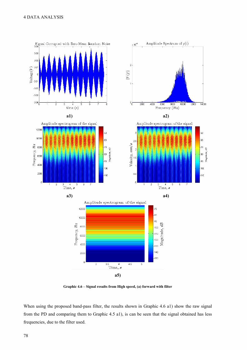
4 DATA ANALYSIS
78
a1) a2)
a3) a4)
a5)
Graphic 4.6 – Signal results from High speed, (a) forward with filter
When using the proposed band-pass filter, the results shown in Graphic 4.6 a1) show the raw signal
from the PD and comparing them to Graphic 4.5 a1), is can be seen that the signal obtained has less
frequencies, due to the filter used.

4 DATA ANALYSIS
79
In Graphic 4.6 a2) unlike the previous results, it is possible to identify the expected results, with a
frequency around the 9.8 kHz, which is proximate to the expected.
Doing an analysis at Graphic 4.6 a3) it is possible to notice the intense area of red color in the average
of 9.8 kHz. These values show a greater spectral power density of the frequencies around this value, as
expected. It is almost possible to draw a horizontal straight line in this value during the time of the
movement, which means that the driver has a constant velocity and the movement has not changed
during the time the signal was recorded. It is easily noticed that in the imaginary horizontal line, there
are some areas, in which the intensity decreases significantly. If analyzed in detail, these areas occur at
the same time where Graphic 4.6 a1) has an amplitude decrease.
Now, according to the frequencies obtained in Graphic 4.6 a3) and using the relation between the
frequency and velocity from equation (2.66) Graphic 4.6 a4) is calculated where it can be seen the
velocity along the time is mostly constant as expected from the theoretical values.
Graphic 4.6 a5) is obtained from the spectrogram function from Matlab® and shows the results from
Graphic 4.6 a3) are as expected.
Table 4.1 present the resume of all obtained values, with a comparison between the calculated
frequencies from the measured velocities and the obtained frequencies from the data analysis. In this
table are described all three measured velocities and the error between them. The error obtained it is
acceptable once the measured velocity is an approximation and also due to the noise of the
measurements.
Table 4.1 – Resume of the obtained values
Measured
Velocity [mm/s]
Calculated
Frequency [Hz]
Obtained
Frequency [Hz] Error %
Low Speed 0.028 105.28 78 25
Normal Speed 0.26 977.44 860 12
High Speed 2.348 8828 9800 11
4.2.4 Validation of the data
In order to validate the program made in Matlab® and to check if the PD was working as expected
frequency of the white fluorescent light in LOME was measured with the PD. This light is supposed to
have a frequency around 100 Hz.

4 DATA ANALYSIS
80
a1)
a2)

4 DATA ANALYSIS
81
a3)
a5)
Graphic 4.7 – Frequency from the white light source
Graphics 4.7 clearly testify the capability of the software tool used in performing data analysis proved
not only that the PD is collecting the right signal from the white light at the expected 100Hz, but also
that the signal treatment choices were the correct ones, as can be checked on the frequency plots and
the STFT spectrogram.
In Graphic 4.7 a2) the harmonics from this frequency happening in cycles of 100, i.e. 200 Hz, 300Hz,
etc. are also noticed and the intensity of these harmonics decreases with as expected also.

4 DATA ANALYSIS
82
The amplitude oscillation observed in the signal drawn in Graphic 4.7 a1) is due to the way that the
signal was acquired, by turning the PD directly into the laboratory lamp and recording the signal,
although this oscillation doesn’t really influence the frequency calculations to be performed
afterwards.
4.3 Results from PDV
In this section the data acquired with the RIGOL oscilloscope while measuring the velocity of the
Hopkinson input bar is analyzed. The output data from the oscilloscope is a CSV file that contains the
increments of the respective voltage values.
The parameters of the impact velocity measurements of the bar were established for a pressure of
approximately 3 bar. For the acquisition of the signal from PDV, it was necessary to use an external
trigger source, which was the signal from the strain gauges at the bar that is used to detect the sound
wave that travels in the bar after the impact.
It should be stressed that the longitudinal sound wave travels at a speed of approximately 5 Km/s in
the bar, a speed that is characteristic of the bar steel, whereas the bar itself moves at a pace of some 3
to 4 or 5 m/s, which is really the velocity that the PDV probe will measure as the reflector positioned
at the bar end moves away from it.
The first measurements were made with an impedance of 1 MΩ, with a sample rate of 2.5 GSa/s and
the voltage scale was 1 V per division, as shown in Figure 4.2.
The noisy strain gauge signal in blue shows the incident wave reaching the strain gauge at about 1ms
and moving away after some 800 s, at which time the signal from the PDV probe can be seen to start
its readouts, as set by the trigger.

4 DATA ANALYSIS
83
Figure 4.2 – Scope image from the first measurement
a) b)
Graphic 4.8 – Signal results from PDV for 1 MΩ
The signal in Graphic 4.8 a) is the output signal detected from the probe in yellow in yellow, where is
possible to say that the movement of the bar starts at nearly 2 ms and the frequency obtained after this
time is referred to the velocity of the bar.
To identify the velocity it is necessary to calculate the FFT of the signal and identify the main
frequency. According to Graphic 4.8 b) the FFT of the signal does not show any frequency, which
means that the oscilloscope could not detect any velocity during the measurement. The reason for this
is related with the overload of the oscilloscope in voltage values. Accordingly, the movement detected
in Graphic 4.8 a) is not the velocity of the bar but only noise detected by the probe.

4 DATA ANALYSIS
84
Since no results were obtained with oscilloscope in 1 MΩ, now data acquisition was performed with
an impedance of 50 Ω. The sample rate used was 50 MSa/s and the voltage scale was 2 mV per
division.
Graphic 4.9 – Signal results from PDV for 50 Ω
The Graphic 4.9 it is referred to the output signal detected from the probe.
Graphic 4.10 – FFT of the signal from PDV

4 DATA ANALYSIS
85
Graphic 4.10 represents the FFT of the signal obtained in Graphic 4.9. It is possible to identify the
main frequency of the movement and this frequency corresponds to 5 MHz. According to Eq. (2.66),
this frequency corresponds to a velocity of approximately 3.8 ms-1
which is found to agree with the
expected velocity of the bar.
PDV data analysis spectrogram could not be performed due to the fact that the power of the laser was
too low and the oscilloscope could not detect an effective frequency signal in time domain. The
Erbium Doped Fiber Amplifier which was ordered will increase the 5mW of the fiber laser to some
2.75dB or 500mW output power, clearly improving the laser performance and enabling noise reducing
strategies much more efficient.

4 DATA ANALYSIS
86

87
5 FUTURE WORK
Since this thesis appear through a work in progress from a FCT project, the project still has several
pending working subjects to go on. In this chapter it is described the future work that is still to be done
until the end of this project.
Also, as this thesis was taken up in LOME, it arose the need to develop a prototype of the LDV to
measure several velocities, from different applications and also the final PDV. Therefore, in this
chapter, it is also presented a proposal for a portable LDV and a PDV, that will be deployed as soon as
the LOME direction sees fit.
5.1 Future Work
The next step to do in this project is, as soon as the EDFA fiber amplifier arrives, is to insert it in the
PDV assembly and try to obtain some results about the range of velocities that the Hopkinson bar is
capable of.
The amplifier selected for the PDV was already referred in section 3.3 and is an EDFA Module from
NUPHOTONICS Technologies with the following specifications.
Features:
1540 – 1565 nm wavelength range;
+27 dBm output power provided for input power as low as +7 dBm;
+5 VDC powered EDFA Module;
The full specifications of the EDFA Module with all the mechanical drawings can be found in
Annex J.
5 FUTURE WORK
88
Figure 5.1 – EDFA Module Mechanical Drawing
Figure 5.2 – Detail of the amplifier inserted in the PDV
This amplifier will be connected between the laser diode and the port 1 of the circulator, as shown in
Figure 3.16 and in detail in Figure 5.2. With the amplifier setup, to have a PDV probe working
distance of nearly 20 mm is expected that should be enough to perform low-noise measurements of the
velocity at the Hopkinson bar.
Figure 5.3 – Final Scheme of the PDV adapted in Hopkinson bar

5 FUTURE WORK
89
After all the tests and acquisition of the data at the Hopkinson bar, the PDV will be adapted for the
electromagnetic forming, to measure the velocities that materials can achieve during the expanding
ring tests.
A second probe will be used to monitor deformation velocities in two directions.
In summary, a difficult ambitious project for the future awaits the conclusion of the first setup now
accomplished. Some critical situations will need to be carefully planned and scrutinized that have a
very short range for error accommodation. The aim of this future work is to create a clear link between
the high speed analysis and the material deformations, and also figure out how the direction of
measurement changes the frequencies, and how this relation is connected to the real speed of
deformation. The proposed objectives have a lot of concerns that cannot be answered now, and there is
still some uncertainty about the relation between the speed/frequencies measured in PDV and the
material deformation. For all explained, this will certainly be a very interesting project to be done in a
near future.
5.2 LDV Prototype
With the implementation of an LDV during the development of the current work, arouse the idea of
developing a portable LDV. The need of a LDV instrument in LOME emerged due to the fact that
there is no such equipment in the Laboratory, although the need to measure velocities is frequent.
The requirements for this LDV was to be portable and small and to be applied in different
applications, therefore it was designed to be very compact as per the scheme presented in Figure 5.4
Figure 5.4 – Scheme of the portable LDV

5 FUTURE WORK
90
The major difference between this portable LDV and the one developed in section 3.2 is the position
of the PD and M1. In order to make it more compact, the PD can be placed near the laser and the M3
can send the laser beam to the PD with the shifted frequency. M1 can be also placed on the other side
of the laser, once the path of the arms of the interferometer needs to be same, in the fixed arm is placed
a mirror M2. The arms of the interferometer need to be approximately the same length, to maintain the
coherence of the laser beam once the moving arm will increase or decrease the length of the respective
arm according to the reflective surface. As one of the requirements was the LDV to be used in the
most various applications, M1 can be adjusted so the length of the fixed arm is the same of the moving
one.
Figure 5.5 – Scheme of the portable LDV
The components of this LDV are the ones existing in LOME, the laser and the PD are the same used in
the LDV developed for this thesis and are placed in a small breadboard. Since the Michelson
interferometer is a very sensitive interferometer, the LDV needs to be placed inside a portable box.
This box, shown in Figure 5.6 has an aperture in the direction of the moving arm of the LDV. This gap
is used to protect the LDV inside the box and it is only open when there is the need to measure
velocities.

5 FUTURE WORK
91
Figure 5.6 – External appearance of the LDV
Figure 5.7 – Aspect of the LDV inside the box

5 FUTURE WORK
92

93
6 CONCLUSIONS
This dissertation work presents the development of a LDV for plastic deformation monitoring. Under
that assumption, the initial objectives were fulfilled, whereupon the implementation of a LDV was
completed and enabled the measurement of velocities. A PDV was also developed for higher-order
velocity measurements near to completion and already used for successfully measuring small speeds
in the SHPB, which is only limited by the lack of the laser amplifier for adequately reducing the noise
in the measurements. Finally a proposal for a portable LDV equipment was advanced and a prototype
was developed that LOME will be able to build in the future.
The initial work on a LDV assembly with a Mach- Zehnder interferometer and two Acousto-
Optic Modulators (AOM) served the instructive purpose of introducing the realm of the Doppler
Effect and its applications, thereby being adequate as an exploratory challenge where the moving
object would be replaced by the modulator and its artificially imposed Doppler shift. Inasmuch as the
plethora of laboratorial instrumentation and the AOM itself had to be used and therefore known to an
adequate extent, this initial work was in fact an opportunity for grasping the technicalities involved in
such assemblies. The fact the equipment was out of order and the AOMs didn’t modulate the input
light as expected, prevented the achievement of conclusive results, although the importance of this
initial setup really was to introduce the subject.
The following setup with a Michelson interferometer further extended the experience with laser
interferometers and the Doppler Effect. Michelson interferometers are very sensible devices and even
slight air movements could at times influence fringe stability. Further to that, setups with un-expanded
laser beams are difficult to control and align, even if the obtained fringes were relatively stable and
measurements could already be performed that were in full agreement with the theory, as expected.
Some measurement noise, most likely due to uncoupled electronic noise at the Photodetector perturbed
some of the measurements but still the discrepancy with the measured velocities was within acceptable
ranges, between 2 and 10%.
A Matlab program for evaluating the LDV and PDV results that read the data files, performed a
preliminary spectral analysis and thirdly performed a Power Spectral Density spectrogram analysis
was fully developed within the context of this work. A check of the obtained analysis results from the
6 CONCLUSIONS
94
known values of ordinary fluorescent light in the laboratory was performed with excellent results. This
software was really a necessity for analysing the signals from the photodetector and the PDV probe, as
there is no other expedite way to perform that analysis.
The setup of the all-fibre PDV device was straightforward and the device performs very well even
with a 5mW laser, showing a very good stability. The exploration of the device’s capabilities at high
and very high velocities with the fiber amplifier at nearly 500 mW laser output is greatly anticipated,
as is the possibility of measuring velocity along independent directions and checking the results.
The portable instrument design and development involved the laboratory people in order to
make it as compact as possible without losing the necessary flexibility to adapt to the requirements of
complex situations wherefore velocity measurements are necessary, albeit technically demanding. One
of the laboratory’s greatly appraised capabilities is the development of its own equipment whenever it
can’t be found in the commerce. Several pieces of equipment have been devised and built over the
years that fit into this reasoning, as does the proposed LDV.
In conclusion, the present work has been a rewarding one from different perspectives, because
of both their quality and the importance of their impact, clearly testifying to the high degree of
dedication and motivation along the entire work.

95
7 REFERENCES
1. Marciniak, Z., J.L. Duncan, and S.J. Hu, Mechanics of Sheet Metal Forming. 2002.
2. Nurcheshmeh, M., NUMERICAL PREDICTION OF SHEET METAL FORMING
LIMITS, in Electronic Theses and Dissertations2011, University of Windsor.
3. Stoughton, T.B. and X. Zhu, Review of theoretical models of the strain-based FLD
and their relevance to the stress-based FLD. International Journal of Plasticity, 2004.
20(8–9): p. 1463-1486.
4. Oliveira, I., et al., Study of strain-rate-dependent behavior of an aluminum alloy
during high speed loading, 2013: Germany.
5. Johnson, J.R., et al., Coupling Experiment and Simulation in Electromagnetic
Forming Using Photon Doppler Velocimetry. steel research international, 2009. 80(5):
p. 359-365.
6. Sargis, P.D., et al., Photonic Doppler Velocimetry, 1999, Lawrence Livermore
National Laboratory.
7. Oliveira, I.V.d., Electromagnetic forming process numerical modelling and analysis of
process parameters. 2013, Porto: FEUP. XVIII, 121 p.-XVIII, 121 p.
8. Rocha, A.B.d. and J.F. Duarte, Tecnologia da Embutidura. 1992.
9. Albrecht, H.E., et al., Laser Doppler and Phase Doppler Measurement Techniques.
2003.
10. Pain, H.J., The Physics of Vibrations and Waves. 6th ed. 2005.
11. McMillan, C.F., et al., Velocimetry of fast surfaces using Fabry–Perot interferometry.
Review of Scientific Instruments, 1988. 59(1): p. 1-21.
12. Reed, E.J., M. Soljačić, and J.D. Joannopoulos, Reversed Doppler Effect in Photonic
Crystals. Physical Review Letters, 2003. 91(13): p. 133901.
13. Moore, J.H., et al., Building Scientific Apparatus - A Practical Guide to Design and
Construction. Fourth Edition ed. 2009.
14. Hecht, E., Optics. Fourth Edition ed. 2002.
15. Hariharam, P., Basics of Interferometry. Second Edition ed. 2007.
16. Guenther, R.D., Modern Optics. 1990.
17. Sharma, K.K., Optics, Principles and applications. 2006.
18. Gasvik, K.J., Optical Metrology. Third Edition ed. 2002.
19. Sweatt, W.C., P.L. Stanton, and J.O.B. Crump. Simplified VISAR system. 1991.
20. Barker, L.M. and R.E. Hollenbach, Laser interferometer for measuring high velocities
of any reflecting surface. Journal of Applied Physics, 1972. 43(11): p. 4669-4675.
21. Dolan, D.H., Foundations of VISAR analysis, 2006, Sandia National Laboratories.
22. Buttler, W.T., et al., Optical Velocimetry. 2004.
23. Krauter, K. and S.O. Agbo, Single-mode VISAR: A Thesis. 2007: California
Polytechnic State University.
24. Strand, O.T., et al., Compact system for high-speed velocimetry using heterodyne
techniques. Review of Scientific Instruments, 2006. 77(8): p. 083108-083108-8.
7 REFERENCES
96
25. Weng, J., et al., Optical-fiber interferometer for velocity measurements with
picosecond resolution. Applied Physics Letters, 2006. 89(11): p. -.
26. Hemsing, W.F., Velocity sensing interferometer (VISAR) modification. Review of
Scientific Instruments, 1979. 50(1): p. 73-78.
27. Fleming, K.J. and T.A. Broyles, Shock Analysis Using the Multi Point Velocimeter
(VISAR), 2003, Sandia National Laboratories. p. 28.
28. Arrigoni, M., et al., Laser Doppler interferometer based on a solid Fabry–Perot
etalon for measurement of surface velocity in shock experiments. Measurement
Science and Technology, 2009. 20(1): p. 015302.
29. Tavares, P.J.d.S., Three-dimensional geometry characterization using structured light
fields. 2008, Porto: [s. n.]. XXX, 271, [2] p.-XXX, 271, [2] p.
30. Strand, O.T., et al. Velocimetry using heterodyne techniques. 2005.
31. Holtkamp, D.B. Survey of Optical Velocimetry Experiments - Applications of PDV, A
Heterodyne Velocimeter. in Megagauss magnetic field generation and related topics,
2006 ieee international conference on. 2006.
32. Kuznetsov, V.A. and S.P. Bennetts, Development of Photon Doppler Velocimeter for
Explosives Research, 2013, Australian Government Department of Defence - Defence
Science and Technology Organisation.
33. Press, W.H., Numerical recipes 3rd edition: The art of scientific computing. 2007:
Cambridge university press.
34. Casem, D.T. and M.B. Zellner, Kolsky Bar Wave Separation Using a Photon Doppler
Velocimeter. Experimental Mechanics, 2013. 53(8): p. 1467-1473.
35. Ferreira, F.J., Análise do comportamento dinâmico de componentes estruturais sob
solicitações generalizadas. 2003, Porto: [s. n.]. IIII, 231, [24] p.-IIII, 231, [24] p.
36. Avinadav, C., Y. Ashuach, and R. Kreif, Interferometry-based Kolsky bar apparatus.
Review of Scientific Instruments, 2011. 82(7): p. -.
37. Hotz, W., et al., Time Dependent FLC Determination Comparison of Different
Algorithms to Detect the Onset of Unstable Necking before Fracture. Key Engineering
Materials, 2013. Volume 549(Sheet Metal 2013): p. 397-404.

97
8 ANNEXES

8 ANNEXES
98
8.1 Annex A – Photo detector Data Sheet
8 ANNEXES
99

8 ANNEXES
100

8 ANNEXES
101

8 ANNEXES
102
8.2 Annex B – Determination of the velocities of the micro-positioner
Table 8.1 – Measurements of the velocity from the micro-positioner
Direction Distance Time Velocity
Distance Time Velocity
[mm] [s] [mm/s]
[mm] [s] [mm/s]
Forw
ard
10.0164 354.55 0.02825
10.0164 354.3 0.02827
9.991 357 0.02799
9.991 356.6 0.02802
9.9994 358.77 0.02787
9.9994 358.8 0.02787
10.0053 357.85 0.02796
10.0053 357.6 0.02798
10.0026 358.7 0.02789
10.0026 357.9 0.02795
Bac
kwar
d
10.0036 355.74 0.02812
10.0036 355.9 0.02811
10.0291 357.75 0.02803
10.0291 357.9 0.02802
10.0313 358.7 0.02797
10.0313 358.8 0.02796
10.0261 358.75 0.02795
10.0261 359.1 0.02792
10.0296 359.74 0.02788
10.0296 359.1 0.02793
Forw
ard
10.075 38.73 0.26013
10.075 38.9 0.25900
9.961 38.52 0.25859
9.961 38.1 0.26144
10.1382 38.96 0.26022
10.1382 39 0.25995
10.0436 38.59 0.26026
10.0436 38.7 0.25952
10.1256 38.76 0.26124
10.1256 39 0.25963
Bac
kwar
d
10.089 38.8 0.26003
10.089 39 0.25869
10.3399 39.61 0.26104
10.3399 39.9 0.25915
9.988 38.27 0.26099
9.988 38.2 0.26147
10.175 38.8 0.26224
10.175 38.5 0.26429
10.1611 39.06 0.26014
10.1611 39.3 0.25855
#DIV/0!
Forw
ard
10.3198 4.38 2.35612
10.3198 4.3 2.39995
10.2759 4.46 2.30401
10.2759 4.5 2.28353
10.9159 4.64 2.35256
10.9159 4.5 2.42576
10.1747 4.5 2.26104
10.1747 4.2 2.42255
10.8153 4.55 2.37699
10.8153 4.7 2.30113
Bac
kwar
d
10.2151 4.54 2.25002
10.2151 4.3 2.37560
11.0667 4.51 2.45381
11.0667 4.4 2.51516
10.2147 4.47 2.28517
10.2147 4.4 2.32152
9.3677 3.96 2.36558
9.3677 4 2.34193
10.342 4.11 2.51630
10.342 4.4 2.35045

8 ANNEXES
103
Table 8.2 – Standard Deviation of values from Table 8.2
Forward Backward
Low Velocity
Average 0,02800 0,02799 mm/s
Stand. deviation 0,00013 0,00007 (+/-) mm/s
Frequency Range
104,79 104,95 Hz
105,28 105,22 Hz
105,77 105,49 Hz
Normal Velocity
Average 0,26000 0,26066 mm/s
Stand. deviation 0,00080 0,00159 (+/-) mm/s
Frequency Range
974,42 973,94 Hz
977,44 979,92 Hz
980,46 985,90 Hz
High Velocity
Average 2,34836 2,37756 mm/s
Stand. deviation 0,05315 0,08207 (+/-) mm/s
Frequency Range
8628,62 8629,64 Hz
8828,44 8938,18 Hz
9028,26 9246,71 Hz
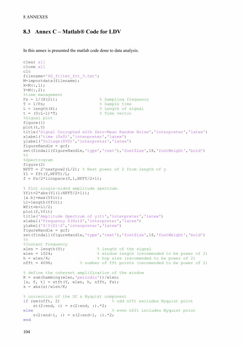
8 ANNEXES
104
8.3 Annex C – Matlab® Code for LDV
In this annex is presented the matlab code done to data analysis.
clear all
close all
clc
filename='HS_filter_frt_3.txt';
M=importdata(filename);
X=M(:,1);
Y=M(:,2);
%time management
Fs = 1/(X(2)); % Sampling frequency
T = 1/Fs; % Sample time
L = length(X); % Length of signal
t = (0:L-1)*T; % Time vector
%Signal plot
figure(1)
plot(t,Y)
title('Signal Corrupted with Zero-Mean Random Noise','interpreter','latex')
xlabel('time ($s$)','interpreter','latex')
ylabel('Voltage($V$)','interpreter','latex')
figureHandle = gcf;
set(findall(figureHandle,'type','text'),'fontSize',16,'fontWeight','bold')
%%
%Spectrogram
figure(2)
NFFT = 2^nextpow2(L/2); % Next power of 2 from length of y
Y1 = fft(Y,NFFT)/L;
f = Fs/2*linspace(0,1,NFFT/2+1);
% Plot single-sided amplitude spectrum.
Yfit=2*abs(Y1(1:NFFT/2+1));
[a b]=max(Yfit);
L1=length(Yfit);
Wfit=b+L1/2;
plot(f,Yfit)
title('Amplitude Spectrum of y(t)','interpreter','latex')
xlabel('Frequency $(Hz)$','interpreter','latex')
ylabel('$|Y(f)|$','interpreter','latex')
figureHandle = gcf;
set(findall(figureHandle,'type','text'),'fontSize',16,'fontWeight','bold')
%%
%Instant Frequency
xlen = length(Y); % length of the signal
wlen = 1024; % window length (recomended to be power of 2)
h = wlen/4; % hop size (recomended to be power of 2)
nfft = 4096; % number of fft points (recomended to be power of 2)
% define the coherent amplification of the window
K = sum(hamming(wlen,'periodic'))/wlen;
[s, f, t] = stft(Y, wlen, h, nfft, Fs);
s = abs(s)/wlen/K;
% correction of the DC & Nyquist component
if rem(nfft, 2) % odd nfft excludes Nyquist point
st(2:end, :) = s(2:end, :).*2;
else % even nfft includes Nyquist point
s(2:end-1, :) = s(2:end-1, :).*2;
end
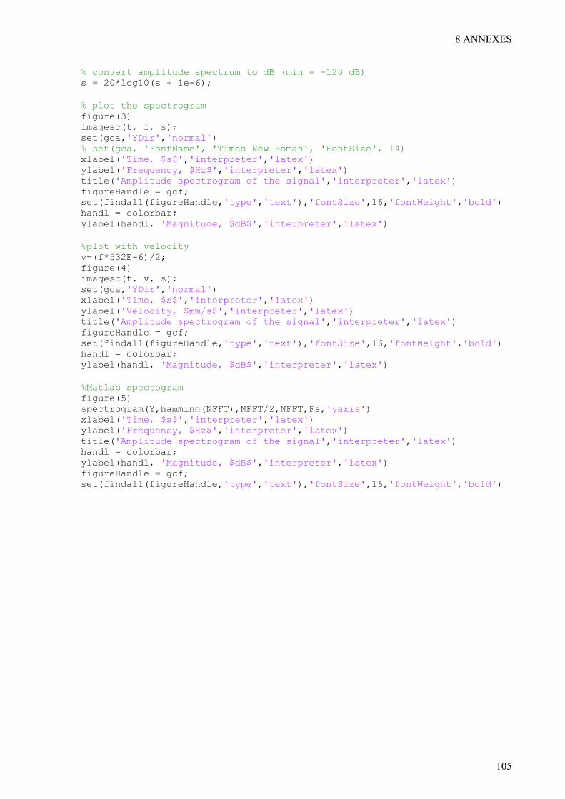
8 ANNEXES
105
% convert amplitude spectrum to dB (min = -120 dB)
s = 20*log10(s + 1e-6);
% plot the spectrogram
figure(3)
imagesc(t, f, s);
set(gca,'YDir','normal')
% set(gca, 'FontName', 'Times New Roman', 'FontSize', 14)
xlabel('Time, $s$','interpreter','latex')
ylabel('Frequency, $Hz$','interpreter','latex')
title('Amplitude spectrogram of the signal','interpreter','latex')
figureHandle = gcf;
set(findall(figureHandle,'type','text'),'fontSize',16,'fontWeight','bold')
handl = colorbar;
ylabel(handl, 'Magnitude, $dB$','interpreter','latex')
%plot with velocity
v=(f*532E-6)/2;
figure(4)
imagesc(t, v, s);
set(gca,'YDir','normal')
xlabel('Time, $s$','interpreter','latex')
ylabel('Velocity, $mm/s$','interpreter','latex')
title('Amplitude spectrogram of the signal','interpreter','latex')
figureHandle = gcf;
set(findall(figureHandle,'type','text'),'fontSize',16,'fontWeight','bold')
handl = colorbar;
ylabel(handl, 'Magnitude, $dB$','interpreter','latex')
%Matlab spectogram
figure(5)
spectrogram(Y,hamming(NFFT),NFFT/2,NFFT,Fs,'yaxis')
xlabel('Time, $s$','interpreter','latex')
ylabel('Frequency, $Hz$','interpreter','latex')
title('Amplitude spectrogram of the signal','interpreter','latex')
handl = colorbar;
ylabel(handl, 'Magnitude, $dB$','interpreter','latex')
figureHandle = gcf;
set(findall(figureHandle,'type','text'),'fontSize',16,'fontWeight','bold')
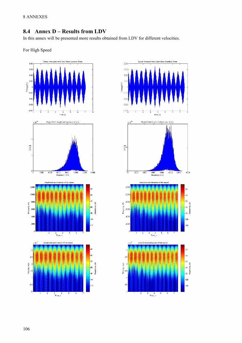
8 ANNEXES
106
8.4 Annex D – Results from LDV
In this annex will be presented more results obtained from LDV for different velocities.
For High Speed

8 ANNEXES
107
Normal Speed

8 ANNEXES
108
Low Speed

8 ANNEXES
109
8.5 Annex E – Matlab ® code for PDV
clear all; clc;
[filename, pathname] = uigetfile('*.csv', 'Pick a csv-file'); if isequal(filename,0) return; else File=fullfile(pathname, filename); end [pathstr, name, ext] = fileparts(File); M = csvread(File,2,0); t = M(:,1); V = M(:,2); t = t.*2E-8; Fs=2*10^abs(ceil(log10(t(2)-t(1)))); L=length(t); Lsq=2^nextpow2(L); %Next power of 2 from lenght of time vector - 65536*4; % f = Fs/2*linspace(0,1,Lsq/2+1); plot(t,V); % N = 12228; TF=fft(V,Lsq)/L; % ATF = fftshift(TF); figure; plot(f,2*abs(TF(1:Lsq/2+1))); xlabel('Freq (Hz)'); ylabel('|TF(f)|');
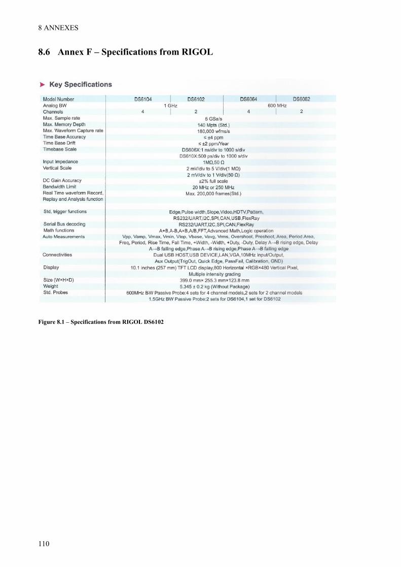
8 ANNEXES
110
8.6 Annex F – Specifications from RIGOL
Figure 8.1 – Specifications from RIGOL DS6102

8 ANNEXES
111
8.7 Annex G – Specifications from laser diode
Figure 8.2 – Calibration sheet of the laser diode
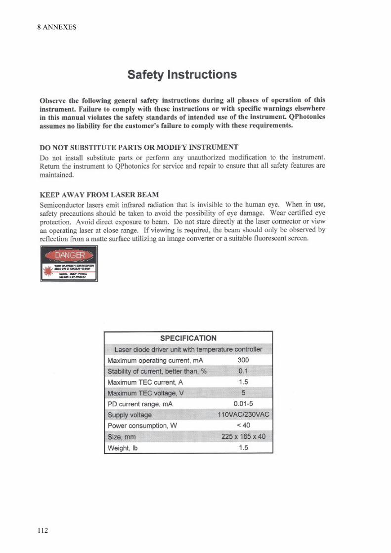
8 ANNEXES
112

8 ANNEXES
113

8 ANNEXES
114
8.8 Annex H – Specifications from detector

8 ANNEXES
115

8 ANNEXES
116

8 ANNEXES
117
8.9 Annex I – Specifications from fiber optical components
Figure 8.3 – Specifications of the Optical Circulator
Figure 8.4 – Specifications of the connector

8 ANNEXES
118
Figure 8.5 – Specifications of the probe

8 ANNEXES
119
8.10 Annex J – Specifications from EDFA Module amplifier
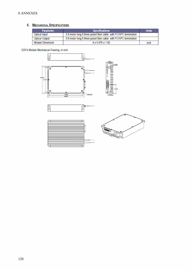
8 ANNEXES
120

8 ANNEXES
121
8.11 Annex K – LDV Prototype
In this annex are presented the different views of the Portable LVD protptype.
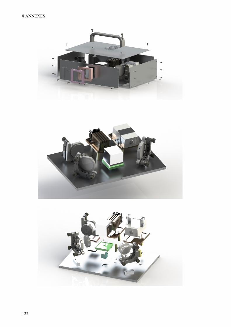
8 ANNEXES
122

8 ANNEXES
123