Development of a High Energy Resolution Gas Ionization ...
65
Development of a High Energy Resolution Gas Ionization Detector for a Recoil Spectrometer Jaakko Julin MSc thesis Pro gradu -tutkielma University of Jyv¨ askyl¨ a Department of Physics June 28, 2011 Supervisor: Timo Sajavaara
Transcript of Development of a High Energy Resolution Gas Ionization ...
Development of a High Energy Resolution Gas Ionization
Detector for a Recoil Spectrometer
Jaakko Julin
MSc thesis
Pro gradu -tutkielma
University of Jyvaskyla
Department of Physics
June 28, 2011
Supervisor: Timo Sajavaara

Abstract
In this thesis the development of a high energy resolution particle detector and
factors affecting the design of such a detector are explained. The particle detector
detects particles and measures the kinetic energy of the particle by means of collec-
ting the electrons liberated via ionization in the gaseous medium with an electric
field.
The goal of the detector development was to achieve better energy resolution than
a planar implanted silicon detector has for heavy ions. The gas ionization detector
forms a part of a time-of-flight energy telescope which is used as a recoil spectrome-
ter for Elastic Recoil Detection (ERD). The improved energy resolution improves
mass resolution of the telescope and allows heavier recoils to be separated.
Silicon detectors additionally suffer from energy resolution degradation when they
are bombarded by heavy ions. A gas ionization detector is radiation hard and the
gas can always be changed.
The detector developed at the JYFL accelerator laboratory uses a thin self-suppor-
ting silicon nitride entrance window to separate the isobutane used as the working
gas from the vacuum of the rest of the telescope. The window thickness (≤ 100 nm)
is crucial to the energy resolution for heavy recoils. Additionally the goal was to
have some position sensitivity to enable kinematic correction.
The ionization chamber was successfully designed and built and it achieved superior
mass resolution for all elements heavier than helium in comparison with the current
system, where a 450 mm2 Canberra PIPS silicon detector is used as the energy
detector.
i
Tiivistelma
Tassa tutkielmassa kuvataan kaasun ionisaatioon perustuvan korkean energiae-
rotuskyvyn hiukkasilmaisimen kehitystyo ja suunnitteluun vaikuttaneita tekijoita.
Kaasun ionisaatioon perustuva hiukkasilmaisin havaitsee ja mittaa hiukkasen liike-
energian keraamalla hiukkasen vapauttamat elektronit kaasusta sahkokentalla.
Tyon tarkoituksena oli saavuttaa parempi energiaerotuskyky kuin mihin pii-ilmai-
similla paastaan raskaille hiukkasille. Kaasuilmaisin toimii osana lentoaika-ener-
gia -spektrometria, jota kaytetaan Elastic Recoil Detection (ERD) mittauksiin.
Energiailmaisimen parempi energiaerotuskyky tarkoittaa parempaa spektrometrin
massaerotuskykya.
Pii-ilmaisimet karsivat lisaksi vaurioitumisesta hiukkaspommituksessa, mika joh-
taa entista huonompaan erotuskykyyn. Kaasun ionisaatioon perustuvat ilmaisimet
ovat sateilynkestavia ja kaasu voidaan aina tarvittaessa vaihtaa uuteen.
Jyvaskylan yliopiston kiihdytinlaboratoriossa kehitetyssa ilmaisimessa on ohut it-
sekantava piinitridikalvo ikkunana, joka erottaa kaasun spektrometrissa muuten
olevasta tyhjiosta. Ikkunan paksuus (≤ 100 nm) on oleellista raskaiden rekyylien
erotuskyvyn kannalta. Lisaksi tavoitteena oli saada ilmaisimesta paikkaherkka, mi-
ka mahdollistaa kinemaattisen korjauksen.
Kaasuilmaisin suunniteltiin ja rakennettiin onnistuneesti, ja silla saavutettiin pii-
ilmaisimeen nahden parempi massaresoluutio heliumia raskaammille rekyyleille
verrattuna nykyisin kaytossa olevaan spektrometriin, jossa energiailmaisimena on
450 mm2 Canberran PIPS pii-ilmaisin.
ii
Contents
1 Introduction 1
2 Interaction of energetic particles with matter 3
2.1 Particle energy loss . . . . . . . . . . . . . . . . . . . . . . . . . . . 3
2.2 Ionization . . . . . . . . . . . . . . . . . . . . . . . . . . . . . . . . 5
2.3 Straggling . . . . . . . . . . . . . . . . . . . . . . . . . . . . . . . . 6
3 Gaseous detectors 7
3.1 Gas ionization chambers . . . . . . . . . . . . . . . . . . . . . . . . 8
3.2 Detector physics . . . . . . . . . . . . . . . . . . . . . . . . . . . . . 8
3.2.1 Ionization . . . . . . . . . . . . . . . . . . . . . . . . . . . . 8
3.2.2 Charge collection and pulse formation . . . . . . . . . . . . . 9
3.2.3 Geometry . . . . . . . . . . . . . . . . . . . . . . . . . . . . 11
3.3 Gas and pressure . . . . . . . . . . . . . . . . . . . . . . . . . . . . 12
3.4 Entrance window . . . . . . . . . . . . . . . . . . . . . . . . . . . . 14
3.4.1 Silicon nitride windows . . . . . . . . . . . . . . . . . . . . . 14
3.5 Frisch grid . . . . . . . . . . . . . . . . . . . . . . . . . . . . . . . . 15
3.6 Electronics noise . . . . . . . . . . . . . . . . . . . . . . . . . . . . 18
3.7 Position sensitivity . . . . . . . . . . . . . . . . . . . . . . . . . . . 22
4 Elastic Recoil Detection 25
4.1 Time-of-flight ERD . . . . . . . . . . . . . . . . . . . . . . . . . . . 25
4.2 Kinematic correction . . . . . . . . . . . . . . . . . . . . . . . . . . 28
iii
5 The GIC built at JYFL Pelletron lab 29
5.1 Dimensions of the detector . . . . . . . . . . . . . . . . . . . . . . . 29
5.1.1 Range of recoils and scattered beam . . . . . . . . . . . . . 30
5.2 Vacuum and mechanical design . . . . . . . . . . . . . . . . . . . . 32
5.3 Electronics . . . . . . . . . . . . . . . . . . . . . . . . . . . . . . . . 34
5.3.1 Preamplifier . . . . . . . . . . . . . . . . . . . . . . . . . . . 34
5.3.2 Pulse shaping . . . . . . . . . . . . . . . . . . . . . . . . . . 36
5.3.3 Anode, cathode and grid voltages . . . . . . . . . . . . . . . 37
5.4 Frisch grid design and manufacturing . . . . . . . . . . . . . . . . . 39
5.5 Calibration and resolution . . . . . . . . . . . . . . . . . . . . . . . 41
5.5.1 Energy calibration . . . . . . . . . . . . . . . . . . . . . . . 41
5.5.2 Energy resolution . . . . . . . . . . . . . . . . . . . . . . . . 43
5.5.3 Mass resolution . . . . . . . . . . . . . . . . . . . . . . . . . 45
5.5.4 Position resolution . . . . . . . . . . . . . . . . . . . . . . . 51
5.6 Data aqcuisition and coincidence processing . . . . . . . . . . . . . 52
6 Conclusions 54
7 References 55
iv
1 Introduction
Elastic Recoil Detection (ERD) is an ion beam analysis method for quantitative
depth profiling of elemental composition in thin films. Originally ERD was done
with just an energy detector in the forward direction and absorber foils to suppress
incident beam [1] and was used for hydrogen detection in samples.
Today thin films of thickness 1-100 nm can be profiled typically with a resolution
of nearly 1 nm at the surface. Using more energetic incident beam samples can
be probed deeper, up to several µm [2], but often with reduced resolution. Heavy-
Ion ERD (HI-ERD) with heavier projectiles like 35Cl, 63Cu, 79Br, 127I or even197Au can be used to obtain depth profiles of not only the lighter elements but
of practically every element present in the samples, limited only by the mass or
elemental resolution of the spectrometer.
ERD requires not only energy spectrometry but particle identification for full ele-
mental analysis. The primary approaches to solve this problem are ∆E - E detec-
tors [3, 4], time-of-flight energy spectrometers (TOF-E) [5], magnetic spectrome-
ters [6,7] and Bragg ionization chambers [8] or other pulse shape methods [9]. Out
of the ion beam analysis methods ERDA is one of the more demanding in terms
of detector design. There is a need for simultaneous measurements of two or more
parameters of the recoiled particle such as its energy, energy loss, time of flight,
recoil angle, or charge to mass ratio.
Low energy heavy ion incident beams have a definite advantage over high energy
beams when it comes to depth profiling near the surface of the sample. Lower en-
ergy improves the obtained resolution with time-of-flight detectors. For a time-of-
flight measurement to be able to distinguish recoils with different mass the energy
of the particle needs to be measured. The relative energy resolution is decreased
for smaller energy recoils which combined with problems of energy measurement
of heavy recoils makes the mass separation more difficult. The capabilities of a
time-of-flight system are therefore not fully utilized until a high resolution energy
detector even for heavy recoils is introduced to the telescope. There still remains
room for improvement in the method, for example in obtaining isotopic composi-
tion or improving sensitivity.
1

Pelletron laboratory at JYFL Accelerator Laboratory has a Pelletron 5SDH-2 1.7
MV tandem accelerator with an RF source for 4He and sputtering source for heavy
ions. ERDA measurements are most often carried out with 5.1–6.8 MeV 35Cl and
6.8–10.2 MeV 79Br beams. The ≈ 2 MV accelerators are widely available and
are used for routine analysis of thin film samples, often for the semiconductor
industry. Other methods such as Rutherford Backscattering Spectrometry (RBS)
and Particle Induced X-ray Emission (PIXE) are used with 1-3 MeV 4He or 1H
beam with these accelerators. Some low energy TOF-ERD setups are in use [10–12]
and have shown their power in near surface depth profiling.
2
2 Interaction of energetic particles with matter
For the operation of a gas ionization chamber to be understood the basic principles
of radiation-matter interaction need to be reviewed. The main focus will be on
keV and MeV charged particles.
2.1 Particle energy loss
A charged particle will lose energy in a medium by several means. The main
interaction between the particle and matter is via Coulomb force due to fields
created by the particle and atoms of matter. Stopping is mostly due to inelastic
collisions between the particle and bound electrons of the matter but also due to
elastic collisions between nuclei. The latter effect will play a role at low energies,
typically near 10 to 100 keV. The effect of nuclear stopping is small, typically
under 1%, when the energy of the particle is above 200 keV/u [13]. Additionally
there can be excitations and radiative losses like bremsstrahlung. Stopping power
or stopping force is defined as
S(E) = −dEdx
= −(dE
dx nuclear+dE
dx electronic
). (1)
Here the total stopping force is written as a sum of the two main contributions.
The stopping force depends on the energy dramatically. Formulas and models have
been deviced to model this behaviour with a lot of work undertaken since the early
1900s. One of the most used formulas for energetic particles is the Bethe-Bloch
formula [14,15]
−dEdx
=4π
mec2· nz
2
β2·(
e2
4πε0
)2
·[ln
(2mec
2β2
I · (1− β2)
)− β2
], (2)
where β = vc, me mass of electron, n electron density of the matter, z charge state
of the particle, ε0 ionization energy ja c speed of light. What is relevant here is
the 1v2
dependence of stopping force to velocity of the particle.
For lower energies one needs to use other models. Often experimentalists rely on
semiempirical models such as the one used in Stopping and Range of Ions in Matter
3
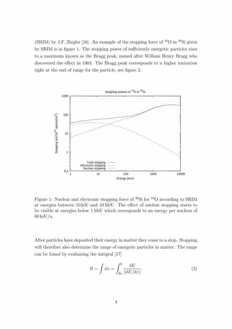
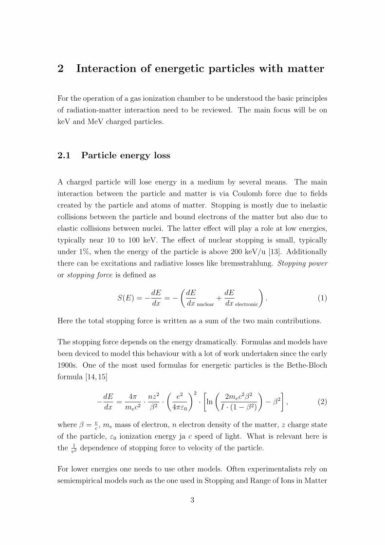
(SRIM) by J.F. Ziegler [16]. An example of the stopping force of 16O in 28Si given
by SRIM is in figure 1. The stopping power of sufficiently energetic particles rises
to a maximum known as the Bragg peak, named after William Henry Bragg who
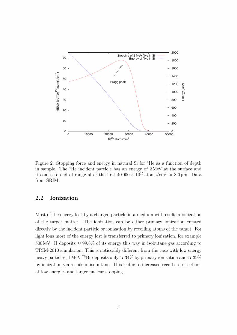
discovered the effect in 1903. The Bragg peak corresponds to a higher ionization
right at the end of range for the particle, see figure 2.
0.1
1
10
100
1000
1 10 100 1000 10000
Sto
ppin
g (e
V/1
015 a
tom
s/cm
2 )
Energy (keV)
Stopping powers of 16O in 28Si
Total stoppingElectronic stopping
Nuclear stopping
Figure 1: Nuclear and electronic stopping force of 28Si for 16O according to SRIMat energies between 10 keV and 10 MeV. The effect of nuclear stopping starts tobe visible at energies below 1 MeV which corresponds to an energy per nucleon of60 keV/u.
After particles have deposited their energy in matter they come to a stop. Stopping
will therefore also determine the range of energetic particles in matter. The range
can be found by evaluating the integral [17]
R =
∫dx =
∫ 0
E0
dE
(dE/dx). (3)
4
0
10
20
30
40
50
60
70
0 10000 20000 30000 40000 50000 0
200
400
600
800
1000
1200
1400
1600
1800
2000
-dE
/dx
(eV
/(10
15 a
tom
s)/c
m2 )
Ene
rgy
(keV
)
1015 atoms/cm2
Bragg peak
Stopping of 2 MeV 4He in SiEnergy of 4He in Si
Figure 2: Stopping force and energy in natural Si for 4He as a function of depthin sample. The 4He incident particle has an energy of 2 MeV at the surface andit comes to end of range after the first 40 000× 1015 atoms/cm2 ≈ 8.0 µm. Datafrom SRIM.
2.2 Ionization
Most of the energy lost by a charged particle in a medium will result in ionization
of the target matter. The ionization can be either primary ionization created
directly by the incident particle or ionization by recoiling atoms of the target. For
light ions most of the energy lost is transferred to primary ionization, for example
500 keV 1H deposits ≈ 99.8% of its energy this way in isobutane gas according to
TRIM-2010 simulation. This is noticeably different from the case with low energy
heavy particles, 1 MeV 79Br deposits only ≈ 34% by primary ionization and ≈ 39%
by ionization via recoils in isobutane. This is due to increased recoil cross sections
at low energies and larger nuclear stopping.
5
2.3 Straggling
A beam of particles slowing down in matter will introduce a spread in the beam
energy known as straggling. Stopping process is a statistical phenomenon and
therefore the energy of similar particles penetrating the same amount of matter
will always have a slightly different energy afterwards. Straggling will eventually
limit the energy and depth resolution of any ion beam analysis method.
The most used model for straggling is the Bohr theory, which assumes individual
collisions between particles and target electrons transfer small amount of the total
energy. This results in gaussian energy loss distribution [13].
At high energies electron excitations will introduce more straggling than predicted
by Bohr theory. At low energies charge exchange and effective charge of the pene-
trating particle have to be taken into account. The latter corrections are introduced
in the straggling models first by Chu [18] and Yang [19].
A spread of the ion tracks is also observed for particles, this is called lateral strag-
gling when it occurs in a direction parallel to the direction of the beam or range
straggling when it occurs in the same direction as the direction of the beam.
6
3 Gaseous detectors
Gas ionization chambers (GIC), ionization counters and other detectors that are
used to detect radiation by means of measuring ionization are collectively known
as gaseous detectors or simply gas detectors. Ionization chambers have been used
since the early days of nuclear and particle physics to detect and measure ionizing
particles [20]. First particle detectors such as the cloud chamber were impractical
for most measurements. Having a device like an ionization chamber which can be
used to detect radiation as an electrical signal was very useful.
Early gas ionization detector development was done in the 1940s and applied to
nuclear reaction studies. The single most important task was alpha spectroscopy.
Gas counters still find a role in the same field.
Gas detectors are nowadays very varied and are used to study radiation from a few
keV X-rays to several GeV energies of some particles. There has been significant
competition primarily from solid-state detectors, particularly silicon and germa-
nium detectors. Particle physics experiments have used gas detectors mostly out of
convenience as they are not damaged by highly energetic particles while providing
suitable medium for deceleration. Modern experiments like CMS and ATLAS at
CERN have shifted towards solid state silicon trackers and there has always been
competition from scintillation detectors for high energy calorimeters. Still such
detectors as Multi-Wire Proportional Chambers (MWPC), Drift Chambers, Time
Projection Chambers (TPC) and MicroStrip Gas Chambers (MSGC) are used to
measure the position of a particle [21] with good spatial and some temporal reso-
lution. In this sense they are used as particle trackers. Most of these designs are
absolutely unsuitable for low energy particle measurements, partially due to their
complexity and design relying on the fact that measured particles are minimum
ionizing particles (MIPs). Low energy ions would lose too much energy in the
wrong places of the detector. The physics which these detectors rely upon does
not always scale well. There has, however, been a lot of progress in this field of
gas detectors, compared with the relative inactivity in gas detector development
in other fields. There is something to be learned from the detector construction of
particle physics experiments even though the ideas wouldn’t be directly applicable.
7
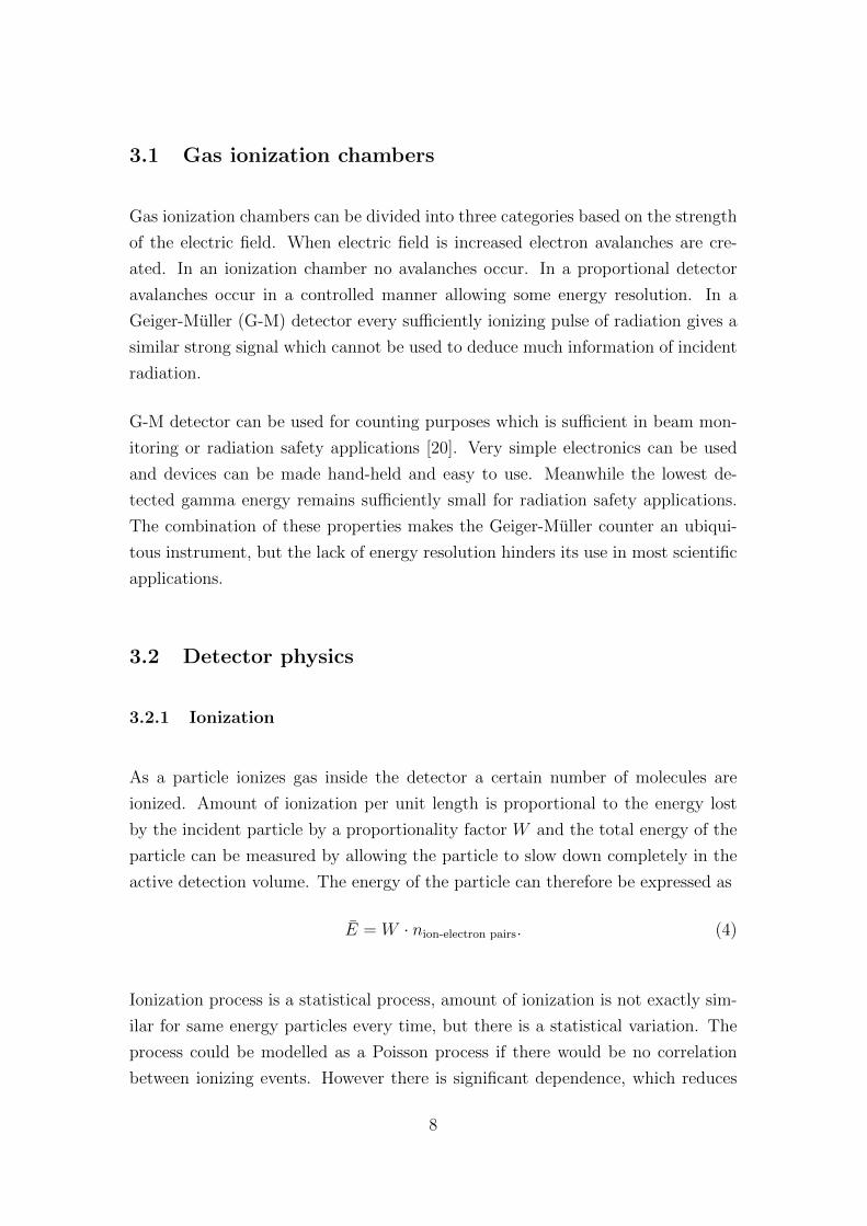
3.1 Gas ionization chambers
Gas ionization chambers can be divided into three categories based on the strength
of the electric field. When electric field is increased electron avalanches are cre-
ated. In an ionization chamber no avalanches occur. In a proportional detector
avalanches occur in a controlled manner allowing some energy resolution. In a
Geiger-Muller (G-M) detector every sufficiently ionizing pulse of radiation gives a
similar strong signal which cannot be used to deduce much information of incident
radiation.
G-M detector can be used for counting purposes which is sufficient in beam mon-
itoring or radiation safety applications [20]. Very simple electronics can be used
and devices can be made hand-held and easy to use. Meanwhile the lowest de-
tected gamma energy remains sufficiently small for radiation safety applications.
The combination of these properties makes the Geiger-Muller counter an ubiqui-
tous instrument, but the lack of energy resolution hinders its use in most scientific
applications.
3.2 Detector physics
3.2.1 Ionization
As a particle ionizes gas inside the detector a certain number of molecules are
ionized. Amount of ionization per unit length is proportional to the energy lost
by the incident particle by a proportionality factor W and the total energy of the
particle can be measured by allowing the particle to slow down completely in the
active detection volume. The energy of the particle can therefore be expressed as
E = W · nion-electron pairs. (4)
Ionization process is a statistical process, amount of ionization is not exactly sim-
ilar for same energy particles every time, but there is a statistical variation. The
process could be modelled as a Poisson process if there would be no correlation
between ionizing events. However there is significant dependence, which reduces
8
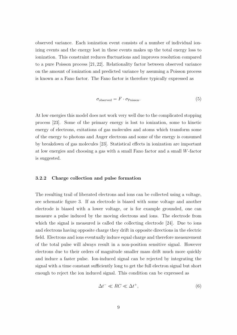
observed variance. Each ionization event consists of a number of individual ion-
izing events and the energy lost in these events makes up the total energy loss to
ionization. This constraint reduces fluctuations and improves resolution compared
to a pure Poisson process [21, 22]. Relationality factor between observed variance
on the amount of ionization and predicted variance by assuming a Poisson process
is known as a Fano factor. The Fano factor is therefore typically expressed as
σobserved = F · σPoisson. (5)
At low energies this model does not work very well due to the complicated stopping
process [23]. Some of the primary energy is lost to ionization, some to kinetic
energy of electrons, exitations of gas molecules and atoms which transform some
of the energy to photons and Auger electrons and some of the energy is consumed
by breakdown of gas molecules [23]. Statistical effects in ionization are important
at low energies and choosing a gas with a small Fano factor and a small W -factor
is suggested.
3.2.2 Charge collection and pulse formation
The resulting trail of liberated electrons and ions can be collected using a voltage,
see schematic figure 3. If an electrode is biased with some voltage and another
electrode is biased with a lower voltage, or is for example grounded, one can
measure a pulse induced by the moving electrons and ions. The electrode from
which the signal is measured is called the collecting electrode [24]. Due to ions
and electrons having opposite charge they drift in opposite directions in the electric
field. Electrons and ions eventually induce equal charge and therefore measurement
of the total pulse will always result in a non-position sensitive signal. However
electrons due to their orders of magnitude smaller mass drift much more quickly
and induce a faster pulse. Ion-induced signal can be rejected by integrating the
signal with a time constant sufficiently long to get the full electron signal but short
enough to reject the ion induced signal. This condition can be expressed as
∆t− RC ∆t+, (6)
9

where ∆t− is the electron collection time, ∆t+ is the ion collection time and RC
is the time-constant of the detector with resistance R of the signal plate of capac-
itance C to ground. By placing an AC-coupling capacitor and using a resistor to
ground or some DC high voltage this RC constant can be tuned. However this is
hardly practical and in practice filling the condition (6) might prove to be difficult
as the resistor value R needs to be high to reduce leakage current. This device
is called an electron-pulse chamber [24]. The fast pulse induced by electrons is
not only proportional to the charge but to the potential difference of the point of
ionization and collecting electrode [25]. This property can be exploited to achieve
position sensitive detectors, but it also complicates energy measurement.
Figure 3: Schematical picture of a pulse-mode parallel plate ionization chamberwhere the anode is biased and cathode grounded. Preamplifiers are AC coupled.
It is possible to achieve a signal proportional directly to the energy of the particle
by adding a grid of wires between electrodes which is biased to an appropriate
voltage between the electrode voltages. The induced charge from the motion of
electrons between one electrode and the grid is not induced to the other electrode,
but as electrons pass through the grid a signal is induced. The grid therefore shields
the collecting electrode. Now the potential difference of drifting charges seen by
the shadowed electrode remains constant and signal does not depend on the point
of ionization, but instead the full charge of ionization is collected. This grid is now
10
known as a Frisch grid, first implemented by Otto Frisch around 1940 [26]. It is
used in high resolution detectors with few exceptions.
Electric field strength is important in several ways. If no or very small voltage
is applied to the electrodes the opposite charges tend to recombine. Higher volt-
age will yield faster pulses which are typically preferred to achieve higher count
rates and reduce electron-ion recombination [21]. At some high electric field drift-
ing electrons will cause further ionization creating an effect known as electron
multiplication or at even higher voltage an avalanche. If amount of electron mul-
tiplication can be predicted with some accuracy this feature can be exploited to
have a better energy resolution due to smaller post-detector amplification. An un-
predictable avalanche of electrons is also useful if one doesn’t mind losing energy
resolution. To ion beam analysis energy proportionality is a minimum requirement
and operating in the avalanche region is unsought for. The highest obtainable en-
ergy resolution is possible only in the ionization region when both recombination
and multiplication are minimized. Only at the lowest energies where electronics
noise due to small amount of detected charges dominates there is an advantage of
the gas amplification, like in the case of GEM detectors [27].
3.2.3 Geometry
This far we have only concerned ourselves with planar geometry where the en-
trance window is in a parallel plane with the electrodes. Alternatively the window
could be in the same plane as the grid and electrodes, these detectors are either
transmission detectors such as position sensitive detectors (PSD) or some form of a
drift chamber. One very important geometry is the cylindrical detector which are
often used often in avalanche mode. The avalanche occurs near central wire, which
is chosen to be thin enough, typically between 20 and 100 µm diameter [21]. Due
to the shape of the electric field its density is highest near the wire. Cylindrical
ionization chambers do exist [28,29], in this case the wire is either thick or replaced
by a tube or there are wires in intermediate potential to reduce field density near
the anode and/or act as a Frisch grid. Cylindrical chambers also reject ion-induced
signal when chamber is operated in the ionization chamber mode. This is due to
logarithmic dependence on the distance of ionizing track to the signal induced on
the anode. If the central wire diameter is assumed to be 11000
of the cylinder diam-
11
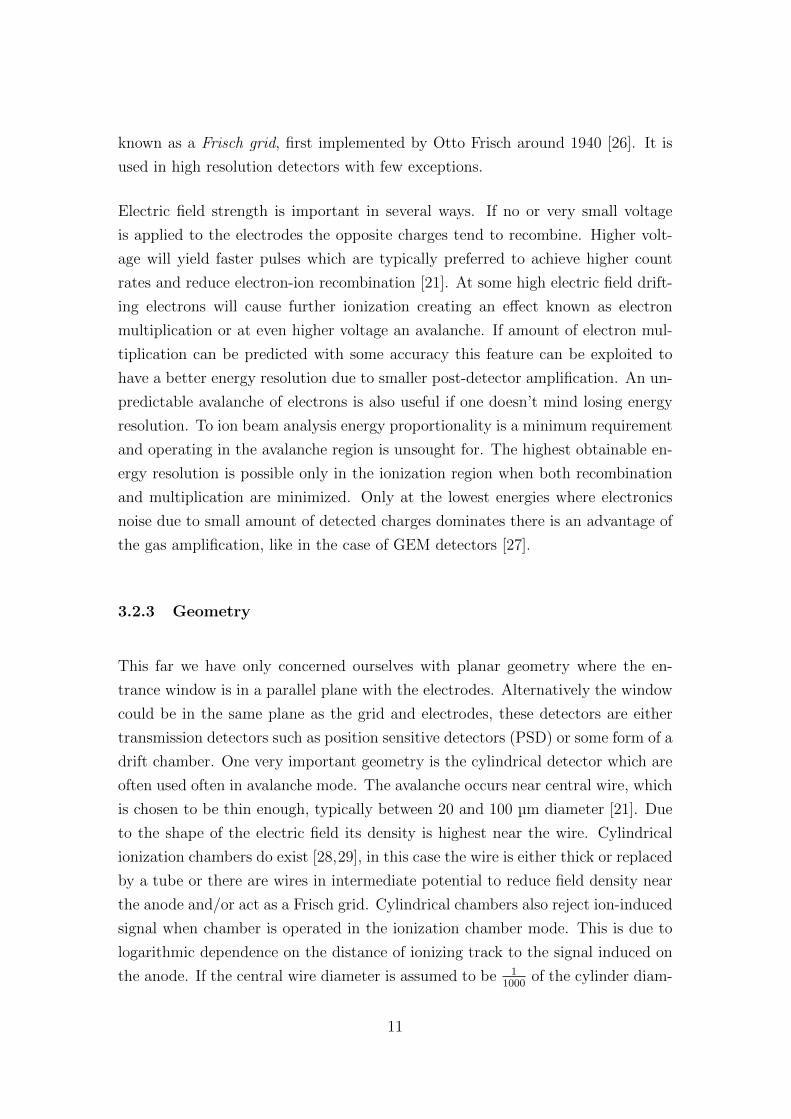
eter and the particle ionizes equidistant from anode and cathode the ion-induced
signal will be 10% of the electron-induced signal. A cylindrical ionization chamber
is presented schematically in figure 4.
Figure 4: Schematical picture of a cylindrical ionization chamber where the anodewire is biased and cathode grounded. Particles enter through a small window atthe end.
3.3 Gas and pressure
The choice of gas is not an obvious issue. The way the gas is chosen has been largely
based on experiments with different gases. A good detecting gas for an ionization
chamber most importantly needs to have a low ionization energy. This criteria is
met by most gases, the ionization energies vary between 20 and 40 eV. Refer to
section 3.2.1 on how the Fano factor is of signifigance to energy resolution. These
two factors are most critical, but there is also something to be won by choosing
a non-ideal gas, which is more dense than the ideal gas law would predict. These
gases stop particles in a shother distance for a given pressure. An example of such
gases are some organic gases such as isobutane or penthane. Heavy molecules will
anyway be more dense in the same pressure as light molecules.
12
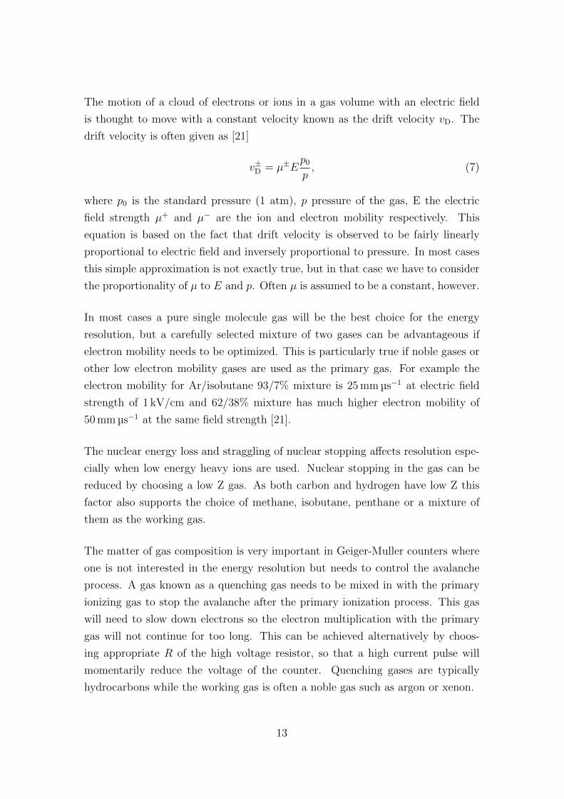
The motion of a cloud of electrons or ions in a gas volume with an electric field
is thought to move with a constant velocity known as the drift velocity vD. The
drift velocity is often given as [21]
v±D = µ±Ep0
p, (7)
where p0 is the standard pressure (1 atm), p pressure of the gas, E the electric
field strength µ+ and µ− are the ion and electron mobility respectively. This
equation is based on the fact that drift velocity is observed to be fairly linearly
proportional to electric field and inversely proportional to pressure. In most cases
this simple approximation is not exactly true, but in that case we have to consider
the proportionality of µ to E and p. Often µ is assumed to be a constant, however.
In most cases a pure single molecule gas will be the best choice for the energy
resolution, but a carefully selected mixture of two gases can be advantageous if
electron mobility needs to be optimized. This is particularly true if noble gases or
other low electron mobility gases are used as the primary gas. For example the
electron mobility for Ar/isobutane 93/7% mixture is 25 mm µs−1 at electric field
strength of 1 kV/cm and 62/38% mixture has much higher electron mobility of
50 mm µs−1 at the same field strength [21].
The nuclear energy loss and straggling of nuclear stopping affects resolution espe-
cially when low energy heavy ions are used. Nuclear stopping in the gas can be
reduced by choosing a low Z gas. As both carbon and hydrogen have low Z this
factor also supports the choice of methane, isobutane, penthane or a mixture of
them as the working gas.
The matter of gas composition is very important in Geiger-Muller counters where
one is not interested in the energy resolution but needs to control the avalanche
process. A gas known as a quenching gas needs to be mixed in with the primary
ionizing gas to stop the avalanche after the primary ionization process. This gas
will need to slow down electrons so the electron multiplication with the primary
gas will not continue for too long. This can be achieved alternatively by choos-
ing appropriate R of the high voltage resistor, so that a high current pulse will
momentarily reduce the voltage of the counter. Quenching gases are typically
hydrocarbons while the working gas is often a noble gas such as argon or xenon.
13
The gas should be of high purity to avoid impurities which could promote elec-
tron attachment and recombination. For example the mean time between electron
attachment in H2O is 140 ns and in O2 190 ns under normal conditions without
electric field [21].
High pressure gas will also stop particles in a shorter distance, giving reduced
straggling but higher ionization density. Large pressure can increase charge col-
lection time by reducing drift velocities of the electrons and reduce the efficiency
of charge collection via recombination. Higher electric field strength is needed to
compensate this.
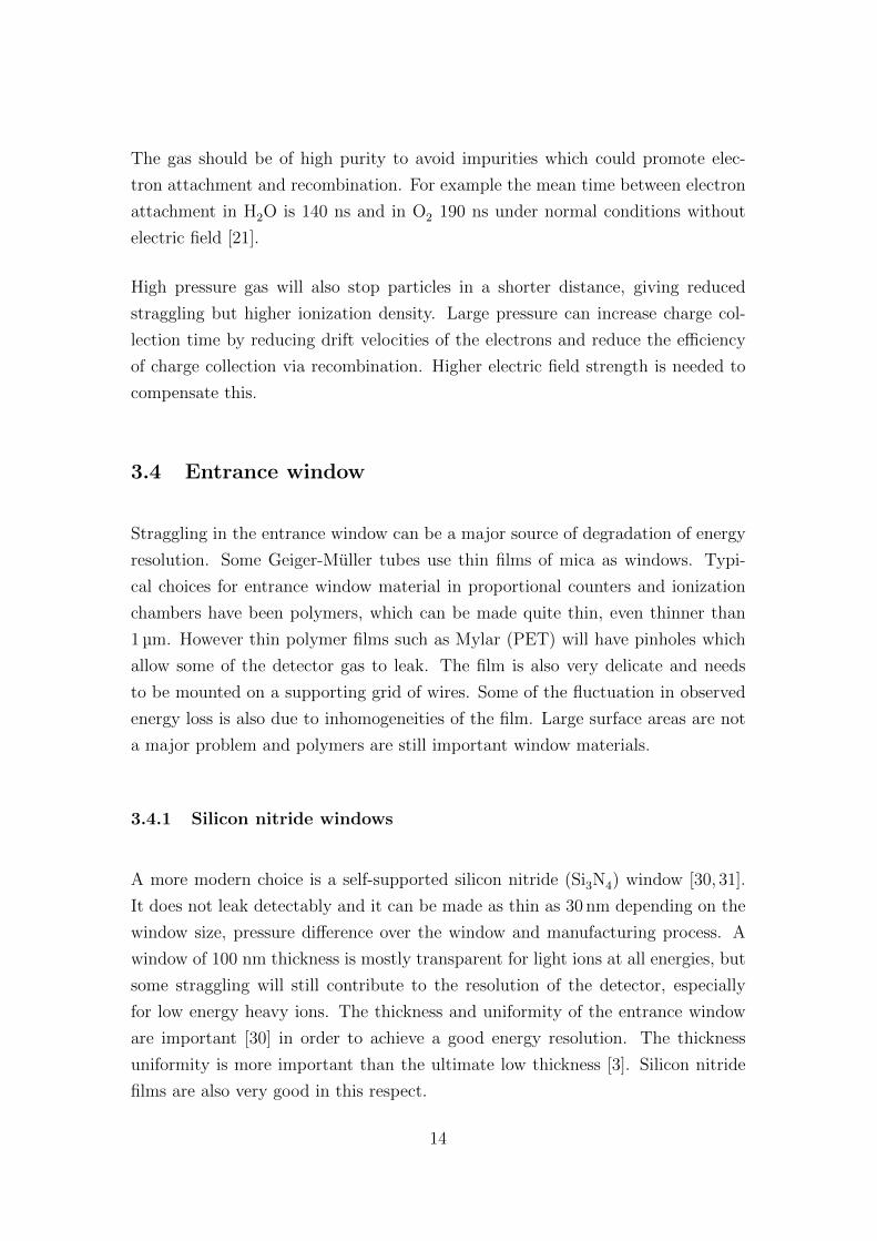
3.4 Entrance window
Straggling in the entrance window can be a major source of degradation of energy
resolution. Some Geiger-Muller tubes use thin films of mica as windows. Typi-
cal choices for entrance window material in proportional counters and ionization
chambers have been polymers, which can be made quite thin, even thinner than
1 µm. However thin polymer films such as Mylar (PET) will have pinholes which
allow some of the detector gas to leak. The film is also very delicate and needs
to be mounted on a supporting grid of wires. Some of the fluctuation in observed
energy loss is also due to inhomogeneities of the film. Large surface areas are not
a major problem and polymers are still important window materials.
3.4.1 Silicon nitride windows
A more modern choice is a self-supported silicon nitride (Si3N4) window [30, 31].
It does not leak detectably and it can be made as thin as 30 nm depending on the
window size, pressure difference over the window and manufacturing process. A
window of 100 nm thickness is mostly transparent for light ions at all energies, but
some straggling will still contribute to the resolution of the detector, especially
for low energy heavy ions. The thickness and uniformity of the entrance window
are important [30] in order to achieve a good energy resolution. The thickness
uniformity is more important than the ultimate low thickness [3]. Silicon nitride
films are also very good in this respect.
14

Silicon nitride film is deposited on both sides of a silicon wafer using Low Pressure
Chemical Vapor Deposition (LPCVD) from SiCl2H2 and NH3 precursors. Windows
are opened using for example Reactive Ion Etching (RIE) after which silicon is wet
etched from the openings, see figure 5. The remaining silicon nitride membrane is
self supporting and has low stress. These windows are available commercially for
example from Silson Ltd [32] in standard sizes up to a size of as 5 × 5mm2 and
with thicknesses of 30, 50, 100 nm and thicker. The current (June 2011) price for a
100 nm thick 5×5mm2 window is approximately 50 euros. Larger windows up to a
size of 20×20mm2 have been demonstrated. For detector purposes there is always
the option of using a matrix of windows. The only problem are the etched borders,
since the etching angle is only 55 degrees as determined by the silicon lattice. With
low energy heavy ion beams these are almost insignificant as the amount of silicon
needed to stop the particles is low. Still, some particles will traverse the silicon
through the etched borders and are a source of energy straggling. One can install
a carefully aligned collimator before the window to reduce this problem.
Figure 5: Cross section of a silicon wafer showing the etched shape.
3.5 Frisch grid
The Frisch grid has to shield the anode from the motion of electrons between the
grid and the cathode. Otherwise the signal will have some position sensitivity
which can not be easily corrected and will degrade energy resolution. The amount
of signal passing through is known as Frisch grid inefficiency (FGI) defined as σ in
equation 8. The actual measured anode pulse PmeasuredA can be written as [33]
PmeasuredA = P ideal
A + σ × P idealC , (8)
15
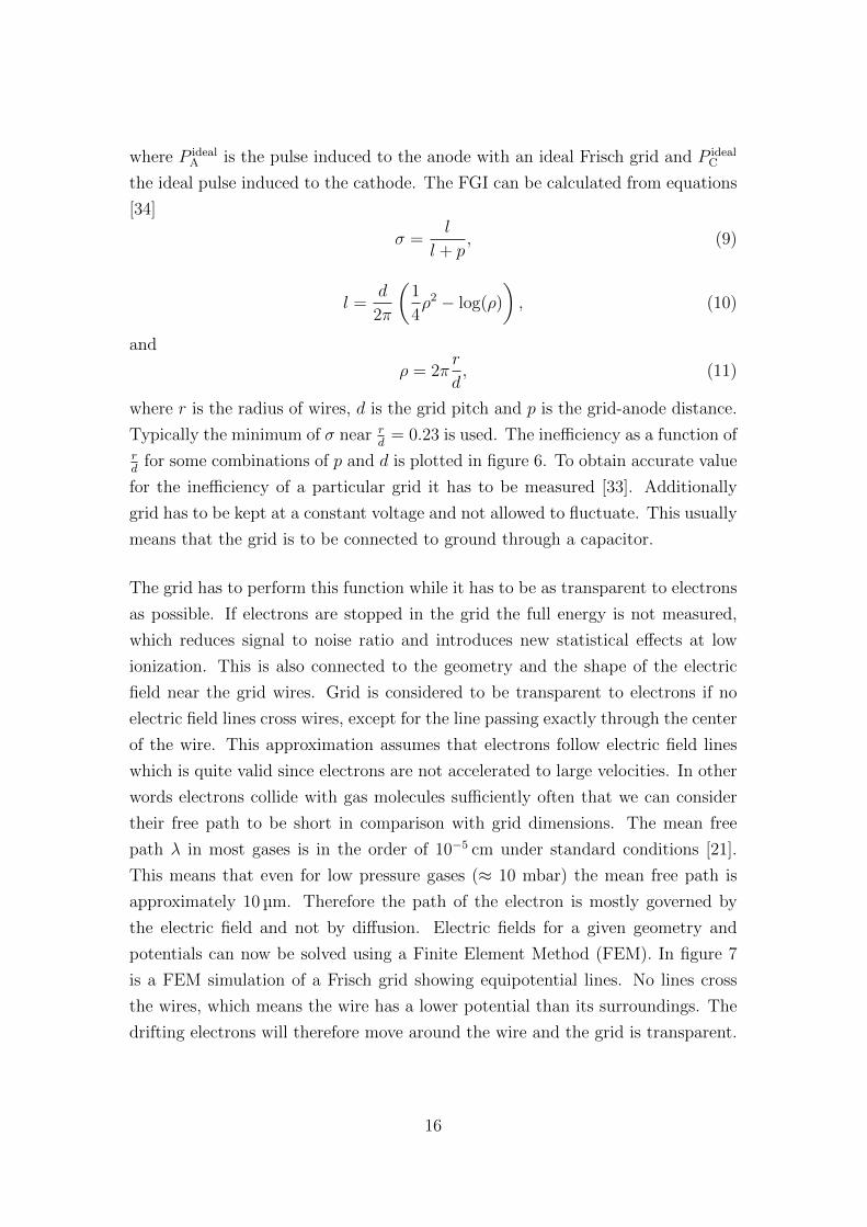
where P idealA is the pulse induced to the anode with an ideal Frisch grid and P ideal
C
the ideal pulse induced to the cathode. The FGI can be calculated from equations
[34]
σ =l
l + p, (9)
l =d
2π
(1
4ρ2 − log(ρ)
), (10)
and
ρ = 2πr
d, (11)
where r is the radius of wires, d is the grid pitch and p is the grid-anode distance.
Typically the minimum of σ near rd
= 0.23 is used. The inefficiency as a function ofrd
for some combinations of p and d is plotted in figure 6. To obtain accurate value
for the inefficiency of a particular grid it has to be measured [33]. Additionally
grid has to be kept at a constant voltage and not allowed to fluctuate. This usually
means that the grid is to be connected to ground through a capacitor.
The grid has to perform this function while it has to be as transparent to electrons
as possible. If electrons are stopped in the grid the full energy is not measured,
which reduces signal to noise ratio and introduces new statistical effects at low
ionization. This is also connected to the geometry and the shape of the electric
field near the grid wires. Grid is considered to be transparent to electrons if no
electric field lines cross wires, except for the line passing exactly through the center
of the wire. This approximation assumes that electrons follow electric field lines
which is quite valid since electrons are not accelerated to large velocities. In other
words electrons collide with gas molecules sufficiently often that we can consider
their free path to be short in comparison with grid dimensions. The mean free
path λ in most gases is in the order of 10−5 cm under standard conditions [21].
This means that even for low pressure gases (≈ 10 mbar) the mean free path is
approximately 10 µm. Therefore the path of the electron is mostly governed by
the electric field and not by diffusion. Electric fields for a given geometry and
potentials can now be solved using a Finite Element Method (FEM). In figure 7
is a FEM simulation of a Frisch grid showing equipotential lines. No lines cross
the wires, which means the wire has a lower potential than its surroundings. The
drifting electrons will therefore move around the wire and the grid is transparent.
16
Fris
ch g
rid in
effic
ienc
y
wire radius to grid pitch ratio
2.0 mm pitch 1 mm A−G distance1.0 mm pitch 1 mm A−G distance0.5 mm pitch 1 mm A−G distance2.0 mm pitch 8 mm A−G distance1.0 mm pitch 8 mm A−G distance0.5 mm pitch 8 mm A−G distance
0.001
0.01
0.1
1
0 0.1 0.2 0.3 0.4 0.5
Figure 6: Grid inefficiency σ as a function of the ratio of wire radius to grid spacingfor different combinations of grid anode-grid distance and wire spacing. Plottedusing equation (9).
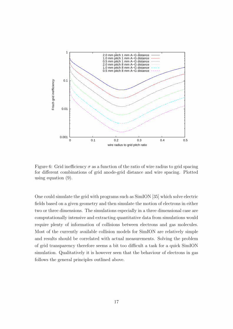
One could simulate the grid with programs such as SimION [35] which solve electric
fields based on a given geometry and then simulate the motion of electrons in either
two or three dimensions. The simulations especially in a three dimensional case are
computationally intensive and extracting quantitative data from simulations would
require plenty of information of collisions between electrons and gas molecules.
Most of the currently available collision models for SimION are relatively simple
and results should be correlated with actual measurements. Solving the problem
of grid transparency therefore seems a bit too difficult a task for a quick SimION
simulation. Qualitatively it is however seen that the behaviour of electrons in gas
follows the general principles outlined above.
17
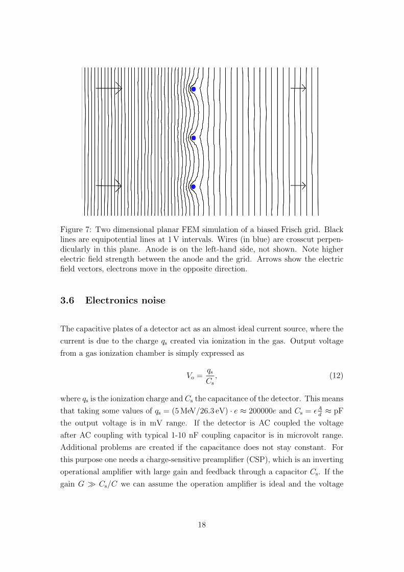
Figure 7: Two dimensional planar FEM simulation of a biased Frisch grid. Blacklines are equipotential lines at 1 V intervals. Wires (in blue) are crosscut perpen-dicularly in this plane. Anode is on the left-hand side, not shown. Note higherelectric field strength between the anode and the grid. Arrows show the electricfield vectors, electrons move in the opposite direction.
3.6 Electronics noise
The capacitive plates of a detector act as an almost ideal current source, where the
current is due to the charge qs created via ionization in the gas. Output voltage
from a gas ionization chamber is simply expressed as
Vo =qs
Cs
, (12)
where qs is the ionization charge and Cs the capacitance of the detector. This means
that taking some values of qs = (5 MeV/26.3 eV) · e ≈ 200000e and Cs = εAd≈ pF
the output voltage is in mV range. If the detector is AC coupled the voltage
after AC coupling with typical 1-10 nF coupling capacitor is in microvolt range.
Additional problems are created if the capacitance does not stay constant. For
this purpose one needs a charge-sensitive preamplifier (CSP), which is an inverting
operational amplifier with large gain and feedback through a capacitor Cs. If the
gain G Cs/C we can assume the operation amplifier is ideal and the voltage
18

output is now
Vo =qs
C. (13)
This means the capacitance of the detector itself does not affect the amplitude
of signal and the preamplifier acts as a charge integrator. The electronics noise
consists of two independent contributions, shot noise and thermal noise. The source
resistance and transresistance of the preamplifier create a contribution through
white spectrum of thermal noise which is due to kT energy of the electrons. The
other contribution, shot noise, is due to the charge qs consisting of a finite number
of electron charges. The standing currents at the preamplifier transistor fluctuate
as the number of actual charge carriers change. Both types of noise need to be
addressed, and typically noise is rejected by a band-pass filter which is combined
with an amplifier. This device is known as a spectroscopy amplifier. The frequency
at which the band-pass filter is centered is chosen with a shaping time τ . For a
more complete discussion on electronics noise see ref. [36].
The noise of the whole chain of electronics is expressed as the RMS deviation of
the detected charge. This number is typically gives as number of electrons and
known as Equivalent Noise Charge (ENC). The noise proportional to√τ is known
as parallel ENC and can be expressed as [36]
ENCP =Cse
G
√〈V 2〉P ≡ e
√τ
(kT
2Rs
+qIB
4
), (14)
where e is the Euler’s number, τ shaping time, IB current through base resistance
at the preamplifier or the drain current of a FET, q charge of the electron, Rs
preamplifier source resistance and 〈V 2〉P mean square voltage due to parallel noise
at the output.
The series noise due to shot noise is proportional to√
1/τ and given the transcon-
ductance gm of the preamplifier transistor can be expressed as [36]
ENCS =Cse
G
√〈V 2〉S ≡ eCs
√kT
2gmτ. (15)
From equations (14) and (15) one can observe that the series noise will dominate
as the detector capacitance increases, because the parallel noise is not dependent
19

on the capacitance at all. The transistor in the preamplifier itself acts as a source
of series noise as well. Thermal noise proportional to√kT is present in both
contributions. This means cooling of the transistor of the preamplifier is beneficial
as it reduces the thermal noise at the transistor and improves transconductance
gm, which futher reduces the series noise. Preamplifier RMS noise is given by the
manufacturers as a function of input capacitance, see figure 8 for the noise FWHM
as a function of input capacitance. This figure is easily reproduced if noise at zero
capacitance, i.e. parallel noise, is given, it is 0.67 keV FWHM for silicon detectors
at 2 µs shaping time, and if the noise slope (13 eVpF
) and capacitance (8 pF) of the
preamplifier transistor are given. The series and parallel noises are statistically
independent and can be summed quadratically
ENC =√
(ENCS)2 + (ENCP )2. (16)
The transistor capacitance Ct and the detector capacitance Cd can be summed to
give the total source capacitance since they can be treated as parallel capacitances.
The reproduction of the original figure based on these values is given in fig-
ure 9, but this time the vertical axis corresponds to FWHM assuming W =
26.3 eV/electron-ion -pair. The vertical axis is therefore scaled by 26.3 eV3.63 eV
. From
this image it is clear that the electronics noise is already a significant source of
error, considering this is a state-of-the-art preamplifier under ideal conditions. In
reality these values are difficult to achieve and therefore represent theoretical min-
ima. However, the effect of the input capacitance is fairly low in Amptek CoolFET
preamplifier, and should the detector capacitance be higher there is an alternative
FET with a higher capacitance, offering reduced noise slope. The drain current
of the FET can also be increased by changing the drain current resistor to reduce
noise slope by increasing transconductance. This will however increase the parallel
noise due to thermal noise.
The performance of a preamplifier with a specific detector can be tested by con-
necting the detector to the input of the preamplifier and feeding pulses from a
calibrated pulser. The test input is connected to the input of the FET of the
preamplifier similarly to the actual input. Alternatively the detector can be re-
placed by connecting an equivalent capacitance at the preamplifier input. Measur-
ing pulse height spectrum with an MCA and a spectroscopy amplifier will reveal
the actual RMS due to electronics. This procedure relies heavily on a good and
20
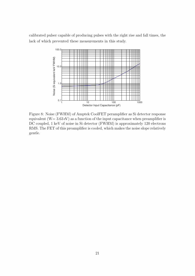
calibrated pulser capable of producing pulses with the right rise and fall times, the
lack of which prevented these measurements in this study.
Figure 8: Noise (FWHM) of Amptek CoolFET peramplifier as Si detector responseequivalent (W= 3.63 eV) as a function of the input capacitance when preamplifier isDC coupled, 1 keV of noise in Si detector (FWHM) is approximately 120 electronsRMS. The FET of this preamplifier is cooled, which makes the noise slope relativelygentle.
21

1
10
100
1 10 100 1000
Ele
ctro
nics
noi
se k
eV F
WH
M if
W=
26.3
eV
/pai
r
Detector capacitance (pF)
Electronics noise with Amptek CoolFET 8 pF FET
Figure 9: Amptek CoolFET RMS noise in keV FWHM as a function of the inputcapacitance, assuming W=26.3 eV/pair which corresponds to isobutane and valuesgiven for noise at zero capacitance and noise slope by the manufacturer.
3.7 Position sensitivity
Position sensitivity can be implemented in gas detectors using various techniques.
Most techniques give one dimensional position information and combination of two
different methods is typically used to achieve two dimensional position sensitivity.
Measuring pulses from an ungridded electrode to get a position and energy sensitive
information and from a gridded electrode in coincidence is simple and doesn’t affect
energy resolution. Position in the anode-cathode direction is obtained, but this
method is highly dependant on the shape of the electric field of the detector which
is typically non-ideal, especially in planar electrode gas ionization chambers.
One major problem in these detectors is the position sensitivity due entrance win-
dow aberrations [38]. If the entrance window is at ground potential ionization in
the first few millimeters of the active volume will not create ionization at the same
potential as in the rest of the detector. Deeper inside the detector closer to ideal
electric field is achieved, see also figure 10.
22

Figure 10: Two dimensional planar FEM simulation of fields near the entrancewindow in a plane perpendicular to the entrance window. The particles will enterthe gas volume from the left. Frisch grid (middle) is simulated as a plane. Entrancewindow is left out of the simulation, i.e. it is assumed to have a permittivity ofε0. Cathode (top) and the surroundings are assumed to be at ground potential.Entrance window aberrations are ample for this geometry but electrons shouldbe collected from near the window even if Frisch grid does not start immediatelyafter the window. The regions where the high electric field is strong, between theentrance window and the anode or the grid, should be void of free charges.
Another way is to split an electrode in two segments with a sawtooth-like pattern.
Higher signal will now induce to the segment closer to the ionization trail. If
one sums the signals the original energy signal is once again achieved. However
using two independent chains of electronics will result in summing of noise. Some
energy resolution will be lost if the split-electrode is the anode. It is also possible
to measure energy signal from a separate grid between anode and Frisch grid, but
this makes design more complicated. The advantage is that one does not need to
split the anode to obtain energy signal. Splitting the cathode is also an obvious
solution, but since particles create varying amount of ionization the resolution will
be degraded in the other end of the position spectrum.
23
Third way to implement position sensitivity is timing. For example in a typical
single grid detector where anode is shielded by the grid the charges drifting in
the gas begin to induce a signal to the anode much later than in the cathode.
Particles creating ionization near the grid will have short time difference between
the cathode and anode signals but particles ionizing closer to the cathode will
have longer time difference. Sources of error in measurement are similar to the
pulse-height comparing methods but differ in one key respect – timing signals are
mostly independent of the amount of ionization. Timing methods will yield a good
linear behaviour but are the most complicated to set up.
All these methods have been used successfully. Typical resolution obtained varies
between 1–5% depending on the method, implementation and solid angle of the
detector.
24
4 Elastic Recoil Detection
Elastic recoil detection is used to analyze a sample by means of impinging an ion
beam consisting of a single nuclide with well defined energy. Energy of the recoils
of mass M2 to an angle of φ with respect to the incident particle with mass M1
and energy E0 is
E2 = E04M1M2
(M1 +M2)2cos2 φ (17)
when the incident particles have an energy of E0 and mass M1. In most mea-
surements the φ is either assumed to be characteristic constant of the system or
measured for each particle. The incident beam is kept the same, which fixes the
value of M1. However due to stopping of the incident particles the E0 depends on
in which depth in the sample the recoil originates from.
At the sample surface E0 is known if the accelerator is calibrated correctly. This
allows us to predict the energies of the high energy edges. Detected recoils will also
have their energy reduced due to stopping in the sample. The distances particles
will have to travel can be altered by tilting the sample in respect to the incident
beam.
4.1 Time-of-flight ERD
A typical time-of-flight ERD telescope with two electrostatic mirror type timing
detectors with MCPs and the measurement geometry is drawn schematically in
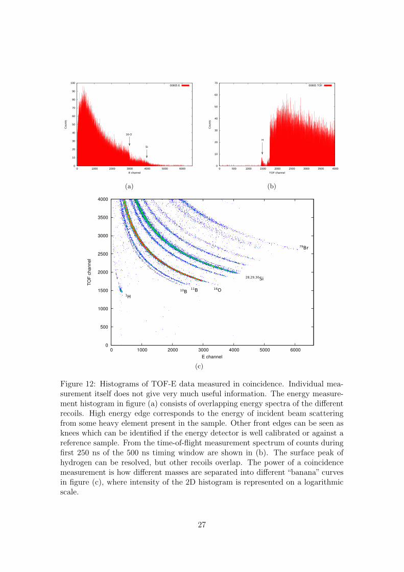
figure 11. Measuring simply the energy or velocity distribution of the recoiled ions
is not enough as one can see from figures 12(a) and 12(b). Different mass of recoils
means that energy spectra of recoils have significant overlapping. Measuring both
the time and energy in coincidence (figure 12(c)) will allow different masses to be
separated, since
m =2Ek
v2=
2Ek(L
t
)2 . (18)
25

Figure 11: Schematical picture of TOF-ERD telescope and measurement setupgeometry when sample surface is tilted to an angle of α with respect to the incidentbeam. The scattered incident beam and recoils are measured with the telescopeat an angle of φ with respect to the incident beam. Time of flight is measuredbetween the timing detectors T1 and T2 and energy of the particle with an energydetector, which can be either a silicon detector or a GIC. The particle is stoppedin the energy detector.
The mass resolution can be defined as
δm
m=
√√√√√(δE
E
)2
︸ ︷︷ ︸E detector
+
(2δL
L
)2
+
(2δt
t
)2
︸ ︷︷ ︸TOF detector
. (19)
Time of flight measurement is mostly independent of the species of the incident
particle and highly linear. The biggest contribution to the resolution is a simple
constant error δt coming from MCP timing properties and amplification and timing
electronics (CFD, TDC). The δt is typically between≈ 100−1000ps. Relative error
is highest for the most energetic particles because of δtt
term in it. This is in a stark
contrast with a gas detector or a silicon detector which have the lowest relative
error for energetic particles. It is therefore possible that highest energy resolution
is obtained with the energy detector for high-energy light particles. However the
very reliable energy calibration and worse resolution of the energy detector for
most particles tends to keep the TOF measurement as the preferred method for
energy measurement.
26
Cou
nts
E channel
16-O
Si
00805 E
0
10
20
30
40
50
60
70
80
90
100
0 1000 2000 3000 4000 5000 6000
(a)
Cou
nts
TOF channel
H
00805 TOF
0
10
20
30
40
50
60
70
0 500 1000 1500 2000 2500 3000 3500 4000
(b)
(c)
Figure 12: Histograms of TOF-E data measured in coincidence. Individual mea-surement itself does not give very much useful information. The energy measure-ment histogram in figure (a) consists of overlapping energy spectra of the differentrecoils. High energy edge corresponds to the energy of incident beam scatteringfrom some heavy element present in the sample. Other front edges can be seen asknees which can be identified if the energy detector is well calibrated or against areference sample. From the time-of-flight measurement spectrum of counts duringfirst 250 ns of the 500 ns timing window are shown in (b). The surface peak ofhydrogen can be resolved, but other recoils overlap. The power of a coincidencemeasurement is how different masses are separated into different “banana” curvesin figure (c), where intensity of the 2D histogram is represented on a logarithmicscale.
27
4.2 Kinematic correction
Position sensitivity in scattering plane allows one to implement a simple first-order
correction to tackle the problem of a finite detector size. In most experiments
scattering is considered to occur in a fixed scattering angle but a large detector
will naturally detect particles scattered to a range of scattering angles. Recoils to
smaller scattering angles will be more energetic than the ones to a larger scattering
angle as one can see from equation (17).
If straggling, multiple and plural scattering, and variations in the distance the
recoils travel in the sample are neglected the observed energy of the particle cor-
responds to a certain depth in the sample for a constant scattering angle. Now
when particles are measured scattering to a certain angle we can correct the energy
signal, so that it corresponds to an energy at the centerline scattering angle. The
result should be that energy signal corresponds to a single depth no matter what
scattering angle the particle is detected. The whole process is done as a linear
correction, which is not accurate for extremely large solid angles. However the
results are improved greatly comparing to a situation where detector solid angle is
simply approximated to be infinitely small.
It is also possible to calculate the true scattering angle from the position and use
that result in the analysis.
28
5 The GIC built at JYFL Pelletron lab
As an experimental part of this thesis a gridded planar geometry pulse-mode GIC
with a SiN entrance window was built. The detector was built to be mostly a
proof-of-concept but it is usable for some measurements, only limited by its rela-
tively small solid angle due to a small entrance window. It is possible to upgrade
the current detector by installing a larger window, at least 15× 15 mm2 should be
possible without other modifications to the detector. Mass resolution is slightly
worse than that obtained with a Si-detector for hydrogen, but already noticably
better for 10B at all energies. Mass resolution is good enough to separate even iso-
topes of silicon at higher energies, like with 10 MeV 79Br incident beam. Resolving10B from 11B or 11B from 12C is possible even for very low energy measurements
such as 3 MeV 35Cl incident beam.
5.1 Dimensions of the detector
A GIC for TOF-ERD has to be custom designed to suit the needs of a particular
TOF-setup. The energy range of measurement affects the range of ions in the gas
and that sets some geometrical constraints on the design. Maximum gas pressure,
entrance window thickness and detector geometry are all connected and much of
the design is set by attempting to optimize these parameters while keeping in mind
practical limitations.
There is not much generic data available of the pressure difference a silicon nitride
window can withstand as it depends on the manufacturing process of the silicon
nitride membrane. For the Silson Ltd manufactured 5 × 5 mm2 windows 100 nm
is enough to hold 200 mbar of pressure reliably, even a 50 nm window will hold
100 mbar [37]. A pressure of 100 mbar was the highest pressure these windows
were tested with in Jyvaskyla. Two 50 nm windows were also tested, the first one
was accidentally destroyed when glued to the window assembly and the other one
was destroyed by repeated pressure changes from vacuum to atmospheric pressure
or some other mechanical stress. It was decided based on the data from windows
made by Silson Ltd that 100 mbar should be the highest pressure used in the
detector ever.
29
The length of the active gas volume sets the maximum range detected particles
can have. The length of the anode will also increase the anode surface area and
therefore the detector capacitance and lateral straggling of the particles should also
be kept in mind. The anode can be cut if needed, so it was decided to have the
longest possible electrodes there is space for. This was 250 mm. Some more room
is required by an optional silicon detector which was used during the development
to detect e.g. particles not stopped in the gas.
Lateral dimensions were constrained by two choices. The biggest constraint was
that the detector was designed to be mountable either with anode/cathode plain
parallel or perpendicular to the scattering plane. This symmetry requires that the
active anode width is the same as anode-grid distance. The other limitation was
that the planar electrodes would have to fit in a round tube, which was easiest to
manufacture. Shoe-box style chambers are much more expensive and demanding
to manufacture. The active width and anode-grid distance was set at 40 mm due
to the limitations when 8 mm was reserved for the grid-anode distance, which was
set by Frisch grid design.
5.1.1 Range of recoils and scattered beam
The range of different recoils depends on their energy and stopping. Stopping can
be estimated for the highest energy recoils which have an energy given by formula
17. In figure 5.1.1 the tracks of particles with maximum energy given by 10.2
MeV 79Br and 8.5 MeV 35Cl incident beam for 41 degree recoil angle in 20 mbar
isobutane are simulated with SRIM. The increased energy of the heavier recoils is
opposed by the increased stopping power. The range of the particles of interest
recoiling from the surface is fairly similar for 79Br. For a lighter incident particle
such as 35Cl the lightest elements have the longest range.
The calculated ranges in 20 mbar of isobutane are all under 150 mm with less
than 10 mm FWHM of lateral straggling. This 10 mm margin means entrance
the side of the window needs to be 20 mm shorter than the grid-cathode distance.
Additional reduction is necessary to compensate for the geometric effects. As long
as entrance window effects are not of interest the range of particles can be tuned by
increasing the pressure. Allowing particles to stop just before the end of the anode
30
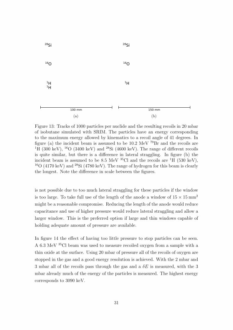
(a) (b)
Figure 13: Tracks of 1000 particles per nuclide and the resulting recoils in 20 mbarof isobutane simulated with SRIM. The particles have an energy correspondingto the maximum energy allowed by kinematics to a recoil angle of 41 degrees. Infigure (a) the incident beam is assumed to be 10.2 MeV 79Br and the recoils are1H (300 keV), 16O (3400 keV) and 28Si (4600 keV). The range of different recoilsis quite similar, but there is a difference in lateral straggling. In figure (b) theincident beam is assumed to be 8.5 MeV 35Cl and the recoils are 1H (530 keV),16O (4170 keV) and 28Si (4780 keV). The range of hydrogen for this beam is clearlythe longest. Note the difference in scale between the figures.
is not possible due to too much lateral straggling for these particles if the window
is too large. To take full use of the length of the anode a window of 15× 15 mm2
might be a reasonable compromise. Reducing the length of the anode would reduce
capacitance and use of higher pressure would reduce lateral straggling and allow a
larger window. This is the preferred option if large and thin windows capable of
holding adequate amount of pressure are available.
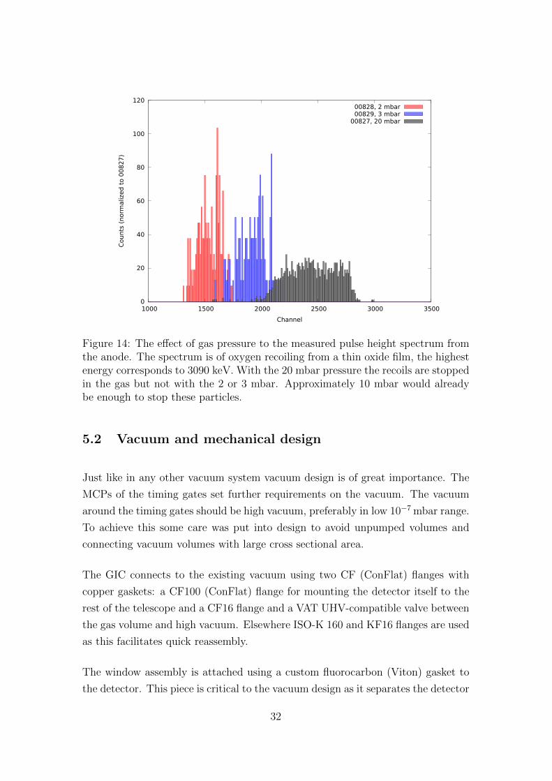
In figure 14 the effect of having too little pressure to stop particles can be seen.
A 6.3 MeV 35Cl beam was used to measure recoiled oxygen from a sample with a
thin oxide at the surface. Using 20 mbar of pressure all of the recoils of oxygen are
stopped in the gas and a good energy resolution is achieved. With the 2 mbar and
3 mbar all of the recoils pass through the gas and a δE is measured, with the 3
mbar already much of the energy of the particles is measured. The highest energy
corresponds to 3090 keV.
31
Counts
(norm
aliz
ed
to 0
08
27
)
Channel
00828, 2 mbar00829, 3 mbar
00827, 20 mbar
0
20
40
60
80
100
120
1000 1500 2000 2500 3000 3500
Figure 14: The effect of gas pressure to the measured pulse height spectrum fromthe anode. The spectrum is of oxygen recoiling from a thin oxide film, the highestenergy corresponds to 3090 keV. With the 20 mbar pressure the recoils are stoppedin the gas but not with the 2 or 3 mbar. Approximately 10 mbar would alreadybe enough to stop these particles.
5.2 Vacuum and mechanical design
Just like in any other vacuum system vacuum design is of great importance. The
MCPs of the timing gates set further requirements on the vacuum. The vacuum
around the timing gates should be high vacuum, preferably in low 10−7 mbar range.
To achieve this some care was put into design to avoid unpumped volumes and
connecting vacuum volumes with large cross sectional area.
The GIC connects to the existing vacuum using two CF (ConFlat) flanges with
copper gaskets: a CF100 (ConFlat) flange for mounting the detector itself to the
rest of the telescope and a CF16 flange and a VAT UHV-compatible valve between
the gas volume and high vacuum. Elsewhere ISO-K 160 and KF16 flanges are used
as this facilitates quick reassembly.
The window assembly is attached using a custom fluorocarbon (Viton) gasket to
the detector. This piece is critical to the vacuum design as it separates the detector
32

Figure 15: Mechanical construction of the developed GIC.
gas volume from the high vacuum present elsewhere in the detector telescope. The
pressure difference between the detector volume and high vacuum will tend to push
the window assembly outwards. The windows assembly has 16 M3 screws to ensure
an even and a tight fit, but in reality 8 screws was more than enough. Weldments
obviously need to be done with regular vacuum weld techniques. Material choices
were mostly unaffected, although the use of epoxy is not recommended as this will
increase pumping time significantly. There are alternatives to regular epoxy such
as Varian Torr Seal, which is good for pressure as low as 1× 10⁻⁹ mbar.
However in everyday use the gas handling turned out to be easy. When the detector
is first installed some pumping time should be allowed. As the pressure decreases
the detector is ready for the gas. The valve connecting the detector gas volume to
the vacuum is closed. When some gas is now introduced to the detector extremely
carefully one can observe the status of the entrance window indirectly by observing
the pressure of the vacuum. If there is no change the window is intact and will
hold more pressure. Pressure can be carefully increased to final pressure. When
measurements are over the gas can be rough-pumped away, time-of-flight detector
33
high voltage is turned off and the valve to the gas volume can be opened gently.
The remaining pressure is still high enough to trigger vacuum interlocks if care is
not taken. Repeating the gas handling procedure is only necessary about once per
day, and only takes a minute or two. The gas handling is the only increased effort
from users point of view when comparing to a solid-state detector.
5.3 Electronics
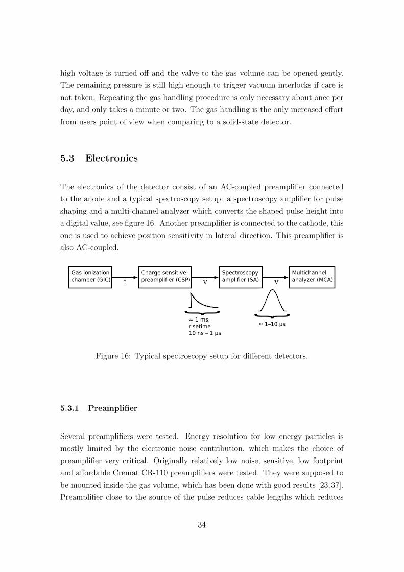
The electronics of the detector consist of an AC-coupled preamplifier connected
to the anode and a typical spectroscopy setup: a spectroscopy amplifier for pulse
shaping and a multi-channel analyzer which converts the shaped pulse height into
a digital value, see figure 16. Another preamplifier is connected to the cathode, this
one is used to achieve position sensitivity in lateral direction. This preamplifier is
also AC-coupled.
Figure 16: Typical spectroscopy setup for different detectors.
5.3.1 Preamplifier
Several preamplifiers were tested. Energy resolution for low energy particles is
mostly limited by the electronic noise contribution, which makes the choice of
preamplifier very critical. Originally relatively low noise, sensitive, low footprint
and affordable Cremat CR-110 preamplifiers were tested. They were supposed to
be mounted inside the gas volume, which has been done with good results [23,37].
Preamplifier close to the source of the pulse reduces cable lengths which reduces
34
electronics noise by avoiding stray capacitance and EM pickup. The development
of the detector with custom electronics is a demanding task, so the idea was aban-
doned for now. Self-made PCB boards with CR-110 preamplifiers proved relatively
successful, noise performance was on par with factory assembled Cremat pream-
plifiers.
Further improvement was sought with an Amptek CoolFET preamplifier, the noise
performance of which is state-of-the-art due to a Peltier-cooled field effect transis-
tor. Cooling of the FET reduces thermal noise and improves the transconductance
of the FET. The low frequency noise of the detector proved to be a problem with
both the CR-110 and CoolFET with a protection diode installed. This noise is
present as a difference in the DC level between two pulses in figure 17. The best
performance was achieved with Ortec 142 -series preamplifiers, with both 142A and
142B achieving nearly identical noise performance. The 142A is intended for lower
capacitance detectors and has higher conversion gain, which is an advantage since
measured pulses are small. Since all tested preamplifiers have a similar operating
principle and only small variations in implementation there is no reason why the
best possible performance with example the CoolFET could not be utilized after
some of the noise and possible oscillations in the preamplifier are eliminated. See
examples in section 3.6 for noise performance of the CoolFET preamplifier under
ideal conditions.
Preamplifiers were AC-connected, which means there is a capacitor separating
the high voltage from the preamplifier. The capacitor is large enough not to
increase the input capacitance of the preamplifier which is connected in series with
the coupling capacitor. This preamplifier could also be DC-connected, but AC-
connected preamplifiers are not as easily destroyed, since constant leakage current
does not flow to the FET of the preamplifier. To achieve ultimately low electronic
noise DC-connected preamplifier is essential. That is why the anode could be
grounded and cathode and Frisch grid biased to a negative voltage. Positive voltage
biasing has its advantages though, having everything above ground potential will
suppress electron emission from surfaces and guarantee the collection of electrons.
With negative bias voltages it is possible that some electrons are lost to the window
assembly and are not collected by the anode [38].
When using the preamplifier it should be kept in mind that gas can allow dis-
35
charges even at moderate voltages that can damage the FET of the preamplifier
easily. Solid state detectors are generally much more robust, since no large currents
can flow through them. Some preamplifiers might have a protection network con-
sisting of a current-limiting resistor at the input and back-to-back diodes connected
to ground. Some designs do not have a protection diode in the forward-biased di-
rection, since this configuration adds considerable noise from leakage current. In
this case the protection diode should be designed to fail by latching closed before
the FET is damaged, however damage to the this kind of protection diode is not
recoverable. The diode can also be a bipolar junction transistor with collector and
base shorted like in Ortec 142s or a FET with the gate and drain shorted as is the
case in PAD1 protection diode found in the Amptek CoolFET preamplifier. Any
protection network needs to be disabled for ultimate electronics performance due
to stray capacitance and leakage currents.
5.3.2 Pulse shaping
Ordinary NIM-electronics spectroscopy chain of spectroscopic amplifiers and ADCs
is adequate for further pulse processing. The detector was first used with Ortec
571 spectroscopy amplifier which has a single differentiating circuit and three in-
tegrating steps with pole zero -compensation. However noise performance due to
low frequency noise on the preamplifier output was improved by using a Princeton
Gamma-Tech (PGT) spectroscopy amplifier PGT 347 which is originally intended
to be used with X-ray detectors. The operation principle of a spectroscopy am-
plifier does not depend on the type of detector, but it is presumed that the spec-
troscopy amplifier has circuitry to eliminate low frequency noise more efficiently
than the Ortec amplifier. One can also filter this noise before the spectroscopy
amplifier using high-pass RC-filters [39].
Another concern with spectroscopy amplifiers is the appropriate shaping time.
Optimization of shaping time is crucial for reducing noise and thereby obtaining
the best energy resolution. Since low frequency noise proved to be a problem long
shaping times were out of the question. However long electron drift times (≈ 1 µs)
necessitate a shaping time of around 2 µs in order to avoid ballistic deficit. NIM
electronics that were available didn’t support continously adjustable shaping time,
so fixed values of either 2 µs or 3 µs were mostly used.
36

90
100
110
120
130
140
150
160
170
180
190
−1000 −500 0 500 1000 1500 2000
mV
ns
Slow pulseFast pulse
Figure 17: An example of two falling pulses from preamplifier output signal ob-served with a oscilloscope. The rise time of the preamplifier in ideal conditions is≈ 50 ns. These two have slower rise time due to the long drift time of charges.Voltage pulse height (≈ 50 mV) is the same as these events are from the same αsource Eα ≈ 5.5 MeV. The difference in absolute position is due to low frequencynoise in the preamplifier output.
Under ideal conditions in a test bench it was observed that longer shaping times
did not degrade energy resolution. This seems to support the evidence that low
frequency noise is due to mechanical vibrations from the surroundings. Possi-
ble sources of high frequency noise are mostly external EM interference, which is
eliminated via shielding by the metallic shell and avoiding long cables.
5.3.3 Anode, cathode and grid voltages
Collecting voltage to the anode and a grid voltage was obtained from a high voltage
supply. Several power supplies were tested as well as a system based on 9 V
batteries connected into series. Some high voltage supplies had more noise in
37
the output than others, even when connected similarly. Voltage to the anode was
always supplied through the AC coupled preamplifier circuits, which have one or
more RC-filters to filter out noise from the high voltage supplies.
To the grid voltage some filtering was done, first with just a 10 nF capacitor
connecting the grid to the ground potential which ideally passes high frequency
signals and leaves the grid at steady DC voltage. However a series resistor of
20 MΩ was added later and actually this RC filter did a better job of filtering the
noise. The battery-based solution is of course the one that does not suffer from
ground loops or high frequency noise and was used as a reference. The battery
system was designed to deliver 450 volts which was used as the anode voltage, the
grid voltage was obtained from the same source using voltage division with MΩ
resistors. The cathode was always connected directly to ground.
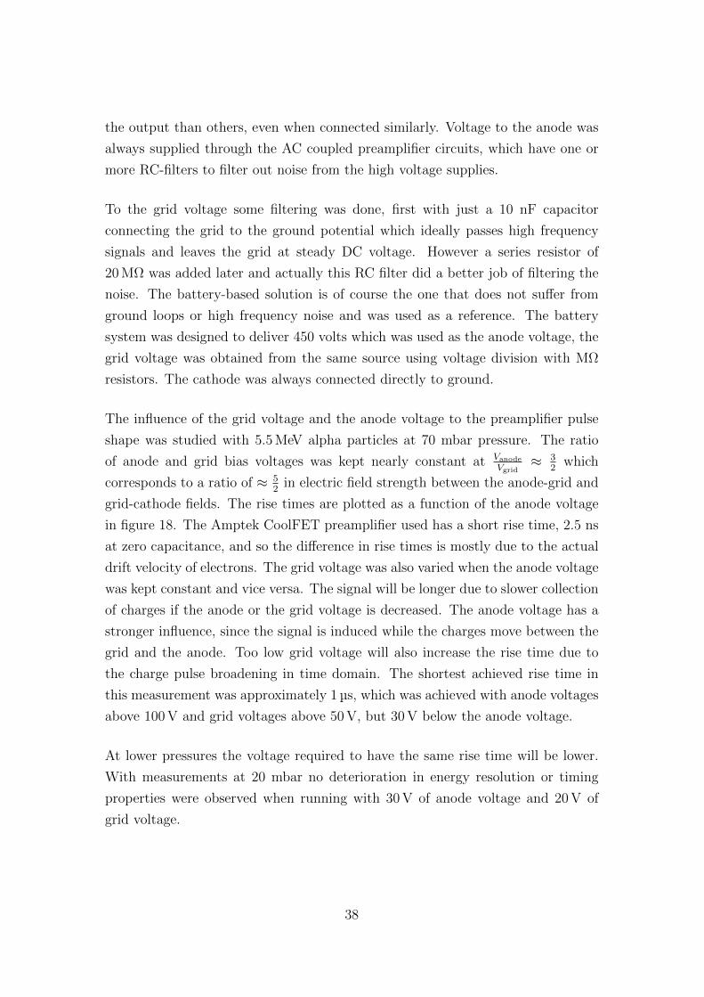
The influence of the grid voltage and the anode voltage to the preamplifier pulse
shape was studied with 5.5 MeV alpha particles at 70 mbar pressure. The ratio
of anode and grid bias voltages was kept nearly constant at VanodeVgrid
≈ 32
which
corresponds to a ratio of ≈ 52
in electric field strength between the anode-grid and
grid-cathode fields. The rise times are plotted as a function of the anode voltage
in figure 18. The Amptek CoolFET preamplifier used has a short rise time, 2.5 ns
at zero capacitance, and so the difference in rise times is mostly due to the actual
drift velocity of electrons. The grid voltage was also varied when the anode voltage
was kept constant and vice versa. The signal will be longer due to slower collection
of charges if the anode or the grid voltage is decreased. The anode voltage has a
stronger influence, since the signal is induced while the charges move between the
grid and the anode. Too low grid voltage will also increase the rise time due to
the charge pulse broadening in time domain. The shortest achieved rise time in
this measurement was approximately 1 µs, which was achieved with anode voltages
above 100 V and grid voltages above 50 V, but 30 V below the anode voltage.
At lower pressures the voltage required to have the same rise time will be lower.
With measurements at 20 mbar no deterioration in energy resolution or timing
properties were observed when running with 30 V of anode voltage and 20 V of
grid voltage.
38
0
1
2
3
4
5
6
7
8
9
0 20 40 60 80 100 120 140 160
Ris
eti
me (
µs)
Anode voltage (V)
Preamplifier pulse rise time
Figure 18: Rise time of preamplifier pulses as a function of anode voltage at 70mbar of pressure for 5.5 MeV alpha particles. The ratio of grid and anode biasvoltages was kept constant at Vanode
Vgrid≈ 3
2. The high voltage supply might have a
large unknown uncertainty in the voltage reading.
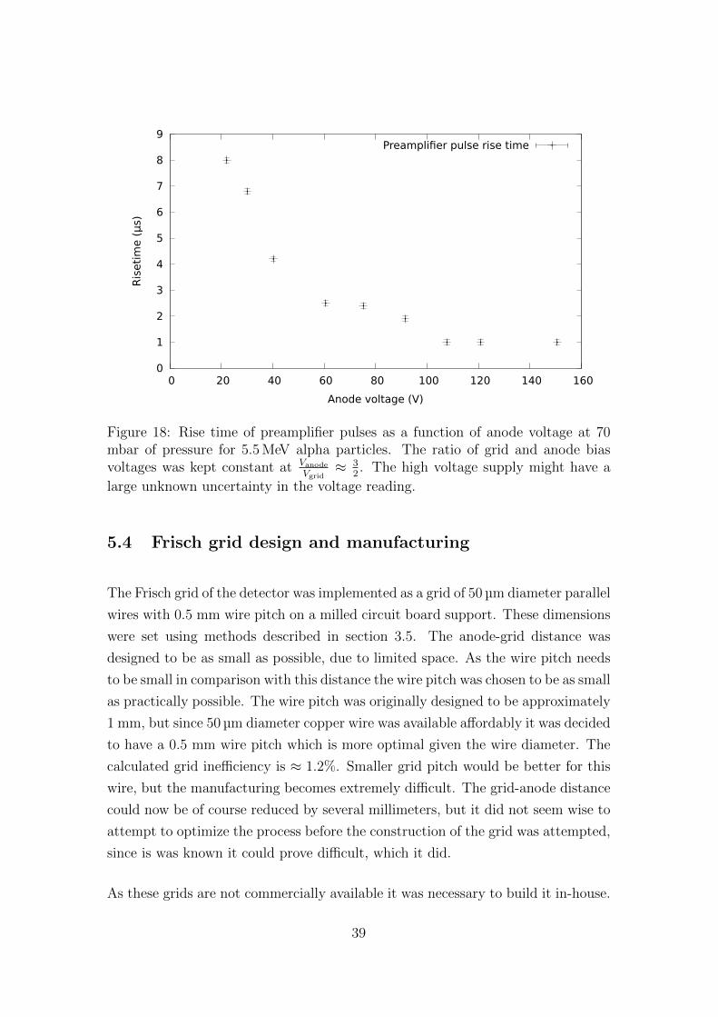
5.4 Frisch grid design and manufacturing
The Frisch grid of the detector was implemented as a grid of 50 µm diameter parallel
wires with 0.5 mm wire pitch on a milled circuit board support. These dimensions
were set using methods described in section 3.5. The anode-grid distance was
designed to be as small as possible, due to limited space. As the wire pitch needs
to be small in comparison with this distance the wire pitch was chosen to be as small
as practically possible. The wire pitch was originally designed to be approximately
1 mm, but since 50 µm diameter copper wire was available affordably it was decided
to have a 0.5 mm wire pitch which is more optimal given the wire diameter. The
calculated grid inefficiency is ≈ 1.2%. Smaller grid pitch would be better for this
wire, but the manufacturing becomes extremely difficult. The grid-anode distance
could now be of course reduced by several millimeters, but it did not seem wise to
attempt to optimize the process before the construction of the grid was attempted,
since is was known it could prove difficult, which it did.
As these grids are not commercially available it was necessary to build it in-house.
39

Wires were spun on top of a copperized circuit board using a custom made alu-
minium mount with the help of threaded rods. Wires were spun perpendicular
to the direction of detected particles. Copper wire was chosen as it was the most
economical and no issues were expected due to the wires being oxidised. Tung-
sten wires or gold plated tungsten wires are of course the best choice since they
have higher tensile strength. But already at 50 µm diameter even pure copper wire
proved to be adequately strong.
Threaded rods have a standard metric M3 thread, which means they have 0.5 mm
pitch and 3 mm outer diameter. Other wire pitches require different threads. The
process of spinning the wires will be more difficult with thinner rods, but threaded
rods are also available in finer pitches. Wires should excert enough force on the
circuit board to create a stable grid even under gravity and electrostatic forces [21].
The tension is limited by the supporting circuit board, material of the wires and
the process of making the grid.
The circuit board is carefully attached to the aluminium support. Any deforma-
tions in the circuit board are not welcome, since these have an effect on the pull
of individual wires and could result in some wires being loose.
After wires are spun they are glued on the circuit board using epoxy. It is critical
that wires are in good contact with the copper surface at this stage, otherwise
electrical contant between the wires and the circuit board could be compromised.
Easiest way to be sure the contact is good is to use conductive epoxy which is
commercially available or solder the wires in stead of gluing. Conductive epoxy
contains enough silver particles to conduct electricity but still retains most of the
mechanical properties of epoxy. After epoxy has dried wires can be cut.
This process however did not yield good grids since most of the wires were loose.
The 500 rounds of copper wire will always excert force on the circuit board un-
evenly. The tension of wires was improved by supporting the grid to the anode
using plastic blocks. These insulating blocks wrap around the anode and are at-
tached to the sides of the grid using instant glue or epoxy. The block is compressed
immediately after glue is applied, and held compressed until the glue has dried.
After compression is removed the plastic block relaxes and spreads the grid tight-
ening the wires. One block is enough to tighten wires in a few centimeters area, so
40

several are needed for this 250 mm long grid. A photograph of a grid manufactured
using this process is in figure 19.
Figure 19: Picture of a Frisch grid after tightening. The wires of 50 µm diameter ofthis grid are glued using regular epoxy at 0.5 mm intervals on a single sided PCB.The total anode length is 250 mm corresponding to 500 wires. The distance thewires hang unsupported is 40 mm. The insulating black plastic blocks increase thetension of the wires and attach the grid frame to the anode 8 mm below the wireplane.
Alternative process of manufacturing the grid was also attempted. In this process
wires are spun on threaded rods and a similar circuit board as previously is glued
to the spunned harp. This one-shot process would be slightly easier but in reality
yielded looser wires than the method described above.
5.5 Calibration and resolution
5.5.1 Energy calibration
Calibration measurements were initially done with scattered beam from thick sam-
ple containing one or more heavy elements, since we detect only a single nuclide,
namely the backscattered or forward scattered incident beam. There is no need to
41

separate different elements and measurements with heavy ions is simplified. These
measurements can be used to obtain an energy calibration since the scattered beam
has a known maximum energy when indicent beam energy, scattering angle and
heaviest sample element are known. This requires multiple measurements with
varying incident beam energy, since only one point of calibration is obtained for
each measurement.
It is much more convenient to calibrate the gas ionization detector against the
energy obtained with time of flight measurement. Now the full spectrum where
different masses can be separated can be used to perform calibration. A second
order polynomial fit for 12C is plotted in figure 20.
200
400
600
800
1000
1200
1400
1600
1800
200 400 600 800 1000 1200 1400 1600 1800 2000
GIC
cha
nnel
E from ToF (keV)
00831 12-CGIC calibration
Figure 20: The energy calibration of the GIC for 12C. The fitted polynomial isE = 152.3 keV + 1.172 keV/ch× channel− 9.981 · 10−5 keV/ch2 × channel2.
42

5.5.2 Energy resolution
To obtain resolution at some E we can choose events near E and calculate the dis-
tribution of EGIC
ETOF. If time-of-flight measurement is assumed to have better energy
resolution in comparison with the GIC measurement, which holds at least for heavy
recoils, the deviation from unity is mainly due to the limited resolution of the GIC.
The relative error can be then multiplied with E to obtain absolute resolution at
E. An example of distribution of values of EGIC
ETOFis in figure 21. In figure 22 the
resolution of the GIC is plotted for different elements at different energies. Since
the noise seems to have very little dependence on energy it is presumed the resolu-
tion is limited by electronics noise. This assumption is backed up by the obtained
25 keV resolution for hydrogen, since electronics noise with Ortec 142B preampli-
fier with W=26.3 eV/pair alone limits the resolution to 2.6 keV × 26.33.63≈ 19 keV.
0
5
10
15
20
25
30
35
0.9 0.95 1 1.05 1.1
Cou
nts
EGIC/ETOF
00831 1150-1250 keV 12-CGaussian fit
Figure 21: The distribution of calibrated values of EGIC
ETOFbetween 1150 keV and
1250 keV for 12C. The gaussian fit has a mean of 1.0001 and standard deviation of0.0152, which corresponds to a FWHM resolution of 43 keV at 1200 keV.
43
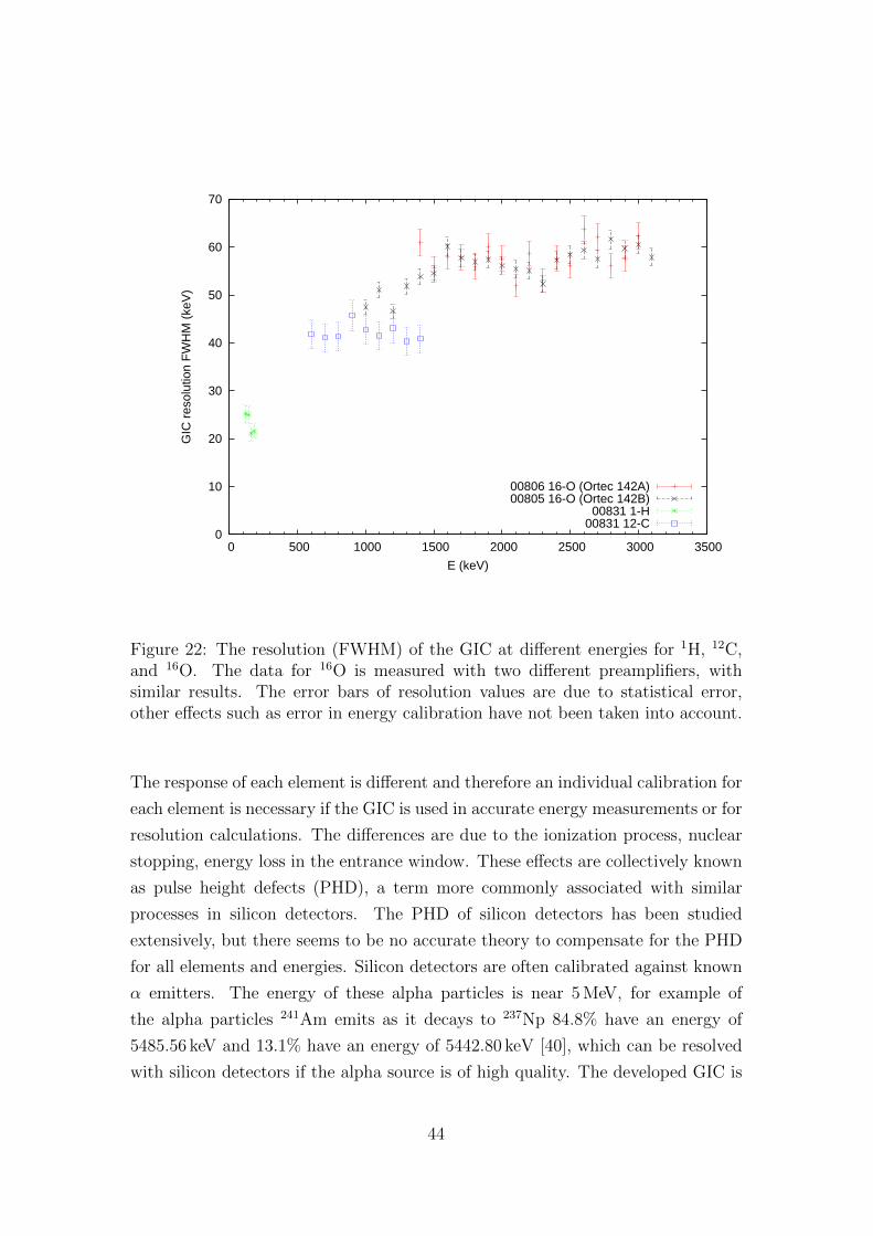
0
10
20
30
40
50
60
70
0 500 1000 1500 2000 2500 3000 3500
GIC
res
olut
ion
FW
HM
(ke
V)
E (keV)
00806 16-O (Ortec 142A)00805 16-O (Ortec 142B)
00831 1-H00831 12-C
Figure 22: The resolution (FWHM) of the GIC at different energies for 1H, 12C,and 16O. The data for 16O is measured with two different preamplifiers, withsimilar results. The error bars of resolution values are due to statistical error,other effects such as error in energy calibration have not been taken into account.
The response of each element is different and therefore an individual calibration for
each element is necessary if the GIC is used in accurate energy measurements or for
resolution calculations. The differences are due to the ionization process, nuclear
stopping, energy loss in the entrance window. These effects are collectively known
as pulse height defects (PHD), a term more commonly associated with similar
processes in silicon detectors. The PHD of silicon detectors has been studied
extensively, but there seems to be no accurate theory to compensate for the PHD
for all elements and energies. Silicon detectors are often calibrated against known
α emitters. The energy of these alpha particles is near 5 MeV, for example of
the alpha particles 241Am emits as it decays to 237Np 84.8% have an energy of
5485.56 keV and 13.1% have an energy of 5442.80 keV [40], which can be resolved
with silicon detectors if the alpha source is of high quality. The developed GIC is
44
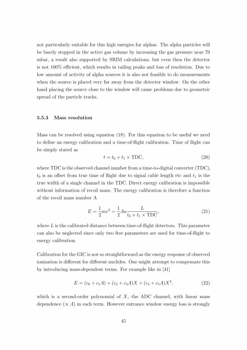
not particularly suitable for this high energies for alphas. The alpha particles will
be barely stopped in the active gas volume by increasing the gas pressure near 70
mbar, a result also supported by SRIM calculations, but even then the detector
is not 100% efficient, which results in tailing peaks and loss of resolution. Due to
low amount of activity of alpha sources it is also not feasible to do measurements
when the source is placed very far away from the detector window. On the other
hand placing the source close to the window will cause problems due to geometric
spread of the particle tracks.
5.5.3 Mass resolution
Mass can be resolved using equation (18). For this equation to be useful we need
to define an energy calibration and a time-of-flight calibration. Time of flight can
be simply stated as
t = t0 + t1 × TDC, (20)
where TDC is the observed channel number from a time-to-digital converter (TDC),
t0 is an offset from true time of flight due to signal cable length etc and t1 is the
true width of a single channel in the TDC. Direct energy calibration is impossible
without information of recoil mass. The energy calibration is therefore a function
of the recoil mass number A
E =1
2mv2 =
1
2Au
L
t0 + t1 × TDC, (21)
where L is the calibrated distance between time-of-flight detectors. This parameter
can also be neglected since only two free parameters are used for time-of-flight to
energy calibration.
Calibration for the GIC is not so straightforward as the energy response of observed
ionization is different for different nuclides. One might attempt to compensate this
by introducing mass-dependent terms. For example like in [41]
E = (c0 + c1A) + (c2 + c3A)X + (c4 + c5A)X2, (22)
which is a second-order polynomial of X, the ADC channel, with linear mass
dependence (∝ A) in each term. However entrance window energy loss is strongly
45
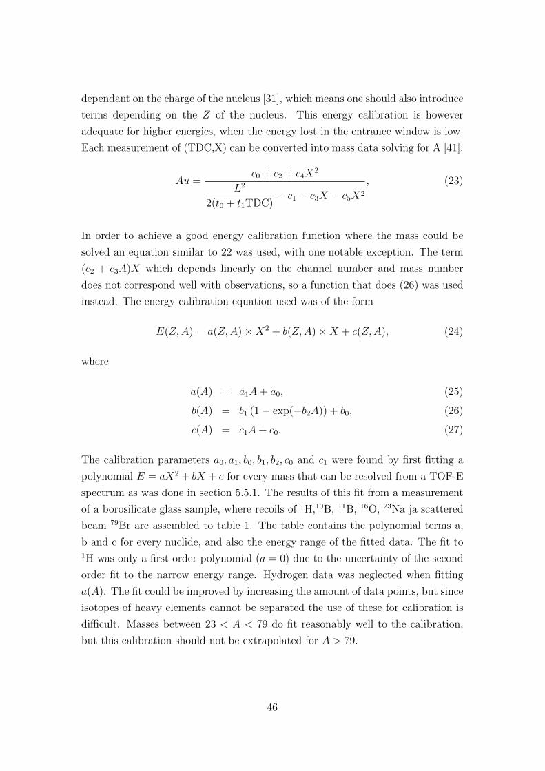
dependant on the charge of the nucleus [31], which means one should also introduce
terms depending on the Z of the nucleus. This energy calibration is however
adequate for higher energies, when the energy lost in the entrance window is low.
Each measurement of (TDC,X) can be converted into mass data solving for A [41]:
Au =c0 + c2 + c4X
2
L2
2(t0 + t1TDC)− c1 − c3X − c5X2
, (23)
In order to achieve a good energy calibration function where the mass could be
solved an equation similar to 22 was used, with one notable exception. The term
(c2 + c3A)X which depends linearly on the channel number and mass number
does not correspond well with observations, so a function that does (26) was used
instead. The energy calibration equation used was of the form
E(Z,A) = a(Z,A)×X2 + b(Z,A)×X + c(Z,A), (24)
where
a(A) = a1A+ a0, (25)
b(A) = b1 (1− exp(−b2A)) + b0, (26)
c(A) = c1A+ c0. (27)
The calibration parameters a0, a1, b0, b1, b2, c0 and c1 were found by first fitting a
polynomial E = aX2 + bX + c for every mass that can be resolved from a TOF-E
spectrum as was done in section 5.5.1. The results of this fit from a measurement
of a borosilicate glass sample, where recoils of 1H,10B, 11B, 16O, 23Na ja scattered
beam 79Br are assembled to table 1. The table contains the polynomial terms a,
b and c for every nuclide, and also the energy range of the fitted data. The fit to1H was only a first order polynomial (a = 0) due to the uncertainty of the second
order fit to the narrow energy range. Hydrogen data was neglected when fitting
a(A). The fit could be improved by increasing the amount of data points, but since
isotopes of heavy elements cannot be separated the use of these for calibration is
difficult. Masses between 23 < A < 79 do fit reasonably well to the calibration,
but this calibration should not be extrapolated for A > 79.
46
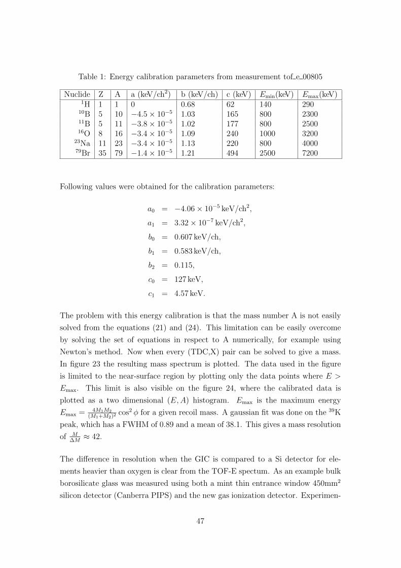
Table 1: Energy calibration parameters from measurement tof e 00805
Nuclide Z A a (keV/ch2) b (keV/ch) c (keV) Emin(keV) Emax(keV)1H 1 1 0 0.68 62 140 290
10B 5 10 −4.5× 10⁻⁵ 1.03 165 800 230011B 5 11 −3.8× 10⁻⁵ 1.02 177 800 250016O 8 16 −3.4× 10⁻⁵ 1.09 240 1000 3200
23Na 11 23 −3.4× 10⁻⁵ 1.13 220 800 400079Br 35 79 −1.4× 10⁻⁵ 1.21 494 2500 7200
Following values were obtained for the calibration parameters:
a0 = −4.06× 10⁻⁵ keV/ch2,
a1 = 3.32× 10⁻⁷ keV/ch2,
b0 = 0.607 keV/ch,
b1 = 0.583 keV/ch,
b2 = 0.115,
c0 = 127 keV,
c1 = 4.57 keV.
The problem with this energy calibration is that the mass number A is not easily
solved from the equations (21) and (24). This limitation can be easily overcome
by solving the set of equations in respect to A numerically, for example using
Newton’s method. Now when every (TDC,X) pair can be solved to give a mass.
In figure 23 the resulting mass spectrum is plotted. The data used in the figure
is limited to the near-surface region by plotting only the data points where E >
Emax. This limit is also visible on the figure 24, where the calibrated data is
plotted as a two dimensional (E,A) histogram. Emax is the maximum energy
Emax = 4M1M2
(M1+M2)2cos2 φ for a given recoil mass. A gaussian fit was done on the 39K
peak, which has a FWHM of 0.89 and a mean of 38.1. This gives a mass resolution
of M∆M≈ 42.
The difference in resolution when the GIC is compared to a Si detector for ele-
ments heavier than oxygen is clear from the TOF-E spectum. As an example bulk
borosilicate glass was measured using both a mint thin entrance window 450mm2
silicon detector (Canberra PIPS) and the new gas ionization detector. Experimen-
47

Cou
nts
Mass (amu)
00805Gaussian fit to K−39
1
10
100
1000
0 10 20 30 40 50 60 70 80
Si−28
Si−29Si−30
B−10
B−11
O−16
Na−23K−39
K−41
H−1
Ti−46,47,48,49,50Br−79
Zn−64,66,67,68
Fe−56?
Figure 23: Mass spectrum of a borosilicate glass sample determined from the time-of-flight–energy measurement. A gaussian fit was done on the 39K peak.
tal setup was identical with 10.2 MeV 79Br beam. The larger solid angle of the
silicon detector does not affect mass resolution. From figure 25 one can see how
the ionization detector outperforms Si detector even for 10B although the resolu-
tion of the GIC could still be improved by a factor of two by reducing electronics
noise. For heavier recoils and lower energies the difference in resolution is even
more pronounced.
48
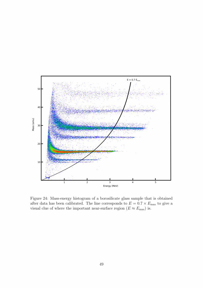
Figure 24: Mass-energy histogram of a borosilicate glass sample that is obtainedafter data has been calibrated. The line corresponds to E = 0.7× Emax to give avisual clue of where the important near-surface region (E ≈ Emax) is.
49
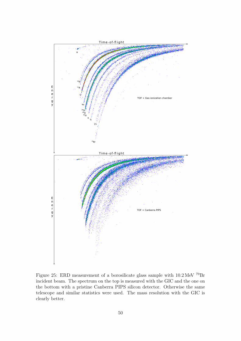
Figure 25: ERD measurement of a borosilicate glass sample with 10.2 MeV 79Brincident beam. The spectrum on the top is measured with the GIC and the one onthe bottom with a pristine Canberra PIPS silicon detector. Otherwise the sametelescope and similar statistics were used. The mass resolution with the GIC isclearly better.
50

5.5.4 Position resolution
Position sensitivity is demonstrated in figure 26. This measurement was performed
with 5.5 MeV alpha particles emitted by 241Am source and a collimator with three
1 mm wide slits 3 mm apart from each other. The cathode signal was also acquired
in the ERD measurements done with the detector. The 5 mm wide window was not
large enough to clearly demonstrate position sensitivity with the obtained energy or
cathode resolution. The cathode signals were successfully acquired in coincidence
with the anode signal and a linear dependence between them was observed. Had
the position resolution been a major focus a collimator should have been placed
before the window, but this was prevented due to lack of measurement time and
larger windows.
Figure 26: Position sensitivity demonstrated with a collimator near entrance win-dow for 5.5 MeV alphas from Am-241 source. Energy resolution of the detectorwas further improved after these measurements. The position axis is simply cath-ode ADC signal divided by the anode ADC signal (energy) without any correction.Brighter colors stand for higher intensity in the 2D histogram. The projected 1Dposition histogram is also plotted.
51

5.6 Data aqcuisition and coincidence processing
In TOF-E measurements data was acquired by means of a National Instruments
FPGA data acquisition system which reads time-of-flight from a FAST ComTec
7072T TDC (ADC0) and energy signal from another channel of the same device
operating as an ADC (ADC1). The TDC/ADC has a 500 ns fixed conversion time
13-bit ADC. Additionally cathode signal was acquired from another ADC (ADC2).
There is no triggering between ADC0, ADC1 or ADC2 events, but the events are
timestamped with 25 ns precision by the FPGA, which corresponds to one clock
tick at 40 MHz.
A piece of software was written to do the offline coincidence processing. The
program works by attempting to find the closest ADC1 (E) event to every ADC0
(TOF) event inside a given time window. The program can find false coincidences
but does not lose any real coincidences, since there cannot be two energy counts
inside the same timing window due to the TDC conversion time of 500 ns and ADC
dead time between 1 and 3 µs if the spectroscopy amplifier has pile-up rejection.
Coincidences are processed so that all ADC0 events within the timing window for
a given ADC1 event are found.
In figure 27 a histogram of timestamp differences is plotted with a gaussian fit. It
can be seen that most of the 114000 counts fall inside the bell curve which has
an area corresponding to 105000 counts. Most of the counts outside the gaussian
fit come from the fact that the timing accuracy of the energy detector is energy
dependant. The timing is done between the TDC and ADC events. Spectroscopy
amplifier output pulse does have predictable rise time from zero level to maximum
assuming there is no pile-up and the ADC conversion starts some time after the
maximum. Low frequency noise in the spectroscopy amplifier output will cause
timing jitter by delaying or advancing the start of conversion. This error is larger
for small pulse heights due to the gaussian shape and therefore also proportional to
the shaping time. In figure 28 an intensity map of ADC1 values versus timestamp
difference to ADC0 are plotted.
By choosing a tight window we can eliminate some of the false coincidences but
choosing too tight a window can result in unwanted statistical bias. In ERD mea-
surements the low energy end is important due to small signals from hydrogen.
52

Coincidence window could also be set so that it is wider for the TOF range where
hydrogen signal is observed. Improvement in the background noise elimination re-
quires good timing properties and short pulses from the detector. In this situation
thin silicon detectors – particularly those which have improved timing properties –
outperform gas ionization detector. The timing accuracy can also be improved by
employing digital pulse processing instead of the conventional analog electronics
chain.
Cou
nts
Timestamp difference (25 ns ticks)
Timestamp difference of ADC0 and ADC1Gaussian fit
1
10
100
1000
10000
140 160 180 200 220 240 260 280 300 320 340
Figure 27: Timestamp difference between ADC0 (time-of-flight) and ADC1 (en-ergy). The timing window used for this measurement is marked with vertical linesat ticks 226 and 262. There is a nearly constant background outside the peak. Agaussian fit is attempted on the peak, the mean is 244.7 ticks, standard deviation2.1 ticks and area 105000 counts. There are a total of 114492 counts plotted be-tween 140 and 340 ticks. The inset shows the same peak from ticks 226 to 262 ona linear vertical scale.
53
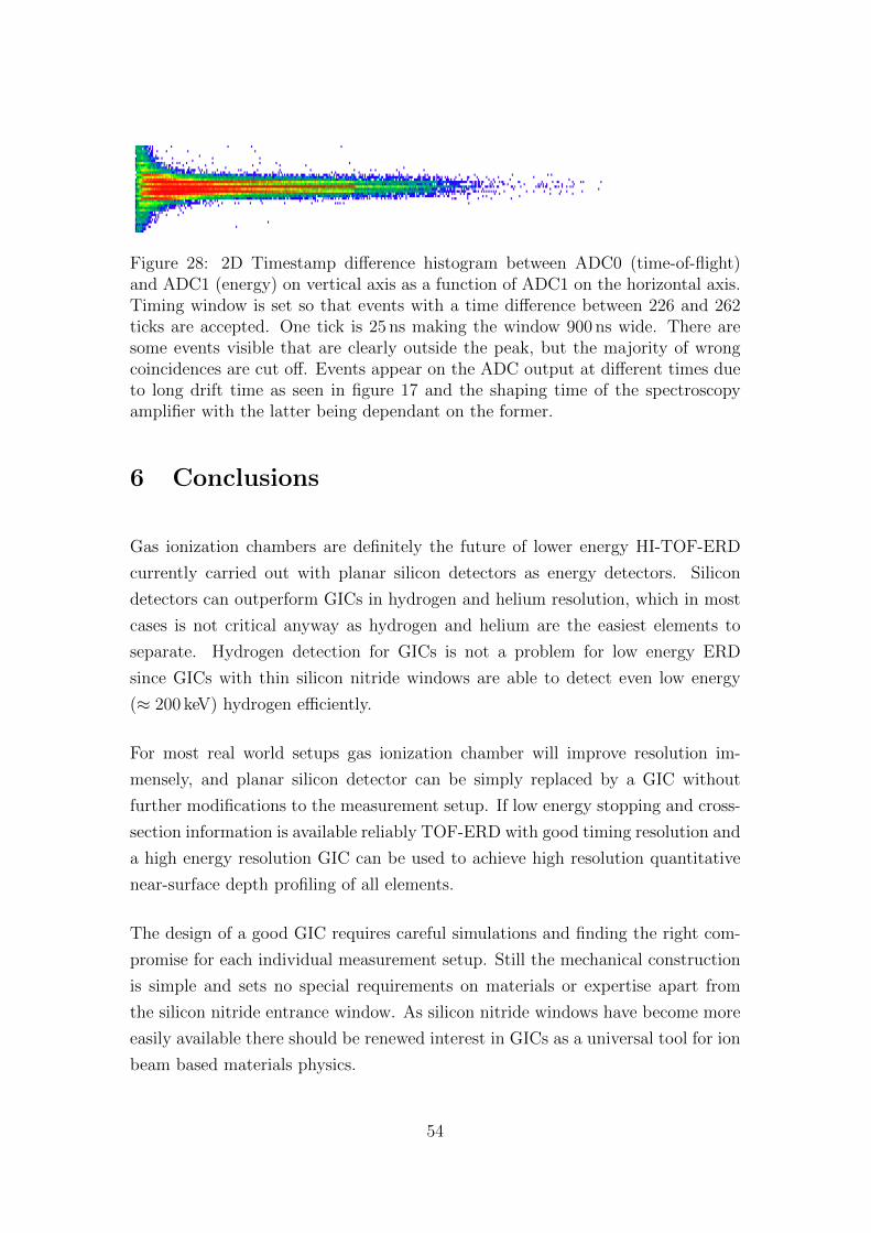
Figure 28: 2D Timestamp difference histogram between ADC0 (time-of-flight)and ADC1 (energy) on vertical axis as a function of ADC1 on the horizontal axis.Timing window is set so that events with a time difference between 226 and 262ticks are accepted. One tick is 25 ns making the window 900 ns wide. There aresome events visible that are clearly outside the peak, but the majority of wrongcoincidences are cut off. Events appear on the ADC output at different times dueto long drift time as seen in figure 17 and the shaping time of the spectroscopyamplifier with the latter being dependant on the former.
6 Conclusions
Gas ionization chambers are definitely the future of lower energy HI-TOF-ERD
currently carried out with planar silicon detectors as energy detectors. Silicon
detectors can outperform GICs in hydrogen and helium resolution, which in most
cases is not critical anyway as hydrogen and helium are the easiest elements to
separate. Hydrogen detection for GICs is not a problem for low energy ERD
since GICs with thin silicon nitride windows are able to detect even low energy
(≈ 200 keV) hydrogen efficiently.
For most real world setups gas ionization chamber will improve resolution im-
mensely, and planar silicon detector can be simply replaced by a GIC without
further modifications to the measurement setup. If low energy stopping and cross-
section information is available reliably TOF-ERD with good timing resolution and
a high energy resolution GIC can be used to achieve high resolution quantitative
near-surface depth profiling of all elements.
The design of a good GIC requires careful simulations and finding the right com-
promise for each individual measurement setup. Still the mechanical construction
is simple and sets no special requirements on materials or expertise apart from
the silicon nitride entrance window. As silicon nitride windows have become more
easily available there should be renewed interest in GICs as a universal tool for ion
beam based materials physics.
54

7 References
[1] J. L’Ecuyer, C. Brassard, C. Cardinal, J. Chabbal, L. Deschenes, J. P. Labrie,
B. Terreault, J. G. Martel, and R. St.-Jacques. An accurate and sensitive
method for the determination of the depth distribution of light elements in
heavy materials. Journal of Applied Physics, 47(1):381–382, 1976.
[2] W. Bohne, J. Rohrich, and G. Roschert. The new time-of-flight ERDA setup
at the HMI-Berlin. Nuclear Instruments and Methods in Physics Research
Section B: Beam Interactions with Materials and Atoms, 139(1-4):219 – 224,
1998.
[3] W. Assmann, P. Hartung, H. Huber, P. Staat, H. Steffens, and Ch. Stein-
hausen. Setup for materials analysis with heavy ion beams at the Munich MP
tandem. Nuclear Instruments and Methods in Physics Research Section B:
Beam Interactions with Materials and Atoms, 85(1-4):726 – 731, 1994.
[4] H. Timmers, R. G. Elliman, G. R. Palmer, T. R. Ophel, and D. J. O’Connor.
The development of a facility for heavy-ion elastic recoil detection analysis
at the Australian National University. Nuclear Instruments and Methods in
Physics Research Section B: Beam Interactions with Materials and Atoms,
136-138:611 – 615, 1998. Ion Beam Analysis.
[5] R. Groleau, S.C. Gujrathi, and J.P. Martin. Time-of-flight system for profiling
recoiled light elements. Nuclear Instruments and Methods in Physics Research,
218(1-3):11 – 15, 1983.
[6] C.R. Gossett. Use of a magnetic spectrometer to profile light elements by
elastic recoil detection. Nuclear Instruments and Methods in Physics Research
Section B: Beam Interactions with Materials and Atoms, 15(1-6):481 – 485,
1986.
[7] G. Dollinger, M. Boulouednine, T. Faestermann, and P. Maier-Komor. Depth
microscopy for thin film analysis. Nuclear Instruments and Methods in Physics
Research Section A: Accelerators, Spectrometers, Detectors and Associated
Equipment, 334(1):187 – 190, 1993.
55

[8] W. Assmann. Ionization chambers for materials analysis with heavy ion
beams. Nuclear Instruments and Methods in Physics Research Section B:
Beam Interactions with Materials and Atoms, 64(1-4):267 – 271, 1992.
[9] G. Pausch, W. Bohne, and D. Hilscher. Particle identification in solid-state
detectors by means of pulse-shape analysis – results of computer simulations.
Nuclear Instruments and Methods in Physics Research Section A: Accelera-
tors, Spectrometers, Detectors and Associated Equipment, 337(2-3):573 – 587,
1994.
[10] S. Giangrandi, T. Sajavaara, B. Brijs, K. Arstila, A. Vantomme, and W. Van-
dervorst. Low-energy heavy-ion TOF-ERDA setup for quantitative depth
profiling of thin films. Nuclear Instruments and Methods in Physics Research
Section B: Beam Interactions with Materials and Atoms, 266(24):5144 – 5150,
2008.
[11] C. Kottler, M. Dobeli, F. Glaus, and M. Suter. A spectrometer for low energy
heavy ion ERDA. Nuclear Instruments and Methods in Physics Research
Section B: Beam Interactions with Materials and Atoms, 248(1):155 – 162,
2006.
[12] M. Laitinen, T. Sajavaara, M. Rossi, J. Julin, R.L. Puurunen, T. Suni,
T. Ishida, H. Fujita, K. Arstila, B. Brijs, and H.J. Whitlow. Depth profiling of
Al2O3+TiO2 nanolaminates by means of a time-of-flight energy spectrometer.
Nuclear Instruments and Methods in Physics Research Section B: Beam In-
teractions with Materials and Atoms, In Press, Accepted Manuscript:–, 2011.
[13] J. R. Tesmer and M. Nastasi. The Handbook of Modern Ion Beam Materials
Analysis. Materials Research Society, 1995.
[14] H. Bethe. Bremsformel fur elektronen relativistischer geschwindigkeit.
Zeitschrift fur Physik, 76:293–299, 1932.
[15] F. Bloch. Bremsvermogen von atomen mit mehreren elektronen. Zeitschrift
fur Physik, 81:363–376, 1933.
[16] J. Ziegler. The Stopping and Range of Ions in Matter (SRIM). http://www.
srim.org/.
[17] J. S. Lilley. Nuclear Physics: Principles and Applications. John Wiley &
Sons, New York, 2001.
56
[18] W. K. Chu. Calculation of energy straggling for protons and helium ions.
Phys. Rev. A, 13(6):2057–2060, Jun 1976.
[19] Q. Yang, D.J. O’Connor, and Zhonglie Wang. Empirical formulae for energy
loss straggling of ions in matter. Nuclear Instruments and Methods in Physics
Research Section B: Beam Interactions with Materials and Atoms, 61(2):149
– 155, 1991.
[20] G. F. Knoll. Radiation Detection and Measurement. John Wiley & Sons, New
York, 3rd edition, 2000.
[21] K. Kleinknecht. Detectors for Particle Radiation. Cambridge University Press,
second edition, 1998.
[22] U. Fano. Ionization yield of radiations. II. The fluctuations of the number of
ions. Phys. Rev., 72(1):26–29, 1947.
[23] Martin Suter, Max Dobeli, Michal Grajcar, Arnold Muller, Martin Stocker,
Guoyan Sun, Hans-Arno Synal, and Lukas Wacker. Advances in particle
identification in AMS at low energies. Nuclear Instruments and Methods in
Physics Research Section B: Beam Interactions with Materials and Atoms,
259(1):165 – 172, 2007. Accelerator Mass Spectrometry - Proceedings of the
Tenth International Conference on Accelerator Mass Spectrometry.
[24] B. Rossi and H. Staub. Ionization Chambers and Counters. McGraw-Hill
Book Company, Inc., first edition, 1949.
[25] W. Shockley. Currents to conductors induced by a moving point charge.
Journal of Applied Physics, 9, 1938.
[26] O. Frisch. Isotope analysis of uranium samples by means of their α-ray groups.
British Atomic Energy Project Report BR-49, 1944. Unpublished.
[27] P. S. Barbeau, J. I. Collar, J. D. Geissinger, J. Miyamoto, I. Shipsey, and
R. Yang. A first mass production of gas electron multipliers. Nuclear Instru-
ments and Methods in Physics Research Section A: Accelerators, Spectrome-
ters, Detectors and Associated Equipment, 515(3):439 – 445, 2003.
[28] M. Mallepell, M. Dobeli, and M. Suter. Annular gas ionization detector for
low energy heavy ion backscattering spectrometry. Nuclear Instruments and
57
Methods in Physics Research Section B: Beam Interactions with Materials and
Atoms, 267(7):1193 – 1198, 2009.
[29] A.M. Muller, A. Cassimi, M. Dobeli, M. Mallepell, I. Monnet, M.J. Simon,
M. Suter, and H.-A. Synal. A new mini gas ionization chamber for IBA
applications. Nuclear Instruments and Methods in Physics Research Sec-
tion B: Beam Interactions with Materials and Atoms, In Press, Accepted
Manuscript:–, 2011.
[30] M. Dobeli, C. Kottler, M. Stocker, S. Weinmann, H. A. Synal, M. Graj-
car, and M. Suter. Gas ionization chambers with silicon nitride windows for
the detection and identification of low energy ions. Nuclear Instruments and
Methods in Physics Research Section B: Beam Interactions with Materials and
Atoms, 219-220:415 – 419, 2004. Proceedings of the Sixteenth International
Conference on Ion Beam Analysis.
[31] G. Sun, M. Dobeli, A.M. Muller, M. Stocker, M. Suter, and L. Wacker. Energy
loss and straggling of heavy ions in silicon nitride in the low MeV energy
range. Nuclear Instruments and Methods in Physics Research Section B: Beam
Interactions with Materials and Atoms, 256(2):586 – 590, 2007.
[32] Silson Ltd. http://www.silson.com/.
[33] V. A. Khriachkov, A. A. Goverdovski, V. V. Ketlerov, V. F. Mitrofanov, and
N. N. Semenova. Direct experimental determination of frisch grid inefficiency
in ionization chamber. Nuclear Instruments and Methods in Physics Research
Section A: Accelerators, Spectrometers, Detectors and Associated Equipment,
394(1-2):261 – 264, 1997.
[34] O. Bunemann, T.E. Cranshaw, and J. A. Harvey. Design of Grid Ionization
Chambers. Canadian Journal of Research, 27, 1949.
[35] SIMION 8. http://www.simion.com/.
[36] D. Green. The Physics of Particle Detectors. Cambridge University Press,
2000.
[37] O. Forstner, L. Michlmayr, M. Auer, R. Golser, W. Kutschera, A. Priller,
P. Steier, and A. Wallner. Applications of a compact ionization chamber in
AMS at energies below 1 MeV/amu. Nuclear Instruments and Methods in
58
Physics Research Section B: Beam Interactions with Materials and Atoms,
266(10):2213 – 2216, 2008. Accelerators in Applied Research and Technology
- Proceedings of the 9th European Conference on Accelerators in Applied Re-
search and Technology, 9th European Conference on Accelerators in Applied
Research and Technology.
[38] H. Timmers, T. R. Ophel, and R. G. Elliman. Simplifying position-sensitive
gas-ionization detectors for heavy ion elastic recoil detection. Nuclear Instru-
ments and Methods in Physics Research Section B: Beam Interactions with
Materials and Atoms, 161-163:19 – 28, 2000.
[39] A. Gopfert, F. J. Hambsch, and H. Bax. A twin ionization chamber setup as
detector for light charged particles with energies around 1 MeV applied to the10B(n, α)7Li reaction. Nuclear Instruments and Methods in Physics Research
Section A: Accelerators, Spectrometers, Detectors and Associated Equipment,
441(3):438 – 451, 2000.
[40] M.S. Basunia. Nuclear Data Sheets for A = 237. Nuclear Data Sheets,
107(8):2323 – 2422, 2006.
[41] M. E. Bouanani, M. Hult, L. Persson, E. Swietlicki, M. Andersson, M. Ostling,
N. Lundberg, C. Zaring, D. D. Cohen, N. Dytlewski, P. N. Johnston, S. R.
Walker, I. F. Bubb, and H. J. Whitlow. Multivariate analysis method for en-
ergy calibration and improved mass assignment in recoil spectrometry. Nuclear
Instruments and Methods in Physics Research Section B: Beam Interactions
with Materials and Atoms, 94(4):530 – 536, 1994.
59


![Ionization chambers Proportional counters Geiger Muller counterssleoni/TEACHING/Nuc-Phys-Det/PDF/... · 2014-10-21 · Gas Detectors [the oldest detectors] ! Ionization chambers !](https://static.fdocuments.net/doc/165x107/5eb629c512a9904888072f04/ionization-chambers-proportional-counters-geiger-muller-sleoniteachingnuc-phys-detpdf.jpg)