Development of a Continuous Blending System1 - … document/5282_full...Development of a Continuous...

Ind

ust

rial E

lectr

ical En

gin

eerin

g a

nd

A

uto

matio

n

CODEN:LUTEDX/(TEIE-5282)/1-59(2011)

Development of a ContinuousBlending System

Eli Al Hadawi

Division of Industrial Electrical Engineering and Automation Faculty of Engineering, Lund University

M.Sc. Thesis within Electrical Engineering, 30 points

Development of a Continuous Blending System

Controlling a blending system

Eli Al Hadawi

Lund University Faculty of Engineering Division of Industrial Electrical Engineering and Automation (IEA) Author: Eli Al Hadawi E-mail address: [email protected] Study programme: Master of Science, EE, 300 p Examiner: Dr. Ulf Jeppsson, [email protected] Supervisor: Dr. Gunnar Lindstedt, [email protected] Scope: 7519 words Date: 2011-03-24

Eli Al Hadawi

Abstract

2011‐06‐07

ii

Abstract The company QB Food Tech designs and installs powder in liquid

mixing systems for the food and pharmaceutical industries. The aim of

this master thesis is to develop a continuous blending system with

concentration output feedback for inline blending of complex products

starting from an existing batch process. A method for measuring a

substance concentration in flow‐rates therefore needs to be established.

The measured concentration signal is then used for controlling the

inflow rate of raw materials; a PID controller block is used for achieving

this task. The whole system is PLC controlled and programmed in

Siemens SIMATIC STEP7 software. An HMI operator‐panel enables

parameter adjustments and results of the monitored concentration and

relevant actuators are shown in real‐time via the panel.

Keywords: PLC, HMI, STEP7, Inline blending, PID.

Development of a Continuous

Blending System Table of Contents

2011‐06‐07

iii

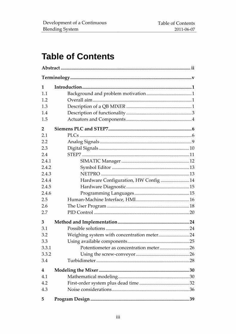
Table of Contents Abstract ............................................................................................................. ii

Terminology......................................................................................................v

1 Introduction............................................................................................1

1.1 Background and problem motivation ......................................1

1.2 Overall aim...................................................................................1

1.3 Description of a QB MIXER .......................................................1

1.4 Description of functionality .......................................................3

1.5 Actuators and Components .......................................................4

2 Siemens PLC and STEP7......................................................................6

2.1 PLCs ..............................................................................................6

2.2 Analog Signals .............................................................................9

2.3 Digital Signals ............................................................................10

2.4 STEP7 ..........................................................................................11

2.4.1 SIMATIC Manager .........................................................12

2.4.2 Symbol Editor .................................................................13

2.4.3 NETPRO ..........................................................................13

2.4.4 Hardware Configuration, HW Config ........................14

2.4.5 Hardware Diagnostic.....................................................15

2.4.6 Programming Languages..............................................15

2.5 Human‐Machine Interface, HMI.............................................16

2.6 The User Program .....................................................................18

2.7 PID Control ................................................................................20

3 Method and Implementation............................................................24

3.1 Possible solutions ......................................................................24

3.2 Weighing system with concentration meter..........................24

3.3 Using available components....................................................25

3.3.1 Potentiometer as concentration meter.........................26

3.3.2 Using the screw‐conveyor.............................................26

3.4 Turbidimeter ..............................................................................28

4 Modeling the Mixer ............................................................................30

4.1 Mathematical modeling............................................................30

4.2 First‐order system plus dead time ..........................................32

4.3 Noise considerations.................................................................36

5 Program Design ...................................................................................39


Blending System Table of Contents

2011‐06‐07

iv

5.1 Time representation ..................................................................39

5.2 Scaling .........................................................................................41

5.3 State machine .............................................................................42

5.3.1 The program controller FB33........................................42

5.3.2 Initial dosing FB34..........................................................44

5.3.3 Concentration PID FB35 ................................................45

5.4 Interrupt routine OB35 .............................................................46

5.5 HMI .............................................................................................46

5.6 Running the program ...............................................................48

6 Conclusions ..........................................................................................50

7 Further Development .........................................................................51

References........................................................................................................52


Blending System Terminology

2011‐06‐07

v

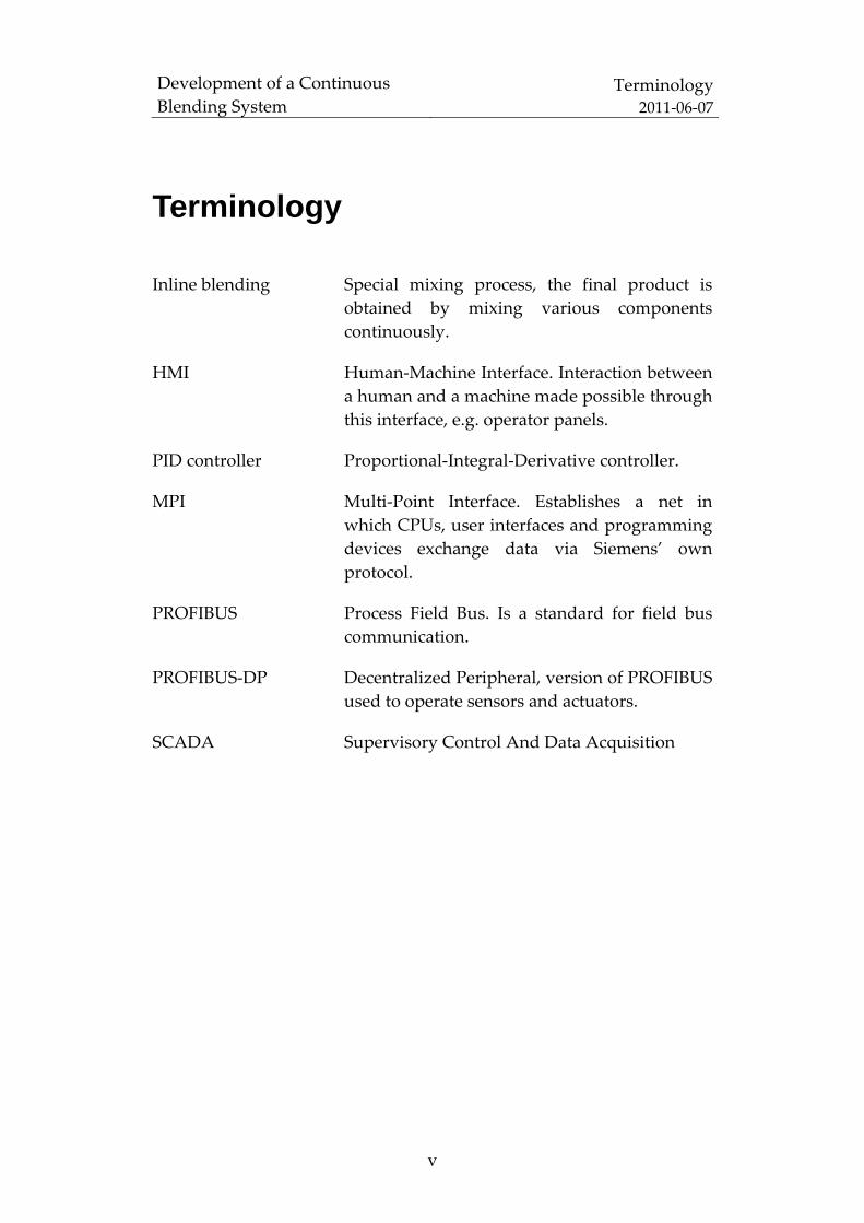
Terminology

Inline blending Special mixing process, the final product is

obtained by mixing various components

continuously.

HMI Human‐Machine Interface. Interaction between

a human and a machine made possible through

this interface, e.g. operator panels.

PID controller Proportional‐Integral‐Derivative controller.

MPI Multi‐Point Interface. Establishes a net in

which CPUs, user interfaces and programming

devices exchange data via Siemens’ own

protocol.

PROFIBUS Process Field Bus. Is a standard for field bus

communication.

PROFIBUS‐DP Decentralized Peripheral, version of PROFIBUS

used to operate sensors and actuators.

SCADA Supervisory Control And Data Acquisition


Blending System Introduction

2011‐06‐07

1

1 Introduction The chapter presents a background of the project and a short description

of the available mixer, its main actuators and sensors.

1.1 Background and problem motivation The market demands on the dairy, food and pharmaceutical industries

to produce a wide range of products led manufacturers to run more

batches to handle this diversity of flavours and mixed products. Batch

processes are therefore often converted to continuous ones. Mixing

plays a crucial role in the whole production process. A fast continuous

mixer with just‐in‐time mixing capability can easily be integrated in a

continuous production line and reduce the number of buffer storage

tanks.

The company QB Food Tech manufactures three different variants of the

QB MIXER meeting the different needs demanded by the market. Two

of these mixers are fully developed. This Master thesis will bring to light

the third QB MIXER being the continuous mixer in the QB MIXER

family. The new mixer equipped with extra sensors providing feedback

of the outflow concentration to the PLC Programmable Logic Controller

thus ensuring a better and more exact concentration control by

manipulating the relevant system actuators.

1.2 Overall aim The projectʹs overall aim is to develop a fully automated real time

blending system starting from an existing non‐continuous batch system.

The new system should guarantee a specific desired concentration of the

solid substance in the solvent making the final mixed product. It is also

intended to test the new system with a range of products to verify the

desired functionality.

1.3 Description of a QB MIXER The QB MIXER is primarily intended for mixing powder in liquid. It is a

production machine controlled by a single PLC. A sketch overview is

depicted in Figure 1.



2011‐06‐07

2

Figure 1: QB Mixer [1].

The principle of mixing creating the characteristic effective flow pattern

thanks to the cubical shape of the QB MIXER is depicted in Figure 2.

Figure 2: Flow pattern inside the tank [1].

The flow pattern keeps the vortex to a minimum yielding an effective

mixing. Batch sizes can vary from 30 to 4000 litres with output streams

up to 50.000 litres/hour.



2011‐06‐07

3

1.4 Description of functionality A signal from the operator HMI Human‐machine Interface touch panel

starts the filling of the solvent (usually water or milk), after a

predetermined volume level is detected the filling of the solid substance

(powder) starts simultaneously with a dispersion tool consisting of a

high‐speed rotating knife depicted in Figure 3.

Figure 3: Dispersion tool.

The solid substance is transported to the core of the mixer by a

frequency‐inverter governed screw‐conveyor depicted in Figure 4. The

speed of the motor is pre‐chosen from the HMI and the amount

transported is predetermined and calculated in kg (manually).

Figure 4: Screw‐conveyor.



2011‐06‐07

4

When reaching a max‐volume level also predetermined from the HMI

the operator opens the output valve releasing a continuous flow of the

mixed product. When draining is completed the process may then be

repeated. This procedure ensures an accurate calculation of the solid

concentration in the solvent. A slightly different variant of the mixer

maintains a constant volume level by using a proportional‐integral‐

derivative controller (PID controller). When max‐volume level is

reached, an output valve is opened and then the PID takes control and

starts the volume level control operation. The screw‐conveyor is

activated continuously with constant speed. In its current configuration

the system measures no concentration of the solid substance in the

solvent; the output is therefore a result of manual tuning and testing.

There is currently no way to control the inflow of the solid based on the

outflow concentration.

1.5 Actuators and Components The main actuators are valves, motors and frequency inverters and the

main sensors are level sensors and a load cell. The main process

components are:

1. Screw‐conveyer and its frequency‐inverter PM004/SC004

transporting powder to the mixer.

2. Pressure sensor PT001.

3. Vacuum pump and its frequency inverter PM003/SC003. This

options guarantees less lumps forming.

4. Load cell WT001 is used as a weighing system to determine the

level of solvent.

5. High level/Low level sensors LSH/LSL indicating critical solvent

limits.

6. Output pump‐motor and its frequency‐inverter PM002/SC002.

7. Agitator and its frequency inverter AG001/SC001.

8. Electrical cabinet containing the PLC.

9. Valves V005 dedicated for CIP, Cleaning In Place, V001 for

draining at the end of production, V003 and V004 used for filling

the mixer at the start of production and V002 is used as the

output valve.

Figure 5 shows a flow chart of the QB Mixer.



2011‐06‐07

5

Figure 5: Flow chart of the QB Mixer [1].


Blending System Siemens PLC and STEP7

2011‐06‐07

6

2 Siemens PLC and STEP7 This chapter gives a fast introduction on how PLCs work; it also

presents the PLC being used in this thesis with its I/O input and output

modules, the hardware/software applications used in plant control

(“SIMATIC”) of the QB Mixer and the software PID controller being

used.

2.1 PLCs A PLC is simply a device with a CPU Central Processing Unit used to

control industrial machines and processes. It has storage memory for

program instructions and specialized functions such as Timers,

Counters, Arithmetics and built in Regulators. The CPU’s OS Operating

System defines the internal device’s operating functions (e.g. activating

interrupts). PLCs were introduced in 1968 by the Hydramatic Division

of the General Motors Corporation; the goal was to eliminate the

complexity associated with hardwired relay‐controlled systems. The

specifications demanded for:

1. Industrial environment capabilities; withstanding temperature

variations, humidity and noise.

2. Easily programmed and maintained by engineers and

technicians; having easily understood programming languages.

3. Reusability.

In 1969 these demands were met and by 1971 PLCs were being used to

provide relay replacement in many industries, such as food, metals,

mining, manufacturing and pulp and paper. The basic three steps, seen

in Figure 6, by which any PLC work are:

1. Checking all input signal, this implies basically reading the status

of all inputs before storing them in the PLC memory.

2. Program execution, evaluating the status of input signals and

calculating the new output signals.

3. Updating output signals, outputs are updated simultaneously

based on the program execution in step 2.



2011‐06‐07

7

Figure 6: PLCʹs basic working steps.

The PLC used in the QB Mixer is designated CPU IM151‐8 PN/DP and is

manufactured by Siemens see Figure 7.

Figure 7: CPU IM151‐8 PN/DP [2].



2011‐06‐07

8

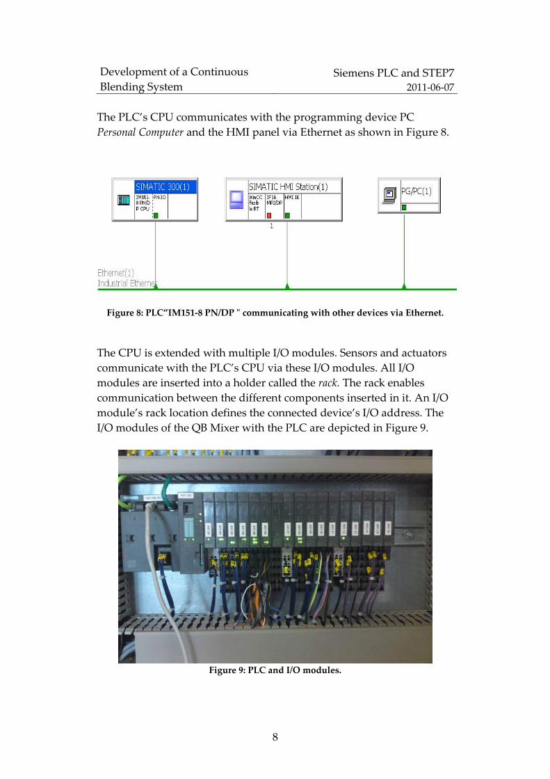
The PLC’s CPU communicates with the programming device PC

Personal Computer and the HMI panel via Ethernet as shown in Figure 8.

Figure 8: PLC”IM151‐8 PN/DP ʺ communicating with other devices via Ethernet.

The CPU is extended with multiple I/O modules. Sensors and actuators

communicate with the PLC’s CPU via these I/O modules. All I/O

modules are inserted into a holder called the rack. The rack enables

communication between the different components inserted in it. An I/O

module’s rack location defines the connected device’s I/O address. The

I/O modules of the QB Mixer with the PLC are depicted in Figure 9.

Figure 9: PLC and I/O modules.



2011‐06‐07

9

2.2 Analog Signals Signals that are continuous have an infinite number of states. These

variable signals need to be converted to digital signals by an A/D analog‐

to‐digital converter before CPU processing. This digitization is performed

inside an analog input interface within the I/O module. The analog

device’s current output is often transformed to a voltage by a built‐in

resistor. A common standard used in representing analog signals is

letting 4mA corresponds to the minimum signal level (1V) and 20mA

the maximum (5V). Digitized values corresponding to the continuous

values between 1‐5V are rated by the PLC’s CPU, values ranging above

or below are discarded by the CPU. A value < 0,296V is used for

detecting cable failure. Table 1 shows Siemens STEP7 format.

Measuring range 1 ‐ 5 V Decimal (value seen from

the CPU point of view)

Range

> 5,704 32767 Overflow

5,704

:

5,00014

32511

:

27649

Overrange

5,000

4,000

:

1,000

27648

20736

:

0

Rated range (normal

operation range)

0,99986

:

0,296

‐1

:

‐4864

Undershoot range

< 0,296 ‐32768 Underflow

Table 1: SIMATIC STEP7 format, measuring range 1‐5V.

Table 2 lists some devices that can be interfaced with analog input

modules.



2011‐06‐07

10

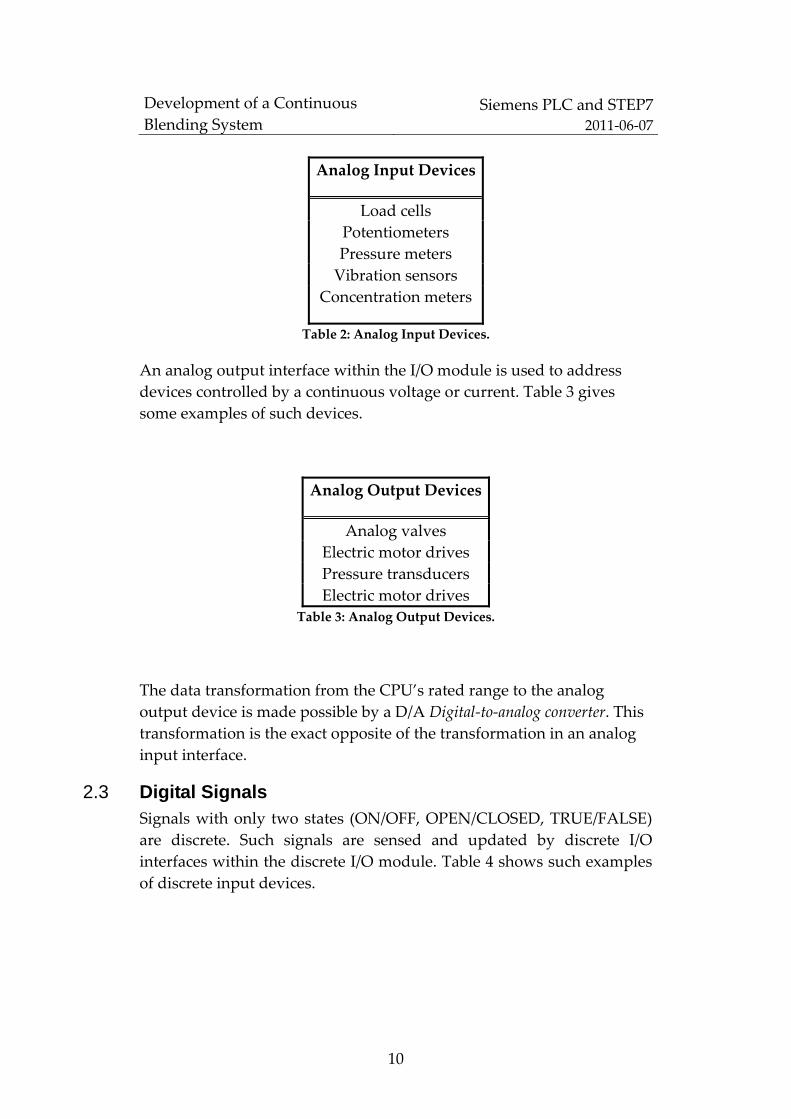
Analog Input Devices

Load cells

Potentiometers

Pressure meters

Vibration sensors

Concentration meters

Table 2: Analog Input Devices.

An analog output interface within the I/O module is used to address

devices controlled by a continuous voltage or current. Table 3 gives

some examples of such devices.

Analog Output Devices

Analog valves

Electric motor drives

Pressure transducers

Electric motor drives

Table 3: Analog Output Devices.

The data transformation from the CPU’s rated range to the analog

output device is made possible by a D/A Digital‐to‐analog converter. This

transformation is the exact opposite of the transformation in an analog

input interface.

2.3 Digital Signals Signals with only two states (ON/OFF, OPEN/CLOSED, TRUE/FALSE)

are discrete. Such signals are sensed and updated by discrete I/O

interfaces within the discrete I/O module. Table 4 shows such examples

of discrete input devices.



2011‐06‐07

11

Digital Input Devices

Level sensors

Motor contacts

Push buttons

Relay contacts

Circuit breakers

Table 4: Digital Input Devices.

Table 5 shows examples of discrete output devices

Digital Output Devices

Alarms

Motor startars

Lights

Fans

Control relays

Table 5: Digital Output Devices.

2.4 STEP7 STEP7 is the basic software package used to configure and program

SIMATIC PLCs. It consists of different applications, each performing a

specific task within the automated task, such as:

Configuring the hardware (PLC, I/O modules…etc).

Creating user programs and debugging

Networks configuration

The STEP7 Standard package applications (tools) are shown in Figure

10.



2011‐06‐07

12

Figure 10: STEP7 standard package [2].

2.4.1 SIMATIC Manager

The SIMATIC Manager is a GUI Graphical user interfaces provided to the

engineer to handle the applications (tools) of the STEP7 Standard

packages. It manages the editors of the programming languages,

integrate additional software package, operates and monitor HMI

systems, such as WinCC Windows Control Center and runtime software,

such as PID Control.

Figure 10: Some applications accessed by the SIMATIC Manager [2].



2011‐06‐07

13

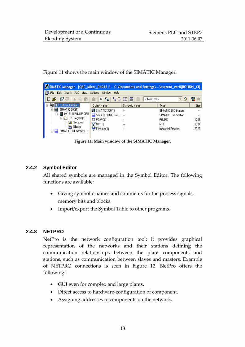
Figure 11 shows the main window of the SIMATIC Manager.

Figure 11: Main window of the SIMATIC Manager.

2.4.2 Symbol Editor

All shared symbols are managed in the Symbol Editor. The following

functions are available:

Giving symbolic names and comments for the process signals,

memory bits and blocks.

Import/export the Symbol Table to other programs.

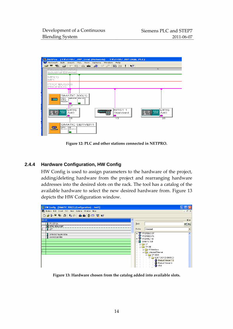
2.4.3 NETPRO

NetPro is the network configuration tool; it provides graphical

representation of the networks and their stations defining the

communication relationships between the plant components and

stations, such as communication between slaves and masters. Example

of NETPRO connections is seen in Figure 12. NetPro offers the

following:

GUI even for complex and large plants.

Direct access to hardware‐configuration of component.

Assigning addresses to components on the network.



2011‐06‐07

14

Figure 12: PLC and other stations connected in NETPRO.

2.4.4 Hardware Configuration, HW Config

HW Config is used to assign parameters to the hardware of the project,

adding/deleting hardware from the project and rearranging hardware

addresses into the desired slots on the rack. The tool has a catalog of the

available hardware to select the new desired hardware from. Figure 13

depicts the HW Cofiguration window.

Figure 13: Hardware chosen from the catalog added into available slots.



2011‐06‐07

15

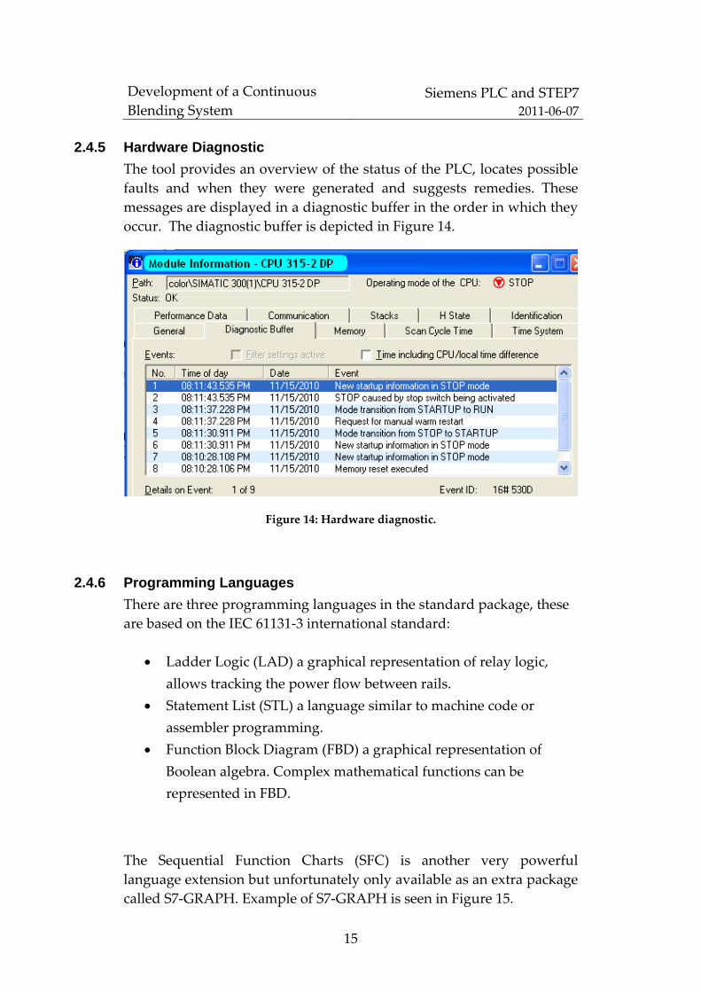
2.4.5 Hardware Diagnostic

The tool provides an overview of the status of the PLC, locates possible

faults and when they were generated and suggests remedies. These

messages are displayed in a diagnostic buffer in the order in which they

occur. The diagnostic buffer is depicted in Figure 14.

Figure 14: Hardware diagnostic.

2.4.6 Programming Languages

There are three programming languages in the standard package, these

are based on the IEC 61131‐3 international standard:

Ladder Logic (LAD) a graphical representation of relay logic,

allows tracking the power flow between rails.

Statement List (STL) a language similar to machine code or

assembler programming.

Function Block Diagram (FBD) a graphical representation of

Boolean algebra. Complex mathematical functions can be

represented in FBD.

The Sequential Function Charts (SFC) is another very powerful

language extension but unfortunately only available as an extra package

called S7‐GRAPH. Example of S7‐GRAPH is seen in Figure 15.



2011‐06‐07

16

Figure 15: sequential programming with S7‐GRAPH.

There is also a text based language, Structured Control Language S7‐

SCL that provides high‐level programming elements such as loops and

alternative branching. S7‐SCL is therefore suitable for programming

complex algorithms. S7‐SCL is available as an extra package to the

STEP7 Basic Package.

2.5 Human-Machine Interface, HMI PCs with better graphics than PLCs are increasingly being used as an

interface between operators and PLCs. A SCADA Supervisory Control

and Data Acquisition as the name implies is a higher level of supervised

control. An HMI system includes such an interface between the

operator and the machine/plant. Some basic tasks performed by the

HIM software are:

Process visualization

The plant is visualized on the HMI‐panel. The screen of the HMI

is updated dynamically.

Operator control of the plant

GUIs enable the operator to control different actuators and

devices.



2011‐06‐07

17

Displaying alarms

Critical states trigger alarms.

Archiving process values and alarms

HMI systems can log alarms and monitored process values.

Plant and machine parameter management

Plant and machines parameters can be stored in recipes.

Siemens offers a range of HMI and SCADA products. WinCC flexible

Advanced is used to configure the HMI panel of the QB Mixer. WinCC

flexible Advanced is integrated in the SIMATIC Manager; this enables

direct access to the STEP7 symbols and data blocks defined in the user

program. The basic package contains communication channels to

exchange data with the AS Automation System e.g. MPI, PROFIBUS‐DB

and TCP/IP (Ethernet). WinCC flexible Advanced has a powerful

simulator to simulate projects containing internal tags and process

values. The simulator enables debugging and testing without any

connected PLC and it also enables implementation of a project for demo

purposes. The main HMI‐panel window is depicted in Figure 16.

Figure 16: Starting window of the QB Mixerʹs HMI.



2011‐06‐07

18

2.6 The User Program The user program defines all the instructions and declarations needed to

control the automated task. User programs are interfaced with the

CPU’s OS via Organization Blocks. OBs are part of the user program and

are processed by the OS when specific events occur. Embedded in the

CPU’s OS are System Functions (SFCs) and System Function Blocks

(SFBs). Both types of blocks can be called by a user program to perform

certain tasks. User defined code (including calls to SFCs and SFBs) is

written in one of three block types Functions (FC), Function Blocks (FBs)

and OBs. SFBs and FBs require that data must be available from one call

to the next‐call, this implies the need for memory. Memory

requirements are handled by System Data Blocks (SDBs) or Data Blocks

(DBs). A DB in STEP7 is a container for storing shared data, variables

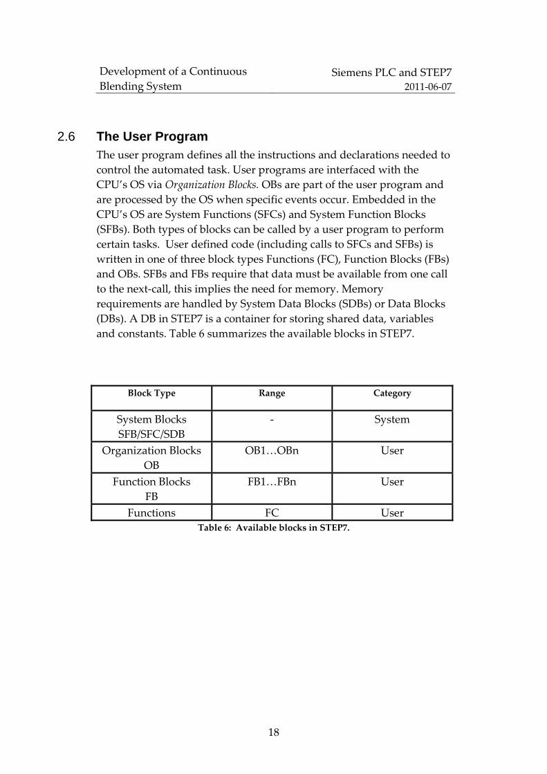
and constants. Table 6 summarizes the available blocks in STEP7.

Block Type Range Category

System Blocks

SFB/SFC/SDB

‐ System

Organization Blocks

OB

OB1…OBn User

Function Blocks

FB

FB1…FBn User

Functions FC User

Table 6: Available blocks in STEP7.



2011‐06‐07

19

After power up, the CPU initiate the startup program by reading the

instructions programmed in specific OBs (e.g. OB100). When the

execution of the startup OBs is finished the CPU begins processing the

main program (located in OB1). OB1 has the lowest processing priority.

This allows it to be interrupted by other events or OBs (e.g. error

events). The CPU processes OB1 cyclically, which is the “normal” type

of processing in PLCs based CPUs. A user program can therefore

entirely be programmed inside OB1 (not good practice). The

programmer usually defines subtasks using modular blocks of code,

such as FCs or FBs. All these “structures “can be called from OB1 and in

turn call other “structures” as depicted in Figure 17.

Figure 17: OS calling different OBs. They in turn call other user/system blocks.



2011‐06‐07

20

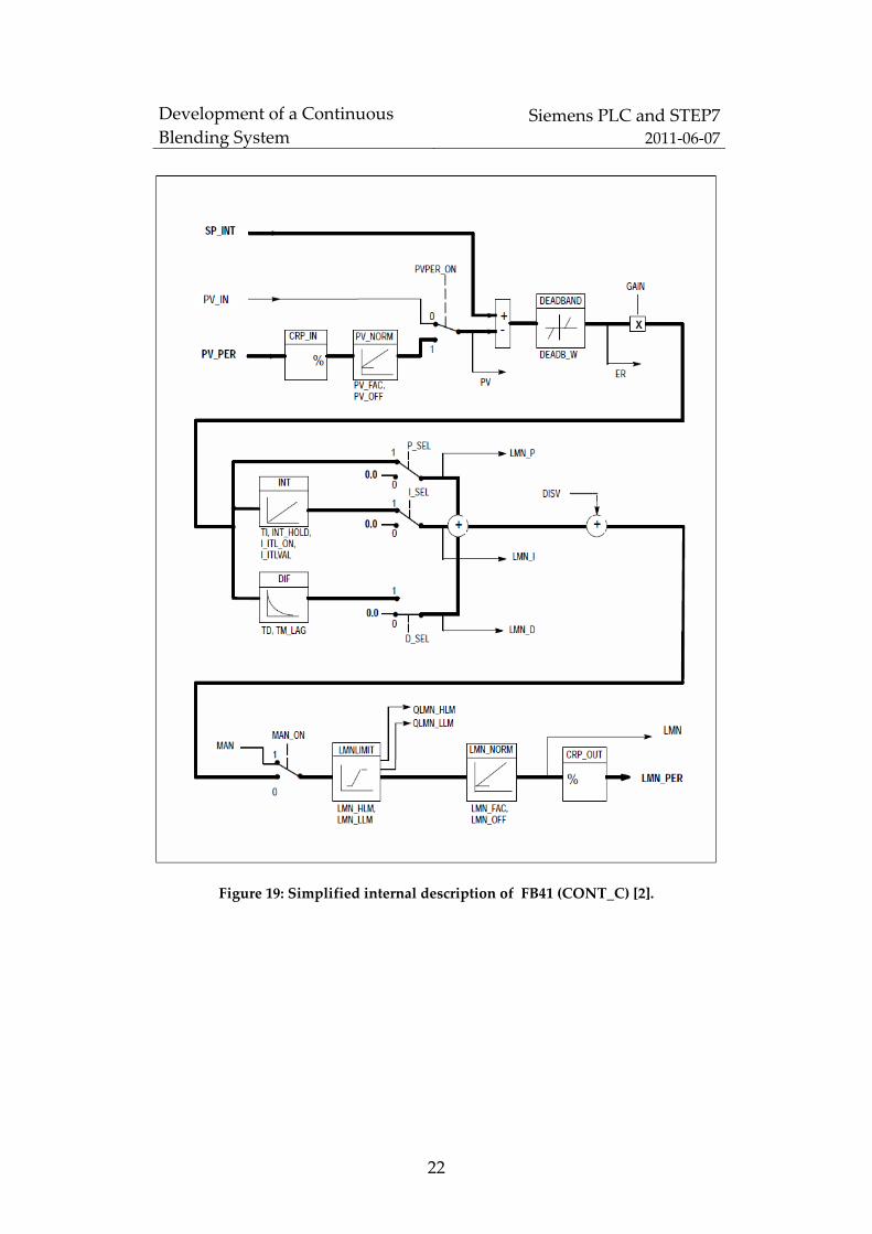
2.7 PID Control Controlling a plant variable (for example keeping a fixed pressure,

concentration or level) usually is done using a feedback strategy where

the actual value is fed back from the plant and compared to the

desired value upon which a controller output u is calculated. A

typical feedback block diagram is depicted in Figure 18.

Figure 18: Feedback loop.

The controller is said to be a PID controller if the control signal

consists of the sum of three terms: the P‐term (provides immediate

response to the control error), the I‐term (reacts to the accumulation of

errors), and the D‐term (responds to the rate at which the error is

changing). The “textbook” variant of the algorithm can be described as:

Where is the control signal and is the controller error

( ). The PID controller parameters are proportional



2011‐06‐07

21

gain , integral time and derivative time . The actual version of

the algorithm used in PLCs to achieve PID control is sampled with

intervals and can be expressed as:

Here is the control variable ( in the continuous version), is

the setpoint and is the process value.

The standard STEP7 package provides two software controllers

implemented as function Blocks (FBs), one for continuous‐control FB41

(CONT_C) and one for step‐control FB42 (CONT_S). These controllers

must be called at exactly equal intervals. A cyclic interrupt OB, e.g.

OB35, can be used as a “container” of the PID blocks. This avoids errors

and gives high accuracy in the internal calculations of the PID dynamics

(Integral/Derivative calculations). The PLC programmer can choose the

PID parameters needed for a certain plant control by activating or

deactivating the relevant PID parameters (for example PI‐control only).

One can even connect a plant disturbance variable (if it can be

measured) to the PID‐block to counteract noise. There is the option of

determining a dead band (implemented to suppress small error signals)

to avoid output oscillation and in turn actuator wear and tear. An

overview of the block diagram of a continuous PID is depicted in Figure

19.



2011‐06‐07

22

Figure 19: Simplified internal description of FB41 (CONT_C) [2].



2011‐06‐07

23

A description of the main parameters is given in Table 7.

Parameter Range of

Values Description

SP_INT ‐100.0...100. INTERNAL SETPOINT

The “internal setpoint” input is used to specify a setpoint

PV_IN ‐100.0...100.

PROCESS VARIABLE IN

An initialization value can be set at the “process variable

in” input or an external process variable in floating point

format can be connected.

CYCLE >=1ms

SAMPLING TIME

The time between the block calls must be constant. The

“sampling time “ input specifies the time between block

calls.

GAIN

PROPORTIONAL GAIN

The “proportional value” input specifies the controller

gain.

TI >= CYCLE

RESET TIME

The “reset time” input determines the time response of

the integrator.

TD >= CYCLE

DERIVATIVE TIME

The “derivative time” input determines the time response

of the derivative unit.

TM_LAG >= CYCLE/2

TIME LAG OF THE DERIVATIVE ACTION

The algorithm of the D action includes a time lag that can

be assigned at the “time lag of the derivative action”

input.

DEADB_W >= 0.0

DEAD BAND WIDTH

A dead band is applied to the error. The “dead band

width” input determines the size of the dead band.

DISV ‐100.0...100

DISTURBANCE VARIABLE

For feedforward control, the disturbance variable is

connected to input “disturbance variable”.

LMN OUTPUT VARIABLE MANIPULATED VALUE The effective manipulated value is output in floating point format at the “manipulated value” output.

Table 7: Main parameters of FB41 (CONT_C).


Blending System Method and Implementation

2011‐06‐07

24

3 Method and Implementation This chapter describes how the problem of developing the new mixer

was tackled, the possible approaches and their relationship to control

theory.

3.1 Possible solutions Analysis of the QB Mixer explained in chapter 1 reduced the problem to

“controlling the output’s concentration” with the minimum possible

change to the QB Mixer structure. Expanding the QB Mixer with extra

pipe‐work and valves enabling it to handle multiple input streams, one

for the solvent and one a feedback controlled input (output fed back

again if the desired concentration value was not met) was discarded.

Therefore only single‐input and single‐output (SISO) based solutions

were investigated. It was early decided that a concentration meter was

needed. Two approaches were presented to the company QB Food Tech

of which one was chosen.

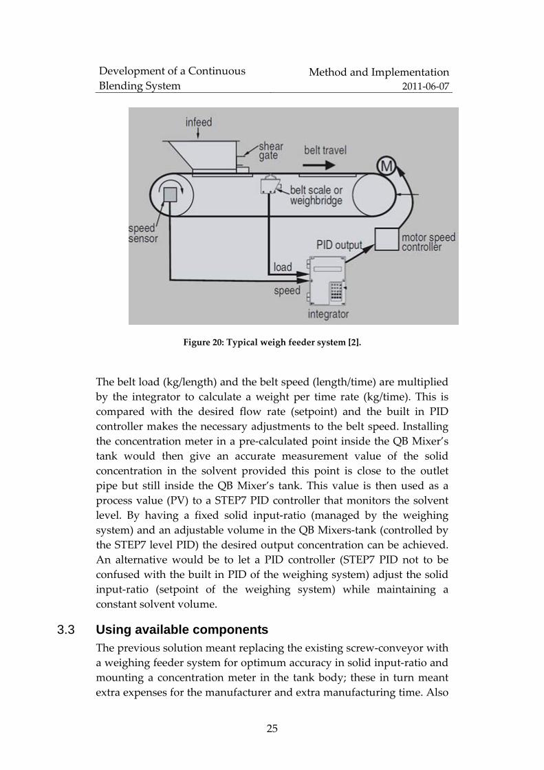
3.2 Weighing system with concentration meter In order to achieve exact accuracy in dosing a weighing feeder system

was suggested to replace the screw‐conveyor for delivering the solid

mass. A typical weigh feeder depicted in Figure 20, consists of three

parts:

Weight and speed sensing mechanisms.

Electronics for control such as built in PID.

Mechanical conveyor system.



2011‐06‐07

25

Figure 20: Typical weigh feeder system [2].

The belt load (kg/length) and the belt speed (length/time) are multiplied

by the integrator to calculate a weight per time rate (kg/time). This is

compared with the desired flow rate (setpoint) and the built in PID

controller makes the necessary adjustments to the belt speed. Installing

the concentration meter in a pre‐calculated point inside the QB Mixer’s

tank would then give an accurate measurement value of the solid

concentration in the solvent provided this point is close to the outlet

pipe but still inside the QB Mixer’s tank. This value is then used as a

process value (PV) to a STEP7 PID controller that monitors the solvent

level. By having a fixed solid input‐ratio (managed by the weighing

system) and an adjustable volume in the QB Mixers‐tank (controlled by

the STEP7 level PID) the desired output concentration can be achieved.

An alternative would be to let a PID controller (STEP7 PID not to be

confused with the built in PID of the weighing system) adjust the solid

input‐ratio (setpoint of the weighing system) while maintaining a

constant solvent volume.

3.3 Using available components The previous solution meant replacing the existing screw‐conveyor with

a weighing feeder system for optimum accuracy in solid input‐ratio and

mounting a concentration meter in the tank body; these in turn meant

extra expenses for the manufacturer and extra manufacturing time. Also



2011‐06‐07

26

a concern about the structural integrity of the QB Mixer existed because

of the drilling needed to mount the concentration meter. Therefore a

solution involving only the existing components and at the same time

showing a working principle of the new QB Mixer was developed. The

manufacturer then has the flexibility to decide on future upgrades based

on the correct verified functionality.

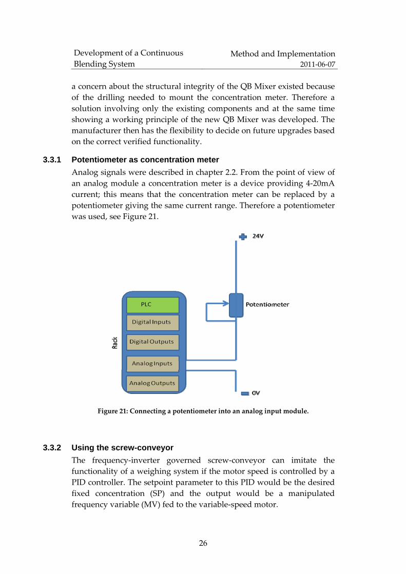
3.3.1 Potentiometer as concentration meter

Analog signals were described in chapter 2.2. From the point of view of

an analog module a concentration meter is a device providing 4‐20mA

current; this means that the concentration meter can be replaced by a

potentiometer giving the same current range. Therefore a potentiometer

was used, see Figure 21.

Figure 21: Connecting a potentiometer into an analog input module.

3.3.2 Using the screw-conveyor

The frequency‐inverter governed screw‐conveyor can imitate the

functionality of a weighing system if the motor speed is controlled by a

PID controller. The setpoint parameter to this PID would be the desired

fixed concentration (SP) and the output would be a manipulated

frequency variable (MV) fed to the variable‐speed motor.



2011‐06‐07

27

The new system (consisting of a potentiometer and the screw‐motor)

was implemented with the process output variable (OUTV) simulated

by a potentiometer. The new solution was tested to verify its

functionality. It consists of three basic modes Pre PID, PID and

Termination, see Figure 21.

Figure 22: Three basic modes.

Pre PID mode calculates a concentration by letting the

screw conveyor run a certain time and filling the tank with

a fixed volume of the solvent.

In PID mode the programmed PID takes over when the

QB Mixer’s outlet is enabled and compares the setpoint

with the process value (the output of a potentiometer). The

PID keeps adjusting the manipulated variable (speed of

the screw conveyor) based on the read output. This mode

will keep running until terminated.



2011‐06‐07

28

Termination mode ends PID control.

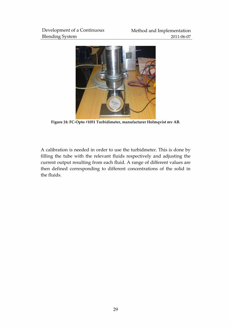
3.4 Turbidimeter The discussion through chapters 3.1, 3.2 and 3.3 showed a working

solution. The next step was to replace the potentiometer with a

concentration meter of choice to be mounted on an outlet pipe. A meter

measuring turbidity was chosen. A basic turbidimeter consists of a light

source for illuminating the measured sample (fluid) and photoelectric

sensors with current/voltage output to indicate light intensity. A

turbidimeter works by measuring the intensity of the scattered light

and/or transmitted light. Light scatters differently depending on the

particles’ sizes relative to the wavelength of the lightsource, see Figure

23.

Figure 23: Working principle of a turbidimeter.

The actual turbidimeter used utilizes only one scattered light detector

with an output range of 4‐20mA. In a dairy product let say milk, higher

fat content will reflect more light back to the detector and indicate a

higher output signal level than lower fat content. Figure 24 shows the

used Turbidimeter .



2011‐06‐07

29

Figure 24: FC‐Opto #1051 Turbidimeter, manufacturer Holmqvist mv AB.

A calibration is needed in order to use the turbidmeter. This is done by

filling the tube with the relevant fluids respectively and adjusting the

current output resulting from each fluid. A range of different values are

then defined corresponding to different concentrations of the solid in

the fluids.


Blending System Modeling the Mixer

2011‐06‐07

30

4 Modeling the Mixer This chapter presents a brief introduction to the modeling procedure

used, followed by a simplified yet accurate mathematical model of the

concentration change in the mixer based on data obtained from

experiments. The model is then used to obtain the necessary PID

parameters based on the Cohen‐Coon method described in many

textbooks [9, 10].

4.1 Mathematical modeling Finding a mathematical model describing a certain plant is a good

starting point in achieving the control task. In general there are three

main steps in developing such models for physical systems:

1. Defining system boundaries. Physical systems interact

with other systems. Therefore it is necessary to recognize

relevant boundaries of the system being modeled.

2. Making assumptions. For the sake of simplification

assumptions are made. One example is assuming the same

concentration throughout a volume in a mixing tank

(homogenous conditions in the tank).

3. Using the conservation of mass and energy law. The

balance law states: the rate of change of inventory in the

system = (rate of inflows) – (rate of outflows) + (rate of generated

inventory) – (rate of consumed inventory). Inventory is a

general term. It can refer to mass, momentum or electrical

charge. Using the law results in a set of ordinary

differential equations.

Keeping these steps in mind one starts developing a model for the

concentration change inside the QB Mixer by assuming that the

blending in the mixer’s tank has a constant volume (achieved by

level control), the solvent does not contain component A and the

homogenous condition is satisfied (perfect stirring assumption ).

Symbols are shown in Figure 25.



2011‐06‐07

31

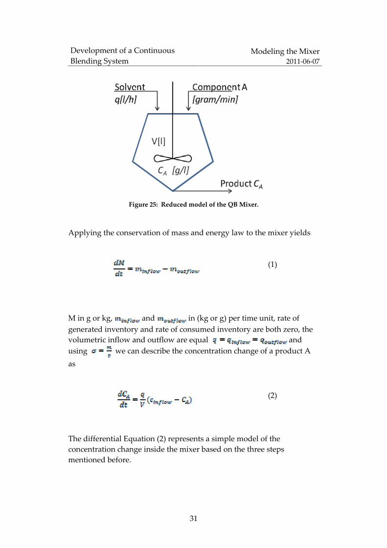
Figure 25: Reduced model of the QB Mixer.

Applying the conservation of mass and energy law to the mixer yields

(1)

M in g or kg, and in (kg or g) per time unit, rate of

generated inventory and rate of consumed inventory are both zero, the

volumetric inflow and outflow are equal and

using we can describe the concentration change of a product A

as

The differential Equation (2) represents a simple model of the

concentration change inside the mixer based on the three steps

mentioned before.

(2)



2011‐06‐07

32

4.2 First-order system plus dead time The input/output relationship of the system can be expressed by a

transfer function G(s) defined in the Laplace domain. With as U

the Laplace transform of (2) is written as:

(3)

The ratio is called the time constant and is used to describe how

fast the process variable changes in response to a change in controller

output “time from first measured change in process output to 63% of

final change in value”. A large time constant translates into a slow PV

response. Equation (3) reveals that the Mixer is a first‐order system, but

in reality such systems always has time delays and process gain. A more

accurate modelling would be the first order system plus dead time

FOPDT expressed as:

(4)



2011‐06‐07

33

where K is a scaling factor “change in process output divided by change

in process input”, is the time constant and is the time delay, defined

as the time from the introduction of a change in an input until the

measured output first begins to respond ”also called the deadtime” .

These three parameters fully capture the dynamics of the process. The

process reaction curve for an FOPDT system can be experimentally

obtained. An example of such a curve is depicted in Figure 26.

Figure 26: FOPDT curve.

In order to find the parameters an open loop experiment recording the

Mixer’s transfer function was conducted. The Mixer’s concentration

output was kept constant by letting the level controller PID maintain a

certain level “volume” of the solvent inside the mixer, and letting the



2011‐06‐07

34

screw‐conveyor run with a constant frequency. This corresponds to

finding , and . A step change in the screw‐conveyor’s frequency

was introduced “ ” at time to start the remaining parameter

reorganization procedure. , and could now be determined.

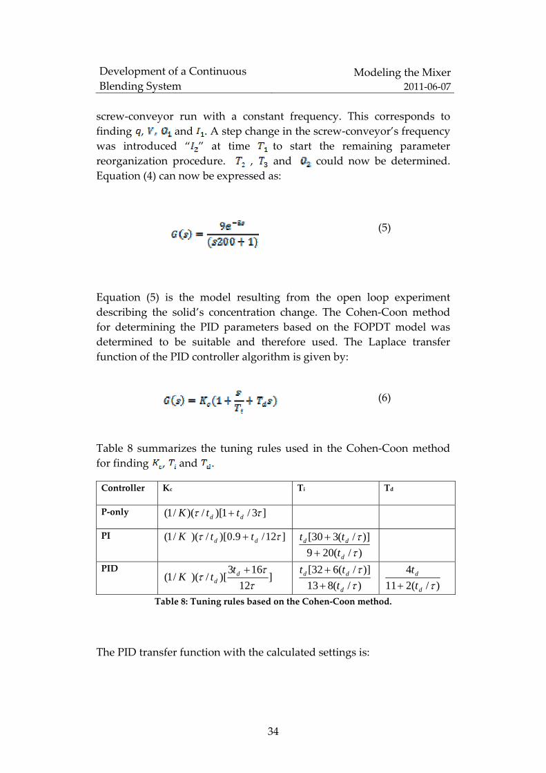
Equation (4) can now be expressed as:

(5)

Equation (5) is the model resulting from the open loop experiment

describing the solid’s concentration change. The Cohen‐Coon method

for determining the PID parameters based on the FOPDT model was

determined to be suitable and therefore used. The Laplace transfer

function of the PID controller algorithm is given by:

(6)

Table 8 summarizes the tuning rules used in the Cohen‐Coon method

for finding , and .

Controller Kc Ti Td

P‐only ]3/1)[/)(/1( dd ttK

PI ]12/9.0)[/)(/1( dd ttK

)/(209

)]/(330[

d

dd

t

tt

PID ]

12

163)[/)(/1(

d

d

ttK

)/(813

)]/(632[

d

dd

t

tt

)/(211

4

d

d

t

t

Table 8: Tuning rules based on the Cohen‐Coon method.

The PID transfer function with the calculated settings is:



2011‐06‐07

35

(7)

Equation (5) and (7) are simulated in a closed‐loop system in Simulink

as depicted in Figure 27.

Figure 27: Simulink model of the PID controller and the FOPDT system.

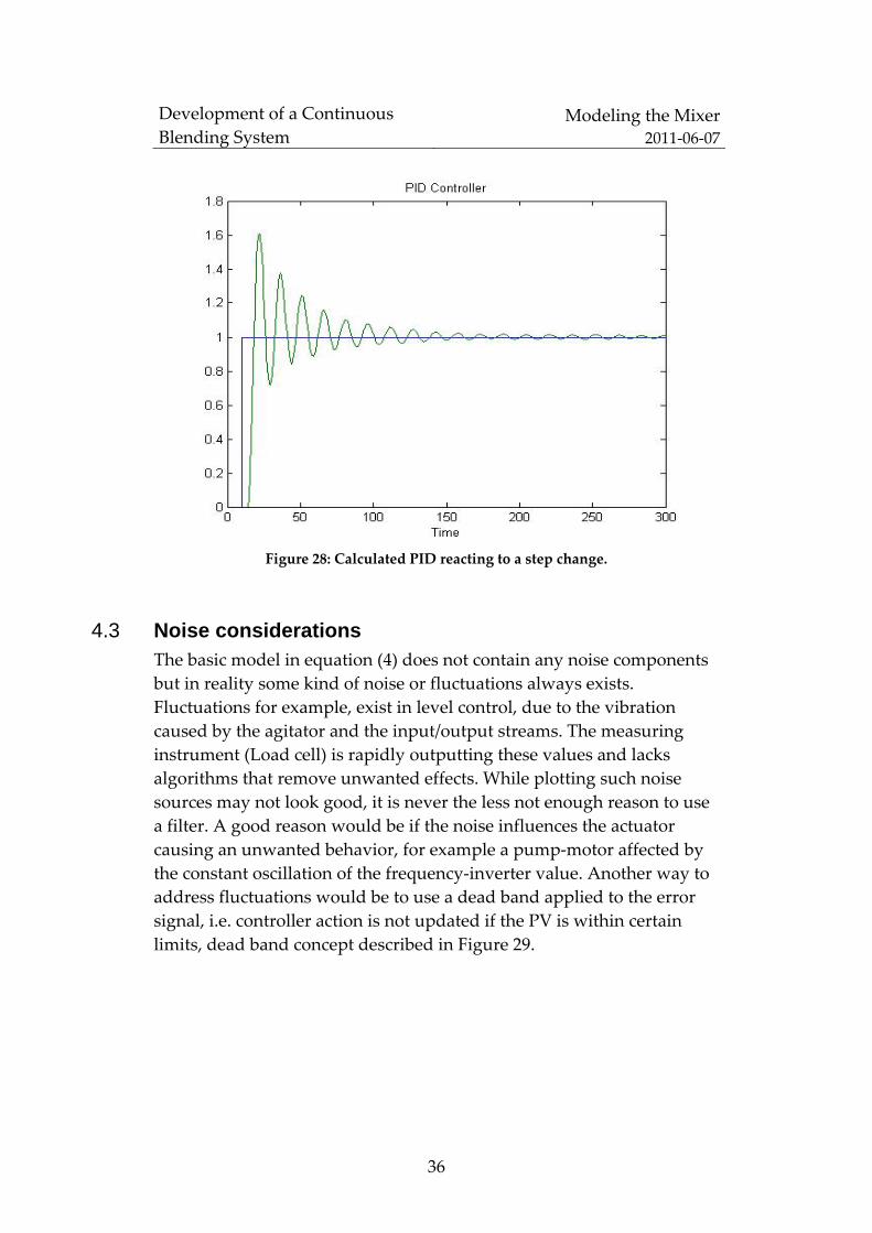
Figure 28 shows the Simulink PID with the calculated settings reacting

to a setpoint change in the solid’s concentration.



2011‐06‐07

36

Figure 28: Calculated PID reacting to a step change.

4.3 Noise considerations The basic model in equation (4) does not contain any noise components

but in reality some kind of noise or fluctuations always exists.

Fluctuations for example, exist in level control, due to the vibration

caused by the agitator and the input/output streams. The measuring

instrument (Load cell) is rapidly outputting these values and lacks

algorithms that remove unwanted effects. While plotting such noise

sources may not look good, it is never the less not enough reason to use

a filter. A good reason would be if the noise influences the actuator

causing an unwanted behavior, for example a pump‐motor affected by

the constant oscillation of the frequency‐inverter value. Another way to

address fluctuations would be to use a dead band applied to the error

signal, i.e. controller action is not updated if the PV is within certain

limits, dead band concept described in Figure 29.



2011‐06‐07

37

Figure 29: Dead band applied to the error signal ER.

Other causes of noise might be introduced mechanically (vibrations) or

electrically (environment). Noise coming from the measurement and

process can cause the controller to fluctuate as changes in the error

caused by the noise are amplified by the PID’s derivative term making

the entire control system sensitive to disturbances. Reduction of noise

might not be needed if the controller gain is small and the derivative

term can be omitted yielding a PI‐controller. If not, noise can be

minimized using a low‐pass filter to exclude high frequency

components or by an exponential filter to smooth the signal. The

standardized first‐order exponential smoothing filter is described as:



2011‐06‐07

38

(8)

where is the current filter output, is the previous output and

is the current input. The parameter is a tuning parameter chosen in the

range 0 to 1. In STEP7 signal processing is allowed on analog variables

by the built in lead‐lag compensator algorithm implemented as a

function block (FB80) that is available to the programmer in the

standard STEP7 library. The algorithm is implemented as:

(9)

where is the lag time, is the lead time and is the sampling

time. The exponential filter equation (8) can be derived from equation

(9) by setting the lead time to 0 and defining . The parameter

can then be set to ‐1 achieving (8). The noise suppressor/filter is now

expressed as

(10)

Equation (10) was implemented in STEP7 as an extra option in case the

dead band concept used to handle noise/ fluctuations would be

insufficient.


Blending System Program Design

2011‐06‐07

39

5 Program Design This chapter describes the main program structures used in this project

and shows some results and the real time working solution.

5.1 Time representation Time representation issues were addressed by using the built‐in clock

memory byte from the CPU, each bit in the byte is assigned a specific

frequency. Table 9 shows the assigned values for each bit in the byte.

Bit of the Clock Memory Byte

7 6 5 4 3 2 1 0

Period Duration (s)

2.0

1.6

1.0

0.8

0.5

0.4

0.2

0.1

Frequency (Hz)

0.5

0.625

1

1.25

2

2.5

5

10

Table 9: Bits values in the memory byte.

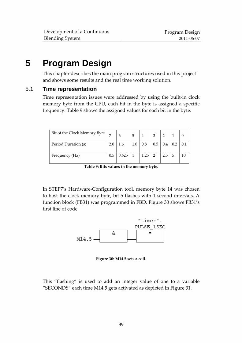
In STEP7’s Hardware‐Configuration tool, memory byte 14 was chosen

to host the clock memory byte, bit 5 flashes with 1 second intervals. A

function block (FB31) was programmed in FBD. Figure 30 shows FB31’s

first line of code.

Figure 30: M14.5 sets a coil.

This “flashing” is used to add an integer value of one to a variable

“SECONDS” each time M14.5 gets activated as depicted in Figure 31.



2011‐06‐07

40

Figure 31: A pulse is detected every time M14.5 is activated.

When “SECONDS” equals 60 then one minute has elapsed and

“SECONDS” should be reset to zero, as seen in Figure 32.

Figure 32: Moving a value of zero to ʺSECONDSʺ.

The same principle is used to address minutes and hours, each having

their respective variable “MINUTES” and “HOURS”. The total time

elapsed is converted to seconds via a Function (FC2) that is called from

inside FB31. Figure 33 shows FC2’s interface.



2011‐06‐07

41

Figure 33: FC2 outputs time in seconds.

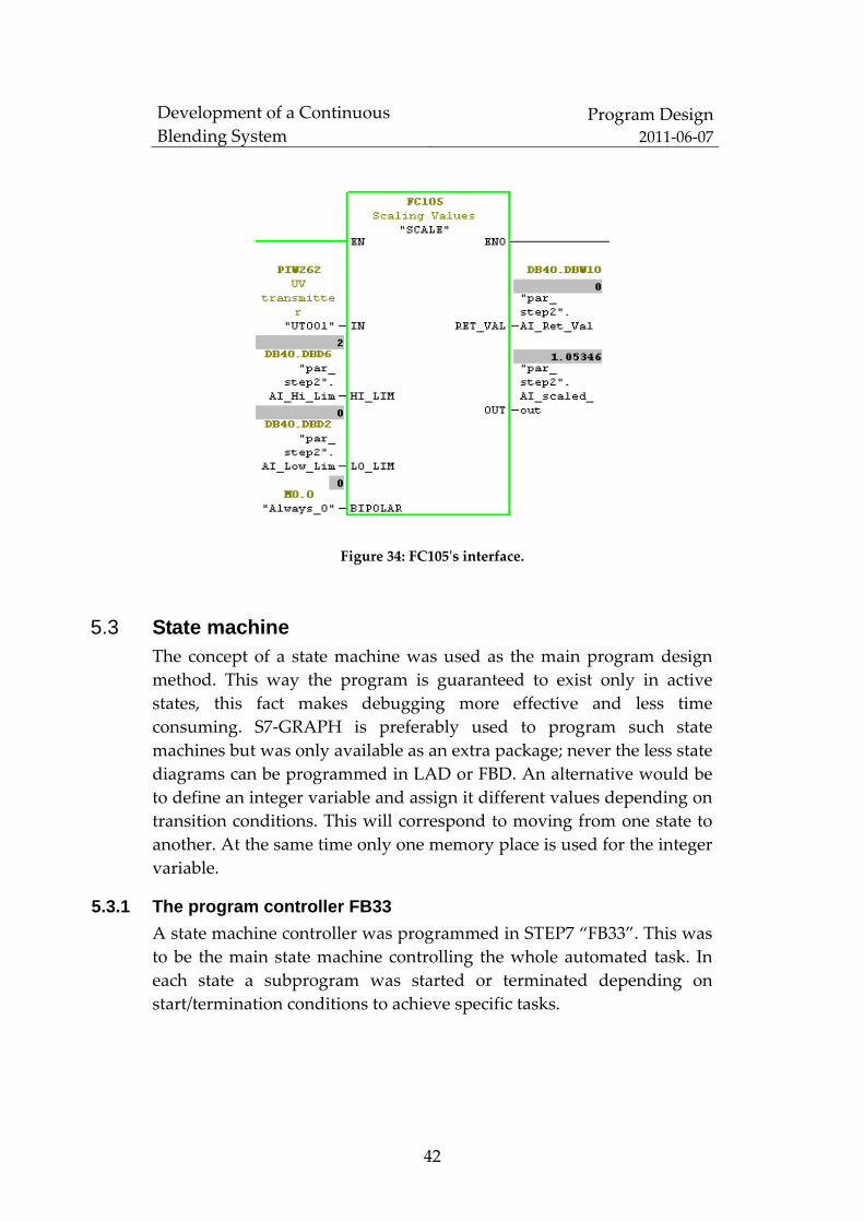
5.2 Scaling Analog signals are scaled using the “SCALE” function FC105. The

function takes an input IN as an integer and converts it to a real value

between two limits, a low and a high limit (LO_LIM and HI_LIM). The

equation used is:

The constants K1 and K2 are set based upon whether the input value is

bipolar or unipolar. If bipolar is chosen then the input integer value is

assumed to be between –27648 and 27648, therefore, K1 = –27648.0 and

K2 = +27648.0. If unipolar is chosen then the input integer value is

assumed to be between 0 and 27648, therefore, K1 = 0.0 and K2 =

+27648.0. Figure 34 shows the FC105’s interface.



2011‐06‐07

42

Figure 34: FC105ʹs interface.

5.3 State machine The concept of a state machine was used as the main program design

method. This way the program is guaranteed to exist only in active

states, this fact makes debugging more effective and less time

consuming. S7‐GRAPH is preferably used to program such state

machines but was only available as an extra package; never the less state

diagrams can be programmed in LAD or FBD. An alternative would be

to define an integer variable and assign it different values depending on

transition conditions. This will correspond to moving from one state to

another. At the same time only one memory place is used for the integer

variable.

5.3.1 The program controller FB33

A state machine controller was programmed in STEP7 “FB33”. This was

to be the main state machine controlling the whole automated task. In

each state a subprogram was started or terminated depending on

start/termination conditions to achieve specific tasks.



2011‐06‐07

43

To initialize the starting data and the first state a first scan signal was

used from the PLC’s CPU. State 1 is a waiting state. If a starting signal is

detected from the HMI “Global Start” State 2 is activated, state 2 is an

initial dosing state that activates the filling of the solvent and the screw‐

conveyer to achieve a first acceptable concentration of the solid in the

solvent before the concentration PID that is activated in State 3 takes

over. A representation of FB33 is shown in Figure 35.

Figure 35: FB33 called from OB1 (left) and its internal states (right).

Communication between FB33 and the two subroutines is depicted in

Figure 36.



2011‐06‐07

44

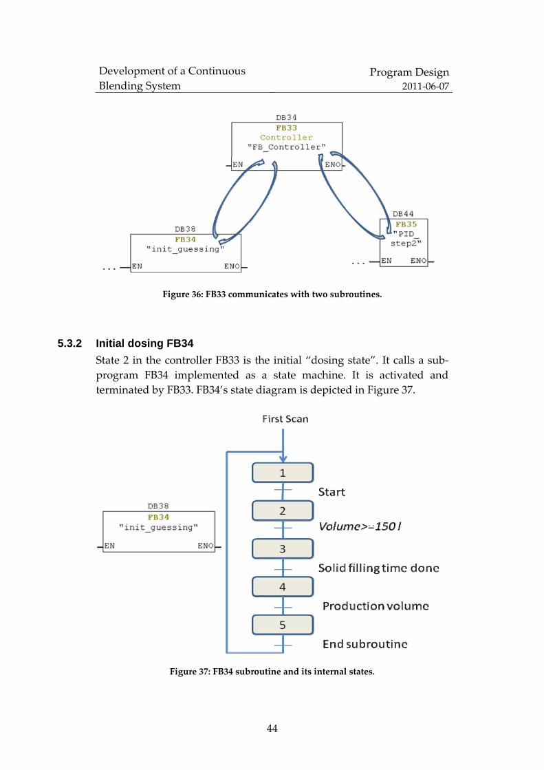
Figure 36: FB33 communicates with two subroutines.

5.3.2 Initial dosing FB34

State 2 in the controller FB33 is the initial “dosing state”. It calls a sub‐

program FB34 implemented as a state machine. It is activated and

terminated by FB33. FB34’s state diagram is depicted in Figure 37.

Figure 37: FB34 subroutine and its internal states.



2011‐06‐07

45

The main tasks of the FB34’s states are:

State 1 waits on the start signal from the main controller.

State 2 activates the solvent filling signal and monitors the

solvent level on receiving the “Start condition “. A fixed

volume level is the transition condition to the next state.

State 3 activates the timer –subroutine FB31, the dispersion

tool and the screw conveyor signal.

State 4 disables the screw‐conveyor signal and waits for

the filling volume to reach a predetermined production

volume.

State 5 signals to the main controller FB33 that the dosing

subroutine FB34 is done and waits for acknowledgment.

5.3.3 Concentration PID FB35

The concentration PID FB35 receives a “Start PID” signal from the main

controller FB33 when the initial dosing subroutine is terminated. FB35’s

state diagram is depicted in Figure 38.

Figure 38: FB35 subroutine and its internal states.



2011‐06‐07

46

The main tasks of the FB35’s states are:

State 1 is activated by the first scan signal. It waits for the

“Start PID “signal.

State 2 enables the concentration PID block in OB35.

State 3 ends the subroutine.

5.4 Interrupt routine OB35 As mentioned in chapter 2.7, PID blocks must be programmed in

interrupt routines. This is provided as cyclic interrupt OBs in STEP7. To

start an OB interrupt the interval must be specified as a whole multiple

of the basic clock rate of 1ms.

To avoid interrupt OBs being started at the same time point a phase

offset can be specified. This will delay the execution of a cyclic OB

interrupt by a specific time after the interrupt time (Interval) has expired.

Two PIDs were programmed in OB35: the PID controlling the output

pump‐motor (PM002) by controlling its frequency inverter (SC002) and

the PID controlling the Screw conveyer motor (PM004) by adjusting its

frequency inverter SC004. OB35’s interval was 100ms. This corresponds

to the parameter CYCLE, the sampling time in a continuous PID block

“FB41”. The Phase offset option was not adjustable in the PLC’s CPU.

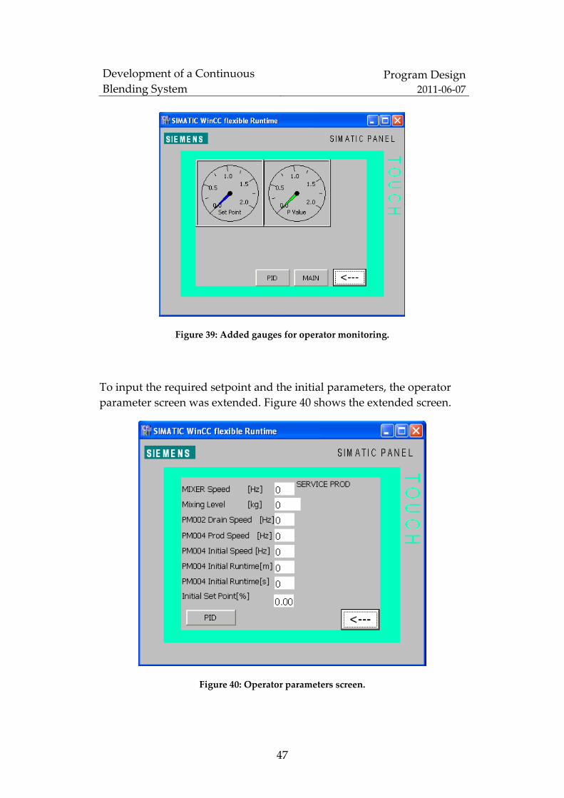
5.5 HMI The concentration of the solid in the solvent needs to be monitored by

the operator. Two gauges, one for the setpoint and one for process

value, were added in a new “screen“ in WinCC flexible Advanced to

achieve this, as shown in Figure 39.



2011‐06‐07

47

Figure 39: Added gauges for operator monitoring.

To input the required setpoint and the initial parameters, the operator

parameter screen was extended. Figure 40 shows the extended screen.

Figure 40: Operator parameters screen.



2011‐06‐07

48

5.6 Running the program The PID Control Parameter Assignments user interface is part of STEP7.

It has a limited plotting functionality to view PID parameters in real‐

time. This was used to check for noise and decide if further adjustments

were needed.

Figure 41 shows how the level PID output “manipulated value”

stabilizes after applying the dead band. The output pump‐motor

(PM002) is running steady and with minimum risk of wear and tear.

Figure 41: Dead band applied at 15:23:45 stabilizes PM002 (purple), process value

(green) and setpoint (pink).

Figure 42 shows how a solids concentration of 1% is maintained by the

concentration PID. The concentration PID output “manipulated value”

is kept steady by the applied dead band. The screw‐conveyor is running

on a very low frequency, less than 3% of its 50 Hz.



2011‐06‐07

49

Figure 42: Concentration PID maintaining 1% as required.


Blending System Conclusions

2011‐06‐07

50

6 Conclusions The solution provided for the company QB Food Tech fulfils the

required specifications; by feeding back the measured signal from the

Turbidimeter to a PID controller the desired solids concentration can be

maintained. A continuous blending system was developed starting from

a batch process without adding extra expenses for the company. Other

possible solutions were suggested too and briefly discussed.


Blending System Conclusions

2011‐06‐07

51

7 Further Development Although the solution implemented fulfils the requirements, there are

some areas that need to be investigated in future work, i.e. the effect of

the agitator speed on the dissolution of the solid substances in the

solvent. Implementing the vacuum function in a continuous blending

system is another area that needs to be balanced with the overall

solution. Finally a mathematical model of the flow fields inside the QB

Mixer’s is needed to investigate their influence on how well the

dissolution of the dissolution of the solid substances.


Blending System References 2011‐06‐07

52

References

[1] QB Food Tech,”QB MIXER”, http://www. qbfoodtech.se

[2] SIEMENS, “Automation Technology”, www.siemens.com

[3] Hans Berger, Automating with Simatics. Third edition. Germany:

Publicis Corporate Publishing, 2006.

[4] Siemens, 2006: Simatic Working with STEP7 Getting Started module.

(6ES7810‐4CA08‐8BW0).

[5] Siemens, 2008: ET 200S distributed I/O 2AI U HS analog electronic

module. (6ES7134‐4FB52‐0AB0).

[6] J. Müller, Controlling with Simatic. Germany: Publicis Corporate

Publishing, 2006.

[7] Siemens: Simatic Standard Software for S7‐300 and S7‐400 PID

Control module. (C79000‐G7076‐C516‐01).

[8] Terrence Blevins and Mark Nixon, Control Loop Foundation‐Batch

and Continuous Processes. USA: ISA.

[9] K.J. Åström and T. Högglund, Automatic Tuning of PID

Controllers, second edition. Research Triangle Park, NC: ISA

Press, 1995.

[10] Michael King, Process Control: A practical Approach. United

Kingdom: John Wiley & Sons Inc.

[11] Cecil L. Smith, Practical Process Control: Tuning and

Troubleshooting. USA: John Wiley & Sons Inc.

[12] EA. Parr, Programmable Controllers An engineer’s guide. Third

edition. Great Britain: Newnes publications, 2003.

[13] LA. Bryan, Programmable Controllers Theory and Implementation.

Second edition. USA: Industrial Text, 1997.

Development of a Continuous Blending System1 - … document/5282_full...Development of a Continuous...

Documents

Transcript of Development of a Continuous Blending System1 - … document/5282_full...Development of a Continuous...