Development of a 3D fractal cirrus model and its use in ... · Development of a 3D fractal cirrus...
92
Development of a 3D fractal cirrus model and its use in investigating the impact of cirrus inhomogeneity on radiation Sarah Kew August 2003 Submitted to the Department of Mathematics University of Reading in partial fulfil- ments of the requirements for the degree of Master of Science. I confirm that this is my own work and the use of all material from other sources has been properly and fully acknowledged. i
Transcript of Development of a 3D fractal cirrus model and its use in ... · Development of a 3D fractal cirrus...
Development of a 3D fractal cirrus model and its
use in investigating the impact of cirrus
inhomogeneity on radiation
Sarah Kew
August 2003
Submitted to the Department of Mathematics University of Reading in partial fulfil-
ments of the requirements for the degree of Master of Science.
I confirm that this is my own work and the use of all material from other sources has
been properly and fully acknowledged.
i
ii
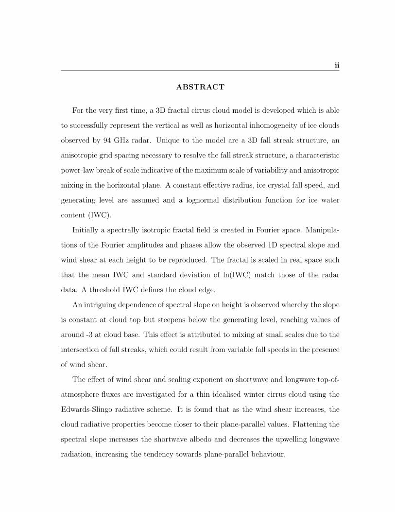
ABSTRACT
For the very first time, a 3D fractal cirrus cloud model is developed which is able
to successfully represent the vertical as well as horizontal inhomogeneity of ice clouds
observed by 94 GHz radar. Unique to the model are a 3D fall streak structure, an
anisotropic grid spacing necessary to resolve the fall streak structure, a characteristic
power-law break of scale indicative of the maximum scale of variability and anisotropic
mixing in the horizontal plane. A constant effective radius, ice crystal fall speed, and
generating level are assumed and a lognormal distribution function for ice water
content (IWC).
Initially a spectrally isotropic fractal field is created in Fourier space. Manipula-
tions of the Fourier amplitudes and phases allow the observed 1D spectral slope and
wind shear at each height to be reproduced. The fractal is scaled in real space such
that the mean IWC and standard deviation of ln(IWC) match those of the radar
data. A threshold IWC defines the cloud edge.
An intriguing dependence of spectral slope on height is observed whereby the slope
is constant at cloud top but steepens below the generating level, reaching values of
around -3 at cloud base. This effect is attributed to mixing at small scales due to the
intersection of fall streaks, which could result from variable fall speeds in the presence
of wind shear.
The effect of wind shear and scaling exponent on shortwave and longwave top-of-
atmosphere fluxes are investigated for a thin idealised winter cirrus cloud using the
Edwards-Slingo radiative scheme. It is found that as the wind shear increases, the
cloud radiative properties become closer to their plane-parallel values. Flattening the
spectral slope increases the shortwave albedo and decreases the upwelling longwave
radiation, increasing the tendency towards plane-parallel behaviour.
Contents
1 Introduction 1
1.1 Importance of clouds in the earth’s radiation budget . . . . . . . . . . 1
1.2 Representation of clouds in GCMs . . . . . . . . . . . . . . . . . . . . 2
1.3 The GCM Albedo problem . . . . . . . . . . . . . . . . . . . . . . . . 3
1.4 Cloud inhomogeneity . . . . . . . . . . . . . . . . . . . . . . . . . . . 5
1.5 Fractal models of stratocumulus . . . . . . . . . . . . . . . . . . . . . 6
1.6 GCMs and vertical structure of cirrus . . . . . . . . . . . . . . . . . . 8
1.7 Observations of cirrus . . . . . . . . . . . . . . . . . . . . . . . . . . . 9
1.8 Development of a 3D fractal cirrus model . . . . . . . . . . . . . . . . 10
1.9 Outline . . . . . . . . . . . . . . . . . . . . . . . . . . . . . . . . . . . 12
2 Cirrus cloud geometry 13
2.1 Definition of cirrus . . . . . . . . . . . . . . . . . . . . . . . . . . . . 13
2.2 Cirrus morphology . . . . . . . . . . . . . . . . . . . . . . . . . . . . 14
3 Analysis of Observations 17
3.1 The Galileo Radar . . . . . . . . . . . . . . . . . . . . . . . . . . . . 17
3.2 Using time as a horizontal dimension . . . . . . . . . . . . . . . . . . 18
3.3 Z-IWC relation . . . . . . . . . . . . . . . . . . . . . . . . . . . . . . 21
iii
CONTENTS iv
3.4 1D spectral analysis of IWC . . . . . . . . . . . . . . . . . . . . . . . 21
3.5 Removal of white noise . . . . . . . . . . . . . . . . . . . . . . . . . . 25
3.6 Calculation of mean and standard deviation of IWC for each layer . . 25
4 Generation of the 3D model 28
4.1 The 3D wavenumber array . . . . . . . . . . . . . . . . . . . . . . . . 29
4.2 Calculating the 3D mean spectral energy density . . . . . . . . . . . . 29
4.3 Creating the fractal field . . . . . . . . . . . . . . . . . . . . . . . . . 38
4.4 Simulating wind shear . . . . . . . . . . . . . . . . . . . . . . . . . . 40
4.5 Perturbation of Fourier amplitudes: Isotropic mixing . . . . . . . . 41
4.6 Anisotropic mixing . . . . . . . . . . . . . . . . . . . . . . . . . . . . 42
4.7 Scaling the fractal . . . . . . . . . . . . . . . . . . . . . . . . . . . . 44
4.8 Testing the model . . . . . . . . . . . . . . . . . . . . . . . . . . . . . 45
4.8.1 Validation of the fall streak structure . . . . . . . . . . . . . . 46
4.8.2 Verification of the spectral slopes . . . . . . . . . . . . . . . . 48
4.8.3 Verification of the effect of anisotropic mixing . . . . . . . . . 49
4.9 3D visualisation . . . . . . . . . . . . . . . . . . . . . . . . . . . . . . 51
5 Radiative properties of fractal cirrus 54
5.1 The radiative transfer code . . . . . . . . . . . . . . . . . . . . . . . . 54
5.1.1 The Edwards-Slingo radiation scheme . . . . . . . . . . . . . . 55
5.1.2 Approximations . . . . . . . . . . . . . . . . . . . . . . . . . . 56
5.2 Cloud fields . . . . . . . . . . . . . . . . . . . . . . . . . . . . . . . . 58
5.2.1 GCM resolution simulation . . . . . . . . . . . . . . . . . . . . 63
5.3 Results . . . . . . . . . . . . . . . . . . . . . . . . . . . . . . . . . . . 64
5.3.1 The top-of-the-atmosphere domain-averaged SW albedo . . . . 65
CONTENTS v
5.3.2 The top-of-the-atmosphere domain-averaged upwelling LW ra-
diation . . . . . . . . . . . . . . . . . . . . . . . . . . . . . . . 68
6 Conclusion 71
6.1 The 3D fractal cirrus model . . . . . . . . . . . . . . . . . . . . . . . 71
6.2 Investigations of cirrus cloud radiative properties . . . . . . . . . . . 73
A Ice Fall Streak Geometry 75
B Treatment of incomplete data sets 78
References 82
List of Figures
1.1 Albedo bias . . . . . . . . . . . . . . . . . . . . . . . . . . . . . . . . 4
2.1 A photograph of cirrus uncinus . . . . . . . . . . . . . . . . . . . . . 15
2.2 A conceptual model of cirrus uncinus. . . . . . . . . . . . . . . . . . . 15
3.1 Radar reflectivity time-height section for 27 December 1999 . . . . . . 18
3.2 UM wind profile . . . . . . . . . . . . . . . . . . . . . . . . . . . . . . 20
3.3 UM temperature profile . . . . . . . . . . . . . . . . . . . . . . . . . 20
3.4 1D power spectrum . . . . . . . . . . . . . . . . . . . . . . . . . . . . 23
3.5 Determination of the outer scale . . . . . . . . . . . . . . . . . . . . . 24
3.6 Spectral slope as a function of height . . . . . . . . . . . . . . . . . . 26
4.1 k-space geometry . . . . . . . . . . . . . . . . . . . . . . . . . . . . . 31
4.2 Cross-sections in the kx-kz plane . . . . . . . . . . . . . . . . . . . . . 32
4.3 Schematic illustrating different regimes of the 3D power spectrum . . 33
4.4 The θ dependence of the integration surface. . . . . . . . . . . . . . . 34
4.5 The smooth integrand of equation 4.8 . . . . . . . . . . . . . . . . . . 36
4.6 Limits of the two spectral energy equations, 4.3 and 4.7, for large k. 37
4.7 Initial fractal field . . . . . . . . . . . . . . . . . . . . . . . . . . . . . 40
4.8 Wind shear simulation . . . . . . . . . . . . . . . . . . . . . . . . . . 41
vi
LIST OF FIGURES vii
4.9 Changing the spectral slope . . . . . . . . . . . . . . . . . . . . . . . 42
4.10 Steepening the spectral slope for anisotropic mixing . . . . . . . . . . 43
4.11 Effect of anisotropic mixing . . . . . . . . . . . . . . . . . . . . . . . 44
4.12 Progression from a spectrally isotropic fractal to the 3D cirrus model 45
4.13 The full 3D field, with a section cut away . . . . . . . . . . . . . . . . 46
4.14 Verification of the generating level and fall streak geometry . . . . . . 47
4.15 Fall streak structures for various generating levels . . . . . . . . . . . 49
4.16 A sample 1D power spectrum for the model . . . . . . . . . . . . . . 50
4.17 Comparison of the requested spectral slope to those produced by the
model . . . . . . . . . . . . . . . . . . . . . . . . . . . . . . . . . . . 51
4.18 Testing the anisotropic mixing . . . . . . . . . . . . . . . . . . . . . . 52
4.19 A three dimensional view of the fall streaks . . . . . . . . . . . . . . . 53
5.1 Sensitivity test for the upwelling LW flux . . . . . . . . . . . . . . . . 58
5.2 Verification of the empirical formula for SW albedo . . . . . . . . . . 59
5.3 Comparison of SW albedo calculation methods. . . . . . . . . . . . . 60
5.4 The six wind shear scenarios presented to the ES96 radiation scheme. 62
5.5 Schematic illustrating maximum overlap in a GCM grid column . . . 64
5.6 SW albedo fields for wind shears of 0 s−1 and 0.006 s−1. . . . . . . . 65
5.7 Dependence of domain-averaged SW albedo on magnitude of wind shear 66
5.8 LW upwelling flux dependence on shear and spectral slope . . . . . . 69
B.1 The PDF of a broken data set . . . . . . . . . . . . . . . . . . . . . . 79

Chapter 1
Introduction
1.1 Importance of clouds in the earth’s radiation
budget
The change and stability of the climate are intimately connected to the earth’s radi-
ation budget, in which clouds play a fundamental role (e.g. Sassen, 2001). Clouds, in
turn, are believed to be regulated by climate. The cloud-climate feedback is of great
potential importance. For example, clouds are the main controller of global albedo,
the fraction of solar radiation which is reflected back into space (Salby, 1996). Ca-
halan et al. (1994) calculated that a 10% decrease in this reflectance could increase
the earth’s surface temperature by 5◦C, producing a warming similar to that since
the last ice age, or that expected from a doubling of CO2. At present, the predicted
change in global albedo for a future climate varies greatly between different General
Circulation Models (GCMs), and even the sign of the change is uncertain (Cess et
al., 1996). Uncertainties such as this have motivated research in reliable modelling
of clouds and their radiative properties.
1
1.2 Representation of clouds in GCMs 2
Research has mainly focussed on the most spatially frequent cloud type, stratocu-
mulus, which being low and optically thick, primarily cools the climate by reflecting
solar radiation back out to space. In the last few decades (Sassen and Mace, 2001),
more attention has been drawn to cirrus, optically thin, high-altitude ice-clouds. They
absorb the upwelling thermal radiation from the earth’s surface and re-emit it at a
lower effective temperature. Globally averaged, cirrus clouds may have a net warming
effect, particularly when high cold tropical cirrus is included (Del Genio, 2001), but
the net effect of any particular ice cloud can be a net cooling if the cloud top is not
so high. The shortwave radiative cooling effect then dominates over the tendency of
the longwave effect to warm. Generally there is less confidence on the effect of cirrus
on the earth’s radiation budget than stratocumulus. To predict the evolution of the
atmosphere we need to quantify the balance between global ‘green-house’ and solar
albedo effects. Cirrus clouds are the focus of this study, but some of the findings of
stratocumulus research will be used to introduce the basic concepts.
1.2 Representation of clouds in GCMs
In GCMs, local heating or cooling is derived from the radiative fluxes averaged across
each grid cell (Pincus et al., 2002). Before using a radiative transfer solver to compute
fluxes, GCMs must first determine the state of the atmosphere and the horizontal
and vertical distributions of clouds.
Current GCMs have grid resolutions of between 60 and 600 km in the horizontal
(Barker and Davies, 1992) at which scale clouds are unresolved. It would be compu-
tationally too expensive to use a much finer grid, so clouds must be parametrised.
Most GCMs assume a horizontally homogeneous, or ‘plane-parallel’ (PP) cloud
structure, i.e. the liquid or ice water content is distributed evenly in each grid box.
1.3 The GCM Albedo problem 3
However, many theoretical studies have shown that significant errors can occur in ra-
diative transfer calculations when sub-grid scale structure is neglected, e.g. Stephens
(1988), Cahalan et al. (1994) , Pincus et al. (2002). This is well illustrated in the
case of albedo.
1.3 The GCM Albedo problem
Studies of marine stratocumulus clouds (e.g. by Cahalan et al. (1994), Barker and
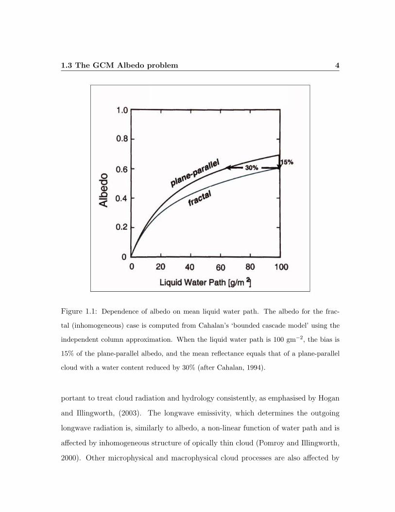
Davies (1992)) have revealed that GCMs would consistently over-estimate albedo
by as much as 15% when using realistic liquid water content (LWC) values. The
cause of this problem is the non-linear dependence of albedo on optical thickness, or
equivalently, on the vertically integrated liquid water content, known as the liquid
water path (LWP). If a cloud exhibits structure over a large range of scales, the
albedo corresponding to the mean LWP (i.e. the plane-parallel albedo) is not the
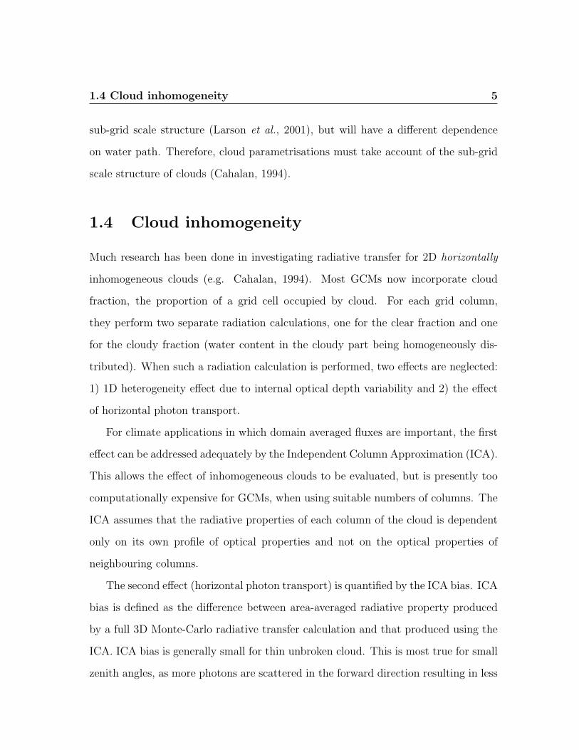
same as the true mean albedo (see figure 1.1).
Cahalan (1994) showed that the albedo of marine stratocumulus can be approxi-
mated well using the PP structure if the optical thickness presented to the radiation
scheme is reduced from the true mean optical thickness by a factor χ(α, σ). Here α
is a parameter linked to the scale of the cloud structure, and σ is the standard devia-
tion of log10(LWP). For a stratocumulus albedo bias of 15%, the calculated reduction
factor was approximately 0.7. The European Centre for Medium-range Weather Fore-
casts (ECMWF) still apply this reduction factor of 0.7 in their GCM for all clouds
(Tiedtke, 1996), even though the calculation was specific to marine stratocumulus.
According to Cahalan (1994) larger albedo biases may occur for other cloud types
although these have smaller global coverage.
As GCMs are starting to carry water content as a prognostic variable, it is im-
1.3 The GCM Albedo problem 4
Figure 1.1: Dependence of albedo on mean liquid water path. The albedo for the frac-
tal (inhomogeneous) case is computed from Cahalan’s ‘bounded cascade model’ using the
independent column approximation. When the liquid water path is 100 gm−2, the bias is
15% of the plane-parallel albedo, and the mean reflectance equals that of a plane-parallel
cloud with a water content reduced by 30% (after Cahalan, 1994).
portant to treat cloud radiation and hydrology consistently, as emphasised by Hogan
and Illingworth, (2003). The longwave emissivity, which determines the outgoing
longwave radiation is, similarly to albedo, a non-linear function of water path and is
affected by inhomogeneous structure of opically thin cloud (Pomroy and Illingworth,
2000). Other microphysical and macrophysical cloud processes are also affected by
1.4 Cloud inhomogeneity 5
sub-grid scale structure (Larson et al., 2001), but will have a different dependence
on water path. Therefore, cloud parametrisations must take account of the sub-grid
scale structure of clouds (Cahalan, 1994).
1.4 Cloud inhomogeneity
Much research has been done in investigating radiative transfer for 2D horizontally
inhomogeneous clouds (e.g. Cahalan, 1994). Most GCMs now incorporate cloud
fraction, the proportion of a grid cell occupied by cloud. For each grid column,
they perform two separate radiation calculations, one for the clear fraction and one
for the cloudy fraction (water content in the cloudy part being homogeneously dis-
tributed). When such a radiation calculation is performed, two effects are neglected:
1) 1D heterogeneity effect due to internal optical depth variability and 2) the effect
of horizontal photon transport.
For climate applications in which domain averaged fluxes are important, the first
effect can be addressed adequately by the Independent Column Approximation (ICA).
This allows the effect of inhomogeneous clouds to be evaluated, but is presently too
computationally expensive for GCMs, when using suitable numbers of columns. The
ICA assumes that the radiative properties of each column of the cloud is dependent
only on its own profile of optical properties and not on the optical properties of
neighbouring columns.
The second effect (horizontal photon transport) is quantified by the ICA bias. ICA
bias is defined as the difference between area-averaged radiative property produced
by a full 3D Monte-Carlo radiative transfer calculation and that produced using the
ICA. ICA bias is generally small for thin unbroken cloud. This is most true for small
zenith angles, as more photons are scattered in the forward direction resulting in less
1.5 Fractal models of stratocumulus 6
horizontal photon transport between columns (Cahalan, 1994). However, in the case
of broken stratocumulus clouds, the ICA bias can be large (up to 30% due to side
illumination, intercloud interaction and shadowing effects) and even the sign of the
bias is uncertain (Di Guiseppe and Tompkins, 2003).
1.5 Fractal models of stratocumulus
Efforts to develop cloud resolving numerical models that resemble cloud observa-
tions more closely are now underway. Such models are required in order to improve
parametrisations used to represent clouds in GCMs. We need to know how the
parametrisations behave and upon what they depend. The closer the model proper-
ties are to true cloud properties, the more realistic the radiative transfer calculations
will be. True observations could be directly used to obtain parameters required
in radiation calculations in some cases; however, these observations are mostly 2D
(e.g. satellite imagery, stationary radar/lidar). Any existing 3D observation tech-
niques such as sweeping radar scanning are limited in resolution and are limited in
experimental value. Alternatively, developing a model which can reproduce cloud pa-
rameters from observations would permit an investigation of the effect of realistically
plausible changes of cloud parameters on radiative transfer.
Fractals are objects, such as clouds, which appear to be extremely irregular and
yet are statistically invariant under a change of scale. Remote sensing observations
show that many clouds possess fractal properties that fit wavenumber power-law
statistics (e.g. Danne et al. (1996), Barker and Davies (1992), Cahalan and Snider
(1989)). Lovejoy (1982) presented evidence that clouds are statistically self-similar
in the horizontal plane from 1000 km down to 1km, and Cahalan and Snider (1989),

1.5 Fractal models of stratocumulus 7
presented supportive findings based on data from the FIRE (First ISCCP1 Regional
Experiment) programme. They showed that vertically integrated liquid water follows
a k−5/3 power-law, where k, the wavenumber, is the reciprocal of the length scale.
An abrupt transition to smoother scaling behaviour occurs at scales less than a few
100 m. According to Davis et al. (1997), this break of scale is due to the mean
photon path length between scattering events being approximately 100 m, and so
below this scale, statistics derived from satellite radiance measurements are affected.
These smaller scales are reported not to have a significant effect on large-scale albedo
(Cahalan and Joseph, 1989).
Cahalan (1994) developed a very simple fractal model, known as the bounded
fractal cascade, to obtain a linear log-log power spectrum of LWC with a spectral
exponent of -5/3. Much has been brought to light from such models, such as the
problem of albedo bias, but due to their unrealistic, inherently ‘square’ geometry, they
are only really appropriate for overcast situations in which the ICA bias is minimal.
The geometry also renders it difficult to introduce realistic vertical structure, which
often varies considerably from cloud-base to top (Di Guiseppe and Tompkins, 2003).
For realistic geometrical structure, we must turn to alternative techniques of gen-
erating fractal structure. One such approach is to specify scale invariance over a
range of scales in Fourier space, and use inverse Fast Fourier Transforms (FFT) to
produce the cloud field in physical space (e.g. Davis et al. (1997), Evans and Wis-
combe (2003), Di Guiseppe and Tompkins (2003), Hogan and Illingworth (1999)).
Incorporating wavenumber spectra into a fractal model is simple, at least when an
isotropic grid spacing is used, and also carries additional properties, thought to be
important e.g. a continuous size distribution and continuous scale invariance over a
wide range of scales.
1The ‘International Satellite Cloud Climatology Project’.
1.6 GCMs and vertical structure of cirrus 8
Barker and Davies (1992) and Evans and Wiscombe (2003) presented stochastic
models with horizontal spectral isotropy for boundary-layer clouds. In both cases,
Fourier-filtering techniques were used to produce a spectral slope of cloud LWC based
on observed values. In their 2D model of cumuloform clouds, Barker and Davies
observed that as they steepened the scaling exponent, the distribution of cloud size
in the field narrowed, the mean area of individual clouds increased, variability across
individual clouds decreased and the albedo decreased. However no specific comment
was made concerning the dependence and variability of parameters with height. This
issue was raised by Cahalan and Joseph (1989). They went part-way to producing
an answer for different boundary layer clouds by using Landsat satellite observations
to calculate their fractal perimeters. Two widely separated thresholds, one for cloud-
base and one for cloud-top, were determined for each cloud scene examined, and the
sensitivity of cloud spatial structure to changes in threshold was investigated. It was
found that the perimeter fractal dimension increased from cloud base to top, which
they suggested was indicative of increased turbulence at cloud top, but only data
from these two levels were presented.
Di Guiseppe and Tompkins (2003) also investigated vertical structure, with an
idealised model of stratocumulus, making use of Fourier transforms to create 2D
cloud fields. Vertical structure was subsequently introduced using a simple turbulence
theory which was applicable to boundary layer clouds.
1.6 GCMs and vertical structure of cirrus
Vertical structure is more likely to be important in cirrus than in stratocumulus. Stra-
tocumulus are typically 200 - 500 m thick whereas cirrus often have a vertical range
greater than 3 km, and frequently characterised by slanted fall streaks (which are de-
1.7 Observations of cirrus 9
scribed in chapter 2). Most cirrus clouds will span several vertical GCM grid boxes,
which typically have vertical resolutions of 0.5 - 0.75 km at cirrus altitudes (Hogan
and Illingworth, 2000). By good fortune, GCMs can go part-way in prescribing verti-
cal structure when changes in the cloud fraction with height are translated by ‘cloud
overlap rules’ into effective horizontal variability of integrated cloud quantities, such
as water path (Di Guiseppe and Tompkins, 2003). However, GCMs usually make
the simplest assumption of maximum overlap between neighbouring cloudy layers
(Hogan and Illingworth, 2000), resulting in moderately few possible cloud configu-
rations (Pincus et al., 2002). In nature, the same sized domains have substantially
more horizontal variability and complicated vertical structure (e.g. Hogan and Illing-
worth, 2000). GCMs will therefore have to add some kind of representation of cloud
inhomogeneity and its vertical correlation in future.
1.7 Observations of cirrus
Millimetre-wave radar is currently the sole remote sensing instrument that allows
high-resolution observations of the vertical structure and properties of clouds in all
types of conditions. Hogan and Illingworth (1999) simulated a 2D cirrus cloud field,
using 1D spectral information obtained from radar observations at a specified height.
They generated fields by performing the inverse Fourier transform of a 2D array
containing ‘wave amplitudes consistent with the energy at the various scales indicated
by the 1D spectrum’. The spectral slope of their field was -2.16. Like all models
mentioned here so far, their 2D fields were spectrally isotropic. Real cirrus clouds
with fall streaks are, however, spectrally anisotropic in the horizontal, as fall streaks
tend to be aligned parallel to the vertical wind shear. Previous models of cirrus
containing fall streaks are limited. Danne et al. (1996) modelled the fall streaks of
1.8 Development of a 3D fractal cirrus model 10
cirrus as a series of idealised, sinusoidal ‘cloud cells’ in the x− z plane, assuming the
pattern to be constant in the y direction. The model served a purpose of validating
a particular theory rather than advancing cirrus research. The spectra plotted in
figure 4 of their paper suggest spectral slopes of -3.5 and -2.4. They acknowledged
that further aspects should be accounted for in 2- or 3- dimensions, such as the
tilting structure of the fall streaks due to vertical wind shear, or temporal and spatial
changes of the wind direction. Whilst it is not possible to model the spatial changes
in the wind profile using the Fourier technique, implementing the tilting of the fall
streaks should be fairly straight forward.
1.8 Development of a 3D fractal cirrus model
No attempt has yet been made to create a 3D stochastic model of cirrus, and as
of yet no suitable observations in 3D exist. In this study we develop a 3D fractal
cirrus cloud model, which has realistic horizontal and vertical structure based on 2D
(height-time) radar observations. The model will produce a 3D field of IWC which can
be presented to radiation schemes in order to assess the effect of the inhomogeneity
and characterise the vertical structure of cirrus on radiative transfer. In addition,
the model could be used as a tool in the interpretation of cirrus measurements in a
2D plane, for example, plan-view images from satellite or vertical cross-sections from
ground based or spaceborne (following the launch of CloudSat in 2005 (Stephens et al.,
2002)) radar. Implemented in our model are the new aspects of three-dimensionally
resolved fall streak geometry for any wind shear situation, anisotropic horizontal
scaling and variation of power-law slope with height. The power-law for each height
is wavenumber-dependent, with a cut-off applied at the wavenumber corresponding
to the largest observed scale length. It is also possible to include a change in slope at
1.8 Development of a 3D fractal cirrus model 11
a characteristic wavenumber. The IWC for each height is scaled such that the mean
IWC and standard deviation of ln(IWC) are matched to the radar observations.
The grid resolution is equal for the two horizontal dimensions but is greater in
the vertical. The adaptations of the Fourier method made to achieve this anisotropic
spacing are specific to this study and different to that considered (but not applied
to a model) by Evans and Wiscombe (2003). The advantage of our method is that
it can be understood from physical arguments (concerning spectral energy density)
whereas the suggested approach of Evans and Wiscombe, although it undoubtedly
gives adequate results, is not linked to a physical process or reason.
Assumptions of our cloud model are:
1. A constant effective radius for ice crystals. This will isolate the effects of IWC
variations on cloud radiative properties. A variable effective radius could be
introduced by exploiting its dependence on IWC and temperature. This is a
possibility for further work.
2. IWC follows a log-normal probability distribution function (PDF) defined for
each height. This appears to be a good fit for some observations, but not all
(Hogan and Illingworth, 2003). However, the model is not limited to this PDF.
The method of Evans and Wiscombe (which was to use a look-up table to
transform a gaussian field of ln(IWC) to one having the observed PDF) could
quite easily be applied.
3. The generating level, the height at which cirrus formation begins, is constant
throughout the domain of the model. This is a limitation of the Fourier tech-
nique. There are likely to be small departures from this in reality, but these are
assumed to be insignificant.
1.9 Outline 12
The Edwards-Slingo 1D radiative transfer code (Edwards and Slingo, 1996) is
employed to assess the effect of different scenarios (e.g. different wind shears) on
the long-wave and short-wave radiative fluxes. For this we assume the ICA. The
ICA is a strong assumption, justified by Cahalan (1994) for stratocumulus mesoscale
domain-averaged fluxes, by the finding that flux increase and decrease due to hor-
izontal transport tend to approximately cancel each other over the total area. To
investigate the validity of the ICA for cirrus it would be necessary to perform a full
3D radiative transfer calculation. It would be interesting to observe how horizontal
photon transport is affected by fall streak orientation, but the required code is not
yet ready for use. If significant results are obtained from the full-3D calculation, they
will be reported elsewhere.
1.9 Outline
The next section provides a description of cirrus with particular reference to the
fall streak geometry. Sections 3 and 4 describe the analysis of the radar data and
the generation of the 3D fractal cirrus model respectively. Together they comprise
the method. The radiative transfer code, radiation experiments and the results are
described in section 5 and finally the conclusions are drawn in section 6.
Chapter 2
Cirrus cloud geometry
Here we give a brief description of cirrus, for the purpose of introducing some of the
concepts and terminology which will feature in later sections.
2.1 Definition of cirrus
Clouds are officially classified by morphology. The internationally agreed definition
of cirrus clouds, given by the World Meteorological Organisation (WMO), is:
Cirrus (Ci): Detached clouds in the form of white, delicate filaments
or white or mostly white patches or narrow bands. These clouds have a
fibrous (hair-like) appearance, or a silky sheen or both.
Cirrocumulus (Cc): Thin, white patch, sheet or layer of cloud without
shading, composed of very small elements in the form of grains, ripples,
etc., merged or separate, and more or less regularly arranged; most of the
elements have an apparent width of less than one degree.
Cirrostratus (Cs): Transparent, whitish cloud veil of fibrous (hair-like)
13
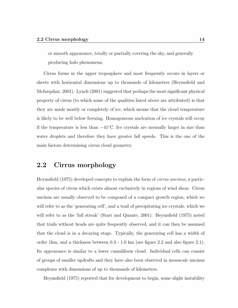
2.2 Cirrus morphology 14
or smooth appearance, totally or partially covering the sky, and generally
producing halo phenomena.
Cirrus forms in the upper troposphere and most frequently occurs in layers or
sheets with horizontal dimensions up to thousands of kilometres (Heymsfield and
Mcfarquhar, 2001). Lynch (2001) suggested that perhaps the most significant physical
property of cirrus (to which some of the qualities listed above are attributed) is that
they are made mostly or completely of ice, which means that the cloud temperature
is likely to be well below freezing. Homogeneous nucleation of ice crystals will occur
if the temperature is less than −41◦C. Ice crystals are normally larger in size than
water droplets and therefore they have greater fall speeds. This is the one of the
main factors determining cirrus cloud geometry.
2.2 Cirrus morphology
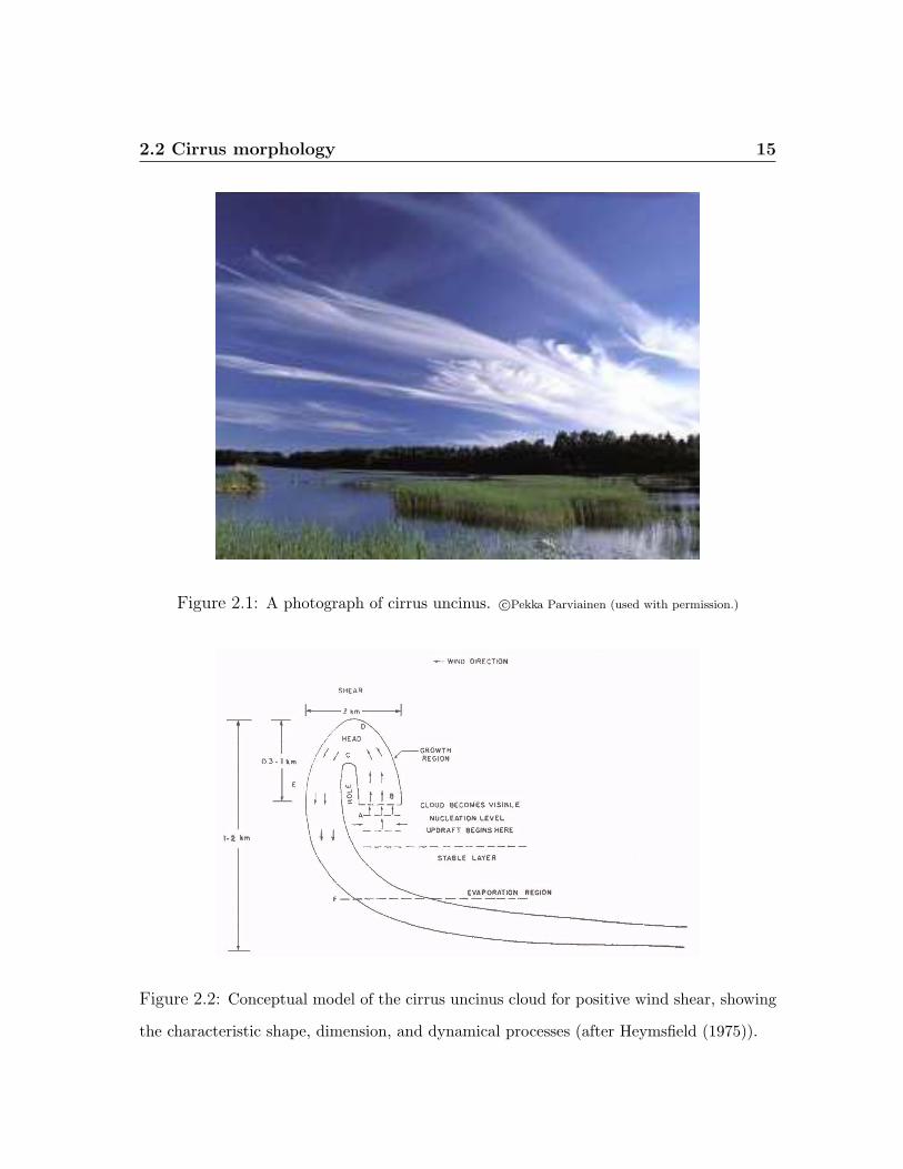
Heymsfield (1975) developed concepts to explain the form of cirrus uncinus, a partic-
ular species of cirrus which exists almost exclusively in regions of wind shear. Cirrus
uncinus are usually observed to be composed of a compact growth region, which we
will refer to as the ‘generating cell’, and a trail of precipitating ice crystals, which we
will refer to as the ‘fall streak’ (Starr and Quante, 2001). Heymsfield (1975) noted
that trails without heads are quite frequently observed, and it can then be assumed
that the cloud is in a decaying stage. Typically, the generating cell has a width of
order 1km, and a thickness between 0.3 - 1.0 km (see figure 2.2 and also figure 2.1).
Its appearance is similar to a lower cumuliform cloud. Individual cells can consist
of groups of smaller updrafts and they have also been observed in mesoscale uncinus
complexes with dimensions of up to thousands of kilometres.
Heymsfield (1975) reported that for development to begin, some slight instability
2.2 Cirrus morphology 15
Figure 2.1: A photograph of cirrus uncinus. c©Pekka Parviainen (used with permission.)
Figure 2.2: Conceptual model of the cirrus uncinus cloud for positive wind shear, showing
the characteristic shape, dimension, and dynamical processes (after Heymsfield (1975)).
2.2 Cirrus morphology 16
is necessary in order to initiate convection and updrafts. In addition, the relative hu-
midity must be high enough for nucleation to occur (figure 2.2 level A). Once formed,
the crystals grow rapidly and continue moving with the updraft (figure 2.2 level B).
As the crystals grow, their fall speed will increase and at some point they will start
to fall down through the updraft and become part of the fall streak.
Cirrus fall streaks may curve irregularly or slant sometimes with a comma shape
as a result of the changes in horizontal wind velocity with height and variations in
fall speed (Heymsfield and McFarquhar, 2001). The fall streak pattern as a whole
moves with the same speed as the generating cell, which itself remains at about the
same height and advects with the horizontal wind velocity at that height (Marshall,
1953). Note that the trajectory of an ice crystal is not the same as the fall streak
structure. The former is the trace in time of an individual crystal (which will have
smaller horizontal velocity than that of the generating cell when there is positive wind
shear), whereas the latter can be thought of as a snap shot of the whole fall streak
taken at one particular moment.
Marshall (1953) studied the characteristic mares tail pattern of falling snow and
came to the conclusion that the snow is continuously generated in generating ele-
ments. In a case of nearly constant wind shear, the mares tails, or fall streaks, were
parabolic, and before reaching the ground became almost horizontal. In appendix A
it is shown how the fall streak structure can be determined for arbitrary wind shear,
based on the findings of Marshall (1953).
Chapter 3
Analysis of Observations
This section describes how radar data on which the model is based is analysed. The
radar data are used to characterise all the relevant properties of cirrus that we wish
to capture in our model. The characteristics considered are spectral properties and
their height dependence, the mean and spread of IWC at each height, and the fall
streak structure. The simulations will use a 128×128×32 point grid. The horizontal
dimensions of the domain, x and y, are both chosen to be 200 km, whilst the vertical
dimension, z, is 5 km. This gives a resolution of 1562.5 m in the horizontal and
156.25 m in the vertical. These dimensions and resolutions apply to all figures, in
this section and the next, unless otherwise stated.
3.1 The Galileo Radar
The observations from which the cloud model statistics are derived are obtained from
Galileo, a 94 GHz, 0.45 m diameter cloud radar located at Chilbolton in the South of
the UK. The radar is vertically pointing and operates with a pulse width of 0.5 µs.
The radar reflectivity factor Z is averaged over 30 second periods and is recorded for
17
3.2 Using time as a horizontal dimension 18
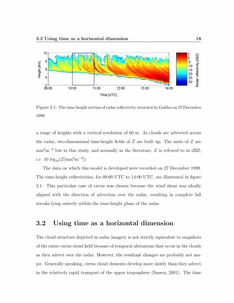
Figure 3.1: The time-height section of radar reflectivity recorded by Galileo on 27 December
1999.
a range of heights with a vertical resolution of 60 m. As clouds are advected across
the radar, two-dimensional time-height fields of Z are built up. The units of Z are
mm6m−3 but in this study, and normally in the literature, Z is referred to in dBZ,
i.e. 10 log10(Z[mm6m−3]).
The data on which this model is developed were recorded on 27 December 1999.
The time-height reflectivities, for 09:00 UTC to 14:00 UTC, are illustrated in figure
3.1. This particular case of cirrus was chosen because the wind shear was ideally
aligned with the direction of advection over the radar, resulting in complete fall
streaks lying entirely within the time-height plane of the radar.
3.2 Using time as a horizontal dimension
The cloud structure depicted in radar imagery is not strictly equivalent to snapshots
of the entire cirrus cloud field because of temporal alterations that occur in the clouds
as they advect over the radar. However, the resultant changes are probably not ma-
jor. Generally speaking, cirrus cloud elements develop more slowly than they advect
in the relatively rapid transport of the upper troposphere (Sassen, 2001). The time
3.2 Using time as a horizontal dimension 19
dimension is converted to horizontal distance using the assumption that the cloud
moves with speed equal to the wind speed at the generating level (Marshall, 1953).
Evans et al. (2001) also used this approach. The height of the generating level can
be directly but subjectively determined if generating cells can be seen in the Z cross-
section. Otherwise, an informed guess can be made from the temperature profile.
Temperature soundings of cirrus generating cells by Heymsfield (1975) indicated sta-
ble layers above and below the cell, whilst the cell itself was in a region with a dry
adiabatic lapse rate. Typically generating cells are about 1 km thick (see figure 2.2),
so if the temperature profile were unavailable, a crude approximation of 1 km below
the cloud top for the generating level height could be made. The estimation can be
refined in the simulation phase, by comparing the model’s fall streak pattern with
the observed pattern (see section 4.8.1).
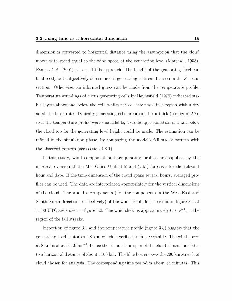
In this study, wind component and temperature profiles are supplied by the
mesoscale version of the Met Office Unified Model (UM) forecasts for the relevant
hour and date. If the time dimension of the cloud spans several hours, averaged pro-
files can be used. The data are interpolated appropriately for the vertical dimensions
of the cloud. The u and v components (i.e. the components in the West-East and
South-North directions respectively) of the wind profile for the cloud in figure 3.1 at
11:00 UTC are shown in figure 3.2. The wind shear is approximately 0.04 s−1, in the
region of the fall streaks.
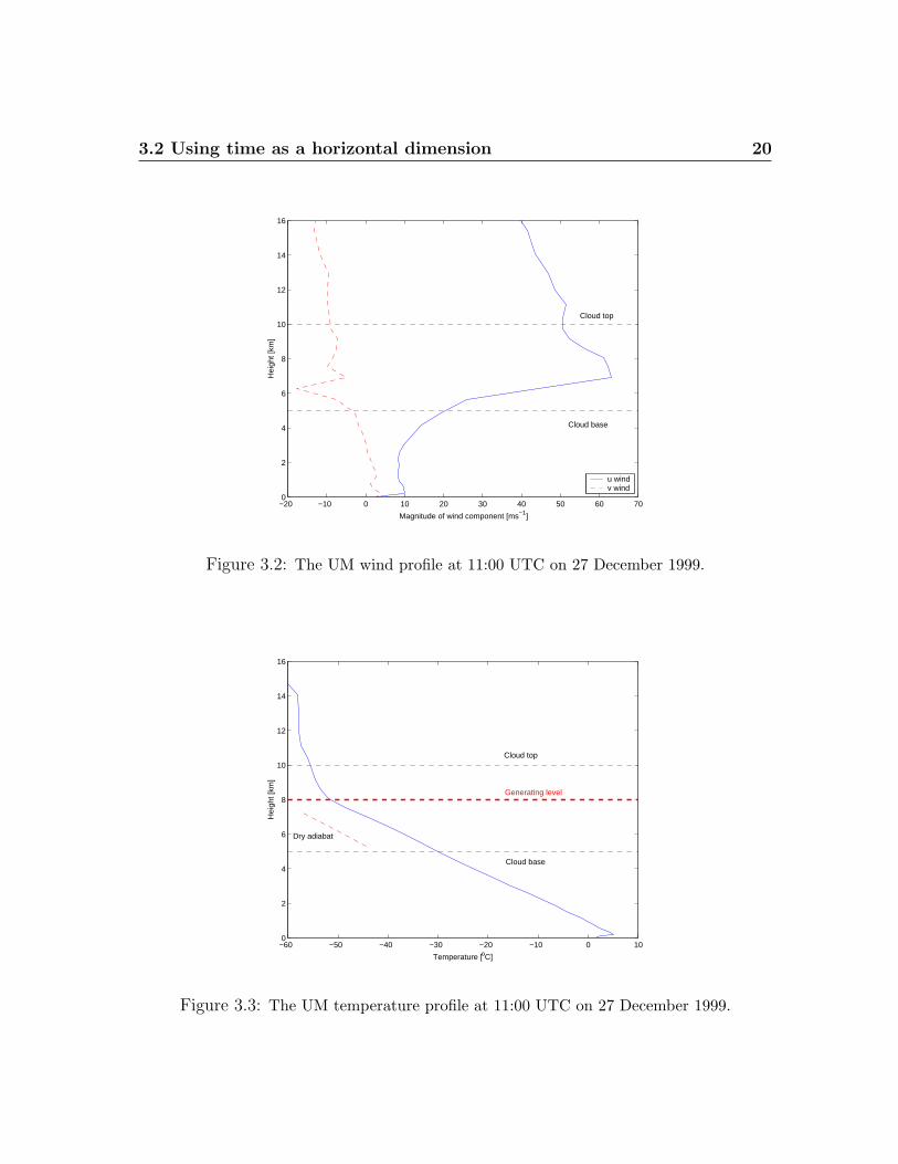
Inspection of figure 3.1 and the temperature profile (figure 3.3) suggest that the
generating level is at about 8 km, which is verified to be acceptable. The wind speed
at 8 km is about 61.9 ms−1, hence the 5-hour time span of the cloud shown translates
to a horizontal distance of about 1100 km. The blue box encases the 200 km stretch of
cloud chosen for analysis. The corresponding time period is about 54 minutes. This
3.2 Using time as a horizontal dimension 20
−20 −10 0 10 20 30 40 50 60 700
2
4
6
8
10
12
14
16
Magnitude of wind component [ms−1]
Hei
ght [
km]
Cloud base
Cloud top
u windv wind
Figure 3.2: The UM wind profile at 11:00 UTC on 27 December 1999.
−60 −50 −40 −30 −20 −10 0 100
2
4
6
8
10
12
14
16
Temperature [oC]
Hei
ght [
km]
Dry adiabat
Cloud top
Cloud base
Generating level
Figure 3.3: The UM temperature profile at 11:00 UTC on 27 December 1999.
3.3 Z-IWC relation 21
particular section was chosen because the cloud base is relatively flat. The horizontal
domain size of 200 km encompasses the largest horizontal scale of variation (which
we will see later is about 60 km).
3.3 Z-IWC relation
In order to compare the output of the model with those from other models, and
also to be able to run a radiation scheme over the cloud, the cloud field should be
defined using universal physical units (LWC or IWC), rather than units such as radar
reflectivity, which are specific to the observation method used.
A 2D time-height field of Ice Water Content (IWC) is computed from the radar
reflectivity factor (Z), using the following empirical Z-IWC relationship, derived from
the data of Liu and Illingworth (2000):
log10(IWC [gm−3]) = 0.0868Z [dBZ]− 0.02106T [◦C]− 1.259, (3.1)
where the temperature, T , is obtained from the UM profiles. Note that this relation-
ship is specific to radars operating at a frequency of 94 GHz and is appropriate only
for ice clouds.
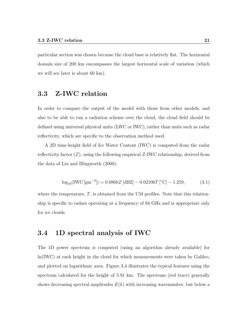
3.4 1D spectral analysis of IWC
The 1D power spectrum is computed (using an algorithm already available) for
ln(IWC) at each height in the cloud for which measurements were taken by Galileo,
and plotted on logarithmic axes. Figure 3.4 illustrates the typical features using the
spectrum calculated for the height of 5.91 km. The spectrum (red trace) generally
shows decreasing spectral amplitudes E(k) with increasing wavenumber, but below a
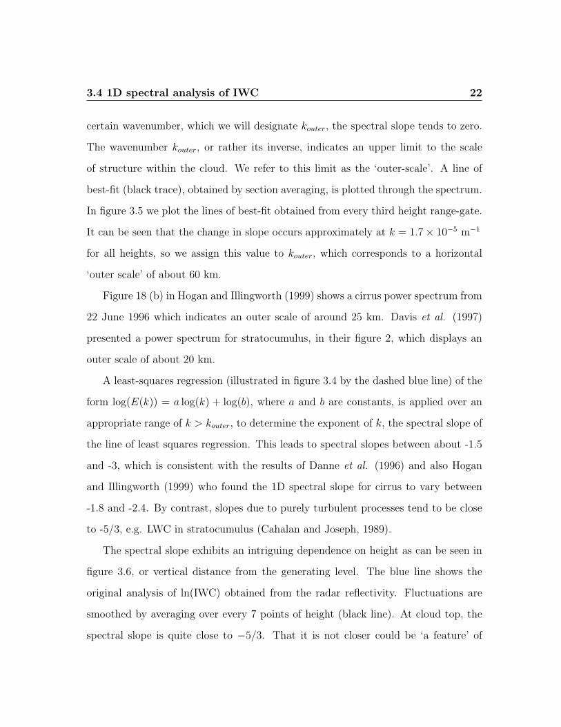
3.4 1D spectral analysis of IWC 22
certain wavenumber, which we will designate kouter, the spectral slope tends to zero.
The wavenumber kouter, or rather its inverse, indicates an upper limit to the scale
of structure within the cloud. We refer to this limit as the ‘outer-scale’. A line of
best-fit (black trace), obtained by section averaging, is plotted through the spectrum.
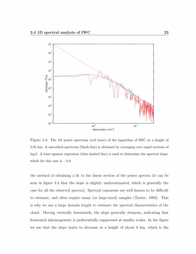
In figure 3.5 we plot the lines of best-fit obtained from every third height range-gate.
It can be seen that the change in slope occurs approximately at k = 1.7× 10⁻⁵ m−1
for all heights, so we assign this value to kouter, which corresponds to a horizontal
‘outer scale’ of about 60 km.
Figure 18 (b) in Hogan and Illingworth (1999) shows a cirrus power spectrum from
22 June 1996 which indicates an outer scale of around 25 km. Davis et al. (1997)
presented a power spectrum for stratocumulus, in their figure 2, which displays an
outer scale of about 20 km.
A least-squares regression (illustrated in figure 3.4 by the dashed blue line) of the
form log(E(k)) = a log(k) + log(b), where a and b are constants, is applied over an
appropriate range of k > kouter, to determine the exponent of k, the spectral slope of
the line of least squares regression. This leads to spectral slopes between about -1.5
and -3, which is consistent with the results of Danne et al. (1996) and also Hogan
and Illingworth (1999) who found the 1D spectral slope for cirrus to vary between
-1.8 and -2.4. By contrast, slopes due to purely turbulent processes tend to be close
to -5/3, e.g. LWC in stratocumulus (Cahalan and Joseph, 1989).
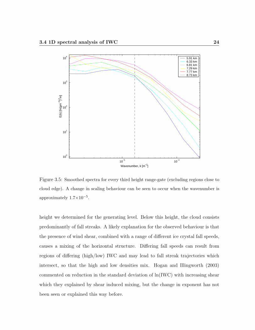
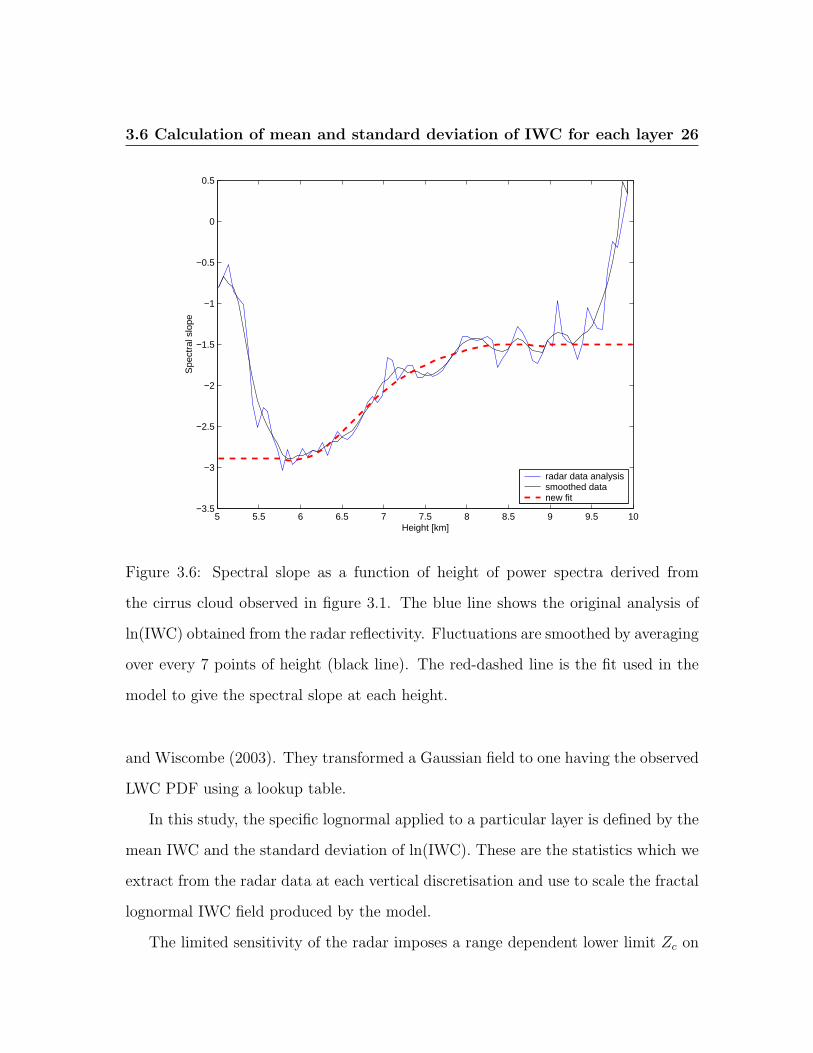
The spectral slope exhibits an intriguing dependence on height as can be seen in
figure 3.6, or vertical distance from the generating level. The blue line shows the
original analysis of ln(IWC) obtained from the radar reflectivity. Fluctuations are
smoothed by averaging over every 7 points of height (black line). At cloud top, the
spectral slope is quite close to −5/3. That it is not closer could be ‘a feature’ of
3.4 1D spectral analysis of IWC 23
10−5
10−4
10−2
10−1
100
101
102
103
104
105
106
107
Wavenumber, k [m−1]
E(k
) [ln
(gm
−3 )2 m
]
Figure 3.4: The 1D power spectrum (red trace) of the logarithm of IWC at a height of
5.91 km. A smoothed spectrum (black line) is obtained by averaging over equal sections of
log k. A least squares regression (blue dashed line) is used to determine the spectral slope,
which for this case is −2.9.
the method of obtaining a fit to the linear section of the power spectra (it can be
seen in figure 3.4 that the slope is slightly underestimated, which is generally the
case for all the observed spectra). Spectral exponents are well known to be difficult
to estimate, and often require many (or large-sized) samples (Tessier, 1993). This
is why we use a large domain length to estimate the spectral characteristics of the
cloud. Moving vertically downwards, the slope generally steepens, indicating that
horizontal inhomogeneity is preferentially suppressed at smaller scales. In the figure
we see that the slope starts to decrease at a height of about 8 km, which is the
3.4 1D spectral analysis of IWC 24
10−5
10−4
100
101
102
103
104
Wavenumber, k [m−1]
E(k
) [ln
(gm
−3 )2 m
]5.91 km6.33 km6.81 km7.29 km7.77 km8.73 km
Figure 3.5: Smoothed spectra for every third height range-gate (excluding regions close to
cloud edge). A change in scaling behaviour can be seen to occur when the wavenumber is
approximately 1.7×10⁻⁵.
height we determined for the generating level. Below this height, the cloud consists
predominantly of fall streaks. A likely explanation for the observed behaviour is that
the presence of wind shear, combined with a range of different ice crystal fall speeds,
causes a mixing of the horizontal structure. Differing fall speeds can result from
regions of differing (high/low) IWC and may lead to fall streak trajectories which
intersect, so that the high and low densities mix. Hogan and Illingworth (2003)
commented on reduction in the standard deviation of ln(IWC) with increasing shear
which they explained by shear induced mixing, but the change in exponent has not
been seen or explained this way before.
3.5 Removal of white noise 25
3.5 Removal of white noise
Towards the cloud-top and cloud-base, the slope appears to flatten towards zero. This
is a consequence of the system noise becoming comparable or greater than the radar
reflectivity from the very low ice crystal concentrations in these regions. This led to
gaps in the data which were dealt with by removing them and compressing the data.
Consequently, towards the cloud base and cloud top, the spectral slope is shallower
than we expected it to be. This effect needs to be eliminated from the model as it
has no physical significance. We assume that the slope remains at its minimum value
towards the cloud base, and tails off at cloud top (to around −3/2) as indicated in
figure 3.6 by the dashed red line.
3.6 Calculation of mean and standard deviation of
IWC for each layer
In order to estimate the true statistics of the cloud, the underlying probability density
function (PDF) of IWC needs to be modelled. In this study we assume a lognormal
distribution for IWC. The use of a lognormal PDF for water content has been sug-
gested and used by Cahalan et al. (1994), Evans and Wiscombe (2003), and Hogan
and Illingworth (2003). Cahalan et al. (1994) graphed the one-point PDF of Liquid
Water path for stratocumulus and overplotted a lognormal with the same mean and
variance, finding it to be a good fit. Evans and Wiscombe (2003) also stated that the
PDF of LWC is usually close to being lognormal. Research by Hogan and Illingworth
(2003) on ice clouds has shown that a lognormal PDF is a good fit for many IWC
observations. The PDF for IWC is a flexible feature of this model and so a different
function, even the exact PDF could be used. This was the approach taken by Evans
3.6 Calculation of mean and standard deviation of IWC for each layer 26
5 5.5 6 6.5 7 7.5 8 8.5 9 9.5 10−3.5
−3
−2.5
−2
−1.5
−1
−0.5
0
0.5
Height [km]
Spe
ctra
l slo
pe
radar data analysissmoothed datanew fit
Figure 3.6: Spectral slope as a function of height of power spectra derived from
the cirrus cloud observed in figure 3.1. The blue line shows the original analysis of
ln(IWC) obtained from the radar reflectivity. Fluctuations are smoothed by averaging
over every 7 points of height (black line). The red-dashed line is the fit used in the
model to give the spectral slope at each height.
and Wiscombe (2003). They transformed a Gaussian field to one having the observed
LWC PDF using a lookup table.
In this study, the specific lognormal applied to a particular layer is defined by the
mean IWC and the standard deviation of ln(IWC). These are the statistics which we
extract from the radar data at each vertical discretisation and use to scale the fractal
lognormal IWC field produced by the model.
The limited sensitivity of the radar imposes a range dependent lower limit Zc on
3.6 Calculation of mean and standard deviation of IWC for each layer 27
the radar reflectivity which is registered which, for Galileo, varies from around -50
dBZ at 1 km to -30 dBZ at 10 km. The limited sensitivity results in missing data
values where the true IWC corresponds to Z < Zc . In this study, we assume that
if Z < Zc, we have clear sky. However, we still need to take account of the missing
values in order to define the most correct lognormal PDF. Two approaches to this
problem are taken. The most simplistic approach assumes all Z < Zc at a specific
height take an identical value, for example, that corresponding to IWC(Zc)/2. A
more sophisticated approach is based on the assumption that the underlying distri-
bution of Z in logarithmic units, dBZ, is a Normal, with a mean Zm and standard
deviation σz. The parameters Zm and σz can be estimated if we know the fraction f
of the underlying PDF for which a valid value has been recorded. The details of this
approach can be found in appendix B. The second approach is used for estimating the
standard deviation of ln(IWC). However, when used to estimate the mean IWC, this
approach occasionally yielded a mean IWC outside of the expected range (where the
minimum expected mean is obtained by replacing the missing values with 0 and the
maximum expected mean is obtained by replacing the missing values with IWC(Zc)),
indicating that the PDF of Z, or of ln(IWC), departs from a Normal distribution
when the IWC is low. The first approach was therefore used in preference.
Chapter 4
Generation of the 3D model
This section outlines how the 3D fractal cloud field of IWC is generated using the
radar analysis. The principle is that, for a particular height, a 1D Fourier analysis
of the data yields a power spectrum with information about the structure at various
scales at that same height. Then this information is used to simulate a 3D power
spectrum. An inverse 3D FFT is applied to produce a 3D fractal with the same 1D
power spectral properties as the radar data (if a power spectrum is taken across it).
The 3D model is partly based on adaptations from an existing but much sim-
pler 2D fractal ‘Fourier’ model for cirrus cloud fields. The 2D model uses equal grid
spacing in the x and y directions and produces a spectrally isotropic square field
with fractal characteristics and zero mean. Each component of the Fourier matrix
is a random complex number with a Gaussian distribution and a mean amplitude
proportional to the square-root of the mean spectral energy. The spatial field is
obtained by performing the inverse Fourier transform of the Fourier matrix and se-
lecting the real part. Unique to the 3D model are the manipulations of the spectra
and simulation of the correct vertical structure.
28
4.1 The 3D wavenumber array 29
4.1 The 3D wavenumber array
We require a 3D fractal field, f(x, y, z), consisting of Nx × Ny × Nz points, with
grid spacing ∆x, ∆y and ∆z in the x, y and z directions respectively. We begin
by creating the 3D wavenumber array k, which has the same dimensions as the
fractal field. The maximum wave number in the x-direction is max(kx) = 12∆x
. This
corresponds to a wavelength of twice the grid spacing in the x-direction. Known
as the Nyquist frequency, it is the highest frequency which can be resolved by the
grid. The same applies to maximum wavenumbers in the y- and z-directions. The
wavenumber vector in the x-direction ranges from −max(kx) to max(kx) with spacing
∆kx = 2 max(kx)/Nx, and similarly for y and z, however the order of the elements
must be changed in order to perform the Fourier transform correctly (Press, 1992).
The full 3D array is created from the 1D components using k =√
k2x + k2
y + k2z . A
mean spectral energy density can then be calculated by applying a power-law. The
domain in k-space is very non-cubic because ∆z ¿ ∆x, so max(kz) À max(kx). The
consequences of this are considered in the next section.
4.2 Calculating the 3D mean spectral energy den-
sity
As a starting point we wish to simulate a spectrally isotropic three-dimensional
cloud field using a one-dimensional energy spectrum obtained from radar observa-
tions (anisotropy will be introduced later). This can be thought of as the assumption
that the cloud is generated by turbulent motion at the cloud top and possesses a
spectral slope of near −5/3 in all three orthogonal directions. But how realistic is
this assumption? Orographically or gravity wave driven cirrus have distinct wave-like
4.2 Calculating the 3D mean spectral energy density 30
structures at cloud top, for example. In the scope of this work such complexities are
neglected.
The one-dimensional energy spectrum is of the form
E1(k) = E1kµ, (4.1)
where k is the wavenumber, E1 is the 1D spectral energy density, E1 is a constant
related to the y-axis intercept on a log-log E(k) plot, and µ is a constant equal to
the gradient of the log-log E(k) plot.
Let us firstly consider the case for isotropic grid spacing (∆x = ∆y = ∆z). The
continuous 3D spectral energy density, E3, may then be defined in terms of k, using
the constraint that, at a particular wavenumber, E1 is equal to the integral of E3
over all directions for the same wavenumber:
E1(k) =∫ φ=2π
φ=0
∫ θ=π
θ=0E3(k)k2 sin θ dθ dφ, (4.2)
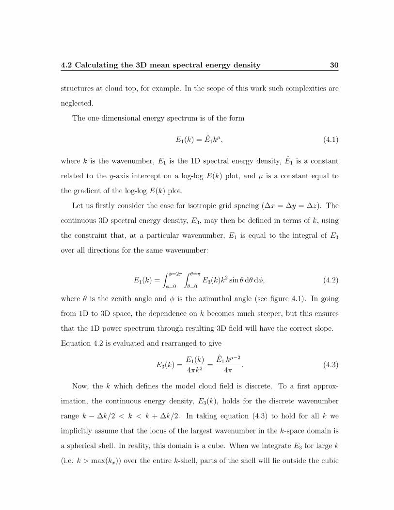
where θ is the zenith angle and φ is the azimuthal angle (see figure 4.1). In going
from 1D to 3D space, the dependence on k becomes much steeper, but this ensures
that the 1D power spectrum through resulting 3D field will have the correct slope.
Equation 4.2 is evaluated and rearranged to give
E3(k) =E1(k)
4πk2=
E1 kµ−2
4π. (4.3)
Now, the k which defines the model cloud field is discrete. To a first approx-
imation, the continuous energy density, E3(k), holds for the discrete wavenumber
range k − ∆k/2 < k < k + ∆k/2. In taking equation (4.3) to hold for all k we
implicitly assume that the locus of the largest wavenumber in the k-space domain is
a spherical shell. In reality, this domain is a cube. When we integrate E3 for large k
(i.e. k > max(kx)) over the entire k-shell, parts of the shell will lie outside the cubic
4.2 Calculating the 3D mean spectral energy density 31
θ
φ
k
r
max(kx)
max(kx)
ky
kx
kz
0
0
Figure 4.1: The geometry employed in k-space. Here θ is the zenith angle and φ is the
azimuth. We define r to be the horizontal component of k when the k-vector just contacts
the boundary of the domain. The dashed line marks the upper limit of φ at π/4, which is
applied when using anisotropic grid spacing.
k-space domain. So, E3 is larger than it should be. This applies to large k only and
here is assumed not to have a significant effect.
If, however, the grid spacing is not isotropic, i.e. ∆x = ∆y À ∆z, equation
(4.3) should no longer be applied to all k. This is because ∆kx (= ∆ky) and ∆kz are
no longer equal. This anisotropy affects both ends of the wavenumber range. It is
important to consider the effect of the inequality ∆kx 6= ∆kz for small k, and the
inequality max(kx) 6= max(kz) for large k. Let us firstly consider the upper range of
k, confined by k > max(kx).
4.2 Calculating the 3D mean spectral energy density 32
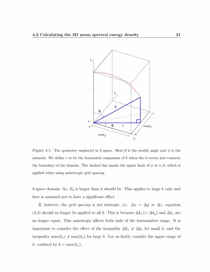
Figure 4.2: Cross-sections in the kx-kz plane at ky=0.. The plotted range of kx is−max(kx)
to + max(kx), while the range of kz is −max(kz)/2 to + max(kz)/2. The grid points have
a large separation, ∆kz, in the kz direction, but in the kx direction they are so closely
spaced that they have merged into (blue) solid lines (a): Intersection of k-shells with the
kx-kz plane. Complete shells exist only when k < max(kx). (b): Intersection of the shells
k = max(kx) (black), k = ∆kz (green) and k = ∆kz/2 (red) with the kx-kz plane.
When k > max(kx), significant portions of the k-shell fall outside of k-space
domain (see figure 4.2). To obtain the ‘correct’ spectral energy density relation
equation for this range of k, we therefore need to change the limits on the integral
over θ in equation (4.2). This analysis ensures that vertical power spectra of the
simulated fractal have the correct spectral slope for scales smaller than ∆x.
4.2 Calculating the 3D mean spectral energy density 33
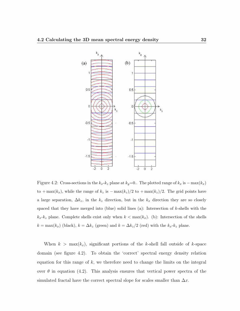
Figure 4.3: Schematic illustrating the different regimes of the 3D power spectrum. The
spectral slope in region (i) remains unchanged. In region (ii) we apply the new equa-
tion (4.8). This reverts back to give the spectral slope in (i) at boundary (1) so a boundary
condition does not have to be determined. In region (iii) we apply the 2D inner spectral
slope and a constant of proportionality, A, is required to satisfy continuity at boundary (2).
In region (iv) we apply the 2D outer spectral slope and a second constant of proportionality,
B, is required to meet the boundary conditions at (3).
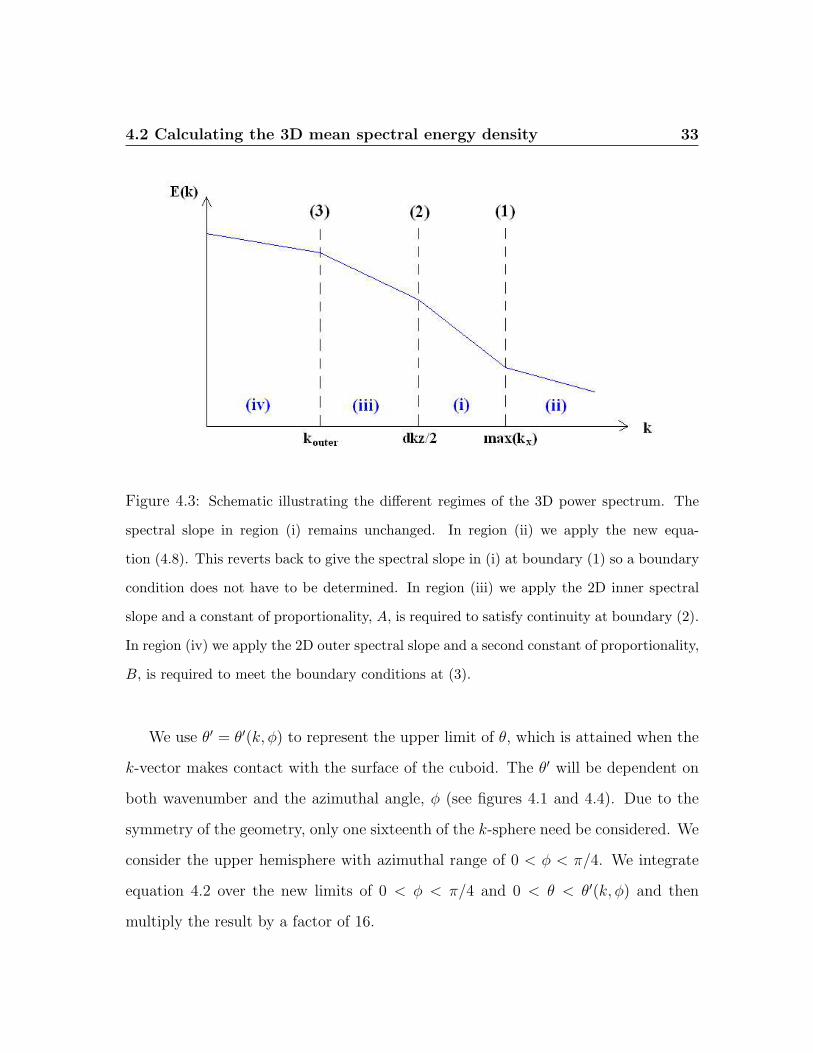
We use θ′ = θ′(k, φ) to represent the upper limit of θ, which is attained when the
k-vector makes contact with the surface of the cuboid. The θ′ will be dependent on
both wavenumber and the azimuthal angle, φ (see figures 4.1 and 4.4). Due to the
symmetry of the geometry, only one sixteenth of the k-sphere need be considered. We
consider the upper hemisphere with azimuthal range of 0 < φ < π/4. We integrate
equation 4.2 over the new limits of 0 < φ < π/4 and 0 < θ < θ′(k, φ) and then
multiply the result by a factor of 16.

4.2 Calculating the 3D mean spectral energy density 34
Figure 4.4: The θ dependence of the integration surface. Diagram (a) illustrates the k-shell
within the domain of integration when k < max(kx), in (b) is the relevant shell shape for
max(kx) < k <√
2max(kx), and (c) applies to all k >√
2max(kx).
E1(k) = 16∫ π/4
0
∫ θ′
0E3(k)k2 sin θ dθ dφ (4.4)
= 16k2E3
∫ π/4
0
(1− cos θ′
)dφ. (4.5)
Now, we can calculate cos θ′ using the geometry shown in figure 4.1:
cos θ′ =
√k2 − r2
k,
where r = max(kx)/ cos φ. Substituting for r, we insert this relation into equation
(4.4) and obtain
E1(k) = 16k2E3
∫ π/4
0
(1−
√1− (max(kx)/k cos φ)2
)dφ. (4.6)
Rearranging (4.6), we find the 3D spectral energy density as a function of the 1D
4.2 Calculating the 3D mean spectral energy density 35
spectral energy density,
E3(k) =E1(k)
16k2∫ π/40
(1−
√1− (max(kx)/k cos φ)2
)dφ
(4.7)
=E1k
µ−2
4π
1
1− 4π
∫ π/40
√1− (max(kx)/k cos φ)2dφ
. (4.8)
The 3D spectral energy density is now defined as the product of the isotropic
domain spectral energy and a new factor which is dependent on φ and on the ratio
of max(kx) to k. The integral in the denominator of equation 4.7 is physically the
surface area of the k-shell inside the k-domain. No analytical solution to this integral
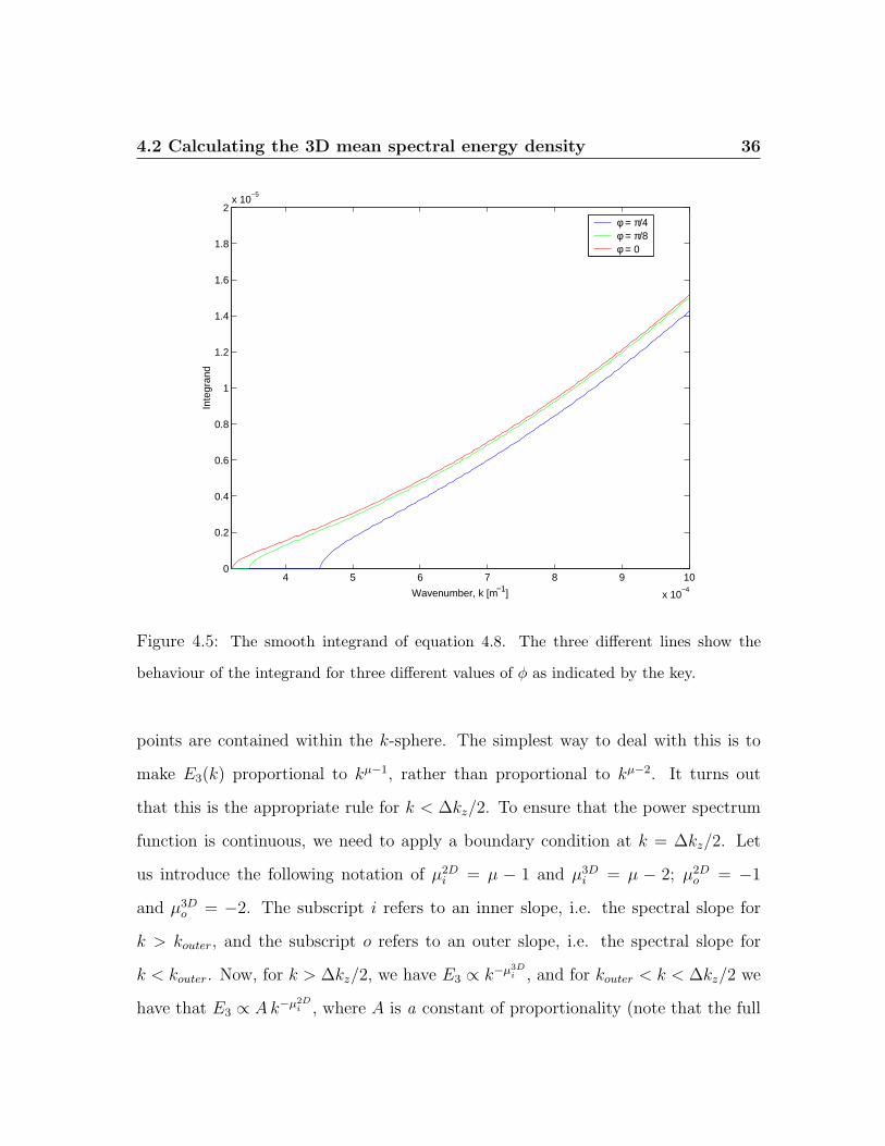
has yet been found. We solve equation 4.8 numerically using the trapezium rule. The
integrand of the integral in equation 4.8 is plotted in figure 4.5 to show that it is
smooth. A 2D look-up table was created for E3(k, max(kx)).
If, the cos φ term is omitted, from equation 4.7, E3 can be analytically determined.
The solution is then,
E3(k) =E1k
µ−2
4π
1
1−√
1−(
max(kx)k
)2
. (4.9)
The new denominator represents the surface area of the sphere between θ = 0 and
θ = θ′ =
√k2−max(kx)2
kfor all φ. In the limit of large k, the surface area within the
domain of integration will be twice (to account for top and bottom) the disk area of
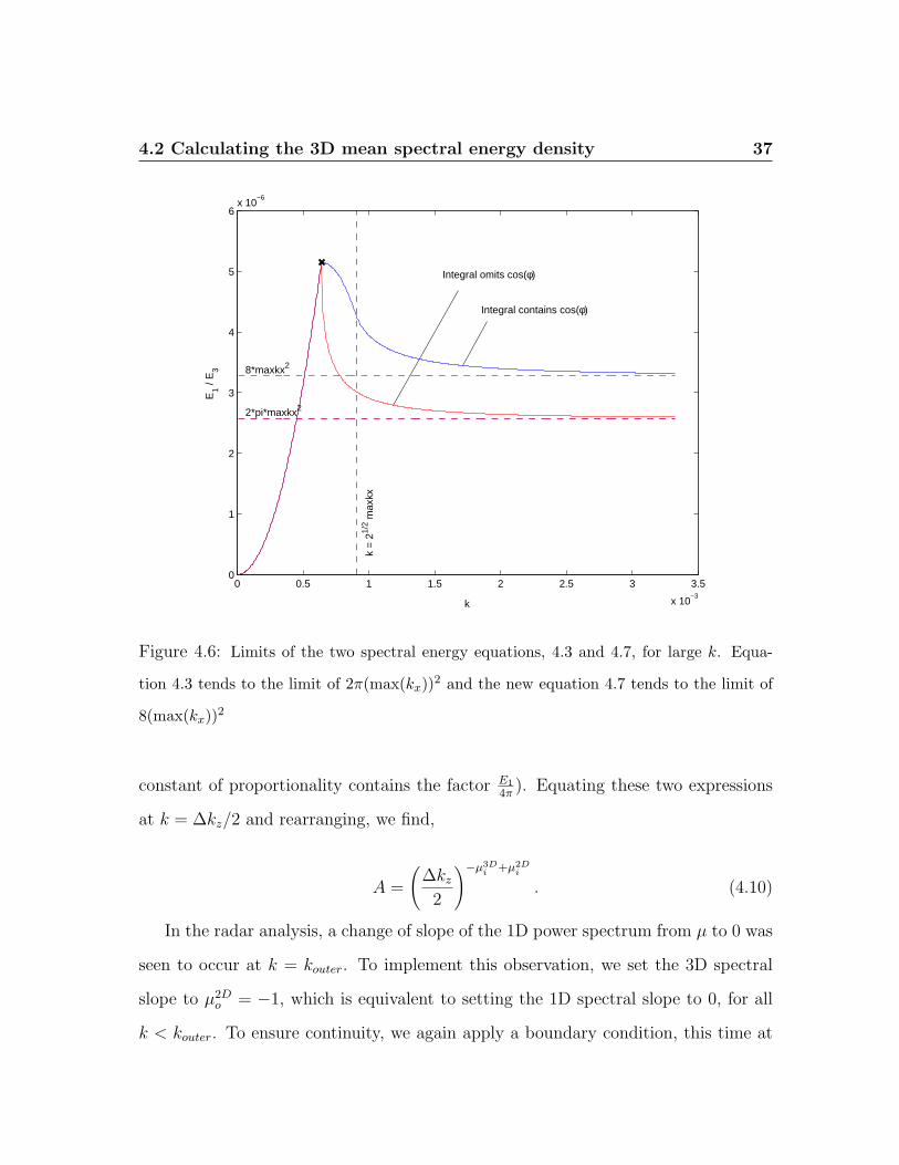
radius max(kx), i.e. 2π max(kx)2. For the full equation for E3, in the limit of large k
we should obtain a surface area of 8 max(kx)2, equivalent to two square cross sections
of side length 2 max kx. The two integrals are compared in figure 4.6. Both equations
tend towards their expected limits for large k. When k = max kx, the bracketed
expression in equation 4.8 is equal to unity and equation 4.3 is recovered.
We now consider the small k, to ensure that we have the right spectral properties
at large scales. When k < ∆kz, a plane, as opposed to a volume, of k-space grid
4.2 Calculating the 3D mean spectral energy density 36
4 5 6 7 8 9 10
x 10−4
0
0.2
0.4
0.6
0.8
1
1.2
1.4
1.6
1.8
2x 10
−5
Wavenumber, k [m−1]
Inte
gran
d
φ = π/4φ = π/8φ = 0
Figure 4.5: The smooth integrand of equation 4.8. The three different lines show the
behaviour of the integrand for three different values of φ as indicated by the key.
points are contained within the k-sphere. The simplest way to deal with this is to
make E3(k) proportional to kµ−1, rather than proportional to kµ−2. It turns out
that this is the appropriate rule for k < ∆kz/2. To ensure that the power spectrum
function is continuous, we need to apply a boundary condition at k = ∆kz/2. Let
us introduce the following notation of µ2Di = µ − 1 and µ3D
i = µ − 2; µ2Do = −1
and µ3Do = −2. The subscript i refers to an inner slope, i.e. the spectral slope for
k > kouter, and the subscript o refers to an outer slope, i.e. the spectral slope for
k < kouter. Now, for k > ∆kz/2, we have E3 ∝ k−µ3Di , and for kouter < k < ∆kz/2 we
have that E3 ∝ Ak−µ2Di , where A is a constant of proportionality (note that the full
4.2 Calculating the 3D mean spectral energy density 37
0 0.5 1 1.5 2 2.5 3 3.5
x 10−3
0
1
2
3
4
5
6x 10
−6
k
E1 /
E3 8*maxkx2
2*pi*maxkx2
k =
21/
2 max
kx
Integral contains cos(φ)
Integral omits cos(φ)
Figure 4.6: Limits of the two spectral energy equations, 4.3 and 4.7, for large k. Equa-
tion 4.3 tends to the limit of 2π(max(kx))2 and the new equation 4.7 tends to the limit of
8(max(kx))2
constant of proportionality contains the factor E1
4π). Equating these two expressions
at k = ∆kz/2 and rearranging, we find,
A =
(∆kz
2
)−µ3Di +µ2D
i
. (4.10)
In the radar analysis, a change of slope of the 1D power spectrum from µ to 0 was
seen to occur at k = kouter. To implement this observation, we set the 3D spectral
slope to µ2Do = −1, which is equivalent to setting the 1D spectral slope to 0, for all
k < kouter. To ensure continuity, we again apply a boundary condition, this time at
4.3 Creating the fractal field 38
kouter. Now, for k > kouter, we have E3 ∝ A (kouter)−µ2D
i , and for k < kouter we have
that E3 ∝ B (kouter)−µ2D
o , where B is a second constant of proportionality. Equating
these at k = kouter we find,
B = A (kouter)−µ2D
i +µ2Do . (4.11)
To summarise, the spectral energy density matrix is described in four parts (see
figure 4.3), according to the magnitude of the wavevector:
E3 =E1
4π×
B k−µ2Do k < kouter
A k−µ2Di kouter < k < ∆kz/2
k−µ3Di ∆kz/2 < k < max(kx)
1Ik−µ3D
i k > max(kx),
where A =
(∆kz
2
)−µ3Di +µ2D
i
, B = A (kouter)−µ2D
i +µ2Do
and I = 1− 4
π
∫ π/4
0
√1− (max(kx)/k cos φ)2dφ.
These equations ensure that the generated fractal has all the required properties.
4.3 Creating the fractal field
Now that we have the mean spectral energy density, we create a matrix of Fourier
coefficients, just as in the 2D model of Hogan and Illingworth (1999). Random phases
of each Fourier component allow multiple realisations of the cloud field. Random
numbers with real and imaginary parts are drawn from a Gaussian distribution with
zero mean and standard deviation of unity. These are then multiplied by the square
root of the mean spectral energy.
4.3 Creating the fractal field 39
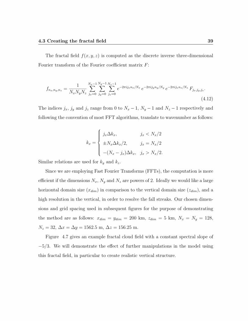
The fractal field f(x, y, z) is computed as the discrete inverse three-dimensional
Fourier transform of the Fourier coefficient matrix F :
fnx,ny,nz =1
NxNyNz
Nx−1∑
jx=0
Ny−1∑
jy=0
Nz−1∑
jz=0
e−2πijxnx/Nx e−2πijyny/Ny e−2πijznz/Nz Fjx,jy ,jz .
(4.12)
The indices jx, jy and jz range from 0 to Nx− 1, Ny − 1 and Nz − 1 respectively and
following the convention of most FFT algorithms, translate to wavenumber as follows:
kx =
jx∆kx, jx < Nx/2
±Nx∆kx/2, jx = Nx/2
−(Nx − jx)∆kx, jx > Nx/2.
Similar relations are used for ky and kz.
Since we are employing Fast Fourier Transforms (FFTs), the computation is more
efficient if the dimensions Nx, Ny and Nz are powers of 2. Ideally we would like a large
horizontal domain size (xdim) in comparison to the vertical domain size (zdim), and a
high resolution in the vertical, in order to resolve the fall streaks. Our chosen dimen-
sions and grid spacing used in subsequent figures for the purpose of demonstrating
the method are as follows: xdim = ydim = 200 km, zdim = 5 km, Nx = Ny = 128,
Nz = 32, ∆x = ∆y = 1562.5 m, ∆z = 156.25 m.
Figure 4.7 gives an example fractal cloud field with a constant spectral slope of
−5/3. We will demonstrate the effect of further manipulations in the model using
this fractal field, in particular to create realistic vertical structure.

4.4 Simulating wind shear 40
0
50
100
150
200
0
50
100
150
2005
10
x [km]y [km]
z [k
m]
Figure 4.7: Initial fractal field with constant spectral slope = −5/3
4.4 Simulating wind shear
Horizontal translation relative to the generating level can be simulated by perturbing
the phases of the Fourier coefficients. Each slice of the cloud field is transformed into
the Fourier domain using the 2D FFT, and treated separately. The coefficients are
multiplied by exp(iθ) where θ = 2π(kxδx+kyδy), and where δx and δy are the required
displacements in the x and y directions (different for each slice). Appropriate δx and
δy are obtained using the fall streak geometry, which in turn requires knowledge of
the wind shear profile. The wind shear profile is provided from UM data (if a specific
cloud is to be simulated), or a hypothetical profile can be used. The vertical cross
section of the cloud field shown in figure 4.8 reveals the fall streak structure obtained
using the UM averaged profiles.
In reality, the height of the generating level is not likely to remain exactly constant
over the horizontal range of the cloud, due to the nature of turbulent motion of the
ambient atmosphere and development of the weather system. A draw-back of this
Fourier technique is that only one generating level can be specified by modelling the
4.5 Perturbation of Fourier amplitudes: Isotropic mixing 41
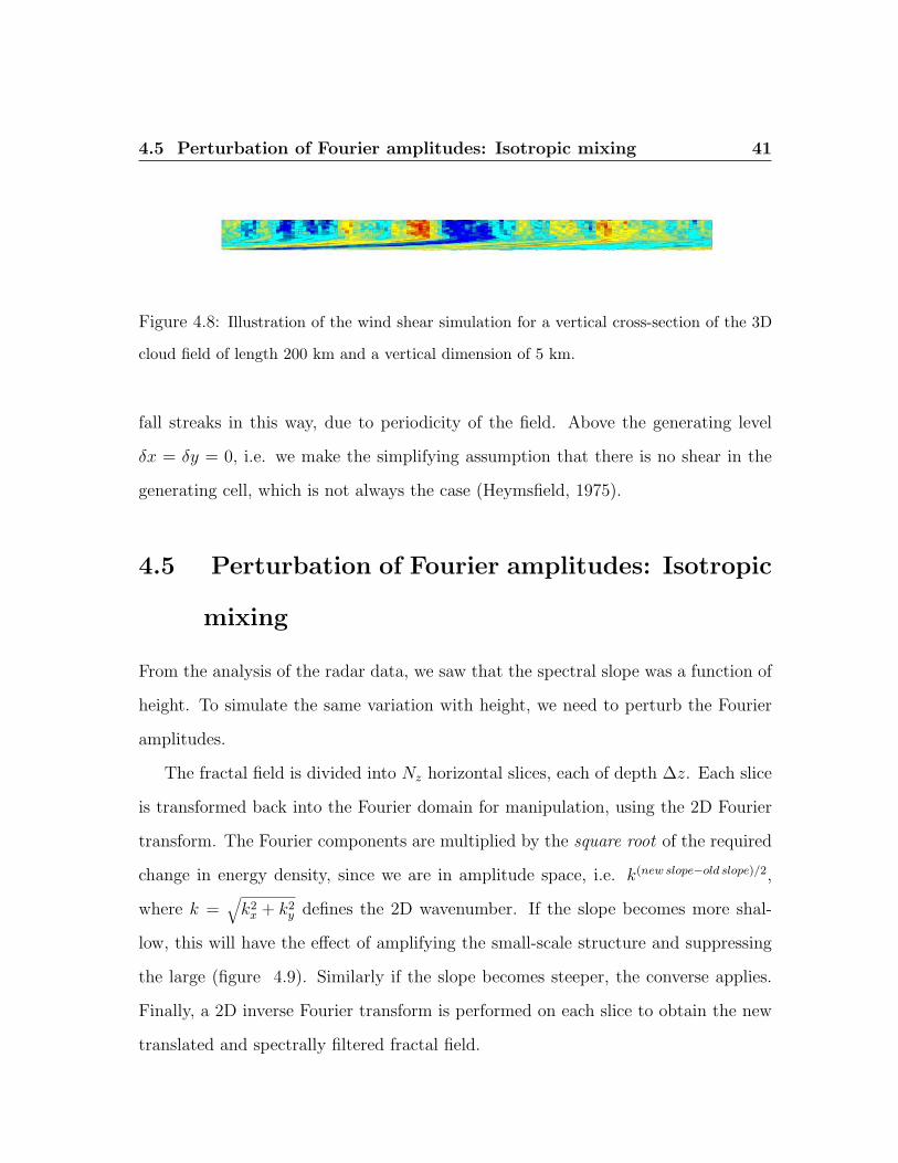
Figure 4.8: Illustration of the wind shear simulation for a vertical cross-section of the 3D
cloud field of length 200 km and a vertical dimension of 5 km.
fall streaks in this way, due to periodicity of the field. Above the generating level
δx = δy = 0, i.e. we make the simplifying assumption that there is no shear in the
generating cell, which is not always the case (Heymsfield, 1975).
4.5 Perturbation of Fourier amplitudes: Isotropic
mixing
From the analysis of the radar data, we saw that the spectral slope was a function of
height. To simulate the same variation with height, we need to perturb the Fourier
amplitudes.
The fractal field is divided into Nz horizontal slices, each of depth ∆z. Each slice
is transformed back into the Fourier domain for manipulation, using the 2D Fourier
transform. The Fourier components are multiplied by the square root of the required
change in energy density, since we are in amplitude space, i.e. k(new slope−old slope)/2,
where k =√
k2x + k2
y defines the 2D wavenumber. If the slope becomes more shal-
low, this will have the effect of amplifying the small-scale structure and suppressing
the large (figure 4.9). Similarly if the slope becomes steeper, the converse applies.
Finally, a 2D inverse Fourier transform is performed on each slice to obtain the new
translated and spectrally filtered fractal field.
4.6 Anisotropic mixing 42
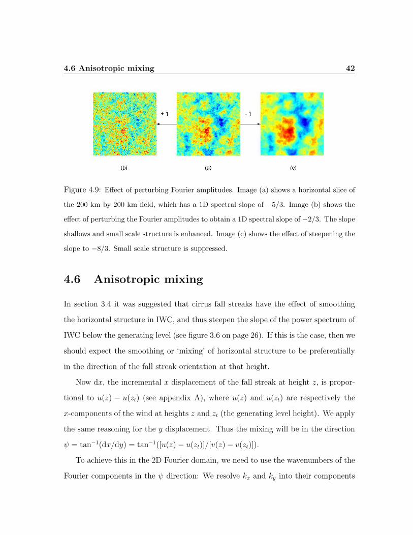
Figure 4.9: Effect of perturbing Fourier amplitudes. Image (a) shows a horizontal slice of
the 200 km by 200 km field, which has a 1D spectral slope of −5/3. Image (b) shows the
effect of perturbing the Fourier amplitudes to obtain a 1D spectral slope of −2/3. The slope
shallows and small scale structure is enhanced. Image (c) shows the effect of steepening the
slope to −8/3. Small scale structure is suppressed.
4.6 Anisotropic mixing
In section 3.4 it was suggested that cirrus fall streaks have the effect of smoothing
the horizontal structure in IWC, and thus steepen the slope of the power spectrum of
IWC below the generating level (see figure 3.6 on page 26). If this is the case, then we
should expect the smoothing or ‘mixing’ of horizontal structure to be preferentially
in the direction of the fall streak orientation at that height.
Now dx, the incremental x displacement of the fall streak at height z, is propor-
tional to u(z) − u(zt) (see appendix A), where u(z) and u(zt) are respectively the
x-components of the wind at heights z and zt (the generating level height). We apply
the same reasoning for the y displacement. Thus the mixing will be in the direction
ψ = tan−1(dx/dy) = tan−1([u(z)− u(zt)]/[v(z)− v(zt)]).
To achieve this in the 2D Fourier domain, we need to use the wavenumbers of the
Fourier components in the ψ direction: We resolve kx and ky into their components
4.6 Anisotropic mixing 43
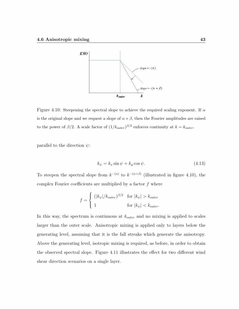
Figure 4.10: Steepening the spectral slope to achieve the required scaling exponent. If α
is the original slope and we request a slope of α+β, then the Fourier amplitudes are raised
to the power of β/2. A scale factor of (1/kouter)β/2 enforces continuity at k = kouter.
parallel to the direction ψ:
kψ = kx sin ψ + ky cos ψ. (4.13)
To steepen the spectral slope from k−(α) to k−(α+β) (illustrated in figure 4.10), the
complex Fourier coefficients are multiplied by a factor f where
f =
(|kψ|/kouter)β/2 for |kψ| > kouter
1 for |kψ| < kouter.
In this way, the spectrum is continuous at kouter and no mixing is applied to scales
larger than the outer scale. Anisotropic mixing is applied only to layers below the
generating level, assuming that it is the fall streaks which generate the anisotropy.
Above the generating level, isotropic mixing is required, as before, in order to obtain
the observed spectral slope. Figure 4.11 illustrates the effect for two different wind
shear direction scenarios on a single layer.
4.7 Scaling the fractal 44
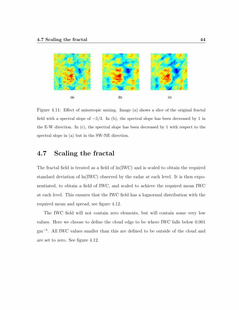
Figure 4.11: Effect of anisotropic mixing. Image (a) shows a slice of the original fractal
field with a spectral slope of −5/3. In (b), the spectral slope has been decreased by 1 in
the E-W direction. In (c), the spectral slope has been decreased by 1 with respect to the
spectral slope in (a) but in the SW-NE direction.
4.7 Scaling the fractal
The fractal field is treated as a field of ln(IWC) and is scaled to obtain the required
standard deviation of ln(IWC) observed by the radar at each level. It is then expo-
nentiated, to obtain a field of IWC, and scaled to achieve the required mean IWC
at each level. This ensures that the IWC field has a lognormal distribution with the
required mean and spread, see figure 4.12.
The IWC field will not contain zero elements, but will contain some very low
values. Here we choose to define the cloud edge to be where IWC falls below 0.001
gm−3. All IWC values smaller than this are defined to be outside of the cloud and
are set to zero. See figure 4.12.
4.8 Testing the model 45
(a)
(b)
(c)
(d)
(e)
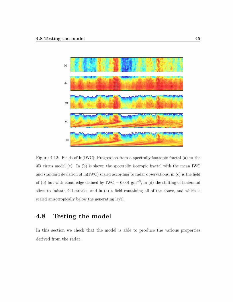
Figure 4.12: Fields of ln(IWC): Progression from a spectrally isotropic fractal (a) to the
3D cirrus model (e). In (b) is shown the spectrally isotropic fractal with the mean IWC
and standard deviation of ln(IWC) scaled according to radar observations, in (c) is the field
of (b) but with cloud edge defined by IWC = 0.001 gm−3, in (d) the shifting of horizontal
slices to imitate fall streaks, and in (e) a field containing all of the above, and which is
scaled anisotropically below the generating level.
4.8 Testing the model
In this section we check that the model is able to produce the various properties
derived from the radar.
4.8 Testing the model 46
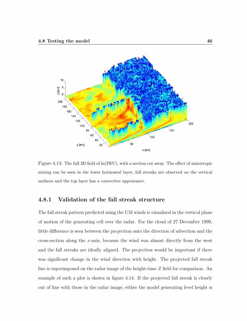
Figure 4.13: The full 3D field of ln(IWC), with a section cut away. The effect of anisotropic
mixing can be seen in the lower horizontal layer, fall streaks are observed on the vertical
surfaces and the top layer has a convective appearance.
4.8.1 Validation of the fall streak structure
The fall streak pattern predicted using the UM winds is visualised in the vertical plane
of motion of the generating cell over the radar. For the cloud of 27 December 1999,
little difference is seen between the projection onto the direction of advection and the
cross-section along the x-axis, because the wind was almost directly from the west
and the fall streaks are ideally aligned. The projection would be important if there
was significant change in the wind direction with height. The projected fall streak
line is superimposed on the radar image of the height-time Z field for comparison. An
example of such a plot is shown in figure 4.14. If the projected fall streak is clearly
out of line with those in the radar image, either the model generating level height is
4.8 Testing the model 47
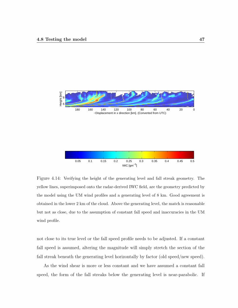
IWC [gm−3]
0.05 0.1 0.15 0.2 0.25 0.3 0.35 0.4 0.45 0.5
020406080100120140160180
6
8
~Displacement in x direction [km]. (Converted from UTC)
Hei
ght [
km]
Figure 4.14: Verifying the height of the generating level and fall streak geometry. The
yellow lines, superimposed onto the radar-derived IWC field, are the geometry predicted by
the model using the UM wind profiles and a generating level of 8 km. Good agreement is
obtained in the lower 2 km of the cloud. Above the generating level, the match is reasonable
but not as close, due to the assumption of constant fall speed and inaccuracies in the UM
wind profile.
not close to its true level or the fall speed profile needs to be adjusted. If a constant
fall speed is assumed, altering the magnitude will simply stretch the section of the
fall streak beneath the generating level horizontally by factor (old speed/new speed).
As the wind shear is more or less constant and we have assumed a constant fall
speed, the form of the fall streaks below the generating level is near-parabolic. If
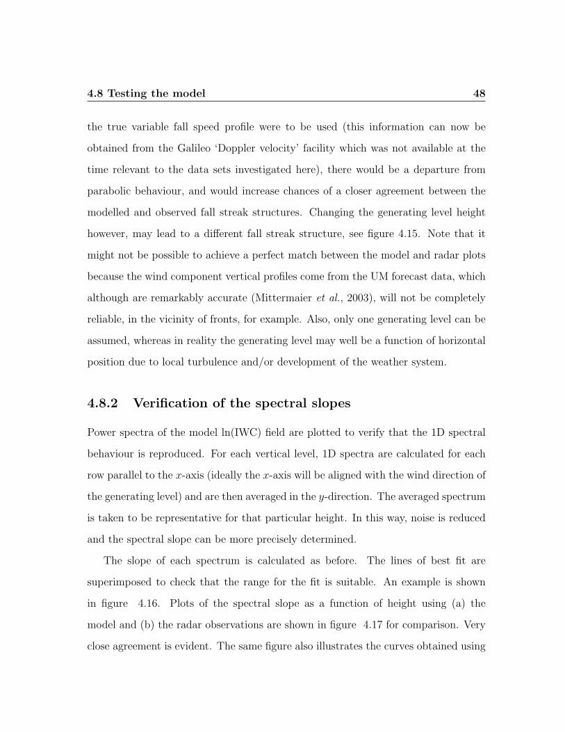
4.8 Testing the model 48
the true variable fall speed profile were to be used (this information can now be
obtained from the Galileo ‘Doppler velocity’ facility which was not available at the
time relevant to the data sets investigated here), there would be a departure from
parabolic behaviour, and would increase chances of a closer agreement between the
modelled and observed fall streak structures. Changing the generating level height
however, may lead to a different fall streak structure, see figure 4.15. Note that it
might not be possible to achieve a perfect match between the model and radar plots
because the wind component vertical profiles come from the UM forecast data, which
although are remarkably accurate (Mittermaier et al., 2003), will not be completely
reliable, in the vicinity of fronts, for example. Also, only one generating level can be
assumed, whereas in reality the generating level may well be a function of horizontal
position due to local turbulence and/or development of the weather system.
4.8.2 Verification of the spectral slopes
Power spectra of the model ln(IWC) field are plotted to verify that the 1D spectral
behaviour is reproduced. For each vertical level, 1D spectra are calculated for each
row parallel to the x-axis (ideally the x-axis will be aligned with the wind direction of
the generating level) and are then averaged in the y-direction. The averaged spectrum
is taken to be representative for that particular height. In this way, noise is reduced
and the spectral slope can be more precisely determined.
The slope of each spectrum is calculated as before. The lines of best fit are
superimposed to check that the range for the fit is suitable. An example is shown
in figure 4.16. Plots of the spectral slope as a function of height using (a) the
model and (b) the radar observations are shown in figure 4.17 for comparison. Very
close agreement is evident. The same figure also illustrates the curves obtained using
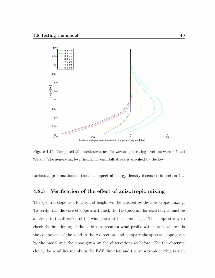
4.8 Testing the model 49
−100 −50 0 505
5.5
6
6.5
7
7.5
8
8.5
9
9.5
10
Horizontal displacement relative to the generating level [km]
Hei
ght [
km]
9.5 km9.0 km8.5 km8.0 km7.5 km7.0 km6.5 km
Figure 4.15: Computed fall streak structure for various generating levels between 6.5 and
9.5 km. The generating level height for each fall streak is specified by the key.
various approximations of the mean spectral energy density discussed in section 4.2.
4.8.3 Verification of the effect of anisotropic mixing
The spectral slope as a function of height will be affected by the anisotropic mixing.
To verify that the correct slope is attained, the 1D spectrum for each height must be
analysed in the direction of the wind shear at the same height. The simplest way to
check the functioning of the code is to create a wind profile with v = 0, where v is
the component of the wind in the y direction, and compare the spectral slope given
by the model and the slope given by the observations as before. For the observed
cloud, the wind lies mainly in the E-W direction and the anisotropic mixing is seen
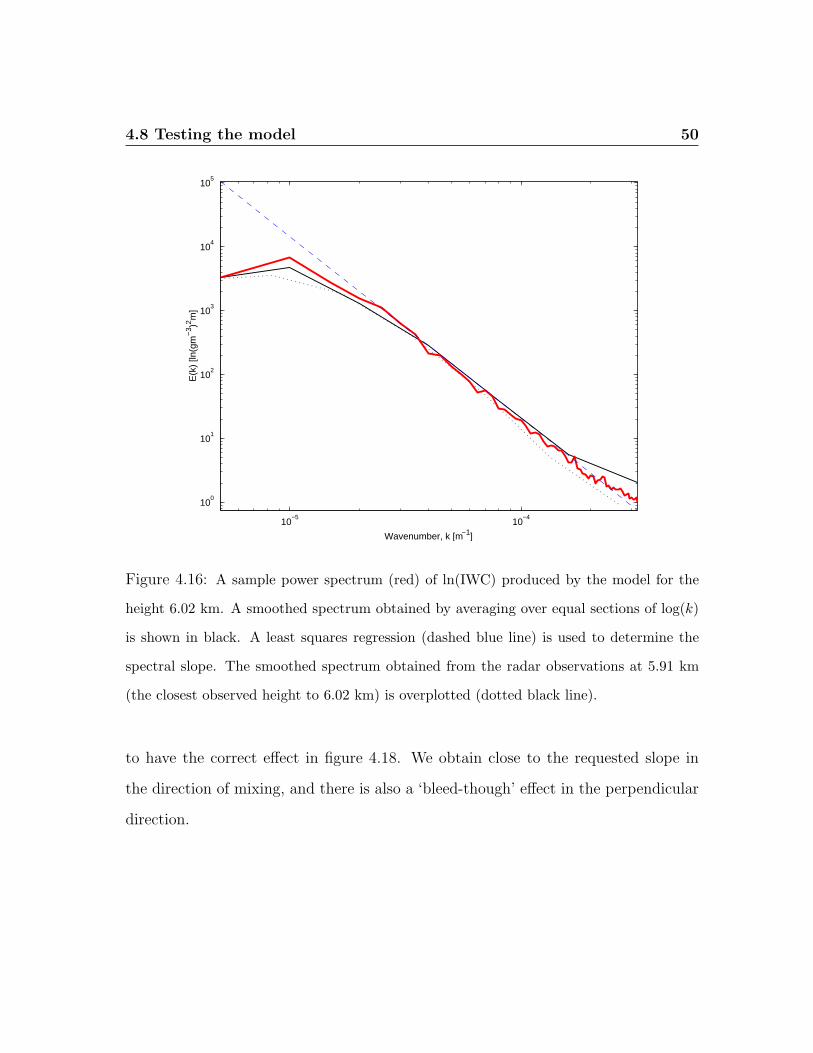
4.8 Testing the model 50
10−5
10−4
100
101
102
103
104
105
Wavenumber, k [m−1]
E(k
) [ln
(gm
−3 )2 m
]
Figure 4.16: A sample power spectrum (red) of ln(IWC) produced by the model for the
height 6.02 km. A smoothed spectrum obtained by averaging over equal sections of log(k)
is shown in black. A least squares regression (dashed blue line) is used to determine the
spectral slope. The smoothed spectrum obtained from the radar observations at 5.91 km
(the closest observed height to 6.02 km) is overplotted (dotted black line).
to have the correct effect in figure 4.18. We obtain close to the requested slope in
the direction of mixing, and there is also a ‘bleed-though’ effect in the perpendicular
direction.
4.9 3D visualisation 51
5 5.5 6 6.5 7 7.5 8 8.5 9 9.5 10−4
−3.5
−3
−2.5
−2
−1.5
−1
height [km]
Spe
ctra
l slo
pe
Figure 4.17: The spectral slope obtained from the radar data analysis (black) is
compared to the spectral slopes produced by the model for the height range of the
cloud. Shown in blue is the slope obtained using the isotropic assumptions. The
improvement obtained by considering the adjustment to E3 when k < ∆kz/2 is
plotted in purple. The green line shows further improvement in using the analytic
solution of equation 4.8 for k > max kx. The red line is the slope obtained by applying
the full numerical solution in place of the analytic solution, and is the slope that we
finally chose.
4.9 3D visualisation
To summarise, a stochastic model has been created that is able to simulate realistic
3D cirrus clouds, for the first time. The flexibility to specify alternative input values
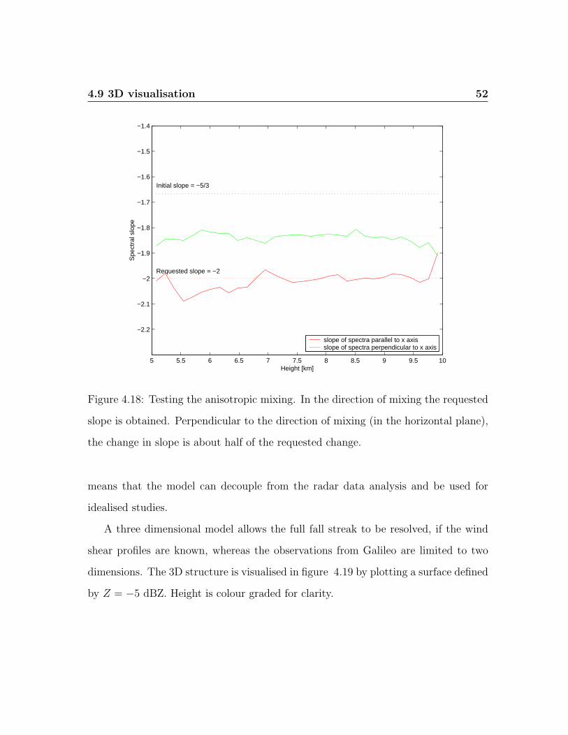
4.9 3D visualisation 52
5 5.5 6 6.5 7 7.5 8 8.5 9 9.5 10
−2.2
−2.1
−2
−1.9
−1.8
−1.7
−1.6
−1.5
−1.4
Height [km]
Spe
ctra
l slo
pe
slope of spectra parallel to x axisslope of spectra perpendicular to x axis
Initial slope = −5/3
Requested slope = −2
Figure 4.18: Testing the anisotropic mixing. In the direction of mixing the requested
slope is obtained. Perpendicular to the direction of mixing (in the horizontal plane),
the change in slope is about half of the requested change.
means that the model can decouple from the radar data analysis and be used for
idealised studies.
A three dimensional model allows the full fall streak to be resolved, if the wind
shear profiles are known, whereas the observations from Galileo are limited to two
dimensions. The 3D structure is visualised in figure 4.19 by plotting a surface defined
by Z = −5 dBZ. Height is colour graded for clarity.
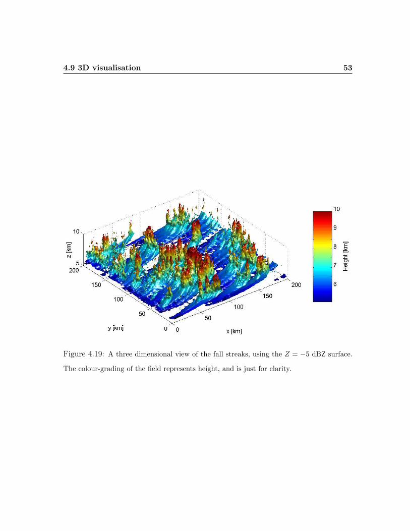
4.9 3D visualisation 53
Figure 4.19: A three dimensional view of the fall streaks, using the Z = −5 dBZ surface.
The colour-grading of the field represents height, and is just for clarity.
Chapter 5
Radiative properties of fractal
cirrus
In this chapter, we consider and investigate how domain-averaged radiative fluxes
are related to particular inputs to the fractal model which exert influence over cloud
inhomogeneity. We introduce the radiation scheme used and then describe the various
cloud fields presented to the scheme.
5.1 The radiative transfer code
As discussed in the introduction, the effects of cloud inhomogeneity may be divided
into two parts:
1. The effect of inhomogeneity due to variations in optical depth.
2. The effect of horizontal photon transport.
Investigations of the second effect, which would require use of a 3D Monte Carlo
radiative transfer scheme, will be the focus of future studies. For now, we turn our
54
5.1 The radiative transfer code 55
attention to the first effect, which may be quantified using the plane-parallel bias.
The plane-parallel bias is the difference between a domain-averaged radiative property
calculated using the independent column approximation (ICA) and that calculated
using the plane-parallel (PP) approximation. We use the Edwards-Slingo radiative
transfer scheme (Edwards and Slingo, 1996) to calculate the radiative fluxes for both
the PP and the ICA assumptions and, in addition, we simulate a GCM calculation.
5.1.1 The Edwards-Slingo radiation scheme
The Edwards-Slingo (ES96) scheme is used operationally in the Met Office Unified
Model to calculate longwave (LW) and shortwave (SW) fluxes and heating rates for
1D atmospheric profiles. In this study, it is used to calculate domain averaged fluxes
assuming the independent column approximation (ICA). The code is run over each
column of the model-produced cloud separately.
The inputs required for the code are
1. height
2. pressure
3. temperature
4. specific humidity
5. IWC
6. effective radius
7. cloud fraction
8. spectral region (LW / SW)
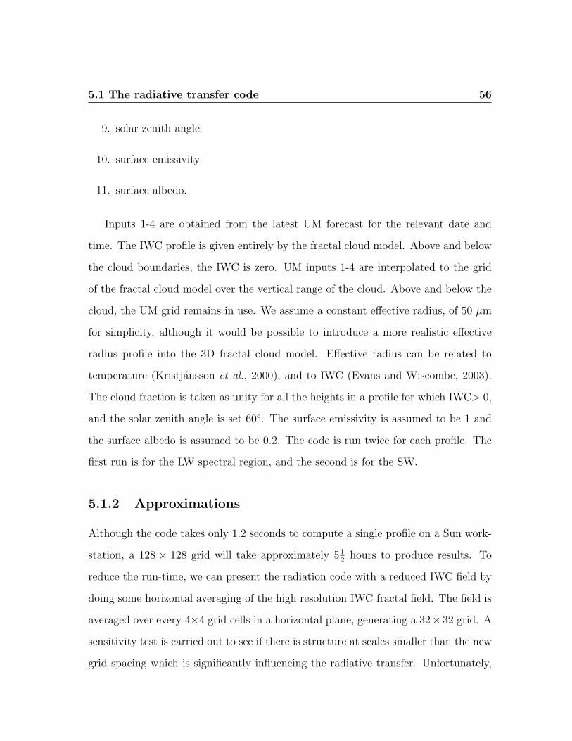
5.1 The radiative transfer code 56
9. solar zenith angle
10. surface emissivity
11. surface albedo.
Inputs 1-4 are obtained from the latest UM forecast for the relevant date and
time. The IWC profile is given entirely by the fractal cloud model. Above and below
the cloud boundaries, the IWC is zero. UM inputs 1-4 are interpolated to the grid
of the fractal cloud model over the vertical range of the cloud. Above and below the
cloud, the UM grid remains in use. We assume a constant effective radius, of 50 µm
for simplicity, although it would be possible to introduce a more realistic effective
radius profile into the 3D fractal cloud model. Effective radius can be related to
temperature (Kristjansson et al., 2000), and to IWC (Evans and Wiscombe, 2003).
The cloud fraction is taken as unity for all the heights in a profile for which IWC> 0,
and the solar zenith angle is set 60◦. The surface emissivity is assumed to be 1 and
the surface albedo is assumed to be 0.2. The code is run twice for each profile. The
first run is for the LW spectral region, and the second is for the SW.
5.1.2 Approximations
Although the code takes only 1.2 seconds to compute a single profile on a Sun work-
station, a 128 × 128 grid will take approximately 512
hours to produce results. To
reduce the run-time, we can present the radiation code with a reduced IWC field by
doing some horizontal averaging of the high resolution IWC fractal field. The field is
averaged over every 4×4 grid cells in a horizontal plane, generating a 32× 32 grid. A
sensitivity test is carried out to see if there is structure at scales smaller than the new
grid spacing which is significantly influencing the radiative transfer. Unfortunately,
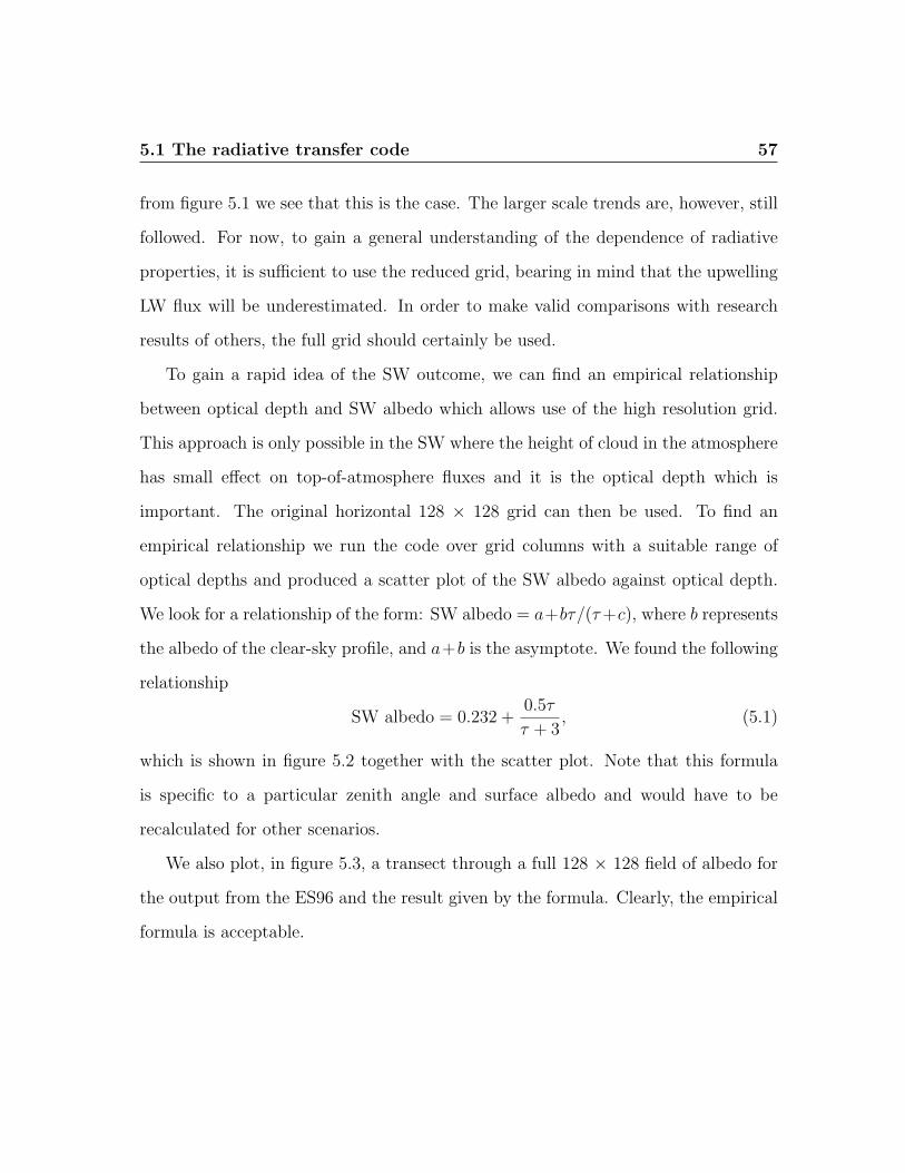
5.1 The radiative transfer code 57
from figure 5.1 we see that this is the case. The larger scale trends are, however, still
followed. For now, to gain a general understanding of the dependence of radiative
properties, it is sufficient to use the reduced grid, bearing in mind that the upwelling
LW flux will be underestimated. In order to make valid comparisons with research
results of others, the full grid should certainly be used.
To gain a rapid idea of the SW outcome, we can find an empirical relationship
between optical depth and SW albedo which allows use of the high resolution grid.
This approach is only possible in the SW where the height of cloud in the atmosphere
has small effect on top-of-atmosphere fluxes and it is the optical depth which is
important. The original horizontal 128 × 128 grid can then be used. To find an
empirical relationship we run the code over grid columns with a suitable range of
optical depths and produced a scatter plot of the SW albedo against optical depth.
We look for a relationship of the form: SW albedo = a+bτ/(τ +c), where b represents
the albedo of the clear-sky profile, and a+b is the asymptote. We found the following
relationship
SW albedo = 0.232 +0.5τ
τ + 3, (5.1)
which is shown in figure 5.2 together with the scatter plot. Note that this formula
is specific to a particular zenith angle and surface albedo and would have to be
recalculated for other scenarios.
We also plot, in figure 5.3, a transect through a full 128 × 128 field of albedo for
the output from the ES96 and the result given by the formula. Clearly, the empirical
formula is acceptable.
5.2 Cloud fields 58
0 20 40 60 80 100 120 140150
160
170
180
190
200
210
220
230
Column number
Upw
ellin
g LW
rad
iatio
n [W
m−
2 ]
Figure 5.1: Sensitivity test to determine whether small scale variations, which are smoothed
out in the reduced resolution grid, have a significant effect on radiation. The upwelling LW
radiation of one row (1×32 cells) of the 32× 32 reduced field is shown in red. This row size
corresponds to a 4×128 strip of cells at the high resolution. The blue dotted line shows
the upwelling LW flux which has been averaged over the width of the strip. A good deal
of smaller scale variability can be seen along the length. When this is averaged over every
4 cells along the length of the strip (green line), we see that the LW flux produced by the
higher resolution grid is consistently larger than that produced by the low resolution grid.
5.2 Cloud fields
Since wind shear is very much responsible for the fall streaks which characterise
cirrus cloud geometry, we chose to investigate the effect of shear on domain-averaged
radiative properties of cirrus. We also investigate the effect of different isotropic
5.2 Cloud fields 59
0 20 40 60 80 100 120 140 1600.2
0.3
0.4
0.5
0.6
0.7
0.8
0.9
optical depth, τ
refle
ctan
ce
Figure 5.2: A scatter plot of reflectance (i.e. SW albedo) against optical depth for a
typical radiation calculation. The SW albedo given by the empirical formula is overplotted:
albedo = 0.232 + 0.5ττ+3 .
spectral slopes. Initially we will carry out all tests using the same set of random
numbers to generate the initial fractal, to be sure that any changes in radiative
properties result from the wind shear or spectral slope and nothing else. The radar
observed cloud of 27 December 1999 is not used for these investigations as it is
physically and optically thick and the LW and SW fluxes reach their saturation
levels. In addition, the generating level for this cloud was found to be 2 km below the
cloud top and most of the solar radiation is attenuated in these top layers before the
effect of shear, which occurs predominantly in the lower 2 km of the cloud, has chance
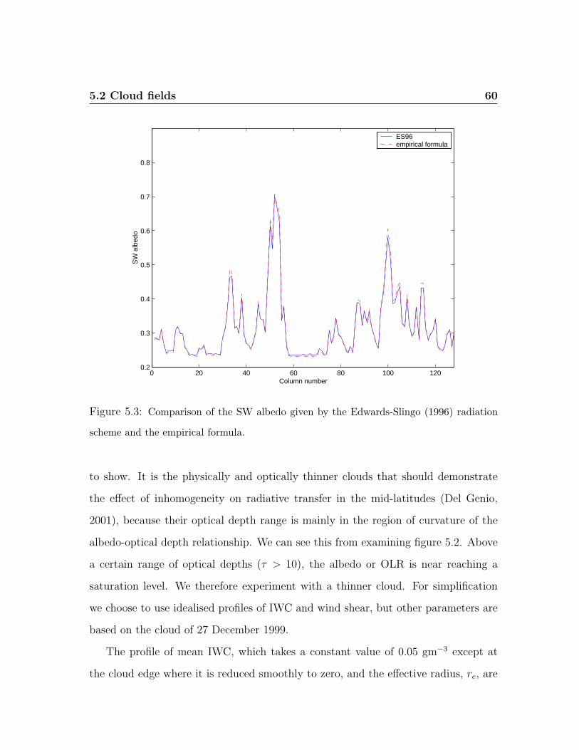
5.2 Cloud fields 60
0 20 40 60 80 100 1200.2
0.3
0.4
0.5
0.6
0.7
0.8
Column number
SW
alb
edo
ES96empirical formula
Figure 5.3: Comparison of the SW albedo given by the Edwards-Slingo (1996) radiation
scheme and the empirical formula.
to show. It is the physically and optically thinner clouds that should demonstrate
the effect of inhomogeneity on radiative transfer in the mid-latitudes (Del Genio,
2001), because their optical depth range is mainly in the region of curvature of the
albedo-optical depth relationship. We can see this from examining figure 5.2. Above
a certain range of optical depths (τ > 10), the albedo or OLR is near reaching a
saturation level. We therefore experiment with a thinner cloud. For simplification
we choose to use idealised profiles of IWC and wind shear, but other parameters are
based on the cloud of 27 December 1999.
The profile of mean IWC, which takes a constant value of 0.05 gm−3 except at
the cloud edge where it is reduced smoothly to zero, and the effective radius, re, are
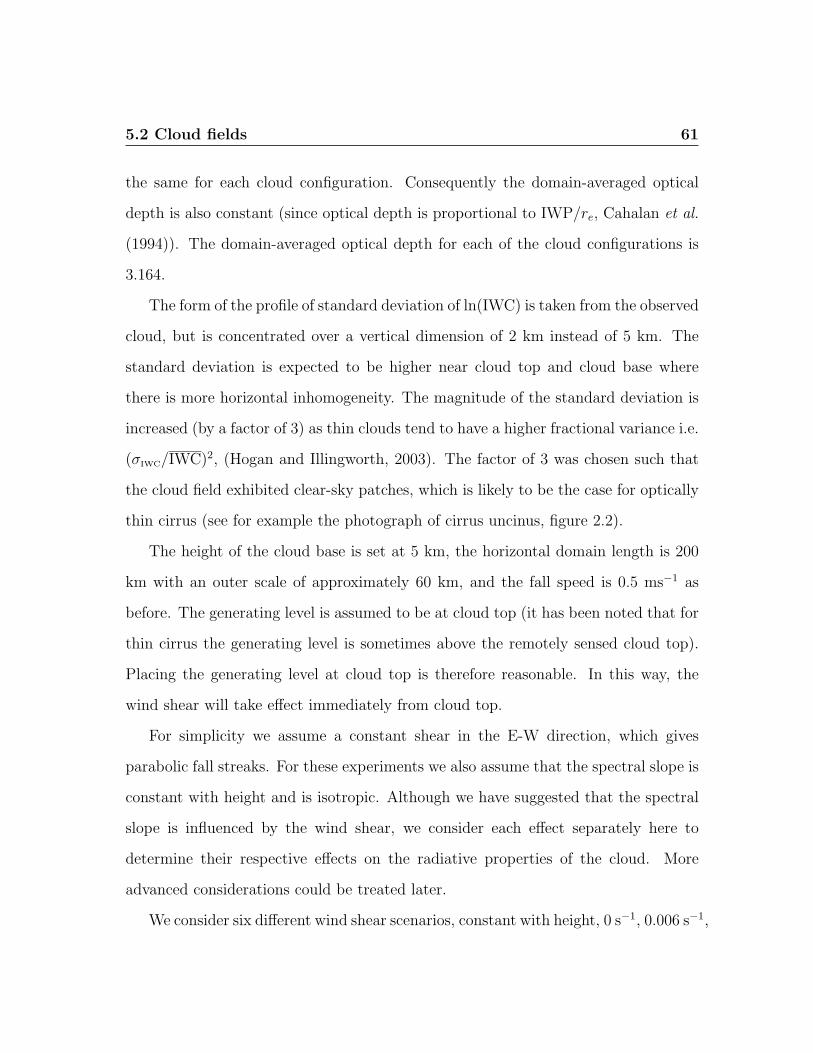
5.2 Cloud fields 61
the same for each cloud configuration. Consequently the domain-averaged optical
depth is also constant (since optical depth is proportional to IWP/re, Cahalan et al.
(1994)). The domain-averaged optical depth for each of the cloud configurations is
3.164.
The form of the profile of standard deviation of ln(IWC) is taken from the observed
cloud, but is concentrated over a vertical dimension of 2 km instead of 5 km. The
standard deviation is expected to be higher near cloud top and cloud base where
there is more horizontal inhomogeneity. The magnitude of the standard deviation is
increased (by a factor of 3) as thin clouds tend to have a higher fractional variance i.e.
(σIWC/IWC)2, (Hogan and Illingworth, 2003). The factor of 3 was chosen such that
the cloud field exhibited clear-sky patches, which is likely to be the case for optically
thin cirrus (see for example the photograph of cirrus uncinus, figure 2.2).
The height of the cloud base is set at 5 km, the horizontal domain length is 200
km with an outer scale of approximately 60 km, and the fall speed is 0.5 ms−1 as
before. The generating level is assumed to be at cloud top (it has been noted that for
thin cirrus the generating level is sometimes above the remotely sensed cloud top).
Placing the generating level at cloud top is therefore reasonable. In this way, the
wind shear will take effect immediately from cloud top.
For simplicity we assume a constant shear in the E-W direction, which gives
parabolic fall streaks. For these experiments we also assume that the spectral slope is
constant with height and is isotropic. Although we have suggested that the spectral
slope is influenced by the wind shear, we consider each effect separately here to
determine their respective effects on the radiative properties of the cloud. More
advanced considerations could be treated later.
We consider six different wind shear scenarios, constant with height, 0 s−1, 0.006 s−1,
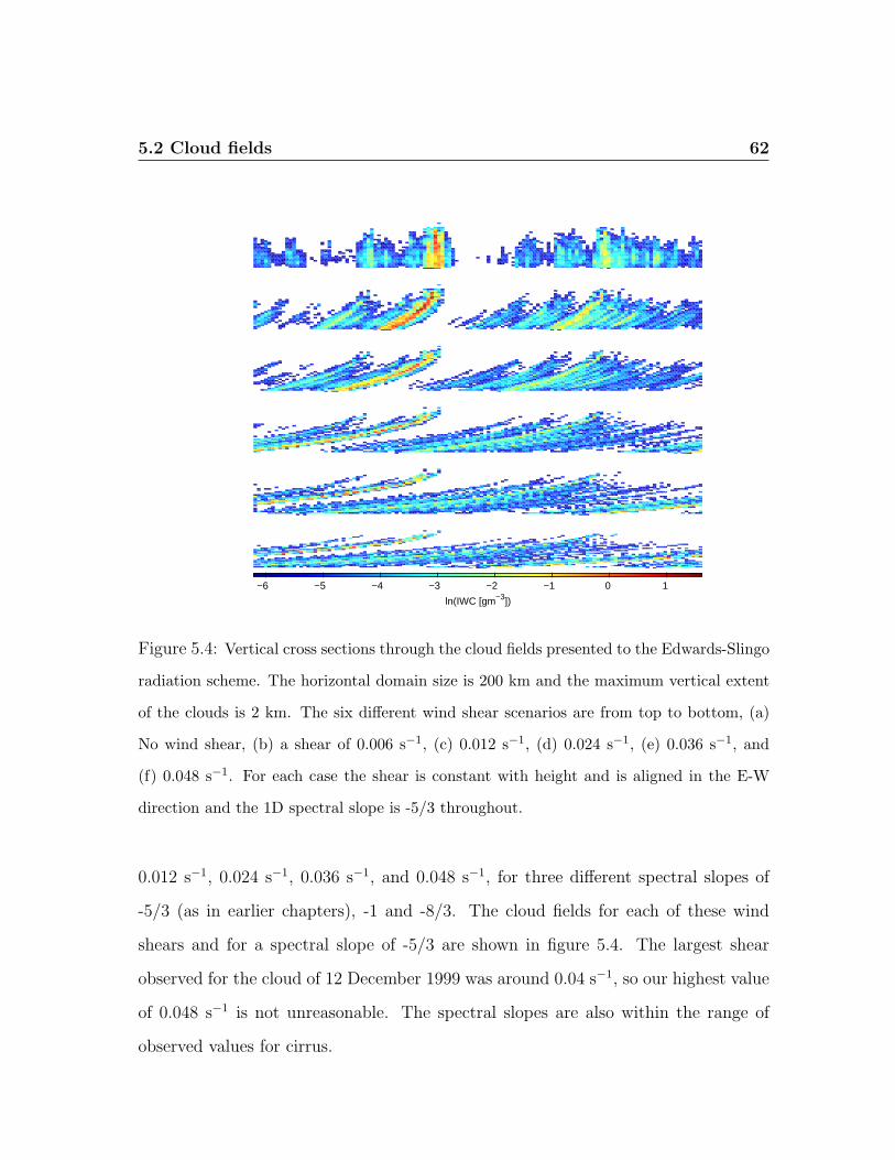
5.2 Cloud fields 62
ln(IWC [gm−3])
−6 −5 −4 −3 −2 −1 0 1
Figure 5.4: Vertical cross sections through the cloud fields presented to the Edwards-Slingo
radiation scheme. The horizontal domain size is 200 km and the maximum vertical extent
of the clouds is 2 km. The six different wind shear scenarios are from top to bottom, (a)
No wind shear, (b) a shear of 0.006 s−1, (c) 0.012 s−1, (d) 0.024 s−1, (e) 0.036 s−1, and
(f) 0.048 s−1. For each case the shear is constant with height and is aligned in the E-W
direction and the 1D spectral slope is -5/3 throughout.
0.012 s−1, 0.024 s−1, 0.036 s−1, and 0.048 s−1, for three different spectral slopes of
-5/3 (as in earlier chapters), -1 and -8/3. The cloud fields for each of these wind
shears and for a spectral slope of -5/3 are shown in figure 5.4. The largest shear
observed for the cloud of 12 December 1999 was around 0.04 s−1, so our highest value
of 0.048 s−1 is not unreasonable. The spectral slopes are also within the range of
observed values for cirrus.

5.2 Cloud fields 63
5.2.1 GCM resolution simulation
To demonstrate the inadequacy of the representation of cirrus cloud inhomogeneity
in a GCM, we simulate a GCM representation of the cloud fields created by the 3D
model, and compare the results of the experiments. A GCM grid box will contain a
cloud fraction and, in the cloudy part of the box, each horizontal layer of the cloud is
assumed to be uniform. An overlap assumption is required to determine how a layer
is placed with respect to its neighbours. The simplest approach, the one employed
by most GCMs, is to assume ‘maximum random’ overlap (Hogan and Illingworth,
2000). Maximum overlap is assumed between adjacent GCM cloud layers if the cloud
is vertically continuous, and random overlap is applied to clouds at different heights
if they are separated by a completely cloud-free layer. In this study, the cirrus cloud
fields created are vertically continuous and so random overlap would not have been
employed by a GCM. Maximum overlap alone is therefore assumed. In each layer,
the cloudy grid cells are shifted to the same side of the GCM grid box (figure 5.5).
Most GCMs use atmospheric pressure as their vertical coordinate, so their vertical
resolution will vary, but typically vertical resolutions will be between 500 and 750m
at cirrus altitudes (Hogan and Illingworth, 2000). In our GCM representation, the
vertical resolution of the 3D fractal cloud model will need to be reduced. Vertical
averaging over a suitable integer number of layers is then performed to reduce the
vertical resolution to a typical value. As we have 32 vertical layers, the simplest
method is to average over every 8 layers which, with a vertical dimension of 2 km,
will give a 500 m resolution and 4 levels. Results from the simulation will then be
indicative of the upper range of a GCMs performance. The IWC threshold distin-
guishing between cloudy and non-cloudy grid cells is still enforced by the 3D fractal
model at the higher vertical resolution, and not by the GCM simulation.
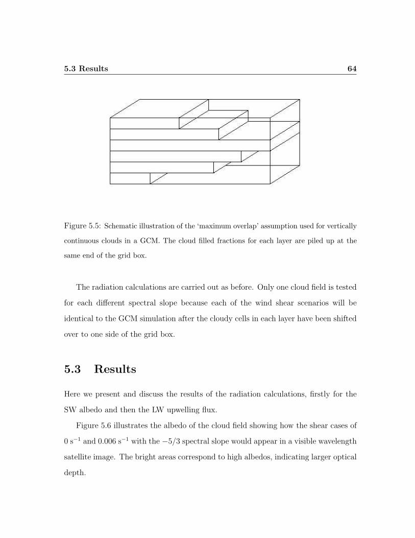
5.3 Results 64
Figure 5.5: Schematic illustration of the ‘maximum overlap’ assumption used for vertically
continuous clouds in a GCM. The cloud filled fractions for each layer are piled up at the
same end of the grid box.
The radiation calculations are carried out as before. Only one cloud field is tested
for each different spectral slope because each of the wind shear scenarios will be
identical to the GCM simulation after the cloudy cells in each layer have been shifted
over to one side of the grid box.
5.3 Results
Here we present and discuss the results of the radiation calculations, firstly for the
SW albedo and then the LW upwelling flux.
Figure 5.6 illustrates the albedo of the cloud field showing how the shear cases of
0 s−1 and 0.006 s−1 with the −5/3 spectral slope would appear in a visible wavelength
satellite image. The bright areas correspond to high albedos, indicating larger optical
depth.
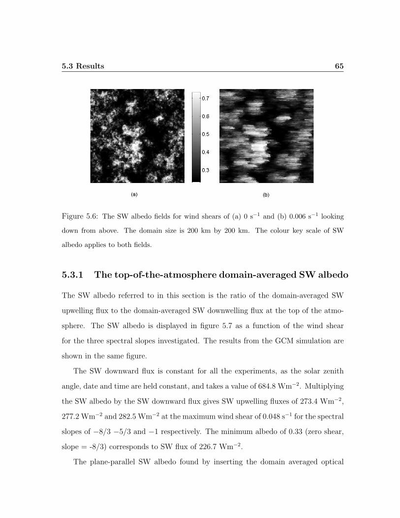
5.3 Results 65
Figure 5.6: The SW albedo fields for wind shears of (a) 0 s−1 and (b) 0.006 s−1 looking
down from above. The domain size is 200 km by 200 km. The colour key scale of SW
albedo applies to both fields.
5.3.1 The top-of-the-atmosphere domain-averaged SW albedo
The SW albedo referred to in this section is the ratio of the domain-averaged SW
upwelling flux to the domain-averaged SW downwelling flux at the top of the atmo-
sphere. The SW albedo is displayed in figure 5.7 as a function of the wind shear
for the three spectral slopes investigated. The results from the GCM simulation are
shown in the same figure.
The SW downward flux is constant for all the experiments, as the solar zenith
angle, date and time are held constant, and takes a value of 684.8 Wm−2. Multiplying
the SW albedo by the SW downward flux gives SW upwelling fluxes of 273.4 Wm−2,
277.2 Wm−2 and 282.5 Wm−2 at the maximum wind shear of 0.048 s−1 for the spectral
slopes of −8/3 −5/3 and −1 respectively. The minimum albedo of 0.33 (zero shear,
slope = -8/3) corresponds to SW flux of 226.7 Wm−2.
The plane-parallel SW albedo found by inserting the domain averaged optical
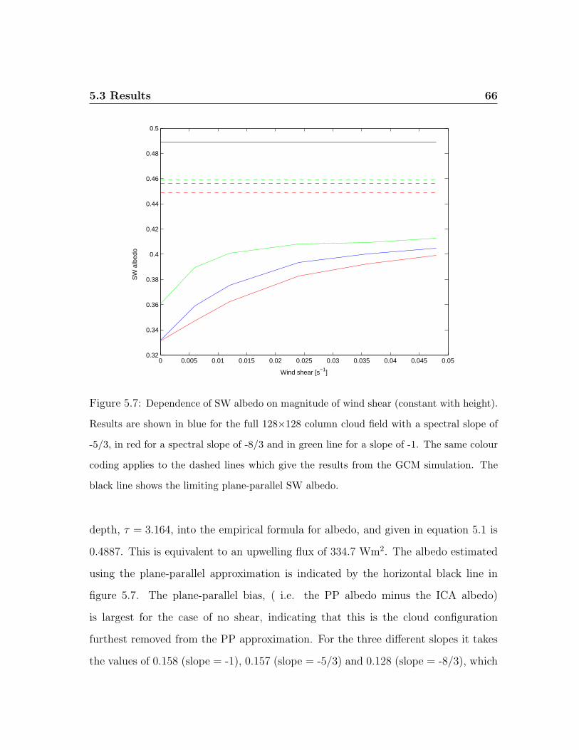
5.3 Results 66
0 0.005 0.01 0.015 0.02 0.025 0.03 0.035 0.04 0.045 0.050.32
0.34
0.36
0.38
0.4
0.42
0.44
0.46
0.48
0.5
Wind shear [s−1]
SW
alb
edo
Figure 5.7: Dependence of SW albedo on magnitude of wind shear (constant with height).
Results are shown in blue for the full 128×128 column cloud field with a spectral slope of
-5/3, in red for a spectral slope of -8/3 and in green line for a slope of -1. The same colour
coding applies to the dashed lines which give the results from the GCM simulation. The
black line shows the limiting plane-parallel SW albedo.
depth, τ = 3.164, into the empirical formula for albedo, and given in equation 5.1 is
0.4887. This is equivalent to an upwelling flux of 334.7 Wm2. The albedo estimated
using the plane-parallel approximation is indicated by the horizontal black line in
figure 5.7. The plane-parallel bias, ( i.e. the PP albedo minus the ICA albedo)
is largest for the case of no shear, indicating that this is the cloud configuration
furthest removed from the PP approximation. For the three different slopes it takes
the values of 0.158 (slope = -1), 0.157 (slope = -5/3) and 0.128 (slope = -8/3), which

5.3 Results 67
are very similar to the biases of 10-15% found by Cahalan (1994) and Barker and
Davies (1992). This can be expected as there is little or no shear in stratocumulus
and the cloud altitude has little effect on the SW fluxes. The PP bias is about 8%
(slope = -5/3) for the largest shear. Carlin et al. (2002) reported a range of cirrus
solar albedo biases of up to 25% which were dependent on solar zenith angle (SZA)
and underlying surface albedo. For an SZA of zero (which should be similar to our
ICA approximation) they calculated albedo biases of a few percent, which compares
favourably with our results.
We can see that GCMs capture some of the vertical inhomogeneity and can im-
prove their estimate of domain averaged-albedo with respect to the PP albedo as a
consequence of including a cloud fraction for each of their vertical levels.
The SW albedo increases as the cloud configuration becomes more sheared and
consequently more similar to the PP form. This is a consequence of the non-linearity
of the albedo-optical depth relationship, (see figure 1.1). For each wind shear exper-
iment we see that as the spectral slope steepens, the SW albedo is reduced. Barker
and Davies (1992) observed the same trends when they carried out a similar experi-
ment for stratocumulus clouds. Their data were obtained using 2D isotropic, scaling,
broken cloud fields. They investigated the relationship between spectral slope and
reflectance (SW albedo) testing slopes between 0 and 4, for a solar zenith angle of
about 78◦. They held constant the cloud fraction (equivalent in this study to con-
stant wind shear) and the domain-averaged optical depth. Their cloud fields, however
were input to a Monte Carlo photon transport code, rather than a 1D ICA radiative
transfer scheme. They showed that as the spectral slope steepens, the SW albedo
tends to a ‘plane-parallel’ limit which they defined as Rpp × Ac, where Rpp is the
plane-parallel reflectance (SW albedo) and Ac is the cloud fraction.
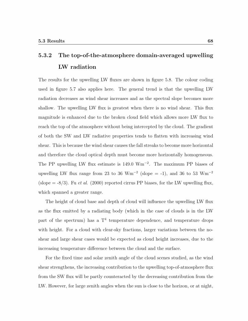
5.3 Results 68
5.3.2 The top-of-the-atmosphere domain-averaged upwelling
LW radiation
The results for the upwelling LW fluxes are shown in figure 5.8. The colour coding
used in figure 5.7 also applies here. The general trend is that the upwelling LW
radiation decreases as wind shear increases and as the spectral slope becomes more
shallow. The upwelling LW flux is greatest when there is no wind shear. This flux
magnitude is enhanced due to the broken cloud field which allows more LW flux to
reach the top of the atmosphere without being intercepted by the cloud. The gradient
of both the SW and LW radiative properties tends to flatten with increasing wind
shear. This is because the wind shear causes the fall streaks to become more horizontal
and therefore the cloud optical depth must become more horizontally homogeneous.
The PP upwelling LW flux estimate is 149.0 Wm−2. The maximum PP biases of
upwelling LW flux range from 23 to 36 Wm−2 (slope = -1), and 36 to 53 Wm−2
(slope = -8/3). Fu et al. (2000) reported cirrus PP biases, for the LW upwelling flux,
which spanned a greater range.
The height of cloud base and depth of cloud will influence the upwelling LW flux
as the flux emitted by a radiating body (which in the case of clouds is in the LW
part of the spectrum) has a T4 temperature dependence, and temperature drops
with height. For a cloud with clear-sky fractions, larger variations between the no-
shear and large shear cases would be expected as cloud height increases, due to the
increasing temperature difference between the cloud and the surface.
For the fixed time and solar zenith angle of the cloud scenes studied, as the wind
shear strengthens, the increasing contribution to the upwelling top-of-atmosphere flux
from the SW flux will be partly counteracted by the decreasing contribution from the
LW. However, for large zenith angles when the sun is close to the horizon, or at night,
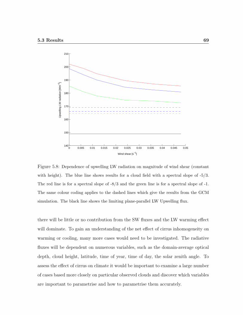
5.3 Results 69
0 0.005 0.01 0.015 0.02 0.025 0.03 0.035 0.04 0.045 0.05140
150
160
170
180
190
200
210
Upw
ellin
g LW
rad
iatio
n [W
m−
2 ]
Wind shear [s−1]
Figure 5.8: Dependence of upwelling LW radiation on magnitude of wind shear (constant
with height). The blue line shows results for a cloud field with a spectral slope of -5/3.
The red line is for a spectral slope of -8/3 and the green line is for a spectral slope of -1.
The same colour coding applies to the dashed lines which give the results from the GCM
simulation. The black line shows the limiting plane-parallel LW Upwelling flux.
there will be little or no contribution from the SW fluxes and the LW warming effect
will dominate. To gain an understanding of the net effect of cirrus inhomogeneity on
warming or cooling, many more cases would need to be investigated. The radiative
fluxes will be dependent on numerous variables, such as the domain-average optical
depth, cloud height, latitude, time of year, time of day, the solar zenith angle. To
assess the effect of cirrus on climate it would be important to examine a large number
of cases based more closely on particular observed clouds and discover which variables
are important to parametrise and how to parametrise them accurately.
Chapter 6
Conclusion
The accurate representation of clouds in GCMs is crucial to the understanding of
future climate change. Presently, GCMs cannot satisfactorily represent cloud inho-
mogeneity, which has resulted in gross approximations for cloud radiative properties.
This has motivated research into development of cloud resolving models which can
be used to find new and improve existing parametrisations of cloud inhomogeneity.
Early research mainly focused on stratocumulus, the most common type of cloud. It
is only relatively recently that researchers have turned their attention to cirrus, yet
only 2D models have been reported.
6.1 The 3D fractal cirrus model
Here, and for the first time, a 3D fractal model for cirrus clouds has been developed,
which incorporates parameters defining the vertical structure of the cloud. Unique
to the model are the implementations of 3D fall streak structure, variable grid res-
olution in both the horizontal and vertical planes, a characteristic power-law break
of scale indicative of the maximum scale length of variability, and anisotropic spec-
70
6.1 The 3D fractal cirrus model 71
tral mixing in the horizontal plane. Height dependent statistics such as the mean
IWC, and the standard deviation of ln(IWC) are based on vertically pointing 94 GHz
radar observations of one particular mid-latitude cirrus cloud, chosen because the
fall streaks were ideally aligned with the direction of motion of the cloud across the
radar. The Unified Model vertical profiles of wind and temperature were also impor-
tant input parameters in determining the IWC from radar reflectivities and the fall
streak structure.
Observations of the dependence on the 1D spectral slope on height were partic-
ularly intriguing. At cloud top, the spectral slope is constant with height (about
-4/3), until the generating level is reached. The slope below this height gradually
steepened, reaching values of around -3. Various spectral slopes over a similar range
have previously been reported but without mention of the dependence of the scaling
exponent on height, or any other parameter. In this study we assume that the change
can be attributed to mixing due to fall streaks intersecting and/or varying ice crystal
fall speeds.
Limitations of the model have already been discussed at various points of this
report. They include reliability on the accuracy of UM wind profiles. This would
be required if the model were to be used in the interpretation of 2D satellite images
to estimate the third dimension of the cloud field. It would not be so important
in the application of the model to radiative transfer investigations where it is often
more instructive to use a generalised or idealised shear. Three main assumptions
were outlined in the introduction, that of a constant effective radius (50 µm), a
lognormal PDF for the IWC and a constant generating level. The Galileo radar
has now been Dopplerised, allowing fall speeds and sizes of precipitation particles
to be determined. The next stage of development could include the implementation
6.2 Investigations of cirrus cloud radiative properties 72
of a height dependent fall speed profile and a height dependent PDF for ice crystal
effective radius. There has already been some research into the later, for example,
Evans (2001) produces a stochastic field for the particle effective radius by using a
height (which is related to temperature) and LWC dependent lookup table operating
on a Gaussian field. This ensures that appropriate values of re are produced for each
LWC value, so that for example, re = 0 does not occur inside of clouds.
Many further radar observations should be examined in order to verify trends
which have been observed for the 27 December 1999. For example, in Hogan and
Illingworth (1999) we noted an outer scale of 25 km for cirrus, but our cirrus cloud
data from 27 December 1999, indicated an outer scale of about 60 km. If anisotropic
mixing truly occurs in the direction of the fall streak orientation then, the measure-
ment of outer scale will be dependent on the alignment of the fall streaks with the
generating level direction of motion. The work of Di Guiseppe and Tompkins (2003)
indicated that the dominant scale of structure, albeit for stratocumulus, has an influ-
ence over the radiative properties of the cloud. This emphasises the need to determine
a realistic range of such parameters for cirrus.
6.2 Investigations of cirrus cloud radiative prop-
erties
We employed the Edwards-Slingo 1D radiative transfer scheme to assess the effect
of cirrus inhomogeneity due to optical depth variations (as opposed to the effect of
horizontal photon transport) on SW and LW radiative fluxes, and compared results
with those obtained from a GCM simulation and a plane-parallel configuration. We
presented to the radiative transfer code six different constant wind shear scenarios
6.2 Investigations of cirrus cloud radiative properties 73
ranging from 0 s−1 to 0.048 s−1. It was found that increasing shear reduces horizontal
inhomogeneity and thus also the plane-parallel biases. As the spectral slope steepens,
the shortwave albedo decreases and the upwelling longwave flux increases, tending
away from the plane-parallel values.
Examples of further tests which could be done are investigations on the effect
of varying the standard deviation, varying the spectral slope with height at a rate
related to the wind shear, exploring the effect of different IWC profiles, changing of
wind shear direction with height. It would be interesting to note how net radiative
forcing is dependent on optical depth with other parameters held constant as the LW
upwelling radiation saturates at smaller optical depths than the SW albedo.
Acknowledgements
To my supervisor Robin Hogan, thank you for a very enjoyable four months. Your
encouragement and guidance have been much appreciated. To my parents, thank you
so much for your support - particularly the telephone calls at just the right moment.
I would also like to thank Malcolm Brooks for his help with the Edwards-Slingo
radiation code. I gratefully acknowledge support from NERC under award number
NER/S/M/2002/10650.
Appendix A
Ice Fall Streak Geometry
Consider the top of a cirrus fall streak as a ‘generating cell’ which moves with the
wind at that height and releases crystals. The 3D shape of the fallstreak is found by
considering the trajectory of a single crystal as it falls, in the frame of reference of
the generating cell.
Marshall (1953) derives the trajectory of the ice crystals as follows: If x repre-
sents distance in a particular horizontal direction, z is the depth (vertical distance
increasing downwards), u(z) = dxdt
is the component of the wind in the x direction
and the fall speed w(z) = dzdt
then the equation of the ice particle trajectory can be
described as
x− x0 =∫ z
0
u(z)
w(z)dz, (A.1)
where x0 is the x coordinate of the generating element. Marshall (1953) examines
the case when wind shear and fall speed are both constant. With u = Sz and w = b,
where S and b are both constants (and S is the shear), equation A.1 simplifies to
74
75
x− x0 =S
2bz2, (A.2)
which describes a parabola.
The pattern formed by ice particles precipitating from the generating cell is the
trajectory of the particles, in the frame of reference of the generating cell. In any
other frame of reference, the pattern and trajectory become two different things.
We would like to find the fall streak geometry for any wind shear scenario. To
work in the reference frame of the generating cell we replace u(z) in equation A.1 by
u(z)−u(zt) where zt is the generating level height and u(zt) is the velocity component
in the x direction at that height. Let x0 = 0 and allow x to represent the horizontal
displacement between a crystal and the generating cell, such that
x(z) =∫ z′=zt
z′=zdx =
∫ z′=zt
z′=z
u(z′)− u(zt)
w(z′)dz′. (A.3)
Similarly, if y represents horizontal displacement relative to the generating cell
and perpendicular to x, and v(z) = dydt
, then
y(z) =∫ z′=zt
z′=zdy =
∫ z′=zt
z′=z
v(z′)− v(zt)
w(z′)dz′. (A.4)
If we know the profiles of ui, vi and wi, at heights zi from levels i = 0 to i = t
at the generating level, which must also be known, then equations A.3 and A.4 can
be solved iteratively using finite differences. We set xt=0 and yt = 0 and work
downwards from the generating level using the following iterations,
xi = xi+1 +(
ui+1 + ui
2− ut
)(zi+1 − zi)
2
wi+1 + wi
(A.5)
yi = yi+1 +(
vi+1 + vi
2− vt
)(zi+1 − zi)
2
wi+1 + wi
. (A.6)
76
If the fall speed wi is unknown, a constant value could be assumed. Typical fall
speed is about 1 ms−1 (e.g. Mittermaier et al. (2003), Marshall (1953), Heymsfield
(1975)).
The fall streak geometry can then be approximated in the model by shifting each
horizontal slice with respect to the slice at generating level height by (δx, δy), where
for slice i,
δxi = xi − x0 = xi, and
δyi = yi − y0 = yi.
Appendix B
Treatment of incomplete data sets
This appendix describes how to find the mean and standard deviation for broken
data sets assumed to have a Normal PDF. It is credited entirely to Robin Hogan but
is included here for the sake of completeness.
Suppose we have a series of data values x, which in the context of this study
could represent radar reflectivity in dBZ, or ln(IWC) for which we would like to
estimate the mean and standard deviation. Due to the sensitivity of the radar, there
are missing values in the series where all we know is that x < xc, where xc is the
minimum detectable signal. We suppose that the underlying probability density
function (PDF) is a Normal, with mean xm and standard deviation σx. We know
the fraction f of the data series for which a valid value has been recorded (i.e. the
fraction of the underlying PDF for which x > xc) and the mean of these measured
values x′m.
If we know xc, x′m, and f we can derive xm and σx. The probability density
function, P (x), is a Normal distribution:
77
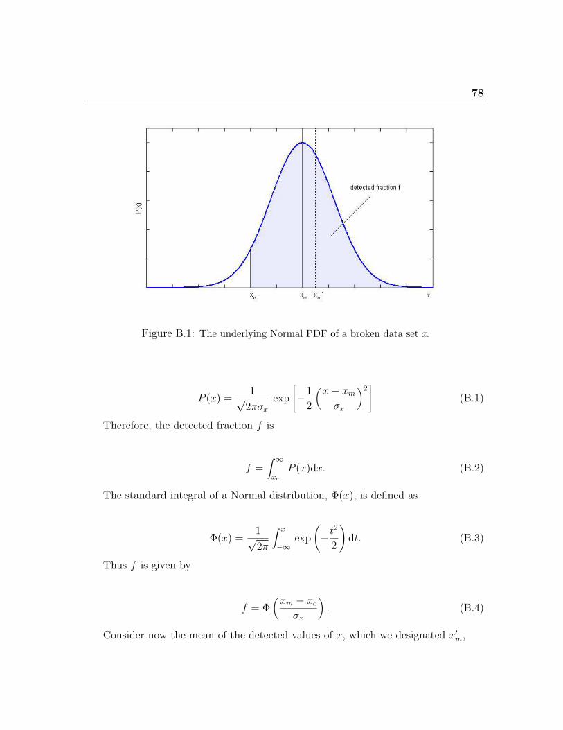
78
Figure B.1: The underlying Normal PDF of a broken data set x.
P (x) =1√
2πσx
exp
[−1
2
(x− xm
σx
)2]
(B.1)
Therefore, the detected fraction f is
f =∫ ∞
xc
P (x)dx. (B.2)
The standard integral of a Normal distribution, Φ(x), is defined as
Φ(x) =1√2π
∫ x
−∞exp
(−t2
2
)dt. (B.3)
Thus f is given by
f = Φ(
xm − xc
σx
). (B.4)
Consider now the mean of the detected values of x, which we designated x′m,
79
x′m =
∫∞xc
xP (x)dx∫∞xc
P (x)dx
=1
f
1√2πσx
∫ ∞
xc
x exp
(−1
2
[x− xm
σx
]2)
dx. (B.5)
Now, let t =(
x−xm
σx
)2. Then dt = 2
σx
(x−xm
σxdx
)and xdx = σ 2
x
2dt + xmdx. Substi-
tuting for xdx in equation B.5 and adjusting the integrations limits results in
x′m = xm +1
f
1√2πσx
∫ ∞
(xc−xmσx
)2exp
(−1
2t)
dt
= xm +σx
f√
2πexp
(−1
2
(xc − xm
σx
)2)
. (B.6)
Thus we have two equations (B.4) and (B.6) and two unknowns. Firstly we use
the inverse function of (B.3), Φ−1(x) to transform (B.4) :
xm − xc
σx
= Φ−1(f) = A (B.7)
Substitute this into (B.6):
x′m − xm
σx
=1
f√
2πexp
(−1
2
[Φ−1(f)
]2)
= B (B.8)
Rearranging (B.7) and (B.8) we find
xm = xc +x′m − xc
1 + B/A; σx =
x′m− xc
A + B(B.9)
When f > 0.5, this may not be the best way to estimate xm and σx because
as f becomes close to unity it becomes more an indicator of the lower tail of the
distribution, rather than a good indicator of the width of the distribution σx, which
is what is required. An alternative approach when f > 0.5 is to assume that the

80
median of the underlying distribution is equal to the mean xm. Since we have more
than half the values, the median is easy to determine, and thus the mean can be
estimated. The width of the underlying distribution σx may be estimated by first
calculating the mean of the data greater than xm, which we denote x′m(f = 12):
x′m(f =1
2) =
∫∞xm
xP (x)dx∫∞xm
P (x)dx(B.10)
From (B.6) it is easy to show that
x′m(f =1
2) = xm + σx
√2
π. (B.11)
Thus σx is estimated from xm and x′m(f = 12). When f > 0.9 or f > 0.95 there is
probably enough data to take the mean x′m and standard deviation σ′x of the detected
values and assume x′m = xm and σ′x = σx.
References
Barker, H. W. and Davies, J. A., 1992: Solar radiative fluxes for stochastic, scale-
invariant broken cloud fields. J. Atmos. Sci., 49, 1115-1125.
Cahalan, R. F. and Joseph, J. H., 1989: Fractal statistics of cloud fields. Mon. Wea.
Rev., 117, 261-272.
Cahalan, R. F. and Snider, J. B., 1989: Marine stratocumulus structure. Remote
Sens. Environ., 28, 95-107.
Cahalan, R. F., Ridgeway, R., Wiscombe, W. J. and Bell, T. L., 1994: The albedo
of fractal stratocumulus clouds. J. Atmos. Sci., 51, 2434-2455.
Cahalan, R. F., 1994: Bounded cascade clouds: albedo and effective thickness.
Nonlin. Proc. Geophys., 1, 156-167.
Carlin, B., Fu, Q., Lohmann, U., Mace, G. G., Sassen, K. and Comstock, J. M.,
2002: High-cloud horizontal inhomogeneity and solar albedo bias. J. Climate.,
15, 2321-2339.
Cess, R. D., et al., 1996: Cloud feedback in atmospheric general circulation models:
An update J. Geophys. Res., 101, 12791-12794.
81
82
Danne, O., Mace, G. G., Clothiaux, E. E., Dong, X., Ackerman, T. P. and Quante,
M., 1996: Observing structures and vertical motions within stratiform clouds
using a vertical pointing 94-GHz cloud radar. Beitr. Phys. Atmos., 69, 229-
237.
Davis, A., Marshak, A., Cahalan, R. F. and Wiscombe, W., 1997: The Landsat
scale break in stratocumulus as a three-dimensional radiative transfer effect:
Implications for cloud remote sensing. J. Atmos. Sci., 54, 241-260.
Del Genio, A. D., 2001: GCM simulations of cirrus for climate studies. Cirrus, D.
Lynch et al., Eds., Oxford University Press, 310-326.
Di Guiseppe, F. and Tompkins, A. M., 2003: Effect of spatial organisation on so-
lar radiative transfer in three dimensional idealized stratocumulus cloud fields.
Submitted to J. Atmos. Sci..
Edwards, J. M. and Slingo, A., 1996: Studies with a flexible new radiation code. I:
Choosing a configuration for a large-scale model. Quart. J. Roy. Meteor. Soc.,
122, 689-719.
Evans, K. F., Mc Farlane, S. A. and Wiscombe, W., 2001: The importance of three-
dimensional solar radiative transfer in small cumulus cloud fields derived from
the Nauru MMCR and MWR. Proc. of the 11th Atmospheric Radiation Mea-
surement (ARM) Science Team Meeting., March 19-23, 2001, Atlanta Georgia.
Evans, K. F. and Wiscombe W. J., 2003: An algorithm for generating stochastic
cloud fields. Atmos. Res. special issue on Clouds and Radiation (submitted) .
Fu, Q. Carlin, B. and Mace, C., 2000: Cirrus horizontal inhomogeneity and OLR
bias. Geophys. Res. Lett., 27, 3341-3344.
83
Heymsfield, A. J., 1975: Cirrus uncinus generating cells and the evolution of cir-
riform clouds. Part II: The structure and circulation of the cirrus uncinus
generating head. J. Atmos. Sci., 4, 809-819.
Heymsfield, A. J. and Mcfarquhar, G. M., 2001: Mid-latitude and tropical cirrus:
Microphysical properties. Cirrus, D. Lynch et al., Eds., Oxford University
Press, 78-101.
Hogan, R. J. and Illingworth, A. J., 1999: The potential of spaceborne dual-
wavelength radar to make global measurements of cirrus clouds. J. Atmos.
Oceanic. Technol., 16, 518-531.
Hogan, R. J. and Illingworth, A. J., 2000: Deriving cloud overlap statistics from
radar. Quart. J. Roy. Meteor. Soc., 126, 2903-2909.
Hogan, R. J. and Illingworth, A. J., 2003: Parametrising ice cloud inhomogeneity
and the overlap of inhomogeneities using cloud radar data. J. Atmos. Sci., 60,
756-767.
Kristjansson, J. E., Edwards, J. M., and Mitchell, D. L., 2000: Impact of a new
scheme for optical properties of ice crystals on climates of two GCMs. J. Geo-
phys. Res., 105, 10063-10079.
Larson et al., 2001: Systematic biases in the microphysics and thermodynamics
of numerical models that ignore subgrid-scale variability. J. Atmos. Sci., 58,
1117-1128.
Liu, C-L, and Illingworth, A. J., 2000: Toward more accurate retrievals of ice water
content from radar measurements of clouds. J. Appl. Meteorol., 39, 1130-1146.
84
Lovejoy, S., 1982: The area-perimeter relationship for rain and cloud areas. Science,
216, 185-187.
Lynch, D. K., 2001: Cirrus: History and Definition. Cirrus, D. Lynch et al., Eds.,
Oxford University Press, 3-10.
Marshall, J. S., 1953: Precipitation trajectories and patterns. J. Meteor., 10, 25-30.
Mittermaier, M. P., Hogan R. J. and Illingworth, A. J., 2003: Exploring new syner-
gies between radar data and mesoscale model forecasts. Proc. 31st AMS conf.
on Radar Meteorol. Seattle, 6-12 August 2003
Pincus, R., Barker, H. W. and Morcette, J., 2002: A fast, flexible, approximate
technique for computing radiative transfer in inhomogeneous cloud fields. Sub-
mitted to J. Geophys. Res.
Pomroy, H. R. and Illingworth, A. J., 2000: Quantifying bias in emissivity from
radar observations. Geophys. Res. Lett., 27, 2101-2104.
Press, W. H., 1992: Numerical recipes in Fortran: The art of scientific computing.
Second edition. Cambridge University Press.
Salby, M. L., 1996: Fundamentals of Atmospheric Physics. Academic Press, 36-46.
Sassen, K., 2001: Cirrus clouds: A modern perspective. Cirrus, D. Lynch et al.,
Eds., Oxford University Press, 11-40.
Sassen, K. and Mace, G. G., 2001: Ground-based remote sensing of cirrus clouds.
Cirrus, D. Lynch et al., Eds., Oxford University Press, 168-196.
85
Starr, D. O’C. and Quante, M., 2001: Dynamical processes in cirrus clouds: Con-
cepts and models. Cirrus, D. Lynch et al., Eds., Oxford University Press,
375-396.
Stephens, G. L., 1988: Radiative transfer through arbitrarily shaped optical media.
Part II: Group theory and simple closures. J. Atmos. Sci., 45, 1837-1848.
Stephens, G. L. et al., 2002: The CloudSat mission and the A-train. Bull. Amer.
Meteorol. Soc., 83, 1771-1790.
Tessier, Y., Lovejoy, S. and Schertzer, D., 1993: Universal Multifractals: Theory
and observations for rain and clouds. J. Appl. Meteorol., 32, 223-250.
Tiedtke, M., 1996: An extension of cloud-radiation parametrization in the ECMWF
model: The representation of subgrid-scale variation of optical depth. Mon.
Wea. Rev., 124, 745-750.
World Meteorological Organisation (WMO), 1992: International Meteorological Vo-
cabulary. Second Edition., WMO no. 128, Geneva.