Development and Validation of the Wind Energy Calculator (WEC

Development and Validation of the Wind Energy Calculator

(WEC) for use as a module in the larger Complimentary Energy

Decision Support Tool (CEDST) project

by

Stephanie Diane Shaw

A Thesis

presented to

The University of Guelph

In partial fulfilment of requirements

for the degree of

Master of Applied Science

in

Engineering

Guelph, Ontario, Canada

© Stephanie Diane Shaw, August, 2012

ABSTRACT

Development and Validation of the Wind Energy Calculator (WEC) for use as a

module in the larger Complimentary Energy Decision Support Tool (CEDST)

project

Stephanie Diane Shaw Advisor:

University of Guelph, 2012 Dr. Bill Van Heyst

The Complimentary Energy Decision Support Tool (CEDST) was conceived to be

a renewable energy calculator designed specifically for rural sites and agricultural

operations in Ontario, though could easily assess urban sites as well, and equipped with

the ability to compare the feasibility of different technologies. The Wind Energy

Calculator (WEC) component of the CEDST project was the focus of this thesis and was

developed since research revealed no current wind prediction tools that met CEDST

needs. Verification of WEC predictions found prediction accuracy to have bounds of +/-

60% on actual turbine energy production and was equivalent to the actual generation for

21% of cases. The discrepancy could have resulted from unusual annual wind speeds,

which had no significant impact on project economics when analysed. Many cases

revealed that 10 kW turbines are not feasible projects under the Feed-in Tariff program

and that turbines begin to become economical around 35 kW.

iii

Acknowledgements

There were many people and organizations that helped make this project possible.

The University of Guelph, Natural Sciences and Engineering Research Council of

Canada (NSERC), the Poultry Industry Council (PIC), Ontario Ministry of Agriculture,

Food and Rural Affairs (OMAFRA), and Egg Farmers of Ontario all provided funding to

support work on this project.

Thanks goes out to Mr. Steve Free, Mr. Enzo Baldassini, and the City of Guelph with

their help gathering data and information on the Guelph Emergency Services Facility

wind turbine. The Nova Scotia wind turbine data was also graciously provided by Mr.

Glenn Jennings, of Bayview Poultry Farms, through Mr. Kenneth Corscadden, at the

Nova Scotia Agricultural College. Additionally, Dr. Mel Tyree was instrumental in

gathering and sharing the New York State wind turbine data with this project, without

which this project would not have become what it is, thank you Dr. Tyree!

Thank you to my supervisors Dr. Bill Van Heyst and Dr. David Lubitz for all their support

and guidance. Additionally, thanks goes out to the other students who contributed to the

project in different ways: David Wood, Robert Morgan, and Andrew Sims.

A big thank you is reserved for Daniel Roth, who was a wonderful person to work with

and a person to count on when getting work done, needing to brainstorm or meeting

deadlines. Without Dan this project would not have been possible, so Thank You!

iv

Table of Contents List of Tables ................................................................................................................. vii

List of Figures ................................................................................................................. ix

List of Symbols ............................................................................................................. xiii

Chapter 1 – Introduction ................................................................................................. 1

1.1 Project Intentions .................................................................................................. 1

1.2 Introduction to Energy ........................................................................................... 2

1.3 Background ........................................................................................................... 5

1.3.1 Green Energy ................................................................................................. 6

1.3.2 Green Energy Act and Feed-in-Tariff (FIT) Program ....................................... 6

1.3.3 MicroFIT Program ........................................................................................... 7

1.3.4 Purpose of CEDST ........................................................................................10

1.3.5 Wind Energy Calculator (WEC) .....................................................................13

Chapter 2 – Literature Review .......................................................................................14

2.1 Purpose, Guidelines and Criteria..........................................................................14

2.2 Literature – Existing Renewable Energy Calculators ............................................19

2.2.1 RETScreen ....................................................................................................19

2.2.2 HOMER .........................................................................................................23

2.2.3 CanWEA: Ballpark Cost Calculator ................................................................24

2.2.4 Solar Estimator.org: My Solar & Wind Estimator ............................................25

2.2.5 Windustry: Wind Project Calculator (WPC) ....................................................26

2.2.6 DWIA: Wind Power and Economics Calculators ............................................27

2.3 Literature Review Conclusions .............................................................................29

2.4 Literature Review Implications .............................................................................30

Chapter 3 – Decision Making Process ...........................................................................33

3.1 Existing Models ....................................................................................................33

3.2 Wind Energy Calculator (WEC) Decision Making Model ......................................37

Chapter 4 – Wind Speed Prediction and Data Sources .................................................42

4.1 Wind Speed Prediction .........................................................................................42

4.2 Wind Speed Data .................................................................................................44

4.3 Ontario Wind Speed Data Sources ......................................................................45

4.3.1 Canadian Wind Energy Atlas .........................................................................45

v

4.3.2 Ontario Renewable Energy Atlas ...................................................................47

4.3.3 NASA ............................................................................................................48

4.3.4 Environment Canada .....................................................................................48

4.4 Summary of Wind Speed Data Sources ...............................................................49

Chapter 5 – WEC Database and Interpolation ...............................................................50

5.1 Database .............................................................................................................50

5.2 Interpolation .........................................................................................................50

5.3 Wind Speed Calculations .....................................................................................53

5.4 Summary .............................................................................................................54

Chapter 6 – Wind Turbine Properties ............................................................................55

6.1 Turbine Size .........................................................................................................55

6.2 Wind Turbine Models ...........................................................................................56

6.3 Rotor Diameter and Hub Height ...........................................................................56

6.4 Power Curve ........................................................................................................59

Chapter 7 – Wind Power Calculations ...........................................................................61

7.1 Calculating Wind Power .......................................................................................61

Chapter 8 – Wind Turbine Economics ...........................................................................64

8.1 Cost of a Wind Turbine ........................................................................................64

8.2 Economics Calculations .......................................................................................64

Chapter 9 – Wind Turbine Siting ....................................................................................69

9.1 Importance of Turbine Siting ................................................................................69

9.2 Ontario Turbine Classifications and Guidelines ....................................................69

9.3 Small Wind Turbine Guidelines ............................................................................71

9.3.1 Property Lines ...............................................................................................71

9.3.2 Buildings, Man-made Structures, and Vegetation – Setbacks ........................71

9.3.3 Buildings, Man-made Structures, and Vegetation – Height

Recommendations .................................................................................................72

9.3.4 Roof Top Turbines .........................................................................................73

9.4 Relating Setback and Height to the WEC .............................................................73

9.5 What Makes an Ideal Wind Site? .........................................................................73

9.6 Concerns Over Turbine Location..........................................................................75

Chapter 10 – Wind Turbine: Case Study Availability ......................................................76

10.1 Case Study Search ............................................................................................76

vi

10.1.1 Ontario.........................................................................................................76

10.1.2 Nova Scotia .................................................................................................77

10.1.3 New York .....................................................................................................78

Chapter 11 – Wind Turbine: Case Study Analysis .........................................................81

11.1 Case Study Intentions ........................................................................................81

11.2 Inverse Distance Weighted (IDW) Power Factor ................................................81

11.3 Guelph ...............................................................................................................87

11.4 Nova Scotia........................................................................................................90

11.5 New York State ..................................................................................................91

11.6 RETScreen versus WEC ....................................................................................96

11.7 Relative Prediction Accuracy ..............................................................................97

11.8 Case Study Conclusions .................................................................................. 101

Chapter 12 – Examination of WEC Economic Results ................................................. 103

12.1 Introduction and Normal WEC Economic Predictions ....................................... 103

12.2 Impacts of Abnormal Wind Production ............................................................. 105

12.3 Influence of Turbine Size on the Feasibility Assessment of a Site .................... 106

12.4 Interpretation of Results ................................................................................... 109

12.5 Summary ......................................................................................................... 110

Chapter 13 – Sources of Error ..................................................................................... 111

13.1 Sources of Error in WEC .................................................................................. 111

13.1.1 Wind Speed Calculations ........................................................................... 111

13.1.2 Power Calculations .................................................................................... 112

13.1.3 Economics ................................................................................................. 113

13.2 Error Summary ................................................................................................. 113

Chapter 14 – Conclusion ............................................................................................. 114

Chapter 15 – Future Work ........................................................................................... 117

References .................................................................................................................. 118

Appendix A – Appendix of Figures ............................................................................... 128

Appendix B – Appendix of Tables ................................................................................ 136

vii

List of Tables

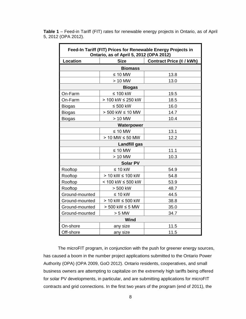
Table 1 – Feed-in Tariff (FIT) rates for renewable energy projects in Ontario, as of April

5, 2012 (OPA 2012). ....................................................................................................... 8

Table 2 – Literature review table summarizing the results of how each calculator

investigated matched the criteria for an acceptable CEDST wind prediction tool. ..........22

Table 3 – MCDM model criteria for the analytic hierarchy process for assessment of

wind turbine project feasibility as determined by Lee et al. (2009). [WEG = wind energy

generator] ......................................................................................................................35

Table 4 – Assessment of wind speed data sources covering Ontario. ...........................45

Table 5 – Wind turbine size and application comparison (adapted from CanWEA 2010c,

2010d). ..........................................................................................................................56

Table 6 – Rotor diameter and potential tower heights for the small wind turbine models

that will be incorporated into the WEC database. ..........................................................57

Table 7 – Costs associated with owning and operating a small wind turbine system

(CanWEA 2010d). .........................................................................................................64

Table 8 – Compounding period and corresponding m value. .........................................66

Table 9 – Canadian federal and Ontario provincial personal income tax rates (CRA

2011). ............................................................................................................................67

Table 10 – Definition of wind turbine classes within the Ontario government regulations

(GoO 2011b). ................................................................................................................70

Table 11 – Setback regulations for Class 3, 4 and 5 wind turbines in Ontario (GoO

2011a). ..........................................................................................................................70

Table 12 – Percent difference between the predictions using p=1 for the IDW

Interpolation method and p=1.5 and p=2 respectively. In most cases, aside from Nova

Scotia, most predictions were within +/- 5 % of each other. ...........................................86

viii

Table 13 – Relationship between actual energy production of a turbine and what the

turbine is anticipated to produce through ratio and percent deviation and also to site

geography. ....................................................................................................................95

Table 14 – Comparison of wind speeds used in the CEDST WEC to those from

Environment Canada monitoring sites ......................................................................... 100

Table 15 – Economic assessment results for the sites of turbines 16 and 17 in New York

State both for average WEC predictions and those testing the impact of abnormal

production on project feasibility.................................................................................... 104

Table 16 – Results of the economic assessments for sites 16 and 17 investigating how

project feasibility changes with turbine size. ................................................................ 107

Table 17 – Results of the economic assessments for site 1 investigating at what size a

small wind turbine project becomes feasible. ............................................................... 108

Table 18 – Table with data comparing: the impact of p in the IDW method on WEC

predictions, the ratio of actual production to WEC (p=1.5) predicted value, and the

percent deviation between the WEC (p=1.5) prediction and actual turbine production. 136

ix

List of Figures

Figure 1 – Renewable Energy Sources – Decision Support System (RES-DSS) model by

Voivontas et al. (1998) illustrating the decision making process for assessing the wind

energy potential of a site. Picture adopted from Voivontas et al. (1998).........................36

Figure 2 – Decision making model for the WEC. ...........................................................41

Figure 3 – Illustration of the positioning of the database points, with respect to the site of

interest xu, that are used in the IDW interpolation method. ............................................52

Figure 4 – Method of finding the Δlat and Δlong to be used in the Haversine distance

equation between the site of interest (u) and data point (i). ................................................. 53

Figure 5 – Diagram illustrating wind turbine hub height and rotor diameter

(Clarke 2003). .............................................................................................................................. 57

Figure 6 – Rotor diameter for different turbine power ratings (left) and power relationship

with tower height (right) (Clarke 2003). .................................................................................... 58

Figure 7 – Power curve for a Bergey EXCEL 10 kW Wind Turbine as defined in the

User’s Manual (BWP 2011). ..........................................................................................60

Figure 8 – Wind turbine separation recommendations (DoE 2007). ...............................72

Figure 9 – Location of Bayview Poultry Farms. ..............................................................78

Figure 10 – Locations of each of the Bergey Excel 10 kW turbines in New York State,

identified as Turbine 1 – 17. ..........................................................................................79

Figure 11 – Comparison of p values for the IDW interpolation method. For this Guelph

case study it can be seen that there is virtually no difference between predicted values

using the different p values. ....................................................................................................... 83

Figure 12 – Comparison of p values for the IDW interpolation method. For New York

State - Turbine 7 case study it can be seen that p=2.0 gives better results when

predicting energy production. .................................................................................................... 84

x

Figure 13 – Comparison of p values for the IDW interpolation method for New York State

- Turbine 11 location. This is an example of where p=1.0 produces better production

predictions. ................................................................................................................................... 84

Figure 14 – Comparison of p values for the IDW interpolation method. For this Nova

Scotia case study it can be seen that there was a significant difference between p values

on annual energy production. This was the only site where such a difference was

observed. ...................................................................................................................................... 85

Figure 15 – Bayview Poultry Farms (as indicated by the A on the map) is the centre of a

rectangle which represents the CEDST WEC wind speed database search bounds. As

can be seen there is a variety of terrain in the area, which would have different wind

speeds, and would influence the wind speed estimate at A depending on the weighting

used in the interpolation method. (Map taken from Google Earth) .................................85

Figure 16 – Case study relating the actual Guelph Windancer7 Turbine energy

production to predictions made by the Wind Energy Calculator (at two different hub

heights) and RETScreen (in both default and manually corrected scenarios). As can be

seen, WEC predictions are more accurate related to the actual production, but all

prediction scenarios severely over-predict actual production. ........................................89

Figure 17 – Annual wind rose for 30 m height above the ground for the Bayview Poultry

Farms location. Image provided by CWEA 2003a. ........................................................91

Figure 18 – Case study relating the actual Nova Scotia Skystream 3.7 Turbines energy

production to predictions made by the Wind Energy Calculator and RETScreen (in both

default and manually corrected scenarios). As can be seen, WEC predictions under-

predict the actual turbine performance at the site. .........................................................91

Figure 19 – Turbine 5 case study illustrating the trends between Turbine 5 energy

production and RETScreen and WEC predictions made for that location. In this case,

WEC under-predicts the annual energy production of Turbine 5. ...................................93



WEC over-predicts the annual energy production of Turbine 13. ...................................94

xi



WEC predicts almost exactly equal energy production as seen to be produced by

Turbine 15. ....................................................................................................................94

Figure 22 – Graphical representation of the WEC prediction accuracy, individual results

of which are presented in Table 13. ...............................................................................98

Figure 23 – Case flow diagram for a 35 kW turbine project assessed at site 1 in New

York State. It was found that, assuming the turbine was part of the FIT program, the

payback period for the turbine would be between year 15 and 16 of the project life..... 109


production and RETScreen and WEC predictions. In this case, WEC over-predicts the

annual energy production of at the site of Turbine 1. ................................................... 128


production and RETScreen and WEC predictions for this site. In this case, WEC over-

predicts the annual energy production of the turbine at site 2. ..................................... 129


production and RETScreen and WEC predictions for that site. In this case, the WEC and

RETScreen (manual) are fairly close at predicting the annual energy production. ....... 129


production and RETScreen and WEC predictions for that site. In this case, WEC over-

predicts the annual energy production of turbine at that location. ................................ 130


production and RETScreen and WEC predictions for that site. In this case, WEC over-

predicts the annual energy production of a turbine at that location. ............................. 130


production and RETScreen and WEC predictions for that site. In this case, WEC under-

predicts the annual energy production of Turbine 7 and the predictions are also better

than that of RETScreen (manual). ............................................................................... 131

xii


production and RETScreen and WEC predictions for this site. In this case, WEC under-

predicts the annual energy production of Turbine 8 for all three years. ........................ 131



predicts the annual energy production of Turbine 9. .................................................... 132



predicts the annual energy production of Turbine 10. .................................................. 132



predicts the annual energy production of Turbine 11 for three of the four years. .......... 133


production and RETScreen and WEC predictions for this site. In this case, WEC predicts

slightly over what the turbine at this site actually produced. ......................................... 133


production and RETScreen and WEC predictions for this site. In this case, WEC is close

at predicting the annual energy production of Turbine 14. ........................................... 134



predicts the annual energy production of the turbine at site 16, but predictions are more

accurate than RETScreen (manual). ........................................................................... 134



predicts the annual energy production of Turbine 17. .................................................. 135

xiii

List of Symbols

a = haversine distance equation variable

A = swept area of rotor

AEP = annual energy production

b = haversine distance equation variable

c = wind scale factor

CC0 = initial cash expense, ExCash, incurred by the farmer

CC25 = total revenue generated by the farmer after 25 years

CLoan = loan cost per year

CCn = cumulative cash flow for year ‘n’ of the project lifetime

CO&M = annual operation and maintenance cost

Cp = power coefficient

diu = distance between location of interest (u) and CWEA grid data point (i)

ExCaptial = capital expense of the project

ExCash = amount of capital expense paid in cash by the farmer

ExLoan = amount of capital expense taken out as a loan

Hh = hub height of the turbine

IE = effective yearly interest rate

IF = federal income tax rate

IL = loan interest rate

IP = provincial income tax rate

k = wind shape factor

Lc = loss coefficient

m = number of compounding periods

n = number of years loan is financed over

p = power factor used in the IDW interpolation method

xiv

P = power in wind

p(U) = probability or proportion of time the wind will be at speed U

PGrid = total power put into grid

POutput = total power output of the turbine

PTurbine(U) = power of the turbine produced at wind speed U

RAfterTax = after tax revenue

RBeforeTax= before tax revenue generated by electricity sales or electricity savings

Rearth = 6, 731, 115 m, mean earth radius

RElectricity= amount being paid for electricity being sold to the grid or amount being

saved by generating own electricity

ROI = return on investment

RTotal = total revenue seen by farmer after tax, operation and maintenance and

loan expenses have all been paid for

s = number of points being used in the Inverse Distance Weighing (IDW)

interpolation method

TC = turbine cost

TIC = total installed cost

TPR = turbine power rating

U30 = wind speed at 30m above ground

U50 = wind speed at 50m above ground

Ui = wind speed at database grid point (xi)

Ui-30 = wind speed at database grid point (xi) at 30 m

Ui-50 = wind speed at database grid point (xi) at 50 m

Uu = wind speed at the site of interest (xu)

Uu-30 = wind speed at the site of interest (xu) at 30 m

Uu-50 = wind speed at the site of interest (xu) at 50 m

Uu-h = average wind speed at the site of interest (xu) at hub height

xv

xi = data point location from wind speed database

xi-lat = latitude location of the wind speed data points

xi-long = longitude location of the wind speed data points

xu = site of interest for the turbine

xu-lat = latitude location of the site of interest for the turbine

xu-long = longitude location of the site of interest for the turbine

α = wind shear exponent

Γ = gamma function

Δlat = distance between the latitude of a data point and the site of interest

Δlong = distance between the longitude of a data point and the site of interest

λa = array losses

λd = downtime losses

λm = miscellaneous losses

λs&i = soiling and icing losses

ρ = density

1

Chapter 1 – Introduction

1.1 Project Intentions

Wind energy is a hot topic in Ontario right now and has been for a number of years. With

the introduction of the Green Energy Act and Feed-in-Tariff (FIT) program, Ontario has

positioned itself for increasing renewable energy developments (CanWEA 2012a). There

are a lot of future developments planned across the Province as large investors plan to

set up huge commercial wind farms as they look to capitalize on the abundant wind

resource (CanWEA 2012b). While this is the case for large, commercial turbines, the

question arises as to whether or not smaller scale turbines would be economical if an

individual farmer or land owner wished to be part of the green energy movement?

Additionally, if a farmer is considering setting up a small wind turbine, should they limit

their focus to only the one type of renewable energy? If the farmer wants to consider

multiple green energy options, are there any tools available to help with this evaluation?

These questions represent the fundamental building blocks for the

Complimentary Energy Decision Support Tool (CEDST) project that was undertaken by

the University of Guelph School of Engineering and the Poultry Industry Council. The

overall CEDST project is centred around creating an electronic energy calculator to be

used by poultry farmers to compare different renewable, alternative, and conservation

energy options that can be implemented on their operation. The comparison will highlight

the technologies that are most feasible for the farmer and thus help guide and direct the

farmer as to which options they should investigate further. The calculator will be the

compilation of individual calculator modules developed for each of the technologies.

This project specifically focuses on the development of the Wind Energy

Calculator (WEC) which is part of the greater CEDST project. The main goal of this work

is to develop a WEC for small scale wind developments targeted to agricultural

applications. The WEC will encompass the following characteristics:

- Targeted for agriculture

- Easily used by the farmer or ‘user’

- Use minimal inputs

- Educational

2

- Provide accurate and reliable predictions

- Develop a strong and robust decision making model

- Use micro-siting to suggest optimal turbine location

- Geographically focused on Ontario

- Use wind data for the site of interest’s specific geographical

coordinates obtained from Google Earth

- Provide economic evaluations of wind turbine projects that can be easily

compared to other renewable, alternative, or conservation energy

systems

All of these components will be incorporated in the final WEC, the development

of which involved creating a decision making model that encompassed steps so that the

forefront, internal calculations, and outputs of the overall calculator included the above

mentioned characteristics.

This thesis will walk the reader through the development of the WEC. Information

starting with an introduction and background to the CEDST project will help the reader

understand the objectives of the project in-depth. Next, the goals of the WEC will be

elaborated upon so the relevance of the work that follows will be apparent, while a

literature review will highlight the need for both WEC and CEDST. Working through the

decision making process development, the final WEC model will be describe with the

addition of case studies to support the reliability of energy predictions. Conclusions will

be drawn and the need for future work will be addressed once the WEC has been

demonstrated in full.

1.2 Introduction to Energy

The purpose of this section is to provide the reader with an introduction to the shifts that

have been evolving in the energy sector mentality over the past few decades.

Energy is a requirement of any house, building, plant, city, or nation. Without it,

the world would cease to exist since almost everything in developed countries relies on

power for its existence (either directly or indirectly). As a result, society is faced with the

challenge of meeting this unceasing demand for energy and must determine how to

generate enough power to meet the immediate demands, but also to plan for the supply

of energy into the future.

3

Humans began harnessing energy to do useful work as early as when they used

their own bodies to plow a field or chop down a tree, or burned wood or other material

for heat. This has evolved over the millennia as humanity began to harness power from

kinetic sources, such as wind and rivers, and also from heat sources, such as wood and

coal (Andrews and Jelly 2007, NRCan 2009). Both kinetic and heat energy became

increasingly important as time and humanity progressed.

In the nineteenth century, the demand for energy skyrocketed as many nations

across the globe became industrialized. Manufacturing developed as an important

component of the economy and with this development came an increased demand for

energy. With the electrification of houses and cities and the growing reliance on

manufactured products in the early twentieth century, the demand for energy never

lessened but only grew (Andrews and Jelly 2007).

Energy had to come from somewhere and be produced in large enough

quantities to meet the increasing demand. The answer to this was the development of

large scale power plants, towards the end of the nineteenth and early twentieth century,

designed to produce energy in one location and send it over electrical power lines to the

source of the demand (Andrews and Jelly 2007). Originally, many power plants used

water or coal to generated power, both of which were resources that were available in

abundance. Most recently, in the latter half of the twentieth century, development was

focused on nuclear power (Andrews and Jelly 2007).

As with many human actions, the consequences of the actions do not necessarily

immediately surface and this is no less true when it comes to power generation. Part of

the reasoning for this is due to the length of time human understanding takes. Humans

could not fully understand a power plant and what the power plant generates until one

existed. Additionally, while an individual power plant may not generate noticeable effects

on a global scale, the compounding impact of thousands of plants operating for decades

has induced impacts that have recently been acknowledged.

Not only has it been made known that coal and oil reserves are being depleted

as a result of huge consumption demands, but it has also been seen that burning coal or

oil to generate power produces harmful by-products that get put into the atmosphere

(Andrews and Jelly 2007). As a world, consumption of these types of resources is

occurring faster than they can naturally be replenished and, as a result, is not a

4

sustainable behaviour. This was seen, for example, with the Canadian oil crises in the

1970’s and 1980’s (Islam et al. 2004). Additionally, the carbon dioxide produced from

burning fuel, among other sources, resides in the atmosphere for extend periods of time

and acts as a blanket over the earth trapping heat close to the earth’s surface (Andrews

and Jelly 2007). With the increasing amounts of heat trapped within the atmosphere,

changes in climate have been observed across the globe (Andrews and Jelly 2007).

Though a fraction of a degree increase in temperature might not appear as an issue

worth of concern, it is the effects of this increase that are alarming.

With the two issues of sustainable fuel supply (Islam et al. 2004) and

environmental impact, different types of energy production technologies have been

developed. Natural gas and nuclear cogeneration plants have been developed on a

similar concept of coal based power, but utilize other types of resources (Andrews and

Jelly 2007). Additionally, and most recently, there has been a shift towards ‘Green

Energy’. As the term ‘green’ suggests, these forms of energy generation are less harmful

to the environment in the by-products created when generating electricity or are

produced from sustainable sources (such as biomass). Nuclear energy for example,

produces no toxic gaseous emissions when creating power. Although this is the case,

the mining of uranium and radioactive by-products do pose an environmental hazard.

With the green energy shift, there has been an increasing number of hydro, wind,

and solar power plants built and commissioned across the globe (IEA 2012, NRCan

2009). While this movement has been fairly recent in North America, European countries

have long since established green energy generation and incentive programs (Peters

and Weis 2008). The most common forms of green energy generation are hydro, wind,

and solar photovoltaic (PV) (IEA 2012), while there are others, such as tidal and

biomass, still being investigated and developed (Andrews and Jelley 2007). These forms

of ‘renewable energy’ use energy resources that renew at a faster rate, or at least at

pace, with our demand as long as the consumption of the resources are managed

appropriately.

Hydroelectric power has been a very predominant player in energy production

over the past decades (Andrews and Jelly 2007), especially in Canada where hydro

accounted for 59% of the total energy produced in 2006 (NRCan 2009). Hydroelectricity

utilizes the power of water to turn a turbine and generate a useable form of energy and,

5

as such, hydroelectric dams are normally built where there is an ample supply of water

(Andrews and Jelly 2007, NRCan 2009).

Solar power can either come from photovoltaic (PV) cells, which take light energy

and convert it directly into electrical current, or from solar collectors, which focus solar

energy to heat water and produce steam that is used to generate power in a steam

turbine (Andrews and Jelly 2007). Both of these technologies take light emitted by the

sun, which is an abundant and sustainable resource, and generate electricity without

producing hazardous gaseous or solid materials. As they are still technologies being

perfected and as solar PV systems can have a fairly high cost, these types of power

plants are less commonly seen but increasingly becoming more predominant as costs

decrease (IEA 2012). In Canada alone, solar PV installations grew by 27% each year

between 1993 and 2007, with a total of 25.8 MW of installed capacity in 2007 (NRCan

2009).

In contrast, wind generation has been around on a large scale for over a century,

with Denmark seeing the first turbine built specifically for energy generation in 1890 and

had hundreds of turbines supplying power to its’ villages by 1910 (Andrews and Jelly

2007, Peters and Weis 2008, Mathew 2006). Wind turbines use the kinetic energy of the

wind to rotate blades, and hence turn the motor and generate power (Andrews and Jelly

2007, NRCan 2009). Large scale energy production generally involves installing many

large turbines in a location, in what is known as a ‘wind farm’. Wind farms have been

increasingly popular over the past few decades (CanWEA 2008) and this has given time

for the turbine design and technology to be optimized and perfected, which helps reduce

turbine cost and make the turbines more reliable. Between 1997 and 2009, Canada

experienced a boom in the wind industry, going from 23 MW to 3.1 GW of installed

capacity (NRCan 2009, Richards et al. 2012) and this is forecast to grow to 17.5 GW by

2035 (Richards et al. 2012).

1.3 Background

Background information on green energy in general and the Green Energy Act, Feed-in-

Tariff (FIT), and microFIT programs specifically, will highlight the importance and

reasons behind the shift to greener and renewable forms of energy in Ontario, Canada.

It will also shed light as to why a CEDST tool is needed to help support individual

farmers wanting to take part in and capitalize on the green energy movement.

6

1.3.1 Green Energy

Most relevant to this project are the Green Energy initiatives being undertaken in

Canada. Canada, along with other countries, is attempting to shift to a higher proportion

of energy production from green technology and less from fossil fuel fired power. To do

so, there have been grants and other incentives established across the country to

supplement the costs of installing these technologies (CanWEA 2006a, 2012a). In some

instances, lump sum grants have been awarded to developers to help directly pay for the

green technology expenses (CanWEA 2006a). In other cases, developers enter into

contracts with the government in which the developer gets paid a certain price for the

electricity they generate which is normally at a higher rate than the rate consumers

purchase electricity at (CanWEA 2006a). Both options are ways to help compensate and

entice developers to seek implementing renewable energy systems. For example, the

ecoENERGY for Renewable Power Program with the Government of Canada had 104

projects, located across the country, that qualified for over $1.4 billion in funding as of

2011 (NRCan 2011).

Exact contract terms and payments are continually changing to accommodate

growth and developments in the technologies. As developments happen, cost of

systems become reduced and the level of compensation needed to make a renewable

energy project financially feasible decreases (CanREA 2011).

1.3.2 Green Energy Act and Feed-in-Tariff (FIT) Program

The province of Ontario is of particular interest for this project. The provincial

government established the Green Energy Act and passed it into law on May 14, 2009

(Smitherman 2009) in order to encourage the development of renewable energy

systems. A ‘Feed-in-Tariff’ (FIT) approach was implemented where operators feed the

electricity generated into the electricity grid and are paid a set tariff for each unit of

energy that is sold to the grid. The tariffs vary between the different types of renewable

energy technologies and can also vary depending on the size and installation location of

the system (OPA 2010a). The tariffs are set to pay the developer over the life of the FIT

contract (normally 20-25 years) so that the revenue generated through electricity sales

can cover the expenses for installation and commissioning of the project and provide a

sufficient return on investment to encourage adoption of the technology (OPA 2010a).

7

1.3.3 MicroFIT Program

Within the FIT program, the Ontario Government created a subsection of the program

known as the ‘microFIT’. The microFIT program is designed for small renewable energy

projects with capacity less than or equal to ten kilowatts in size (≤10kW) and offers a

similar feed-in-tariff contract, but with simplified application requirements, as that for

large scale projects (OPA 2010a). The tariff for each of the renewable energy systems

was decided, as mentioned previously, based on an overall goal to give a reasonable

return on investment (ROI) for a renewable energy project (OPA 2010a). This implies

that more expensive technologies (such as solar) and smaller scale projects with a high

fraction of fixed costs will have higher tariffs when compared to other projects (in some

but not all cases). As a result, small scale renewable energy projects became much

more feasible with the introduction of the microFIT program and this resulted in a

simultaneous increase in the quantity of project applications received at the provincial

power authority (Ontario Power Authority – OPA). Table 1 provides the most up to date

(as of April 2012) tariff prices for renewable energy contracts in Ontario (OPA 2012).

These tariffs are reviewed on a regular basis (generally every two years). The tariffs

generally decrease to reflect the declining cost of renewable energy systems while still

ensuring the system owner can recover their costs and have a reasonable return on

investment (OPA 2010a).

As can be seen from the FIT and microFIT contract prices for a small (≤ 10 kW)

rooftop solar system, individuals can be paid $0.549/ kWh for the electricity sold to the

grid. This represents a significant subsidy over the base purchase price of electricity that

can be as low as $0.062/ kWh depending on time of day (OEB 2008). Solar PV systems

offer the highest FIT rate paid for any renewable energy system and this is partly why

they are so attractive to investors. Wind turbines of any size (under both FIT and

microFIT contracts) are eligible for a tariff of $0.115/ kWh. Realistically, selling electricity

to the grid involves higher total project costs due to the installation of a grid connection

and electricity meter. Still, the resulting payback period could be substantially different

when selling the electricity to the grid, depending on the technology type, compared to

using the electricity on site.

8

Table 1 – Feed-in Tariff (FIT) rates for renewable energy projects in Ontario, as of April 5, 2012 (OPA 2012).

Feed-In Tariff (FIT) Prices for Renewable Energy Projects in Ontario, as of April 5, 2012 (OPA 2012)

Location Size Contract Price (¢ / kWh)

Biomass

≤ 10 MW 13.8

> 10 MW 13.0

Biogas

On-Farm ≤ 100 kW 19.5

On-Farm > 100 kW ≤ 250 kW 18.5

Biogas ≤ 500 kW 16.0

Biogas > 500 kW ≤ 10 MW 14.7

Biogas > 10 MW 10.4

Waterpower

≤ 10 MW 13.1

> 10 MW ≤ 50 MW 12.2

Landfill gas

≤ 10 MW 11.1

> 10 MW 10.3

Solar PV

Rooftop ≤ 10 kW 54.9

Rooftop > 10 kW ≤ 100 kW 54.8

Rooftop < 100 kW ≤ 500 kW 53.9

Rooftop > 500 kW 48.7

Ground-mounted ≤ 10 kW 44.5

Ground-mounted > 10 kW ≤ 500 kW 38.8

Ground-mounted > 500 kW ≤ 5 MW 35.0

Ground-mounted > 5 MW 34.7

Wind

On-shore any size 11.5

Off-shore any size 11.5

The microFIT program, in conjunction with the push for greener energy sources,

has caused a boom in the number project applications submitted to the Ontario Power

Authority (OPA) (OPA 2009, GoO 2012). Ontario residents, cooperatives, and small

business owners are attempting to capitalize on the extremely high tariffs being offered

for solar PV developments, in particular, and are submitting applications for microFIT

contracts and grid connections. In the first two years of the program (end of 2011), the

9

OPA received a total of 40,000 applications for microFIT contracts alone (Weis and Gipe

2011). At the same time, the Green Energy Act (both FIT and microFIT) saw

applications for 20,913 MW of project capacity (Weis and Gipe 2011). As of December

31st, 2010, just over a year into the FIT program, there was 0.8 MW of wind capacity

installed under the FIT program, approximately 1,230 MW under construction, and 5,153

MW waiting for economic connection tests (CSA 2011).

This influx of applications has caused two issues to surface. The first and most

common issue being met by applicants is that there is insufficient grid capacity at their

location to accommodate the energy generated by their project (OPA 2009). Grids are

only designed to hold a specific energy capacity. When they are already at the higher

end of the allowable range or at capacity, individuals submitting microFIT applications

were being rejected. 2010 marked a year where electricity distribution companies were

subjected to higher than normal public scrutiny because they were rejecting connection

requests and also due to the manner in which they were communicating these issues to

the public (OPA 2010c). By the end of 2011, there were more projects awaiting

connection capacity then had been actually connected (CanREA 2011).

The other less obvious observation that could be drawn from this was that people

were readily installing solar PV systems but perhaps without truly considering what their

options were. Seeing solar panels pop up around a neighbourhood sparks interest in the

technology. When individuals research the solar PV technology and see the attractive

$0.549/ kWh tariff price, this can fuel excitement about installing a system on one’s own

property with the hope of reaping a large economic benefit. These two factors can

narrow an individual’s line of sight to only consider installing a solar PV project, where

there are many other options that may be better suited for them.

One argument against the single technology focus is that, while solar PV

systems do offer the highest tariff for electricity generated, the tariffs for all technologies

have been determined based on providing a reasonable return on investment (ROI)

(OPA 2010a). For example, although electricity produced by a wind turbine only receives

$0.115/ kWh, which is much less than for roof-top solar PV, this is scaled to the project

cost with a projected ROI similar to a solar system by the end of the project. The

difference comes from the fact that a solar PV system is significantly more expensive

than a wind turbine of equivalent rated power potential. This high project cost results in

10

the higher tariff for solar energy, and also a higher dollar revenue amount at the end of

the project (although the overall ROI percentage will be similar to other renewable

energy microFIT projects).

Second of all, focus on a single technology can severely limit the capability of

individuals in joining the green energy movement. When looking at equivalently sized

systems, higher project costs of solar PV systems may make project implementation

seem like a huge obstacle to overcome by individuals or small businesses with smaller

amounts of cash on hand. Though a solar system may appear financially daunting, there

are other avenues for these parties to get involved in green energy production. Wind,

biomass, and biogas energy production are other forms of renewable power generation

that are part of the microFIT program and should be considered with equal merit as solar

PV.

Outside the scope of electricity production, and arguably where individuals

should originally start, are energy conservation practices and other forms of alternative

energy systems, such as geothermal or solar thermal. While these two avenues of

conservation and alternative generation do not result in a revenue stream being paid to

the individual, they result in a decrease in grid electricity or heating fuel consumption

which directly correlates into monetary savings. Using energy efficient light bulbs or

better insulation in building walls reduces the energy consumption of a building.

Additionally, geothermal and solar thermal provide efficient and effective heating

systems for water and air and thus reduce the electricity or fossil fuel required to heat

the fluids to the desired temperature.

With so many options it is hard to expect everyone to know all of the different

ways in which they can contribute to reduced consumption and greener energy. Even

more so, it is extremely hard for individuals to be able to decide which avenue will be

best suited to them and provide the best economic return. People directly working in this

field have a much deeper understanding of how the different systems work, but for

everyday individuals their knowledge may be more limited.

1.3.4 Purpose of CEDST

Ontario poultry farmers are prime candidates for renewable, alternative, and

conservation energy technologies. With this in mind, the intent of the CEDST program is

11

to provide farmers with a better opportunity to fully capitalize and effectively help

contribute to the green energy movement. Agricultural operations offer a plethora of

energy resources. Higher wind speeds are common in rural areas since open fields

provide paths of lower resistance for wind to travel over (RI 2004b). Large barns have

unused roof and wall space that could be ideal for solar PV and solar thermal

installations respectively. Aging barns provide an opportunity to be renovated with

energy conservation technologies. Unused vegetation, other biomass, and gas from

anaerobic digestion facilities could provide inputs for biomass and biogas energy

generation. Finally, available land space and separation setbacks allow for geothermal

systems to be easily implemented. All in all, farms are perfectly suited for green energy

systems and retrofits. While this is the case, farmers may not have the time or resources

to spend exploring and understanding the different options available to them. As a result,

it can be difficult to answer the question ‘what technology is best suited and most

feasible for my agricultural operation?’

The goal of Complimentary Energy Decision Support Tool (CEDST) is to provide

an electronic tool that can be easily used by a farmer to perform an accurate evaluation

and comparison of different renewable and alternative energy technologies to facilitate

making a decision of which to implement. This will allow farmers to explore the predicted

feasibility of a technology of interest and compare it to other technologies that may not

have been initially considered. Providing the opportunity to compare the feasibility of the

systems will hopefully help guide the farmer to a decision that best suits their needs and

financial desires, whether or not it involves the system they originally investigated.

There are different tools available that assess the feasibility of renewable energy

projects. Most of these are available over the web either as webpage or as a

downloadable program. The two biggest energy calculators currently are RETScreen,

developed by CanmetENERGY from National Resources Canada (Leng et al. 2009),

and Homer, from the U.S. Department of Energy National Renewable Energy Lab

(Lilienthal et al. 2009). These calculators, in addition to many others, will be discussed in

greater detail later in this report. While energy calculators exist, none allow the user to

perform a comparative assessment between technologies. Additionally, there are no

tools that are designed specifically to handle agricultural operations. These two gaps

were identified by the University of Guelph School of Engineering and the Poultry

Industry Council (PIC), who teamed up to develop the CEDST tool.

12

Overall, the primary market for CEDST will be poultry farmers seeking to

implement green energy technologies into their agricultural applications either for the

financial or environmental benefit, or both. With this in mind, when the term ‘user’ is used

to describe the individual operating the CEDST program this is in fact a ‘farmer’, and

hence the two terms can be used interchangeably. The CEDST will be available to

Ontario farmers ‘complimentary’ or free of charge and be a tool that will help support and

direct the farmer to a decision as to which energy technologies he or she should

consider installing. As such, it is meant to be a guidance tool to identify feasible options.

The results should not be fully relied upon to provide a 100% accurate depiction of the

amount of energy production the farmer can expect, but rather as an energy prediction

tool that seeks to produce predictions with as much accuracy as currently is possible.

Once the farmer decides upon a technology to pursue, additional detailed design and

analysis should be carried out before installation begins.

In summary the tool will:

- Be focused on agriculture

- Be focused on Ontario

- Look at renewable, alternative, and conservation energy technologies

- Provide a comparison between the feasibility of technologies

- Be available online

- Be free of charge

- Act as a guidance tool to assist decisions on what technology to pursue

The CEDST tool will incorporate the following types of renewable, alternative,

and conservation technologies into one program so that the financial viability of each

option can be compared against others:

- Small Wind Turbines

- Solar Photovoltaic (PV)

- Anaerobic Digestion

- Geothermal

- Solar Thermal

- Energy Conservation

13

Although all of the technologies will be built into the capabilities for the program,

the user will only need to provide information for those of interest to them. After being

guided through the program and entering all the required information, the user will be

taken to a screen that provides a financial comparison between the different

technologies.

To ensure that the tool is both reliable and easy to use, the following

characteristics will be incorporated into the calculator design:

- Educational features

- Input values clearly identified

- Default values provided and explained

- Use of diagrams and images to help explain calculator elements

- Case studies performed to test the reliability of the calculator predictions

- Easy to use interface that requires minimal, if any, direction as to how to

use it

- Clear presentation and easy interpretation and comparison of different

technology prediction results

- Use of graphs and charts to aid in results presentation

1.3.5 Wind Energy Calculator (WEC)

Knowing that the CEDST program will incorporate different energy technologies, it is fair

to think of each technology as its own calculator module that is brought together into the

final, unified CEDST program. As a result, much of what was addressed in the previous

section is applicable to each technology.

Wind energy is no different. The Wind Energy Calculator (WEC), which is the

focus of this thesis, will have the all of the CEDST characteristics detailed in the previous

section.

The intent of this project is to develop a robust WEC model that will be integrated

into the CEDST application. Features such as ease of use and educational merit of the

final program may be touched on in this report to identify where or how the features will

be incorporated. Though they may be touched upon, the overall development of the

CEDST program where the final user-friendliness and educational value will be

developed is not within the scope of this report.

14

Chapter 2 – Literature Review

2.1 Purpose, Guidelines and Criteria

With a background on renewable energy initiatives in Ontario, an understanding of what

the CEDST program is and what it is trying to achieve, and an introduction to the Wind

Energy Calculator (WEC), the next step is to identify the actual need for work on the

WEC development.

WEC is designed to be a calculator where a farmer can enter information about

their property and get a prediction of the performance and economic benefit of a wind

turbine at their location. As such, there are five main requirements of the WEC. It will:

- Be available free of charge

- Be focused on agricultural applications in Ontario

- Be user-friendly

- Produce reliable, accurate, and representative results as to what could be

expected for an installed turbine

- Produce a feasibility assessment that is easy to understand and interpret

The first step in WEC development is to investigate the different calculator

options currently available to determine whether or not this type of program already

exists.

A set of criteria needed to be developed in order to evaluate different wind

energy prediction tools currently available. The following paragraphs give a preamble

and describe the different criteria used and how they were evaluated to produce Table 2

(seen in Section 2.2).

The cost to use a renewable energy resource assessment tool will impact the

rate of use and user’s perception of the tool. A tool may be available free of charge,

have a cost to download the program, or have a yearly licensing fee associated to run

the program. Here, cost was simply evaluated as ‘No’ = no charge or ‘Yes’ = cost

associated with operating the program in its full capacity (i.e. not a limited or trial

version).

15

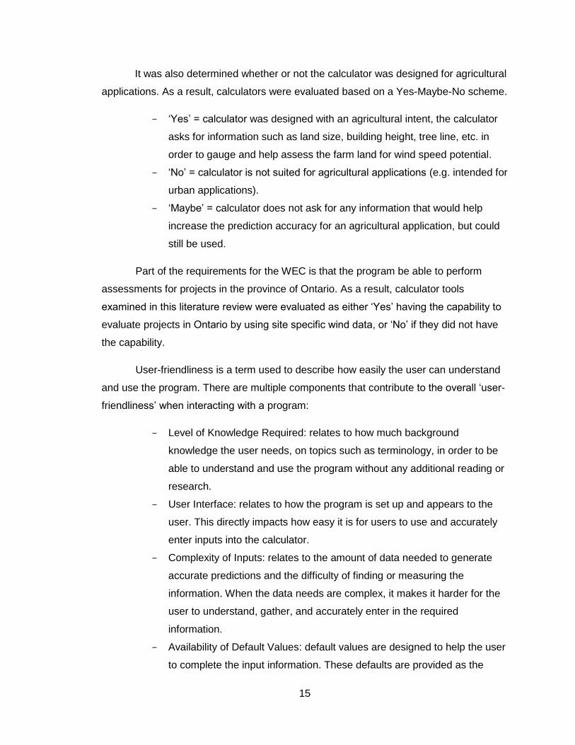
It was also determined whether or not the calculator was designed for agricultural

applications. As a result, calculators were evaluated based on a Yes-Maybe-No scheme.

- ‘Yes’ = calculator was designed with an agricultural intent, the calculator

asks for information such as land size, building height, tree line, etc. in

order to gauge and help assess the farm land for wind speed potential.

- ‘No’ = calculator is not suited for agricultural applications (e.g. intended for

urban applications).

- ‘Maybe’ = calculator does not ask for any information that would help

increase the prediction accuracy for an agricultural application, but could

still be used.

Part of the requirements for the WEC is that the program be able to perform

assessments for projects in the province of Ontario. As a result, calculator tools

examined in this literature review were evaluated as either ‘Yes’ having the capability to

evaluate projects in Ontario by using site specific wind data, or ‘No’ if they did not have

the capability.

User-friendliness is a term used to describe how easily the user can understand

and use the program. There are multiple components that contribute to the overall ‘user-

friendliness’ when interacting with a program:

- Level of Knowledge Required: relates to how much background

knowledge the user needs, on topics such as terminology, in order to be

able to understand and use the program without any additional reading or

research.

- User Interface: relates to how the program is set up and appears to the

user. This directly impacts how easy it is for users to use and accurately

enter inputs into the calculator.

- Complexity of Inputs: relates to the amount of data needed to generate

accurate predictions and the difficulty of finding or measuring the

information. When the data needs are complex, it makes it harder for the

user to understand, gather, and accurately enter in the required

information.

- Availability of Default Values: default values are designed to help the user

to complete the input information. These defaults are provided as the

16

standard, or most common, values so that if the user does not have the

exact information to enter they are able to identify and use an accepted

value instead.

- Level of Supplementary Information: sometimes programs come with a

user manual to help the user with issues they encounter, describe the

calculator methodology and assumptions, etc. This information can assist

the user in working through the program, even if the user is not thoroughly

knowledgeable in the area.

- User-friendliness of Supplementary Information: when additional

information is provided, it should be in a form that is easily accessible and

understandable by the user. Answers to problems should be easy to

locate and the user should then be able to quickly understand and

implement the solution.

All of these components that contribute to the overall level of ‘User-friendliness’ of a

program were evaluated as ‘High’, ‘Moderate’, or ‘Low’. The criteria are structured so

that ‘High’ is the most desirable rating for all criteria.

The quality of predictions provided is a measure of the anticipated accuracy and

reliability the output information of different calculators. Quality depends directly on the

type and quantity of input information required from the user, including site location

information and turbine information. Although asking for a lot of information from the user

can make the calculator more tedious to use, at the same time it allows the calculator to

perform more accurate predictions with the detailed information. The risk of asking a

user for significant amounts of detailed information is that the information may exceed

the user’s level of knowledge. If a lot of information is required, there is an increased

probability that incorrect information will be entered into the calculator. Thus, even

though the information is meant to increase the accuracy of the prediction, the opposite

could happen. Additionally, it is imperative to get detailed information about the user’s

location of interest for the turbine to help gather more precise wind speed data. This

information also provides insight on site features which could present obstacles to wind

flow and hence decrease the productivity of the turbine. As a result, the following

components were assessed as they will contribute to the overall quality of predictions

generated:

17

- Location Information = what information regarding site location is

requested from the user. Asking for detailed information increases the

chance for producing a reliable result, though by no means guarantees it.

- Resource Database = whether the calculator pulls wind speed information

from a resource database or asks the user to enter wind speed data.

- Proximity of Resource Data to Location = with the entered location

information, it can be determined how close to the site the resource data

was taken from. As distance between turbines sites and wind speed data

locations decreases, the wind data has greater ability to be representative

of wind speeds observed at the site of interest. Therefore, if data sites are

far away from the site of interest, it can be assumed that it will not

represent the site wind speeds as accurately.

- Manually Add Resource Data = whether or not the calculator allows the

user to enter in more accurate wind speed information if it is known. Most

individuals will not know how to find wind data or have access to wind

speed data specific to their site of interest. However, if they do, the

reliability of calculator predictions will increase if they are able to manually

input the more accurate wind speed data.

- Wind Speed Model = which model is used to predict wind speed

characteristics. The two common methods the Weibull and Rayleigh

probability distribution models. The Rayleigh distribution is a simplified

version of the Weibull model and has the advantage of being able to

predict probability and cumulative distribution functions from only the

mean wind speed. The Weibull model, however, requires more

information on scale and shape factors but is better at fitting to monthly

wind speed probability distributions and better at providing power density

distributions over the year (Celik 2003, Erlich and Shewarega 2007).

- Calculation Transparency = how much detailed information is provided

describing how calculation are performed. If the user is able to read

through and understand the variables used and the calculations

performed, they can be more confident in the estimates it produces.

18

The overall quality of predictions were evaluated for each calculator based on a ‘High’,

‘Moderate’, and ‘Low’ ranking system, where calculators ranked ‘High’ are anticipated to

produce higher quality and more reliable results.

The economic component of the calculators was evaluated in two parts. First,

and most importantly to the user, was whether or not a financial analysis was performed.

This can include the presentation of payback period or return on investment (ROI).

Payback period is the length of time after turbine installation where the revenue

generated from the turbine pays for the cost of the turbine project (Fraser et al. 2009).

ROI calculates the percentage the lifetime net income is of the initial installation costs.

These features are essential for the user to know whether or not they will gain or lose

money on the wind turbine project. Additionally, calculators were also evaluated as to

whether or not the analysis is as realistic and representative as possible. For results to

be representative they have to take into account several factors including: whether or not

the turbine is connected to the grid, the price electricity is bought or sold for, capital cost

of the project, and how the project is financed (loan amount and interest rate). Both of

these characteristics (financial analysis and realistic assessment) were evaluated on a

‘Yes’ or ‘No’ basis. Calculators ranking ‘Yes’ in both instances provide the type of

economic assessment that the typical user is seeking.

Finally, the ability of the tools to compare different technologies was examined

and is one of the key features of the CEDST program. Evaluation was performed on a

‘Yes’ or ‘No’ system, with tools being able to compare the economics of multiple different

technologies at one time receiving a ‘Yes’ and, conversely, ‘No’ if they were not able to

do so.

A literature review was performed to examine the existing wind energy calculator

tools to determine if there is actually a need for the CEDST WEC project. Assuming the

knowledge level and resources available to a farmer, wind prediction tools analysed

were found by searching online for reputable sources that offer the desired wind

resource assessment services. The web is an excellent place to start research on

renewable energy systems without having to incur the costs of hiring a consultant,

especially for initial assessments. A total of seven wind energy calculators were selected

to be the substance of the literature review based on those readily available and most

frequently used. These tools include:

19

- RETScreen – Natural Resources Canada (Leng et al. 2009)

- HOMER – National Renewable Energy Lab, U.S. Department of Energy

(Lilienthal et al. 2009)

- The Ballpark Cost Calculator ‘CanWEA’– Canadian Wind Energy

Association (CanWEA 2005)

- My Wind Estimator – SolarEstimator.Org (EML 2000)

- Wind Project Calculator – Windustry (Orrell and Antonich 2007)

- Wind Turbine Power and Economics Calculators (2 calculators) ‘DWIA’–

Danish Wind Industry Association (DWIA 2003a, 2003b)

- Small Wind Energy Estimator Tool (Cadmus 2007)

Calculators selected were developed by knowledgeable and reputable

organizations, performed feasibility assessments, and were tools that were widely used

and recommended within the wind industry for site assessment. Additionally, most of

these calculators have a resource database built in so that the user does not have to

search for wind data specific to their location. Of the calculators, two were developed by

Canadian organizations, four by organizations in the United States, and one that was

developed in Europe. The origin of the calculator does not necessarily restrict the

geographic scope of the potential assessment locations, which is why calculators were

evaluated that were not solely developed in Ontario. For example, RETScreen was

developed in Canada and it can handle site assessments across the globe (RI 2012a).

Table 2 outlines results from the evaluation of the seven calculators. A short

summary of each calculator analysis is provided in the following sections.

2.2 Literature – Existing Renewable Energy Calculators

The following sections will explain the reasoning for the results of Table 2 in which each

of the seven calculators were evaluated. Each section that follows will address an

individual calculator.

2.2.1 RETScreen

One of the most widely used and recognized renewable energy calculators across the

globe is RETScreen. RETScreen was developed by the CanmetENERGY of the Natural

Resources Canada (NRCan) (Leng et al. 2009). Development began in 1996 and

produced the Renewable Energy for Remote Communities (RERC) Program. With

20

continued progress of the RERC program over the following years, the program was

renamed in 2004 as RETScreen International Clean Energy Decision Support Centre,

and since has undergone numerous version upgrades to what is currently available

(Leng et al. 2004). RETScreen is available to the public free of charge, and the most

current version, RETScreen 4, is available in 36 languages making it usable to

approximately two thirds of the world’s population (RI 2012b). The climate database

covers the entire planet, including all central, isolated, and off-grid areas (RI 2012b).

With these two features, RETScreen is the only renewable energy (RE) calculator easily

used by people of varying nationalities and for projects anywhere around the globe. As a

result, it is possible to perform wind project assessments across the province of Ontario,

which is the geographic focus of the CEDST application.

RETScreen is an Excel based program, and is designed to produce estimates on

total construction and implementation costs of a user specified wind turbine project. The

user selects location, turbine, and financial information which best describes their project

and RETScreen produces a feasibility assessment including payback period and internal

rate of return (IRR) based on the energy production calculated (Leng et al. 2009). While

the calculator asks the user for basic information on location, wind turbine, and financial

parameters, the user is able to specify the degree of information they wish to provide on

the wind resource and technology. This is done by selecting one of three different

methods within the calculator itself, allowing the user to work in a calculator that best

suits their level of knowledge on the project. Simpler methods use internal default

values, while more complex models allow the user to input specific information

concerning location, resource, wind turbine, and technical details.

While it is good to have this flexibility and to use Excel (which most people would

be familiar with), RETScreen can still be a confusing and overwhelming tool to use as it

is hard to determine where information is needed, how to input the proper information,

and how to model a project on or off the grid, or ones with other financial incentives.

Even though this is the case, there are default values provided for each category so it is

possible to generate a prediction, and the quality of prediction will just be dependent on

the user and their level of knowledge. Overall, users require a basis of knowledge, both

on how to work RETScreen and also on the technical project details, in order to use

RETScreen to make a prediction for a representative project. There are tutorials,

supporting literature, help buttons, and other information available to help guide the user

21

to achieve accurate results (RI 2004a). The supplementary information, however, is

long and detailed and not designed to quickly and concisely address the user’s issues.

Putting all of these factors together indicates that RETScreen is not a highly user-friendly

tool.

If the user was able to utilize RETScreen effectively, wind resource data may still

prove to be barrier to generating a realistic feasibility assessment. The wind resource at

a turbine site dictates the amount of power the turbine will generate, and hence impact

the economics of the project. As a result, if the wind resource information used in a

prediction is not representative of what will be seen at the site of interest then the

feasibility assessment will not be realistic to what the user can expect to see. In the case

of RETScreen, wind speed information is based on a combination of NASA Satellite

Data (RI 2004a), and data from 6,500 surface weather stations across the world (RI

2012b). Users select the city closest to their location and RETScreen draws on its

resource database to pull out wind speed location for that city. While both NASA and

weather stations are fairly reliable sources, the fact that RETScreen does an

assessment for the ‘closest city’ location rather than the exact turbine site means that

the wind data used in the assessment is not necessarily representative of the site of

interest. The significance of this issue will be examined in greater detail in Chapter 11 –

Wind Case Study Analysis of this thesis. RETScreen’s ‘Method 3’ for characterizing wind

speeds does, however, allow a user to manually adjust monthly wind speed information

if more accurate data is available compared to the default information provided.

Additionally, the tool does not take into account any micro-siting information, such as

trees, buildings, etc., that impact wind flow. With this in mind, RETScreen is not

specifically suited for agricultural, rural, or urban applications, but would be utilized in the

same manner for each.

RETScreen utilizes the Weibull distribution for wind speed information (RI

2004a). Additionally, the supplementary material goes over each calculation performed

by the tool in great detail (RI 2004b). With these two features, the user can be confident

in understanding how RETScreen arrives at its predictions and thus can be confident

that the results were produced by robust and reliable methods.

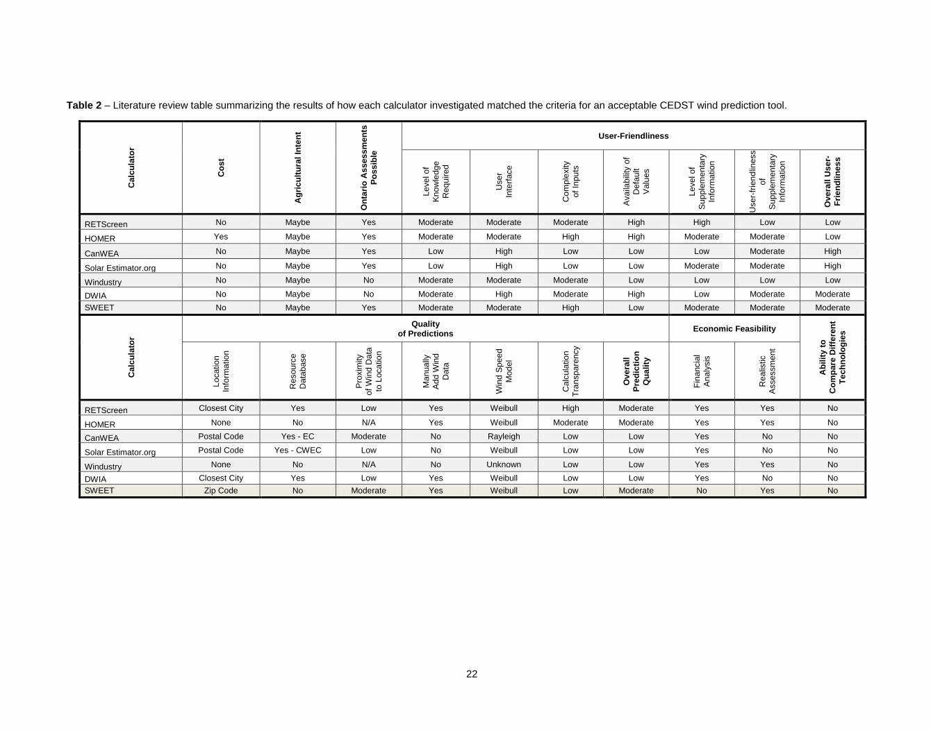
Table 2 – Literature review table summarizing the results of how each calculator investigated matched the criteria for an acceptable CEDST wind prediction tool.

Ca

lcu

lato

r

Co

st

Ag

ric

ult

ura

l In

ten

t

On

tari

o A

ss

ess

men

ts

Po

ss

ible

User-Friendliness

Le

vel o

f

Kn

ow

ledg

e

Re

qu

ired

Use

r

Inte

rface

Co

mp

lexity

of

Inpu

ts

Ava

ilab

ility

of

De

fau

lt

Va

lues

Le

vel o

f

Su

pp

lem

en

tary

Info

rma

tio

n

Use

r-fr

ien

dlin

ess

of

Su

pp

lem

en

tary

Info

rma

tio

n

Ov

era

ll U

se

r-

Fri

en

dli

ne

ss

RETScreen No Maybe Yes Moderate Moderate Moderate High High Low Low

HOMER Yes Maybe Yes Moderate Moderate High High Moderate Moderate Low

CanWEA No Maybe Yes Low High Low Low Low Moderate High

Solar Estimator.org No Maybe Yes Low High Low Low Moderate Moderate High

Windustry No Maybe No Moderate Moderate Moderate Low Low Low Low

DWIA No Maybe No Moderate High Moderate High Low Moderate Moderate

SWEET No Maybe Yes Moderate Moderate High Low Moderate Moderate Moderate

Calc

ula

tor

Quality of Predictions

Economic Feasibility

Ab

ilit

y t

o

Co

mp

are

Dif

fere

nt

Te

ch

no

log

ies

Lo

catio

n

Info

rma

tio

n

Reso

urc

e

Data

base

Pro

xim

ity

of

Win

d D

ata

to L

oca

tio

n

Ma

nua

lly

Ad

d W

ind

Data

Win

d S

pe

ed

Mo

del

Calc

ula

tio

n

Tra

nsp

are

ncy

Ov

era

ll

Pre

dic

tio

n

Qu

ali

ty

Fin

ancia

l

An

aly

sis

Rea

listic

Assessm

en

t

RETScreen Closest City Yes Low Yes Weibull High Moderate Yes Yes No

HOMER None No N/A Yes Weibull Moderate Moderate Yes Yes No

CanWEA Postal Code Yes - EC Moderate No Rayleigh Low Low Yes No No

Solar Estimator.org Postal Code Yes - CWEC Low No Weibull Low Low Yes No No

Windustry None No N/A No Unknown Low Low Yes Yes No

DWIA Closest City Yes Low Yes Weibull Low Low Yes No No

SWEET Zip Code No Moderate Yes Weibull Low Moderate No Yes No

22

23

Economic feasibility results are presented both numerically and graphically in the

program and, if the user is knowledgeable and able to use the program competently,

RETScreen is able to generate assessments which are realistic to what can be expected

for the project in real life.

Overall, RETScreen has the potential to be a fairly representative tool for wind

turbine economics if, and only if, the user is knowledgeable in the area of wind energy

and competent in using the tool. The low user-friendliness of RETScreen, along with the

issues with resource data and not being focused on agricultural applications, prevents

this tool from meeting the requirements of the CEDST project and therefore has room for

research and development to be done to generate a renewable energy (RE) calculator

better suited to those needs. When looking on the entire scope of the CEDST initiatives,

RETScreen also does not have the capability of performing direct comparisons between

RE systems.

2.2.2 HOMER

HOMER, ‘Hybrid Optimization Model for Electric Renewables’, is the most prominent RE

assessment tool coming out of the United States (Lilienthal et al. 2009) and as such is a

competitor to RETScreen. Being on similar level of RETScreen, HOMER was actually

used to validate the results of specific cases generated by RETScreen (RI 2004a). While

the calculators are somewhat comparable, HOMER is also distinctly different. This tool

allows users to look at hybrid power systems that may be created from RE generators

and battery technologies (HE 2011), though a hybrid system is still not the technology

comparison desired for the CEDST application. Additionally, HOMER is an executable

software program (i.e. not Excel) that must be downloaded by the user and comes with a

licensing cost of $198 USD/year for the most up-to-date versions of the program,

although older versions can be accessed for free (HD 2012). For the purposes of this

research HOMER 2.68, released July 24, 2009, was evaluated. This program is the most

recent version of HOMER available that can be downloaded without having to pay the

licensing fee, even though there have been an additional 5 versions created which have

included numerous updates and improvements over HOMER 2.68 (HVH 2012). While

HOMER 2.68 is not the most up-to-date version of the program available, it does

realistically represent the program that a farmer would choose to use for a wind site

assessment because an individual seeking a one-time assessment would unlikely pay

for the licensed version of the program.

24

HOMER 2.68 is not designed specifically for agricultural applications, but does

have the ability to perform an agricultural site assessment which can be done for most

locations, including Ontario. HOMER, similar to RETScreen, requires the user to have

knowledge of RE systems and to be familiar with using the calculator in order to be

successful in producing results. This is because it is not intuitive how to use HOMER, it

is not formatted with a clear progression to enter data, it is hard to identify where data

needs to be entered, the help provided is not very effective, many complex inputs are

required, and the results are extremely hard to interpret for an untrained individual.

Although there are default values and supplementary information provided, they are not

effective at helping the user enter correct information or use the program. As a result,

the calculator is not user-friendly.

Looking into the structure of the calculator, there is no wind resource database

built into the program and therefore the individual is required to find and enter the wind

speeds for their location of interest. While this means that the wind data will be more

accurate to the site of interest (depending on where or how the data was obtained) it

also means that the user must find that data. HOMER uses a Weibull wind speed

probability distribution (Lambert et al. 2006) and is transparent with some, but not all, of

the calculations. The overall prediction quality of HOMER 2.68 was evaluated to be ‘Low’

due to the fact that this calculator is extremely hard for a user without much RE

experience to use and generated results. There is the possibility of generating a financial

analysis of the project which is fairly realistic to what could be expected, but the only way

to achieve that is through having an strong knowledge of RE and HOMER.

In summary, HOMER 2.68 is not a user-friendly tool, is not designed for

agricultural site assessments, and does not have the capability of performing

comparisons between technologies. As a result, this tool does not fulfill the needs of the

CEDST project.

2.2.3 CanWEA: Ballpark Cost Calculator

Another Canadian-made calculator is the Ballpark Cost Calculator designed by the

Canadian Wind energy Association (CanWEA) (CanWEA 2005). This calculator is based

online and is designed specifically for small turbine evaluation (CanWEA 2005), which is

the target technology size of the CEDST project. It is much simpler to use, when

compared to RETScreen or HOMER, in that the data required is minimal, simplistic and,

25

in most cases, common knowledge (e.g. postal code, utility region, monthly electricity

bill, etc.). Results are clearly presented and focus only on the most important aspects of

an economic assessment: capital and installation costs, energy output, and simple

payback period (CanWEA 2005).

With this information, the calculator pulls from the Environment Canada

Canadian Wind Energy Atlas database (CanWEA 2010a) to get wind speed information.

The Canadian Wind Energy Atlas it a reputable source and provides detailed wind data,

at varying heights, for over 300,000 locations in Ontario (CWEA 2003a), but CanWEA

does not detail how it uses the postal code to obtain wind speed data for its predictions.

Additionally, even though CanWEA uses the RETScreen methodology for behind the

scenes calculations (CanWEA 2005), it makes many simplifying assumptions that impact

the overall reliability of results presented. For example, it uses a Rayleigh wind speed

probability distribution as opposed to the more accurate and complex Weibull distribution

(CanWEA 2010a). As well, it is assumed that electricity is being bought and sold to the

grid at the same rate, which fails to take into account the incentives being offered in

Ontario for renewable power generation (CanWEA 2005). Failing to take into account

local wind effects, accurate modelling, and accurate economic parameters decreases

the accuracy and reliability of the results provided.

Although these simplifications impact the overall prediction quality, they do limit

the amount of detailed information that the user is required to share and increase the

usability and user-friendliness of the calculator. Similar to both HOMER and RETScreen,

the CanWEA Ballpark Cost Calculator is not designed specifically for agricultural

applications and also does not have the capability to compare different technologies.

Bringing all of these features together indicates that although the CanWEA Ballpark Cost

Calculator is very easy to use, its shortcomings and missing elements do not make it

well suited for the CEDST project.

2.2.4 Solar Estimator.org: My Solar & Wind Estimator

My Solar & Wind Estimator was developed by the US company Energy Matters LLC. for

the purpose of providing solar photovoltaic and wind turbine site assessments (EML

2000). It is similar to the Canadian CanWEA Calculator in that it is an online, user-

friendly wind assessment tool (EML 2000). Basic inputs of zip or postal code, monthly

energy bill, and power supplier are all that is required to generate a basic assessment

26

and the user has the option of performing an assessment for a wind turbine or solar PV

system, but not both simultaneously. This calculator is better designed then CanWEA as

it allows the user to more easily change variables to better represent the project (e.g.

grid system, electricity rate, project cost, loan amount, income tax, etc.) and terms,

assumptions, and models are well defined. As well, it also presents economic feasibility

results in an easy to understand manner in both numerical and graphical formats.

While the simplicity makes the calculator very easy to use, there are also

downsides as well. Wind data is obtained either from the NASA or Canadian Weather for

Energy Calculations (CWEC) database for US and Canadian locations, respectively. The

CWEC data is for 75 locations across Canada and, using the latitude and longitude

derived from the postal code entered in by the user, the calculator takes the site location

and uses the closest CWEC data for calculations (EML 2012). As such, the CWEC data

used does not necessarily accurately describe the wind resource at the location of

interest. As well, simplicity of inputs used in this calculator means that the prediction is

dependent to the generic default values used within the program, rather than, for

example, allowing the user to pick a specific wind turbine model. Lack of agricultural,

micro-siting features and inability to compare different technologies to the wind turbine

assessment in addition to the other factors described, make this calculator insufficient to

fulfill the needs of the CEDST project.

2.2.5 Windustry: Wind Project Calculator (WPC)

Windustry, an American based organization, has produced a wind resource assessment

tool which is available for download by the public and free of charge (Orrell and Antonich

2007). Similar to RETScreen, the Wind Project Calculator (WPC) is based in Excel,

although it utilizes many different worksheets in the program where RETScreen more

simply utilizes one worksheet to do a wind feasibility assessment (Orrell and Antonich

2007). Even though individual worksheets are dedicated to a specific component of the

assessment, the sheer volume of worksheets makes it very hard to identify the inputs

required, follow calculations, relate worksheets to one another, distinguish conclusions,

and identify the overall feasibility of the proposed project. The WPC does not perform a

site assessment, nor does it look at agriculture specifically, but rather uses assumptions

and minimal user inputted values to perform an economical evaluation of the project.

This requires the user to enter the program with a strong knowledge of wind energy

technology and the amount of energy a turbine would produce at the site of interest.

27

Additionally, there is little to no supplementary information available on the program

which makes it very hard for a new user to learn to use the program and also to

understand models used and the calculations that go on internally. Although WPC does

produce a feasibility assessment, it is hard not only to interpret the results, but also to

achieve an accurate model of the project of interest.

To summarize the Windustry WPC features, it is not user-friendly for a novice

user, has questionable prediction quality since it does not perform a site specific

assessment, and does not have documentation that clearly details how calculations are

performed. These characteristics, coupled with the fact that it is unable to perform a

comparison between different RE technologies, makes the WPC not suitable for the

CEDST application.

2.2.6 DWIA: Wind Power and Economics Calculators

The Danish Wind Industry Association (DWIA) has developed two calculators that can

be utilized together to perform a wind assessment. DWIA has a Wind Turbine Power

Calculator (WTPC) and Wind Energy Economics Calculator (WEEC) which are used to

predict power generated by a turbine and the economics of a wind project respectively

(DWIA 2003a, 2003b). Each calculator is available to the public via the DWIA website

and the WTPC contains wind data for cities in European countries including: Germany,

Italy, and the Netherlands (DWIA 2003a). The user selects the closest city to their

location of interest from a drop down list and then the WTPC uploads the respective

wind and climate data from the European Wind Atlas database (DWIA 2003a). While the

wind database is limited to select cities, the user maintains the ability to input more

accurate wind data. As such, even though the calculator is designed for European use,

the user would still be able to generate a prediction for Ontario if the correct wind and

climate data was known. Additionally, there is no specific agricultural characteristics built

into the calculator but it could be utilized to roughly model such projects. Using a Weibull

distribution for wind speed, along with information regarding the specific turbine that the

user selects from a drop down list, the WTPC generates turbine power output results

(DWIA 2003a). The WTPC is fairly easy to use right from the first time a user attempts a

power assessment with prediction results well presented. Aside from identifying the wind

probability distribution model, supplementary information provided by the calculator is

limited and makes it hard to understand how the wind power calculations are performed.

28

Taking the information produced by the WTPC and entering it into the WEEC,

along with some basic cost and investment details, the WEEC produces a Net Present

Value (NPV) and Real Rate of Return (RRR) of the wind project (DWIA 2003b).

Opposed to providing a payback period, the feasibility of the project is determined by

interpreting the predicted NPV and RRR, with positive NPV values meaning that the user

can expect to gain money from the investment and the RRR percentage dictating the

return anticipated on the investment. Similar to the WTPC, the WEEC is easy to use but

is harder to manipulate to accurately model the specific project of interest and it does not

have detailed supporting documentation to explain how calculations are performed.

In the case of WTPC and WEEC, both calculators are needed to produce a

feasibility assessment, but it is not difficult to do so as both are fairly user-friendly. The

quality of predictions for the calculators is low since very limited project inputs are

required and thus it is hard to form a realistic model of the project. Additionally, the

calculators are designed specifically to evaluate wind turbines and do not have the ability

to compare turbines to different RE technologies. All in all, the DWIA calculators are

unable to fulfill the requirements of the CEDST program.

2.2.7 Cadmus: Small Wind Energy Estimator Tool (SWEET)

The Cadmus Group, in conjunction with the Massachusetts Renewable Energy Trust

(MRET), developed the Small Wind Energy Estimator Tool (SWEET) in 2007. SWEET is

an Excel-based program that uses three steps to generate a wind prediction. Version 1

of the tool was analyzed. Although a newer version was said to be available (Shaw et al.

2008) it was not readily found or accessible to the public.

The tool started by asking for turbine, site, and wind information. Turbine models

are provided in a drop down menu but it is hard to determine the power rating of the

turbines. It is possible to enter in information for other turbines but the user would have

to know the technical details. Site information is requested in the form of latitude and

longitude coordinates which would then be used by the user to manually find the site

wind speed. The issue that arises for Canadian location is that the links provided, if they

work at all, are only valid for sites in the United States. Though, if the user was

resourceful and could find the information themselves they would still be able to use the

program. Detailed information is then requested on the wind speed frequency and terrain

type in all directions surrounding the site of interest. Wind speed frequency is incredibly

29

detailed information that, if not provided by a resource database, a user would not be

able to provide. The final step provides a summary and states whether the turbine is

valid or not under the Massachusetts subsidy program. As a result, it is not possible to

generate a feasibility assessment using the Ontario FIT guidelines.

Overall the calculator is fairly easy to use, although the information asked for is

not easily found and the program is not suited for generating Ontario wind feasibility

assessments. The quality and reliability of results is questionable as the information

available explaining the program is very limited and does not concisely describe the

calculator methodology. SWEET is designed to only evaluate a single turbine at a time

and does not possess the ability to assess multiple turbines or provide a comparison

between different renewable energy technologies. Therefore, after examining the

SWEET model for wind turbine assessment, the tool does not fulfill the requirements of

the CEDST project.

2.3 Literature Review Conclusions

After analyzing different wind energy calculators, it is apparent that there is a wide range

of wind resource assessment options available to an individual seeking to evaluate the

economic potential of a wind turbine project.

Simpler, easier to use calculators, including CanWEA, SolareEstimator.org, and

DWIA, come with a price of decreased quality and reliability of predictions. This is due to

the fact that simpler calculators generally make assumptions internally within the

program to compensate for less user inputted information and also are not accompanied

by sufficient supporting literature to instill confidence in the user that calculations are

performed accurately. Simplifying assumptions, such as with CanWEA where electricity

is bought and sold at the same rate, can severely impact the predicted feasibility of a

project and may lead the user to conclusions which are not accurate. While the results

produced are not necessarily a good representation of what can be expected from the

project, the user-friendliness of the calculators makes them very appealing and easy to

use by individuals with limited wind energy knowledge.

In contrast, while calculators like RETScreen, HOMER, SWEET, and Windustry

are more complex and complicated to use, they possess the potential to generate more

accurate and representative economic assessments. Having more detailed project

30

information, these calculators can utilize details specific to the project of interest to

perform calculations rather than relying on default values or assumptions like the simpler

calculators. In and of itself, the level of specific technical knowledge required for these

calculators make them extremely un-user-friendly, as it makes users who do not have

this knowledge confused, overwhelmed, and more likely to input unrealistic information.

Additionally, these calculator interfaces are harder to use and identify where inputs are

required and, though they may come with supporting literature to aid the user in going

through the calculator, the literature is not in effective or efficient forms.

It was also observed that no calculators, whether simple or complex, are

designed specifically to take agricultural site features into account, such as barns,

treelines, or buildings, nor did any possess the ability to take the wind feasibility

prediction and compare the results to the feasibility of other green technology projects.

Overall, the review of the existing wind energy assessment tools revealed that

both simplistic, user-friendly calculators and also detailed, complex calculators have

problems in generating realistic and reliable feasibility predictions. The potential quality

and reliability of predictions also appears to have an inverse relationship with user-

friendliness; as user-friendliness increases, the overall accuracy and confidence in

predictions decreases. As well, no calculators exist that are able to fulfill the two most

important CEDST project goals: of being agriculturally focused and having the ability to

compare the feasibility of multiple different green energy projects.

2.4 Literature Review Implications

This literature review of existing wind energy assessment tools found that there are no

calculators currently available that encompass all of the features, as outlined in Section

2.1, desired for the wind energy module of the CEDST. As a result, there are many

improvements that need to be made in order to develop the CEDST Wind Energy

Calculator (WEC) into a suitable program that can be implemented into the greater

CEDST program.

In order to incorporate agricultural siting into the WEC, factors such as land size,

terrain type, tree lines, and buildings need to be identified. Having this information is

important because it will allow for appropriate variables to be used in calculations which

most accurately model the land surface that the wind is flowing over. Additionally, having

31

information about tree line and building locations can allow the WEC to help the farmer

identify optimal locations for the turbine (effectively micro-siting the turbine). Including

these micro-siting components will help calculate the most accurate wind speed data

and thus help give an optimal prediction.

To improve upon the wind speed data used for the assessment, the WEC should

use more location specific information than that available by postal code region or

closest city approximations. An option to do so would be to have data for wind speeds

across Ontario and then obtain site specific measurements based on geographical

coordinates (longitude and latitude). This will be possible through the incorporation of

Google Earth into CEDST, through which the farmer will be able to highlight the

locations of property boundaries and then Google will be able to pull the corresponding

geographical location.

Additionally, it is apparent that there is a need for accurate and reliable

assessments of wind turbine feasibility. In order to achieve this from a user-operated

tool, there needs to be an optimum balance between user-friendliness and complexity.

The WEC must be easy enough for a farmer, who does not have a significant renewable

energy background, to use but also be able to gather and utilize project specific data in

order to generate a realistic model for the project. This could come in the form of the

user being able to select and enter data that most accurately describes the project, but

not requiring data beyond a reasonable scope of knowledge. Drop down menus,

databases of information, default values, and explanations of variables will help in

achieving this objective. Minimizing inputs maintains user-friendliness, while educating

the user will help ensure that the correct value will be entered into the program.

One way to minimize the inputs required in the WEC would be to evaluate,

understand and streamline the decision making process. The decision making process

(DMP) for a wind assessment involves looking at all of the information and costs that go

into installing, commissioning, and operating a wind turbine. These decisions include:

deciding the size and type of turbine to install, choosing a location that optimizes energy

production, whether to connect to the grid, predicting maintenance costs, etc. If these

decisions can be broken down into steps, project specific information can be

differentiated from other information that can reasonably be approximated from industry

32

averages and thus will help streamline the inputs needed for the WEC to be an effective

assessment tool.

A final component that needs to be included into the WEC is ensuring that the

economic results generated are not only realistic, but also easy to interpret and easy to

quickly draw comparisons between other green technology assessments. Economic

assessments will be presented numerically and graphically in the final CEDST program.

The goal of CEDST is that a farmer will be able to simultaneously assess the economics

of different green energy technologies. In order to do so, the economics of the

technologies must be easy to interpret, compare, and identify the best options. The WEC

must generate a concise, but accurate and descriptive, evaluation of wind turbine

feasibility.

33

Chapter 3 – Decision Making Process

3.1 Existing Models

The previous sections have set the stage for the development of the CEDST Wind

Energy Calculator (WEC). The aim of this research was presented, the specific goals of

the WEC, as well as overall CEDST project, have been identified, and a review of

existing renewable energy (RE) decision support tools revealed that there is no tool

currently available that fulfills those goals. As a result, it has become clear that effort

needs to be focused on developing the WEC to meet the CEDST objectives.

What the WEC is trying to achieve can be summarized as follows; the WEC will

be a tool designed to create a feasibility assessment of a user defined wind turbine

project that can be easily compared against assessments of other green energy

technologies. The wind project evaluation must be designed for agricultural applications

in Ontario, be user-friendly, and produce reliable results. As such, the WEC must be

able to collect information regarding property size, geographical location, turbine model

of interest, finances, etc. and use the information in a sequence of calculations that

calculate the projected project economics.

A good overview of the entire wind turbine development process is provided by

the American Wind Energy Association in their “10 Steps to Developing a Wind Farm”

(AWEA 2009). The steps are provided as follows:

1. Understand the wind resources

2. Examine existing transmission lines

3. Ensure access to land

4. Obtain required capital

5. Determine power purchaser

6. Examine project feasibility and siting

7. Understand wind economics

8. Permitting and zoning

9. Review potential turbine manufacturers and project developers

10. Plan for annual operation and maintenance requirements

34

This list (AWEA 2009) provides a good overview of the components that need to be

taken into consideration during the decision making process and any good energy

calculator will incorporate most, if not all, of these aspects.

There are different decision making models available that aid in assessing the

wind potential of a site based on all of the above criteria. One such example is the “Multi-

Criteria Decision-Making Model” (MCDM) developed by Lee et al. (2009). The MCDM

uses an analytic hierarchy process (AHP) to rank the different criteria. This hierarchy is

broken up into four categories: ‘Benefits, Opportunities, Costs and Risks’ (BOCR) (Lee

et al. 2009). These categories contain all of the necessary criteria for generating an

effective wind energy project assessment, as seen in Table 3. Each criterion is given a

numerical value representing its level of importance among all criteria in that field,

producing a matrix of ranked values, and the rankings are then multiplied against a

decision vector to get a total numerical score of the wind development potential at a

given site (Lee et al. 2009). Higher scores indicate sites with greater wind energy

development potential.

A different approach by Voivontas et al. (1998) uses a Geographic Information

System (GIS) Decision Support System (DSS) to evaluate the renewable energy

potential of a site and incorporate the spatial interaction between geographic objects

(Voivontas et al. 1998). The renewable energy potential of a site is broken down into four

components for ease of evaluation: theoretical, available, technological, and economic

potential. First, the theoretical potential is estimated, which represents the maximum

amount of energy that a location can offer (Voivontas et al. 1998). Next, geographic and

environmental constraints which may influence the location of a wind turbine, such as

steep slopes, nearby towns or airports, are each examined in order to determine the

available potential of the site (Voivontas et al. 1998). Finally, the technological and

economic potentials of the site are found by determining what portion of the theoretical

maximum energy can be harvested by current turbine technologies and determining the

infrastructure, construction, and technical costs of the project (Voivontas et al. 1998).

The overall process for the Renewable Energy Sources (RES) – Decision Support

System (DSS) is illustrated in Figure 1. The RES-DSS approach is one of the only

decision making models to incorporate local, site-specific geographical considerations

into the evaluation.

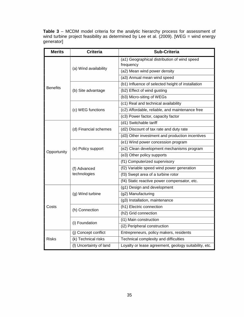
35

Table 3 – MCDM model criteria for the analytic hierarchy process for assessment of wind turbine project feasibility as determined by Lee et al. (2009). [WEG = wind energy generator]

Merits Criteria Sub-Criteria

Benefits

(a) Wind availability

(a1) Geographical distribution of wind speed

frequency

(a2) Mean wind power density

(a3) Annual mean wind speed

(b) Site advantage

(b1) Influence of selected height of installation

(b2) Effect of wind gusting

(b3) Micro-siting of WEGs

(c) WEG functions

(c1) Real and technical availability

(c2) Affordable, reliable, and maintenance free

(c3) Power factor, capacity factor

Opportunity

(d) Financial schemes

(d1) Switchable tariff

(d2) Discount of tax rate and duty rate

(d3) Other investment and production incentives

(e) Policy support

(e1) Wind power concession program

(e2) Clean development mechanisms program

(e3) Other policy supports

(f) Advanced

technologies

(f1) Computerized supervisory

(f2) Variable speed wind power generation

(f3) Swept area of a turbine rotor

(f4) Static reactive power compensator, etc.

Costs

(g) Wind turbine

(g1) Design and development

(g2) Manufacturing

(g3) Installation, maintenance

(h) Connection (h1) Electric connection

(h2) Grid connection

(i) Foundation (i1) Main construction

(i2) Peripheral construction

Risks

(j) Concept conflict Entrepreneurs, policy makers, residents

(k) Technical risks Technical complexity and difficulties

(l) Uncertainty of land Loyalty or lease agreement, geology suitability, etc.

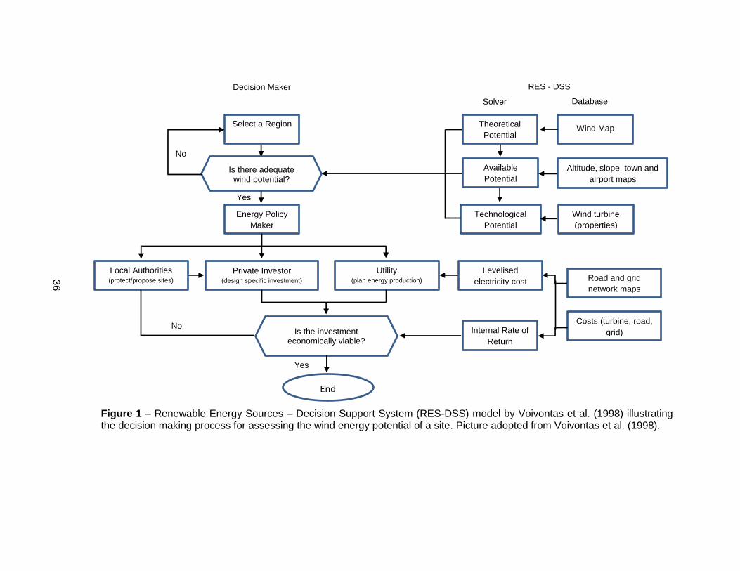
Figure 1 – Renewable Energy Sources – Decision Support System (RES-DSS) model by Voivontas et al. (1998) illustrating the decision making process for assessing the wind energy potential of a site. Picture adopted from Voivontas et al. (1998).

Select a Region

Energy Policy

Maker

Local Authorities (protect/propose sites)

Private Investor (design specific investment)

Utility (plan energy production)

Is there adequate wind potential?

Is the investment economically viable?

End

Theoretical

Potential Wind Map

Altitude, slope, town and

airport maps

Available

Potential

Wind turbine

(properties)

Technological

Potential

Levelised

electricity cost

Costs (turbine, road,

grid)

Road and grid

network maps

Internal Rate of

Return

No

No

Yes

Yes

Decision Maker RES - DSS

Solver Database

36

37

As these three examples illustrate, there are many different ways to organize the

decision making process associated with the assessment of wind energy generation

potential at a site.

The American Wind Energy Association (AWEA 2009) provides a good overview

of the factors that need to be considered when performing such an assessment, though

the list is not exhaustive. As an overview, this can be built upon to create a solid decision

making framework for the WEC.

Lee et al. (2009) produced an interesting interpretation of how to decide whether

or not to install a wind turbine. While this model provides more detail then AWEA, the

assessment is based more on deciding how to rank a feature then actually utilizing a

value to perform calculations and produce numerical results. This type of decision

scheme is complex and not ideally suited to be transcribed into a calculator format,

although the criteria are useful in identifying elements to incorporate into the calculator.

Voivontas et al. (1998) provided the best combination of detail and structure that

could be transcribed into a calculator. Each box in the map represents a piece of

information that comes into play when making the overall decision as to whether or not

the investment is economically viable. The visual illustration helps convey how data is

interrelated and helps communicate the sequence of required data (for example, wind

map data is needed before being able to assess the theoretical potential of a turbine).

Elements of all three models were used to create the structure for the WEC

decision making model, but features were added, removed, or modified to more

accurately reflect the information required for wind project decision making in Ontario.

3.2 Wind Energy Calculator (WEC) Decision Making Model

Based on these three models, the decision making process for the WEC will be laid out

in both list and visual form and will be based on calculations, rather than the analytic

hierarchy process, to produce results to form the basis for an overall feasibility decision.

Wind speed characteristics for the location of interest are extremely important

and must be determined at the start of the decision making process. Additionally, since

38

wind speed is not the only factor impacting power and economic calculations, the hub

height, rated power of the turbine, turbine characteristics, and equipment cost must all

be taken into account (Andrews and Jelley 2007). While the equipment cost varies

significantly with turbine size, other aspects including construction, operation and

maintenance (O&M), and electrical connection do not scale proportionally (Lee et al.

2009). This can be understood through the example of laying an electrical connection

between the turbine and the grid. In all cases, no matter the size of the turbine, trenches

must be dug and electrical wiring must be laid to link the turbine and grid. Both small and

large turbines need this feature with the only things that changes being the carrying

capacity of the wiring and width of the trenches: both costs of which do not increase

proportionally with increased size. As a result, one of the most critical steps in deciding

whether or not to install a wind turbine is gathering accurate information on wind speed

data, location, and wind turbine specifications.

While each turbine site is unique, the evaluation of any project’s viability involves

the collection of similar information from site to site and requires a structured decision

making process.

Using the information provided from AWEA (2009), Lee et al. (2009), and

Voivontas et al. (1998), the following steps must be incorporated into the decision

making process for a wind turbine project:

1. Determine latitude and longitude of potential wind turbine site

2. Gather wind speed data for location (using site latitude and longitude) of

interest from a wind speed database

3. Gather information about site: size of property, land use, tree lines,

building locations, etc. This information will be used for determining

calculation parameters and also for micro-siting the turbine.

4. Using location information, determine the distance to the closest grid

connections.

5. Select turbine model, size, properties (including loss coefficients and

power curve) and tower height

6. Use information in 3 and 5 to calculate projected power output of the wind

turbine

7. Determine desired connection type – On Grid / Net Meter

39

8. Determine electricity FIT rate for On Grid system, and electricity purchase

for consumers for the Net Meter scenario

9. Using information in step 5, predict the costs for: turbine equipment and

construction, grid connection, licensing and permitting (OPA), operation

and maintenance (O&M), etc. and generate an overall project cost

10. Using information from steps 6 and 8, calculate the expected revenue or

savings from an On Grid or Net Meter turbine respectively

11. Gather information regarding project financing including: required loan

amount, loan period, interest rate, and compounding period

12. Using the information in 11, calculate the loan payment

13. Use the information calculated in 9, 10 and 12 to generate: a cash flow

graph, projected payback period, and return on investment (ROI) for the

project.

14. Using the information presented in step 13, decide whether the wind

turbine project is feasible or not

The goal of the WEC is only to advise and direct the user as to whether or not

the wind turbine project would be economically feasible. As a result, this decision making

process is used as a first step to determine whether to follow through with more research

and submit applications and permitting requests.

The steps above were translated into a flow diagram as illustrated in Figure 2.

This diagram shows the interrelationship between information and steps. Creating this

diagram provided an opportunity to think about each step, the pertinent information,

where that information has to be accessed from, and the sequence that the steps are

performed in. The flow diagram was organized in such a way that going down the rows

represents the sequence of events that the overall WEC will perform. The first step

requires the user to input information about the project. Taking this information, the WEC

will then pull from its internal databases the necessary data which correlates to the

information specified by the user. With the information and data, the WEC will then go

through a sequence of calculations until it arrives at overall results to present to the user.

This represents the end of the WEC operations and the remaining steps represent the

decisions that need to be made by the user based on the results presented by the WEC,

and then the pursuant steps to be followed depending on the outcome of the decision.

40

Additionally, activities within the flow diagram were categorized as to the activity

type to communicate the source of the information. Green events are representative of

those that require direct information and decisions from the user. Grey boxes correlate to

events where the WEC must pull information from internal databases. Similarly, yellow is

representative of events where the WEC must perform calculations internally within the

program. Finally, the red events are those that must be made by the user based on the

results generated by the calculator. In doing this, the level of involvement by the user

has been highlighted and simultaneously the information required from the user has

been identified. Information and decisions from the user are only required at the

beginning and end of the decision flow model. In the same way, this decision flow model

has also identified the spaces that the WEC must occupy, such as: having reliable

databases of information, being able to perform technical and financial calculations, and

being able to present results to the user.

Overall, the WEC flow diagram presented in Figure 2 is a realistic decision

making framework that incorporates elements from all the wind project decision models

evaluated, and can be directly translated into a skeleton for the calculator.

Figure 2 – Decision making model for the WEC.

41

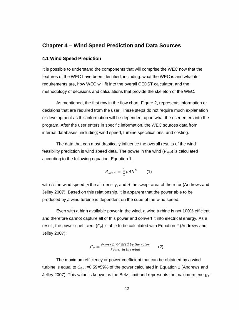
42

Chapter 4 – Wind Speed Prediction and Data Sources

4.1 Wind Speed Prediction

It is possible to understand the components that will comprise the WEC now that the

features of the WEC have been identified, including: what the WEC is and what its

requirements are, how WEC will fit into the overall CEDST calculator, and the

methodology of decisions and calculations that provide the skeleton of the WEC.

As mentioned, the first row in the flow chart, Figure 2, represents information or

decisions that are required from the user. These steps do not require much explanation

or development as this information will be dependent upon what the user enters into the

program. After the user enters in specific information, the WEC sources data from

internal databases, including; wind speed, turbine specifications, and costing.

The data that can most drastically influence the overall results of the wind

feasibility prediction is wind speed data. The power in the wind (Pwind) is calculated

according to the following equation, Equation 1,

(1)

with U the wind speed, ρ the air density, and A the swept area of the rotor (Andrews and

Jelley 2007). Based on this relationship, it is apparent that the power able to be

produced by a wind turbine is dependent on the cube of the wind speed.

Even with a high available power in the wind, a wind turbine is not 100% efficient

and therefore cannot capture all of this power and convert it into electrical energy. As a

result, the power coefficient (CP) is able to be calculated with Equation 2 (Andrews and

Jelley 2007):

(2)

The maximum efficiency or power coefficient that can be obtained by a wind

turbine is equal to CPmax=0.59=59% of the power calculated in Equation 1 (Andrews and

Jelley 2007). This value is known as the Betz Limit and represents the maximum energy

43

that any wind power device can extract from the wind if it were completely efficient.

Generally, modern-day, 3 bladed wind turbines have CP values around approximately

33% (Andrews and Jelley 2007), though this can vary with turbine size and model. It is

then possible to calculate the maximum power of a turbine according to Equation 3

(Andrews and Jelley 2007):

(3)

With the cubic relationship between power production and wind speed, small

changes in mean wind speed can greatly impact the predicted power output of the wind

turbine. It is thus extremely important to predict the wind speed at the turbine site with as

much accuracy as possible. If there is insufficient wind at a given site, a project will not

be an economically sound decision. As a general guideline, which will not hold true for

all cases, mean annual wind speeds of 4.0 - 4.5 m/s are necessary for a wind turbine

project to be feasible (Clarke 2003, RI 2004b). Sites with high average wind speeds

have a greater potential to host an economically feasible wind turbine project.

The most accurate and reliable way to characterize the wind speed at a site is to

measure it directly. If the wind speeds are measured at the exact location where the

wind turbine would be built, the data gathered would take into account all macro and

micro scale features of the property and climate. These features have a direct impact on

wind speed during the time period of the measurement campaign. Measurements of

wind speed, and potentially direction, are gathered by placing anemometers on a tall

tower and hooking them up to a data logger to record the wind data at different heights

(CanWEA 2006b).

While this represents the best way for gathering wind speed data, directly

measuring wind speed is a very financially and time consuming process. To gather

sufficient information it is generally recommend to record wind speeds for at least one

year so that all seasons are represented in the data collected (CanWEA 2006b). Setting

up a tower to measure wind speeds can cost tens of thousands of dollars (NWCE

[N.D]a). A farmer wishing to assess whether a small wind turbine would be a financially

sound may not have the time and funds available to undertake a full wind speed study.

44

4.2 Wind Speed Data

Individuals using the WEC program will most likely not have accurate wind speed

measurements for their site of interest. Therefore the WEC must be able to provide that

information based on external sources. Ideal wind speed data would:

- Be recorded over many years to encompass many different weather

patterns

- Include data from recent years

- Have a high geographical resolution (higher resolution gives better site

specific data)

- Be available as daily (preferably) or monthly wind speed averages

- Be available at different heights

- Have been proven to be reliable and accurate

- Provide coverage across Ontario

In Canada, there are multiple different sources of wind data. The data can be in

the form of wind maps, interactive programs, or downloadable data. There were a

multitude of different sources available for Canadian locations, including: the Canadian

Wind Energy Atlas (CWEA 2003a), Prince Edward Island Wind Atlas (Gasset et al.

2005), New Brunswick Wind Atlas (NBDoE [N.D.]), Environment Canada surface station

data (EC 2012a), NASA (NASA 2012a) and the Ontario Renewable Energy Atlas (OREA

2011a). For Ontario specifically, there were four sources available: the Canadian Wind

Energy Atlas (CWEA), Ontario Renewable Energy Atlas (OREA), Environment Canada

(EC), and NASA. As a result, focus was placed on these four sources and they were

evaluated to assess the suitability for the WEC. Table 4 summarizes the characteristics

of each data source.

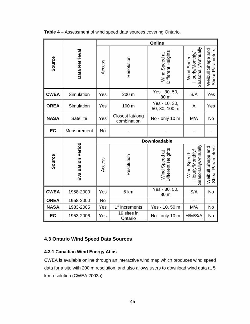
45

Table 4 – Assessment of wind speed data sources covering Ontario.

So

urc

e

Da

ta R

etr

ieval

Online

Acce

ss

Re

solu

tion

Win

d S

pee

d a

t

Diffe

rent

He

ights

Win

d S

pee

d:

Ho

urly/M

onth

ly/

Se

aso

na

lly/A

nnu

ally

We

ibull

Sh

ap

e a

nd

Sh

ea

r P

ara

me

ters

CWEA Simulation Yes 200 m Yes - 30, 50,

80 m S/A Yes

OREA Simulation Yes 100 m Yes - 10, 30, 50, 80, 100 m

A Yes

NASA Satellite Yes Closest lat/long

combination No - only 10 m M/A No

EC Measurement No - - - -

So

urc

e

Ev

alu

ati

on

Pe

rio

d Downloadable

Acce

ss

Re

solu

tion

Win

d S

pee

d a

t

Diffe

rent

He

ights

Win

d S

pee

d:

Ho

urly/M

onth

ly/

Se

aso

na

lly/A

nnu

ally

We

ibull

Sh

ap

e a

nd

Sh

ea

r P

ara

me

ters

CWEA 1958-2000 Yes 5 km Yes - 30, 50,

80 m S/A No

OREA 1958-2000 No - - - -

NASA 1983-2005 Yes 1° increments Yes - 10, 50 m M/A No

EC 1953-2006 Yes 19 sites in

Ontario No - only 10 m H/M/S/A No

4.3 Ontario Wind Speed Data Sources

4.3.1 Canadian Wind Energy Atlas

CWEA is available online through an interactive wind map which produces wind speed

data for a site with 200 m resolution, and also allows users to download wind data at 5

km resolution (CWEA 2003a).

46

This atlas presents data obtained by running atmospheric and environmental

simulations using the Wind Energy Simulation Toolkit (WEST) model. WEST uses a

meso-scale ‘MC2’ model (Benoit 1997) to generate wind data at 5 km resolution and

then, for the CWEA online maps, further refines the data using a micro-scale model

‘MSMicro’ to generate wind predictions at 200 m resolution (CWEA 2003b, Walmsley

1986). The simulations are performed looking at weather conditions every 6 hours over

the course of 43 years (1958-2000), and it is able to generate extensive wind information

based on this 43 year average (CWEA 2003b). This method has been shown to produce

reliable wind speed predictions (Benoit and Yu 2003). This study looked at WEST,

including both MC2 and MSMicro, wind speed predictions in comparison to wind speed

data gather by 29 anemometers. It was found the MC2 under-predicted wind speeds by

an average of 0.47 m/s, with a mean absolute difference of 0.83 m/s (Yu et al. 2005).

With the full WEST model (MC2 and MSMicro) speeds were again under-predicted but

this time only by 0.15 m/s, with a mean absolute difference of 0.69 m/s (Yu et al. 2005).

These results demonstrate that the WEST model used to generate the CWEA

data is a fairly accurate at predicting wind speeds, especially when both the MC2 and

MSMicro models are used to refine the data. As a result, it can be assumed that using

the CWEA will produce fairly realistic wind speed information to what would be observed

at the site. If anything, both models under-predict wind speeds compared to what was

observed. Therefore using the CWEA in wind turbine project economics analysis would

produce results where it can be assumed that an actual project would meet, if not

exceed, those predictions.

While the full 200 m resolution can be achieved using the online atlas (CWEA

2003a), this is not a reasonable source of data to be used in the CEDST-WEC as it

would require the user to independently use the CWEA to obtain wind speed data and

then enter it into the WEC. In contrast, the MC2 model data is downloadable off the

CWEA website (CWEA 2003a). As a result, seasonal and annual wind data was

obtained covering all of Ontario in a 5 km by 5 km grid mesh. While the MC2 data does

not correlate to observed wind speeds as well as the higher resolution data, it still only

differs by about 0.5 m/s, which is a respectable result (Yu et al. 2005). This data will

provide the baseline data for the WEC database.

47

Using the CWEA MC2 data, without any enhancement of the data resolution,

may make the WEC results more accurate and reliable than RETScreen or other wind

calculators examined in Chapter 2 as the wind speed data used in those calculators

does not get any better than using data from the ‘closest city’. CWEA MC2 data allows

the WEC to use accurate wind speed data from no more than 5 km in distance away

from the user specified location.

There are some characteristics of the CWEA which do not make it an ideal fit for

the WEC. Data is only available on a seasonal and annual basis, and also the simulation

period ends at the year 2000 (CWEA 2003b) making the data not as current as it

possibly could be. While seasonal data is better than annual averages, it would be better

to have monthly average data to increase the degree of fit between the predictions and

actual turbine production. Likewise, less current wind speed averages may not be a

realistic representation of current climate trends seen by the turbine, nor for trends seen

twenty years into the turbine’s life. Even with these shortcomings, CWEA is still

reasonable to the overall scope of the WEC and therefore they do not outweigh the good

components which include: downloadable data, 5 km resolution, data covers all of

Ontario, averages taken over a long period of time, and the data is quite realistic to

observed data. Overall, the CWEA MC2 data is the best Ontario wind data available,

best suits the needs of the WEC project, and will therefore be used at the base dataset

for the CEDST WEC.

4.3.2 Ontario Renewable Energy Atlas

The Ontario Renewable Energy Atlas (OREA) is available as an online interactive map

of Ontario, where individuals can find their site of interest and get annual wind data for

the site with 100 m resolution (OREA 2011b). This model is based off of the WEST

model used in the CWEA and takes the MC2 meso-scale data generated and then uses

WindMAP and MASS (MESO 2006) models to refine the MC2 data into micro-scale data

with a 100 m resolution (OREA 2011b).

While the OREA provides the highest resolution of wind speed data for a

selected site, it has some downsides that do not make it well suited for the CEDST-WEC

project. The biggest limiting factor is that the data is only available online in the

interactive map and is not downloadable. Using the OREA would require the user to

independently use the map and then take this information and input it into the WEC, thus

48

defeating the purpose of creating the WEC to be user friendly. Additionally, the wind

data is only available in numerical form as an annual average. This makes the data less

precise when compared to what would be observed on a monthly basis and thus limits

the accuracy of the wind calculations performed. These two factors prevent the OREA

from being a potential source of wind data for the WEC.

4.3.3 NASA

NASA provides wind speed information for sites across the globe. The data is available

online and also to be downloaded. Data is obtained using satellite information and

downscale modelling to produce wind speed information at heights of 10 and 50 m

above ground level at 1° latitude and longitude increments (NASA 2012a). The data is

averaged over anywhere between a 10-22 year period (1983-2005) and provided as

monthly and annual average values (NASA 2012b).

While this data is available monthly, which is an improvement upon the CWEA,

its 1° latitude and longitude increments give it a much lower resolution making it not a

sufficient data source for the WEC database. Additionally, since the data is based off of

satellite information this is not necessarily as accurate or robust as those models based

off surface observations.

4.3.4 Environment Canada

Environment Canada (EC) has posted measured wind speed data, taken from the

National Climate Data Archive, for 19 sites across Ontario which can be downloaded off

of the web (EC 2012a). The data for each site is available in hourly, monthly, seasonal,

and annual averages at a height of 10 m above the ground for the years 1953-2006 (EC

2012a).

While this data is the most thorough of the sources evaluated and also is the only

source reporting actual wind measurements, it lacks some features that are critical for

building the WEC database. The primary concern is that the 19 sites are not sufficient to

provide high enough resolution wind speed data across the province. Additionally, the

wind speed information is only provided at a single height and additional wind

parameters are not reported. Thus the data available is not adequate for interpolating to

different turbine hub heights. Overall, the EC data does not meet the needs of the WEC

wind speed database.

49

4.4 Summary of Wind Speed Data Sources

As was seen through the evaluation of the four unique wind speed data sources, there

are no sources that perfectly meet the demands of the WEC database. The CWEA met

most requirements reasonably well and is overall the best suited for the WEC wind

speed database. Using this source for the database may offer improvement in WEC

predictions over other wind calculators, as it provides wind speed information no more

than 5 km away from the site of interest, where no other calculator data sources come

close to this resolution.

50

Chapter 5 – WEC Database and Interpolation

5.1 Database

It was determined in Chapter 4 that the Canadian Wind Energy Atlas (CWEA) would be

used as the primary source for WEC wind speed database. Data from the CWEA

website is available for download, can be converted into text format, and includes wind

speed data for multiple heights (30, 50, and 80 m) on seasonal (winter, spring, summer,

fall) and annual time frames.

Wind data was downloaded for Ontario at 30 and 50 m heights for use in the

WEC database. As smaller scale wind turbines are normally situated on 20 m – 30 m

towers, wind speed data at 80 m was not necessary to be included. The wind database

includes a total of 330,000 unique latitude-longitude locations forming the 5 km by 5 km

grid that spans the province of Ontario (CWEA 2003a). As a result, not every location in

Ontario is precisely defined by a latitude-longitude and thus wind speeds at the location

of interest must be interpolated from the surrounding data points.

5.2 Interpolation

There are many different ways of interpolating between multiple data points. Three such

methods are ordinary kriging (OK), thin plate smoothing spline (SPLINE), and inverse

distance weighting (IDW) (Qian et al. 2005). Of the three methods, OK and IDW were

demonstrated to be more precise then SPLINE. Additionally, the OK method involves

complicated matrices, covariance, and models whereas IDW uses simple equations

(Qian et al. 2005). Thus IDW was the most implementable in the WEC as it is a much

simpler algorithm and should also give reasonably accurate results.

The decision to use the IDW method for interpolating between wind speed data is

consistent with the decision of many other organizations and projects. IDW interpolation

has been used in many different instances including; wind mapping in Malaysia (Yong et

al. 2011), AWS Truepower wind maps of New York (Brower et al. 2010), MS-Micro

program by the Canadian Government for projecting wind speeds associated with

Wildland Fires (CWFIS 2012), and also by the Government of Alberta for interpolation

between climate stations (GoA 2003).

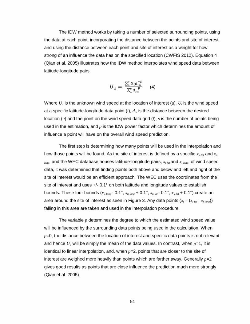
51

The IDW method works by taking a number of selected surrounding points, using

the data at each point, incorporating the distance between the points and site of interest,

and using the distance between each point and site of interest as a weight for how

strong of an influence the data has on the specified location (CWFIS 2012). Equation 4

(Qian et al. 2005) illustrates how the IDW method interpolates wind speed data between

latitude-longitude pairs.

∑

∑

(4)

Where Uu is the unknown wind speed at the location of interest (u), Ui is the wind speed

at a specific latitude-longitude data point (i), diu is the distance between the desired

location (u) and the point on the wind speed data grid (i), s is the number of points being

used in the estimation, and p is the IDW power factor which determines the amount of

influence a point will have on the overall wind speed prediction.

The first step is determining how many points will be used in the interpolation and

how those points will be found. As the site of interest is defined by a specific xu-lat and xu-

long, and the WEC database houses latitude-longitude pairs, xi-lat and xi-long, of wind speed

data, it was determined that finding points both above and below and left and right of the

site of interest would be an efficient approach. The WEC uses the coordinates from the

site of interest and uses +/- 0.1° on both latitude and longitude values to establish

bounds. These four bounds (xu-long - 0.1°, xu-long + 0.1°, xu-lat - 0.1°, xu-lat + 0.1°) create an

area around the site of interest as seen in Figure 3. Any data points (xi = (xi-lat , xi-long))

falling in this area are taken and used in the interpolation procedure.

The variable p determines the degree to which the estimated wind speed value

will be influenced by the surrounding data points being used in the calculation. When

p=0, the distance between the location of interest and specific data points is not relevant

and hence Uu will be simply the mean of the data values. In contrast, when p=1, it is

identical to linear interpolation, and, when p=2, points that are closer to the site of

interest are weighed more heavily than points which are farther away. Generally p=2

gives good results as points that are close influence the prediction much more strongly

(Qian et al. 2005).

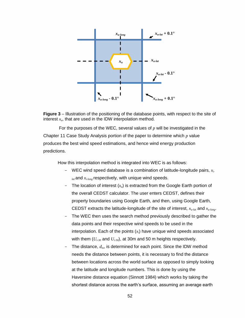
52

Figure 3 – Illustration of the positioning of the database points, with respect to the site of interest xu, that are used in the IDW interpolation method.

For the purposes of the WEC, several values of p will be investigated in the

Chapter 11 Case Study Analysis portion of the paper to determine which p value

produces the best wind speed estimations, and hence wind energy production

predictions.

How this interpolation method is integrated into WEC is as follows:

- WEC wind speed database is a combination of latitude-longitude pairs, xi-

lat and xi-long respectively, with unique wind speeds.

- The location of interest (xu) is extracted from the Google Earth portion of

the overall CEDST calculator. The user enters CEDST, defines their

property boundaries using Google Earth, and then, using Google Earth,

CEDST extracts the latitude-longitude of the site of interest, xu-lat and xu-long.

- The WEC then uses the search method previously described to gather the

data points and their respective wind speeds to be used in the

interpolation. Each of the points (xi) have unique wind speeds associated

with them (Ui-30 and Ui-50), at 30m and 50 m heights respectively.

- The distance, diu, is determined for each point. Since the IDW method

needs the distance between points, it is necessary to find the distance

between locations across the world surface as opposed to simply looking

at the latitude and longitude numbers. This is done by using the

Haversine distance equation (Sinnott 1984) which works by taking the

shortest distance across the earth’s surface, assuming an average earth

xu xu-lat

xu-lat + 0.1°

xu-lat - 0.1°

xu-long

xu-long - 0.1° xu-long + 0.1°

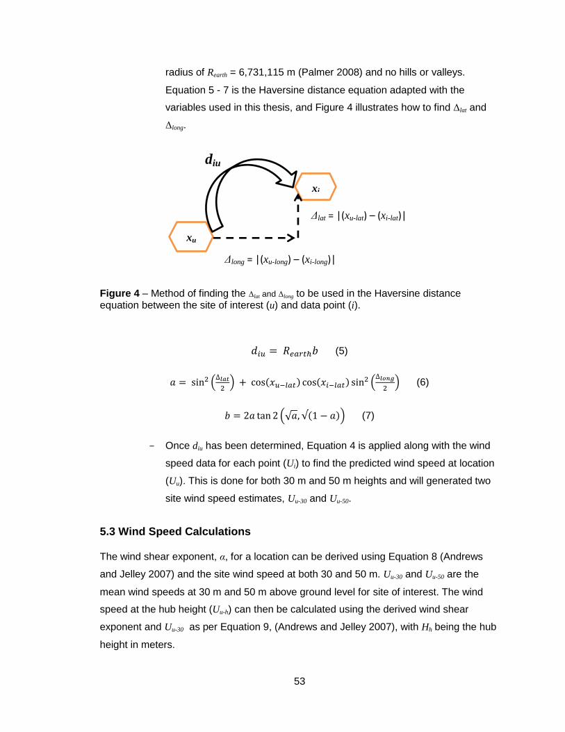
53

radius of Rearth = 6,731,115 m (Palmer 2008) and no hills or valleys.

Equation 5 - 7 is the Haversine distance equation adapted with the

variables used in this thesis, and Figure 4 illustrates how to find Δlat and

Δlong.

Figure 4 – Method of finding the Δlat and Δlong to be used in the Haversine distance equation between the site of interest (u) and data point (i).

(5)

(

)

(

) (6)

(√ √ ) (7)

- Once diu has been determined, Equation 4 is applied along with the wind

speed data for each point (Ui) to find the predicted wind speed at location

(Uu). This is done for both 30 m and 50 m heights and will generated two

site wind speed estimates, Uu-30 and Uu-50.

5.3 Wind Speed Calculations

The wind shear exponent, α, for a location can be derived using Equation 8 (Andrews

and Jelley 2007) and the site wind speed at both 30 and 50 m. Uu-30 and Uu-50 are the

mean wind speeds at 30 m and 50 m above ground level for site of interest. The wind

speed at the hub height (Uu-h) can then be calculated using the derived wind shear

exponent and Uu-30 as per Equation 9, (Andrews and Jelley 2007), with Hh being the hub

height in meters.

xu

xi

Δlong = |(xu-long) – (xi-long)|

Δlat = |(xu-lat) – (xi-lat)|

diu

54

(

)

(

)

(8)

(

)

(9)

Uu-h is now the average hub height wind speed for the site of interest and can

then be used in power production calculations.

5.4 Summary

This section has described the method through which the wind speed can be predicted

at the farmer’s property using the WEC program. It interpolates between grid points on a

5 km by 5 km world surface mesh of wind speed data generated by the CWEA and used

in the WEC database. There are no functions to increase the resolution of the wind

speed data, such as taking the effect of elevation, terrain, trees or building into account.

All of those factors, in addition to others, can have a significant impact on the wind

speed at a site (Andrews and Jelley 2007). While it is important to take them into

consideration, as explained in Chapter 9 – Wind Turbine Siting, incorporating them into

the wind speed prediction calculations adds many more variables and hence many

additional sources of potential error into the wind speed prediction.

55

Chapter 6 – Wind Turbine Properties

6.1 Turbine Size

With reliable wind speed data available for use in the WEC, it is now possible to assess

the wind energy potential at the site specified by the user. Although wind speed plays a

large role, power production is also influenced by the technical specifications of the wind

turbine. As a result, along with providing location information, the user of the WEC must

also select the turbine that best represents the project they are hoping to implement.

This chapter will address the turbine characteristics which influence power production,

which will be used when calculating the total power a turbine is expected to generate.

As mentioned at the beginning of this thesis, the Ontario Feed-in-Tariff program

has two divisions; MicroFIT (≤ 10 kW), and FIT (> 10 kW), and the tariff pricing has been

done according to technology type and project size (OPA 2010a). Based on Table 1, the

contract tariff price for wind turbines does not depend on turbine size, and hence there is

no apparent financial advantage to only looking at turbines with rated capacities of 10

kW or less. Instead the WEC will focus mainly on small scale wind turbines which are

rated between 0.3 kW - 300 kW (CanWEA 2010b). Although a turbine larger than 300

kW can generate more power, farmers generally will not have access to the capital funds

to install such a large turbine.

Turbines are normally sized based on their rated power. This is generally

representative of the maximum power a turbine can produce if it were to operate

continuously with optimal wind conditions (Andrews and Jelley 2007); hence a 10 kW

turbine can generate, at most, approximately 10 kW of power.

In many cases, farmers will not know the exact size of turbine they hope to

install. To aid in this decision, information provided by the Canadian Wind Energy

Association (CanWEA 2010c, 2010d) and summarized in Table 5, is included within the

WEC. This is to help farmers see a brief breakdown of size and use of a turbine, see

rough estimates of project costs, and direct them towards the size that would be most

desirable for their application.

56

Table 5 – Wind turbine size and application comparison (adapted from CanWEA 2010c, 2010d).

Turbine Size

Potential Applications Estimated Project

Cost

1.5 kW Residential - supplies approximately 300

kWh/month, approximately equivalent to 1/3 of an average household's electricity demands

$9,000

0.5-10 kW Residential Applications $3,000 - $60,000

10-50 kW Farm Applications $60,000 - $165,000

>20 kW Commercial and Small Industrial Applications >$120,000

6.2 Wind Turbine Models

With context provided as to turbine size, application, and cost relationships, a choice

must be made as to which specific turbine the user wants to consider, including:

manufacturer, rated power, and turbine height. Table 6 provides information on turbines

and towers produced by different manufacturers that are commonly installed in Ontario

and is incorporated into the WEC as a database. To simplify the WEC inputs required by

the user, the different turbine models listed are provided in a drop down list and

organized according to rated power. Once turbine manufacture and size are selected,

the corresponding rotor diameter and tower height(s) are then pulled from the database.

6.3 Rotor Diameter and Hub Height

Both rotor diameter and hub height, illustrated in Figure 5, influence the overall power

production of a turbine. Rotor diameter is equal to the diameter of the circle created by

the rotating blades and the hub height is the distance above the ground of the turbine

hub, which is the central point the blades rotate around. In many cases tower height and

hub height are approximately the same. Additionally, the swept area of a turbine is the

area of the circle the blades create.

57

Table 6 – Rotor diameter and potential tower heights for the small wind turbine models that will be incorporated into the WEC database.

Company Wind Turbine

Size (kW) Rotor

Diameter (m) Available Tower

Heights (m)

Aeronautica (AWP 2012)

225 29 30 - 50

Bergey Windpower (BWP 2012)

10 7 18 - 49

Endurance (EWP 2011)

5 - 50 6.37 - 19.2 27.5 - 36.6

Energie (Energie PGE 2012)

35 - 50 19.2 24 - 42

Eoltec (Eoltec 2010)

6 5.6 18 - 30

Northern Power Systems (NPS 2011)

100 21 30 - 37

ReDriven (ReD 2012)

5 - 50 3.9 - 9.2 12 - 36.6

Seaforth Energy (SE 2012a)

50 15 30 - 37

Southwest Windpower (SWWP 2011)

2.4 - 3 3.7 - 4.5 10.2 - 24

Ventera (VE 2010)

10 6.7 15 - 40

Vergnet (VWT 2012)

275 32 35.4

Wenvor Technologies Inc. (Wenvor 2009)

30 10 24 - 30

Wind Energy Solutions (WES 2012)

50 - 250 20 - 30 24 - 48

Figure 5 – Diagram illustrating wind turbine hub height and rotor diameter (Clarke 2003).

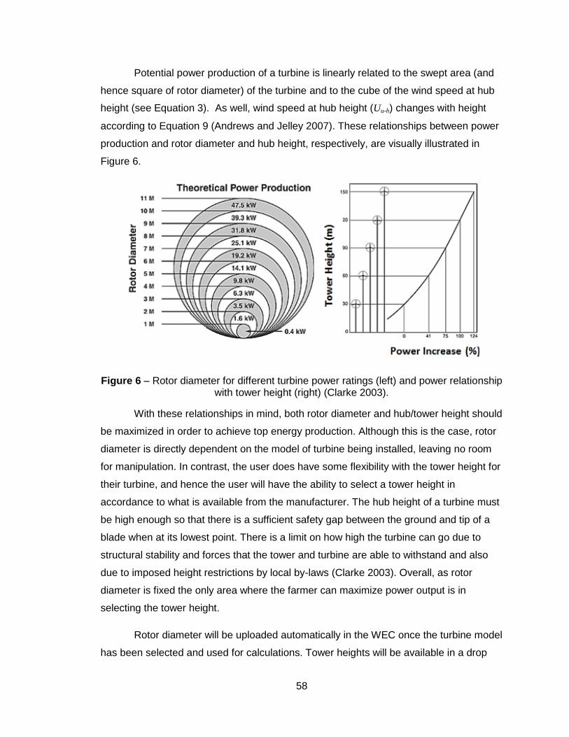
58

Potential power production of a turbine is linearly related to the swept area (and

hence square of rotor diameter) of the turbine and to the cube of the wind speed at hub

height (see Equation 3). As well, wind speed at hub height (Uu-h) changes with height

according to Equation 9 (Andrews and Jelley 2007). These relationships between power

production and rotor diameter and hub height, respectively, are visually illustrated in

Figure 6.

Figure 6 – Rotor diameter for different turbine power ratings (left) and power relationship with tower height (right) (Clarke 2003).

With these relationships in mind, both rotor diameter and hub/tower height should

be maximized in order to achieve top energy production. Although this is the case, rotor

diameter is directly dependent on the model of turbine being installed, leaving no room

for manipulation. In contrast, the user does have some flexibility with the tower height for

their turbine, and hence the user will have the ability to select a tower height in

accordance to what is available from the manufacturer. The hub height of a turbine must

be high enough so that there is a sufficient safety gap between the ground and tip of a

blade when at its lowest point. There is a limit on how high the turbine can go due to

structural stability and forces that the tower and turbine are able to withstand and also

due to imposed height restrictions by local by-laws (Clarke 2003). Overall, as rotor

diameter is fixed the only area where the farmer can maximize power output is in

selecting the tower height.

Rotor diameter will be uploaded automatically in the WEC once the turbine model

has been selected and used for calculations. Tower heights will be available in a drop

59

down menu that will change depending on turbine model selected and the user will have

the ability to choose the height they wish for their project.

6.4 Power Curve

The power curve of a wind turbine represents the amount of power produced at specific

wind speeds and plays a critical role in determining power production. Each turbine size

and model has a unique power performance curve. For example, Figure 7 illustrates the

specific power curve for a Bergey EXCEL 10kW wind turbine (BWP 2011) (the turbine

used in many case studies in the Chapter 11).

The cut-in wind speed for turbines is generally around 4 m/s (RI 2004b) for larger

turbines and is when the turbine starts to rotate and produce power. Slower winds do not

produce the necessary force to keep the turbine rotating and thus it is not economical to

allow them to run in this speed range. Although this is seen for most turbines, small

turbines, with low power ratings and light blades, might begin generating power even

before the wind speed reaches 4 m/s. This is seen with the Bergey EXCEL 10 in Figure

7 where the cut-in wind speed is 3 m/s (BWP 2011).

The power production reaches its rated power when winds reach the rated wind

speed, which is the speed the turbine is designed to operate at (Andrews and Jelley

2007). In the case of Figure 7 the rated power, 10 kW, is achieved at around 11.5 m/s.

Although wind speed continues to increase, the turbine is only designed for a certain

power rating and load. With faster winds the wind turbine blades rotate, or ‘change

pitch’, in order to reduce the load on the turbine, though this also limits the amount of

power that can be produced. At the point of the cut-out wind speed turbines stop

operating and power production drops to zero. This is done to prevent damage to the

turbine that can result from very strong winds. This is done to prevent damage to the

turbine that can result from very strong winds. It is seen for all sizes of turbines and

occurs normally around 25 m/s (RI 2004b).

The details regarding the performance and power curve of a turbine are generally

provided by the manufacturer. If the power coefficient (CP) is provided instead of the

power curve itself, CP can be used to generate the curve using Equation 3 (Andrews and

Jelley 2007).

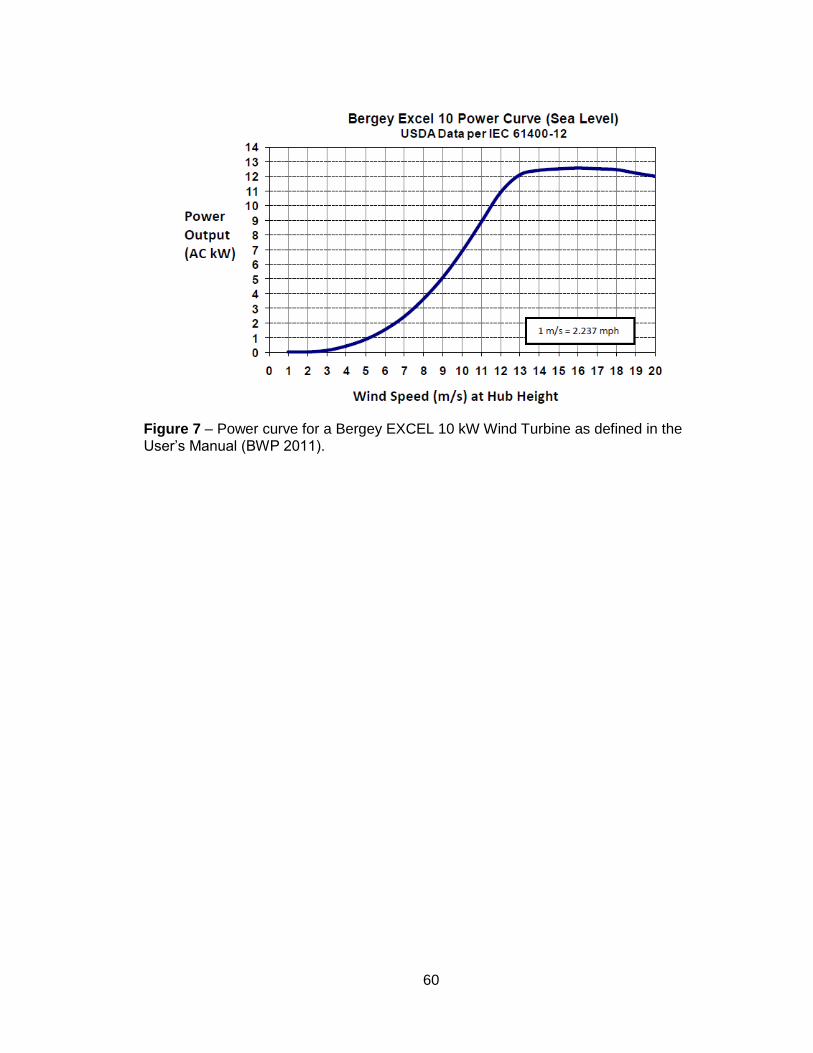
60

Figure 7 – Power curve for a Bergey EXCEL 10 kW Wind Turbine as defined in the User’s Manual (BWP 2011).

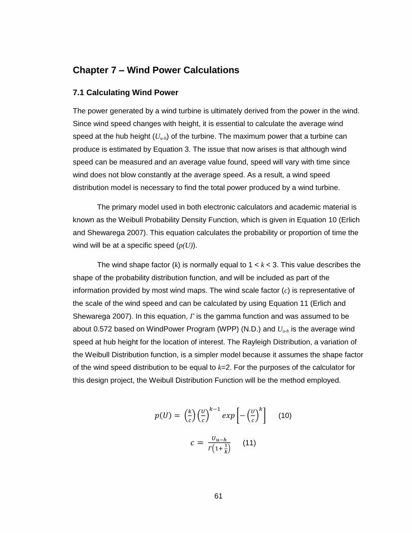
61

Chapter 7 – Wind Power Calculations

7.1 Calculating Wind Power

The power generated by a wind turbine is ultimately derived from the power in the wind.

Since wind speed changes with height, it is essential to calculate the average wind

speed at the hub height (Uu-h) of the turbine. The maximum power that a turbine can

produce is estimated by Equation 3. The issue that now arises is that although wind

speed can be measured and an average value found, speed will vary with time since

wind does not blow constantly at the average speed. As a result, a wind speed

distribution model is necessary to find the total power produced by a wind turbine.

The primary model used in both electronic calculators and academic material is

known as the Weibull Probability Density Function, which is given in Equation 10 (Erlich

and Shewarega 2007). This equation calculates the probability or proportion of time the

wind will be at a specific speed (p(U)).

The wind shape factor (k) is normally equal to 1 < k < 3. This value describes the

shape of the probability distribution function, and will be included as part of the

information provided by most wind maps. The wind scale factor (c) is representative of

the scale of the wind speed and can be calculated by using Equation 11 (Erlich and

Shewarega 2007). In this equation, is the gamma function and was assumed to be

about 0.572 based on WindPower Program (WPP) (N.D.) and Uu-h is the average wind

speed at hub height for the location of interest. The Rayleigh Distribution, a variation of

the Weibull Distribution function, is a simpler model because it assumes the shape factor

of the wind speed distribution to be equal to k=2. For the purposes of the calculator for

this design project, the Weibull Distribution Function will be the method employed.

(

) (

)

[ (

)

] (10)

(

) (11)

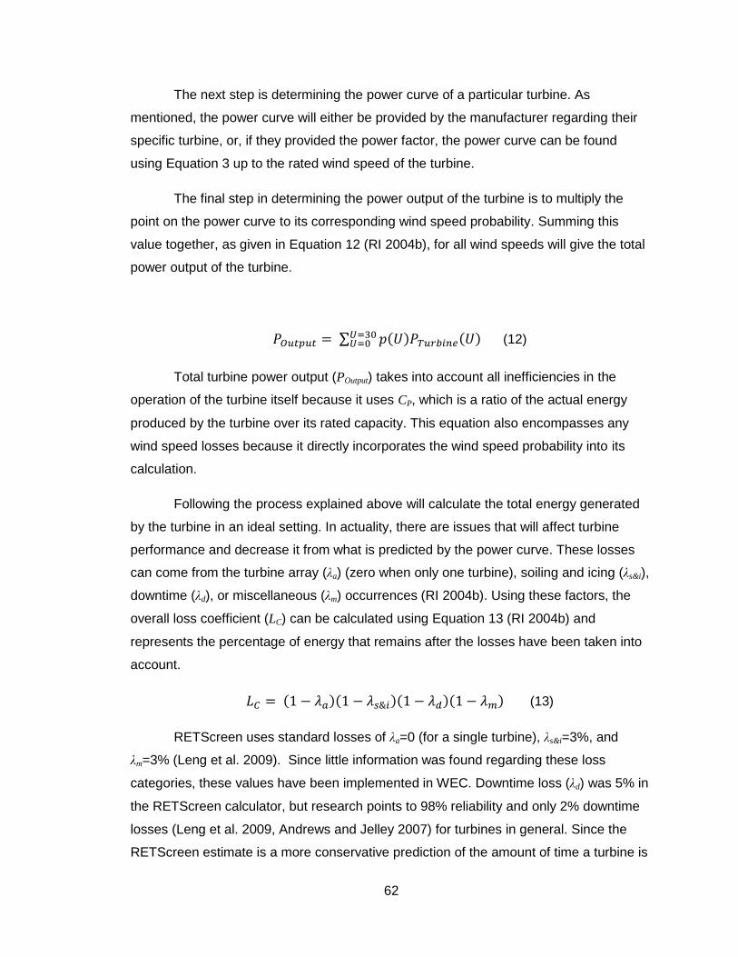
62

The next step is determining the power curve of a particular turbine. As

mentioned, the power curve will either be provided by the manufacturer regarding their

specific turbine, or, if they provided the power factor, the power curve can be found

using Equation 3 up to the rated wind speed of the turbine.

The final step in determining the power output of the turbine is to multiply the

point on the power curve to its corresponding wind speed probability. Summing this

value together, as given in Equation 12 (RI 2004b), for all wind speeds will give the total

power output of the turbine.

∑ (12)

Total turbine power output (POutput) takes into account all inefficiencies in the

operation of the turbine itself because it uses CP, which is a ratio of the actual energy

produced by the turbine over its rated capacity. This equation also encompasses any

wind speed losses because it directly incorporates the wind speed probability into its

calculation.

Following the process explained above will calculate the total energy generated

by the turbine in an ideal setting. In actuality, there are issues that will affect turbine

performance and decrease it from what is predicted by the power curve. These losses

can come from the turbine array (λa) (zero when only one turbine), soiling and icing (λs&i),

downtime (λd), or miscellaneous (λm) occurrences (RI 2004b). Using these factors, the

overall loss coefficient (LC) can be calculated using Equation 13 (RI 2004b) and

represents the percentage of energy that remains after the losses have been taken into

account.

(13)

RETScreen uses standard losses of λa=0 (for a single turbine), λs&i=3%, and

λm=3% (Leng et al. 2009). Since little information was found regarding these loss

categories, these values have been implemented in WEC. Downtime loss (λd) was 5% in

the RETScreen calculator, but research points to 98% reliability and only 2% downtime

losses (Leng et al. 2009, Andrews and Jelley 2007) for turbines in general. Since the

RETScreen estimate is a more conservative prediction of the amount of time a turbine is

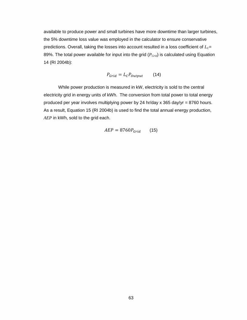
63

available to produce power and small turbines have more downtime than larger turbines,

the 5% downtime loss value was employed in the calculator to ensure conservative

predictions. Overall, taking the losses into account resulted in a loss coefficient of LC=

89%. The total power available for input into the grid (PGrid) is calculated using Equation

14 (RI 2004b):

(14)

While power production is measured in kW, electricity is sold to the central

electricity grid in energy units of kWh. The conversion from total power to total energy

produced per year involves multiplying power by 24 hr/day x 365 day/yr = 8760 hours.

As a result, Equation 15 (RI 2004b) is used to find the total annual energy production,

AEP in kWh, sold to the grid each.

(15)

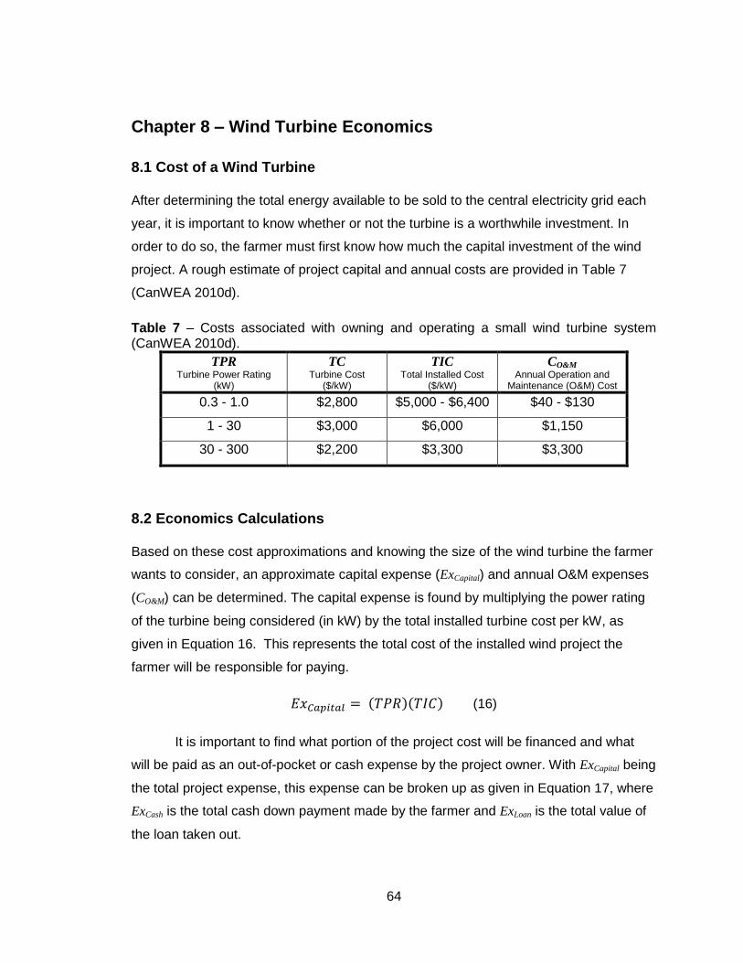
64

Chapter 8 – Wind Turbine Economics

8.1 Cost of a Wind Turbine

After determining the total energy available to be sold to the central electricity grid each

year, it is important to know whether or not the turbine is a worthwhile investment. In

order to do so, the farmer must first know how much the capital investment of the wind

project. A rough estimate of project capital and annual costs are provided in Table 7

(CanWEA 2010d).

Table 7 – Costs associated with owning and operating a small wind turbine system (CanWEA 2010d).

TPR Turbine Power Rating

(kW)

TC Turbine Cost

($/kW)

TIC Total Installed Cost

($/kW)

CO&M

Annual Operation and Maintenance (O&M) Cost

0.3 - 1.0 $2,800 $5,000 - $6,400 $40 - $130

1 - 30 $3,000 $6,000 $1,150

30 - 300 $2,200 $3,300 $3,300

8.2 Economics Calculations

Based on these cost approximations and knowing the size of the wind turbine the farmer

wants to consider, an approximate capital expense (ExCapital) and annual O&M expenses

(CO&M) can be determined. The capital expense is found by multiplying the power rating

of the turbine being considered (in kW) by the total installed turbine cost per kW, as

given in Equation 16. This represents the total cost of the installed wind project the

farmer will be responsible for paying.

(16)

It is important to find what portion of the project cost will be financed and what

will be paid as an out-of-pocket or cash expense by the project owner. With ExCapital being

the total project expense, this expense can be broken up as given in Equation 17, where

ExCash is the total cash down payment made by the farmer and ExLoan is the total value of

the loan taken out.

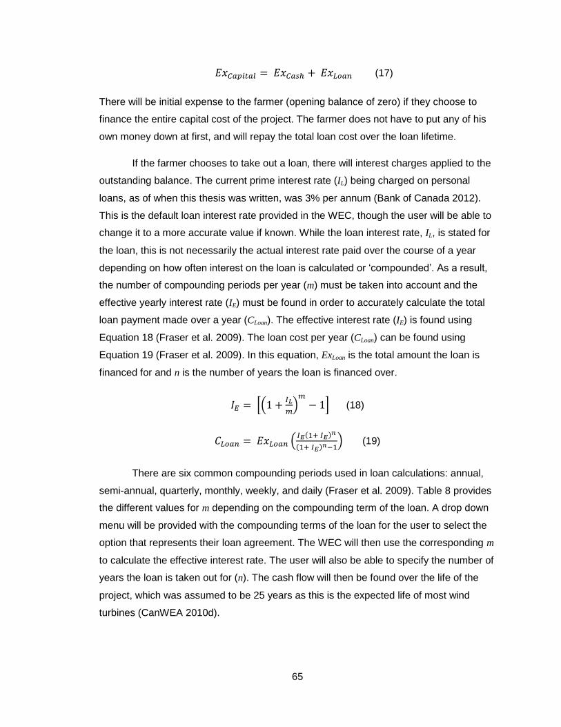
65

(17)

There will be initial expense to the farmer (opening balance of zero) if they choose to

finance the entire capital cost of the project. The farmer does not have to put any of his

own money down at first, and will repay the total loan cost over the loan lifetime.

If the farmer chooses to take out a loan, there will interest charges applied to the

outstanding balance. The current prime interest rate (IL) being charged on personal

loans, as of when this thesis was written, was 3% per annum (Bank of Canada 2012).

This is the default loan interest rate provided in the WEC, though the user will be able to

change it to a more accurate value if known. While the loan interest rate, IL, is stated for

the loan, this is not necessarily the actual interest rate paid over the course of a year

depending on how often interest on the loan is calculated or ‘compounded’. As a result,

the number of compounding periods per year (m) must be taken into account and the

effective yearly interest rate (IE) must be found in order to accurately calculate the total

loan payment made over a year (CLoan). The effective interest rate (IE) is found using

Equation 18 (Fraser et al. 2009). The loan cost per year (CLoan) can be found using

Equation 19 (Fraser et al. 2009). In this equation, ExLoan is the total amount the loan is

financed for and n is the number of years the loan is financed over.

[(

)

] (18)

(

) (19)

There are six common compounding periods used in loan calculations: annual,

semi-annual, quarterly, monthly, weekly, and daily (Fraser et al. 2009). Table 8 provides

the different values for m depending on the compounding term of the loan. A drop down

menu will be provided with the compounding terms of the loan for the user to select the

option that represents their loan agreement. The WEC will then use the corresponding m

to calculate the effective interest rate. The user will also be able to specify the number of

years the loan is taken out for (n). The cash flow will then be found over the life of the

project, which was assumed to be 25 years as this is the expected life of most wind

turbines (CanWEA 2010d).

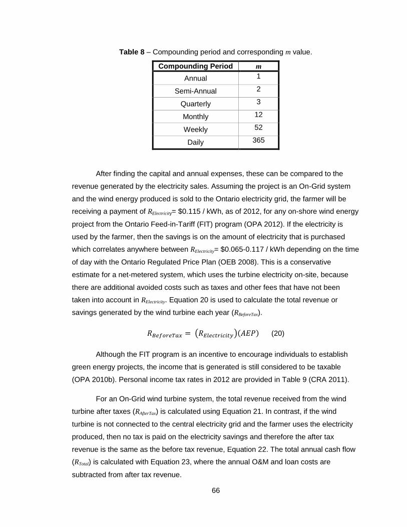
66

Table 8 – Compounding period and corresponding m value.

Compounding Period m

Annual 1

Semi-Annual 2

Quarterly 3

Monthly 12

Weekly 52

Daily 365

After finding the capital and annual expenses, these can be compared to the

revenue generated by the electricity sales. Assuming the project is an On-Grid system

and the wind energy produced is sold to the Ontario electricity grid, the farmer will be

receiving a payment of RElectricity= $0.115 / kWh, as of 2012, for any on-shore wind energy

project from the Ontario Feed-in-Tariff (FIT) program (OPA 2012). If the electricity is

used by the farmer, then the savings is on the amount of electricity that is purchased

which correlates anywhere between RElectricity= $0.065-0.117 / kWh depending on the time

of day with the Ontario Regulated Price Plan (OEB 2008). This is a conservative

estimate for a net-metered system, which uses the turbine electricity on-site, because

there are additional avoided costs such as taxes and other fees that have not been

taken into account in RElectricity. Equation 20 is used to calculate the total revenue or

savings generated by the wind turbine each year (RBeforeTax).

( ) (20)

Although the FIT program is an incentive to encourage individuals to establish

green energy projects, the income that is generated is still considered to be taxable

(OPA 2010b). Personal income tax rates in 2012 are provided in Table 9 (CRA 2011).

For an On-Grid wind turbine system, the total revenue received from the wind

turbine after taxes (RAfterTax) is calculated using Equation 21. In contrast, if the wind

turbine is not connected to the central electricity grid and the farmer uses the electricity

produced, then no tax is paid on the electricity savings and therefore the after tax

revenue is the same as the before tax revenue, Equation 22. The total annual cash flow

(RTotal) is calculated with Equation 23, where the annual O&M and loan costs are

subtracted from after tax revenue.

67

Table 9 – Canadian federal and Ontario provincial personal income tax rates (CRA

2011).

Federal – Canadian Provincial – Ontario

Range of Income Tax Rate (IF) Income Range Tax Rate (IP)

$0 – $42,707 15% $0 – $39,020 5.05%

$42,707 – $85,414 22% $39,021 – $78,034 9.15%

$85,414 – $132,406 26% > $78,034 11.16%

>$132,406 29%

( )( ) On Grid System (21)

Net Metered System (22)

(23)

The Cumulative Cash Flow (CCn) throughout the project can be calculated by

adding the RTotal to initial expenses incurred by the farmer (ExCash) for the first year. This

amount represents the net cash flow of the project each year and can be found using

Equation 24:

(24)

In instances where the entire project cost was financed, the CC0 will be equal to

zero. In this case, if the RTotal>0 then the farmer can make money off of the project over

the analysis period and it can represent an economically viable project. If RTotal<0 the

farmer experiences a loss every year and thus the project is not financially feasible.

In other cases where the farmer had a cash down payment on the project initially,

this payment represents a negative, non-zero ExCash cash flow and RTotal will be added to

this number on a yearly basis. Assuming that the RTotal is positive (representing a yearly

gain), there may come a point where the revenue generated over a number of years has

caused the CCn≥0. This means that the farmer has gained back the money he initially

put into the project, and the year ‘n’ where CCn=0 is known as the Payback Period. The

feasibility of the project is a very subjective assessment as some individuals will view a

68

project as financially viable where others will not. In general, a good indicator of

feasibility for renewable energy projects is if the payback period of the project less than

about 10-15 years.

The final step in examining the economics of the wind turbine feasibility would be

to present the user with a value for a return on investment (ROI). In this case, the return

on investment provides a number corresponding to the percentage return the investor

sees on their original investment. Specifically the ROI would show the farmer the

percentage of the total project cost (ExCapital) either gained (positive) or lost (negative) at

the end of the turbine’s lifetime (CC25), Equation 25.

(

) (25)

69

Chapter 9 – Wind Turbine Siting

9.1 Importance of Turbine Siting

At this point, many of the basics of wind energy have been addressed including: the

decision making process, resource availability, turbine properties, and how the energy

and economic calculations are performed. While all of this information is essential for

producing a reliable wind energy assessment, if the results and findings of the

assessment are not implemented properly then it will not matter how reliable the

assessment was.

One of the most critical aspects of a site specific wind energy feasibility study is

turbine siting. Siting of a turbine involves determining the precise placement of the

turbine on a piece of property. Even if turbine predictions are fully accurate, if the wind

turbine is placed incorrectly on the property then the prediction has no value. For

example, if turbines are placed too close to buildings the wind flow is disturbed and the

wind speed, and therefore energy production, could be significantly lower than WEC

predictions. To assist with proper siting, placement guidelines are explained below and

will be incorporated into the WEC program.

9.2 Ontario Turbine Classifications and Guidelines

There are different regulations that must be met for the turbine to be installed at a

specific site depending on the location and size of a turbine. As the CEDST program is

intended for Ontario applications, regulations set forth by the Government of Ontario are

those applicable to this project. The Ontario Government created the Environmental

Protection Act (Ontario Regulation 359/09) within which Renewable Energy Approvals

are provided in Part V.0.1 (GoO 2011a). Ontario has set out five classes of wind turbines

and developed siting regulations for each turbine class (Table 10).

Class 1 and 2 wind turbines are small in size to larger turbines and do not have

any regulations regarding minimum setback distances from property lines, roads, rail

lines, or buildings, whereas Class 3, 4, and 5 turbines have strict regulations (GoO

2011a). A ‘Noise Receptor’ is defined as the location at which noise generated from a

renewable energy system is received (GoO 2011b), most often a noise receptor is a

building in which people live, work, or occupy. Table 11 provides the minimum provincial

70

setbacks for the Class 3, 4 and 5 turbines for the setbacks. Here, the setback is defined

as the distance from the centre of the turbine base to the location of interest (GoO

2011a).

Table 10 – Definition of wind turbine classes within the Ontario government regulations (GoO 2011b).

Wind Turbine Class

Size Noise Contact with surface water

Class 1 ≤ 3 kW Any No

Class 2 > 3 kW and < 50 kW Any No

Class 3 ≥ 50 kW < 102 dBA No

Class 4 ≥ 50 kW ≥ 102 dBA No

Class 5 Any Any Yes

Table 11 – Setback regulations for Class 3, 4 and 5 wind turbines in Ontario (GoO 2011a).

Point of Interest Minimum Setback

Property Line height of turbine (excluding blade length)

Road blade length + 10 m

Railway Line blade length + 10 m

Noise Receptors ≥ 550 m (specific turbine noise to setback matrix)

Turbines rated at 50 kW and greater must adhere to specific setback regulations.

From these regulations, the most stringent being the 550 m setback from noise

receptors, issues could arise where the property size and noise receptor location could

restrict the size of turbine allowed to be installed by a farmer. For example, a small farm

may have their or a neighbour’s house within the 550 m setback radius and therefore the

farmer is limited to installing a wind turbine rated at less than 50 kW.

With this setback condition, and also the estimated cost of a 50kW turbine being

approximately $165,000 (Table 5), it is anticipated that most farmers using the CEDST

WEC will be looking to install a turbine smaller than 50 kW. Though if a farmer does wish

to install a 50 kW turbine or larger, they must then ensure that the aforementioned

setback regulations are met when siting the turbine.

71

9.3 Small Wind Turbine Guidelines

As mentioned, turbines less than 50 kW do not have any setback regulations associated

with them in Ontario, though there are still recommended placement guidelines to

maximize energy production and minimize wear and tear on the turbine. These

recommendations are outlined for the 3-50 kW small wind turbines (GoO 2011c).

Additionally, this section reveals that while there are no provincial requirements for small

turbine siting, there may be municipal requirements that must be met which are specific

to the municipality the property is part of, and hence the farmer must investigate these

on a case by case basis.

9.3.1 Property Lines

There are a number of proximity guidelines established, but it is strongly advised that the

individual wishing to install a turbine first start by notifying and discussing the idea with

neighbours before construction begins. It is suggested that small turbines be placed at

least six to nine metres from any property line (Rhoads-Weaver et al. 2006), though this

can vary anywhere between zero times to four times the turbine tower height depending

upon municipality by-laws (Rhoads-Weaver et al. 2006). For example, in 2005 the

property line setback requirement in Malahide, Ontario was set to be 1.2 times the tower

height of a turbine and, in Simcoe County, the regulation was defined as 1.5 times the

tower height (Rhoads-Weaver et al. 2006).

9.3.2 Buildings, Man-made Structures, and Vegetation – Setbacks

The minimum setback recommendation for buildings, man-made structures (such as

power lines), and vegetation is one tower height (Rhoads-Weaver et al. 2006). This

recommendation comes about as it gives sufficient working area around the base of the

turbine for construction and maintenance activities to occur.

One tower height this is the minimum recommendation, though there are other

factors that must be taken into account. Buildings, vegetation, and other features act as

obstacles to wind. Wind gets forced up and over these obstacles which severely

changes wind velocity and increases turbulence. If these wind impedances are

downwind of a wind turbine, they are less likely to influence turbine performance.

Conversely, upwind obstacles impact wind flow through a turbine and can drastically

impact turbine performance. Slower wind speeds translate to less energy production.

72

Additionally, the increased turbulence amplifies vibration and changes the forces

working on the turbine accelerating wear and tear (Rhoads-Weaver et al. 2008). The

effect of the obstacle on the wind decreases with increasing distance from the obstacle

and therefore eventually the wind’s speed and laminar flow will return.

With this in mind, it is not advisable to put a turbine close to wind obstacles, both

up and downstream, as wind direction constantly changes and the turbine rotates about

the tower in order to face the wind. Of the research performed, the smallest

recommended offset between obstacle and turbine was ten times the height of the

obstacle (RU 2010), but a more common recommendation was 20 times (NWCE [N.D.]b,

Rhoads-Weaver et al. 2008) with a minimum of 100 m separation with obstacles of

approximately the same height (Rhoads-Weaver et al. 2008). Using the guideline of

twenty times the obstacle height between the obstacle and the turbine, coupled with

turbine height recommendations, ensures that the wind has regained much of its original

speed and flow pattern. This is recommendation is illustrated in Figure 8.

Figure 8 – Wind turbine separation recommendations (DoE 2007).

9.3.3 Buildings, Man-made Structures, and Vegetation – Height Recommendations

In addition to a setback between obstacles and turbines, there are height guidelines as

well. Turbulence extends to a level twice the height of the obstacle in the downstream

flow, as illustrated in Figure 8 (Rhoads-Weaver et al. 2008, GoE 2007). As a result, it is

73

recommended that there be a height difference between the top of the highest obstacle

in the turbine proximity and the bottom tip of the blades of either three times the blade

length, or eight to nine metres, whichever is greater (Rhoads-Weaver et al. 2006;

Rhoads-Weaver et al. 2008). With these guidelines, the minimum height of the turbine

can be determined.

9.3.4 Roof Top Turbines

There are instances where small turbines are designed to be attached to the roof of

buildings. While this may be how the turbines are designed and the owner would see

some performance out of the turbine, this may not be the optimal site for many turbines

(Lubitz and Hakimi 2008). The Guelph Case Study in Chapter 11 supports this position.

9.4 Relating Setback and Height to the WEC

Using these recommendations it is possible for the WEC to aid in helping the user

identify what areas of the property represent acceptable areas for turbine placement and

turbine height suggestions. Utilizing either user inputted building and vegetation heights,

or standard height values if exact heights are not known to the user, the WEC is able to

compute the minimum recommended tower height for the turbine. Additionally, these

heights can be used to find obstacle-turbine separation.

With a Google Earth interface incorporated into CEDST, the user will be able to

outline their property line and identify buildings and treelines on the property. With this

feature, as well as knowing obstacle height and setback recommendations, the CEDST

WEC will be able to create an overlay of the property which highlights the area

acceptable for turbine placement.

9.5 What Makes an Ideal Wind Site?

Many of the specific parameters for turbine siting have been presented. While it is

important to take these recommendations into account when determining the final

location of the turbine, intuition and also visual examination of the property can be

incredibly valuable.

Of course, the most promising way to choose a wind turbine site is to directly

measure the wind speeds at multiple locations and select the one with the highest wind

74

speed, but, as explained in Chapter 4.1, this is an expensive and time consuming

process that starts at a minimum of $10,000 and one year of data collection (RI 2004a,

NWCE [N.D.]a).

For a site to potentially be economically viable for a wind turbine project, the

minimum yearly average wind speed should be at least 4 m/s at ten metres above

ground level (Clarke 2003, RI 2004b). Wind speed is the most important factor when

siting a wind turbine, but there are also other constraints.

For individuals hoping to connect their turbine to the grid and FIT program, they

must first determine whether the closest grid connection is within a reasonable distance,

and then must determine whether there is available capacity in that grid line to handle

the electricity that would be produced by the turbine (NWCE [N.D.]c). If the connection

point is far away, costs to connect to the grid may be extremely high and make the

project unfeasible. As well, if there is no available capacity then the turbine will not be

able to be part of the FIT program.

Features that make building turbines more difficult include steep slopes and soil

or substrate condition (NWCE [N.D.]b). Steeps slopes make construction much harder

and thus can come with increased project costs. Additionally, if the soil or substrate is

too hard and requires blasting in order to properly secure the turbine, this again makes

the project more costly (NWCE [N.D.]b). Increasing project costs minimizes the overall

project return and therefore can cause the project to be assessed as uneconomical.

Similar to obstacles, ridgelines and hilltops can result in turbulence in wind flow

as they abruptly change flow direction. Knowing this, the turbines should be setback

from the edges of ridges and hills to minimize the turbulence the turbine experiences

(NWCE [N.D.]b).

Ideally, there are a few types of terrain that best suit wind turbines. Flat planes

with low wind shear exponents allow the wind to flow uninhibited and hence gain speed

while maintaining a laminar flow pattern. This lowers the loads and stresses seen on the

turbine (RI 2004b), reducing wear on the turbine and making the rotor easier to turn.

Additionally, hills and valleys can increase wind speed, as the wind must speed up due

to compressed streamlines and, if the elevation change is sufficiently gradual, there will

75

not be a flow disruption and the flow will remain laminar. As a result, the flow will be fast

and stable and therefore optimal for siting a turbine.

9.6 Concerns Over Turbine Location

Many of the anti-wind turbine activists who work at protesting and preventing wind

turbine development, of both small and large turbines, raise concerns about wind turbine

locations. Their concerns include health and hearing issues, in addition to a perceived

decrease in property value as a result of neighbouring turbines.

The setbacks from noise receptors prevent any hearing damage from occurring

(CMOH 2010). In terms of health, there are no studies currently available that confirm

that turbines cause health issues when they follow reasonable setbacks (CMOH 2010),

but there are studies continually monitoring this concern. Additionally, while there is

insufficient data in Canada, studies in the United States have found that there are no

statistically significant impacts from wind turbines on nearby property value (Rhoads-

Weaver et al. 2006). In some cases it has been observed that property value rises faster

in those areas when compared to others (Rhoads-Weaver et al. 2006).

Overall, installing a turbine in accordance to the regulations, recommendations,

and visual observation helps ensure that the turbine will perform at optimal conditions

and not cause any harm to individuals. The WEC is able to help with this by highlighting

acceptable turbine locations on the user’s property.

76

Chapter 10 – Wind Turbine: Case Study Availability

10.1 Case Study Search

In order to validate the CEDST WEC, the predictions produced by the WEC needed to

be evaluated in case studies. The goals of the case studies were to show that the WEC

is comparable or better than other wind resource prediction tools available and to

determine how well WEC predictions correlate to actual energy production by real

turbines.

The CEDST is specifically intended for renewable energy resource assessment

in Ontario and thus case studies would ideally involve Ontario wind turbines. Though

that would be ideal, finding small wind turbines in Ontario where the owners recorded

sufficient data for an evaluation and were willing to share their turbine’s energy

production data was difficult. In order for a site to be used as a case study both technical

specifications and recorded energy production for the turbine must be available.

10.1.1 Ontario

There are several small wind turbines in the immediate vicinity of Guelph, Ontario.

However, only one turbine was suitable as a case study. Those that were not suitable

were either non-operational or data available was insufficient for WEC validation.

One turbine in the Guelph area was used as a case study. A Wind Simplicity

Wind Dancer 7a (6.6 kW rated power), which had a 2.98 m rotor diameter, was installed

on 4 m, single, free-standing pole tower on the roof of the Guelph Emergency Services

Facility and was commissioned in April 2011 (Balean 2012). Power production data from

the turbine was able to be obtained for each month of production by reading the data off

of the inverter.

Expanding the search perimeter, turbines at commercial developments were

investigated. GO Transit/Metrolinx has a 50 kW FreeBreeze wind turbine at their Lisgar

GO Station (GO Transit 2011). After speaking with the Media Relations and Issues

Specialist on January 30, 2012, it was determined that this turbine could not be used as

part of this report. Similarly, the Hudson’s Bay Company (HBC) has installed wind

turbine on numerous Zellers and The Bay stores across the GTA region (HBC 2008,

77

McGuinness 2007). At The Bay – Conestoga Mall in Waterloo, there are two 1.8 kW

turbines (HBC 2008). Based on a phone conversation with the HBC Environmental

Manager for Enterprise Operations on March 9, 2012, it was determine that the small

amount of power the turbines produce is used in house and that HBC was not able to

share any information for use as a case study. The most recent commercial application

of wind turbines is at a Wal-Mart in Milton, Ontario (CNW 2011). The 20 kW turbine was

installed in 2011 but, at the time of this thesis, was still not fully commissioned and

recording power, according to Wal-Mart Canada’s Manager of Energy Efficiency

Programs (phone call 2012 Jan 11). As a result, even though Wal-Mart was willing to

work together with the CEDST project, any production data would not span a significant

enough timeframe for this project in order to perform a robust and illustrative case study.

Looking outside of commercial ownership, two owners of Bergey wind turbines

were found that are using the turbines to support their off-grid Ontario houses. One

home is located in Tamworth, Ontario and the other in Almonte, Ontario, having a 1.5kW

and 1.0kW Bergey wind turbine respectively (Mather 2012). Both of these families have

multiple different renewable systems to supply electricity to their off grid homes, and the

most substantial contribution comes from Solar PV systems (Mather 2012). As a result,

neither family had invested time into monitoring the production of their turbines and thus

they could not be used as case studies.

Overall, based on the response from Ontario wind turbine owners there are very

few owners that actually track their wind energy production and, those that do, are not

willing to disclose the information. As a result, there is a significant hole in the Ontario

wind energy community of available small wind turbine production and performance

data. This gap hinders wind turbine research and makes it difficult to determine how well

wind turbines are performing in comparison to predictions from wind energy calculators.

Therefore, the geographic scope had to be expanded in order to gather case study sites.

10.1.2 Nova Scotia

An egg farmer of Bayview Poultry Farms, in Nova Scotia graciously provided information

regarding the energy production for three small wind turbines installed on site. Bayview

Poultry Farms is located near Masstown, Nova Scotia (Figure 9) and has 3 Southwest

Windpower Skystream 3.7 wind turbines, with 2.4kW rated power capacity each (SE

2012b).

78

Figure 9 – Location of Bayview Poultry Farms.

While the turbines are not located in Ontario, the Canadian Wind Energy Atlas

(CWEA) has the same resolution of data across the entire country and thus it is still

possible to use this data in the WEC to perform wind energy production predictions. The

predictions can then be compared to the actual production to determine the accuracy of

the WEC. While these turbines are not located in Ontario, since the data is taken from

the same source and uses the same calculation methodology, the Nova Scotia case

studies are still able to reflect upon the WEC performance.

10.1.3 New York

Collaboration with Dr. Mel Tyree resulted in obtaining wind energy production data for

over twenty Excel 10 kW Bergey wind turbines in New York State, seventeen of which

had sufficient data for analysis. Figure 10 illustrates the approximate locations of each

of the available turbine sites in New York. Turbines were numbered 1 – 17 as labeled on

the map.

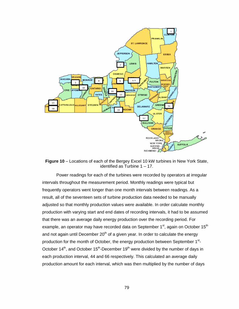
79

Figure 10 – Locations of each of the Bergey Excel 10 kW turbines in New York State, identified as Turbine 1 – 17.

Power readings for each of the turbines were recorded by operators at irregular

intervals throughout the measurement period. Monthly readings were typical but

frequently operators went longer than one month intervals between readings. As a

result, all of the seventeen sets of turbine production data needed to be manually

adjusted so that monthly production values were available. In order calculate monthly

production with varying start and end dates of recording intervals, it had to be assumed

that there was an average daily energy production over the recording period. For

example, an operator may have recorded data on September 1st, again on October 15th

and not again until December 20th of a given year. In order to calculate the energy

production for the month of October, the energy production between September 1st-

October 14th, and October 15th-December 19th were divided by the number of days in

each production interval, 44 and 66 respectively. This calculated an average daily

production amount for each interval, which was then multiplied by the number of days

80

that were in October, 14 for the first collection period and 17 for the second. Summing

these two values together produced the monthly production value for October.

Similar to the Nova Scotia case study, the turbines in New York did not present

ideally located case studies. Although that is the case, they can also still be used to

evaluate the WEC. The CWEA actually spans New York State (CWEA 2003a), in

addition to Canada, and therefore can be used to keep wind speed data source,

methodology, and resolution consistent to what is used for sites in Ontario.

81

Chapter 11 – Wind Turbine: Case Study Analysis

11.1 Case Study Intentions

As explained in the previous section there are multiple case study locations being used

in this thesis. There were a total of 19 locations able to produce valid case studies: one

in Guelph, Ontario, one near Masstown, Nova Scotia, and 17 in New York State.

In addition to actual energy production data, there were three different

predictions performed for the case studies. First, RETScreen was evaluated based on

what an individual with limited knowledge of wind energy systems and the program itself

would be able to produce. In this situation, it was assumed that the wind resource data

would be selected based off of the closest available city in RETScreen. This trial is used

to illustrate the scale of predictions that can be expected to be produced by a farmer

wishing to investigate wind energy and has some basic knowledge and familiarity with

wind energy technology and RETScreen. For labelling purposes, this scenario will be

referred to as ‘RETScreen (default)’.

Second, RETScreen was again utilized to generate energy production

predictions but used the wind speeds generated from the WEC methodology of the

CWEA database and also losses were identical to those used in the WEC. This trial was

performed to illustrate the difference in prediction between RETScreen and WEC using

identical input wind speed data. As this scenario involved manually inputting location

specific wind data generated from the database, it will be labelled as ‘RETScreen

(manual)’.

Third, the WEC was used in its full capacity to evaluate turbine sites. Results are

independent of the level of knowledge or familiarity of the user with operating the

program since the WEC is designed to be easy to both use and input accurate

information no matter the proficiency of the user with the WEC or in the wind industry.

11.2 Inverse Distance Weighted (IDW) Power Factor

In Section 5.2 of this thesis, it was explained that p is the power factor in Equation 6 that

determines the degree of influence that sites have when they are farther away from the

point of interest. Influence can be interpreted with the following reference points; p=0

82

meaning distance has no influence on the wind speed calculation, p=1 revealing that

wind speed is linearly related to the distance between points, and p=2 meaning that sites

closer to the location of interest exert more influence over the predicted wind speed than

sites farther away.

As part of the Case Study Analysis section and in order to produce the most

realistic WEC possible, an evaluation of different p values was performed. To do this,

three different wind speed predictions were performed for each site using p =1, 1.5, 2

respectively in the IDW calculations. Each of set of interpolated, predicted wind speeds

was entered into both RETScreen and the WEC in order to predict energy production by

the wind turbine.

Wind speed predictions for Guelph, Ontario, as shown in Figure 11, used the

different p values and are illustrative of cases where p has no influence on energy

production predictions as there is only a very small magnitude of difference between the

results values. Analysis for the Guelph turbine was performed at two heights, at tower

height and total above ground height, as it was a roof mounted turbine and it was hard to

determine what an appropriate turbine hub height would be. Of the nineteen case study

locations, four studies showed that there was no benefit of using one p value over

another.

The majority of locations demonstrated that while p has some influence on wind

energy production predictions, the difference is not significant, most within +/- 5% of

each other, as detailed in Table 12. The exclusions to this are the Nova Scotia turbines

which will be explained in the following paragraph. Two examples are provided in Figure

12 and Figure 13 for Turbine 7 and Turbine 11 respectively, selected based on their

clear representation of results. Turbine 7 demonstrated a case where p=2 gives slightly

more accurate results and Turbine 11 showed a slight benefit of using p=1 (though in

both cases there is only a small difference between the predicted values no matter the p

value used). Overall, of the fourteen remaining locations, the cases were split between

which p value showed better results, eight with p=1 being slightly better and the

remainder with p=2 generating slightly more favourable results.

The only location where a significant difference existed between the energy

predictions as a result of different IDW p values was in Nova Scotia, Figure 14, likely due

to Bayview Poultry Farms’ location. Geographically, the Nova Scotia turbines were the

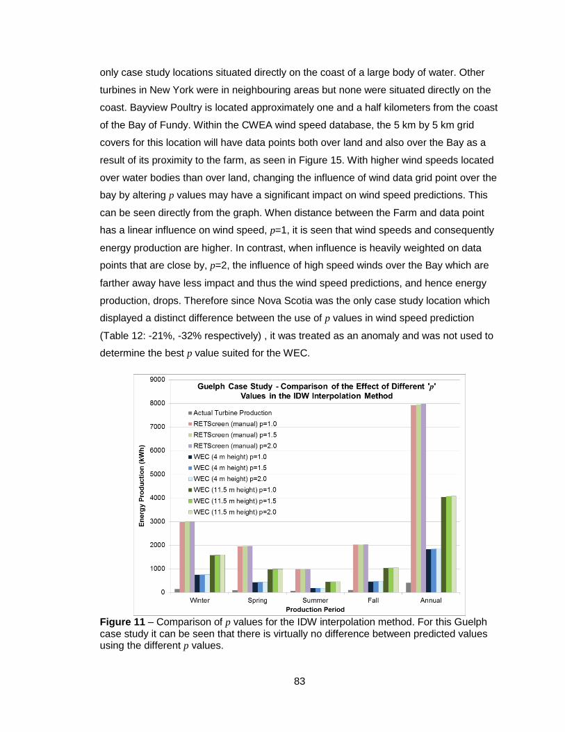
83

only case study locations situated directly on the coast of a large body of water. Other

turbines in New York were in neighbouring areas but none were situated directly on the

coast. Bayview Poultry is located approximately one and a half kilometers from the coast

of the Bay of Fundy. Within the CWEA wind speed database, the 5 km by 5 km grid

covers for this location will have data points both over land and also over the Bay as a

result of its proximity to the farm, as seen in Figure 15. With higher wind speeds located

over water bodies than over land, changing the influence of wind data grid point over the

bay by altering p values may have a significant impact on wind speed predictions. This

can be seen directly from the graph. When distance between the Farm and data point

has a linear influence on wind speed, p=1, it is seen that wind speeds and consequently

energy production are higher. In contrast, when influence is heavily weighted on data

points that are close by, p=2, the influence of high speed winds over the Bay which are

farther away have less impact and thus the wind speed predictions, and hence energy

production, drops. Therefore since Nova Scotia was the only case study location which

displayed a distinct difference between the use of p values in wind speed prediction

(Table 12: -21%, -32% respectively) , it was treated as an anomaly and was not used to

determine the best p value suited for the WEC.

Figure 11 – Comparison of p values for the IDW interpolation method. For this Guelph case study it can be seen that there is virtually no difference between predicted values using the different p values.

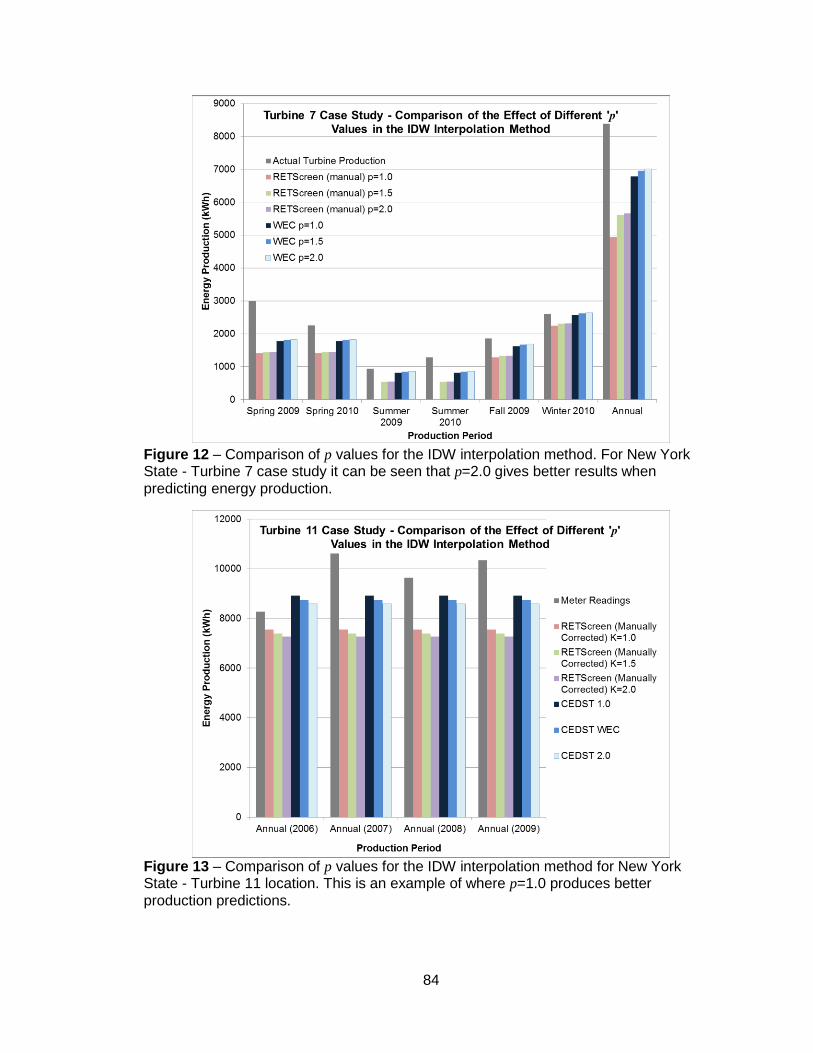
84

Figure 12 – Comparison of p values for the IDW interpolation method. For New York State - Turbine 7 case study it can be seen that p=2.0 gives better results when

predicting energy production.

Figure 13 – Comparison of p values for the IDW interpolation method for New York State - Turbine 11 location. This is an example of where p=1.0 produces better

production predictions.

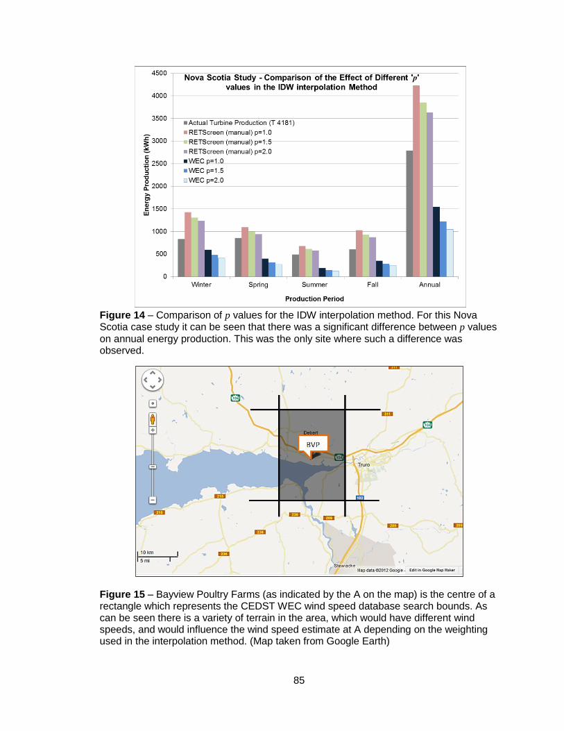
85

Figure 14 – Comparison of p values for the IDW interpolation method. For this Nova Scotia case study it can be seen that there was a significant difference between p values

on annual energy production. This was the only site where such a difference was observed.

Figure 15 – Bayview Poultry Farms (as indicated by the A on the map) is the centre of a rectangle which represents the CEDST WEC wind speed database search bounds. As can be seen there is a variety of terrain in the area, which would have different wind speeds, and would influence the wind speed estimate at A depending on the weighting used in the interpolation method. (Map taken from Google Earth)

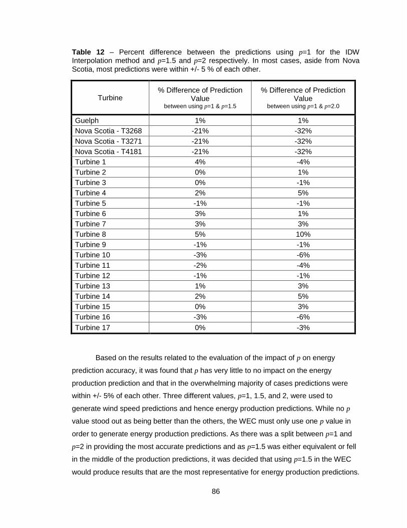
86

Table 12 – Percent difference between the predictions using p=1 for the IDW Interpolation method and p=1.5 and p=2 respectively. In most cases, aside from Nova

Scotia, most predictions were within +/- 5 % of each other.

Turbine % Difference of Prediction

Value between using p=1 & p=1.5

% Difference of Prediction Value

between using p=1 & p=2.0

Guelph 1% 1%

Nova Scotia - T3268 -21% -32%

Nova Scotia - T3271 -21% -32%

Nova Scotia - T4181 -21% -32%

Turbine 1 4% -4%

Turbine 2 0% 1%

Turbine 3 0% -1%

Turbine 4 2% 5%

Turbine 5 -1% -1%

Turbine 6 3% 1%

Turbine 7 3% 3%

Turbine 8 5% 10%

Turbine 9 -1% -1%

Turbine 10 -3% -6%

Turbine 11 -2% -4%

Turbine 12 -1% -1%

Turbine 13 1% 3%

Turbine 14 2% 5%

Turbine 15 0% 3%

Turbine 16 -3% -6%

Turbine 17 0% -3%

Based on the results related to the evaluation of the impact of p on energy

prediction accuracy, it was found that p has very little to no impact on the energy

production prediction and that in the overwhelming majority of cases predictions were

within +/- 5% of each other. Three different values, p=1, 1.5, and 2, were used to

generate wind speed predictions and hence energy production predictions. While no p

value stood out as being better than the others, the WEC must only use one p value in

order to generate energy production predictions. As there was a split between p=1 and

p=2 in providing the most accurate predictions and as p=1.5 was either equivalent or fell

in the middle of the production predictions, it was decided that using p=1.5 in the WEC

would produce results that are the most representative for energy production predictions.

87

As a result, p=1.5 will be used in the IDW interpolation method when generating wind

speed production predictions for the site of interest. This result is somewhat consistent

to results seen in literature, though the results are completely dependent on specific

location and use of the interpolated wind speed. A study performed by Stepek and

Wijnant (2011) compared p values of 0.5, 1, 2, 4, and 8, and found that p=2 gave the

best results for both surface and macro wind speed estimation. Similarly, Qian et al.

(2005) also found p=2 to be optimal.

11.3 Guelph

The Emergency Services Centre (ESC) located on Clair Road, officially opened in

Guelph, Ontario on June 20, 2011 (CoG 2011). As part of the Leadership in Energy and

Environmental Design (LEED) silver certification (CoG 2011), the roof of the ESC hosts

a 6.6 kW Wind Simplicity ‘Windancer7’ which was commissioned in April 2011 (Balean

2012). The turbine is located on the highest roof section on top of a 4 m tower designed

specifically by Wind Simplicity for use on flat roofs (WS 2008).

This was the only location obtained in Ontario that had available and useful wind

energy production data for a small turbine to be used as a case study for this work.

Although it offered sufficient energy production information, the turbine was not ideally

situated, being on a short tower on top of an approximately 7.5 m roof, to reflect the

production that would be expected for a turbine located on a taller tower on an

agricultural property. None-the-less, data was collected and evaluated to extract any

observable trends.

As can be seen from Figure 16, all of seasonal energy production predictions are

significantly higher than the actual production by the turbine. There are a few factors that

add inaccuracy into the predictions, though none are substantial enough to account for

such a large discrepency. One of these factors is that the power curve used in the WEC

is not the power curve for the Windancer 7 turbine. Wind Simplicity does not publish

power curves for their turbines and, when requested, the response was that there was

none available at the time. As a result, a power curve for a similar size of turbine, the

Eoltec SAS Scirocco ES 6.6 kW, was used (Eoltec SAS 2008). This turbine has the

same rated capacity as the Windancer7 but assumes a 24 m tower height in

calculations.

88

Tower height also plays a role in the WEC predictions. With a turbine situated on

a roof, the turbine tower height alone does not accurately reflect the height of the turbine

hub height or winds it is exposed to and hence the building height should be take into

account. Using the building (7.5 m) and tower (4 m) heights, the wind energy predictions

were performed using a 11.5 m hub height. Examing the results demonstrated that the

11.5 m hub height approximation generated predictions that were significantly greater

than actual turbine production (see Figure 16). Another case was performed as a ‘worst-

case’ scenario, using only the 4 m tower height as the hub height in the WEC prediction.

Again, it was seen that there was still a significant over-prediction even with the reduced

tower height.

Power curves can have an impact on overall power production, but since the

power curve was for an identically rated turbine and most wind turbine power curves are

qualitatively similar, the differences should not be as significant as observed with the

Guelph turbine. Additionally, of the two tower height scenarios, at least one should have

been able to realistically portray the turbine production or act as a lower and upper

bound for what the turbine could be expected to produce. As this was not the case, the

low energy production of the turbine must be attributed to other factors. Turbulence was

not accounted for in the WEC prediction and is an element that could have resulted in

the poor energy production. The wind flow entering the turbine’s sweep area would be

significantly disturbed by the roof geometry surrounding it as the turbine’s height above

the roof was not enough to bypass the turblence or allow the wind to regain a stable flow

pattern after being disrupted by the roof edge. As well, there is also the possibility that

the turbine itself, while rated at a specific power output, is not designed sufficiently as to

meet power projections in such a location.

89

Figure 16 – Case study relating the actual Guelph Windancer7 Turbine energy production to predictions made by the Wind Energy Calculator (at two different hub heights) and RETScreen (in both default and manually corrected scenarios). As can be seen, WEC predictions are more accurate related to the actual production, but all prediction scenarios severely over-predict actual production.

Due to the extremely poor relation between actual turbine energy production and

predictions generated by the prediction tools, estimated at 925% difference (Table 13),

and with many other confounding factors contributing to the uncertainty, this case study

was deemed not appropriate to be used to evaluate the performance of the WEC. Had

many of the other case studies had exhibited similar deviations, then conclusions could

be made on WEC prediction accuracy, but this was the only case where a deviation of

this magnitude occured and therefore demonstrates that it was an anomaly. What can

be seen from this study is that there is the potential for roof top turbines to perform

signficantly worse than predicted, as it is hard to incorporate the changes in speed and

turbulence in the wind flow as it passes over the roof.

As most farmers investigating the wind energy potential of their property would

not be looking to install a roof mounted turbine, but rather turbines mounted on the

ground, the dismissal of this case study does not impact the validation of the WEC in

situations where it would actually be used to make predictions.

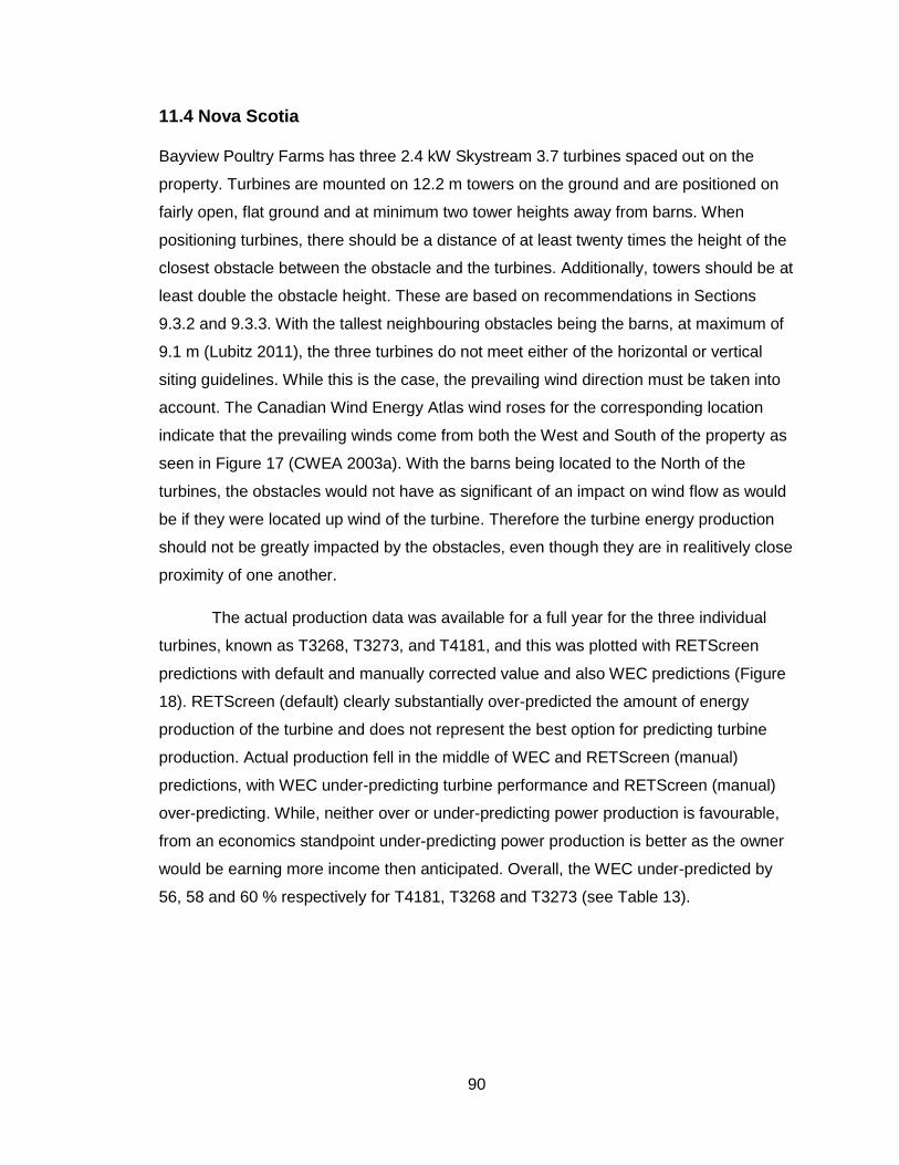
90

11.4 Nova Scotia

Bayview Poultry Farms has three 2.4 kW Skystream 3.7 turbines spaced out on the

property. Turbines are mounted on 12.2 m towers on the ground and are positioned on

fairly open, flat ground and at minimum two tower heights away from barns. When

positioning turbines, there should be a distance of at least twenty times the height of the

closest obstacle between the obstacle and the turbines. Additionally, towers should be at

least double the obstacle height. These are based on recommendations in Sections

9.3.2 and 9.3.3. With the tallest neighbouring obstacles being the barns, at maximum of

9.1 m (Lubitz 2011), the three turbines do not meet either of the horizontal or vertical

siting guidelines. While this is the case, the prevailing wind direction must be taken into

account. The Canadian Wind Energy Atlas wind roses for the corresponding location

indicate that the prevailing winds come from both the West and South of the property as

seen in Figure 17 (CWEA 2003a). With the barns being located to the North of the

turbines, the obstacles would not have as significant of an impact on wind flow as would

be if they were located up wind of the turbine. Therefore the turbine energy production

should not be greatly impacted by the obstacles, even though they are in realitively close

proximity of one another.

The actual production data was available for a full year for the three individual

turbines, known as T3268, T3273, and T4181, and this was plotted with RETScreen

predictions with default and manually corrected value and also WEC predictions (Figure

18). RETScreen (default) clearly substantially over-predicted the amount of energy

production of the turbine and does not represent the best option for predicting turbine

production. Actual production fell in the middle of WEC and RETScreen (manual)

predictions, with WEC under-predicting turbine performance and RETScreen (manual)

over-predicting. While, neither over or under-predicting power production is favourable,

from an economics standpoint under-predicting power production is better as the owner

would be earning more income then anticipated. Overall, the WEC under-predicted by

56, 58 and 60 % respectively for T4181, T3268 and T3273 (see Table 13).

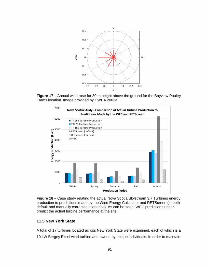
91

Figure 17 – Annual wind rose for 30 m height above the ground for the Bayview Poultry Farms location. Image provided by CWEA 2003a.

Figure 18 – Case study relating the actual Nova Scotia Skystream 3.7 Turbines energy production to predictions made by the Wind Energy Calculator and RETScreen (in both default and manually corrected scenarios). As can be seen, WEC predictions under-predict the actual turbine performance at the site.

11.5 New York State

A total of 17 turbines located across New York State were examined, each of which is a

10 kW Bergey Excel wind turbine and owned by unique individuals. In order to maintain

92

confidentiality of the turbine owners and their addresses, the turbines will be identified by

numbers based on site location (see Figure 10 which gives the labels and approximate

location of the turbine sites within the state).

As each turbine was installed on different dates and owned and operated by

different individuals, the period over which energy production was monitored and

recorded varied for each turbine. Data collection periods ranged between 2006 to 2011.

Seasonal energy production was extracted from the monthly averages calculated from

raw data that had been supplied (Section 10.1.3). Seasonal and annual energy

production were grouped according the the following method and the production values

were plotted alongside energy production predictions generated by RETScreen (default),

RETScreen (manual) corrected, and the WEC.

- Winter = December, January, February

- Spring = March, April, May

- Summer = June, July, August

- Fall = September, October, November

- Annual = Winter to Fall = December to November

This grouping method for the seasons was used as it agrees with the time period of the

seasonal wind speed data used in the WEC. Annual production was only calculated for

turbines where data existed for the 12 consecutive months. Thus, if data existed for

example December 2009 to April 2011, only one annual production total was calculated

(Annual 2010 = December 2009 to November 2010), and the remaining few months

were not added into the total.

The graphs for the 17 different wind turbines demonstrated a wide range of

correlations between actual energy production and energy predicitons. Predictions

ranged from under-predicting, to being in agreement with, to over-predicting compared

to the actual monitored production of the turbines. These correlations are demonstrated

in the respective graphs, Figure 19, Figure 20, and Figure 21, and the turbine case

studies were selected based on their representation of results. A complete set of graphs

for the remaining New York State wind turbines can be found in the Appendix A, Figure

24 - Figure 37.

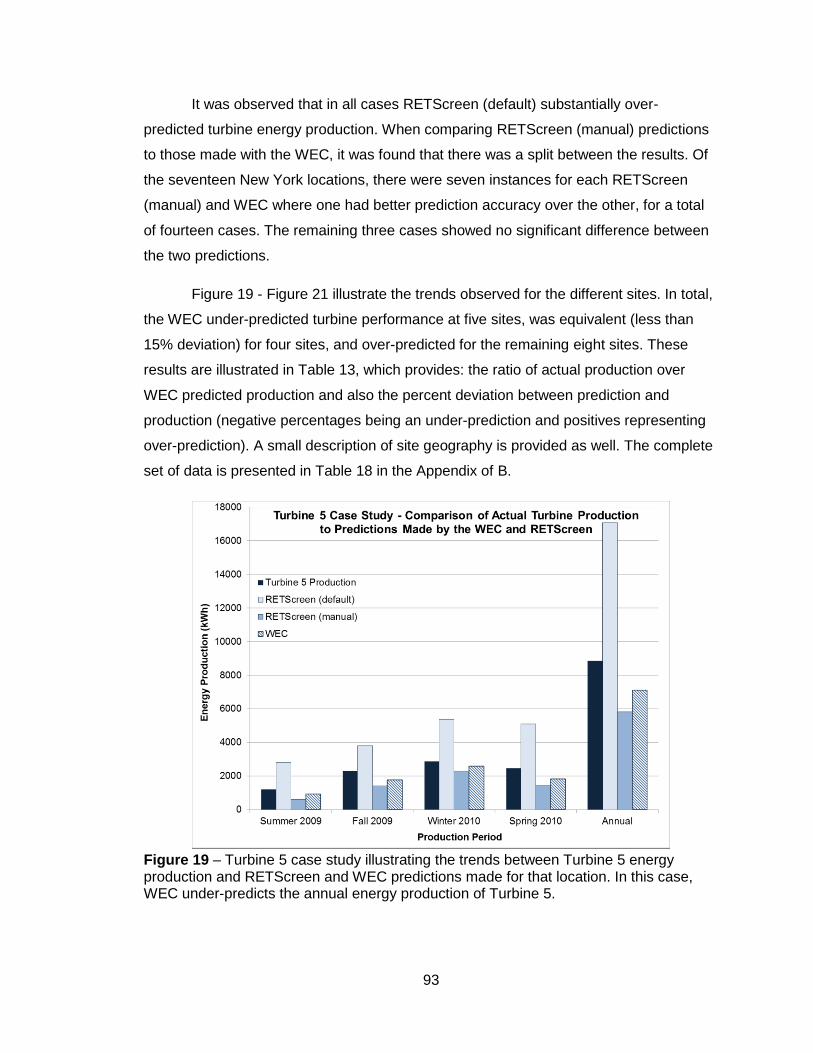
93

It was observed that in all cases RETScreen (default) substantially over-

predicted turbine energy production. When comparing RETScreen (manual) predictions

to those made with the WEC, it was found that there was a split between the results. Of

the seventeen New York locations, there were seven instances for each RETScreen

(manual) and WEC where one had better prediction accuracy over the other, for a total

of fourteen cases. The remaining three cases showed no significant difference between

the two predictions.

Figure 19 - Figure 21 illustrate the trends observed for the different sites. In total,

the WEC under-predicted turbine performance at five sites, was equivalent (less than

15% deviation) for four sites, and over-predicted for the remaining eight sites. These

results are illustrated in Table 13, which provides: the ratio of actual production over

WEC predicted production and also the percent deviation between prediction and

production (negative percentages being an under-prediction and positives representing

over-prediction). A small description of site geography is provided as well. The complete

set of data is presented in Table 18 in the Appendix of B.

Figure 19 – Turbine 5 case study illustrating the trends between Turbine 5 energy production and RETScreen and WEC predictions made for that location. In this case, WEC under-predicts the annual energy production of Turbine 5.

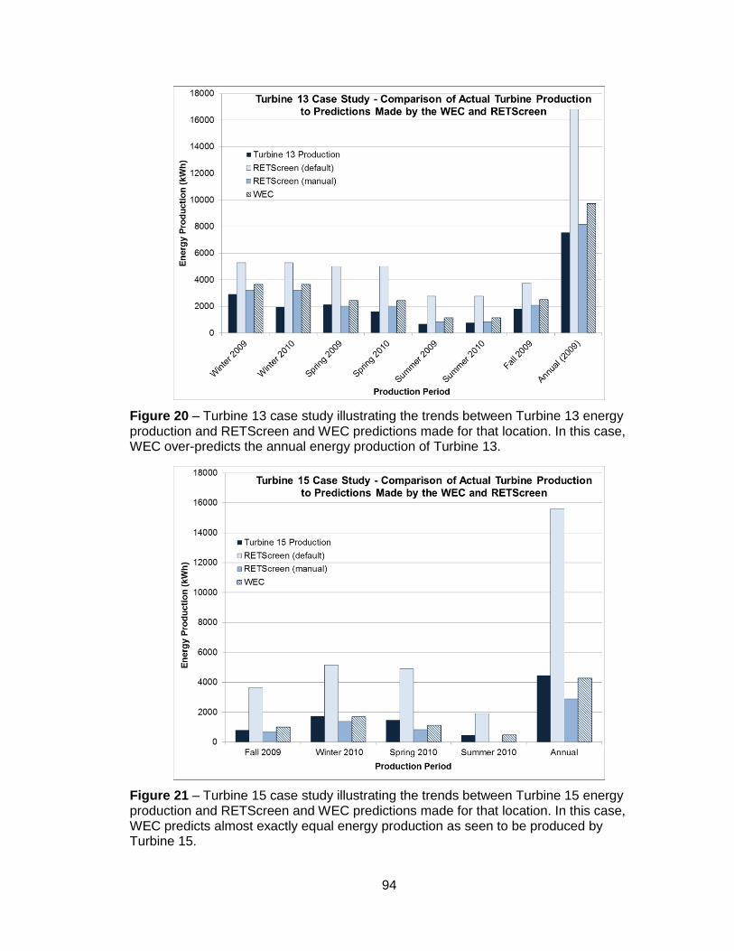
94

Figure 20 – Turbine 13 case study illustrating the trends between Turbine 13 energy production and RETScreen and WEC predictions made for that location. In this case, WEC over-predicts the annual energy production of Turbine 13.

Figure 21 – Turbine 15 case study illustrating the trends between Turbine 15 energy production and RETScreen and WEC predictions made for that location. In this case, WEC predicts almost exactly equal energy production as seen to be produced by Turbine 15.

95

Table 13 – Relationship between actual energy production of a turbine and what the turbine is anticipated to produce through ratio and percent deviation and also to site geography.

Ratio =

% Deviation =

(

)

Site Geography

Nova Scotia - T3271

2.71 -60% Flat, smooth land very

close to the Bay of Fundy

Nova Scotia - T3268



Nova Scotia - T4181



Turbine 16 1.67 -40% Flat with some

roughness

Turbine 9 1.30 -22% Small hilltop, larger surrounding hills,

relatively rough ground

Turbine 8 1.26 -20% Hillside

Turbine 5 1.24 -20% On a ridge top, ground

moderately rough around

Turbine 7 1.20 -17% Hillside

Turbine 11 1.11 -9% Ridge top (near a lake)

Turbine 15 1.04 -4% Hilltop, rough

surrounding ground

Turbine 14 0.93 8% Rough Ground

Turbine 3 0.88 14% Flat ground

Turbine 12 0.81 23% Hilltop, relatively rough

ground surrounding

Turbine 13 0.78 29% Hilly, rough ground

Turbine 6 0.75 33% Little hilltop, but much

lower than other hills, in a valley

Turbine 2 0.73 37% gradual sloping ground

Turbine 1 0.73 39% Flat

Turbine 10 0.68 49% Just off a ridge, flat

otherwise

Turbine 4 0.60 67% Flat

Turbine 17 0.44 127% Steep slopes, mountains

and valleys

Guelph 0.11 925% Rooftop of an urban

building

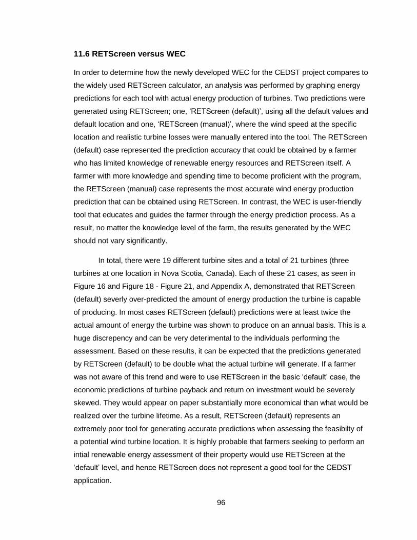
96

11.6 RETScreen versus WEC

In order to determine how the newly developed WEC for the CEDST project compares to

the widely used RETScreen calculator, an analysis was performed by graphing energy

predictions for each tool with actual energy production of turbines. Two predictions were

generated using RETScreen; one, ‘RETScreen (default)’, using all the default values and

default location and one, ‘RETScreen (manual)’, where the wind speed at the specific

location and realistic turbine losses were manually entered into the tool. The RETScreen

(default) case represented the prediction accuracy that could be obtained by a farmer

who has limited knowledge of renewable energy resources and RETScreen itself. A

farmer with more knowledge and spending time to become proficient with the program,

the RETScreen (manual) case represents the most accurate wind energy production

prediction that can be obtained using RETScreen. In contrast, the WEC is user-friendly

tool that educates and guides the farmer through the energy prediction process. As a

result, no matter the knowledge level of the farm, the results generated by the WEC

should not vary significantly.

In total, there were 19 different turbine sites and a total of 21 turbines (three

turbines at one location in Nova Scotia, Canada). Each of these 21 cases, as seen in

Figure 16 and Figure 18 - Figure 21, and Appendix A, demonstrated that RETScreen

(default) severly over-predicted the amount of energy production the turbine is capable

of producing. In most cases RETScreen (default) predictions were at least twice the

actual amount of energy the turbine was shown to produce on an annual basis. This is a

huge discrepency and can be very deterimental to the individuals performing the

assessment. Based on these results, it can be expected that the predictions generated

by RETScreen (default) to be double what the actual turbine will generate. If a farmer

was not aware of this trend and were to use RETScreen in the basic ‘default’ case, the

economic predictions of turbine payback and return on investment would be severely

skewed. They would appear on paper substantially more economical than what would be

realized over the turbine lifetime. As a result, RETScreen (default) represents an

extremely poor tool for generating accurate predictions when assessing the feasibilty of

a potential wind turbine location. It is highly probable that farmers seeking to perform an

intial renewable energy assessment of their property would use RETScreen at the

‘default’ level, and hence RETScreen does not represent a good tool for the CEDST

application.

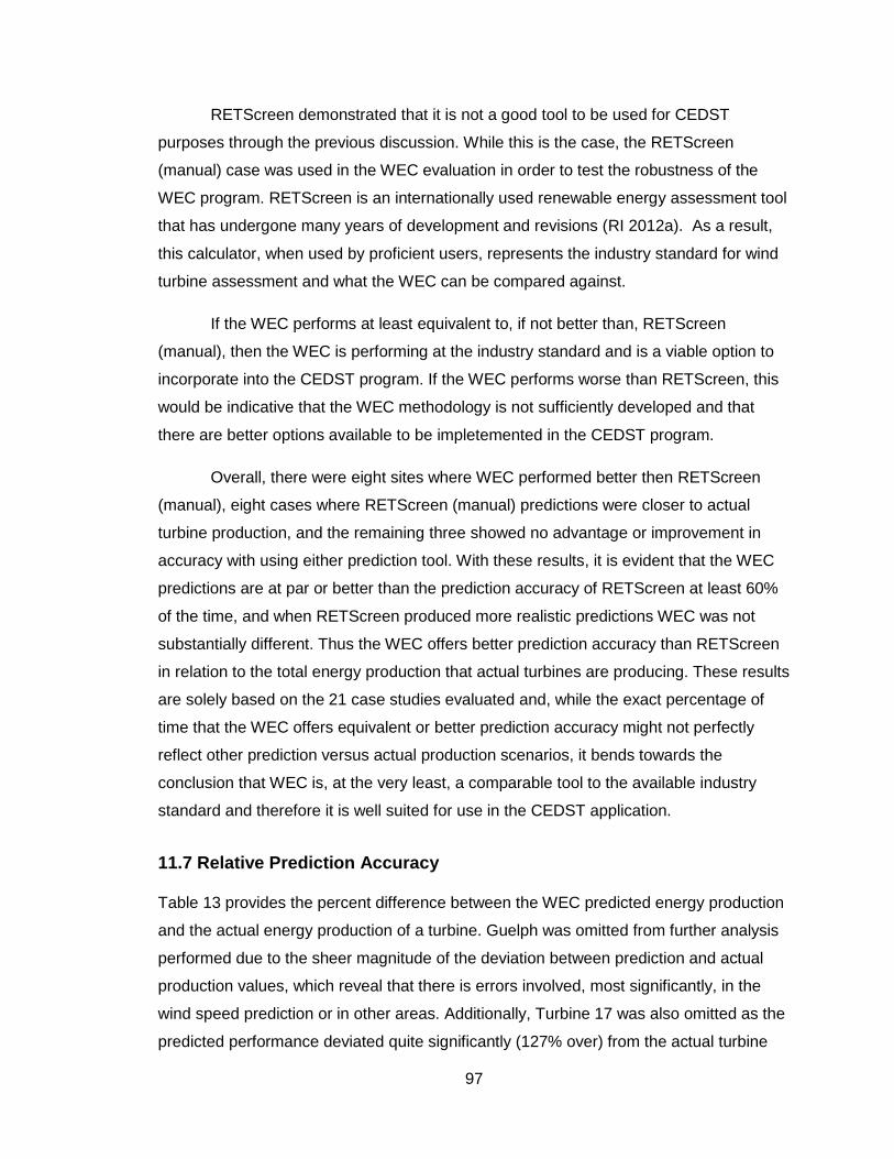
97

RETScreen demonstrated that it is not a good tool to be used for CEDST

purposes through the previous discussion. While this is the case, the RETScreen

(manual) case was used in the WEC evaluation in order to test the robustness of the

WEC program. RETScreen is an internationally used renewable energy assessment tool

that has undergone many years of development and revisions (RI 2012a). As a result,

this calculator, when used by proficient users, represents the industry standard for wind

turbine assessment and what the WEC can be compared against.

If the WEC performs at least equivalent to, if not better than, RETScreen

(manual), then the WEC is performing at the industry standard and is a viable option to

incorporate into the CEDST program. If the WEC performs worse than RETScreen, this

would be indicative that the WEC methodology is not sufficiently developed and that

there are better options available to be impletemented in the CEDST program.

Overall, there were eight sites where WEC performed better then RETScreen

(manual), eight cases where RETScreen (manual) predictions were closer to actual

turbine production, and the remaining three showed no advantage or improvement in

accuracy with using either prediction tool. With these results, it is evident that the WEC

predictions are at par or better than the prediction accuracy of RETScreen at least 60%

of the time, and when RETScreen produced more realistic predictions WEC was not

substantially different. Thus the WEC offers better prediction accuracy than RETScreen

in relation to the total energy production that actual turbines are producing. These results

are solely based on the 21 case studies evaluated and, while the exact percentage of

time that the WEC offers equivalent or better prediction accuracy might not perfectly

reflect other prediction versus actual production scenarios, it bends towards the

conclusion that WEC is, at the very least, a comparable tool to the available industry

standard and therefore it is well suited for use in the CEDST application.

11.7 Relative Prediction Accuracy

Table 13 provides the percent difference between the WEC predicted energy production

and the actual energy production of a turbine. Guelph was omitted from further analysis

performed due to the sheer magnitude of the deviation between prediction and actual

production values, which reveal that there is errors involved, most significantly, in the

wind speed prediction or in other areas. Additionally, Turbine 17 was also omitted as the

predicted performance deviated quite significantly (127% over) from the actual turbine

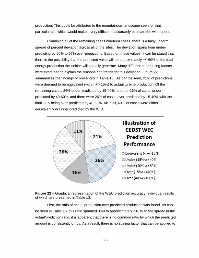
98

production. This could be attributed to the mountainous landscape seen for that

particular site which would make it very difficult to accurately estimate the wind speed.

Examining all of the remaining cases nineteen cases, there is a fairly uniform

spread of percent deviation across all of the sites. The deviation spans from under-

predicting by 60% to 67% over-predictions. Based on these values, it can be stated that

there is the possibility that the predicted value will be approximately +/- 60% of the total

energy production the turbine will actually generate. Many different contributing factors

were examined to explain the reasons and trends for this deviation. Figure 22

summarizes the findings of presented in Table 13. As can be seen, 21% of predictions

were deemed to be equivalent (within +/- 15%) to actual turbine production. Of the

remaining cases, 26% under-predicted by 15-40%, another 16% of cases under-

predicted by 40-60%, and there were 26% of cases over-predicted by 15-40% with the

final 11% being over-predicted by 40-60%. All in all, 63% of cases were either

equivalently or under-predicted by the WEC.

Figure 22 – Graphical representation of the WEC prediction accuracy, individual results of which are presented in Table 13.

First, the ratio of actual production over predicted production was found. As can

be seen in Table 13, this ratio spanned 0.60 to approximately 3.0. With the spread in the

actual/prediction ratio, it is apparent that there is no common ratio by which the predicted

amount is consistently off by. As a result, there is no scaling factor that can be applied to

99

the general equation to help minimize the deviation between the predicted production

and what would actually be seen.

Each of the case studies spanned various time periods. Data for New York State

ranged from 2006 to 2011. Additionally, in Nova Scotia the turbines were monitored

between 2009 and 2010, and in Ontario the turbine data was recorded from 2011 to

2012. Timeframe is important because, since the wind speed database is based off of a

43 year averaging period, the data used for wind speed prediction is representative of an

‘average wind speed year’, but the year the data was collected might not have been an

‘average wind speed year’. When examining the New York State data in Figure 19-

Figure 21 and Figure 24-Figure 37, seasonal and annual under and over-predictions

were identified, along with the time they occurred. Comparing timeframes of under or

over-predictions from one turbine to another found that there were no years, or even

seasons within a year, that could be identified as consistently under or over-predicting.

With no consistent trends in under or over-predictions, it was not possible to correlate

this with either lower or higher seasonal and annual wind speeds.

The wind speeds were obtained for the monitored years for Nova Scotia and

Ontario respectively (WSoLYfT 2012, WSoLYfG 2012) and compared to the average

wind speeds produced by the database interpolation. Wind speeds were taken from

Environment Canada (WSoLYfT 2012, WSoLYfG 2012) for the monitoring locations

closest to the turbine sites; Truro, NS for Bayview Poultry and Guelph for the Guelph

turbine. The data provided was then averaged to get an annual average and, with

Guelph, it was possible to find the annual average over the period turbine data was

recorded over. These were the Enivoronment Canada annual averages representing

actually observed wind speeds at the sites. These values were then compared to the

wind speeds used in the CEDST WEC program to generate the feasibility assessments.

CEDST WEC annual average wind speed data was provided at 30 m and 50 m. The

wind shear exponent was found for this height range (Equation 8), and was then applied

to estimate the wind speed at 10 m using Equation 9, as was the height of Environment

Canada wind speed measurements (EC 2012b). Using the wind shear exponent found

for the 30-50 m range to calculate the wind speed at 10 m is not entirely correct but was

the best option with the available information.

100

As can be seen in Table 14 WEC wind speeds were slightly lower and higher

then the winds actually seen on site for Nova Scotia and Guelph respectively. The low or

high wind speed values used in the WEC could be a contributing factor for the under and

over-predictions of site energy production for their corresponding location. Though this

may be the case the 0.47 m/s over estimate of the wind speed at Guelph would not have

been enough to account for the extremely large over-prediction of energy production and

thus other factors, such as the roof-top location of the turbine, must play a large role in

accounting for the deviation. It must also be noted that both sites only recorded data for

a single year so it is reasonable to anticipate that wind speeds may slightly different than

the annual average.

Table 14 – Comparison of wind speeds used in the CEDST WEC to those from Environment Canada monitoring sites

Data Source Wind Speed (m/s)

Masstown, Nova Scotia

CEDST WEC 3.50

Truro, NS - Environment Canada (EC) (2.5 year average) 3.62

Difference Between WEC and EC -0.12

Guelph, Ontario

CEDST WEC 3.61

Guelph, ON - Environment Canada (over recording period) 3.14

Guelph, ON - Environment Canada (5 year average) 3.36

Difference Between WEC and EC (recording period) 0.47

Overall, it appeared that the wind speeds being used in the WEC prediction were

representative of the wind speeds being observed at the turbine sites and therefore

deviation between prediction and actual production cannot be solely attributed to higher

or lower then average wind speeds.

An additional factor that was evaluated was the terrain of the wind turbine site

and surrounding area to see if it was possible to identify geographical features that were

consistently contributing to the deviation of the predictions to the actual turbine

production. The terrain for each of the sites was viewed on a elevation maps and

through Google Earth and is briefly described in Table 13. There was a wide range of

geographical features for the turbine sites including; flat ground, smooth rolling hills,

ridges, and coastal areas. For example, the table reveals that it is possible for a very flat

101

location to have both under (Turbine 16) and over-predictions (Turbine 4). The

inconsistency of deviation with respect to terrain type makes it hard to draw any

conclusions as to why certain sites experienced either under or over-predictions. Based

on these results, there is no relationship between the site geographical features and

whether the WEC will predict higher or lower energy production to what a turbine at the

site would actually produce.

11.8 Case Study Conclusions

Overall there were 21 turbines used as case studies. Though the case studies showed

varying results, there are some general trends that were able to be derived from the

work.

First is that the studies illustrated that there is very little influence of the p

influence factor used in the IDW interpolation method. After having investigated p= 1,

1.5, and 2, cases were split between having p=1 being better, p=2 being better, or

having no difference between the two. Since p=1.5 results were normally nearly

equivalent to p=1 or p=2, or fell directly in the middle of the two, it was determined that

using p=1.5 in the WEC IDW interpolation method would give the best average results.

It was also found that RETScreen (default) significantly over-predicted the

production that an actual turbine is capable of producing. As a result, RETScreen should

only be used by individuals who are knowledgeable in the renewable energy field and

are skilled at using the program. If used by individuals lacking knowledge or familiarity of

the program, RETScreen will undoubtedly produce highly unrealistic economic

predictions for a wind turbine project and cause the user to not realize the economic

potential of what had originally been predicted.

Comparison of WEC to RETScreen (manual) was done to examine the

performance of the WEC tool in relation to the industry standard. It was seen that of the

nineteen sites, eleven (approximately 60%) were instances when WEC generated

predictions which were at par or better than RETScreen predictions.

There was a wide range of prediction accuracy when examining WEC predictions

to actual production of existing turbines. The Guelph case study proved to be an

anomaly of all the cases as it had the greatest deviation between predicted and

produced energy, potentially attributed to the rooftop placement of the turbine. As an

102

anomaly, the Guelph case study was omitted when observing trends within the cases.

Additionally, Turbine 17 was also omitted when looking at the relative prediction

accuracy due to its location within a mountainous region making it difficult to estimate

wind speeds. Though there was a wide range in prediction accuracy of the nineteen

cases, the spread was fairly uniform and had upper and lower bounds of approximately

+/- 60%. A total of 21% of predictions were deemed to be equivalent to the actual energy

produced, 42% under-predicted, the remaining 37% were over-predictions. The even

spread of under or over-predictions reveals that there is no systematic error internal to

the WEC program which would cause a consistent bias of results. As a result, the

deviation between predictions and actual production is attributed to other sources of

error. Though this is the case, the economic impact of such under or over-prediction

percentage is presented in the up-coming chapter.

Both actual wind speed and terrain were investigated to see if they could explain

the deviation observed between the WEC predictions and actual turbine production.

Seasonal and annual wind speeds seen at the turbines sites over the data recording

period were not shown to be significantly different from the WEC predicted wind speeds.

As a result, the WEC wind speed data seems to be in line with actually occurring wind

speeds. There was a wide variety of terrain types and these site geographies did not

show a trend between terrain and whether the WEC under or over-predicted. For

example, sites having a flat geography represented some of the extremes in both under

and over-predictions made by the WEC.

103

Chapter 12 – Examination of WEC Economic Results

12.1 Introduction and Normal WEC Economic Predictions

Calculation of wind turbine power production does not constitute a complete feasibility

assessment. Power production, along with project expenses, must then be used to

calculate the cash flow for the project. Power production is based off seasonal average

wind speed data, and is assumed to be the same value every year of the project lifetime.

This amount is multiplied by the tariff rate or consumer electricity price to represent the

annual revenue or savings respectively.

For all 10 kW Bergey Excel turbine case studies the WEC produced power

production predictions based on the average site wind speed estimates. The predicted

production values were then used for each year of the turbine lifetime to generate a cash

flow graph and feasibility assessment. It was assumed that the turbine was part of the

FIT program, the entire cost of was paid upfront (no financing), and also that there were

no yearly operational and maintenance expenses. All of the variables were entered into

the WEC and it produced an economic assessment of each site.

All case study sites used in this thesis underwent a WEC economic assessment,

in addition to the generation of power production results, as the main purpose of the

WEC program is to evaluate the economic feasibility of sites. Power production was the

only means of testing the accuracy and reliability of the WEC program, though probably

the most accurate, since only production data was recorded for each turbine and there

was no indication to any of the costs or economics associated with them. Only when all

economic variables are known and able to be entered into the WEC, would it be possible

to compare the economic prediction to what was seen in real life. Instead, since

economics relies directly on power production, if power production predictions were

shown to be accurate it follows that the economics will be also.

As there are no actual economic data for the case studies, this chapter will solely

use the sites and turbine models to generate the predicted feasibility of each turbine

case study project. Two sites were selected from the seventeen locations in New York

State to be presented. The sites of turbines 16 and 17 were chosen as they represented

the extreme cases of power prediction accuracy being 40% under and 127% over the

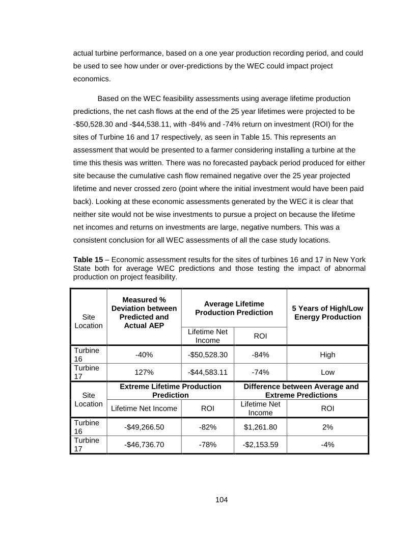
104

actual turbine performance, based on a one year production recording period, and could

be used to see how under or over-predictions by the WEC could impact project

economics.

Based on the WEC feasibility assessments using average lifetime production

predictions, the net cash flows at the end of the 25 year lifetimes were projected to be

-$50,528.30 and -$44,538.11, with -84% and -74% return on investment (ROI) for the

sites of Turbine 16 and 17 respectively, as seen in Table 15. This represents an

assessment that would be presented to a farmer considering installing a turbine at the

time this thesis was written. There was no forecasted payback period produced for either

site because the cumulative cash flow remained negative over the 25 year projected

lifetime and never crossed zero (point where the initial investment would have been paid

back). Looking at these economic assessments generated by the WEC it is clear that

neither site would not be wise investments to pursue a project on because the lifetime

net incomes and returns on investments are large, negative numbers. This was a

consistent conclusion for all WEC assessments of all the case study locations.

Table 15 – Economic assessment results for the sites of turbines 16 and 17 in New York State both for average WEC predictions and those testing the impact of abnormal production on project feasibility.

Site

Location

Measured % Deviation between

Predicted and Actual AEP

Average Lifetime Production Prediction

5 Years of High/Low Energy Production

Lifetime Net

Income ROI

Turbine 16

-40% -$50,528.30 -84% High

Turbine 17

127% -$44,583.11 -74% Low

Site Location

Extreme Lifetime Production Prediction

Difference between Average and Extreme Predictions

Lifetime Net Income ROI Lifetime Net

Income ROI

Turbine 16

-$49,266.50 -82% $1,261.80 2%

Turbine 17

-$46,736.70 -78% -$2,153.59 -4%

105

12.2 Impacts of Abnormal Wind Production

The sites of Turbine 16 and 17 were selected based on the fact that they represented

the bounds on WEC accuracy. This means that over the period of data collection actual

production from the turbines at this site did not match what the WEC predicted.

It would be a normal occurrence for the actual annual energy production to

deviate slightly from the projected production, as different years will see slight variations

from annual average wind speeds. On average though, over the 25 year turbine lifetime,

it would be assumed that years with higher and lower energy production would balance

out and the lifetime production would be fairly representative of WEC predictions using

an average annual energy production (AEP).

Turbines 16 and 17 each only had one year of data collection. Though the AEP

recorded for the turbines were significantly higher and lower respectively, compared to

the AEP predicted by the WEC, a single year of data is not enough to establish any long

range trends. A single year of abnormal energy production cannot be considered

representative of the lifetime production of a turbine. Therefore these sites could see

future years with opposite energy production (lower for site 16 and higher for site 17)

that would average out the effects of the year of recorded data and turbines could still be

consistent with WEC predictions for lifetime energy production.

The inaccuracies between predicted and actual AEP for seen for sites 16 and 17

bring light to a thought about the impact this could have on overall project economics,

even if it is assumed that high and low AEP will balance out over a turbine lifetime.

CWEA data is based on 43 years of data modelling, taking into account annual

variations, and should be representative of average wind speeds seen at a site over 25

years, the lifetime of a turbine. However, supposing a site had abnormally high or low

wind speeds for a fraction of this time, would this cause significant differences between

predicted and actual wind turbine project economics?

This was question was evaluated for both sites 16 and 17. For investigation

purposes, it was assumed that the sites would see five years off abnormal AEP

(consistent with the actual AEP recorded for Turbines 16 and 17) and the other 20 years

being consistent with the average AEP predicted with the WEC. Five years was selected

as it represents a reasonable fraction of the turbine’s life that would be able to have an

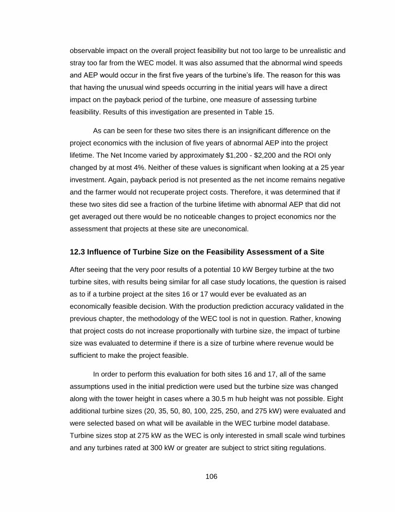
106

observable impact on the overall project feasibility but not too large to be unrealistic and

stray too far from the WEC model. It was also assumed that the abnormal wind speeds

and AEP would occur in the first five years of the turbine’s life. The reason for this was

that having the unusual wind speeds occurring in the initial years will have a direct

impact on the payback period of the turbine, one measure of assessing turbine

feasibility. Results of this investigation are presented in Table 15.

As can be seen for these two sites there is an insignificant difference on the

project economics with the inclusion of five years of abnormal AEP into the project

lifetime. The Net Income varied by approximately $1,200 - $2,200 and the ROI only

changed by at most 4%. Neither of these values is significant when looking at a 25 year

investment. Again, payback period is not presented as the net income remains negative

and the farmer would not recuperate project costs. Therefore, it was determined that if

these two sites did see a fraction of the turbine lifetime with abnormal AEP that did not

get averaged out there would be no noticeable changes to project economics nor the

assessment that projects at these site are uneconomical.

12.3 Influence of Turbine Size on the Feasibility Assessment of a Site

After seeing that the very poor results of a potential 10 kW Bergey turbine at the two

turbine sites, with results being similar for all case study locations, the question is raised

as to if a turbine project at the sites 16 or 17 would ever be evaluated as an

economically feasible decision. With the production prediction accuracy validated in the

previous chapter, the methodology of the WEC tool is not in question. Rather, knowing

that project costs do not increase proportionally with turbine size, the impact of turbine

size was evaluated to determine if there is a size of turbine where revenue would be

sufficient to make the project feasible.

In order to perform this evaluation for both sites 16 and 17, all of the same

assumptions used in the initial prediction were used but the turbine size was changed

along with the tower height in cases where a 30.5 m hub height was not possible. Eight

additional turbine sizes (20, 35, 50, 80, 100, 225, 250, and 275 kW) were evaluated and

were selected based on what will be available in the WEC turbine model database.

Turbine sizes stop at 275 kW as the WEC is only interested in small scale wind turbines

and any turbines rated at 300 kW or greater are subject to strict siting regulations.

107

Looking at the analysis results displayed in Table 16 it can be seen that the site

of turbine 16 is never a feasible project location no matter the size of the turbine

installed. This is similar to the results for the site of turbine 17, though the 35 kW turbine

did offer the closest scenario where the turbine would break-even (ROI = -4%).

Table 16 – Results of the economic assessments for sites 16 and 17 investigating how project feasibility changes with turbine size.

Economic Assessment of the Site of Turbine 16

Rated Power

Model Hub

Height Lifetime Net

Income ROI

10 Bergey Excel 10kW 30.5 -$ 50,528.33 -84%

20 ReDriven 20 24.4 -$ 94,540.41 -79%

35 Endurance Wind Power 35kW -

G3120 30.5 -$ 45,999.69 -40%


E3120 30.5 -$ 94,633.75 -57%

80 Wind Energy Solutions WES80 32 -$ 202,938.38 -77%

100 Northern Power 100 37 -$ 213,720.67 -65%

225 Aeronautica Windpower -

225kW 40 -$ 556,321.20 -75%


275 Vergnet GEV MP R 35.4 -$ 701,016.71 -77%


Rated Power

Model Hub

Height Lifetime Net

Income ROI

10 Bergey Excel 10kW 30.5 -$ 45,294.00 -75%

20 ReDriven 20 24.4 -$ 83,258.78 -69%


G3120 30.5 -$ 4,572.40 -4%


E3120 30.5 -$ 49,160.93 -30%


100 Northern Power 100 37 -$ 181,812.47 -55%


225kW 40 -$ 414,535.82 -56%


275 Vergnet GEV MP R 35.4 -$ 544,760.05 -60%

Neither site 16 or 17 demonstrated to be feasible options for turbine projects.

With these results, another site was examined to see if it would ever be possible for a

small wind turbine to be reasonably feasible. In order to determine which site to use a

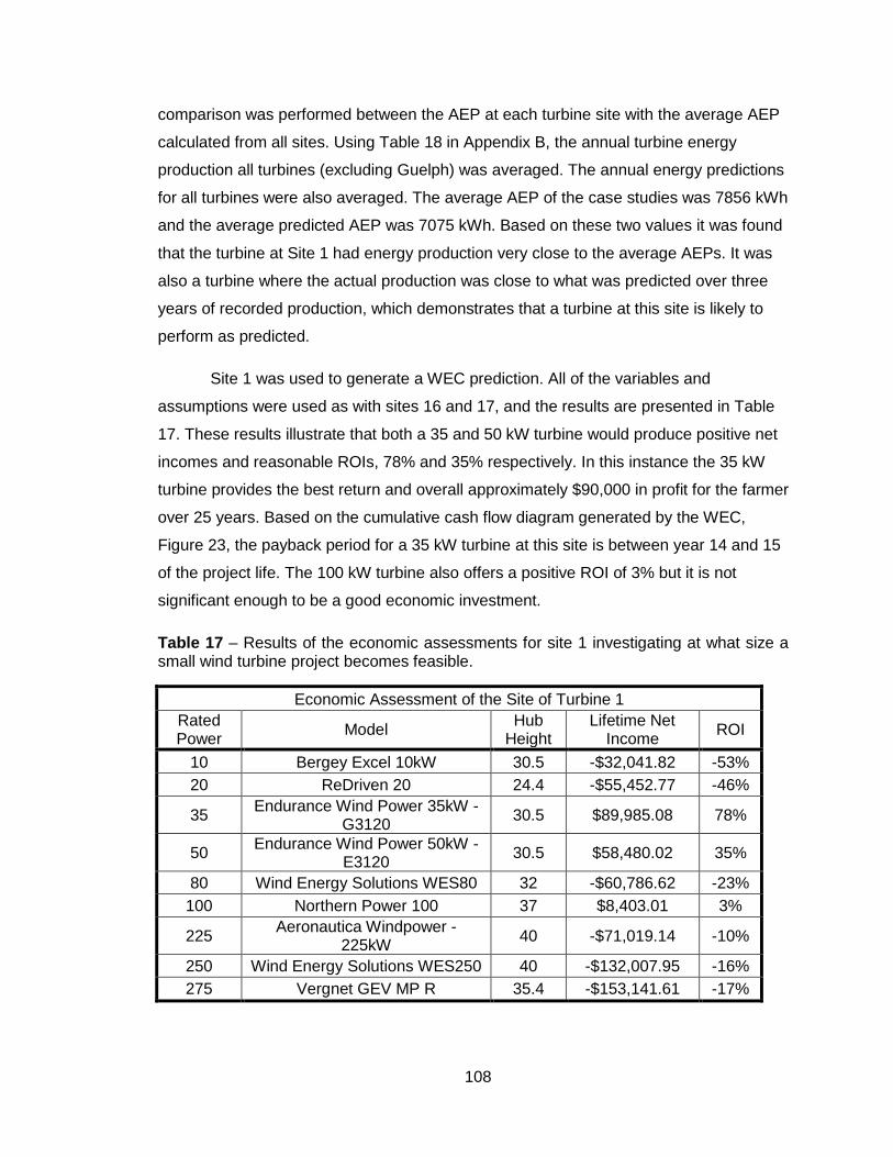
108

comparison was performed between the AEP at each turbine site with the average AEP

calculated from all sites. Using Table 18 in Appendix B, the annual turbine energy

production all turbines (excluding Guelph) was averaged. The annual energy predictions

for all turbines were also averaged. The average AEP of the case studies was 7856 kWh

and the average predicted AEP was 7075 kWh. Based on these two values it was found

that the turbine at Site 1 had energy production very close to the average AEPs. It was

also a turbine where the actual production was close to what was predicted over three

years of recorded production, which demonstrates that a turbine at this site is likely to

perform as predicted.

Site 1 was used to generate a WEC prediction. All of the variables and

assumptions were used as with sites 16 and 17, and the results are presented in Table

17. These results illustrate that both a 35 and 50 kW turbine would produce positive net

incomes and reasonable ROIs, 78% and 35% respectively. In this instance the 35 kW

turbine provides the best return and overall approximately $90,000 in profit for the farmer

over 25 years. Based on the cumulative cash flow diagram generated by the WEC,

Figure 23, the payback period for a 35 kW turbine at this site is between year 14 and 15

of the project life. The 100 kW turbine also offers a positive ROI of 3% but it is not

significant enough to be a good economic investment.

Table 17 – Results of the economic assessments for site 1 investigating at what size a small wind turbine project becomes feasible.


Rated Power

Model Hub

Height Lifetime Net

Income ROI

10 Bergey Excel 10kW 30.5 -$32,041.82 -53%

20 ReDriven 20 24.4 -$55,452.77 -46%


G3120 30.5 $89,985.08 78%


E3120 30.5 $58,480.02 35%

80 Wind Energy Solutions WES80 32 -$60,786.62 -23%

100 Northern Power 100 37 $8,403.01 3%


225kW 40 -$71,019.14 -10%

250 Wind Energy Solutions WES250 40 -$132,007.95 -16%

275 Vergnet GEV MP R 35.4 -$153,141.61 -17%

109

Figure 23 – Case flow diagram for a 35 kW turbine project assessed at site 1 in New York State. It was found that, assuming the turbine was part of the FIT program, the payback period for the turbine would be between year 15 and 16 of the project life.

The analysis of New York State Site 1 proves that it is possible for small wind

turbine projects to be feasible initiatives under the FIT program.

12.4 Interpretation of Results

With the three sites, 1, 16, and 17, in New York there were varied results in the feasibility

of small wind turbine projects. Site 16 revealed that no turbine sizes were feasible, Site

17 had the same result although the 35 kW turbine was almost at the break-even point

by the end of the project life and Site 1 illustrates that a small 35 kW turbine could

actually be a financially beneficial investment opportunity. All variables, other than

location, were kept constant between the case studies and as a result the variation in

economic results must be attributed to the location. Annual wind speeds for each of the

three sites, as predicted by the WEC, were collected and are as follows:

- Site 1 Annual Wind Speeds: 4.44 m/s at 30.5 m


110


As a result, location wind speed is directly related to the feasibility of a project since Site

1, with the highest wind speeds is a sound economic decision, whereas Site 16, with the

lowest winds, is not feasible. Thus, since Site 1 represented average AEP for all cases,

it would be assumed that sites with AEPs above average would have proportionally

better economic results with more turbine sizes becoming feasible and generating higher

net incomes and ROIs.

Another point of observation was that the feasibility of projects did not increase

with turbine size as was originally thought. There are two main reasons for this including

turbine power curves and turbine heights. Turbine power curves cut-in wind speeds were

explained in Section 6.4. Smaller turbines tend to have lower cut-in wind speeds. As a

result, even though a small turbine, e.g. 35 kW, will not generate as much power as a

larger turbine, e.g. 100 kW, it will start generating power at a lower wind speed. This is

important because the average wind speeds of the sites used in this study are

reasonably low and therefore represent the winds the turbine will be exposed to.

Additionally, the hub height was kept to approximately 30-40 m. This is

reasonably close to the ground where slower wind speeds are. Restricting the height of

the turbines limits the wind speeds the turbines see and thus limits the amount of power

produced.

12.5 Summary

Overall, it was found that the WEC is able to generate economic assessments of wind

turbine sites and provide information on cash flow diagrams, net income, and ROI. If

abnormal wind speeds were to occur over a fraction of the turbine life it will not

significantly impact the feasibility results. Additionally, though many of the sites showed

that small turbines would not be an economical investment, sites with higher wind

speeds and different turbine sizes represented highly feasible wind turbine project

investment opportunities.

111

Chapter 13 – Sources of Error

13.1 Sources of Error in WEC

As with any project, there are sources of error that can cause results and conclusions to

be skewed or biased. The CEDST WEC project is no exception. While the assumptions

and values used in the decision making process and calculations were explained in this

thesis, there is some inherent error that can make the WEC results not completely

accurate for every project a user wishes to assess.

13.1.1 Wind Speed Calculations

Within the process of calculating the site wind speed, there are a few areas where error

could have occurred. First, and most fundamental, is that the wind speed data used in

the database could be incorrect. Based on the average of 43 years (1958-2000) of wind

modelling, the CWEA data is the best source for the WEC database but does not

necessarily mean that these averages are realistic in representing an average year post

2000. Additionally, with only 5 km grid resolution, there can still be significant variation in

wind speed between data points. A more up-to-date and higher resolution database

would be best for the WEC application but, as stated, the CWEA was the best available.

The IDW interpolation method, with a p=1.5, was incorporated into the WEC. It

was the most applicable method found but, even as can be seen in the Nova Scotia

Case Study, there can be a wide variety in wind speed results depending on where grid

points are located. While this method was best for the overall WEC tool, there may be

error associated with the predictions the IDW interpolation method produces.

Once wind speed data was obtained at 30 and 50 m heights, the wind shear

exponent (α) was calculated. This exponent was then used, in conjunction with the 30 m

wind speed, to calculate the wind speed at hub height. Since the exponent was found

using 30 and 50 m data, it is most representative of the trend between these two

heights. If the hub height were, for example, 24 m above ground, the WEC still uses the

α calculated even though 24 m does not occur in the 30 to 50 m range. As a result, the

actual α for hub heights less than 30 m may be slightly different than what is used in

calculations and some error in wind speed predictions will result.

112

Finally, other than providing the siting regulations and making recommendations

for turbine placement, no micro-siting was incorporated into the calculations. It was

determined that to incorporate micro-siting calculations would be incredibly complex and

add more error and uncertainty into the WEC in comparison to the benefit it would add.

With micro-siting excluded there will be some inherent error in the WEC predictions

generated. An example of where the exclusion of micro-siting effects (such as

turbulence) on wind speed play an role is the Guelph Turbine Case Study, where

neglecting siting impacts on wind speed caused the WEC to generate severe over-

predictions compared to actual production. Though it is excluded, recommendations are

provided within the calculator to guide the user in micro-siting the turbine in order to help

maximize turbine performance.

Although these four factors will contribute error to the WEC predictions, it is very

hard to find other values or methods which are currently more accurate and can be

applied to a general calculator capable of easily assessing wind turbine projects across

Ontario with minimal user inputs. As a result, it would be impossible to remove all

sources of error while still maintaining the functionality of the calculator. Research was

performed in each area and the methodology decided upon for the WEC was based on

the best, most accurate, and most applicable results of this research.

13.1.2 Power Calculations

There are also sources of error within the power calculations. One such source is the

standard losses used within the WEC. As stated in Chapter 7.1, losses were assumed to

be: 0% array, 3% soiling and icing, 3% miscellaneous, and 5% downtime, and assumed

to be consistent across all turbine models for all time periods. These values were used

based on industry standards and also in an attempt to produce an accurate, but

conservative, feasibility prediction. In a real setting, there may be some changes in these

losses which would result in error in the WEC prediction. For example, if there are

multiple turbines on site the array losses would not necessarily be 0%.

Another assumption that could result in error was that the power curves for each

turbine model are representative and accurate. All manufacturers provided power curves

for their turbines. While it is expected that these published curves are accurate and have

been validated, there is the chance that the curves have not been tested or do not

accurately match the power curve of a turbine that would actually be installed. With an

113

inaccurate power curve, it would be impossible to accurately predict the wind turbine

feasibility. Though the chance for error in the power curves exists, it was necessary to

assume the manufacturers to be honest and true in the work they produce.

13.1.3 Economics

The WEC was designed to be a tool for assessment of turbines in the Province of

Ontario. As a result, interest rates, electricity prices, and the Feed-in Tariff rates

provided within the WEC are specific to this province. Setting these as the ‘default’

values allows for provincial assessments to be easily performed. While there are default

values, the user maintains the ability to manually change the rates to better represent

the economic variables specific to their location (outside of province) and project.

Additionally, turbine project costs are represented in Table 5 and Table 7 as

industry averages and price ranges depending on the size of turbine. Within the WEC,

project cost was approximated by using the price per kW specific to the size of turbine of

interest. Actual costs of the constructed project may vary from these values as they are

general averages. Similar to the above situation, the approximated cost of the turbine

will be provided as the default value within the WEC and the user could still enter in a

more accurate value if known.

13.2 Error Summary

Overall, there are many areas where error could occur in the WEC. Although the

sources of error have been identified, they have also been validated as to why the

values and methodology were incorporated into the WEC. Thus, though there may be

some inherent error in WEC predictions, the calculator methodology is robust and

represents the best possible methodology for performing wind energy predictions as of

the current day.

114

Chapter 14 – Conclusion

The overall goal of this project was to develop a wind energy prediction calculator that

could be implemented into the Complimentary Energy Decision Support Tool (CEDST).

The calculator needed to be robust, provide accurate predictions, and produce feasibility

assessments that can be easily compared with other types of alternative and renewable

energy systems and conservation techniques. In response to this goal, the Wind Energy

Calculator (WEC) was developed and will be implemented as the wind energy prediction

tool in the overall CEDST project.

A total of seven wind energy prediction tools were evaluated, and it was

determined that all failed to provide robust, reliable, location specific wind turbine

performance predictions that are also easy to use and suited for agricultural applications.

Thus there were no available technologies that could fill the wind energy section of the

CEDST project and hence the development of the WEC followed. Three different

decision models were assessed to see different methodologies for wind assessment.

None of the methodologies was ideally suited for the WEC development, so a

sequenced decision making process was developed and provided the framework for the

WEC calculator.

The Canadian Wind Energy Atlas (CWEA) was selected to be the wind speed

data source for the WEC. As CEDST is a tool for use in Ontario, the wind speed data

had to cover this region and provide sufficient resolution such that fairly realistic wind

speed data could be obtained for a site of interest. CWEA provided downloadable data

that had a reasonable resolution (5 km by 5 km grid), spanned the entire province of

Ontario, and provided wind speed data averaged over a sufficient length of time as to be

representative of ‘average year’ wind speeds. These qualities, among others, were the

reasoning behind the CWEA selection for the WEC database above three other wind

speed data sources examined.

In order to evaluate the performance of the WEC, it was necessary to test the

WEC predictions against actual turbine performance. When looking for potential case

studies, it was found that there is a large gap in Ontario for small turbine performance

data. This is a result of the facts that energy production data is generally not recorded

and also because the operators are unfamiliar with the technology and do not have the

desire to monitor the turbine production. Case studies were found including; one Ontario

115

site, one site in Nova Scotia with three turbines, and 17 sites in New York State, for a

total of 19 different locations and 21 unique wind turbines that were monitored.

Case study results illustrated that the current industry standard wind assessment

tool, RETScreen, will always significantly over-predict the actual production expected of

a turbine if the user of the tool is not very familiar with the tool and wind energy

prediction. This is a very poor result, and demonstrates that RETScreen should not be

used except by individuals familiar with and working in the wind industry. If skilled

individuals were to use RETScreen, the prediction accuracy of this calculator improves.

Comparing the WEC, which is designed to be easy to use by any individual

regardless of skill or knowledge level, to predictions made by a skilled user making an

assessment with RETScreen, the industry standard assessment tool, it was found that

60% of the cases had the WEC generating predictions which were on par or better than

industry standard predictions.

Even though WEC predicted on par or better than RETScreen, this did not

necessarily mean predictions correlated well with actual turbine production. The WEC

prediction accuracy compared to actual turbine production spanned from under, to

equivalent to, to over-predicting. Though this was the case, WEC predictions had a

uniform distribution between +/- 60% over the case studies used in the analysis. This

range of WEC prediction accuracy revealed that there were no systematic errors in the

prediction methodology, which would have generated a bias in results, and that the WEC

predictions seem to represent the “average”. Overall, the results of the case studies

demonstrated that the WEC is a calculator that is an improvement on current technology

and, when incorporated into the CEDST program, will produce average reliability in

results.

The economic impact of the +/- 60% level of uncertainty in in prediction accuracy

when compared to actual turbine production was also investigated. If actual turbine

production was either under or over-predicting by 60% by the WEC for a fraction of the

turbine lifetime, there were no significant impacts on the overall economic predictions

observed. As a result, though there is the +/- 60% deviation between actual production

and prediction amounts for some years, these represent extreme years which will not

occur for the entire turbine life and do not pose a significant threat to cause a

discrepancy with the original feasibility prediction of a project. It was also seen that small

116

wind projects do not generally represent advantageous economic endeavours, though

feasibility of turbine projects increase with turbine size and also heavily depend on wind

speeds and turbine location.

Overall, the WEC methodology was seen to be robust and fit the CEDST

requirements for being able to evaluate wind turbines in an agricultural setting in Ontario.

In conclusion, the project goal of developing a wind energy calculator to be incorporated

into the CEDST project was achieved through the research, development and validation

of the Wind Energy Calculator (WEC).

117

Chapter 15 – Future Work

Work on the CEDST WEC will extend beyond the scope of this report even though

development and validation the WEC is complete. In the immediate future, the WEC tool

must be incorporated into the overall CEDST tool and involves developing an easy to

use and educational format of the WEC. Educational descriptions and diagrams need to

be created to aid the user in understanding how to use the WEC, what terms mean, and

in entering in the most appropriate information to generate accurate wind energy

predictions.

Future efforts could be focused on trying to obtain more case studies for Ontario

in order to have a stronger foundation for WEC validation. In conjunction with this effort,

it would be beneficial for future research if a database were created containing the wind

turbines in Ontario and any information on them. As well, with time, resources, and

knowledge, it might be worthwhile to examine avenues for incorporating micro-siting into

calculations in hopes of increasing the resolution and accuracy of the wind speed data

for the locations of interest.

Continuing life of the CEDST project must see the maintenance and updating of

the manufacturer, turbine models, and turbine data databases in order to ensure that the

models able to be selected are realistic to what farmers would be able to purchase and

install on their farm. Additionally, the Ontario electricity and Feed-in Tariff rates are

constantly being revised and these need to be updated with any revisions so that the

economic assessments are accurate. Finally, if any updates are made to the Canadian

Wind Energy Association (CWEA) wind speed data, the appropriate changes should be

made in the WEC database.

Depending on the future direction the project, it would be a good step for the

WEC (and CEDST as a whole) to be able to handle performing predictions for all of

Canada, rather than just Ontario. For the WEC this would not be difficult as the CWEA

contains all the wind speed data for the remaining provinces and territories, and the only

additional information would be to research and include the electricity rates and green

energy incentives in those locations.

118

References

[AWEA] American Wind Energy Association. 2009 Mar. 10 Steps to Developing a Wind

Farm. American Wind Energy Association.

[AWP] Aeronautica Windpower – Specification Sheet Model 29-225. 2012 [Internet].

Massachusetts (USA): Aeronautica Windpower; [cited 2012 Jul 13]. Available from:

http://www.aeronauticawind.com/aw/library/Spec_Sheet_Norwin225-29_new.pdf

[BWP] Bergey Windpower. 2011 Mar. Owner’s Manual – Bergey EXCEL 10 Grid-Intertie

Wind Turbine & Powersync II Inverter. Oklahoma (USA): Bergey Windpower. 35p.

[BWP] Bergey Windpower – Wind Turbine Products and Prices. 2012. [Internet].

Oklahoma (USA): Bergey Windpower; [cited 2012 May 10]. Available from:

http://www.bergey.com/bergey/pages/products__priceshtml.html

[CanREA] Canadian Renewable Energy Alliance. 2011 Nov 24. Here Comes Ontario’s

FIT 2.0! [Internet]. [cited 2012 Jul 3]. Available from:

http://www.canrea.ca/site/2011/11/here-comes-fit-2-0/.

[CanWEA] Canadian Wind Energy Association - Ballpark Cost Calculator. 2005.

[Internet]. Ottawa (ON): Canadian Wind Energy Association; Updated 2010 [cited 2010

Oct 3]. Available from: http://www.canwea.ca/swe/planning.php?id=17

[CanWEA] Canadian Wind Energy Association. 2006a Aug. Fact Sheet – The Wind

Energy Industry – The Business of Wind. Ottawa (ON): Canadian Wind Energy

Association.

[CanWEA] Canadian Wind Energy Association. 2006b Aug. Fact Sheet – Planning a

Wind Farm. Developing Wind Energy. Ottawa (ON): Canadian Wind Energy Association.

[CanWEA] Canadian Wind Energy Association. 2008. CanWEA/CME Wind Industry

Supply Chain Opportunities for Canadian Manufacturers. Ottawa (ON): Canadian Wind

Energy Association. 14 p.

[CanWEA] Canadian Wind Energy Association - Small Wind Energy: Your Wind Rating.

2010a. [Internet]. Ottawa (ON): Canadian Wind Energy Association; [cited 2012 May 9].

Available from: http://www.canwea.ca/swe/calculator.php

[CanWEA] Canadian Wind Energy Association. 2010b. 2010 CanWEA Small Wind

Market Survey. Ottawa (ON): Canadian Wind Energy Association. 8 p.

http://www.canrea.ca/site/2011/11/here-comes-fit-2-0/

119

[CanWEA] Canadian Wind Energy Association - Small Wind Energy: Applications.

2010c. [Internet]. Ottawa (ON): Canadian Wind Energy Association; [cited 2012 Apr 9].

Available from: http://www.canwea.ca/swe/overview.php?id=43

[CanWEA] Canadian Wind Energy Association - Small Wind Energy: Cost Comparison.

2010d. [Internet]. Ottawa (ON): Canadian Wind Energy Association; [cited 2012 Apr 9].

Available from: http://www.canwea.ca/swe/overview.php?id=44

[CanWEA] Canadian Wind Energy Association. 2012a Apr. Canadian Wind Energy

Market [Internet]. Ottawa (ON): Canadian Wind Energy Association; [cited 2012 May 18].

Available from: http://www.canwea.ca/pdf/canwea-factsheet-FedProInitiatives-final.pdf

[CanWEA] Canadian Wind Energy Association. 2012b January. Wind Farms - Wind

Projection [Internet]. Ottawa (ON): Canadian Wind Energy Association; [cited 2012 May

18]. Available from: http://www.canwea.ca/farms/PDF/Pipeline-List.pdf

[CMOH] Chief Medical Officer of Health of Ontario. 2010 May. The Potential Health

Impact of Wind Turbines. Government of Ontario. 14 p.

[CNW] Canada News Wire. 2011 Aug 10. Walmart Canada Invests $2 Million in

Renewable Energy [Internet]. Mississauga (ON): Canada Newswire; [cited 2012 Apr 20].

Available from: http://www.newswire.ca/en/story/824673/walmart-canada-invests-2-

million-in-renewable-energy

[CoG] City of Guelph Newsroom - Clair Road Emergency Services Centre officially

opens. 2011 Jun 20. [Internet]. Guelph (ON): City of Guelph; [cited 2012 May 1].

Available from: http://guelph.ca/newsroom_display.cfm?itemID=79985

[CRA] Canadian Revenue Agency. 2011 Dec 30. – What are the income tax rates for

Canada in 2012? [Internet]. Canadian Revenue Agency; [cited 2012 Apr 5]. Available

from: http://www.cra-arc.gc.ca/tx/ndvdls/fq/txrts-eng.html

[CSA] ClearSky Advisors Inc. 2011 Jul 7. The Economic Impacts of the Wind Energy

Sector in Ontario 2011-2018. Canada: ClearSky Advisors Inc. 47 p.

[CWEA] Canadian Wind Energy Atlas - Overall Map. 2003a. [Internet]. Environment

Canada; updated 2008 Aug 21 [cited 2011 Dec 20]. Available from:

http://www.windatlas.ca/en/maps.php

[CWEA] Canadian Wind Energy Atlas - Methodology. 2003b. [Internet]. Environment

Canada; updated 2008 Aug 21 [cited 2012 Apr 23]. Available from:

http://www.windatlas.ca/en/methodology.php

[CWFIS] Canadian Wildland Fire Information System – Background Information: Data

Sources and Methods. 2012 Jan 26. [Internet]. Natural Resources Canada; [cited 2012

Mar 20]. Available from: http://cwfis.cfs.nrcan.gc.ca/en_CA/background/dsm/normals

120

[DoE] Department of Energy - Small Wind Electric Systems - A U.S. Consumer's Guide.

2007. [Internet]. USA: United States Department of Energy; [cited 2012 Jul 13]. Available

from: http://www.windpoweringamerica.gov/pdfs/small_wind/small_wind_guide.pdf

[DWIA] Danish Wind Industry Association - Wind Turbine Power Calculator. 2003a June

8. [Internet]. [cited 2010 Oct 4]. Available from:

http://wiki.windpower.org/index.php/The_power_calculator

[DWIA] Danish Wind Industry Association - Wind Turbine Economics Calculator. 2003b

Sep 19. [Internet]. [cited 2010 Oct 4]. Available from:

http://wiki.windpower.org/index.php/Economics_calculator

[EC] Environment Canada. 2012a. Homogenized Surface Wind Speed Data [Internet].

Government of Canada; updated 2012 Apr 16 [cited 2012 Apr 20]. Available from:

http://www.ec.gc.ca/dccha-ahccd/default.asp?lang=En&n=552AFB3E-1

[EC] Environment Canada - National Climate Data and Information Archive. 2012b.

[Internet]. Government of Canada; updated 2012 May 29 [cited 2012 Jul 28]. Available

from: http://www.climate.weatheroffice.gc.ca/Glossary-popup_e.html#climateID

[EML] Energy Matters LLC - My Solar & Wind Estimator. 2000. [Internet]. California

(USA): [cited 2010 Oct 4]. Available from: http://www.solar-estimate.org/?page=wind-

calculator

[EML] Energy Matters LLC - Your Turbine Estimate. 2012. [Internet]. [cited 2012 May 1].

Available from: http://www.solar-estimate.org/index.php

[EWP] Endurance Wind Power – Products. 2011. [Internet]. Surrey (BC): Endurance

Wind Power; [cited 2012 Jul 13]. Available from:

http://www.endurancewindpower.com/products.html

[GoA] Government of Alberta Agriculture and Rural Development – Agroclimatic Atlas of

Alberta: Interpolation of Climate Station Data. 2003 Sep 9. [Internet]. Edmonton (AB):

Government of Alberta; updated 2009 Aug 27 [cited 2012 Mar 20]. Available from:

http://www1.agric.gov.ab.ca/$department/deptdocs.nsf/all/sag6305

[GoO] Government of Ontario. 2011a Oct 31. Ontario Regulation 359/09 Renewable

Energy Approvals Under Part V.0.1 of the Act. In: Government of Ontario. Environmental

Protection Act. Ontario (Canada); Service Canada. 53-55.

[GoO] Government of Ontario. 2011b Oct 31. Ontario Regulation 359/09 Renewable

Energy Approvals Under Part V.0.1 of the Act. In: Government of Ontario. Environmental

Protection Act. Ontario (Canada); Service Canada. 6.

[GoO] Government of Ontario. 2011c. Provincial Approvals for Renewable Energy

Projects. Ontario (Canada): Queen’s Printer. 76 p.

121

[GoO] Government of Ontario. 2012 Mar 22. Moving Clean Energy Forward, Creating

Jobs [Internet]. Ontario (Canada); Queen’s Printer; [cited 2012 May 18]. Available from:

http://news.ontario.ca/mei/en/2012/03/moving-clean-energy-forward-creating-jobs.html

[HBC] Hudson’s Bay Company. 2008 Sept 17. HBC Media Centre – Waterloo Becomes

Home to Canada’s First Green Bay Store [Internet]. Toronto (ON): Hudson’s Bay

Company; [cited 2012 Apr 19]. Available from:

http://www2.hbc.com/hbc/mediacentre/press/hbc/press.asp?prId=342

[HD] HOMER Downloads. 2012. [Internet]. Colorado (USA): HOMER Energy; [cited

2012 May 9]. Available from: https://www.homerenergy.com/download.html

[HE] HOMER Energy. 2011 January. Getting Started Guide for HOMER Legacy (Version

2.68). National Renewable Energy Lab, U.S. Department of Energy.

[HVH] HOMER Version History. 2012. [Internet]. Colorado (USA): HOMER Energy;

[cited 2012 May 9]. Available from: http://homerenergy.com/version_history.html

[IEA] International Energy Agency. 2012. Tracking Clean Energy Progress – Energy

Technology Perspectives 2012 excerpt as IEA input to the Clean Energy Ministerial.

Paris (France): International Energy Agency. 82 p.

[NASA] NASA Surface Meteorology and Solar Energy: Data Subset. 2012a. [Internet].

Virginia (USA): NASA; updated 2012 Apr 5 [cited 2012 Apr 5]. Available from:

http://eosweb.larc.nasa.gov/cgi-bin/sse/sse.cgi?+s01#s01

[NASA] NASA Surface Meteorology and Solar Energy: Methodology. 2012b. [Internet].

Virginia (USA): NASA; updated 2012 Apr 5 [cited 2012 Apr 5]. Available from:

http://eosweb.larc.nasa.gov/cgi-bin/sse/sse.cgi?+s06#s06

[NBDoE] New Brunswick Department of Energy - The New Brunswick Wind Atlas. [No

Date]. [Internet]. Government of New Brunswick; [cited 2012 April 5]. Available from:

http://www.gnb.ca/0085/wind-e.asp

[NPS] Northern Power Systems – Wind Power Products. 2011. [Internet]. Northern

Power Systems; [cited 2012 May 10]. Available from:

http://www.northernpower.com/wind-power-products/index.php

[NRCan] Natural Resources Canada - About Renewable Energy. 2009 Jan 27. [Internet].

Ontario (Canada); Government of Canada; [cited 2012 July 3]. Available from:

http://www.nrcan.gc.ca/energy/renewable/1297.

[NRCan] Natural Resources Canada - ecoENERGY for Renewable Power Program.

2011 Feb 25. [Internet]. Ontario (Canada); Government of Canada; [cited 2012 Jul 3].

Available from: http://ecoaction.gc.ca/ecoenergy-ecoenergie/power-electricite/index-

eng.cfm.

http://ecoaction.gc.ca/ecoenergy-ecoenergie/power-electricite/index-eng.cfm

http://ecoaction.gc.ca/ecoenergy-ecoenergie/power-electricite/index-eng.cfm

122

[NWCE] Northwest Community Energy - Wind: Resource Assessment & Siting, Data

Analysis. [No Date]a. [Internet]. USA: Northwest Sustainable Energy for Economic

Development; [cited 2012 Apr 5]. Available from:

http://nwcommunityenergy.org/wind/resource-assessment/data-analysis

[NWCE] Northwest Community Energy - Wind: Resource Assessment & Siting, Turbine

Micro-Siting. [No Date]b. [Internet]. USA: Northwest Sustainable Energy for Economic

Development; [cited 2012 Apr 5]. Available from:

http://nwcommunityenergy.org/wind/resource-assessment/turbine-micro-siting

[NWCE] Northwest Community Energy – Wind: Resource Assessment & Siting,

Additional Siting Considerations. [No Date]c. [Internet]. USA: Northwest Sustainable

Energy for Economic Development; [cited 2012 Apr 5]. Available from:

http://nwcommunityenergy.org/wind/resource-assessment/additional-siting-

considerations

[OEB] Ontario Energy Board – Electricity Prices. 2008. [Internet]. Toronto (ON): Ontario

Energy Board; [cited 2012 Apr 5]. Available from:

http://www.ontarioenergyboard.ca/OEB/Consumers/Electricity/Electricity+Prices

[OPA] Ontario Power Authority. 2009 Apr 22. Renewable Energy Supply Survey Results

[Internet]. Toronto (ON): Ontario Power Authority; [cited 2012 May 18]. Available from:

http://microfit.powerauthority.on.ca/april-22-2009-renewable-energy-supply-survey-

results

[OPA] Ontario Power Authority. 2010a. Feed-In Tariff Program – Program Overview.

Toronto (ON): Ontario Power Authority. 32 p.

[OPA] Ontario Power Authority. 2010b. Pricing and Payments [Internet]. Toronto (ON):

Ontario Power Authority; [cited 2012 May 4]. Available from:

http://fit.powerauthority.on.ca/pricing-and-payment#Q2

[OPA] Ontario Power Authority. 2010c Dec 8. Proposed microFIT Connection Rule

Amendment [Internet]. Toronto (ON): Ontario Power Authority; [cited 2012 May 18].

Available from: http://microfit.powerauthority.on.ca/proposed-microfit-connection-rule-

amendment

[OPA] Ontario Power Authority. 2012 Apr 5. FIT/mFIT Price Schedule [Internet]. Toronto

(ON): Ontario Power Authority; updated 2012 Apr 30, [cited 2012 May 4]. Available from:

http://fit.powerauthority.on.ca/sites/default/files/FIT%20and%20mFIT%20Price%20Sche

dule%20Version%202.0.pdf

[OREA] Ontario Renewable Energy Atlas. 2011a. [Internet]. Toronto (ON): Government

of Ontario Ministry of Natural Resources; updated 2011 Mar 28 [cited 2012 April 5].

Available from: http://www.lio.ontario.ca/imf-ows/imf.jsp?site=renew_en

http://nwcommunityenergy.org/wind/resource-assessment/data-analysis

123

[OREA] Ontario Renewable Energy Atlas - Wind Resource Atlas Methodology. 2011b.

[Internet]. Toronto (ON): Government of Ontario Ministry of Natural Resources; [cited

2012 Apr 5]. Available from: http://www.lio.ontario.ca/imf-ows/sites/renew/

methodology_en.jsp

[ReD] ReDriven – RPI Products. 2012. [Internet]. Iroquois (ON); ReDriven Power Inc.;

[cited 2012 May 10]. Available from: http://www.redriven.com/products.html

[RI] RETScreen International. 2004a. RETScreen Software Online User Manual – Wind

Energy Project Model. Natural Resources Canada.

[RI] RETScreen International. 2004b. Clean Energy Project Analysis: Wind Energy

Project Analysis Chapter. Natural Resources Canada.

[RI] RETScreen International. 2012a Feb 10. What is RETScreen? [Internet]. Natural

Resources Canada. [cited 2012 May 9]. Available from:

http://www.retscreen.net/ang/what_is_retscreen.php

[RI] RETScreen International - Software & Data. 2012b May 3. [Internet]. Natural

Resources Canada. [cited 2012 May 9]. Available from:

http://www.retscreen.net/ang/version4.php

[RU] RenewableUK - Siting a small wind turbine. 2010. [Internet]. London (UK):

RenewableUK; [cited 2012 Mar 23]. Available from: http://www.bwea.com/you/siting.html

[SE] Seaforth Energy - AOC 15/50 Specifications. 2012a. [Internet]. Dartmouth (NS):

Seaforth Energy; [cited 2012 May 10]. Available from: http://seaforthenergy.com/aoc-

1550/specifications/

[SE] Seaforth Energy - Bayview Poultry Farms. 2012b. [Internet]. Dartmouth (NS):

Seaforth Energy; [cited 2012 May 1]. Available from:

http://seaforthenergy.com/projects/wind/bayview-poultry-farms/

[SWWP] Southwest Windpower - Products. 2011. [Internet]. Arizona (USA): Southwest

Windpower; [cited 2012 May 10]. Available from: http://www.windenergy.com/products

[VE] Ventera Energy - Product Specs. 2010. [Internet]. Minnesota (USA): Ventera

Energy Corporation; [cited 2012 Jul 13]. Available from:

http://www.venteraenergy.com/product-specs/

[VWT] Vergnet Wind Turbines - GEV MP C: 200/250/275 kW. [Internet]. Ormes

(France): Vergnet Wind Turbines; [cited 2012 Jul 13]. Available from:

http://www.vergnet.com/en/gev-mpc.php

http://www.venteraenergy.com/product-specs/

124

[Wenvor] Wenvor - Technical Information. 2009. [Internet]. Guelph (ON); Wenvor

Technologies Inc.; [cited 2012 May 10]. Available from:

http://www.wenvortechnologies.com/technical.html

[WES] Wind Energy Solutions - WES Products. 2012. [Internet]. Opmeer (Netherlands):

Wind Energy Solutions; [cited 2012 May 10]. Available from:

http://www.windenergysolutions.nl/index/174/wes

[WPP] WindPower Program - Wind statistics and the Weibull distribution. [No Date].

[Internet]. Devon (UK): PelaFlow Consulting; [cited 2012 May 11]. Available from:

http://www.wind-power-program.com/wind_statistics.htm

[WS] Wind Simplicity - Choose Your Windancer. 2008. [Internet]. North York (ON); Wind

Simplicity Inc.; [cited 2012 May 10]. Available from:

http://www.windsimplicity.ca/windancer.html

[WSoLYfG] Wind Speed over Last Year for Guelph. 2012 Jul 27. [Internet]. Environment

Canada; [cited 2012 Apr 10]. Available from:

http://guelph.weatherstats.ca/charts/wind_speed-1year.html

[WSoLYfT] Wind Speed over Last Year for Truro. 2012 Jul 27. [Internet]. Environment

Canada; [cited 2012 Apr 10]. Available from:

http://truro.weatherstats.ca/charts/wind_speed-1year.html

Andrews J, Jelley N. 2007. Chapter 5 - Wind Power. Energy Science, Principles,

Technologies and Impacts. New York (USA): Oxford University Press Inc. p 99-130

Balean D. 2012 Feb 3. Re: Guelph - Emergency Services Centre Wind Turbine

[electronic mail on the Internet]. Message to: Stephanie Shaw. [cited 2012 Apr 24].

Bank of Canada - Daily Digest. 2012. [Internet]. Ottawa (ON); updated 2012 Jul 11 [cited

2012 July 13]. Available from: http://www.bankofcanada.ca/rates/daily-digest/

Benoit R, Desgagné M, Pellerin P, Pellerin S, Chartier Y, Desjardins S. 1997 Oct. The

Canadian MC2 : a semi-lagrangian, semi-implicit wideband atmospheric model suited for

finescale process studies and simulation. Monthly Weather Review. 125 (No 10): 2382-

2415.

Benoit R, Yu W. 2003 Jan. A Validated High-resolution Canadian Wind Atlas.

Environment Canada. 25p.

Brower M, Robinson N, Hale E. 2010 May. Wind Flow Modeling Uncertainty –

Quantification and Application to Monitoring Strategies and Project Design. New York

(USA): AWS Truepower, LLC. 10p.

125

Cadmus Group Inc. 2007. Small Wind Energy Estimator Tool (SWEET) v01. The

Cadmus Group Inc. and Massachusetts Renewable Energy Trust (MRET).

Massachusetts (USA)

Clarke S. 2003 Sep. Fact Sheet – Electricity Generation Using Small Wind Turbines at

Your Home or Farm. Ontario Ministry of Agriculture and Food.

Energie PGE – PGE 20/35 and PGE 20/50 Wind Turbines. 2012. [Internet]. New Jersey

(USA): JBE Solar and Wind LLC; [cited 2012 Jul 13]. Available from:

http://www.2jbs.com/windturbines/pgeenergie3550kw.html

Eoltec SAS. 2008. Eoltec Scirocco E5 6.6. V02d. Nice (France): Eoltec SAS. 3 p.

Eoltec Scirocco 5.5-6. 2010. [Internet]. Weole Energy SAS; [cited 2012 Jul 13]. Available

from: http://pro.weole-energy.com/product.php?id=11

Erlich I, Shewarega F. 2007. Introduction of Wind Power Generation into the First

Course in Power Systems [Internet]. IEEE: [cited 2012 March 1]; 1-8. Available from:

http://ieeexplore.ieee.org/stamp/stamp.jsp?arnumber=04275547.

Fraser NM, Jewkes EM, Bernhardt I, Tajima M. 2009. Global Engineering Economics:

Financial Decision Making for Engineers. 4th ed. Toronto (ON): Pearson Education

Canada. 608 p.

Gasset N, Gagnon Y, Poitras GJ. 2005. Prince Edward Island Wind Atlas [Internet]. PEI

Energy Corporation; [cited 2012 April 5] Available from:

http://www.gov.pe.ca/envengfor/windatlas/

GO Transit. 2011 Apr. GO Green Initiatives – Quick Facts [Internet]. Toronto (ON): GO

Transit; [cited 2012 Apr 19]. Available from: http://www.gotransit.com/

Islam M, Fartaj A, Ting DSK. 2004. Current utilization and future prospects of emerging

renewable energy applications in Canada. Renewable and Sustainable Energy Reviews.

8: 493-519.

Lambert T, Gilman P, Lilienthal P. 2006. Chapter 15: Micropower System Modeling with

HOMER. In: Farrett F, Simoes MG. Integration of Alternative Energy Sources. John

Wiley & Sons, Inc. p 379-418.

Lee AHI, Chen HH, Kang HY. 2009. Multi-criteria decision making on strategic selection

of wind farms. Renewable Energy. 34: 120-126.

Leng GJ, Monarque A, Graham S, Higgins S, Cleghorn H, Cleghorn & Associates Ltd.

2004 Jun. RETScreen International: Results and Impacts 1996-2012. RETScreen

International, Natural Resources Canada. 44p.

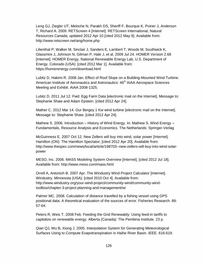
126

Leng GJ, Ziegler UT, Meloche N, Parakh DS, Sheriff F, Bourque K, Poirier J, Anderson

T, Richard A. 2009. RETScreen 4 [Internet]. RETScreen International, Natural

Resources Canada; updated 2012 Apr 10 [cited 2012 May 9]. Available from:

http://www.retscreen.net/ang/home.php

Lilienthal P, Walker M, Sinclair J, Sanders E, Lambert T, Woods M, Southwick K,

Glassmire J, Johnson N, Gilman P, Hale J, et al. 2009 Jul 24. HOMER Version 2.68

[Internet]. HOMER Energy, National Renewable Energy Lab, U.S. Department of

Energy. Colorado (USA): [cited 2012 Mar 1]. Available from:

https://homerenergy.com/download.html

Lubitz D, Hakimi R. 2008 Jan. Effect of Roof Slope on a Building-Mounted Wind Turbine.

American Institute of Aeronautics and Astronautics: 46th AIAA Aerospace Sciences

Meeting and Exhibit. AIAA 2008-1325.

Lubitz D. 2011 Jul 12. Fwd: Egg Farm Data [electronic mail on the Internet]. Message to:

Stephanie Shaw and Adam Epstein. [cited 2012 Apr 24].

Mather C. 2012 Mar 14. Our Bergey 1 Kw wind turbine [electronic mail on the Internet].

Message to: Stephanie Shaw. [cited 2012 Apr 24].

Mathew S. 2006. Introduction – History of Wind Energy. In: Mathew S. Wind Energy –

Fundamentals, Resource Analysis and Economics. The Netherlands: Springer-Verlag

McGuinness E. 2007 Oct 12. New Zellers will buy into wind, solar power [Internet].

Hamilton (ON): The Hamilton Spectator; [cited 2012 Apr 20]. Available from:

http://www.thespec.com/news/local/article/198703--new-zellers-will-buy-into-wind-solar-

power

MESO, Inc. 2006. MASS Modeling System Overview [Internet]. [cited 2012 Jul 18].

Available from: http://www.meso.com/mass.html

Orrell A, Antonich B. 2007 Apr. The Windustry Wind Project Calculator [Internet].

Windustry. Minnesota (USA); [cited 2010 Oct 4]. Available from:

http://www.windustry.org/your-wind-project/community-wind/community-wind-

toolbox/chapter-3-project-planning-and-management/wi

Palmer MC. 2008. Calculation of distance travelled by a fishing vessel using GPS

positional data: A theoretical evaluation of the sources of error. Fisheries Research. 89:

57-64.

Peters R, Weis T. 2008 Feb. Feeding the Grid Renewably: Using feed-in tariffs to

capitalize on renewable energy. Alberta (Canada): The Pembina Institute. 23 p.

Qian QJ, Wu B, Xiong J. 2005. Interpolation System for Generating Meteorological

Surfaces Using to Compute Evapotranspiration in Haihe River Basin. IEEE. 616-619.

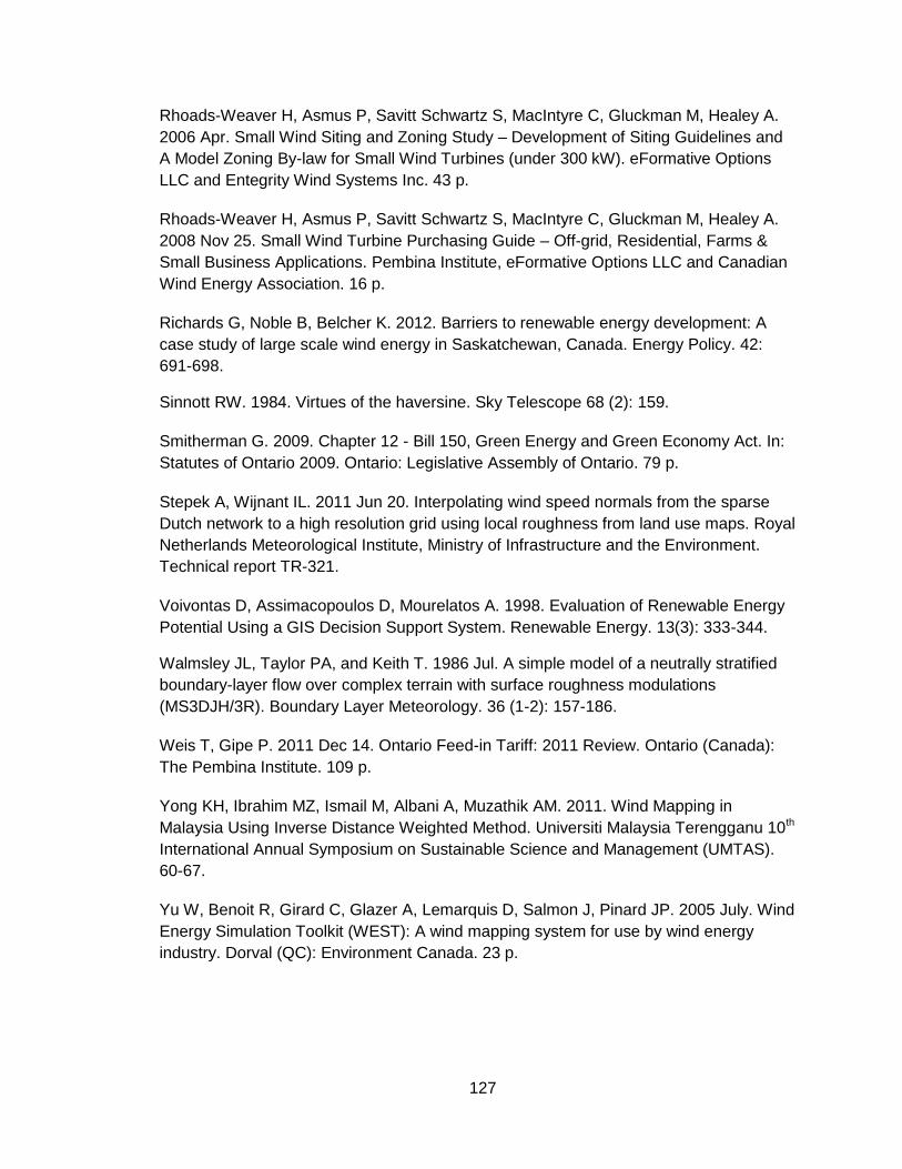
127

Rhoads-Weaver H, Asmus P, Savitt Schwartz S, MacIntyre C, Gluckman M, Healey A.

2006 Apr. Small Wind Siting and Zoning Study – Development of Siting Guidelines and

A Model Zoning By-law for Small Wind Turbines (under 300 kW). eFormative Options

LLC and Entegrity Wind Systems Inc. 43 p.

Rhoads-Weaver H, Asmus P, Savitt Schwartz S, MacIntyre C, Gluckman M, Healey A.

2008 Nov 25. Small Wind Turbine Purchasing Guide – Off-grid, Residential, Farms &

Small Business Applications. Pembina Institute, eFormative Options LLC and Canadian

Wind Energy Association. 16 p.

Richards G, Noble B, Belcher K. 2012. Barriers to renewable energy development: A

case study of large scale wind energy in Saskatchewan, Canada. Energy Policy. 42:

691-698.

Sinnott RW. 1984. Virtues of the haversine. Sky Telescope 68 (2): 159.

Smitherman G. 2009. Chapter 12 - Bill 150, Green Energy and Green Economy Act. In:

Statutes of Ontario 2009. Ontario: Legislative Assembly of Ontario. 79 p.

Stepek A, Wijnant IL. 2011 Jun 20. Interpolating wind speed normals from the sparse

Dutch network to a high resolution grid using local roughness from land use maps. Royal

Netherlands Meteorological Institute, Ministry of Infrastructure and the Environment.

Technical report TR-321.

Voivontas D, Assimacopoulos D, Mourelatos A. 1998. Evaluation of Renewable Energy

Potential Using a GIS Decision Support System. Renewable Energy. 13(3): 333-344.

Walmsley JL, Taylor PA, and Keith T. 1986 Jul. A simple model of a neutrally stratified

boundary-layer flow over complex terrain with surface roughness modulations

(MS3DJH/3R). Boundary Layer Meteorology. 36 (1-2): 157-186.

Weis T, Gipe P. 2011 Dec 14. Ontario Feed-in Tariff: 2011 Review. Ontario (Canada):

The Pembina Institute. 109 p.

Yong KH, Ibrahim MZ, Ismail M, Albani A, Muzathik AM. 2011. Wind Mapping in

Malaysia Using Inverse Distance Weighted Method. Universiti Malaysia Terengganu 10th

International Annual Symposium on Sustainable Science and Management (UMTAS).

60-67.

Yu W, Benoit R, Girard C, Glazer A, Lemarquis D, Salmon J, Pinard JP. 2005 July. Wind

Energy Simulation Toolkit (WEST): A wind mapping system for use by wind energy

industry. Dorval (QC): Environment Canada. 23 p.

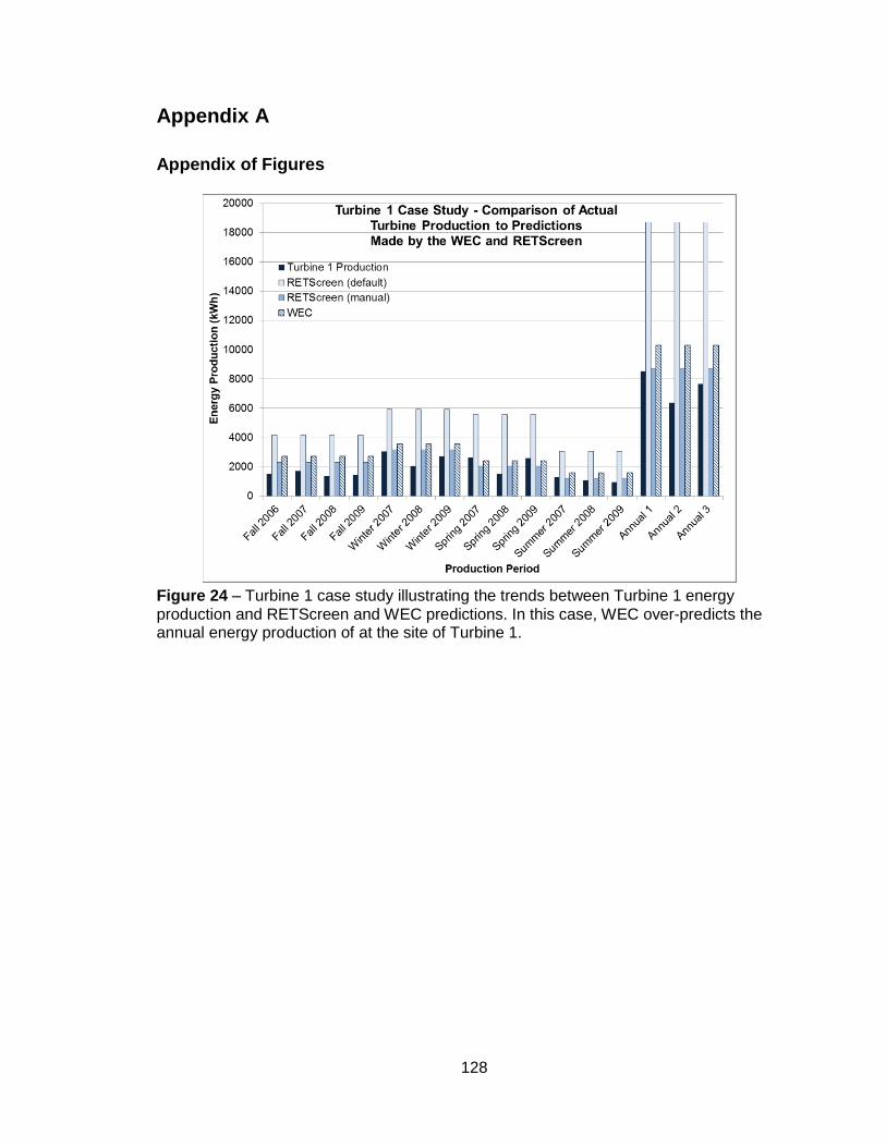
128

Appendix A

Appendix of Figures

Figure 24 – Turbine 1 case study illustrating the trends between Turbine 1 energy production and RETScreen and WEC predictions. In this case, WEC over-predicts the annual energy production of at the site of Turbine 1.

129

Figure 25 – Turbine 2 case study illustrating the trends between Turbine 2 energy production and RETScreen and WEC predictions for this site. In this case, WEC over-predicts the annual energy production of the turbine at site 2.

Figure 26 – Turbine 3 case study illustrating the trends between Turbine 3 energy production and RETScreen and WEC predictions for that site. In this case, the WEC and RETScreen (manual) are fairly close at predicting the annual energy production.

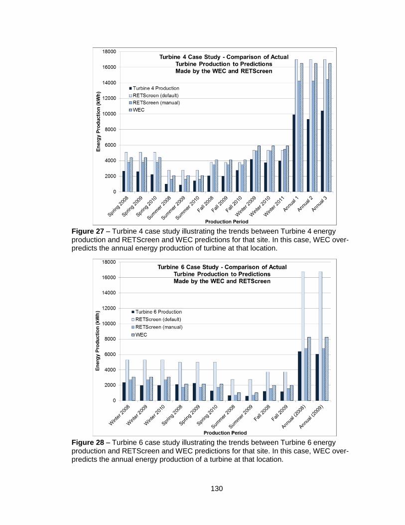
130

Figure 27 – Turbine 4 case study illustrating the trends between Turbine 4 energy production and RETScreen and WEC predictions for that site. In this case, WEC over-predicts the annual energy production of turbine at that location.

Figure 28 – Turbine 6 case study illustrating the trends between Turbine 6 energy production and RETScreen and WEC predictions for that site. In this case, WEC over-predicts the annual energy production of a turbine at that location.

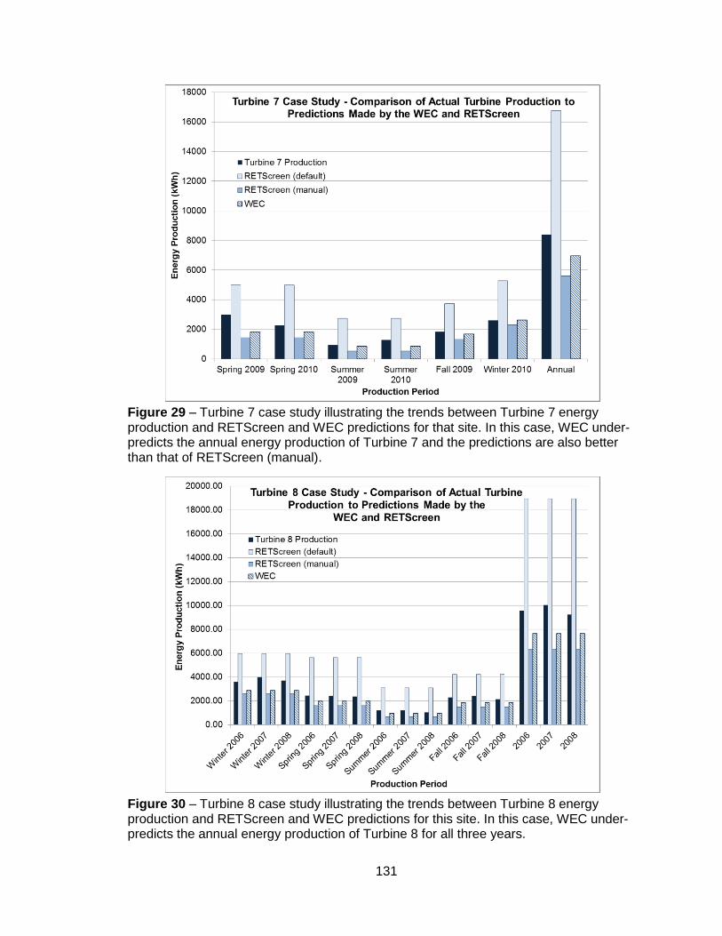
131

Figure 29 – Turbine 7 case study illustrating the trends between Turbine 7 energy production and RETScreen and WEC predictions for that site. In this case, WEC under-predicts the annual energy production of Turbine 7 and the predictions are also better than that of RETScreen (manual).

Figure 30 – Turbine 8 case study illustrating the trends between Turbine 8 energy production and RETScreen and WEC predictions for this site. In this case, WEC under-predicts the annual energy production of Turbine 8 for all three years.

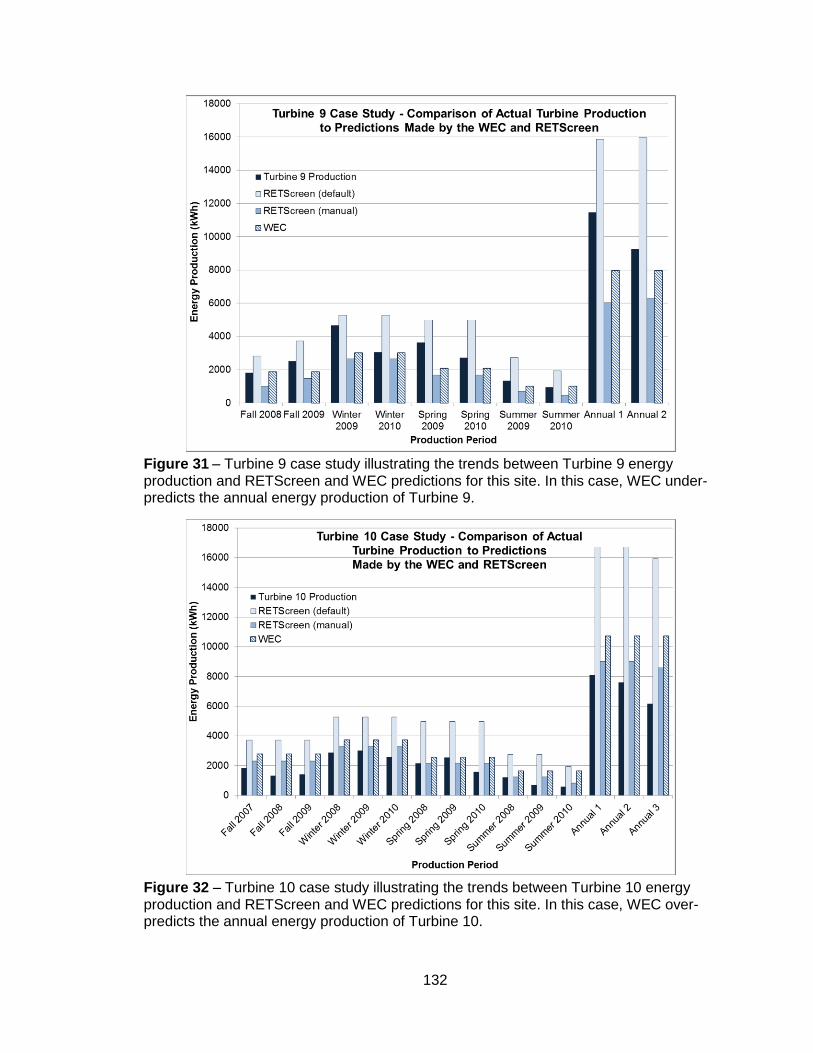
132

Figure 31 – Turbine 9 case study illustrating the trends between Turbine 9 energy production and RETScreen and WEC predictions for this site. In this case, WEC under-predicts the annual energy production of Turbine 9.

Figure 32 – Turbine 10 case study illustrating the trends between Turbine 10 energy production and RETScreen and WEC predictions for this site. In this case, WEC over-predicts the annual energy production of Turbine 10.

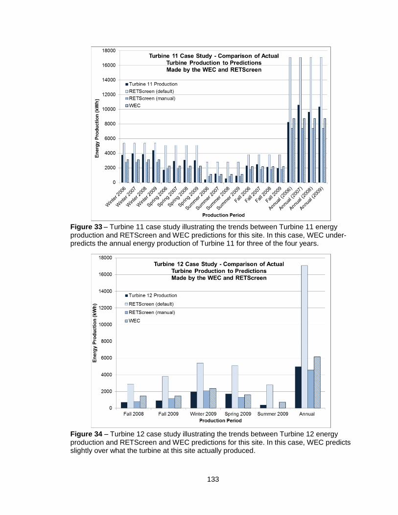
133

Figure 33 – Turbine 11 case study illustrating the trends between Turbine 11 energy production and RETScreen and WEC predictions for this site. In this case, WEC under-predicts the annual energy production of Turbine 11 for three of the four years.

Figure 34 – Turbine 12 case study illustrating the trends between Turbine 12 energy production and RETScreen and WEC predictions for this site. In this case, WEC predicts slightly over what the turbine at this site actually produced.

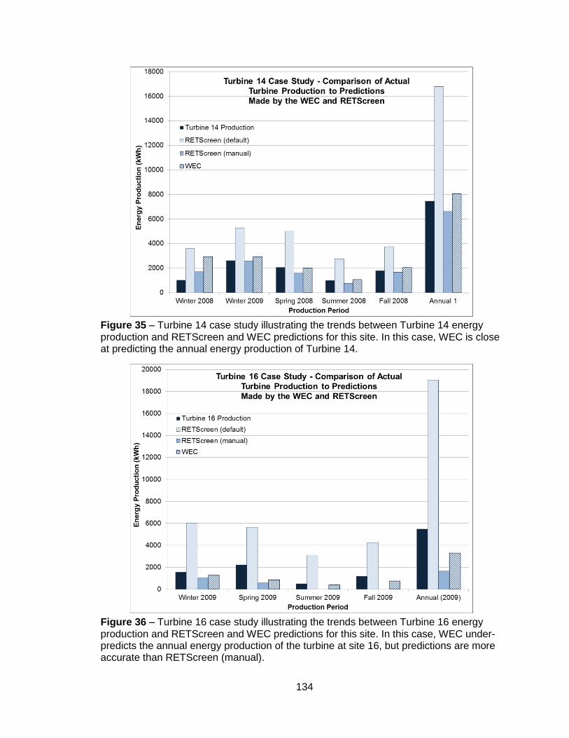
134

Figure 35 – Turbine 14 case study illustrating the trends between Turbine 14 energy production and RETScreen and WEC predictions for this site. In this case, WEC is close at predicting the annual energy production of Turbine 14.

Figure 36 – Turbine 16 case study illustrating the trends between Turbine 16 energy production and RETScreen and WEC predictions for this site. In this case, WEC under-predicts the annual energy production of the turbine at site 16, but predictions are more accurate than RETScreen (manual).

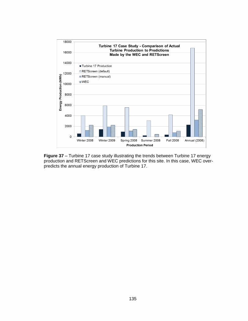
135

Figure 37 – Turbine 17 case study illustrating the trends between Turbine 17 energy production and RETScreen and WEC predictions for this site. In this case, WEC over-predicts the annual energy production of Turbine 17.

Appendix B

Appendix of Tables

Table 18 – Table with data comparing: the impact of p in the IDW method on WEC predictions, the ratio of actual production to WEC (p=1.5) predicted value, and the percent deviation between the WEC (p=1.5) prediction and actual turbine production.

Production Period

Turbine Production

(kWh)

WEC Prediction (kWh) Ratio =

% Deviation =

(

) p=1 p=1.5 p=2

Turbine 1

Fall 2006 1516.63 2605.97 2729.62 2493.00 0.56 80.0%

Fall 2007 1727.52 2605.97 2729.62 2493.00 0.63 58.0%

Fall 2008 1381.00 2605.97 2729.62 2493.00 0.51 97.7%

Fall 2009 1444.00 2605.97 2729.62 2493.00 0.53 89.0%

Winter 2007 3055.77 3484.18 3550.15 3363.57 0.86 16.2%

Winter 2008 2050.74 3484.18 3550.15 3363.57 0.58 73.1%

Winter 2009 2731.00 3484.18 3550.15 3363.57 0.77 30.0%

Spring 2007 2650.43 2329.98 2421.74 2227.49 1.09 -8.6%

Spring 2008 1519.26 2329.98 2421.74 2227.49 0.63 59.4%

Spring 2009 2581.00 2329.98 2421.74 2227.49 1.07 -6.2%

Summer 2007 1315.06 1510.25 1596.93 1434.92 0.82 21.4%

Summer 2008 1077.46 1510.25 1596.93 1434.92 0.67 48.2%

Summer 2009 960.00 1510.25 1596.93 1434.92 0.60 66.3%

Year 1 8537.88 9930.37 10298.43 9518.98 0.83 20.6%

Year 2 6374.98 9930.37 10298.43 9518.98 0.62 61.5%

Year 3 7653.00 9930.37 10298.43 9518.98 0.74 34.6%

136

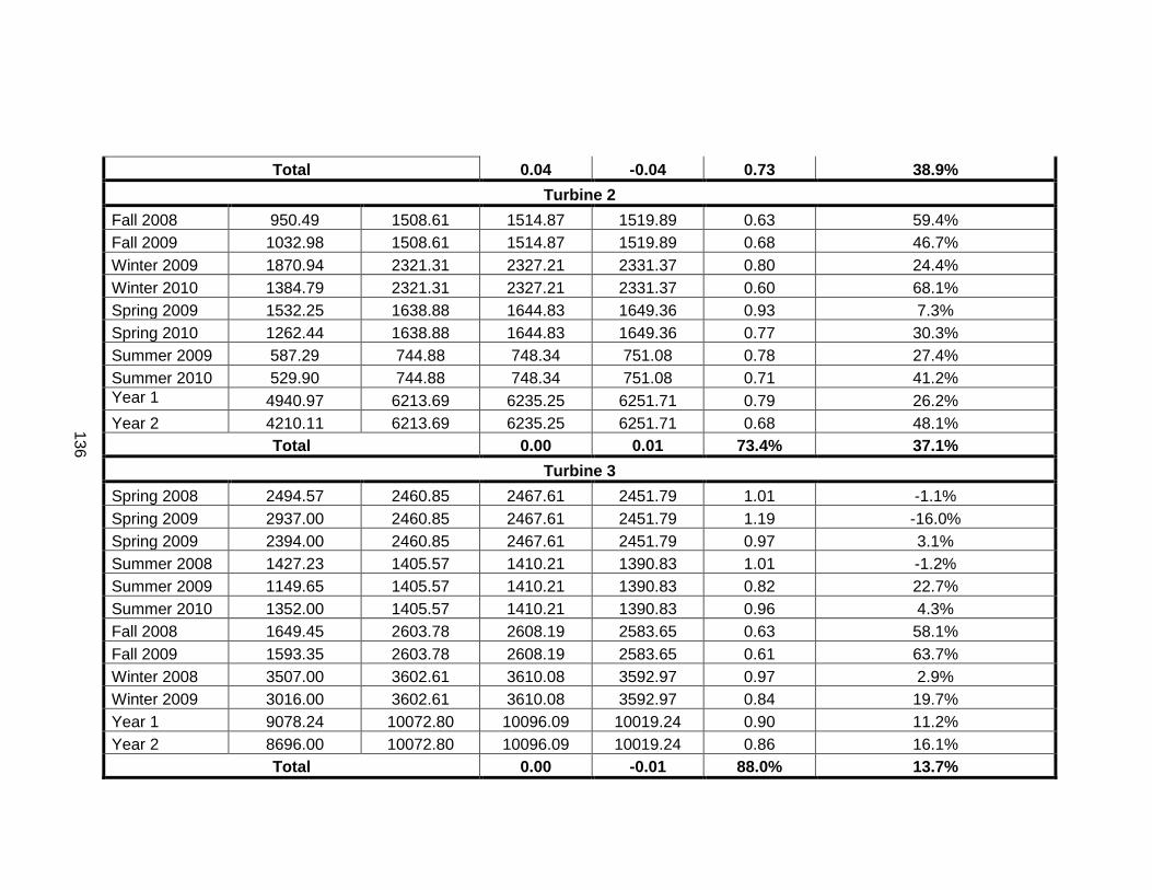
Total 0.04 -0.04 0.73 38.9%

Turbine 2

Fall 2008 950.49 1508.61 1514.87 1519.89 0.63 59.4%

Fall 2009 1032.98 1508.61 1514.87 1519.89 0.68 46.7%

Winter 2009 1870.94 2321.31 2327.21 2331.37 0.80 24.4%

Winter 2010 1384.79 2321.31 2327.21 2331.37 0.60 68.1%

Spring 2009 1532.25 1638.88 1644.83 1649.36 0.93 7.3%

Spring 2010 1262.44 1638.88 1644.83 1649.36 0.77 30.3%

Summer 2009 587.29 744.88 748.34 751.08 0.78 27.4%

Summer 2010 529.90 744.88 748.34 751.08 0.71 41.2%

Year 1 4940.97 6213.69 6235.25 6251.71 0.79 26.2%

Year 2 4210.11 6213.69 6235.25 6251.71 0.68 48.1%

Total 0.00 0.01 73.4% 37.1%

Turbine 3

Spring 2008 2494.57 2460.85 2467.61 2451.79 1.01 -1.1%

Spring 2009 2937.00 2460.85 2467.61 2451.79 1.19 -16.0%

Spring 2009 2394.00 2460.85 2467.61 2451.79 0.97 3.1%

Summer 2008 1427.23 1405.57 1410.21 1390.83 1.01 -1.2%

Summer 2009 1149.65 1405.57 1410.21 1390.83 0.82 22.7%

Summer 2010 1352.00 1405.57 1410.21 1390.83 0.96 4.3%

Fall 2008 1649.45 2603.78 2608.19 2583.65 0.63 58.1%

Fall 2009 1593.35 2603.78 2608.19 2583.65 0.61 63.7%

Winter 2008 3507.00 3602.61 3610.08 3592.97 0.97 2.9%

Winter 2009 3016.00 3602.61 3610.08 3592.97 0.84 19.7%

Year 1 9078.24 10072.80 10096.09 10019.24 0.90 11.2%

Year 2 8696.00 10072.80 10096.09 10019.24 0.86 16.1%

Total 0.00 -0.01 88.0% 13.7%

136

Turbine 4

Spring 2008 2671.06 4269.65 4408.15 4532.60 0.61 65.0%

Spring 2009 2630.00 4269.65 4408.15 4532.60 0.60 67.6%

Spring 2010 2240.52 4269.65 4408.15 4532.60 0.51 96.7%

Summer 2008 1002.06 2064.92 2090.06 2124.90 0.48 108.6%

Summer 2009 910.00 2064.92 2090.06 2124.90 0.44 129.7%

Summer 2010 1432.48 2064.92 2090.06 2124.90 0.69 45.9%

Fall 2008 2075.18 4012.16 4094.63 4179.95 0.51 97.3%

Fall 2009 2032.00 4012.16 4094.63 4179.95 0.50 101.5%

Fall 2010 2771.00 4012.16 4094.63 4179.95 0.68 47.8%

Winter 2009 4195.33 5750.96 5904.45 6043.95 0.71 40.7%

Winter 2010 3765.00 5750.96 5904.45 6043.95 0.64 56.8%

Winter 2011 3989.00 5750.96 5904.45 6043.95 0.68 48.0%

Year 1 9943.64 16097.69 16497.29 16881.40 0.60 65.9%

Year 2 9337.00 16097.69 16497.29 16881.40 0.57 76.7%

Year 3 10433.00 16097.69 16497.29 16881.40 0.63 58.1%

Total 0.02 0.05 60.0% 66.9%

Turbine 5

Summer 2009 1215.76 937.90 919.37 928.05 1.32 -24.4%

Fall 2009 2299.26 1803.22 1777.39 1787.54 1.29 -22.7%

Winter 2010 2873.44 2627.72 2594.40 2600.07 1.11 -9.7%

Spring 2010 2471.00 1840.74 1826.64 1828.84 1.35 -26.1%

Year 1 8859.47 7209.57 7117.80 7144.49 1.24 -19.7%

Total -0.01 -0.01 124.5% -19.7%

Turbine 6

Winter 2008 2392.00 3014.39 3086.54 3047.72 0.77 29.0%

Winter 2009 1994.10 3014.39 3086.54 3047.72 0.65 54.8%

138

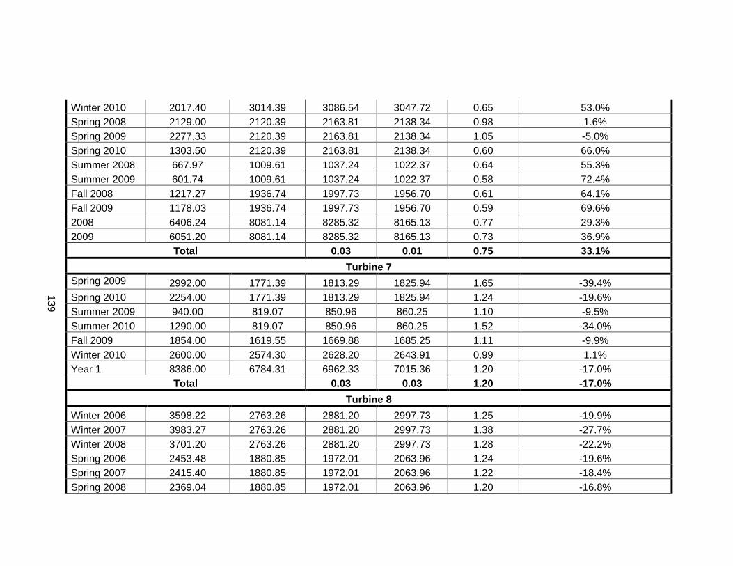
Winter 2010 2017.40 3014.39 3086.54 3047.72 0.65 53.0%

Spring 2008 2129.00 2120.39 2163.81 2138.34 0.98 1.6%

Spring 2009 2277.33 2120.39 2163.81 2138.34 1.05 -5.0%

Spring 2010 1303.50 2120.39 2163.81 2138.34 0.60 66.0%

Summer 2008 667.97 1009.61 1037.24 1022.37 0.64 55.3%

Summer 2009 601.74 1009.61 1037.24 1022.37 0.58 72.4%

Fall 2008 1217.27 1936.74 1997.73 1956.70 0.61 64.1%

Fall 2009 1178.03 1936.74 1997.73 1956.70 0.59 69.6%

2008 6406.24 8081.14 8285.32 8165.13 0.77 29.3%

2009 6051.20 8081.14 8285.32 8165.13 0.73 36.9%

Total 0.03 0.01 0.75 33.1%

Turbine 7

Spring 2009 2992.00 1771.39 1813.29 1825.94 1.65 -39.4%

Spring 2010 2254.00 1771.39 1813.29 1825.94 1.24 -19.6%

Summer 2009 940.00 819.07 850.96 860.25 1.10 -9.5%

Summer 2010 1290.00 819.07 850.96 860.25 1.52 -34.0%

Fall 2009 1854.00 1619.55 1669.88 1685.25 1.11 -9.9%

Winter 2010 2600.00 2574.30 2628.20 2643.91 0.99 1.1%

Year 1 8386.00 6784.31 6962.33 7015.36 1.20 -17.0%

Total 0.03 0.03 1.20 -17.0%

Turbine 8

Winter 2006 3598.22 2763.26 2881.20 2997.73 1.25 -19.9%

Winter 2007 3983.27 2763.26 2881.20 2997.73 1.38 -27.7%

Winter 2008 3701.20 2763.26 2881.20 2997.73 1.28 -22.2%

Spring 2006 2453.48 1880.85 1972.01 2063.96 1.24 -19.6%

Spring 2007 2415.40 1880.85 1972.01 2063.96 1.22 -18.4%

Spring 2008 2369.04 1880.85 1972.01 2063.96 1.20 -16.8%

13

9

Summer 2006 1214.60 894.92 945.93 997.28 1.28 -22.1%

Summer 2007 1217.21 894.92 945.93 997.28 1.29 -22.3%

Summer 2008 1027.26 894.92 945.93 997.28 1.09 -7.9%

Fall 2006 2283.53 1750.87 1846.50 1941.50 1.24 -19.1%

Fall 2007 2417.69 1750.87 1846.50 1941.50 1.31 -23.6%

Fall 2008 2148.71 1750.87 1846.50 1941.50 1.16 -14.1%

2006 9549.82 7289.90 7645.64 8000.47 1.25 -19.9%

2007 10033.57 7289.90 7645.64 8000.47 1.31 -23.8%

2008 9246.21 7289.90 7645.64 8000.47 1.21 -17.3%

Total 0.05 0.10 125.7% -20.3%

Turbine 9

Fall 2008 1813.00 1877.88 1869.82 1866.40 0.97 3.1%

Fall 2009 2521.00 1877.88 1869.82 1866.40 1.35 -25.8%

Winter 2009 4672.00 3031.19 3012.25 3001.41 1.55 -35.5%

Winter 2010 3055.00 3031.19 3012.25 3001.41 1.01 -1.4%

Spring 2009 3643.00 2086.82 2076.88 2072.78 1.75 -43.0%

Spring 2010 2729.00 2086.82 2076.88 2072.78 1.31 -23.9%

Summer 2009 1337.00 1006.29 996.29 992.08 1.34 -25.5%

Summer 2010 940.00 1006.29 996.29 992.08 0.94 6.0%

Year 1 11465.00 8002.16 7955.24 7932.68 1.44 -30.6%

Year 2 9245.00 8002.16 7955.24 7932.68 1.16 -14.0%

Total -0.01 -0.01 1.30 -22.3%

Turbine 10

Fall 2007 1837.41 2868.04 2778.88 2687.78 0.66 51.2%

Fall 2008 1334.21 2868.04 2778.88 2687.78 0.48 108.3%

Fall 2009 1411.13 2868.04 2778.88 2687.78 0.51 96.9%

Winter 2008 2871.24 3844.53 3736.74 3626.50 0.77 30.1%

140

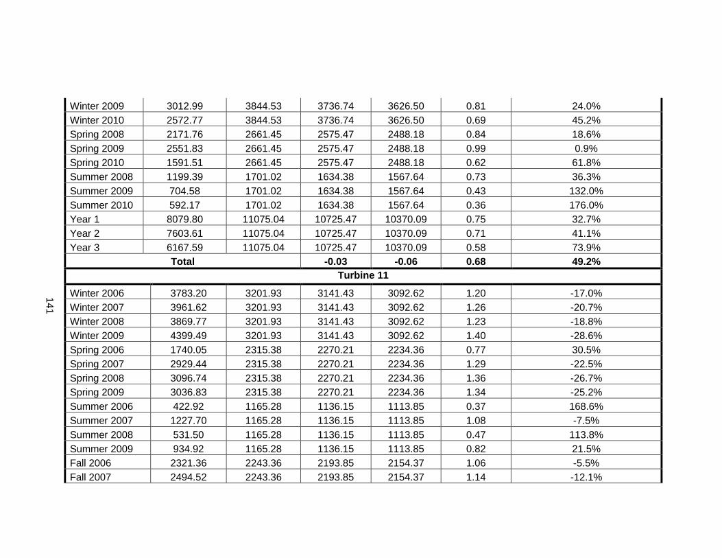
Winter 2009 3012.99 3844.53 3736.74 3626.50 0.81 24.0%

Winter 2010 2572.77 3844.53 3736.74 3626.50 0.69 45.2%

Spring 2008 2171.76 2661.45 2575.47 2488.18 0.84 18.6%

Spring 2009 2551.83 2661.45 2575.47 2488.18 0.99 0.9%

Spring 2010 1591.51 2661.45 2575.47 2488.18 0.62 61.8%

Summer 2008 1199.39 1701.02 1634.38 1567.64 0.73 36.3%

Summer 2009 704.58 1701.02 1634.38 1567.64 0.43 132.0%

Summer 2010 592.17 1701.02 1634.38 1567.64 0.36 176.0%

Year 1 8079.80 11075.04 10725.47 10370.09 0.75 32.7%

Year 2 7603.61 11075.04 10725.47 10370.09 0.71 41.1%

Year 3 6167.59 11075.04 10725.47 10370.09 0.58 73.9%

Total -0.03 -0.06 0.68 49.2%

Turbine 11

Winter 2006 3783.20 3201.93 3141.43 3092.62 1.20 -17.0%

Winter 2007 3961.62 3201.93 3141.43 3092.62 1.26 -20.7%

Winter 2008 3869.77 3201.93 3141.43 3092.62 1.23 -18.8%

Winter 2009 4399.49 3201.93 3141.43 3092.62 1.40 -28.6%

Spring 2006 1740.05 2315.38 2270.21 2234.36 0.77 30.5%

Spring 2007 2929.44 2315.38 2270.21 2234.36 1.29 -22.5%

Spring 2008 3096.74 2315.38 2270.21 2234.36 1.36 -26.7%

Spring 2009 3036.83 2315.38 2270.21 2234.36 1.34 -25.2%

Summer 2006 422.92 1165.28 1136.15 1113.85 0.37 168.6%

Summer 2007 1227.70 1165.28 1136.15 1113.85 1.08 -7.5%

Summer 2008 531.50 1165.28 1136.15 1113.85 0.47 113.8%

Summer 2009 934.92 1165.28 1136.15 1113.85 0.82 21.5%

Fall 2006 2321.36 2243.36 2193.85 2154.37 1.06 -5.5%

Fall 2007 2494.52 2243.36 2193.85 2154.37 1.14 -12.1%

14

1

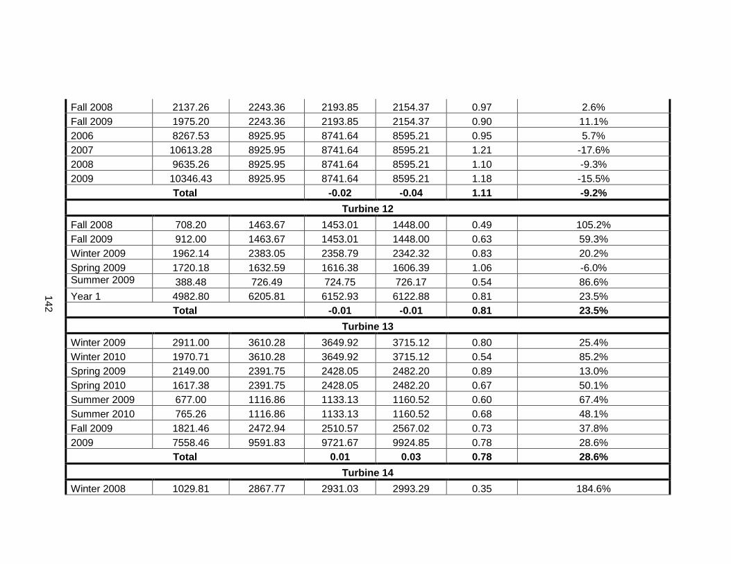
Fall 2008 2137.26 2243.36 2193.85 2154.37 0.97 2.6%

Fall 2009 1975.20 2243.36 2193.85 2154.37 0.90 11.1%

2006 8267.53 8925.95 8741.64 8595.21 0.95 5.7%

2007 10613.28 8925.95 8741.64 8595.21 1.21 -17.6%

2008 9635.26 8925.95 8741.64 8595.21 1.10 -9.3%

2009 10346.43 8925.95 8741.64 8595.21 1.18 -15.5%

Total -0.02 -0.04 1.11 -9.2%

Turbine 12

Fall 2008 708.20 1463.67 1453.01 1448.00 0.49 105.2%

Fall 2009 912.00 1463.67 1453.01 1448.00 0.63 59.3%

Winter 2009 1962.14 2383.05 2358.79 2342.32 0.83 20.2%

Spring 2009 1720.18 1632.59 1616.38 1606.39 1.06 -6.0%

Summer 2009 388.48 726.49 724.75 726.17 0.54 86.6%

Year 1 4982.80 6205.81 6152.93 6122.88 0.81 23.5%

Total -0.01 -0.01 0.81 23.5%

Turbine 13

Winter 2009 2911.00 3610.28 3649.92 3715.12 0.80 25.4%

Winter 2010 1970.71 3610.28 3649.92 3715.12 0.54 85.2%

Spring 2009 2149.00 2391.75 2428.05 2482.20 0.89 13.0%

Spring 2010 1617.38 2391.75 2428.05 2482.20 0.67 50.1%

Summer 2009 677.00 1116.86 1133.13 1160.52 0.60 67.4%

Summer 2010 765.26 1116.86 1133.13 1160.52 0.68 48.1%

Fall 2009 1821.46 2472.94 2510.57 2567.02 0.73 37.8%

2009 7558.46 9591.83 9721.67 9924.85 0.78 28.6%

Total 0.01 0.03 0.78 28.6%

Turbine 14

Winter 2008 1029.81 2867.77 2931.03 2993.29 0.35 184.6%

14

2

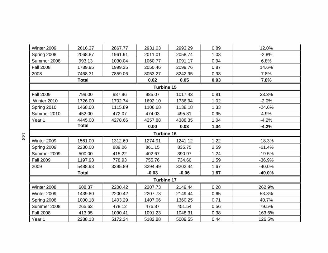
Winter 2009 2616.37 2867.77 2931.03 2993.29 0.89 12.0%

Spring 2008 2068.87 1961.91 2011.01 2058.74 1.03 -2.8%

Summer 2008 993.13 1030.04 1060.77 1091.17 0.94 6.8%

Fall 2008 1789.95 1999.35 2050.46 2099.76 0.87 14.6%

2008 7468.31 7859.06 8053.27 8242.95 0.93 7.8%

Total 0.02 0.05 0.93 7.8%

Turbine 15

Fall 2009 799.00 987.96 985.07 1017.43 0.81 23.3%

Winter 2010 1726.00 1702.74 1692.10 1736.94 1.02 -2.0%

Spring 2010 1468.00 1115.89 1106.68 1138.18 1.33 -24.6%

Summer 2010 452.00 472.07 474.03 495.81 0.95 4.9%

Year 1 4445.00 4278.66 4257.88 4388.35 1.04 -4.2%

Total 0.00 0.03 1.04 -4.2%

Turbine 16

Winter 2009 1561.00 1312.69 1274.91 1241.12 1.22 -18.3%

Spring 2009 2230.00 889.06 861.15 835.75 2.59 -61.4%

Summer 2009 500.00 415.22 402.67 390.97 1.24 -19.5%

Fall 2009 1197.93 778.93 755.76 734.60 1.59 -36.9%

2009 5488.93 3395.89 3294.49 3202.44 1.67 -40.0%

Total -0.03 -0.06 1.67 -40.0%

Turbine 17

Winter 2008 608.37 2200.42 2207.73 2149.44 0.28 262.9%

Winter 2009 1439.80 2200.42 2207.73 2149.44 0.65 53.3%

Spring 2008 1000.18 1403.29 1407.06 1360.25 0.71 40.7%

Summer 2008 265.63 478.12 476.87 451.54 0.56 79.5%

Fall 2008 413.95 1090.41 1091.23 1048.31 0.38 163.6%

Year 1 2288.13 5172.24 5182.88 5009.55 0.44 126.5%

14

3

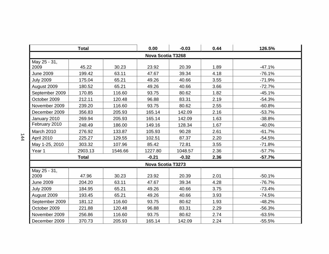
Total 0.00 -0.03 0.44 126.5%

Nova Scotia T3268

May 25 - 31, 2009 45.22 30.23 23.92 20.39 1.89 -47.1%

June 2009 199.42 63.11 47.67 39.34 4.18 -76.1%

July 2009 175.04 65.21 49.26 40.66 3.55 -71.9%

August 2009 180.52 65.21 49.26 40.66 3.66 -72.7%

September 2009 170.85 116.60 93.75 80.62 1.82 -45.1%

October 2009 212.11 120.48 96.88 83.31 2.19 -54.3%

November 2009 239.20 116.60 93.75 80.62 2.55 -60.8%

December 2009 356.83 205.93 165.14 142.09 2.16 -53.7%

January 2010 269.94 205.93 165.14 142.09 1.63 -38.8%

February 2010 248.49 186.00 149.16 128.34 1.67 -40.0%

March 2010 276.92 133.87 105.93 90.28 2.61 -61.7%

April 2010 225.27 129.55 102.51 87.37 2.20 -54.5%

May 1-25, 2010 303.32 107.96 85.42 72.81 3.55 -71.8%

Year 1 2903.13 1546.66 1227.80 1048.57 2.36 -57.7%

Total -0.21 -0.32 2.36 -57.7%

Nova Scotia T3273

May 25 - 31, 2009 47.96 30.23 23.92 20.39 2.01 -50.1%

June 2009 204.20 63.11 47.67 39.34 4.28 -76.7%

July 2009 184.95 65.21 49.26 40.66 3.75 -73.4%

August 2009 193.45 65.21 49.26 40.66 3.93 -74.5%

September 2009 181.12 116.60 93.75 80.62 1.93 -48.2%

October 2009 221.88 120.48 96.88 83.31 2.29 -56.3%

November 2009 256.86 116.60 93.75 80.62 2.74 -63.5%

December 2009 370.73 205.93 165.14 142.09 2.24 -55.5%

14

4

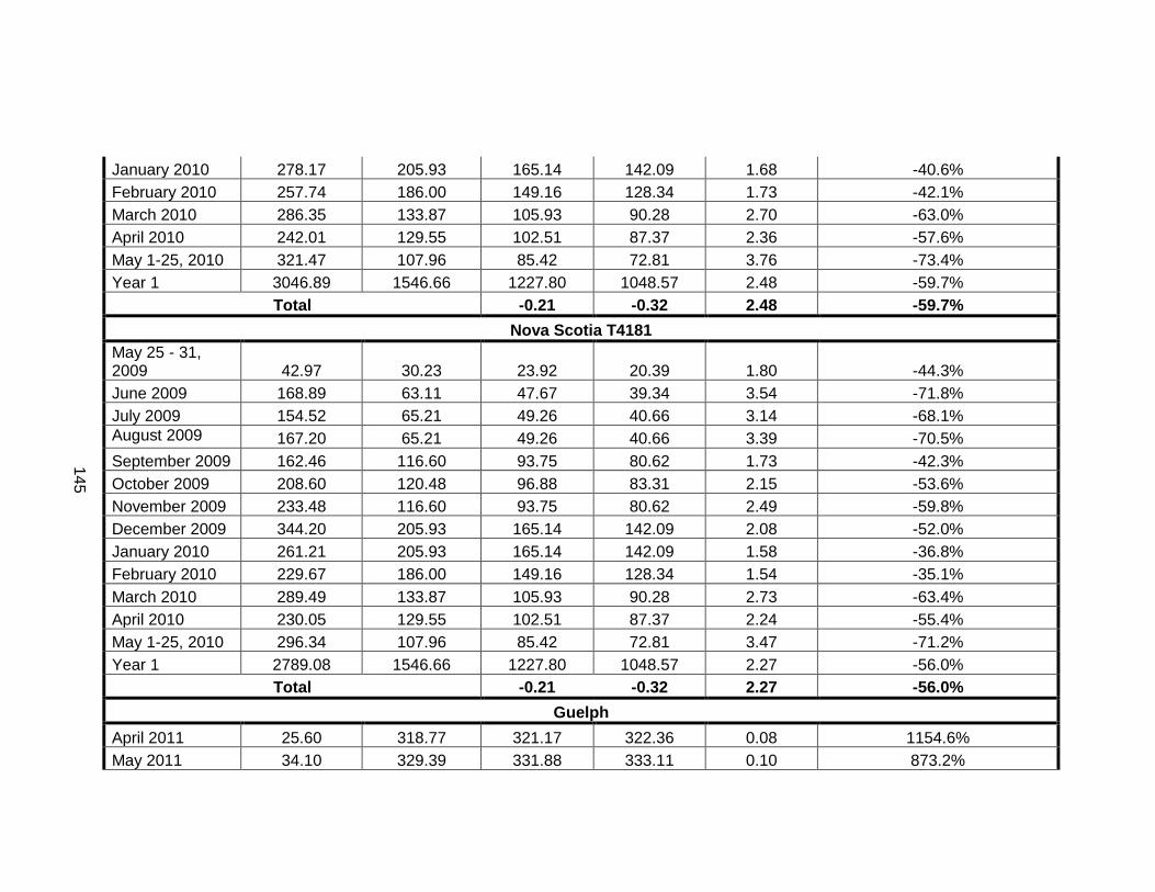
January 2010 278.17 205.93 165.14 142.09 1.68 -40.6%

February 2010 257.74 186.00 149.16 128.34 1.73 -42.1%

March 2010 286.35 133.87 105.93 90.28 2.70 -63.0%

April 2010 242.01 129.55 102.51 87.37 2.36 -57.6%

May 1-25, 2010 321.47 107.96 85.42 72.81 3.76 -73.4%

Year 1 3046.89 1546.66 1227.80 1048.57 2.48 -59.7%

Total -0.21 -0.32 2.48 -59.7%

Nova Scotia T4181

May 25 - 31, 2009 42.97 30.23 23.92 20.39 1.80 -44.3%

June 2009 168.89 63.11 47.67 39.34 3.54 -71.8%

July 2009 154.52 65.21 49.26 40.66 3.14 -68.1%

August 2009 167.20 65.21 49.26 40.66 3.39 -70.5%

September 2009 162.46 116.60 93.75 80.62 1.73 -42.3%

October 2009 208.60 120.48 96.88 83.31 2.15 -53.6%

November 2009 233.48 116.60 93.75 80.62 2.49 -59.8%

December 2009 344.20 205.93 165.14 142.09 2.08 -52.0%

January 2010 261.21 205.93 165.14 142.09 1.58 -36.8%

February 2010 229.67 186.00 149.16 128.34 1.54 -35.1%

March 2010 289.49 133.87 105.93 90.28 2.73 -63.4%

April 2010 230.05 129.55 102.51 87.37 2.24 -55.4%

May 1-25, 2010 296.34 107.96 85.42 72.81 3.47 -71.2%

Year 1 2789.08 1546.66 1227.80 1048.57 2.27 -56.0%

Total -0.21 -0.32 2.27 -56.0%

Guelph

April 2011 25.60 318.77 321.17 322.36 0.08 1154.6%

May 2011 34.10 329.39 331.88 333.11 0.10 873.2%

14

5

June 2011 27.30 147.52 148.06 148.48 0.18 442.4%

July 2011 20.70 152.44 153.00 153.43 0.14 639.1%

August 2011 19.50 152.44 153.00 153.43 0.13 684.6%

September 2011 16.80 341.27 343.71 344.66 0.05 1945.9%

October 2011 35.50 352.65 355.17 356.15 0.10 900.5%

November 2011 51.50 341.27 343.71 344.66 0.15 567.4%

December 2011 40.00 541.67 545.27 547.20 0.07 1263.2%

January 2012 53.70 541.67 545.27 547.20 0.10 915.4%

February 2012 45.90 489.25 492.50 494.24 0.09 973.0%

March 2012 37.90 329.39 331.88 333.11 0.11 775.7%

Year 1 271.00 2677.43 2694.97 2703.50 0.10 894.5%

Total 0.01 0.01 0.11 925.3%

146

Development and Validation of the Wind Energy Calculator (WEC

Documents

Transcript of Development and Validation of the Wind Energy Calculator (WEC