Development and Testing of Augmentations of Continuously ... · i Continuously -operating networks...

Development and Testing of Augmentations

of Continuously-Operating GPS Networks

to Improve Their Spatial and Temporal Resolution

By

Linlin Ge

M.Sc., Institute of Seismology, State Seismological Bureau, P.R. China, 1988.

B.Eng. (1st Hons), Wuhan Technical University of Surveying and Mapping, P.R. China,

1985.

A thesis submitted to The University of New South Wales

in partial fulfillment of the requirements for the degree of

Doctor of Philosophy

School of Geomatic Engineering

The University of New South Wales

Sydney NSW 2052, Australia

November 2000

i

Continuously-operating networks of GPS receivers (CGPS) are not capable of determining

the characteristics of crustal deformation at the fine temporal or spatial scales required.

Four ‘temporal densification schemes’ and two 'spatial densification schemes' to augment

the CGPS networks have been developed and tested.

The four ‘temporal densification schemes’ are based on the high rate Real-Time Kinematic

(RTK) GPS technique, GPS multipath effects, Very Long Baseline Interferometry (VLBI)

and Satellite Laser Ranging (SLR).

The 'serial scheme' based on using GPS as a seismometer has been proposed. Simulated

seismic signals have been extracted from the very noisy high rate RTK-GPS results using

an adaptive filter based on the least-mean-square algorithm. They are in very good

agreement with those of the collocated seismometers. This scheme can improve the CGPS

temporal resolution to 0.1 second.

The 'retro-active scheme' takes advantage of the fact that the GPS multipath disturbance is

repeated between consecutive days. It can therefore provide a means of correcting

multipath errors in the observation data themselves. A reduction of the standard deviations

of the pseudo-range and carrier phase multipath time series to about one fourth and one half

the original values respectively, has been demonstrated.

The 'all-GPS parallel scheme' uses the multipath effects as a signal to monitor the antenna

environment. Models relating the changes of multipath and antenna environment have been

derived.

The 'cross-technique parallel scheme' integrates the collocated CGPS, VLBI and SLR

results, taking advantage of the decorrelation among their biases and errors. Crustal

ABSTRACT

ii

displacement signature has been extracted as a common-mode signal using data from two

stations: Matera in Italy and Wettzell in Germany.

Two 'spatial densification schemes' which can verify with each other have been developed

and tested. The 'soft' scheme integrates CGPS with radar interferometry (InSAR). The

Double Interpolation and Double Prediction (DIDP) approach combines the strengths of the

high temporal resolution of CGPS and the high spatial resolution possible with the InSAR

technique. This scheme can improve the spatial resolution to about 25m.

The 'hard' scheme requires the deployment of single-frequency receivers to in-fill the

present CGPS arrays. Alternatively some receivers may be installed at some geophysically

strategic sites outside existing CGPS arrays. The former has been tested within Japan's

GEONET, while the latter has been tested using a five-station array.

iii

ABSTRACT................................................................................................................................ I

TABLE OF CONTENTS.......................................................................................................III

LIST OF FIGURES.............................................................................................................. VII

LIST OF TABLES.................................................................................................................XII

ACKNOWLEDGEMENTS ............................................................................................... XIV

1 INTRODUCTION ..............................................................................................................1

1.1 THE GLOBAL POSITIONING SYSTEM (GPS) ...................................................................1

1.2 THE NAVSTAR GPS MODERNIZATION .......................................................................4

1.3 CONTINUOUSLY-OPERATING NETWORKS OF GPS RECEIVERS (CGPS) .......................7

1.4 CGPS ACHIEVEMENTS...................................................................................................8

1.5 TEMPORAL AND SPATIAL RESOLUTION REQUIREMENTS ON CGPS FROM SOME

GEODYNAMIC AND ENGINEERING APPLICATIONS .................................................................10

1.6 METHODOLOGY ............................................................................................................13

1.7 CONTRIBUTIONS OF THE RESEARCH ............................................................................18

2 ADAPTIVE FILTER AND ASSOCIATED SIMULATION STUDIES..................20

2.1 THE ADAPTIVE FILTER .................................................................................................21

2.2 THE FILTER DESIGN......................................................................................................22

2.3 THE ADAPTIVE ALGORITHM DESIGN ...........................................................................24

2.4 THE REAL-TIME IMPLEMENTATION OF THE ADAPTIVE FILTER...................................26

2.5 EVALUATION OF THE LMS ALGORITHM .....................................................................29

2.6 IMPLEMENTING ISSUES OF THE ADAPTIVE FILTER ......................................................30

2.7 ADAPTIVE FILTERING OF SIMULATED DATA ...............................................................31

TABLE OF CONTENTS

iv

3 SERIAL TEMPORAL DENSIFICATION – THE 'GPS SEISMOMETER' .........37

3.1 GPS REAL-TIME KINEMATIC (RTK) APPLICATIONS..................................................37

3.1.1 Standard RTK .......................................................................................................37

3.1.2 Network RTK (the Virtual Reference Station concept) .....................................38

3.2 GPS SEISMOMETER – AN OVERVIEW ..........................................................................40

3.3 GPS SEISMOMETER – THE UNSW EXPERIMENT ........................................................42

3.3.1 The UNSW GPS Seismometer Experiment........................................................42

3.3.2 Fast RTK results ...................................................................................................44

3.3.3 Adaptive filtering of fast RTK results .................................................................52

3.3.4 Concluding remarks..............................................................................................58

3.4 GPS SEISMOMETER – THE UNSW-MRI EXPERIMENT ...............................................59

3.4.1 The UNSW-MRI GPS seismometer experiment ................................................59

3.4.2 Results and comparison........................................................................................62


3.5 GPS SEISMOMETER – THE IMPLEMENTING ISSUES .....................................................64

3.5.1 The layout of reference and rover receivers........................................................65

3.5.2 Noise reduction using measurements from adjacent days .................................68

3.5.3 Correlation between measurements.....................................................................72

3.5.4 Data communication.............................................................................................75

3.5.5 The Pros and Cons of using GPS as a seismometer ...........................................76


4 RETRO-ACTIVE TEMPORAL DENSIFICATION – MULTIPATH

MITIGATION..........................................................................................................................81

4.1 MULTIPATH MITIGATION – AN OVERVIEW .................................................................82

4.2 MULTIPATH COMBINATION ..............................................................................................84

4.3 PSEUDO-RANGE MULTIPATH MITIGATION USING THE ADAPTIVE FILTER ....................88

4.4 CARRIER-PHASE MULTIPATH MITIGATION USING THE ADAPTIVE FILTER....................93

4.5 MULTIPATH MITIGATION USING ADAPTIVE FILTERING APPLIED TO CGPS DATA.......95

4.6 IMPLEMENTING PROCEDURES FOR RETRO-ACTIVE TEMPORAL DENSIFICATION...........97

4.7 CONCLUDING REMARKS ...................................................................................................98

v

5 ALL-GPS PARALLEL TEMPORAL DENSIFICATION – THE USE OF

MULTIPATH EFFECTS AS A SIGNAL......................................................................... 100

5.1 INTRODUCTION .......................................................................................................... 101

5.2 MULTIPATH EXTRACTION ......................................................................................... 101

5.3 MULTIPATH CHANGE DETECTION............................................................................. 104

5.4 MULTIPATH CHANGE DETECTION IN A STATIONARY ANTENNA ENVIRONMENT.... 106

5.5 MULTIPATH CHANGE DETECTION IN A CHANGED ANTENNA ENVIRONMENT......... 114

5.6 SLOPE STABILITY MONITORING USING MULTIPATH CHANGE ................................ 119

5.6.1 Models for relating multipath to slope movement........................................... 120

5.6.2 The movement of slope and the change of geometric path length difference

between the direct and reflected signals......................................................................... 124

5.6.3 The change of multipath and the movement of slope...................................... 126

5.6.4 Least square estimation of slope movement using the change of multipath.. 130

5.7 CONCLUDING REMARKS............................................................................................ 131

6 CROSS-TECHNIQUE PARALLEL TEMPORAL DENSIFICATION – THE

INTEGRATION OF GPS WITH VLBI AND SLR ........................................................ 133

6.1 INTRODUCTION .......................................................................................................... 133

6.2 ANALYSES AND COMPARISONS OF THE BIASES AND ERRORS IN THE GPS, VLBI

AND SLR RESULTS.............................................................................................................. 135

6.3 THE INTEGRATION OF COLLOCATED GPS, VLBI AND SLR RESULTS ................... 141


7 SOFT SPATIAL DENSIFICATION – THE INTEGRATION OF GPS WITH

RADAR INTERFEROMETRY (INSAR) ........................................................................ 150

7.1 REVIEW OF RADAR INTERFEROMETRY (INSAR)...................................................... 150

7.1.1 Environment of InSAR studies ......................................................................... 154

7.1.2 InSAR for DEM................................................................................................. 156

7.1.3 InSAR for deformation (elevation change)...................................................... 159

7.1.4 Other InSAR applications ................................................................................. 160

7.2 COMPARISON BETWEEN CGPS AND INSAR............................................................ 161

vi

7.3 GPS AND INSAR INTEGRATION – THE "DOUBLE INTERPOLATION AND DOUBLE

PREDICTION" (DIDP) APPROACH ....................................................................................... 163

7.3.1 Deriving atmospheric correction to InSAR from CGPS................................. 164

7.3.2 Remove or mitigate SAR satellite orbit errors by using GPS results as

constraints ........................................................................................................................ 167

7.3.3 Densify observations by double interpolation ................................................. 169

7.3.4 Extrapolate quasi-observations by double prediction...................................... 179


8 HARD SPATIAL DENSIFICATION – INTEGRATING SINGLE- AND DUAL-

FREQUENCY GPS RECEIVERS..................................................................................... 181

8.1 COMPARISON BETWEEN SINGLE- AND DUAL-FREQUENCY GPS RECEIVERS......... 183

8.2 INWARD HARD SPATIAL DENSIFICATION – INTEGRATING SINGLE- AND DUAL-

FREQUENCY GPS RECEIVERS.............................................................................................. 186

8.3 THE UNSW-GSI HARD SPATIAL DENSIFICATION EXPERIMENT............................. 189

8.4 OUTWARD HARD SPATIAL DENSIFICATION - SEPARATING TECTONIC AND FAULT

MOVEMENTS FROM COMBINATIONS OF BASELINE SOLUTIONS ......................................... 194


9 SUMMARY, CONCLUSIONS AND RECOMMENDATIONS............................ 203

9.1 SUMMARY AND CONCLUSIONS.................................................................................. 203

9.1.1 Serial temporal densification – GPS seismometer........................................... 204

9.1.2 Retro-active temporal densification – multipath mitigation ........................... 208

9.1.3 All-GPS parallel temporal densification – the use of multipath effects as a

signal ............................................................................................................................. 208

9.1.4 Cross-technique parallel temporal densification – the integration of GPS with

VLBI and SLR................................................................................................................. 210

9.1.5 Soft spatial densification – the integration of GPS with radar interferometry

(INSAR) ........................................................................................................................... 210

9.1.6 Hard spatial densification.................................................................................. 211

9.2 RECOMMENDATIONS FOR FUTURE RESEARCH ......................................................... 212

REFERENCES ..................................................................................................................... 214

vii

Figure 1.1 The 24 NAVSTAR GPS satellites ...........................................................................3

Figure 1.2 GPS Modernization. ..................................................................................................5

Figure 1.3 Current and Proposed GPS Signal Spectrum...........................................................6

Figure 1.4 Future GPS Signal Structure.....................................................................................6

Figure 1.5 The first CGPS network............................................................................................8

Figure 1.6 The GEONET operated by the Geographical Survey Institute of Japan. ............10

Figure 1.7 Resolution requirements of some geophysical and geological applications . .....12

Figure 1.8 Temporal densification schemes. ...........................................................................14

Figure 1.9 Spatial densification schemes. ................................................................................16

Figure 2.1 The FIR filter scheme..............................................................................................24

Figure 2.2 Adaptive filtering configuration. ............................................................................32

Figure 2.3 Numerical simulation result of adaptive filtering of uncorrelated signals...........35

Figure 2.4 Numerical simulation result of adaptive filtering of partially correlated signals.

..............................................................................................................................................36

Figure 3.1 Setup of the UNSW GPS Seismometer Experiment.............................................43

Figure 3.2 System configuration for the GPS Seismometer Experiment...............................44

Figure 3.3 Comparison of fast RTK time series when the standard antenna is stationary and

vibrating . ............................................................................................................................45

Figure 3.4 Fast RTK time series using choke-ring antenna....................................................46

Figure 3.5 Frequency spectrum comparison, shaker vertical, 0Hz-2.3Hz-4.3Hz, standard

antenna.................................................................................................................................47

Figure 3.6 Frequency spectrum from the co-located accelerometer, 2.3Hz session. ............48

Figure 3.7 Frequency spectrum, 3 components, shaker 45 degree inclined, vibration 2.3Hz,

standard antenna. ................................................................................................................49

Figure 3.8 Frequency spectrum, 3 components, shaker vertical, vibration 2.3Hz, choke-ring

antenna.................................................................................................................................50

LIST OF FIGURES

viii

Figure 3.9 Frequency spectrum for height component, shaker vertical, 0Hz-2.3Hz-4.3Hz,

choke-ring antenna. ............................................................................................................51

Figure 3.10 Frequency spectrum for height component, comparison of 4.3Hz results for the

standard and choke-ring antennas......................................................................................51

Figure 3.11 Adaptive filtering configuration using the GPS-only approach. ........................53

Figure 3.12 Adaptive filtering result using the GPS-only approach. .....................................54

Figure 3.13 Adaptive filtering configuration using the GPS and accelerometer approach. .55

Figure 3.14 Adaptive filtering result using the GPS and accelerometer approach. ..............56

Figure 3.15 Adaptive filtering configuration using the Multi-template approach. ...............57

Figure 3.16 Adaptive filtering result using the multipath-template approach.......................58

Figure 3.17 Setup of the UNSW-MRI GPS Seismometer Experiment..................................60

Figure 3.18 Earthquake shake-simulator truck used in the UNSW-MRI GPS Seismometer

experiment...........................................................................................................................60

Figure 3.19 GPS RTK result compared with acceleration integrated twice and velocity

integrated once. ...................................................................................................................63

Figure 3.20 GPS RTK, acceleration and velocity after bandpass filtering. ...........................64

Figure 3.21 Configuration of reference and rover receivers in GPS seismometer system ..67

Figure 3.22 Moving baseline and DGPS positioning..............................................................68

Figure 3.23 Latitude variations of the rover RTK series on 5 successive days.....................69

Figure 3.24 Adaptive filtering used in noise reduction...........................................................70

Figure 3.25 Correlation analysis for L1 carrier phase ............................................................73

Figure 3.26 Correlation analysis for L2 carrier phase.............................................................73

Figure 3.27 Correlation analysis for P1 pseudo-range............................................................74

Figure 3.28 Correlation analysis for P2 pseudo-range............................................................74

Figure 4.1 Forward adaptive filtering results for pseudo-range multipath for the Day 1 and

Day 2 pair. ...........................................................................................................................88


Day 3 pair. ...........................................................................................................................89


Day 4 pair. ...........................................................................................................................90

ix


Day 3 pair. ...........................................................................................................................90


Day 4 pair. ...........................................................................................................................91

Figure 4.6 Backward adaptive filtering results for pseudo-range multipath for the Day 4 and

Day 1 pair. ...........................................................................................................................92

Figure 4.7 Forward adaptive filtering results for carrier phase multipath for the Day 1 and

Day 2 pair. ...........................................................................................................................94

Figure 4.8 Pseudo-range multipath for station BRAN of SCIGN .........................................96


Day 3 pair. ...........................................................................................................................96

Figure 5.1 Multipath change detection procedures. ............................................................. 105

Figure 5.2 Pseudo-range Multipath Combination Results. .................................................. 107

Figure 5.3 Multipath Extraction Result................................................................................. 108

Figure 5.4 Multipath Change Detection Result (Day 2-3)................................................... 109


Figure 5.6 Carrier phase multipath combination result........................................................ 111

Figure 5.7 Multipath Extraction Result................................................................................. 112



Figure 5.10 Precipitation and temperature in Tsukuba from 5 March (DOY 64) to 6 March

(DOY 65) 1998. ............................................................................................................... 115

Figure 5.11 Pseudo-range multipath change on C1 code at Station 960627 for satellite

PRN25. ............................................................................................................................. 116

Figure 5.12 Pseudo-range multipath change on C1 code at Station 92110 for satellite PRN

22. ..................................................................................................................................... 117

Figure 5.13 Carrier phase multipath change on L1 in DD between Stations 92110 and

960627 for satellite pair PRNs 22 and 25. ..................................................................... 118


960627 for satellite pair PRNs 22 and 25. ..................................................................... 118

Figure 5.15 A slope in the 2D illustration monitored by the GPS multipath. .................... 120

x

Figure 5.16 A slope in the 3D rectangular coordinate system............................................. 122

Figure 6.1 Integration of GPS and VLBI at Matera: the longitude component. ................ 145

Figure 6.2 Integration of GPS and VLBI at Matera: the latitude component..................... 145

Figure 6.3 Integration of GPS and VLBI at Matera: the height component....................... 146

Figure 6.4 Integration of GPS and VLBI at Wettzell: the longitude component. .............. 146

Figure 6.5 Integration of GPS and VLBI at Wettzell: the latitude component. ................. 147

Figure 6.6 Integration of GPS and VLBI at Wettzell: the height component. ................... 147

Figure 7.1 Computer-generated view of the Space Shuttle flying above Earth's surface in

the Shuttle Radar Topography Mission (SRTM)........................................................... 158

Figure 7.2 The radar interferometry geometry . ................................................................... 168

Figure 7.3 An irregular grid formed by indexed sorting. ..................................................... 170

Figure 7.4 Open-curve model: one GPS station and one interpolating point case............. 171

Figure 7.5 Closed-curve model: one GPS station and one interpolating point case. ......... 172

Figure 7.6 A deformation distribution model based on both InSAR and GPS for the 1992

Landers Earthquake. ........................................................................................................ 175

Figure 7.7 Dynamic model extracted using adaptive filtering on CGPS results from BRAN

and LEEP stations of SCIGN (latitude component)...................................................... 177

Figure 7.8 Dynamic model for the longitude component. ................................................... 178

Figure 7.9 Dynamic model for the height component.......................................................... 178

Figure 8.1 GPS network for volcano monitoring at Miyake-jima, Japan. .......................... 184

Figure 8.2 Flow chart of data processing procedure. ........................................................... 189

Figure 8.3 The UNSW-GSI test network around Tsukuba, Japan. ..................................... 190

Figure 8.4 Configuration at antenna swapping site. ............................................................. 191

Figure 8.5 Configuration at antenna sharing site.................................................................. 191

Figure 8.6 Adaptive filtering on CGPS results from two closely located stations: BRAN

and LEEP of SCIGN (latitude component).................................................................... 195

Figure 8.7 CGPS array configuration for signal decomposition. ........................................ 197

Figure 8.8 Adaptive filtering result of Combination 1 for deriving tectonic movement. .. 199

Figure 8.9 Adaptive filtering result of Combination 2 for deriving tectonic movement. .. 199

Figure 8.10 Adaptive filtering result of Combination 3 for deriving tectonic movement. 200

Figure 8.11 Adaptive filtering result of Combination 4 for deriving tectonic movement. 200

xi

Figure 8.12 Adaptive filtering result of Combination 1 for deriving fault movement....... 201

Figure 8.13 Adaptive filtering result of Combination 2 for deriving fault movement....... 201

xii

Table 1-1 Early CGPS networks. ...............................................................................................9

Table 1-2 Earthquake surface faulting . ...................................................................................11

Table 2-1 Truth table for adaptive filtering. ............................................................................34

Table 3-1 The UNSW GPS seismometer experiment. ............................................................44

Table 3-2 Signals, their harmonic and aliasing . .....................................................................48

Table 3-3 UNSW-MRI experiment sessions . .........................................................................61

Table 3-4 Summary of noise reduction results using adaptive filtering. ...............................71

Table 3-5 Comparison of the GPS seismometer with current seismic instruments in

detecting seismic waves. ....................................................................................................79

Table 4-1 Standard deviation of pseudo-range time series before (in italic) and after

multipath correction ...........................................................................................................93

Table 4-2 Standard deviation of carrier phase time series before (in italic) and after

multipath correction............................................................................................................94

Table 4-3 Standard deviation of the pseudo-range time series before (in italic) and after

multipath correction ...........................................................................................................97

Table 5-1 Multipath Extraction and Change Detection: Pseudo-Range Result. ................ 110

Table 5-2 Carrier Phase Multipath Extraction and Change Detection Result. ................... 114

Table 6-1 Decorrelation of GPS noises and biases in various combinations with VLBI and

SLR................................................................................................................................... 140

Table 6-2 Details of the Matera and Wettzell stations ......................................................... 142

Table 6-3 Summary of GPS, VLBI, SLR and the integrated results................................... 148

Table 7-1 Most commonly used spaceborne platforms for InSAR..................................... 156

Table 7-2 Comparison of CGPS and InSAR. ....................................................................... 163

Table 7-3 Distribution model based on InSAR information................................................ 174

Table 8-1 Comparison of single-frequency (with correction) and dual-frequency long-

session results .................................................................................................................. 193

LIST OF TABLES

xiii

Table 8-2 Comparison of single-frequency (with corrections) and dual-frequency hourly-

session results................................................................................................................... 194

Table 8-3 The antenna sharing results .................................................................................. 194

Table 8-4 Baseline combinations for signal decomposition. ............................................... 197

Table 8-5 Continuous GPS stations used in the experiment................................................ 198

xiv

This research was conducted from March 1998 through to November 2000 under the

supervision of Professor Chris Rizos and Dr Shaowei Han. I am truly grateful to them for

their encouragement, invaluable advice, and patient guidance during this work.

I would like to warmly thank all the members of the Satellite Navigation And Positioning

(SNAP) Group, at The University of New South Wales, for numerous discussions and

valuable assistance in undertaking relevant experiments.

I would also like to express my gratitude to Drs Yuzo Ishikawa, Mitsuyuki Hoshiba, and

Yasuhiro Yoshida of the Meteorological Research Institute, Japan; Dr Yuki Hatanaka of the

Geographical Survey Institute, Ministry of Construction, Japan; Professor Makoto Omura

of the Kochi Women’s University, Japan; Dr D. Massonnet of CNES, the French space

agency; Dr J. T. Freymueller of the University of Alaska (U.S.A.), and Professor Howard

Zebker of Stanford University (U.S.A.) for their collaboration in many different ways.

I am very grateful to the sponsorship provided to me by an International Postgraduate

Scholarship of The University of New South Wales, and later a SNAP Scholarship.

Last, but far from least, I thank my family right from the bottom of my heart, especially my

father Xinpu and mother the late Huanxian, my wife Xiaojing, my daughter Bei and my son

George, for their love and understanding during my PhD studies.

ACKNOWLEDGEMENTS

1

1.1 The Global Positioning System (GPS)

The NAVSTAR Global Positioning System (GPS) is a space-based radio-positioning

system of unprecedented versatility and utility. It provides 24 hour, three-dimensional

position, velocity and time (PVT) information to all suitably equipped users anywhere on

or near the surface of the Earth. The Global Navigation Satellite System (GNSS) is a

generic term for a space-based radio-positioning system that can provide users with

sufficient accuracy and integrity information for critical navigation applications. At present

it comprises GPS and the Russian Federation's GLONASS system, but in the future it will

also include the European Union's Galileo system.

The nominal GPS constellation consists of 24 satellites orbiting around the Earth at an

altitude of approximately 20200km, in six orbital planes with an inclination of 55° (with

four satellites per plane, as depicted in Fig. 1.1). At that altitude the satellites complete two

orbits around the Earth in just under 24 hours (approximately the length of the sidereal day:

23 hours 56 minutes). The orbital groundtracks of these satellites traverse the Earth in

swaths between 55° North and South latitudes, which enables the satellite signals to be

received anywhere on Earth. One of the biggest benefits over previous land-based

navigation systems is that GPS works in all weather conditions.

Each satellite weighs approximately 908kg and is about 5.2m across with the solar panels

extended. Transmitter power is only 50 watts! Each satellite transmits two navigation

signals: L1 (1575.42 MHz) and L2 (1227.60 MHz). Most civilian GPS receivers track and

process the 'L1' frequency signal only. The GPS signal contains a 'pseudo-random code',

ephemeris and almanac data. The pseudo-random (PRN) code identifies which satellite is

1 INTRODUCTION

2

transmitting - in other words, it is an I.D. code. Satellites are referred to by their PRN code,

numbered from 1 through 32.

'Navigation Message' data is constantly transmitted by each satellite and contains important

information such as the position of the satellite (at a certain time, in the WGS84 reference

frame), status of the satellite (healthy or unhealthy), current date and time, as well as other

data. The PRN modulations on the carrier wave permit the tramsit time to be determined.

Without this data a GPS receiver would have no idea what the distance to the tracked

satellite(s) would be, and hence would not be able to compute the PVT information. As part

of the ‘GPS Control Segment’, the GPS Ground Stations monitor the satellites, checking

both their operational health, and determining their satellite clock time and their orbit. The

Master Control Station performs the necessary computations to determine each satellite's

ephemeris and clock offsets (in relation to the master GPS Time scale). This data is

uploaded to the satellites, which then transmit this information as modulations on the

broadcast signals. There are five Ground Stations: Hawaii, Ascension Island, Diego Garcia,

Kwajalein, and Colorado Springs (Fig. 1.5). (For details on the GPS system architecture,

signal specifications, and basic operations the reader is referred to such excellent

engineering texts as Parkinson & Spilker, 1996.)

To determine position the receiver compares the time a signal was transmitted by a satellite

with the time it was received by the GPS receiver. The time difference so determined is a

measure of the distance or 'range'. With a minimum of four satellites, a GPS receiver

can determine its 3D position, as well as solve for the correct receiver time by a

process analogous to classical trilateration. One factor affecting GPS accuracy is satellite

geometry, that is, where the satellites are located relative to each other (from the

perspective of the GPS receiver). Satellite geometry becomes an issue when using a GPS

receiver in a vehicle, near tall buildings, or in mountainous or canyon areas. In the case of

volcano deformation monitoring, because most of the receivers will be located either on the

slope or at the foot of the mountain, the GPS signals from several satellites may be blocked.

3

A significant source of error for GPS positioning is multipath. Multipath is the result of the

interference between a radio signal and its reflections from objects near the GPS antenna.

Chapters 4 and 5 discuss GPS multipath in more detail. Another major source of GPS error

is the propagation delay due to the atmosphere. The dual-frequency signal (L1 and L2) is

designed to permit the compensation of the ionospheric delay. However, the tropospheric

effects are not frequency-dependent and must therefore be modelled some how. It is the

spatial correlation of the atmospheric effects (troposphere and ionosphere) that affects the

efficiency of network-based techniques, as discussed in Chapter 8.

Figure 1.1 The 24 NAVSTAR GPS satellites (not to scale).

The GLONASS (Global Navigation Satellite System) is similar in design and operation,

and may be considered complimentary, to the NAVSTAR GPS system (GLONASS, 1995).

GLONASS is a system which has since 1970s been developed and deployed by the former

Soviet Union. There are currently more than ten operational satellites in orbit (well down

on the number in 1996 when the system was first declared operational). Both the navigation

and scientific communities have an interest in maximizing the benefits of a 36 or more

satellite constellation. Integrated GPS and GLONASS receivers are especially useful for

deformation monitoring for volcanoes, and positioning in opencut mines, or anywhere the

4

number of visible satellites is limited by blockages. Another application is atmospheric

monitoring and satellite geodesy research.

In addition to GPS and GLONASS, in February 1999 the Commission of the European

Union made a strong recommendation for a European-led development of Galileo, a

constellation of new civil navigation satellites (COM, 1999). The European approach for

the design of the next generation GNSS is based on an open system architecture comprising

the two sub-constellations GPS IIF and Galileo. (No mention is made of GLONASS.) The

system will provide an Open Access Service (OAS) and a Controlled Access Service

(CAS). The OAS will be compatible with the GPS IIF public service. As a design goal for

the CAS service the joint sub-constellations, i.e. GPS and Galileo, are expected to be able

to fulfil the stringent requirements for sole means navigation for aviation.

In order to provide users worldwide with navigation capabilities well into the next decade

that are both accurate and reliable, the modernization of NAVSTAR GPS is underway.

1.2 The NAVSTAR GPS Modernization

As shown in Fig. 1.2, there are several components to the GPS modernization that have

been proposed, but which are mostly targeting navigation applications. However, precise

applications such as deformation monitoring may benefit from one of the main components

of this modernization effort, that is, the two new navigation signals that will be available

for civil use (Fig. 1.3). The first of these new signals will be modulated on the L2

(effectively ending the Anti-Spoofing policy currently implemented), and will be available

for general use in non-safety critical applications. This will be available beginning with the

initial GPS Block IIF satellite scheduled for launch in 2003. The other signal, located at

1176.45 MHz (L5), will be available on GPS Block IIF satellites scheduled for launch

beginning around 2005. This new L5 signal falls in a band which is reserved worldwide for

aeronautical radionavigation, and therefore will be protected for safety-of-life applications.

5

Improved UserEquipment

2nd & 3rd Civil SignalsIncreased RadiatedPower

Service forSpace Users

Augmentations,Improved Timing

PseudoliteServices

Figure 1.2 GPS Modernization (McDonald, 1999).

At the current GPS satellite replenishment rate, all three civil frequencies (L1, L2, and L5)

will be available for initial operational capability by 2010, and for full operational

capability by approximately 2013. Some of the benefits of three frequencies are:

• Improve the ability of GPS to provide aviation and other transportation applications

with continuous, accurate, three-dimensional position information.

• Increased availability of precision navigation services around the world, and

provide redundancy in the event of intentional or unintentional electromagnetic

interference or jamming.

• Speed up the resolution of the cycle ambiguities of the carrier phase measurements,

mainly benefiting the surveying and precise navigation user communities.

6

Figure 1.3 Current and Proposed GPS Signal Spectrum (McDonald, 1999).

The new civilian F-codes (Fine codes) at L5, and the military M-codes on both L1 and L2,

are in addition to the standard C/A-codes currently modulated on the L1 signal (and which

will be added to the L2 signal), as shown in Fig. 1.4.

: 204 600

: 10

x 154

x 120

L11575.42 MHz

C/ACodes

Nav.Message

P(Y)Codes

MCodes

L21227.60 MHz

C/ACodes

Nav.Message

P(Y)Codes

MCodes

L51176.45 MHz

C/ACodes

FCodes

Nav.Message

x 115

same

BasicFrequency10.23 MHz

Figure 1.4 Future GPS Signal Structure (McDonald, 1999).

7

No matter how the GNSS evolves, continuously-operating GPS (CGPS) receiver networks

will continue to play important roles for many applications such as precise orbit

determination and crustal deformation monitoring.

1.3 Continuously-operating Networks of GPS Receivers (CGPS)

CGPS is a methodology based on using a network of permanently installed GPS receivers,

though several different terms have been used in recent years, including:

• Continuous GPS arrays

• Continuously operating GPS networks

• Continuously-operating reference receivers (CORS)

• Permanent GPS networks

• Fixed-point GPS network

In this thesis all of these are simply referred to as CGPS or continuous GPS.

The genesis of CGPS is usually "... a tool for geodynamic studies that emerged in the

1980s". However, geodynamics is only one of the applications addressed by CGPS. CGPS

can be considered to have first been associated with the GPS Control Segment. Hence,

CGPS is as old as GPS itself! As already mentioned, the Ground Stations (Fig. 1.5) track

the GPS signals. The Master Control Station uses this tracking data to determine the

satellite ephemerides, clock offsets, and other parameters. These ae uploaded to the

satellites, and broadcast to users as part of the 'Navigation Message'.

8

Figure 1.5 The first CGPS network.

1.4 CGPS Achievements

During the last decade of the 20th century, the Global Positioning System has increasingly

become an important part of the worldwide geospatial information infrastructure.

Continuously-operated GPS networks consisting of state-of-the-art, dual-frequency

receivers have been established in many parts of the world (e.g. Bock et al., 1993; Miyazaki

et al., 1996) to address geodynamic applications, on a range of spatial scales. These include

tracking surface crustal deformation on local and regional scales associated with active

seismic faults and volcanoes, local monitoring of slope stability (caused by open pit mining

operations, unstable natural features, etc.), and measuring ground subsidence over small

areal extents (due to underground mining, extraction of fluids, etc.). Current GPS

capabilities permit the determination of inter-receiver distances at the sub-cm accuracy

level (typically on a daily basis) for receiver separations of tens to hundreds of kilometres,

from which can be inferred the rate-of-change of distance between precisely monumented

groundmarks. This is the basic geodetic measure from which can be inferred the ground

deformation. The pattern of ground deformation determined from the analysis of such

measures across a CGPS network is an important input to models that seek to explain the

9

mechanisms for such deformation, and hopefully to mitigate the damage to society caused

by such (slow or fast) ground movements.

Table 1-1 gives a brief overview of the early CGPS networks. Among them, the GEONET

(GPS Earth Observation Network) operated by the Geographical Survey Institute (GSI) of

Japan, has evolved into the world’s densest GPS network (denoted by grey (red) dots), with

an average spatial resolution of 25km and temporal resolution of 30 seconds (data sampling

rate) (Fig. 1.6; GSI, 2000).

Table 1-1 Early CGPS networks.

Network GRAPES COSMOS-G2

GEONET

PGGA SCIGN

NIED CGPS

Organization GSI, Japan SCEC/USGS/JPL /SIO, USA

NIED, Japan

Time, No. stations, and instrument of first

permanent installation

1989, 3 stations 1990, 4 stations Rogue SNR-8 dual-freq.

1988, 10 stations, Mini-Mac 2816AT dual-

freq. Location of first

permanent installation Izu Peninsula Southern California Kanto-Tokai region

Sampling 30sec, 1sec 30sec 30sec Mainstream receivers Trimble 4000SSE Ashtech Z-12 Ashtech Z-12

Current station No. 947 47 17

Remarks:

COSMOS-G2: COntinous Strain MOnitoring System with GPS by GSI

PGGA: the southern California Permanent GPS Geodetic Array, now a regional component

of SCIGN;

SCIGN: Southern California Integrated GPS Network

GSI: Geographical Survey Institute, Japan

SCEC: Southern California Earthquake Center, USA

USGS: United States Geological Survey, USA

JPL: Jet Propulsion Laboratory, USA

SIO: Scripps Institution of Oceanography, Institute of Geophysics and Planetary Physics,

USA

10

NIED: National Institute for Earth Science and Disaster Prevention, Japan

Figure 1.6 The GEONET operated by the Geographical Survey Institute of Japan.

1.5 Temporal and Spatial Resolution Requirements on CGPS From Some Geodynamic

and Engineering Applications

As mentioned earlier, CGPS networks are capable of determining changes in relative

positions of the receivers to very high accuracies, on a continuous basis, and have made

significant contributions to the measurement of the Earth's surface dynamics in support of

local earthquake and volcano mechanism investigations. However, for many geodynamic

applications these CGPS arrays of receivers are not capable, on their own, of

determining the characteristics of crustal motion at the fine temporal or spatial scales

required (Ge et al., 2000a). For example, although the spatial resolution of Japan's

GEONET, the largest and best instrumented of the CGPS networks, consisting of

almost 1000 stations, is now as high as about 30km, due to the high cost of dual-frequency

GPS receivers they may not be established in a dense enough configuration to address all of

11

the geodetic applications. One of these applications, the monitoring of pre-seismic or post-

seismic faulting, requires sub-km resolution, as indicated by the faulting lengths of some

past earthquakes in Table 1-2.

Table 1-2. Earthquake surface faulting (compiled from various sources).

Maximum displacement (m) Locality Date (dd/mm/yy)

Magnitude (M)

Length (km) Horizontal Vertical

Chedrang Fault, India 12/06/1897 8.7 19 11.0 Formosa 16/03/1906 7.1 48 2.5 1.3

California, USA 18/04/1906 8.3 434 6.4 1.0 Nevada, USA 03/10/1915 7.8 32 4.5

Murchison, New Zealand

16/06/1929

7.6

4

4.6

Chile 22/05/1960 8.3 1600 Alaska, USA 28/03/1964 8.5 900 6.0 6.0

Iran 31/08/1968 7.4 27 4.0

In fact, if one inspects the resolution requirements for some geophysical and geological

applications (as shown in Fig. 1.7, where the coverage of the current CGPS is indicated by

the dashed-line rectangle), the requirements for a majority of the applications remain

unsatisfied. If the rectangle is extended in the negative direction of the vertical axis, this

represents a 'temporal densification of the GPS measurements' (Ge et al., 1999b). If the

rectangle is extended in the negative direction of the horizontal axis, this is a 'spatial

densification of the GPS measurements'. While it is straightforward to realize these

temporal and spatial densifications by increasing the data sampling rate on the one hand,

and by deploying many more GPS receivers on the other hand, it is not generally

economically feasible to do so.

12

10m 100m 1km 100km 1000km

Horizontalresolution

0.1 sec

1 sec

1 min

1 day

1 yr

10 yr

Tem

pora

l res

olut

ion

Seismic waveCoseismic deformationAfter slipVisco-elastic effectsActive faultPlate boundariesStructural geology

Figure 1.7 Resolution requirements of some geophysical and geological applications

(various sources).

Moreover, although extreme care has always been taken in the selection of the site and the

construction of the CGPS station, it is inevitable that some stations simply have to be

deployed in harsh or non-ideal environments. For example, the strongly multipath-affected

stations within the German CGPS network comprise about 20% of the total stations

(Wanninger & Wildt, 1997). In the case of volcano monitoring, all the GPS receivers have

to be placed on the slope or at the foot of the mountain. The only antenna site which may be

free of multipath is the one on the summit, where there is often a great reluctance to install

a receiver! Even for stations with a good antenna environment, multipath errors can become

significant due to, for example, the accumulation of snow in winter (Hatanaka and

Fujisaku, 1999) or ash during a volcanic eruption. For many geodynamic applications

seeking mm-level accuracy, it is crucial to monitor this subtle change in the antenna

environment, and try to mitigate its effects. Failure to correct for the multipath environment

and to account for its change at a GPS site produces time-varying systematic errors in the

CGPS data, which in turn degrades the accuracy of the results, and hence could lead to a

misinterpretation of the results.

Therefore, this research is not just about pushing the temporal and spatial limits of Fig. 1.7.

Techniques to improve and strengthen the CGPS results and to take advantage of GPS

noises have been investigated as well.

13

1.6 Methodology

A possible solution to these problems is to augment the CGPS networks by exploiting the

dual-frequency CGPS measurements themselves, or by integrating measurements from

other geodetic techniques such as radar interferometry (InSAR) and, where available, Very

Long Baseline Interferometry (VLBI) and Satellite Laser Ranging (SLR). The current

crustal deformation monitoring applications cannot benefit from the proposed GNSS

modernizations to the same extent as many navigation applications. Therefore,

augmentations specific to CGPS will have to be developed and tested. These

augmentations, which are the focus of this thesis, have been developed and tested in

several densification schemes.

The first augmentation scheme is the 'serial temporal densification of CGPS'. As illustrated

in Fig. 1.8, the sampling interval between the two successive measurements A1 and A2 at a

current CGPS Station S would typically be:

T2 – T1 = 30 second

In this scheme, the measurements are temporally densified by adding extra measurements

D1, D2, ... in a serial manner in order to address applications designed to resolve the high-

frequency features of the crustal deformation, such as using GPS as a seismometer. The

development and testing of this densification scheme based on the standard Real-Time

Kinematic (RTK) GPS technique is described in Chapter 3.

14

At Station S

Time

A1 A2

B1 B2

C1 C2

D1 D2

T1 T2

Figure 1.8 Temporal densification schemes.

The second augmentation scheme is the 'retro-active temporal densification'. Now consider

Fig. 1.8, T2 stands for 'today' and T1 for 'yesterday'. A1 and A2 are the GPS measurement

sequences (either pseudo-range or carrier phase) collected on the two days respectively.

One of the biggest advantages of the CGPS technique is that the GPS receivers are

operating 24 hours a day, 7 days a week. However, when the CGPS data is processed for

deformation monitoring one always focuses on the current data (e.g. A2), and compares the

current result with the past results in order to trace the evolution of the deformation. On the

other hand, because the GPS antenna is not unidirectional it is often difficult to identify

antenna sites which are not vulnerable to multipath. In other words, the GPS antenna,

unlike the VLBI antenna, is very multipath "friendly". Since the geometry relating the GPS

satellites and a specific receiver-reflector location repeats every sidereal day (because the

CGPS antenna environment is constant), the multipath disturbance has a periodic

characteristic and is repeated between consecutive days. Therefore, it is advisable to

estimate the multipath effects in the current CGPS data (A2) from the past CGPS data

(A1), and remove them from the current day's data (A2) before they are used in the GPS

solution. This is, in fact, a 'retro-active temporal densification' to the current CGPS data

(A1), that is

A2' = A2 - ( A2@A1)

15

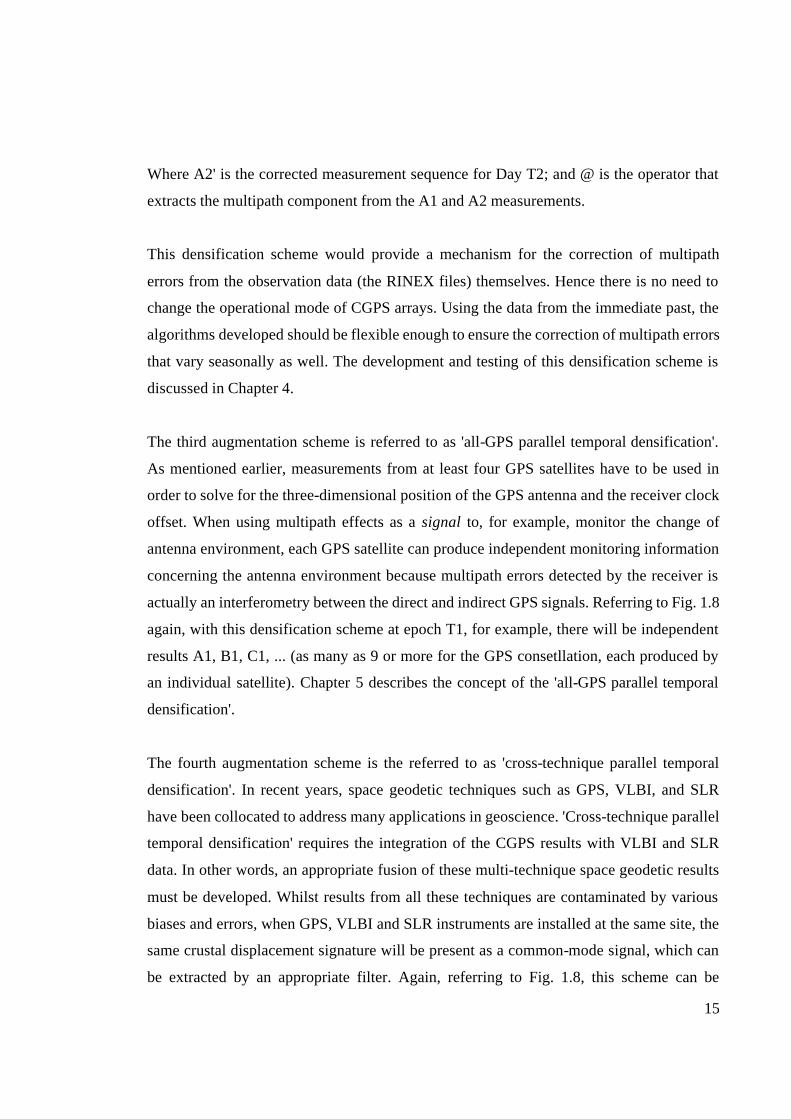
Where A2' is the corrected measurement sequence for Day T2; and @ is the operator that

extracts the multipath component from the A1 and A2 measurements.

This densification scheme would provide a mechanism for the correction of multipath

errors from the observation data (the RINEX files) themselves. Hence there is no need to

change the operational mode of CGPS arrays. Using the data from the immediate past, the

algorithms developed should be flexible enough to ensure the correction of multipath errors

that vary seasonally as well. The development and testing of this densification scheme is

discussed in Chapter 4.

The third augmentation scheme is referred to as 'all-GPS parallel temporal densification'.

As mentioned earlier, measurements from at least four GPS satellites have to be used in

order to solve for the three-dimensional position of the GPS antenna and the receiver clock

offset. When using multipath effects as a signal to, for example, monitor the change of

antenna environment, each GPS satellite can produce independent monitoring information

concerning the antenna environment because multipath errors detected by the receiver is

actually an interferometry between the direct and indirect GPS signals. Referring to Fig. 1.8

again, with this densification scheme at epoch T1, for example, there will be independent

results A1, B1, C1, ... (as many as 9 or more for the GPS consetllation, each produced by

an individual satellite). Chapter 5 describes the concept of the 'all-GPS parallel temporal

densification'.

The fourth augmentation scheme is the referred to as 'cross-technique parallel temporal

densification'. In recent years, space geodetic techniques such as GPS, VLBI, and SLR

have been collocated to address many applications in geoscience. 'Cross-technique parallel

temporal densification' requires the integration of the CGPS results with VLBI and SLR

data. In other words, an appropriate fusion of these multi-technique space geodetic results

must be developed. Whilst results from all these techniques are contaminated by various

biases and errors, when GPS, VLBI and SLR instruments are installed at the same site, the

same crustal displacement signature will be present as a common-mode signal, which can

be extracted by an appropriate filter. Again, referring to Fig. 1.8, this scheme can be

16

understood by assuming that A1, A2, ... are the GPS results, whilst B1, B2, ... the VLBI

results, and C1, C2, ... the SLR results. This scheme is discussed in Chapter 6.

So far all the augmentation schemes fall into the 'temporal densification' category. The next

two augmentation schemes, however, are 'spatial densification' techniques. Spatial

densification will augment CGPS's capability in resolving spatially high frequency features

of crustal deformation. Moreover, even when the CGPS networks are densified in order to

recover the signature of the deformation, the station configuration design may not be ideal.

As shown in Fig. 1.9, suppose that all the measurements are taken at epoch T.

At time T

Latitude

(A 1 , B 1 ) (A 2 , B 1 )

ϕ 1 ϕ 2

(C, B 1 )

(A 1 , B 2 ) (A 2 B 2 ) (C, B 2 )

(A 1 , D) (A 2 D) (C, D)

λ 1

λ 2

Longitude

(A d B d2

)

,

,

,

Figure 1.9 Spatial densification schemes.

The fifth augmentation scheme is 'soft spatial densification'. In this scheme CGPS is

integrated with techniques such as differential Synthetic Aperture Radar Interferometry

(InSAR) (the word "soft" is used because no additional GPS hardware installation is

needed). Since data from CGPS arrays (GPS measurements collected at sites denoted by

(Ai, Bj), where i, j = 1, 2 in Fig. 1.9) can be used to map tropospheric water vapour and

ionospheric disturbances, these results can be used to remove atmospheric biases in InSAR.

With the support of SLR and VLBI, GPS coordinates can be considered as being 'absolute'

in the sense that they are tied to a well-defined terrestrial reference system. By assuming

that there are no displacements at a few points (reference points) in a radar image, InSAR

results are essentially relative measurements. GPS measurements on the reference points

17

(Ai, Bj) in a SAR image can also be used as constraints to mitigate the influence of SAR

satellite orbit errors. On the other hand, InSAR, with its high spatial resolution (25m in the

case of ERS-2), can be used to densify GPS results in a spatial sense. The densified

measurements are (Ai, D), (C, Bj), and (C, D) in Fig. 1.9. Therefore, the CGPS and InSAR

techniques are very complimentary. The integration of CGPS with InSAR is discussed in

Chapter 7.

The sixth and last augmentation scheme is concerned with 'hard spatial densification' (the

word "hard" is used because in this scheme additional GPS hardware has to be installed).

'Hard spatial densification' can be achieved either by deploying a sub-network of low-cost

GPS receivers (located at (Ai, D), (C, Bj), and (C, D)), to in-fill the present CGPS arrays

(located at (Ai, Bj) where i, j = 1, 2 in Fig. 1.9). This typically involves the integration of

single-frequency and dual-frequency GPS receivers in a so-called ‘inward hard spatial

densification’. Alternatively, by deploying receivers at some geophysically 'strategic' sites

located at (Ad, Bd) outside the existing CGPS array located at (Ai, Bj), so that

combinations of different baselines can be used to, for example, separate plate tectonic and

seismic fault movements, in a so-called ‘outward hard spatial densification’. The

development and testing of hard densification schemes is described in Chapter 8.

These augmentations can be used either independently or collectively, depending on the

resources available in a CGPS array, and at a specific site. For example, the retro-

densification and the all-GPS densification can be carried out at the same time; the retro-

densification result can be used as an input to the GPS-VLBI-SLR cross-technique

densification; the cross-technique densification results can be used instead of the GPS-only

result in the soft densification with InSAR; the soft densification and the hard densification

can verify each other; and so on.

This thesis consists of 9 chapters. This chapter presents the background to GPS and CGPS.

The research motivation, the methodology, and contributions of this research work are also

outlined. In Chapter 2 the mathematical basis for this research, the adaptive filter based on

the least-mean-square algorithm, is developed. Chapters 3 to 8 deal with each of the CGPS

18

densification schemes outlined above. Chapter 9 contains the summary, conclusions and

recommendations arising from this research.

1.7 Contributions of the Research

While 'augmentations' are often used for GPS navigation applications, this research

systematically studies the augmentations to continuous GPS networks/processing for

crustal deformation monitoring applications. The four temporal densification schemes

based on: high rate GPS-RTK, GPS multipath effects, and collocated VLBI and SLR, to

augment the CGPS networks are the most significant contributions of this research. In

addition, the two spatial densification schemes are also important new findings. The

contributions of this research can be summarized as follows:

• The 'serial temporal densification scheme', in an attempt to use GPS as a

seismometer, has been developed and tested. Simulated seismic signals have been

extracted from very noisy, high rate (10Hz and 20Hz) GPS-RTK results, using an

adaptive filter based on the least-mean-square algorithm. The extracted results are in

very good agreement with those of collocated traditional seismometers. The

proposed technique can also be used for other applications, such as the monitoring

of tsunami and the deformation of large engineering structures.

• The proposed 'retro-active temporal densification scheme' takes advantage of the

fact that the GPS multipath disturbance has a periodic characteristic (and is repeated

between consecutive sidereal days). This densification scheme provides a means of

correcting for multipath errors in the observation data themselves.

• The proposed 'all-GPS parallel temporal densification scheme' uses the multipath

effects as a signal to, for example, monitor any change in the antenna environment.

Each GPS satellite contributes an accurate, independent measure of the surrounding

environment, because the multipath detected by the GPS receiver is actually an

19

interferometry between the direct and indirect GPS signals. Models relating the

change of multipath to a change in the antenna environment have been derived.

• The proposed 'cross-technique parallel temporal densification scheme' integrates

collocated CGPS, VLBI and SLR results. Whilst results from all these techniques

are contaminated by various biases and errors, when GPS, VLBI and SLR

instruments are installed at the same site, the same crustal displacement signature

presents as a common-mode signal.

• The proposed 'soft spatial densification scheme' integrates CGPS with the InSAR

technique. The Double Interpolation and Double Prediction (DIDP) approach has

been developed, and combines the advantage gained from high temporal resolution

(of the CGPS measurements) and with the high spatial resolution (of the InSAR

result) for the same region. DIDP can generate deformation monitoring products of

high resolution, in both a temporal and spatial sense. Quality assurance measures

have also been developed for DIDP.

• A 'hard spatial densification scheme' has been developed and tested. There are two

scenarios. One involves the deployment of a sub-network of single-frequency GPS

receivers to in-fill an existing CGPS array using concept known as ‘inward hard

spatial densification’. The other requires the deployment of receivers at some

geophysically strategic sites outside an existing CGPS array, in the form of an

‘outward hard spatial densification’. The 'inward hard spatial densification' has

been demonstrated to be a cost-effective approach to improving the CGPS spatial

resolution and to providing some redundancy in hazardous environments such as

active volcanoes. In the case of 'outward hard spatial densification', receivers can be

used more efficiently to form combinations of different baselines which can, for

example, separate plate tectonic and seismic fault movements.

These augmentations can be used either independently or collectively depending on the

resources available in a CGPS array and at a specific site.

20

Conventional signal processing systems for the extraction of information from an incoming

signal operate in an open-loop fashion. That is, the same processing function is carried out

in the present time interval regardless of whether that function produced the correct result

in the preceding time interval. In other words, conventional signal processing techniques

make the basic assumption that the signal degradation is a known and time-invariant

quantity.

Adaptive processors, on the other hand, operate with a closed-loop (feedback) arrangement.

The incoming signal x(n) is filtered or weighted in a programmable filter to yield an output

y(n) which is then compared against a desired, conditioning or training signal, d(n), to

yield an error signal, e(n). This error is then used to update the processor weighting

parameters (usually in an iterative way) such that the error is progressively minimized (i.e.,

the processor output y(n) more closely approximates the desired signal d(n)). Such

processors fall into the class of adaptive filters.

Adaptive filters, which are the mathematical basis of this research, are concerned with the

use of a programmable filter whose frequency response or transfer function is altered, or

adapted, to pass without degradation the desired components of the signal and to attenuate

the undesired or interfering signals, or to reduce any distortion on the input signal. These

adaptive filters are frequently used to recover signals from channels whose characteristic is

time varying.

Much of the early work on adaptive filters was arrived at by independent study in different

organizations. Notable early developments occurred at the Technische Hochschule

Karlsruhe in Germany and at Stanford University, where adaptive pattern recognition

systems were initiated in 1959 (Rudin, 1967). Collaboration in 1964 between these

institutions produced a comparative evaluation of their respective techniques which

2 ADAPTIVE FILTER AND ASSOCIATED SIMULATION STUDIES

21

subsequently led to the development of the most widely used algorithm for processor

weight adjustment. Further relevant work was being conducted simultaneously at the

Institute of Automatics and Telemechanics in Moscow. Now applications of adaptive filters

can be found in such diverse fields as speech analysis, seismic, acoustic, and radar signal

processing, and digital filter design (e.g. Haykin, 1996; Proakis & Mandakis, 1996; Solo &

Kong, 1995).

2.1 The Adaptive Filter

An adaptive filter used for noise suppression is a dual-input, closed-loop adaptive feedback

system. The operation of such an adaptive filter involves two basic processes: 1) a filtering

process to produce an output in response to an input sequence; and 2) an adaptive process

for the control of adjustable parameters used in the filtering process.

In the present application the dual-inputs to the adaptive filter are the primary input d(n)

and the reference input x(n), which have sample size (vector length) N. The primary input

d(n) consists of the desired signal of interest s(n) buried in (or contaminated by) noise x’(n),

that is

d(n) = s(n) + x’(n) (2.1) The reference input x(n) supplies noise alone. In order to obtain a relatively noise-free

signal using the adaptive filter output, s(n), x’(n), and x(n) have to satisfy the following

conditions:

1) the signal and noise in the primary input are uncorrelated with each other, that is

E[s(n)x’(n-k)] = 0 n,k=0, …, N-1 (2.2) Where E[ . ] denotes the expectation operator.

2) the noise in the reference input is uncorrelated with the signal s(n) but is correlated

with the noise component of the primary input x’(n), that is

E[s(n)x(n-k)] = 0 n,k=0, …, N-1 (2.3) and

22

E[x(n)x’(n-k)] = p(k) n,k=0, …, N-1 (2.4) where p(k) is an unknown cross-correlation for lag k.

2.2 The Filter Design

There are several types of programmable filters that can be used in the design of the

adaptive filters. Here two basic filter designs are introduced briefly.

The most generalized digital filter structure is the recursive filter design, which comprises

both feedforward and feedback multipliers, whose weight are controlled by some

coefficients. The response of this filter is governed by the difference equation which shows

that the value of the present filter output sample is given by a linear combination of the

weighted present and past input samples as well as the previous output samples. This

structure results in a pole-zero filter design where the pole locations are controlled by the

feedback coefficients and the zero locations by the feedforward coefficients. The number of

poles and zeros, or order of the filter, is given by the number of delay stages.

This recursive structure has theoretically an infinite memory and hence it is referred to as

an infinite impulse response (IIR) filter design. It is not unconditionally stable unless

restrictions are placed on the values of the feedback coefficients. However, the inclusion of

poles as well as zeros makes it possible to realize sharp cutoff filter characteristics

incorporating a low transition bandwidth with only a modest number of delay stages (i.e.,

low filter complexity). One drawback of the IIR design is that no control is offered on the

phase (group delay) response of the filter. However, the major problem with adaptive IIR

filter design is the possible instability of the filter due to poles straying outside the stable

region.

One way to overcome the drawback of potential instability in the filter is to design an all-

zero filter which uses only feedforward multipliers and is unconditionally stable (Fig. 2.1).

This has only a limited memory, which is controlled by the number of delay stages and it

results in the finite impulse response (FIR) filter design. The input signal is delayed by a

number of delay elements, which may be continuous but usually are restricted to discrete

23

values. The outputs of these time-delay elements are subsequently multiplied by a set of

stored weights and the products summed to form the output signal. This implies that the

output is given by the convolution of the input signal with the stored weights or impulse

response values. This filter incorporates only zeros (as there are no recursive feedback

elements) and hence a large number of delay elements are required to obtain a sharp cutoff

frequency response. However, the filter is always stable and can provide a linear-phase

response.

Therefore, the Finite-duration Impulse Response (FIR) filter (Haykin, 1996), which is also

known as a tapped-delay line filter, transversal filter, all-zero filter, or moving-average

filter, is employed in this application due to its stability, versatility and ease of

implementation.

As indicated in Fig. 2.1, the FIR consists of three basic elements:

• the unit-delay elements identified by the unit-delay operator z −1 , where the number

of elements M refers to the filter length (its order is M-1);

• the multipliers, whose function is to multiply the tap input by a filter coefficient (tap

weight); and

• the adders, which sum the individual multiplier outputs and yield an overall filter

output:

y(n) = wi

^

i= 0

M −1

∑ (n)x(n − i) (2.5)

where M is the length of the adaptive FIR filter, w ni

^

( ) denotes a time-varying transfer

function (tap weight), which changes, or adapts, according to signal conditions, under the

control of an algorithm which will be described in the next section.

24

Figure 2.1 The FIR filter scheme.

2.3 The Adaptive Algorithm Design

In an adaptive system an absolute minimum of a priori information is necessary about the

reference signal. The adaptive filter operates by estimating the statistics of the reference

signal and adjusting its own response in such a way as to minimize some ’cost function’.

This cost function may be derived in a number of ways depending on the intended

application, but normally it is derived by the use of the primary (or desired) signal. The

most commonly used cost function is the least-mean-squares (LMS) function. Alternatives

are functions such as modulus of error and nonlinear threshold functions. The task of the

adaptive algorithm is to adjust the weights in the programmable filter in such a way as to

minimize the difference or error e(n) between the processor output y(n) and the primary

input d(n).

Many methods exist to adjust the filter weight values to obtain the optimum solution.

Random perturbation techniques have been applied, where the weights are altered and the

output is examined to ascertain whether the random perturbation moves it toward or away

from the desired solution. The least-mean-square (LMS) algorithm was first formally

reported by Widrow (1971). It is now widely applied to the calculation of the adaptive filter

weights, as it uses gradient search techniques, which converge toward the optimum solution

much more efficiently than do other algorithms. It will be shown that this algorithm can

maximize signal-to-noise ratio.

25

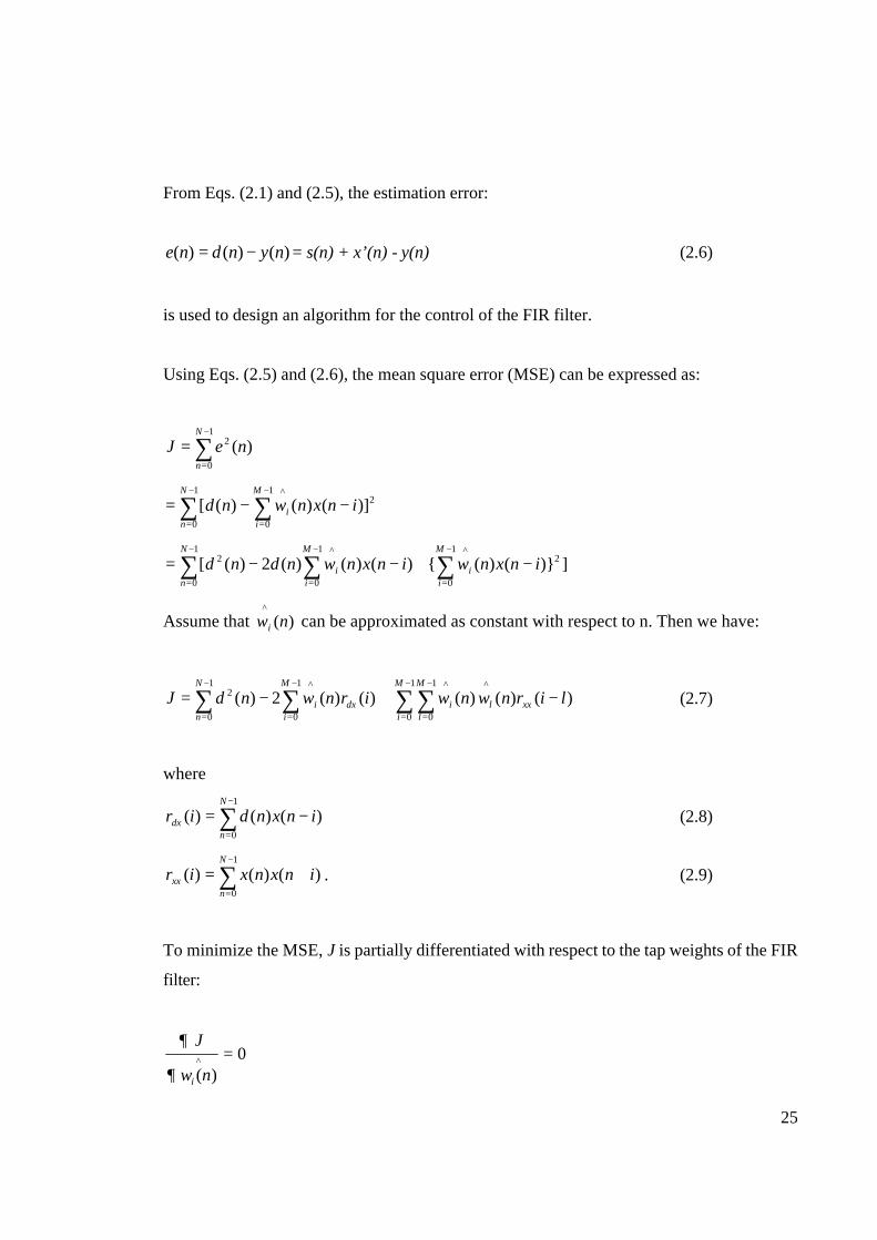
From Eqs. (2.1) and (2.5), the estimation error:

e n d n y n( ) ( ) ( )= − = s(n) + x’(n) - y(n) (2.6)

is used to design an algorithm for the control of the FIR filter.

Using Eqs. (2.5) and (2.6), the mean square error (MSE) can be expressed as:

)(1

0

2 neJN

n∑

−

=

=

21

0

1

0

^

)]()()([ inxnwndN

n

M

ii −−= ∑ ∑

−

=

−

=

])}()({)()()(2)([ 21

0

^1

0

^1

0

2 inxnwinxnwndndM

ii

M

ii

N

n

−+−−= ∑∑∑−

=

−

=

−

=

Assume that )(^

nwi can be approximated as constant with respect to n. Then we have:

)()(2)(1

0

^1

0

2 irnwndJ dx

M

ii

N

n∑∑

−

=

−

=

−= )()()(^1

0

1

0

^

lirnwnw xxl

M

i

M

li −+ ∑∑

−

=

−

=

(2.7)

where

∑−

=

−=1

0

)()()(N

ndx inxndir (2.8)

∑−

=

+=1

0

)()()(N

nxx inxnxir . (2.9)

To minimize the MSE, J is partially differentiated with respect to the tap weights of the FIR

filter:

0)(

^ =nw

J

i∂

∂

26

which is equivalent to:

l =0

M−1

∑ w l

^

(n)rxx (i − l) = rdx(i) , i=0, …, M-1 (2.10)

This yields the set of linear equations that generate the optimum filter coefficients at time n.

To solve the equations, both the auto-correlation sequence { r ixx ( ) } of the reference

sequence {x(n)} and the cross-correlation sequence { r idx ( ) } between the primary sequence

{d(n)} and the reference sequence {x(n)} are required.

The signal s(n) is part of the error signal e(n) and the noise component in the adaptive filter

output is x’(n) - y(n), as indicated in Eq. (2.6). While s(n) is essentially unaffected by the

filter, minimizing E is equivalent to minimizing the output noise x’(n) - y(n). Therefore, the

signal-to-noise ratio of the output signal is maximized.

There are two special cases when applying the adaptive filter:

1) The adaptive filtering is perfect when y(n) = x’(n), and in this case the system output is

noise-free, as can be seen from Eq. (2.6).

2) The adaptive filtering will be switched off automatically, as can be seen from Eq. (2.10),

when the reference signal x(n) is completely uncorrelated with both the signal s(n) and the

noise component x’(n) of the primary signal d(n), i.e., E[d(n)x(n-k)] = 0 for n,k=0, …, N-

1. In this case, the primary signal is left intact and the output signal-to-noise ratio remains

unchanged.

2.4 The Real-time Implementation of the Adaptive Filter

As mentioned above, in order to solve the equations, both the auto-correlation sequence

{ r ixx ( ) } of the reference sequence {x(n)} and the cross-correlation sequence { r idx ( ) }

27

between the primary sequence {d(n)} and the reference sequence {x(n)} have to be

calculated, which is almost impossible in real-time applications. Therefore the simplified

least-mean-square (LMS) algorithm has been introduced as an alternative computational

method to adaptively adjust the coefficients (weights) of an FIR filter, w ni

^

( ) , as in the

following equation (tap-weight adaptation ):

)()()()(^

1

^

inxnenwnw ii −+= − µ (2.11)

where µ is the step-size parameter, i = 0, …., M-1 and n = 0,…,N-1. In order to facilitate the comparison of Eqs. (2.10) and (2.11), the following matrix-vector

notations are defined:

XT(n) = [x(n) x(n-1) ... x(n-M+1)]

WT(n) = [ )(0

^

nw )(1

^

nw ... )(1

^

nwM − ] P = E[d(n) X(n)] R = E[X(n)XT(n)] where the matrix transpose is defined by the superscript T. Then Eqs. (2.5) and (2.6) can be rewritten as: y(n) = W(n) XT(n) = X(n) WT(n) (2.5a) e(n) = d(n) - W(n) XT(n) = d(n) - X(n) WT(n) (2.6a) The cost function (or performance function) expressed in Eq. (2.7) can be rewritten as: J = E[e2(n)] = D - 2 WT(n)P + WT(n) RW(n) (2.7a) where D is the expected power of d(n): D = E[ |d(n)| 2]

28

Note that J is a quadratic function of the weight vector W(n). The gradient of J becomes:

W

J

∂

∂ = 2 (RW(n) – P) (2.8a)

The solution of the optimal weight vector Wopt can be obtained by:

W

J

∂

∂ = 0

i.e., Wopt = R-1P (2.10a) On the other hand, the real-time LMS algorithm is using the squared-error as the cost

function, i.e.,

G = e2 (n) The gradient of G becomes:

W

G

∂

∂ = 2 e(n)

W

ne

∂

∂ )(

= -2 e(n) X(n) This instantaneous gradient has been used in the real-time version of LMS to form an

adaptive filtering algorithm which approximate a true gradient search of the cost function in

the following:

W(i) = W(i-1) + µe(i) X(i) (2.11a) Note that

E[W

G

∂

∂] = E[-2 e(n) X(n)]

= 2 E[ - (d(n) - W(n) XT(n)) X(n)] = 2 (RW(n) – P)

29

= W

J

∂

∂

Thus the expected value of the approximate gradient equals the true gradient. Therefore, it

has been shown that the LMS algorithm expressed in Eq. (2.11) can minimize the sum of

squared errors as in the case of Eq. (2.10). Evidence has also been presented on the model-

independence, and hence robust performance of the LMS algorithm (Solo & Kong, 1995),

making the LMS algorithm the most widely known and used adaptive algorithm.

2.5 Evaluation of the LMS Algorithm

In this section, the solutions developed earlier for the optimal weight vector are used to add

some intuitive insight into what the cost function J means and how the optimal weight

vector depends on the characteristics of x(n) and d(n).

From Eqs. (2.7a) and (2.10a), the minimum value of J as the weight vector satisfies the normal equation can be found as: Jmin = D - 2 WT

opt P + WTopt RWopt

= D - 2 WTopt P + WT

opt P = D - WT

opt P Thus the minimum value of J depends on D (the power or energy of d(n)), on the optimal

weight vector Wopt and on P (the cross-correlation between d(n) and X(n)).

Given this minimum value, it is interesting to konw how large a price in performance is

paid by not using the optimal vector. In particular, let W(n), the actual weight vector, be

defined by:

W(n) = Wopt + V

Where V is an M-dimensional vector representing the difference between W(n) and Wopt .

Substituting this value of W(n) into Eq. (2.7a), we find that:

30

J = D - 2 (WTopt + VT)P + (WT

opt + VT) R (Wopt + V)

= D - 2 WTopt P + WT

opt R Wopt - 2VTP + WTopt R V + VT R Wopt + VT R V

= Jmin - 2VTP + PT V + VT P + VT R V

= Jmin + VT R V

This is the key result and forms the basis for much intuition about optimal squared error

filters. It states that any excess squared error is a quadratic function of the difference

between the actual weight vector W(n) and the optimal one Wopt. Because VT R V is never

negative, Jmin is in fact the minimum attainable value. For most well-behaved problems

VTRV is always positive for nonzero V, meaning that any difference between W(n) and

Wopt , hence nonzero V, will result in J being greater than the minimum possible value.

Note that the penalty for poor choice of W(n) depends only on the reference input x(n) and

not on the primary input d(n). Thus the character of the reference input affects the nature of

the solution. Therefore, it is vital to choose an appropriate signal as the reference input.

2.6 Implementing Issues of the Adaptive Filter

However, special attention has to be paid to two closely related issues: the choice of

suitable value for the step-size parameter µ , and the filter length M.

1) It is important to select an appropriate µ which controls the rate of convergence of the

LMS algorithm to the optimum solution. The larger the µ selected, the faster the

convergence. However, too large a value of µ may result in the LMS algorithm becoming

unstable. To ensure stability, µ should be in the range (Proakis, 1995):

01

10< <µ

MPx (2.12)

where M is the length of the adaptive FIR filter and Px is the power of the reference signal,

which can be approximated by:

31

Px ≈1

1+ Mx2

n= 0

N −1

∑ (n) =rxx(0)

M + 1 (2.13)

where rxx ( )0 is the auto-correlation function of the reference sequence for zero lag.

2) The filter length (i.e., the number of independently adjusted parameters in the filter)

should be selected so that the filter best models the regular features of a set of input data.

The Minimum Description Length (MDL) criterion (Haykin, 1996) has been employed in

this application. It is defined as:

MDL(M) = - L(θ^

M ) + 12 M lnN (2.14)

where M is the filter length, N is the length of the input sequence, and L(θ^

M ) is the

logarithm of the maximum likelihood estimates of the filter parameters. The first term in

the above equation tends to decrease rapidly with increasing M, while the second term

increases linearly with increasing M. Therefore there is a value of M which can minimize

MDL, representing the optimum length of the filter.

2.7 Adaptive Filtering of Simulated Data

When the FIR filter and the adaptive algorithm are integrated, an adaptive filter as shown in

Fig. 2.2 is obtained. In this section, numerical simulation data are used to explore the

features of such an adaptive filter, before applying it to the processing of CGPS results.

32

Figure 2.2 Adaptive filtering configuration.

Though ideally “true” noise has to be used as a reference signal in order to cancel it from

the primary signal as discussed in previous sections, to derive true noise is as difficult as

deriving a true signal for many practical applications. In fact, there are no fundamental

differences between “signal” and “noise”, except that a “signal” is a desired output and a

“noise” is an undesired one. To address practical applications of the adaptive filter it is

necessary to introduce the terms “coherent component” and “incoherent component” when

discussing the compositions of the primary and reference signals. A “coherent component”

is a composition of the primary signal which is correlated with a composition of the

reference signal, while an “incoherent component” is a composition of the primary signal

which is uncorrelated with any composition of the reference signal. In Fig. 2.2, the

“coherent component” is the direct output of the FIR filter, and the “incoherent component”

is the output of the whole adaptive filtering system.

In the case of CGPS measurements, the time series on a selected day can be expressed as:

)(')(')( nxnsnr += (2.15)

33

where s n' ( ) is the crustal deformation (signal free of multipath, etc.) and )(' nx is the noise

contribution respectively. And n is the epoch number.

The time series on the next day is expressed as:

)()()( nxnsnd += (2.16)

where s n( ) and )(nx are analoguous to s n' ( ) and )(' nx .

From previous studies (e.g. Han & Rizos, 1997), )(nx and )(' nx are highly correlated in

terms of multipath in nearly static antenna environments. But s n( ) and s n' ( ) are

uncorrelated, which means that the adaptive filtering conditions are only partially satisfied

(a correlation between s n( ) and s n' ( ) may become detectable in some stations caused, for

example, by temperature expansion). In this case, can the adaptive filter be used to remove

noise such as multipath from the results of the second day by employing the results of the

first day as a reference signal?

As discussed in previous sections, and also in Ge (1999), there are two special cases to be

considered in the application of an adaptive filter. Eq. (2.15) can be treated as a linear

combination of the two cases. Therefore, theoretically it is possible to mitigate noise such

as multipath by using CGPS results of two adjacent days as inputs to an adaptive filter.

Numerical simulation studies are carried out in order to demonstrate the feasibility of such

filter schemes, and to explore some of the characteristics of the adaptive filter. In the first

simulation both the reference (r(n)) and primary (d(n)) signals are composed of two sine

waves, and all the components of r(n) and d(n) are uncorrelated:

r(n) = 10 cos(nπ/8+2)+25 cos(nπ/3);

d(n) = 25 cos(nπ/10+π)+10 cos(nπ/5);

where π=3.14159; r(n) and d(n) are in mm; n is the sample number and the sampling

interval is 1 second.

34

Fig. 2.3 is the result of this simulation. It can be seen from both the time series and their

Fast Fourier Transform (FFT) spectrum that although the coherent component is not zero,

as it should be, the incoherent component is indeed left intact. Please note that the vertical

scales of the coherent component plots are –5 to 5 for amplitude and 0 to 4*103 for the FFT

power respectively.

In the second simulation both the reference (r(n)) and primary (d(n)) signals are composed

of two sine waves and the 0.05Hz component 25*cos(n*π/10+π) in d(n) is introduced as

the coherent component, and the 0.1Hz component 10*cos(n*π/5) as the incoherent

component (note also that the phase difference π - 2 has been introduced on purpose

between the two coherent components in d(n) and r(n)):

r(n) = 10*cos(n*π/10+2)+25*cos(n*π/3);

d(n) = 25*cos(n*π/10+π)+10*cos(n*π/5);

Fig. 2.4 is the result of this simulation. It can be seen from both the time series and their

FFT spectrum that the coherent and the incoherent components of d(n) are successfully

separated, despite that there is a phase difference between the two coherent components in

d(n) and r(n).

To summarize the numerical simulation results, a truth table for adaptive filtering is

presented in Table 2-1. From the table it can be concluded that the adaptive filter can be

used as a powerful signal decomposer (analyser).

Table 2-1 Truth table for adaptive filtering.

Primary & reference

x, x’ uncor. s, s’ corr.

x, x’ corr. s, s’ uncorr.

x, x’ uncor. s, s’ uncorr.

Coherent s x ≅ 0 Incoherent x s s+x

In the following chapters, the adaptive filter based on the least-mean-square algorithm will be used in various CGPS densification schemes.

35

Figure 2.3 Numerical simulation result of adaptive filtering of uncorrelated signals.

36

Figure 2.4 Numerical simulation result of adaptive filtering of partially correlated

signals.

37

Serial temporal densification is realised by increasing the data sampling rate of GPS

receivers and applying appropriate signal filtering techniques. It is typical that GPS

receivers in CGPS networks typically make one set of measurements every 30 seconds.

However, it is comparatively easy to increase this data rate to one sample per second (1Hz),

since all currently deployed GPS receivers can support this rate (though the volume of data

will be increased substantially!). Refer to Fig. 1.7 again, this 1Hz rate is equivalent to

extend the dashed-line rectangle (the coverage of the current CGPS) in the negative

direction of the vertical axis to 1 second. If it has to be further extended to 0.1 second, new

receivers such as the Leica CRS1000 or Trimble MS750 would have to be introduced to

satisfy the 10-20Hz sampling rate requirement for the detection of ground motion due to

e.g. seismic waves (Ge, 1999).

Even with high sampling rates, the challenge still is to resolve the very weak signal from

the noisy ‘kinematic' GPS solutions. This Chapter, focusing on the temporal densification

and using the GPS seismometer concept to facilitate the discussion, starts with an

introduction to GPS Real-Time Kinematic (RTK) applications. Two experiments are

described in detail, that demonstrate a serial temporal densification scheme using the GPS

RTK system as a 'GPS seismometer'. The last section of this Chapter discusses the

implemention issues involved in using GPS as a seismometer.

3.1 GPS Real-Time Kinematic (RTK) Applications

3.1.1 Standard RTK

The standard GPS Real-Time Kinematic (RTK) technique is a relative (differential)

positioning procedure whereby carrier phase measurements (or corrections) are transmitted

in real-time from a reference or base station to a user's mobile receiver. Centimetre

3 SERIAL TEMPORAL DENSIFICATION – THE 'GPS SEISMOMETER'

38

accuracy is achieved without the need to record and post-process double-differenced carrier

phase observables. The resolution of the carrier cycle ambiguities on-the-fly (OTF) is the

key to modern RTK techniques. Due to the fact that atmospheric conditions can change

rapidly, residual ionospheric and tropospheric biases (remaining after double-differencing

the data) will grow in magnitude with increasing receiver separation. Hence the typical

'allowable' distance between user and base station receivers for OTF-RTK is only up to

10km. In the case of an instrument like the MS750 (Trimble, 2000), the stated accuracy is 1

cm+2ppm horizontal and 2cm+2ppm vertical in the so-called 'synchronized' RTK mode,

and 2cm+2ppm horizontal and 3cm+2ppm vertical when used in the low latency mode. As

will be seen in Section 3.5.1, this limitation is a serious concern when attempting to

implement a 'GPS seismometer' based on the RTK positioning mode.

3.1.2 Network RTK (the Virtual Reference Station concept)

Standard (or traditional) GPS-RTK positioning is limited with respect to the distance

between the reference station and the user receiver. CGPS networks such as the GEONET

are able to provide services for traditional RTK positioning, but only because the residual

systematic biases are relatively small due to the fact that the network of reference stations is

very dense. However, the desired density of reference stations is a function of such factors

as the 11 year solar sunspot cycle, with interstation distances being allowed to increase

during solar minima, and decrease during solar maxima.

The concept of 'virtual reference stations' (VRS) is an effective way of eliminating/reducing

systematic errors in reference station data, and hence allows for an increase in the distance

between CGPS reference stations, while increasing the reliability of the RTK technique and

reducing the initialization time. The 'virtual reference station' concept was first

commercialized in Spectra Precision's GPS-Network software (Terrasat, 2000), although

there have been many trials of similar systems over the last five years. Such network-based

RTK systems require continuous modem line connections between the control centre and

39

all reference stations. GPS raw data is transmitted continuously to the centre. The control

centre then performs the following standard tasks:

• Data archiving of all receivers in the RINEX format;

• Compression of RINEX files if required;

• Data quality analysis of the received GPS data;

• Visualization of remote station status; and most importantly

• Continuous computation of the systematic errors (mainly ionospheric biases,

tropospheric biases, ephemeris errors and carrier phase ambiguities for L1 and L2) by

analyzing the double-differenced carrier phase observations.

From these network results the interpolated systematic error for a specific user within the

area defined by the reference station network can be estimated. The estimated systematic

error when applied to the RTK processing overcomes the problems of distance-dependent

errors. The interpolation requires an approximate position of the user receiver. The standard

NMEA strings of the GGA message, which all major receivers provide, can be used for this

purpose (it is a basic navigation solution using pseudo-range data). Hence, any off-the-shelf

single- or dual-frequency GPS receiver capable of performing RTK positioning can be used

without modification. From this position an 'optimized' RTCM data stream can be

generated and input to the user receiver. Because this process is equivalent to creating raw

reference station data for the approximate user position, it is often referred to as the

"Virtual Reference Station (VRS)" technique. With these optimized RTCM messages it is

possible to perform improved RTK positioning within the reference station network. Yet

another approach is to simply create the VRS raw data itself. Position errors of 1-3cm

horizontal and 4-6cm vertical using reference stations spaced at distances of approximately

50 km have been reported by Bücherl et al. (2000). Better accuracy for VRS-RTK is

expected with advancs in receivers and orbit products (such as the use of IGS Ultra rapid

products (IGSCB, 2000)). Another advantage of the VRS is the almost uniform accuracy,

regardless of the distance of the user from any one reference station.

40

A VRS-RTK system connecting 85 stations from Switzerland, Finland, Sweden, and

Germany is currently operating (Terrasat, 2000). A system implementing the Virtual

Reference Station concept, Internet-connected reference station network and TV sound

multiplexed sub-carrier data link has also been tested in Tokyo, Japan (Petrovski et al.,

2000). This network covers a region of approximately 100 km in radius. Many more VRS-

RTK system are likely to be installed in several regions and cities over the next few years.

As will be seen in Section 3.5.1, the VRS-RTK provides a good basis for implementing a

'GPS seismometer' based on the RTK technique.

3.2 GPS Seismometer – an Overview

The large near-field displacements before and during an earthquake are invaluable

information for earthquake source study and for the detection of slow/silent quakes or pre-

seismic crustal deformation events. However, none of the current seismometers can

measure large near-field displacements directly. Typically, a seismometer (or seismograph)

employs a pendulum to record seismic waves, because an "ideal pendulum" always stays in

its original position regardless of the movements of the seismometer. Because the GPS

satellites are not affected by earthquakes, the GPS constellation can be considered an "ideal

pendulum". Therefore, a GPS receiver on the Earth can be used as a seismometer if its

sampling rate is high enough to recover the signature of the antenna displacement.

Accurate time synchronization for seismic networks is vital for the determination of

earthquake hypocentres. With no exact time, the seismic records are, as a rule, useless.

Therefore, GPS has been widely used for accurate time-stamping of data collected by

seismic networks. However, only recently have GPS receivers achieved very high data

sampling rates. State-of-the-art GPS receivers with 10 to 20Hz sampling rates are now

available (Leica, 2000; Timble, 2000). This means that such GPS receivers may be able to

reproduce signals with frequencies from 0 HZ to (say) 10Hz, which is already compatible

with some current seismic networks such as TERRAscope, a wide dynamic range, broad-

41

band (10 Hz to 0 HZ) seismographic network funded by the L. K. Whittier, ARCO

Foundation and NSF/ARI, USA (Caltech, 2000). Hence, the concept of a 'GPS

seismometer' appears feasible.

Is there a need for a 'GPS seismometer'? The largest amplitude of vibration accompanying

an earthquake reported so far is 180mm for the 1923 Tokyo Quake, and the fault

displacements associated with the largest earthquakes are of the order of 30m (Turcotte,

1982). Despite advancements in seismometer design, it is now still true, as Dr. Branson has

claimed, that “Very probably, there have been earthquakes of larger movements which our

seismographs were unable to record” (Branson & Tarr, 1952). As a matter of fact, though

great efforts have been made to develop highly dynamic seismometers using the latest

electronic technology, direct measurement of large co-seismic displacements with a flat

frequency response remains elusive. The result is likely to be an under-estimation of

earthquake sources. The development of a 'GPS seismometer' is therefore an option worth

considering.

The first experiment concerning GPS seismometers was reported as early as 1994. It was

carried out by the Disaster Prevention Research Institute (DPRI), Kyoto University, Japan

(Hirahara et al., 1994). The experiment was performed at a user site equipped with a GPS

antenna on a slider, and two reference sites at distances 160m and 160km away from this

site. The slider oscillated horizontally with periods of 25-300sec and amplitude of 15cm.

The sampling interval of the receivers was 1sec. A horizontal accuracy of 1-2cm was

achieved in post-processing, and it was concluded that using GPS as a strain seismometer

to obtain large amplitude, near-field ground motion was possible.

Another GPS seismometer experiment was carried out by the Geographical Survey Institute

(GSI) of Japan, involving the kinematic processing of some GEONET data to derive

ground motion due to the 4 October 1994, M8.1 Hokkaido-Toho-Oki earthquake (Hatanaka

et al., 1994). The sampling rate of this continuous GPS (CGPS) data was 30sec. The P-

wave arrival was successfully resolved in this case. Again, the experiment suggested the

feasibility of a GPS seismograph if the receiver can observe with a high enough sampling

42

rate. Even at the 30sec sampling rate, GPS could detect slow/silent quakes or pre-seismic

events. Short-term afterslip in the 1994 Sanriku-Haruka-Oki earthquake was an example of

slow earthquake detection by GPS with 30 sec samling rate (Heki & Tamura, 1997). One

Hz sampling GPS was also proposed to be used as an ultra-long-period seismograph by

Miyazaki et al (1997).

On 11 November 1998 a GPS seismometer experiment was conducted at the University of

New South Wales (the UNSW Experiment, see Section 3.3) (Ge, 1999). In that experiment

two Leica CRS1000 receivers were used in the single-baseline RTK mode. One functioned

as the mobile rover, the other as the reference receiver, both sampling at 10Hz. The sine-

waves of 2.3Hz and 4.3Hz on the GPS antenna were generated using a mechanical shaker

with amplitude of up to 12.7mm to simulate seismic waves. The signals as well as their

harmonics and aliasing were resolved easily from the power spectrum of the RTK time

series (even for the height component), although the time series itself was very noisy.

On 10 August 1999 a joint experiment between the University of New South Wales

(UNSW) and the Meteorological Research Institute (MRI) (the UNSW-MRI Experiment,

see Section 3.4) was performed in Tokyo, Japan. In the experiment, two Trimble MS750

GPS receivers were used in the RTK mode with a fast sampling rate of up to 20Hz. The

GPS antenna, an accelerometer, and a velocimeter were installed on the roof of an

earthquake shake-simulator truck. The simulated seismic waveforms resolved from the

RTK time series are in very good agreement with the results from the accelerometer and the

velocimeter.

3.3 GPS Seismometer – the UNSW Experiment

3.3.1 The UNSW GPS Seismometer Experiment

On 11 November 1998 at the University of New South Wales (UNSW), a GPS

seismometer experiment was carried out using two Leica CRS1000 receivers (Ge et al,

1999d; Ge et al, 1999e). One functioned as the rover, the other as the reference receiver,

43

with both sampling at 10Hz and recording the raw observations. In addition, the rover was

configured to record fast RTK position solutions. The experiment location was the roof of

the Geography and Surveying Building (GAS) at UNSW (Fig. 3.1). The vibration on the

GPS antenna was generated using a mechanical shaker with frequency higher than 2Hz and

an amplitude of up to 12.7mm, which is more than one order improvement over previous

experiments in terms of both frequency and amplitude. As shown in Fig. 3.2, the signal

created by the sine random generator was power-amplified in order to drive the shaker. An

accelerometer sensor was co-located on the GPS antenna fixture so that an independent

measurement could be compared with the GPS result. The accelerometer output was

recorded at 1200Hz by a Sony data logger.

Both standard and choke-ring antennas were used at the rover. In the case of the standard

antenna, the shaker was operated both vertically and when inclined to 45 degrees to the

horizontal (with the antenna facing north). The shaker was vibrated at 2.3Hz, and then at

4.3Hz. Table 3-1 shows how the various experimental sessions were organized.

Figure 3.1 Setup of the UNSW GPS Seismometer Experiment.

44

GPS

Antenna

1

GPS

rover

receiver

GPS

reference

receiver

GPS

antenna

2

Accelerometer

sensor

Accelerometer calibrator

Accelerometer supply

Sony data logger

Mechanical

shaker

Power

amplifier

Sine random

generator

Figure 3.2 System configuration for the GPS Seismometer Experiment.

Table 3-1 The UNSW GPS seismometer experiment (11 November 1998).

Time Frequency Antenna Vibration 13:50 0 HZ Standard Vertical 14:00 2.3Hz Standard Vertical 14:15 4.3Hz Standard Vertical Shaker inclined 45 degree 14:30 0 HZ Standard 45 14:35 2.3Hz Standard 45 14:45 4.3Hz Standard 45 Change to Choke-Ring Antenna 15:00 0 HZ Choke-ring Vertical 15:10 2.3Hz Choke-ring Vertical 15:20 4.3Hz Choke-ring Vertical

3.3.2 Fast RTK results

The recorded fast RTK results were downloaded from the rover receiver and converted to

ASCII format. A number of Matlab programs were written to process the results.

In Fig. 3.3, the fast RTK time series of heights for the standard antenna when stationary

(upper) and vibrating (lower) can be compared. In Fig. 3.4, the fast RTK time series

(height) when the choke-ring antenna was used and vibrating at 2.3Hz (upper) and 4.3Hz

45

(lower) are shown. In all these figures, the horizontal axis indicates the number of samples

and the vertical axis the height change in metres. All signals are very noisy when viewed in

the time domain, however the series are quite different if inspected more closely.

Figure 3.3 Comparison of fast RTK time series when the standard antenna is

stationary (upper) and vibrating (lower).

Fig. 3.5 shows the frequency spectrum (after a Fast Fourier Transform operation on the

time series) comparison when the shaker was vertical but vibrated at 0 HZ (top), at 2.3Hz

46

(middle), and at 4.3Hz (lower). The horizontal scale is in fs/2. For the UNSW experiments

fs=10Hz. All three series have the same characteristics: it is noisier in the lower band than

in the higher band. Though further research on the nature of the low frequency noise is

needed, major sources of GPS errors by frequency band within the range of frequencies

important for seismic wave detection are (Han & Rizos, 1997; Schwarz & Wei, 1994): (1)

atmosphere: 0.00005-0.0008Hz; (2) multipath: 0.0008-0.01Hz; and (3) receiver noise:

0.0008-0.02Hz. There is also noise of an unknown source in the frequencies ranging from 0

HZ to 10Hz.

Figure 3.4 Fast RTK time series using choke-ring antenna.

47

Figure 3.5 Frequency spectrum comparison, shaker vertical, 0 HZ-2.3Hz-4.3Hz,

standard antenna.

The vibrations at both 2.3Hz and 4.3Hz are clearly resolved, although the height in Fig. 3.5

is the weakest of the three components. There is also a peak at 4.6Hz in the height

component when 2.3Hz was applied because the shaker could not generate a perfect sine-

wave. This fact had been noticed with a digital oscilloscope in the lab before the

experiments and was also confirmed with the reference data from the accelerometer co-

located under the GPS antenna (Fig. 3.6, acceleration data were resampled from 1200Hz to

64Hz when downloaded). With a 10Hz sampling rate for the GPS receiver, the 8.6Hz

harmonic was removed in the case of 4.3Hz. However, the aliasing of the 8.6Hz harmonic

is resolved at 1.4Hz in the lower plot of Fig. 3.5. It can also be seen that the 4.3Hz signal

was resolved with an even better signal-to-noise ratio (SNR) than in the case of the 2.3Hz

signal.

48

Figure 3.6 Frequency spectrum from the co-located accelerometer, 2.3Hz session.

The signals (in bold), their harmonics (in italics) and aliasing which can be detected with a

10Hz sampling-rate system are summarized in Table 3-2 for the convenience of later

discussions (Praokis & Manolakis, 1996).

Table 3-2 Signals, their harmonic and aliasing (Hz).

signal/ harmonic

aliasing signal/ harmonic

aliasing

2.3 - 4.3 - 4.6 - 8.6 1.4 6.9 3.1 9.2 0.8

The frequency spectrum when the shaker was inclined at 45 degree (facing north) and

vibrated at 2.3Hz (Fig. 3.7) shows that the SNR of the latitude component is higher

compared to the height component, though the displacements in the two components should

be roughly the same. The peak at 2.3Hz for the longitude component indicates that the

antenna was not exactly facing true north. Also the high order harmonic is seen clearly in

both the height and latitude components at 4.6Hz; the aliasing of the 6.9Hz harmonic in

height at 3.1Hz; and the aliasing of the 9.2Hz harmonic in both latitude and longitude at

0.8Hz, while it is too noisy to be seen in the height component.

49

Fig. 3.8 shows the frequency spectrum when the choke-ring antenna was used for the rover

receiver and the shaker was vertical and vibrated at 2.3Hz, for the height, latitude, and

longitude components respectively. The vibration at 2.3Hz is clearly resolved. There is also

a peak at 4.6Hz in the height component. But there are no peaks at 2.3Hz for the latitude

and longitude components, because this time a staff bubble was used to check the

verticality of the shaker (which is also confirmed by a similar analysis of the data when

4.3Hz was applied). No aliasing is observed since the heavy choke-ring antenna has acted

as an anti-aliasing filter and greatly attenuated the harmonics. See later discussion.

Fig. 3.9 shows the frequency spectrum comparison when the shaker was vertical but

vibrated at 0 HZ, 2.3Hz, and 4.3Hz respectively. The aliasing of the 8.6Hz harmonic can be

seen in the lower plot at 1.4Hz. It can be seen that the 4.3Hz signal is resolved with an even

better SNR.

Figure 3.7 Frequency spectrum, 3 components, shaker 45 degree inclined, vibration

2.3Hz, standard antenna.

50

Figure 3.8 Frequency spectrum, 3 components, shaker vertical, vibration 2.3Hz,

choke-ring antenna.

Fig. 3.10 shows the frequency spectrum comparison when the shaker was vertical and

vibrated at 4.3Hz, for the height component, in the case of the standard antenna (upper) and

the choke-ring antenna (lower).

51

Figure 3.9 Frequency spectrum for height component, shaker vertical, 0 HZ-2.3Hz-

4.3Hz, choke-ring antenna.

Figure 3.10 Frequency spectrum for height component, comparison of 4.3Hz results

for the standard and choke-ring antennas.

52

The noise patterns are similar for both antennas, although the magnitude of the noise is

smaller for the choke-ring antenna (i.e., the choke-ring antenna results again indicate higher

SNR). The same conclusion can be reached if the other results in Fig. 3.9 are compared

with their equivalents in Fig. 3.5. The high order harmonic and aliasing are also much

smaller for the results using the choke-ring antenna due to the fact that it is much heavier

than a standard antenna. (In fact, during the experiment, Prof. Randall from the School of

Mechanical & Manufacturing Engineering, UNSW, suggested that a weight be added

beneath the antenna to reduce the effects of high order harmonics.)

Although from the above analysis the 2.3Hz and 4.3Hz sine-waves used to simulate seismic

waves can be recognized in both the time and frequency domain, they are more clearly

resolved in the frequency domain. However, compared with current seismometers the

results of a 'GPS seismometer' is hardly acceptable even when the choke-ring antenna is

employed. Since the GPS noises (Han & Rizos, 1997; Lin & Rizos, 1997) and the

broadband seismic waves fall in the same range of frequencies, and the noises are changing

continuously, the unknown filter parameters must be estimated or tuned in real-time, and

changed continuously, if a filter is used to track and suppress the noises. Therefore, it is

essential that an adaptive filter rather than a fixed filter be used. In the following section,

the adaptive filter based on the Least-Mean-Square algorithm, as described in Chapter 2, is

employed to process the data collected from the UNSW GPS seismometer experiment.

3.3.3 Adaptive filtering of fast RTK results

As discussed in Section 2.2, in order to obtain a relatively noise-free signal from the

adaptive system, the signal s(n) has to be uncorrelated with not only the x’(n) in the primary

input, but also x(n) in the reference input, while x’(n) and x(n) have to be correlated with

each other. To meet these conditions, three data processing strategies have been developed,

which represent three possible approaches in the implementation of a 'GPS seismometer'.

53

3.3.3.1 GPS-only approach

This approach is illustrated in Fig. 3.11, based on Fig. 2.2. Both the seismic wave s(n) and

noise x’(n) are detected by the GPS receiver to generate d(n),which is used as the primary

input. The signal d(n) is delayed by D samples, i.e., x(n) = d(n-D), where D is chosen so

that s(n) and s(n-D) are uncorrelated but x’(n) and x’(n-D) are correlated (so that s(n) and

x(n) are uncorrelated but x’(n) and x(n) remain correlated). (s(n) and x’(n) are uncorrelated

because they are generated from completely different physical mechanisms.) The x(n) is

used as the reference input to the adaptive filter. The rest of the figure is the same as Fig.

2.2.

Seismic s(n) wave d(n) + Output

∑ ∑

Noise: _ Atmosphere Delay Adaptive Multipath D FIR filter Receiver x’(n) others x(n)

Figure 3.11 Adaptive filtering configuration using the GPS-only approach.

Fig. 3.12 is a sample of the result obtained using this approach to process the GPS

seismometer experiment data with delay D=1 and filter order M=3 (for dataset: 2.3Hz,

vertical vibration, with standard antenna).

54

Figure 3.12 Adaptive filtering result using the GPS-only approach.

From top to bottom the plots are: the RTK GPS time sequence; accelerometer sequence for

comparison only; extracted noise including atmospheric effect, multipath, receiver noise,

etc.; and output from the adaptive system. In all these plots, except the second one, the

horizontal axis indicates the number of samples and the vertical axis the height change in

metres. In the second plot, the horizontal axis indicates the number of samples and the

vertical axis the normalized acceleration. Comparing the first and fourth plots with the

second one, it can be seen that the noise has been successfully mitigated, though it has not

been completely eliminated.

3.3.3.2 GPS and accelerometer approach

Now replace Primary Measurement with GPS measurement of seismic wave (SW) and

replace Reference Measurement with Accelerometer measurement of SW in Fig. 2.2 to

obtain Fig. 3.13. As indicated in Fig. 3.13, assume that the GPS result is s + x and the

accelerometer result is s’ + x’. The s and s’ are the measurements of the signal and x and x’

55

are the noises of the two sensors. According to the studies in Section 2.4, s can be derived

as the coherent output from the adaptive filter.

GPS measurement of seismic wave (SW) s + x +

Accelerometer Adjustable ∑

measurement of SW Filter _ s’ + x’ Adaptive Algorithm GPS Seismometer s Output

Figure 3.13 Adaptive filtering configuration using the GPS and accelerometer

approach.

Fig. 3.14 illustrates the result obtained using the GPS and accelerometer approach on a

sample of data. From top to bottom: the fast RTK GPS results (displacement in metres); the

accelerometer measurement; the noise sequence derived by the filter; and the output from

the filter. In all these plots, except the second one, the horizontal axis indicates the number

of samples and the vertical axis the height change in metres. In the second plot, the

horizontal axis indicates the number of samples and the vertical axis the normalized

acceleration. Comparing the first and fourth plots with the second one and with the fourth

one in Fig. 3.12, it can be seen that although the noise has not been removed completely,

the SNR has been improved and it is now better than that obtained by the GPS-only

approach.

56

Figure 3.14 Adaptive filtering result using the GPS and accelerometer approach.

Some stations in current continuous GPS arrays such as GSI's GEONET are already

configured so that a CGPS receiver is co-located with a three-component accelerometer,

which can be upgraded to a GPS seismometer using this approach. On the other hand, as

mentioned earlier, GPS receivers have been widely used at many seismic stations, such as

the K-NET of the National Institute for Earth Sciences and Disaster Prevention of Japan, to

provide a precise time service. These stations can, therefore, be easily upgraded to output

both acceleration and displacement by employing this approach.

3.3.3.3 Multi-template approach

Fig. 3.15 illustrates the configuration for the multi-template approach, based on Fig. 2.2.

The primary input is the GPS measurement of seismic waves. The reference input is

separated into several “templates”, which can be generated using different resources. For

example, the atmospheric template can be generated using observations from adjacent GPS

seismometers, the multipath template can be generated using observations on the previous

day at the same site (Lin & Rizos, 1997), and so on.

57

Though these resources were not available for the UNSW GPS seismometer experiments,

Fig. 3.16 indicates adaptive filtering results using a multipath template. From top to

bottom: the multipath time series of pseudo-range observations of the second day; the time

series of the first day, which is used as the template; the derived noise from the adaptive

filter; and the output from the adaptive filter (which shows the multipath effect has been

successfully removed). The GPS data used here were the same as used in a previous study

on multipath (Han & Rizos, 1997), which is actually a special case for the GPS

seismometer (when there are no seismic events).

GPS measurement + output

of seismic wave ∑

_ Atmosphere FIR filter template Multipath FIR filter template

∑

Receiver noise FIR filter template other FIR filter template LMS algorithm

Figure 3.15 Adaptive filtering configuration using the Multi-template approach.

58

Figure 3.16 Adaptive filtering result using the multipath-template approach.

3.3.4 Concluding remarks

Two Leica CRS1000 GPS receivers have been used in the fast RTK mode to study the

feasibility of using GPS as a broadband and highly dynamic seismometer. The sampling

rates of both the rover and reference receivers were 10Hz. The rover antenna was mounted

on a mechanical shaker which generated vibrations to simulate displacements due to

seismic waves.

Though there was much noise in the low frequency band due to the effects of atmosphere,

multipath, receiver noise, etc., FFT analysis of the fast RTK outputs indicate that vibrations

of 2.3Hz and 4.3Hz with an amplitude of 12.7mm, applied to the rover antenna to simulate

seismic waves, can be recognized in both the time and frequency domain (though they are

more clearly resolved in the frequency domain), not only in the latitude and longitude

components, but also in the height component. The fast RTK results at 0 HZ, 2.3Hz and

4.3Hz were found to exhibit similar noise patterns. The choke-ring antenna is shown to

59

yield results with higher SNR than the standard antenna. In addition to the signals,

harmonics and aliasing were also detected. Data from a reference accelerometer confirmed

that the harmonic was generated by the shaker and is not an artifact of the GPS experiment.

Compared with current seismometers, the output of this 'GPS seismometer' is not yet

acceptable even when the choke-ring antenna is employed. Therefore, an adaptive filter

based on the Least-Mean-Square algorithm which can track and eliminate noise in real-time

has been used to process the RTK data. Three novel approaches, namely the GPS-only

approach, the GPS and accelerometer approach, and the multi-template approach, have

been developed and used to process the GPS seismometer experiment data. The former two

have improved the SNR of the UNSW GPS seismometer significantly, while the latter has

been proved to be very effective in cancelling the multipath effects using data collected on

a previous day. An operational GPS seismometer can therefore be developed using a high

sampling rate GPS receiver and a LMS adaptive filter.

3.4 GPS Seismometer – the UNSW-MRI Experiment

3.4.1 The UNSW-MRI GPS seismometer experiment

The current wide dynamic range, broadband seismic networks are sensitive to the

frequency band from 10Hz to 1/300Hz. Therefore a GPS system with 10Hz sampling rate

(i.e. up to 5Hz frequency coverage) seems still not sufficient to justify a GPS seismometer

network. However, very recently GPS receivers have achieved 20Hz sampling rates which

means that such receivers may be able to detect signals with frequencies from 0 HZ to

10Hz.

In a joint experiment on 10 August 1999 between the University of New South Wales

(UNSW) and the Meteorological Research Institute (MRI) (Ge et al, 1999c; Yoshida et al,

1999), two Trimble MS750 GPS receivers were used in the RTK mode with a fast sampling

rate of up to 20Hz. As can be seen from Fig. 3.17, the GPS antenna, an accelerometer, and

a velocimeter were installed on a metal plate, which was mounted with bolts and adhesive

tape on the roof of an earthquake shake-simulator truck, shown in Fig. 3.18 .

60

Figure 3.17 Setup of the UNSW-MRI GPS Seismometer Experiment.

Figure 3.18 Earthquake shake-simulator truck used in the UNSW-MRI GPS

Seismometer experiment.

61

Table 3-3 UNSW-MRI experiment sessions (10 August 1999).

Session Time (JST15h m s) Intensity * GPS Horizontal 1 1314-1344 2 2 1417-1447 2 3 1532-1552 3 4 1602-1622 3 5 1642-1702 3 6 1712-1732 4 7 1748-1808 4 8 1817-1837 4 9 1902-1922 5L

10 1932-1952 5L 11 2002-2022 5L 12 2032-2052 5H 13 2102-2122 5H 14 2132-2152 5H 15 2212-2222 6

Up & down 16 2402-2422 4 17 2512-2532 4 18 2542-2602 4 19 2612-2632 5L 20 2642-2702 5L 21 2712-2732 5L 22 2742-2802 5H 23 2812-2832 5H 24 2842-2902 5H 25 2932-2942 6 26 3341-

20Hz

Horizontal 27 4112-4132 2 28 4142-4202 3 29 4212-4232 4 30 4242-4302 5L 31 4312-4332 5H 32 4352-4402 6

Up & down 33 4442-4502 4 34 4512-4532 5L 35 4542-4602 5H 36 4627-4637 6

10Hz

Horizontal 37 4857-4917 2 38 4927-4947 3 39 4956-5017 4 40 5026-5046 5L 41 5056-5116 5H 42 5132-5142 6

Up & down 43 5156-5216 4 44 5226-5246 5L 45 5256-5316 5H 46 5326-5336 6

5Hz

47 5517-5707 1923 Kanto 48 5813-5840 1995 Kobe

20Hz

*Japan Meteorological Agency scale

62

Table 3-3 outlines the 48 experiment sessions in which earthquakes of different intensities,

including such past quakes such as the 1923 Kanto Quake and the 1995 Kobe Quake

(recorded at the Kobe Kaiyou Meteorological Observatory), were simulated. GPS sampling

rates used were 20Hz, 10Hz and 5Hz, while the sampling rates for the seismometers were

100Hz (acceleration data logging started at 14:03:50 JST, and velocity data logging started

at 14:27:29 JST).

3.4.2 Results and comparison

The GPS receiver on the truck was used the a 'rover receiver' while a reference station was

setup 10m away from the truck. The GPS-RTK results for the experiments were recorded

on files, in the GGK message format, which includes information on time, position,

position type and DOP (Dilution of Precision) values. Acceleration and velocity data from

the seismometers were recorded concurrently. According to the MS750 Manual, the

accuracy of the MS750 in low latency mode, in which it was configured for the UNSW-

MRI experiment, is 2cm + 2ppm for horizontal and 3cm + 2ppm for vertical.

In Figure 3.19, the GPS-RTK time series of selected segments of the 20Hz session are

compared with acceleration integrated twice and velocity integrated once. The later two are

bandpass filtered (passband: 0.1 to 8Hz). The three results are in very good agreement in all

the experimental sessions (where there were vibrations). But the GPS results indicate that

the shaft of the shake-simulator truck did not return to its original position after the

sessions, and indeed no effort was made to do so in the experiment.

In Figure 3.20, the three results were bandpass filtered (passband: 0.1 to 8Hz). The

acceleration and velocity results were offset 2cm and –2cm respectively in the vertical axis

direction for better viewing. (As a matter of fact, when the results are superimposed in a

colour plot they agree with each other very well.) The GPS result is much better than

expected (although the origin of the trace offsets in the GPS result that occur every 5

63

seconds is not clear at present). As can be seen from the figure, sine waves of 10cm

amplitude peak-to-peak and 1-5 sec periods were generated by the truck in this session.

Figure 3.19 GPS RTK result compared with acceleration integrated twice and velocity

integrated once.

64

Figure 3.20 GPS RTK, acceleration and velocity after bandpass filtering.


The joint UNSW-MRI experiment involved using two Trimble MS750 GPS receivers,

operating in the Real-Time Kinematic mode, to detect seismic signals generated by an

earthquake simulating truck. The GPS-RTK result is in very good agreement with the

results of the accelerometer and velocimeter, indicating again that a fast sampling rate (up

to 20Hz) GPS system can be used as a 'GPS seismometer' for measuring displacements

directly.

3.5 GPS Seismometer – the Implementing Issues

Although the GPS seismometer experiments have demonstrated very encouraging results,

several implementing issues have to be investigated before the concept of a 'GPS

seismometer' can be considered operationally feasible (Ge et al, 2000c). Therefore, the

65

focus of this section is to investigate some of the implementation issues, i.e. the layout of

reference and rover receivers, noise reduction using measurements from adjacent days,

correlation between measurements, data communication, and the pros and cons of using

GPS as a seismometer.

In order to design the layout of reference and rover stations for distant seismic events, a

configuration consisting of a reference station in the centre of a ring formed by a few rover

stations is proposed. For seismic events local to the ring (within the "rover ring"), combined

processing of moving baseline RTK and DGPS positioning can be a solution. Detailed

discussions are given in Section 3.5.1.

To test the possibility of noise reduction using measurements from adjacent days, two

Trimble MS750 GPS receivers were connected with a null modem to collect data at 20Hz

rate at UNSW for about 3 hours, each day on 5 successive days. By using an adaptive filter

for processing the various combinations of the RTK time series, it has been shown that the

noise can be reduced significantly (Section 3.5.2).

In Section 3.5.3 a zero-baseline test at 10Hz sampled dual-frequency data indicates that the

L1 phase measurements are truly independent, L2 phase measurements are partially

independent, and the pseudo-range measurements of P1 and P2 are highly correlated.

Since Frame Relay circuits have already been used in some broadband seismic networks, it

would appear that data communication is not a big problem if using high data rate GPS as a

seismometer (Section 3.5.4).

3.5.1 The layout of reference and rover receivers

The first issue is the pattern of deployment of the reference and rover stations. Ideally

seismic waves originating from a hypocentre arrive at the rover first and the reference

station remains stationary during the whole earthquake event. However, because the

66

hypocentre can be located anywhere relative to the GPS seismometer, and the waves may

travel as fast as 8km/s, neither of the above two conditions can be satisfied.

It is not easy to ensure that seismic waves arrive at the rover receiver first, since unlike

tsunamis (for which the receivers on the land can always be used as reference stations,

while those on the sea are the 'rovers'), earthquake waves can arrive from any direction

relative to the rover and reference receivers. However, for distant events a configuration

consisting of a reference station in the centre of a ring formed by a few rover stations could

be used (Fig. 3.21). In fact this configuration is very similar to the first seismoscope

invented by Zhang Heng in A.D. 136 for locating earthquakes. For an event as indicated in

the figure, rover receivers at R1 and R8 are set active for detecting seismic waves while the

rest of rovers work in the usual Continuous GPS (CGPS) mode (e.g., sampling at 30 sec

interval). In fact, no matter in which direction the seismic waves approach the ring, one or

two rover receivers can be activated to ensure seismic wave detection.

Although sub-decimetre precision in kinematic positioning over baselines of more than

1000km has been reported (e.g. Colombo, 1999), commercial VRS-RTK systems are

suitable for baseline lengths up to about 50km. Therefore, the choice of rover ring radius is

problematic. If two complete periods of the seismic waves are to be recorded, using the

data which are given in Table 3-5 of Section 3.5.5, the radius should be 48km, 100km and

120km for P-, S- and Rayleigh–waves respectively. A GPS seismometer will be able to

meet the requirements of real-time earthquake location if the GPS-RTK capability can be

extended to baselines of 100km, because only P- and S-waves are normally used for real-

time location. The rest of the seismic waves can be studied from the post-event analysis of

the RTK results.

67

R1

R5

R7 R3

R2R8

R6 R4

B

Incoming seismic waves

Figure 3.21 Configuration of reference and rover receivers in a GPS seismometer

system (B: reference receiver; R1-R8: rover receivers).

For seismic events local to the ring (i.e. within the “rover ring”), a combined strategy of

processing moving baseline RTK (Trimble, 1999) and DGPS positioning will have to be

used (Fig. 3.22). This was originally implemented in the Trimble MS750 GPS receiver for

vehicle orientation applications and precise relative displacement tracking of two moving

vehicles. With the moving baseline RTK technique, the reference receiver (B) broadcasts

Compact Measurement Record (CMR) data and station location data every epoch and the

rover receiver (R1) performs a synchronized baseline solution (currently at 1 or 5Hz for the

MS750). The accuracy of the baseline solution is at centimetre-level (horizontal: 1 cm,

vertical: 2cm), while the absolute location of the reference-rover vector is only accurate to a

few tens of metres. However, when the moving reference receiver (B) is performing DGPS

or RTK relative to a fixed reference station (FR), the accuracy of the absolute location of

the reference-rover vector can be improved to the metre-level for DGPS or the centimetre-

level for RTK. The fixed reference station receiver (FR), unlike the moving reference

receiver (B) and rover receiver (R1), is not immediately affected by the co-seismic

movement. In this enhanced moving baseline RTK, the moving reference station (B)

receives differential corrections from the fixed reference station (FR) and generates

position solutions. CMR data is output by the moving reference station (B) to the rover

68

(R1). The rover accepts these CMR data and generates a vector solution. Now that the

moving reference station (B) is differentially corrected, both the vector displacement and

the absolute location of the moving baseline are derived, which are all very important in

real-time determination of the near-field displacement in a seismic event.

Figure 3.22 Moving baseline and DGPS positioning

(B: moving reference receiver; R1: rover receiver; and FR: fixed reference receiver).

3.5.2 Noise reduction using measurements from adjacent days

To test the possibility of noise reduction using measurements from successive days, two

Trimble MS750 GPS receivers were connected with a null modem to collect data at UNSW

for about 3 hours each day, on 5 successive days starting 3 March 1999. Fig. 3.23 is a plot

of the variations of the RTK positions about the known position of the rover antenna from

Day1 (bottom) to Day5 (top) (vertically shifted for easy viewing). The vertical axis is the

variation in the latitude component in mm, and the horizontal axis is the second of the day.

The multipath effect is clearly seen in the series. Suppose the RTK sequence on a selected

day can be expressed as (Ge et al., 2000):

)(')(')( txtstr mul+= (3.1)

R1

B

Seismic waves

HypocenterB

asel

ine

vect

or

FRCMR

69

where )(' ts and )(' tx mul are the signal free of multipath (i.e. ground displacement due to

seismic waves) and the noise contribution from multipath respectively.

The RTK sequence on the next day is expressed as:

)()()( txtstd mul+= (3.2)

where )(ts and )(txmul have similar meanings as )(' ts and )(' tx mul in Eq. (3.1).

According to previous studies (e.g. Han & Rizos, 1997), )(txmul and )(' tx mul are highly

correlated due to the repeat geometry of GPS satellites. Studies have shown that an

adaptive Finite-duration Impulse Response filter, based on a least-mean-square algorithm,

can reliably extract )(txmul from the RTK sequence by using d(t) and r(t) as the primary-

and reference-input to the adaptive filter (Ge, 1999; Ge et al., 2000).

Figure 3.23 Latitude variations of the rover RTK series on 5 successive days.

70

Fig. 3.24 is an example of noise reduction using the adaptive filter. From top to bottom the

plots are: the GPS-RTK time sequence of Day 5 as primary input; the RTK time sequence

of Day 1 as reference input; extracted noise (multipath) as coherent output; and the

incoherent output from the adaptive filtering system. In all these plots, the horizontal axis

indicates second of the day and the vertical axis the latitude change in mm. In this

particular case, the noise is reduced by about 30%. Table 3-4 is a summary of the noise

reduction results for different combinations. The noise reduction in the latitude component

(LTr) ranges from 11% to 62%; in the longitude component (LNr) 14% to 59%; in the

height component (HTr) 8% to 42%; in the average of the three components (Ar) 12% to

54%; and in the average of the horizontal components (Hr) 13% to 60%. Because of the

generally lower noise level in the horizontal components compared to the height component

for the GPS-RTK result, much better noise reduction has been achieved for the horizontal

components than for the height component.

Figure 3.24 Adaptive filtering used in noise reduction.

71

Table 3-4 Summary of noise reduction results using adaptive filtering.

P R STDp (mm)

STDo (mm)

LTr (%)

LNr (%)

HTr (%)

Hr (%)

Ar (%)

13.98 10.99 21 11.22 9.49 15

18

2

1 25.63 23.5 8

15

17.98 13.58 24 14.69 12.11 18

21

1 28.07 23.52 16

19

19.72 15.96 19 15.85 12.85 19

19

3

2 29.37 24.83 15

18

21.41 19.04 11 18.35 15.78 14

13

1 31.05 27.51 11

12

21.46 17.92 16 18.28 14.47 21

19

2 30.76 26.29 15

17

10.2 3.92 62 12.49 5.11 59

60

4

3 25.5 14.89 42

54

12.58 9.77 22 13.93 10 28

25

1 28.31 25.08 11

21

12.78 9.37 27 13.36 10.27 23

25

2 27.29 24.11 12

20

12.81 6.32 51 14.15 6.91 51

51

3 27.29 16.71 39

47

11.31 6.38 44 15.01 6.53 56

50

5

4 28.12 18.74 33

44

Remarks:

For every combination between primary and reference sequences, the first row is latitude,

the second longitude and the third height;

P: primary sequence;

R: reference sequence;

STDp: the standard deviation (STD) of primary sequence;

STDo:the STD of output sequence;

LTr: noise reduction in the latitude component;

LNr: noise reduction in the longitude component;

72

HTr: noise reduction in the height component;

Ar: averaged noise reduction in the three components; and

Hr: averaged noise reduction in the horizontal components.

3.5.3 Correlation between measurements

State-of-the-art GPS receivers with high sampling rates up to 20Hz have been available

recently and can be used to track high-frequency displacement signals. In order to obtain

true and real-time deformation information, measurements between trajectory epochs at

such a high sampling rate should be independent, otherwise the high rate data would only

achieve the same as low rate data interpolated to a high rate in post-processing. In practice,

errors and biases in non-zero-baseline data processing, such as multipath effects, residual

atmospheric biases and orbital errors, may exist in GPS pseudo-range and carrier phase

observations, and will lead to significant correlation between trajectory measurements. To

overcome this problem, zero-baseline data can be used to analyze whether the high

sampling rate data is truly independent or not because these biases will disappear after

double-differencing.

Based on the above considerations, a zero-baseline test using two Leica CRS1000 GPS

receivers operating at 10Hz sampling rate was carried out on 4 August 2000 for half-hour at

UNSW. During data collection, the observation mode without smoothing in carrier phase

and pseudo-range observations has been specified. From the observation data, double-

differenced residuals of the L1 and L2 carrier phase, and P1 and P2 pseudo-range can be

calculated. The auto-correlation function is then used to describe the degree of similarity

between a random process (residual sequence) and itself at different shifts or lags. Figures

3.25 to 3.28 show the residual series and their auto-correlation function for the L1 and L2

carrier phase and the P1 and P2 pseudo-range data respectively, between satellite pairs 5

and 30.

73

Figure 3.25 Correlation analysis for L1 carrier phase (PRN5, 30).

Figure 3.26 Correlation analysis for L2 carrier phase (PRN5, 30).

74

Figure 3.27 Correlation analysis for P1 pseudo-range (PRN5, 30).

Figure 3.28 Correlation analysis for P2 pseudo-range (PRN5, 30).

75

From Fig. 3.25 it can be seen that the auto-correlation coefficient rapidly decreases from 1

to zero after shifting only one epoch, which indicates that the L1 phase measurements are

truly independent for up to 10Hz sampling rate. From Fig. 3.26, the auto-correlation

coefficient gradually decreases to zero after shifting 10 epochs. This suggests that the L2

phase measurements are partially independent. From Figs. 3.27 and 3.28 it can be

concluded that the P1 and P2 pseudo-range measurements are highly correlated even

though no smoothing option has been chosen. Further tests are needed to determine

whether GPS receivers can provide independent measurements with up to 20Hz rate.

3.5.4 Data communication

The size of the RINEX observation and navigation file for a CGPS station working at the

30 second sampling rate is typically 1.6Mbytes and 0.1Mbytes respectively per day,

although it may vary due to the geographical location of the station and the available

satellites. Hence, the daily data volume (when raw observations are transferred) for a GPS

seismometer sampling at 20Hz is:

(1.6 + 0.1) * 30 * 20 = 1020 Mbytes

The yearly data volume is:

1020 * 365 = 372300 Mbytes or about 0.4 terabytes.

If only the RTK results are sent, as in the case of the experiment described in Section 3.5.2,

the daily data flow would be only 120Mbytes.

Many seismic stations around the world are now connected using technologies varying

from long distance phone lines, commercial Internet, INMARSAT satellites, and VSAT

systems. Although the amount of data transferred in this manner varies, typically 4 - 10

megabytes per day are transmitted. Moreover, Frame Relay circuits, which can handle a

76

data flow of about 5 - 10 terabytes / year (Stallings, 1999), have already been used in some

broadband seismic networks. Therefore, data communication is not a crushing problem for

a GPS seismometer system.

A GPS seismometer array could prove very cost-effective because the real-time, high-rate

capability can be used to support many other applications such as atmosphere studies (Ware

et al., 1999).

3.5.5 The Pros and Cons of using GPS as a seismometer

To assist discussions, definitions of some fundamental concepts are reproduced here

(Gubbins, 1990). A seismoscope is an apparatus or device which only indicates that an

earthquake has occurred, but which does not record anything. A seismograph is an

instrument which gives a continuous record of the motion of the ground, i.e. a seimogram.

A seismometer is a seismograph whose physical constant are so well known that the true

ground motion can be calculated from the seismogram. Since the GPS receiver is

measuring the true ground motion, it is best referred to as a 'GPS seismometer'.

In a traditional seismometer, everything in connection with the Earth, such as the

seismometer pier, the frame of the seismometer, etc., takes part in the motion generated by

the seismic waves. In order to record the waves, it is required to have some fixed point not

taking part in this motion. This fixed point corresponds to the seismometer pendulum,

which has been made independent of its surroundings by delicate suspension.

A completely statical pendulum is an ideal case; because in the traditional seismometer,

even the pendulum gets its own small motion due to some friction. What is recorded is

always the relative motion between pendulum and frame. In order to overcome the friction

in the recording system, pendulum masses weighing as much as 20 tons are used in some

Wiechert seismographs. (Some of which are still in operation not only out of pious

77

considerations but also due to the fact that they are the very best for recording the motions

associated with the largest earthquakes (Båth, 1973).)

In contrast to the traditional seismometer, with the support of VLBI and SLR, the GPS

constellation can be considered completely statical in terms of the influence from

earthquakes on the Earth. The measurements from a GPS seismometer is thus due to

absolute motion. With digitization and the application of Very Large Scale Integration

(VLSI) electronic circuits, the GPS receivers are becoming cheaper, lighter and smaller.

For the traditional seismometer, when a record of an earthquake has been obtained, the first

task is to determine the arrival times of the various phases, and the periods and amplitudes

for the different waves, which defines two important aspects of seismology: accurate timing

and calibration.

Accurate timing is vital for accurate location of seismic events. With no exact time, the

seismic records are, as a rule, all but useless. Quartz crystal clocks with an accuracy of

0.1sec for several weeks have been used widely, and short wave radio receivers for direct

recording of a time signal on the records were also used for quite a while. However, as soon

as GPS established its importance to surveying, GPS timing has replaced virtually all these

timing systems because it is much more accurate and easier to maintain. This implies that

many of the current seismic stations could potentially be upgraded to have GPS

seismometer capability. In a GPS seismometer, since all the measurements are taken

together and tagged with the GPS time stamp, there is no need for an additional timing

system.

Every seismic 'wave' actually consists of a whole spectrum, and to be able to reproduce this

it is necessary for the seismometer to record in different period ranges, from a second up to

several minutes. There has long been requirements to extend the period range considerably,

partly towards shorter periods (around 1 sec and below) to be able to record local shocks,

and also to get more exact information on P-waves from distant events, as well as towards

longer periods (of the order of several minutes) to better record long-period surface waves

78

from distant quakes. Also, parallel instruments with different sensitivity are needed to a

certain extent, because of the great variation in the amplitudes of the incoming signals.

Hence, highly dynamic broadband seismometers have been developed to address all these

requirements. However, it is still not possible for these traditional seismometers to achieve

the same good reaction to all these waves with one and the same instrument (the reaction is

best for those waves whose periods agree with the free period of the seismometer). For

example, the long-period range seismometers are very sensitive to drift of the equilibrium

position of the pendulum, due to variations in the atmospheric temperature and pressure.

Thus the sensors have to be enclosed in an airtight case and a sophisticated temperature

compensation system has to be used, which contributes significantly to the cost of the

seismometers. Therefore sometimes there are up to a dozen instruments in a well-equipped

station to simultaneously record seismic waves.

GPS seismometers, on the other hand, provide flat response to signals from 20Hz to 0 HZ

without any calibration, although they cannot provide any magnification of the ground

motion (although the modern seismographs, which have to be calibrated regularly,

generally have a magnification which is too high to give really good records of the largest

shocks (Bath, 1973)). Table 3-5 compares the GPS seismometer with current seismic

instruments in their ability to detect seismic waves. At present many different instruments

are used in order to recover different kinds of seismic waves, while a GPS seismometer has

the potential to cover the whole seismic wave spectrum. Furthermore, with no fine

mechanical parts such as the pendulum, and no need for a temperature compensation

system, a GPS seismometer is much cheaper than a traditional seismometer.

In the case of a traditional seismometer, if the pendulum period is much longer than the

ground period, the deflections on the record are proportional to the displacement

(amplitude) of the ground and the seismometer is an amplitude meter. Conversely, if the

pendulum period is much shorter than the ground period, then the deflections are

proportional to the ground acceleration and the seismometer is an accelerometer. Finally,

when the two periods are about equal, the deflections are proportional to the velocity of the

ground motion. Due to the problem of the drift of the equilibrium position for the long-

79

period pendulum mentioned earlier, most of the installed seismometers are in fact

accelerometers. Moreover, because of the very large amplitude in the near-field coseismic

deformation, it can not be recorded directly by a traditional seismometer. However, such a

deformation can be easily detected by a GPS seismometer.

Table 3-5 Comparison of the GPS seismometer with current seismic instruments in

detecting seismic waves.

Seismic waves Speed

(km/sec) Period (sec)

Current instruments

GPS seismometer

P-waves 7.8 - 8.2 0.1 - 6 1 √ Body waves S-waves 4.6 - 4.7 10 - 20 2 √

Love waves 3.7 – 4.2 20- 500 4, 5, 7 √ Rayleigh waves 3.0 – 4.0 10 - 30 2, 3, 5 √ Stonley waves 3.1 – 4.5 10 - 30 2, 3, 5 √

Surface waves

Free oscillations Standing 2500, 3200 5, 6, 7, 8 √

Remarks:

1. Short-period seismograph

2. long-period seismograph

3. strainmeter

4. tiltmeter

5. extensometer

6. gravimeter

7. quartz strainmeter (resolution: 10-9)

8. dual-frequency laser strainmeter (resolution: 10-12)


Using a GPS receiver as a seismometer was first proposed in 1994. Recent experiments on

the feasibility of GPS seismometers with GPS-RTK systems have demonstrated very

encouraging results. In this Chapter, several implementing issues associated with making a

GPS seismometer system operational have been investigated.

80

In order to design the layout of reference and rover stations for distant seismic events, a

configuration consisting of a reference station in the centre of a ring formed by a few rover

stations is proposed. In such a configuration the GPS seismometer will be able to meet the

requirements of real-time earthquake location if the GPS-RTK capability can be extended

to baselines of 100km length, which has been partly fulfilled by the commercialization of

the Virtual Reference Station concept. For seismic events local to the ring (within the

"rover ring"), combined processing of moving baseline RTK and DGPS positioning is an

option.

To test the possibility of noise reduction using measurements from adjacent days, two

Trimble MS750 GPS receivers were connected with a null modem to collect data on 5

successive days. By employing an adaptive filter on various combinations of the RTK time

series, it has been shown that the noise can be reduced significantly (latitude: 11% to 62%;

longitude: 14% to 59%; height: 8% to 42%; the average of three components: 12% to 54%;

and the average of horizontal components: 13% to 60%).

Zero-baseline tests at a 10Hz sampling rate indicate that the L1 phase measurements are

truly independent, L2 phase measurements are partially independent, and the P1 and P2

pseudo-range measurements are highly correlated. These characteristics need to be further

investigated for different types of GPS receiver.

Since Frame Relay circuits, which can handle a data flow of about 5 - 10 terabytes / year,

have already been used in some broadband seismic networks, data communication is not

quite a problem when seeking to use GPS as a seismometer.

Discussions on the pros and cons of using GPS as seismometer reveal that a GPS-RTK

system can be used as a strong motion amplitude seismometer, which complements current

seismometers. Therefore, there are no major technological obstacles in upgrading

current continuous GPS arrays to implement the serial temporal densification

scheme.

81

One of the biggest advantages of the CGPS technique is that the GPS receivers are

operating 24 hours a day, 7 days a week. However, when one processes the CGPS data for

deformation monitoring one always focusses on the current data only, although one does

compare the current result with past results in order to trace the evolution of the

deformation.

On the other hand, although extreme care has always been taken in the selection of the site

and the construction of the CGPS station, it is inevitable that some stations simply have to

be deployed in harsh or non-ideal environments. For example, the strongly multipath-

affected stations within the German CGPS network comprise about 20% of the total

stations (Wanninger & Wildt, 1997).

Since the geometry relating the GPS satellites and a specific receiver-reflector location

repeats every sidereal day (because the antenna environment is constant in the case of

CGPS), the multipath disturbance has a periodic characteristic and is repeated between

consecutive days (see, e.g., Han & Rizos, 1997). Therefore, it is useful to estimate the

multipath effects in the current CGPS data from the past CGPS data, and then attempt to

remove them from the current data before they are used in the GPS solution. This is, in

fact, a retro-active temporal densification of the current CGPS data (refer to Fig. 1.8). This

densification scheme, aimed to improve precision of the CGPS results rather than pushing

the temporal limits of Fig. 1.7, can provide a mechanism to correct multipath errors from

the observation data themselves. Hence, there will be no need to change the operational

mode of CGPS arrays by, for example, seeking to find 'perfect', multipath-free sites. Using

the data from the immediate past, the algorithms developed here should be flexible enough

to enable the correction of multipath errors that vary seasonally as well.

4 RETRO-ACTIVE TEMPORAL DENSIFICATION – MULTIPATH MITIGATION

82

4.1 Multipath Mitigation – An Overview

No matter how well such CGPS arrays are designed, multipath is a common concern as it

impacts on the quality of the CGPS outputs or 'products'.

As is well known, multipath effects occur when GPS signals arrive at a receiver site via

multiple paths due to reflections from nearby objects, such as the ground and water

surfaces, buildings, vehicles, hills, trees, etc. Multipath distorts the C/A-code and P-code

modulations, as well as the carrier phase observations. However, multipath signals are

always delayed compared to line-of-sight signals because of the longer travel paths caused

by reflections. Although use of choke-ring antennas and the careful selection of antenna site

can effectively mitigate multipath, it cannot always be eliminated and sometimes the

residual multipath disturbance remains a major contributor of error in continuous GPS

results. There are also some applications, such as volcano and opencut mine slope

monitoring, for which it is often impossible to identify antenna sites which are not

vulnerable to mulipath. In the case of volcano monitoring, all the GPS receivers have to be

placed on the slope or at the foot of the mountain. The only antenna site which may be free

of multipath is the one on the summit, where there is often a great reluctance to install a

receiver!

The importance of multipath has long been recognized by the GPS community. Many

methods, both on-receiver and post-reception processing, have been developed. Much

effort has been invested in refining on-receiver processing algorithms, both to reduce the

threshold for multipath detection and rejection, and to simultaneously improve the

measurement accuracy. Fenton et al. (1991) described one of the first low-cost receivers

employing narrow correlation tracking techniques, as well as providing useful background

on the theory concerning achievable pseudo-range measurement accuracy. Other on-

receiver processing methods to reduce carrier phase and pseudo-range multipath have been

also explored. These efforts have resulted in a new generation of C/A-code receivers that

make use of narrow correlator spacing techniques. Dierendonck et al. (1992) describes the

theory and performance of narrow correlator technology. Most of state-of-the-art receivers

83

now employ techniques similar to the Multipath Elimination Technology and the Multipath

Elimination Delay Lock Loop (Townsend & Fenton, 1994) to eliminate, as far as possible,

multipath in the receiver signal processing stage. But multipath cannot be removed

completely, and the residual may still be too significant to ignore when compared to, for

example, the crustal deformation signal being sought in the GPS results. Hence, it is still

necessary to investigate post-reception data processing techniques for mitigating multipath.

Fortunately, since the GPS satellite ground tracks repeat every sidereal day (23 hours and

56 minutes), the multipath errors experienced today, for example, from 1:00pm – 2:00pm

will be very similar to those experienced tomorrow, but will occur from 12:56pm –

1:56pm, provided that the antenna environment is constant. In recent years several post-

reception methods to reduce multipath have been proposed. For example, one suggestion is

to map the multipath environment surrounding a GPS antenna so that the multipath

corrections for each satellite signal as a function of its azimuth and elevation can be

determined (Haji, 1990; Cohen & Parkinson, 1991). One of the limitations of such an

approach is that the antenna environment has to be mapped repeatedly if there are any

changes to it. In 1998 a group of researchers headed by Jim Davis of the Harvard-

Smithsonian Center for Astrophysics was funded to build an Antenna and Multipath

Calibration System (AMCS) (Meertens, 2000). In their design, a parabolic reflector radio

antenna with high directivity will be connected to a standard geodetic receiver, providing a

signal free of multipath effects. By comparing with the signal received through the nominal

GPS antenna, one can assess the multipath enviroment. When completed, the AMCS will

provide important information about the multipath characteristics of many CGPS sites.

Nevertheless, it is unlikely that many AMCS will be built due to their high cost. Hence a

few AMCS have to be shipped from site to site, and they will certainly not be available on a

daily basis at each of the thousands of CGPS sites around the world. Thus any multipath

error that is affected by changes in the weather (and thus reflectivity of the nearby

surfaces), changes in vegetation, and skyview, cannot be calibrated by the AMCS.

To identify and eliminate multipath sources, Axelrad et al. (1994) has suggested analysing

the signal-to-noise ratio (SNR) of GPS signals. Multipath reflectors are identified by

84

isolating segments of the SNR data with strong spectral peaks. A model of the phase errors

is generated based on the frequencies of these peaks, which is then used to reduce

multipath. The shortcoming of such a method is that it cannot be implemented in real-time,

and may need some changes to be made in the CGPS operation. The use of a ‘multipath

template’ for the purpose of multipath mitigation was first proposed by Bishop et al.

(1994). An ideal compliment to these techniques would be a multipath calibration method

that could estimate and remove the multipath error from the CGPS data. Han & Rizos

(1997) proposed the use of bandpass finite impulse response (FIR) filters to extract and

eliminate multipath based on the CGPS observations. These do not only significantly

mitigate multipath but can also generate a multipath model that can be used for real-time

applications. However, the limitation of such an approach is that signals (for example,

crustal deformation induced by an earthquake) falling in the same frequency band as the

FIR filters will be filtered out.

Since the GPS noises and crustal deformation signals (particularly in the case of silent/slow

seismic events) tend to fall in the same range of frequencies, and the noises are changing

continuously (Han & Rizos, 1997; Lin & Rizos, 1997), the unknown filter parameters must

be estimated or "tuned" in real-time, and altered continuously, in order to track and

suppress the noises. Therefore, it is preferable that an adaptive filter rather than a fixed

filter be used for multipath mitigation (Ge et al, 2000d). In this Chapter, the adaptive filter

based on the least-mean-square algorithm described in Chapter 2 is used as the

mathematical basis for multipath mitigation. The filter is employed to process the multipath

series of both pseudo-range and carrier phase measurements.

4.2 Multipath Combination

To estimate multipath, it is not possible to simply compare the measured pseudo-range or

carrier phase to the true geometric range since the error is a combination of many effects in

addition to multipath. Therefore, multipath isolation or the formation of a 'multipath data

combination' is necessary. The following pseudo-range combination is achieved through

85

judicious combination of pseudo-range and carrier phase measurements, taking advantage

of the fact that the noise and multipath effects on the carrier phase are negligible compared

to those of the pseudo-range yet most other error sources are the same (Rizos, 1996):

MPP1

= P1 −

9529

2329⋅ φ1 +

7200

2329⋅φ2 + K

1 (4.1)

MPP2= P2 − 11858

2329⋅φ1 + 9529

2329⋅ φ2 + K2 (4.2)

where 1PMP and MPP2

are the pseudo-range multipath effects on L1 and L2; P1 and P2 are

pseudo-range data on L1 and L2; φ1 and φ2 are carrier phase data on L1 and L2; and K1 and

K2 are functions of the receiver noise, the multipath on carrier phase and include the

unknown integer ambiguities (which can be assumed constant if there is no cycle slip in the

carrier phase data). All terms are expressed in units of metres. After the combination, the

result is the pseudo-range multipath mixed with the receiver noise.

For the estimation of carrier phase multipath, one starts with the one-way carrier phase

equation (Rizos, 1996),

iiiiii CMCNdTdtdiondtropdL υλρρ ++−−+−++= .)( (4.3)

where

i = subscript indicates a certain frequency of signal (i=1 or 2);

L = phase measurement in range units;

ρ = geometric range between the antenna and satellite;

dρ = ephemeris (orbital) error;

dtrop = tropospheric bias;

dion = ionospheric bias;

dt,dT = receiver and satellite clock errors;

λ = the wavelength;

N = phase ambiguity (integer);

86

MC = phase multipath; and

νC = phase noise.

If the two GPS stations are very close to each other, after the between-satellite and

between-receiver differencing (double-differencing: DD), Eq. (4.3) reduces to:

∇∆Li

= ∇∆ρ −λi.∇∆N

i+∇∆MC

i+∇∆ υC

i (4.4)

where ∇∆ is the DD operator. In Eq. (4.4), although ∇∆Lican be directly calculated from

the RINEX files of the two stations, ∇∆ρ and ∇∆Ni have to be estimated before the DD

phase multipath ∇∆MCi can be derived. Therefore the combination result is also the carrier

phase multipath mixed with the phase noise. When one of the two stations is relatively

multipath free, the DD multipath can, therefore, be considered as the carrier phase

multipath signature for the other station.

Based on the above analysis, the multipath sequence derived using the multipath

combinations on a selected day can be expressed as:

)(')(')( nxnNnr mul+= (4.5)

where )(' nN and x nmul' ( ) are the noise free of multipath and the noise contribution from

multipath, respectively.

The multipath sequence on the next day is expressed as:

)()()( nxnNnd mul+= (4.6)

where )(nN and x nmul ( ) have similar definitions as )(' nN and x nmul' ( ) .

87

According to previous studies (e.g., Han & Rizos, 1997), x nmul ( ) and x nmul' ( ) are highly

correlated. But )(nN and )(' nN are uncorrelated, which means that Eqs. (2.1) - (2.4) are

only partly satisfied. In this case, as demonstrated in Chapter 2, the adaptive filter can still

be used to extract multipath from the results of the second day by employing the results of

the first day as a reference signal. The benefit of this is the ability to then correct the

affected observable sequences using the extracted multipath, and to use these corrected

observables in the GPS solution to improve the quality of the GPS coordinate results.

In the following sections the adaptive filter is used first to extract the multipath model and

then to eliminate the multipath from the GPS results, using three data sets. The first two

data sets are the same as were used in the Han & Rizos (1997) study.

In the first data set, the pseudo-range data over a period of nearly 3 hours for four

successive days, collected on the roof of the Geography and Surveying (GAS) building, at

the University of New South Wales (UNSW), from 30 September to 3 October 1997, using

an Ashtech Z12 GPS receiver, were used to compute the pseudo-range multipath time

series according to Eq. (4.1) (In this study only the 'pseudo-range multipath time series' on

L1 for satellite PRN 9 are used.) This is Data set 1.

In the second data set, multipath series of double-differenced carrier phase measurements

over a period of nearly 2 hours on four successive days for two satellites (PRNs 1 and 21)

were calculated from data collected in an experiment carried out on the roof of the GAS

building at UNSW, from 28 April to 1 May 1997, using two Leica SR299 GPS receivers,

with a baseline length of about 6 metres. Here the residual series of double-differenced

carrier phase observations are used as the 'carrier phase multipath time series' because they

reflect the multipath disturbance and observation noise (it is assumed that all the other

errors and biases are negligible because the baseline length is only a few metres), as

analyzed in Eq. (4.4). This is Data set 2.

With the third data set, the filter is used to first extract the multipath model from an

analysis of the time series, and then to eliminate the multipath effect from the GPS results

88

of the BRAN station in the Southern California Integrated GPS Network (SCIGN). The

pseudo-range multipath time series on L1 for satellite PRN 2 is derived using Eq. (4.1).

This is Data set 3.

4.3 Pseudo-Range Multipath Mitigation Using The Adaptive Filter

All the analyses in this section are based on Data set 1. Fig. 4.1 illustrates the forward

adaptive filtering results for pseudo-range multipath for the Day 1 and Day 2 pair. Forward

filtering means that GPS results on a day are used to correct results on a following day.

From top to bottom in the figure: the multipath time series of the pseudo-range

observations of Day 2, which is used as primary input to the filter; the time series of Day 1,

which is used as the reference input to the filter; the multipath model derived by the

adaptive filter (noise); and the output from the adaptive filter. Note that the output's

standard deviation (STD) is only one fourth of the primary input, which indicates that the

multipath effect has been indeed successfully reduced. (The horizontal axis indicates

seconds of the day and the unit of the vertical axis is the metre.)

Figure 4.1 Forward adaptive filtering results for pseudo-range multipath for the Day

1 and Day 2 pair.

89

Figs. 4.2 and 4.3 show forward adaptive filtering results for the pseudo-range multipath

time series for pairs of days: Day 2 & Day 3 and Day 3 & Day 4. The results are illustrated

in the same format as Fig. 4.1. Similar multipath mitigation results have been achieved. It is

also interesting to note that although in Figs. 4.1, 4.2, and 4.3 different pairs of time series

are used, the multipath model derived is almost identical, which demonstrates the strength

of an adaptive filter for such an application.

In order to investigate the influence of the “age” of the reference signal on multipath

mitigation, Figs. 4.4 and 4.5 illustrate the forward adaptive filtering results for pseudo-

range multipath time series for pairs of days: Day 1 & Day 3 and Day 1 & Day 4.

Comparing these with the results for the Day 1 & Day 2 pair in Fig. 4.1, the output STD

rises from 0.046m for Day 1 & Day 2 pair, to 0.059m for the Day 1 & Day 3 pair, and to

0.071m for the Day 1 & Day 4 pair. Hence, one can see that the “older” the reference

signal, the less effective the multipath mitigation. Hence, the “age” of the reference signal

does influence the multipath mitigation, even when the antenna environment remains

largely unchanged (as in the case of CGPS).


2 and Day 3 pair.

90


3 and Day 4 pair.


1 and Day 3 pair.

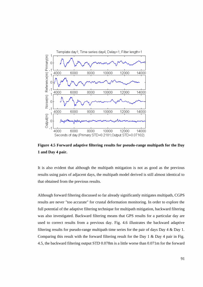
91


1 and Day 4 pair.

It is also evident that although the multipath mitigation is not as good as the previous

results using pairs of adjacent days, the multipath model derived is still almost identical to

that obtained from the previous results.

Although forward filtering discussed so far already significantly mitigates multipath, CGPS

results are never "too accurate" for crustal deformation monitoring. In order to explore the

full potential of the adaptive filtering technique for multipath mitigation, backward filtering

was also investigated. Backward filtering means that GPS results for a particular day are

used to correct results from a previous day. Fig. 4.6 illustrates the backward adaptive

filtering results for pseudo-range multipath time series for the pair of days Day 4 & Day 1.

Comparing this result with the forward filtering result for the Day 1 & Day 4 pair in Fig.

4.5, the backward filtering output STD 0.078m is a little worse than 0.071m for the forward

92

filtering case. Hence, a tentative conclusion is that forward correction is better than

backward correction.

Figure 4.6 Backward adaptive filtering results for pseudo-range multipath for the Day

4 and Day 1 pair.

Other combinations of pseudo-range multipath time series have also been calculated using

the adaptive filter. All of the results (including those not illustrated in the figures here) are

summarised in Table 4-1.

The standard deviations of the pseudo-range time series before multipath correction are

given in italics on the diagonal of the table. The standard deviations of the pseudo-range

time series after multipath correction using forward filtering are given in the triangle above

the diagonal while the backward filtering results are presented in the triangle below the

diagonal.

93

Table 4-1 Standard deviation of pseudo-range time series before (in italic) and after

multipath correction (unit: m).

Ref\Prim Day 1 Day 2 Day 3 Day 4 Day 1 0.229 0.046 0.059 0.071 Day 2 0.054 0.215 0.047 0.065 Day 3 0.068 0.048 0.211 0.052 Day 4 0.079 0.063 0.048 0.218

Considering these results, it can be concluded that:

• a pseudo-range multipath model can be reliably derived using an adaptive filter,

independent of the combinations of pseudo-range time series pairs used, as long as the

antenna environment remains unchanged;

• the older the reference signal, the less accurate the pseudo-range multipath correction;

• forward filtering is better than backward filtering; and

• the best pseudo-range multipath mitigation strategy is forward filtering using data on

two consecutive days (as indicated by the results in bold in Table 4-1), which reduces

the STD of the pseudo-range multipath time series to about one fourth.

4.4 Carrier-Phase Multipath Mitigation Using The Adaptive Filter

All the analyses in this section are based on Data set 2. Fig. 4.7 illustrates the forward

adaptive filtering results for carrier phase multipath for the Day 1 and Day 2 pair. From top

to bottom in the figure: the multipath time series of carrier phase results on Day 2, which is

used as primary input to the filter; the time series of Day 1, which is used as the reference

input to the filter; the carrier phase multipath model derived by the adaptive filter (noise);

and the output from the adaptive filter. Noted that its STD is only half of the primary input,

which indicates that the multipath effect has been reduced. The horizontal axis indicates the

seconds of the day and the unit of the vertical axis is millimetres.

94

Figure 4.7 Forward adaptive filtering results for carrier phase multipath for the Day

1 and Day 2 pair.

As in the case of the pseudo-range analyses described in Section 4.3, other combinations of

carrier phase multipath time series have also been calculated using the adaptive filter

described here. All of the results are summarised in Table 4-2.

The standard deviations of the carrier phase time series before multipath correction are

given in italics on the diagonal of the table. The standard deviations of the carrier phase

time series after multipath correction using forward filtering are given in the triangle above

the diagonal, while the backward filtering results are presented in the triangle below the

diagonal.

Table 4-2 Standard deviation of carrier phase time series before (in italic) and after

multipath correction (unit: mm).


95

Considering these results, it can be concluded that:

• a carrier phase multipath model can be reliably derived using an adaptive filter,

independent of the combinations of time series pairs used, as long as the antenna

environment remains unchanged;

• the older the reference signal, the less accurate the multipath correction to carrier phase;

• forward filtering is better than backward filtering; and

• the best carrier phase multipath mitigation strategy is forward filtering using data on

two consecutive days (as indicated by the results in bold in Table 4-2), which reduces

STD of the residual double-differenced time series to about one half.

4.5 Multipath Mitigation Using Adaptive Filtering Applied To CGPS Data

CGPS data in the RINEX format from the BRAN station in the SCIGN network for 4 days

beginning on 28 November 1999 (DOY 332) were used in this study of multipath

mitigation using an adaptive filter. An Ashtech Z12 GPS receiver was deployed at the

station. The data sampling interval is 30 seconds. The pseudo-range multipath time series

on L1 (Data set 3) over about 4 hours each day, for satellite PRN 2, were generated (Fig.

4.8), and then used in the adaptive filtering step (see Fig. 4.9, in layout similar to Fig. 4.1).

In this example, the multipath is reduced from 0.28m in the primary sequence to 0.15m in

the output.

96

Figure 4.8 Pseudo-range multipath for station BRAN of SCIGN (top to bottom plot:

DOY 332 to 335).


2 and Day 3 pair.

97

The adaptive filtering results are summarised in Table 4-3, arranged in the same format as

Tables 4-1 and 4-2. Conclusions similar to those in Section 4.3 can also be drawn, though

the STD in the output is only reduced to about half of the primary signal.

Table 4-3 Standard deviation of the pseudo-range time series before (in italic) and

after multipath correction (unit: m).


4.6 Implementing Procedures For Retro-Active Temporal Densification

There are three major steps in implementing an algorithm for multipath mitigation based on

adaptive filtering. The first step is to derive the necessary pseudo-range or carrier phase

multipath time series from GPS measurements. Since the pseudo-range "multipath

combination" (Eqs. (4.1) and (4.2)) is formed from one-way, dual-frequency phase and

pseudo-range data, which are available from a single GPS receiver, pseudo-range multipath

mitigation can be carried out on a single receiver basis.

In contrast, the carrier phase multipath series are obtained by double-differencing (Eq.

(4.4)) the phase measurements from two relatively closely-spaced receivers (close enough

to make the assumption of effective cancellation of spatially-correlated atmospheric

biases), one subject to multipath disturbance, and the other in a multipath-free environment.

This may become a limitation in a sparse CGPS array. However, in an array such as the

Japanese GEONET, it is always possible to identify some reference stations free of

multipath, and to generate the RINEX data for a Virtual Reference Station (VRS) located

close enough to the CGPS station targeted for multipath mitigation.

98

The second step is to input the derived multipath series into the adaptive filter to extract the

multipath model as was done in the studies reported in the previous sections. In the third

step, the multipath model (one-way pseudo-range, or double-differenced carrier phase) are

used to generate the multipath-corrected observable (pseudo-range or double-differenced

carrier phase) sequence, which can then be used for point positioning, baseline solutions,

etc.

4.7 Concluding Remarks

An adaptive filter based on the least-mean-square algorithm has been used to extract and

eliminate multipath. This algorithm can be used in real-time. The adaptive filter is a

powerful signal decomposer, able to distinguish the underlying coherent component of

multipath on consecutive days even though the pseudo-range and carrier phase data series

are significantly different. The extracted pseudo-range multipath behaves very much like

that of carrier phase, except that the variation is much larger (in the examples in this study,

it is two orders of magnitude larger).

Multipath models for both pseudo-range and carrier phase have been reliably derived using

the adaptive filter, independent of the combinations of time series pairs used, as long as the

antenna environment remains unchanged. However, it is found that the older the multipath

reference signal, the less accurate the multipath correction. Forward filtering is better than

backward filtering, and hence the best multipath mitigation strategy is forward filtering

using data on two consecutive days. Such a strategy reduces standard deviations of the

pseudo-range multipath time series to about one fourth the original values, and in the case

of carrier phase to about a half, based on the experimental GPS data considered here. In the

case of CGPS data from the SCIGN, the standard deviations of the pseudo-range multipath

time series is reduced to about a half. The results in Table 4-1 are much better than those in

Table 4-3 because the two antenna environments are very much different.

99

This multipath reduction technique can be used both on older data sets as well as new GPS

data, and because the technique uses pseudo-range and carrier phase data collected

simultaneously, it is sensitive to time-varying environmental effects at CGPS sites.

As a further study, GPS solutions with and without the multipath corrections can be

compared to assess improvements in precision and accuracy. The identification of

multipath reflectors at CGPS sites can be compared with site descriptions and changes in

environmental factors. Also, where possible, multipath-corrected solutions can be

compared with independent techniques such VLBI and SLR to test the effectiveness of this

retro-active temporal densification scheme.

In the next Chapter, the tools developed here to extract and mitigate multipath noise will be

used as a basis for using multipath effect as a signal.

100

As reviewed in Chapter 4, multipath has long been considered a major error source in

deformation monitoring using CGPS. In this Chapter, an attempt is made to use multipath

as a signal. As mentioned in Chapter 1.1, measurements from at least four GPS satellites

have to be used in order to solve for the three dimensional position of the GPS antenna and

the receiver clock. Using multipath as a signal to, e.g., monitor any change in the antenna

environment, it is proposed that each GPS satellite produce an independent result of the

monitoring of the environment, because multipath errors detected by the GPS receiver is

actually the outcome of interferometry between the direct and indirect GPS signals.

Because eight or more GPS satellites may be tracked from a single receiver, there are many

more measurements in the same epoch. Hence, this approach of using multipath as a signal,

according to Fig. 1.8, is in fact an all-GPS parallel temporal densification (Ge et al,

2000g). This scheme is aimed to take advantage of the GPS noise rather than pushing the

temporal limits of Fig. 1.7.

In this Chapter the procedures to extract multipath and to detect its change using the

adaptive filter are discussed in detail. Then the methodology is used to process CGPS data

from both a stationary and a changing antenna environment. Before concluding the

Chapter, mathematical models relating the multipath change to the change of the GPS

antenna environment, e.g. due to the movement of a slope, are derived, suggesting another

promising application of this all-GPS parallel temporal densification scheme.

This technique provides an easy-to-implement, quality assurance tool for CGPS antenna

environmental sensing after events such as typhoons, cyclones, snowfalls, volcano

5 ALL-GPS PARALLEL TEMPORAL DENSIFICATION – THE USE OF MULTIPATH EFFECTS AS A SIGNAL

101

eruptions, earthquakes, etc. Other possible applications include the monitoring of slope

stability and ground subsidence.

5.1 Introduction

No matter how well continuously operating GPS (CGPS) networks are designed, multipath

is a significant concern as it impacts on the quality of the CGPS outputs or 'products'.

Moreover, it may change slowly on a seasonal basis, or abruptly due to events such as a

snowfall.

Recently effort has also been made to make use of multipath, i.e. to use it as a signal rather

than a noise (e.g. Ding et al., 1999). The idea of analysing GPS errors and biases for signal

is not a new one. The best example is the so-called “GPS Meteorology”, which uses the

atmospheric refraction effects on GPS measurements as its input. Therefore, instead of

focusing on multipath mitigation, in this Chapter GPS multipath is used as a signal to sense

the change in the GPS antenna environment. This capability is very useful in the

maintenance and quality assurrance of CGPS networks such as the GEONET, where the

GPS monitoring environment can be changed not only by natural phenomenon such as

snow accummulation and tree growth, but also by disasters such as volcanic eruption,

typhoon and earthquake.

5.2 Multipath Extraction

Based on the analysis in Chapter 4, in the case of multipath extraction the multipath

residual sequence derived using the multipath combinations on a selected day can be

expressed as:

)()()( 111 tNtMPtD += (5.1)

where )(1 tN and )(1 tMP are the noise free of multipath and the noise contribution from

multipath respectively.

102

The multipath sequence on the next day is expressed as:

)()()( 222 tNtMPtD += (5.2)

where )(2 tN and )(2 tMP have similar definitions as )(1 tN and )(1 tMP .

According to previous studies (e.g. Han & Rizos, 1997), )(1 tMP and )(2 tMP are highly

correlated. But )(1 tN and )(2 tN are uncorrelated, which means that the two conditions of

using the adaptive filter as mentioned in Chapter 2 are only partly satisfied. In this case, as

demonstrated in a numerical simulation study in Chapter 2.4, the adaptive filter can still be

used to extract multipath from the combination results of the second day by employing

those of the first day as a reference signal. And )(2 tN and )(2 tMP will be outputs from the

filter as the “incoherent component” e(n) and “coherent component” y(n) respectively.

In order to extract multipath, M days worth of GPS data are divided into M-2 sets, each of

which consists of data from three consecutive days, as follows:

Set Consecutive days

1 1, 2, 3

2 2, 3, 4

3 3, 4, 5

…….

M-2 M-2, M-1, M

That is, there are 3 days in each set and among them there are 2 days overlapping in two

consecutive sets. After the multipath combination, following Eqs. (5.1) and (5.2) the

multipath residual sequences can be expressed as:

Day 1 in Set i, )()()( 111 tNtMPtD iii +=

103



Or for Day j in Set i, )()()( tNtMPtD ijijij +=

Where, i=1, 2, …, M-2

j=1, 2, and 3

We define @ as the adaptive filtering operator and A@B as the adaptive filtering process

using A as the primary input and B as the reference input. Then for the Day 1 and Day 2

pair:

)]()([)(@)( 2

^

2

^

12 tNtMPtDtD iiii = (5.3)

where )(2

^

tMP i is the adaptive filter estimated multipath for Day 2 in Set i (coherent output)

and )(2

^

tN i is the estimated receiver noise (incoherent output). Similarly for the Day 2 and

Day 3 pair:

)]()([)(@)( 3

^

3

^

23 tNtMPtDtD iiii =

The estimated multipath for Day j in Set i can be further expressed as:

)()()(^

tMPtMPtMP ijijij δ+= (5.4)

where )(2 tMP iδ is the multipath estimation error. If there is no change in the antenna

environment then:

)()( 1 ttMPtMP jiji ∆+= − (5.5)

104

t∆ is typically 236sec although it may be different for different satellites (Wanninger &

May, 2000).

5.3 Multipath Change Detection

If there is a change of the antenna environment between Days 2 and 3, then:

)()()( 23 tMPttMPtMP iii ∆+∆+= (5.6)

and

(5.7)

where )(tMPi∆ is the multipath change between Days 2 and 3 in Set i.

This approach to multipath change detection resembles the 3-pass differential radar

interferometry (InSAR) technique (Gabriel et al., 1989; also Chapter 7), in which the

elevation change is extracted by InSAR from the terrain model that is also constructed by

InSAR.

To summarize, as illustrated in Fig. 5.1, there are three main steps in implementing

multipath change detection based on adaptive filtering. The first step is to derive the

pseudo-range or carrier phase multipath residual time series through multipath combination

of the GPS measurements. Since the pseudo-range “multipath combination” is formed from

one-way, dual-frequency phase and pseudo-range data, which are available from the same

GPS receiver, pseudo-range multipath extraction can be implemented on a single receiver

basis.

)]()([)(@)( 22

^

3

^

tMPttMPtMPtMP iiii ∆∆+=

105

Multipathcombination

RINEX data

Multipath extraction

Multipath change detection

MPi1+Ni1

Day 1 in Set i

MPi2

MPi2+Ni2

Day 2 in Set i

DMPi2,3

MPi3

MPi3+Ni3

Day 3 in Set i

CGPS data

Figure 5.1 Multipath change detection procedures.

On the other hand, the carrier phase multipath series are obtained by double-differencing

the phase measurements from two relatively closely spaced receivers (close enough to

make the assumption of effective cancellation of spatially-correlated atmospheric biases),

one subject to multipath disturbance, and the other in a multipath-free environment. This

may be a severe limitation in a sparse CGPS array. However, in an array such as the

GEONET of Japan, it is always possible to identify some reference stations free of

multipath, and then generate the apparent RINEX data for a Virtual Reference Station

(VRS) (Bücherl et al., 2000) located close enough to the CGPS station considered for

multipath extraction.

In the second step, the adaptive filter (indicated by the star in Fig. 5.1) is used first to

extract the multipath from the residual series from two consecutive days, obtained from the

multipath combination (Eqs. (5.3) and (5.4)). Two multipath series will be obtained for

each 3 day set as a result.

In the third step, the adaptive filter is used again to detect the multipath change between the

two multipath series derived in the second step (Eq. (5.7).

In the following two sections this technique is first used for multipath change detection in a

stationary antenna environment to test if the detected change is zero when there is no

106

change in the antenna environment. Then it is applied for multipath change detection in a

changed antenna environment to test if the technique can identify the change when there is

indeed a change in the multipath disturbance caused by snowfall.

5.4 Multipath Change Detection in a Stationary Antenna Environment

Two data sets were used in this test, which were the same as those used in the Han & Rizos

(1997) study. In the first data set, the pseudo-range data over a period of nearly 3 hours for

four successive days, collected on the roof of the Geography and Surveying (GAS)

building, at the University of New South Wales (UNSW), from 30 September to 3 October

1997, using an Ashtech Z12 GPS receiver, were used to compute the pseudo-range

multipath time series. (In this study only the 'pseudo-range multipath time series' for L1 for

satellite PRN 9 are used.)

In the second data set, multipath series of double-differenced carrier phase measurements

over a period of nearly 2 hours on four successive days for two satellites (PRNs 1 and 21)

were calculated from data collected in an experiment carried out on the roof of the GAS

building at UNSW, from 28 April to 1 May 1997, using two Leica SR299 GPS receivers

with a baseline length of about 6 metres. Here the residual series of double-differenced

carrier phase observations are used as the 'carrier phase multipath time series' because they

reflect the multipath disturbance and observation noise (it is assumed that all the other

errors and biases are negligible because the baseline length is only of the order of 6 metres).

Fig. 5.2 shows the results of the pseudo-range multipath combination. From top to bottom

the plots represent the pseudo-range multipath residual sequences from Day 1 to Day 4. It

can be seen that although they look very similar there are differences between them due to

the change of uncorrelated noise from day to day. Also the t∆ (about 236sec) advance

between two consecutive days can be clearly seen.

107

Figure 5.2 Pseudo-range Multipath Combination Results.

Fig. 5.3 shows the multipath extraction result for Day 2 using the multipath residual

sequence of Day 1 as reference input. The extracted multipath on Day 2 (MP2) is displayed

in the third plot and the fourth one gives the uncorrelated noise. Similar extraction is done

on pairs of days: Day 2 & Day 3, and Day 3 & Day 4 so that MP2, MP3 and MP4 are all

obtained.

108

Figure 5.3 Multipath Extraction Result.

Figs. 5.4 and 5.5 display the multipath change detection results for pairs of days Day 2 &

Day 3 and Day 3 & Day 4. The multipath change is given in the fourth plot. Comparing the

plots for MP2, MP3, and MP4 in these figures, they look much more similar to each other

than the multipath residual sequences for Day 1 to Day 4, which highlights the importance

of multipath extraction for reliable multipath change detection.

109

Figure 5.4 Multipath Change Detection Result (Day 2-3).


110

Table 5-1 summarizes the standard deviations (STD) of the pseudo-range multipath

extraction (the first three rows) and change detection (the last two rows) results. Note that

in the multipath extraction step, the incoherent output is the uncorrelated noise and the

coherent output is multipath, while in the multipath change detection step the incoherent

output is the change of multipath and the coherent output is correlated multipath. Note that

the changes of multipath detected are not zero as they should be, but are 0.044 and 0.046m

in the pairs Day 2 & Day 3 and Day 3 & Day 4 respectively, which are nevertheless smaller

than the derived uncorrelated noise. Therefore, a tentative conclusion is that any multipath

change smaller than the uncorrelated noise (mainly the receiver noise) will go undetected.

Table 5-1 Multipath Extraction and Change Detection: Pseudo-Range Result.

Day IncoherentOutput STD

(m)

CoherentOutput STD

(m)2 0.046 0.2103 0.047 0.2054 0.052 0.212

2-3 0.044 0.2013-4 0.046 0.207

Now the technique is used to detect the multipath change of the carrier phase. Fig. 5.6

shows the results of the carrier phase multipath combination. From top to bottom the plots

represent the carrier phase multipath residual sequences from Day 1 to Day 4. As in the

case of pseudo-range, it can be seen that although they look very similar there are

differences between them due to the change of uncorrelated noise from day to day. Also the

t∆ (about 236sec) advance between two consecutive days can be clearly seen.

111

Figure 5.6 Carrier phase multipath combination result.

Fig. 5.7 shows the carrier phase multipath extraction result for Day 2 using the multipath

residual sequence of Day 1 as reference input. The extracted multipath on Day 2 (MP2) is

displayed in the third plot and the fourth one gives the uncorrelated noise. Similar

extraction is done on pairs of days: Day 2 & Day 3, and Day 3 & Day 4 so that MP2, MP3

and MP4 are all obtained.

112

Figure 5.7 Multipath Extraction Result.

Figs. 5.8 and 5.9 display the carrier phase multipath change detection results for pairs of

days Day 2 & Day 3 and Day 3 & Day 4. The multipath change is given in the fourth plot.

Comparing the plots for MP2, MP3, and MP4 in these figures, they look much more similar

to each other than the multipath residual sequences for Day 1 to Day 4, which highlights

the importance of carrier phase multipath extraction for reliable multipath change detection.

113



114

Table 5-2 summarizes the standard deviations (STD) of the carrier phase multipath

extraction (the first three rows) and change detection (the last two rows) results. Note that

in the multipath extraction step, the incoherent output is the uncorrelated noise and the

coherent output is multipath while in the multipath change detection step the incoherent

output is the change of multipath and the coherent output is correlated multipath. Note that

the changes of multipath detected are not zero as they should be, but are 0.966 and 1.010m

in the pairs Day 2 & Day 3 and Day 3 & Day 4 respectively, which are nevertheless smaller

than the derived uncorrelated noise. Therefore, a tentative conclusion, similar to the

pseudo-range case, is that any carrier phase multipath change smaller than the uncorrelated

noise (mainly the receiver phase noise) will go undetected.

Table 5-2 Carrier Phase Multipath Extraction and Change Detection Result.

Day IncoherentOutput STD

(mm)

CoherentOutput STD

(mm)2 1.543 2.3673 1.409 1.8664 1.457 1.969

2-3 0.966 1.6243-4 1.010 1.718

Therefore, one conclusion is that multipath change (either in pseudo-range or carrier phase)

above the receiver noise level (in the case of this study: code: 0.05m; phase: 1.5mm) could

be detected using this technique.

5.5 Multipath Change Detection in a Changed Antenna Environment

To test the capability of this technique in detecting multipath change, continuous GPS data

from two Japanese GEONET stations 960627 and 92110 located in the Tsukuba City were

used. In both Station 960627 and Station 92110, a Trimble 4000SSI receiver and a

Permanent L1/L2 antenna are installed at each station. The approximate coordinates X, Y

and Z for Station 960627 are -3957244.2254m, 3310369.6968m, and 3737538.8800m

(WGS84). Data from DOY 60 to 99 in the year 1998 are used in this test. While at Station

115

92110, the approximate coordinates X, Y and Z are -3957164.7499m, 3310202.7523m and

3737759.8264m. Data used are from DOY 60 to 88 in the year 1998 (unfortunately the

RINEX files for DOY 89 to 99 were corrupted when writing to a CD). Hence the distance

between the two stations is about 286m.

An abnormal change as large as 3cm in the time series of the baseline length between the

two stations was detected by Hatanaka & Fujisaku (1999). In their study, the elevation-

dependent antenna phase centre was compared for both L1 and L2, calculated every 3 hours

from 15:00 Japan Standard Time (JST) on March 5 (DOY 64) to 9:00 JST on March 6. A

big offset was seen in the result for the period 0:00 to 3:00 on March 6 compared to those

of the other segments, which corresponds to the time of a snowfall, as illustrated in Fig.

5.10. Moreover, the phase change on L2 was more significant that on L1.

Figure 5.10 Precipitation and temperature in Tsukuba from 5 March (DOY 64) to 6

March (DOY 65) 1998.

116

In order to test whether the adaptive filtering technique can detect this change in the

antenna environment, the CGPS data were processed following the procedures outlined in

the previous sections.

Fig. 5.11 is the pseudo-range multipath STD change on the C1 code at Station 960627 for

satellite PRN25. The total change (the biggest one in the figure) in the multipath STD from

DOY 64 to 65 is 0.19m, while the second biggest change is 0.10m from DOY 87 to 88,

which is an almost 100% increase.


PRN25.

Fig. 5.12 is the pseudo-range multipath STD change on the C1 code at Station 92110 for

satellite PRN 22. The total change (the biggest one in the figure) in the multipath STD from

DOY 64 to 65 is almost 0.09m, while the second biggest change is less than 0.07m from

DOY 72 to 73, which is not as significant as in Fig. 5.11. This might indicate that Station

92110 is less vulnerable to multipath.

117


PRN 22.

Figs. 5.13 and 5.14 are the results of carrier phase multipath change on L1 and L2

respectively in DD between Stations 92110 and 960627, for satellite pair PRNs 22 and 25.

In the two results, the biggest changes all occur on DOY 64 to 65, although the L2 result

gives a much better “signal-to-noise ratio”, which is in agreement with the result of

Hatanaka & Fujisaku (1999).

118


960627 for satellite pair PRNs 22 and 25.


960627 for satellite pair PRNs 22 and 25.

119

Therefore, it seems that when there is indeed a change in the antenna environment it will be

detected using this technique.

5.6 Slope Stability Monitoring Using Multipath Change

In this Section multipath has been used as a signal in a technique for slope stability

monitoring. The multipath combination, the multipath extraction and the detection of

multipath change are the same as described in previous sections. The change of multipath is

used in a least square process to estimate the slope movement parameters by employing the

mathematical models developed in this Section. The technique can also be used for

applications such as ground subsidence monitoring due to mining or underground water

extraction.

Traditional slope stability monitoring equipment and techniques include:

• Survey techniques (e.g., EDM and GPS leveling or photogrammetric surveys);

• Displacement monitoring pins and tape extensometers fixed across cracks or major rock

defects;

• Borehole inclinometers; and

• Extensometers anchored within the rock mass via boreholes drilled into slopes.

Compared to these techniques, there are obvious advantages in using the multipath effect

for slope stability monitoring. Multipath signals have common transmission time at the

satellite, almost common course through the atmosphere and are received by the same

receiver at the same time. Therefore, they are less noisy than the satellite-receiver double-

differenced observable. This ensures that the technique could achieve very high accuracy.

Other advantages include the movement of the slope at multiple reflecting points can be

monitored, which contributes to higher efficiency; moreover, the technique is relatively

cheap and highly automatic because a GPS receiver is a general purpose equipment

compared to the equipment used in some of the traditional techniques.

120

In this Section the mathematical models necessary to employ the GPS multipath effect for

slope stability monitoring are derived.

5.6.1 Models for relating multipath to slope movement

5.6.1.1 Two dimensional model for relating multipath to slope movement

Fig. 5.15 is a slope in the 2D illustration monitored by the GPS multipath. For the

application of slope stability monitoring using multipath effects, the antenna has to be

installed at the foot of the slope instead of on the slope itself. In the figure, α is the satellite

elevation angle, β is the incident angle of incoming GPS signal B’B on the slope, and the

slope is in angle θ to the ground. C’C is the direct line-of-sight signal from a GPS satellite

and RC is the reflected signal by the slope. The GPS antenna phase centre C is d metres

away from the foot of the slope and h metres above the ground DE. For the convenience of

calculation, AC is parallel to the ground DE, CB is perpendicular to RB and DF is

perpendicular to AC respectively.

d

h

D E

CA

R

B

αβ

θ

C’

B’

F

Figure 5.15 A slope in the 2D illustration monitored by the GPS multipath.

In ∆ ADF, DF = h and ∠ DAF = θ . Hence, AF = h / (tanθ ) and

121

AC = d + h / (tanθ ) (5.8)

In ∆ ACR, β = 1800 - (θ + α ) (5.9)

and ∠ CAR = 1800 - θ . Hence, CR / sin ( ∠ CAR) = AC / sin β or

CR = AC sin θ / sin β (5.10)

In ∆ CBR, ∠ CRB = 1800 - 2 β . Thus

BR = CR cos ( ∠ CRB) (5.11)

Therefore the geometric path length difference between the direct and reflected signals is: L

= BR + CR or by using Eqs. (5.8) to (5.11),

L = 2 sin (θ + α ) (d sin θ + h cos θ ) (5.12)

As will be seen from later discussions, Eq. (5.12) can be used to relate multipath to slope

movement.

5.6.1.2 Three dimensional model for relating multipath to slope movement

Fig. 5.16 is a slope in the 3D rectangular coordinate system monitored by the GPS

multipath. In the figure, the slope to be monitored is represented by a plane containing the

y-axis and point R. The slope is in angle θ to the horizontal plane xoy.ϕ is the orientation

of the slope. C’C is the direct line-of-sight signal from a GPS satellite and RC is the

reflected signal by the slope. The GPS antenna phase centre C is d metres away from the

foot of the slope and h metres above the ground DE. For the convenience of calculation, CB

is perpendicular to RB.

122

dh

OE

C

R

B

θ

C’

B’

R’

N

y

x

zϕ

γ

Figure 5.16 A slope in the 3D rectangular coordinate system.

Denoting the unit vectors along the x, y and z axes by →

i , →

j , and →

k , the direction vector of

the incident GPS signal is given by

γβα coscoscos'→→→→

−+= kjiBB (5.13)

where, α, β, and γ, which are linked to the satellite elevation angle and slope orientation ϕ

relative to north, can be calculated from the Keplerian elements of the GPS satellite and the

location of the antenna.

The normal to the reflecting surface is

→→→

+= kiRR θtan' (5.14)

The direction vector of the reflected ray is (Stavroudis, 1972)

→→→

+−= 'cos2' RRBBRC δ (5.15)

123

where δ is the incident angle and

cos δ = |'||'|

''→→

→→

⋅

•

RRBB

RRBB

= cosα sinθ – cosγ cosθ (5.16)

Since the coordinates of point C are (d, 0, h), the equation of the line R C is

x = d + (2 cosδ tanθ - cosα) v

y = (- cosβ) v (5.17)

z = h + (cosγ + 2 cosδ ) v

Where -∞ < v < ∞.

Since the equation of the slope surface is x tanθ + z = 0, the coordinates of reflecting point

R (xR, yR, zR) can be calculated using Eq. (5.17) by using v defined as

θδγθαθ

2cos/cos2costancos

tan

−−+

=dh

v (5.18)

With the coordinates of point R known, the length of RC is

RC = 222 )()( hzydx RRR −++− (5.19)

Therefore the geometric path length difference between the direct and reflected signals is

L = BR +RC = (1 + cos2δ) RC (5.20)

124

As will be seen from later discussions, Eq. (5.20) can be used to relate multipath to slope

movement.

5.6.2 The movement of slope and the change of geometric path length difference

between the direct and reflected signals

5.6.2.1 The 2D model

Eq. (5.12), the geometric path length difference between the direct and reflected signals is

L = 2 sin (θ + α ) (d sin θ + h cos θ ) (5.12)

By taking the partial derivative of L with respect to d and θ

∂ L / ∂ d = 2 sin (θ + α ) sin θ (5.21)

∂ L / ∂ θ = 2 d (sin 2θ cos α + sin α ) + 2 h cosα cos 2θ (5.22)

The relationship between the movement of slope and the change of geometric path length

difference between the direct and reflected signals can be expressed as

∆ L = ∆ d (∂ L / ∂ d)+ ∆ θ (∂ L / ∂ θ ) (5.23)

5.6.2.2 The 3D model

Eq. (5.20), the geometric path length difference between the direct and reflected signals is

L = (1 + cos2δ) RC (5.20)

By taking the partial derivative of L with respect to d and θ

125

∂ L / ∂ d = (1 + cos2δ) ( ∂ RC / ∂ d) (5.24)

∂ L / ∂ θ = (1 + cos2δ) ( ∂ RC / ∂ θ ) – 2 RC sin2δ (∂ δ / ∂ θ ) (5.25)

Using Eqs. (5.16) to (5.19)

∂ RC / ∂ d = RCd

zhz

d

yy

d

xdx R

RR

RR

R /])()1)([(∂∂

−+∂∂

+−∂∂

−

∂ RC / ∂ θ = RCz

hzy

yx

dx RR

RR

RR /])()[(

θθθ ∂∂

−+∂∂

+∂∂

−

∂ δ / ∂ θ = cosα cosθ + cosγ sinθ

where

∂ xR / ∂ d = 1 + (2 cosδ tanθ - cosα) (∂ v/ ∂ d)

∂ yR / ∂ d = (- cosβ) ( ∂ v/ ∂ d)

∂ zR / ∂ d = (cosγ + 2 cosδ ) ( ∂ v/ ∂ d)

∂ xR / ∂ θ = (2 cosδ tanθ - cosα) ( ∂ v/ ∂ θ) - 2 v sinδ tanθ ( ∂ δ / ∂ θ) + 2 v cosδ / cos2θ

∂ yR / ∂ θ = (- cosβ) ( ∂ v/ ∂ θ)

∂ zR / ∂ θ = (cosγ + 2 cosδ ) ( ∂ v/ ∂ θ) – 2 v sinδ ( ∂ δ / ∂ θ)

∂ v/ ∂ d = θδγθα

θ2cos/cos2costancos

tan

−−

∂ v/ ∂ θ θ

θδθαθθ 3cos

)sincos2cos(coscos

tan

+−⋅

+=

vd

dh

v

126

Therefore, just as in the case of 2D model, the relationship of the 3D model between the

movement of slope and the change of geometric path length difference (between the direct

and reflected signals) can be expressed using Eq. (5.23).

5.6.3 The change of multipath and the movement of slope

The effect of multipath is characterized by four parameters (all of which are relative to the

direct signal): 1) amplitude; 2) time delay; 3) phase; and 4) phase rate of change. For this

analysis only 1) and 3) are significant.

Now consider first the case in which only one reflected signal from a planar surface

interferes with the direct line-of-sight carrier signal. The direct and the reflected signals can

be expressed as

)cos(

cos

1

0

ppp

p

AS

AS

θϕα

ϕ

+=

= (5.26)

where, S0 is the direct signal from the satellite and S1 is the reflected signal from the surface;

A and ϕ p are the amplitude and the phase of the signal, respectively; α p is the amplitude

reduction factor which fulfills the inequality 0<α p<1; θ p is the phase shift caused by

multipath. To avoid confusion of notations with the previous discussions, a “p” in

superscript is used to denote variables specific to multipath once inside the receiver.

Suppose the geometric path length difference between the direct and reflected signals is L

and the microwave refractive index at the antenna site is n. L can be linked to slope

parameters using Eqs. (5.12) (the 2D model) or (5.20) (the 3D model). The phase shift can

be written in radians as

λπ

θnLp 2

= (5.27)

127

where λ is the length of the code (pseudo-range) or wavelength (carrier phase) of the signal.

When the two signals interfere at the antenna centre, the composite signal is (e.g., Leick,

1995)

)cos('10ppASSS ψϕ +=+= (5.28)

where the resultant amplitude A' is

2/12 ))(cos21(' pppAA αθα ++= (5.29)

and the phase delay ψ p is

+

= −pp

ppp

θαθα

ψcos1

sintan 1 (5.30)

For the planar surface, the multipath error can be found by

λπ

ψ2

p

MP = (5.31)

Because in Eq. (5.30) both θ p and 2Nπ + θ p (N is an integer) will give the same ψ p, there

is a problem with the integer ambiguity N when trying to link multipath MP with L using

Eqs. (5.31), (5.30) and (5.27). To address this problem, Eq. (5.27) is rewritten as

λπ

πθnL

Np 22 =+ (5.27a)

128

Suppose there is still another planar surface to reflect the GPS signals, and the reflected

signal is

)cos( 112ppp AS θϕα += (5.32)

By introducing, ppnew

p ψϕϕ += ; ppnew

p ψθθ −= 1 ; and

2/121 ))(cos21/( pppp

newp αθααα ++=

Eqs. (5.26) and (5.32) can be re-written as

)cos('

cos'

2 newp

newp

newp

newp

AS

AS

θϕα

ϕ

+=

= (5.33)

Hence, the new composite signal can be written as

)cos(')( 210210 mp

newp

mm ASSSSSSS ψϕ +=++=++= (5.34)

where mA' and mpψ can be calculated using equations similar to Eqs. (5.29) and (5.30).

Therefore, an “equivalent ideal slope” with planar surface can always be found for the

practical slopes which can reflect the GPS satellite signals to the antenna from multiple

points. The following discussion on the single reflected signal case are equally valid for the

multiple reflected signal case.

To avoid the integer ambiguity as describe in Eq. (5.27a), the change of multipath rather

than the multipath itself is used to estimate the slope movement. The change of multipath

can be expressed as

∆ MP = ∆ d • (∂ MP / ∂ d)+ ∆ θ • (∂ MP / ∂ θ )

129

= ∆ d • PMP d+ ∆ θ • PMP θ (5.35)

where

PMP d = ∂ MP / ∂ d = d

L

dL

d

d

d

d

dMP p

p

p

p ∂∂

⋅⋅⋅θ

θψ

ψ (5.36)

PMP θ= ∂ MP / ∂ θ =θ

θθψ

ψ ∂∂

⋅⋅⋅L

dL

d

d

d

d

dMP p

p

p

p (5.37)

From Eqs. (5.31), (5.30) and (5.27a)

λπθ

θααθαα

θψ

πλ

ψ

n

dL

d

d

d

d

dMP

p

ppp

ppp

p

p

p

2

cos2)(1

cos)(

2

2

2

=

+++

=

=

(5.38)

∂ L / ∂ d and ∂ L / ∂ θ are calculated using Eqs. (5.21) and (5.22) (for 2D model) or (5.24)

and (5.25) (for 3D model). Note also that the integer ambiguity is not present in Eq. (5.38),

which indicates that ambiguity resolution has been avoided by using the change of

multipath rather than the multipath itself.

Considering that MP, α , θ and d are all changing with respect to time t due to the

movement of the slope, and satellite and MP and α are different for different satellites, Eq.

(5.35) can be re-written as

∆ MPi(t) = ∆ d(t) ( ∂ MP i(t) / ∂ d(t))+ ∆ θ (t) ( ∂ MP i(t) / ∂ θ (t)) (5.39)

where i stands for the PRN of the satellite. For the convenience of later discussions, let

130

PMPdi(t) = ∂ MP i(t) / ∂ d(t) (5.40)

PMPθi (t) = ∂ MP i(t) / ∂ θ (t) (5.41)

Then Eq. (5.39) can be further re-written as

∆ MPi(t) = ∆ d(t) • PMPdi(t) + ∆ θ (t) • PMPθ

i (t) (5.39a)

Hence, using this equation the change of multipath ∆ MPi(t) can be related to the

movement of slope ∆ d(t) and ∆ θ (t). Note that if θ is held as zero, this technique can

also be used for applications such as ground subsidence monitoring due to mining or

underground water extraction.

5.6.4 Least square estimation of slope movement using the change of multipath

Because there are at least four GPS satellites (even more than eight if low-elevation angle

ones are also considered) in the field of view of an antenna anywhere on the Earth, but

there are only two variables of slope movement to be estimated, there are many redundant

measurements (a result of all-GPS parallel temporal densification!). Consider the vector of

unknowns or the slope movement vector

X = [ ∆ d(t) ∆ θ (t)]T (5.42)

Hence, least square estimation is introduced into the data analysis. Denote the observation

vector which consists of the change of both pseudo-range ( ∆ MPi(t)) and carrier phase ( ∆

MPphi(t)) multipath calculated by Eq. (5.39a) for satellites PRN1 to PRNi all available at

time t as

131

L = [ ∆ MPPRN1(t) ∆ MPPRN2(t) … ∆ MPPRNi(t)

∆ MPphPRN1(t) ∆ MPphPRN2(t) … ∆ MPphPRNi(t)]T (5.43)

Then the coefficient matrix can be determined using Eqs. (5.40) and (5.41)

B =

(t)PMP (t)PMP

....

(t)PMP (t)PMP

(t)PMP (t)PMP

(t)PMP (t)PMP

....

(t)PMP (t)PMP

(t)PMP (t)PMP

PRNiphPRNid

ph

PRN2phPRN2d

ph

PRN1phPRN1d

ph

PRNiPRNid

PRN2PRN2d

PRN1PRN1d

θ

θ

θ

θ

θ

θ

(5.44)

Assume the vector of observation errors is ∆ , then the observation equation is

L = B X + ∆ (5.45)

Therefore, the least square estimation of the slope movement is (Giordano & Hsu, 1985)

^

X = (BT P B)-1 BT P L (5.46)

where P = D1−

∆ and D∆ is the variance matrix of ∆ .


The all-GPS parallel temporal densification scheme is proposed for the detection of

multipath change as a signal at permanent GPS stations based on an adaptive filter using

the least-mean-square algorithm. The technique was tested on some experimental data,

132

indicating that the multipath change above the receiver noise level can be detected. A

further test was done with some CGPS data from the Japanese GEONET when there was a

snowfall. The results indicate that if there is a change in the antenna environment the

proposed technique will indeed detect it in both the pseudo-range and carrier phase data.

For applications of pseudo-range multipath change detection, data from a single dual-

frequency receiver is sufficient. For applications of carrier phase multipath change

detection, data from two closely-spaced receivers have to be used. This may become a

limitation in a sparse CGPS array. However, in an array such as the GEONET it is always

possible to identify some reference stations free of multipath, and to generate the RINEX

data for a Virtual Reference Station located close to the CGPS station targeted for multipath

change detection. For reliable multipath change detection, the temporal resolution of this

method is 24 hours.

As an application of the technique, the mathematical models for slope stability monitoring

using the change of GPS multipath effects have been given in this Chapter. It is found that

an “equivalent ideal slope” with planar surface can always be found for the practical

slopes which can reflect the GPS satellite signals to the antenna from multiple points.

Moreover, ambiguity resolution has been avoided by using the change of multipath rather

than the multipath itself in the monitoring of slope movement. The change of multipath is

used in a least square process to estimate the slope movement parameters by employing the

mathematical models developed. The system is designed to function as an early warning

system through monitoring the sliding precursors. When the sliding is imminent, the system

has to be withdrawn.

This all-GPS parallel temporal densification scheme provides an easy-to-implement quality

assurrance tool for CGPS antenna environment sensing after disasters such as typhoons,

cyclones, and earthquakes. Other possible applications include the monitoring of slope

stability and ground subsidence.

133

In recent years space geodetic techniques such as the Global Positioning System (GPS),

Very Long Baseline Interferometry (VLBI), and Satellite Laser Ranging (SLR) have been

collocated to address many applications in geoscience. Cross-technique parallel temporal

densification requires the integration of the continuous GPS (CGPS) results with VLBI and

SLR data. In other words, an appropriate fusion of these multi-technique space geodetic

results must be developed. VLBI measures the difference between the arrival times, at two

Earth-based antennas, of a radio wavefront emitted by a distant quasar. SLR measures the

round-trip-time of travel of a signal between a ground-based laser transmitter/receiver and a

satellite equipped with optical corner reflectors. Whilst results from all these techniques are

contaminated by various biases and errors, when GPS, VLBI and SLR instruments are

installed at the same site, the same crustal displacement signature will be present as a

common-mode signal. The results can therefore be fused, GPS-VLBI and GPS-SLR, using

the adaptive filtering approach based on the Least-Mean-Square algorithm described in

Chapter 2, or by extending the adaptive filter to a three input (one primary, two references)

and two output system (Ge et al, 2000b). The GPS-VLBI and GPS-SLR outputs can be

used to verify each other as well.

In this Chapter, data from the Matera Station in Italy and the Wettzell Station in Germany

have been used to test this densification scheme.

6.1 Introduction

The space geodetic techniques of GPS, VLBI, and SLR have been used to address

applications such as the monitoring of plate and polar motion of the Earth. In recent years,

6 CROSS-TECHNIQUE PARALLEL TEMPORAL DENSIFICATION – THE INTEGRATION OF GPS WITH VLBI

AND SLR

134

GPS, VLBI and SLR instruments have been collocated for the purpose of monitoring active

fault movement in campaigns such as the Key Stone Project (KSP) of Japan. In 1999 the

common-mode signal from the GPS, VLBI and SLR techniques, extracted from the

published KSP results (Takahashi & Ichikawa, 1999), was analysed using the proposed

methodology. This methodology has also been validated by researchers from M.I.T.

(Herring, 1999).

In the case of GPS measurements, the biases and errors include ephemeris uncertainties,

satellite clock errors, selective availability effects (before 1 May 2000), receiver clock

errors, reference station coordinate uncertainties, ionospheric delay, tropospheric delay,

carrier phase ambiguity, unmodelled residual biases, carrier phase cycle slips, multipath

disturbance, antenna phase centre offset, and random observation error. In the case of the

VLBI measurements, the biases and errors may include the effects of temperature

variations on the hydrogen maser, the ionosphere, the wet component of the troposphere,

the structure of the radio sources used in the observations, and so on. In the case of SLR

measurements, the biases and errors may include the effects of the satellite ephemeris

uncertainties, the precession and nutation uncertainties, satellite libration theory, elastic

deformations of the Earth surface, atmospheric retardation of photons and the behavior of

terrestrial clocks. Despite the fact that, for example, dual-frequency data can be used to

negate the effect of the ionosphere, and water vapour radiometers can be used for wet

tropospheric calibration, many of these biases and errors contaminate the final GPS, VLBI

and SLR results.

In Section 2 of this Chapter, detailed analyses and intercomparisons of the biases and errors

in the GPS, VLBI and SLR results are presented. The decorrelation among the baises and

errors makes it feasible to extract the crustal movement as the common-mode signal from

collocated GPS, VLBI and SLR results.

In Section 3 of this Chapter, the common-mode signals from the results of collocated GPS,

VLBI and SLR at Matera (Italy) and Wettzell (Germany), extracted using an adaptive filter

based on the Least-Mean-Square algorithm, are presented.

135

6.2 Analyses And Comparisons of The Biases And Errors In The GPS, VLBI And SLR

Results

In the case of GPS, VLBI and SLR results, the time series for a station can be expressed as:

)()()()( nxnxnsnd incoco ++= (6.1)

)(')(')(')(' nxnxnsnr incoco ++= (6.2)

)(")(")(")(" nxnxnsnr incoco ++= (6.3)

where s(n), s‘(n), and s“(n) are the signals free of noise (true crustal movement) detected

by GPS, VLBI, and SLR respectively; and )(nxco and )(nxinco are the contributions to GPS

results from noises and biases which are coherent and incoherent, respectively, with those

in VLBI and SLR results. )(' nx co and )(' nx inco and )(" nx co and )(" nx inco are analoguous

to )(nxco and )(nxinco . As a result, )()( nxns co+ will behave as the common-mode signal

amongst the GPS, VLBI and SLR results.

In this case, can the adaptive filter be used to extract the true crustal movement s(n) from

the GPS result d(n) by employing the VLBI result r‘(n) and/or SLR result r“(n) as

reference signals? As discussed in Chapter 2.4, and also in Ge (1999), there are two special

cases to be considered in the application of an adaptive filter. Eq. (6.1) can be treated as a

linear combination of the two cases. Therefore, by decorrelating the noises and biases in

collated GPS, VLBI and SLR results theoretically it is possible to obtain the true crustal

movement s(n) by using GPS, VLBI and SLR results as inputs to an adaptive filter. Hence,

the success of the cross-technique parallel temporal densification scheme in integrating

collocated GPS, VLBI, and SLR results using the adaptive filter depends on the

decorrelation among the noises and biases in the results, i.e. xco (n) → 0 in Eq. (6.1).

136

In GPS measurements, the biases and errors include satellite ephemeris uncertainties,

satellite clock errors, selective availability effects, receiver clock errors, reference station

coordinate uncertainties, ionospheric delay, tropospheric delay, carrier phase ambiguity,

unmodelled residual biases, carrier phase cycle slips, multipath disturbance, antenna phase

centre offset, and random observation error (Rizos, 1996).

The satellite ephemeris uncertainties (bias) is the discrepancy between the true position

(and velocity) of a satellite and its known value. In the Broadcast Ephemerides within the

GPS Navigation Message, the bias can range from (usually) less then 10m to (very rarely)

up to 100m. In the post-processed ephemerides the bias is well below the metre level.

The satellite clock errors consist of the offset, drift and drift-rate of the satellite clocks with

respect to GPS Time. These errors are modelled to an accuracy of about 20 nanoseconds.

Selective Availability (SA) is a further artificial dithering of the satellite clocks causing

several dekametres error in the range (or phase-range equivalent). Fortunately SA has been

switched off since 1 May 2000.

The receiver clock errors due to the use of quartz crystal oscillators in GPS receivers

include the error in defining the time origin (tying the clock to a well established time scale,

such as GPS Time, to the 0.01 microsecond level with SA off) and the clock drift.

The reference station coordinate uncertainties in differential GPS positioning (essential for

overcoming the satellite dependent biases described above) will cause a bias in the solution

because the coordinates of the reference station are held fixed during data processing.

Hence, in effect, only the relative position (or baseline components) relating the second

receiver to the first (reference) receiver are estimated.

In terms of the atmospheric effects, the ionospheric and tropospheric delays will affect both

pseudo-range and carrier phase measurements. However, the dispersive nature of the

ionosphere can be used in actually removing most of the ionospheric delay effect by

making pseudo-range and/or carrier phase measurements on both L-band frequencies, and

137

forming the "ionosphere-free" combination. In the case of the tropospheric delay bias, 90%

due to the dry atmosphere can be modelled very well, while 10% due to the wet component

of the atmosphere is difficult to account for.

The ambiguity and cycle slips are specific to the carrier phase observable, and hence are

relevant to GPS only.

The unmodelled residual biases remaining after the appropriate differencing of phase data,

collected simultaneously by two GPS receivers, are primarily due to the:

• differential ionospheric refraction between the two sites (if not eliminated by the

"ionosphere-free" combination);

• differential tropospheric refraction between the two sites; and

• second-order effect of orbit error on the baseline solution.

The multipath disturbance is caused by extraneous reflections of GPS signals from nearby

metallic objects, ground or water surfaces reaching the antenna. Whilst both on-the-receiver

and post-processing techniques have been used to mitigate the multipath effects as

reviewed in Chapter 4, the disturbance is still common in the final GPS result.

The antenna phase centre offset is the distance between the physical and the electrical

centres of the antenna. Because the electrical centre varies with the direction and strength

of the incoming signal, a variation in the satellite-receiver geometry will cause the position

of the electrical centre to also vary, which introduces errors into the GPS result.

The random observation error for GPS is typically at the millimetre level.

In VLBI measurements, the biases and errors may include the effects of temperature

variations on the hydrogen maser, the ionosphere, the wet component of the troposphere,

the structure of the radio sources used in the observations, and so on. Measuring the

difference between the arrival times at two or more Earth-based antennas of the radio

wavefronts, at S-, X- and sometimes K-bands (Takashima et al, 2000), emitted by many

138

distant quasars, VLBI is free of the satellite-dependant biases and errors. Instead, the

structure of the radio sources used in the observations will introduce some errors, which are

of course very unlikely to be correlated to the satellite-dependant biases and errors in the

GPS result.

However, when the radio signals from these quasars travel through the atmosphere, biases

correlated to the ionospheric and tropospheric biases in GPS result will be introduced

because the S- (f=2100-2450MHz, λ≈15cm), X- (f=8100-9000MHz, λ≈3cm) and K- (f=

19500-25000 MHz, λ≈1.5cm) bands used by VLBI as well as the L-band (fL1=

1575.42MHz, λL1≈19cm; fL2=1227.60MHz, λL2≈24cm) used by GPS are all in the

microwave band. For example, the ionospheric group delay d ion and the ionospheric phase

delay φion for a microwave propagating from a quasar or GPS satellite to the ground is

approximated by (Rizos, 1996):

dion = −φion

c

f

≈ 40.28 ⋅STEC

f 2

≈ 40.28cosecζ

⋅VTEC

f 2

(6.4)

where:

d ion is the ionospheric group delay in units of metres;

φ ion is the ionospheric phase delay in units of cycles;

c is the speed of electronic magnetic radiation in a vacuum (m/sec);

cosec ζ is the cosecant of the zenith angle of the line-of-sight to the microwave source;

f is the signal frequency (Hz);

STEC is the Slant Total Electron Content, expressed as the number of free electrons per

square metre (el/m2); and

VTEC is the Vertical Total Electron Content (zenith direction) (el/m2).

139

Note, from Eq. (6.4), the higher the frequency, the smaller the ionospheric delay effect. Let

us assume that VTEC is 10^18 electrons per square meter. This is a high but not unrealistic

value. Then the contribution at GPS L band frequencies is of the order of 1 for

VTEC/(f**2). It is only marginally greater than 10mm at the top end of X band and is

negligible for optical wavelengths. Note that at K band frequencies the VLBI contribution

is only 1.6mm. Thus the ionosphere impacts differently upon the three techniques.

In addition, the tropospheric water vapour leads to correlations between VLBI and GPS

observations.

The effects of temperature variations on the hydrogen maser on the VLBI result are

analogous to the receiver clock errors in the GPS result. But correlation between them is

expected to be low since different types of clock are used in VLBI and GPS.

Since a VLBI antenna is quite unidirectional due to it's large diameter, there shouldn't be

any multipath effect in VLBI observations.

In the case of SLR measurements, the biases and errors may include the effects of the

satellite ephemeris uncertainties, the precession and nutation uncertainties, satellite

libration theory, elastic deformations of the Earth surface, atmospheric retardation of

photons and the behavior of terrestrial clocks. Among them, the effects of the satellite

ephemeris uncertainties will be a correlated error between GPS and SLR if a GPS satellite

is used as a SLR target as well. As a matter of fact, optical corner reflectors have been

installed on two of the GPS satellites. Fortunately, they do not normally contribute to a

SLR solution which is usually restricted to LAGEOS type satellites. Again the atmospheric

biases will contaminate the SLR result but would not correlate with those in GPS as

strongly as in the case of VLBI because the wavelength of the laser pulse used in SLR is

usually at 532nm, which is in the visible light band, rather than the microwave band.

140

Table 6-1 summarizes the above discussion and indicates the degree of decorrelation of

GPS noises and biases in various combinations with VLBI and SLR. From the table, it can

be concluded that noises and biases in GPS result can be significantly reduced by

integrating with collocated VLBI and SLR results, which makes the cross-technique

parallel temporal densification scheme feasible.

Table 6-1 Decorrelation of GPS noises and biases in various combinations with VLBI

and SLR.

Combinations

Noises and biases

GPS- VLBI

GPS- SLR

GPS- VLBI -SLR

satellite ephemeris uncertainties

0

0.5

0 satellite clock errors

0

0

0 Selective availability effects

0

0

0 receiver clock errors

0

0

0 Ref. station coordinate uncertainties

0

0

0 ionospheric delay

1

0

0 tropospheric delay

1

0.5

0.5 carrier phase ambiguity

0

0

0 carrier phase cycle slips

0

0

0 multipath disturbance

0

0

0 antenna phase centre offset

0

0

0 Random observation error

0

0

0

Remarks: 0 uncorrelated;

0.5 partially correlated; and

1 correlated.

141

6.3 The Integration of Collocated GPS, VLBI And SLR Results

In this section, data from two stations Matera and Wettzell are used in the integration of

collocated GPS, VLBI and SLR results using the adaptive filter.

Details of the two stations are summarized in Table 6-2. From the table the distances from

the VLBI Monument to the GPS Mark and from the SLR Monument to the GPS Mark are

58.000m and 38.334m respectively at Matera Station. Hence, an absolute collocation is not

possible. Even for the collocated GPS and GLONASS (and in the future Gelileo) which

share the same antenna, there is the problem of phase centre differences. Therefore, it is

important to ensure that the distances between the marks are so small that they will not lead

to the decorrelation of s(n), s‘(n), and s“(n) in Eqs. (6.1) to (6.3).

142

Table 6-2 Details of the Matera and Wettzell stations

Station MATERA WETTZELL City or Town Matera Koetzting

State or Province Basilicata Bavaria Country Italy Germany

Tectonic Plate Adriatic-African Eurasian

Parent/Funding organization

Agenzia Spaziale Italiana (Asi), Italy

Bundesamt fuer Kartographie und Geodasie (BKG) Forschungseinrichtung Satellitengeodaesie der Technischen Universitaet Muenchen (FESG)

Collocated space geodetic techniques

GPS SLR VLBI PRARE*

GPS SLR VLBI PRARE GLONASS

Other

collocated techniques

Gravimeter (super conducting) seismometer time & frequency laboratory meteorological sensors water vapour radiometer

GPS

Monument Inscription: Stable pillar on the roof

Approximate Position (m): X: 4641949.709 Y: 1393045.298 Z: 4133287.333 Latitude (deg): 40.6491 N Longitude (deg): 16.7044E Elevation (m): 535.65 GPS Receiver: TRIMBLE 4000SSI GPS Antenna: Trimble L1/L2 Dorne Margolin element with Choke-rings

Monument Inscription: Pillar Approximate Position (m): X: 4075580.695 Y: 931853.668 Z: 4801568.036 Latitude (deg): 49.144197129 N Longitude (deg): 12.878907601 E Elevation (m): 666.024 GPS Receiver: AOA SNR-8000 ACT GPS Antenna: AOAD/M_T

VLBI

Rack: Mark IIIA Recorder: VLBA Hydrogen-maser model: OSCILLOQUARTZ EFOS-8 Other frequency standards: 2 CESIUM (HP 5061) GPS timing receiver model: FTS-8400 X/S receiver RF bandwidths:

2210-2450 8180-8980 MHz Differential Components from VLBI Monument to GPS Mark dx (m): -10.946 dy (m): -42.246 dz (m): 38.203 Accuracy (mm):6 Date Measured: 01-NOV-1991

Rack: Mark IIIA Recorder: Mark IIIA Hydrogen-maser model: EFOS-1, EFOS-3, and EFOS-13 Other frequency standards: HP Cesium standard GPS timing receiver model: ALLAN OSBORNE TTR-6 X/S receiver RF bandwidths: 8100-9000 MHz, 2100-2300 MHz Differential Components from VLBI Monument to GPS Mark dx (m): -40.802 dy (m): -118.398 dz (m): +61.317 Accuracy (mm): 1

Date Measured: 13-FEB-1995

Station configura-

tions

SLR

Instrument: permanent Differential Components from SLR Monument to GPS Mark dx (m): 15.172 dy (m): 24.826 dz (m): -24.959 Accuracy (mm):2 Date Measured: JUL-1996

Instrument: permanent Differential Components from SLR Monument to GPS Mark dx (m): -3.828 dy (m): -68.200 dz (m): +15.517 Accuracy (mm): 1

Date Measured: 13-FEB-1995

* PRARE (the Precision RAnge and Range-rate Experiment)

143

In order to integrate the collocated results of GPS, VLBI and SLR, two configurations can

be designed for the adaptive filter: a two-input-and-two-output, and a three-input-and-two-

output. In the two-input-and-two-output configuration, the inputs consist of a primary input

(GPS result) and a reference input (VLBI or SLR result) and the outputs consist of the

common-mode signal between the primary and reference inputs and the uncorrelated

component in the primary signal. This configuration enables the comparison between the

common-mode signals derived from GPS-VLBI and GPS-SLR combinations. In the three-

input-and-two-output configuration, the inputs consist of a primary input (GPS result) and

two reference inputs (VLBI and SLR results) and the outputs consist of the common-mode

signal among the primary and the two reference inputs and the uncorrelated component in

the primary signal. This configuration enables the extraction of the common-mode signal

by the integration of collocated GPS, VLBI and SLR results.

In the GPS-VLBI combination, the overlap period of GPS and VLBI results for Matera is

from 25 May 1992 to 1 May 1999, and for Wettzell from 9 January 1996 to 22 July 1998.

Coordinates for the two stations were estimated on a daily and fortnightly basis using GPS

and VLBI data respectively, resulting in two time series for each station. The GPS time

series are given in ellipsoidal coordinates while the VLBI results are in Cartesian

coordinates. Hence, the VLBI time series were converted to ellipsoidal coordinates before

being used in the filtering.

Fig. 6.1 is the integration of GPS and VLBI at Matera for the longitude component. From

top to bottom the plots are: the GPS time sequence as primary input; the VLBI time

sequence as reference input; extracted common-mode signal as coherent output; and the

incoherent output from the adaptive filtering system. In all these plots, the horizontal axis

indicates year and the vertical axis the longitude change in centimetres. The blue (black)

curves are the respective data while the red (or grey) straight lines in the first three plot are

the least-squares fits of the data, so that the rate of movement in the stations and the

repeatability of the results can be estimated. It can be seen that the repeatability of the

derived common-mode signal (0.46cm) is better than that of GPS (0.59cm) and that of

144

VLBI (0.62cm) and perhaps 2.38cm/yr is a more realistic estimate for the rate of plate

movement (further study is needed to compare these results with the NUVEL-1 Model,

DeMets et al., 1990).

Calculations on other components for station Matera and all three components for station

Wettzell were also done (Figs. 6.2 to 6.6), and the results were summarized in Table 6-3. In

the table, mLatitude, mLongitude and mHeight stand for the three components of the

Matera Station while wLatitude, wLongitude and wHeight are those of the Wettzell Station.

Conclusions similar to that for the longitude component of Matera can be made for the

other results in the table. The differences between GPS and VLBI results in this study and

the JPL (the Jet Propulsion Laboratory) GPS and GSFC (the Goddard Space Flight Center)

VLBI (Ma & Ryan, 1998) results are due to the data length used in the estimations. For

example, data from 16 November 1983 to 22 July 1998 were used in the GSFC VLBI

estimation for Wettzell, whilst in this study only data from 9 January 1996 to 22 July 1998

were used, due to the availability of collocated GPS result.

145

Figure 6.1 Integration of GPS and VLBI at Matera: the longitude component.

Figure 6.2 Integration of GPS and VLBI at Matera: the latitude component.

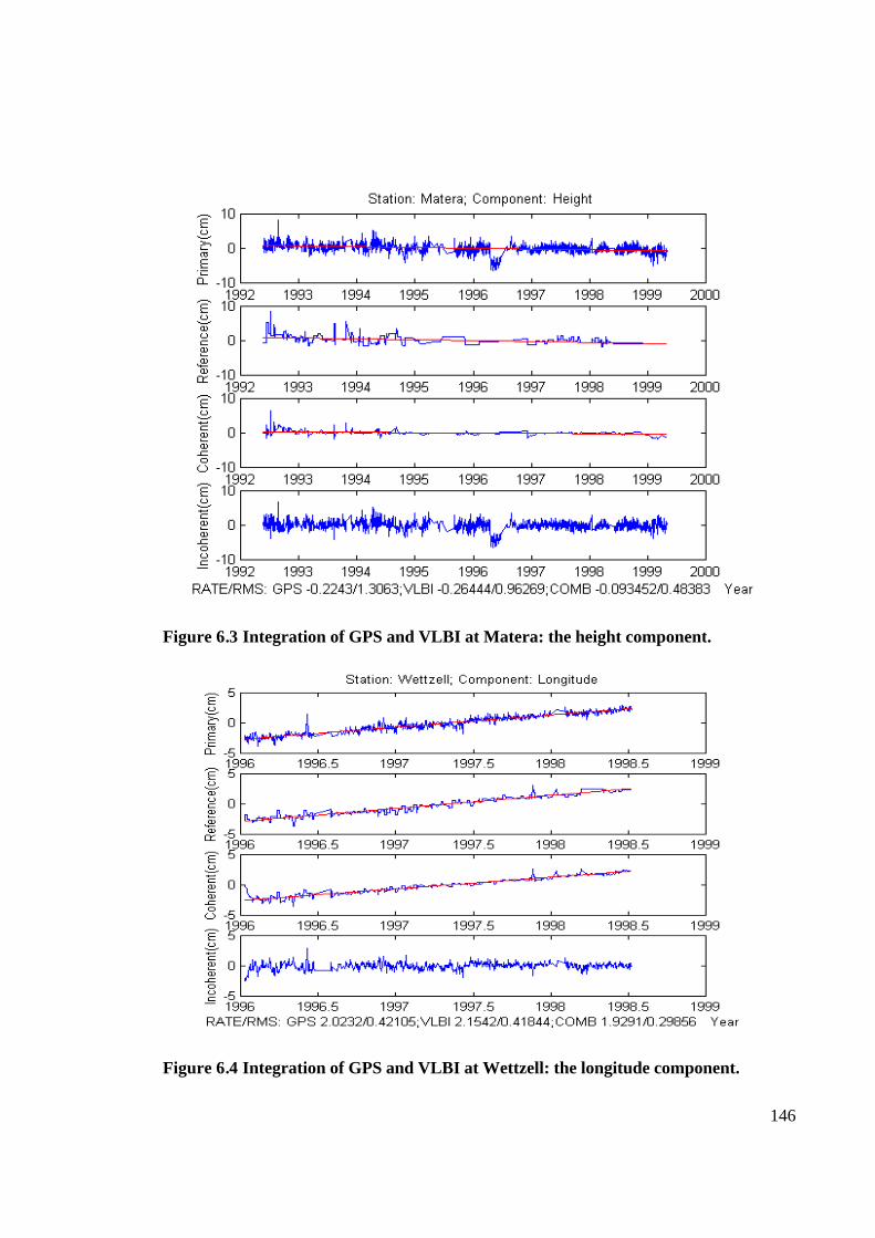
146

Figure 6.3 Integration of GPS and VLBI at Matera: the height component.

Figure 6.4 Integration of GPS and VLBI at Wettzell: the longitude component.

147

Figure 6.5 Integration of GPS and VLBI at Wettzell: the latitude component.

Figure 6.6 Integration of GPS and VLBI at Wettzell: the height component.

148

Table 6-3 Summary of GPS, VLBI, SLR and the integrated results (in cm).

Solutions

combined

GPS

VLBI JPL GPS1

GSFC VLBI2

rate 1.82 1.85 1.64 1.84 1.74 mLati-tude rms 0.58 0.45 0.69 0.42 0.34

rate 2.38 2.39 2.19 2.33 2.36 mLon-gitude rms 0.46 0.59 0.62 0.53 0.28

rate -0.09 -0.22 -0.26 -0.39 -0.12 mHeight rms 0.48 1.30 0.96 1.04 0.99

rate 1.14 1.30 1.30 1.32 1.35 wLati-tude rms 0.29 0.39 0.45 0.39 0.40

rate 1.92 2.02 2.15 2.05 2.04 wLon-gitude rms 0.29 0.42 0.41 0.43 0.40

rate -0.01 -0.01 0.33 -0.12 -0.10 wHeight rms 0.20 0.86 0.78 0.91 1.01

1: http://sideshow.jpl.nasa.gov/mbh/all/MATE.gif

http://sideshow.jpl.nasa.gov/mbh/all/WTZR.gif 2: http://lupus.gsfc.nasa.gov/vlbi.html

For the GPS-SLR combination, although generally the coordinates and velocities of each

SLR stations are estimated as global parameters and therefore the time series is not directly

available from such a process, it is possible to obtain a SLR time series if one evaluates the

coordinates of each station as local parameters (for single arcs).

Once the SLR time series is available, the common-mode signals derived from the three

combinations (GPS-VLBI, GPS-SLR, and GPS-VLBI-SLR) can be compared to see if they

are in agreement for both the Matera and Wettzell stations, which could facilitate the more

realistic determination of plate or fault movement. At Matera, also collocated is the space

geodetic technique PRARE, while at Wettzell available collocated techniques include

PRARE, GLONASS, gravimeter (super conducting), seismometer, meteorological sensors,

149

and water vapour radiometer. In future it is proposed to also integrate results from some of

these techniques.


Space geodetic techniques such as the GPS, VLBI, and SLR have been collocated at many

sites to address applications in the geosciences. A common-mode signal has been found

among the collocated results (coordinate time series) of GPS, VLBI and SLR, although

results from all these techniques are contaminated by different biases and errors. An

adaptive filter based on the Least-Mean-Square algorithm is proposed as the cross-

technique parallel temporal densification scheme to extract this common-mode signal by

inputting to the filter the GPS result as the primary sequence and VLBI and/or SLR results

as the reference sequences. Data from the Matera Station in Italy and the Wettzell Station in

Germany have been used to test the algorithm. The derived common-mode signal has better

repeatability than the individual results of GPS, VLBI and SLR. Further study is needed to

establish whether the movement rate determined by the derived common-mode signal is

more realistic than the individual results by comparing them with that from the NUVEL-1

Model.

In the following two chapters, spatial densification of CGPS measurements will be

discussed.

150

The approach suggested for so-called 'soft spatial densification' is the “double interpolation

and double prediction” (DIDP) technique for GPS and InSAR integration (Ge et al, 2000f;

Ge et al, 2000h). This Chapter begins with a brief introduction to the radar interferometry

(InSAR) technique. Then a detailed comparison between the two techniques - GPS and

InSAR shows that they are in fact very complementary to each other for crustal

deformation monitoring applications. For example, InSAR is very sensitive to a range of

errors such as atmospheric biases, satellite orbit errors, ground cover and temporal

decorrelation. While the latter two effects can only be reduced by careful selection of radar

band and SAR image pairs, the former two types of biases can only be significantly reduced

by incorporating GPS data. The DIDP technique is designed to take advantage of the

complementarity of GPS and InSAR.

7.1 Review of Radar Interferometry (InSAR)

There is a need in many fields of Earth science for accurate knowledge of topography and

topographic change at a variety of spatial scales and coverage areas. Radar interferometry

(or Interferometric synthetic aperture radar, InSAR for short) is a technique first suggested

in 1974 (Graham, 1974). After more than two decades of development, InSAR is now well

developed with many applications in mapping topography, topographic change

determination, and so on.

An image resulting from the phase difference between two SAR images acquired over the

same region is called an interferogram. The two SAR images may be acquired in the same

pass, as in the case of the Shuttle Radar Topography Mission (SRTM) and Airborne

Synthetic Aperture Radar (AIRSAR) (JPL, 1999). In this configuration the two antennas

are installed on the same platform, one of them sends out the radar signal while both

7 SOFT SPATIAL DENSIFICATION – THE INTEGRATION OF GPS WITH RADAR INTERFEROMETRY (INSAR)

151

receive the reflected signals from the surface of the Earth. This is referred to as 'single-pass

InSAR', and has the advantage that there is no problem of temporal decorrelation while the

disadvantage is that such a space-borne SAR system provides a big challenge in the orbit

maneuver and attitude control of the space vehicle, as was experienced during the SRTM

mission (SRTM, 2000).

If the two SAR images are acquired from two repeated SAR coverages of the same region,

the technique is referred to as 'repeat-pass InSAR'. It is much easier to build and deploy

such a SAR system. However, the temporal decorrelation is a big problem, which may limit

the SAR images that are suitable for InSAR processing. Nevertheless, for the purpose of

continuous crustal deformation monitoring, repeat-pass InSAR is the most suitable. Hence,

this Chapter will focus on the repeat-pass InSAR technique.

The SAR repeat-pass interferometry can generate digital elevation models (DEMs),

deformation maps, and temporal change maps (Zebker & Goldstein, 1986). Topographic

change measurement by InSAR was first demonstrated for Seasat L-band data (Gabriel et

al., 1989), and later with the spectacular contour map of co-seismic deformation associated

with the 1992 Landers earthquake in southern California obtained with the ERS-1 data

(Massonnet et al., 1993).

During the last decade SAR repeat-pass interferometry has been the subject of intensive

research. Although it is still not as operational a technique as GPS, it has been recognized

as a technique that yields important quantitative information such as height, large scale

deformation and (subtle) elevation change. It has the potential to routinely provide DEMs,

maps of deformation and change, and to allow a full geocoding of SAR imagery. A

growing number of applications have become feasible, and even more are being currently

investigated. Perhaps the most exciting new application of SAR interferometry is the 2-

dimensinoal mapping of crustal deformation with very high accuracy (mm- to cm-level).

Applications include earthquake deformation detection and monitoring, monitoring of

crustal movements, volcanic movement, landslides and land subsidence. Another

interesting area of research is the use of phase coherence for classification and change

152

detection. To exploit InSAR, two basic ingredients are required. The first is the acquisition

of two phase preserved SAR images of the same region but obtained at slightly different

viewing angles. These images may be obtained by the space-based SARs aboard ERS-1

(until June 2000), ERS-2, JERS-1 (until October 1998), and RADARSAT. Alternatively,

these images may be acquired by an airborne SAR sensor, either in single-pass or repeat-

pass modes. The second requirement is a set of image processing tools that combine the

two SAR images to create an interferogram and extract information from it.

InSAR is a process of using interference effects to determine lengths or changes in lengths

very accurately. This technique has some similarities to stereo-optical imaging in that two

images of the same area, viewed from different angles, are appropriately combined to

extract topographical information. However, a major difference between interferometry and

stereo imaging lies in the painstaking manual effort required in obtaining topographic

information from stereo-optical images. Meanwhile, inherent in SAR data, is distance

information that enables the automatic generation of topography models. This means that

DEMs can be generated using InSAR with greater automation than optical techniques.

Also, using the technique known as differential InSAR, surface deformations can be

measured with an accuracy and spatial measurement density which is unprecedented. Add

to this the ability of SAR to penetrate clouds and provide day and night operation, and it

becomes clear that InSAR has definite advantages over many conventional deformation

monitoring techniques.

SAR interferometry is possible because the technique measures both distance and radar

“brightness”. The distance information is encoded in phase, which is a fine scale

measurement of distance that is measured twice in two separate SAR passes. Distance

combined with incidence angle, and with the location of the SAR platform on each of the

two passes, gives a three-dimensional localization of points on the Earth’s surface. The two

SAR images, each containing brightness and phase information, can be used to produce one

interferometric data set from which height and other information is extracted.

153

In repeat-pass InSAR, interferograms are formed from repeated observations of the same

platform. With respect to the Earth, the satellite goes through a cycle of orbits, for example,

every 35 days in the case of ERS-2. This means that the satellite returns almost exactly to

the same position with respect to the Earth after 35, 70, 105, … days. On the first pass of

the satellite, a SAR image is acquired. After a period of time (one or more orbit repeat

cycles), the same area may be imaged again, thus acquiring the second SAR image.

The two SAR images are individually processed by a precision, phase preserving, SAR

processor to convert the “raw” radar signals into the black and white SAR images with the

phase information carefully preserved (e.g., the single look complex (SLC) image).

Sophisticated InSAR processing is then applied to register the two SAR images to an

accuracy of 1/8th of a pixel. Next, the phase differences in the two images are calculated by

subtracting the phase in one image from the phase in the other. The result is called an

interferogram. These phase differences in the interferogram wrap around in cycles of 360

degrees and must be unwrapped to obtain the absolute phase. The problem is very similar to

the carrier phase integer ambiguity resolution in GPS. It suffices to say that phase

unwrapping, although a complex process, is the key to high precision positioning. After

phase unwrapping, the absolute phase is converted to the various data products through

further processing.

In radar interferometry, two synthetic aperture radar images of a surface area are acquired

and combined into an interferogram, which contains the phase difference between the two

images. If the two images are acquired at the same time but at different sensor locations,

then the phase difference is related to the topography. If the scene is imaged from the same

location but at different times, then the phase difference is a record of topographic change.

If the scene is imaged from different locations and at different times, then the phase

difference is a record of both topography and topographic change. In a simplified geometry

where the radar antennas are looking directly orthogonal to their orbit motion, the

differential phase is given by (Zebker & Goldstein, 1986):

154

∆φ =4 4πλ

θ απλ

B rsin( )− + ∆ (7.1)

where θ is the look angle to a given image point,

B is the magnitude of the distance between the antenna locations, known as the

baseline vector,

α is the angle of the baseline vector measured from the orbital horizontal,

λ is the radar wavelength, and

∆r is the displacement of the image point along the radar line-of-sight from one

observation time to the next.

If the natural variation in ∆φ due to a reference surface at zero elevation is removed from

Eqn. (7.1), then

∆φ flat=4 4

00 0

πλ

θ αθ

πλ

Bz

rrcos( )

sin− + ∆ (7.2)

where θ 0 is the look angle not to the image point but to the reference surface,

r0 is the range to the reference surface, and

z is the height of the image point above the reference surface.

Eqn. (7.2) indicates that the first term is proportional to topography and the second term is proportional to the topographic change.

7.1.1 Environment of InSAR studies

Through the development of over two decades, more and more platforms are available to

provide images for InSAR studies. Though most remote sensing radars operate at

wavelength between 0.5cm to 50cm, L, C, and X are the most common radar bands used

for InSAR.

155

SAR data are available on C band (3.8-7.5cm) from the ERS-1, ERS-2 and RADARSAT

missions, on L band (15-30cm) from the JERS-1 and SEASAT missions, and on X band

(2.4-3.8cm) from the X-SAR mission. The characteristics of these platforms are

summarized in Table 7-1. Many organizations and companies in Australia, US, Japan,

Canada, France, Germany, Italy, China, etc., are providing SAR data.

The orbital parameters of ERS-1/ERS-2 could be adjusted to realize the three planned

repeat cycles of 3, 35 and 168 days. The transition from one orbital configuration to

another, to adjust the repeat cycle, requires up to two weeks to stabilize the orbits to within

1km of the nominal ground track. Therefore most of the time ERS-1/ERS-2 are running in

the 35 day repeat cycle.

SAR data are quite cheap compared to setting up a GPS reference station. Some SAR data

are actually provided free of charge for disaster-related InSAR studies (e.g., under the

“Open Sky” policy of NASA).

In order to obtain high quality InSAR images, the repeat cycle should be as short as

possible to provide a wide choice of SAR image pairs for processing. However, as

mentioned earlier, it takes some time for ERS-2 to stabilize after an orbit adjustment.

Furthermore, an exact repeat orbit is required for topographic change detection. Therefore

even a 3-day repeat cycle is not easy to achieve. With advances in space technology, twin-

satellite or shuttle SAR systems have been suggested to ensure a pair of correlated SAR

images are always available.

While the space shuttle is playing a more and more important role for InSAR studies, many

exciting new SAR missions are planned by different space agencies for the 21st century

(e.g. SAR 2000 by NASA). In short, the future InSAR application environment is very

favourable, and research on InSAR/CGPS integration is very topical.

156

Table 7-1 Most commonly used spaceborne platforms for InSAR.

Satellite SEASAT ERS-1/ERS-2 JERS-1 RADARSAT X-SAR Organization NASA/ JPL European

Space Agency NASDA of Japan

Canadian Space Agency

NASA/JPL

Time of launch

28 June, 1978

July 1991 / 1995

11 February, 1992

1995 9 April, 1994 (first flight)

SAR band L-band (23.5cm wavelength)

C-band (6cm wavelength)

L-band (24cm wavelength)

C-band X band (3cm )

polarization HH VV HH HH VV Orbit height 800km 785km 568km Repeat cycle 3, 35, or 168

days 44 days 24 days

SAR Antenna 10.74 x 2.16m

10.0 x 1.0m 4 x 12m

Resolution 25m 25m 18m 25m 10-200m Incidence angles

22 degrees 20-26 degrees 32-38 degrees

20-50 degrees

Number of Looks

4 4 3

Swath Width 100km 100km 75km 500km 15-90km Typical image area

80 x 80km 80 x 75km

Remarks first SAR satellite operated for 105 days until October 10, 1978

first commercial SAR satellite

first landing April 20, 1994; part of SIR-C/X-SAR

In the following sections some of the exciting applications of InSAR are briefly reviewed.

7.1.2 InSAR for DEM

Experience with the ERS-1, JERS-1, RADARSAT, and ERS-2 missions, even prior to the

SRTM mission, had established InSAR as a method for generating detailed and accurate

Digital Elevation Models (DEM) of the Earth's surface. Two missions, the ERS Tandem

157

Mission and the SRTM Mission, have contributed significantly to research on the use of

InSAR for DEM generation.

The ERS Tandem Mission started on the 16th August 1995 for a period of 9 months up to

end-May 1996, in which the two satellites ERS-1 and ERS-2 were both in 35-day repeat

orbits, but with ERS-2 following approximately 30 angular minutes behind ERS-1 in the

same orbital plane so that there was a 1-day interval between ERS-1 & ERS-2 observing

the same area of ground. The main driver for the Tandem Mission has been SAR

Interferometry and as a result a series of new and improved observations of geophysical

phenomena was made possible using the InSAR technique.

For the total period until May 1996, about 79% of all Tandem mission InSAR pairs are

suitable for DEM generation, 20% for potential use for Differential InSAR (ie land change

detection), and just 1% are unsuitable for InSAR. This high rate of suitable SAR images is

mainly due to the significant improvement in the phase coherence. The overall

improvement of interferogram quality (phase coherence) from the 1-day Tandem Mission

configuration, with respect to the 35-day and 3-day single satellite repeat cycles, has been

confirmed, although it is diffcult to quantify due to the strong dependence of coherence on

specific terrain conditions. Values of coherence as high as 0.7/0.8 have been observed for

some areas. However, there have been some snow-covered regions with extremely low

coherence (possibly due to summer melting).

Based on results achieved with ERS-1 and ERS-2, the improved coherence from the

Tandem Mission data is estimated to result in DEM rms height errors of less than 10m

across the complete 100 x 100km image, and less than 2m for local regions within the

image, under favourable conditions. This highly accurate and consistent DEM can play a

very important role in the DEM + InSAR approach for deformation monitoring.

The Shuttle Radar Topography Mission (SRTM) is illustrated in Fig. 7.1, in the form of a

computer-generated view of the Space Shuttle Endeavour flying above Earth's surface

during 11-22 February 2000. The SRTM Mission has collected three-dimensional

158

measurements of nearly 80% of the Earth's land surface, home to nearly 95% of the world's

population, except near the poles, with an accuracy of better than 16 metres.

With its radars sweeping most of the land surfaces of the Earth, SRTM acquired enough

data during its ten days of operation to obtain the most complete near-global, high-

resolution database of the Earth's topography. To acquire topographic (elevation) data, the

SRTM payload was outfitted with two radar antennas. One antenna was located in the

shuttle's payload bay, the other on the end of a 60m mast that extended from the payload

pay once the shuttle was in space. Additional C-band imaging antenna and improved

tracking and navigation devices were also incorporated.

All of the radar data was collected during the single, 11-day shuttle mission, and will be

processed to the same specification. Collecting and processing the data in this way ensures

that the SRTM-generated topographic maps will have the same quality. The resulting data

will provide 3-D images of the Earth's surface, which can be used to help study drainage

patterns and land surface changes over time. The data's military applications include

mission planning and rehearsal, modelling and simulation.

Figure 7.1 Computer-generated view of the Space Shuttle flying above Earth's surface

in the Shuttle Radar Topography Mission (SRTM) (JPL, 1999).

159

The ERS Tandem Mission and the SRTM Mission generated a unique and valuable data set

with important exploitation potential for years to come.

7.1.3 InSAR for deformation (elevation change)

Each year there are about 10 large earthquakes globally (among them about 3 occurring on

land which can be studied with InSAR). These events cause thousands of deaths and

considerable property damage. For example, the 1995 Kobe earthquake in Japan resulted in

over 5000 fatalities and damage estimates exceeding $100 billion. The geoscience

community therefore has a pressing need of a global data set of densely sampled pre-

seismic, co-seismic and post-seismic observations of crustal deformation. SAR

Interferometry has the potential to provide that data set, together with other techniques such

as GPS. As an extension of the basic InSAR technique, the Differential InSAR could allow

the detection of very small (mm to cm level) movements of the land surface, as

demonstrated with the ERS-1 repeat data for the 1992 Landers earthquake in California

(Massonnet et al., 1993).

As a matter of fact, due to its very high spatial coverage and cost effectiveness, many

earthquakes have been studied using InSAR:

• 28 June 1992 - Landers, California (Massonnet et al., 1993a; 1994; 1996);

• 17 January 1994 - Northridge, California (Murakami et al., 1996);

• 17 January 1995 - Kobe, Japan (Ozawa et al., 1997);

• 27 May 1995 - Sakhalin, Russia (Fielding et al., 1996,;Tobita et al., 1998);

• 13 May 1995 - Kozani-Grevena, Greece (Clarke et al., 1997);

• 17 May 1993 - Eureka Valley, California (Peltzer & Rosen, 1995);

• 1995 - Hyogoken-Nanbu, Japan (Murakami et al., 1995);

• 1993 - Izu Peninsula, Japan (Fujiwara et al., 1998a); and

• 26 March 1997 - Kagoshima-ken-hokuseibu, Japan (Fujiwara et al., 1998b).

160

This is far from a complete list. Some of the earthquakes were studied by several

researchers from different institutions, some were studied by the same researcher several

times, and some researchers have studied several quakes. More recently, InSAR has also

been applied to study the Mw 7.1 Hector Mine Earthquake in near-real time (Sandwell et

al., 2000). Colourful InSAR results on earthquakes have been used to derive fault models

that can be compared with those derived from seismic data; to estimate the co-seismic

deformation; to detect the fault-zone collapse; and so on. Seismologists have benefit greatly

from the InSAR results, as never before has the co-seismic deformation on seismic faults

been observed in such a comprehensive manner.

The following volcanoes have been studied with InSAR:

• Mount Etna, France (Briole et al., 1997);

• New Trident, Alaska (Lu et al., 1997);

• Merapi, Indonesia (Briole et al., 1997);

• Kilauea, Hawaii (Gaddis et al., 1989);

• Kunlun Mountains, western China (Guo et al. ,1997); and

• Mt. Vesuvius, Italy (Mouginis-Mark et al., 1993).

Volcanoes are ideal test sites for InSAR due to the absence of vegetation.

Other InSAR applications of elevation change determination include landslides (Fruneau et

al., 1996) and terrain subsidence (Rosen et al., 1997).

7.1.4 Other InSAR applications

Other main application domains of InSAR include: ice surface motion (for glaciology)

(e.g., Goldstein et al., 1993), and land surface change/classification (for forestry /

agriculture) (Wegmuller & Werner, 1995). For the study of glacial motion, maps of ice

motion velocity vectors have been derived from both ERS and JERS InSAR. It is thought

that the technique will work best during winter when the potential for daytime melting (and

161

consequent loss of coherence) is minimized. For land surface change / classification, results

with the ERS Tandem Mission confirm the potential for land surface cover discrimination

when coherence is combined with the radiometry.

However, the most exciting new application of InSAR is the two-dimensional mapping of

large scale surface deformation with very high sensitivity. These deformation maps can be

used to detect and monitor land deformation due to earthquakes, crustal movements,

landslides, volcanic activity (subsidence and absidence), underground mining activity and

water or fluid extraction (causing land subsidence).

7.2 Comparison Between CGPS and InSAR

Global continuous GPS (CGPS) stations, such as deployed for the International GPS

Service (IGS), provide the tracking data for determining precise satellite ephemerides and

for defining the terrestrial reference frame. The IGS therefore supports the wide application

of continuous GPS regional arrays for geodetic studies of crustal deformation. Many CGPS

networks have been set up in recent years, such as the Japanese GEONET, and the

Southern California Integrated GPS Network (SCIGN), by the Jet Propulsion Laboratory.

Many more countries are constructing their own CGPS networks, such as China, South

Korea, Taiwan, Hong Kong, Germany, U.K., Singapore, Russia, to name but a few. Data

from CGPS arrays are also used in meteorological research projects to test the feasibility of

operational mapping of the tropospheric water vapour, and ionospheric disturbances.

Most CGPS arrays are now sampling data at an interval of 30 seconds, although some can

sample at a one second interval. New GPS receivers can make as many as 10 to 20 samples

per second. Therefore CGPS receivers could provide temporally very dense GPS

observations. The high temporal resolution is the most significant characteristic of CGPS.

These CGPS arrays may be spatially dense enough for applications such as navigation,

RTK, etc. They are not dense enough, as a rule, for characterizing or monitoring seismic

faults. For this purpose sub-km level spatial resolution is required, which is hard to achieve

with CGPS networks. GEONET, the world's densest CGPS array, has receivers spaced at

162

an average 25km.

InSAR, on the other hand, exhibits around 25m spatial resolution (Table 7-1). Without the

need for any ground-based receiver or cooperative target, InSAR can virtually monitor

every corner of the Earth. But InSAR is very sensitive to errors such as atmospheric effects

(tropospheric delay, ionospheric delay, etc.), satellite orbit error, condition of ground

surface and temporal decorrelation. When present in the InSAR image, these errors can be

very misleading and lead to misinterpretation. However, there is no way to eliminate them

using only SAR data. Furthermore the repeat cycle of 35 to 44 days of SAR satellites can

not provide enough temporal resolution for applications such as monitoring terrain

subsidence due to underground mining, distinguishing deformations before, during, and

after earthquakes or volcano eruptions, and so on.

Table 7-2 provides a brief comparison of the two techniques. Since data from CGPS arrays

can be used to map tropospheric water vapour and ionospheric disturbances, these results

can be used to remove atmospheric effects in InSAR. With the support of SLR and VLBI,

GPS coordinates can be considered as being 'absolute' in the sense that they are tied to a

well-defined terrestrial reference system. While assuming that there are no displacements at

a few points (reference points) in a radar image in data processing, InSAR results are

relative measurements. GPS measurements on the reference points in a SAR image can also

be used as constraints to mitigate the influence of SAR satellite orbit errors. On the other

hand, InSAR results, with its high spatial resolution, can be used to densify GPS

observations in a spatial sense. Moreover, even when the GPS networks are densified, in

order to recover the signature of active faults the station configuration design may not be

ideal. Interpolation at these points, based on the GPS results from a well-designed station

network, can provide a good quality control measure.

Therefore it is obvious that the two techniques are complementary. The integration of

InSAR/GPS could measure deformation to 1 mm/yr precision with unprecedented spatial

coverage. Such a InSAR/GPS system would be able to determine displacement at millions

of points, rather than the few hundred being measured with current geodetic methods (e.g.

163

the 947 stations of the GEONET).

Table 7-2 Comparison of CGPS and InSAR.

CGPS InSAR Observable three component displacement

( horizontal and vertical, accurate in horizontal, inaccurate in vertical)

change of distance from ground to satellite (one component, may be divided to an accurate vertical and inaccurate horizontal)

Temporal resolution

almost continuous ( usually daily position solutions, can be one or even 30 samples per second)

periodical (every 35 days for ERS-1, 44 days for JERS-1, 1 day for ERS Tandem Mission)

Spatial coverage and resolution

discrete stations (highest resolution of about 25km in Japan)

continuous global coverage (25m x 25m resolution)

Satellite 24 GPS satellites one SAR satellite Receiver on ground

required (at least two to achieve high accuracy)

None

The integration of InSAR and GPS was first suggested in 1997 (Bock et al., 1997). The

Double Interpolation and Double Prediction (DIDP) approach for InSAR/GPS integration

was proposed in 1997 (Ge et al., 1997a&b). The algorithmic basis and some results of

DIDP are presented in this Chapter.

7.3 GPS and InSAR Integration – the "Double Interpolation and Double Prediction"

(DIDP) Approach

In the DIDP approach the first step is to derive atmospheric corrections to InSAR from

CGPS analyses. Analysis of the GPS data can give estimates of precipitable water vapour

(in a technique referred to these days as "GPS meteorology"), as well as the ionospheric

delay (possible because of the available dual-frequency GPS observations). The second step

164

is to remove or mitigate the SAR satellite orbit errors by using GPS results as constraints.

In a third step the CGPS observations, separated by one or several InSAR repeat cycles

within the SAR image, are 'densified' onto a grid. This is done by interpolation in the

spatial domain using as a basis a distribution model derived from the GPS-corrected InSAR

results. The densified gridded values are then interpolated in the time domain using as a

basis a dynamic model derived from the daily, hourly, or even 30 second sampling rate of

the CGPS data series, incorporating known geophysical information such as the locations

and geometries of active faults (Ge et al., 1999b). The adaptive filter can be used in this

step. In a fourth step, based on the double interpolation result, forward filtering (e.g.

Kalman filtering) can be used to predict the crustal deformation at all points on the grid - in

effect a double prediction in both the temporal and spatial domains.

7.3.1 Deriving atmospheric correction to InSAR from CGPS

In the DIDP approach the first step is to derive atmospheric corrections to InSAR using

CGPS data (Bevis et al, 1992). It is well known that the accuracy of InSAR measurement is

limited mostly by atmospheric propagation heterogeneity (due to the highly variable

distribution of atmospheric water vapour) in space and time (e.g. Massonnet et al, 1995).

Atmospheric refraction artefacts in the InSAR result may introduce errors as large as three

fringes locally, in the case of exceptional conditions. Therefore they have to be corrected

before InSAR results can be used for deformation analysis.

On the other hand, although the primary purpose of almost all CGPS arrays is to address

geodetic applications, they may also produce estimates of the tropospheric zenith delay in

the immediate vicinity of the GPS station as a byproduct of data processing. Using CGPS

data it is possible to map the tropospheric zenith delay with high resolution in both space

and time. This, in turn, can be used as an atmospheric 'correction' to the InSAR result. Such

atmospheric 'corrections' generated from CGPS data will soon be generally available

through the IGS and other services, as there is a growing interest in the monitoring of

atmospheric water vapour.

165

Water vapour is one of the most significant constituents of the atmosphere since it is the

means by which moisture and latent heat are transported, and hence cause "weather". Water

vapour is also a greenhouse gas that plays a critical role in the global climate system.

Despite its importance to atmospheric processes over a wide range of spatial and temporal

scales, water vapour is one of the least understood and poorly described components of the

Earth's atmosphere.

While an important goal in modern weather prediction is the improvement of short-term

cloud and precipitation forecasts, the ability to do so is severely limited by the lack of

timely and accurate water vapour information. Traditional water vapour observing systems

include radiosondes, surface-based radiometers, satellite-based radiometers, and some

research aircraft. Each of these systems has advantages and limitations. Although it also has

limitations, many researchers believe that ground-based CGPS will be most useful as an

element of a composite upper-air observing system. In this role it will provide frequent

water vapour measurements to constrain numerical weather prediction models, as well as

independent calibration and validation of satellite measurements.

The principle of using GPS data to measure water vapour is based on the fact that GPS

radio signals are slowed as they propagate from the GPS satellites to ground-based

receivers, passing through layers of the Earth's atmosphere: the ionosphere and the neutral

atmosphere. This slowing delays the arrival time of the transmitted signal from that

expected if there were no intervening media. It is possible to correct for the ionospheric

delay, which is frequency dependent, by using dual-frequency GPS measurements. The

delays due to the neutral atmosphere, however, are effectively non-dispersive at GPS

frequencies and so cannot be corrected in this way. They depend on the constituents of the

atmosphere, which are a mixture of dry gases and water vapour.

In a ground-based GPS system, the signal delays from several (at least four, but typically

six or more) satellites in view are simultaneously measured. These delays are

mathematically adjusted (scaled) such that all satellite signals are treated as having been

transmitted from directly overhead (at the zenith) simultaneously, using the mapping

166

function:

MT(θ) = 1/sin θ (7.3)

where θ is the elevation angle from receiver to the satellite. The averaged vertically-scaled

signal delay introduced by the atmospheric constituents is called the Zenith Total (or

Tropospheric) Delay (ZTD). ZTD can be separated into two components, the zenith

hydrostatic delay (ZHD) and the zenith wet delay (ZWD):

)()( 00 θθ wwhh MLMLL ∆+∆=∆ (7.4)

where )(__)( θθ wh MandM are the hydrostatic and wet mapping functions respectively.

00 __ wh LandL ∆∆ are ZHD and ZWD respectively (in mm).

The ZHD is calculated by measuring the surface pressure and applying a mapping function.

The ZWD can be viewed as a stochastic process, and the process parameters can be

estimated using a Kalman filter. In fact, both stochastic and deterministic algorithms for

atmospheric modeling are employed in high precision GPS software such as GIPSY,

GAMIT and the Bernese package.

Suppose the ZTD at GPS station i at the SAR image acquisition time t is )(tLi∆ using Eqn.

(7.4), the atmospheric correction derived from GPS data to the InSAR result on the image

point of station i will be:

)()( 12 tLtLL iii ∆−∆=δ (7.5)

where t1 and t2 correspond to the imaging time of the two SAR images used in the

interferometric processing. The atmospheric correction for other image points can be

interpolated from the GPS stations.

167

7.3.2 Remove or mitigate SAR satellite orbit errors by using GPS results as

constraints

The second step of DIDP is to remove or mitigate SAR satellite orbit errors by using GPS

results as constraints. For this purpose, metal corner reflectors can be co-located with, or

'tied' precisely to, some GPS sites on the ground. The SAR data covering each of these GPS

sites thus correspond to a precisely-located point, and hence could be used to provide 3-D

corrections to the spacecraft orbit, and hence improve the accuracy of the ground

displacement measurement.

Fig. 7.2 illustrates the InSAR geometry. The radar beam is transmitted to the ground from

antenna A1. After scattering at the ground point G, the radar wave is received by antennas

at both A1 and A2. The distance between A1 and A2 (the baseline length) is B (exactly 60m

in the case of the Shuttle Radar Topography Mission, the length of the mast (JPL, 1999))

and the radar look angle is θ. The GPS heights of the antenna A1 and the ground point G

are H and h respectively. H can be estimated from the SAR satellite ephemeris, but usually

not precisely enough for deriving DEM or deformation information (because it is one of the

orbit errors to be mitigated), although for SRTM data it is precisely known because GPS

receivers were flown aboard the space shuttle. The h is usually an unknown to be solved by

InSAR but is known precisely if a GPS receiver and corner reflector are employed at the

control point. Suppose β = ∠G A1 A2 can be calculated from the orientation of the baseline,

then the geometric distance r between A1 and G can be calculated as:

βδδcos22

22

B

Br

+−

= (7.6)

where δ can be calculated from the phase difference ϕ from InSAR as:

168

λπ

ϕδ

2= (7.7)

where λ is the radar wavelength. Therefore, the SAR vehicle height estimated from the

ground control point information is:

θcosrhH += (7.8)

Several estimations of H can be obtained if there are several ground control points. By

giving different weights to both these estimates and the H derived from the SAR satellite

ephemeris in a least-squares process (Giordano & Hsu, 1985), the orbit errors can be

effectively reduced.

A1 A2

H

B

rr + δδ

θ

G

h

Figure 7.2 The radar interferometry geometry (after Mouginis-Mark, 2000).

169

7.3.3 Densify observations by double interpolation

The atmospheric and orbit corrections dealt with in the previous two sections yield GPS-

corrected InSAR results. In the third step of DIDP, the CGPS observations separated by

one or several InSAR repeat cycles are densified in a grid manner by interpolation in the

spatial domain based on the GPS-corrected InSAR results (geophysical information has

been incorporated in the distribution model for this interpolation) (Ge et al., 1999). Then

the densified grid observations are interpolated in the time domain based on the daily,

hourly, or even 30 second sampling rate CGPS time series (adaptive filtering based on the

least-mean-square algorithm has been used to extract the dynamic model for this

interpolation) (Ge, 1999).

7.3.3.1 Distribution Model For Interpolation Based on InSAR Result and Incorporating

Geophysical Information

To start the interpolation process, an irregular grid pattern is formed based on the locations

of the stations in the GPS network.

As indicated in Fig. 7.3, the latitudes and longitudes of the GPS stations are read from a

(sequential) data file. Here Nij (i, j=1, 2, 3, and 4) refers to the latitude for the ith station in

the file and it ranks j among the latitudes for all the GPS stations. Eij stands for longitude

and is analogous with Nij. Then the latitudes Nij and longitudes Eij are sorted according to

their values (i.e. index j). The sorted latitudes and longitudes are then combined to form the

grid (Nij, Eij), consisting of both existing GPS stations (denoted by “G”) and points to be

interpolated (denoted by “I”). The important feature of the two dimensional sorting is that

the attributes of GPS stations (index i) are maintained so that no interpolation operation is

needed on grid points of GPS stations. Therefore, the algorithm carries out an “indexed

sorting”.

170

It can be seen from Fig. 7.3 that there is one and only one GPS station in both the rows and

the columns on the transformed grid. In practical applications, however, there may be two

or more when the CGPS array is very dense and some of the stations are very close, or in

the contrary situation, there may be none in a row or column when the CGPS array is very

sparse but a relatively dense 'densification' is desired.

Coordinates of GPS stations (e.g.,4)

Latitude Longitude

N12 E13

N23 E21

N31 E34

N44 E42

Transformed grid

E21 E42 E13 E34N31 I I I GN12 I I G IN23 G I I IN44 I G I I

Figure 7.3 An irregular grid formed by indexed sorting.

In order to interpolate objectively, it is proposed that geophysical information be

incorporated. It is well known that the movements of GPS stations on the two sides of a

fault can be significantly different, therefore it is important to classify the stations and the

intended interpolating points according to their positions in relation to the fault. The open-

(Fig. 7.4) and closed- (Fig. 7.5) curve models have been designed to describe the geometric

characteristics of faults. In the open-curve model the region of interest is divided into upper

(or left) and lower (or right) sub-regions by an open curve. This model should be adequate

for most seismic faults.

An algorithm has been developed to automatically identify to which sub-region a station or

an interpolating point belongs. Assume the unit vectors of latitude is →

i and longitude is →

j ,

from an arbitrary point on the fault (Ni, Ei) to the GPS station (GS) at (NG, EG) the vector

can be expressed as:

→→→

•−+•−= jEEiNNG iGiG )()( (7.9)

A minimum search of vector length is performed to find min|| ),( =→

ii ENG

171

Therefore, a GS local fault vector can be written as:

→

+

→

+

→

•−+•−= jEEiNNF iiiiG )()( 11 (7.10)

From an arbitrary point on the fault (Nj, Ej) to the interpolating point (IP) at (NI, EI) the

vector can be expressed as:

→→→

•−+•−= jEEiNNI jIjI )()( (7.11)


jj ENI

Then, an IP local fault vector can be written as:

→

+

→

+

→

•−+•−= jEEiNNF jjjjI )()( 11 (7.12)

From Eqs. (7.9) to (7.12) a “decision” can be made: if )()(→→→→

×•× IFGF IG > 0 the GPS

station and the interpolating point are on the same side of the fault. Otherwise they are on

different sides of the fault.

Figure 7.4 Open-curve model: one GPS station and one interpolating point case.

In the closed-curve model the region to be studied is divided into 'outside' and 'inside' sub-

regions by a closed curve. This model is appropriate for applications such as volcano

deformation monitoring.

172

Figure 7.5 Closed-curve model: one GPS station and one interpolating point case.

A different algorithm for this model is developed to automatically identify in which sub-

region a station or interpolating point belongs to. Again assume the unit vectors of latitude

is →

i and longitude is →

j . From the GPS station (GS) at (NG, EG) to an arbitrary point on

the fault (Ni, Ei) the vector can be expressed as:

→→→

•−+•−= jEEiNNG GiGi )()( (7.13)


ii ENG

The GS primary vector is thus determined as:

→→

= GL1 (7.14)

Then a minimum distance search from an arbitrary point on the fault to the GS primary

vector can determine ),( jj EN , which is used to calculate the GS secondary vector:

→→→

•−+•−= jEEiNNL GjGj )()(2 (7.15)

173

From Eqns. (7.14) and (7.15), a “decision” can be made: if 21

→→

• LL > 0 the GPS station is

outside of the fault. Otherwise it is inside the fault. The position of the interpolating point

relative to the fault can be determined in the same way.

The combination of open- and closed-curve models can deal with comparatively complex

fault systems. After the classification of GPS stations and the intended interpolating points

into different groups, a distribution model for interpolation for each group based on the

GPS-corrected InSAR results is proposed, as illustrated in Table 7-3. After developments

over more than two decades, InSAR is now capable of addressing many applications such

as mapping topography, detecting topographic change, etc. InSAR has approximately 25m

spatial resolution. Without the need for any ground-based receiver or cooperative target, it

can virtually monitor every corner of the Earth. But InSAR is very sensitive to errors such

as atmospheric effects (tropospheric delay, ionospheric delay), satellite orbit error,

conditions of the ground surface and temporal decorrelation. When presented in the InSAR

image, these errors can result in misleading interpretation. There is at present no way to

eliminate them using SAR data alone. Therefore, a distribution model for interpolation

based on both GPS and InSAR results is proposed, as given in Table 7-3. In some sites of

interest (Sites 1 to 4) there are both GPS and InSAR results for the deformation (the CGPS

results may have to span one or more InSAR repeat cycles depending on the availability of

suitable SAR image pairs). But in most other sites (Sites 5, 6, …) there will only be InSAR-

derived results. All of the results are input into a least-squares adjustment (e.g. Giordano &

Hsu, 1985). The adjusted results, which form the distribution model for interpolation in

spatial domain, are used as constraints later on to scale the time series generated at the

interpolated points based on the dynamic model.

174

Table 7-3 Distribution model based on InSAR information.

Interested site

GPS result

InSAR result

Least-square adjusted result

1 G1 S1 A1 2 G2 S2 A2 3 G3 S3 A3 4 G4 S4 A4 5 S5 A5 6 S6 A6

It is important to have overlapping GPS and InSAR results over the active fault region so

that the GPS results can be used to calibrate out some errors in the InSAR results. But this

condition is very hard to satisfy (Bock & Williams, 1997). It is hoped that the densification

of CGPS and new missions for InSAR such as the Shuttle Radar Topography Mission

(SRTM), Airborne Synthetic Aperture Radar (AIRSAR), Geographic Synthetic Aperture

Radar mission (GeoSAR), and Lightweight Synthetic Aperture Radar (LightSAR) (JPL,

1999), will ease such difficulties.

Fig. 7.6 is an example of the deformation distribution model based on both InSAR and GPS

for the 1992 Landers Earthquake, obtained following such an approach. The geocoded

InSAR result and GPS result for 38 sites for the 1992 Landers Earthquake epicenter region

were kindly provided by courtesy of Dr Massonnet of CNES, France (Massonnet et al.,

1993) and Dr Freymueller of the University of Alaska (Freymueller et al, 1994)

respectively. In order to derive the distribution model for interpolation in the spatial

domain, GPS sites were first matched with their imaging points in the InSAR result. Then

the GPS displacements were projected to the change in range in the direction which points

towards the satellite. Meanwhile, the InSAR result was resampled. Having obtained both

InSAR and GPS results, they were least-square adjusted as outlined above. Fig. 7.6 is a plot

of the adjusted result (Ge et al, 1999b), which is not significantly different from the InSAR

alone result (Massonnet et al., 1993) due to the fact that some GPS stations have been used

as ground control points in the InSAR data processing, and that the InSAR and GPS results

employed are generally in good agreement. However, this will by no means lessen the

importance of InSAR/GPS integration for deriving the distribution model.

175

Figure 7.6 A deformation distribution model based on both InSAR and GPS for the

1992 Landers Earthquake.

7.3.3.2 Dynamic Model For Interpolation Based on CGPS Times Series

After the classification of GPS stations and the intended interpolating points into different

groups, CGPS results sampled daily, hourly, or even every 30 second from stations in the

same sub-region are used to derive a dynamic model, which is then used to interpolate in

the time domain at grid points in the same sub-region. Figs. 7.7 to 7.9 shows an example of

a dynamic model extracted using an adaptive filter based on the least-mean-square

algorithm (Ge, 1999) for daily CGPS results from two closely located stations in the same

classified group: stations BRAN and LEEP of the Southern California Integrated GPS

176

Network (SCIGN).

In each figure, the first two plots are latitude time series for stations BRAN and LEEP

respectively. The third plot is the model derived using an adaptive filter, which can be used

as a dynamic model for interpolation in temporal domain. The characteristic change in the

model near day 300 indicates that the filter does need some time before it can identify the

coherent features between the two inputs. The last plot is the local monument movement at

BRAN output by the filter. It is well known that the local monument movement for a

continuous GPS station can lead to very misleading results. Although much effort has been

made to improve the design of the monument, this local movement remains a significant

concern in any interpretation. If the GPS time series from individual CGPS stations, as

shown in the first two plots of Figs. 7.7 to 7.9, are used directly as dynamic model for

interpolation, all the deformations at grid points around the stations will be biased.

Therefore it is important to separate the local monument movement from the crustal

deformation due to plate or fault motion. Fortunately, since the local monument movements

are independent, while the crustal deformations at stations in the same sub-region are

strongly correlated (as evident in Figs. 7.7 to 7.9), the adaptive filtering can be employed to

decompose them. Even though the two time series from BRAN and LEEP are very

different, the derived model in the third plot can function reliably as the dynamic model.

If there is only one CGPS station in the sub-region, its time series is used directly as the

dynamic model. If there are more than two CGPS stations in the same sub-region, one of

them is used as the primary station and the others are used to provide reference sequences,

and the adaptive filter is extended to handle a single primary input and multiple reference

inputs system, rather than the single reference input system as shown in Figs. 7.7 to 7.9.

After the double interpolation in this step, deformations at the GPS sites and interpolated

points are both spatially and temporally dense enough to be used to prepare an 'animation'

of how the crust deforms.

177

Figure 7.7 Dynamic model extracted using adaptive filtering on CGPS results from

BRAN and LEEP stations of SCIGN (latitude component, data courtesy of Jet

Propulsion Laboratory, NASA, USA).

178

Figure 7.8 Dynamic model for the longitude component.

Figure 7.9 Dynamic model for the height component.

179

7.3.4 Extrapolate quasi-observations by double prediction

In the fourth step of DIDP, based on the double interpolation result (quasi-observations) of

the third step, forward filtering (Kalman filtering) is used to predict the crustal deformation

at all points on the grid. This is in fact a double prediction in both the time and spatial

domains, which could facilitate the use of the DIDP technique for applications such as the

prediction of volcano eruption or earthquake ruptures. Moreover, this step is very important

in the three-step reliability test (RT) for DIDP. In the first step of RT, the CGPS and SAR

data are processed to yield a CGPS time series and the InSAR image respectively. In the

second step of RT, the CGPS time series from some of the sites are used together with the

InSAR image in the double interpolation to predict CGPS time series for the rest of the

CGPS sites. The CGPS time series for these latter sites, from both observation and

prediction, are compared to test the reliability of the double interpolation. In the third step

of RT, the CGPS time series from all the sites in one SAR repeat cycle are used, together

with the InSAR image for the same SAR repeat cycle in the double interpolation, to

generate quasi-CGPS time series for all the points on a grid. These quasi-CGPS time series

are then used in the double prediction to yield the deformation in the next SAR repeat

cycle. The predicted deformation is compared with the CGPS and InSAR results in the next

repeat cycle to further test the reliability of the double prediction.


The Double Interpolation and Double Prediction (DIDP) approach for integrating InSAR

and GPS results in the soft spatial densification scheme has been described in this Chapter.

In the DIDP approach, the first step is to derive the atmospheric corrections to InSAR from

the CGPS measurements.

The second step is to remove or mitigate the SAR satellite orbit errors by using GPS results

as constraints. Metal corner reflectors are co-located with (or tied precisely to) some GPS

sites. The SAR data covering each of these GPS sites thus correspond to a precisely-located

point, and hence could be used to provide 3-D corrections to the spacecraft orbit, thus

180

improving the accuracy of the ground displacement measurement. These atmospheric and

orbit corrections yield GPS-corrected InSAR results.

In the third step, the CGPS observations separated by one or several SAR repeat cycles are

densified in a grid by interpolation in the spatial domain, based on the GPS-corrected

InSAR results but according to a distribution model. Then the densified grid observations

are interpolated in the time domain, based on a dynamic model derived from the daily,

hourly, or even 30 second sampling rate of the CGPS time series.

Geophysical and InSAR information have been incorporated in the interpolation of GPS

measurements. The indexed sorting algorithm is very effective in forming an irregular grid

pattern for interpolation and maintaining the “attributes” of the GPS stations. The

combination of open- and closed-curve models of a fault is suitable for dealing with

comparatively complex fault systems. CGPS data from the SCIGN have been used to

demonstrate that adaptive filtering can be successfully used to extract a dynamic model

from the GPS time series of stations in the same classified group. A deformation

distribution model for interpolation in spatial domain was derived based on both InSAR

and GPS results for the 1992 Landers Earthquake.

In the fourth step, based on the double interpolation result of the third step, forward

filtering (using a Kalman filter) is used to predict the crustal deformation at all points on the

grid, which is in fact a double prediction in both the time and spatial domains.

Since a single SAR image usually covers an area of only 50km by 50km, the reliability of

spatial interpolation is guaranteed. Because GPS receivers are operating continuously, and

can achieve high accuracy, the DIDP method is, refer to Fig. 1.7, a promising strategy for

soft spatial densification to significantly improve the spatial, temporal and magnitude

resolution of ground deformation monitoring to 25m, 30 second and mm level respectively.

181

Hard spatial densification can be achieved either by deploying a sub-network of single-

frequency GPS receivers to in-fill the present CGPS arrays, typically involving the

integration of single- and dual-frequency GPS receivers in a so-called ‘inward hard spatial

densification’, or by deploying receivers at some geophysically strategic sites outside the

existing CGPS array so that combinations of different baselines can be used to, for

example, separate plate tectonic and seismic fault movements, in a so-called ‘outward hard

spatial densification’.

The 'inward hard spatial densification' is a cost-effective way of deploying many extra

receivers in local areas where the deformation patterns are likely to be very complex, such

as the junction of several active seismic faults, or where the receivers are more vulnerable

to damage (hence some backups are necessary), such as at active volcanoes. In this

densification scheme, the dual-frequency measurements are used to generate "error-

correction terms", which are used in a linear combination observation model for the

processing of the single-frequency measurements. In this way any GPS satellite orbit bias

and ionospheric delay can be largely eliminated, and the tropospheric delay, multipath and

observation noise can be significantly reduced. In this way it is possible to ensure sub-

centimetre relative accuracy (Rizos et al., 1999). Such a scheme is essentially the same as

that of the Virtual Reference Station (VRS) concept introduced in Chapter 3, although

different algorithms may be used to generate the "error-correction terms".

To test the effectiveness of such an 'inward hard densification' scheme, in August 1999

researchers from The University of New South Wales (UNSW) and from Japan's

Geographical Survey Institute (GSI) tested a hardware/software system design for a

continuously-operated ground deformation monitoring system based on low-cost GPS

receiver technology (Rizos et al, 1999). This UNSW-GSI experiment was undertaken using

8 HARD SPATIAL DENSIFICATION – INTEGRATING SINGLE- AND DUAL-FREQUENCY GPS RECEIVERS

182

data from the GEONET.

In order to densify such CGPS networks (important when high spatial resolution for the

monitoring of the deformation phenomenon is required), and to promote the use of the

CGPS technique in lesser developed countries, a significantly cheaper system architecture

is needed. The proposed design is an integrated, dual-mode network consisting of low-cost,

single-frequency GPS receivers across the area of interest, surrounded by a sparser network

of dual-frequency GPS receivers. Initial tests using the dual-frequency data collected at

selected stations in the GEONET network to simulate single-frequency data have already

shown that through enhanced data processing algorithms a CGPS network containing both

single-frequency and dual-frequency receivers would be able to deliver better than

centimetre level relative positioning accuracy (Rizos et al., 1998).

Chapter 8.3 will report the results of the first field tests carried out in the Tsukuba area of

Japan. The test network consisted of: (a) several stations of the GEONET network,

surrounding (b) an inner network of four single-frequency Canadian Marconi GPS

receivers installed by UNSW researchers (single- and dual-frequency GPS receivers are

compared in Chapter 8.1). The data from both the GEONET and the UNSW receivers were

processed using a modified version of the Bernese GPS Software Package. The software

first processes the GEONET GPS station data in order to generate empirical "corrections",

which are then applied to the double-differenced data of the GPS baselines located within

the test area enclosed by the dual-frequency CGPS stations (the algorithm and procedures

are briefly discussed in Chapter 8.2). These corrections have the effect of improving

baseline solution accuracy by up to an order of magnitude, even for baselines ranging up to

100km in length. The baselines connecting the inner network to the surrounding GEONET

stations are processed in a number of modes, including 24hr files (as is the standard

practice for geodynamic applications), and hourly data files (as in volcano deformation

monitoring applications). Chapter 8.5 draws conclusions on the basis of the results of the

UNSW-GSI experiment.

183

The 'outward hard spatial densification' is described in Chapter 8.4. To test this

densification scheme, CGPS observations from four stations distributed on both sides of the

Longitudinal Valley Fault in Taiwan and one station in Tsukuba (Japan) are processed to

generate baseline solutions, which are then used to separate plate tectonic and seismic fault

movements.

8.1 Comparison Between Single- And Dual-Frequency GPS Receivers

GPS-based volcano monitoring at Miyake-jima Island in Japan (Fig. 8.1) an example that

illustrates why the spatial densification is necessary. Four GEONET stations have been

installed on the Island: Stations 93059 (latitude 34 07 03 and longitude 139 30 25) and

93060 (latitude 34 03 20 and longitude 139 33 01) were installed in 1993, while Stations

960599 (latitude 34 05 25 and longitude 139 33 53) and 960600 (latitude 34 04 20 and

longitude 139 28 55) were installed in 1996. On 27 June 2000 the GPS Observation Group

was formed at the Earthquake Research Institute (ERI) of Tokyo University in response to

the increased volcanic activity associated with an earthquake swarm on 26 June 2000.

Since 15 July 2000 the three ERI CGPS stations and the 13 temporary CGPS stations have

become operational, and 32 temporary rapid static points have been surveyed on a regular

basis. Although 3 out of the 4 GSI CGPS stations were damaged during the volcanic

activity, crustal movements associated with the magma intrusion beneath the summit of Mt.

Oyama on the Island on June 26 and 27, the August 18 10:52 M6.0 earthquake, and the

August 18 17:00 eruption have been successfully monitored by this dense GPS network.

In summary, as is apparent from the figure, in an area smaller than 10km by 10km, there

are four GSI GEONET CGPS stations, three ERI CGPS stations, 13 temporary CGPS

stations, and 32 temporary GPS-surveyed points, all of which have played an important role

in mitigating the effects of the disaster. Without the newly installed ERI CGPS stations, the

temporary stations and the surveyed points, prediction of the volcanic eruption would not

have been so successful. Spatial densification of a GPS network such as this, therefore, can

provide not only necessary input to geophysical modelling but also some redundancy. Note

also that this is not an experiment run by a GPS manufacturer to promote the sale of

184

receivers, rather it is real and very recent field work carried out by ERI, which has

extensive expertise in the modelling of earthquakes and volcanoes.

Figure 8.1 GPS network for volcano monitoring at Miyake-jima, Japan (after ERI,

2000).

While it is important for the CGPS network to have a high enough spatial resolution in

order to monitor the deformation phenomenon associated with earthquakes and volcanoes,

Japan may be one of the few countries (if not the only one) which are capable of densifying

an existing CGPS network in such a short time, and with such a density. Moreover, even in

this example many rapid-static-surveyed points had to be established, which posed potential

185

threats to the lives of the GPS surveyors. Therefore, the proposed 'inward hard spatial

densification' scheme based on integrating single- and dual-frequency receivers is a

worthwhile topic of study.

Single-frequency receivers are widely used in navigation (in space and in the air, on land,

or at sea). Single-frequency observations are also adequate for short baselines using

conventional GPS surveying techniques.

However, dual-frequency receivers do offer significant advantages. They can be used to

eliminate the effects of ionospheric delay (which is a problem for baselines greater than

about 20-30km in length), they increase the reliability of the results over long baselines,

and they certainly increase the scope of GPS procedures available to the receiver operators.

Dual-frequency instrumentation is also essential for high productivity "rapid-static", "stop-

&-go" and "kinematic" GPS surveying procedures because of the advantages of dual-

frequency phase and pseudo-range data for rapid ambiguity resolution.

There is intensive R&D to improve the tracking performance on the L2 carrier wave. In

order to recover both carrier and code on the L2 signal when Anti-Spoofing is on, receivers

have to be built using techniques such as squaring, cross-correlation, code-correlation-plus-

squaring, and Z-tracking (Rizos, 1996). As a result, dual-frequency instruments usually are

hybrid, with code-correlating on L1, and proprietary codeless technology on L2.

Dual-frequency instruments are used mainly on geodetic and geodynamic applications,

which comprises a much smaller market than in the case of navigation applications.

Moreover, as mentioned above, they are much more complex and therefore are more

expensive than single-frequency receivers.

Is there an approach which can take the advantages of both single- and dual-frequency

receivers and yet still deliver high accuracy? The next section describes the proposed

scheme.

186

8.2 Inward Hard Spatial Densification – Integrating Single- And Dual-Frequency GPS

Receivers

Permanently operating GPS networks have been used for many years in support of geodetic

applications. Data from these networks are usually collected on a daily basis, centrally

archived at data centres, and are available via the Internet to users. Many of these users,

through the application of special carrier phase processing techniques, are able to achieve

relative station coordinate accuracies as high as a "few parts per billion" (sub-centimetre

accuracy for receiver separations up to a thousand kilometres or more). However, typically

"sub-parts-per-million" accuracies (sub-ppm: 0.1ppm implies an accuracy of 1cm in 100km

baseline) are considered to be indicative of "GPS Geodesy" techniques. The range of

applications that can be addressed using GPS Geodesy techniques is growing rapidly.

Though the CGPS spatial resolution, such as that of the GEONET, is now as high as about

25km, due to the high cost of dual-frequency GPS receivers they may not be established in

a dense enough configuration to address all of the geodetic applications. One of them, the

monitoring of pre-seismic or post-seismic faulting, requires sub-km resolution, as indicated

by the faulting length in Table 1-1.

One option for increasing the geodetic network's spatial resolution is to use low-cost GPS

receivers to densify the dual-frequency network, that is, the 'inward hard spatial

densification' scheme. The dual- and single-frequency stations are treated as reference and

user stations respectively. Another option is to integrate CGPS with techniques such as

differential Synthetic Aperture Radar Interferometry (InSAR) (i.e. the 'soft spatial

densification' scheme discussed in Chapter 7). As described in several previous studies (e.g.

Han, 1997; Rizos et al., 1998; Chen et al., 1999), hard densification data processing

strategies have been developed by the UNSW Group that can deliver sub-ppm relative

accuracy even for baselines up to 100km in length. Here the data processing algorithm is

briefly outlined.

The double-differenced observable can be written as:

187

∇∆φ = ∇∆ρ + ∇∆dρ + λ ⋅∇∆N − ∇∆dion + ∇∆d

trop + ∇∆dmp

ϕ + ε∇∆φ (8.1)

where ∆∇ represents the double-differencing operator; φ : the carrier phase observation in

units of metres: ρ : ( )= −x xS , xS is the satellite position vector, x is the station position

vector; d ρ : the effect of ephemeris errors (including SA effects, if any); λ : the wavelength

of the carrier; N: the integer ambiguity for a particular satellite-receiver pair; iond , tropd ,

φmpd and ε∇∆φ are the ionospheric delay, tropospheric delay, multipath effect and the carrier

phase observation noise for a particular one-way observation, respectively (Han, 1997).

From Ibid (1997), Eq (8.1), through a linear combination (assume the number of GPS

reference stations is three), can be written as:

∇∆φu,3 − α1 ⋅V1,3 + α2 ⋅V2,3[ ]= ∇∆ρu,3 + λ ⋅∇∆Nu,3 + εαi ⋅∇∆φi

i=1

3

∑ (8.2)

The subscripts refer to the receiver stations: 1, 2, 3 are the reference stations, and u is the

user station(s). It is assumed here that reference station 3 is the "primary" one, used to

generate double-differences with the various user stations (u). The parameters αi can be

determined, based on the conditions given in Han & Rizos (1996) and Wu (1994):

α ii =1

3

∑ = 1 (8.3)

and

αii =1

3

∑ ⋅ X S→

− Xi

→

= 0 (8.4)

The residual vectors are formed from the double-differenced observations between

reference stations 1 & 3, and 2 & 3:

188

V1,3 = ∇∆ φ1,3 − ∇ ∆N1 ,3 − ∇∆ ρ1,3

V2,3 = ∇∆φ2 ,3 − ∇∆N2 ,3 − ∇∆ρ 2,3 (8.5)

By comparing Eqs (8.1) and (8.2), it can be seen that the orbit bias, ionospheric delay,

tropospheric delay and multipath bias have been eliminated or significantly reduced. This

means that once the reference station data have been used to estimate the ambiguities and

coordinates, the residual vectors can be created using Eq. (8.5). Then every user receiver

station can receive the correction term α1 ⋅V1,3 + α2 ⋅V2,3[ ] (reference station number 3 is

assigned as an original point) and use Eq. (8.2) to aid in the determination of the double-

differenced ambiguities.

From the algorithm discussed above, the data processing procedure involves two steps. The

first step is to derive the residuals from the three or more reference stations using Eq. (8.5).

Based on the approximate position of any single-frequency receiver, the linear combination

coefficients can be derived and the correction term (the second term on the left-hand side of

Eq. (8.2)) can be generated. The second step is to apply this correction term to the double-

differenced carrier phase observations between the one primary reference receiver and a

single-frequency receiver. The standard rapid-static positioning procedure can then be used

to resolve integer ambiguities and derive the ambiguity-fix solution for the coordinates.

This correction term can also be applied to two single-frequency receivers for determining

the baseline between these receivers. This procedure is depicted in Fig. 8.2, and has been

implemented within the Bernese GPS Software Package by UNSW researchers.

189

Generate Residuals

Determination of user stationcoordinates

Reference station process

User station process

Known coordinates atReference stations

Rinex Obs. & Eph.files

Generation ofcorrections

Rinex Obs. & Eph.files

Approximate coordinatesat single frequency

receivers

Form double-differencedphase observation with

corrections

Figure 8.2 Flow chart of data processing procedure.

8.3 The UNSW-GSI Hard Spatial Densification Experiment

In August 1999, the UNSW-GSI experiment was carried out within the GEONET around

Tsukuba, Japan (Fig. 8.3), to field test low-cost, single-frequency GPS receivers (Canadian

Marconi Company (CMC) receivers) side-by-side with geodetic-type GPS receivers

(Trimble 4000SSE). The objectives were to test the UNSW method of integrated data

processing, to analyse the coordinate results obtained by this procedure compared with

standard multi-station processing using the Bernese Software, and to establish a test

network for future UNSW-GSI tests. Four temporary sites, equipped with both CMC and

Trimble receivers, with antennas atop two closely spaced tripods, were set up as user

stations in the Goka, Hojo, Niihari, and Yatabe districts of Tsukuba. The tripods initially

occupied by the CMC antennas are denoted as GOKA, HOJO, NIIH, and YATA. The

tripods initially occupied by Trimble antennas are denoted as GOKT, HOJT, NIIT, and

YATT. GEONET stations 93002, 93006, 93012, 960582, 960583, and 960584 were used as

reference stations in this experiment.

190

The experiment consisted of two phases. In phase 1 both the UNSW single-frequency

receivers and the GSI dual-frequency receivers were operating continuously, side-by-side,

for two days. In phase 2 the four test sites were divided into two groups, with two sites in

each group. An antenna swapping test was carried out in the first group (Niihari and

Yatabe) (Fig. 8.4), while antenna sharing was implemented in the second group (Goka and

Hojo) (Fig. 8.5). Data were collected for 8 hours each day over a three day period.

Figure 8.3 The UNSW-GSI test network around Tsukuba, Japan.

191

Figure 8.4 Configuration at antenna swapping site.

Figure 8.5 Configuration at antenna sharing site.

192

The “true” coordinate values for the four temporary sites were computed using data from

the whole campaign (from DoY 214 to 224 1999). The GEONET station 93012 coordinate

was held fixed, and in all the following analysis the true values have been removed from

the latitude, longitude, height and length components. The comparisons have been made for

both the long-session and the hourly-session tests. ('Long-session' refers to 24 and 8 hour

data sets for phases 1 and 2, respectively.) In the hourly-session processing there were 387

and 475 data files, for the dual-frequency and single-frequency receivers respectively. (The

single-frequency receivers logged data during the weekend, 7-8 August, hence there are

more single-frequency files than dual-frequency ones.)

Table 8-1 shows the mean values and standard deviations of the long-session results for the

different stations. Some stations were only occupied once, therefore no standard deviations

are shown. Comparing the mean value and standard deviation derived from the analysis of

dual-frequency data with those derived from the single-frequency data with corrections (as

determined using Eq. (8.5) results), the horizontal components (latitude, longitude and

length) are not significantly different. In the case of the height component, the variations of

the single-frequency-with-correction results are larger, especially at station GOKA. In

general, single-frequency-with-correction processing can achieve accuracies better than

5mm in the horizontal components, and 3cm in height, while dual-frequency processing

can achieve better than 2mm in the horizontal components and 6mm in height. The column

labelled “Distance” is the approximate distance from station 93012 to the user stations.

193

Table 8-1 Comparison of single-frequency (with correction) and dual-frequency long-

session results (mean & std. devs.).

Stations Frequency Obs.Latitude(mm)

Longitude(mm)

Height(mm)

Length(mm)

Distance(km)

Dual 1 -3.0 3.0 -1.4 -0.7YATA

Single 5 1.6±5.5 -3.2±2.5 -11.0±5.2 -0.5±5.812.9

Dual 4 1.2±0.7 -1.0±1.7 0.9±3.2 0.4±1.5YATT

Single 2 1.9±0.2 0.1±4.7 -13.4±4.5 1.6±2.812.9

Dual NilGOKA

Single 5 -0.8±1.8 0.0±2.7 -24.3±4.7 -0.8±1.614.4

Dual 4 0.6±2.5 -0.5±1.6 0.4±6.4 0.5±2.4GOKT

Single 2 3.6±0.2 2.1±2.2 -9.6±1.9 3.6±0.414.4

Dual 1 -2.3 1.1 -7.0 -1.3NIIH

Single 2 -3.3±7.9 -2.3±1.6 20.7±4.5 -4.0±7.426.1

Dual 4 1.5±1.2 -0.5±1.1 2.1±10.1 1.1±1.6NIIT

Single 1 -1.6 1.3 13.5 -0.426.1

Dual NilHOJO

Single 4 -5.1±1.8 -6.9±0.8 -1.4±8.3 -7.0±1.827.2

Dual 4 0.6±0.9 -0.4±0.9 0.0±6.5 0.4±1.0HOJT

Single 1 -5.4 -4.9 -4.0 -6.727.2

Table 8-2 gives the ambiguity resolution success rate and the standard deviations of relative

positioning. The QIF (Quasi Ionosphere-Free) method is used to fix the integer ambiguity

on the hourly dual-frequency data, while the search method is used to process the single-

frequency data (Rizos et al., 1998). The variations of the dual-frequency and single-

frequency-with-correction results are similar for all the components. Because the biases

(e.g. ionospheric delay, tropospheric delay and orbit error) are effectively reduced, the

ambiguity resolution success rates are higher in the case of the single-frequency-with-

correction results.

In order to compare the single-frequency and the dual-frequency receiver in terms of

relative positioning ability, splitters were used in phase 2 of the experiment so that the two

194

receivers shared the same Trimble antenna. According to the results in Table 8-3, the height

component from the single-frequency-with-corrections processing is 9mm worse than that

from the dual-frequency processing, while the latitude, longitude and length results are

virtually the same.

Table 8-2 Comparison of single-frequency (with corrections) and dual-frequency

hourly-session results (mean & std. devs.).

Frequency Ambigui ty

success rate Lat i tude

(mm) Longi tude

(mm) Height (mm)

Length (mm)

Dua l 9 1 %

(352/387) 0 .6±5.5 0.0±6.4 -3 .2±22.9 0.5±5.3

Single 9 9 %

(471/475) 0 .2±5.9 -2 .3±5.9 -9 .9±18.0 -0 .8±5.8

Table 8-3 The antenna sharing results (mean & std. devs.).

FrequencyLatitude

(mm)Longitude

(mm)Height(mm)

Length(mm)

Dual 1.9±2.2 -0.6±1.7 3.1±4.9 1.7±2.1

Single 2.9±1.1 0.3±3.4 -11.9±4.2 2.3±2.3

8.4 Outward Hard Spatial Densification - Separating Tectonic And Fault Movements

From Combinations of Baseline Solutions

While the 'inward spatial densification' scheme can provide enough information for

geophysical modelling, there are also other important needs such as to decompose the

tectonic movement, the fault movement, and the local monument variations from the results

of precise point positioning, baseline solution, and so on. This decomposition is not

possible with a single station (in the case of precise point positioning), or with a few

stations concentrated in a small region (in the case of baseline solutions), rather additional

station(s) have to be located in some geophysically strategic sites to assist the

195

decomposition. The configuration is termed ‘outward hard spatial densification’ (Ge et al,

2000e).

In precise point positioning, the crustal deformation signal (a combination of the tectonic

and the fault movements) is always corrupted by the local monument variations. The power

of outward densification using adaptive filtering in recovering the underlying signal from

the precise point positioning results is illustrated in Fig. 8.6. The latitude component of

coordinate time series during 1 September 1995 and 31 October 1998 for two close

stations, BRAN (latitude: 34.18489296, longitude: -118.27704570, and elevation:

246.2551) and LEEP (latitude: 34.13459941, longitude: -118.32174987, and elevation:

485.0621) of the Southern California Integrated GPS Network (SCIGN) has been filtered.

From top to bottom the plots are: CGPS series for LEEP; series for BRAN; the coherent

component; and the incoherent component (the horizontal zero lines in these plots represent

the average of the data used within each plot). In this configuration, BRAN is used as an

outward densification to LEEP. This figure shows the decomposition of the observed data

into tectonic signal and measurement noise. The filter is able to distinguish the underlying

coherent signal even though the two data series are significantly different when zoomed in.

Figure 8.6 Adaptive filtering on CGPS results from two closely located stations:

BRAN and LEEP of SCIGN (latitude component, GPS data courtesy of JPL).

196

Though the baseline solution is the most accurate method of describing the relative motion

between two GPS stations, the tectonic movement, the fault movement, the local monument

variations, etc., are all included in the baseline result if the two stations are on different

plates. To explore the outward densification using baseline solution results, a CGPS array

of five stations as shown in Fig. 8.7 is considered. In the array there are four stations

distributed on both sides of an active fault. The fifth station (S0) is on a different

continental plate (which is ‘geophysically strategic’) from the other four stations. S0 is the

outward densification to the other four stations. Baseline solutions between stations S0 and

S1 (S0-S1) will contain the following components: the relative tectonic movement between

the two plates; fault movement at S1; local monument movements at both S0 and S1; and

other measurement noises. Meanwhile, S0-S3 will contain the following components: the

relative tectonic movement between the two plates; fault movement at S3; local monument

movements at both S0 and S3; and other measurement noises. If all the CGPS stations S0,

S1, and S3 are well designed, the only significant coherent component between the two

baseline solutions S0-S1 and S0-S3 will be the relative tectonic movement between the two

plates. Therefore, the tectonic movement can be derived with the adaptive filter by using

these baseline solutions as inputs. Since both tectonic movement and fault movement will

be coherent between baseline solutions S0-S1 and S0-S2, they cannot be used as inputs to

the adaptive filter for the purpose of deriving tectonic movement. A similar analysis can

identify the combinations of baseline solutions for deriving fault movement. All

combinations which may be used to derive tectonic or fault movement are listed in Table 8-

4.

197

S0

PLATE BOUNDARY

S1 S2

S3S4

ACTIVE FAULT

Figure 8.7 CGPS array configuration for signal decomposition.

To test the above analysis, the adaptive filter is used to process baseline solutions from

CGPS observations at four stations distributed on both sides of the Longitudinal Valley

Fault in Taiwan, and one station in Tsukuba (Japan), which comprise an array as illustrated

in Fig. 8.7. Details of these stations are given in Table 8-5. Data collected by the five

stations during GPS day 97001 to 98167 (532 days in total) are used in the various baseline

solutions listed in Table 8-4.

Table 8-4 Baseline combinations for signal decomposition.

Signal to derive Tectonic Fault S0-S1 S1-S4

Combination 1 S0-S3 S2-S3 S0-S1 S1-S3

Combination 2 S0-S4 S2-S4 S0-S2

Combination 3 S0-S3 S0-S2

Combination 4 S0-S4

198

Table 8-5 Continuous GPS stations used in the experiment.

Station Code Name & Location S0 TSKB Tsukuba, Japan S1 S058 Changping, Taiwan S2 S104 Fushan, Taiwan S3 S105 Mingyeh, Taiwan S4 S23R Pingtung, Taiwan

Adaptive filtering results for the baseline length from different combinations of baseline

solutions are given in Fig. 8.8 to Fig. 8.13. In Fig. 8.8 from top to bottom the plots are: the

primary input of baseline solutions (S105-TSKB); the reference input of baseline solutions

(S058-TSKB); the derived tectonic movement (labelled “noise”); and the baseline solution

series with tectonic movement being removed (the horizontal zero lines in these plots

represent the average of the data used within each plot). The other figures are arranged in a

similar layout. These results have different lengths due to data gaps in different

combinations.

Fig. 8.8 to Fig. 8.11 present the results of four combinations for deriving tectonic

movement. The derived tectonic movements are in good agreement among the four

combinations, indicating that the two plates are moving towards each other at a rate of

10mm/year along the baseline direction. This result is in good agreement with a previous

study (Yu et al., 1997). But the tectonic movement derived in Combination 3 is much

noisier compared to the other results, which can be well explained by the fact that stations

S104 and S105 are very close to each other. In fact, they are so close (16km) that the

coherent noises between their observations have become significant compared to the

tectonic movement signature.

Fig. 8.12 and Fig. 8.13 illustrate the results of two combinations for deriving fault

movement which are in agreement with each other. Combining the two results, the

movement along the fault is about 13mm/year, which is in agreement with the previous

study (Ibid, 1997).

199

Figure 8.8 Adaptive filtering result of Combination 1 for deriving tectonic movement.

Figure 8.9 Adaptive filtering result of Combination 2 for deriving tectonic movement.

200

Figure 8.10 Adaptive filtering result of Combination 3 for deriving tectonic

movement.

Figure 8.11 Adaptive filtering result of Combination 4 for deriving tectonic

movement.

201

Figure 8.12 Adaptive filtering result of Combination 1 for deriving fault movement.

Figure 8.13 Adaptive filtering result of Combination 2 for deriving fault movement.

From the above analyses, it can be concluded that by carefully selecting point positioning

or baseline solutions as primary and reference inputs to the adaptive filter, tectonic and

fault movements can be resolved, which are in good agreement with previous studies

202

involving the analysis of many more CGPS stations.


The following comments concerning the inward and outward hard spatial densification

schemes can be made:

1. The long-session (24 & 8hr sessions) results indicate that single-frequency-with-

correction processing can achieve accuracies of better than 5mm in the horizontal

components and 3cm in height, while the dual-frequency results can achieve accuracies

better than 2mm in the horizontal components and 6mm in height.

2. It has been shown in the antenna sharing experiment that the single-frequency and dual-

frequency results have similar quality (especially for the horizontal components).

3. Hourly-session results indicate that the ambiguity resolution success rate of dual-

frequency processing is less than that of single-frequency-with-correction processing.

When ambiguities are resolved, there are no significant differences between the results.

4. Tectonic and fault movements have been derived using the adaptive filter from point

positioning and baseline solutions of CGPS array. The results are in good agreement with

each other, using different baseline combinations, and with results from previous published

studies.

203

9.1 Summary and Conclusions

While augmentations of various types are used for the GPS navigation applications, this

research for the first time deals with augmentations for crustal deformation monitoring.

Several techniques that take advantage of continuous GPS receiver networks have been

identified, the necessary algorithms and procedures developed, and subsequently tested.

For many geodynamic applications the arrays of continuously-operating GPS (CGPS)

receivers are not capable, on their own, of determining the characteristics of crustal

motion at the fine temporal or spatial scales required. For example, the monitoring of

pre-seismic or post-seismic faulting requires sub-kilometre spatial resolution (from a study

of the faulting lengths of some past earthquakes), while the measurement of co-seismic

displacement require 0.1sec (10Hz) temporal resolution. Although several

'modernizations' to the Global Navigation Satellite Systems (GNSS) have been

proposed in recent years, they are almost all only of benefit to navigation applications.

As a result, crustal deformation monitoring can only benefit from augmentations

specific to CGPS and similar geodetic procedures and techniques.

In this research, four temporal densification schemes based on: (a) high rate GPS-RTK, (b)

GPS multipath effects, and (c) the use of VLBI and SLR to augment CGPS networks for

crustal deformation monitoring, have been developed and tested. In addition, two spatial

densification schemes have also been developed and tested.

9 SUMMARY, CONCLUSIONS AND RECOMMENDATIONS

204

9.1.1 Serial temporal densification – GPS seismometer

The 'serial temporal densification scheme' is an attempt to push the temporal resolution to

0.1 second, as shown in Fig. 1.7, so that GPS can be used as a seismometer. This scheme is

based on using the standard GPS Real-Time Kinematic (RTK) technique.

In order to test such serial densification, an experiment using two Leica CRS1000 GPS

receivers operating in the fast GPS-RTK mode was conducted in order to study the

feasibility of using GPS as a broadband and highly dynamic seismometer. The sampling

rates of both receivers were 10Hz. The 'mobile' antenna was mounted on a mechanical

shaker, which generated vibrations to simulate displacements due to seismic waves.

Fast Fourier Transform analysis of the fast GPS-RTK results indicate that vibrations of

2.3Hz and 4.3Hz, with an amplitude of 12.7mmm, applied to the mobile antenna to

simulate displacement due to seismic waves, can be recognized in both the time and

frequency domain. This displacement signature was not only identified in the latitude and

longitude components, but also in the height component.

An adaptive filter based on the Least-Mean-Square (LMS) algorithm has been used to

process the very noisy GPS-RTK data. Three novel approaches, namely the ‘GPS-only’

approach, the ‘GPS and accelerometer’ approach, and the ‘multi-template’ approach, have

been developed and used to process the data from the GPS seismometer experiment. The

former two have improved the signal-to-noise ratio of the GPS seismometer significantly,

while the latter has been proved to be very effective in cancelling the multipath effects

using data collected on a previous day.

A second experiment involved two Trimble MS750 GPS receivers, operating in the 20Hz

Real-Time Kinematic mode, in an attempt to detect seismic signals generated by an

earthquake simulating truck. The GPS-RTK result is in very good agreement with the

205

results of the accelerometer and velocimeter, indicating again that a fast sampling rate (up

to 20Hz) GPS system can be used as a 'GPS seismometer' for measuring displacements

directly.

Investigations were carried out concerning several implementing issues associated with

making a 'GPS seismometer' system operational. These issues include: the layout of

receiver stations, noise reduction using measurements from adjacent days, temporal

correlation between measurements from successive epochs, and data communications.

Discussions on the pros and cons of using GPS as a seismometer reveal that an operational

system based on a high sampling rate GPS-RTK system and a LMS adaptive filter is

feasible. Such a strong motion amplitude seismometer would complement current

seismometers. Hence there are no major technical obstacles in upgrading current

continuous GPS arrays to implement this ‘serial temporal densification scheme'.

The propose technique can also be used for other applications such as the monitoring of

tsunamis and the deformation of large engineering structures.

9.1.2 Retro-active temporal densification – multipath mitigation

The ‘retro-active temporal densification scheme' has been proposed in order to take

advantage of the fact that the GPS multipath disturbance has a periodic characteristic and is

repeated between consecutive days. This densification scheme is aimed to improve

precision of the CGPS results rather than pushing the temporal limits of Fig. 1.7.

Multipath models for both pseudo-range and carrier phase can be reliably derived using an

adaptive filter based on the LMS algorithm, independent of the combinations of time series

pairs used, as long as the antenna environment remains unchanged. However, it is found

that the older the multipath reference signal, the less accurate the multipath correction.

Forward filtering is better than backward filtering, and hence the best multipath

mitigation strategy is forward filtering using data on two consecutive days. Such a

206

strategy reduces the standard deviations of the pseudo-range multipath time series to about

one fourth the original values, and in the case of carrier phase to about a half, based on the

experimental GPS data considered here.

This densification scheme provides a possible mechanism to correct multipath errors from

the observation data themselves. Hence there will be no need to change the operational

mode of CGPS arrays. The scheme, when implemented, can be a useful enhancement for

deformation monitoring in volcanoes and opencut mines. Using the data from the

immediate past, the algorithms developed are flexible enough to enable the correction

of multipath errors for CGPS stations that vary seasonally as well.

9.1.3 All-GPS parallel temporal densification – the use of multipath effects as a

signal

The 'all-GPS parallel temporal densification scheme' is proposed for the detection of

multipath change as a signal at permanent GPS stations. This scheme is aimed to take

advantage of the GPS noise rather than pushing the temporal limits of Fig. 1.7. The

technique has been tested on experimental data, indicating that the multipath change

above the receiver noise level can be detected. A further test was carried out with some

CGPS data from the Japanese GEONET when there was a snowfall. The results indicate

that if there is a change in the antenna environment the proposed technique will indeed

detect it in both the pseudo-range and carrier phase data.

For pseudo-range multipath change detection, data from a single dual-frequency receiver is

sufficient. In the case of carrier phase multipath change detection, data from two closely-

spaced receivers have to be used. This may become a limitation in a sparse CGPS array.

However, in an array such as the GEONET it is always possible to identify some reference

stations free of multipath, and to generate the data for a Virtual Reference Station located

close to the CGPS station targeted for multipath change detection. For reliable multipath

change detection, the temporal resolution of this method is 24 hours.

207

As an application of the technique, the mathematical models for slope stability monitoring

using the change of GPS multipath effects have been derived. It is found that an

“equivalent ideal slope” with planar surface can always be found for the real slopes

which can reflect the GPS satellite signals to the antenna from multiple points.

Moreover, ambiguity resolution has been avoided by using the change of multipath

rather than the multipath itself in the monitoring of slope movement. The change of

multipath is used in a least square process to estimate the slope movement parameters by

employing the mathematical models developed.

This 'all-GPS parallel temporal densification scheme' provides an easy-to-implement

quality assurrance tool for CGPS antenna environment sensing after effects such as

typhoons, cyclones, and earthquakes. Other possible applications include the monitoring of

slope stability and ground subsidence.

9.1.4 Cross-technique parallel temporal densification – the integration of GPS with

VLBI and SLR

Space geodetic techniques such as the GPS, VLBI, and SLR have been collocated at many

sites to address applications in the geosciences. A common-mode signal has been found

among the collocated results (coordinate time series) of GPS, VLBI and SLR, although

results from all these techniques are contaminated by different biases and errors. An

adaptive filter based on the LMS algorithm has been proposed in this 'cross-technique

parallel temporal densification scheme' to extract this common-mode signal by inputting to

the filter the GPS result as the primary sequence, and VLBI and/or SLR results as the

reference sequences. Data from the Matera Station in Italy and the Wettzell Station in

Germany have been used to test the algorithm. The derived common-mode signal has been

shown to have better repeatability than the individual time series results of GPS, VLBI and

SLR.

208

9.1.5 Soft spatial densification – the integration of GPS with radar interferometry

(INSAR)

Inter-comparisons between CGPS and InSAR indicate that the two techniques are very

complementary. Therefore, the Double Interpolation and Double Prediction (DIDP)

technique for integrating InSAR and GPS results in the so-called 'soft spatial densification

scheme' has been proposed. In the DIDP approach, the first step is to derive the

atmospheric corrections to InSAR from the CGPS measurements. The second step is to

remove or mitigate the SAR satellite orbit errors by using GPS results as constraints, thus

yielding GPS-corrected InSAR results. In the third step, the CGPS observations separated

by one or several SAR repeat cycles are densified in a grid by interpolation in the spatial

domain, based on the GPS-corrected InSAR results. Then the densified grid observations

are interpolated in the time domain, based on a dynamic model derived from the CGPS

time series. CGPS data from the Southern California Integrated GPS Network (SCIGN)

have been used to demonstrate that adaptive filtering can be successfully used to extract a

dynamic model from the GPS time series of stations in the same classified group. A

deformation distribution model for interpolation in the spatial domain was derived based on

both InSAR and GPS results for the 1992 Landers Earthquake. In the fourth step, based on

the double interpolation result of the third step, forward filtering (by a Kalman filter) is

used to predict the crustal deformation at all points on the grid, which is in fact a double

prediction in both the time and spatial domains. A three-step reliability test procedure for

the DIDP technique has also been developed.

Since a single SAR image usually covers an area of only 50km by 50km, the reliability of

spatial interpolation is guaranteed. Because GPS receivers are operating continuously, and

can achieve high accuracy, the DIDP approach is a promising strategy for 'soft spatial

densification' that significantly improves the spatial, temporal and magnitude resolution of

ground deformation monitoring to 25m, 30 second and mm level respectively, as shown in

Fig. 1.7.

209

9.1.6 Hard spatial densification

A so-called 'hard spatial densification scheme' has been developed and tested. Two

configurations have been identified: (a) deployment of a sub-network of single-frequency

GPS receivers to in-fill current CGPS arrays (‘inward hard spatial densification’), or (b)

deployment of receivers at some geophysically strategic sites outside the existing CGPS

array (referred to as ‘outward hard spatial densification’).

The 'inward hard spatial densification scheme', in which single-frequency data are corrected

using dual-frequency data, has been demonstrated in an experiment undertaken in Japan,

using some stations of the GEONET. It has been shown to be a very cost effective and

accurate strategy for improving the CGPS spatial resolution, and can provide some

redundancy in hazardous environments like a volcano. It has been demonstrated that the

single-frequency-with-correction results have a similar quality to standard dual-frequency

receiver results (especially for the horizontal components).

In the 'outward hard spatial densification scheme' GPS receivers can be used more

efficiently to allow the generation of different combinations of baselines, which have been

used, for example, to separate plate tectonic and seismic fault movements. Tectonic and

fault movements have been derived using the adaptive filter from point positioning and

baseline solutions of two stations in SCIGN, and a 5 station CGPS array consisting of four

stations in Taiwan and one station in Tsukuba, respectively. The results are in good

agreement with each other, and with the results of published studies.

These augmentations can be used either independently, or collectively, depending on the

resources available in a CGPS array and at a specific site. For example, the 'retro-

densification' and the 'all-GPS densification' schemes can be used at the same time; the

'retro-densification' result can be used as an input to the GPS-VLBI-SLR 'cross-technique

densification' scheme; the 'cross-technique densification' results can be used instead of the

GPS-only result in the 'soft densification' with InSAR results; the 'soft densification' and

'hard densification' schemes can verify each other; and so on.

210

9.2 Recommendations for Future Research

In the case of the 'serial temporal densification scheme', a GPS seismometer experiment

based on a network-based RTK system (the so-called 'Virtual Reference Station' concept)

simulating practical (operational) environments can be carried out in, for example, Japan

using the GEONET receiver infrastructure. By taking advantage of the 25km spatial

resolution of the GEONET, the achievable accuracies can be easily investigated when the

'mobile' station is 25km, 50km, 75km and 100km away from the reference stations. The

influence of movements in the reference stations (as will be experienced during an

earthquake) on the RTK result of the 'mobile' receiver can also be studied. These additional

studies will benefit other RTK applications such as the monitoring of tsunamis, and the

deformation of large engineering structures.

In a further study of the 'retro-active temporal densification scheme', GPS solutions with

and without the multipath corrections can be compared to assess improvements in precision

and accuracy. The identification of multipath reflectors at CGPS sites can be compared

with site descriptions and changes in environmental factors. Also, where possible,

multipath-corrected solutions can be compared with independent techniques such VLBI and

SLR to test the effectiveness of this 'retro-active temporal densification scheme'.

In the case of the 'all-GPS parallel temporal densification scheme', the proposed

methodology can be further tested using CGPS data collected in antenna environments

where multipath may be changed by, for example, volcanic ash accumulation, tree growth,

snowfall, and so forth. CGPS data collected in a project for slope stability monitoring can

be used to test the derived models that relate the change in multipath to the change of

antenna environment, by comparing with results obtained from other techniques.

The 'cross-technique parallel temporal densification scheme' can be applied to process

CGPS, VLBI and SLR measurements available from various geodynamic campaigns. A

further study would establish whether the movement determined by the derived common-

mode signal is more realistic than the individual space geodesy results.

211

The so-called 'soft spatial densification scheme' can be further tested by processing CGPS

and InSAR data for a test region where GPS receivers and radar corner reflectors are

collocated to facilitate CGPS/InSAR integration. As a matter of fact, such a project has

already been proposed by researchers at The University of New South Wales (UNSW). An

underground mine near Sydney has been chosen as a candidate site to study the feasibility

of using GPS/InSAR for land subsidence monitoring at fine scales. The DIDP technique

developed in this research can either be implemented within the InSAR software now

available at UNSW, or developed into a stand-alone software package.

The 'hard spatial densification scheme' can be employed in future joint projects for fault

motion and volcano monitoring between UNSW and institutions from Japan or Taiwan.

212

Axelrad, P., C.J. Comp and P.F. MacDoran, 1994. Use of signal-to-noise ratio for multipath

error correction in GPS differential phase measurements: methodology and

experimental results. 7th Int. Tech. Meeting of The Satellite Division of The U.S.

Institute of Navigation, Salt Lake City, Utah, 20-23 September, 655-666.

Båth, M., 1973. Introduction to seismology. New York, Wiley, 395pp.

Beutler, G, I Mueller, and R Neilan, 1994. The International GPS Service for Geodynamics

(IGS): Development and start of official service on January 1, 1994, Bulletin

Geodesique, 68(1), 39-70.

Bevis, B.G., S. Bussinger, T.A. Herring, C. Rocken, R.A. Anthes, and R.H. Ware, 1992.

GPS Meteorology: Remote Sensing of Atmospheric Water Vapor Using the Global

Positioning System, J. Geophys. Res., 97, 15787-15801.

Bishop, G., et al., 1994. Studies and performance of a new technique for mitigation of

pseudo-range multipath effects in GPS ground stations. U.S. Institute of Navigation

National Technical Meeting, San Diego, California, January, 231-242.

Bock, Y., et al., 1993. Detection of crustal deformation from the Landers earthquake

sequence using continuous geodetic measurements, Nature, 361, 337-340.

Bock, Y., and S. Williams, 1997. Integrated satellite interferometry in Southern California.

EOS Trans., AGU, Vol.78, No.29, 293.

Branson, E. B. and W.A. Tarr, 1952. Introduction to geology. McGraw-Hill, New York,

3rd ed, 306pp.

Briole, P., D. Massonnet, and C. Delacourt, 1997, Posteruptive deformation associated with

the 1986-87 and 1989 lava flows of Etna detected by radar interferometry,

Geophysical Research Letters, vol. 24, pp. 37-40.

Bücherl, A., H. Landau, C. Pagels, U. Vollath, and B. Wagner, 2000. Long Range RTK

Positioning Using Virtual Reference Stations. The Satellite Division of the Institute of

Navigation 13th International Technical Meeting (ION GPS 2000), September 19 –

22, Salt Lake City, Utah, USA.

REFERENCES

213

Caltech, 2000. http://www.gps.caltech.edu/terrascope/TerraInfo.html

Chen, H.Y., RIZOS, C., & HAN, S., 1999. Rapid static medium-range GPS positioning

techniques for geodynamic applications. 4th International Symp. on Satellite

Navigation Technology & Applications, Brisbane, Australia, 20-23 July, paper 49,

12pp.

Clarke, P.J., D. Paradissis, P. Briole, P. C. England, B. E. Parsons, H. Billiris, G. Veis, and

J. C. Ruegg, 1997, Geodetic investigation of the 13 May 1995 Kozani-Grevena

(Greece) Earthquake, Geophysical Research Letters, vol. 24, pp. 707-710.

Cohen, C. and B. Parkinson, 1991. Mitigating multipath error in GPS based attitude

determination. Guidance and Control, 74, Advances in the Astronautical Sciences.

Colombo, O., 1999. Sub-decimeter precision in kinematic positioning over very large areas.

International Symposium on GPS - Application to Earth Sciences and Interaction with

Other Space Geodetic Techniques, Tsukuba, Japan, 18-22 October.

COM, 1999. Galileo – Involving Europe in a New Generation of Satellite Navigation

Services, European Com-mission, 54 Final, 10 Feb. 1999-06-29.

DeMets, C., R.G. Gordon, D.F. Argus & S. Stein, 1990. Current plate motions, Geophys. J.

Int., 101, 425-478.

Ding, X., Y. Chen, J. Zhu and D. Huang, 1999. Surface deformation detection using GPS

multipath signals. 12th Int. Tech. Meeting of The Satellite Division of The U.S.

Institute of Navigation, 14-17 September, Nashville, Tennessee.

Dong, D., et al.1997, Obtaining deformation field from a combination of GPS and

terrestrial survey data. The 1997 Seismological Society of Japan Fall meeting, 24 to 26

September Hirosaki, Japan.

ERI, 2000. http://www.eri.u-tokyo.ac.jp/topics/MIYAKE_E/GPS2/

Fenton, P.C., W.H. Falkenberg, T.J. Ford, K.K. Ng and A.J. van Dierendonck, 1991.

NovAtel’s GPS receiver: the high performance OEM sensor of the future. 4th Int.

Tech. Meeting of the Satellite Division of The U.S. Institute of Navigation,

Albuquerque, New Mexico, 11-13 September, 49-58.

Fielding, E.J., S. Fujiwara, S. Hensley, P. A. Rosen, M. Tobita, and M. Shimada, 1996,

Surface deformation due to the May 27, 1995 Sakhalin earthquake and related events

214

measured by JERS-1 SAR interferometry, EOS Trans AGU, Supplement, vol. 77, no.

46, p. F36.

Freeman, A., D. L. Evans, and J. J. van Zyl, 1996, SAR applications in the 21st century,

International Journal of Electronics and Communications, vol. 50, pp. 79-84.

Freymueller, J. T., N. E. King and P. Segall, 1994. The co-seismic slip distribution of the

Landers earthquake, Bull. Seis. Soc. America, 84 (3), 646-659.

Fruneau, B., J. Achache, and C. Delacourt, 1996, Observation and modeling of the Saint-

Etienne-de-Tinee landslide using SAR interferometry, Tectonophysics, vol. 265, pp.

181-190.

Fujiwara, S., M. Tobita and M. Murakami, 1997. Detecting Crustal Deformation and

Generating Digital Elevation Model Using Interferometric Synthetic Aperture Radar,

Jour. Japan Soc. Photogram. Remote Sensing, vol. 36, no. 3, (in Japanese).

Fujiwara, S., P. A. Rosen, M. Tobita, and M. Murakami, 1998a, Crustal deformation

measurements using repeat-pass JERS 1 synthetic aperture radar interferometry near

the Izu Peninsula, Japan, J. Geophys. Res., 103 , 2411-15.

Fujiwara, S., H. Yarai, S. Ozawa, M. Tobita, M. Murakami, H. Nakagawa, K. Nitta, P. A.

Rosen, and C. L. Werner, 1998b. Surface displacement of the March 26, 1997

Kagoshima-ken-hokuseibu earthquake in Japan from synthetic aperture radar

interferometry, submitted to Geopys. Res. Letter.

Fujiwara, S., M. Tobita, and M. Murakami, 1998c. Importance of water vapor information

in SAR interferometry, submitted to 'Kisho kenkyu note' (in Japanese).

Gabriel, A.G., R.M. Goldstein, and H.A. Zebker, 1989. Mapping small elevation changes

over large areas: Differential radar interferometry. J. Geophys. Res. 94, No. B7, 9183-

91.

Gaddis, L., P. Mouginis-Mark, R. Singer and V. Kaupp, 1989, Geologic analysis of Shuttle

Imaging Radar (SIR-B) data of Kilauea Volcano, Hawaii, Geol. Soc. America Bulletin,

vol. 101, pp. 317-332.

Ge, L., Y. Ishikawa, S. Fujiwara, S. Miyazaki, X. Qiao, X. Li, X. Yuan, W. Chen, & J.

Wang, 1997a. The integration of InSAR and CGPS: a solution to efficient deformation

monitoring. International Symposium on Current Crustal Movement and Hazard

Reduction in East Asia and South-east Asia, November 4 -7, Wuhan, P R. China.

215

Ge, L., Y. Ishikawa, X. Qiao, X. Li, X. Yuan, W. Chen, & J. Wang, 1997b. InSAR

Application in China. The Second International Workshop on SAR Interferometry, 18-

20 November, Tsukuba, Japan, 195-200.

Ge, L., Han, S., & Rizos, C., 1998a. The integration of Continuous GPS and SAR

Interferometry. Pres. at Annual Research Seminars, School of Geomatic Engineering,

The University of New South Wales, 16-17 November. Also in Geomatics Research

Australia, 69, 73-74 (abstract).

Ge, L., Han, S., & Rizos, C., 1998b. Continuous GPS: challenges, results and applications.

Pres. at Annual Research Seminars, School of Geomatic Engineering, The University

of New South Wales, 16-17 November. Also in Geomatics Research Australia, 69, 81-

82 (abstract).

GE, L. H.-Y. Chen, L. Dai, S. Han, C. Rizos, Y. Ishikawa, and Y. Hatanaka, 1999a.

Comprehensive Densification of Continuous GPS Measurements. Pres. at Annual

Research Seminars, School of Geomatic Engineering, The University of New South

Wales, 16-17 November. Also in Geomatics Research Australia, 71, 117-118

(abstract).

Ge, L., S. Han, and C. Rizos, 1999b. Interpolation of GPS Results Incorporating

Geophysical and InSAR Information. The International Symposium on GPS -

Application to Earth Sciences and Interaction with Other Space Geodetic Techniques,

October 18 - 22, Tsukuba, Japan. Also in Earth, Planets and Space, Vol. 52, 999-

1002.

Ge, L., S. Han, C. Rizos, Y. Ishikawa, M. Hoshiba, Y. Yoshida, M. Izawa, N. Hashimoto,

and S. Himori, 1999c. GPS Seismometers with up to 20Hz Sampling Rate. The

International Symposium on GPS - Application to Earth Sciences and Interaction with

Other Space Geodetic Techniques, October 18 - 22, Tsukuba, Japan. Also in Earth,

Planets and Space, Vol. 52, 881-884.

Ge, L., S. Han, and C. Rizos, 1999d. GPS-RTK applications for assisting the engineering

design of large structures. The Metrology Society of Australia 1999 Conference, 22-24

September, Sydney, Australia, 287-291.

216

Ge, L., S. Han, and C. Rizos, 1999e. Fast RTK Applications of the Leica CRS1000 GPS

Receiver. The 4th International Symposium on Satellite Navigation Technology &

Applications, 20-23 July, Brisbane, Australia.

Ge, L., 1999. GPS Seismometer and its Signal Extraction. The Satellite Division of the

Institute of Navigation 12th International Technical Meeting (ION GPS '99),

September 14-17, Nashville, Tennessee, US, 41-51.

Ge, L., C. Rizos, S. Han, Y. Ishikawa, and Y. Hatanaka, 2000a. CGPS, what more can we

do? Pres. at Annual Research Seminars, School of Geomatic Engineering, The

University of New South Wales, 20-21 November. Also in Geomatics Research

Australia, 73, 117-118 (abstract).

Ge, L., Chen, H.Y., Han, S., Rizos, C., Vespe, F., & Schlueter, W., 2000b. The integration

of collocated GPS, VLBI and SLR results. 13th Int. Tech. Meeting of the Satellite

Division of the U.S. Inst. of Navigation, Salt Lake City, Utah, 19-22 September, 1525-

1535.

Ge, L., Dai, L., Han, S., Rizos, C., Ishikawa, Y. & Yoshida, Y., 2000c. GPS seismometers:

The implementing issues. 13th Int. Tech. Meeting of the Satellite Division of the U.S.

Inst. of Navigation, Salt Lake City, Utah, 19-22 September, 75-83.

Ge, L., Han, S., & Rizos, C., 2000d. Multipath mitigation of continuous GPS measurements

using an adaptive filter. GPS Solutions, 4(2), 19-30.

Ge, L., Chen, H.Y., Han, S., & Rizos, C., 2000e. Adaptive filtering of continuous GPS

results. Journal of Geodesy, 74, 7/8, 572-580.

Ge, L., Han, S., & Rizos, C., 2000f. The Double Interpolation and Double Prediction

(DIDP) Approach for InSAR and GPS Integration. The 19th International Society of

Photogrammetry and Remote Sensing (ISPRS) Congress and Exhibition, 16 - 23 July,

Amsterdam, Holland, 205-212.

Ge, L., Han, S., & Rizos, C., 2000g. Multipath stability derived from continuous GPS data

using an adaptive filter. Western Pacific Geophysics Meeting, Tokyo, Japan, 26-30

June (abstract).

Ge, L., Han, S., & Rizos, C., 2000h. The Double Interpolation and Double Prediction

(DIDP) approach for InSAR and GPS integration. Western Pacific Geophysics

Meeting, Tokyo, Japan, 26-30 June (abstract).

217

Giordano, A. and F. Hsu, 1985. Least Square Estimation with Applications to Digital

Signal Processing. New York, Wiley, 412pp.

GLONASS, 1995. Interface Control Document, International Civil Aviation Organization,

(ICAO), GNSSP/2-WP/66, Montreal, Canada, 14 November 1995.

Goldstein, R. M., H. Engelhardt, B. Kamb, an R. M. Frolich, 1993, Satellite radar

interferometry for monitoring ice-sheet motion: Application to an Antarctic ice stream.

Science, vol. 262, p. 1525.

Graham, L.C., 1974. Synthetic interferometer radar for topographic mapping. Proc. IEEE,

62, 763-768.

GSI, 2000. http://vldb.gsi-mc.go.jp/cgi/gps_table.pl?93059

Gubbins, D., 1990. Seismology and plate tectonics. New York, Cambridge University

Press, 339pp.

Guo, H., J. Liao, C. Wang, C. Wang, T. Farr, and D. Evans, 1997, Dual- frequency and

multi-polarization Shuttle Imaging Radar for volcano detection in Kunlun Mountains

of Western China. Remote Sensing of Environment, vol. 59, no. 2, pp. 364-374.

Haji, G.A., 1990. The multipath simulator: a tool toward controlling multipath. 2nd Symp.

on GPS Applications in Space, Hanscom AFB, February.

HAN, S. & RIZOS, C., 1996. GPS network design and error mitigation for real-time

continuous array monitoring systems. 9th Int. Tech. Meeting of the Satellite Division of

the U.S. Inst. of Navigation GPS ION '96, Kansas City, Missouri, 17-20 September,

1827-1836.

Han, S. and C. Rizos, 1997. Multipath effects on GPS in mine environments. Xth Int.

Congress of the Int. Society for Mine Surveying, Fremantle, Australia, 2-6 November,

447-457.

HAN, S., 1997. Carrier phase-based long-range GPS kinematic positioning. PhD

Dissertation, UNISURV S-49, School of Geomatic Engineering, The University of

New South Wales, Sydney, Australia, 185pp.

Hatanaka, Y. and J. Fujisaku, 1999. Error in baseline solutions of GEONET due to snow

accumulation. 92nd Meeting of the Geodetic Society of Japan, November 9 – 11, Neo,

Gifu, Japan.

218

Hatanaka, Y., et al., 1994. Coseismic crustal displacements from the 1994 Hokkaido-Toho-

Oki earthquake revealed by a nationwide continuous GPS array in Japan - results of

GPS kinematic analysis. Japanese Symposium on GPS (1994), 15-16 Dec., Tokyo,

Japan, 141-147. (in Japanese)

Haykin, S., 1996. Adaptive Filter Theory. Prentice Hall, New Jersey, 3rd ed., 989pp.

Heki, K.; Tamura, Y. 1997. Short-term afterslip in the 1994 Sanriku-Haruka-Oki

earthquake. Geophys. Res. Lett., 24(24), 3285-3288.

Herring, T.A., 1999. Common mode signals in combinations of VLBI, GPS and SLR data.

Pres. International Symposium on GPS - Application to Earth Sciences and Interaction

with Other Space Geodetic Techniques (Tsukuba GPS 99), Tsukuba, Japan, 18-22

October.

Hirahara, K., et al., 1994. An experiment for GPS strain seismometer. Japanese Symposium

on GPS (1994), Tokyo, Japan, 15-16 December, 67-75.

IGSCB, 2000. http://igscb.jpl.nasa.gov/pub/products/WWWW/ultra

JPL, 1999. http://www.jpl.nasa.gov/missions/ future/.

Leick, A. 1995. GPS Satellite Surveying, New York, Wiley, 560pp.

Lin, L.S. and C. Rizos, 1997. Use of multipath template technique for mitigating GPS

pseudo-range multipath: methodology and test results. First Trans Tasman Surveyors

Conf., Newcastle, Australia, 12-18 April, Paper no. 22, 1-9.

Lu, Z., R. Fatland, M. Wyss, S. Li, J. Eichelberer, Dean, and J. Freymueller, 1997,

Deformation of New Trident volcano measured by ERS-1 SAR interferometry, Katmai

National Park, Alaska, Geophysical Research Letters, vol. 24, no. 6, pp. 695-698.

Ma, C. & J.W. Ryan, 1998. "NASA Space Geodesy Program -- GSFC DATA Analysis --

1998, VLBI Geodetic Results 1979-1998".

Massonnet et al.,1996, Detection postseismic fault-zone collapse following the Landers

earthquake, Nature 382, 612-616.

Massonnet, D., K. Feigl, M. Rossi, and F. Adragna, 1994, Radar interferometric mapping

of deformation in the year after the Landers earthquake, Nature, vol. 369, p. 227.

Massonnet, D., M. Rossi, C. Carmona, F. Adragna, G. Peltzer, K. Feigl, and T. Rabaute,

1993a, The displacement field of the Landers earthquake mapped by radar

interferometry, Nature, Vol. 364, no. 6433, 8, pp. 138 - 142.

219

Massonnet, D. and T. Rabaute, 1993b, Radar Interferometry: Limits and Potential, IEEE

Trans. Geosci. Remote Sensing., Vol. 31, No. 2, pp. 455 - 464.

Massonnet, D., P. Briole, and A. Arnaue, 1995. Deflation of Mount Etna Monitored by

Spaceborne Radar Interferometry, Nature, Vol.375, 567-570.

McDonald, K., 1999. Opportunity Knocks, Will GPS Modernization Open Doors? GPS

World, September, pp. 36 –46.

Meertens, C, 2000. The Antenna and Multipath Calibration System website:

http://www.unavco.ucar.edu/projects/active_projects/amcs.

Miyazaki, S., et al., 1996. Establishment of the nationwide GPS array and its initial results

on the crustal deformation of Japan, Bull. Geog. Surv. Inst. Jpn., 42, 27-41.

Miyazaki, S., T. Sagiya, T. Tada, Y. Hatanaka, 1997. One Hz sampling GPS as an ultra-

long-period seismograph. 1997 AGU Fall Meeting, San Francisco, California, 8-12

December.

Moreira, J., M. Schwabisch, G. Fornaro, R. Lanari, R. Bamler, D. Just, U. Steinbrecher, H.

Breit, M. Eineder, G. Franceshetti, D. Geudtner, and H. Rinkel, July 1995, "X-SAR

Interferometry: First Results," IEEE Trans. Geosci. Rem. Sens., vol. 33, No. 4, pp 950

- 956.

Mouginis-Mark, P. J. & H. Garbeil, 1993, Digital topography of volcanoes from radar

interferometry: An example from Mt. Vesuvius, Italy, Bull. Volcanology, 55, pp. 566 -

570.

Mouginis-Mark, P., 2000.

http://satftp.soest.hawaii.edu/space/hawaii/vfts/kilauea/radar_ex/page1.html

Murakami, M., M. Tobita, S Fujiwara, T Saito, and H. Masaharu, 1996, Coseismic crustal

deformations of 1994 Northridge, California, earthquake detected by Interferometric

JERS-1 synthetic aperture radar, Journal of Geophysical research, vol. 101, No. B4,

pp. 8605 - 8614.

Murakami, M., S. Fujiwara, and T. Saito, 1995, Detection of Crustal Deformations

Associated with the 1995 Hyogoken-Nanbu Earthquake by Interferometric SAR,

Journal of the Geographical Survey Institute, 83, 24-27 (in Japanese).

Murakami, M., S. Fujiwara, M. Tobita, K. Nitta, H. Nakagawa, S. Ozawa, and H. Yarai,

1997, Progress in SAR Interferometry for the Detection of Crustal Deformation by the

220

Geographical Survey Institute, Journal of the Geographical Survey Institute, 88, 1-9

(in Japanese).

Ozawa, S., M. Murakami, M. Tobita, and S. Fujiwara, 1997, SAR interferogram of the

1995 Kobe earthquake and its geodetic inversion, Geopys. Res. Letter, 24, 2327-2330.

Parkinson, B. and J. Spilker, 1996. Global positioning system: theory and applications.

Washington, DC: American Institute of Aeronautics and Astronautics, pp793.

Peltzer, G. and P. Rosen, 1995, Surface displacement of the 17 May 1993 Eureka Valley,

California earthquake observed by SAR interferometry, Science, vol. 268, pp. 1333-

1336.

Petrovski, I., M. Ishii, H. Torimoto, K. Sasano, H. Hada, Y. Kawakita, J. Murai, T.

Imakiire, B. Townsend, M.E. Cannon, and G. Lachapelle, 2000. New Flexible

Network Based RTK Service in Japan. The Satellite Division of the Institute of

Navigation 13th International Technical Meeting (ION GPS 2000), September 19 –

22, Salt Lake City, Utah, USA.

Prati, C., C. Prati, F. Rocca, A. M. Guarnieri, and E. Damonti, 1990, Seismic Migration For

SAR Focusing: Interferometrical Applications, IEEE Trans. Geosci. Remote Sensing.,

Vol. 28, No. 4, , pp. 627 - 640.

Proakis, J. G. and D. G. Manolakis 1996. Digital signal processing: principles, algorithms,

and applications. Prentice Hall, New Jersey, 3rd ed, 968 pp.

Proakis, J.G., 1995. Digital communications. McGraw-Hill, New York, 3rd ed., 905pp.

Rizos, C., 1996. Principles and Practice of GPS Surveying. Monograph 17, School of

Geomatic Engineering, The University of New South Wales, Sydney, Australia,

555pp.

Rizos, C., Han, S. & Chen, H.-Y., 1998. Carrier phase-based, medium-range, GPS rapid

static positioning in support of geodetic applications: algorithms and experimental

results. Spatial Information Science & Technology Symp., Wuhan, P.R. China, 13-16

December, 7-16.

Rizos, C., S. Han, L. Ge, H.-Y. Chen, Y. Hatanaka and K. Abe, 1999. Low-Cost

Densification of Permanent GPS Networks for Natural Hazard Mitigation: First Tests

on GSI's GEONET Network. The International Symposium on GPS - Application to

221

Earth Sciences and Interaction with Other Space Geodetic Techniques, October 18 -

22, Tsukuba, Japan. Also in Earth, Planets and Space, Vol. 52, 867-871.

Rosen, P.A., et al., 1997, JERS-1 SAR interferometry applications: mapping of rain forest

enviroments and crustal deformation studies, in JERS-1 Research Invitation Interim

Report, EROC/NASDA, pp. 47-61.

Rudin, H.J., 1967. Automatic equalization using transversal filters. IEEE Spectrum, 2(1),

53-59.

Sandwell, D.T., Sichoix, L., Agnew, D. Bock, Y. and J.-B. Minster, 2000. Near real-time

radar interferometry of the Mw 7.1 Hector Mine Earthquake. Geophysical Research

Letters, Vol.27, No.19, 3101-3105.

Schwarz, K.P. and M. Wei, 1994. Some unsolved problems in airborne gravimetry. IAG

Symposium No. 113 “Gravity and Geoid”, Graz, Austria, 11-17 September. Springer

Verlag, 131-150.

Segall P, M Matthews, 1997. Time Dependent Inversion of Geodetic Data. J. Geophys.

Res., 102(22), 391-22, 409.

Solo, V. and X. Kong, 1995. Adaptive Signal Processing Algorithms: Stability and

Performance. Prentice Hall, New Jersey, 1st ed., 377pp.

SRTM, 2000. http://www.jpl.nasa.gov/srtm/mission.html

Stallings, W., 1999. ISDN and broadband ISDN with frame relay and ATM. N.J., Prentice

Hall, 542pp.

Stavroudis, O.N., 1972. The optics of Rays, Wavefronts, and Acaustics, New York,

Academic Press, 313pp.

Takahashi, Y. & R. Ichikawa, 1999. Comparison between station movements measured by

VLBI and those measured by GPS, Journal of the Communications Research

Laboratory, 46 (1), 171-176.

Takashima, K., S. Kurihara, M. Ishihara, K. Nemoto, M. Iwata, K. Shiba, M. Onogaki & K.

Kobayashi, 2000. Status and results of GSI domestic VLBI networks, Bulletin of the

Geographical Survey Institute, 46, 1-9.

Terrasat, 2000. http://www.terrasat.de/applications/refvirtual.htm

Tobita, M., S. Fujiwara, S. Ozawa, P. A. Rosen, E. J. Fielding, C. L. Werner, M.

Murakami, H. Nakagawa, K. Nitta, and M. Murakami, 1998. Deformation of the 1995

222

North Sakhalin earthquake detected by JERS-1/SAR interferometry, submitted to

Earth, Planets and Space.

Townsend, B. & P.C. Fenton, 1994. A practical approach to the reduction of pseudo-range

multipath errors in an L1 GPS receiver. 7th Int. Tech. Meeting of the Satellite Division

of The U.S. Institute of Navigation, Salt Lake City, Utah, 20-23 September, 143-148.

Trimble, 1999. MS750 Operations Manual, 200pp.

Trimble, 2000. http://www.trimble.com/products/pdf/ms750pp.pdf

Turcotte, D. L., 1982. Geodynamics : applications of continuum physics to geological

problems. Wiley, New York, 1st ed, 450 pp.

van Dierendonck, A.J., P.C. Fenton and T.J. Ford, 1992. Theory and performance of

narrow correlator spacing in a GPS receiver. Navigation, 39(3), 265-283.

Wanninger, L. and S. Wildt, 1997. Identifikation von Mehr-wegeeinflÅssen in GPS-

Referenzstationsbeobachtungen. Allgemeine Vermessungs-Nachrichten (AVN), 104,

12-15.

Wanninger, L., and M. May, 2000. Carrier Phase Multipath Calibration of GPS Reference

Stations. The Satellite Division of the Institute of Navigation 13th International

Technical Meeting (ION GPS 2000), September 19 – 22, Salt Lake City, Utah, USA.

Ware, R.H., et al., 1999. Real-time GPS networks: opportunities for the atmospheric

sciences. International Symposium on GPS - Application to Earth Sciences and

Interaction with Other Space Geodetic Techniques, Tsukuba, Japan, 18-22 October.

Wdowinski S, et al, 1997. Southern California Permanent GPS Geodetic Array: Spatial

filtering of daily positions for estimating coseismic and post-seismic displacements

induced by the 1992 Landers earthquake. J. Geophys. Res., 102(18), 057-18, 070.

Wegmuller, U. and C. L. Werner, Sept. 1995, "SAR Interferometric Signatures of Forest,"

IEEE Trans. Geosci. Remote Sensing., Vol. 33, No. 5, pp. 1153 - 1161, pp. 1153 –

1161.

Widrow, B., 1971. Adaptive filters. In R. Kalman and N. DeClaris (eds), Aspects of

network and system theory, Holt, Rinehart and Winston, New York.

WU, J.T., 1994. Weighted differential GPS method for reducing ephemeris error.

Manuscripta Geodaetica, 20, 1-7.

223

Yoshida, Y., Hoshiba, M., Ishikawa, Y., Ge, L., Izawa, M., Hashimoto, N., and S. Himori,

1999. Can high-sampling GPS data be used as displacement seismometer? the Fall

meeting of the Seismological Society of Japan, 24-26 September, Sendai, Japan.

Yu SB, HY Chen, LC Kuo, 1997. Velocity field of GPS stations in the Taiwan area.

Tectonophysics, 274, 41-59.

Zebker, H. A., and R. M. Goldstein, 1986, Topographic mapping from interferometric

synthetic aperture radar observations, J.Geophys. Res., vol. 91, no. B5, pp. 4993-4999.

Zhang, J, Y Bock, H Johnson, P Fang, S Williams, J Genrich, S Wdowinski, and J Behr,

1997. Southern California Permanent GPS Geodetic Array: Error analysis of daily

position estimate and site velocities, J. Geophys. Res., Vol. 102, 18035-18055.

Zumberge, J, M Heflin, D Jefferson, M Watkins, and F Webb, 1997. Precise point

positioning for the efficient and robust analysis of GPS data from large networks, J.

Geophys. Res., 102, 5005-5017.

Development and Testing of Augmentations of Continuously ... · i Continuously -operating networks...

Documents

Transcript of Development and Testing of Augmentations of Continuously ... · i Continuously -operating networks...