Development and Implementation of Automatic Classification ...
68
VAT reg. No. GB 607 6064 48 SMRU LIMITED is a limited company registered in Scotland, Registered Number: 296937. Registered Office: 5 Atholl Crescent, Edinburgh EH3 8EJ Development and Implementation of Automatic Classification of Odontocetes within PAMGUARD Project Name: Development and Implementation of Automatic Classification of Odontocetes within PAMGUARD Reference: MMM.0108.OGP Project Manager: Eilis Cox Drafted by: Douglas Gillespie Checked by: David Hedgeland Approved by: Eilis Cox Date: October 2011
Transcript of Development and Implementation of Automatic Classification ...

VAT reg. No. GB 607 6064 48
SMRU LIMITED is a limited company registered in Scotland, Registered Number: 296937.
Registered Office: 5 Atholl Crescent, Edinburgh EH3 8EJ
Development and Implementation of Automatic
Classification of Odontocetes within PAMGUARD
Project Name: Development and Implementation of Automatic
Classification of Odontocetes within PAMGUARD
Reference: MMM.0108.OGP
Project Manager: Eilis Cox
Drafted by: Douglas Gillespie
Checked by: David Hedgeland
Approved by: Eilis Cox
Date: October 2011

Odontocete Detection and Classification
- 2 -
Development and Implementation of Automatic Classification of Odontocetes within PAMGUARD
Douglas Gillespie1, Paul White
2, Marjolaine Caillat
1, Jonathan Gordon
1,3
1. Sea Mammal Research Unit, Scottish Oceans Institute, University of St Andrews, St
Andrews, KY16 8LB, Scotland, UK
2. Institute of Sound and Vibration Research, University Road, Highfield, Southampton
S017 1BJ, UK
3. Ecologic, 7 Beechwood Terrace West, Newport on Tay, Fife DD6 8JH, Scotland, UK.
Contact email: Douglas Gillespie [email protected]

Odontocete Detection and Classification
- 3 -
Summary
Whistle detection and classification
The new PAMGUARD Whistle and Moan detector has been successfully used to detect
whistles from 17 species of Odontocete and moans from one species of baleen whales.
The detector is fully incorporated into the PAMGUARD framework and will run in real
time using only a fraction of available processing power in most modern desktop and
laptop computers. The detector output is displayed as an overlay on the spectrogram
display. If a multi element hydrophone array is used, bearing and range information to
detected contours can be displayed on the PAMGUARD map.
A second new module which classifies detected whistles to species has also been
implemented in PAMGUARD. The classifier works by accumulating statistics over many
detected whistles and basing it’s decision on the parameters of the group of whistles
rather than on single whistle contours.
The two most important features of the whistle classifier are that
1. It operates on automatically detected whistles and can handle partially detected
or incomplete whistle fragments.
2. Any user with access to a suitable data set can train the classifier themselves for
the species of interest in the region they are working in.
Classifier performance varies depending on the species for which it has been trained.
When trained for four species found in the Polar Atlantic, classification was over 90%
efficient for all species. However when trained with 12 species from the tropical
Atlantic, mean classification success rate dropped to 58% with the classification rate for
individual species varying between 34% and 72%.
Being able to train the classifier for new species is important not just to extend the
methods to species not currently incorporated. It is highly likely that the whistle
repertoires of many species vary between regions and possibly even between different
sympatric sub-populations of the same species. That is to say, a classifier trained with
Bottlenose dolphin data from the North Atlantic may not be at all suitable for the
classification of Bottlenose dolphins in the Pacific. As additional data sets become
available we are continuing to investigate regional differences in classification training
data.
Beaked Whale click Classification
New methods have been developed and incorporated into the PAMGUARD click
detector which are specifically aimed at detecting beaked whale clicks. As with all
detectors and classifiers, there is a trade off between detection efficiency and false
alarm rate. When tested with three small odontocete species and two sources of noise,
a detection efficiency of over 85% could be achieved for a false alarm rate of ~1% of
dolphin clicks and ~0.1% of noise clicks.
Multiple classifiers for multiple species or noise sources can be configured.

Odontocete Detection and Classification
- 4 -
Classified clicks are displayed in different colours and symbol types on the click detector
display and specific types (generally known noise sources) can be automatically
discarded. The click detector also contains a number of displays which act as an
essential aid to correct species classification.

Odontocete Detection and Classification
- 5 -
Contents
Summary ................................................................................................. 3
1. List of Tables ...................................................................................... 6
2. List of Figures ..................................................................................... 6
3. Introduction ....................................................................................... 8
4. Database of Test Data ........................................................................... 9
5. Whistle Detection and Contour Tracking .................................................... 9
5.1. Contour Detection .............................................................................................................................. 9
5.2. Implementation Within PAMGUARD ................................................................................................ 13
5.3. Use with Baleen Whales ................................................................................................................... 14
6. Whistle Classification .......................................................................... 15
6.1. Methods ............................................................................................................................................ 16
6.2. Implementation in PAMGUARD ........................................................................................................ 22
7. Whistle Detection and Classification Results ............................................. 23
7.1. Detection .......................................................................................................................................... 23
7.2. Classification ..................................................................................................................................... 23
8. Click Classification .............................................................................. 27
8.1. Methods ............................................................................................................................................ 29
8.2. Results ............................................................................................................................................... 35
8.3. Implementation in PAMGUARD ........................................................................................................ 35
9. Software Releases .............................................................................. 36
10. Ongoing work and publications .......................................................... 37
11. References .................................................................................... 37
Appendix 1: Whistle and Moan Detector Help Pages ......................................... 39
12. Whistle and Moan Detector .............................................................. 39
12.1. Overview ......................................................................................................................................... 39
12.2. Configuring the Whistle and Moan Detector .................................................................................. 39
12.3. Data Source Setup .......................................................................................................................... 40
12.4. Channel Grouping and Bearing Calculations................................................................................... 41
12.5. Noise Removal and Thresholding ................................................................................................... 43
12.6. Connected Region Search ............................................................................................................... 46
12.7. Branching and Joining ..................................................................................................................... 47
Appendix 2: Whistle Classifier Help Pages ....................................................... 50

Odontocete Detection and Classification
- 6 -
13. Whistle Classifier ............................................................................ 50
13.1. Overview ......................................................................................................................................... 50
13.2. Configuration .................................................................................................................................. 52
13.3. Collecting Training Data .................................................................................................................. 53
13.4. Discriminant Function Training ....................................................................................................... 57
13.5. Running the Whistle Classifier ........................................................................................................ 59
13.6. Whistle Classifier Output ................................................................................................................ 60
Appendix 3: Click Classification Help Pages ..................................................... 63
Appendix 4: Click Detector ......................................................................... 63
4.1 Click Classification ..................................................................................................................... 63
13.7. Click Classification With Frequency Sweep ..................................................................................... 64
1. List of Tables
Table 1. Classifier training data base .................................................................................. 8
Table 2. Example confusion matrix from a single bootstrap ............................................ 20
Table 3. Mean and standard deviation confusion matrix after 100 bootstraps .............. 21
Table 4. Numbers of detected contours and numbers of fragments (fragment length 20
FFT bins) ............................................................................................................................ 22
Table 6 Polar Atlantic Classification Results ..................................................................... 25
Table 7 Atlantic Frontier Classification Results ................................................................. 26
Table 8 Gulf of Mexico Classification Results ................................................................... 26
Table 9 Tropical Atlantic Classification Results ................................................................. 27
Table 10. Summary of classification results by region. .................................................... 27
2. List of Figures
Figure 1. Spectrogram of a typical dolphin whistle showing the effect of the various
processing stages of whistle contour extraction. ............................................................. 10
Figure 2. PAMGUARD data model showing the flow of data from sound acquisition to
the FFT (Spectrogram) Engine, through the noise reduction stages of the FFT engine and
on to the Whistle and Moan detector before finally being sent to the Whistle Classifier.
........................................................................................................................................... 13
Figure 3. Baleen whale detection using the Whistle and Moan detector. The 30s of data
contain a downsweep from a fin whale at approx. 4s and a number of upsweeps from
Odontocete Detection and Classification
- 7 -
North Atlantic Right Whales between 17 and 24s. The top plot shows the unprocessed
spectrogram, the middle plot the spectrogram after noise reduction and thresholding
and the bottom plot shows detector output overlaid on the spectrogram. .................... 15
Figure 5. Parameters describing the distributions of parameters from accumulations of
50 whistle fragments. ....................................................................................................... 19
Figure 6. Classification success rates for A) varying fragment lengths (averaged over
section lengths between 40 and 100 fragments); B) Varying section lengths (averaged
over fragment lengths between 30 and 50 bins). ............................................................ 23
Figure 7. a) Waveform; b) normalized power spectrum and c) time-frequency (Wigner)
distribution for a typical detected click from a Gervais’ beaked whale (from D. Gillespie
et al. 2009) ........................................................................................................................ 29
Figure 8. Parameterisation of a beaked whale click waveform and spectrum ................ 31
Figure 9. Parameterisation of a common dolphin click waveform and spectrum ........... 31
Figure 10. Average spectra for clicks of different species in 3kHz bands. ........................ 32
Figure 11. Parameter distributions for the different species. .......................................... 33
Figure 12. Beaked Whale detection efficiency plotted against false alarm rate for dolphin
clicks and noise clicks. ....................................................................................................... 34
Figure 13. Click classification dialog. Here the user creates and deletes one or more
classifiers for different species or noise types. ................................................................. 34
Figure 14. Classifier options dialog showing typical beaked whale click detection
settings. ............................................................................................................................. 35
Figure 15. Bearing time display showing (left) some brief beaked whale click trains and
(right) false detections which occurred when several dolphins were passing the
hydrophone. ...................................................................................................................... 36
Figure 16. Waveform, Power spectrum and Wigner plots for a beaked whale click (top)
and a false beaked whale detection (bottom). ................................................................. 37

Odontocete Detection and Classification
- 8 -
3. Introduction
The purpose of this work was to provide improved detection and classification of
odontocete (toothed whale and dolphin) vocalisations within PAMGUARD. To the best
of our knowledge, all odontocete species produce click like vocalisations which are
mostly used to echolocate prey and to orient the animals within their environment
although it is also known that these sounds can be used in a social context. Some
(primarily dolphin species) also produce whistles, the role of which is more likely to be
communication with other animals.
The proposed work was divided into five separate tasks:
1. Incorporate whistle classification algorithms into PAMGUARD as a real time
automatic classifier in a form compatible with the existing whistle detector and
PAMGUARD framework.
2. Develop whistle detection and contour tracking algorithms to improve the
performance of the system that is currently implemented within PAMGUARD.
3. Use this to improve the statistical classifier for odontocete whistles, and incorporate
improvements into PAMGUARD.
4. For development and testing, an existing database of odontocete calls will be
extended, in particular to include broad band recordings.
5. Incorporate new click classification algorithms for beaked whales and other
odontocetes into PAMGUARD.
Table 1. Classifier training data base
Species Code Number of Files
Recording Duration (HH:MM:SS)
Data Volume
48kHz 96kHz All MBytes Bottlenose Dolphin BD 30 01:18:20 00:00:00 01:18:20 860.8
Beluga Whale BEL 7 00:41:25 00:00:00 00:41:25 455 Common Dolphin CD 36 01:37:57 00:28:43 02:06:40 1707.2
Dusky Dolphin DUSK 3 00:19:26 00:00:00 00:19:26 213.5 False Killer Whale FKW 2 01:21:54 00:00:00 01:21:54 899.9 Fraser's Dolphin FRA 3 00:51:38 00:00:00 00:51:38 567.3
Killer Whale KW 7 00:19:49 00:27:28 00:47:17 821.5 Long Finned Pilot
Whale LPLT 1 00:07:20 00:00:00 00:07:20 80.6 Pigmy Killer Whale PKW 2 00:02:20 00:00:00 00:02:20 25.7
Pilot Whale (Unidentified) PLT 21 01:02:18 00:10:06 01:12:25 906.6
Risso's Dolphin RD 21 01:33:15 00:00:00 01:33:15 1024.6 Spinner Dolphin SPIN 6 00:26:30 00:00:00 00:26:30 291.3
Short Finned Pilot Whale SPLT 2 00:10:08 00:00:00 00:10:08 111.4
Spotted Dolphin SPT 38 02:33:40 00:30:11 03:03:51 2351.7 Striped Dolphin STR 24 01:10:55 00:38:21 01:49:17 1622.1
White-beaked Dolphin WBD 3 00:00:00 00:01:28 00:01:28 32.5 White Sided Dolphin WSD 10 01:03:34 00:00:00 01:03:34 698.4
Total 216 16:55:06 02:56:10 19:51:16 13846.6

Odontocete Detection and Classification
- 9 -
These tasks are now complete and the resulting source code and accompanying help
files have been included in the most recent PAMGUARD release. Here we report on the
methods used for the new detectors and classifiers and report results of the classifier
performance.
4. Database of Test Data
Out database of whistle training data has been extended and now contains a total of
nearly 20 hours of training data from 17 species. Most of the data are sampled at 48kHz,
although some files are now available sampled at the higher rate of 96 kHz. The data are
listed in Table 1.
5. Whistle Detection and Contour Tracking
A new method for detecting whistles and other tonal sounds was developed and
implemented in PAMGUARD. The method takes spectrogram (FFT) data as input and
extracts the contours of tonal sounds.
5.1. Contour Detection
The detector works in six main stages:
1. Loud clicks are removed from the data
2. The spectrogram of de-clicked data is computed
3. Three noise removal algorithms are applied to the spectrogram data
4. A threshold is applied resulting in a two dimensional (time and frequency) binary
map of the spectrogram points which are above threshold
5. A connected region search is conducted to link together sections of the
spectrogram which are above threshold.
6. These regions are further processed to separate merging, branching and crossing
whistles.
5.1.1. Click Removal
It is very common for dolphin whistles to be overlaid by broad band echolocation clicks
from other animals in the group. These clicks are often of a high amplitude and can
interfere with the whistle detection process. Short duration echolocation clicks can be
removed with a simple spike removal process. A block of raw audio data has clicks
removed just before it goes into the FFT algorithm for spectrogram computation. E.g. if
a 512 point FFT is being used, the click removal is applied to each 512 sample long block
of raw data.
Odontocete Detection and Classification
- 10 -
Clicks are removed by first measuring the mean m and the standard deviation SD of the
signal s. The click free signal s′ is then calculated using iii wss .=′ , where the weights iw
are given by
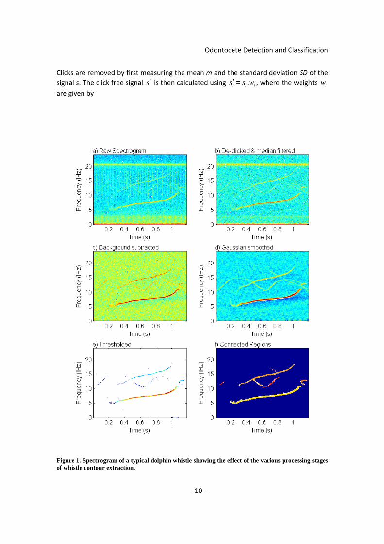
Figure 1. Spectrogram of a typical dolphin whistle showing the effect of the various processing stages of whistle contour extraction.

Odontocete Detection and Classification
- 11 -
( )
×−+
=power
i
i
SDthresh
msw
1
1
Where thresh is a threshold (default value 5) and power is an even power factor (default
value 6).
For small signals, where s – m << thresh, the weighting factor w is very close to 1.0 and
therefore has little effect on the signal. For large signals (such as within an echolocation
click), s – m>>thresh and w becomes very small, thereby reducing the signal.
5.1.2. Spectrogram calculation
Once blocks of data have been de-clicked, the FFT of those data is calculated using a
standard FFT algorithm in PAMGUARD. As part of our efforts to increase computation
speed during the development of the Whistle and Moan detector an algorithm written
by the PAMGUARD team was replaced by one in a newly available open source library
jtransforms1.
5.1.3. Spectrogram noise Removal
Three noise removal algorithms are applied to the spectrogram data.
Median filter
The median filter is used to enhance tonal peaks in the spectrogram by effectively
flattening the spectrum across the entire frequency range. It is also effective at
removing broad band clicks. It examines a single slice of FFT data at a time. For each
point in the FFT data, 61 points are taken around that point (i.e. 30 either side) and the
median value of those 61 points is found. This median value is then subtracted from the
original data. The median value is used in preference to the mean, since this gives a
more robust measure of the central tendency of a distribution of skewed data.
If fy is the spectrum data at frequency bin f, and fly is the spectrum data on a decibel
scale, i.e. )(10log.10 ff yly = , then the data at the output of this noise reduction stage,
fyl ′ are calculated using
):( 3030 +−−=′ ffff lylymedianlyyl
Whereas a mean value subtraction could give a heavily distorted value due to a small
number of outliers (e.g. a few bins of high intensity due to the presence of whistle), the
median value gives a stable value for the central tendency, or a typical value of the
spectral intensity around each point.
The effect of the click removal and median filter can be seen in the spectrogram images
in Figure 1 a and 1 b.
1 http://sourceforge.net/projects/jtransforms/

Odontocete Detection and Classification
- 12 -
Average Subtraction
To remove constant tones from the spectrogram, a running average background ftb , is
calculated at each time and frequency using
( ) ftftft blyb ,1,, .1. −−+= αα , where α is a small number (default 0.02).
This is then subtracted from the output of the median filter to give
ftftft bylyl ,1,, −−′=′′
The effect of this noise reduction stage is clearly visible in Figure 1 c where the constant
tone at 20kHz has been removed from the spectrogram.
Gaussian Smoothing Kernel
The spectrogram is them smoothed by convolving it with a gaussian smoothing kernel to
compute the smoothed spectrogram
Gyy ∗′′=′′′ , where
=121
242
121
G .
The effect of this operation can be seen in Figure 1 d. Although subtle, the amplitude of
the less intense whistle at around 15kHz has become more stable, thereby making the
whistle less likely to break into multiple parts. The Gaussian smoothing also removes
large number of single pixel regions from the final stage. Although never detected as
whistles, large numbers of single pixels in the final stage of the algorithm greatly
increase processing times.
5.1.4. Thresholding
After the Gaussian smoothing of the spectrogram a threshold is applied, all data points
in the spectrogram below that threshold are set to 0. The default value in PAMGUARD is
set to 8dB. The effect of thresholding can be seen in Figure 1 e.
5.1.5. Connecting Regions
Following thresholding, we are left with what is effectively a binary map of points which
were above threshold and points which were below threshold. The next stage of the
process is to connect these into regions a region being made up of pixels in the
spectrogram which are in direct contact with one another. Two types of connection
contact are defined, connect-8 and connect-4. If connect-8 (the PAMGUARD default) is
used, then spectrogram pixels are counted as in contact if they touch on their corners as
well as their sides. If connect-4 is used, then only side to side, or top to bottom contact
between pixels is allowed. Finally, small regions containing less than a minimum number
of pixels (PAMGUARD default 20) or which are shorter than a minimum total length in
Odontocete Detection and Classification
- 13 -
time (PAMGUARD default 10 time bins) are discarded. The example in Figure 1e shows a
total of 7 regions.
5.1.6. Crossing, Merging and Branching Regions
It can be seen in Figure 1e that the long whistle at around 15 kHz appears to split into
two branches at about 0.5 seconds. This is clearly due to a different, lower amplitude
whistle crossing the main whistle, although most of that other whistle was not detected.
Whistles of different amplitude crossing in this way is not at all uncommon when large
groups of dolphins are encountered. Although not necessarily a problem for the primary
task of detecting that dolphins are present, the whistle classifier (Section 0) will not
work well with poorly defined or confused contours. A set of rules have been developed
to break whistles at branches, crosses or joins (collectively referred to as nodes) and to
then optionally rejoin whistles across these nodes.
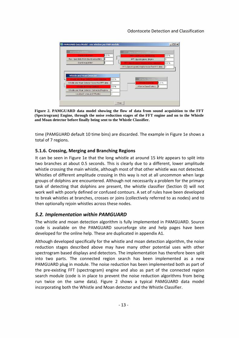
5.2. Implementation within PAMGUARD
The whistle and moan detection algorithm is fully implemented in PAMGUARD. Source
code is available on the PAMGUARD sourceforge site and help pages have been
developed for the online help. These are duplicated in appendix A1.
Although developed specifically for the whistle and moan detection algorithm, the noise
reduction stages described above may have many other potential uses with other
spectrogram based displays and detectors. The implementation has therefore been split
into two parts. The connected region search has been implemented as a new
PAMGUARD plug in module. The noise reduction has been implemented both as part of
the pre-existing FFT (spectrogram) engine and also as part of the connected region
search module (code is in place to prevent the noise reduction algorithms from being
run twice on the same data). Figure 2 shows a typical PAMGUARD data model
incorporating both the Whistle and Moan detector and the Whistle Classifier.
Figure 2. PAMGUARD data model showing the flow of data from sound acquisition to the FFT (Spectrogram) Engine, through the noise reduction stages of the FFT engine and on to the Whistle and Moan detector before finally being sent to the Whistle Classifier.

Odontocete Detection and Classification
- 14 -
5.2.1. Localisation
Spectrogram data, in its basic form is made up of complex numbers (that is numbers
which have a real part and an imaginary part). The complex spectrogram data conveys
the phase of the signal at any one time and frequency as well as it’s amplitude. While all
of the spectrogram noise reduction stages described above only require the amplitude
of the spectrogram at any point, the phase data is important in the estimation of
bearings to whistles and is retained throughout the contour extraction processes.
A cross correlation of whistle contour data from two hydrophone channels will give a
measure of the time delay between the arrival of the signal on each channel. If only two
channels are used, then a single bearing is returned, which will be subject to left/right,
or rotational ambiguity about the array axis. If more hydrophones are used in a planar
or volumetric array, then unambiguous bearings will be calculated. With the current
algorithm, bearing calculations are only possible with closely spaced hydrophones. By
closely spaced we mean that the maximum delay, measured in samples, between the
signal arrival on different channels must be less than half the length of the FFT used in
the spectrogram calculation process. For instance, if the data were sampled at 48 kHz
and an FFT length of 512 points were used, then the maximum delay between channels
can be no more than 256 samples or 5.3ms, which equates to an absolute maximum of
an 8m hydrophone separation.
Two forms of localisation are available, depending on array configuration. If a single
group of two or more hydrophones is used, then a bearing is calculated and no range
data is available. If hydrophones are arranged into two or more groups, with two or
more hydrophones per group, then ranges will be calculated by crossing bearings from
each group of hydrophones. For example, a four channel hydrophone array with two
pairs of hydrophones was used during the Gulf of Mexico PAMGUARD trial in 2008
(Douglas Gillespie 2009). Each pair had a spacing of 25cm so that bearings from the pair
could be calculated. The distance between pairs was 250m. Unfortunately, during that
trial, no whistles were detected, but we have discussed the use of similar arrays with
PAM service providers. Details on how to configure the Whistle and Moan detector for
different types of localisation are given in the online help (see Appendix A).
5.2.2. Database Output
The times and frequency ranges of detected whistle contours are written to the
PAMGUARD database if a database module has been loaded. Complete whistle contour
information is output to the PAMGUARD binary store.
5.3. Use with Baleen Whales
Preliminary tests have indicated that the whistle and moan detector is good at detecting
baleen whale calls. Figure 3 shows 30 seconds of data containing both fin whale and
North Atlantic right whale sounds processed with PAMGUARD. Sounds of both species
are clearly detected. However, it is very likely that the detector would also pick up low
frequency noise, so for it to become genuinely useful for use with baleen whales an

Odontocete Detection and Classification
- 15 -
additional module would be required to further analyse the detector output, reject
noise and classify calls to species. This would be something similar to the statistical
classifier built into the Right Whale Detection buoys deployed off the US east coast, the
algorithm for which is described in D. Gillespie 2004.
6. Whistle Classification
A significant problem when detecting and classifying whistles is that single whistles are
often broken during the detection process, appearing within the analysis software as
two or more separate whistles. When developing automatic detectors, such as the one
described in section 5 above, there is an inevitable trade off between allowing such
segmented whistles to join (as they should) and causing the detector to join together
segments of noise or different whistles (as they shouldn’t). Some whistle classifiers (e.g.
ROCCA, Oswald et al. 2007) avoid this problem by using a human operator to manually
select clearly visible whistles which are unbroken and have a high signal to noise ratio.
The software has to then only find the loudest whistle contour within that range of time
and frequency, generally working with the premise that there is exactly one whistle
Figure 3. Baleen whale detection using the Whistle and Moan detector. The 30s of data contain a downsweep from a fin whale at approx. 4s and a number of upsweeps from North Atlantic Right Whales between 17 and 24s. The top plot shows the unprocessed spectrogram, the middle plot the spectrogram after noise reduction and thresholding and the bottom plot shows detector output overlaid on the spectrogram.

Odontocete Detection and Classification
- 16 -
present, which is a considerably easier problem than detecting when you don’t know if a
whistle is there or not.
Our intention was to develop a classifier which could work with fully automatic detector
output, which therefore requires that the classifier be able to work with segmented
whistle contour data. Since the level of segmentation of whistles is heavily dependent
on factors such as the rate of click production, the number of overlapping whistles (a
function of species and group size) and other environmental noise, our approach has
been to further fragment the detected whistle segments so that they are of uniform
size. Since the individual fragments do not contain sufficient information for
classification, a number (several 10’s or 100’s) of fragments are accumulated over time
and a statistical analysis of multiple fragments is used to provide a species classification
for those many fragments. Since dolphin species are often encountered in groups and
produce many whistles during the course of a typical encounter, species identification at
the group rather than the individual level can be achieved.
Terminology:
Whistle – a complete whistle contour, as produced by the animal
Segment – a section of a whistle as found by a detector. A single whistle may produce
one or more separate segments.
Fragment – a small part of a whistle segment which has been further broken up during
the analysis process.
Section – a series of fragments accumulated over time.
The methods have been developed to work with output from either the PAMGUARD
Whistle Detector, which was implemented in PAMGUARD in 2006 or with the new
Whistle and Moan detector which was developed as part of this project (section 5).
6.1. Methods
6.1.1. Fragmentation
All detected whistle segments are broken into fragments of equal length. The number of
fragments per segment will naturally depend on the fragment and segment lengths.
Fragment start points within a whistle are set according to the following rules:
• If the segment length is shorter than the fragment length, no fragments are
created.
• If the segment length is an exact multiple of the fragment length, then there is
no overlap between fragments and the number of fragments is equal to the
segment length divided by the fragment length.
• If the segment length is not an exact multiple of the fragment length, then the
number of fragments is set to one more than the number of non-overlapping
fragments which could be made from the segment. These fragments are then

Odontocete Detection and Classification
- 17 -
distributed evenly along the length of the segment, ensuring that the first and
last points in the segment are included in the first and last fragments
respectively.
6.1.2. Statistical Parameter Extraction
Once fragments have been created, three parameters are extracted from each
fragment. These are
1. The mean frequency (Hz)
2. The slope of the frequency change over time (Hz/s)
3. The curvature of the fragment, which is measured using a second order
polynomial fit to the fragment contour, returning a curvature in Hz/s2.
Distributions of these three parameters for four example species (bottlenose dolphin,
common Dolphin, killer whales and Risso’s dolphin are shown in Figure 4. Examining
these distributions by eye, it is clear that it would not be possible to separate these
species based on these parameters alone. However, while the distributions clearly
Figure 4. Parameter distributions for the mean, slope and curvature of whistle fragments for three UK species.
0 10 200
500
1000BD - Mean
n=14389
-20 0 200
1000
2000BD - Slope
n=14389
-50 0 500
1000
2000
3000BD - Curve
n=14389
0 10 200
2000
4000CD - Mean
n=58446
-20 0 200
5000
10000CD - Slope
n=58446
-50 0 500
5000
10000
15000CD - Curve
n=58446
0 10 200
500
1000KW - Mean
n=12022
-20 0 200
2000
4000
6000KW - Slope
n=12022
-50 0 500
2000
4000
6000KW - Curve
n=12022
0 10 200
500
1000
1500RD - Mean
n=18803
-20 0 200
2000
4000RD - Slope
n=18803
-50 0 500
2000
4000
6000RD - Curve
n=18803

Odontocete Detection and Classification
- 18 -
overlap, they also have markedly different shapes. For instance, while the slopes of the
fragments are all broadly similar, the widths of each distribution are very different.
Therefore by accumulating parameters such as these over many fragments and building
up distributions of those parameters, it becomes possible to build a secondary set of
parameters which no longer describe individual whistle fragments, but instead describe
the distributions of parameters accumulated over time. From the distribution of each of
the three parameters, three parameters are extracted. These are the mean, the
standard deviation (or width) of each distribution and the skew (or lopsidedness) of
each distribution. This yields a total of 9 parameters describing a set of accumulated
whistle fragments. Distributions of these parameters for the same data shown in Figure
4 are presented in Figure 5.

Odontocete Detection and Classification
- 19 -
It can be seen from Figure 5 that the distributions of parameters from each species are
now noticeably different. For example, the distribution of “Slope STD” for killer whales is
at lower values than the corresponding parameters for the other species. This is a direct
Fig
ure
5. P
aram
eter
s de
scrib
ing
the
dist
ribut
ions
of pa
ram
eter
s fr
om a
ccum
ulat
ions
of 5
0 w
hist
le fr
agme
nts.

Odontocete Detection and Classification
- 20 -
reflection of the narrowness of the distribution of slope values for this species in Figure
4.
1.1.1. Classification
The nine parameters derived from the distributions of the three original parameters are
used in a linear discriminant classifier to determine species2.
Classifier Training and Testing
As is normal when training and testing a statistical classifier two thirds of the data were
used to train the classifier and one third of the data to test the classifier. Training and
testing were conducted multiple times using different sub sets of the data to asses
variability in the classifier performance. If each data point were fully independent of
other data points, then the normal way to select training and test data would be to
make a fully random selection of training data and then to use what’s left for testing.
With dolphin whistles however, there is a high probability that data collected during the
same recording session will be more similar than those collected at a different time and
place. Fully randomising the data with therefore tend to give a better and more stable
classification results than if the classifier were trained using data from one recording
session and tested with data from a different time and place. I.e. if we were to take data
from two recording sessions, A and B, a mixture of A and B will be quite similar to a
different mixture of A and B, whereas pure A will be more likely to be different to pure
B.
Ideally therefore, we would ensure that our data were tested and trained using only
data from different recording sessions. With the data available though, this was not
possible, since for some species, most of our whistle data came from a very small
number of very long recording sessions. We therefore adopted a policy whereby the
data for each species were laid out sequentially. A random start point in the sequence
was chosen and 2/3 of the data from that point selected for training (looping back to the
2 We are investigating alternative classifiers such as regression trees and random forests.
Table 2. Example confusion matrix from a single bootstrap
Classification Result (%)
BD CD KW RD Total
Tru
e S
pec
ies
BD 95 2 1 2 100
CD 18 56 0 26 100
KW 0 2 98 0 100
RD 1 2 1 96 100
Total 114 62 100 124

Odontocete Detection and Classification
- 21 -
start of the data once the end had been reached). Test data would then be the
remaining third of the data following on from wherever the training data ended.
To test the stability of the classification training, the data can be bootstapped many
times using different selection starting points for each bootstrap.
Classifier Training Output
When training the classifier, the output of each training step is a confusion matrix which
is derived from the test portion of the data. The confusion matrix shows how sections of
data from each species were classified. An example is shown in Table 2. Each row of the
table shows us how each species was classified. For example, bottlenose dolphins were
correctly classified 95% of the time, with the other five percent being misclassified. Only
56% of common dolphin sections were correctly classified, with 18 percent being
classified as bottlenose dolphin, and 26 percent being classified as Rissos. Each species
must be classified as something, so the sum of each row is always 100%, however,
misclassification between species results in the sums of each column varying. The
confusion matrix in Table 2 results from a single training selection and a single test
selection. Almost as important as the confusion matrix itself is how much the confusion
between species varies. This variation is estimated by repeating the training and testing
of data multiple times using different subsets of the available data (bootstrapping). By
repeating the bootstrap process many times, it is possible to not only measure the mean
confusion, but also the standard deviation and upper and lower confidence intervals for
each value. Table 3 shows the mean confusion matrix from 100 bootstraps along with
the standard deviation for the correct classification results. It can now been seen that
the 95% successful classification from the training in Table 2 was largely down to luck,
the true value being 65% +/- 21%.
Classifier optimisation
Two key parameters to select when setting up a classifier of this type are the length of
each fragment and the number of fragments to accumulate in each section before a
classification takes place. Longer fragment lengths and long sections should be expected
to lead to more stable classifiers, however if fragment lengths or sections are too long
Table 3. Mean and standard deviation confusion matrix after 100 bootstraps
Classification result (+/- Standard Deviation) %
BD CD KW RD
Tru
e S
pec
ies BD 65 (21) 25 (17) 1 (0) 8 (4)
CD 6 (6) 74 (12) 0 (0) 18 (7)
KW 0 (0) 0 (0) 99 (0) 0 (0)
RD 5 (5) 11 (9) 2 (3) 79 (17)

Odontocete Detection and Classification
- 22 -
then not enough data may be collected to allow classification to take place at all. The
classifier was therefore tested with varying fragment and section lengths to examine
these effects in detail.
6.2. Implementation in PAMGUARD
The whistle classifier is fully implemented in PAMGUARD. The source code is available
on the PAMGUARD sourceforge website, and help pages have been developed for the
online PAMGUARD help system. These are recreated in appendix 2.
6.2.1. Classifier Training
One of the most significant features of the PAMGUARD implementation is that
operators can train the classifier with their own samples of data. This is essential since
the small number of species with which we were able to train classifiers are all from the
North Atlantic and Gulf of Mexico. There is now good evidence that whistle
characteristics of a single species can be quite different within separate populations, so
our classifier trainings are of little use to those working in other parts of the world, even
in the unlikely event that they are working the same species as we are.
To train the classifier, a user must first accumulate recordings of species of interest to
them. They then process the recordings with the whistle and moan detector to generate
files of whistle contours. The classifier training is then run on the contour files and the
parameters derived from the training stored for future use processing additional data,
either from file or in real time.
Full details and instructions of the classifier training process are available in the
PAMGUARD online help (Appendix 2).
Table 4. Numbers of detected contours and numbers of fragments (fragment length 20 FFT bins)
Number of contours Number of 20 bin fragments
Average fragments
per contour >= 10 bins >= 20 bins BD 14322 5609 14389 2.6 BEL 2367 441 890 2.0 CD 51554 23130 58446 2.5 DUSK 1276 509 1459 2.9 FKW 11838 7271 22217 3.1 FRA 1758 802 2372 3.0 KW 12088 4873 12022 2.5 LPLT 5655 2217 5340 2.4 PKW 254 96 260 2.7 PLT 12700 4794 11580 2.4 RD 20136 8053 18803 2.3 SPIN 3079 1746 5269 3.0 SPT 34943 12539 29335 2.3 STR 27014 12321 33060 2.7 WBD 523 223 594 2.7 WSD 19919 7739 17965 2.3
Odontocete Detection and Classification
- 23 -
1.1.2. Classifier Operation
As with classifier training, full details and instructions are given in online help. The user
is presented with a display of the populating histograms of extracted fragment
parameters and also a time series display of classification results. Classification results
are also written to the PAMGUARD database if a database module is present in the
configuration.
7. Whistle Detection and Classification Results
7.1. Detection
All data described in section 4 were processed with the whistle and moan detector to
detect contours. The numbers of contours for each species are shown in Table 4.
7.2. Classification
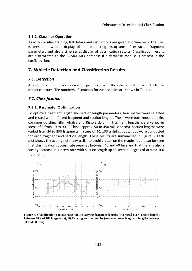
7.2.1. Parameter Optimisation
To optimise fragment length and section length parameters, four species were selected
and tested with different fragment and section lengths. These were bottlenose dolphin,
common dolphin, killer whales and Risso’s dolphin. Fragment lengths were varied in
steps of 2 from 10 to 90 FFT bins (approx. 50 to 450 milliseconds). Section lengths were
varied from 20 to 200 fragments in steps of 20. 100 training bootstraps were conducted
for each fragment and section length. These results are summarised in Figure 6. Each
plot shows the average of many trails, to avoid clutter on the graphs, but it can be seen
that classification success rate peaks at between 40 and 60 bins and that there is also a
steady increase in success rate with section length up to section lengths of around 100
fragments
Figure 6. Classification success rates for A) varying fragment lengths (averaged over section lengths between 40 and 100 fragments); B) Varying section lengths (averaged over fragment lengths between 30 and 50 bins).
0 10 20 30 40 50 60 70 80 900.5
0.6
0.7
0.8
0.9
1
Fragment Length
Mea
n co
rrec
t cl
assi
ficat
ion
rate
A)
0 50 100 150 2000.5
0.6
0.7
0.8
0.9
1
Section Length
Mea
n co
rrec
t cl
assi
ficat
ion
rate
B)

Odontocete Detection and Classification
- 24 -
7.2.2. Testing with species groups
Realistically, training the classifier to distinguish all 17 species at once is little more than
an academic exercise since several of the species in the training data set are extremely
unlikely to be found in the same area. The task of classification is considerably simplified
if the classifier is trained only with species encountered in an area of interest. Table 5
Table 5. Species grouping by region. An X denotes that the species is likely to occur in that area.
Polar Atlantic
Atlantic Frontier
Gulf of Mexico
Tropical Atlantic
Bottlenose Dolphin
BD X X X
Beluga Whale BEL X
Common Dolphin
CD X X
Dusky Dolphin
DUSK
False Killer Whale
FKW X X X
Fraser's Dolphin
FRA X X
Killer Whale KW X X X
Long Finned Pilot Whale
LPLT X X X X
Pigmy Killer Whale
PKW X X
Pilot Whale (Unidentified)
PLT
Risso's Dolphin RD X X X
Spinner Dolphin SPIN X X
Short Finned Pilot Whale SPLT X X
Spotted Dolphin
SPT X X
Striped Dolphin
STR X X
White-beaked Dolphin
WBD X X
White Sided Dolphin
WSD X X
Number of Species
4 8 11 12

Odontocete Detection and Classification
- 25 -
shows the known presence of the different species in four areas of interest. Numbers of
species in each region vary between four and twelve.
Contours were therefore divided up and processed by region. There were insufficient
pigmy killer whale data for training so that species was excluded. Additionally, it is highly
likely, based on recording locations, that the unknown pilot whale recordings were of
short finned pilot whales, so short finned and unknown pilot whales were grouped
together.
It was found that training with fragment length of 40 and a section length of 100 was
not possible for all species due to a lack of data. Classifier training was therefore
conducted with a fragment length of 30 and a section length of 60, which would be
expected to give slightly less than optimal results
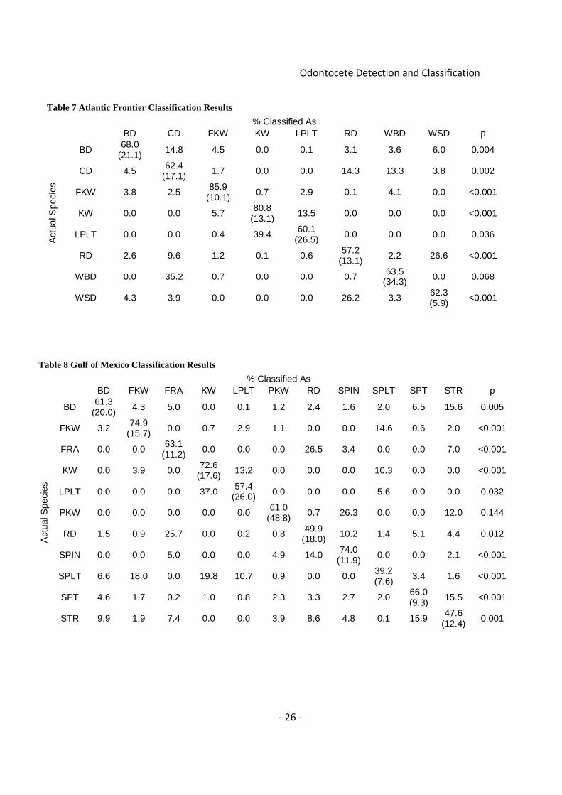
Results for the four regions are shown in tables 6 to 9. Each set of results is presented by
a confusion matrix which shows how each species would have been classified. The final
column in each table shows the probability of the result being purely due to chance. It
can be seen that for all but White Beaked dolphin on the Atlantic Frontier and pigmy
killer whales, all results are highly significant.
The reality is of course that the classifier is not 100% perfect. A summary of all regions is
shown in table 10. The best region is the polar Atlantic which achieves an average 94.5%
correct classification for four species. With larger numbers of species, the correct
classification rate drops to between 58 and 67%.
Table 6 Polar Atlantic Classification Results
% Classified As BEL LPLT WBD WSD P
Act
ual S
peci
es BEL 92.3
(19.4) 6.5 1.2 0.0 <0.001
LPLT 2.6 97.4 (4.2)
0.0 0.0 <0.001
WBD 0.0 0.0 93.3 (19.7)
6.7 <0.001
WSD 0.3 0.0 4.7 95.0 (3.3)
<0.001
Odontocete Detection and Classification
- 26 -
Table 7 Atlantic Frontier Classification Results
% Classified As BD CD FKW KW LPLT RD WBD WSD p
Act
ual S
peci
es
BD 68.0
(21.1) 14.8 4.5 0.0 0.1 3.1 3.6 6.0 0.004
CD 4.5 62.4
(17.1) 1.7 0.0 0.0 14.3 13.3 3.8 0.002
FKW 3.8 2.5 85.9
(10.1) 0.7 2.9 0.1 4.1 0.0 <0.001
KW 0.0 0.0 5.7 80.8
(13.1) 13.5 0.0 0.0 0.0 <0.001
LPLT 0.0 0.0 0.4 39.4 60.1
(26.5) 0.0 0.0 0.0 0.036
RD 2.6 9.6 1.2 0.1 0.6 57.2
(13.1) 2.2 26.6 <0.001
WBD 0.0 35.2 0.7 0.0 0.0 0.7 63.5 (34.3) 0.0 0.068
WSD 4.3 3.9 0.0 0.0 0.0 26.2 3.3 62.3 (5.9)
<0.001
Table 8 Gulf of Mexico Classification Results
% Classified As BD FKW FRA KW LPLT PKW RD SPIN SPLT SPT STR p
Act
ual S
peci
es
BD 61.3
(20.0) 4.3 5.0 0.0 0.1 1.2 2.4 1.6 2.0 6.5 15.6 0.005
FKW 3.2 74.9
(15.7) 0.0 0.7 2.9 1.1 0.0 0.0 14.6 0.6 2.0 <0.001
FRA 0.0 0.0 63.1
(11.2) 0.0 0.0 0.0 26.5 3.4 0.0 0.0 7.0 <0.001
KW 0.0 3.9 0.0 72.6
(17.6) 13.2 0.0 0.0 0.0 10.3 0.0 0.0 <0.001
LPLT 0.0 0.0 0.0 37.0 57.4
(26.0) 0.0 0.0 0.0 5.6 0.0 0.0 0.032
PKW 0.0 0.0 0.0 0.0 0.0 61.0 (48.8)
0.7 26.3 0.0 0.0 12.0 0.144
RD 1.5 0.9 25.7 0.0 0.2 0.8 49.9 (18.0)
10.2 1.4 5.1 4.4 0.012
SPIN 0.0 0.0 5.0 0.0 0.0 4.9 14.0 74.0 (11.9)
0.0 0.0 2.1 <0.001
SPLT 6.6 18.0 0.0 19.8 10.7 0.9 0.0 0.0 39.2 (7.6)
3.4 1.6 <0.001
SPT 4.6 1.7 0.2 1.0 0.8 2.3 3.3 2.7 2.0 66.0 (9.3)
15.5 <0.001
STR 9.9 1.9 7.4 0.0 0.0 3.9 8.6 4.8 0.1 15.9 47.6
(12.4) 0.001

Odontocete Detection and Classification
- 27 -
8. Click Classification
A new click classification system has been developed and implemented in PAMGUARD.
The purpose of the click classifier is to identify individual clicks to species level. The
priority species for this work were beaked whales since a) beaked whales have been
know to strand in response to the use of military sonar (Frantzis 1998; Evans et al. 2001;
Cox et al. 2005) and may be generally susceptible to adverse affects resulting from
anthropogenic sound and b) beaked whales do not (to the best of our knowledge)
Table 9 Tropical Atlantic Classification Results
% Classified As BD CD FKW FRA KW LPLT PKW RD SPIN SPLT SPT STR p
Act
ual S
peci
es
BD 64.3
(20.1) 8.7 3.5 4.3 0.0 0.1 0.4 1.3 1.1 1.4 6.1 8.8 0.003
CD 4.0 53.9
(15.8) 1.7 4.9 0.0 0.0 3.4 8.4 10.0 0.2 1.0 12.7 0.002
FKW 3.6 2.6 72.1
(16.3) 0.0 0.9 3.7 1.0 0.0 0.0 14.1 0.7 1.2 <0.001
FRA 0.0 8.5 0.0 59.8
(11.7) 0.0 0.0 0.0 22.3 2.6 0.0 0.0 6.9 <0.001
KW 0.0 0.0 3.8 0.0 72.6
(18.0) 12.8 0.1 0.0 0.0 10.7 0.0 0.0 <0.001
LPLT 0.0 0.0 0.0 0.0 37.9 55.2
(25.5) 0.0 0.0 0.0 6.9 0.0 0.0 0.033
PKW 0.0 17.0 0.0 0.0 0.0 0.0 60.3 (48.9) 0.0 22.7 0.0 0.0 0.0 0.144
RD 1.0 5.4 0.6 25.1 0.0 0.1 0.9 49.4 (17.9)
9.4 1.2 4.4 2.7 0.011
SPIN 0.0 11.7 0.0 2.5 0.0 0.0 2.7 10.3 72.6 (12.0)
0.0 0.0 0.3 <0.001
SPLT 7.1 1.1 17.1 0.0 17.8 10.3 0.5 0.0 0.0 41.1 (7.5) 3.6 1.4 <0.001
SPT 4.6 1.4 1.4 0.1 0.9 0.7 2.1 3.2 1.6 1.8 68.4 (9.1)
14.0 <0.001
STR 9.7 19.4 1.7 4.9 0.0 0.0 3.6 6.0 3.7 0.1 16.8 34.1 (9.1)
0.002
Table 10. Summary of classification results by region.
Region Number of Species
Mean Correct Classification Rate
Polar Atlantic 4 94.5
Atlantic Frontier 8 67.5
Gulf of Mexico 11 60.6
Tropical Atlantic 12 58.6

Odontocete Detection and Classification
- 28 -
whistle and cannot therefore be detected or classified using the whistle detection and
classification methods described above.
Beaked whales are an unusually diverse group with 21 genetically confirmed species
(Dalebout et al. 2004). Wide bandwidth recordings have been made and reported from
only a handful of species however. Recent work using recording tags (DTAG – (M. P.
Johnson & Tyack 2003) attached to individual whales using suction cups, have provided
extremely detailed information on the acoustic characteristics of the sounds produced
by two species: Cuviers and Blainville’s beaked whales (Johnson et al. 2004; Madsen et
al. 2005; Zimmer et al. 2005, Johnson et al. 2006).
The dominant energy in Cuvier’s beaked whale clicks was shown to be between 30 and
45 kHz and click lengths were around 200 µs (micro seconds). The clicks of Blainville’s
beaked whales were broadly similar to those of the Cuvier’s. The recording bandwidth
of the tag used in some of the earlier studies was 48 kHz, leading to speculation that
there may be energy at even higher frequencies. However, later work using DTAGs with
sampling rates of 192 kHz and a cabled hydrophone system with sensitivity up to 180
kHz ((Zimmer, M. P. Johnson, et al. 2005c) have confirmed that the dominant frequency
for Cuvier’s beaked whales is indeed in the 30 – 40 kHz region.
By combining tracking data and recordings from DTAGs on two Cuvier’s beaked whales
tagged concurrently, Zimmer et al. (2005) were able to calculate a peak to peak source
level for clicks of 214 dB re: 1 µPa at 1 m, and a directionality index of 25dB.
Clicks of similar frequency have also been recorded from other beaked whale species
including Baird’s beaked whale (Berardius bairdii), which had frequency peaks between
23 kHz and 42 kHz (Dawson, Barlow, et al. 1998a) and northern bottlenose whales
(Hyperoodon ampullatus) which had frequency peaks at a mean frequency of 24 kHz
while foraging (Hooker & Whitehead 2002). Analysing recordings from a towed
hydrophone array, Gillespie et al. 2009 reported similar clicks from Gervais beaked
whale (Mesoplodon europaeus) encountered in the Bahamas. Other species, such as
Sowerby's beaked whale (Mesoplodon bidens) have never been recorded.
The 25-40kHz frequency range used by beaked whales is also utilised by many other
small cetacean species. Unfortunately, until relatively recently, accessible field recording
equipment used by field biologists often only recorded up to around 20kHz resulting in
many species only being reported as vocalising at lower frequencies. As wide band
recording systems become more widely available, we are still learning about the high
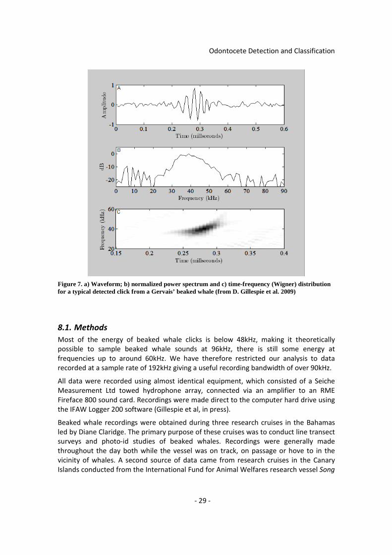
frequency behaviour of several species. One feature of beaked whale clicks which does
however seem to be common to several beaked whale species is the frequency
modulation of the clicks which tend to sweep up by several kHz as can be seen for the
Gervais beaked whale click shown in Figure 7. So far as is currently known, this upsweep
is a feature only found in beaked whale vocalisation.
Odontocete Detection and Classification
- 29 -
8.1. Methods
Most of the energy of beaked whale clicks is below 48kHz, making it theoretically
possible to sample beaked whale sounds at 96kHz, there is still some energy at
frequencies up to around 60kHz. We have therefore restricted our analysis to data
recorded at a sample rate of 192kHz giving a useful recording bandwidth of over 90kHz.
All data were recorded using almost identical equipment, which consisted of a Seiche
Measurement Ltd towed hydrophone array, connected via an amplifier to an RME
Fireface 800 sound card. Recordings were made direct to the computer hard drive using
the IFAW Logger 200 software (Gillespie et al, in press).
Beaked whale recordings were obtained during three research cruises in the Bahamas
led by Diane Claridge. The primary purpose of these cruises was to conduct line transect
surveys and photo-id studies of beaked whales. Recordings were generally made
throughout the day both while the vessel was on track, on passage or hove to in the
vicinity of whales. A second source of data came from research cruises in the Canary
Islands conducted from the International Fund for Animal Welfares research vessel Song
Figure 7. a) Waveform; b) normalized power spectrum and c) time-frequency (Wigner) distribution for a typical detected click from a Gervais’ beaked whale (from D. Gillespie et al. 2009)

Odontocete Detection and Classification
- 30 -
of the Whale. In both areas, both Blainvilles and Cuviers beaked whales were
encountered as well as a single encounter with Gervais beaked whale.
192kHZ sample rate recordings of noise and or other cetacean species were selected
from data collected during the Cetacean Offshore Distribution and Abundance (CODA)
line transect survey conducted by the Sea Mammal Research Unit in 2007. This covered
waters from the edge of the continental shelf to the 200 mile EEZ to the West of Britain,
France and the Iberian peninsular.
8.1.1. Data Selection
Recordings were first processed with the PAMGUARD click detector, set up to trigger in
the 25-40kHz band of interest. Data were output into a file format compatible with the
RainbowClick analysis software (D. Gillespie & Leaper 1996). These files were then
browsed by an operator who searched for trains of clicks, that is clicks appearing on a
consistent bearing with regular inter click intervals. Click trains from the CODA survey
were assigned to species through comparison with the visual sighting record. Beaked
whales do not vocalise at the surface, so in general, if you can hear a beaked whale, you
can’t see it and vice-versa. Beaked whale clicks were therefore selected primarily based
on the appearance of individual clicks and their similarity with waveforms and spectra in
published literature. Samples of noise from passing ships and also general background
noise – that is relatively low level clicks which caused a trigger, but were not associated
with an event such as a passing ship or animal.
Selected clicks were then extracted from the click files and imported into Matlab for
parameterisation and analysis.
Species available with data sampled at 192 kHz are
1. Beaked whales
2. Common dolphin
3. Bottlenose dolphin
4. Striped dolphin
8.1.2. Click Parameterisation
Parameters were extracted both from the click waveform and the clicks power
spectrum.
Parameters extracted from the click waveform and power spectrum are shown in Figure
9. These are
1. The click length
2. The number of zero crossings
3. The frequency sweep extracted from the zero crossing data
4. The energy in three different frequency bands

Odontocete Detection and Classification
- 31 -
5. The peak frequency
6. The mean frequency
Waveform Parameterisation
The first parameter extracted from the click waveform is it’s length. The envelope of the
waveform is calculated from the Hilbert transform of the wave data, the maximum
height is measured and a threshold set 8dB3 below that maximum. The envelope is then
smoothed using a five point moving average filter and the start and end of the click are
then taken as the points at which the envelope falls below that threshold before and
after the peak. The click length is then simply the time difference between the start and
3 All parameters such as length thresholds are adjustable by the user both in the Matlab code and in the final PAMGUARD release.
Figure 8. Parameterisation of a common dolphin click waveform and spectrum
Figure 9. Parameterisation of a beaked whale click waveform and spectrum
50 100 150 200-1000
-500
0
500
1000
1500
Time (samples)
Am
plitu
de
click waveform
waveform
envelope
smoothed envelopeclick limits
zero crossings
0 20 40 60 80 100-30
-25
-20
-15
-10
-5
0
Frequency (kHz)
Am
plitu
de (
dB)
Click spectrum
un smoothed
smoothedPeak Width
0 50 100 150 200-250
-200
-150
-100
-50
0
50
100
150
200
250
Time (samples)
Am
plitu
de
Click waveform
waveform
envelope
smoothed envelopeclick limits
zero crossings
0 20 40 60 80 100-30
-25
-20
-15
-10
-5
0
Frequency (kHz)
Am
plitu
de (
dB)
Click spectrum
un smoothed
smoothedPeak Width
Odontocete Detection and Classification
- 32 -
end times.
Once the start and end times have been determined, the zero crossing times are
extracted, these are the times at which the waveform crosses 0 amplitude. The time
between two successive zero crossings can be taken as an estimate of frequency at that
point, where the frequency f is given by
ZTf
2
1=
where Tz is the zero crossing interval.
If three or more zero crossings occur within the click, then there will be two or more
measures of frequency and it is then possible to calculate the frequency sweep from a
simple linear fit of frequency against time. If there are not enough zero crossing to
estimate frequency sweep, the sweep is set to zero.
Power spectrum parameterisation
The click power spectrum is calculated only in the vicinity of the waveform peak, in this
case using a 256 point FFT. As with the waveform envelope, the power spectrum is
smoothed using a moving average filter. Since the ocean noise is often dominant at low
frequencies, searches for the spectral peak and measurement of the mean frequency is
conducted only between 2 and 90 kHz (this can be varied in the PAMGUARD version
should there be differences in the noise background). The spectral peak width is also
estimated by finding the peak maximum and setting a threshold 8dB below that
maximum, then finding the regions of the spectrum above that threshold.
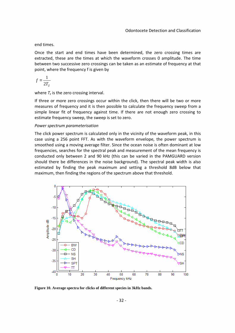
Figure 10. Average spectra for clicks of different species in 3kHz bands.

Odontocete Detection and Classification
- 33 -
In addition to these three parameters, the energy of each click in 3kHz bands was
measured relative to that in the highest band for each click.
Figure 11. Parameter distributions for the different species.

Odontocete Detection and Classification
- 34 -
Parameter distributions for the four cetacean species and two noise sources are shown
in Figure 10 and Figure 11.
8.1.3. Classification
From Figure 10 it can be seen that the frequency distributions of all four cetacean
species overlap heavily. While it is relatively straight forward to separate out the noise
based on measures of peak of mean frequency it would certainly not be possible to
separate beaked whales from the other cetacean species.
For the identification of beaked whales, the most outstanding parameters from Figure
11 are the numbers of zero crossings and the frequency sweep. There are no
parameters which show obvious differences between the three dolphin species.
While it would in principle be possible to
use the extracted parameters in a
multivariate classifier of the type used for
whistle classification, we have not done so
since the extraction of species training data
sets is reliant on software which is still
outside the PAMGUARD framework (i.e.
RainbowClick and a number of Matlab
scripts). This means that it would not
currently be practical for most PAMGUARD
users to develop and train their own
classifiers as can be done for the Whistle
classifier.
The click classification scheme implemented
in PAMGUARD uses a parameter selection
scheme which has the advantages of being
transparent to the users, fast in execution
Figure 12. Beaked Whale detection efficiency plotted against false alarm rate for dolphin clicks and noise clicks.
Figure 13. Click classification dialog. Here the user creates and deletes one or more classifiers for different species or noise types.
0 2 4 6 870
75
80
85
90
95
100
% dolphins detected as beaked whales
BW
effi
cien
cy (
%)
5 Zero Crossings6 Zero Crossings7 Zero Crossings8 Zero Crossings9 Zero Crossings10 Zero Crossings
0 0.2 0.4 0.6 0.870
75
80
85
90
95
100
% noise clicks detected as beaked whales
BW
effi
cien
cy (
%)
5 Zero Crossings6 Zero Crossings7 Zero Crossings8 Zero Crossings9 Zero Crossings10 Zero Crossings

Odontocete Detection and Classification
- 35 -
and relatively easy to tune for
additional species or noise
sources. The user sets up multiple
classifiers, one for each species or
noise source. For each classifier,
the user selects which parameters
they wish to use and then sets
upper and lower bounds to the
allowable values of each of those
parameters. A click is classified as
a particular type if it passes all the
selected tests. Classifiers are
processed one at a time. If a click
is given a positive classification by
any classifier, subsequent
classifiers are not tested. If a click
does not pass the tests of any
classifier, it remains unclassified.
8.2. Results
Beaked whale detection efficiency
is shown plotted against false alarm rate from dolphin clicks (average for common,
bottlenose and Risso’s dolphin) and from noise clicks (average for ship and random
noise) in Figure 12. Each line in each plot shows how efficiency and false alarm rate vary
as a function of minimum sweep rate for a minimum number of zero crossings. Each dot
represents the result of one sweep value, which varied from 0 to 30 kHz/ms in steps of
5. It can be seem that if the number of zero crossings is seven or over, then increasing
the sweep rate requirement has little effect on false alarm rate, but does reduce
detection efficiency.
8.3. Implementation in PAMGUARD
Classification is controlled using two dialogs accessible from the PAMGUARD menu
system. The first (Figure 13) is used to manage the different classifiers for multiple
species. Classifiers can be added or removed and it is possible to change their order. It is
also possible for clicks classified as a particular type to be immediately discarded. This
reduces display clutter from noise and can also improve overall PAMGUARD
performance and reduce output file sizes. The second dialog (Figure 14) is used to setup
parameters and display options for each individual classifier.
Each classifier is assigned a symbol shape and colour which are used on the click display
to easily distinguish clicks of different types.
While it is not possible for the classifier by itself to operate at zero false alarm rate,
there are a four displays built into the click detector which assist the operator in making
informed decisions about species identification. False alarms are most likely when large
Figure 14. Classifier options dialog showing typical beaked whale click detection settings.

Odontocete Detection and Classification
- 36 -
numbers of dolphin clicks or noise clicks are being received. The bearing time display
gives the operator an overview of all clicks received over a period of several minutes.
Figure 15 shows the bearing time display during a time with a beaked whale event and a
false detection due to dolphin clicks. The low numbers of non beaked whale clicks on
the left leads us to assume that these clicks are genuinely beaked whales, whereas the
high number of dolphin clicks and general noise on the right makes it clear that these
clicks are not.
The bearing time display is excellent for giving a quick overview of many clicks and how
they are formed into trains of clicks arriving from a consistent bearing, individual clicks
can be examined in detail using waveform, power spectrum and Wigner (time-
frequency) plots as shown in Figure 16.
All of these displays are available to the user both while analysing data in real time and
also when reviewing data offline. When reviewing data offline it is also possible to alter
the click classification parameters and to reprocess clicks stored using the PAMGUARD
binary storage system.
8.3.1. Online Help
The click classifier is fully documented in the PAMGUARD online help. The online help
pages are reproduced in Appendix 3.
9. Software Releases
A Beta version of the Whistle and Moan detector was first released in Version 1.7.00 in
October 2009. Bug fixes were applied to releases 1.8.00 Beta (January 2010) and 1.9.00
Beta (April 2010). The detector was integrated with the new binary data storage system
in Beta release 1.10.00 (December 2010).
The Whistle classifier was first released in version 1.7.00 Beta (October 2009) at the
same time as the new detector. Bug fixes were applied in version 1.9.00 Beta (April
2010).
Figure 15. Bearing time display showing (left) some brief beaked whale click trains and (right) false detections which occurred when several dolphins were passing the hydrophone.

Odontocete Detection and Classification
- 37 -
Both the new detector and the classifier were released in the Core version of
PAMGUARD v 1.10.00 in December 2010.
The new click classifier was released in version 1.8.00 Beta (January 2010) and also in
the 1.10.00 core release of December 2010.
10. Ongoing work and publications
A dataset of whistles from the Eastern Tropical Pacific has recently been released for
use at the 5th
Detection Classification and Localisation workshop, to be held in Oregon in
August 2011 (http://www.bioacoustics.us/dcl.html). The dataset has been processed
with the PAMGUARD whistle and moan detectors and the data have been used to train
the whistle classifier. These results will be presented at the workshop and it’s likely that
we will publish them in the workshop proceedings later in the year.
We are in the process of preparing a paper describing the click detection and
classification methods and their application to beaked whales. This will be submitted to
an appropriate journal in the spring of 2011.
11. References
Cox, T.M. et al., 2005. Understanding the impacts of anthropogenic sound on beaked
whales. Journal of Cetacean Research and Management, 7(3), p.177.
Figure 16. Waveform, Power spectrum and Wigner plots for a beaked whale click (top) and a false beaked whale detection (bottom).

Odontocete Detection and Classification
- 38 -
Dalebout, M.L. et al., 2004. A Comprehensive and Validated Molecular Taxonomy of
Beaked Whales, Family Ziphiidae. Journal of Heredity, 95(6), pp.459-473.
Dawson, S., Barlow, J. & Ljungblad, D., 1998a. Sounds Recorded From Baird’s Beaked
Whale, Berardius Bairdil. Marine Mammal Science, 14(2), pp.335-344.
Evans, D.L. et al., 2001. Joint Interim Report Bahamas Marine Mammal Stranding Event
of 15-16 March 2000. NOAA and Dept. of the Navy, 59.
Frantzis, A., 1998. Does acoustic testing strand whales? Nature, 392(6671), p.29.
Gillespie, D., 2004. Detection and classification of right whale calls using an edge
detector operating on a smoothed spectrogram. Canadian Acoustics, 32, pp.39-
47.
Gillespie, D. et al., 2009. Field recordings of Gervais’ beaked whales Mesoplodon
europaeus from the Bahamas. The Journal of the Acoustical Society of America,
125, p.3428.
Gillespie, D. & Leaper, R., 1996. Detection of sperm whale (Physeter macrocephalus)
clicks and discrimination of individual vocalisations. Eur. Res. Cetaceans, pp.87-
91.
Gillespie, Douglas, 2009. PAMGUARD Industry Field Trial 2008Final Report, St Andrews,
Scotland: SMRU Ltd.
Hooker, S.K. & Whitehead, H., 2002. Click characteristics of northern bottlenose whales
(hyperoodon ampullatus). Marine Mammal Science, 18(1), pp.69-80.
Johnson, M.P. & Tyack, P.L., 2003. A digital acoustic recording tag for measuring the
response of wild marine mammals to sound. Oceanic Engineering, IEEE Journal
of, 28(1), pp.3-12.
Oswald, J.N., Rankin, S., et al., 2007b. A tool for real-time acoustic species identification
of delphinid whistles. The Journal of the Acoustical Society of America, 122,
p.587.
Zimmer, W.M.X., Johnson, M.P., et al., 2005c. Echolocation clicks of free-ranging
Cuvier’s beaked whales (Ziphius cavirostris). The Journal of the Acoustical Society
of America, 117, pp.3919 - 3927.

Odontocete Detection and Classification
- 39 -
Appendix 1: Whistle and Moan Detector Help Pages
12. Whistle and Moan Detector
12.1. Overview
The Whistle and Moan detector can be used to detect any tonal vocalisation, including odontocete whistles and baleen whale calls.
The Whistle and Moan detector supersedes the old PAMGUARD Whistle detector which should no longer be used.
The Whistle and Moan detector can be used alone, or with the Whistle Classifier which can be used to identify groups of whistles to species.
12.1.1. Creating a Whistle and Moan detector
From the File>Add modules>Detectors menu, or from the pop-up menu on the data model display, select "Whistle and Tone Detector". Enter a descriptive name for the new detector (e.g. Whistle detector) and press OK.
12.1.2. General Principle of Detection
Detection is a multi-stage process, the main steps being
1. Computation of a spectrogram from raw audio data
2. Processing of the spectrogram to remove noise (especially clicks)
3. Thresholding to create a binary map of regions above threshold
4. Connecting regions of the binary map to create sounds
5. Breaking and then rejoining branches of complex regions (for instance, if two whistles cross)
Next: Configuring the Whistle and Moan Detector
12.2. Configuring the Whistle and Moan Detector
From the Detection menu select Whistle and Tone Detector and the following dialog will appear.

Odontocete Detection and Classification
- 40 -
The dialog contains two tabs, the first controls the Data source, Channel Grouping and How
sounds are connected. The second tab controls Noise removal and thresholding.
Previous: Whistle and Moan Detector Overview
Next: Configure the data source
12.3. Data Source Setup
To use the Whistle and Moan detector, you will need to configure a FFT (Spectrogram)
Engine. When selecting the FFT length and hop, consider the time and frequency resolution of the spectrogram. For instance, a 1024 pt FFT with 50% overlap (512 pt hop) operating on data with a sample rate of 48 kHz will have a frequency resolution of 47Hz and a time resolution of approximately 10ms. Generally, for detecting dolphin whistles with data sampled at 48 kHz, a 512 pt FFT length and 256 pt Hop is suitable. At higher sample rates, scale the FFT length and hop accordingly, i.e. at a sample rate of 96 kHz use a FFT length of 1024 pt and a hop of 512 pt, etc.
12.3.1. Select the data source
Noise removal and thresholding is a critical step in the detection process. However, the noise removal methods can also be used by other PAMGUARD detectors and displays, so they
The linked image cannot be displayed. The file may have been moved, renamed, or deleted. Verify that the link points to the correct file and location.

Odontocete Detection and Classification
- 41 -
have been included in both the FFT (Spectrogram) Engine as well as in the Whistle and Moan detector.
The FFT (Spectrogram) Engine has two output streams, one which is the raw FFT data and one which has been through some or all of the noise removal processes.
Whether you do the noise removal in the FFT Engine or in the Whistle and Moan detector is entirely up to you, but try not to do it twice since that will place an unnecessary load on the processor
From the drop down box at the top of the Whistle and Moan detector options dialog, select which data source you want to use.
Previous: Configure the Whistle and Moan Detector
Next: Configure channel grouping
12.4. Channel Grouping and Bearing Calculations
The Whistle and Moan detector can operate on one or more channels of data. It can also measure time delays between the arrival of sounds on different channels and use these to calculate bearings, and in some instances ranges to detected sounds.
The linked image cannot be displayed. The file may have been moved, renamed, or deleted. Verify that the link points to the correct file and location.
Odontocete Detection and Classification
- 42 -
Which channels the Whistle and Moan detector detects on and which channels it uses for bearing and range calculations is controlled by the channel grouping section of the options dialog.
When a data source is selected, the dialog will show a series of check boxes, one for each channel. Select the channels you want to use for detection OR bearing calculation, then to the right of each channel check box, assign the channel to a group. The group numbers themselves are not important - they just need to be different for each group.
The Whistle and Moan detector will detect sounds only on the first channel in each group.
If a sound is detected, it will then use data from other channels in the same group to measure time delays between the arrival of the signal on the different channels. The Whistle and Moan detector will do this independently for each group.
Measuring Range
If more than one group is present, then if whistles which overlap in time and frequency are detected on more than one channel group, the Whistle and Moan detector will attempt
The linked image cannot be displayed. The file may have been moved, renamed, or deleted. Verify that the link points to the correct file and location.

Odontocete Detection and Classification
- 43 -
to cross the bearings measured within each channel group in order to estimate a range to the sound.
The example above was set up to work with a hydrophone array which consisted of four hydrophones arranged in two pairs. The separation of each pair was 3m and the distance between pairs was 200m. Detection and bearing calculation was conducted independently from each pair, and the bearings from the two pairs then crossed to estimate ranges.
Previous: Configure the data source
Next: Configure the noise removal
12.5. Noise Removal and Thresholding
Noise removal and thresholding is one of the most important steps in the operation of the Whistle and Moan detector.
Noise removal and thresholding is a five stage process. The first stage has to occur before FFT data are calculated in the FFT (Spectrogram) Engine. The remaining four stages can take place either in the FFT (Spectrogram) Engine module or in the Whistle and Moan detector.
Performing the noise removal in the FFT (Spectrogram) Engine module has the advantage that other PAMGUARD processes and displays will have access to the data
The Whistle and Moan detector will try to ensure that the correct noise removal processes are run once and only once but looking back at the FFT data source and testing whether noise removal has already been done.
Noise removal processes which have already been conducted in an earlier module cannot be repeated. However, the Whistle and Moan detector cannot check, and has no control over the configuration of noise removal processes conducted in earlier modules.
Generally, you should use the default settings Click Removal Median Filter Average Subtraction Gaussian Kernel Smoothing Thresholding
12.5.1. Click Removal
This stage of the noise removal has to take place on the raw data prior to the calculation of the spectrogram. It is therefore carried out by the FFT (Spectrogram) Engine.
The click removal method operates on the time series data prior to the FFT calculation and therefore affects both output streams of the FFT Engine.
Odontocete Detection and Classification
- 44 -
Click removal measures the standard deviation of the time series data and then multiplies the signal by a factor which increases rapidly for large signal components. This has the effect of reducing the magnitude of short duration transient signals such as echolocation clicks
Other noise removal stages can be controlled from either the Whistle and Tine detector dialog or from the FFT (Spectrogram) Engine
The linked image cannot be displayed. The file may have been moved, renamed, or deleted. Verify that the link points to the correct file and location.

Odontocete Detection and Classification
- 45 -
12.5.2. Median Filter
Within each spectrogram slice, the median value about each point is taken and subtracted from that point.
12.5.3. Average Subtraction
A decaying average spectrogram is computed and subtracted from the current spectrogram value.
12.5.4. Gaussian Kernel Smoothing
The spectrogram is smoothed by convolving the image with a Gaussian smoothing kernel
1 2 1 2 4 2 1 2 1.
12.5.5. Thresholding
A threshold is applied and all data falling below that threshold set to 0.
Although the Connected Region Search uses only a binary map of parts of the spectrogram which are above or below threshold it is generally more useful to output the input from
The linked image cannot be displayed. The file may have been moved, renamed, or deleted. Verify that the link points to the correct file and location.

Odontocete Detection and Classification
- 46 -
the raw FFT data which will have been multiplied by the binary map. This will contain phase and amplitude information which can be used by the Whistle and Moan detector for measuring time delays between channels and the overall whistle amplitude.
Previous: Configure channel grouping
Next: Configure the region connector
12.6. Connected Region Search
Once the threshold has been applied to the spectrogram data in the noise removal stage, the Whistle and Moan detector searches for connected regions in the spectrogram matrix.
12.6.1. Min Frequency and Max Frequency
Usually, you will want the Whistle and Moan detector to search the whole range of available frequencies, from 0 Hz to half the sample rate. However, these parameters give you the opportunity to limit the connected region search to a specific frequency band. This can be particularly useful if your data are contaminated by a lot of noise at a particular frequency.
The linked image cannot be displayed. The file may have been moved, renamed, or deleted. Verify that the link points to the correct file and location.

Odontocete Detection and Classification
- 47 -
12.6.2. Connection Type
When searching for connected regions, two main connection types are available.
Connect 4 tries to connect each pixel to other pixels directly above, below, to the left or to the right (i.e. 4 possible connections).
Connect 8 tries to connect to the sides and on the diagonals (i.e. 8 possible connections).
Clearly connect 8 will detect more whistles and can also detect whistles sweeping more rapidly, however connect 8 may also be prone to a higher rate of false alarm if it connects things which shouldn't be connected.
12.6.3. Minimum length and Minimum total size
There will always be a small number of random spectrogram pixels which are above threshold but are not part of a whistle or tone. Generally (hopefully !) these will few in number and the chances of them connecting to other random pixels to make a large connected region will be small.
All connected regions which are shorter than the minimum length, or have fewer pixels than the minimum total size will be discarded.
Previous: Configure the noise removal
Next: Configure region branching
12.7. Branching and Joining
It is often the case that multiple whistles from different animals will overlap in time and frequency. If large groups of dolphins are encountered, then overlapping whistles tend to be the norm rather than the exception. While this may not be a problem if you are only interested in detecting whistles, if you are measuring bearings to individual whistles or if you are using the Whistle Classifier it is necessary to separate out the different sounds.
The Whistle and Moan detector has four options which control how overlapping whistles are handled
1. Leave branched regions intact
2. Discard branched regions
3. Separate all branches
4. Re-link across joins
This option is set at the bottom of the Whistle and Moan configuration dialog.

Odontocete Detection and Classification
- 48 -
The different options are illustrated below using three simulated overlapping linear chirps.
12.7.1. Leave branched regions intact
If this option is selected, then branched regions will be left intact and may contain more one actual sound.
The linked image cannot be displayed. The file may have been moved, renamed, or deleted. Verify that the link points to the correct file and location.
The linked image cannot be displayed. The file may have been moved, renamed, or deleted. Verify that the link points to the correct file and location.

Odontocete Detection and Classification
- 49 -
12.7.2. Discard branched joins
If this option is selected, than any region that has more than one detected frequency peak in any time slice will be discarded.
12.7.3. Separate all branches
If this option is selected, then all branches will be separated and passed on as individual sounds. A break is created every time the number of consecutive peaks changes. So a pair of crossing whistles will generally be broken into five parts - each of the four branches and the crossing point itself.
In the example below, the three sounds have been broken into 12 separate parts.
12.7.4. Re-link across joins
If this option is selected, then the algorithm will attempt to rejoin individual tones across joins. First, the sound is broken up as above, it then rejoins the different components according to the following rules:
1. If there are the same number of sounds in consecutive time slices and each sound in the earlier slice is in contact with one in the later slice, then they are joined with 1:1 correspondence.
2. A crossing point is defined as a sound which has the same number of other sounds entering it as leave it and has a total length no longer than the set maximum in the options dialog. Sounds entering and leaving a cross are linked across it with the
The linked image cannot be displayed. The file may have been moved, renamed, or deleted. Verify that the link points to the correct file and location.
Odontocete Detection and Classification
- 50 -
highest frequency sound on one side joining the lowest frequency sound on the other.
3. If there is a branch (one sound splitting to two or more) or a join (two or more sounds merging into one), then the frequency gradient of the merged part is compared to that of the sounds entering or leaving and the sound with the best match is joined to the merged section. Very short sections (fewer than 10 time slices) are penalised during the comparison to favour longer whistles.
Which branching and joining method you chose may depend on the application. Generally, re-linking across joins is the best option for small cetacean whistles.
Previous: Configure the region connector
Appendix 2: Whistle Classifier Help Pages
13. Whistle Classifier
13.1. Overview
The Whistle Classifier takes detected whistles from the Whistle and Moan detector and attempts to classify them to species.
The Whistle classifier does not attempt to classify individual detected whistles. Instead it collects information on many whistles and statistically analyses them as a group to determine species.
The classifier must be trained with a sample of whistles from each species. While some standard training sets are available through the PAMGUARD web site, it is highly likely
The linked image cannot be displayed. The file may have been moved, renamed, or deleted. Verify that the link points to the correct file and location.
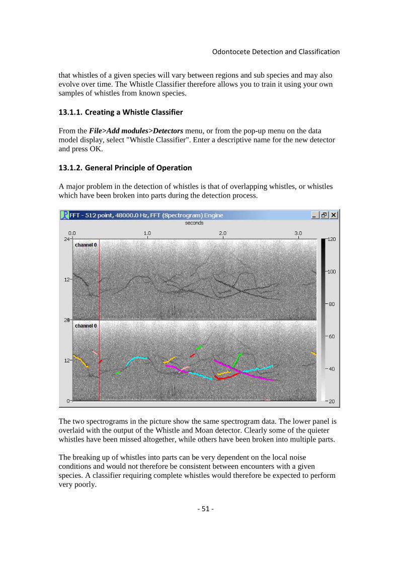
Odontocete Detection and Classification
- 51 -
that whistles of a given species will vary between regions and sub species and may also evolve over time. The Whistle Classifier therefore allows you to train it using your own samples of whistles from known species.
13.1.1. Creating a Whistle Classifier
From the File>Add modules>Detectors menu, or from the pop-up menu on the data model display, select "Whistle Classifier". Enter a descriptive name for the new detector and press OK.
13.1.2. General Principle of Operation
A major problem in the detection of whistles is that of overlapping whistles, or whistles which have been broken into parts during the detection process.
The two spectrograms in the picture show the same spectrogram data. The lower panel is overlaid with the output of the Whistle and Moan detector. Clearly some of the quieter whistles have been missed altogether, while others have been broken into multiple parts.
The breaking up of whistles into parts can be very dependent on the local noise conditions and would not therefore be consistent between encounters with a given species. A classifier requiring complete whistles would therefore be expected to perform very poorly.

Odontocete Detection and Classification
- 52 -
The PAMGUARD Whistle Classifier therefore works by taking short fragments of whistles and accumulates statistics over many fragments. Since the level of "natural" fragmentation due to noise will vary, all detected whistles are first broken into fragments of the same length prior to classification. While fragmenting whistles in this way is discarding potentially useful information, it creates an overall improvement in classifier stability
For each whistle fragment, three parameters are measured:
• The start frequency
• The slope
• The curvature
Distributions of these three parameters are built up over time, then once sufficient fragments have been accumulated, the mean, the standard deviation and the skew (lopsidedness) of each distribution is measured, giving a total of nine parameters which are used by the statistical classifier, i.e.
• The mean start frequency
• The standard deviation of the distribution of start frequencies
• The skew of the mean frequency distribution
• The mean slope
• etc. ...
Next: Configuring the Whistle Classifier
13.2. Configuration
The Detection / Whistle Classifier menu has two sub menus: Settings... and Discriminant
Function Training...
13.2.1. Settings Menu
From the settings menu a dialog will appear, the top half of which will contain a drop down list of data sources and buttons to select the operation mode.
Odontocete Detection and Classification
- 53 -
Data Source
Select the data source. This should be the connected regions output from a Whistle and Tone
detector.
Operation Mode
Select either Run Classifier, in which case new detections from the Whistle and Tone
detector will be fragmented and the fragments sent for classification, or Collect Training Data in which case the contours of detected whistles will be stored for Discriminant Function Training
Previous: Whistle Classifier Overview
Next: Collecting Training Data
13.3. Collecting Training Data
From the Whistle Classifier Settings dialog, select "Collect Training Data" and the dialog will change to show training data parameters in it's lower half.
The linked image cannot be displayed. The file may have been moved, renamed, or deleted. Verify that the link points to the correct file and location.

Odontocete Detection and Classification
- 54 -
During the collection of training data, whistles will be extracted from raw audio data and stored in a file, or set of files on your hard drive ready for Discriminant Function Training at a later date
13.3.1. Data Organisation
Although in principle, the classifier can collect training data in real time (i.e. directly from a sound card connected to a hydrophone in the water, it is far more likely that you will be training your classifier based on a set of previously recorded sound files which you have archived over a period of time.
Sound files should ideally all be recorded at the same sample rate and have the same number of channels. If possible, organise your sound files so that you have one file folder per species and all the species folders are sub folders of a master training data folder as shown below.
The linked image cannot be displayed. The file may have been moved, renamed, or deleted. Verify that the link points to the correct file and location.
Odontocete Detection and Classification
- 55 -
Organising your data in this way is not essential, but it does mean that processing of all files can take place as a single operation (e.g. over the weekend)
Sound Acquisition
Set up your Sound Acquisition module to analyse data from file folders, set the file folder to be the root directory containing your folders of files by species and check the option to include sub folders. Do not check the option to merge contiguous files so that processing stops and starts at the end of each file.
The linked image cannot be displayed. The file may have been moved, renamed, or deleted. Verify that the link points to the correct file and location.

Odontocete Detection and Classification
- 56 -
Species Names
If your data have been organised into folders as described above, the classifier can use the folder names as species names.
If your data are not organised in the way described above, then you will need to enter the species name for the training set you are working on (which should of course now be just of a single species).
Storage Folder
Training data are stored in files with the ending .wctd (Whistle Classifier Training Data). One wctd file will be created for each sound file analysed. Use the Browse button to select the folder you want these files to be stored in.
Running
Run PAMGUARD. All the files in the directory structure of training data will be processed and .wctd files created in your output folder. The main classifier display will show distributions of whistle fragment parameter but will not be performing classification.
There are of course other ways of organising your training data. For instance, if you wish to add new data to an already existing training set, it is not necessary to reprocess all the data.
The linked image cannot be displayed. The file may have been moved, renamed, or deleted. Verify that the link points to the correct file and location.

Odontocete Detection and Classification
- 57 -
Once you have created your .wctd files, you will need to run the Discriminant Function
Training before you can use the classifier on new data
Previous: Configuring the Whistle Classifier
Next: Discriminant Function Training
13.4. Discriminant Function Training
Discriminant Function Training is controlled from the Detection / Whistle Classifier / Discriminant Function Training ... menu.
13.4.1. Training Data
Before running the training algorithms, you must process raw audio files for each species to create a training data set as described in the Collecting Training Data section. Training data will be in the form of a number of .wctd files containing extracted whistle contours from the Whistle and Moan detector
Select the file folder containing your .wctd files. The files can all be in the same folder or can be split into sub folders, in which case you should check the "Select Sub folders" option.
The linked image cannot be displayed. The file may have been moved, renamed, or deleted. Verify that the link points to the correct file and location.
Odontocete Detection and Classification
- 58 -
species names
When the wctd files were created, the species name (either input by the user of taken from the folder name of the source audio file) was written into each file. Species names from the .wctd files are used by default during the classifier training. However, it is possible to override the species names in the .wctd files by organising you .wctd files into sub folders with different names and selecting the "Use folder names as species names" option.
This allows you to merge data sets which may have been given slightly different names by different analyst (for instance, different people may have labelled training data for Bottlnose dolphin as "BND", "Bottlenose", "TT", "Tursiops", etc. It also allows you to merge species into groups, for instance, you might have a new "Small dolphin" category containing data for both common and striped dolphin.
13.4.2. Run Training
To run the training, set the following parameters:
Classifier Type - Two discriminant functions are available, Linear Discriminant Analysis and a Mahalanobis Distances Classifier.
Fragment Length - How long the fragments of whistle fed into the classifier should be.
Section length - how many fragments to accumulate before extracting parameters from the distribution and running a classification.
Number of test bootstraps = The number of randomised trials to run when testing classifier performance
Frequency range for search - The frequency range to use. Contours outside this range will be discarded.
Press the "Start Training" button and wait while the classifier training process runs.
Progress will be indicated in the bar at the bottom of the window and also as text output in the right hand display panel.
13.4.3. Training Output
The training process produces a number of matrices which will control the classification process. These are automatically stored into the standard PAMGUARD settings file you are currently using.

Odontocete Detection and Classification
- 59 -
You can also export the classifier settings to a Whistle Classifier Settings (*.wcsd) file for archiving and easy sharing with other users so that they can set up the same classifier without requiring access to the training data set.
Previous: Collecting Training Data
Next: Running the Whistle Classifier
13.5. Running the Whistle Classifier
From the Whistle Classification settings dialog, select "Run classifier" as the operation mode and the dialog will look something like the one below.
13.5.1. When to Classify
The classifier will take whistles from the data source, break them into fragments and accumulate fragments until there are the same number of fragments as were used during

Odontocete Detection and Classification
- 60 -
training. It will then classify the data based on the distributions of extracted parameters, output the classification result, clear the distributions and start over
Sometimes, even if there are no real whistles, a few false detections are occurring from noise. These will gradually accumulate and cause false classifications. You can set the Classifier to clear the distributions if the whistle rate drops too low using the parameters in the "When to Classify" section of the dialog.
13.5.2. Classifier Training Parameters
There are two ways of setting the classifier training parameters:
Either they will have been set when you ran the Discriminant Function Training
Or you can load a set of training parameters from a Whistle Classifier Settings (*.wcsd) file provided to you by someone else.
To load parameters from a .wcsd file, press the 'Select ...' button and navigate to the file on your hard drive. the parameters will be loaded into your PAMGUARD configuration, so you will only need to access the file once.
The remainder of the dialog shows information about how the training was set up (fragment length, frequency range, etc.). Since these parameters must be identical when you run the classifier to parameters used when training the classifier, you are unable to change any of these parameters.
Previous: Discriminant Function Training
Next: Whistle Classifier Output
13.6. Whistle Classifier Output
13.6.1. Graphical Output
Classifier output is shown graphically on a tab on the main PAMGUARD display.

Odontocete Detection and Classification
- 61 -
Parameter Distributions
The top half of the display shows the distributions of parameters extracted from each whistle fragment (Note that the negative and positive inflections are not currently used).
Classifier History
The bottom half of the display shows the classification history.
Each time the parameter distributions build up enough data and the classification runs, the classification probability for each possible species with a probability > 1% (0.01) is displayed
The time axis of the display is logarithmic, so recent history (i.e. what's happened in the last minute) gets as much space as the preceding 10 minutes or the 100 minutes before that. A total of two hours of data are shown.
The linked image cannot be displayed. The file may have been moved, renamed, or deleted. Verify that the link points to the correct file and location.

Odontocete Detection and Classification
- 62 -
Database Output
If a Database is being used, each classification result is also written to the database.
Previous: Running the Whistle Classifier

Odontocete Detection and Classification
- 63 -
Appendix 3: Click Classification Help Pages
Appendix 4: Click Detector
4.1 Click Classification
4.1.1 Overview
Individual clicks detected by the click detector can be classified using one of two different click classifiers. The first, Basic click Classifier is the same as the click classifier in the IFAW RainbowClick software. the basic classifier is generally adequate for the classification of high frequency harbour porpoise clicks and is primarily retained for backwards compatibility with the RainbowClick classifier. The second Classifier With
Frequency Sweep uses additional classification parameters and is more suitable for the detection of lower frequency odontocete clicks, particularly those of beaked whales.
The classifier is set up from the
Click Detection>Click Classification menu.
4.1.2 Click Classifier Selection
Select the type of click classifier you wish to use from the drop down list. This will either be the Basic click Classifier or the Classifier With Frequency Sweep.
The linked image cannot be displayed. The file may have been moved, renamed, or deleted. Verify that the link points to the correct file and location.

Odontocete Detection and Classification
- 64 -
You must also check the "Run classification online" box if you want clicks to be processed as they are detected.
You should check the "Discard unclassified clicks" box if you want clicks which do not pass any of the classification criteria to be discarded. Use this feature with great caution and only when you are confident that the classifiers are working well for the clicks that you do want.
4.1.3 Click Types
The click classification dialog contains a list of defined click types.
If more than one type is defined, then each click is tested against each type in sequence and the click is classified as belonging to the first type with a matching set of classification criteria.
If the click does not match the criteria of any of the classifiers, then it is unclassified.
Use the New, Edit and Delete buttons to add, modify and remove items from the list.
Each click is checked against the different click types in sequence. As soon as one set of criteria is matched, the classifier will stop searching other click types. It is therefore sometimes important to arrange the different types in a particular order. Use the Up and Down buttons to move different click types up and down in the list.
Individual species classifiers can be enabled or disabled, for example if you wish to temporarily stop checking for a particular click type
Classified clicks can also be discarded. For example, if there was a particular noise source causing false triggers of the click detector (e.g. a depth sounder), it may be possible to set up a classifier for those detections and immediately discard them.
If either the New or the Edit button is pressed, the Individual Click Classification dialog will be displayed. The behaviour of this dialog will depend on the type of classifier selected.
Previous:Click Detector
Next: Basic Click Classification
13.7. Click Classification With Frequency Sweep
Odontocete Detection and Classification
- 65 -
13.7.1. Overview
The click classifier with frequency sweep was added to PAMGUARD in 2010 to provide a wider choice of species identification parameters, particularly for the detection of beaked whales.
Operation is similar to that of the Basic click Classifier in so much that a number of different tests can be carried out on each click and the click will have to satisfy all of those tests in order to be classified.
13.7.2. General options
In the general options section, enter the species name, a unique identification code and select the symbol to be used for this species on the click detector display.
Channel options
Click detection is generally conducted on more than one channel. If this is the case, then the click classifier can be set to either:
The linked image cannot be displayed. The file may have been moved, renamed, or deleted. Verify that the link points to the correct file and location.

Odontocete Detection and Classification
- 66 -
1. Require positive identification on all channels individually
2. Require positive identification on only one channel
3. Use mean parameter values over all channels
Restricting the click length
Click waveforms from the click detector are generally longer than the click itself. This is partly due to the pre and post samples added to the waveform but can also be caused by the click arriving at different times on different channels. The addition of extra waveform data before or after the click has little effect if the click has a high signal to noise ratio, but for quiet clicks, the additional data is a significant source of noise for some parameter measurements. There is therefore an option to restrict the length of the data used in the parameter extractions. If this option is used, then the peak of the waveform envelope is found (see Click Length below) and an equal amount of wave data taken from each side of the envelope maximum.
Generally the click length should be set to a power of 2 (e.g. 128, 256, 512, etc) since the FFT's used in many of the calculations require data that is an exact power of 2 long. Other values can be used, in which case the shortened data will be padded with zeros prior to FFT calculations.
13.7.3. Click Length
The click length is measured by first calculating the analytic waveform (or signal envelope) of the click using the Hilbert transform of the waveform data
This is then smoothed using a moving average filter defined by the user (smoothing parameter in dialog).
The maximum of the smoothed envelope is then found and the click length taken as the length of the data between points either side of that maximum which remain above the maximum value minus the threshold (Threshold parameter in dialog).
The test is passed if the click length lies within the range set by the user (Length range parameters in dialog).
13.7.4. Energy Bands
The energy band test compares the acoustic energy in a test band with the energy in two control bands.
The user should enter the frequency ranges of each band and a threshold value for each of the control bands. The test is passed if the test band energy exceeds each of the control band energies by more than the threshold values.

Odontocete Detection and Classification
- 67 -
If only one control band is required, set both frequency limits of the second control band to zero.
13.7.5. Peak and Mean Frequency
The peak and mean frequency are measured from the power spectrum of the click waveform.
Search and integration range
The peak search and the frequencies over which the mean frequency is summed can be restricted using the search and integration range parameters in the dialog.
The power spectrum can also be smoothed using a moving average filter to remove noisy spikes from the spectral data.
Peak Frequency
If the peak frequency test is enabled, the peak frequency (taken as the highest point in the smoothed spectral data between the limits of the Search and Integration range) must lie between the limits entered in the dialog.
Peak Width
The width of the spectral peak is measured by first finding the amplitude of the power spectrum at the peak frequency. The peak width is taken as the frequency range of the data either side of that peak which are at an amplitude above the peak amplitude minus the threshold (threshold parameter in dialog). The test is passed if the width of the peak lies within the set range.
Mean Frequency
The mean frequency is calculated using
where
i is the range of frequency bins within the search and integration range
I is the intensity of the spectrum at each frequency bin i
f is the frequency (Hz) at each frequency bin i
The linked image cannot be displayed. The file may have been moved, renamed, or deleted. Verify that the link points to the correct file and location.

Odontocete Detection and Classification
- 68 -
The test is passed if the mean frequency lies within the set range.
13.7.6. Zero Crossings
Some species of whale produce frequency modulated clicks, i.e. the click frequency changes during the course of the click.
The power spectrum of a click is an average of the spectral energy over the duration of the click and is therefore unable to show changes in frequency during the course of the click.
Although it is possible to extract more detailed frequency information using a Wigner-Ville
transform of the waveform data. These are slow to compute and therefore not suitable for real time classification.
The classifier therefore extracts frequency information by examining zero crossings of the waveform data.
A zero crossing is defined as the signal waveform going from a positive to a negative value or vice-versa. The classifier searches the waveform for zero crossings only within the region of the click between the thresholded limits from the click length estimation described above.
Once zero crossings have been found, the frequency between each zero crossing is calculated. If there are three or more zero crossings (permitting two or more estimates of frequency) the frequency sweep is calculated by fitting a linear model of frequency against time.
Two tests can then be applied to the data. The first is the total number of zero crossings which must lie within the range set in the dialog. The second is the frequency sweep estimated from the zero crossing data.
13.7.7. Species Default settings
The 'Species Defaults' button allows the user to use stored standard settings for beaked whale and harbour porpoise classifiers.
Previous: Basic Click Classification
Next: Click Train Identification