Development and Applications of Advanced Electronic...
205
Development and Applications of Advanced Electronic Structure Methods By Franziska Bell A dissertation submitted in partial satisfaction of the requirements for the degree of Doctor in Philosophy in Chemistry in the Graduate Division of the University of California, Berkeley Committee in charge: Professor Martin Head-Gordon, Chair Professor William H. Miller Professor Alexis T. Bell Spring 2012
Transcript of Development and Applications of Advanced Electronic...

Development and Applications of Advanced Electronic
Structure Methods
By
Franziska Bell
A dissertation submitted in partial satisfaction of the
requirements for the degree of
Doctor in Philosophy
in
Chemistry
in the
Graduate Division
of the
University of California, Berkeley
Committee in charge:
Professor Martin Head-Gordon, ChairProfessor William H. Miller
Professor Alexis T. Bell
Spring 2012
Development and Applications of Advanced Electronic Structure Methods
Copyright 2012
by
Franziska Bell
Abstract
Development and Applications of Advanced Electronic
Structure Methods
by
Franziska Bell
Doctor of Philosophy in Chemistry
University of California, Berkeley
Professor Martin Head-Gordon, Chair
This dissertation contributes to three different areas in electronic struc-ture theory. The first part of this thesis advances the fundamentals of orbitalactive spaces. Orbital active spaces are not only essential in multi-referenceapproaches, but have also become of interest in single-reference methods asthey allow otherwise intractably large systems to be studied. However, de-spite their great importance, the optimal choice and, more importantly, theirphysical significance are still not fully understood. In order to address thisproblem, we studied the higher-order singular value decomposition (HOSVD)in the context of electronic structure methods. We were able to gain a phys-ical understanding of the resulting orbitals and proved a connection to un-relaxed natural orbitals in the case of Møller-Plesset perturbation theory tosecond order (MP2). In the quest to find the optimal choice of the activespace, we proposed a HOSVD for energy-weighted integrals, which yieldedthe fastest convergence in MP2 correlation energy for small- to medium-sizedactive spaces to date, and is also potentially transferable to coupled-clustertheory.
In the second part, we studied monomeric and dimeric glycerol radi-cal cations and their photo-induced dissociation in collaboration with Prof.Leone and his group. Understanding the mechanistic details involved in theseprocesses are essential for further studies on the combustion of glycerol and
1

carbohydrates. To our surprise, we found that in most cases, the experi-mentally observed appearance energies arise from the separation of productfragments from one another rather than rearrangement to products.
The final chapters of this work focus on the development, assessment, andapplication of the spin-flip method, which is a single-reference approach, butcapable of describing multi-reference problems. Systems exhibiting multi-reference character, which arises from the (near-) degeneracy of orbital en-ergies, are amongst the most interesting in chemistry, biology and materialsscience, yet amongst the most challenging to study with electronic structuremethods. In particular, we explored a substituted dimeric BPBP moleculewith potential tetraradical character, which gained attention as one of themost promising candidates for an organic conductor. Furthermore, we ex-tended the spin-flip approach to include variable orbital active spaces andmultiple spin-flips. This allowed us to perform wave-function-based studiesof ground- and excited-states of polynuclear metal complexes, polyradicals,and bond-dissociation processes involving three or more bonds.
2

.
To allwho walked this path with me,
but most of all,my beloved mother.
i

ii

Contents
1 Introduction 11.1 Elementary Electronic Structure Theory . . . . . . . . . . . . 11.2 Wavefunction based Methods . . . . . . . . . . . . . . . . . . 3
1.2.1 Hartree-Fock Theory . . . . . . . . . . . . . . . . . . . 31.2.2 Weak Correlation . . . . . . . . . . . . . . . . . . . . . 5
1.2.2.1 Møller Plesset Perturbation Theory . . . . . . 51.2.2.2 MP2 Theory . . . . . . . . . . . . . . . . . . 61.2.2.3 Configuration Interaction Theory . . . . . . . 71.2.2.4 Coupled-Cluster Theory . . . . . . . . . . . . 8
1.2.3 Strong Correlation Methods . . . . . . . . . . . . . . . 91.2.3.1 MCSCF, CASSCF and RASSCF . . . . . . . 9
1.2.4 Single Reference-based Approaches for Strong Corre-lation Problems . . . . . . . . . . . . . . . . . . . . . . 11
1.3 Reduction of the Parameter Space . . . . . . . . . . . . . . . . 131.4 Density Functional Theory . . . . . . . . . . . . . . . . . . . . 15
2 HOSVD in Quantum Chemistry 172.1 Introduction . . . . . . . . . . . . . . . . . . . . . . . . . . . . 18
2.1.1 Motivation . . . . . . . . . . . . . . . . . . . . . . . . . 182.1.2 Notation and Basic Definitions . . . . . . . . . . . . . 182.1.3 Overview of Tensor Decompositions and Their Rela-
tion to Quantum Chemistry . . . . . . . . . . . . . . . 192.2 Theory . . . . . . . . . . . . . . . . . . . . . . . . . . . . . . . 22
2.2.1 Review of HOSVD without any numerical approxima-tions such as rank truncation (untruncated HOSVD) . 22
2.2.2 rank-(R1, R2, ..., Rd) truncated HOSVD . . . . . . . . . 232.2.3 Computational cost of HOSVD . . . . . . . . . . . . . 24
2.3 Results . . . . . . . . . . . . . . . . . . . . . . . . . . . . . . . 24
iii

2.3.1 Numerical Results . . . . . . . . . . . . . . . . . . . . 242.3.2 Connection between HOSVD T2 and MP2 Natural Or-
bitals . . . . . . . . . . . . . . . . . . . . . . . . . . . . 352.3.3 Higher Order Orthogonal Iterations (HOOI) vs. HOSVD 40
2.4 Conclusion . . . . . . . . . . . . . . . . . . . . . . . . . . . . . 40
3 HOSVD of Energy-Weighted Integrals 453.1 Introduction . . . . . . . . . . . . . . . . . . . . . . . . . . . . 453.2 Notation and Basic Definitions . . . . . . . . . . . . . . . . . . 473.3 Theory . . . . . . . . . . . . . . . . . . . . . . . . . . . . . . . 47
3.3.1 Overview of the HOSVD . . . . . . . . . . . . . . . . . 473.3.2 HOOI vs. Orbital Optimization for MP2 . . . . . . . . 493.3.3 Proposed Coordinate Transformation for MP2 . . . . . 52
3.4 Numerical Results . . . . . . . . . . . . . . . . . . . . . . . . . 573.5 Transferability to Coupled-Cluster Methods . . . . . . . . . . 603.6 Conclusions . . . . . . . . . . . . . . . . . . . . . . . . . . . . 64
4 Glycerol Photodissociation 654.1 Introduction . . . . . . . . . . . . . . . . . . . . . . . . . . . . 654.2 Methods . . . . . . . . . . . . . . . . . . . . . . . . . . . . . . 67
4.2.1 Experimental . . . . . . . . . . . . . . . . . . . . . . . 674.2.2 Computational . . . . . . . . . . . . . . . . . . . . . . 68
4.2.2.1 Neutral and Radical Conformers . . . . . . . 684.2.2.2 Ionization Potentials . . . . . . . . . . . . . . 694.2.2.3 Transition States . . . . . . . . . . . . . . . . 694.2.2.4 Choice of Functional . . . . . . . . . . . . . . 704.2.2.5 Dimeric Glycerol . . . . . . . . . . . . . . . . 70
4.3 Results and Discussion . . . . . . . . . . . . . . . . . . . . . . 704.3.1 Experimental Measurements . . . . . . . . . . . . . . . 704.3.2 Monomeric Glycerol . . . . . . . . . . . . . . . . . . . 75
4.3.2.1 Neutral Conformers . . . . . . . . . . . . . . 754.3.2.2 Radical Cation Conformers . . . . . . . . . . 764.3.2.3 Water Loss (74 m/z) . . . . . . . . . . . . . . 834.3.2.4 62 m/z . . . . . . . . . . . . . . . . . . . . . 874.3.2.5 61 m/z . . . . . . . . . . . . . . . . . . . . . 894.3.2.6 60 m/z . . . . . . . . . . . . . . . . . . . . . 904.3.2.7 45 m/z . . . . . . . . . . . . . . . . . . . . . 914.3.2.8 44 m/z . . . . . . . . . . . . . . . . . . . . . 92
iv

4.3.2.9 43 m/z . . . . . . . . . . . . . . . . . . . . . 934.3.2.10 Formation of CHxO
+ and smaller fragment ions 944.3.2.11 Comparison to Neutral/Protonated Glycerol . 94
4.3.3 Dimeric Glycerol . . . . . . . . . . . . . . . . . . . . . 954.3.3.1 153 m/z . . . . . . . . . . . . . . . . . . . . . 974.3.3.2 136 m/z . . . . . . . . . . . . . . . . . . . . . 974.3.3.3 93 m/z and 185 m/z . . . . . . . . . . . . . . 98
4.4 Conclusions . . . . . . . . . . . . . . . . . . . . . . . . . . . . 98
5 Substituted PBPB Dimers 1015.1 Introduction . . . . . . . . . . . . . . . . . . . . . . . . . . . . 1025.2 Computational Details . . . . . . . . . . . . . . . . . . . . . . 1045.3 Results and Discussion . . . . . . . . . . . . . . . . . . . . . . 105
5.3.1 Molecular Geometries . . . . . . . . . . . . . . . . . . . 1055.3.2 Relative Stability . . . . . . . . . . . . . . . . . . . . . 1105.3.3 Communication between Diradical Sites . . . . . . . . 1115.3.4 Radical Character . . . . . . . . . . . . . . . . . . . . . 1135.3.5 Low-lying Excited States and Magnetic Couplings . . . 1175.3.6 Magnetic Couplings . . . . . . . . . . . . . . . . . . . . 118
5.4 Conclusions . . . . . . . . . . . . . . . . . . . . . . . . . . . . 120
6 Restricted Active Space Spin-Flip (RAS-SF) with ArbitraryNumber of Spin-Flips 1276.1 Introduction . . . . . . . . . . . . . . . . . . . . . . . . . . . . 1276.2 Theory . . . . . . . . . . . . . . . . . . . . . . . . . . . . . . . 130
6.2.1 FCI in the active space, A (RAS-II) . . . . . . . . . . . 1316.2.2 Properties of RAS-SF . . . . . . . . . . . . . . . . . . . 132
6.3 Computational Details . . . . . . . . . . . . . . . . . . . . . . 1326.4 Results and Discussion . . . . . . . . . . . . . . . . . . . . . . 133
6.4.1 Bond Dissociation . . . . . . . . . . . . . . . . . . . . . 1336.4.2 Binuclear Metal Complexes . . . . . . . . . . . . . . . 134
6.4.2.1 µ-hydroxo-bis[pentaaminechromium(III)] Cation1356.4.2.2 µ-oxo-bis[pentaamminechromium-(III)] . . . . 1356.4.2.3 trans-[HO-Cr(cyclam)-NC-Cr(CN)5]− . . . . . 1376.4.2.4 Co2O4 . . . . . . . . . . . . . . . . . . . . . . 1386.4.2.5 [(TPA*)Co(II)(DHBQ2−)Co(II)(TPA*)]2+ . . 139
6.4.3 Organic Polyradicals . . . . . . . . . . . . . . . . . . . 1406.4.3.1 Linear Carbenes . . . . . . . . . . . . . . . . 141
v
6.4.3.2 Branched Carbenes . . . . . . . . . . . . . . . 1436.4.3.2.1 Polycarbene m = 3 . . . . . . . . . . . . . . . . . . . . 1436.4.3.2.2 Catenated Closs Radicals . . . . . . . . . . . . . . . . 144
6.5 Conclusions . . . . . . . . . . . . . . . . . . . . . . . . . . . . 146
7 Appendix: Glycerol Photodissociation 179
vi

List of Figures
2.1 HOSVD procedure. Adapted from [1]. . . . . . . . . . . . . . 232.2 Comparison of the original T2 amplitudes and those decom-
posed using the HOSVD (H2/6-31G(3df,3pd)). . . . . . . . . 252.3 Percent MP2 correlation energy vs. number of amplitudes
included (H2/6-31G**) . . . . . . . . . . . . . . . . . . . . . . 262.4 Percent MP2 correlation energy vs. number of amplitudes
included (H2/6-31++G**) . . . . . . . . . . . . . . . . . . . . 272.5 recovery of % MP2 correlation energy vs. number of virtual
orbitals included for H2 at equilibrium bond distance in variousbasis sets. Box: the four most correlating virtual orbitals. . . . 32
2.6 recovery of % MP2 correlation energy vs. number of virtualorbitals included for linear H4 (R1 = 0.76A, R2 = 1.2 A) invarious basis sets. Box: the eight most correlating virtualorbitals. . . . . . . . . . . . . . . . . . . . . . . . . . . . . . . 35
2.7 recovery of % MP2 correlation energy vs. active space (oc-cupied, virtual) included for linear N2 at equilibrium bonddistance in various basis sets. Boxes: the five most correlat-ing virtual orbitals for HOSVD and HF. (HOSVD order inbrackets) (cutoff: 0.3) . . . . . . . . . . . . . . . . . . . . . . 36
2.8 recovery of % MP2 correlation energy vs. number of virtualorbitals included for N2 at equilibrium bond distance in variousbasis sets. . . . . . . . . . . . . . . . . . . . . . . . . . . . . . 37
2.9 HF and HOSVD orbitals for H2/6-31G**, as well as MO dif-ferences (cutoff: 0.15) . . . . . . . . . . . . . . . . . . . . . . . 38
2.10 HF and HOSVD orbitals for H4/6-31G** (R1 = 0.76 A, R2 =1.2A), as well as MO differences (cutoff: 0.15) . . . . . . . . . 39
2.11 HF and HOSVD occupied orbitals for N2/6-31G* (at equilib-rium), as well as MO differences (cutoff: 0.15) . . . . . . . . . 42
vii

2.12 HF and HOSVD virtual orbitals for N2/6-31G* (at equilib-rium), as well as differences in their coefficients (cutoff: 0.15) . 43
2.13 HOSVD occupied-virtual correlating orbital pairs for CH4 (cut-off: 0.2) (6-31G**; MP2 optimized geometry) . . . . . . . . . 44
2.14 Adapted from [1]. Alternating least squares algorithm to com-pute a rank-(R1, R2, ..., Rd) Tucker decomposition for a tensor,T ∈ RI1×I2×...×Id . Also known as the higher-order orthogonaliteration (HOOI). . . . . . . . . . . . . . . . . . . . . . . . . . 44
3.1 Comparison of HOOI of MP2 amplitudes and norm-preservingorbital-optimized MP2 (H2O, cc-pVDZ) . . . . . . . . . . . . . 50
3.2 Extension to Figure 3.1: Energetic differences (a.u.) in theHOOI of MP2 amplitudes and norm-preserving orbital-optimizedMP2 (H2O, cc-pVDZ) . . . . . . . . . . . . . . . . . . . . . . 51
3.3 HOOI procedure. Adapted from [2]. . . . . . . . . . . . . . . 53
3.4 Recovery of percent MP2 correlation energy vs. number ofvirtual orbitals included for CH4 at its equilibrium geometry(cc-pVDZ) . . . . . . . . . . . . . . . . . . . . . . . . . . . . . 59
3.5 Recovery of percent MP2 correlation energy vs. number ofvirtual orbitals included for H2O at its equilibrium geometry(cc-pVDZ) . . . . . . . . . . . . . . . . . . . . . . . . . . . . . 60
3.6 Recovery of percent MP2 correlation energy vs. number ofvirtual orbitals included for H2O at its equilibrium geometry(cc-pVTZ). For clarity only the first 20 of 53 virtual orbitalsare shown. . . . . . . . . . . . . . . . . . . . . . . . . . . . . . 61
3.7 Recovery of percent MP2 correlation energy vs. number ofvirtual orbitals included for CO at its equilibrium geometry(cc-pVDZ). . . . . . . . . . . . . . . . . . . . . . . . . . . . . 62
4.1 Photoionization TOF mass spectrum of glycerol in (a) super-sonic expansion, (b) effusive source and (c) D5-glycerol in aeffusive source at 10.5 eV . . . . . . . . . . . . . . . . . . . . . 72
4.2 (a) Normalized PIE curves for the parent ion C3H8O+3 . The
adiabatic IE is found to be 9.4±0.1 eV (supersonic expan-sion). (b)-(d) Normalized PIE curves for C3H6O+
2 , C2H6O+2
and C2H4O+, respectively. Red circles: supersonic expansion,black triangles: effusive conditions. AEs shown are from thesupersonic expansion. . . . . . . . . . . . . . . . . . . . . . . 73
viii

4.3 The energetically two lowest neutral gas-phase conformers.Left: conformer 95, right: conformer 100 . . . . . . . . . . . . 76
4.4 Representative conformers from each of the main sub-classesfor gas-phase monomeric radical glycerol. . . . . . . . . . . . . 80
4.5 Proposed mechanisms for water loss (74 m/z), concerted reac-tion involving a 6-membered proton-transfer . . . . . . . . . . 85
4.6 Other mechanisms considered for water loss (74 m/z), 5-memberedtransition state . . . . . . . . . . . . . . . . . . . . . . . . . . 86
4.7 Other mechanisms considered for water loss (74 m/z), directepoxide formation, ether intermediate, and C-H abstraction . . 86
4.8 Other mechanisms considered for water loss (74 m/z), via C-2bound H2O intermediate . . . . . . . . . . . . . . . . . . . . . 87
4.9 Energetic overview of the excluded water loss channels (ωB97X/6-31+G∗∗) . . . . . . . . . . . . . . . . . . . . . . . . . . . . . . 88
4.10 intermediate 1, INT1 . . . . . . . . . . . . . . . . . . . . . . . 89
4.11 Proposed mechanisms for formation of fragment 62 m/z. . . . 89
4.12 IRC following reactant (radical conformer 100) to the productcomplex. Full separation to products also does not feature anexit barrier. . . . . . . . . . . . . . . . . . . . . . . . . . . . . 90
4.13 Proposed mechanism for formation of fragment 61 m/z. . . . . 91
4.14 Proposed mechanisms for formation of fragment 60 m/z. . . . 91
4.15 Proposed mechanism for formation of fragment 45 m/z. . . . . 92
4.16 Proposed mechanisms for water loss (74 m/z), formaldehydeloss (62 m/z) and formation of 44 m/z (vinyl alcohol) . . . . . 93
4.17 Proposed mechanism for formation of fragment 43 m/z. . . . . 94
4.18 Cartoon of the lowest energy dimer structure (conformer 1),highlighting the hydrogen bonding network . . . . . . . . . . . 96
4.19 Spin density in dimeric glycerol radical cation (cutoff: 0.02) . 97
5.1 Overview of the most important structures. Para and metaconformations are specified by p- and m- prefixes. A and B la-belling indicates planar (1,3-diborata-2,4-diphosphoniocyclobutane-1,3-diyl) and bicycle (1,3-diborata-2,4-diphosphoniobicyclo[1.1.0]butane)rearrangements of the PBPB moieties, respectively. Num-bers 1, 2 and 3 correspond to PBPB monomer, phenyl-PBPBmolecule and PBPB dimer, respectively. . . . . . . . . . . . . 103
ix

5.2 Atomic labeling of PBPB used in the description of geomet-rical parameters (Tables 7.1-5.3). Although the B-B bond isnot represented, labels are applicable for both, planar (A) andbicyclic (B) molecules. . . . . . . . . . . . . . . . . . . . . . . 106
5.3 Delocalization energy in para isomers. Delocalization energyis defined as the difference between the energy cost of twistingthe phenyl ring (a) and two times the twisting energy withoutone of the PBPB units (b). The same scheme is applied forfully (p-1A, R = iPr, R = tBu) and H-substituted (p-1AH,R, R = H) molecules. . . . . . . . . . . . . . . . . . . . . . . . 112
5.4 B3LYP/6-31G(d) optimized geometry of m-3A with some shortH· · ·H distances indicated (in A). . . . . . . . . . . . . . . . . 113
5.5 Diagrammatic representation of the quadruple cluster excita-tion from the HOMO-1 and HOMO to the LUMO and LUMO+1orbitals. . . . . . . . . . . . . . . . . . . . . . . . . . . . . . . 116
5.6 State energy diagram (in kcal/mol) computed at RAS-2SF/6-31G(d) computational level for p-3A, p-3AH, m-3A and m-3AH. All energies are given with the respective ground stateas reference. . . . . . . . . . . . . . . . . . . . . . . . . . . . . 122
5.7 RAS-2SF natural orbitals of p-3AH and m-3AH. RAS-2SFand CASSCF(4,4) (in italics) orbital occupations are also in-dicated. . . . . . . . . . . . . . . . . . . . . . . . . . . . . . . 123
5.8 Four paramagnetic center model for the para and meta sys-tems. First neighbors exchange constants (σ and λ) are indi-cated by arrows between centers. . . . . . . . . . . . . . . . . 124
5.9 Short (σ) and long (λ) range energy splitting in the four para-magnetic centers models of Figure 5.3.6. A and B indicatesymmetrical and asymmetrical rotation around the principalaxis, respectively. . . . . . . . . . . . . . . . . . . . . . . . . . 125
6.1 Orbital subspaces in the RAS-SF approach. Adapted from [3]. 1316.2 Dissociation curve for the N2 molecule (cc-pVTZ) . . . . . . . 1336.3 Binuclear Cr(III)-Cr(III) complex, [Cr2(NH3)10(OH)]5+. Hy-
drogen atoms omitted for clarity. . . . . . . . . . . . . . . . . 1366.4 Binuclear Cr(III)-Cr(III) complex, [Cr2(NH3)10(O)]4+ . . . . . 1376.5 trans-[HO-Cr(cyclam)-NC-Cr(CN)5]− . . . . . . . . . . . . . . 1386.6 Co2O4. Structure from [4]. . . . . . . . . . . . . . . . . . . . . 1396.7 Binuclear Co2(II) complex, [(TPA*)Co(II)(DHBQ2−)CO(II)(TPA*)]2+140
x

6.8 One- and two-dimensional carbenes. (n = 1− 5, m = 3, 6, 9) . 1436.9 Catenated Closs Radicals: Structure 1 . . . . . . . . . . . . . 1496.10 Model systems used in [5] to study relative stabilities of cate-
nated Closs radicals. . . . . . . . . . . . . . . . . . . . . . . . 149
xi

xii
List of Tables
2.1 Computational cost of HOSVD . . . . . . . . . . . . . . . . . 24
2.2 HOSVD vs. Original compression factors γOrig/HOSVD for agiven % correlation energy - Pople style bases; Hn: R1 = 0.76,R2 = 1.2 . . . . . . . . . . . . . . . . . . . . . . . . . . . . . 28
2.3 HOSVD vs. Original compression factors γOrig/HOSVD for agiven % correlation energy - Dunning style bases; Hn: R1 =0.76, R2 = 1.2 . . . . . . . . . . . . . . . . . . . . . . . . . . . 29
2.4 HOSVD compression factors, γHOSVD/HOSVDfullfor a given per-
cent correlation energy - Dunning bases; Hn: R1 = 0.76, R2 = 1.2 31
2.5 The 14 largest amplitudes for N2 (6-31G*; MP2 optimizedgeometry) in HOSVD and Original T2. Orbital labellings ac-cording to HOSVD. For open shell singlets only one of the twopossible configurations is listed. A blank field indicates thatthis amplitude is not amongst the 14 largest ones. Amplitudesare ordered according to HOSVD results. Values in bracketsindicate the ordering for original amplitudes. . . . . . . . . . . 33
2.6 The 9 largest amplitudes for H2 (6-31G** ; MP2 optimizedgeometry) in HOSVD and Original T2. Orbital labellings ac-cording to HOSVD. For open shell singlets only one of the twopossible configurations is listed. A blank field indicates thatthis amplitude is not amongst the 9 largest ones. Amplitudesare ordered according to HOSVD results. Values in bracketsindicate the ordering for original amplitudes . . . . . . . . . . 33
xiii
2.7 The 16 largest amplitudes for CH4 (6-31G**; MP2 optimizedgeometry) in HOSVD and Original T2. Orbital labellings ac-cording to HOSVD. For open shell singlets only one of the twopossible configurations is listed. A blank field indicates thatthis amplitude is not amongst the 16 largest ones. Amplitudesare ordered according to HOSVD results. Values in bracketsindicate the ordering for original amplitudes. . . . . . . . . . . 34
2.8 %MP2 energy for H2 [(1, 1) active space] and two H2 moleculesat large distance (R = 5.0 A), [(2, 2) active space] . . . . . . . 37
4.1 Appearance energies (in eV ±0.1) measured in the dissocia-tive photoionization of glycerol and the corresponding frag-ment ions of its isotopologues. Because of background waterin the chamber, the other m/z = 18 isomer CD+
3 could not bemeasured from the PIE curve. . . . . . . . . . . . . . . . . . . 74
4.2 Relative energies of the lowest neutral gas-phase conform-ers. Conformer labelling adopted from [6]. The MP2-TQ-extrapolation was carried out on B3LYP/6-311++G(p,d) ge-ometries. (freq) indicates frequency corrected MP2-TQ-extrapolatedvalues. . . . . . . . . . . . . . . . . . . . . . . . . . . . . . . . 75
4.3 Ratio of the two lowest lying conformers 100 : 95 at the ex-perimental temperatures . . . . . . . . . . . . . . . . . . . . . 75
4.4 Vertical ionization energies (VIEs) for gas phase monomericglycerol conformers 100 and 95 (in eV). Geometry for the neu-tral species was optimized at B3LYP/6-311++G(p,d) . . . . . 76
4.5 Adiabatic ionization energies (eV) for monomeric glycerol con-formers 100 and 95 (Difference between vertical and adiabaticionization energies (eV)). Geometries optimized at B3LYP/6-311++G(p,d). . . . . . . . . . . . . . . . . . . . . . . . . . . . 77
4.6 Structural features of representative gas-phase monomeric rad-ical glycerol conformers for each of the sub-classes, as well asthe lowest 10 conformers. Basis set: 6-311++G(p,d). Rel. Edenotes the energies relative to radical conformer 100 (kcal/mol).O...H lists the shortest hydrogen bond. CT/TT indicateswhether the shortest hydrogen bond occurs between a Cen-tral and a Terminal (CT) or two Terminal (TT) OH-groups. . 79
xiv

4.7 Relative energies (kcal/mol) for representative gas-phase radi-cal glycerol conformers for each of the sub-classes as well as thelowest 10 conformers. Geometries optimized at the B3LYP/6-311++G(p,d) level of theory, except for ωB97X(MP2), whichwere optimized with MP2/6-311++G(p,d). Unless stated, thebasis set for the single point calculations is 6-311++G(2df,2pd). 81
4.8 Summary of activation barriers (in eV) for the photodissoci-ation of monomeric gas-phase glycerol. Bold: predominantpathway proposed. . . . . . . . . . . . . . . . . . . . . . . . . 82
4.9 Relative energies (in kcal/mol) and key structural parame-ters for dimeric gas-phase glycerol. Structures were optimizedat the B3LYP/6-311++G(p,d) level of theory. The type ofhydrogen bonds is either TT (between the two terminal OHgroups or CT (between a terminal and a central OH group) . . 99
4.10 Key structural parameters for gas-phase radical glycerol dimer,conformer 1. Radical indicates the glycerol molecule that dis-plays most of the spin density in the dimer. TT O...H is thehydrogen bond distance between the two terminal OH groups. 99
4.11 Appearance energies (AEs) (in eV ±0.1) measured in the dis-sociative photoionization of glycerol between 93 m/z and 185m/z (supersonic beam) . . . . . . . . . . . . . . . . . . . . . . 100
5.1 Experimental and B3LYP/6-31G(d) optimized most relevantatomic distances (in A) and the BPPB dihedral angle (δ indegrees) of planar singlet structures (A). Values in parenthesiscorrespond to the H-substituted models. Atomic labeling isindicated in Figure 5.2. . . . . . . . . . . . . . . . . . . . . . . 107
5.2 Experimental and B3LYP/6-31G(d) optimized most relevantatomic distances (in A), and the BPPB dihedral angle (δ indegrees) of bicycle singlet structures (B). Values in parenthesiscorrespond to the H-substituted models. Atomic labeling isindicated in Figure 5.2. . . . . . . . . . . . . . . . . . . . . . . 108
5.3 B3LYP/6-31G(d) optimized most relevant atomic distances(in A) and the BPPB dihedral angle (δ in degrees) of H-substituted triplet and quintet structures. Values in paren-thesis for the p-3H and and m-3H triplet structures corre-spond to the non-planar PBPB unit (B). Atomic labeling isindicated in Figure 5.2. . . . . . . . . . . . . . . . . . . . . . . 109
xv
5.4 B3LYP and PP single point energies (in kcal/mol) of full andH-substituted 3 isomers relative to p-3A and p-3AH, respec-tively. All energies have been computed with the 6-31G(d)basis set. . . . . . . . . . . . . . . . . . . . . . . . . . . . . . . 110
5.5 Planar to bicyclic SCF energy and thermodynamic potentialof 1 and 3 compounds and their H-substituted analogues. Allvalues were computed at the B3LYP/6-31G* level. Energiesare given in kcal mol−1 and entropy values in cal mol−1K−1.∆G has been computed at 298K. . . . . . . . . . . . . . . . . 111
5.6 Computed effective unpaired electrons NU (Eq. 5.1) of planardimer molecules. . . . . . . . . . . . . . . . . . . . . . . . . . 114
5.7 Cluster quadruple amplitude excitations (t4) from PQ, CASSCF(4,4)and RAS-2SF computations of p-3AH and m-3AH. Interme-diate normalization of the wave function has been considered. 117
5.8 Vertical excitation energies (in kcal/mol) of p-3AH/p-3A andm-3AH/m-3A low-lying singlets, triplets and quintet statescomputed by RAS-2SF/6-31G(d). . . . . . . . . . . . . . . . 117
5.9 Magnetic coupling constants (in kcal/mol) computed by RAS-2SF/6-31G(d) of the p-3A (p-3AH) and m-3A (m-3AH)molecules. . . . . . . . . . . . . . . . . . . . . . . . . . . . . . 119
6.1 J12 coupling constants for [Cr2(NH3)10(OH)]5+ in cm−1. . . . . 1366.2 J12 coupling constants for [Cr2(NH3)10(O)]4+ in cm−1. . . . . . 1376.3 J12 coupling constants for trans-[HO-Cr(cyclam)-NC-Cr(CN)5]−
in cm−1. . . . . . . . . . . . . . . . . . . . . . . . . . . . . . . 1386.4 Ground and excited states for structure X of Co2O4 (in in
kcal/mol) (Figure 6.6). BS-DFT results from [4]. . . . . . . . . 1396.5 J12 coupling constants for [(TPA*)Co(II)(DHBQ2−)Co(II)(TPA*)]2+
in cm−1. . . . . . . . . . . . . . . . . . . . . . . . . . . . . . . 1406.6 Relative energies (kcal/mol) between S=n and S=0 states of
linear n-carbenes n = 1−4 (Figure 6.8). Geometries restrictedto the C2v point group. . . . . . . . . . . . . . . . . . . . . . 143
6.7 Relative energies (kcal/mol) of linear carbene n = 1 (Figure6.8) RAS-SF(2,2)/6-31G∗. Geometries optimized at the spinstates indicated in the first row using UB3LYP/6-31G∗. . . . . 144
6.8 Relative energies (kcal/mol) of linear carbene n = 2 (Figure6.8) RAS-SF(4,4)/6-31G∗. Geometries optimized at the spinstates indicated in the first row using UB3LYP/6-31G∗. . . . . 144
xvi

6.9 Relative energies (kcal/mol) of linear carbene n = 3 (Figure6.8) RAS-SF(6,6)/6-31G∗. Geometries optimized at the spinstates indicated in the first row using UB3LYP/6-31G∗. . . . . 145
6.10 Relative energies (kcal/mol) of linear carbene n = 4 (Figure6.8) RAS-SF(8,8)/6-31G∗. Geometries optimized at 〈S2〉 = 20using UB3LYP/6-31G∗. 〈S2〉 given in parentheses for unre-stricted calculations. . . . . . . . . . . . . . . . . . . . . . . . 146
6.11 Relative energies (kcal/mol) of linear carbene n = 3 (Figure6.8) UB3LYP/6-31G∗. 〈S2〉 given in parentheses. Geometriesoptimized at the spin states indicated in the first row usingUB3LYP/6-31G∗. . . . . . . . . . . . . . . . . . . . . . . . . . 147
6.12 Relative energies (kcal/mol) of linear carbene n = 3 (Figure6.8) UBP86/6-31G∗. 〈S2〉 given in parentheses. Geometriesoptimized at the spin states indicated in the first row usingUB3LYP/6-31G∗. . . . . . . . . . . . . . . . . . . . . . . . . . 147
6.13 Relative energies (kcal/mol) of two-dimensional carbene m =3 (Figure 6.8). Geometries optimized at the spin states indi-cated in the first row using UB3LYP/6-31G∗. Single point cal-culations carried out using the 6-31G∗ basis. 〈S2〉 for UB3LYPenergies given in parentheses. . . . . . . . . . . . . . . . . . . 148
6.14 Relative energies (kcal/mol) of various spin states for the hexarad-ical shown in Figure 6.9. Geometry optimized for the high-spinseptet with UB3LYP/6-31G∗. Single point calculations arecarried out with the 6-31G∗ basis. 〈S2〉 for unrestricted cal-culations given in parentheses. 200 of the 612 virtual orbitalswere frozen in the RAS-SF calculation. . . . . . . . . . . . . . 150
7.1 Structural features of gas-phase monomeric radical glycerolconformers. Basis set: 6-311++G(p,d). Rel. E denotes theenergies relative to radical conformer 100 (kcal/mol). O...Hlists the shortest hydrogen bond. CT/TT indicates whetherthe shortest hydrogen bond occurs between a Central and aTerminal (CT) or two Terminal (TT) OH-groups. . . . . . . . 179
7.2 Relative energies (kcal/mol) for gas-phase radical glycerol con-formers. Geometries optimized at the B3LYP/6-311++G(p,d)level of theory, except for ωB97X(MP2), which were optimizedwith MP2/6-311++G(p,d). Unless stated, the basis set for thesingle point calculations is 6-311++G(2df,2pd) . . . . . . . . . 182
xvii
Acknowledgments
I would like to thank everyone who supported me during this PhD. Firstand foremost, Professor Martin Head-Gordon, a wonderful advisor, who gaveme the opportunity to work in his group and shared many invaluable dis-cussions and insights with me. I am very much indebted to the entire Head-Gordon group, not only for their academic support, but also for many unfor-gettable fun moments. In particular, I would like to acknowledge Dr. DanielLambrecht, Dr. John Parkhill, Dr. David Casanova, Dr. Alex Thom andDr. Keith Lawler. Many thanks also to Leslie Silvers for all her help andconversations. I also greatly appreciate the inspiring graduate classes givenby Professor William H. Miller, Professor Martin Head-Gordon, ProfessorPhillip Geissler, Professor Stephen R. Leone and Professor Daniel M. Neu-mark. I would also like to express my gratitude to my family, especially mymother, Sabine, and my friends, in particular Dr. Dmitry Zubarev, TammyVinson, Chamila Sumanasekera, and Otto and Inge Klopka.
xviii

Chapter 1
Introduction
1.1 Elementary Electronic Structure Theory
The main application of electronic structure theory is to compute the prop-erties of atoms and molecules, such as ground- and excited-state energies,forces, force constants, dipole moments, magnetic susceptibilities, and manyother quantities. For molecules, this requires finding approximations to themany-body, non-relativistic, time-independent Schrodinger equation [7]
H Ψ(r,R) = E Ψ(r,R), (1.1)
where {r} and {R} are the collective electronic and nuclear coordinates,respectively, Ψ(r,R) is the many-body wavefunction, E is the correspondingenergy, and H is the molecular Hamiltonian for N electrons and M nuclei.In atomic units, it takes the form
H =− 1
2
N∑i
∇2i −
M∑A
1
2MA
∇2A −
N∑i
M∑A
ZA|ri −RA|
+N∑i
N∑j>i
1
|ri − rj|+
M∑A
M∑B>A
ZAZB|RA −RB|
.
(1.2)
In the above equation MA denotes the mass ratio of nucleus A and anelectron, ZA is the atomic number of nucleus A, and ri and RA are thecoordinates of the ith electron and Ath nucleus, respectively. Equation (1.2)
1
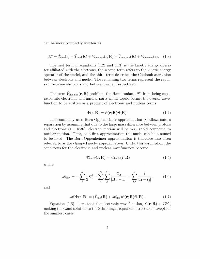
can be more compactly written as
H = Telec(r) + Tnuc(R) + Velec,nuc(r,R) + Vnuc,nuc(R) + Velec,elec(r). (1.3)
The first term in equations (1.2) and (1.3) is the kinetic energy opera-tor affiliated with the electrons, the second term refers to the kinetic energyoperator of the nuclei, and the third term describes the Coulomb attractionbetween electrons and nuclei. The remaining two terms represent the repul-sion between electrons and between nuclei, respectively.
The term Velec,nuc(r,R) prohibits the Hamiltonian, H , from being sepa-rated into electronic and nuclear parts which would permit the overall wave-function to be written as a product of electronic and nuclear terms
Ψ(r,R) = ψ(r; R)Θ(R). (1.4)
The commonly used Born-Oppenheimer approximation [8] allows such aseparation by assuming that due to the large mass difference between protonsand electrons (1 : 1836), electron motion will be very rapid compared tonuclear motion. Thus, as a first approximation the nuclei can be assumedto be fixed. The Born-Oppenheimer approximation is therefore also oftenreferred to as the clamped nuclei approximation. Under this assumption, theconditions for the electronic and nuclear wavefunction become
Helecψ(r; R) = Eelecψ(r; R) (1.5)
where
Helec = −N∑i
1
2∇2i −
N∑i
M∑A
ZA|RA − ri|
+N∑i,j
1
|ri − rj|, (1.6)
and
H Ψ(r,R) = (Tnuc(R) + Helec)ψ(r; R)Θ(R). (1.7)
Equation (1.6) shows that the electronic wavefunction, ψ(r; R) ∈ C3N ,making the exact solution to the Schrodinger equation intractable, except forthe simplest cases.
2
So far, we have omitted the requirement that, for a full description ofan electron, both its spatial, r and spin coordinates, ω must be specified,which are collectively termed x = {r, ω}. In the non-relativistic Schrodingerequation, however, the electronic Hamiltonian is independent of spin. In or-der to account for the spin dependence, two spin functions α(ω) and β(ω)are introduced. Furthermore, the constraint that identical particles are in-distinguishable has to be imposed. From this it follows, that many-electronwavefunctions must be antisymmetric with respect to the interchange of anytwo coordinates, xi and xj, often referred to as the antisymmetry or Pauliexclusion principle. In a mathematical context, this requirement is achievedby re-writing the wavefunction as (linear combinations of) Slater determi-nants [9, 10].
1.2 Wavefunction based Methods
1.2.1 Hartree-Fock Theory
The starting point for most wavefunction based approaches is the mean-field or Hartree-Fock approximation. This method employs a single Slaterdeterminant composed of one-electron spin orbitals, φi(xi), and defines thesimplest antisymmetric wavefunction for describing an N -electron system
ψHF(x1,x2, ...,xN) = |φ1(x1)φ2(x2) · · ·φN(xN)|. (1.8)
In order to derive the Hartree-Fock equations, the expectation value
EHF =〈ψHF|Helec|ψHF〉〈ψHF|ψHF〉
(1.9)
has to be minimized with respect to the spin orbitals φi(xi), subject to theconstraint that the orbitals remain orthonormal. In equation (1.9), Helec
denotes the electronic Hamiltonian (equation (1.6)).It has been shown [11], that the following eigenvalue equation provides
the solution to this constrained optimization problem:
f(x1)φi(x1) = εiφi(x1) (1.10)
with the one-electron Fock operator, f , and the energy of the ith orbital, εi.
3

Next, the set of orthonormal one-electron orbitals in equation (1.8) areexpanded in a known basis,
φi(x) =K∑µ
Cωµiχµ i = 1, 2, ..., K (1.11)
This expansion would be exact, if {χµ(r)} formed a complete set. However,in practice, only a small subset of Hilbert space is computationally feasibleand for molecular systems an atom-centered Gaussian basis is typically used.
Expansion in a basis allows the integro-differential equation shown in(1.10) to be written in matrix form as follows
F(C)C = SCε. (1.12)
where
Fµν = −1
2〈µ|∇2|ν〉+
nuc∑A
〈µ| 1
|RA − r||ν〉+
∑i
〈φiµ||φiν〉 (1.13)
Sµν = 〈µ|ν〉 (1.14)
〈pq||rs〉 =
∫ ∫φp(x1)φq(x2)
1
|x1 − x2|[φr(x1)φs(x2)− φs(x1)φr(x2)] (1.15)
and the diagonal matrix, ε, contains the orbital energies as entries. As indi-cated in equation (1.12), the so-called Roothaan-Hall equations [12, 13] arenonlinear and must be solved iteratively.
Although the Hartree-Fock approximation typically recovers more than99% of the total energy, the remaining 1% is crucial for quantitatively deter-mining relative energies and thus correctly predicting chemical events. Thedifference between the mean-field Hartree-Fock energy, EHF, and the exactnonrelativistic energy, Eexact, in a given (finite) basis defines the (basis set)correlation energy, Ecorr [14]:
Ecorr = Eexact − EHF (1.16)
4

In the following sections various different methods that attempt to re-cover the correlation energy will be discussed. In particular, the distinctionbetween weak and strong correlation problems will be made. In the for-mer case, the wavefunction can be described to a first approximation by theHartree-Fock wavefunction (cHF ≈ 0.9 or greater, equation (1.17))
|ψ〉 = cHF|ψHF〉+ ccorr|ψcorr〉 (1.17)
whereas in the strong correlation case this assumption will not hold andmultiple determinants will contribute considerably, or even equally.
1.2.2 Weak Correlation
1.2.2.1 Møller Plesset Perturbation Theory
Møller-Plesset perturbation theory derives from the Rayleigh-Schrodingermany-body perturbation theory (MBPT) [15, 16], in which the unperturbedzero-order wavefunction is the Hartree-Fock wavefunction [17]. If a singleconfiguration adequately approximates the full solution and the perturbationis small, the exact Hamiltonian H can be treated as a small perturbation, Vfrom the mean-field Hamiltonian, which is the sum of the one-electron Fockoperators (equation 1.19).
H |Ψi〉 = (H0 + λV )|Ψi〉 = Ei|Ψi〉 (1.18)
H0 =N∑i
f(i) (1.19)
Performing a Taylor series expansion of the exact eigenfunctions andeigenvalues in λ, yields
Ei =∞∑k=0
λkE(k)i (1.20)
and
|Ψi〉 =∞∑k=0
λk|Φ(k)i 〉 (1.21)
5
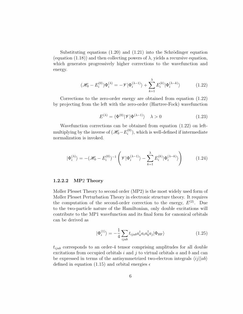
Substituting equations (1.20) and (1.21) into the Schrodinger equation(equation (1.18)) and then collecting powers of λ, yields a recursive equation,which generates progressively higher corrections to the wavefunction andenergy.
(H0 − E(0)i )Φ
(λ)i = −V |Φ(λ−1)
i 〉+λ∑k=1
E(k)i |Φ
(λ−k)i 〉 (1.22)
Corrections to the zero-order energy are obtained from equation (1.22)by projecting from the left with the zero-order (Hartree-Fock) wavefunction
E(λ) = 〈Φ(0)|V |Φ(λ−1)〉 λ > 0 (1.23)
Wavefunction corrections can be obtained from equation (1.22) on left-
multiplying by the inverse of (H0−E(0)i ), which is well-defined if intermediate
normalization is invoked.
|Φ(λ)i 〉 = −(H0 − E(0)
i )−1
(V |Φ(λ−1)
i 〉 −λ∑k=1
E(k)i |Φ
(λ−k)i 〉
)(1.24)
1.2.2.2 MP2 Theory
Møller Plesset Theory to second order (MP2) is the most widely used form ofMøller Plesset Perturbation Theory in electronic structure theory. It requiresthe computation of the second-order correction to the energy, E(2). Dueto the two-particle nature of the Hamiltonian, only double excitations willcontribute to the MP1 wavefunction and its final form for canonical orbitalscan be derived as
|Φ(1)i 〉 = −1
4
∑ijab
tijaba†aaia
†baj|ΦHF〉 (1.25)
tijab corresponds to an order-4 tensor comprising amplitudes for all doubleexcitations from occupied orbitals i and j to virtual orbitals a and b and canbe expressed in terms of the antisymmetrized two-electron integrals 〈ij||ab〉defined in equation (1.15) and orbital energies ε
6
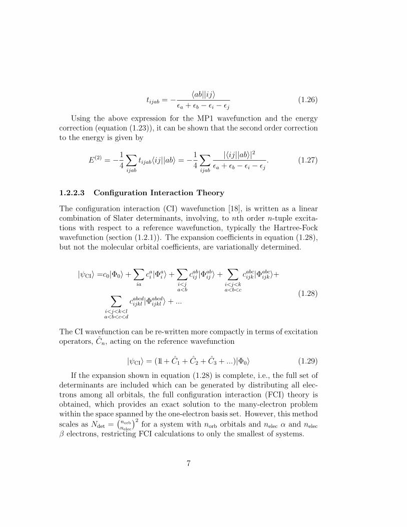
tijab = − 〈ab||ij〉εa + εb − εi − εj
(1.26)
Using the above expression for the MP1 wavefunction and the energycorrection (equation (1.23)), it can be shown that the second order correctionto the energy is given by
E(2) = −1
4
∑ijab
tijab〈ij||ab〉 = −1
4
∑ijab
|〈ij||ab〉|2
εa + εb − εi − εj. (1.27)
1.2.2.3 Configuration Interaction Theory
The configuration interaction (CI) wavefunction [18], is written as a linearcombination of Slater determinants, involving, to nth order n-tuple excita-tions with respect to a reference wavefunction, typically the Hartree-Fockwavefunction (section (1.2.1)). The expansion coefficients in equation (1.28),but not the molecular orbital coefficients, are variationally determined.
|ψCI〉 =c0|Φ0〉+∑ia
cai |Φai 〉+
∑i<ja<b
cabij |Φabij 〉+
∑i<j<ka<b<c
cabcijk |Φabcijk〉+
∑i<j<k<la<b<c<d
cabcdijkl |Φabcdijkl 〉+ ...
(1.28)
The CI wavefunction can be re-written more compactly in terms of excitationoperators, Cn, acting on the reference wavefunction
|ψCI〉 = (1 + C1 + C2 + C3 + ...)|Φ0〉 (1.29)
If the expansion shown in equation (1.28) is complete, i.e., the full set ofdeterminants are included which can be generated by distributing all elec-trons among all orbitals, the full configuration interaction (FCI) theory isobtained, which provides an exact solution to the many-electron problemwithin the space spanned by the one-electron basis set. However, this method
scales as Ndet =(norb
nelec
)2for a system with norb orbitals and nelec α and nelec
β electrons, restricting FCI calculations to only the smallest of systems.
7

Typically, one approximates the FCI expansion by including a limitedsubset of the excitation space, which gives rise to a hierarchy of methods, suchas configuration interaction singles (CIS, C1), configuration interaction sin-gles and doubles (CISD, C1+C2), etc. However, as for other weak-correlationmethods, the configuration interaction method when restricted to only thefirst few terms, requires that the reference wavefunction, |Φ0〉, is an adequateapproximation to |ψCI〉. Another major problem occurs in the configurationinteraction method, with the exception of FCI and CIS, is that it is not size-extensive [11].
In practice, two major forms of CI implementations exist. Spin- andspatially adapted configuration state functions (CSFs) [19] form the basis ofone of the methods, whereas the other involves Slater determinants [20–22].Although the former requires fewer terms, the latter is often used since con-siderable computational speed-ups are possible as the problem can be formu-lated in terms of vector-vector and matrix-vector algebra.
1.2.2.4 Coupled-Cluster Theory
In (single-reference) coupled-cluster (CC) theory, first introduced to the the-oretical chemistry community by Cizek and Paldus [23–27], the wavefunctionis represented in the form of a cluster expansion
|ψCC〉 = eT |ψ0〉 (1.30)
where |ψ0〉 typically refers to the HF wavefunction, and the cluster operatorT up to rank κ can be written as
T =N∑κ
Tκ (1.31)
with
Tκ =1
(n!)2
∑i,b
T b1,b2,...,bni1,i2,...,ina†bn ...a
†b1ai1 ...ain . (1.32)
Truncating operator in equation (1.31) yields methods such as coupled-cluster doubles, CCD, κ = 2 or coupled-cluster singles and doubles, CCSD,κ = 1, 2. In the case of the latter, often a perturbative triples correction,
8

indicated by (T ) is introduced. Today, CC defines one of the most suc-cessful and accurate correlated wavefunction approaches for single-referenceproblems [28]. In particular, the CCSD(T) [29, 30] approach has gained areputation as the ‘gold standard’ in quantum chemistry, because it produceshighly accurate energies. As a result of the exponential ansatz, CC theorypreserves size-extensivity, contrary to the CI method. Just as in the CI ap-proach, CC cannot describe strongly correlated systems without extendingthe excitation manifold to a computationally intractable length.
1.2.3 Strong Correlation Methods
Many problems encountered in chemistry feature electronic degeneracies ornear-degeneracies. These are referred to as multi-reference problems. Ex-amples include transition metals, bond dissociations, radicaloid systems andexcited states. (Near-)degeneracies lead to wavefunctions in which severaldeterminants contribute considerably, rather than just one. Since most elec-tronic structure methods are based on a single reference (c.f. sections 1.2.2.1,1.2.2.3, 1.2.2.4), systems featuring (near-)degeneracies continue to pose con-siderable challenges. Although some single-reference methods outlined in sec-tions 1.2.2.3 and 1.2.2.4 in principle could capture multi-reference character ifa sufficiently long expansion is used, this is typically not practical as the exci-tation level required would be intractably high. Therefore, many different al-ternative approaches have been developed to address the exponentially com-plex strong correlation problem. Noteworthy amongst these are the multi-configurational self-consistent field (MCSCF) approach and its variants, aswell as the density matrix renormalization group (DMRG) [31–38], valencebond methods, such as the spin-coupled (SC-VB) [39–41] and coupled-clustervalence bond (CC-VB) [42,43] theories. Also a broad class of methods existwhich attempt to describe strong correlation problems, but are based on asingle reference. The most pertinent methods to this thesis will be discussedin more detail in the following sections.
1.2.3.1 MCSCF, CASSCF and RASSCF
In multi-configurational self-consistent field (MCSCF) theory [44–49], boththe expansion coefficients, cI , as well as the corresponding orbital coefficients,C (section 1.2.1), are optimized self-consistently.
9

ψMCSCF =∑I
cIΦMCSCFI (1.33)
Here, the trial state function, ΦMCSCFI , may be a single Slater determi-
nant or a configuration state function (CSF). CSFs are spin- and, possibly,symmetry-adapted linear combinations of Slater determinants. If the sum inequation (1.33) consists of only one single Slater determinant, the expressionreduces to Hartree-Fock or mean field theory (section 1.2.1).
Contrary to the MCSCF approach, in which individual configurations areselected, in a complete active space SCF (CASSCF) [50, 51] calculation, anactive space is determined by choosing a set of active orbitals and electronsand forming all possible configurations in this subspace. By convention, theactive space is labelled as (nelec, norb). This corresponds to performing a fullconfiguration interaction (FCI) in the active space and thus the CASSCFmethod scales exponentially with the size of the active space. Although theideal active space would be spanned by all valence electrons, in practice, thisis unfeasible for most systems under consideration, as the largest active spacecurrently possible is (16,16) [52]. This constraint requires the user to select anorbital active space, which means the results may strongly depend on the cor-rect chemical intuition for the system under consideration [53]. Even worse,sometimes the physically correct active space is not computationally feasible.Especially, for constructing continuous and smooth potential energy surfacesthe correct choice of active space can pose considerable challenges. In orderto verify the adequacy of the active space in terms of its size and choice, atrial and error approach often becomes necessary. However, for many cases,demonstrating energy convergence with active space size is found to be chal-lenging due to practical limitations [54,55]. State-averaging [56,57], which isused to minimize root flipping [58] also appears as an issue in MCSCF andCASSCF calculations, since the number of states to average over is oftensomewhat arbitrary.
By definition, the CASSCF wavefunction incorporates all static correla-tion (at least if the appropriate active space is possible) [59]. In order torecover the missing dynamical correlation, which comprises the energy dif-ference between FCI and CASSCF [59], various different approaches havebeen applied, such as multi-reference CI (MRCI) [60], CASPT2 [61] and
10
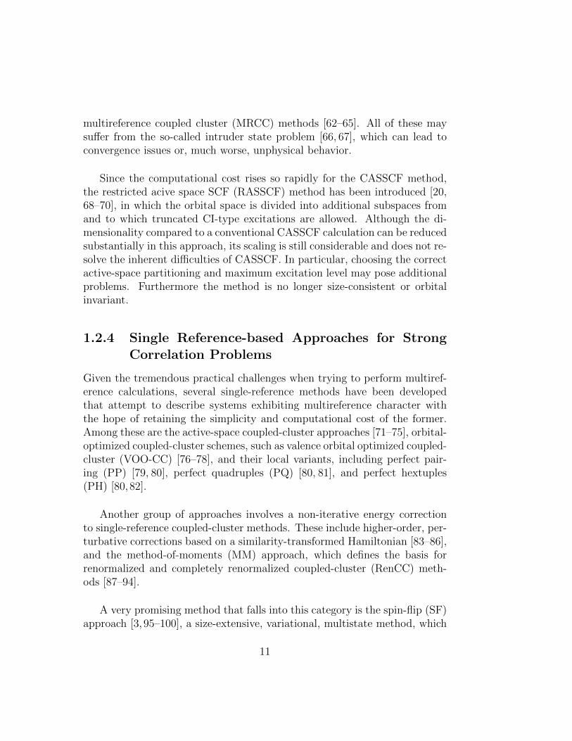
multireference coupled cluster (MRCC) methods [62–65]. All of these maysuffer from the so-called intruder state problem [66, 67], which can lead toconvergence issues or, much worse, unphysical behavior.
Since the computational cost rises so rapidly for the CASSCF method,the restricted acive space SCF (RASSCF) method has been introduced [20,68–70], in which the orbital space is divided into additional subspaces fromand to which truncated CI-type excitations are allowed. Although the di-mensionality compared to a conventional CASSCF calculation can be reducedsubstantially in this approach, its scaling is still considerable and does not re-solve the inherent difficulties of CASSCF. In particular, choosing the correctactive-space partitioning and maximum excitation level may pose additionalproblems. Furthermore the method is no longer size-consistent or orbitalinvariant.
1.2.4 Single Reference-based Approaches for StrongCorrelation Problems
Given the tremendous practical challenges when trying to perform multiref-erence calculations, several single-reference methods have been developedthat attempt to describe systems exhibiting multireference character withthe hope of retaining the simplicity and computational cost of the former.Among these are the active-space coupled-cluster approaches [71–75], orbital-optimized coupled-cluster schemes, such as valence orbital optimized coupled-cluster (VOO-CC) [76–78], and their local variants, including perfect pair-ing (PP) [79, 80], perfect quadruples (PQ) [80, 81], and perfect hextuples(PH) [80,82].
Another group of approaches involves a non-iterative energy correctionto single-reference coupled-cluster methods. These include higher-order, per-turbative corrections based on a similarity-transformed Hamiltonian [83–86],and the method-of-moments (MM) approach, which defines the basis forrenormalized and completely renormalized coupled-cluster (RenCC) meth-ods [87–94].
A very promising method that falls into this category is the spin-flip (SF)approach [3, 95–100], a size-extensive, variational, multistate method, which
11

can be extended to yield spin-eigenfunctions. In the spin-flip approach, ahigh-spin restricted open-shell Hartree-Fock (ROHF) reference is used as astarting point. The desired manifold is then accessed by spin-flipping. Bothsingle and double spin-flips have been explored within coupled cluster the-ory and in a RASSCF framework. The motivation behind the choice ofreference is that the appropriate high-spin wavefunction will be essentiallysingle-reference at all nuclear separations. This stands in contrast to theclosed-shell restricted wavefunction (RHF), which, as discussed, cannot ade-quately describe strong correlation problems. Furthermore, due to the Pauliexclusion principle, the dynamical correlation energy for same-spin electronswill be about an order of magnitude smaller than for opposite-spin elec-trons [101]. The improved description of the ground state reference alsostrongly influences the ability to correctly describe excitation energies [101].Besides this, the high-spin reference allows for an equal treatment of excitedand ground states. Also, contrary to e.g. CASSCF, the spin-flip method doesnot involve orbital optimizations and therefore avoids any attendant issues.Instead, orbital optimization is approximated through single excitations fromthe inactive spaces to the active space and vice versa. This allows the userto detect any inappropriate active space choices, which creates difficulty inCASSCF.
On the border between single- and multi-reference techniques lies a classof methods which makes use of a hybrid approach. In these approachesinformation from, e.g., valence-bond (VB) [102, 103], CASSCF [104] or CIcalculations, such as the important high-order cluster amplitudes, is used ina single-reference framework. Examples of such appraoches include the re-duced multireference coupled-cluster (RMRCC) method [105–110], and tai-lored CC [111,112]. Such methods, however, still depend on the success andcost of the initial multi-reference or VB calculations.
The unrestricted Hartree-Fock (UHF) method appears as the simplestamong all single-reference methods used for strong correlation. Although theenergetics often vastly improve by lifting the constraints of having the samespatial orbitals for α and β electrons, this approach often results in consid-erable spin contamination, which in turn can cause problems with propertycalculations [96]. Spin-projected methods have been introduced to removespin-contamination [113]. The so-called symmetry-projected Hartree-Fock-Bogoliubov (HFB) method has recently been implemented [114], which is
12
based on symmetry-breaking in an active space, followed by spin projection.The success of these methods, however, strongly depends on the amount ofspin contamination introduced.
1.3 Reduction of the Parameter Space
Including higher-order terms in the wavefunction expansions of MBPT, CI orCC, or increasing the number of electrons and orbitals in a CASSCF calcula-tion means that tensors of increasing order will enter the equations, causinga steep rise in computational cost and restricting such high-level calculationsto very small molecules. Even truncating the expansion at low order, theparameter space grows rapidly with the size of the molecule if no furtherconstraints are imposed. Thus, on the quest to push the limits of electronicstructure theory towards larger systems or more accurate treatments, low-parametric representations of the methods discussed above become essential.
The main basis for most of these approaches is to perform unitary orbitaltransformations so as to obtain a more compact description of the wavefunc-tion, which, upon truncation according to a certain parameter aims to max-imize the recovery in correlation energy. Often, such orbitals are determinedfrom computationally lower-scaling methods, such as MP2, and are subse-quently used to direct the choice of active space of higher-level methods, suchas the valence orbital optimized coupled-cluster (VOO-CC) method [76–78].
One research direction based on this concept focuses on exploiting wave-function locality [115]. The pioneering work by Pulay and Saebø, which com-bines the Boys [116] or Pipek-Mezey [117] localization schemes with numer-ical cutoffs determined by spatial distances, indicated substantial computa-tional savings with only small losses in numerical accuracy [115,118–121] andhas inspired local variants of MP2 [120, 122–124] and CC theory [125–128].Possible discontinuities in potential energy surfaces provide the main disad-vantage of this method [129–131]. Many researchers, including those in thegroups of Head-Gordon [130–135] and Scuseria [136,137] have formulated al-ternative theories to address this issue.
The other main school of thought restricts the excitation level withina certain orbital active space. Besides the aforementioned trial-and-error
13

approach guided by the user’s chemical intuition (section 1.2.3.1), many dif-ferent attempts have been made to determine how to most efficiently truncatethe orbital active space using quantitative descriptors. These mainly focuson the compression of the virtual space. The oldest and most commonly en-countered technique forms natural orbitals by diagonalizing the one-particledensity matrix of a particular method. The resulting eigenvalues, also knownas occupation numbers, lie between 0 and 1. These determine the importanceof the corresponding orbital. This often allows truncation of the virtualspace by up to 50%, yet only introducing errors of < 1 kcal/mol. In thefrozen natural orbital (FNO) approach, the virtual orbitals to be retainedin a CC [138–140], optimized doubles (OD) [76–78], or QCISD calculation,are obtained from the virtual-virtual block of the MP2 density, which scalesas O(N5). Recently, this method has been extended to ionized systems (IP-CC) [141]. After determining the FNOs, the final subset of virtual orbitalsare selected by specifying the percentage of the full space to be included(percentage of virtual orbitals, POVO) [139, 140] or by requiring the accu-mulative natural orbital occupation number to lie above a certain thresholdcompared the total number of electrons in the system under consideration(occupation threshold, OCCT) [141]. The resulting computational speed-upwill be 1/(1 − n)N , where n defines the fraction of the full virtual space re-tained in the calculation and the method scales as N .
Other commonly used forms of natural orbitals approximate the pair-natural orbitals, PNO [18, 142–145] (formerly known as pseudo-natural or-bitals [146]). These maximize the interaction of a pair of occupied orbitalswith a linear combination of virtual ones, which is equivalent to forming thenatural orbitals for this specific pair. This procedure introduces localizationwithout the need of selecting spatial domains. Another approach involvesoptimization of the virtual spaces (OVOS) [147–149] to select important vir-tual orbitals. In this approach, the virtual orbitals are divided into an activeand inactive space and the transformation of basis is achieved by performingself-consistent orbital rotations between those two subspaces through invok-ing the Hylleraas functional.
Besides these two main classes, there are several other approaches whichutilize mathematical rather than physical insight in order to reduce the com-putational cost. These include matrix or tensor decomposition methods,such as the Cholesky factorization [150–157], the resolution-of-the-identity
14
approach, also known as density fitting [158, 159], the Laplace transforma-tion [136,160–168], and methods based on matrix or tensor sparsity.
1.4 Density Functional Theory
Density functional theory (DFT) ranks as the most commonly used alterna-tive to wavefunction-based methods and today about 80-90% of all electronicstructure calculations use this approach. Although, unlike wavefunctionbased methods, density functional theory cannot be systematically improved,it often becomes the only available method for large systems due to its low-scaling computational cost (O(N3)). The Hohenberg-Kohn theorems [169]form the theoretical basis for density functional theory. Introduction of theKohn-Sham equations, which use the idea of expressing the problem as afictitious system of non-interacting electrons in an effective potential [170]then made this method viable.
Although the theory is formally exact, the form of the exact exchange-correlation functional is unknown and therefore numerous flavors of densityfunctionals exist to approximate it. Often, the different types of exchange-correlation functionals get grouped according to the so-called ‘Jacob’s lad-der’: local density approximation, LDA, generalized gradient approximation,GGA, that depend on the spin densities and their reduced gradient, the meta-GGAs described via the spin kinetic energy density, the hybrid functionalswhich contain a fraction of exact exchange, range-separated functionals anddouble-hybrids where the DFT orbitals are used in a non-self-consistent MP2-type correction.
Amongst these, the hybrid functional B3LYP [171] is still one of the mostwidely used functionals, despite its known drawbacks of inadequately describ-ing Rydberg [172–176] and charge-transfer excited states [177, 178], barrier-heights [179], and bond dissociation processes due to the self-interaction er-ror [180]. Different attempts have been made to partially resolve this is-sue [180–182], with one promising strategy being the development of range-separated functionals [183–191]. Their inability to describe dispersion inter-actions creates another limitation of most functionals. The simplest way tocorrect for this failure are the −D [192–194] and −XDM corrections [195].However, more elaborate schemes have also been proposed [196].
15
Furthermore, due to the linear response formalism in time-dependentDFT (TDDFT), these methods cannot capture excitations featuring pre-dominantly doubly excited character [176, 197], which become crucial in ex-plaining various phenomena, for example, the singlet fission process [198,199].
Although DFT describes dynamic correlation fairly well, strongly-correlatedsystems pose considerable challenges to DFT [200], as the reference is asingle Slater determinant. Recently, Grimme and Cremer proposed a com-bined DFT/multireference approach, in which DFT orbitals are used in anMRCI [201] or CASSCF [200] calculation to address this issue. Of course,such approaches will not reduce the inherent problems of multi-referencemethods (section 1.2.3.1).
16

Chapter 2
Higher Order Singular ValueDecomposition (HOSVD) inQuantum Chemistry
Higher Order Singular Value Decomposition (HOSVD) is studied in the con-text of quantum chemistry, with particular focus on the decomposition of theT2 amplitudes obtained from second order Møller Plesset Perturbation (MP2)theory calculations. Our test calculations reveal that HOSVD transformedamplitudes yield considerably faster convergence in MP2 correlation energy,both in terms of amplitude and orbital truncation. Also, HOSVD orbitalsdisplay increased bonding/antibonding character compared to Hartree-Fock(HF) orbitals. In contrast to canonical MP2 theory, the leading amplitudesare those between corresponding occupied-virtual orbital pairs. The HOSVDorbitals are paired up automatically around the Fermi level in decreasing im-portance, so that the strongest occupied virtual pair are the Highest Occu-pied Molecular Orbital and Lowest Unoccupied Molecular Orbital (HOMO-LUMO). We show that in the case of MP2 amplitudes, the HOSVD orbitalsare equivalent to the unrelaxed MP2 natural orbitals.
The least squares Higher Orthogonal Iteration (HOOI) algorithm yieldsonly minor improvements over the sub-optimal truncated orbital space ob-tained from the HOSVD.
17

2.1 Introduction
2.1.1 Motivation
Decomposition of multilinear arrays has important applications in numerousfields, such as signal processing [202–204], graph analysis [205–207], numeri-cal analysis [208–212], neuroscience [213–216] and computer vision [217–220].
In Quantum Chemistry, higher order tensors arise for example in thewavefunction-based description of electron correlation and are an essentialpart of any state-of-the-art wavefunction based calculation [221]. However,the total number of elements in an array grows exponentially with the num-ber of indices. This problem, known as the “curse of dimensionality” [222],restricts high-level calculations to molecules comprised of only a handful ofatoms. Low-parametric representations of multilinear arrays have the poten-tial of making such computations accessible to larger systems. In addition,such a compact representation may lend itself to natural truncations andthus novel active space methods [51, 77]. Despite great progress, for exam-ple [208], there is still room for improvement and it may be advantageous toconsider the problem from the perspective of numerical analysis.
Tensor decompositions may also be useful in data analysis. Multiple in-dex quantities are difficult to interpret and thus a one-particle description isdesirable to aid physical understanding [223–225].
In this chapter, we investigate the applicability of the Higher Order Sin-gular Value decomposition (HOSVD), a multilinear generalization of the sin-gular value decomposition (SVD) towards novel active space methods. In afirst attempt we apply this method to the MP2 T2 tensor.
The chapter is structured as follows: In the first part we give a briefoverview of the most important tensor decompositions before discussing theHOSVD in more detail in sections 2 (Theory) and 3 (Results).
2.1.2 Notation and Basic Definitions
The following notation will be used throughout the chapter: scalars are indi-cated by lower-case letters (a, b, ...;α, β, ...), vectors are denoted as capitals(A,B, ...) (italic shaped), matrices are written in bold-face capitals (A,B,
18

...), and tensors are indicated as calligraphic capitals (A,B,...). The only ex-ceptions are indices indicating upper bounds. For these cases, the followingletters are reserved: I, P,Q,R.
A tensor with d indices will be referred to as a d-mode tensor or an order-dtensor.
The scalar product 〈A,B〉 of two tensors A,B ∈ RI1×I2×...×Id is given as
〈A,B〉 def=∑i1
∑i2
...∑id
b∗i1i2...idai1i2...id (2.1)
in which * denotes the complex conjugate.
The Frobenious norm of a tensor A, ||A||F is defined as
||A||Fdef=√〈A,A〉 (2.2)
The n-mode product A×n U of a tensor A ∈ RI1×I2×...×Id with a matrixU ∈ RJn×In is an (I1×I2× ...×In−1×Jn×In+1× ...×Id) tensor with entries:
(A×n U)i1i2...in−1jnin+1...iddef=∑in
ai1i2...in−1inin+1...idujnin (2.3)
The outer product, denoted by ◦, defines the following operation:
(U (1) ◦ U (2) ◦ ... ◦ U (d))i1i2...iddef= U
(1)i1U
(2)i2...U
(d)id
∀ in ∈ {1, ..., In}(2.4)
2.1.3 Overview of Tensor Decompositions and TheirRelation to Quantum Chemistry
Tensor decompositions can be divided into two main classes. The first isreferred to as Tucker decomposition or principal component analysis [226–231], and takes the following form for a d-mode tensor:
T def= S ×1 U(1) ×2 U(2) ×3 ...×d U(d) =
=P∑p=1
Q∑q=1
...
R∑r=1
spq...rU(1)p ◦ U (2)
q ◦ ... ◦ U (d)r
(2.5)
19

Here, the original tensor T is decomposed into the core-tensor S andmatrices U(n). The latter are known as Tucker factors or mode factors, whichact on the ith mode of S. If orthogonality constraints are introduced, thismethod is known as Higher-Order Singular Value Decomposition (HOSVD)or multilinear SVD [232].
In the context of quantum chemistry the Tucker decomposition may belinked to the complete active space self-consistent field (CASSCF) method[51]. Decomposition of amplitudes corresponding to a specific level of exci-tation yields optimized orbitals for each of these tensors. However, if theseTucker factors are optimized under the constraint that all of the mode factorshave to be the same, the CASSCF transformation matrices are obtained.
The second tensor decomposition is known as CANDECOMP/PARAFAC(CP) [233–239]. This approach approximates a tensor as a sum of Kroneckerproducts of rank-one tensors:
T def=
R∑r=1
U (1)r ◦ U (2)
r ◦ ... ◦ U (d)r (2.6)
Here, the number of summands R is called the canonical rank. It is oftenassumed that the columns of U(i) are normalized to length 1 and the vectorΛ absorbs the corresponding weights:
T =R∑r=1
ΛrU(1)r ◦ U (2)
r ◦ ... ◦ U (n)r (2.7)
This form reveals that CP can be regarded as a special case of the Tuckerdecomposition, provided the core tensor is superdiagonal and P = Q = ... =R.
The relationship to quantum chemistry can be drawn by noting that thefull configuration interaction (FCI) method can be seen as a CP decompo-sition. In particular, the perfect pairing (PP) approach [240–242] can beviewed as a mode-1 approximation to the FCI tensor, as described in equa-tion (7), i.e.:
T PP =R∑r=1
ΛrU(1)r (2.8)
20
since the associated PP excitation operator takes the form:
T PP2 |Φ0〉 =
∑i
ti |Φi〉 (2.9)
Here |Φi〉 is the determinant |Φ0〉 with the occupied pair φiφi replaced by theunoccupied (correlating) pair φ∗i φ
∗i .
Comparison of the CP and Tucker decompositions from a numericalstandpoint reveals that the canonical rank reduction is an unstable problemand none of the current algorithms can perform a reliable rank reductiongiven a prescribed accuracy [243], which is also known as recompression.There have been some advances in this field [208, 244, 245], however, thecanonical rank has to be known or guessed in advance. In addition, conver-gence may be slow [246].
On the other hand, the corresponding Tucker approach can be performedwith the reliability of the well-understood singular value decomposition (SVD).This makes the HOSVD a preferable candidate for active space techniques,especially since algorithms have been devised which determine the reducedtensor dimension automatically [247].
The Tucker decomposition, however, also has a disadvantage comparedto the CP approach; the cost scales exponentially with the number of modes,d. This is due to the core tensor, which contains Rd elements (if P = Q =... = R). At first glance the number of parameters in a CP decomposition(d · R · n + R) does not seem to suffer from this exponential dependence.However, R is found to increase rapidly and often depends on d exponen-tially [248]. In order to overcome memory issues, so-called cross approxima-tion techniques have been introduced [249–254], which make Tucker approx-imations feasible even for tensors with d ≥ 1000.
We are interested in studying this method in more detail, in light ofthe potential applications of HOSVD in quantum chemistry, in particularin Coupled-Cluster (CC) methods [255], many-body perturbation theory(MBPT) [256] or active-space approaches. Specifically, we analyzed decom-posed and rank truncated T2 tensors, which were obtained from MP2 calcu-lations. We were also able to show the connection between HOSVD T2 andMP2 natural orbitals.
21

2.2 Theory
2.2.1 Review of HOSVD without any numerical ap-proximations such as rank truncation (untrun-cated HOSVD)
The HOSVD is defined for complex tensors [257]. However, in the applica-tions under consideration, all tensors are real-valued and the correspondingnotations are adapted accordingly.
The main steps of the untruncated HOSVD are1.) Matricization (unfolding) of the mode-d tensor T ∈ RI1×I2×...×Id yields dmatrices, A(1), ...,A(d); A(n) ∈ RIn×(I1I2...In−1In+1...Id). Thereby, tensor element(T )i1,i2,...,id maps to matrix element (A(n))in,j(n) where
j(n) = in+1In+2In+3...IdI1I2...Id−1+
in+2In+3In+4...IdI1I2...Id−1 + ...
+ idI1I2...Id−1 + i1I2I3...In−1 + ...+ in−1
(2.10)
for in = 0, 1, ..., In − 1.
2.) Determining the d left singular matrices, U(1), ...,U(d)
A(n) = U(n)Σ(n)V(n)T for n = 1, ..., d (2.11)
where U(n) ∈ RIn×In . Σ(n) ∈ RIn×(I1I2...In−1In+1..Id) is a diagonal matrix,featuring the singular values in descending order and V(n) are the right sin-gular matrices. The singular matrices are orthonormal: U(n)TU(n) = 1 andV(n)TV(n) = 1.
3.) Determining the (compressed) core tensor, S ∈ RI1×I2×...×Id by contract-ing the original tensor T with the left singular matrices U(n) obtained in step2:
S = T ×1 U(1)T ×2 U(2)T ...×d U(d)T (2.12)
A pseudocode HOSVD algorithm is shown in Fig. 2.1.
One of the properties of the subtensors Sin=α of S ∈ RI1×I2×..×Id (whichare obtained by fixing the nth index to α) is ordering:
22
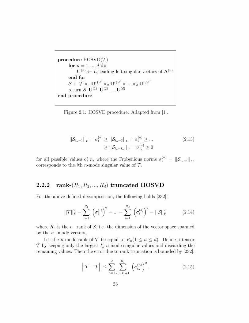
procedure HOSVD(T )for n = 1, ..., d do
U(n) ← In leading left singular vectors of A(n)
end for
S ← T ×1 U(1)T ×2 U(2)T × ...×d U(d)T
return S,U(1),U(2), ...,U(d)
end procedure
Figure 2.1: HOSVD procedure. Adapted from [1].
||Sin=1||F = σ(n)1 ≥ ||Sin=2||F = σ
(n)2 ≥ ... (2.13)
≥ ||Sin=In||F = σ(n)In≥ 0
for all possible values of n, where the Frobenious norms σ(n)i = ||Sin=i||F ,
corresponds to the ith n-mode singular value of T .
2.2.2 rank-(R1, R2, ..., Rd) truncated HOSVD
For the above defined decomposition, the following holds [232]:
||T ||2F =
R1∑i=1
(σ
(1)i
)2
= ... =
Rd∑i=1
(σ
(d)i
)2
= ||S||2F (2.14)
where Rn is the n−rank of S, i.e. the dimension of the vector space spannedby the n−mode vectors.
Let the n-mode rank of T be equal to Rn(1 ≤ n ≤ d). Define a tensorT by keeping only the largest I ′n n-mode singular values and discarding theremaining values. Then the error due to rank truncation is bounded by [232]:
∣∣∣∣∣∣T − T ∣∣∣∣∣∣ ≤ d∑n=1
R1∑i1=I′1+1
(σ
(n)in
)2
. (2.15)
23
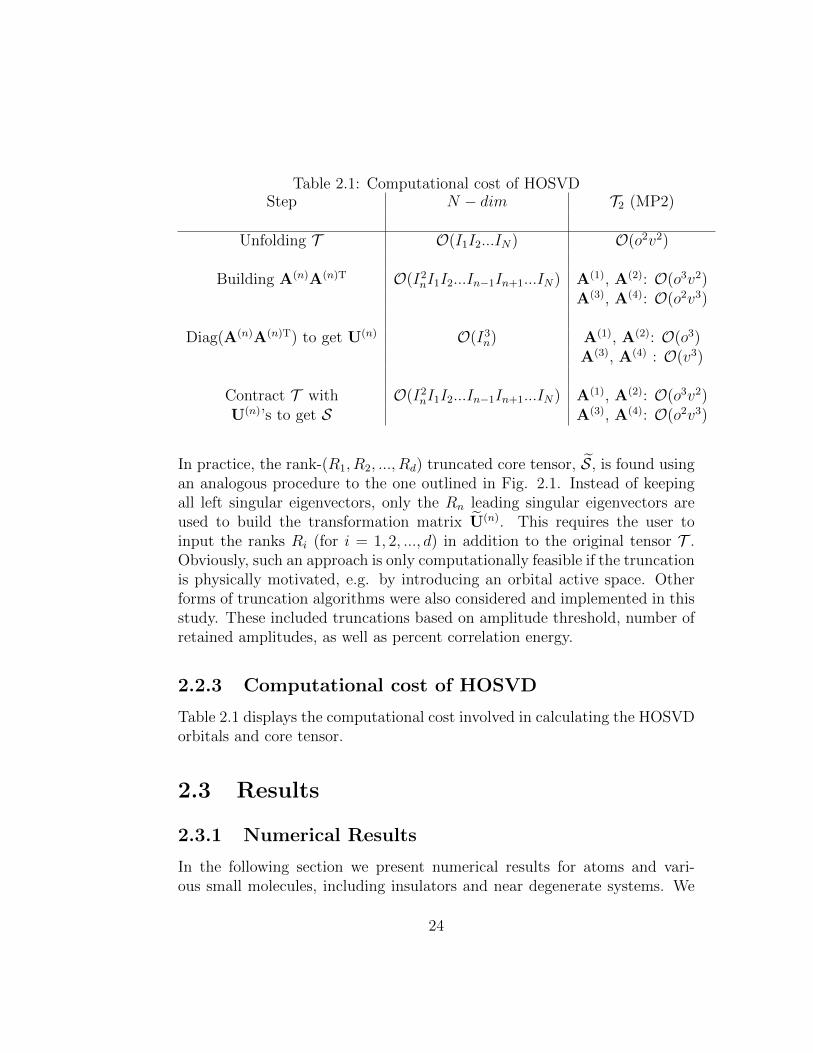
Table 2.1: Computational cost of HOSVDStep N − dim T2 (MP2)
Unfolding T O(I1I2...IN) O(o2v2)
Building A(n)A(n)T O(I2nI1I2...In−1In+1...IN) A(1), A(2): O(o3v2)
A(3), A(4): O(o2v3)
Diag(A(n)A(n)T) to get U(n) O(I3n) A(1), A(2): O(o3)
A(3), A(4) : O(v3)
Contract T with O(I2nI1I2...In−1In+1...IN) A(1), A(2): O(o3v2)
U(n)’s to get S A(3), A(4): O(o2v3)
In practice, the rank-(R1, R2, ..., Rd) truncated core tensor, S, is found usingan analogous procedure to the one outlined in Fig. 2.1. Instead of keepingall left singular eigenvectors, only the Rn leading singular eigenvectors areused to build the transformation matrix U(n). This requires the user toinput the ranks Ri (for i = 1, 2, ..., d) in addition to the original tensor T .Obviously, such an approach is only computationally feasible if the truncationis physically motivated, e.g. by introducing an orbital active space. Otherforms of truncation algorithms were also considered and implemented in thisstudy. These included truncations based on amplitude threshold, number ofretained amplitudes, as well as percent correlation energy.
2.2.3 Computational cost of HOSVD
Table 2.1 displays the computational cost involved in calculating the HOSVDorbitals and core tensor.
2.3 Results
2.3.1 Numerical Results
In the following section we present numerical results for atoms and vari-ous small molecules, including insulators and near degenerate systems. We
24
carried out computations with several Pople and Dunning style basis sets.
1,0E-16
1,0E-14
1,0E-12
1,0E-10
1,0E-08
1,0E-06
1,0E-04
1,0E-02
1,0E+00
1 10 100 1000
log(#Amplitudes)
log(
Am
plitu
de M
agni
tude
)
HOSVD
Original
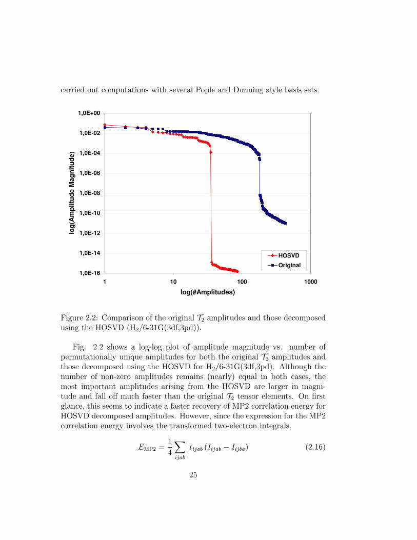
Figure 2.2: Comparison of the original T2 amplitudes and those decomposedusing the HOSVD (H2/6-31G(3df,3pd)).
Fig. 2.2 shows a log-log plot of amplitude magnitude vs. number ofpermutationally unique amplitudes for both the original T2 amplitudes andthose decomposed using the HOSVD for H2/6-31G(3df,3pd). Although thenumber of non-zero amplitudes remains (nearly) equal in both cases, themost important amplitudes arising from the HOSVD are larger in magni-tude and fall off much faster than the original T2 tensor elements. On firstglance, this seems to indicate a faster recovery of MP2 correlation energy forHOSVD decomposed amplitudes. However, since the expression for the MP2correlation energy involves the transformed two-electron integrals,
EMP2 =1
4
∑ijab
tijab (Iijab − Iijba) (2.16)
25

we have also tested the performance of the HOSVD amplitudes when con-tracted to the MP2 energy.
The percent contribution to the MP2 correlation energy for the n largestamplitudes was computed for both the original T2 tensor and the HOSVDdecomposed analogue. Since the transformation matrices obtained fromHOSVD act on the occupied and virtual space separately (i.e. there areno orbital rotations that cause mixing of the occupied and virtual space),the overall density and therefore the energy is the same as for canonicalMP2. This allows direct comparison of the correlation energy values for thetwo methods. Figs. 2.3 and 2.4 show the percent correlation energy recoveryfor H2 in various basis sets.
H2,6-31G**
1
2
3
5
6
1
2
37
8 9 1013 15 17
4 56 7 8 9
0
20
40
60
80
100
0 2 4 6 8 10 12 14 16 18
#Amplitudes included
%M
P2
Cor
rela
tion
Ene
rgy
OriginalHOSVD
Figure 2.3: Percent MP2 correlation energy vs. number of amplitudes in-cluded (H2/6-31G**)
26

H2,6-31++G**
1
2
3
5
6
1
2
37
28262321201917151413129
29
114 5
6 7 8 9 10 11
0
20
40
60
80
100
0 5 10 15 20 25 30 35
#Amplitudes included
%M
P2
Cor
rela
tion
Ene
rgy
OriginalHOSVD
Figure 2.4: Percent MP2 correlation energy vs. number of amplitudes in-cluded (H2/6-31++G**)
We also calculated compression factors γOrig/HOSVD for various systemsand basis sets (Tables 2.2 and 2.3). The compression factor γOrig/HOSVD isdefined as the ratio of original and HOSVD decomposed amplitudes neces-sary to reach a given percentage of correlation energy. This allows compactcomparison of the correlation energy convergence between the two represen-tations. Since the HOSVD is performed on amplitudes, this approach is notexpected to yield an optimal convergence of the correlation energy.
In almost all cases considerably fewer HOSVD transformed amplitudesare required to obtain a certain amount of correlation energy, even for 99 per-cent correlation energy recovery. The main exceptions are CH4 (cc-pVDZ)and Ne (6-311G).
In general, addition of diffuse basis functions results in higher compression
27
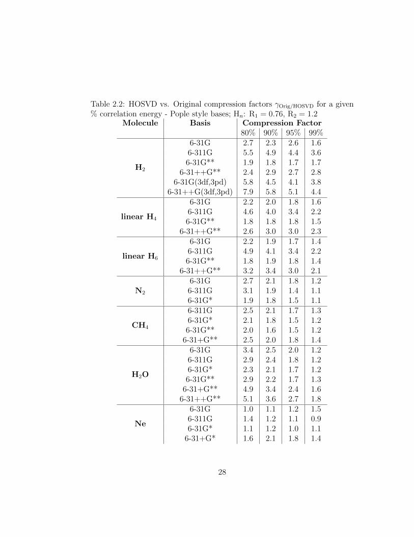
Table 2.2: HOSVD vs. Original compression factors γOrig/HOSVD for a given% correlation energy - Pople style bases; Hn: R1 = 0.76, R2 = 1.2
Molecule Basis Compression Factor80% 90% 95% 99%
H2
6-31G 2.7 2.3 2.6 1.66-311G 5.5 4.9 4.4 3.66-31G** 1.9 1.8 1.7 1.7
6-31++G** 2.4 2.9 2.7 2.86-31G(3df,3pd) 5.8 4.5 4.1 3.8
6-31++G(3df,3pd) 7.9 5.8 5.1 4.4
linear H4
6-31G 2.2 2.0 1.8 1.66-311G 4.6 4.0 3.4 2.26-31G** 1.8 1.8 1.8 1.5
6-31++G** 2.6 3.0 3.0 2.3
linear H6
6-31G 2.2 1.9 1.7 1.46-311G 4.9 4.1 3.4 2.26-31G** 1.8 1.9 1.8 1.4
6-31++G** 3.2 3.4 3.0 2.1
N2
6-31G 2.7 2.1 1.8 1.26-311G 3.1 1.9 1.4 1.16-31G* 1.9 1.8 1.5 1.1
CH4
6-311G 2.5 2.1 1.7 1.36-31G* 2.1 1.8 1.5 1.26-31G** 2.0 1.6 1.5 1.2
6-31+G** 2.5 2.0 1.8 1.4
H2O
6-31G 3.4 2.5 2.0 1.26-311G 2.9 2.4 1.8 1.26-31G* 2.3 2.1 1.7 1.26-31G** 2.9 2.2 1.7 1.3
6-31+G** 4.9 3.4 2.4 1.66-31++G** 5.1 3.6 2.7 1.8
Ne
6-31G 1.0 1.1 1.2 1.56-311G 1.4 1.2 1.1 0.96-31G* 1.1 1.2 1.0 1.1
6-31+G* 1.6 2.1 1.8 1.4
28

Table 2.3: HOSVD vs. Original compression factors γOrig/HOSVD for a given% correlation energy - Dunning style bases; Hn: R1 = 0.76, R2 = 1.2
Molecule Basis Compression Factor80% 90% 95% 99%
H2
cc-pVDZ 2.1 2.3 2.0 1.8aug-cc-pVDZ 5.7 6.6 5.7 5.1
cc-pVTZ 5.0 3.7 3.4 3.0
linear H4
cc-pVDZ 2.0 2.1 2.0 1.7aug-cc-pVDZ 6.7 6.3 5.4 3.2
cc-pVTZ 5.6 4.0 3.3 2.3
linear H6
cc-pVDZ 2.3 2.2 2.0 1.5aug-cc-pVDZ 7.4 6.6 5.4 3.4
cc-pVTZ 5.6 4.0 3.1 2.1
N2
cc-pVDZ 1.6 1.5 1.4 1.2aug-cc-pVDZ 4.7 3.9 3.3 1.9
cc-pVTZ 2.3 1.6 1.4 1.1
CH4cc-pVDZ 1.4 0.9 0.7 0.5
aug-cc-pVDZ 4.8 3.3 2.3 1.3
H2Occ-pVDZ 3.3 2.5 1.9 1.4
aug-cc-pVDZ 8.2 5.7 4.2 2.5cc-pVTZ 5.2 4.0 2.9 1.9
Ne
cc-pVDZ 1.0 1.0 1.1 1.2aug-cc-pVDZ 3.4 3.0 2.4 1.6
cc-pVTZ 1.6 1.4 1.3 1.1aug-cc-pVTZ 3.1 2.8 2.2 1.5
29
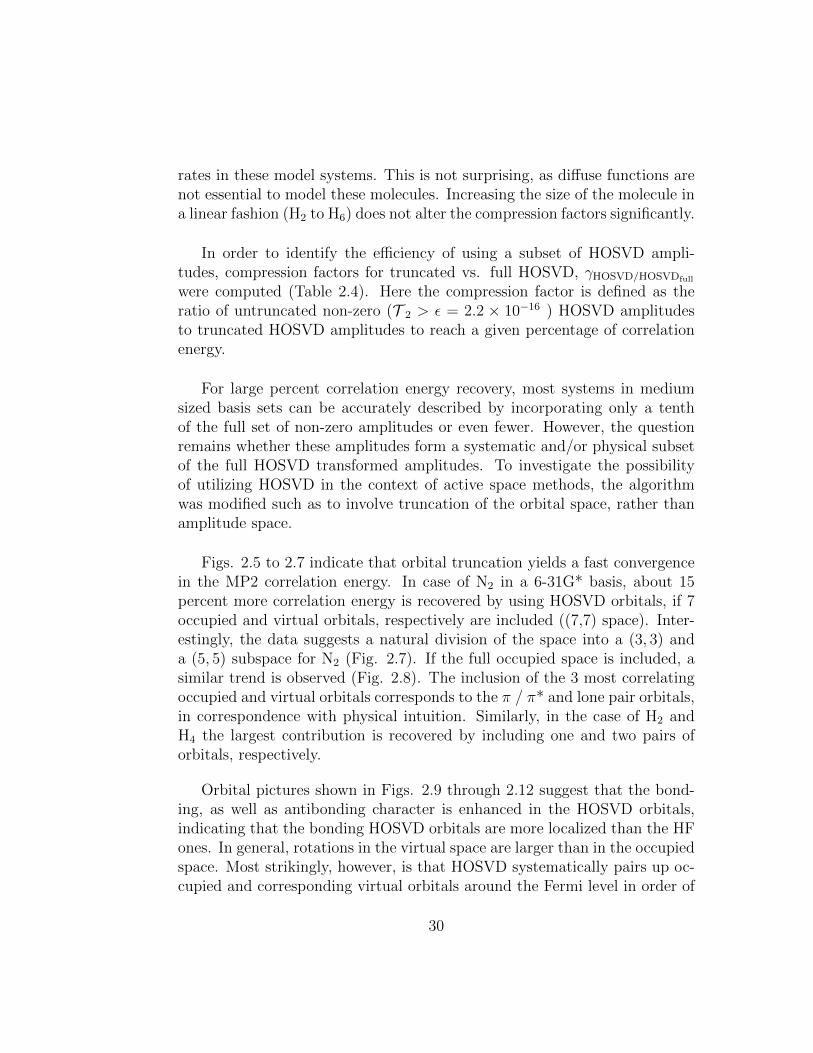
rates in these model systems. This is not surprising, as diffuse functions arenot essential to model these molecules. Increasing the size of the molecule ina linear fashion (H2 to H6) does not alter the compression factors significantly.
In order to identify the efficiency of using a subset of HOSVD ampli-tudes, compression factors for truncated vs. full HOSVD, γHOSVD/HOSVDfull
were computed (Table 2.4). Here the compression factor is defined as theratio of untruncated non-zero (T 2 > ε = 2.2 × 10⁻¹⁶ ) HOSVD amplitudesto truncated HOSVD amplitudes to reach a given percentage of correlationenergy.
For large percent correlation energy recovery, most systems in mediumsized basis sets can be accurately described by incorporating only a tenthof the full set of non-zero amplitudes or even fewer. However, the questionremains whether these amplitudes form a systematic and/or physical subsetof the full HOSVD transformed amplitudes. To investigate the possibilityof utilizing HOSVD in the context of active space methods, the algorithmwas modified such as to involve truncation of the orbital space, rather thanamplitude space.
Figs. 2.5 to 2.7 indicate that orbital truncation yields a fast convergencein the MP2 correlation energy. In case of N2 in a 6-31G* basis, about 15percent more correlation energy is recovered by using HOSVD orbitals, if 7occupied and virtual orbitals, respectively are included ((7,7) space). Inter-estingly, the data suggests a natural division of the space into a (3, 3) anda (5, 5) subspace for N2 (Fig. 2.7). If the full occupied space is included, asimilar trend is observed (Fig. 2.8). The inclusion of the 3 most correlatingoccupied and virtual orbitals corresponds to the π / π* and lone pair orbitals,in correspondence with physical intuition. Similarly, in the case of H2 andH4 the largest contribution is recovered by including one and two pairs oforbitals, respectively.
Orbital pictures shown in Figs. 2.9 through 2.12 suggest that the bond-ing, as well as antibonding character is enhanced in the HOSVD orbitals,indicating that the bonding HOSVD orbitals are more localized than the HFones. In general, rotations in the virtual space are larger than in the occupiedspace. Most strikingly, however, is that HOSVD systematically pairs up oc-cupied and corresponding virtual orbitals around the Fermi level in order of
30

Table 2.4: HOSVD compression factors, γHOSVD/HOSVDfullfor a given percent
correlation energy - Dunning bases; Hn: R1 = 0.76, R2 = 1.2Molecule Basis Compression Factor
80% 90% 95% 99%
H2
cc-pVDZ 2.6 2.3 1.5 1.1aug-cc-pVDZ 12.9 10.0 6.9 4.7
cc-pVTZ 12.5 6.3 4.2 2.5aug-cc-pVTZ 57.8 28.0 18.5 10.5
linear H4
cc-pVDZ 44.4 29.5 21.0 12.0aug-cc-pVDZ 150.0 91.1 59.0 24.0
cc-pVTZ 262.3 108.5 63.2 27.6
linear H6
cc-pVDZ 57.2 34.4 23.2 11.5aug-cc-pVDZ 187.9 105.3 64.2 25.0
cc-pVTZ 320.3 138.7 75.0 30.6
N2
cc-pVDZ 40.1 21.0 13.3 5.9aug-cc-pVDZ 156.5 76.4 43.7 13.1
cc-pVTZ 77.6 28.3 14.9 6.8
CH4cc-pVDZ 43.6 18.1 10.2 4.5
aug-cc-pVDZ 163.5 67.0 34.8 11.6
H2Occ-pVDZ 82.5 39.1 21.6 9.5
aug-cc-pVDZ 285.6 116.9 60.0 20.9cc-pVTZ 171.1 67.3 32.3 12.3
Ne
cc-pVDZ 52.3 36.5 25.7 12.1aug-cc-pVDZ 222.1 125.7 65.9 22.2
cc-pVTZ 102.8 51.3 30.7 13.7aug-cc-pVTZ 242.2 122.2 64.6 23.5
31
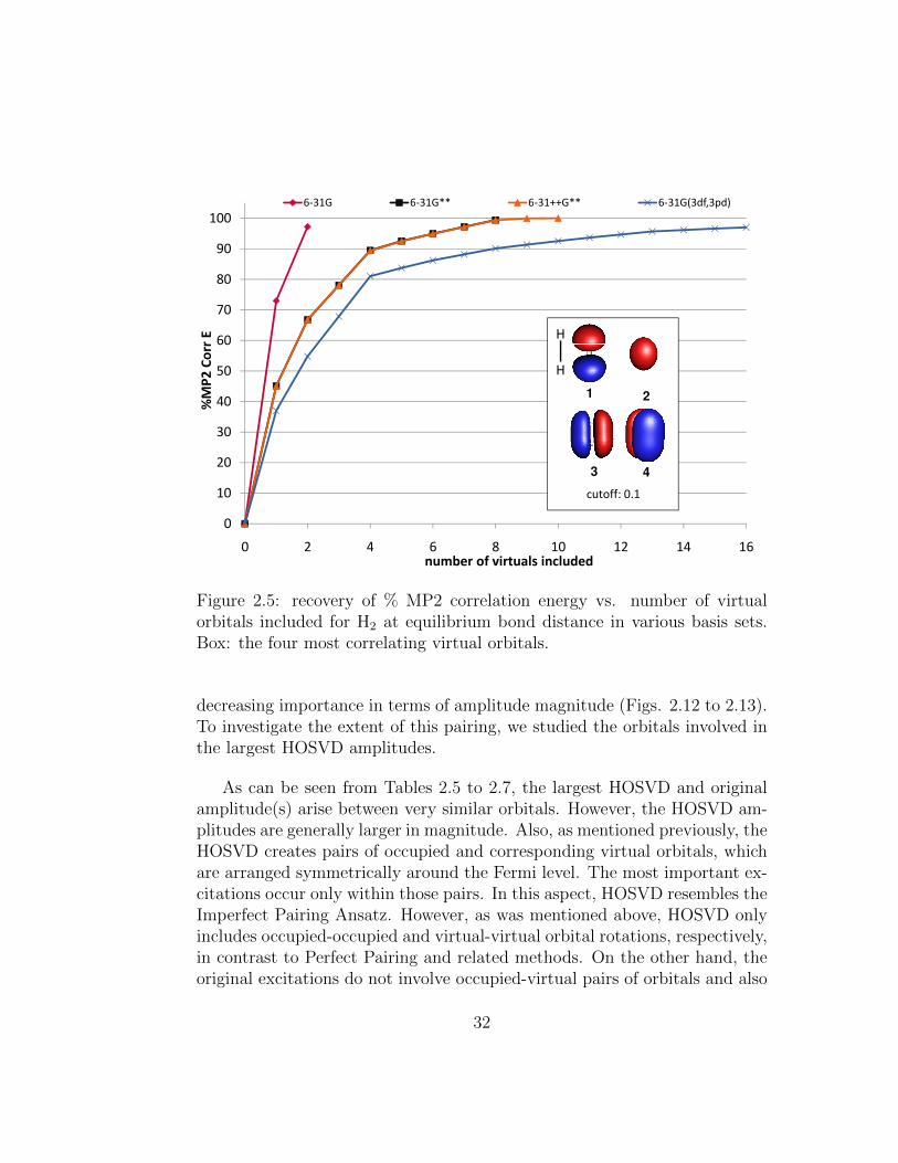
40
50
60
70
80
90
100%
MP
2 C
orr E
H2
6-31G 6-31G** 6-31++G** 6-31G(3df,3pd)
1 2
H
H
0
10
20
30
0 2 4 6 8 10 12 14 16number of virtuals included
3 4
cutoff: 0.1
Figure 2.5: recovery of % MP2 correlation energy vs. number of virtualorbitals included for H2 at equilibrium bond distance in various basis sets.Box: the four most correlating virtual orbitals.
decreasing importance in terms of amplitude magnitude (Figs. 2.12 to 2.13).To investigate the extent of this pairing, we studied the orbitals involved inthe largest HOSVD amplitudes.
As can be seen from Tables 2.5 to 2.7, the largest HOSVD and originalamplitude(s) arise between very similar orbitals. However, the HOSVD am-plitudes are generally larger in magnitude. Also, as mentioned previously, theHOSVD creates pairs of occupied and corresponding virtual orbitals, whichare arranged symmetrically around the Fermi level. The most important ex-citations occur only within those pairs. In this aspect, HOSVD resembles theImperfect Pairing Ansatz. However, as was mentioned above, HOSVD onlyincludes occupied-occupied and virtual-virtual orbital rotations, respectively,in contrast to Perfect Pairing and related methods. On the other hand, theoriginal excitations do not involve occupied-virtual pairs of orbitals and also
32

Table 2.5: The 14 largest amplitudes for N2 (6-31G*; MP2 optimized geom-etry) in HOSVD and Original T2. Orbital labellings according to HOSVD.For open shell singlets only one of the two possible configurations is listed. Ablank field indicates that this amplitude is not amongst the 14 largest ones.Amplitudes are ordered according to HOSVD results. Values in bracketsindicate the ordering for original amplitudes.
occ occ virt virt HOSVD (×10−2) Original (×10−2)7α 7β 8α 8β 9.94 8.75(1)6α 6β 9α 9β 9.94 8.75(2)6α 7β 8β 9α 8.01 7.01(3, 4)6β 7β 8β 9β 7.05 6.14(5, 6)5α 7β 8β 10α 4.355α 6β 9β 10α 4.355α 7α 8α 10α 4.19 3.11(9, 10)5α 6α 9α 10α 4.19 3.11(11, 12)4α 4β 9α 9β 3.78(7)4α 4β 8α 8β 3.78(8)5α 5β 8α 20β 3.05(13, 14)
Table 2.6: The 9 largest amplitudes for H2 (6-31G** ; MP2 optimized geom-etry) in HOSVD and Original T2. Orbital labellings according to HOSVD.For open shell singlets only one of the two possible configurations is listed.A blank field indicates that this amplitude is not amongst the 9 largest ones.Amplitudes are ordered according to HOSVD results. Values in bracketsindicate the ordering for original amplitudes
occ occ virt virt HOSVD (×10−2) Original (×10−2)1α 1β 2α 2β 6.93 4.75(1)1α 1β 3α 3β 4.39 4.19(2)1α 1β 4α 4β 2.42 2.42(6)1α 1β 5α 5β 2.42 2.42(7)1α 1β 6α 6β 1.24 3.24(3)1α 1β 7α 7β 1.14 1.33(8)1α 1β 8α 8β 0.91 0.91(9)1α 1β 9α 9β 0.91 0.91(10)1α 1β 10α 10β 0.421α 1β 2α 4β 2.80(4, 5)
33
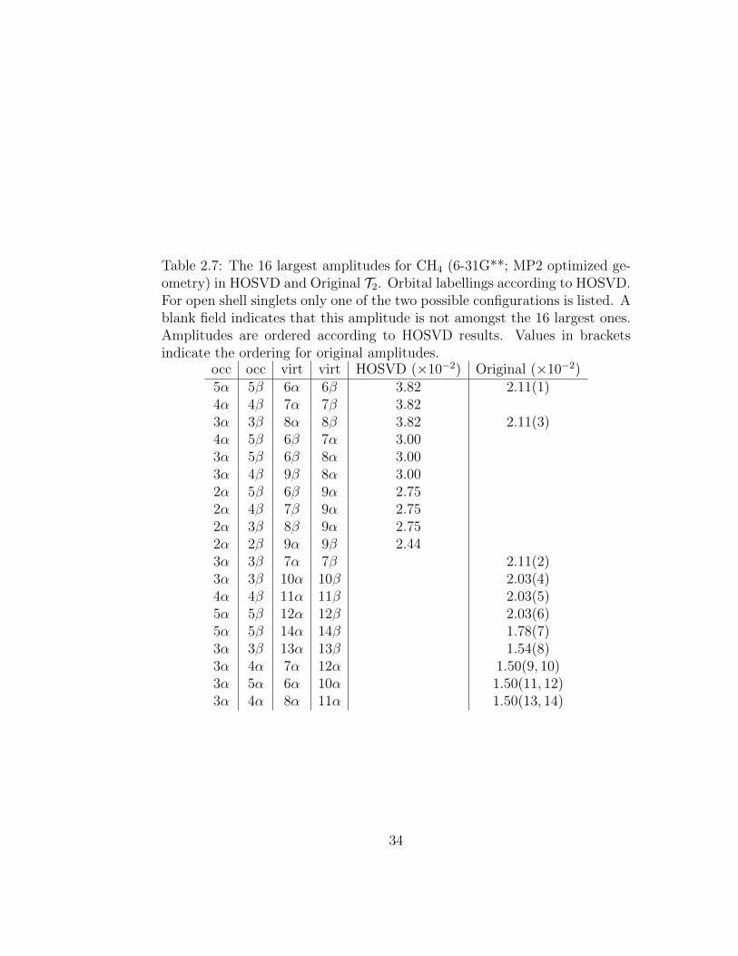
Table 2.7: The 16 largest amplitudes for CH4 (6-31G**; MP2 optimized ge-ometry) in HOSVD and Original T2. Orbital labellings according to HOSVD.For open shell singlets only one of the two possible configurations is listed. Ablank field indicates that this amplitude is not amongst the 16 largest ones.Amplitudes are ordered according to HOSVD results. Values in bracketsindicate the ordering for original amplitudes.
occ occ virt virt HOSVD (×10−2) Original (×10−2)5α 5β 6α 6β 3.82 2.11(1)4α 4β 7α 7β 3.823α 3β 8α 8β 3.82 2.11(3)4α 5β 6β 7α 3.003α 5β 6β 8α 3.003α 4β 9β 8α 3.002α 5β 6β 9α 2.752α 4β 7β 9α 2.752α 3β 8β 9α 2.752α 2β 9α 9β 2.443α 3β 7α 7β 2.11(2)3α 3β 10α 10β 2.03(4)4α 4β 11α 11β 2.03(5)5α 5β 12α 12β 2.03(6)5α 5β 14α 14β 1.78(7)3α 3β 13α 13β 1.54(8)3α 4α 7α 12α 1.50(9, 10)3α 5α 6α 10α 1.50(11, 12)3α 4α 8α 11α 1.50(13, 14)
34
40
50
60
70
80
90
100
% M
P2
Co
rr E
H4, R2=1.2A
6-31G 6-31G** 6-31++G**
1 2
4
0
10
20
30
0 2 4 6 8 10 12 14 16 18 20 22
number of virtuals included
34
5 7
cutoff: 0.1
Figure 2.6: recovery of % MP2 correlation energy vs. number of virtualorbitals included for linear H4 (R1 = 0.76A, R2 = 1.2 A) in various basissets. Box: the eight most correlating virtual orbitals.
lack the symmetric arrangement observed for HOSVD (Tables 2.5 to 2.7).
Table 2.8 shows the percentage MP2 correlation energy that is recoveredfor H2 in a (1, 1) active space and two H2 molecules at large distance (R= 5.0 A) in a (2,2) active space. The data suggests that HOSVD preservessize-extensivity properties.
2.3.2 Connection between HOSVD T2 and MP2 Natu-ral Orbitals
We are interested to cast the HOSVD in the language of quantum chemistry,specifically in the case of the T2 amplitudes. In doing so, it is crucial torecall that the HOSVD consists of d SVDs, which can be formulated as d
35
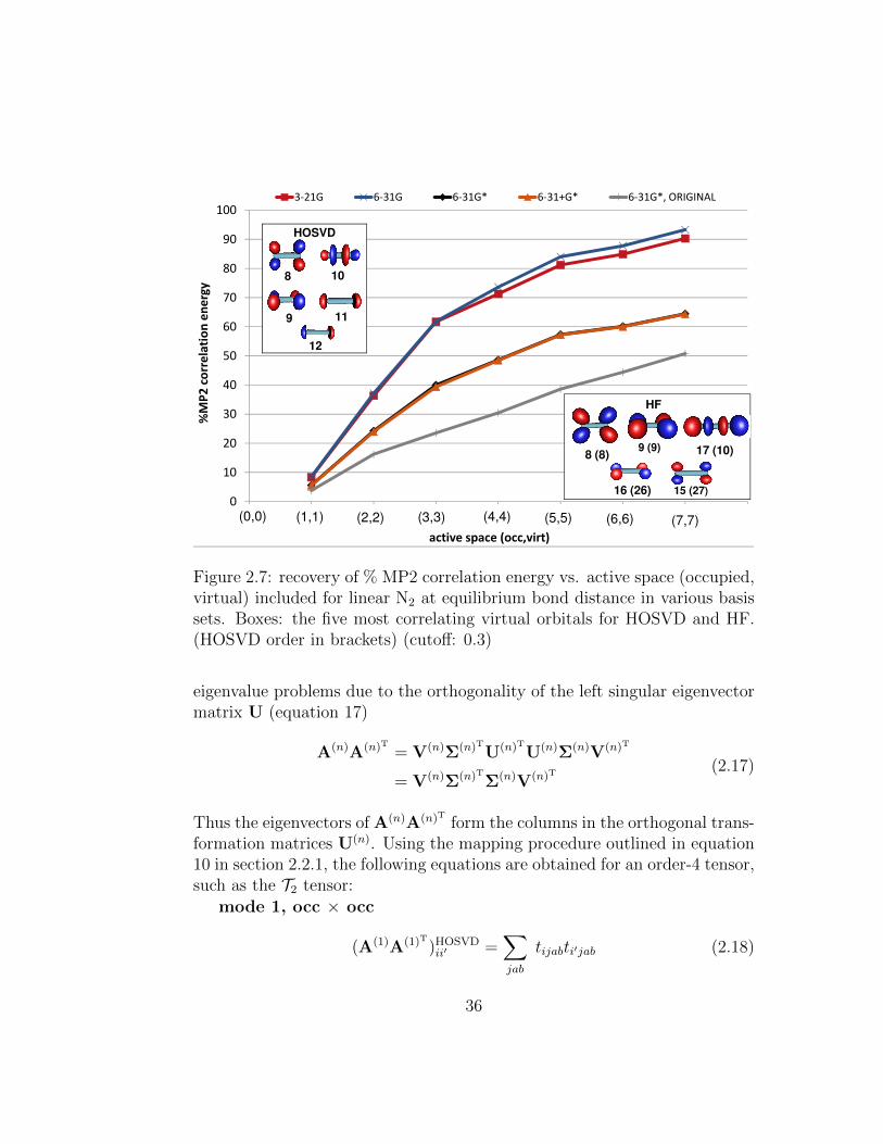
40
50
60
70
80
90
100%
MP
2 c
orr
ela
tio
n e
ne
rgy
3-21G 6-31G 6-31G* 6-31+G* 6-31G*, ORIGINAL
8
9
10
11
12
HOSVD
0
10
20
30
0 1 2 3 4 5 6 7 8
%M
P2
co
rre
lati
on
en
erg
y
active space (occ,virt)
(0,0) (1,1) (2,2) (3,3) (4,4) (5,5) (6,6) (7,7)
17 (10)8 (8)
16 (26)
9 (9)
15 (27)
HF
Figure 2.7: recovery of % MP2 correlation energy vs. active space (occupied,virtual) included for linear N2 at equilibrium bond distance in various basissets. Boxes: the five most correlating virtual orbitals for HOSVD and HF.(HOSVD order in brackets) (cutoff: 0.3)
eigenvalue problems due to the orthogonality of the left singular eigenvectormatrix U (equation 17)
A(n)A(n)T = V(n)Σ(n)TU(n)TU(n)Σ(n)V(n)T
= V(n)Σ(n)TΣ(n)V(n)T(2.17)
Thus the eigenvectors of A(n)A(n)T form the columns in the orthogonal trans-formation matrices U(n). Using the mapping procedure outlined in equation10 in section 2.2.1, the following equations are obtained for an order-4 tensor,such as the T2 tensor:
mode 1, occ × occ
(A(1)A(1)T)HOSVDii′ =
∑jab
tijabti′jab (2.18)
36

40
60
80
100
% M
P2
Co
rr E
N2, opt geom
6-31G*
6-31G
3-21G
0
20
0 5 10 15 20 25
# virtual orbitals included
Figure 2.8: recovery of % MP2 correlation energy vs. number of virtualorbitals included for N2 at equilibrium bond distance in various basis sets.
Table 2.8: %MP2 energy for H2 [(1, 1) active space] and two H2 molecules atlarge distance (R = 5.0 A), [(2, 2) active space]
Molecule 6-31G 6-31G** 6-31++GH2 73.0 45.1 45.0H4 73.0 45.1 45.0
37
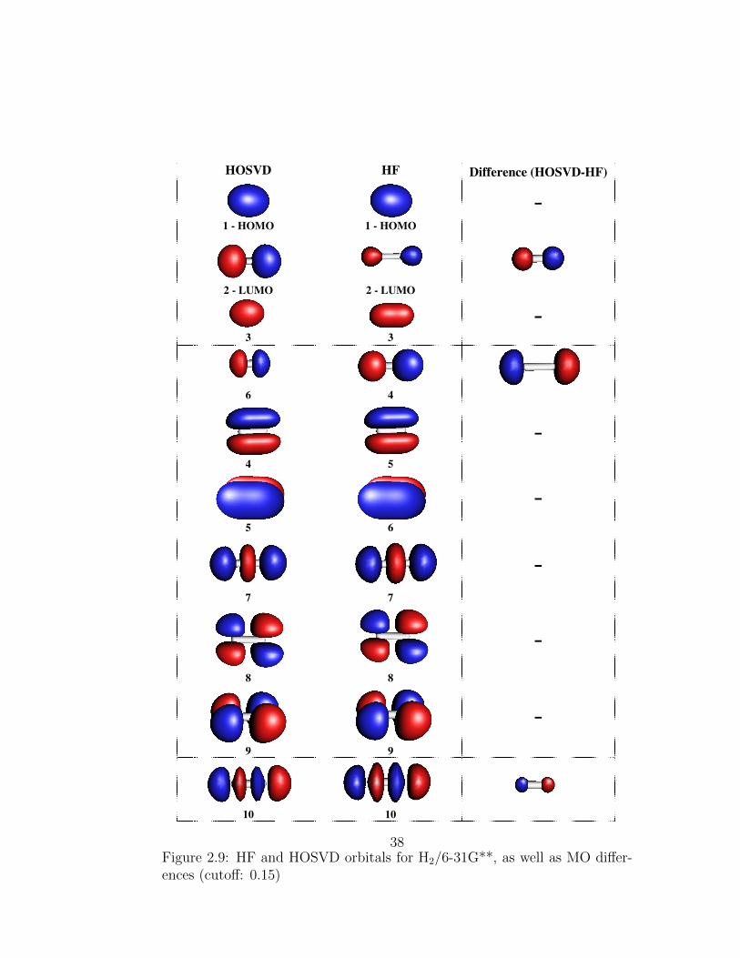
HOSVD HF Difference (HOSVD-HF)
-
1 - HOMO 1 - HOMO
2 - LUMO 2 - LUMO
-
3 3
6 4
-
4 5
-
5 6
-
7 7
-
8 8
-
9 9
10 10
Figure 2.9: HF and HOSVD orbitals for H2/6-31G**, as well as MO differ-ences (cutoff: 0.15)
38
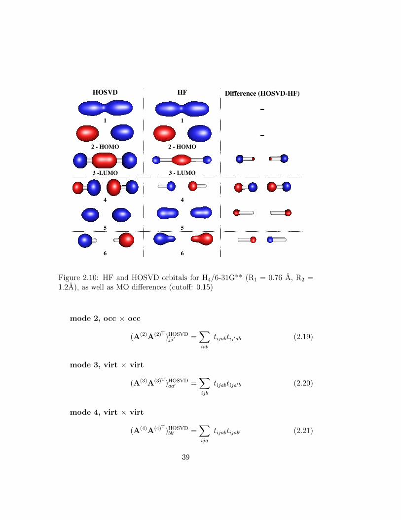
HOSVD HF Difference (HOSVD-HF)
-
1 1
-
2 - HOMO 2 - HOMO
3 -LUMO 3 - LUMO
4 4
5 5
6 6
Figure 2.10: HF and HOSVD orbitals for H4/6-31G** (R1 = 0.76 A, R2 =1.2A), as well as MO differences (cutoff: 0.15)
mode 2, occ × occ
(A(2)A(2)T)HOSVDjj′ =
∑iab
tijabtij′ab (2.19)
mode 3, virt × virt
(A(3)A(3)T)HOSVDaa′ =
∑ijb
tijabtija′b (2.20)
mode 4, virt × virt
(A(4)A(4)T)HOSVDbb′ =
∑ija
tijabtijab′ (2.21)
39
Comparing the above expressions with the equation for the one-particleunrelaxed MP2 density, D21
pq [258]:
(D)21qp =
∑aij
tapij taqij −
∑iab
tabiq tabip (2.22)
reveals the following relationship:
(D)21pq = (A(4)A(4)T)HOSVD
ll′ − (A(1)A(1)T)HOSVDjj′ (2.23)
This shows that the HOSVD T2 orbitals are identical to the unrelaxedMP2 natural orbitals, since they involve the trace of the left and right handside of equation 23, which are equivalent.
2.3.3 Higher Order Orthogonal Iterations (HOOI) vs.HOSVD
It has been shown that a simple truncation of the core tensor obtained from aHOSVD yields sub-optimal results measured in the norm of the difference [2].However, it is found to be a good starting point for an iterative alternatingleast squares (ALS) algorithm, such as the Higher-order Orthogonal Iteration(HOOI) proposed by De Lathauwer et al. [2]. This algorithm is based on thedominant singular vectors of A(n) and the SVD (see Fig. 2.14), and is an effi-cient alternative to the previously developed method by Kapteyn, Neudecker,and Wansbeek [230]. Our preliminary calculations indicate that HOOI doesnot significantly improve the results obtained from HOSVD. Typically theimprovement is less than a 2 percent increase in correlation energy comparedto HOSVD, for model systems studied in section 3. This is in accordancewith previous numerical observations [2]. The exception is CH4, which yieldsimprovements of more than 5 percent in small active spaces.
2.4 Conclusion
HOSVD yields active spaces that coincide with physical intuition. Therefore,orbitals obtained from a decomposed T2 MP2 tensor may be useful as aninitial guess for higher level CC or MBPT calculations.
40
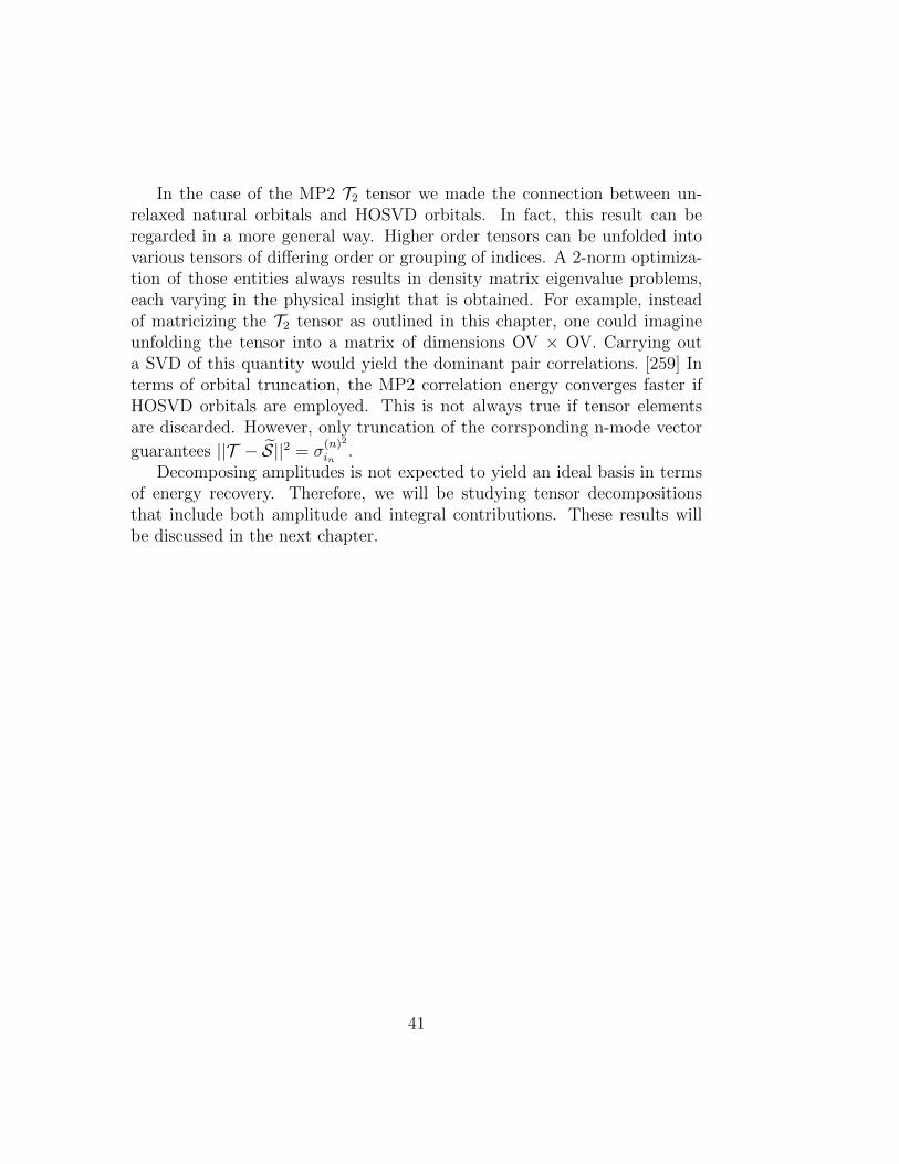
In the case of the MP2 T2 tensor we made the connection between un-relaxed natural orbitals and HOSVD orbitals. In fact, this result can beregarded in a more general way. Higher order tensors can be unfolded intovarious tensors of differing order or grouping of indices. A 2-norm optimiza-tion of those entities always results in density matrix eigenvalue problems,each varying in the physical insight that is obtained. For example, insteadof matricizing the T2 tensor as outlined in this chapter, one could imagineunfolding the tensor into a matrix of dimensions OV × OV. Carrying outa SVD of this quantity would yield the dominant pair correlations. [259] Interms of orbital truncation, the MP2 correlation energy converges faster ifHOSVD orbitals are employed. This is not always true if tensor elementsare discarded. However, only truncation of the corrsponding n-mode vector
guarantees ||T − S||2 = σ(n)2
in.
Decomposing amplitudes is not expected to yield an ideal basis in termsof energy recovery. Therefore, we will be studying tensor decompositionsthat include both amplitude and integral contributions. These results willbe discussed in the next chapter.
41

HOSVD HF Difference (HOSVD-HF)
-
1 1
-
2 2
3 3
-
4 4
5 5
-
6 -HOMO 7 -HOMO
-
7 -HOMO 6 -HOMO
Figure 2.11: HF and HOSVD occupied orbitals for N2/6-31G* (at equilib-rium), as well as MO differences (cutoff: 0.15)
42
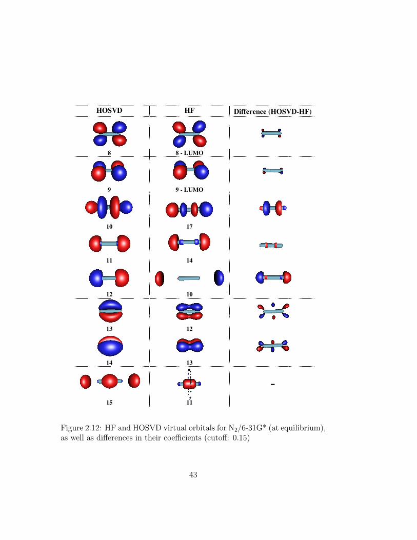
HOSVD HF Difference (HOSVD-HF)
8 8 - LUMO
9 9 - LUMO
10 17
11 14
12 10
13 12
14 13
-
15 11
Figure 2.12: HF and HOSVD virtual orbitals for N2/6-31G* (at equilibrium),as well as differences in their coefficients (cutoff: 0.15)
43

Occupied Virtual
2 9
3, 4, 5 6, 7, 8
Figure 2.13: HOSVD occupied-virtual correlating orbital pairs for CH4 (cut-off: 0.2) (6-31G**; MP2 optimized geometry)
procedure HOOI(T , R1, R2, ..., Rd)
initialize U(n) ∈ RIn×Rn for n = 1, ..., d using HOSVDrepeat
for n = 1, ..., N do
W ← T ×1 U(1)T × ...×n−1 U(n−1)T ×n+1 U(n+1)T × ...×d U(d)T
U(n) ← Rn leading left singular vectors of W(n)
end foruntil convergence criterion met or maximum iterations reached
S ← T ×1 U(1)T ×2 U(2)T × ..×d U(d)T
return S, U(1), U(2), ..., U(d)
end procedure
Figure 2.14: Adapted from [1]. Alternating least squares algorithm to computea rank-(R1, R2, ..., Rd) Tucker decomposition for a tensor, T ∈ RI1×I2×...×Id .Also known as the higher-order orthogonal iteration (HOOI).
44

Chapter 3
Beyond Natural Orbitals:Higher Order Singular ValueDecomposition ofEnergy-Weighted Integrals
In the search for the transformation which results in the maximal recoveryof correlation energy as a function of orbital truncation, numerical studiesreveal that non-unitary transformations can considerably outperform natu-ral orbitals or orbital-optimization methods. In particular, we show that onepossible transformation can be constructed by the higher order singular valuedecomposition (HOSVD) of energy-weighted integrals. Test calculations onthe HOSVD of energy-weighted integrals of second order Møller Plesset Per-turbation (MP2) yield considerably faster convergence of correlation energycompared to unrelaxed (frozen) natural orbitals and those obtained fromorbital-optimizations for small- and medium-sized active spaces. Further-more, we show that the energy-weighted transformation obtained for MP2 istransferable to Coupled-cluster (CC) methods.
3.1 Introduction
In quantum chemistry higher order tensors arise naturally, for example in thewave-function based description of electron correlation [221]. The so-called
45

“curse of dimensionality” [222] (exponential growth of elements in an arraywith number of indices) restricts highly accurate calculations to very smallsystems. In order to address this problem, active space methods [51, 77], lo-cal correlation approaches [115,260,261] or a combination of both [262] havebeen of great interest to the community for many decades. Other approachesrelated to the compression and truncation of the virtual space are frozen nat-ural orbitals (FNOs) [138–141,146,263–266], optimized virtual orbital spaces(OVOS) [147,148,267] or pair natural orbitals (PNOs) [143,144,268–270].
Another way to approach the dimensionality problem is to obtain low-parametric representations via tensor decompositions. These have alreadybeen successfully applied in numerous other fields, such as signal process-ing [202–204], graph analysis [205–207], neuroscience [213–216] and computervision [217–220], and have lately also become of interest in quantum chem-istry [271–274].
Recently, we have made connections between various different tensor de-composition methods and existing approaches in quantum chemistry [271].For example, the CANDECOMP/PARAFAC method [234, 236–238], whichdecomposes a multilinear array into a sum of Kronecker products of rank-onetensors, is equivalent to a (truncated) configuration interaction (CI) expan-sion [275]. On the other hand, the higher order singular value decomposition(HOSVD) [257] can be related to orbital active space methods, such as thecomplete active space self-consistent field (CASSCF) [51] approach. In par-ticular, we have proven that in the case of MP2 T2 amplitudes the HOSVDand unrelaxed (frozen) natural orbitals are equivalent [271].
However, as noted in the previous chapter, a decomposition of the am-plitudes and therefore frozen natural orbitals are expected to be sub-optimalwith respect to correlation energy recovery, as the MP2 energy expressiondoes not only incorporate amplitudes, tijab, but also integrals, Iijab = 〈φiφj||φaφb〉:
EMP2 = −1
4
∑ijab
tijabIijab (3.1)
This motivated a study of various energy weighted decomposition ap-proaches, which will be the subject of this chapter.
46
The chapter is structured as follows: In the first part the basic principlesof the HOSVD are reviewed. We then proceed to justify, derive and testthe energy-weighted HOSVD in the context of MP2 in sections III (Theory)and IV (Numerical Results). Finally it is shown that the improved coordi-nate transformation for MP2 is transferable to coupled-cluster techniques insection 3.5.
3.2 Notation and Basic Definitions
The following notation will be used throughout the chapter: scalars are in-dicated by lower- or upper-case letters (a, b, ...;A,B, ...) (italic), matrices arewritten in bold-face capitals (A,B, ...), and tensors are indicated as calli-graphic capitals (A,B,...).A tensor with d indices will be referred to as a d-mode tensor or an order-dtensor.The Frobenius norm of a tensor A, ||A||F is defined as
||A||Fdef=√〈A,A〉 (3.2)
The n-mode product A ×n U of a tensor A ∈ RI1×I2×...×Id with a matrixU ∈ RJn×In is an (I1×I2× ...×In−1×Jn×In+1× ...×Id) tensor with entries:
(A×n U)i1i2...in−1jnin+1...iddef=∑in
ai1i2...in−1inin+1...idujnin (3.3)
Other definitions specific to this chapter will be given at the appropriatepoint.
3.3 Theory
3.3.1 Overview of the HOSVD
The well-known singular value decomposition of a rectangular matrix A ∈RI1×I2 in two dimensions takes the following form [276]:
aij =∑i′j′
σi′j′uii′vj′j (3.4)
47
where the matrix Σ ∈ RI1×I2 is diagonal and holds the singular values indecreasing magnitude and U ∈ RI1×I2 and V ∈ RI2×I2 are unitary transfor-mation matrices that contain the left and right singular vectors, respectively.The unitary matrices each only act on one of the dimensions. In order toemphasize this, the above expression can be re-written as:
aij =∑i′j′
σi′j′u(1)i′i u
(2)j′j (3.5)
where the superscripts indicate the corresponding mode the matrix trans-forms.
Generalization of the above expression to a mode-d tensor, yields:
tij...d =∑i′j′...d′
si′j′...d′u(1)i′i u
(2)j′j ...u
(d)d′d (3.6)
The tensor S in the above expression is referred to as the core tensor. In themulti-dimensional case (d > 2) S is not necessarily diagonal. This impliesthat rank truncation based on its singular values may be sub-optimal, aswill be discussed in more detail below. The transformation matrices U(n)
are known as mode factors and are constrained to be unitary in the HOSVDformulation [257]. This allows the core tensor to be found via
si′j′...d′ =∑ij...d
tij...d(u(1)i′i )T (u
(2)j′j)
T ...(u(d)d′d)
T (3.7)
Rank truncation of the core tensor, S, which is obtained by keeping onlythe largest n-mode singular vectors is expected to introduce smaller errors asmeasured with regards to the untruncated result than the tensor in the orig-inal basis, T . If the tensor under consideration is composed of MP2 ampli-tudes, the unitary transformation matrices correspond to occupied-occupiedand virtual-virtual rotations. Therefore rank-truncation will correspond toorbital truncations in the occupied and virtual spaces, respectively. As wasshown in the previous chapter [271], orbitals obtained from the HOSVD ofMP2 amplitudes are equivalent to unrelaxed natural orbitals and convergemuch more rapidly than canonical orbitals. However, as mentioned in theintroduction, orbitals obtained from such a decomposition are expected toyield a sub-optimal convergence of correlation energy.
48
3.3.2 HOOI vs. Orbital Optimization for MP2
On the quest for the fastest converging orbitals, we were interested if we couldfind a connection between a form of HOSVD and methods involving orbitaloptimization. If this holds true, then only the decomposition of coordinatetransformed tensors can yield faster convergence.
Orbital-optimization requires the Lagrangian to be minimized with re-spect to orbital rotations, Θ. Typically, natural orbitals are found to be agood guess for such methods. Since we have shown that the orbitals ob-tained from the higher-order singular value decomposition of the MP2 T2
amplitudes are equivalent to the unrelaxed natural orbitals [271], it may bepossible that an iterative technique involving the decomposition of the T2
amplitudes yields similar results to orbital optimization.
As mentioned in the previous section, rank reduction obtained from HOSVDfor a core tensor of order greater than 2 is not necessarily optimal [2]. Given areal N -th order tensor T ∈ RI1×I2×...×IN , finding its best rank-R1, R2, ..., RN
(Rn ∈ N; 1 ≤ Rn ≤ In) approximation, T , requires the minimization of theleast-squares cost function [2]
min f(T ) = ||T − T ||2F (3.8)
It can be shown, that minimizing the above cost function is equivalent tomaximizing the function g over the unitary transformation matrices U(1) ∈RI1×R1 ,U(2) ∈ RI2×R2 , ...,U(N) ∈ RIN×RN
max g(U(1),U(2), ...,U(N)) =
= ||T ×1 U(1)T ×2 U(2)T ...×N U(N)T ||2F =
= ||T ||2F
(3.9)
The above cost function g yields an alternating least squares algorithm(ALS), called the higher order orthogonal iterations (HOOI) [2]. A pseudo-algorithm for the HOOI is given in Figure 3.3. A step in the HOOI loopconsists of optimizing the estimate of one of the matrices U(1),U(2), ...,U(N)
using the HOSVD procedure, while the other matrices are kept constant.
In order to compare to the HOOI decomposition of T2 amplitudes from
49
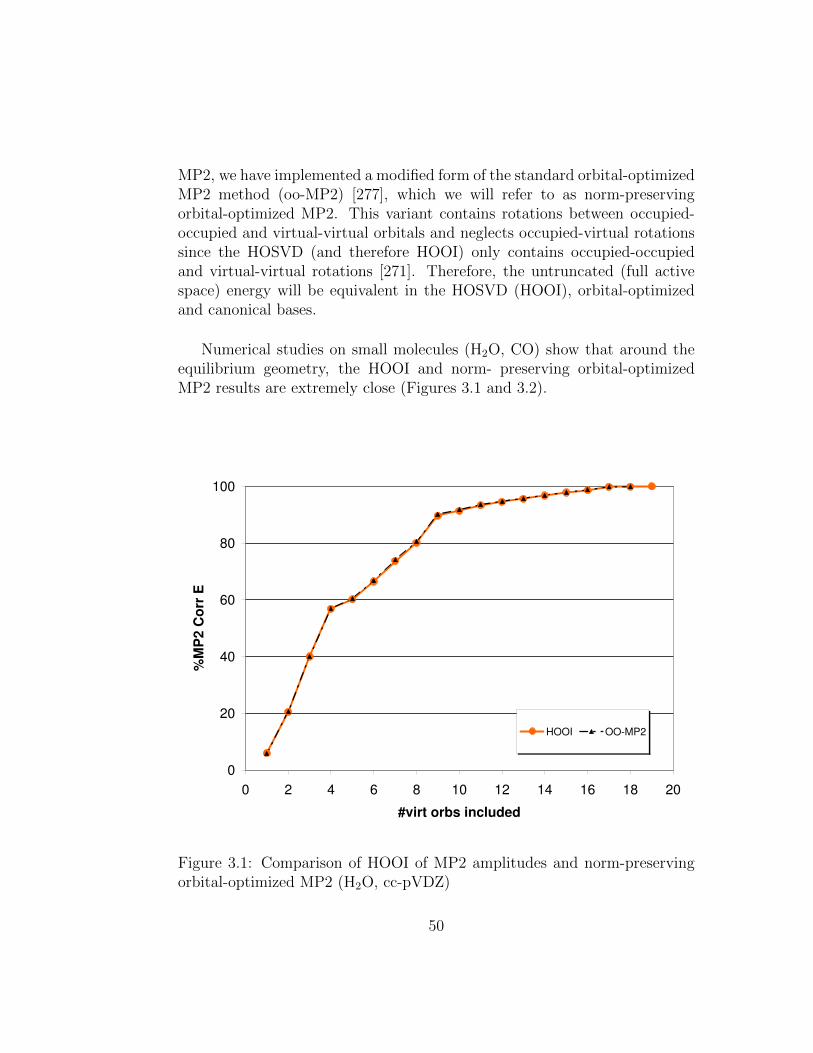
MP2, we have implemented a modified form of the standard orbital-optimizedMP2 method (oo-MP2) [277], which we will refer to as norm-preservingorbital-optimized MP2. This variant contains rotations between occupied-occupied and virtual-virtual orbitals and neglects occupied-virtual rotationssince the HOSVD (and therefore HOOI) only contains occupied-occupiedand virtual-virtual rotations [271]. Therefore, the untruncated (full activespace) energy will be equivalent in the HOSVD (HOOI), orbital-optimizedand canonical bases.
Numerical studies on small molecules (H2O, CO) show that around theequilibrium geometry, the HOOI and norm- preserving orbital-optimizedMP2 results are extremely close (Figures 3.1 and 3.2).
0
20
40
60
80
100
0 2 4 6 8 10 12 14 16 18 20
#virt orbs included
%M
P2
Co
rr E
HOOI OO-MP2
Figure 3.1: Comparison of HOOI of MP2 amplitudes and norm-preservingorbital-optimized MP2 (H2O, cc-pVDZ)
50
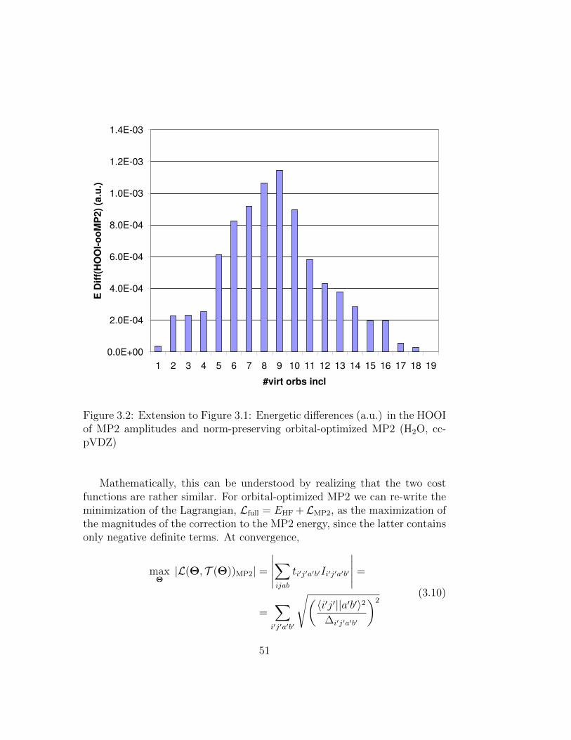
0.0E+00
2.0E-04
4.0E-04
6.0E-04
8.0E-04
1.0E-03
1.2E-03
1.4E-03
1 2 3 4 5 6 7 8 9 10 11 12 13 14 15 16 17 18 19
#virt orbs incl
E D
iff(
HO
OI-
oo
MP
2)
(a.u
.)
Figure 3.2: Extension to Figure 3.1: Energetic differences (a.u.) in the HOOIof MP2 amplitudes and norm-preserving orbital-optimized MP2 (H2O, cc-pVDZ)
Mathematically, this can be understood by realizing that the two costfunctions are rather similar. For orbital-optimized MP2 we can re-write theminimization of the Lagrangian, Lfull = EHF +LMP2, as the maximization ofthe magnitudes of the correction to the MP2 energy, since the latter containsonly negative definite terms. At convergence,
maxΘ|L(Θ, T (Θ))MP2| =
∣∣∣∣∣∑ijab
ti′j′a′b′Ii′j′a′b′
∣∣∣∣∣ =
=∑i′j′a′b′
√(〈i′j′||a′b′〉2
∆i′j′a′b′
)2(3.10)
51
where ∆ijab = faa + fbb − (fii + fjj).
Recall from equation (10) that the HOOI of T will involve the cost func-tion
max g(U(1),U(2),U(3),U(4)) = max||T ||2F
= max∑ijab
(〈i′j′||a′b′〉)2
(∆i′j′a′b′)2
(3.11)
From this analysis we expect the HOOI of T to deviate most from unre-laxed oo-MP2 around the dissociation limit, where ∆ijab → 0.
Since the HOOI of the MP2 T2 amplitudes yields numerically similarresults to norm-preserving orbital-optimized MP2, we can conclude that toobtain improved results, we must explore non-unitary transformations.
3.3.3 Proposed Coordinate Transformation for MP2
As shown in the previous section, the only way to improve considerably be-yond natural orbitals or orbitals resulting from methods involving orbitaloptimization is by non-unitary, i.e. coordinate transformations. Here weagain investigate the simplest case, namely MP2.
We start from the Hylleraas functional
L(T ) =1
4Tr(T · A · T + 2T · I) (3.12)
where
aijab,klcd =(facδbd + fbdδac)δikδjl−(fikδjl + fjlδik)δacδbd
(3.13)
and tijab and Iijab are as defined previously.
Next we insert the resolution of identity into equation (3.12)
L(T ) =1
4Tr(T †1†A1T + 2T †1I) (3.14)
52

procedure HOOI(T , R1, R2, ...Rd)Guess:
for n = 1, ..., d doU(n) ← Rn leading left singular vectors of A(n)
end forwhile ||Bk||F − ||Bk+1||F > threshold
P(1)k+1 = T ×2 U
(2)T
k ×3 U(3)T
k ...×d U(d)T
k
U(1)k+1 ← R1 leading left singular vectors of P
(1)k+1
P(2)k+1 = T ×1 U
(1)T
k+1 ×3 U(3)T
k ...×d U(d)T
k
U(2)k+1 ← R2 leading left singular vectors of P
(2)k+1
...
P(d)k+1 = T ×1 U
(1)T
k+1 ×2 U(2)T
k+1 ...×d−1 U(d−1)T
k+1
U(d)k+1 ← Rd leading left singular vectors of P
(d)k+1
k = k + 1end while
B ← T ×1 U(1)T
max ×2 U(3)T
max ...×d U(d)T
max
return B,U(1)max,U
(2)max, ...,U
(d)max
end procedure
Figure 3.3: HOOI procedure. Adapted from [2].
53
which yields
L(T ) =1
4Tr[(X−1T )†(X †AY)(Y−1T ) + 2(Y−1T )†(Y†I)] (3.15)
where we used X−1X = 1 and Y−1Y = 1.
This can be re-written as
L(T ) =1
4Tr[T † ˘AT + 2T †I
](3.16)
where breve ( ˘ ) and tilde ( ˜ ) indicate which transformation (X or Y) wasapplied.
Now we ask the question how to achieve faster convergence by reducingthe degrees of freedom. In particular this corresponds to finding the condi-
tions for which ˘A becomes diagonal
˘A = X †AY = 1 (3.17)
LetX † = Am (3.18)
which implies thatY = A−(m+1) (3.19)
Next we insert these definitions into the above equation for the Lagrangian,yields:
L(T ) =1
4Tr
[{(A−m
)† T }†{Am+1T}
+2
{Am+1T
}† {(A−(m+1)
)† I}] (3.20)
which can be re-written in our more compact notation as:
L(T ) =1
4Tr[T †T + 2T †I
](3.21)
54
Solving for the amplitude equations requires:
dL(T )
dT= 0 (3.22)
Thus:
dL(T )
dT=
1
4Tr[(A−m
) (Am+1T
)+(Am+1
)† ((A−m)† T )+2(Am+1
)† (A−(m+1)I)]
= 0(3.23)
which can be re-written as:
(A−m)T +(Am+1
)† T = −2(Am+1
)† I (3.24)
Solving for T yields:
T = −[2I +
(A−(m+1)
)† (A−m) T ] (3.25)
Thus the Lagrangian can now be re-written as:
L(T ) =1
4Tr[{−2I† − T †
(A−m
)† (A−(m+1))}T + 2T †I
](3.26)
As a result of the symmetry properties of the integrals, amplitudes andtensor A (which requires assuming a real-valued Fock matrix) the aboveexpression simplifies to:
L(T ) =1
4Tr[T(A−(2m+1)
)T]
(3.27)
We are seeking a transformed tensor, T , to decompose via HOSVD, andthen truncate the resulting core tensor, aiming to obtain faster convergencethan before. Such a goal is likely to be best achieved by decomposing T afterchoosing m so that the explicit dependence on A is removed. This is the caseif:
m = −1
2(3.28)
55

This yieldsI = A−1/2I (3.29)
andT = −2I (3.30)
This is a dilatory transformation into energy-weighted 4-index coordinates.Since the tensor A contains Fock elements we will refer to this as an energy-weighted decomposition.
In the canonical basis,
aijab,klcd = ∆ijab = faa + fbb − (fii + fjj) (3.31)
and the quantity to be decomposed becomes
(wijab)1/2 = (tijabIijab)
−1/2 (3.32)
And the energy expression takes the form
EMP2 = −1
4
∑ijab
(wijab)1/2 (wijab)
1/2 (3.33)
The result that a tensor of the form of W1/2 should be chosen is notsurprising if the expression for the energy is considered in equation (7.2).Decomposition of T yields the optimal transformation matrices for T , butdoes not consider the optimal transformations for the integrals. Decom-position of W1/2, on the other hand, will involve both the amplitudes andintegrals in the determination of the optimal transformation.
Another property of the energy-weighted decomposition worth mention-ing is that the elements in W1/2 are positive-semidefinite. This yields trun-cated correlation energies that always will be an upper bound to the full MP2energy. This is, however, not guaranteed for the decomposition of MP2 am-plitudes (or integrals). In this case positive contributions to the correlationenergy can result and thus the recovery of correlation energy can be greaterthan 100 percent for truncated orbital spaces.
Interestingly, connections to amplitude and integral decompositions can
56
be made, if other limiting cases of equation (3.27) are considered
Case 1: Let m = −1, then
L(T ) =1
4T AT (3.34)
andT = T (3.35)
this corresponds to the decomposition of the original T amplitudes.
L(T ) =1
4T (AT ) =
1
4T I (3.36)
Case 2: Let m = 0, then
L(T ) =1
4T A−1T (3.37)
andT = AT = I (3.38)
this corresponds to the decomposition of the original integrals.
3.4 Numerical Results
In the previous section we have shown that a faster convergence in correlationenergy for the case of MP2 should be obtained by decomposing the quantityW1/2, which in a canonical basis takes the form:
(wijab)1/2 = (tijabIijab)
−1/2 (3.39)
Numerical studies on various small molecules in different basis sets have beencarried out to verify this conclusion. As can be seen from Figures 3.4 to 3.7decomposition ofW1/2 (depicted as triangles) yields considerably faster con-vergence in correlation energy compared to unrelaxed natural orbitals (Tdecomposition) and norm-conserving orbital-optimized MP2 (oo-MP2) if asmall to medium number of virtual orbitals are included. Particularly inter-esting are the effects obtained for the pairing and full valence active spaces,which are the most commonly chosen in calculations. In the case of CH4
57
(cc-pVDZ) (Figure 3.4) the pairing and full valence space involves four vir-tual orbitals. At this point, canonical orbitals only recover 14% of the MP2correlation energy. A major improvement is obtained by using unrelaxed nat-ural orbitals (which is equivalent to decomposing the T2 amplitudes), whichyields 36% of the MP2 correlation energy. If W1/2 is decomposed, however,more than 62% of the correlation energy is recovered. The results obtainedfor H2O (cc-pVDZ, Figure 3.5) are equally remarkable. Here the full valenceand pairing active spaces correspond to the (8,6) and (8,8) space, respec-tively. Interestingly, we do not observe any change in slope at the pairingactive space, indicating that this does not seem to be a natural choice forthis molecule. Nevertheless, an improvement in correlation energy recoveryis observed for the W1/2 decomposition (35%) compared to canonical (11%)and unrelaxed natural orbitals (20%). For the (8,8) active space 22%, 55%and 68% of the MP2 correlation energy are recovered for the canonical, un-relaxed natural orbitals and W1/2 decomposed cases, respectively. Althoughthe decomposition of the T2 amplitudes suggests a natural closing at the(8,8) active space, the W1/2 decomposition indicates an (8,7) active space.In order to understand the effect of basis set, we also carried out calcula-tions on H2O at the cc-pVTZ level (Figure 3.6). Unrelaxed natural orbitalsyield 15% and 44% correlation energy recovery for the (8,6) and (8,8) activespaces, respectively, whereas decomposition of W1/2 recovers 30% and 61%.Again, while decomposition of the T2 amplitudes suggests that an (8,8) activespace should be chosen, theW1/2 decomposition favors an (8,7) active space.Finally, in the case of CO (Figure 3.7) the full valence (10,8) active spaceseems to be the more natural choice than the pairing active space, (10,10).TheW1/2 decomposition again provides a considerably faster convergence incorrelation energy (61% and 71%) for the (10,8) and (10,10) active spacescompared to the unrelaxed natural orbitals (43% and 56%).
For the active spaces discussed above, the energy-weighted form of MP2yields the fastest convergence in correlation energy known to date. When alarge fraction of virtual orbitals are retained, a cross-over with the decom-position of T2 is observed for H2O (cc-pVTZ, Figure 3.6) and CO (cc-pVDZ,Figure 3.7). This arises because the tensor to be decomposed is multidimen-sional, and would not be expected if a decomposed matrix was truncated. Itwas proven that for the order-2 case an optimality property condition holds,which states that the singular value decomposition yields the closest rankR approximation of a matrix. However, due to the higher-order nature of
58
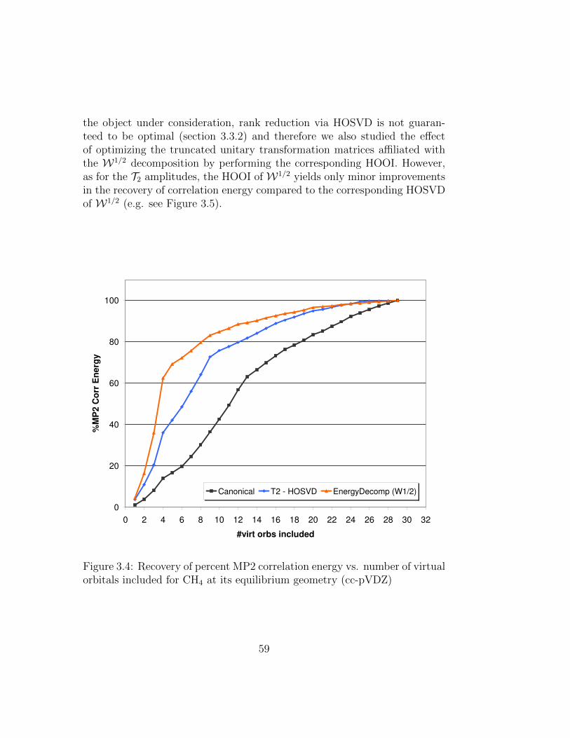
the object under consideration, rank reduction via HOSVD is not guaran-teed to be optimal (section 3.3.2) and therefore we also studied the effectof optimizing the truncated unitary transformation matrices affiliated withthe W1/2 decomposition by performing the corresponding HOOI. However,as for the T2 amplitudes, the HOOI of W1/2 yields only minor improvementsin the recovery of correlation energy compared to the corresponding HOSVDof W1/2 (e.g. see Figure 3.5).
0
20
40
60
80
100
0 2 4 6 8 10 12 14 16 18 20 22 24 26 28 30 32
#virt orbs included
%M
P2 C
orr
En
erg
y
Canonical T2 - HOSVD EnergyDecomp (W1/2)
Figure 3.4: Recovery of percent MP2 correlation energy vs. number of virtualorbitals included for CH4 at its equilibrium geometry (cc-pVDZ)
59

Figure 3.5: Recovery of percent MP2 correlation energy vs. number of virtualorbitals included for H2O at its equilibrium geometry (cc-pVDZ)
3.5 Transferability to Coupled-Cluster Meth-
ods
Finally, we were interested if the energy-weighted MP2 quantities from sec-tion III could be used in coupled-cluster (CC) calculations. As the objectsobtained from the dilatory transformation do not correspond to orbitals, thecorresponding coupled-cluster equations would have to be modified accord-ingly.
For simplicity we choose to use the linearized coupled-cluster doubles(LCCD) equations as a case study. However, the results shown below aregenerally applicable to any form of coupled-cluster theory.
60

Figure 3.6: Recovery of percent MP2 correlation energy vs. number of virtualorbitals included for H2O at its equilibrium geometry (cc-pVTZ). For clarityonly the first 20 of 53 virtual orbitals are shown.
The most general form of LCCD equations which are invariant to arbi-trary non-singular one-particle transformations:
E = E0 +1
4I ij..abt
ab..ij (3.40)
and
Iab..ij +1
2Iab..cdt
cd..ij +
1
2Ikl..ijt
ab..kl + A2[4Ibk..jct
ac..ik] =
F k.jtab..ik + F k
.i tab..ik + F b
.ctac..ij − F a
.ctcb..ij
(3.41)
61
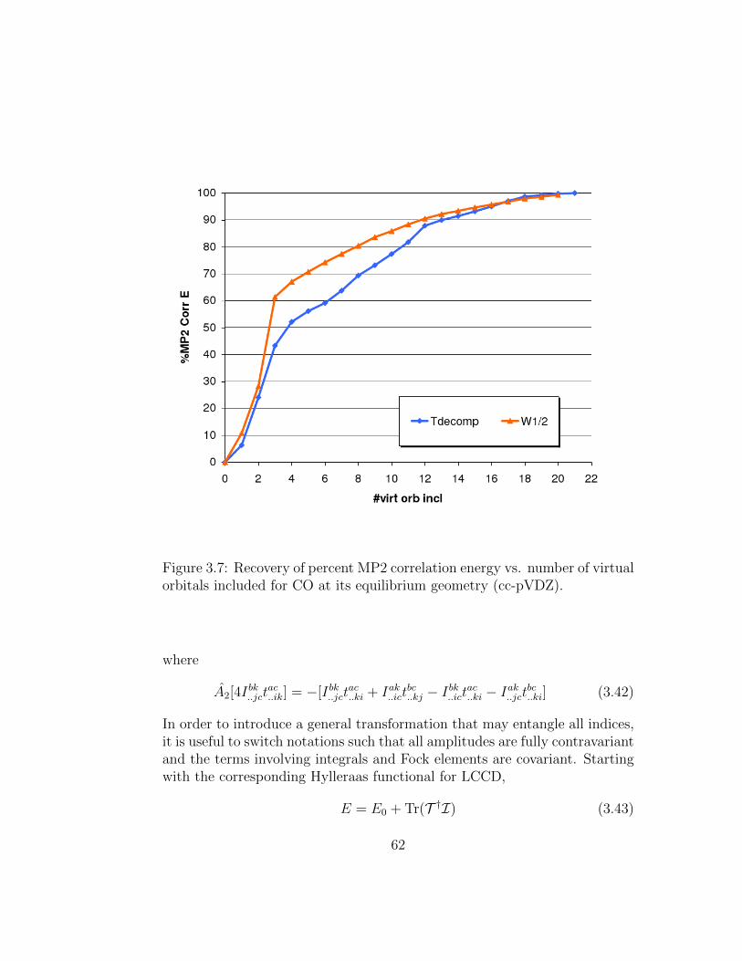
Figure 3.7: Recovery of percent MP2 correlation energy vs. number of virtualorbitals included for CO at its equilibrium geometry (cc-pVDZ).
where
A2[4Ibk..jctac..ik] = −[Ibk..jct
ac..ki + Iak..ict
bc..kj − Ibk..ictac..ki − Iak..jctbc..ki] (3.42)
In order to introduce a general transformation that may entangle all indices,it is useful to switch notations such that all amplitudes are fully contravariantand the terms involving integrals and Fock elements are covariant. Startingwith the corresponding Hylleraas functional for LCCD,
E = E0 + Tr(T †I) (3.43)
62
whereI = AT +RT (3.44)
The explicit expressions for A and R are
Aijab;klcd = (facgik − gacfik)gbdgjl + gacgik(fbdgjl − gbdfjl) (3.45)
and
Rijab;klcd =− 1
2Iabcdgikgjl −
1
2Iklijgacgbd+
Ibljdgacgik − Ibkidgacgjl − Ialjcgbdgik + Iakidgbdgjl
(3.46)
This yields:
LLCCD = E0 + tijab[Aijab;klcd +Rijab;klcd]tklcd (3.47)
This allows us to treat LCCD analogously to MP2 (see equations (4.2) -(3.28) above)
LLCCD = E0 + Tr{T †X †[A+R]XT + 2T †(X †I)
}(3.48)
In the case of LCCD a transformation can be found, for which
X †[A+W ]X = 1 (3.49)
This will take the formX = (A+R)−1/2 (3.50)
and thusLLCCD = E0 + Tr
(T †T + 2T †I
)(3.51)
However, much more importantly, it is possible to use the transformationfound to be optimal for MP2
X ≡ A−1/2 (3.52)
From this it follows
LLCCD = E0 + Tr(T †[1 +A−1/2RA−1/2]T + 2T †I
)(3.53)
63

This shows that the transformations obtained from performing HOSVDon energy-weighted MP2 integrals are transferable to coupled-cluster calcu-lations.
3.6 Conclusions
We illustrate that in order to outperform unrelaxed natural orbitals or norm-preserving orbital-optimized MP2, coordinate transformations are necessary.In the case of MP2, a higher order singular value decomposition of energy-weighted integrals is derived starting from the Hylleraas functional. Numeri-cal results indicate that considerably faster convergence of correlation energyis obtained for small- and medium-sized active spaces compared to unrelaxednatural orbitals and orbital-optimized MP2. For these active space sizes, thehigher order singular value decomposition of energy-weighted integrals yieldsthe fastest converging MP2 correlation energy results to date. Finally, wedemonstrate that the energy-weighted transformation obtained from MP2 istransferable to Coupled-cluster methods, and thus possibly forming the basisfor novel active space methods.
64

Chapter 4
Dissociative Photoionization ofGlycerol
Photoionization and dissociative photoionization of glycerol was studied ex-perimentally and theoretically. Time-of-flight (TOF) mass spectrometrycombined with vacuum ultraviolet (VUV) synchrotron radiation ranging from8-15 eV was used to study the nature of the major fragments and their corre-sponding appearance energies (AEs). Deuterium (1,1,2,3,3-D5) and 13C (2-13C) labeling was used to narrow down the possible dissociation mechanismsleading to the major fragment ions (C3HxO
+2 , C2HxO
+2 , C2HxO
+, CHxO+).
Guided by the experimental data, wave-function and density-functional basedcalculations were carried out to distinguish between the possible photoion-ization channels. In many cases the observed appearance energy is due tothe barrier related to separation of the product fragments from one anotherrather than the rearrangements to products. Furthermore, the dissociativephotoionization of glycerol dimer was investigated and compared to the mainpathways for the monomeric species.
4.1 Introduction
Glycerol (propane-1,2,3-triol) is widely present in nature as an intermediatein many biological pathways [278], is ubiquitous in pharmaceutical formu-lations [279] and furthermore functions as a model system to understandsugar chemistry. Carbohydrates are a major biomass constituent, playingan important role in biology [279] and energy science [280,281]. This makes
65
their pathways an intensively studied subject [282–284]. The three adjacenthydroxyl groups in glycerol resemble features of the much more complexstructure of carbohydrates and make it one of the simplest model systems.
So far, both theoretical and experimental work has been aimed at eluci-dating the pathways involved in the pyrolysis of glycerol [6, 285–290], withparticular focus on the dehydration mechanisms [287–289]. Loss of one ortwo water molecules in glycerol is facile under these conditions. Howeverdue to the presence of three hydroxyl groups on a relatively flexible carbonbackbone many different pathways are possible [286–289]. Since a detailedmechanistic experimental study of glycerol pyrolysis has yet to be carriedout, there has been considerable debate in the literature [285,286].
Traditional experimental approaches used to identify combustion prod-ucts can be classified into non-intrusive spectroscopic methods or extractivesampling techniques, such as gas chromatography (GC) coupled with massspectrometry (MS). Whereas the former can only identify di- or triatomicproducts [291], the latter is incapable of detecting unstable intermediates. Inorder to overcome these limitations, mass spectrometry is combined with amolecular-beam, which reduces collision effects and allows unstable interme-diates to be isolated [292]. The products and intermediates at various differ-ent termperatures are then identified by their ionization potentials, which aretabulated or determined from high-level ab initio calculations. Traditionalionization sources, such as electron impact (EI) or laser photoionization suf-fer from too low energy resolution and lack of tunability. This makes itimpossible to distinguish between different isomers, and often causes unde-sirable fragmentation, which can complicate and obscure identification ofsmaller products [293–295]. However, these drawbacks can be overcome withsynchrotron vacuum ultraviolet (VUV) light, which makes it ideally suitedfor indepth mechanistic combustion studies. Indeed, recent pyrolytic exper-iments have given new insights into combustion mechanisms by employingsynchrotron VUV photoionization at low pressure, coupled with time-of-flightmass spectrometry (TOF-MS) [295–307].
However, in order to interpret VUV-TOF-MS data, untangling channelsdue to pyrolysis from those due to photoionization is necessary. To our knowl-edge, detailed studies of dissociative photoionization of glycerol in the VUVregion are not yet available and thus the details of the pyrolytic mechanism
66
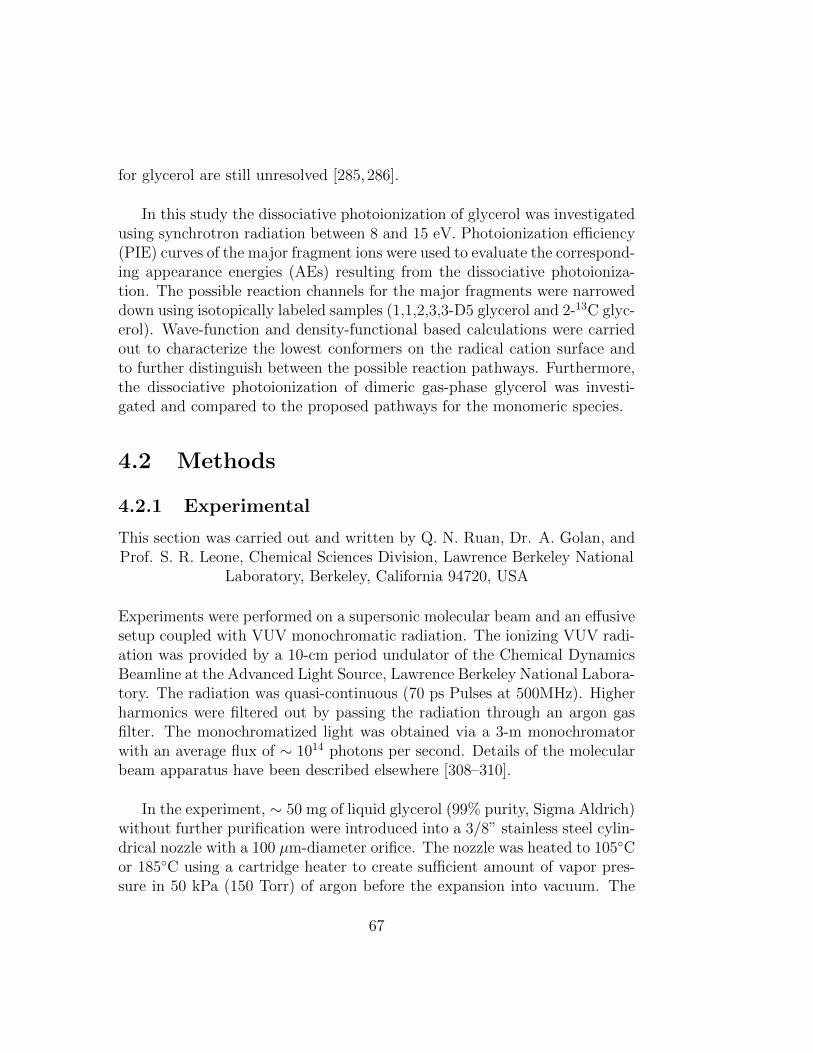
for glycerol are still unresolved [285,286].
In this study the dissociative photoionization of glycerol was investigatedusing synchrotron radiation between 8 and 15 eV. Photoionization efficiency(PIE) curves of the major fragment ions were used to evaluate the correspond-ing appearance energies (AEs) resulting from the dissociative photoioniza-tion. The possible reaction channels for the major fragments were narroweddown using isotopically labeled samples (1,1,2,3,3-D5 glycerol and 2-13C glyc-erol). Wave-function and density-functional based calculations were carriedout to characterize the lowest conformers on the radical cation surface andto further distinguish between the possible reaction pathways. Furthermore,the dissociative photoionization of dimeric gas-phase glycerol was investi-gated and compared to the proposed pathways for the monomeric species.
4.2 Methods
4.2.1 Experimental
This section was carried out and written by Q. N. Ruan, Dr. A. Golan, andProf. S. R. Leone, Chemical Sciences Division, Lawrence Berkeley National
Laboratory, Berkeley, California 94720, USA
Experiments were performed on a supersonic molecular beam and an effusivesetup coupled with VUV monochromatic radiation. The ionizing VUV radi-ation was provided by a 10-cm period undulator of the Chemical DynamicsBeamline at the Advanced Light Source, Lawrence Berkeley National Labora-tory. The radiation was quasi-continuous (70 ps Pulses at 500MHz). Higherharmonics were filtered out by passing the radiation through an argon gasfilter. The monochromatized light was obtained via a 3-m monochromatorwith an average flux of ∼ 1014 photons per second. Details of the molecularbeam apparatus have been described elsewhere [308–310].
In the experiment, ∼ 50 mg of liquid glycerol (99% purity, Sigma Aldrich)without further purification were introduced into a 3/8” stainless steel cylin-drical nozzle with a 100 µm-diameter orifice. The nozzle was heated to 105◦Cor 185◦C using a cartridge heater to create sufficient amount of vapor pres-sure in 50 kPa (150 Torr) of argon before the expansion into vacuum. The
67
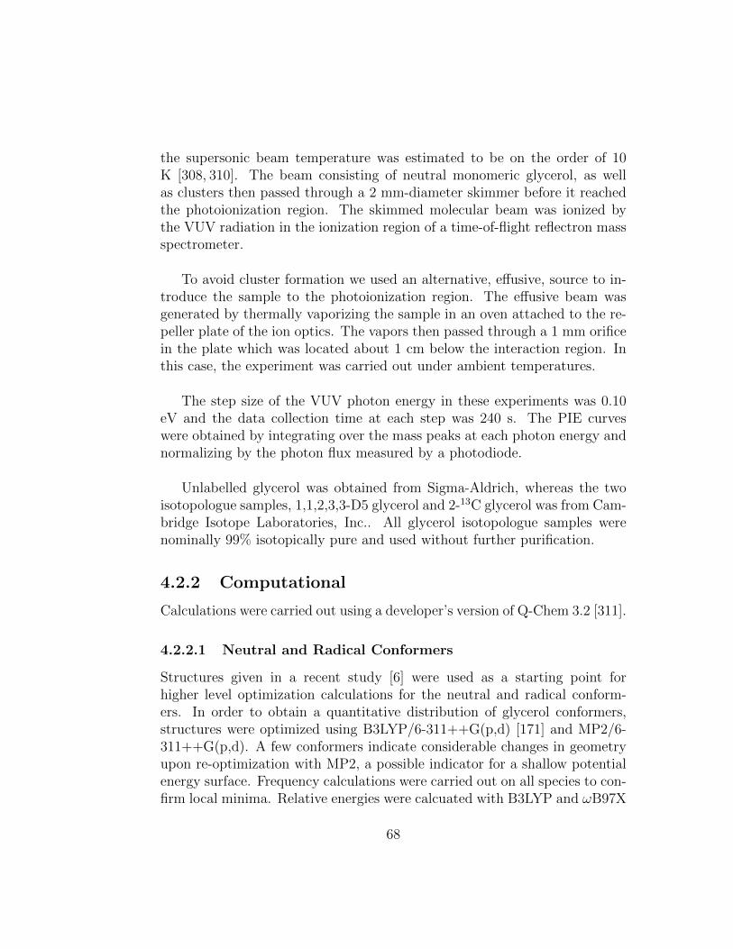
the supersonic beam temperature was estimated to be on the order of 10K [308, 310]. The beam consisting of neutral monomeric glycerol, as wellas clusters then passed through a 2 mm-diameter skimmer before it reachedthe photoionization region. The skimmed molecular beam was ionized bythe VUV radiation in the ionization region of a time-of-flight reflectron massspectrometer.
To avoid cluster formation we used an alternative, effusive, source to in-troduce the sample to the photoionization region. The effusive beam wasgenerated by thermally vaporizing the sample in an oven attached to the re-peller plate of the ion optics. The vapors then passed through a 1 mm orificein the plate which was located about 1 cm below the interaction region. Inthis case, the experiment was carried out under ambient temperatures.
The step size of the VUV photon energy in these experiments was 0.10eV and the data collection time at each step was 240 s. The PIE curveswere obtained by integrating over the mass peaks at each photon energy andnormalizing by the photon flux measured by a photodiode.
Unlabelled glycerol was obtained from Sigma-Aldrich, whereas the twoisotopologue samples, 1,1,2,3,3-D5 glycerol and 2-13C glycerol was from Cam-bridge Isotope Laboratories, Inc.. All glycerol isotopologue samples werenominally 99% isotopically pure and used without further purification.
4.2.2 Computational
Calculations were carried out using a developer’s version of Q-Chem 3.2 [311].
4.2.2.1 Neutral and Radical Conformers
Structures given in a recent study [6] were used as a starting point forhigher level optimization calculations for the neutral and radical conform-ers. In order to obtain a quantitative distribution of glycerol conformers,structures were optimized using B3LYP/6-311++G(p,d) [171] and MP2/6-311++G(p,d). A few conformers indicate considerable changes in geometryupon re-optimization with MP2, a possible indicator for a shallow potentialenergy surface. Frequency calculations were carried out on all species to con-firm local minima. Relative energies were calcuated with B3LYP and ωB97X
68
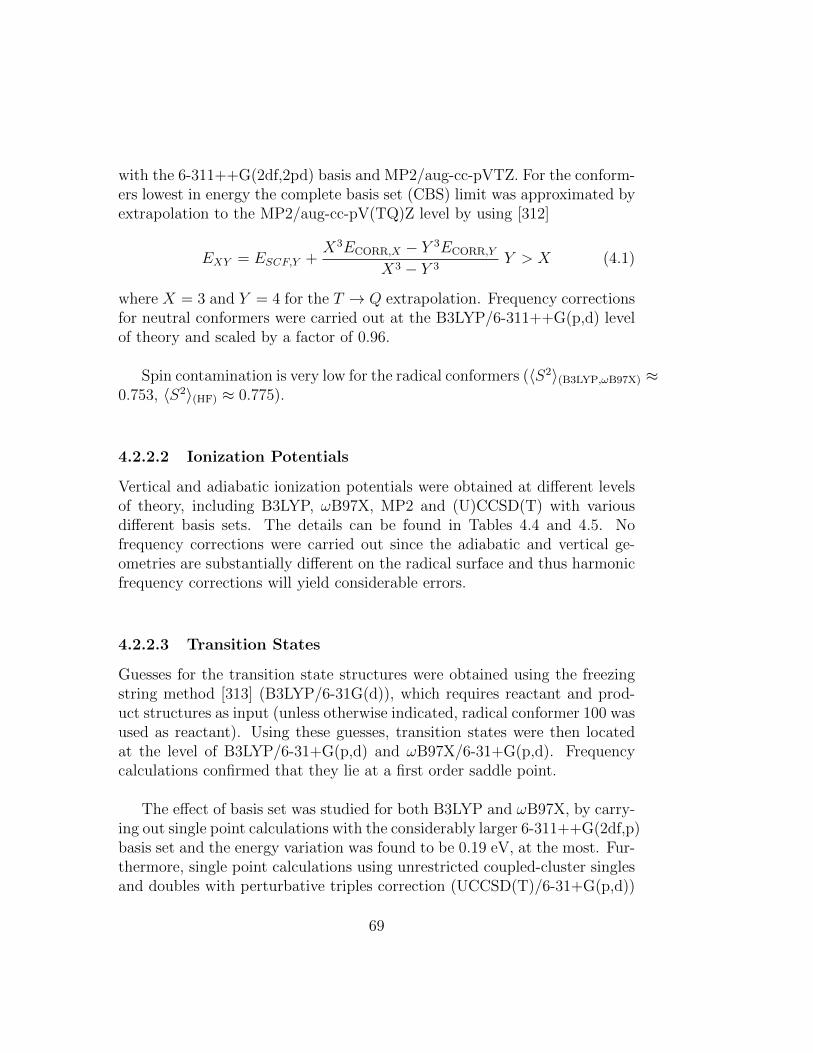
with the 6-311++G(2df,2pd) basis and MP2/aug-cc-pVTZ. For the conform-ers lowest in energy the complete basis set (CBS) limit was approximated byextrapolation to the MP2/aug-cc-pV(TQ)Z level by using [312]
EXY = ESCF,Y +X3ECORR,X − Y 3ECORR,Y
X3 − Y 3Y > X (4.1)
where X = 3 and Y = 4 for the T → Q extrapolation. Frequency correctionsfor neutral conformers were carried out at the B3LYP/6-311++G(p,d) levelof theory and scaled by a factor of 0.96.
Spin contamination is very low for the radical conformers (〈S2〉(B3LYP,ωB97X) ≈0.753, 〈S2〉(HF) ≈ 0.775).
4.2.2.2 Ionization Potentials
Vertical and adiabatic ionization potentials were obtained at different levelsof theory, including B3LYP, ωB97X, MP2 and (U)CCSD(T) with variousdifferent basis sets. The details can be found in Tables 4.4 and 4.5. Nofrequency corrections were carried out since the adiabatic and vertical ge-ometries are substantially different on the radical surface and thus harmonicfrequency corrections will yield considerable errors.
4.2.2.3 Transition States
Guesses for the transition state structures were obtained using the freezingstring method [313] (B3LYP/6-31G(d)), which requires reactant and prod-uct structures as input (unless otherwise indicated, radical conformer 100 wasused as reactant). Using these guesses, transition states were then locatedat the level of B3LYP/6-31+G(p,d) and ωB97X/6-31+G(p,d). Frequencycalculations confirmed that they lie at a first order saddle point.
The effect of basis set was studied for both B3LYP and ωB97X, by carry-ing out single point calculations with the considerably larger 6-311++G(2df,p)basis set and the energy variation was found to be 0.19 eV, at the most. Fur-thermore, single point calculations using unrestricted coupled-cluster singlesand doubles with perturbative triples correction (UCCSD(T)/6-31+G(p,d))
69

were carried out using the frozen core approximation. Finally, transitionstate structures were followed by intrinsic reaction coordinate calculations(IRC) [314] in mass-weighted coordinates toward reactants and products.
4.2.2.4 Choice of Functional
The well-known self-interaction problem [181] may lead to errors in energiesand bond lengths when using the still widely popular B3LYP functional. Al-though self-interaction is not fully resolved in ωB97X [315], it is known tovastly improve upon B3LYP and has recently been shown to yield an ∼ 2.5smaller average mean unsigned deviation in transition state geometries whentested on the TSG48 set [316].
4.2.2.5 Dimeric Glycerol
Glycerol dimer conformers were obtained by performing a molecular mechan-ics conformer search in Spartan [317] using the Merck Molecular Force field(MMFF) [318] in combination with three Monte-Carlo runs, each startingfrom different points and which were terminated after 2000 steps. 100 con-formers were retained in the simulation. Finally the lowest 50 conformerswere selected and re-optimized using B3LYP/6-311++G(p,d).
4.3 Results and Discussion
4.3.1 Experimental Measurements
This section was carried out and written by Q. N. Ruan, Dr. A. Golan, andProf. S. R. Leone, Chemical Sciences Division, Lawrence Berkeley National
Laboratory, Berkeley, California 94720, USA
Figure 4.1(a) shows the dissociative photoionization mass spectrum of glyc-erol at 10.5 eV. The major fragment ions have m/z = 44, 45, 60, 61, 62and 74. Due to the energetic preference of forming intermolecular ratherthan intramolecular hydrogen bonds in glycerol, extensive cluster formationoccurs in the supersonic expansion process, and ion clusters of various sizesare observed in the mass spectrum. However, no ion clusters are detected
70

under effusive conditions (Figure 4.1(b)) as a result of the low likelihood offorming dimeric glycerol species (or higher order clusters) in the vaporizationprocess. The parent signal (92 m/z) is of very low intensity compared to thelower m/z fragment ions.
Figure 4.1(c) shows the dissociative photoionization mass spectrum ofD5 glycerol using the effusive beam method and a photon energy of 10.5eV. A wider range of m/z species are present in the mass spectrum usingD5-glycerol compared to the non-labeled glycerol sample. By matching thePIE patterns and tracing the labeled atoms, more information about thedissociative photoionization pathways can be obtained. As expected, themass spectra of 13C-glycerol are very similar to the ones derived from unla-beled glycerol except that almost every peak is shifted one amu higher dueto one extra neutron in 13C. However, a closer look reveals that the peaksat m/z = 31 and 33 are unaffected. This implies that fragment ions CH3O+
and CH5O+ are derived from the terminal carbons in glycerol. Furthermore,there are two peaks of equivalent intensity at m/z =15 and 16. Comparingthe PIE curves for m/z =15 and 16 indicates that these two peaks are due toa methyl fragment. This suggests that the fragmentation to CH+
3 is unselec-tive and occurs at both the terminal and central carbon. Detailed discussionsof these findings are presented in the next section.
Figure 4.2 shows the PIE curves of (a) the parent ion C3H8O+3 (m/z = 92)
and of the major fragment ions C3H6O+2 (m/z = 74), C2H6O+
2 (m/z = 62),C2H4O+(m/z = 44) (b, c, d, respectively). The PIE curves obtained fromthe supersonic expansion molecular beam and effusive molecular source for aparticular fragment ion are rescaled to fit in the same figure for comparison(Figure 4.2).
The AE for each PIE curve can be determined by using a linear leastsquares fit in the threshold region [319,320] and are listed in Table 4.1. Thesimilarity of the PIE curves and corresponding AEs for both types of molec-ular beams indicates that the photofragment ions with m/z < 92 originatefrom monomeric glycerol in both experimental settings.
71

Figure 4.1: Photoionization TOF mass spectrum of glycerol in (a) supersonicexpansion, (b) effusive source and (c) D5-glycerol in a effusive source at 10.5eV
72
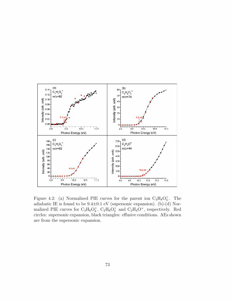
Figure 4.2: (a) Normalized PIE curves for the parent ion C3H8O+3 . The
adiabatic IE is found to be 9.4±0.1 eV (supersonic expansion). (b)-(d) Nor-malized PIE curves for C3H6O+
2 , C2H6O+2 and C2H4O+, respectively. Red
circles: supersonic expansion, black triangles: effusive conditions. AEs shownare from the supersonic expansion.
73

Tab
le4.
1:A
pp
eara
nce
ener
gies
(in
eV±
0.1)
mea
sure
din
the
dis
soci
ativ
ephot
oion
izat
ion
ofgl
yce
rol
and
the
corr
esp
ondin
gfr
agm
ent
ions
ofit
sis
otop
olog
ues
.B
ecau
seof
bac
kgr
ound
wat
erin
the
cham
ber
,th
eot
her
m/z
=18
isom
erC
D+ 3
could
not
be
mea
sure
dfr
omth
eP
IEcu
rve.
Gly
cero
l2-
13C
glyce
rol
D5-
glyce
rol
Ions
(m/z
)A
E(e
V)
Ions
(m/z
)A
E(e
V)
Ions
(m/z
)A
E(e
V)
C3H
8O
+ 3(9
2)A
dia
bat
ic9.
4C
3H
6O
+ 2(7
4)9.
813C
C2H
6O
+ 2(7
5)9.
8C
3H
D5O
+ 2(7
9)9.
9C
2H
6O
+ 2(6
2)9.
913C
CH
6O
+ 2(6
3)10
.0C
2D
4H
2O
+ 2(6
6)M
inor
(1)
10.0
C2D
3H
3O
+ 2(6
5)M
ajo
r(8
)9.
9C
2H
5O
+ 2(6
1)10
.313C
CH
5O
+ 2(6
2)10
.3C
2D
3H
2O
+ 2(6
4)10
.3C
2H
4O
+ 2(6
0)10
.013C
CH
4O
+ 2(6
1)10
.0C
2D
3H
O+ 2
(63)
Min
or(1
)10
.1C
2D
2H
2O
+ 2(6
2)M
ajo
r(2
.3)
10.1
C2H
5O
+(4
5)10
.013C
CH
5O
+(4
6)10
.0C
2D
4H
O+
(49)
10.0
C2H
4O
+(4
4)10
.313C
CH
4O
+(4
5)10
.3C
2D
3H
O+
(47)
10.2
C2H
3O
+(4
3)12
.413C
CH
3O
+(4
4)12
.6C
2D
3O
+(4
6)12
.5C
H5O
+(3
3)11
.0C
H5O
+(3
3)11
.2C
H2D
3O
+(3
6)11
.2C
H3O
+(3
1)11
.4C
H3O
+(3
1)11
.4C
D2H
O+
(33)
11.2
CH
O+
(29)
12.7
13C
HO
+(3
0)12
.6C
DO
+(3
0)12
.6C
2H
+ 4(2
8)11
.113C
CH
+ 4(2
9)11
.2C
2D
+ 4(3
2)11
.0H
2D
O+
(20)
12.5
HD
O+
(19)
12.5
CH
+ 3(1
5)14
.013C
H+ 3
(16)
14.0
CH
+ 3(1
5)14
.0
74

4.3.2 Monomeric Glycerol
4.3.2.1 Neutral Conformers
An extensive conformer search of neutral glycerol has been carried out pre-viously [6]. Relative energies as well as conformer distributions at 10 K and298 K are given in Tables 4.2 and 4.3 based on the most accurate methodsin the prior study. Furthermore, we carried out MP2 T → Q extrapola-tions to approximate MP2 results at the complete basis set limit. Addingfrequency corrections (B3LYP/6-311++G(p,d)), reduces the relative energydifferences between the conformers considerably and changes the ordering ofthe two lowest structures, which are shown in Figure 4.3.
Table 4.2: Relative energies of the lowest neutral gas-phase conformers. Con-former labelling adopted from [6]. The MP2-TQ-extrapolation was carriedout on B3LYP/6-311++G(p,d) geometries. (freq) indicates frequency cor-rected MP2-TQ-extrapolated values.
Conformer G2(MP2)1 CBS-QB31 MP2-TQ (freq)100 0.00 0.00 0.00 (0.00)95 0.21 0.17 0.38 (-0.06)46 0.61 0.75 0.87 (0.25)101 0.64 0.61 0.83 (0.19)109 0.79 0.69 1.11 (0.19)48 1.06 1.09 1.43 (0.77)7 1.09 1.22 1.47 (0.57)45 1.50 1.50 2.01 (1.41)43 1.52 1.72 1.97 (1.21)120 1.54 1.66 2.20 (1.01)34 2.62 1.88 2.63 (1.08)
Table 4.3: Ratio of the two lowest lying conformers 100 : 95 at the experi-mental temperatures
T/K G2(MP2) CBS-QB3 MP2-TQ MP2-TQ(freq)10 4∗104 : 1 5∗103 : 1 2∗108 : 1 1 : 2∗101
298 1.4 : 1 1.3 : 1 1.9 : 1 1 : 1.1
75
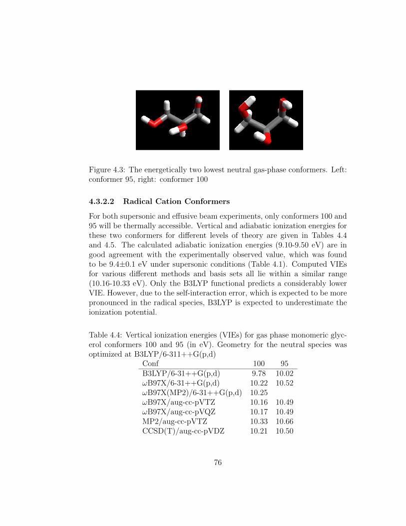
Figure 4.3: The energetically two lowest neutral gas-phase conformers. Left:conformer 95, right: conformer 100
4.3.2.2 Radical Cation Conformers
For both supersonic and effusive beam experiments, only conformers 100 and95 will be thermally accessible. Vertical and adiabatic ionization energies forthese two conformers for different levels of theory are given in Tables 4.4and 4.5. The calculated adiabatic ionization energies (9.10-9.50 eV) are ingood agreement with the experimentally observed value, which was foundto be 9.4±0.1 eV under supersonic conditions (Table 4.1). Computed VIEsfor various different methods and basis sets all lie within a similar range(10.16-10.33 eV). Only the B3LYP functional predicts a considerably lowerVIE. However, due to the self-interaction error, which is expected to be morepronounced in the radical species, B3LYP is expected to underestimate theionization potential.
Table 4.4: Vertical ionization energies (VIEs) for gas phase monomeric glyc-erol conformers 100 and 95 (in eV). Geometry for the neutral species wasoptimized at B3LYP/6-311++G(p,d)
Conf 100 95B3LYP/6-31++G(p,d) 9.78 10.02ωB97X/6-31++G(p,d) 10.22 10.52ωB97X(MP2)/6-31++G(p,d) 10.25ωB97X/aug-cc-pVTZ 10.16 10.49ωB97X/aug-cc-pVQZ 10.17 10.49MP2/aug-cc-pVTZ 10.33 10.66CCSD(T)/aug-cc-pVDZ 10.21 10.50
76
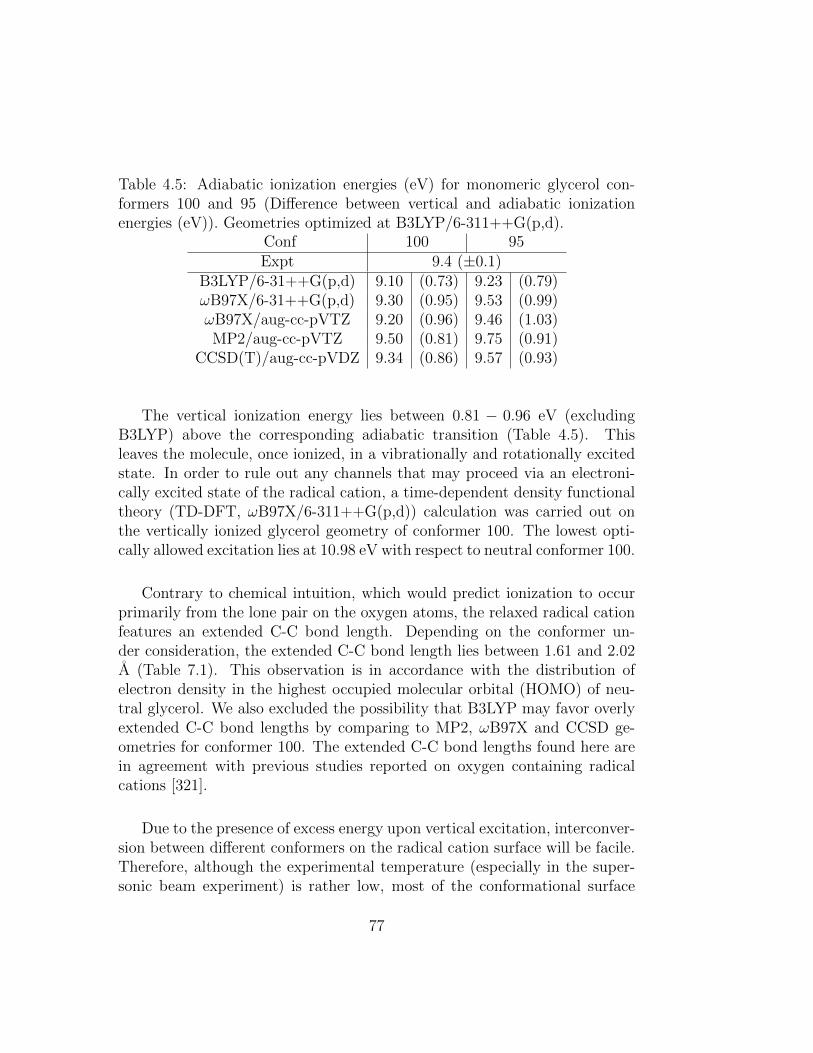
Table 4.5: Adiabatic ionization energies (eV) for monomeric glycerol con-formers 100 and 95 (Difference between vertical and adiabatic ionizationenergies (eV)). Geometries optimized at B3LYP/6-311++G(p,d).
Conf 100 95Expt 9.4 (±0.1)
B3LYP/6-31++G(p,d) 9.10 (0.73) 9.23 (0.79)ωB97X/6-31++G(p,d) 9.30 (0.95) 9.53 (0.99)ωB97X/aug-cc-pVTZ 9.20 (0.96) 9.46 (1.03)MP2/aug-cc-pVTZ 9.50 (0.81) 9.75 (0.91)
CCSD(T)/aug-cc-pVDZ 9.34 (0.86) 9.57 (0.93)
The vertical ionization energy lies between 0.81 − 0.96 eV (excludingB3LYP) above the corresponding adiabatic transition (Table 4.5). Thisleaves the molecule, once ionized, in a vibrationally and rotationally excitedstate. In order to rule out any channels that may proceed via an electroni-cally excited state of the radical cation, a time-dependent density functionaltheory (TD-DFT, ωB97X/6-311++G(p,d)) calculation was carried out onthe vertically ionized glycerol geometry of conformer 100. The lowest opti-cally allowed excitation lies at 10.98 eV with respect to neutral conformer 100.
Contrary to chemical intuition, which would predict ionization to occurprimarily from the lone pair on the oxygen atoms, the relaxed radical cationfeatures an extended C-C bond length. Depending on the conformer un-der consideration, the extended C-C bond length lies between 1.61 and 2.02A (Table 7.1). This observation is in accordance with the distribution ofelectron density in the highest occupied molecular orbital (HOMO) of neu-tral glycerol. We also excluded the possibility that B3LYP may favor overlyextended C-C bond lengths by comparing to MP2, ωB97X and CCSD ge-ometries for conformer 100. The extended C-C bond lengths found here arein agreement with previous studies reported on oxygen containing radicalcations [321].
Due to the presence of excess energy upon vertical excitation, interconver-sion between different conformers on the radical cation surface will be facile.Therefore, although the experimental temperature (especially in the super-sonic beam experiment) is rather low, most of the conformational surface
77

will be accessible to the radical cation. The results of an extensive conforma-tional search on the radical cation surface is given in the Appendix (Tables7.1 and 7.2). The conformers can be subgrouped based on their geometricalparameters, such as relative C-C bond lengths and the presence of hydrogenbonds. Cartoons for representatives of each of these main sub-classes aredepicted in Figure 4.4 and their geometrical parameters and relative energiesare given in Tables 4.6 and 4.7, along with the 10 lowest lying conformers.Due to self-interaction errors, B3LYP and ωB97X differ most (between 1.1and 3.8 kcal/mol) for those conformers where the two C-C bond lengths andspin densities on the carbon atoms are similar. Otherwise, the two func-tionals are in very good agreement and differ by 0.45 kcal/mol at the most(Appendix, Table 7.2).
Although the relative ordering changes between different methods, allof them predict that the lowest ten gas-phase monomeric radical cation con-formers are 2, 34, 43, 48, 66, 67, 80, 100, 101 and 109. All of these conformershave the same geometric features: A hydrogen bond between the central andthe terminal OH groups, and one very long and one short C-C bond.
78
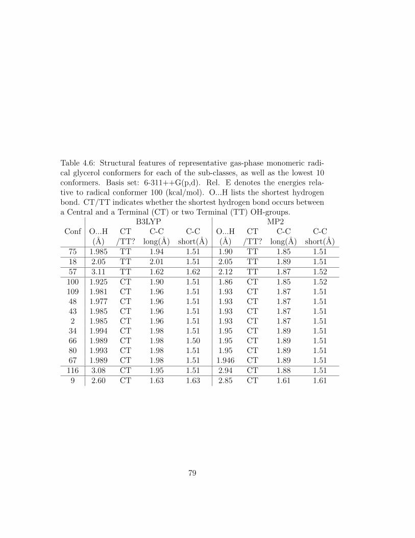
Table 4.6: Structural features of representative gas-phase monomeric radi-cal glycerol conformers for each of the sub-classes, as well as the lowest 10conformers. Basis set: 6-311++G(p,d). Rel. E denotes the energies rela-tive to radical conformer 100 (kcal/mol). O...H lists the shortest hydrogenbond. CT/TT indicates whether the shortest hydrogen bond occurs betweena Central and a Terminal (CT) or two Terminal (TT) OH-groups.
B3LYP MP2Conf O...H CT C-C C-C O...H CT C-C C-C
(A) /TT? long(A) short(A) (A) /TT? long(A) short(A)75 1.985 TT 1.94 1.51 1.90 TT 1.85 1.5118 2.05 TT 2.01 1.51 2.05 TT 1.89 1.5157 3.11 TT 1.62 1.62 2.12 TT 1.87 1.52100 1.925 CT 1.90 1.51 1.86 CT 1.85 1.52109 1.981 CT 1.96 1.51 1.93 CT 1.87 1.5148 1.977 CT 1.96 1.51 1.93 CT 1.87 1.5143 1.985 CT 1.96 1.51 1.93 CT 1.87 1.512 1.985 CT 1.96 1.51 1.93 CT 1.87 1.5134 1.994 CT 1.98 1.51 1.95 CT 1.89 1.5166 1.989 CT 1.98 1.50 1.95 CT 1.89 1.5180 1.993 CT 1.98 1.51 1.95 CT 1.89 1.5167 1.989 CT 1.98 1.51 1.946 CT 1.89 1.51116 3.08 CT 1.95 1.51 2.94 CT 1.88 1.519 2.60 CT 1.63 1.63 2.85 CT 1.61 1.61
79
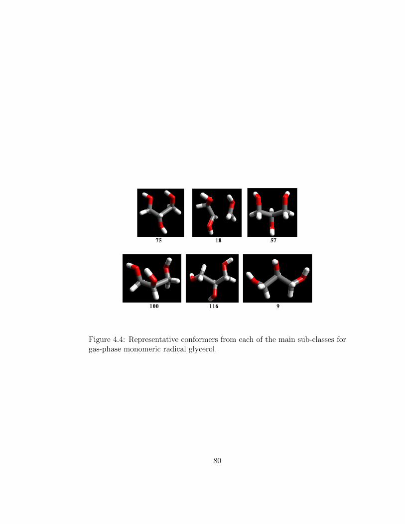
Figure 4.4: Representative conformers from each of the main sub-classes forgas-phase monomeric radical glycerol.
80
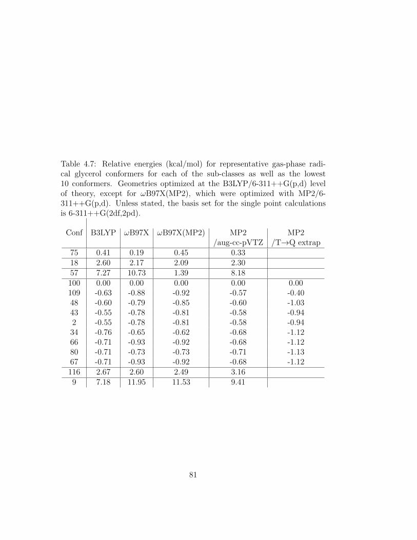
Table 4.7: Relative energies (kcal/mol) for representative gas-phase radi-cal glycerol conformers for each of the sub-classes as well as the lowest10 conformers. Geometries optimized at the B3LYP/6-311++G(p,d) levelof theory, except for ωB97X(MP2), which were optimized with MP2/6-311++G(p,d). Unless stated, the basis set for the single point calculationsis 6-311++G(2df,2pd).
Conf B3LYP ωB97X ωB97X(MP2) MP2 MP2/aug-cc-pVTZ /T→Q extrap
75 0.41 0.19 0.45 0.3318 2.60 2.17 2.09 2.3057 7.27 10.73 1.39 8.18100 0.00 0.00 0.00 0.00 0.00109 -0.63 -0.88 -0.92 -0.57 -0.4048 -0.60 -0.79 -0.85 -0.60 -1.0343 -0.55 -0.78 -0.81 -0.58 -0.942 -0.55 -0.78 -0.81 -0.58 -0.9434 -0.76 -0.65 -0.62 -0.68 -1.1266 -0.71 -0.93 -0.92 -0.68 -1.1280 -0.71 -0.73 -0.73 -0.71 -1.1367 -0.71 -0.93 -0.92 -0.68 -1.12116 2.67 2.60 2.49 3.169 7.18 11.95 11.53 9.41
81
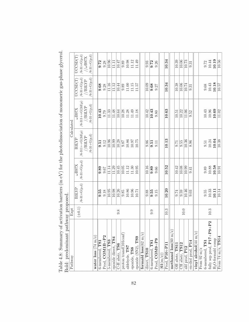
Tab
le4.
8:Sum
mar
yof
acti
vati
onbar
rier
s(i
neV
)fo
rth
ephot
odis
soci
atio
nof
mon
omer
icga
s-phas
egl
yce
rol.
Bol
d:
pre
dom
inan
tpat
hw
aypro
pos
ed.
Pat
hw
ayE
xp
tC
alcu
late
d
(±0.
1)B
3LY
Pω
B97
XB
3LY
Pω
B97
XU
CC
SD
(T)
UC
CS
D(T
)/6-31+G(p,d)
/6-31+G(p,d)
/6-311+
+G(2df,p)
/6-311++G(2df,p)
/6-31+G(p,d)
/6-31+
G(p,d)
//B
3LY
P//
B3L
YP
//B
3LY
P//ω
B97
X/6-31+G(p,d)
/6-31+
G(p,d)
/6-31+G(p,d)
/6-31+
G(p,d)
wate
rlo
ss(7
4m
/z)
6-m
emb
ered
,T
S1
9.8
9.5
59.8
99.5
110.4
39.6
89.7
2P
rod
,C
OM
1B
+P
29.
189.
679.
129.
799.
289.
285-
mem
ber
ed,T
S3
10.9
511
.14
10.9
611
.33
11.1
610
.96
epox
ide
dir
ect,
TS4
10.9
811
.29
10.9
911
.48
11.1
211
.11
C-H
abst
r,T
S6
10.2
610
.45
10.2
810
.64
10.4
410
.47
pro
ton
tran
sf(1
01co
nf)
9.85
10.0
59.
8710
.28
9.89
9.89
ald
ehyd
e,T
S7
10.8
611
.12
10.8
611
.28
11.0
010
.98
epox
ide,
TS8
10.9
611
.30
10.9
711
.49
11.1
511
.12
epox
ide
(SN
2),T
S9
10.7
110
.95
10.7
511
.18
11.5
711
.49
form
ald
loss
(62
m/z
)d
irec
t,T
S10
9.9
9.88
10.1
69.
8610
.42
10.0
99.
936-
mem
ber
ed,T
S1
9.5
59.8
99.5
110.4
39.6
89.7
2P
rod
,C
OM
9+
P9
9.15
9.66
9.11
9.80
9.27
9.26
(61
(m/z
))P
rod
,P
10
+P
11
10.3
10.2
010.5
210.1
310.6
310.3
410.3
4
meth
anol
loss
(60
m/z
)O
Hab
str,
TS11
10.0
9.74
10.4
29.
7110
.51
10.3
810
.39
CH
abst
r,T
S12
9.59
10.0
89.
5510
.22
10.0
610
.06
ald
pro
d,P
12
10.4
610
.99
10.3
611
.06
10.7
410
.73
en-d
iol
pro
d,P
14
9.03
9.41
8.96
9.52
9.31
9.31
vin
yl
alc
ohol(
44m
/z)
Fro
m92
m/z
10.3
6-m
emb
ered
,T
S1
9.55
9.89
9.51
10.4
39.
689.
72fu
lly
sep
pro
d,P
17
+P
9+
P2
10.3
310
.88
10.2
410
.96
10.4
310
.44
H2O
-for
mal
dco
mp
10.1
110.5
810.0
410.6
910.1
810.1
9F
rom
74m
/z,T
S14
10.1
410
.91
10.3
811
.02
10.5
710
.56
82
4.3.2.3 Water Loss (74 m/z)
Although absent in ethylene glycol [322], water loss from the parent ion(92 m/z) is the lowest energy channel observed experimentally in glycerol(9.8±0.1 eV, Table 4.1) and is responsible for the C3H6O+
2 (74 m/z) peak inthe mass spectrum.
Proposed MechanismBased on our computations and experimental data, we propose a 6-memberedproton-transfer transition state to be responsible for water loss, which is pro-moted by hydrogen bonding between the two terminal OH groups. The re-sulting concerted reaction (Figure 4.5) results in a product complex involvingwater (18 m/z), formaldehyde (30 m/z) and vinyl alcohol radical (44 m/z)(COM1A, Figure 4.5). This channel features a very low barrier, as the ratelimiting step is proton transfer between the two terminal OH groups (TS1,Figure 4.5). Since the C-C framework is weakened due to ionization, energypenalties due to deformations in the carbon backbone are small. Althoughat first glance, this channel may be disregarded, as the product resultingfrom water loss has mass 74 m/z, full separation of the products (i.e. hy-drogen bond cleavage and localization of the positive charge and radical onthe vinyl alcohol) requires a substantial amount of energy, as is discussed inmore detail below. However, loss of either neutral water or neutral formalde-hyde preserves one of the hydrogen bonds in the product complex (COM1B,COM9, Figures 4.5 and 4.11) and allows for charge and spin density delo-calization, therefore making water (or formaldehyde) loss substantially lowerin energy. Indeed, calculations show that the rate limiting step in water (orformaldehyde) loss is the transfer of the proton via the 6-membered tran-sition state (9.72 eV, Table 4.8). Water (or formaldehyde) separated fullyfrom the product complex lies at only 9.28 eV (9.26 eV), Table 4.8. Thisalso accounts for the similar appearance energies of formaldehyde and waterseen in the experiment. Also, since proton transfer occurs between two OHgroups, the proposed mechanism for water loss matches the observations inthe deuterium labeling experiments (Table AE). Furthermore, this mecha-nism can account for the absence of a water- and formaldehydeloss peaks inthe mass spectrum for glycerol dimer, as will be discussed in more detail insection 4.3.3.
83
Alternative MechanismsOn paper, a variety of other channels could give rise to water loss in glycerol.We have computed most of these channels, which are schematically shown inFigures 4.6 to 4.8.
Amongst these, we considered a five-membered transition state, whichyields either 3-hydroxypropenal (P3) or hydroxyacetone (P4) as the prod-uct, depending if water loss occurs from the 1- or 2- position (Figure 4.6).
Furthermore, the dehydration of neutral glycerol in the gas phase is pro-posed to take place via glycidol (P5) with an energy barrier of 70.9 kcal/mol(3.07 eV) [289]. Although dissociative photoionization channels are oftenvery different from pyrolysis, we also included this epoxide intermediate inour study (Figures 4.7 and 4.8).
Finally, we were able to locate a low-lying water-bound intermediate(INT1, Figure 4.8), from which several different pathways are possible (Fig-ure 4.8). The first involves a 1,2-hydride shift to yield 3-hydroxypropanal(P3). The other two pathways (TS8, TS9) again yield glycidol as product(P5). The two pathways differ in the attack of the oxygen radical, whichcan take place from the same side to preserve the hydrogen bonding network,or in an SN2 type fashion from the backside. The latter involves a furtherintermediate (INT2), where the oxygen atom now lies on the opposite side.
The energetics for the mechanisms proposed in Figures 4.6 to 4.8 aresummarized in Figure 4.9. As can be seen, most of the barriers displayed inFigure 4.9 lie substantially higher in energy than is observed experimentally.Basis set effects and differences in methods do not have a very large effect onthe energetics, as can be seen from Table 4.8. The only low-lying transitionstate, which coincides with the experimental results besides the 6-memberedpathway (Figure 4.5), involves transfer of a proton from a terminal to thecentral OH group (9.89 eV, UCCSD(T), Table 4.8), forming an intermediate(INT1) that lies 1.46-1.49 eV (ωB97X) below the separated products (0.32-0.79 eV below the product complex, Figure 4.9), depending on the mecha-nism under consideration. Interestingly, this intermediate cannot be directlyformed from the vertically excited conformer 100, as the hydrogen bondingnetwork is set up to transfer a proton from the central to the terminal OHgroup. However, many other low-lying conformers (such as conformer 101)
84
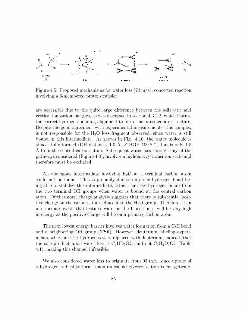
Figure 4.5: Proposed mechanisms for water loss (74 m/z), concerted reactioninvolving a 6-membered proton-transfer
are accessible due to the quite large difference between the adiabatic andvertical ionization energies, as was discussed in section 4.3.2.2, which featurethe correct hydrogen bonding alignment to form this intermediate structure.Despite the good agreement with experimental measurements, this complexis not responsible for the H2O loss fragment observed, since water is stillbound in this intermediate. As shown in Fig. 4.10, the water molecule isalmost fully formed (OH distances 1.0 A, ∠ HOH 109.8 ◦), but is only 1.5A from the central carbon atom. Subsequent water loss through any of thepathways considered (Figure 4.8), involves a high-energy transition state andtherefore must be excluded.
An analogous intermediate involving H2O at a terminal carbon atomcould not be found. This is probably due to only one hydrogen bond be-ing able to stabilize this intermediate, rather than two hydrogen bonds fromthe two terminal OH groups when water is bound at the central carbonatom. Furthermore, charge analysis suggests that there is substantial posi-tive charge on the carbon atom adjacent to the H2O group. Therefore, if anintermediate exists that features water in the 1-position it will be very highin energy as the positive charge will be on a primary carbon atom.
The next lowest energy barrier involves water formation from a C-H bondand a neighboring OH group (TS6). However, deuterium labeling experi-ments, where all C-H hydrogens were replaced with deuterium, indicate thatthe sole product upon water loss is C3HD5O+
2 , and not C3H2D4O+2 (Table
4.1), making this channel infeasible.
We also considered water loss to originate from 93 m/z, since uptake ofa hydrogen radical to form a non-radicaloid glycerol cation is energetically
85
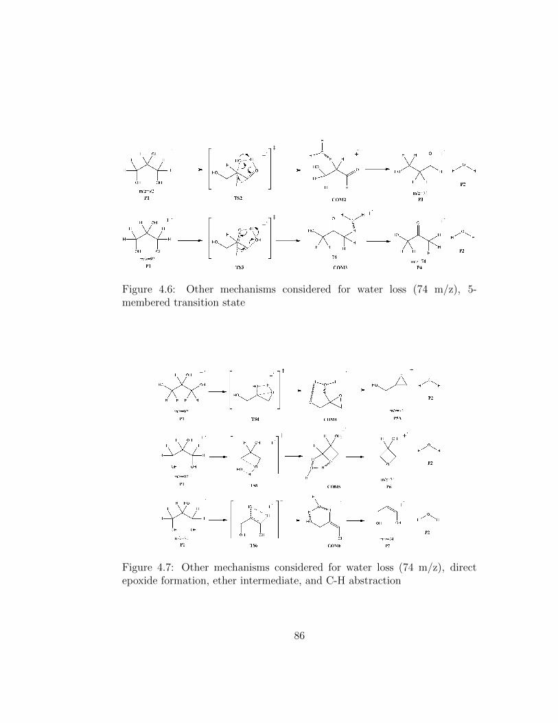
Figure 4.6: Other mechanisms considered for water loss (74 m/z), 5-membered transition state
Figure 4.7: Other mechanisms considered for water loss (74 m/z), directepoxide formation, ether intermediate, and C-H abstraction
86
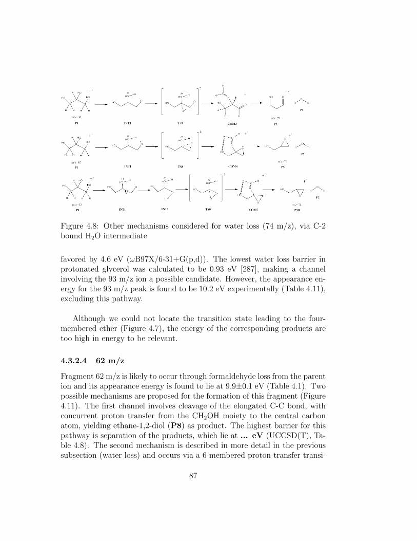
Figure 4.8: Other mechanisms considered for water loss (74 m/z), via C-2bound H2O intermediate
favored by 4.6 eV (ωB97X/6-31+G(p,d)). The lowest water loss barrier inprotonated glycerol was calculated to be 0.93 eV [287], making a channelinvolving the 93 m/z ion a possible candidate. However, the appearance en-ergy for the 93 m/z peak is found to be 10.2 eV experimentally (Table 4.11),excluding this pathway.
Although we could not locate the transition state leading to the four-membered ether (Figure 4.7), the energy of the corresponding products aretoo high in energy to be relevant.
4.3.2.4 62 m/z
Fragment 62 m/z is likely to occur through formaldehyde loss from the parention and its appearance energy is found to lie at 9.9±0.1 eV (Table 4.1). Twopossible mechanisms are proposed for the formation of this fragment (Figure4.11). The first channel involves cleavage of the elongated C-C bond, withconcurrent proton transfer from the CH2OH moiety to the central carbonatom, yielding ethane-1,2-diol (P8) as product. The highest barrier for thispathway is separation of the products, which lie at ... eV (UCCSD(T), Ta-ble 4.8). The second mechanism is described in more detail in the previoussubsection (water loss) and occurs via a 6-membered proton-transfer transi-
87
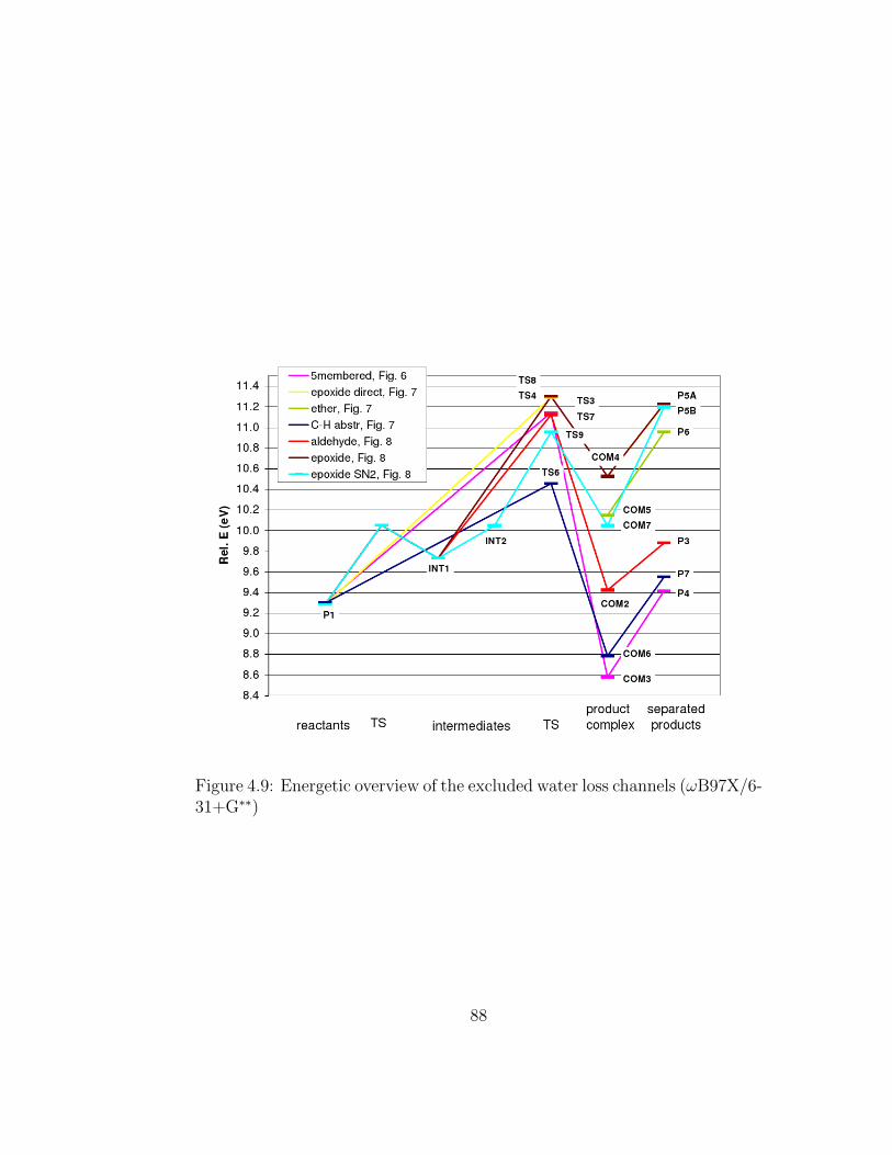
Figure 4.9: Energetic overview of the excluded water loss channels (ωB97X/6-31+G∗∗)
88
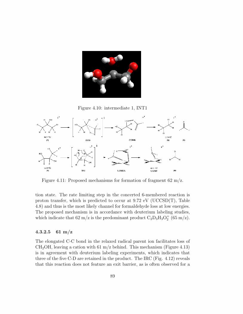
Figure 4.10: intermediate 1, INT1
Figure 4.11: Proposed mechanisms for formation of fragment 62 m/z.
tion state. The rate limiting step in the concerted 6-membered reaction isproton transfer, which is predicted to occur at 9.72 eV (UCCSD(T), Table4.8) and thus is the most likely channel for formaldehyde loss at low energies.The proposed mechanism is in accordance with deuterium labeling studies,which indicate that 62 m/z is the predominant product C2D3H3O+
2 (65 m/z).
4.3.2.5 61 m/z
The elongated C-C bond in the relaxed radical parent ion facilitates loss ofCH2OH, leaving a cation with 61 m/z behind. This mechanism (Figure 4.13)is in agreement with deuterium labeling experiments, which indicates thatthree of the five C-D are retained in the product. The IRC (Fig. 4.12) revealsthat this reaction does not feature an exit barrier, as is often observed for a
89
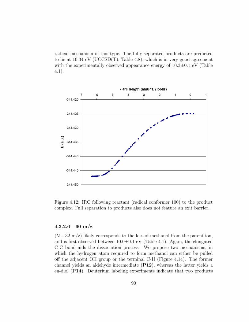
radical mechanism of this type. The fully separated products are predictedto lie at 10.34 eV (UCCSD(T), Table 4.8), which is in very good agreementwith the experimentally observed appearance energy of 10.3±0.1 eV (Table4.1).
Figure 4.12: IRC following reactant (radical conformer 100) to the productcomplex. Full separation to products also does not feature an exit barrier.
4.3.2.6 60 m/z
(M - 32 m/z) likely corresponds to the loss of methanol from the parent ion,and is first observed between 10.0±0.1 eV (Table 4.1). Again, the elongatedC-C bond aids the dissociation process. We propose two mechanisms, inwhich the hydrogen atom required to form methanol can either be pulledoff the adjacent OH group or the terminal C-H (Figure 4.14). The formerchannel yields an aldehyde intermediate (P12), whereas the latter yields aen-diol (P14). Deuterium labeling experiments indicate that two products
90
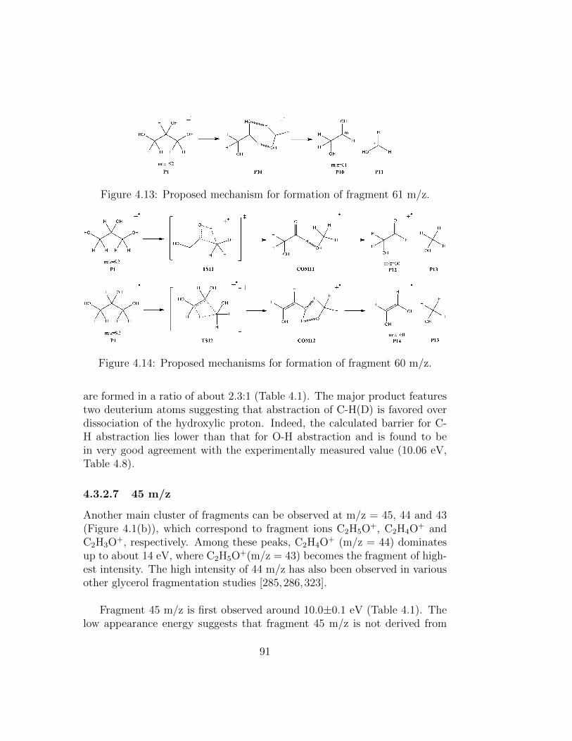
Figure 4.13: Proposed mechanism for formation of fragment 61 m/z.
Figure 4.14: Proposed mechanisms for formation of fragment 60 m/z.
are formed in a ratio of about 2.3:1 (Table 4.1). The major product featurestwo deuterium atoms suggesting that abstraction of C-H(D) is favored overdissociation of the hydroxylic proton. Indeed, the calculated barrier for C-H abstraction lies lower than that for O-H abstraction and is found to bein very good agreement with the experimentally measured value (10.06 eV,Table 4.8).
4.3.2.7 45 m/z
Another main cluster of fragments can be observed at m/z = 45, 44 and 43(Figure 4.1(b)), which correspond to fragment ions C2H5O+, C2H4O+ andC2H3O+, respectively. Among these peaks, C2H4O+ (m/z = 44) dominatesup to about 14 eV, where C2H5O+(m/z = 43) becomes the fragment of high-est intensity. The high intensity of 44 m/z has also been observed in variousother glycerol fragmentation studies [285,286,323].
Fragment 45 m/z is first observed around 10.0±0.1 eV (Table 4.1). Thelow appearance energy suggests that fragment 45 m/z is not derived from
91
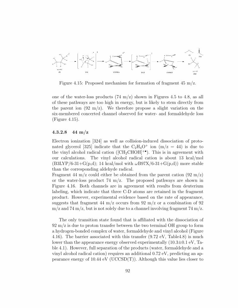
Figure 4.15: Proposed mechanism for formation of fragment 45 m/z.
one of the water-loss products (74 m/z) shown in Figures 4.5 to 4.8, as allof these pathways are too high in energy, but is likely to stem directly fromthe parent ion (92 m/z). We therefore propose a slight variation on thesix-membered concerted channel observed for water- and formaldehyde loss(Figure 4.15).
4.3.2.8 44 m/z
Electron ionization [324] as well as collision-induced dissociation of proto-nated glycerol [325] indicate that the C2H4O+ ion (m/z = 44) is due tothe vinyl alcohol radical cation ([CH2CHOH]+•). This is in agreement withour calculations. The vinyl alcohol radical cation is about 13 kcal/mol(B3LYP/6-31+G(p,d); 14 kcal/mol with ωB97X/6-31+G(p,d)) more stablethan the corresponding aldehyde radical.Fragment 44 m/z could either be obtained from the parent cation (92 m/z)or the water-loss product 74 m/z. The proposed pathways are shown inFigure 4.16. Both channels are in agreement with results from deuteriumlabeling, which indicate that three C-D atoms are retained in the fragmentproduct. However, experimental evidence based on the rate of appearance,suggests that fragment 44 m/z occurs from 92 m/z or a combination of 92m/z and 74 m/z, but is not solely due to a channel involving fragment 74 m/z.
The only transition state found that is affiliated with the dissociation of92 m/z is due to proton transfer between the two terminal OH group to forma hydrogen-bonded complex of water, formaldehyde and vinyl alcohol (Figure4.16). The barrier associated with this transfer (9.72 eV, Table4.8) is muchlower than the appearance energy observed experimentally (10.3±0.1 eV, Ta-ble 4.1). However, full separation of the products (water, formaldehyde and avinyl alcohol radical cation) requires an additional 0.72 eV, predicting an ap-pearance energy of 10.44 eV (UCCSD(T)). Although this value lies closer to
92

Figure 4.16: Proposed mechanisms for water loss (74 m/z), formaldehydeloss (62 m/z) and formation of 44 m/z (vinyl alcohol)
the experimental one, the observed appearance energy is now overestimated.However, if instead of separating all three fragments, a hydrogen-bondedcomplex of water and formaldehyde dissociates to leave fragment 44 m/zbehind, an appearance energy of 10.19 eV is computed (Table 4.8), whichcoincides with the experimental findings.
The barrier affiliated with the rearrangement of 74 m/z is only slightlyhigher than the dissociation to products (10.56 eV, Table4.8). However, thispathway requires formation of the aldehyde water-loss product (Figures 4.6and 4.16) as a starting material, which was found to have >11 eV barrier.This suggests that 44 m/z originates solely from 92 m/z, in accordance withexperimental findings.
4.3.2.9 43 m/z
Previous electron ionization studies [326, 327], indicate that C2H4O+ is amixture of two isomers: one is derived from m/z = 44 (Figure 4.17), whilethe other one is the oxiranyl cation, which results from [CH2OH]• loss ofglycidol P5 (74 m/z). The appearance energy of fragment 43 m/z is foundto be 12.4±0.1 eV (Table 4.1). Since isolated glycidol radical is computed tolie at around 11.2 eV (Table 4.8), the channel starting from 74 m/z cannot beexcluded without further computations. However, experimentally the slope
93
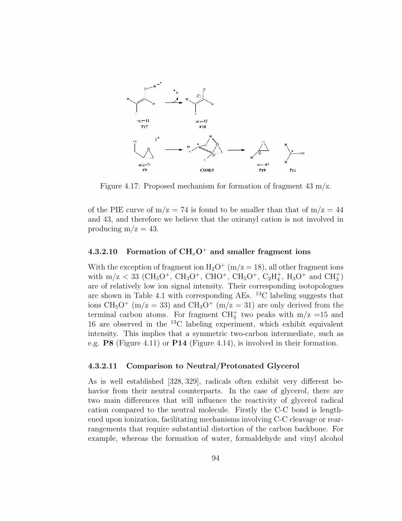
Figure 4.17: Proposed mechanism for formation of fragment 43 m/z.
of the PIE curve of m/z = 74 is found to be smaller than that of m/z = 44and 43, and therefore we believe that the oxiranyl cation is not involved inproducing m/z = 43.
4.3.2.10 Formation of CHxO+ and smaller fragment ions
With the exception of fragment ion H2O+ (m/z = 18), all other fragment ionswith m/z < 33 (CH5O+, CH3O+, CHO+, CH5O+, C2H+
4 , H3O+ and CH+3 )
are of relatively low ion signal intensity. Their corresponding isotopologuesare shown in Table 4.1 with corresponding AEs. 13C labeling suggests thations CH5O+ (m/z = 33) and CH3O+ (m/z = 31) are only derived from theterminal carbon atoms. For fragment CH+
3 two peaks with m/z =15 and16 are observed in the 13C labeling experiment, which exhibit equivalentintensity. This implies that a symmetric two-carbon intermediate, such ase.g. P8 (Figure 4.11) or P14 (Figure 4.14), is involved in their formation.
4.3.2.11 Comparison to Neutral/Protonated Glycerol
As is well established [328, 329], radicals often exhibit very different be-havior from their neutral counterparts. In the case of glycerol, there aretwo main differences that will influence the reactivity of glycerol radicalcation compared to the neutral molecule. Firstly the C-C bond is length-ened upon ionization, facilitating mechanisms involving C-C cleavage or rear-rangements that require substantial distortion of the carbon backbone. Forexample, whereas the formation of water, formaldehyde and vinyl alcohol
94

via a 6-membered transition state requires more than 2.8 eV for the neutralspecies [287], the same reaction requires only 1.30 eV (with respect to theadiabatic structure, conformer 100, ωB97X, Table 4.8) on the radical surface.Furthermore, since glycerol is such a small molecule, full separation of thefinal products, once formed, may require a substantial amount of energy (upto 1.9 eV) and although barriers affiliated with certain rearrangements (suchas proton shifts) may be low, the corresponding products will not be observeduntil much higher energies. This, of course, will be far less pronounced forthe reactions of neutral glycerol.
4.3.3 Dimeric Glycerol
Since glycerol is known to form extensive intermolecular hydrogen bondingnetworks [330–332], we were interested how the dissociative channels are in-fluenced by the presence of a second glycerol molecule.
A conformer search for neutral dimeric glycerol was carried out (see sec-tion 4.2.2.5 for details). The lowest structure is displayed in Figure 4.3.3,and lies 0.71 eV (ωB97X/6-311++G(p,d)//B3LYP/6-311++G(p,d)) belowtwo isolated neutral monomeric glycerol molecules (conformer 100). Table4.9 summarizes the relative energies and some structural parameters of thelowest 10 dimer conformers. The low-lying structures feature mainly inter-molecular rather than intramolecular hydrogen bonds. This is not surprising,as the directionality and distance of intramolecular hydrogen bonds are notas favorable. For the lowest two structures both intramolecular hydrogenbonds are between the two terminal OH groups, which allows each of theglycerol molecules to adopt a chair-like conformation.
95
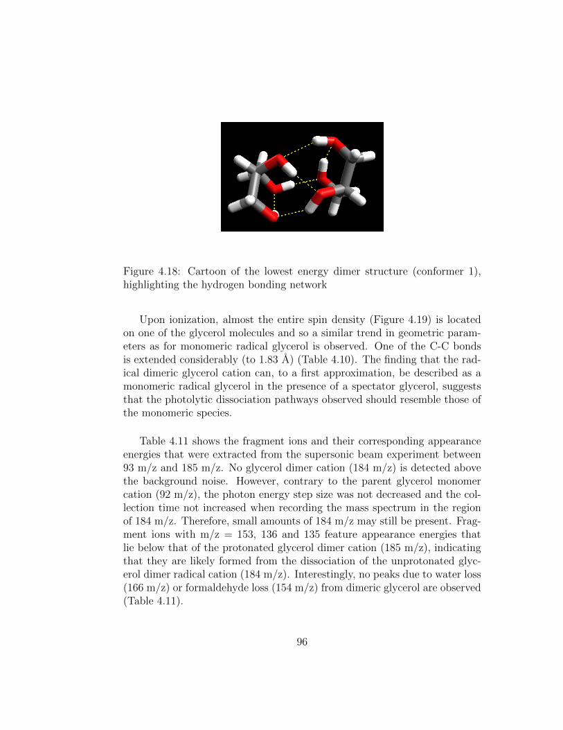
Figure 4.18: Cartoon of the lowest energy dimer structure (conformer 1),highlighting the hydrogen bonding network
Upon ionization, almost the entire spin density (Figure 4.19) is locatedon one of the glycerol molecules and so a similar trend in geometric param-eters as for monomeric radical glycerol is observed. One of the C-C bondsis extended considerably (to 1.83 A) (Table 4.10). The finding that the rad-ical dimeric glycerol cation can, to a first approximation, be described as amonomeric radical glycerol in the presence of a spectator glycerol, suggeststhat the photolytic dissociation pathways observed should resemble those ofthe monomeric species.
Table 4.11 shows the fragment ions and their corresponding appearanceenergies that were extracted from the supersonic beam experiment between93 m/z and 185 m/z. No glycerol dimer cation (184 m/z) is detected abovethe background noise. However, contrary to the parent glycerol monomercation (92 m/z), the photon energy step size was not decreased and the col-lection time not increased when recording the mass spectrum in the regionof 184 m/z. Therefore, small amounts of 184 m/z may still be present. Frag-ment ions with m/z = 153, 136 and 135 feature appearance energies thatlie below that of the protonated glycerol dimer cation (185 m/z), indicatingthat they are likely formed from the dissociation of the unprotonated glyc-erol dimer radical cation (184 m/z). Interestingly, no peaks due to water loss(166 m/z) or formaldehyde loss (154 m/z) from dimeric glycerol are observed(Table 4.11).
96
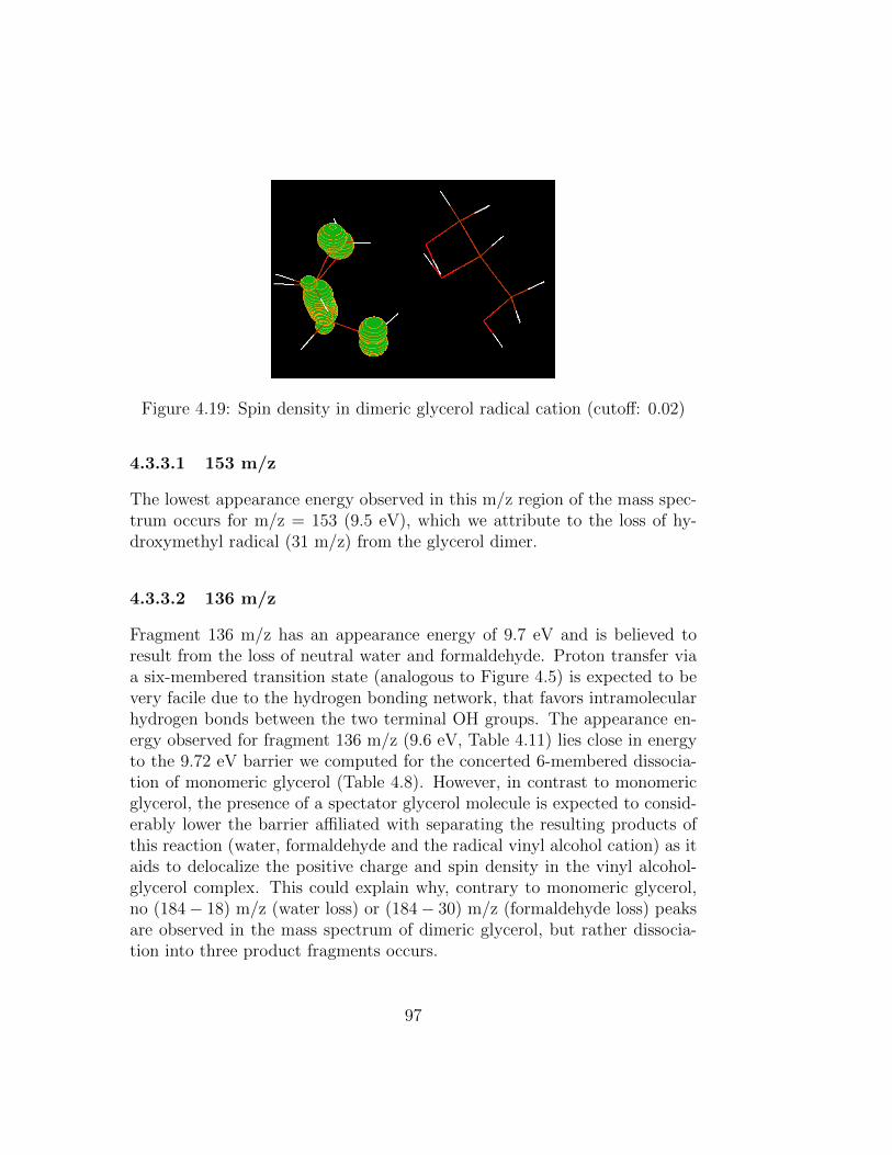
Figure 4.19: Spin density in dimeric glycerol radical cation (cutoff: 0.02)
4.3.3.1 153 m/z
The lowest appearance energy observed in this m/z region of the mass spec-trum occurs for m/z = 153 (9.5 eV), which we attribute to the loss of hy-droxymethyl radical (31 m/z) from the glycerol dimer.
4.3.3.2 136 m/z
Fragment 136 m/z has an appearance energy of 9.7 eV and is believed toresult from the loss of neutral water and formaldehyde. Proton transfer viaa six-membered transition state (analogous to Figure 4.5) is expected to bevery facile due to the hydrogen bonding network, that favors intramolecularhydrogen bonds between the two terminal OH groups. The appearance en-ergy observed for fragment 136 m/z (9.6 eV, Table 4.11) lies close in energyto the 9.72 eV barrier we computed for the concerted 6-membered dissocia-tion of monomeric glycerol (Table 4.8). However, in contrast to monomericglycerol, the presence of a spectator glycerol molecule is expected to consid-erably lower the barrier affiliated with separating the resulting products ofthis reaction (water, formaldehyde and the radical vinyl alcohol cation) as itaids to delocalize the positive charge and spin density in the vinyl alcohol-glycerol complex. This could explain why, contrary to monomeric glycerol,no (184− 18) m/z (water loss) or (184− 30) m/z (formaldehyde loss) peaksare observed in the mass spectrum of dimeric glycerol, but rather dissocia-tion into three product fragments occurs.
97

4.3.3.3 93 m/z and 185 m/z
93 m/z and 185 m/z correspond to protonated monomeric and dimeric glyc-erol, respectively. As was shown in a previous section (4.3.2.3) uptake of ahydrogen radical is energetically very favorable, but not observed until muchhigher energies experimentally (Table 4.11). We propose that the protonatedspecies occur from H• transfer between (glycerol)2 and (glycerol)3, respec-tively, followed by dissociation of the cluster into fragments, as follows:
[gly2]+• → [gly −H]• + [gly +H]+ (4.2)
[gly3]+• → [gly −H]• + [gly2 +H]+ (4.3)
The m/z = 91 species, [gly - H]•, is not detected in the mass spectrumas it is not charged. Although such a process is highly unlikely in a non-radicaloid species (c.f. the pKa value of an OH group in glycerol), ionizationmakes this process feasible. The products for reaction 4.2, for example, lieat 9.56 eV (ωB97X/6-311++G(p,d)//B3LYP/6-311++G(p,d)) with respectto two neutral isolated glycerol molecules (conformer 100).
4.4 Conclusions
In this study the dissociative photoionizations of glycerol and glycerol dimerwere investigated both experimentally and theoretically. Low pressure con-ditions combined with tunable synchrotron radiation and time-of-flight massspectrometry allowed appearance energies of radicaloid species to be deter-mined with high-energy resolution. Glycerol was found to have a very highaffinity to fragment upon photoionization, which we propose to be due tothe extremely weakened carbon framework in the glycerol radical cation.Just above the ionization potential, water- and formaldehyde loss fragmentswere observed. Computations revealed that a six-membered transition state,leading to a product complex composed of formaldehyde, water and vinylalcohol radical, is involved in this process. Separation of the three productsin monomeric glycerol is energetically unfavorable and explains why the ap-pearance of either water or formaldehyde products is observed first. We alsoelucidated detailed mechanisms leading to fragments which are observed athigher energies, such as the loss of methanol and hydroxymethyl radical, as
98
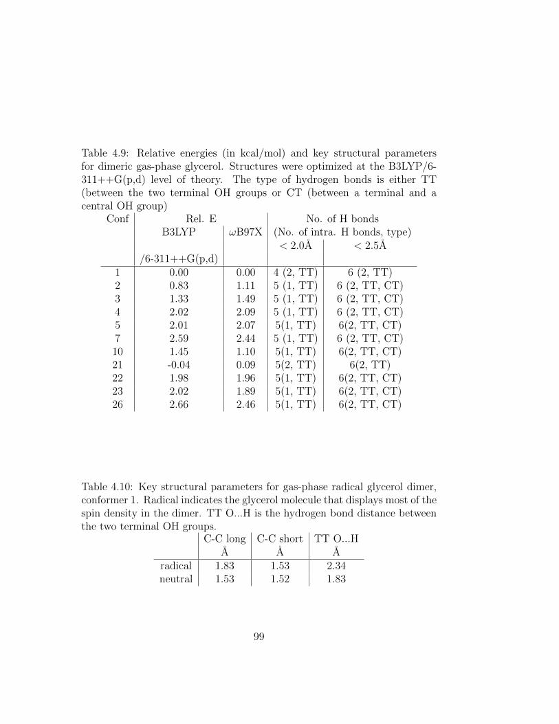
Table 4.9: Relative energies (in kcal/mol) and key structural parametersfor dimeric gas-phase glycerol. Structures were optimized at the B3LYP/6-311++G(p,d) level of theory. The type of hydrogen bonds is either TT(between the two terminal OH groups or CT (between a terminal and acentral OH group)
Conf Rel. E No. of H bondsB3LYP ωB97X (No. of intra. H bonds, type)
< 2.0A < 2.5A/6-311++G(p,d)
1 0.00 0.00 4 (2, TT) 6 (2, TT)2 0.83 1.11 5 (1, TT) 6 (2, TT, CT)3 1.33 1.49 5 (1, TT) 6 (2, TT, CT)4 2.02 2.09 5 (1, TT) 6 (2, TT, CT)5 2.01 2.07 5(1, TT) 6(2, TT, CT)7 2.59 2.44 5 (1, TT) 6 (2, TT, CT)10 1.45 1.10 5(1, TT) 6(2, TT, CT)21 -0.04 0.09 5(2, TT) 6(2, TT)22 1.98 1.96 5(1, TT) 6(2, TT, CT)23 2.02 1.89 5(1, TT) 6(2, TT, CT)26 2.66 2.46 5(1, TT) 6(2, TT, CT)
Table 4.10: Key structural parameters for gas-phase radical glycerol dimer,conformer 1. Radical indicates the glycerol molecule that displays most of thespin density in the dimer. TT O...H is the hydrogen bond distance betweenthe two terminal OH groups.
C-C long C-C short TT O...HA A A
radical 1.83 1.53 2.34neutral 1.53 1.52 1.83
99
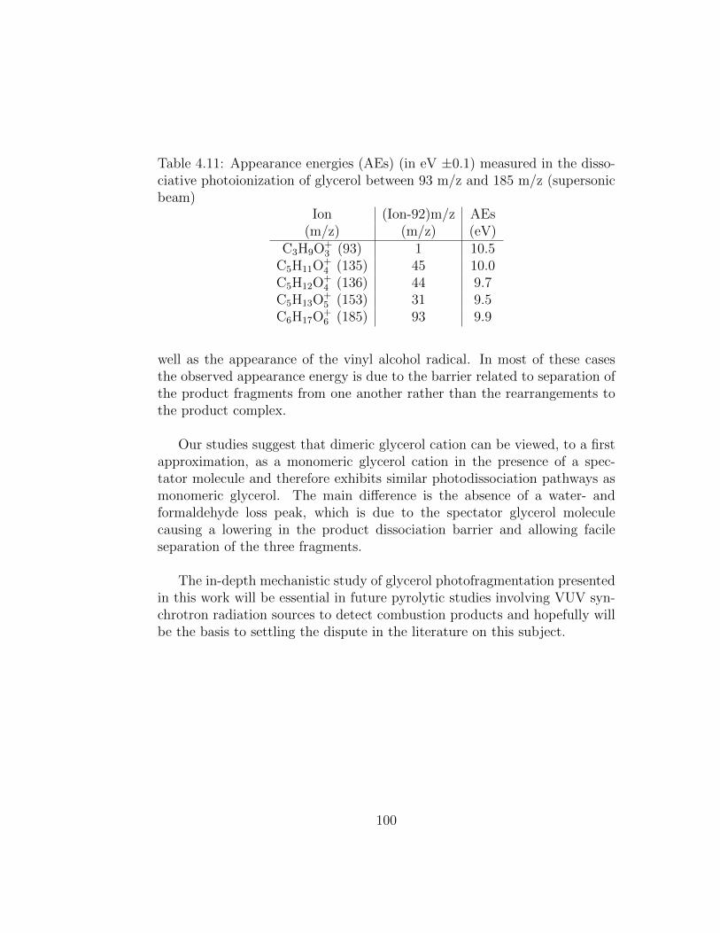
Table 4.11: Appearance energies (AEs) (in eV ±0.1) measured in the disso-ciative photoionization of glycerol between 93 m/z and 185 m/z (supersonicbeam)
Ion (Ion-92)m/z AEs(m/z) (m/z) (eV)
C3H9O+3 (93) 1 10.5
C5H11O+4 (135) 45 10.0
C5H12O+4 (136) 44 9.7
C5H13O+5 (153) 31 9.5
C6H17O+6 (185) 93 9.9
well as the appearance of the vinyl alcohol radical. In most of these casesthe observed appearance energy is due to the barrier related to separation ofthe product fragments from one another rather than the rearrangements tothe product complex.
Our studies suggest that dimeric glycerol cation can be viewed, to a firstapproximation, as a monomeric glycerol cation in the presence of a spec-tator molecule and therefore exhibits similar photodissociation pathways asmonomeric glycerol. The main difference is the absence of a water- andformaldehyde loss peak, which is due to the spectator glycerol moleculecausing a lowering in the product dissociation barrier and allowing facileseparation of the three fragments.
The in-depth mechanistic study of glycerol photofragmentation presentedin this work will be essential in future pyrolytic studies involving VUV syn-chrotron radiation sources to detect combustion products and hopefully willbe the basis to settling the dispute in the literature on this subject.
100
Chapter 5
Theoretical study ofsubstituted PBPB dimers:Structural analysis, tetraradicalcharacter and excited states
The radicaloid nature of para and meta 1,3-diborata-2,4-diphosphoniocyclo-butane-1,3-diyl doubly substituted benzene is assessed from several electronicstructure perspectives. Orbital occupation numbers computed by perfectpairing (PP), complete active space SCF (CASSCF) and restricted activespace double spin-flip (RAS-2SF) reveal the presence of less than one un-paired electron in the planar molecules. Thus, the surprising stability ofthe para tetraradical, can be rationalized by its moderate extent of radicalcharacter. Estimation of the delocalization energy, low-lying excited statesand short and long range magnetic coupling constants, all indicate a ratherweak interaction to occur between two singlet PBPB units. Communicationbetween two triplet units was found to be negligible. Comparison betweenpara and meta isomers confirms a distinctly larger communication via theframework for the former. However, this communication, which was recentlyproposed to be the main factor for the different behavior of meta and paraisomers regarding their preferred geometries, was found to account for onlyone third of their energy difference. The study shows the important contribu-tion of steric and/or electronic effects of the bulky iPr and tBu substituentson P and B.
101

5.1 Introduction
In search for molecular materials with new interesting properties, main groupelement radicaloid systems have become an intensively studied topic in thepast and recent years [333–336]. Among them, diradicals are molecules fea-turing two unpaired electrons, each of which is occupying two degenerateor nearly degenerate molecular orbitals (MOs) [337–340]. Due to the un-paired nature of these systems, diradicals are usually very reactive [340,341]and thus short-lived. The linkage of two or more radical moieties appearsto be one of the most successful and extensively studied strategies to yieldmolecules of polyradicaloid character. Moreover, this procedure allows theachievement of different electronic properties by modifying the nature of thelinker practically at will [342,343].
Particularly interesting is the catenation of singlet diradical monomers,which is predicted to yield antiferromagnetic low-spin polymers [344, 345].Their half-filled electron bands would confer the capability for metallic con-duction without doping [341,346–349]. In this direction, several carbon baseddi- [350] and tetraradical [342, 351–357] prototypes have been prepared, buttheir extremely short half-life constitutes a major drawback. However, re-cently, a few stable diradicals based on main-group elements have been iso-lated [358–367]. Amongst them, 1,3-diborata-2,4-diphosphoniocyclobutane-1,3-diyls (1A in Figure 5.1), yield a localized singlet diradical that is in-definitely stable at room temperature on adequate choice of substituents[368]. Thus these systems are one of the currently most promising buildingblocks for low-spin polymers. This made them subject to several experimen-tal [369,370] as well as theoretical studies [371–375].
Recently, Rodriguez et. al. catenated two of these moieties successfullyvia para and meta-phenylene linkers [376]. Experimental data in solid stateas well as in solution of these new compounds indicates that the topologyof the linker plays a crucial role in their structural and electronic properties.X-ray diffraction analysis reveals that the para isomer exhibits virtually pla-nar PBPB moieties, which are coplanar to the phenyl ring (p-3A in Figure5.1), and was proposed to be the first stable singlet tetraradical [376]. Onthe other hand, the meta-phenylene linker favors a bis(bicycle) arrangement(m-3B in Figure 5.1) and the system does not feature any radicaloid charac-
102
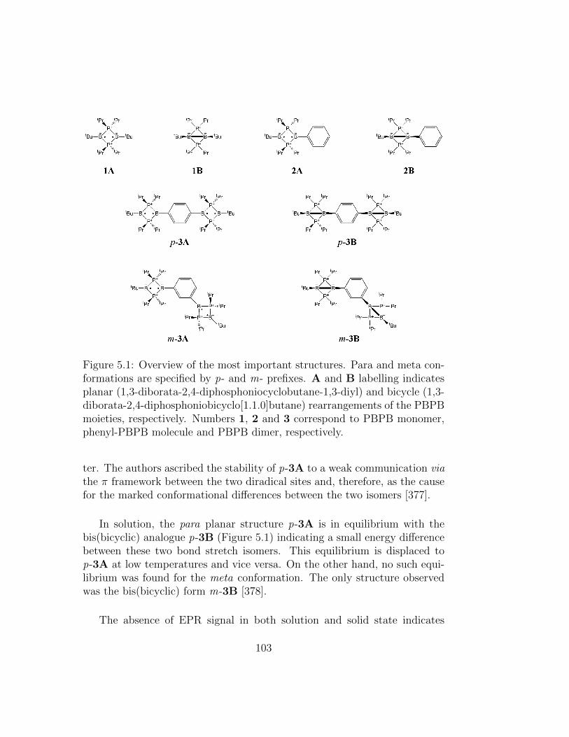
Figure 5.1: Overview of the most important structures. Para and meta con-formations are specified by p- and m- prefixes. A and B labelling indicatesplanar (1,3-diborata-2,4-diphosphoniocyclobutane-1,3-diyl) and bicycle (1,3-diborata-2,4-diphosphoniobicyclo[1.1.0]butane) rearrangements of the PBPBmoieties, respectively. Numbers 1, 2 and 3 correspond to PBPB monomer,phenyl-PBPB molecule and PBPB dimer, respectively.
ter. The authors ascribed the stability of p-3A to a weak communication viathe π framework between the two diradical sites and, therefore, as the causefor the marked conformational differences between the two isomers [377].
In solution, the para planar structure p-3A is in equilibrium with thebis(bicyclic) analogue p-3B (Figure 5.1) indicating a small energy differencebetween these two bond stretch isomers. This equilibrium is displaced top-3A at low temperatures and vice versa. On the other hand, no such equi-librium was found for the meta conformation. The only structure observedwas the bis(bicyclic) form m-3B [378].
The absence of EPR signal in both solution and solid state indicates
103
that p-3A features a singlet ground state, but the absence of an EPR sig-nal is not definitive. Hence, the ground state multiplicity of the systemsneeds to be confirmed. Moreover, although p-3A was predicted to exhibittetradicaloid character, its extent has not yet been quantified. The radicalcharacter concept is mainly based on chemical intuition, as there is no quan-tum mechanical operator that defines the extent of pairing unambiguously.Consequently, there can be no direct measurement of radical character.
Although experimental efforts and preliminary computational analysishave provided a better understanding of these systems, several questions stillremain open for a full comprehension: Can calculations confirm the presenceof a π interaction between the two PBPB units in the para compound p-3A?Is this interaction the sole reason for the geometrical differences observedbetween meta and para isomers? Is the electronic ground state of p-3A asinglet? What is the extent of its tetraradical character?
This work comes to answer these and other related questions for thepara-phenylene and meta-phenylene linkage of two PBPB skeletons. Thepresent study is organized as follows: first, we detail the computational toolsemployed. Then, we discuss the main structural characteristics, the stabilityof the different species, and the tetraradical nature and magnetic couplingsof planar systems. Finally, the main conclusions will be outlined.
5.2 Computational Details
Molecular geometry optimizations and frequency analysis were performedat the B3LYP level in combination with the 6-31G(d) basis set [379]. Theadequacy of the 6-31G(d) basis set was tested against the much larger 6-311G(3df,2pd) basis [380,381] for the H-substituted molecular models (see be-low), and hardly any effect on the optimized geometries was observed. The 6-31G(d) basis set was also employed in all other electronic structure computa-tions. Relative energy stability between bond-strech and meta/para isomerswas explored by B3LYP and the resolution-of-identity (RI) [159, 382–384]implementation [385,386] of the coupled-cluster (CC) formulation of perfectpairing (PP) [79,387]. The VDZ auxiliary basis [388] for RI-MP2 was chosenin the RI approach. The tetraradicaloid character of planar molecules wasdetermined through the orbital occupation numbers from the one particle
104

density matrix of PP, complete active space SCF (CASSCF) [389] with 4 or-bitals and 4 electrons in the active space and the restricted active space dou-ble spin-flip (RAS-2SF) method [3], and by means of the perfect quadruples(PQ) [81], CASSCF(4,4) and RAS-2SF single amplitudes of the T4 clusteroperator. All RAS-2SF calculations were performed within the (hole, parti-cle) truncation and using a restricted open shell (ROHF) high spin quintetas reference to obtain MS = 0 states. In order to understand the role of thesubstituent groups in phosphorus and boron atoms, and for the sake of lowercomputational cost as well, calculations were also carried out on model sys-tems, in which hydrogen atoms have replaced the tBu and iPr groups. Thesemolecules will be labeled analogously to their parent compounds (see Figure5.1), but with an H at the end. Since all H-substituted model systems featurethe bis(bicyclic) geometry as their ground state, optimizations of the planarconformations were carried out by restricting the geometry optimization tothe corresponding symmetry point group. Most of the calculations were per-formed using a development version of the Q-CHEM package [311]. Completeactive space SCF was carried out with the 2009 version of GAMESS [390].
5.3 Results and Discussion
In this section the most relevant aspects related to geometries, energies, thecommunication and magnetic coupling between PBPB moieties, and the low-lying states of the planar molecules, will be discussed.
5.3.1 Molecular Geometries
First of all, we perform a structural analysis of the 1, 2 and 3 compounds forthe different conformations and substitutions. The most relevant computa-tionally optimized and experimental bond distances and the BPPB dihedralangle are shown in Tables 7.1-5.3.
The structural parameters of the optimized PBPB unit in the planar con-formation, 1A, are in very good agreement with X-ray experimental data insolid state [368, 369](7.1). The optimized geometry of 1A is also very closeto previous calculations by Scheschkewitz et. al. [368] at similar level of the-ory. The main difference lies in the interflap angle between the two PBPBunits. Whereas an angle of 180◦ was found in this study, Scheschkewitz’sresult indicate 174◦. Comparison between 1A and the H-substituted (1AH)
105

Figure 5.2: Atomic labeling of PBPB used in the description of geometricalparameters (Tables 7.1-5.3). Although the B-B bond is not represented,labels are applicable for both, planar (A) and bicyclic (B) molecules.
system reveals one important difference. Replacing the iPr and tBu groupsby hydrogen atoms at P and B, respectively, transforms the planar structurefrom minimum of the potential energy surface into first order saddle point,which has been already observed [368]. The associated imaginary frequencycorresponds to the B-B bond formation process. Besides this, only slightdifferences between optimized and experimental 1A, and the H-substitutedplanar PBPB core geometries were obtained. Differences in the atomic dis-tances are never larger than 0.03 A (B · · · B in 1A /1 AH).
The H-substituted monomeric bicyclic compound, 1BH, features a sub-stantially shortened B-B bond length compared to the substituted analogue,1B (Table 5.2). This contraction is a result of the lack of steric hindrancein 1BH, which allows the two boron atoms to approach more closely. Thisis accompanied by a much smaller BPPB dihedral angle in 1BH (δ = 92◦)than in the fully substituted analog (δ = 141◦).
Optimized structural parameters of p-3A (and p-3AH) are very closeto experimental data [376]. Analogously to 1AH, the planar p-3AH andm-3AH molecules are now second order saddle points, with two imaginaryfrequencies corresponding to B-B bond formation. The main bond distancedifference between p-3A and m-3A corresponds to B-CPh, which is less than0.015 A larger in the meta substitution. Again, there is a good agreementbetween computed and experimental m-3B geometries. The most significantdifference between p-3B and m-3B is the B-B bond distance, being ∼ 0.02A larger in the meta isomer. The p-3BH and m-3BH modeled structurespresent shorter B-B bond distances by 0.05 and 0.07 A, respectively, thanthe fully substituted molecules. Dihedral angles (δ in Tables 7.1 and 5.2)are considerably smaller in the model systems. Optimized 2A and 2B (andtheir hydrogen analogues) do not present any significant particularity with
106
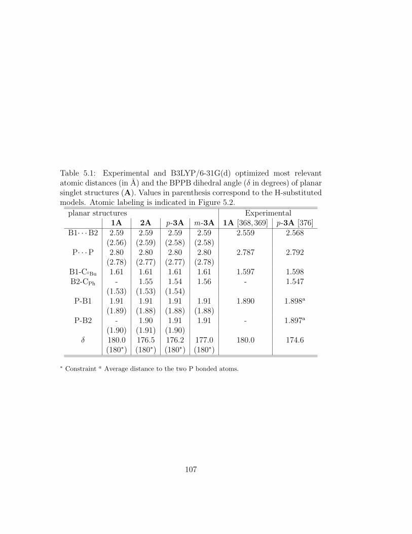
Table 5.1: Experimental and B3LYP/6-31G(d) optimized most relevantatomic distances (in A) and the BPPB dihedral angle (δ in degrees) of planarsinglet structures (A). Values in parenthesis correspond to the H-substitutedmodels. Atomic labeling is indicated in Figure 5.2.
planar structures Experimental1A 2A p-3A m-3A 1A [368,369] p-3A [376]
B1· · ·B2 2.59 2.59 2.59 2.59 2.559 2.568(2.56) (2.59) (2.58) (2.58)
P· · ·P 2.80 2.80 2.80 2.80 2.787 2.792(2.78) (2.77) (2.77) (2.78)
B1-CtBu 1.61 1.61 1.61 1.61 1.597 1.598B2-CPh - 1.55 1.54 1.56 - 1.547
(1.53) (1.53) (1.54)P-B1 1.91 1.91 1.91 1.91 1.890 1.898a
(1.89) (1.88) (1.88) (1.88)P-B2 - 1.90 1.91 1.91 - 1.897a
(1.90) (1.91) (1.90)δ 180.0 176.5 176.2 177.0 180.0 174.6
(180∗) (180∗) (180∗) (180∗)
∗ Constraint a Average distance to the two P bonded atoms.
107
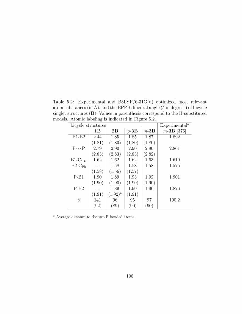
Table 5.2: Experimental and B3LYP/6-31G(d) optimized most relevantatomic distances (in A), and the BPPB dihedral angle (δ in degrees) of bicyclesinglet structures (B). Values in parenthesis correspond to the H-substitutedmodels. Atomic labeling is indicated in Figure 5.2.
bicycle structures Experimentala
1B 2B p-3B m-3B m-3B [376]B1-B2 2.44 1.85 1.85 1.87 1.892
(1.81) (1.80) (1.80) (1.80)P· · ·P 2.79 2.90 2.90 2.90 2.861
(2.83) (2.83) (2.83) (2.82)B1-CtBu 1.62 1.62 1.62 1.63 1.610B2-CPh - 1.58 1.58 1.58 1.575
(1.58) (1.56) (1.57)P-B1 1.90 1.89 1.93 1.92 1.901
(1.90) (1.90) (1.90) (1.90)P-B2 - 1.89 1.90 1.90 1.876
(1.91) (1.92)a (1.91)δ 141 96 95 97 100.2
(92) (89) (90) (90)
a Average distance to the two P bonded atoms.
108
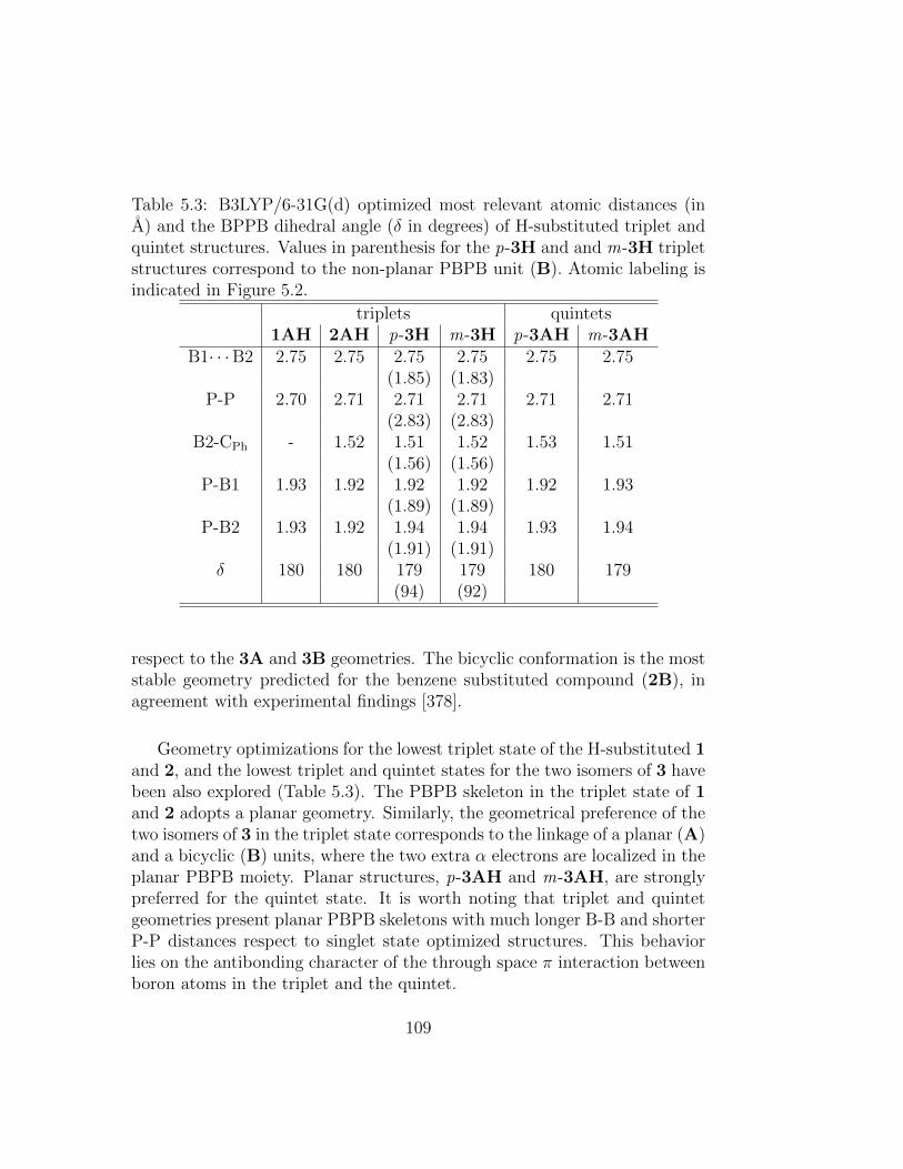
Table 5.3: B3LYP/6-31G(d) optimized most relevant atomic distances (inA) and the BPPB dihedral angle (δ in degrees) of H-substituted triplet andquintet structures. Values in parenthesis for the p-3H and and m-3H tripletstructures correspond to the non-planar PBPB unit (B). Atomic labeling isindicated in Figure 5.2.
triplets quintets1AH 2AH p-3H m-3H p-3AH m-3AH
B1· · ·B2 2.75 2.75 2.75 2.75 2.75 2.75(1.85) (1.83)
P-P 2.70 2.71 2.71 2.71 2.71 2.71(2.83) (2.83)
B2-CPh - 1.52 1.51 1.52 1.53 1.51(1.56) (1.56)
P-B1 1.93 1.92 1.92 1.92 1.92 1.93(1.89) (1.89)
P-B2 1.93 1.92 1.94 1.94 1.93 1.94(1.91) (1.91)
δ 180 180 179 179 180 179(94) (92)
respect to the 3A and 3B geometries. The bicyclic conformation is the moststable geometry predicted for the benzene substituted compound (2B), inagreement with experimental findings [378].
Geometry optimizations for the lowest triplet state of the H-substituted 1and 2, and the lowest triplet and quintet states for the two isomers of 3 havebeen also explored (Table 5.3). The PBPB skeleton in the triplet state of 1and 2 adopts a planar geometry. Similarly, the geometrical preference of thetwo isomers of 3 in the triplet state corresponds to the linkage of a planar (A)and a bicyclic (B) units, where the two extra α electrons are localized in theplanar PBPB moiety. Planar structures, p-3AH and m-3AH, are stronglypreferred for the quintet state. It is worth noting that triplet and quintetgeometries present planar PBPB skeletons with much longer B-B and shorterP-P distances respect to singlet state optimized structures. This behaviorlies on the antibonding character of the through space π interaction betweenboron atoms in the triplet and the quintet.
109
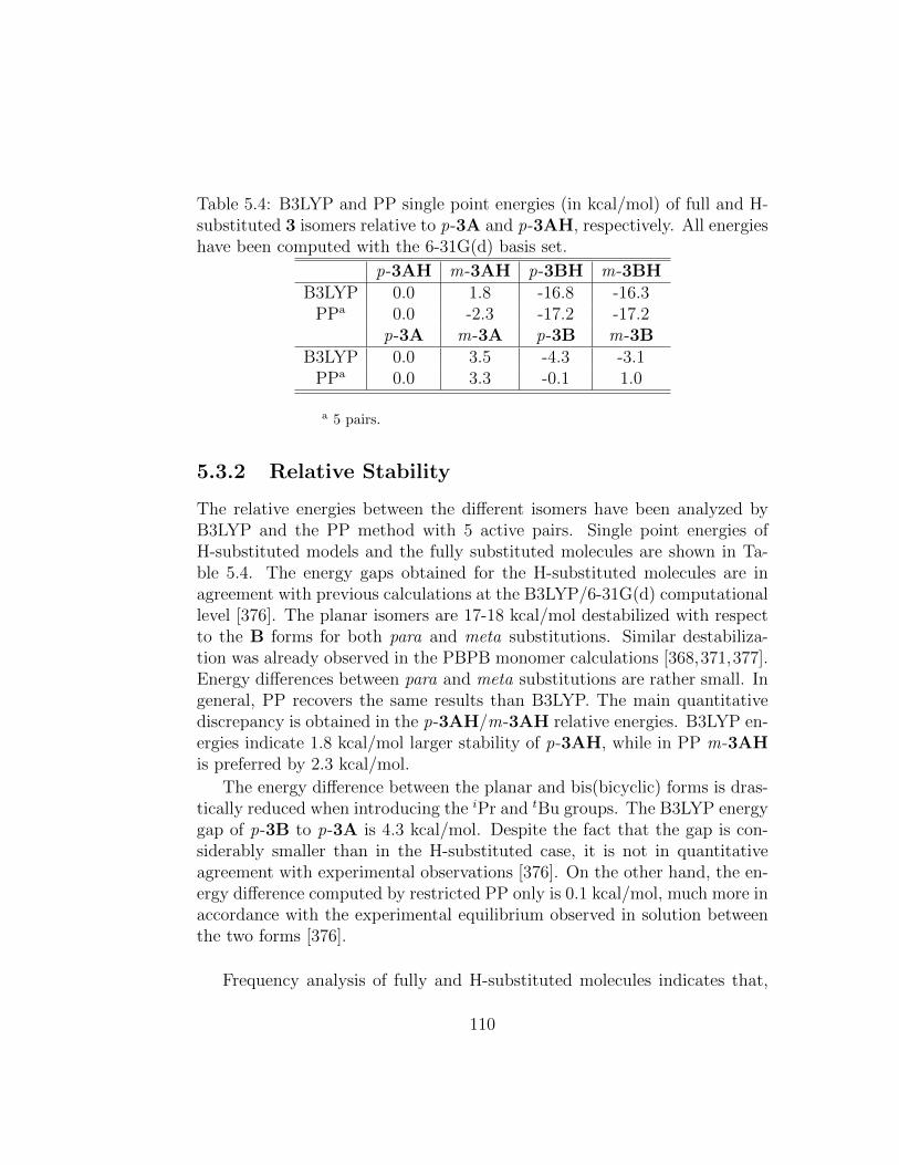
Table 5.4: B3LYP and PP single point energies (in kcal/mol) of full and H-substituted 3 isomers relative to p-3A and p-3AH, respectively. All energieshave been computed with the 6-31G(d) basis set.
p-3AH m-3AH p-3BH m-3BHB3LYP 0.0 1.8 -16.8 -16.3
PPa 0.0 -2.3 -17.2 -17.2p-3A m-3A p-3B m-3B
B3LYP 0.0 3.5 -4.3 -3.1PPa 0.0 3.3 -0.1 1.0
a 5 pairs.
5.3.2 Relative Stability
The relative energies between the different isomers have been analyzed byB3LYP and the PP method with 5 active pairs. Single point energies ofH-substituted models and the fully substituted molecules are shown in Ta-ble 5.4. The energy gaps obtained for the H-substituted molecules are inagreement with previous calculations at the B3LYP/6-31G(d) computationallevel [376]. The planar isomers are 17-18 kcal/mol destabilized with respectto the B forms for both para and meta substitutions. Similar destabiliza-tion was already observed in the PBPB monomer calculations [368,371,377].Energy differences between para and meta substitutions are rather small. Ingeneral, PP recovers the same results than B3LYP. The main quantitativediscrepancy is obtained in the p-3AH/m-3AH relative energies. B3LYP en-ergies indicate 1.8 kcal/mol larger stability of p-3AH, while in PP m-3AHis preferred by 2.3 kcal/mol.
The energy difference between the planar and bis(bicyclic) forms is dras-tically reduced when introducing the iPr and tBu groups. The B3LYP energygap of p-3B to p-3A is 4.3 kcal/mol. Despite the fact that the gap is con-siderably smaller than in the H-substituted case, it is not in quantitativeagreement with experimental observations [376]. On the other hand, the en-ergy difference computed by restricted PP only is 0.1 kcal/mol, much more inaccordance with the experimental equilibrium observed in solution betweenthe two forms [376].
Frequency analysis of fully and H-substituted molecules indicates that,
110
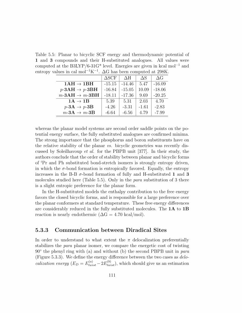
Table 5.5: Planar to bicyclic SCF energy and thermodynamic potential of1 and 3 compounds and their H-substituted analogues. All values werecomputed at the B3LYP/6-31G* level. Energies are given in kcal mol−1 andentropy values in cal mol−1K−1. ∆G has been computed at 298K.
∆SCF ∆H ∆S ∆G1AH → 1BH -15.15 -14.46 5.47 -16.09
p-3AH → p-3BH -16.84 -15.05 10.09 -18.06m-3AH → m-3BH -18.11 -17.36 9.69 -20.25
1A → 1B 5.39 5.31 2.03 4.70p-3A → p-3B -4.26 -3.31 -1.61 -2.83
m-3A → m-3B -6.64 -6.56 4.79 -7.99
whereas the planar model systems are second order saddle points on the po-tential energy surface, the fully substituted analogues are confirmed minima.The strong importance that the phosphorus and boron substituents have onthe relative stability of the planar vs. bicyclic geometries was recently dis-cussed by Soleilhavoup et al. for the PBPB unit [377]. In their study, theauthors conclude that the order of stability between planar and bicyclic formsof iPr and Ph substituted bond-stretch isomers is strongly entropy driven,in which the σ-bond formation is entropically favored. Equally, the entropyincreases in the B-B σ-bond formation of fully and H-substituted 1 and 3molecules studied here (Table 5.5). Only in the para substitution of 3 thereis a slight entropic preference for the planar form.
In the H-substituted models the enthalpy contribution to the free energyfavors the closed bicyclic forms, and is responsible for a large preference overthe planar conformers at standard temperature. These free energy differencesare considerably reduced in the fully substituted molecules. The 1A to 1Breaction is nearly endothermic (∆G = 4.70 kcal/mol).
5.3.3 Communication between Diradical Sites
In order to understand to what extent the π delocalization preferentiallystabilizes the para planar isomer, we compare the energetic cost of twisting90◦ the phenyl ring with (a) and without (b) the second PBPB unit in para(Figure 5.3.3). We define the energy difference between the two cases as delo-
calization energy (ED = E(a)twist−2E
(b)twist), which should give us an estimation
111

of the communication between the two diradical sites through the π system.
Figure 5.3: Delocalization energy in para isomers. Delocalization energyis defined as the difference between the energy cost of twisting the phenylring (a) and two times the twisting energy without one of the PBPB units(b). The same scheme is applied for fully (p-1A, R = iPr, R = tBu) andH-substituted (p-1AH, R, R = H) molecules.
The delocalization energy obtained for p-3AH (ED = 1.6 kcal/mol) co-incides well with the computed energy difference to m-3AH (1.8 kcal/mol inTable 5.4). Thus, it indicates that in the H-substituted case, the communi-cation through π framework is the main driving force of the para versus metastabilization, as it has been previously suggested [378]. The same analysison the fully substituted system yields to a very similar delocalization energy(ED = 1.4 kcal/mol), but now ED only corresponds to one third of the en-ergy gap between p-3A and m-3A (Table 5.4). One possible reason for theincreased gap could be the 10◦ and 4◦ deviation of coplanarity by the PBPBgroups in m-3A, not present in p-3A (CCBP dihedral: ∼ 3◦). However,setting the dihedral angles in m-3AH to −10◦ and −4◦ only yields a tinyenergy increase (∼ 0.1 kcal/mol) which cannot account for the remaining2.8 kcal/mol. These results suggest that steric and/or electronic factors dueto the presence of iPr and tBu groups are responsible for the remaining twothirds of the para to meta energy gap of 3A. Indeed, m-3A exhibits muchlarger steric hindrance than p-3A. Although both substitutions contain twonon-bonded hydrogen distances between one of the iPr groups and the pheny-lene linker which fall within the van der Waals range (2.18-2.40 A) [391,392]these are ∼ 0.1 A shorter in the meta isomer, i.e. 2.17-2.21 A and 2.28-2.29
112
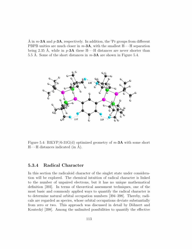
A in m-3A and p-3A, respectively. In addition, the iPr groups from differentPBPB unities are much closer in m-3A, with the smallest H· · ·H separationbeing 2.35 A, while in p-3A these H· · ·H distances are never shorter than5.5 A. Some of the short distances in m-3A are shown in Figure 5.4.
Figure 5.4: B3LYP/6-31G(d) optimized geometry of m-3A with some shortH· · ·H distances indicated (in A).
5.3.4 Radical Character
In this section the radicaloid character of the singlet state under considera-tion will be explored. The chemical intuition of radical character is linkedto the number of unpaired electrons, but it has no unique mathematicaldefinition [393]. In terms of theoretical assessment techniques, one of themost basic and commonly applied ways to quantify the radical character isto determine natural orbital occupation numbers [394–398]. Thereby, radi-cals are regarded as species, whose orbital occupations deviate substantiallyfrom zero or two. This approach was discussed in detail by Dohnert andKoutecky [398]. Among the unlimited possibilities to quantify the effective
113
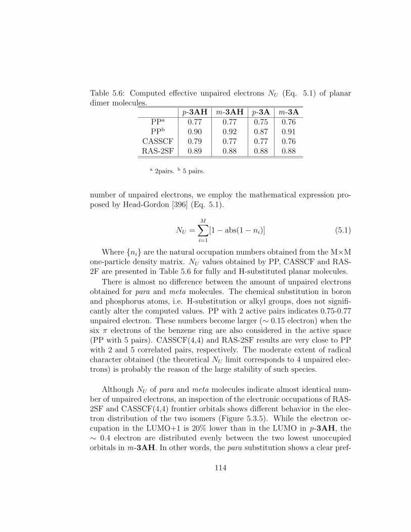
Table 5.6: Computed effective unpaired electrons NU (Eq. 5.1) of planardimer molecules.
p-3AH m-3AH p-3A m-3APPa 0.77 0.77 0.75 0.76PPb 0.90 0.92 0.87 0.91
CASSCF 0.79 0.77 0.77 0.76RAS-2SF 0.89 0.88 0.88 0.88
a 2pairs. b 5 pairs.
number of unpaired electrons, we employ the mathematical expression pro-posed by Head-Gordon [396] (Eq. 5.1).
NU =M∑i=1
[1− abs(1− ni)] (5.1)
Where {ni} are the natural occupation numbers obtained from the M×Mone-particle density matrix. NU values obtained by PP, CASSCF and RAS-2F are presented in Table 5.6 for fully and H-substituted planar molecules.
There is almost no difference between the amount of unpaired electronsobtained for para and meta molecules. The chemical substitution in boronand phosphorus atoms, i.e. H-substitution or alkyl groups, does not signifi-cantly alter the computed values. PP with 2 active pairs indicates 0.75-0.77unpaired electron. These numbers become larger (∼ 0.15 electron) when thesix π electrons of the benzene ring are also considered in the active space(PP with 5 pairs). CASSCF(4,4) and RAS-2SF results are very close to PPwith 2 and 5 correlated pairs, respectively. The moderate extent of radicalcharacter obtained (the theoretical NU limit corresponds to 4 unpaired elec-trons) is probably the reason of the large stability of such species.
Although NU of para and meta molecules indicate almost identical num-ber of unpaired electrons, an inspection of the electronic occupations of RAS-2SF and CASSCF(4,4) frontier orbitals shows different behavior in the elec-tron distribution of the two isomers (Figure 5.3.5). While the electron oc-cupation in the LUMO+1 is 20% lower than in the LUMO in p-3AH, the∼ 0.4 electron are distributed evenly between the two lowest unoccupiedorbitals in m-3AH. In other words, the para substitution shows a clear pref-
114

erence for the π-bonding interaction between the two molecular ends, while π-bonding/π-antibonding interactions through the phenylene linker are hardlydistinguished in m-3AH. A similar analysis can be done from the HOMOand HOMO-1 occupations.
At this point, we have analyzed the radical character by means of theeffective unpaired electrons (Eq. 5.1), but we still must face the question towhich extent the singlet ground state of p-3A and m-3A should be consideredtetraradicaloids. One possibility to quantify this property is by extending theelectronic structure properties of a singlet diradicaloid to a tetraradicaloidspecies, e.g. the extent of open shell singlet character. For a system featuringfour unpaired electrons, an open shell singlet can be achieved by coupling twosinglet or two triplet units, respectively. The former can be interpreted as acommunication between two singlet diradical sites. The latter constitutes anovel configuration, which corresponds to the concomitant excitation of thetwo sub-units, and could be used to discern between two interacting diradicalmoieties (two sets of two strongly correlated electrons) and a true tetraradical(four strongly correlated electrons).
115
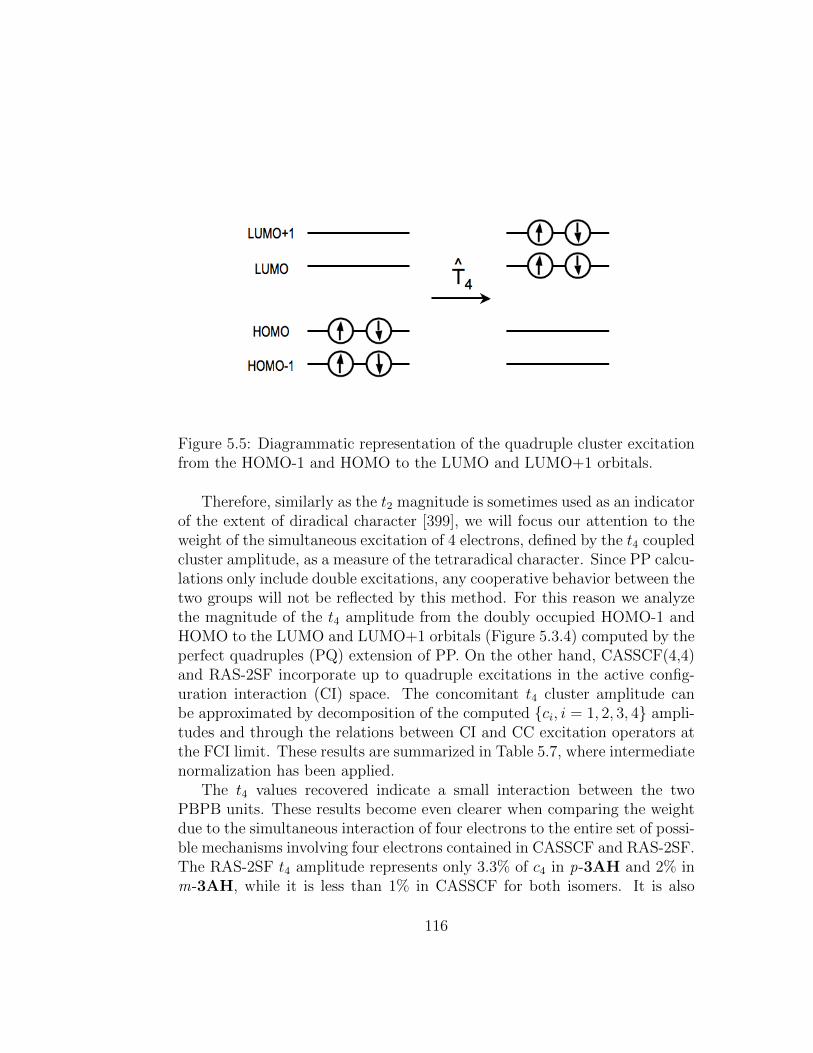
Figure 5.5: Diagrammatic representation of the quadruple cluster excitationfrom the HOMO-1 and HOMO to the LUMO and LUMO+1 orbitals.
Therefore, similarly as the t2 magnitude is sometimes used as an indicatorof the extent of diradical character [399], we will focus our attention to theweight of the simultaneous excitation of 4 electrons, defined by the t4 coupledcluster amplitude, as a measure of the tetraradical character. Since PP calcu-lations only include double excitations, any cooperative behavior between thetwo groups will not be reflected by this method. For this reason we analyzethe magnitude of the t4 amplitude from the doubly occupied HOMO-1 andHOMO to the LUMO and LUMO+1 orbitals (Figure 5.3.4) computed by theperfect quadruples (PQ) extension of PP. On the other hand, CASSCF(4,4)and RAS-2SF incorporate up to quadruple excitations in the active config-uration interaction (CI) space. The concomitant t4 cluster amplitude canbe approximated by decomposition of the computed {ci, i = 1, 2, 3, 4} ampli-tudes and through the relations between CI and CC excitation operators atthe FCI limit. These results are summarized in Table 5.7, where intermediatenormalization has been applied.
The t4 values recovered indicate a small interaction between the twoPBPB units. These results become even clearer when comparing the weightdue to the simultaneous interaction of four electrons to the entire set of possi-ble mechanisms involving four electrons contained in CASSCF and RAS-2SF.The RAS-2SF t4 amplitude represents only 3.3% of c4 in p-3AH and 2% inm-3AH, while it is less than 1% in CASSCF for both isomers. It is also
116
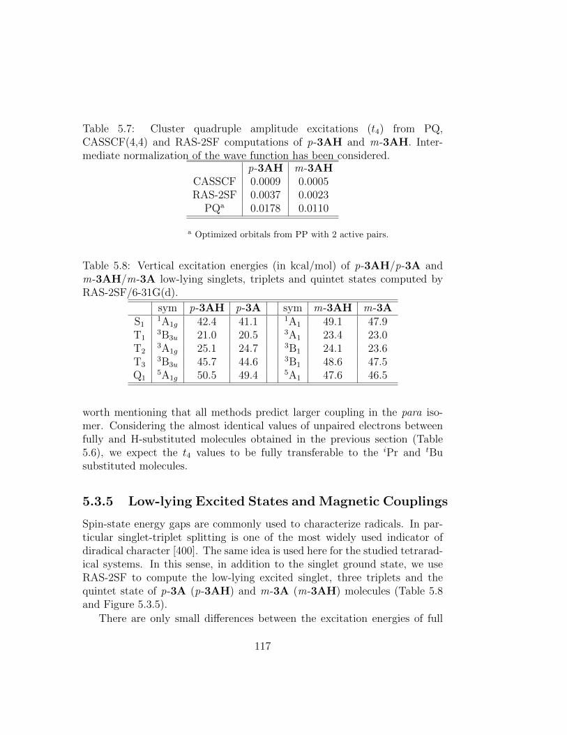
Table 5.7: Cluster quadruple amplitude excitations (t4) from PQ,CASSCF(4,4) and RAS-2SF computations of p-3AH and m-3AH. Inter-mediate normalization of the wave function has been considered.
p-3AH m-3AHCASSCF 0.0009 0.0005RAS-2SF 0.0037 0.0023
PQa 0.0178 0.0110
a Optimized orbitals from PP with 2 active pairs.
Table 5.8: Vertical excitation energies (in kcal/mol) of p-3AH/p-3A andm-3AH/m-3A low-lying singlets, triplets and quintet states computed byRAS-2SF/6-31G(d).
sym p-3AH p-3A sym m-3AH m-3AS1
1A1g 42.4 41.1 1A1 49.1 47.9T1
3B3u 21.0 20.5 3A1 23.4 23.0T2
3A1g 25.1 24.7 3B1 24.1 23.6T3
3B3u 45.7 44.6 3B1 48.6 47.5Q1
5A1g 50.5 49.4 5A1 47.6 46.5
worth mentioning that all methods predict larger coupling in the para iso-mer. Considering the almost identical values of unpaired electrons betweenfully and H-substituted molecules obtained in the previous section (Table5.6), we expect the t4 values to be fully transferable to the iPr and tBusubstituted molecules.
5.3.5 Low-lying Excited States and Magnetic Couplings
Spin-state energy gaps are commonly used to characterize radicals. In par-ticular singlet-triplet splitting is one of the most widely used indicator ofdiradical character [400]. The same idea is used here for the studied tetrarad-ical systems. In this sense, in addition to the singlet ground state, we useRAS-2SF to compute the low-lying excited singlet, three triplets and thequintet state of p-3A (p-3AH) and m-3A (m-3AH) molecules (Table 5.8and Figure 5.3.5).
There are only small differences between the excitation energies of full
117
and H-substituted molecules. When alkyl groups are taken into account theexcitation energies are slightly reduced by 0.4-1.2 kcal/mol. The two lowesttriplets, e.g. T1 and T2, lie 20-25 kcal/mol above the singlet ground state inboth isomers, but in p-3A (p-3AH) the energy separation between 3B3u and3A1g is close to 4 kcal/mol, while in m-3A (m-3AH) the two triplets, 3A1
and 3B1, are only 0.6 kcal/mol apart. The para and meta highest tripletscorrespond to doubly excited configurations with B3u and B1 symmetries,respectively. The first excited singlet state (S1) is mainly built up fromsimilar contributions of doubly excited closed shell configurations from theclosed shell single determinant (Hartree Fock like) ground state. Finally, theMS = 0 quintet state is obtained as the totally symmetric combination of 4unpaired electrons in the 4 frontier orbitals (Figure 5.3.5).
Despite the lack of dynamical correlation in RAS-2SF, it is been shown[401] that the balanced treatment of low-lying states of radicaloid systemsmakes it very suitable in the computation of energy gaps. At the same time,the reader should be rather cautious in taking the results presented above asa benchmark for the vertical transitions of p-3A and m-3A.
5.3.6 Magnetic Couplings
Some of the features of para and meta PBPB dimers computed vertical exci-tation energies can be rationalized through the phenomenological HeisenbergHamiltonian (Eq. 5.2) that describes the exchange interaction between para-magnetic centers.
H = −∑i<j
JijSiSj (5.2)
Where Si and Sj are the total spins in each paramagnetic center, and J isknown as the exchange constant [402]. Positive J values indicate ferromag-netic interaction (parallel spins), while negative values correspond to antifer-romagnetic coupling (antiparallel spins). The application of the Heisenbergmodel to p-3A (p-3AH) and m-3A (m-3AH) can be used to describe theinteraction between the four boron atoms (S = 1/2). As a simple approxima-tion of the four-center problem, we only take two kinds of magnetic couplingsinto account: the short range interactions (σ) between the two boron atomsin the same PBPB skeleton and a long range interaction (λ) through thephenylene linker (centers 2 and 3 in Figure 5.3.6), i.e. only interactions
118
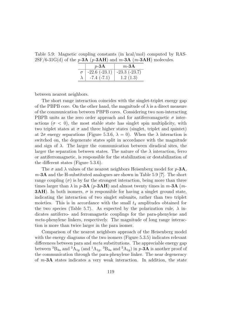
Table 5.9: Magnetic coupling constants (in kcal/mol) computed by RAS-2SF/6-31G(d) of the p-3A (p-3AH) and m-3A (m-3AH) molecules.
p-3A m-3Aσ -22.6 (-23.1) -23.3 (-23.7)λ -7.4 (-7.1) 1.2 (1.3)
between nearest neighbors.
The short range interaction coincides with the singlet-triplet energy gapof the PBPB core. On the other hand, the magnitude of λ is a direct measureof the communication between PBPB cores. Considering two non-interactingPBPB units as the zero order approach and for antiferromagnetic σ inter-actions (σ < 0), the most stable state has singlet spin multiplicity, withtwo triplet states at σ and three higher states (singlet, triplet and quintet)at 2σ energy separations (Figure 5.3.6, λ = 0). When the λ interaction isswitched on, the degenerate states split in accordance with the magnitudeand sign of λ. The larger the communication between diradical sites, thelarger the separation between states. The nature of the λ interaction, ferroor antiferromagnetic, is responsible for the stabilization or destabilization ofthe different states (Figure 5.3.6).
The σ and λ values of the nearest neighbors Heisenberg model for p-3A,m-3A and the H-substituted analogues are shown in Table 5.9 [?]. The shortrange coupling (σ) is by far the strongest interaction, being more than threetimes larger than λ in p-3A (p-3AH) and almost twenty times in m-3A (m-3AH). In both isomers, σ is responsible for having a singlet ground state,indicating the interaction of two singlet subunits, rather than two tripletmoieties. This is in accordance with the small t4 amplitudes obtained forthe two species (Table 5.7). As expected by the polarization rule, λ in-dicates antiferro- and ferromagnetic couplings for the para-phenylene andmeta-phenylene linkers, respectively. The magnitude of long range interac-tion is more than twice larger in the para isomer.
Comparison of the nearest neighbors approach of the Heisenberg modelwith the energy diagrams of the two isomers (Figure 5.3.5) indicates relevantdifferences between para and meta substitutions. The appreciable energy gapbetween 3B3u and 3A1g (and 1A1g,
3B3u and 5A1g) in p-3A is another proof ofthe communication through the para-phenylene linker. The near degeneracyof m-3A states indicates a very weak interaction. In addition, the state
119

energy ordering in p-3A corresponds to an antiferromagnetic interaction,while in m-3A the parallel alignment is preferred.
5.4 Conclusions
The main geometrical characteristics of the PBPB monomer (1), phenyl sub-stituted PBPB (2) and PBPB dimer (3) have been described and comparedto experimental data. The importance of iPr and tBu groups in the sta-bility of the planar isomers is clearly manifested in the relative energies andfrequency calculations reported. The H-substituted models show a clear pref-erence for the bicyclic form in both isomers. When the full substitution isconsidered, there is a systematic stabilization of the planar forms comparedto the H-models. Frequency analysis has been discussed at the B3LYP/6-31G(d) computational level. Thermodynamic potentials for the planar tobicyclic bond formation reactions have been presented and compared to ex-perimental stabilities.
Electronic structure calculations have confirmed the ground state sin-glet spin multiplicity (S = 0). The overall radical character of the planarmolecules has been computed and rationalized by PP, PQ, CASSCF andRAS-2SF methods. The lowest excited singlet, triplet and quintet stateshave been calculated by RAS-2SF.
The extent of the so called communication between PBPB moieties hasbeen analyzed by means of the delocalization energy (ED), the effective num-ber of unpaired electrons, the energy gaps between excited states and the res-olution of the nearest neighbors Heisenberg model. All explored approachesindicate the presence of a weak interaction between two singlet PBPB units,with the para isomer featuring a larger communication than the meta substi-tuted system. From the results obtained in this study, it is rather question-able that the catenation of singlet PBPB moieties via para-phenylene linkagecould drive to metallic polymers. This situation is the result of the substan-tial difference between short and long range couplings (σ and λ respectively).To overcome this problem, one possibility is to search for other antiferromag-netic linkers which yield larger λ values. However, para-phenylene is knownto be one of the strongest antiferromagnetic linkers. Therefore, the mostlikely solution would be to weaken the coupling within the PBPB moiety,
120

maybe through appropriate substitution at the B and P centers.
121
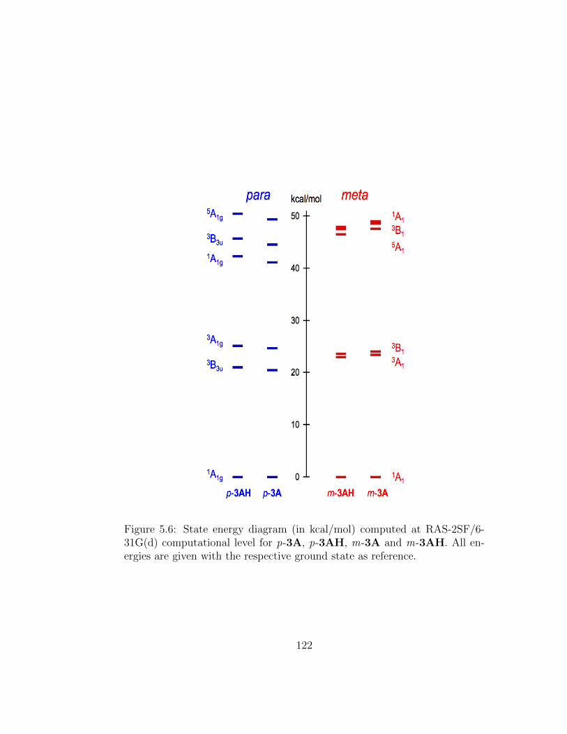
Figure 5.6: State energy diagram (in kcal/mol) computed at RAS-2SF/6-31G(d) computational level for p-3A, p-3AH, m-3A and m-3AH. All en-ergies are given with the respective ground state as reference.
122
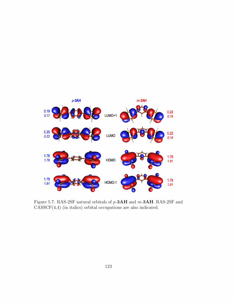
Figure 5.7: RAS-2SF natural orbitals of p-3AH and m-3AH. RAS-2SF andCASSCF(4,4) (in italics) orbital occupations are also indicated.
123
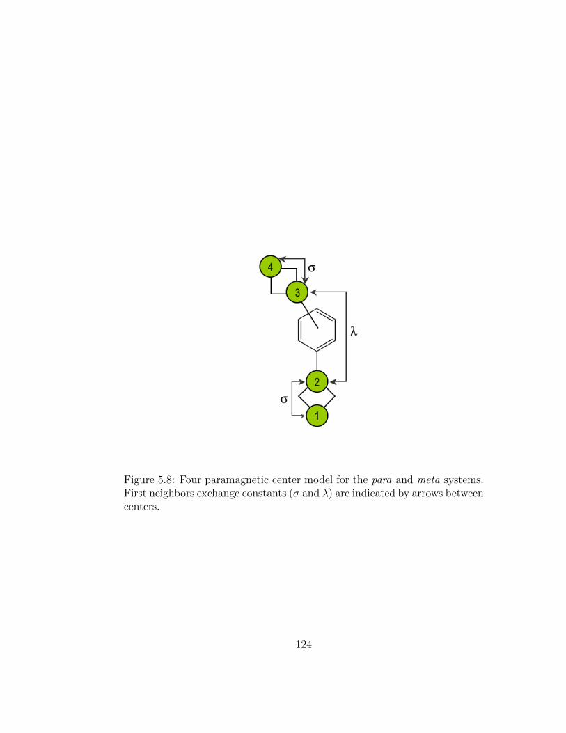
Figure 5.8: Four paramagnetic center model for the para and meta systems.First neighbors exchange constants (σ and λ) are indicated by arrows betweencenters.
124
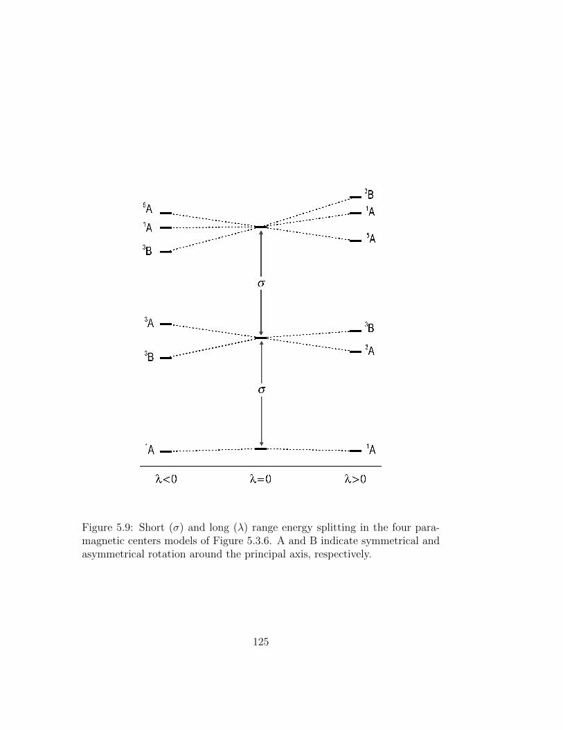
Figure 5.9: Short (σ) and long (λ) range energy splitting in the four para-magnetic centers models of Figure 5.3.6. A and B indicate symmetrical andasymmetrical rotation around the principal axis, respectively.
125

126
Chapter 6
Restricted Active SpaceSpin-Flip (RAS-SF) withArbitrary Number of Spin-Flips
6.1 Introduction
The most common electronic structure of molecules is when there is an appre-ciable gap between nominally filled and nominally empty molecular orbitals(MOs). In this case a single electron configuration of doubly occupied MOsis the correct zero order picture, and corrections, either by perturbation the-ory [15,16] or coupled cluster theory [23–27] account for the secondary effectsof electron correlation. However, electronic degeneracy or near-degeneracyof the nominally occupied and virtual orbitals is nonetheless widely encoun-tered in chemistry. Examples include bond dissociations, radicals and metalcomplexes.
(Near-)degeneracies lead to wavefunctions in which several determinantscontribute considerably, rather than just one configuration. Since most elec-tronic structure methods are based on a single reference, systems featuring(near-)degeneracies have been posing considerable challenges. Furthermore,another important consequence of near-degeneracy of occupied and virtualMOs is that there are very low-lying excited states. Treating both the groundstate and low-lying excited states in a balanced way is another challenge forelectronic structure theory. Problems in this category are often said to ex-
127
hibit strong electron correlations.
One of the simplest examples of electronic degeneracy is the dissociationof a σ bond, such as the hydrogen molecule, H2. At equilibrium, the (σ)2 con-figuration describes the wavefunction almost exclusively, whereas at the dis-sociation limit, the antibonding orbital, σ∗, is now degenerate and the (σ∗)2
configuration carries equal weight. Therefore, as the bond length increases, aminimum of two configurations need to be included to adequately describe thewavefunction. Alternatively, spin-unrestriction may be employed. This re-sults in improved energies over a single-determinant spin-restricted approach.However, often considerable spin-contamination and unreliable wave-functionproperties can be encountered, particularly for excited states [96].
In the past, multi-reference wavefunctions, such as the complete-active-space self-consistent-field (CASSCF) [50, 51] theory have been employed toovercome the challenges of single-determinant approaches. CASSCF, how-ever, suffers from several issues that hinders its application to complex,strongly correlated molecules. Firstly, the method scales exponentially withthe active space size. Therefore only calculations involving small activespaces (less than 17 orbitals) can be carried out to date. Secondly, the prob-lem of optimizing the active orbitals is often poorly convergent and com-putationally demanding. Other commonly encountered issues in CASSCFcalculations include the intruder state problem [66,67] and the need for state-averaging [56,57], when multiple states are sought.
Despite these limitations, CASSCF can be viewed as the appropriatesimplified Schrodinger equation to solve for the zero-order wavefunction instrongly correlated molecules. Therefore there is growing interest in tractableapproximations to CASSCF, of which we will discuss a few of the currentalternatives. Perhaps the simplest is the Restricted Active Space (RAS)[20,68–70] approach in which some excitations are discarded. Like most ap-proximate configuration interaction (CI) methods, it is not size-consistent,although useful results can be obtained when it is carefully applied. Coupled-cluster approximations to CASSCF are under active development, basedon a single reference (e.g. valence orbital optimized coupled-cluster (VOO-CC) [76–78], and their local variants, including perfect pairing (PP) [79,80],perfect quadruples (PQ) [80, 81], and perfect hextuples (PH) [80, 82]), aswell as true multi-reference coupled-cluster (MR-CC) methods [62–65]. The
128

density matrix renormalization group (DMRG) [31–38], as well as reduceddensity matrix methods [403–407] are other novel alternatives.
Recently, a family of methods based on the spin-flip (SF) approach [3,95,97–100, 408] has been introduced to address the issue of electronic degener-acy. In this theory, a restricted open-shell high-spin wavefunction is chosenas the reference. Contrary to the low-spin wavefunction, the high-spin wave-function can be chosen to be mainly single-reference in character at any nu-clear distance. Through spin-flipping, complex multi-configurational statesof lower spin multiplicity can be accessed. Therefore these methods are ableto address many multi-reference problems, while retaining the theoreticalsimplicity and computational speed of single reference approaches. Spin-flipversions of both CI [96,99,409,410] and CC [98,411,412] methods have beensuccessfully developed. At the single spin-flip level, these methods are widelyused. Here, biradicaloid singlet ground and excited states are accessed viaa high-spin triplet reference. Double spin-flip approaches, where a quintetreference is used to access strongly correlated singlet and triplet states, havealso been implemented [100].
While the above SF methods have wavefunctions that are strictly trun-cated by excitation level (e.g. SF-CIS, EOM-SF-CCSD, etc.), an alternativeversion based on the RAS concept, termed RAS-SF, has been recently intro-duced [3]. RAS-SF allows, in principle, excitations of any number of electronsin the half-occupied orbitals of the high-spin reference (the “RAS-II” space)as well as single excitations into RAS-II from lower doubly occupied MOs(“RAS-I”, which are also known as hole excitations) or single excitationsfrom RAS-II into higher empty MOs (“RAS-III”, also referred to as parti-cle excitations). In practice, however, the maximum number of spin flips inRAS-SF was restricted to two. At the level of 2 spin-flips (RAS-2SF), veryencouraging results were obtained for large tetraradicaloids [3].
Our work extends the number of possible spin flips and allows for a vari-able orbital active space. This has the exciting potential to provide accurate,spin-pure, wavefunction-based results in many areas that were inaccessibleso far, such as large polyradicals, three or more bond dissociation processes,as well as bi- or polynuclear-metal systems, which are of importance in bi-ology, catalysis [413] and materials science [414]. Due to their size, studiesof such complexes have been limited to calculations involving density func-
129

tional theory (DFT), which cannot properly describe strong electron corre-lation. Organic polyradicals have found great interest as potential magneticmaterials [415–419] or conductors [340, 345, 347–349], with the advantage oftunability by altering substituents and the potential of solubility in organicmedia.
In this paper several binuclear metal complexes, bond dissociation pro-cesses as well as organic polyradicals will be studied. The RAS-SF results arecompared to experimental values, other wavefunction-based, multi-referencemethods, such as DMRG, CASSCF, and CASPT2, as well as broken-symmetryDFT.
6.2 Theory
Our extension to the SF family is based on the formulation of the restrictedactive space spin-flip method by Casanova and Head-Gordon [3].
Writing the expansion for the general excitation operator R in termsof hole, particle, hole-particle, etc., excitations allows the SF method tobe formulated in the framework of a restricted active space configurationinteraction (RAS-CI) method.
RnSF =∑λ∈A
R∆MS=−nλ +
∑λ∈h
R∆MS=−nλ +∑
λ∈p
R∆MS=−nλ +
∑λ∈hp
R∆MS=−nλ + ...
(6.1)
In equation 6.1, A denotes all excitations in the active space, h excita-tion from a hole level to the active space, p particle excitations from theactive space to a particle level and hp hole-particle configurations. Activespaces with Ne electrons and No orbitals will be denoted as (Ne, No). Asshown schematically in Figure 6.1, equation 6.1 divides the orbital space intothree subspaces labelled I through III (if the frozen core technique is applied,four subspaces result). The minimum and maximum occupancies in each sub-space is determined by the maximum number of hole and particle excitations.
In order to have linear scaling outside the active space (RAS-I and III)
130
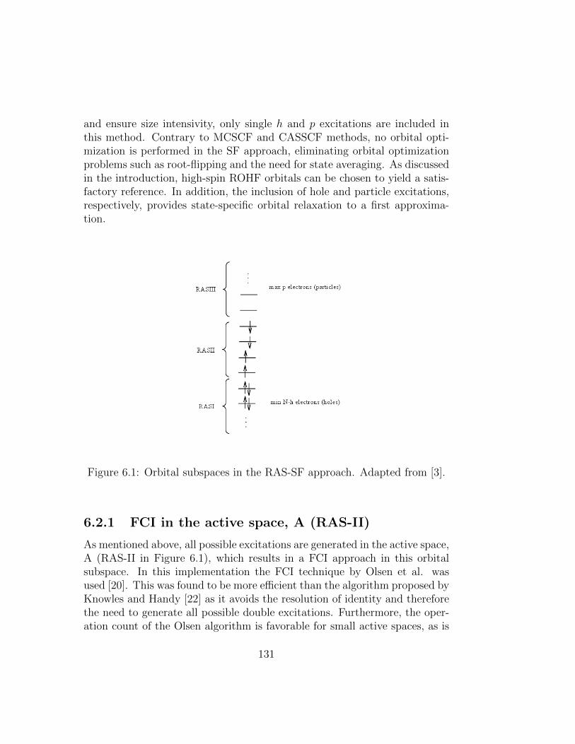
and ensure size intensivity, only single h and p excitations are included inthis method. Contrary to MCSCF and CASSCF methods, no orbital opti-mization is performed in the SF approach, eliminating orbital optimizationproblems such as root-flipping and the need for state averaging. As discussedin the introduction, high-spin ROHF orbitals can be chosen to yield a satis-factory reference. In addition, the inclusion of hole and particle excitations,respectively, provides state-specific orbital relaxation to a first approxima-tion.
Figure 6.1: Orbital subspaces in the RAS-SF approach. Adapted from [3].
6.2.1 FCI in the active space, A (RAS-II)
As mentioned above, all possible excitations are generated in the active space,A (RAS-II in Figure 6.1), which results in a FCI approach in this orbitalsubspace. In this implementation the FCI technique by Olsen et al. wasused [20]. This was found to be more efficient than the algorithm proposed byKnowles and Handy [22] as it avoids the resolution of identity and thereforethe need to generate all possible double excitations. Furthermore, the oper-ation count of the Olsen algorithm is favorable for small active spaces, as is
131

the case here. Both of these factors outweigh the computational speed-up re-sulting from matrix-matrix multiplications in the Handy-Knowles algorithmcompared to the vector-matrix approach used by Olsen and co-workers. Theα and β strings are generated using the algorithm proposed by Ruedenberget al. [420], which was slightly modified to account for hole and particle con-tributions from the RAS-I and III spaces. The guess vector for the Davidsonalgorithm is generated by diagonalizing the RAS-II space, and if memorypermits hole and particle excitations are also included. Algorithmic detailsand computational timings for the general implementation of the RAS-SFmethod presented here will be given elsewhere [421].
6.2.2 Properties of RAS-SF
As discussed in previous work [3], RAS-SF features many of the desirableproperties an electronic structure theory ought to have. It is multistate,spin-complete, variational, size consistent, and orbital invariant within theRAS subspaces. The size-consistency/intensivity property for a fixed num-ber of spin-flips is particularly special and reflects the fact that RAS-SFis constructed analogously to CIS, another rare example of a truncated CImodel that is size-consistent. It is also worth mentioning that the RAS-SFmethod mainly captures static correlation and lacks dynamical correlation.Extensions to recover dynamical correlation would be highly desirable.
6.3 Computational Details
All calculations have been carried out using a developer’s version of Q-Chem3.0 [311]. For computational speed-up resolution-of-the-identity (RI) inte-grals [158, 159] have been used. All RAS-SF calculations were carried outusing a restricted open shell (ROHF) high-spin reference. Unless indicated,all electrons were included (no frozen core or frozen virtual spaces were em-ployed). For metal complexes, single point calculations on the X-ray crystalgeometries have been carried out to determine the exchange coupling con-stants, as is typical for such calculations.
132

6.4 Results and Discussion
6.4.1 Bond Dissociation
The ability to perform beyond two spin flips allows bond dissociation pro-cesses of three or more bonds to be described. Figure 6.2 shows the dis-sociation curve for the N2 molecule. Comparison with CASSCF(6,6) calcu-lations [422] show extremely good agreement with RAS-SF(6,6) results. Inorder to understand the effect of orbitals on RAS-SF, numerical results basedon restricted singlet and septet references are shown, respectively. Interest-ingly, both guesses yield similar results. However, only the ROHF orbitalsdissociate to the correct limit of two nitrogen atoms.
Figure 6.2: Dissociation curve for the N2 molecule (cc-pVTZ)
133

6.4.2 Binuclear Metal Complexes
When properties of transition metal complexes are studied, the exchange cou-pling between different sites is a sought after quantity. To extract this quan-tity, typically, data obtained from neutron diffraction, Raman spectroscopy,magnetic susceptibility and electron paramagnetic resonance measurementsis fitted to the model Heisenberg-Dirac-Van Vleck spin-only Hamilitonian,which takes the form [423–425]
H = −2∑i>j
JijSiSj (6.2)
where Si and Sj are the spin operators on sites i and j, respectively. Jij isthe exchange coupling, which may be negative, indicating antiferromagneticcoupling or positive, which is related to ferromagnetic coupling [426]. Caremust be taken when comparing to coupling constants cited in the literature,as the factor of 2 in the model Hamiltonian given in equation 6.2 is some-times incorporated in the coupling constants.
From a theoretical point of view, most wavefunction methods that wouldbe suitable for these types of problems are computationally too expensivegiven the size of typical bi- or polynuclear metal complexes. Therefore,density-functional theory (DFT) is typically used to compute the exchangecouplings. In this approach, broken symmetry solutions enter the equationsto account for states that exhibit multideterminantal character. These, how-ever, are artifacts of the approximate nature of the exchange-correlationfunctionals and several different expressions are used to extract the mag-netic coupling parameters [427–431].
An alternative approach, based on constrained DFT has recently beenshown to be successful in predicting exchange coupling constants in a num-ber of binuclear metal complexes [432].
In the remainder of this section the coupling constants for several biuclearmetal complexes will be computed using the RAS-SF method and comparedto experimental, DFT and CASSCF results.
134
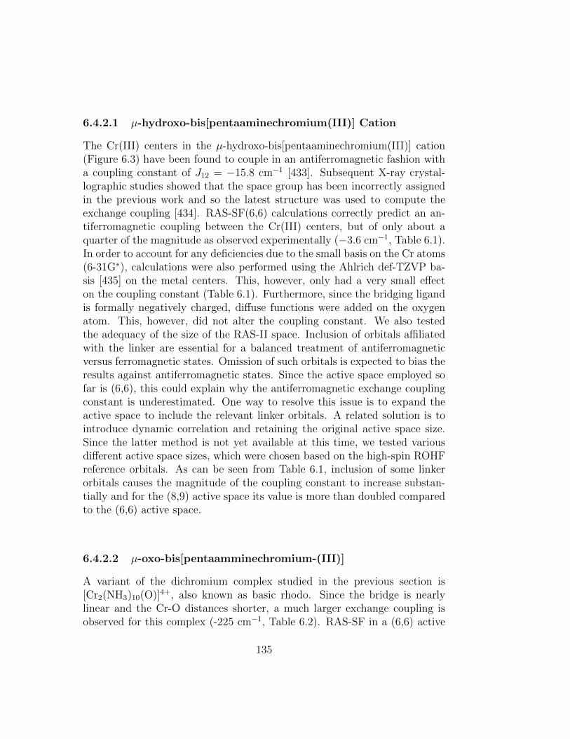
6.4.2.1 µ-hydroxo-bis[pentaaminechromium(III)] Cation
The Cr(III) centers in the µ-hydroxo-bis[pentaaminechromium(III)] cation(Figure 6.3) have been found to couple in an antiferromagnetic fashion witha coupling constant of J12 = −15.8 cm−1 [433]. Subsequent X-ray crystal-lographic studies showed that the space group has been incorrectly assignedin the previous work and so the latest structure was used to compute theexchange coupling [434]. RAS-SF(6,6) calculations correctly predict an an-tiferromagnetic coupling between the Cr(III) centers, but of only about aquarter of the magnitude as observed experimentally (−3.6 cm−1, Table 6.1).In order to account for any deficiencies due to the small basis on the Cr atoms(6-31G∗), calculations were also performed using the Ahlrich def-TZVP ba-sis [435] on the metal centers. This, however, only had a very small effecton the coupling constant (Table 6.1). Furthermore, since the bridging ligandis formally negatively charged, diffuse functions were added on the oxygenatom. This, however, did not alter the coupling constant. We also testedthe adequacy of the size of the RAS-II space. Inclusion of orbitals affiliatedwith the linker are essential for a balanced treatment of antiferromagneticversus ferromagnetic states. Omission of such orbitals is expected to bias theresults against antiferromagnetic states. Since the active space employed sofar is (6,6), this could explain why the antiferromagnetic exchange couplingconstant is underestimated. One way to resolve this issue is to expand theactive space to include the relevant linker orbitals. A related solution is tointroduce dynamic correlation and retaining the original active space size.Since the latter method is not yet available at this time, we tested variousdifferent active space sizes, which were chosen based on the high-spin ROHFreference orbitals. As can be seen from Table 6.1, inclusion of some linkerorbitals causes the magnitude of the coupling constant to increase substan-tially and for the (8,9) active space its value is more than doubled comparedto the (6,6) active space.
6.4.2.2 µ-oxo-bis[pentaamminechromium-(III)]
A variant of the dichromium complex studied in the previous section is[Cr2(NH3)10(O)]4+, also known as basic rhodo. Since the bridge is nearlylinear and the Cr-O distances shorter, a much larger exchange coupling isobserved for this complex (-225 cm−1, Table 6.2). RAS-SF in a (6,6) active
135
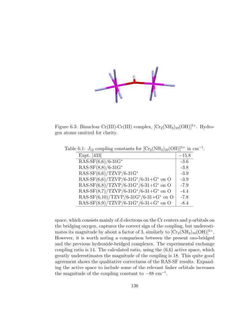
Figure 6.3: Binuclear Cr(III)-Cr(III) complex, [Cr2(NH3)10(OH)]5+. Hydro-gen atoms omitted for clarity.
Table 6.1: J12 coupling constants for [Cr2(NH3)10(OH)]5+ in cm−1.
Expt. [433] −15.8RAS-SF(6,6)/6-31G∗ -3.6RAS-SF(8,8)/6-31G∗ -3.8RAS-SF(6,6)/TZVP/6-31G∗ -3.9RAS-SF(6,6)/TZVP/6-31G∗/6-31+G∗ on O -3.9RAS-SF(6,8)/TZVP/6-31G∗/6-31+G∗ on O -7.9RAS-SF(8,7)/TZVP/6-31G∗/6-31+G∗ on O -4.4RAS-SF(6,10)/TZVP/6-31G∗/6-31+G∗ on O -7.8RAS-SF(8,9)/TZVP/6-31G∗/6-31+G∗ on O -8.4
space, which consists mainly of d electrons on the Cr centers and p orbitals onthe bridging oxygen, captures the correct sign of the coupling, but underesti-mates its magnitude by about a factor of 3, similarly to [Cr2(NH3)10(OH)]5+.However, it is worth noting a comparison between the present oxo-bridgedand the previous hydroxide-bridged complexes. The experimental exchangecoupling ratio is 14. The calculated ratio, using the (6,6) active space, whichgreatly underestimates the magnitude of the coupling is 18. This quite goodagreement shows the qualitative correctness of the RAS-SF results. Expand-ing the active space to include some of the relevant linker orbitals increasesthe magnitude of the coupling constant to −88 cm−1.
136
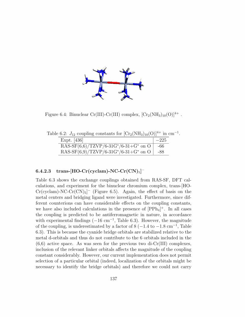
Figure 6.4: Binuclear Cr(III)-Cr(III) complex, [Cr2(NH3)10(O)]4+ .
Table 6.2: J12 coupling constants for [Cr2(NH3)10(O)]4+ in cm−1.
Expt. [436] −225RAS-SF(6,6)/TZVP/6-31G∗/6-31+G∗ on O -66RAS-SF(6,9)/TZVP/6-31G∗/6-31+G∗ on O -88
6.4.2.3 trans-[HO-Cr(cyclam)-NC-Cr(CN)5]−
Table 6.3 shows the exchange couplings obtained from RAS-SF, DFT cal-culations, and experiment for the binuclear chromium complex, trans-[HO-Cr(cyclam)-NC-Cr(CN)5]− (Figure 6.5). Again, the effect of basis on themetal centers and bridging ligand were investigated. Furthermore, since dif-ferent counterions can have considerable effects on the coupling constants,we have also included calculations in the presence of [PPh4]+. In all casesthe coupling is predicted to be antiferromagnetic in nature, in accordancewith experimental findings (−16 cm−1, Table 6.3). However, the magnitudeof the coupling, is underestimated by a factor of 8 (−1.4 to −1.8 cm−1, Table6.3). This is because the cyanide bridge orbitals are stabilized relative to themetal d-orbitals and thus do not contribute to the 6 orbitals included in the(6,6) active space. As was seen for the previous two di-Cr(III) complexes,inclusion of the relevant linker orbitals affects the magnitude of the couplingconstant considerably. However, our current implementation does not permitselection of a particular orbital (indeed, localization of the orbitals might benecessary to identify the bridge orbitals) and therefore we could not carry
137
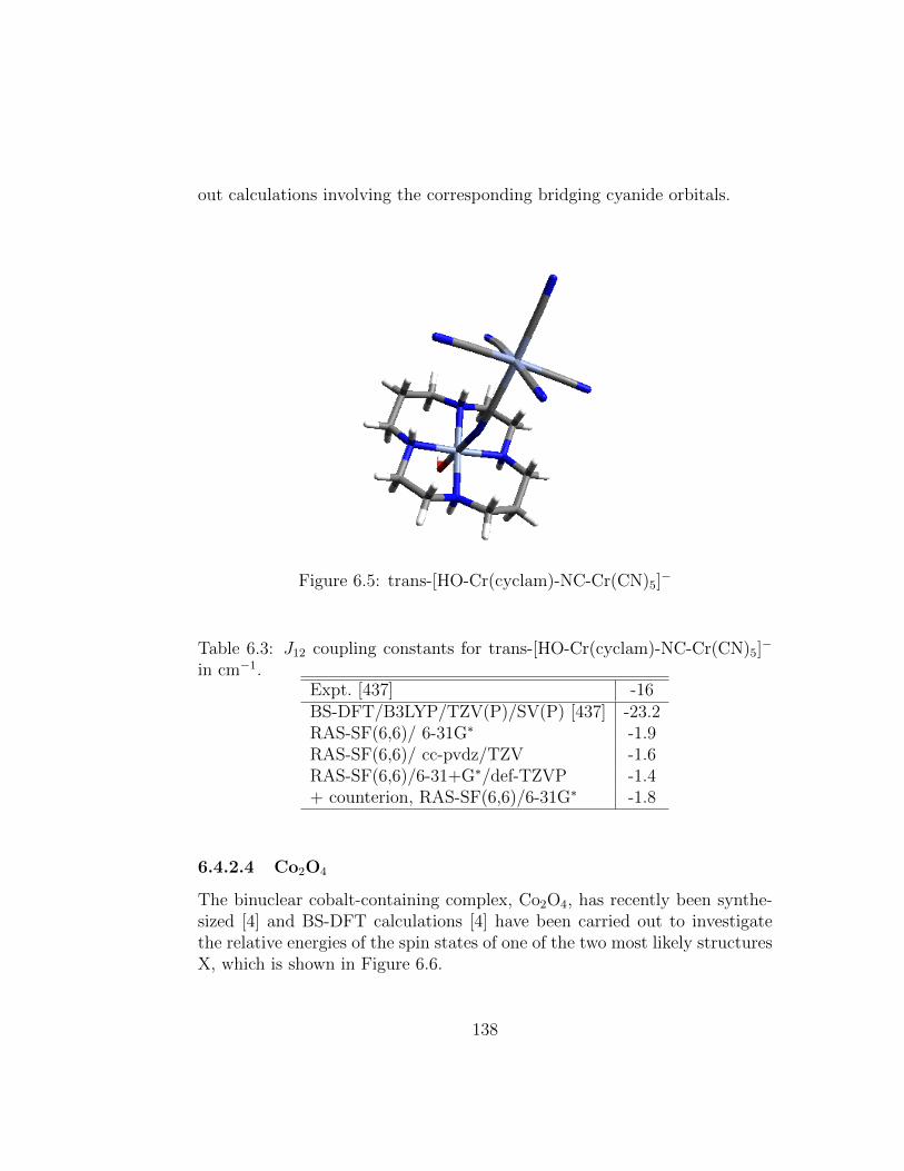
out calculations involving the corresponding bridging cyanide orbitals.
Figure 6.5: trans-[HO-Cr(cyclam)-NC-Cr(CN)5]−
Table 6.3: J12 coupling constants for trans-[HO-Cr(cyclam)-NC-Cr(CN)5]−
in cm−1.Expt. [437] -16BS-DFT/B3LYP/TZV(P)/SV(P) [437] -23.2RAS-SF(6,6)/ 6-31G∗ -1.9RAS-SF(6,6)/ cc-pvdz/TZV -1.6RAS-SF(6,6)/6-31+G∗/def-TZVP -1.4+ counterion, RAS-SF(6,6)/6-31G∗ -1.8
6.4.2.4 Co2O4
The binuclear cobalt-containing complex, Co2O4, has recently been synthe-sized [4] and BS-DFT calculations [4] have been carried out to investigatethe relative energies of the spin states of one of the two most likely structuresX, which is shown in Figure 6.6.
138

Figure 6.6: Co2O4. Structure from [4].
BS-DFT and RAS-SF calculations predict a similar ordering of the spinstates (Table 6.4). Only the quintet and triplet states are swapped betweenthe two methods. Also, the singlet-nonet energy gap is similar for both BS-DFT and RAS-SF methods (between 27.7 and 29.2 kcal/mol). However,RAS-SF predicts the other spin states to be almost degenerate with thesinglet ground state, which stands in contrast to the results obtained fromBS-DFT (Table 6.4). Based on the previous study of the binuclear Cr(III)complexes, we expect the coupling obtained from RAS-SF to be underesti-mated, as we have not included all relevant orbitals from the bridging oxides.
Table 6.4: Ground and excited states for structure X of Co2O4 (in inkcal/mol) (Figure 6.6). BS-DFT results from [4].
6-31G∗ 6-31G∗ TZVP/cc-pVDZState (〈S2〉) BS-DFT RAS-SF(6,6) RAS-SF(8,8) RAS-SF(8,8)
0 0.0 0.00 0.00 0.006 3.3 0.15 0.56 0.622 4.9 0.05 0.18 0.2012 9.3 0.29 1.16 1.2920 27.7 - 29.2 27.8
6.4.2.5 [(TPA*)Co(II)(DHBQ2−)Co(II)(TPA*)]2+
The binuclear-cobalt(II) complex [(TPA*)Co(II)(DHBQ2−)Co(II)(TPA*)]2+
(Figure 6.7) was also investigated, where TPA* = tris[(3,5-dimethyl-pyrazol-1-yl)methyl)] amine, and DHBQ = deprotonated 2,5-dihydroxy-1,4-benzoquinone.
139

The experimental exchange coupling constant for this cobalt complex is foundto be very small in magnitude and antiferromagnetic in nature (−1.91 cm−1,Table 6.5). RAS-SF(6,6) calculations also predict an antiferromagnetic cou-pling between the two Co(II) centers, but as for the other metal complexesdiscussed previously, the magnitude of the coupling is underestimated foraforementioned reasons.
Figure 6.7: Binuclear Co2(II) complex,[(TPA*)Co(II)(DHBQ2−)CO(II)(TPA*)]2+
Table 6.5: J12 coupling constants for[(TPA*)Co(II)(DHBQ2−)Co(II)(TPA*)]2+ in cm−1.
Expt. [438] −1.91RAS-SF(6,6)/6-31G∗ -0.3
6.4.3 Organic Polyradicals
High-spin organic polyradicals have gained considerable interest as they maylead to novel magnetic materials [415–419]. Both intra- as well as inter-molecular spin coupling have been pursued, with the former posing a morepromising route [417,418,439]. In attempts to forming extensive intramolecu-lar high-spin systems, one-dimensional poly(m-phenylenecarbenes) and two-dimensional branched carbenes (Figure 6.8) have been synthesized, which are
140
all found experimentally to exhibit high-spin ground states [440–443]. Typi-cally the m-phenylene moiety is used as a linker as it is one of the strongestferromagnetic coupling units. The exchange coupling, Jij, between the thespin sites, as introduced in equation 6.2 is one of the important propertiesto be determined in such systems, as it will gauge their applicability as mag-netic materials.
6.4.3.1 Linear Carbenes
We studied the ground- and excited-states of linear poly(m-phenylenecarbenes)n = 1−5, Figure 6.8. Cholesky decomposition based CASSCF (CD-CASSCF)and DMRG calculations have been previously carried out for geometries con-strained to the C2v point group (Table 6.6). Very good agreement betweenour RAS-SF results and those obtained from CD-CASSCF is obtained (thesame active space size was used for both methods). In all cases studied, thehigh-spin ground state is predicted to be the lowest in energy, in accordancewith experimental findings. As can be seen in Table 6.6, CD-CASPT2 yieldsvery similar results to CD-CASSCF, suggesting that dynamic correlation isnot very important in these systems. Therefore, we expect that increasingthe active space size of our RAS-SF calculations to include the π orbitalsfrom the benzene linkers will not affect the energy gaps considerably. How-ever, unlike DMRG, CD-CASPT2 and CD-CASSCF, the RAS-SF results donot show an odd-even oscillation in the spin energy gaps (Table 6.6).
However, the actual geometry for these carbenes deviates strongly fromC2v symmetry, which was applied for computational savings. Deviation fromplanarity is expected to affect the delocalization and thus the exchange cou-pling, i.e. the relative energies of the various spin states. We thereforealso carried out RAS-SF calculation on re-optimized structures (UB3LYP/6-31G∗) of linear carbenes n = 1 − 5 (Figure 6.8), which will be referred toas C1 structures. Since the RAS-SF, CASSCF and DMRG results for theC2v structures agreed very well, we expect the RAS-SF results for the C1structures to yield very similar results also, yet obtained with greater com-putational ease. Relative RAS-SF energies and selected UB3LYP geometricparameters are shown in Tables 6.7 to 6.10. The dihedral angles given arethose spanned by two adjacent benzene moieties and the carbene unit andthe angles refer to the angles in the carbene unit.
141

The largest energy change associated with the variation of a geometricparameter is observed for the singlet-triplet gap in carbene n = 1. Here,opening the angle from 119◦ to 142◦ in the C1 structures (Table 6.7) causesthe singlet-triplet energy gap to increase from 3.76 kcal/mol to 25.8 kcal/mol.Whereas similar changes in angle is also observed for the larger carbenes (e.g.n = 3, (Table 6.9)), the relative energy differences between the various spin-states remain very similar in these cases (e.g. Table 6.9).
The geometric parameters between the C2v and C1 structures of the samespin multiplicity are considerably different (Tables 6.7 to 6.10). The dihedralangles, which are restricted to 0◦ in the C2v structures, relax to 27− 37◦ inthe C1 geometries. This allows the angles around the carbene moiety to besmaller in the case of the C1 structures. Despite these geometric differences,the relative energies between the spin states differ by at most 4 kcal/mol.However, for longer carbenes, where the energy gaps are very small, this cancause the energy difference to be overestimated by a factor of 2.5. In general,the C2v geometries overestimate the coupling between the units as the pla-narity maximizes the interaction between the π system of the carbene unitsand the benzene rings.
Finally, for n = 3 and n = 4 we also compared our RAS-SF results to twodensity functionals (UB3LYP and UBP86). Values for n = 3 are given inTables 6.11 and 6.12, and for n = 4 in Table 6.10. The energy gaps predictedby UB3LYP and UBP86 are considerably larger than those obtained fromRAS-SF studies. The relative energies computed by DFT are also foundto be much more sensitive towards geometrical changes. In some cases thiscauses even the ordering of the spin states to switch. Noteworthy is also,that BP86 features considerable spin contamination, especially for the lowerspin multiplicities. Furthermore, the two density functionals, when com-pared to each other, yield substantially different results. For example, thesinglet-septet energy gaps for the S=3 geometry are 35.4 and 9.63 kcal/molfor UB3LYP and UBP86, respectively (Tables 6.11 and 6.12), and for n = 4,UBP86 predicts a completely different ordering of the spin states comparedto RAS-SF and UB3LYP (Table 6.10). This highlights the need for a methodthat can reliably predict spin state energies and is systematically improvable.
142

Figure 6.8: One- and two-dimensional carbenes. (n = 1− 5, m = 3, 6, 9)
Table 6.6: Relative energies (kcal/mol) between S=n and S=0 states of linearn-carbenes n = 1 − 4 (Figure 6.8). Geometries restricted to the C2v pointgroup.
n 1 2 3 4CD-CASSCF [444] -26.0 -2.72 -4.19 -2.47CD-CASPT2 [444] -18.8 -3.31 -5.58 -1.24DMRG-SCF [444] -21.5 -6.95 -8.63 -5.02
RAS-SF -25.8 -3.56 -3.47 -1.95
6.4.3.2 Branched Carbenes
6.4.3.2.1 Polycarbene m = 3
Branched systems such as the two-dimensional carbenes and Closs-radicals,which will be discussed in the next section, are of particularly great interestto us, as the broken-symmetry DFT approaches are not applicable to suchsystems. Table 6.13 lists the relative energies obtained from RAS-SF(6,6)calculations for the two-dimensional polycarbene with m = 3, Figure 6.8.The relative energies are found to be quite insensitive towards geometricalchanges. In accordance with experimental findings, the ground state is pre-dicted to be a septet. The other spin states lie in close proximity, indicatingweak coupling between the spin centers. Comparison to UB3LYP calcula-tions shows that RAS-SF again tends to predict considerably smaller energygaps, although the ordering of the spin states is predicted to be the same for
143
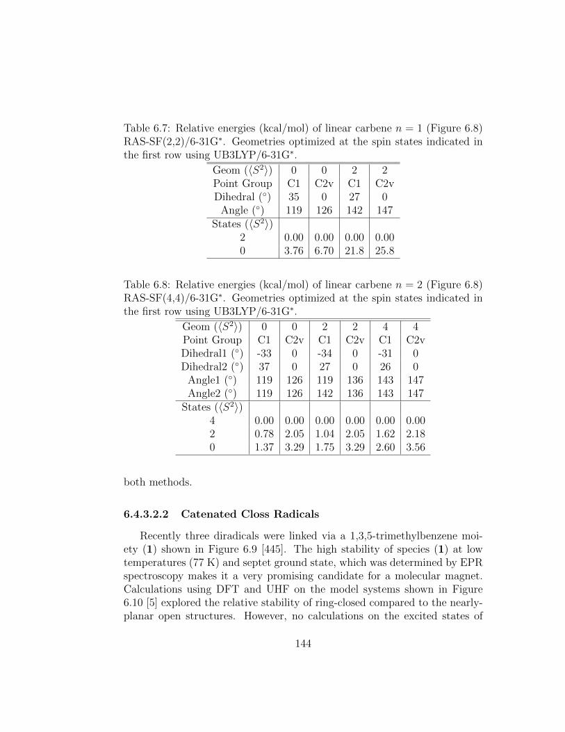
Table 6.7: Relative energies (kcal/mol) of linear carbene n = 1 (Figure 6.8)RAS-SF(2,2)/6-31G∗. Geometries optimized at the spin states indicated inthe first row using UB3LYP/6-31G∗.
Geom (〈S2〉) 0 0 2 2Point Group C1 C2v C1 C2vDihedral (◦) 35 0 27 0
Angle (◦) 119 126 142 147States (〈S2〉)
2 0.00 0.00 0.00 0.000 3.76 6.70 21.8 25.8
Table 6.8: Relative energies (kcal/mol) of linear carbene n = 2 (Figure 6.8)RAS-SF(4,4)/6-31G∗. Geometries optimized at the spin states indicated inthe first row using UB3LYP/6-31G∗.
Geom (〈S2〉) 0 0 2 2 4 4Point Group C1 C2v C1 C2v C1 C2vDihedral1 (◦) -33 0 -34 0 -31 0Dihedral2 (◦) 37 0 27 0 26 0
Angle1 (◦) 119 126 119 136 143 147Angle2 (◦) 119 126 142 136 143 147
States (〈S2〉)4 0.00 0.00 0.00 0.00 0.00 0.002 0.78 2.05 1.04 2.05 1.62 2.180 1.37 3.29 1.75 3.29 2.60 3.56
both methods.
6.4.3.2.2 Catenated Closs Radicals
Recently three diradicals were linked via a 1,3,5-trimethylbenzene moi-ety (1) shown in Figure 6.9 [445]. The high stability of species (1) at lowtemperatures (77 K) and septet ground state, which was determined by EPRspectroscopy makes it a very promising candidate for a molecular magnet.Calculations using DFT and UHF on the model systems shown in Figure6.10 [5] explored the relative stability of ring-closed compared to the nearly-planar open structures. However, no calculations on the excited states of
144

Table 6.9: Relative energies (kcal/mol) of linear carbene n = 3 (Figure 6.8)RAS-SF(6,6)/6-31G∗. Geometries optimized at the spin states indicated inthe first row using UB3LYP/6-31G∗.
Geometry (〈S2〉) 0 2 6 12 12Point Group C1 C1 C1 C1 C2vDihedral1 (◦) -33 -34 -34 -31 0Dihedral2 (◦) 35 29 30 29 0Dihedral3 (◦) -37 -38 -26 -26 0
Angle1 (◦) 119 129 143 143 147Angle2 (◦) 119 143 143 143 147Angle3 (◦) 119 129 143 143 147
States (〈S2〉)12 0.00 0.00 0.00 0.00 0.006 0.40 0.60 0.70 0.79 0.852 0.81 1.23 1.41 1.61 1.726 1.27 1.84 2.18 2.41 2.392 1.33 1.92 2.30 2.50 2.560 1.42 2.42 2.86 3.17 3.472 2.09 3.17 3.78 4.17 4.43
species (1) have been performed.
Since the septet is experimentally found to be prevalent, we investigatedthe energy differences between the various spin states for the S=3 geometry,which are related to the spin-coupling within each molecule. Since the phenylgroups are expected to affect the stability of the high-spin states considerablyas they allow delocalization over the π system, calculations were carried outon the full system (Figure 6.9). As in the previous part, RAS(6,6), UB3LYP,UBP86 and UHF calculations were studied. As can be seen from Table 6.14,all methods predict the septet state to be the ground state, in accordancewith experimental findings. However, as was already observed in other ex-amples, RAS-SF predicts substantially smaller energy differences betweenthe various spin states compared to the density functionals under consider-ation. The singlet-septet gap, for example, is 0.86, 72.2, and 6.13 kcal/molfor RAS-SF(6,6), UB3LYP, and UBP86, respectively (Table 6.14). However,the two functionals again vary considerably in their predictions and feature
145

Table 6.10: Relative energies (kcal/mol) of linear carbene n = 4 (Figure 6.8)RAS-SF(8,8)/6-31G∗. Geometries optimized at 〈S2〉 = 20 using UB3LYP/6-31G∗. 〈S2〉 given in parentheses for unrestricted calculations.
RAS-SF UB3LYP UBP86Point Group C1 C2v C1 C1Dihedral1 (◦) -24 0 -24 -24Dihedral2 (◦) 20 0 20 20Dihedral3 (◦) -23 0 -23 -23Dihedral4 (◦) -20 0 -20 -20
Angle (◦) 138 141 138 138States (〈S2〉)
20 0.00 0.00 0.00 (20.2) 0.00 (20.1)12 0.48 0.73 18.6 (12.2) 5.98 (13.0)6 0.99 1.00 13.8 (7.8)2 1.12 1.54 44.5 (3.8) 6.61 (5.0)12 1.21 1.61 - -0 1.42 1.95 30.5 (3.5) 2.82 (4.1)6 1.46 1.98 - -
considerable spin contamination. We believe that the minimal (6,6) activespace used in the RAS-SF calculations may result in an underestimation ofthe relative energies of the spin states. Inclusion of the 3 π orbitals fromthe central benzene moiety into the RAS-II space is expected to result instronger coupling between the three biradical units.
6.5 Conclusions
Benchmark calculations on a triple bond dissociation, various binuclear metalsystems, and organic polyradicals were carried out using a new implementa-tion of the restricted active space spin-flip (RAS-SF) method, which allowsfor variable orbital active spaces and the study of systems requiring three ormore spin-flips.
Comparison of RAS-SF to other wave-function based, multi-referencemethods, such as CASSCF and DMRG yielded very good agreement, pro-
146
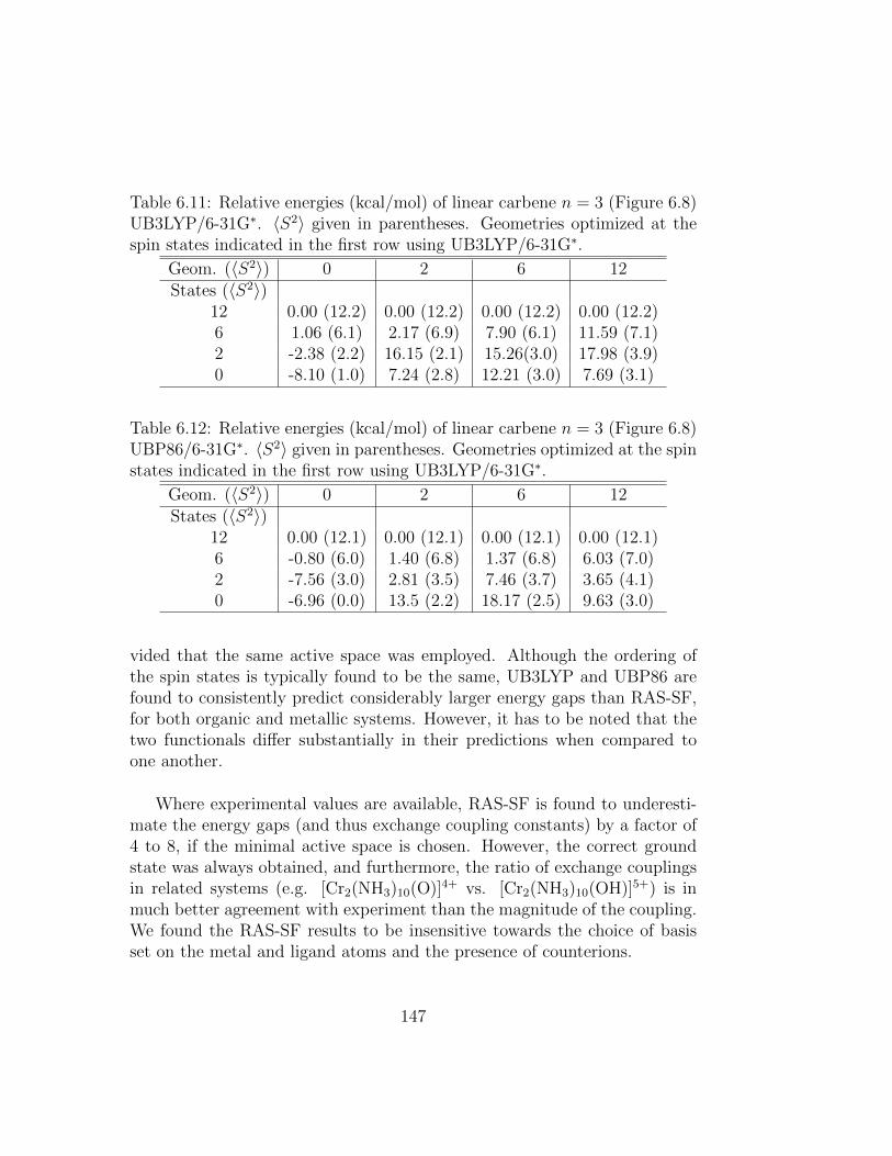
Table 6.11: Relative energies (kcal/mol) of linear carbene n = 3 (Figure 6.8)UB3LYP/6-31G∗. 〈S2〉 given in parentheses. Geometries optimized at thespin states indicated in the first row using UB3LYP/6-31G∗.
Geom. (〈S2〉) 0 2 6 12States (〈S2〉)
12 0.00 (12.2) 0.00 (12.2) 0.00 (12.2) 0.00 (12.2)6 1.06 (6.1) 2.17 (6.9) 7.90 (6.1) 11.59 (7.1)2 -2.38 (2.2) 16.15 (2.1) 15.26(3.0) 17.98 (3.9)0 -8.10 (1.0) 7.24 (2.8) 12.21 (3.0) 7.69 (3.1)
Table 6.12: Relative energies (kcal/mol) of linear carbene n = 3 (Figure 6.8)UBP86/6-31G∗. 〈S2〉 given in parentheses. Geometries optimized at the spinstates indicated in the first row using UB3LYP/6-31G∗.
Geom. (〈S2〉) 0 2 6 12States (〈S2〉)
12 0.00 (12.1) 0.00 (12.1) 0.00 (12.1) 0.00 (12.1)6 -0.80 (6.0) 1.40 (6.8) 1.37 (6.8) 6.03 (7.0)2 -7.56 (3.0) 2.81 (3.5) 7.46 (3.7) 3.65 (4.1)0 -6.96 (0.0) 13.5 (2.2) 18.17 (2.5) 9.63 (3.0)
vided that the same active space was employed. Although the ordering ofthe spin states is typically found to be the same, UB3LYP and UBP86 arefound to consistently predict considerably larger energy gaps than RAS-SF,for both organic and metallic systems. However, it has to be noted that thetwo functionals differ substantially in their predictions when compared toone another.
Where experimental values are available, RAS-SF is found to underesti-mate the energy gaps (and thus exchange coupling constants) by a factor of4 to 8, if the minimal active space is chosen. However, the correct groundstate was always obtained, and furthermore, the ratio of exchange couplingsin related systems (e.g. [Cr2(NH3)10(O)]4+ vs. [Cr2(NH3)10(OH)]5+) is inmuch better agreement with experiment than the magnitude of the coupling.We found the RAS-SF results to be insensitive towards the choice of basisset on the metal and ligand atoms and the presence of counterions.
147
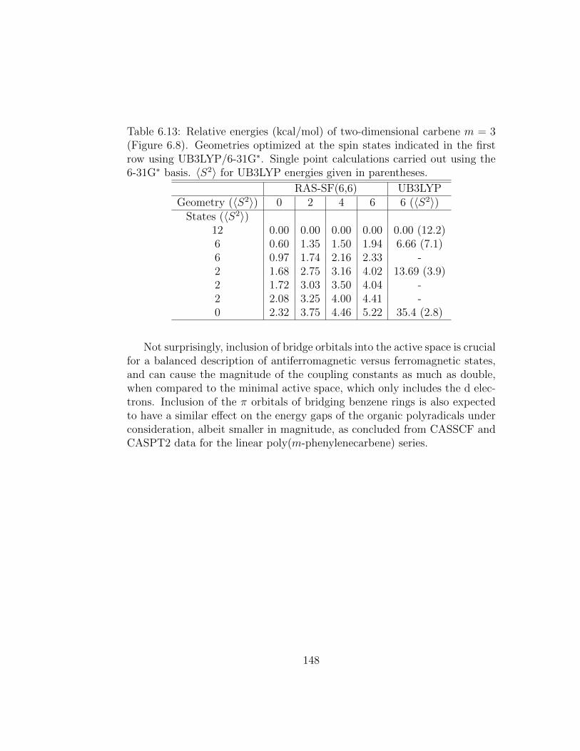
Table 6.13: Relative energies (kcal/mol) of two-dimensional carbene m = 3(Figure 6.8). Geometries optimized at the spin states indicated in the firstrow using UB3LYP/6-31G∗. Single point calculations carried out using the6-31G∗ basis. 〈S2〉 for UB3LYP energies given in parentheses.
RAS-SF(6,6) UB3LYPGeometry (〈S2〉) 0 2 4 6 6 (〈S2〉)
States (〈S2〉)12 0.00 0.00 0.00 0.00 0.00 (12.2)6 0.60 1.35 1.50 1.94 6.66 (7.1)6 0.97 1.74 2.16 2.33 -2 1.68 2.75 3.16 4.02 13.69 (3.9)2 1.72 3.03 3.50 4.04 -2 2.08 3.25 4.00 4.41 -0 2.32 3.75 4.46 5.22 35.4 (2.8)
Not surprisingly, inclusion of bridge orbitals into the active space is crucialfor a balanced description of antiferromagnetic versus ferromagnetic states,and can cause the magnitude of the coupling constants as much as double,when compared to the minimal active space, which only includes the d elec-trons. Inclusion of the π orbitals of bridging benzene rings is also expectedto have a similar effect on the energy gaps of the organic polyradicals underconsideration, albeit smaller in magnitude, as concluded from CASSCF andCASPT2 data for the linear poly(m-phenylenecarbene) series.
148
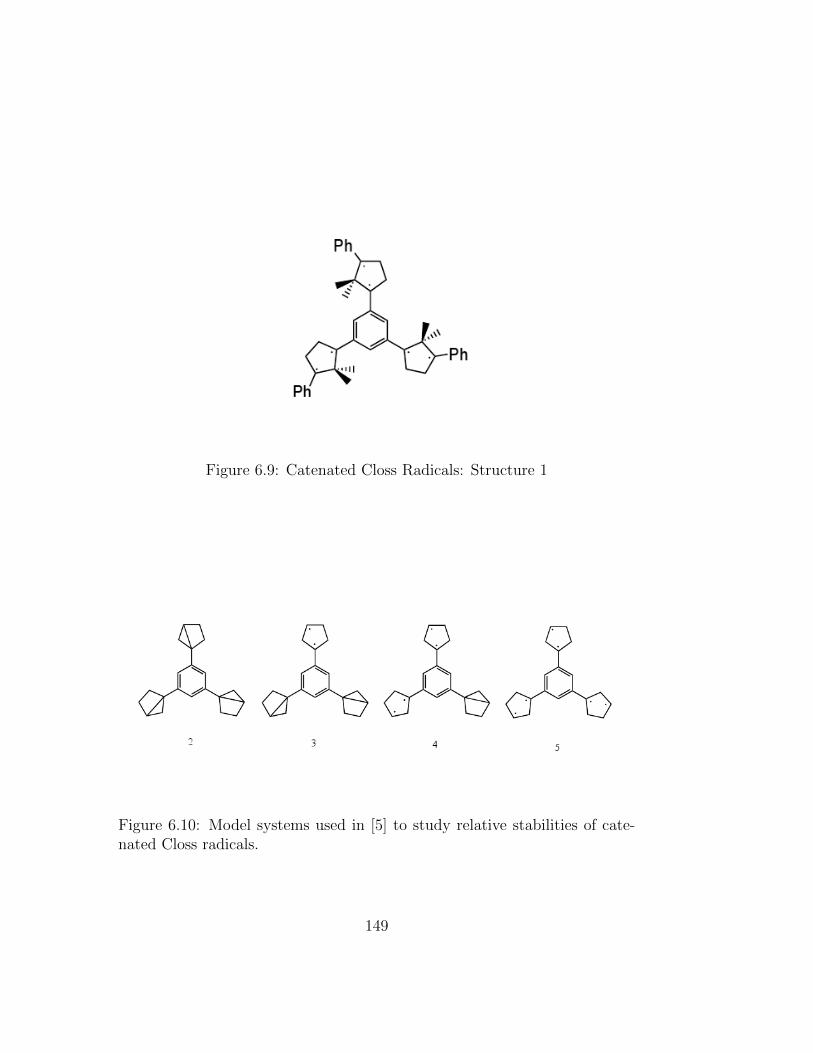
Figure 6.9: Catenated Closs Radicals: Structure 1
Figure 6.10: Model systems used in [5] to study relative stabilities of cate-nated Closs radicals.
149
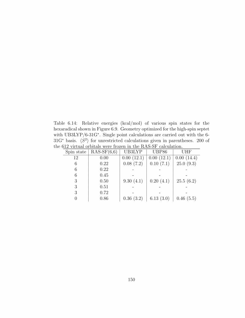
Table 6.14: Relative energies (kcal/mol) of various spin states for thehexaradical shown in Figure 6.9. Geometry optimized for the high-spin septetwith UB3LYP/6-31G∗. Single point calculations are carried out with the 6-31G∗ basis. 〈S2〉 for unrestricted calculations given in parentheses. 200 ofthe 612 virtual orbitals were frozen in the RAS-SF calculation.
Spin state RAS-SF(6,6) UB3LYP UBP86 UHF12 0.00 0.00 (12.1) 0.00 (12.1) 0.00 (14.4)6 0.22 0.08 (7.2) 0.10 (7.1) 25.0 (9.3)6 0.22 - - -6 0.45 - - -3 0.50 9.30 (4.1) 0.20 (4.1) 25.5 (6.2)3 0.51 - - -3 0.72 - - -0 0.86 0.36 (3.2) 6.13 (3.0) 0.46 (5.5)
150

Bibliography
[1] Kolda, T. G.; Bader, B. W. SIAM Review 2009, 51, 455.
[2] DeLathauwer, L.; DeMoor, B.; Vandewalle, J. SIAM J. Matrix Anal.Appl. 2000, 21(4), 1324–1342.
[3] Casanova, D.; Head-Gordon, M. Phys. Chem. Chem. Phys. 2009, 11,9779.
[4] Souvi, S. O.; Danset, D.; Alikhani, M. E.; Manceron, L. J. Phys. Chem.A 2010, 114, 11399.
[5] Schuurman, M. S.; Pak, C.; Schaefer, H. F. I. J. Chem. Phys. 2002,117, 7147.
[6] Callam, C. S.; Singer, S. J.; Lowary, T. L.; Hadad, C. M. J. Am. Chem.Soc. 2001, 123(47), 11743–11754.
[7] Schrodinger, E. Ann. der. Phys. 1926, 79, 361.
[8] Born, M.; Oppenheimer, R. Ann. der. Phys. 1927, 389, 457.
[9] Slater, J. C. Phys. Rev. 1930, 34, 1293.
[10] Slater, J. C. Phys. Rev. 1930, 35, 509.
[11] Szabo, A.; S., O. N. Modern Quantum Chemistry, Introduction to Ad-vanced Electronic Structure Theory; Dover Publications, New York,1996.
[12] Roothaan, C. Rev. Mod. Phys. 1951, 23, 69.
[13] Hall, G. Proc. Roy. Soc. (London) A 1951, 205, 541.
151

[14] Lowdin, P.-O. Phys. Rev. 1955, 97, 1509–1520.
[15] Schrodinger, E. Ann. der Phys. 1926, 80, 437.
[16] Rayleigh, J. W. S. Theory of Sound. I; London: Macmillan, 1894.
[17] Møller, C.; Plesset, M. S. Phys. Rev. 1934, 46, 618622.
[18] Shavitt, I. in Modern theoretical chemistry, Vol. 3; Plenum, New York.
[19] E.M., P.; Siegbahn. Chem. Phys. Lett. 1984, 109(5), 417 – 423.
[20] Olsen, J.; Roos, B. O.; Jorgensen, P.; Jensen, H. J. A. J. Chem. Phys.1988, 89(4), 2185–2192.
[21] Handy, N. C. Chem. Phys. Lett. 1980, 74, 280.
[22] Knowles, P.; Handy, N. Chem. Phys. Lett. 1984, 111(45), 315 – 321.
[23] Cizek, J. J. Chem. Phys. 1966, 45(11), 4256–4266.
[24] Cizek, J. Adv. Chem. Phys. 1969, 14, 35.
[25] Cizek, J.; Paldus, J.; Sroubkova, L. Int. J. Quant. Chem. 1969, 3, 149.
[26] Cizek, J.; Paldus, J. Int. J. Quant. Chem. 1971, 5, 359.
[27] Paldus, J.; Cizek, J.; Shavitt, I. Phys. Rev. A 1972, 5, 50.
[28] Bartlett, R. J.; Musial, M. Rev. of Mod. Phys. 2007, 79, 291.
[29] Raghavachari, K.; Trucks, G. W.; Pople, J. A.; Head-Gordon, M.Chem. Phys. Lett. 1989, 157(6), 479 – 483.
[30] Urban, M.; Noga, J.; Cole, S. J.; Bartlett, R. J. J. Chem. Phys. 1985,83(8), 4041–4046.
[31] White, S. R. Phys. Rev. Lett. 1992, 69, 2863.
[32] White, S. R. Phys. Rev. B 1993, 48, 10345.
[33] Chan, G. K.-L.; Zgid, D. In Annual Reports in Computational Chem-istry 2009, 5, 149.
152
[34] Chan, G. K.-L.; Dorando, J. J.; Ghosh, D.; Hachmann, J.; Neuscam-man, E., e. a. An introduction to the density matrix renormalizationgroup ansatz in quantum chemistry, In Frontiers in Quantum Systemsin Chemistry and Physics; Springer, New York, 2008.
[35] Schollwock, U. Rev. Mod. Phys. 2005, 77, 259–315.
[36] Chan, G. K.-L.; Head-Gordon, M. J. Chem. Phys. 2002, 116, 4462.
[37] Hallberg, K. A. Adv. Phys. 2006, 55, 477–526.
[38] White, S. R.; Martin, R. L. J. Chem. Phys. 1999, 110, 4127.
[39] Gerratt, J.; Lipscomb, W. N. Proc. Natl. Acad. Sci. (USA) 1968, 59,332.
[40] Cooper, D. L.; Gerratt, J.; Raimondi, M. Chem. Rev. 1991, 91(5),929–964.
[41] Cooper, D. L.; Karadakov, P. B. Int. Rev. Phys. Chem. 2009, 28(2),169–206.
[42] Small, D. W.; Head-Gordon, M. J. Chem. Phys. 2009, 130(8), 084103.
[43] Small, D. W.; Head-Gordon, M. Phys. Chem. Chem. Phys. 2011, 13,19285.
[44] Siegbahn, P. E. M.; Almlof, J.; Heiberg, A.; Roos, B. O. J. Chem.Phys. 1981, 74, 2384.
[45] Wahl, A. C.; Das, G. in Methods of Electronic Structure Theory;Plenum, New York, 1977.
[46] Hinze, J. J. Chem. Phys. 1973, 59, 6424.
[47] Carbo, R.; Riera, J. M. A General SCF Theory, Lecture Notes in Chem-istry, Vol. 5; Springer, Berlin, 1978.
[48] Hartree, D.; Hartree, W.; Swirlas, B. Phil. Trans. R. Soc. London Ser.1939, A238, 299.
[49] Dalgaard, E.; Jorgensen, P. J. Chem. Phys. 1978, 69, 3833.
153
[50] Roos, B. O. In Ab Initio Methods in Quantum Chemistry, Vol. 2; 1987.
[51] Roos, B. O.; Taylor, P. R.; Siegbahn, P. E. M. J. Phys. Chem. 1980,48, 157.
[52] Gordon, M. S.; Roskop, L.; Devarajan, A. Int. J. Quant. Chem. 2011,111, 3280.
[53] Camacho, C.; Yamamoto, S.; Witek, H. A. Phys. Chem. Chem. Phys.2008, 10, 5128.
[54] Cramer, C. J.; Kinal, A.; M., W.; Piecuch, P.; Gagliardi, L. J. Phys.Chem. A 2006, 110, 11557–11568.
[55] Cramer, C. J.; Wloch, M.; Piecuch, P.; Puzzarini, C.; Gagliardi, L. J.Phys. Chem. A 2006, 110, 1991.
[56] Docken, K. K.; Hinze, J. J. Chem. Phys. 1972, 57, 4928.
[57] Ruedenberg, K.; Cheung, L. M.; Elbert, S. T. Int. J. Quantum Chem.1979, 16, 1069.
[58] Werner, H. J.; Meyer, W. J. Chem. Phys. 1981, 74, 5794.
[59] Mok, D. K. W.; Neumann, R.; Handy, N. J. Phys. Chem. 1996, 100,6225.
[60] Werner, H.-J.; Knowles, P. J. J. Chem. Phys. 1988, 89, 5803.
[61] Andersson, K.; Malmqvist, P.-A.; Roos, B. O.; Sadlej, A. J., W. K. J.Phys. Chem. 1990, 94, 5483.
[62] Li, X.; Paldus, J. J. Chem. Phys. 2003, 119, 5320.
[63] Pittner, J. J. Chem. Phys. 2003, 118, 10876.
[64] Evangelista, F. A.; Allen, W. D.; Schaefer, H. F. J. Chem. Phys. 2006,125, 154113.
[65] Evangelista, F. A.; Allen, W. D.; Schaefer, H. F. J. Chem. Phys. 2006,127, 024102.
[66] Paldus, J.; Piecuch, P.; Jeziorski, B. Phys. Rev. A 1993, 47, 2738.
154
[67] Piecuch, P.; Paldus, J. Phys. Rev. A 1994, 49, 3479.
[68] Roos, B. O. Adv. Chem. Phys. 1987, 69, 399.
[69] Shavitt, I. in Modern Theoretical Chemistry, Vol. 3; Plenum, NewYork, 1977.
[70] Malmqvist, P.-m.; Rendell, A.; Roos, B. O. J. Phys. Chem. 1990, 94,5477.
[71] Oliphant, N.; Adamowicz, L. J. Chem. Phys. 1991, 94, 1229.
[72] Piecuch, P.; Oliphant, N.; Adamowicz, L. J. Chem. Phys. 1993, 99,1875.
[73] Kowalski, K.; Piecuch, P. J. Chem. Phys. 2000, 113, 8490.
[74] Piecuch, P.; Hirata, S.; Kowalski, K.; Fan, P. D.; Windus, T. L. Int. J.Quantum Chem. 2006, 106, 79.
[75] Olsen, J. J. Chem. Phys. 2000, 113, 7140.
[76] Sherrill, C. D.; Krylov, A. I.; Byrd, E. F. C.; Head-Gordon, M. J.Chem. Phys. 1998, 109, 4171.
[77] Krylov, A. I.; Sherrill, C. D.; Byrd, E. F. C.; Head-Gordon, M. J.Chem. Phys. 1998, 109, 10669.
[78] Krylov, A. I.; Sherrill, C. D.; Head-Gordon, M. J. Chem. Phys. 2000,113, 6509.
[79] Cullen, J. Chem. Phys. 1996, 202, 217–229.
[80] Parkhill, J.; Head-Gordon, M. J. Chem. Phys. 2010, 133, 124102.
[81] Parkhill, J.; Lawler, K.; Head-Gordon, M. J. Chem. Phys. 2009, 130,084101.
[82] Parkhill, J.; Head-Gordon, M. J. Chem. Phys. 2010, 133, 024103.
[83] Gwaltney, S. R.; Head-Gordon, M. Chem. Phys. Lett. 2000, 323, 21–28.
155
[84] Gwaltney, S. R.; Sherrill, C. D.; Head-Gordon, M.; Krylov, A. I. J.Chem. Phys. 2000, 113, 3548–3560.
[85] Gwaltney, S. R.; Head-Gordon, M. J. Chem. Phys. 2001, 115, 2014–2021.
[86] Gwaltney, S. R.; Byrd, E. F. C.; van Voorhis, T.; Head-Gordon, M.Chem. Phys. Lett. 2002, 353, 359–367.
[87] Jankowski, K.; Paldus, J.; Piecuch, P. Theor. Chim. Acta 1991, 80,223–243.
[88] Kowalski, K.; Piecuch, P. J. Chem. Phys. 2000, 113, 18–35.
[89] Piecuch, P.; Kowalski, K.; Pimienta, I. S. O.; McGuire, M. J. Int. Rev.Phys. Chem. 2002, 21, 527–655.
[90] Kowalski, K.; Piecuch, P. J. Chem. Phys. 2004, 120, 1715–1737.
[91] Fan, P. D.; Kowalski, K.; Piecuch, P. Mol. Phys. 2005, 103, 2191–2213.
[92] Kowalski, K.; Piecuch, P. J. Chem. Phys. 2005, 122, 074107:1–12.
[93] Piecuch, P.; Wloch, M.; Gour, J. R.; Kinal, A. Chem. Phys. Lett. 2006,418, 467–474.
[94] Wloch, M.; Lodriguito, M. D.; Piecuch, P.; Gour, J. R. Mol. Phys.2006, 104, 2149–2172.
[95] Krylov, A. Acc. Chem. Res. 2006, 39, 83.
[96] Sears, J. S.; Sherrill, C. D.; Krylov, A. I. J. Chem. Phys. 2003, 118(20),9084–9094.
[97] Levchenko, S. V.; Krylov, A. I. J. Chem. Phys. 2003, 118, 9084.
[98] Levchenko, S. V.; Krylov, A. I. J. Chem. Phys. 2004, 120, 175.
[99] Casanova, D.; Head-Gordon, M. J. Chem. Phys. 2008, 129(6), 064104.
[100] Casanova, D.; Slipchenko, L. V.; Krylov, A. I.; Head-Gordon, M. J.Chem. Phys. 2009, 130, 044103.
156
[101] Krylov, A. I. Chem. Phys. Lett. 2001, 338, 375–384.
[102] Paldus, J.; Planelles, J. Theor. Chim. Acta 1994, 89, 13.
[103] Planelles, J.; Paldus, J. Theor. Chim. Acta 1994, 89, 33.
[104] Stolarczyk, L. Chem. Phys. Lett. 1994, 217, 1.
[105] Paldus, J.; Li, X. Adv. Chem. Phys. 1999, 110, 1–175.
[106] Paldus, J.; Li, X. J. Chem. Phys. 1997, 107, 6257–6269.
[107] Paldus, J.; Li, X. J. Chem. Phys. 1998, 108, 637–648.
[108] Paldus, J.; Li, X. Mol. Phys. 2000, 98, 1185–1199.
[109] Li, X. Z.; Grabowski, I.; Jankowski, K.; Paldus, J. Adv. QuantumChem. 2000, 36, 231–251.
[110] Li, X. H.; Paldus, J. J. Chem. Phys. 2006, 124, 174101.
[111] Kinoshita, T.; Hino, O.; Bartlett, R. J. J. Chem. Phys. 2005, 123,074106.
[112] Hino, O.; Kinoshita, T.; Chan, G. K.-L.; Bartlett, R. J. J. Chem. Phys.2006, 124, 114311.
[113] Lowdin, P.-O. Phys. Rev. 1955, 97, 1509.
[114] Scuseria, G. E.; Jimenez-Hoyos, C. A.; Henderson, T. M.; Samanta,K.; Ellis, J. K. J. Chem. Phys. 2011, 135(12), 124108.
[115] Saebo, S.; Pulay, P. Annu. Rev. Phys. Chem. 1993, 44, 213.
[116] Boys, S. F. Quantum Theory of Atoms, Molecules, and the Solid State;Academic, New York, 1968.
[117] Pipek, J.; Mezey, P. G. J. Phys. Chem. 1989, 90, 4916–4926.
[118] Saebo, S.; Pulay, P. Theor. Chim. Acta 1986, 69, 357.
[119] Saebo, S.; Pulay, P. Ann. Rev. Phys. Chem. 1993, 44, 213–236.
[120] Saebo, S.; Pulay, P. J. Chem. Phys 1987, 86, 914–922.
157
[121] Pulay, P.; Saebo, S.; Meyer, W. J. Chem. Phys. 1984, 81, 1901–1905.
[122] Murphy, R. B.; Beachy, M. D.; Friesner, R. A.; Ringnalda, M. N. J.Chem. Phys 1995, 103, 1481.
[123] Friesner, R. A.; Murphy, R. B.; Beachy, M. D.; Ringnalda, M. N.;Pollard, W. T.; Dunietz, B. D.; Cao, Y. J. Phys. Chem. A 1999,103(13), 1913–1928.
[124] Wolinski, K.; Pulay, P. J. Chem. Phys. 1989, 90, 3647.
[125] Hampel, C.; H.-J., W. J. Chem. Phys. 1996, 104, 6286.
[126] Schutz, M.; Werner, H.-J. J. Chem. Phys. 2001, 114, 661.
[127] Schutz, M.; Werner, H.-J. Chem. Phys. Lett. 2000, 318, 370–378.
[128] Schutz, M. J. Chem. Phys. 2000, 113, 9986–10001.
[129] Russ, N. J.; Crawford, T. D. J. Chem. Phys. 2004, 121, 691–696.
[130] Lee, M. S.; Maslen, P.; Head-Gordon, M. J. Chem. Phys. 2000, 112,3592.
[131] Maslen, P. E.; Lee, M. S.; Head-Gordon, M. Chem. Phys. Lett. 2000,319, 205.
[132] Maslen, P. E.; Head-Gordon, M. Chem. Phys. Lett. 1998, 283, 102.
[133] Maslen, P.; Head-Gordon, M. J. Chem. Phys. 1998, 109, 7093.
[134] Subotnik, J. E.; Head-Gordon, M. J. Chem. Phys. 2005, 123(6),064108.
[135] Subotnik, J. E.; Sodt, A.; Head-Gordon, M. J. Chem. Phys. 2008,128(3), 034103.
[136] Ayala, P. Y.; Scuseria, G. E. J. Chem. Phys. 1999, 110, 3660.
[137] Scuseria, G. E.; Ayala, P. Y. J. Chem. Phys. 1999, 111, 8330.
[138] Sosa, C.; Geertsen, J.; Trucks, G. W.; Bartlett, R. J. Chem. Phys. Lett.1989, 159, 148.
158
[139] Taube, A. G.; Bartlett, R. J. Collect. Czech. Chem. Commun. 2005,70, 837.
[140] Taube, A. G.; Bartlett, R. J. J. Chem. Phys. 2008, 128, 164101.
[141] Landau, A.; Khistyaev, K.; Dolgikh, S.; Krylov, A. I. J. Chem. Phys.2010, 132, 014109.
[142] Meyer, W. Int. J. Quant. Chem. 1971, 5(S5), 341–348.
[143] Neese, F.; Wennmohs, F.; Hansen, A. J. Chem. Phys. 2009, 130(11),114108.
[144] Neese, F.; Hansen, A.; Liakos, D. G. J. Chem. Phys. 2009, 131(6),064103.
[145] Tew, D. P.; Helmich, B.; Hattig, C. J. Chem. Phys. 2011, 135(7),074107.
[146] Edmiston, C.; Krauss, M. J. Chem. Phys. 1966, 45(5), 1833–1839.
[147] Adamowicz, L.; Bartlett, R. J. Chem. Phys. 1987, 86, 6314.
[148] Adamowicz, L.; Bartlett, R.; Sadlej, A. J. J. Chem. Phys. 1988, 88,5749.
[149] Adamowicz, L.; Bartlett, R.; Sadlej, A. J. J. Chem. Phys. 1988, 88,5749.
[150] Beebe, N. H. F.; Linderberg, J. Int. J. Quantum Chem. 1977, 7,683705.
[151] Reggen, I.; Wislff-Nilssen, E. Chem. Phys. Lett. 1986, 132(2), 154 –160.
[152] Koch, H.; de Meras, A. S.; Pedersen, T. B. J. Chem. Phys. 2003,118(21), 9481–9484.
[153] Aquilante, F.; Pedersen, T. B.; Lindh, R. J. Chem. Phys. 2007,126(19), 194106.
[154] Pedersen, T. B.; de Meras, A. M. J. S.; Koch, H. J. Chem. Phys. 2004,120(19), 8887–8897.
159
[155] Pedersen, T. B.; Koch, H.; Boman, L.; de Mers, A. M. S. Chem. Phys.Lett. 2004, 393(46), 319 – 326.
[156] Wilson, S. Comp. Phys. Comm. 1990, 58(12), 71 – 81.
[157] Aquilante, F.; Malmqvist, P.-k.; Pedersen, T. B.; Ghosh, A.; Roos,B. O. J. Chem. Theor. Comp. 2008, 4(5), 694–702.
[158] Komornicki, A.; Fitzgerald, G. J. Chem. Phys. 1993, 98(2), 1398–1421.
[159] Feyereisen, M.; Fitzgerald, G.; Komornicki, A. Chem. Phys. Lett. 1993,208(56), 359 – 363.
[160] Almlof, J. Chem. Phys. Lett. 1991, 181(4), 319 – 320.
[161] Haser, M.; Almlof, J. J. Chem. Phys. 1992, 96(1), 489–494.
[162] Haser, M. Theor. Chim. Acta 1993, 87, 147.
[163] Ayala, P. Y.; Kudin, K. N.; Scuseria, G. E. J. Chem. Phys. 2001, 115,9698.
[164] Lambrecht, D.; Doser, B.; Ochsenfeld, C. J. Chem. Phys. 2005, 123,184102.
[165] Rauhut, G.; Pulay, P. Chem. Phys. Lett. 1996, 248, 223.
[166] Nakajima, T.; Hirao, K. Chem. Phys. Lett. 2006, 427, 225.
[167] Jung, Y.; Lochan, R.; Dutoi, A.; Head-Gordon, M. J. Chem. Phys.2004, 121, 9793.
[168] Jung, Y.; Shao, Y.; Head-Gordon, M. J. Comput. Chem. 2007, 28,1953.
[169] Hohenberg, P.; Kohn, W. Phys. Rev. 1964, 136, B864.
[170] Kohn, W.; Sham, L. J. Phys. Rev. 1965, 140, 1133.
[171] Becke, A. D. J. Chem. Phys. 1993, 98(2), 1372–1377.
[172] Casida, M.; Jamorski, C.; Casida, C.; Salahu, D. J. Chem. Phys. 1998,108, 4439.
160
[173] Spielfiedel, A.; Handy, N. Phys. Chem. Chem. Phys. 1999, 1, 2383.
[174] Gritsenko, O.; Schipper, P.; Baerends, E. Chem. Phys. Lett. 1999, 199,302.
[175] Tozer, D.; Handy, N. J. Chem. Phys. 1998, 109, 10180.
[176] Tozer, D. J.; Handy, N. C. Phys. Chem. Chem. Phys. 2000, 2, 2117–2121.
[177] Dreuw, A.; Weisman, J. L.; Head-Gordon, M. J. Chem. Phys. 2003,119(6), 2943–2946.
[178] Dreuw, A.; Head-Gordon, M. J. Am. Chem. Soc. 2004, 126(12), 4007–4016.
[179] Andersson, S.; Grning, M. J. Phys. Chem. A 2004, 108(37), 7621–7636.
[180] Johnson, B. G.and Gonzales, C. A.; Gill, P. M. W.; Pople, A. Chem.Phys. Lett. 1994, 221, 100.
[181] Perdew, J. P.; Zunger, A. Phys. Rev. B 1981, 23, 5048–5079.
[182] Csonka, G. I.; Johnson, B. G. Theor. Chem. Acc. 1988, 99, 158.
[183] Savin, A. Recent Developments and Applications of Modern DensityFunctional Theory; Elsevier, Amsterdam, 1996.
[184] Toulouse, J.; Colonna, F. m. c.; Savin, A. Phys. Rev. A 2004, 70,062505.
[185] Gill, P. M. W.; Adamson, R. D.; Pople, J. A. Mol. Phys. 1996, 88,1005.
[186] Leininger, T.; Stoll, H.; Werner, H.-J.; Savin, A. Chem. Phys. Lett.1997, 275, 151.
[187] Iikura, H.; Tsuneda, T.; Yanai, T.; Hirao, K. J. Chem. Phys. 2001,115, 3540.
[188] Vydrov, O.; Scuseria, G. J. Chem. Phys. 2006, 125, 234109.
161

[189] Hirata, S.; Head-Gordon, M. Chem. Phys. Lett. 1999, 314, 291.
[190] Chai, J.; Head-Gordon, M. Phys. Chem. Chem. Phys. 2008, 10, 6615.
[191] Cohen, A.; Mori-Sanchez, P.; Yang, W. J. Chem. Phys. 2007, 126,191109.
[192] Wu, X.; Vargas, M. C.; Nayak, S.; Lotrich, V.; Scoles, G. J. Chem.Phys. 2001, 115, 8748.
[193] Wu, Q.; Yang, W. J. Chem. Phys. 2002, 116(2), 515–524.
[194] Grimme, S. J. Comp. Chem. 2004, 25(12), 1463–1473.
[195] Becke, A. D.; Johnson, E. R. J. Chem. Phys. 2005, 122(15), 154104.
[196] Vydrov, O. A.; Wu, Q.; Voorhis, T. V. J. Chem. Phys. 2008, 129(1),014106.
[197] Maitra, N.; Zhang, F.; Cave, R.; Burke, K. J. Chem. Phys. 2004, 120,5932.
[198] Zimmerman, P. M.; Zhang, Z.; Musgrave, C. B. Nat. Chem. 2010, 2,648.
[199] Zimmerman, P. M.; Bell, F.; Casanova, D.; Head-Gordon, M. J. Am.Chem. Soc. 2011, 133(49), 19944–19952.
[200] Grafenstein, J.; Cremer, D. Phys. Chem. Chem. Phys. 2000, 2, 2091–2103.
[201] Grimme, S.; Waletzke, M. J. Chem. Phys. 1999, 111, 5645.
[202] DeLathauwer, L.; DeMoor, B. From matrix to tensor: Multilinear alge-bra and signal processing, Mathematics in Singal Processing IV; Claren-don Press, Oxford, 1998.
[203] DeLathauwer, L.; Vandewalle, J. Linear Algebra and its Applications2004, 391, 31 – 55.
[204] Muti, D.; Bourennane, S. Signal Processing 2005, 85(12), 2338 – 2353.
162

[205] Bader, B. W.; Harshman, R. A.; Kolda, T. G. In ICDM ’07: Pro-ceedings of the 2007 Seventh IEEE International Conference on DataMining, pages 33–42, Washington, DC, USA, 2007. IEEE ComputerSociety.
[206] Kolda, T. G.; Bader, B. W. In in Workshop on Link Analysis, Coun-terterrorism and Security, 2006.
[207] Kolda, T. G.; Bader, B. W.; Kenny, J. P. In ICDM ’05: Proceedings ofthe Fifth IEEE International Conference on Data Mining, pages 242–249, Washington, DC, USA, 2005. IEEE Computer Society.
[208] Beylkin, G.; Mohlenkamp, M. J. PNAS 2002, 99, 10246–10251.
[209] Hackbusch, W.; Khoromskij, B. N. J. Complex. 2007, 23(4-6), 697–714.
[210] Hackbusch, W.; Khoromskij, B. N.; Tyrtyshnikov, E. E. Journal ofNumerical Mathematics 2005, 13(2), 119156.
[211] Khoromskij, B. N. Comp. Meth. Appl. Math. 2006, 6, 194220.
[212] Khoromskij, B. N.; Khoromskaia, V. Central European Journal ofMathematics 2007, 5, 523–550.
[213] Acar, E.; Aykut-Bingol, C.; Bingol, H.; Bro, R.; Yener, B. Bioinfor-matics 2007, 23, i10–i18.
[214] Acar, E.; Camtepe, S. A.; Krishnamoorthy, M. S.; Yener, B. ISI 2005:Proceedings of the IEEE International Conference on Intelligence andSecurity Informatics 2005, 3495 of Lecture Notes in Copmuter Science,256–268.
[215] Beckmann, C.; Smith, S. NeuroImage 2005, 25(1), 294 – 311.
[216] Morup, M.; Hansen, L. K.; Parnas, J.; Arnfred, S. M. Decomposingthe time-frequency representation of eeg using non-negative matrix andmulti-way factorization Technical report, Intelligent Signal Processing,Technical University of Denmark, 2006.
163

[217] Shashua, A.; Hazan, T. In ICML ’05: Proceedings of the 22nd interna-tional conference on Machine learning, pages 792–799, New York, NY,USA, 2005. ACM.
[218] M.A.O. Vasilescu, D. T. in ICPR 2002: Proceedings of the 16th Inter-national Conference on Pattern Recognition 2002, -, 511–514.
[219] Alex, M.; Vasilescu, O.; Terzopoulos, D. In PROCEEDINGS OF 2003IEEE COMPUTER SOCIETY CONFERENCE ON COMPUTER VI-SION AND PATTERN RECOGNITION, pages 2–93, 2003.
[220] Wang, H.; Ahuja, N. In in ICPR, page 2004, 2004.
[221] Jensen, F. Vol. 1 of Annual Reports in Computational Chemistry;Elsevier, Amsterdam, The Netherlands, 2005; pages 3 – 17.
[222] Bellman, R., Ed. Adaptive Control Processes: A Guided Tour; Prince-ton University Press, Princeton, New Jersey, 1961.
[223] Lowdin, P.-O.; Shull, H. Physical Review 1956, 101, 1730–1739.
[224] Boys, S. F. Rev. Mod. Phys. 1960, 32, 296.
[225] Edminston, C.; Ruedenberg, K. Rev. Mod. Phys. 1963, 35, 457.
[226] Tucker, L. R. Psychometrika 1966, 31, 279–311.
[227] Tucker, L. R. Implications of factor analysis of three-way matrices formeasurement of change; University of Wisconsin Press, Madison, Wis-consin, 1963.
[228] Levin, J. Three-mode factor analysis PhD thesis, University of Illinois,Urbana, 1963.
[229] Frederiksen, N.; Gullliksen, H. The extension of factor analysis to three-dimensional matrices, in Contributions to Mathematical Psychology;Holt, Rinehardt, & Winston, New York, 1964.
[230] Kapteyn, A.; Neudecker, H.; Wansbeek, T. June 1986, 51(2), 269–275.
[231] Kroonenberg, P. M.; de Leeuw, J. Psychometrika 1980, 45, 69–97.
164
[232] DeLathauwer, L.; DeMoor, B.; Vandewalle, J. SIAM J. Matrix Anal.Appl. 2000, 21(4), 1253–1278.
[233] Carroll, J.; Chang, J.-J. September 1970, 35(3), 283–319.
[234] Harshman, R. A. UCLA working papers in phonetics 1970, 16, 1–84.
[235] Cattell, R. December 1944, 9(4), 267–283.
[236] Cattell, R. Psychological Bulletin 1952, 49, 499–452.
[237] Hitchcock, F. L. Journal of Mathematics and Physics 1927, 6, 164–189.
[238] Hitchcock, F. L. Journal of Mathematics and Physics 1927, 7, 39–79.
[239] Mocks, J. June 1988, 35(6), 482–484.
[240] Voorhis, T. V.; Head-Gordon, M. J. Chem. Phys. 2001, 115, 7814.
[241] Cullen, J. Chem. Phys. 1996, 202, 217.
[242] Garcia-Cuesta, I.; Sanchez-Maria, J.; deMeras, A. S.; BenAmor, N. J.Chem. Phys. 1997, 107, 6306.
[243] DeSilva, V.; Lim, L.-H. SIAM J. Matrix Anal. Appl. 2008, 30, 1084–1127.
[244] Beylkin, G.; Mohlenkamp, M. J. SIAM J. Sci. Comput. 2005, 26(6),2133–2159.
[245] Espig, M. Effiziente Bestapproximation mittels Summen von Elemen-tartensoren in hohen Dimensionen PhD thesis, Univ. Leipzig, Leipzig.
[246] Oseledets, I. V.; Tyrtyshnikov, E. E. Linear Algebra and its Applica-tions 2010, 432, 70–88.
[247] Inoue, K.; Urahama, K. IEICE Trans. Fundam. Electron. Commun.Comput. Sci. 2008, E91-A(11), 3380–3384.
[248] Oseledets, I. V. Docklady Mathematics 2009, 80, 460–462.
[249] Ford, J. M.; Tyrtyshnikov, E. E. SIAM J. Sci. Comput. 2003, 25,961–981.
165

[250] Bebendorf, M. Numer. Math. 2000, 86, 565–589.
[251] Savostianov, D. V. Mosaic-skeleton approximations Master’s thesis,Insitute on Numerical Mathematics, Russian Academy of Sciences,Moscow, Russia (in Russian), 2001.
[252] Goreinov, S. A.; Tyrtyshnikov, E. E.; Zamarashkin, N. L. Linear Alge-bra and its Applications 1997, 261(1-3), 1 – 21.
[253] Oseledets, I. V.; Savostianov, D. V.; Tyrtyshnikov, E. E. SIAM Journalon Matrix Analysis and Applications 2008, 30(3), 939–956.
[254] Goreinov, S. A. Doklady Math. 2008, 420, 1–3.
[255] Bartlett, R. J.; Musial, M. Reviews of Modern Physics 2007, 79(1),291–352.
[256] Kutzelnigg, W. Int. J. Quant. Chem. 2009, 109, 3858–3884.
[257] DeLathauwer, L.; DeMoor, B.; Vandewalle, J. SIAM J. Matrix Anal.Appl. 2000, 21(4), 1253–1278.
[258] Helgaker T., Jorgensen P., O. J. Molecular Electronic-Structure Theory;John Wiley and Sons, Ltd., New York, 2000.
[259] Beran, G. O.; Head-Gordon, M. J. Chem. Phys. 2004, 121, 78.
[260] Dykstra, C. E.; Kirtman, B. Annu. Rev. Phys. Chem. 1990, 41, 155.
[261] Pulay, P. Chem. Phys. Lett. 1983, 100, 151.
[262] Werner, H.-J.; Pflueger, K. Ann. Rev. Comp. Chem. 2006, 2, 53.
[263] Ahlrichs, R.; Lischka, H.; Zurawski, B.; Kutzelnigg, W. J. Chem. Phys.1975, 63, 4685.
[264] Gelus, M.; Ahlrichs, R.; Staemmler, V.; Kutzelnigg, W. Chem. Phys.Lett. 1970, 7, 503.
[265] Barr, T.; Davidson, E. R. Phys. Rev. A 1970, 1, 644.
[266] Jørgen, H.; Jensen, A.; Jørgensen, P.; Agren, H.; Olsen, J. J. Chem.Phys. 1988, 88, 3834.
166

[267] Neogrady, P.; Pitonak, M.; Urban, M. Mol. Phys. 2005, 103, 2141.
[268] Meyer, W. In. J. Quantum Chem. Symp. 1971, 5, 341.
[269] Meyer, W. J. Chem. Phys. 1975, 58, 1017.
[270] Ahlrichs, R.; Driessler, F.; h. Lischka.; Staemmler, V.; Kutzelnigg, W.J. Chem. Phys. 1975, 62, 1225.
[271] Bell, F.; Lambrecht, D. S.; Head-Gordon, M. Mol. Phys. 2010, 108,2759.
[272] Benedikt, U.; Auer, A. A.; Espig, M.; Hackbusch, W. J. Chem. Phys.2011, 134, 054118.
[273] Bischoff, F. A.; Valeev, E. F. J. Chem. Phys. 2011, 134, 104104.
[274] Yang, J.; Kurashige, Y.; Manby, F. R.; Chan, G. K. L. J. Chem. Phys.2011, 134, 044123.
[275] Sherrill, C. D.; Schaefer, H. F. Adv. Quant. Chem. 1999, 34, 143.
[276] Stewart, G. W. Siam Rev. 1993, 35, 551.
[277] Lochan, R. C.; Head-Gordon, M. J. Chem. Phys. 2007, 126, 164101.
[278] Remize, F.; Barnavon, L.; S., D. Metab. Eng. 2001, 3, 301.
[279] Nicolaou, K. C.; Mitchell, H. J. Angew. Chem. Int. Ed. 2001, 40, 1576.
[280] Bozell, J. J. Chem. Mat. Renew. Res.; 2001.
[281] Ruhal, R.; Aggarwal, S.; Choudhury, B. Green Chem. 2011, 13, 3492.
[282] III, J. B. P.; Pithawalla, Y. B.; Naworal, J. D. J. Analyt. Appl. Pyrol.2008, 82(1), 10 – 41.
[283] III, J. B. P.; Pithawalla, Y. B.; Naworal, J. D. J. Analyt. Appl. Pyrol.2008, 82(1), 42 – 69.
[284] III, J. B. P.; Pithawalla, Y. B.; Naworal, J. D. J. Analyt. Appl. Pyrol.2008, 83(1), 37 – 63.
167
[285] Stein, Y.S.and Antal, M.; Jones, M. J. J. Anal. Appl. Pyrolysis 1983,4, 283.
[286] Paine., J. I.; Thomas, C. J. J. Anal. Appl. Pyrolysis 2007, 80, 297.
[287] Nimlos, M.; Blanksby, S.; Qian, X.; Himmel, M. E.; Johnson, D. J.Phys. Chem. A 2006, 110, 6145.
[288] Sun, W.; Liu, J.; Chu, X.; Zhang, C.; u, C. Journal of MolecularStructure: THEOCHEM 2010, 942, 38.
[289] Laino, T.; Tuma, C.; Curioni, A.; Jochnowitz, E.; Stolz, S. J. Phys.Chem. A 2011, 115, 3592.
[290] Chelli, R.; Gervasio, F. L.; Gellini, C.; Procacci, P.; Cardini, G.; Schet-tino, V. J. Phys. Chem. A 2000, 104, 11220.
[291] Mercier, X.; Desgroux, P. In: Cavity Ring-Down Spectroscopy - Tech-niques and Applications; 2009.
[292] Lubman, D. M.; Rettner, C. T.; Zare, R. N. J. Phys. Chem. 1982, 86,1129.
[293] Cool, T. A.; Nakajima, K.; Mostefaoui, T. A.; Qi, F.; McIlroy, A.;Westmoreland, P. R.; Law, M. E.; Poisson, L.; Peterka, D. S.; Ahemd,M. J. J. Chem. Phys. 2003, 119, 8356.
[294] Cool, T. A.; Nakajima, K.; Taatjes, C. A.; McIlroy, A.; Westmoreland,P. R.; Law, M. E. Proc. Combust. Inst. 2005, 30, 1681.
[295] Hansen, N.; Klippenstein, S. J.; Taatjes, C. A.; Miller, J. A.; Wang,J.; Cool, T. A.; Yang, B.; Wei, L. X.; Huang, C. Q.; Wang, J.; Qi, F.;Law, M. E.; Westmoreland, P. R. J. Phys. Chem. A 2006, 110, 3670.
[296] Taatjes, C. A.; Hansen, N.; Mcllroy, A.; Miller, J. A.; Senosiain, J. P.;Klippenstein, S. J.; Qi, F.; Sheng, L. S.; Zhang, Y. W.; Cool, T. A.;Wang, J.; Westmoreland, P. R.; Law, M. E.; Kasper, T.; Kohse-Hoinghaus, K. Science 2005, 308, 1887.
[297] Li, Y.; F., Q. Acc. Chem. Res. 2010, 43, 68.
[298] Weber, K. H.; Zhang, J. J. Phys. Chem. A 2007, 111, 11487.
168

[299] Zhang, T.; Zhang, L.; Hong, X.; Zhang, K.; Qi, F.; Law, C. K.; Ye, T.;Zhao, P.; Chen, Y. Combust. Flame 2009, 156, 2071.
[300] Yang, B.; Huang, C. Q.; Wei, L. X.; Wang, J.; Sheng, L. S.; Zhang,Y. W.; Qi, F.; Zheng, W. X.; Li, W. K. Chem. Phys. Lett. 2006, 423,321.
[301] Tian, Z. Y.; Li, Y. Y.; Zhang, T. C.; Zhu, A. G.; Cui, Z. F.; Qi, F.Combust. Flame 2007, 151, 347.
[302] Yang, B.; Li, Y. Y.; Wei, L. X.; Huang, C. Q.; Wang, J.; Tian, Z. Y.;Yang, R.; Sheng, L. S.; Zhang, Y. W.; Qi, F. Proc. Combust. Inst.2007, 31, 555.
[303] Yang, B.; Osswald, P.; Li, Y. Y.; Wang, J.; Wei, L. X.; Tian, Z. Y.; Qi,F.; Kohse-Hoinghaus, K. Combust. Inst. 2007, 148, 198.
[304] Li, Y. Y.; Wei, L. X.; Tian, Z. Y.; Yang, B.; Wang, J.; Zhang, T. C.;Qi, F. A. Combust. Flame 2008, 152, 336.
[305] Li, Y. Y.; Tian, Z. Y.; Zhang, L. D.; Tuan, T.; Zhang, K. W.; Yang,B.; Qi, F. Proc. Combust. Int. 2009, 32, 647.
[306] Li, Y. Y.; Zhang, L. D.; Tian, Z. Y.; Tuan, T.; Zhang, K. W.; Yang,B.; Qi, F. Proc. Combust. Int. 2009, 32, 1293.
[307] Li, Y. Y.; Zhang, L. D.; Tian, Z. Y.; Yuan, T.; Wang, J.; Yang, B.; Qi,F. Energ. Fuel. 2009, 23, 1473.
[308] Nicolas, C.; Shu, J. N.; Peterka, D. S.; Hochlaf, M.; Poisson, L.; Leone,S. R.; Ahmed, M. J. Am. Chem. Soc. 2006, 128, 220.
[309] Kostko, O.; Belau, L.; Wilson, K. R.; Ahmed, M. J. Phys. Chem. A2008, 112, 9555.
[310] Belau, L.; Wilson, K. R.; Leone, S. R.; Ahmed, M. J. Phys. Chem. A2007, 111, 7562.
[311] Shao, Y., e. a. Phys. Chem. Chem. Phys. 2006, 8, 31723191.
[312] Halkier, A.; Helgaker, T.; Jrgensen, P.; Klopper, W.; Koch, H.; Olsen,J.; Wilson, A. K. Chem. Phys. Lett. 1998, 286(34), 243 – 252.
169
[313] Behn, A.; Zimmerman, P. M.; Bell, A. T.; Head-Gordon, M. J. Chem.Phys. 2011, 135(22), 224108.
[314] Fukui, K.; Kato, S.; Fujimoto, H. J. Am. Chem. Soc. 1975, 97(1), 1–7.
[315] Chai, J.-D.; Head-Gordon, M. J. Chem. Phys. 2009, 131(17), 174105.
[316] Xu, X.; Alecu, I. M.; Truhlar, D. G. J. Chem. Theor. Comp. 2011,7(6), 1667–1676.
[317] Spartan08, Wavefunction, I. C.
[318] Halgren, T. A. Journal of Computational Chemistry 1996, 17(5-6),490–519.
[319] Kevin, R. W.; Belau, L.; Nicolas, C.; Jimenez-Cruz, M.; Stephen, R. L.;Ahmed, M. Int. J. Mass Spectrom. 2006, 155, 249.
[320] Traeger, J. C.; Kompe, B. W. Int. J. Mass Spectrom. Ion Processes1990, 101, 111.
[321] Gauld, J. W.; Radom, L. Chem. Phys. Lett. 1997, 275, 28.
[322] Audier, H. E.; Milliet, A.; Leblanc, D.; Morton, T. H. J. Am. Chem.Soc. 1992, 114(6), 2020–2027.
[323] Hoogerbrugge, R.; Bobeldijk, M.; Kistemaker, P. G.; Los, J. J. Chem.Phys 1988, 88, 5314.
[324] Van de Sande, C.; Mclafferty, F. W. J. Am. Chem. Soc. 1975, 97, 4613.
[325] Dass, C. Org. Mass Spectr. 1994, 29, 475.
[326] Terlouw, J. K.; Heerma, W.; Dijistra, G. Org. Mass Spectr. 1980, 15,660.
[327] Terlouw, J. K.; Heerma, W.; Holmes, J. L. Org. Mass Spectr. 1981,16, 306.
[328] Turro, N. J. Modern Molecular Photochemistry; University ScienceBook: Sausalito, 1991.
170
[329] Perkins, M. J. Radical Chemistry: The Fundamentals; Oxford Uni-veristy Press: New York, 2000.
[330] Chelli, R.; Procacci, P.; Cardini, G.; Califano, S. Phys. Chem. Chem.Phys. 1999, 1, –.
[331] Champeney, D.; Joarder, R.; Dore, J. Mol. Phys 1986, 58, 337.
[332] Bohmer, R.; Hinze, G. J. Chem. Phys. 1998, 109(1), 241–248.
[333] Smith, M. B.; March, J. Marchs Advanced Organic Chemistry; Reac-tions, Mechanisms and Structure; Wiley Interscience: New York, 2001.
[334] Power, P. P. Chem. Rev. 2003, 103, 789–810.
[335] Grutzmacher, H.; Breher, F. Angew. Chem. Int. Ed. 2002, 41, 4006–4011.
[336] Forrester, A. R.; Hay, J. M.; Thomson, R. H. Organic Chemistry ofStable Free Radicals; Academic Press: London, 1968.
[337] Berson, J. A. Science 1994, 266, 1338–1339.
[338] Borden, W. T. Encyclopedia of Computational Chemistry; Wiley-Interscience: New York, 1998.
[339] Borden, W. T.; Iwamura, H.; Berson, J. A. Acc. Chem. Res. 1994, 27,109–116.
[340] Pedersen, S.; Herek, J. L.; Zewail, A. H. Science 1994, 266, 1359–1364.
[341] Zewail, A. H. Angew. Chem. Int. Ed. 2000, 39, 2586–2631.
[342] Rajca, A. Chem. Rev. 1994, 94, 871–893.
[343] Rovira, C.; Ruiz-Molina, D.; Elsner, O.; Vidal-Gancedo, J.; Bonvoisin,J.; Launay, J.-P.; Veciana, J. Chem. Eur. J. 2001, 7, 240–250.
[344] Berson, J. A. Acc. Chem. Res. 1997, 30, 238–244.
[345] W. R. Salaneck, I. Lundstrm, B. R., Ed. Conjugated polymers andRelated Materials; Oxford: New York, 1993.
171
[346] Conjugated Polymers and Related Materials; Oxford University Press:Oxford, 1991.
[347] Albright, T. A.; Burdett, J. K.; Whangbo, M.-H. Orbital Interactionsin Chemistry; Wiley-Interscience: New York, 1985.
[348] Bumm, L. A.; Arnold, J. J.; Cygan, M. T.; Dunbar, T. D.; Burgin,T. P.; Jones II, L.; Allara, D. L.; Tour, J. M.; Weiss, P. S. Science1996, 271, 1705–1707.
[349] Whangbo, M.-H. In Extended Linear Chain Compounds; Plenum: NewYork, 1982.
[350] Adam, W.; Borden, W. T.; Burda, C.; Foster, H.; Heidenfelder, T.;Heubes, M.; Hrovat, D. A.; Kita, F.; Lewis, S. B.; Scheutzow, D.;Wirz, J. J. Am. Chem. Soc. 1998, 120, 593–594.
[351] Crayston, J. A.; Devine, J. N.; Walton, J. C. Tetrahedron 2000, 56,7829–7857.
[352] Dougherty, D. A. Acc. Chem. Res. 1991, 24, 88–94.
[353] Koga, N.; Karasawa, S. B. Chem. Soc. Jpn. 2005, 78, 1384–1400.
[354] Lu, H. S. M.; Berson, J. A. J. Am. Chem. Soc. 1996, 118, 265–266.
[355] Lu, H. S. M.; Berson, J. A. J. Am. Chem. Soc. 1997, 119, 1428–1438.
[356] Miller, J. S.; Epstein, A. J. MRS Bull. 2000, 25, 21.
[357] Rajca, A. Adv. Phys. Org. Chem. 2005, 40, 153.
[358] Cox, H.; Hitchcock, P. B.; Lappert, M. F.; Pierssens, L. J.-M. Angew.Chem. Int. Ed. 2004, 43, 4500–4504.
[359] Cui, C.; Brynda, M.; Olmstead, M. M.; Power, P. P. J. Am. Chem.Soc. 2004, 126, 6510–6511.
[360] Niecke, E.; Fuchs, A.; Nieger, M. Angew. Chem. Int. Ed. 1999, 38,3028–3031.
[361] Ito, S.; Kikuchi, M.; Sugiyama, H.; Yoshifuji, M. J. Organomet. Chem.2007, 692, 2761–2767.
172

[362] Sebastian, M.; Hoskin, A.; Nieger, M.; Nyulszi, L.; Niecke, E. Angew.Chem. Int. Ed. 2005, 44, 1405–1408.
[363] Sebastian, M.; Nieger, M.; Szieberth, D.; Nyulszi, L.; Niecke, E. Angew.Chem. Int. Ed. 2004, 43, 637–641.
[364] Sugiyama, H.; Ito, S.; Yoshifuji, M. Angew. Chem. Int. Ed. 2003, 42,3802–3804.
[365] Yoshifuji, M.; Arduengo III, A. J.; Konovalova, T. A.; Kispert, L. D.;Kikuchi, M.; Ito, S. Chem. Lett. 2006, 35, 1136–1137.
[366] Abe, M.; Adam, W.; Heidenfelder, T.; Nau, W. M.; Zhang, X. J. Am.Chem. Soc. 2000, 122, 2019–2026.
[367] Abe, M.; Kubo, E.; Nozaki, K.; Matsuo, T.; Hayashi, T. Angew. Chem.Int. Ed. 2006, 45, 7828–7831.
[368] Scheschkewitz, D.; Amii, H.; Gornitzka, H.; Schoeller, W. W.; Bouris-sou, D.; Bertrand, G. Science 2002, 295, 1880–1881.
[369] Amii, H.; Vranicar, L.; Gornitzka, H.; Bourissou, D.; Bertrand, G. J.Am. Chem. Soc. 2004, 126, 1344–1345.
[370] Rodriguez, A.; Olsen, R. A.; Ghaderi, N.; Scheschkewitz, D.; Tham,F. S.; Mueller, L. J.; Bertrand, G. Angew. Chem. Int. Ed. 2004, 43,4880–4883.
[371] Cheng, M.-J.; Hu, C.-H. Mol. Phys. 2003, 101, 1319 – 1323.
[372] Jung, Y.; Head-Gordon, M. ChemPhysChem 2003, 4, 522–525.
[373] Jung, Y.; Head-Gordon, M. J. Phys. Chem. A 2003, 107, 7475–7481.
[374] Schoeller, W. W.; Rozhenko, A.; Bourissou, D.; Bertrand, G. Chem.Eur. J 2003, 9, 3611–3617.
[375] Seierstad, M.; Kinsinger, C. R.; Cramer, C. J. Angew. Chem. Int. Ed.2002, 41, 3894–3896.
[376] Rodriguez, A.; Tham, F. S.; Schoeller, W. W.; Bertrand, G. Angew.Chem. Int. Ed. 2004, 43, 4876–4880.
173
[377] Soleilhavoup, M.; Bertrand, G. Bull. Chem. Soc. Jpn. 2007, 80, 1241–1252.
[378] Rodriguez, A.; Fuks, G.; Bourg, J.-B.; Bourissou, D.; Tham, F. S.;Bertrand, G. Dalton Trans. 2008, -, 4482–4487.
[379] Hariharan, P. C.; Pople, J. A. Theor. Chim. Acta 1973, 28, 213–222.
[380] Krishnan, R.; Binkley, J. S.; Seeger, R.; Pople, J. A. J. Chem. Phys.1980, 72, 650–654.
[381] Frisch, M. J.; Pople, J. A.; Binkley, J. S. J. Chem. Phys. 1984, 80,3265–3269.
[382] Vahtras, O.; Almlf, J.; Feyereisen, M. W. Chem. Phys. Lett. 1993, 213,514–518.
[383] Komornicki, A.; Fitzgerald, G. J. Chem. Phys. 1993, 98, 1398–1421.
[384] Bernholdt, D. E.; Harrison, R. J. Chem. Phys. Lett. 1996, 250, 477–484.
[385] Hattig, C.; Weigend, F. J. Chem. Phys. 2000, 113, 5154–5161.
[386] Hattig, C.; Hald, K. Phys. Chem. Chem. Phys. 2002, 4, 2111–2118.
[387] Voorhis, T. V.; Head-Gordon, M. J. Chem. Phys. 2000, 112, 5633–5638.
[388] Weigend, F.; Hser, M.; Patzelt, H.; Ahlrichs, R. Chem. Phys. Lett.1998, 294, 143–152.
[389] Roos, B. O. Int. J. Quantum Chem. Symp. 1980, 14, 175–189.
[390] Schmidt, M. W.; Baldridge, K. K.; Boatz, J. A.; Elbert, S. T.; Gordon,M. S.; Jensen, J. H.; Koseki, S.; Matsunaga, N.; Nguyen, K. A.; Su,S.; Windus, T. L.; Dupuis, M.; Montgomery Jr, J. A. J. Comp. Chem.1993, 14, 1347–1363.
[391] Rowland, R. S.; Taylor, R. J. Phys. Chem. 1996, 100, 7384–7391.
[392] Bondi, A. J. Phys. Chem. 1964, 68, 441–451.
174
[393] Dutoi, A. D.; Jung, Y.; Head-Gordon, M. J. Phys. Chem. A 2004, 108,10270–10279.
[394] Bonai-Kouteck, V.; Kouteck, J. M. J. Angew. Chem. Int. Ed. 1987,26, 170–189.
[395] Staroverov, V. N.; Davidson, E. R. J. Am. Chem. Soc. 2000, 122,186–187.
[396] Head-Gordon, M. Chem. Phys. Lett. 2003, 372, 508–511.
[397] Flynn, C. R.; Michl, J. J. Am. Chem. Soc. 1974, 96, 3280–3288.
[398] Dehnert, D.; Kouteck, J. J. Am. Chem. Soc. 1980, 102, 1789–1796.
[399] Li, X.; Paldus, J. J. Chem. Phys. 2008, 129, 174101.
[400] Davidson, E. R. In Diradicals; Ed. Wiley-Interscience: New York,1982.
[401] Casanova, D.; Head-Gordon, M. Phys. Chem. Chem. Phys. 2009, 11,9779–9790.
[402] Van Vleck, J. H. The Theory of Electric and Magnetic Susceptibilities;Oxford University Press: Oxford, 1932.
[403] Mayer, J. E. Phys. Rev. 1955, 100, 1579.
[404] Coleman, A. J. in Density Matrices and Density Functionals, Proceed-ings of the A. John Coleman Symposium; Reidel, Dordrecht, 1987.
[405] McRae, W. B.; Davidson, E. R. J. Math. Phys. 1972, 13, 1527.
[406] Erdahl, R. M. Int. J. Quant. Chem. 1978, 13, 697.
[407] Percus, J. K. Int. J. Quant. Chem. 1978, 13, 89.
[408] Sears, J. S.; Sherrill, C. D.; Krylov, A. I. J. Chem. Phys. 2003, 118,9084.
[409] Krylov, A. I.; Sherrill, C. D. J. Chem. Phys. 2002, 116, 3194.
[410] Krylov, A. I. Chem. Phys. Lett. 2001, 350, 522.
175

[411] Krylov, A. I. Chem. Phys. Lett. 2001, 338, 375.
[412] Slipchenko, L. V.; Krylov, A. I. J. Chem. Phys. 2005, 123, 84107.
[413] Pope, M. T.; Muller, A. Angew. Chem., Int. Ed. Engl. 1991, 30, 34.
[414] Coronado, E., Delhaes, P., Gatteschi, D., Miller, J. S., Eds. Molecu-lar Magnetism: From Molecular Assemblies to the Devices, Vol. 321;Kluwer Academic Publishers, 1995.
[415] Dougherty, D. A. Acc. Chem. Res. 1991, 24, 88–94.
[416] Iwamura, H.; Koga, N. Acc. Chem. Res. 1993, 26, 346–351.
[417] Rajca, A. Chem. Rev. 1994, 94, 871–893.
[418] Miller, J. S.; Epstein, A. J. Angew. Chem., Int. Ed. Engl. 1994, 106,385–418.
[419] Baumgarten, M.; Mullen, K. Top. Curr. Chem. 1994, 169, 1–104.
[420] Ivanic, J.; Ruedenberg, K. Theoretical Chemistry Accounts: Theory,Computation, and Modeling (Theoretica Chimica Acta) 2001, 106,339–351.
[421] Zimmerman, P. in preparation 2012.
[422] Tsuchimochi, T.; Henderson, T. M.; Scuseria, G. E.; Savin, A. J. Chem.Phys. 2010, 133, 134108.
[423] Heisenberg, W. Z. Phys. 1928, 49, 619.
[424] Dirac, P. A. M. Proc. R. Soc., London Ser. A 1929, 123, 714.
[425] Van Vleck, J. H. The Theory of Electric and Magnetic Susceptibilities;Oxford U.P., Oxford, 1932.
[426] Goodenough, J. B. Magnetism and the Chemical Bond; Wiley, NewYork, 1963.
[427] Ruiz, E.; Cano, J.; Alvarez, S.; Alemany, P. J. Comput. Chem. 1999,20, 1391.
176
[428] Noodleman, L.; Norman, J. J. G. J. Chem. Phys. 1979, 70, 4903.
[429] Caballol, R.; Castell, O.; Illas, F.; De, P. R.; Moreira, I.; Malrieu, J.-P.J. Phys. Chem. A 1997, 101, 7860.
[430] Mouesca, J.-M. J. Chem. Phys. 2000, 113, 10505.
[431] Soda, T.; Kitagawa, Y.; Onishi, T.; Tkaano, Y.; Shigeta, Y.; Nagao,H.; Yoshioka, Y.; Yamaguchi, K. Chem. Phys. Lett. 2000, 319, 223.
[432] Rudra, I.; Wu, Q.; Van Voorhis, T. J. Chem. Phys. 2006, 124, 024103.
[433] Veal, J. T.; Jeter, D. Y.; Hempel, J. C.; Eckberg, R. P.; Hatfield, W. E.;Hodgson, D. J. Inorg. Chem. 1973, 12, 2928.
[434] Harris, P.; Birkedal, H.; Larsen, S.; Gudel, H. U. Oct 1997, 53(5),795–802.
[435] Weigend, F.; Ahlrichs, R. Phys. Chem. Chem. Phys. 2005, 7, 3297.
[436] Pedersen, E. Acta Chem. Scand. 1972, 26, 333.
[437] Albores, P.; Slep, L. D.; Weyhermuller, T.; Rentschler, E.; Baraldo,L. M. Dalton Trans. 2006, pages 948–954.
[438] Wu, D.-Y.; Huang, W.; Wang, L.; Wu, G. Z. Anorg. Allg. Chem. 2012,638, 401.
[439] Iwamura, H. Adv. Phys. Org. Chem. 1990, 26, 179.
[440] Teki, Y.; Takui, T.; Itoh, K. J. Am. Chem. Soc. 1983, 105, 3722–3723.
[441] Sugawara, T.; Bandow, S.; Kimura, K.; Iwamura, H. J. Am. Chem.Soc. 1984, 106, 6449–6450.
[442] Teki, Y.; Takui, T.; Yagi, H.; Itoh, K.; Iwamura, H. J. Chem. Phys.1985, 83, 539.
[443] Sugawara, T.; Bandow, S.; Kimura, K.; Iwamura, H.; Itoh, K. J. Am.Chem. Soc. 1986, 108, 368–371.
[444] Mizumaki, W.; Kurashige, Y.; Yanai, T. J. Chem. Phys. 2010, 133,091101.
177

[445] Adam, W.; Baumgarten, M.; Maas, W. J. Am. Chem. Soc. 2000, 122,6735.
178
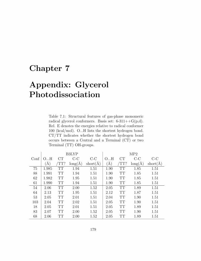
Chapter 7
Appendix: GlycerolPhotodissociation
Table 7.1: Structural features of gas-phase monomericradical glycerol conformers. Basis set: 6-311++G(p,d).Rel. E denotes the energies relative to radical conformer100 (kcal/mol). O...H lists the shortest hydrogen bond.CT/TT indicates whether the shortest hydrogen bondoccurs between a Central and a Terminal (CT) or twoTerminal (TT) OH-groups.
B3LYP MP2Conf O...H CT C-C C-C O...H CT C-C C-C
(A) /TT? long(A) short(A) (A) /TT? long(A) short(A)75 1.985 TT 1.94 1.51 1.90 TT 1.85 1.5188 1.991 TT 1.94 1.51 1.90 TT 1.85 1.5162 1.982 TT 1.95 1.51 1.90 TT 1.85 1.5161 1.990 TT 1.94 1.51 1.90 TT 1.85 1.5154 2.06 TT 2.00 1.52 2.05 TT 1.89 1.5164 2.13 TT 1.95 1.51 2.12 TT 1.87 1.5153 2.05 TT 2.01 1.51 2.04 TT 1.90 1.51103 2.04 TT 2.02 1.51 2.05 TT 1.90 1.5118 2.05 TT 2.01 1.51 2.05 TT 1.89 1.5183 2.07 TT 2.00 1.52 2.05 TT 1.90 1.5168 2.06 TT 2.00 1.52 2.05 TT 1.89 1.51
179
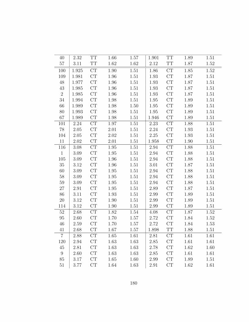
40 2.32 TT 1.66 1.57 1.901 TT 1.89 1.5157 3.11 TT 1.62 1.62 2.12 TT 1.87 1.52
100 1.925 CT 1.90 1.51 1.86 CT 1.85 1.52109 1.981 CT 1.96 1.51 1.93 CT 1.87 1.5148 1.977 CT 1.96 1.51 1.93 CT 1.87 1.5143 1.985 CT 1.96 1.51 1.93 CT 1.87 1.512 1.985 CT 1.96 1.51 1.93 CT 1.87 1.5134 1.994 CT 1.98 1.51 1.95 CT 1.89 1.5166 1.989 CT 1.98 1.50 1.95 CT 1.89 1.5180 1.993 CT 1.98 1.51 1.95 CT 1.89 1.5167 1.989 CT 1.98 1.51 1.946 CT 1.89 1.51101 2.24 CT 1.97 1.51 2.23 CT 1.88 1.5178 2.05 CT 2.01 1.51 2.24 CT 1.93 1.51104 2.05 CT 2.02 1.51 2.25 CT 1.93 1.5111 2.02 CT 2.01 1.51 1.958 CT 1.90 1.51116 3.08 CT 1.95 1.51 2.94 CT 1.88 1.511 3.09 CT 1.95 1.51 2.94 CT 1.88 1.51
105 3.09 CT 1.96 1.51 2.94 CT 1.88 1.5135 3.12 CT 1.96 1.51 3.01 CT 1.87 1.5160 3.09 CT 1.95 1.51 2.94 CT 1.88 1.5158 3.09 CT 1.95 1.51 2.94 CT 1.88 1.5159 3.09 CT 1.95 1.51 2.94 CT 1.88 1.5127 2.91 CT 1.95 1.51 2.89 CT 1.87 1.5186 3.11 CT 1.93 1.51 2.99 CT 1.89 1.5120 3.12 CT 1.90 1.51 2.99 CT 1.89 1.51114 3.12 CT 1.90 1.51 2.99 CT 1.89 1.5152 2.68 CT 1.82 1.54 4.08 CT 1.87 1.5295 2.60 CT 1.70 1.57 2.72 CT 1.84 1.5246 2.59 CT 1.70 1.57 2.72 CT 1.84 1.5341 2.68 CT 1.67 1.57 1.898 TT 1.88 1.517 2.88 CT 1.65 1.61 2.81 CT 1.61 1.61
120 2.94 CT 1.63 1.63 2.85 CT 1.61 1.6145 2.81 CT 1.63 1.63 2.78 CT 1.62 1.609 2.60 CT 1.63 1.63 2.85 CT 1.61 1.6185 3.17 CT 1.65 1.60 2.99 CT 1.89 1.5151 3.77 CT 1.64 1.63 2.91 CT 1.62 1.61
180
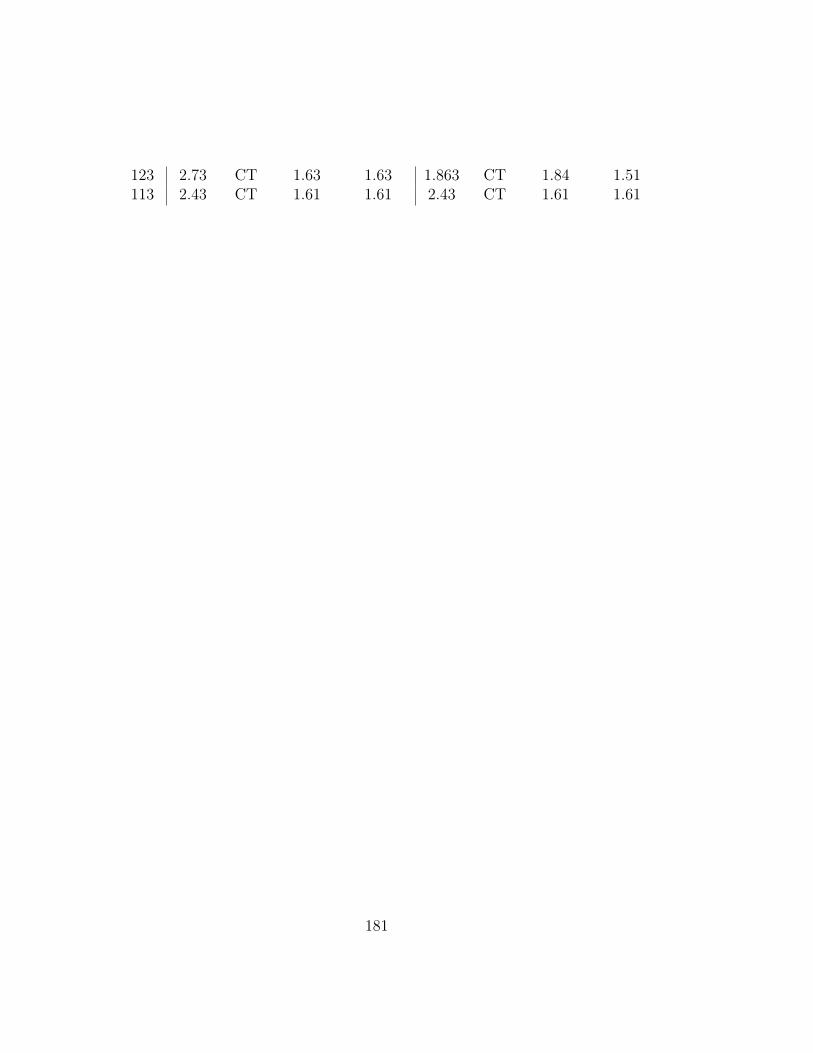
123 2.73 CT 1.63 1.63 1.863 CT 1.84 1.51113 2.43 CT 1.61 1.61 2.43 CT 1.61 1.61
181

Table 7.2: Relative energies (kcal/mol) for gas-phaseradical glycerol conformers. Geometries optimizedat the B3LYP/6-311++G(p,d) level of theory, exceptfor ωB97X(MP2), which were optimized with MP2/6-311++G(p,d). Unless stated, the basis set for the singlepoint calculations is 6-311++G(2df,2pd)
Conf B3LYP ωB97X ωB97X(MP2) MP2 MP2/aug-cc-pVTZ /T→Q extrap
75 0.41 0.19 0.45 0.3388 0.41 0.26 0.54 0.3362 0.41 0.17 0.41 0.2061 0.41 0.29 0.53 0.2254 2.48 2.14 2.07 2.2364 1.86 1.42 1.28 1.6753 2.53 2.19 2.14 2.28103 2.59 2.15 2.13 2.1918 2.60 2.17 2.09 2.3083 2.53 2.13 2.06 2.2468 2.58 2.22 2.14 2.2740 2.72 4.82 2.25 10.8057 7.27 10.73 1.39 8.18100 0.00 0.00 0.00 0.00 0.00109 -0.63 -0.88 -0.92 -0.57 -0.4048 -0.60 -0.79 -0.85 -0.60 -1.0343 -0.55 -0.78 -0.81 -0.58 -0.942 -0.55 -0.78 -0.81 -0.58 -0.9434 -0.76 -0.65 -0.62 -0.68 -1.1266 -0.71 -0.93 -0.92 -0.68 -1.1280 -0.71 -0.73 -0.73 -0.71 -1.1367 -0.71 -0.93 -0.92 -0.68 -1.12101 0.26 -0.28 -0.28 0.1378 0.32 0.18 0.28 0.51104 0.28 0.36 0.50 0.5611 0.47 0.41 0.38 0.68116 2.67 2.60 2.49 3.161 2.69 2.65 2.55 3.33
182
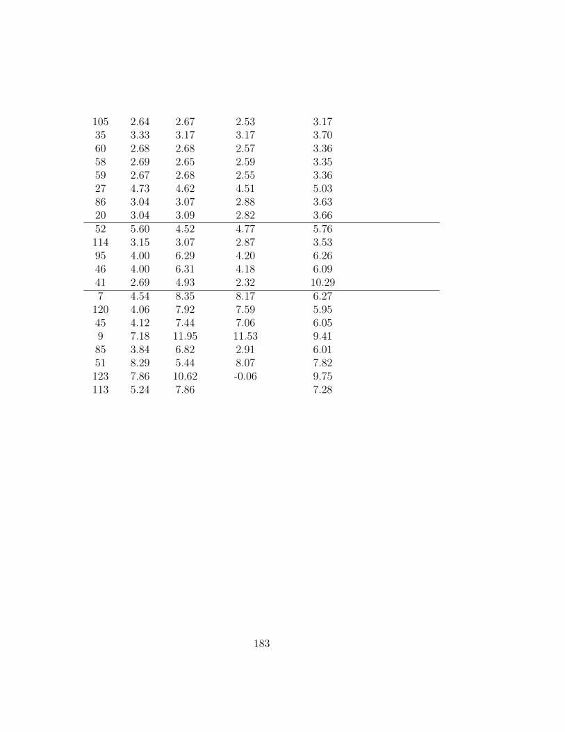
105 2.64 2.67 2.53 3.1735 3.33 3.17 3.17 3.7060 2.68 2.68 2.57 3.3658 2.69 2.65 2.59 3.3559 2.67 2.68 2.55 3.3627 4.73 4.62 4.51 5.0386 3.04 3.07 2.88 3.6320 3.04 3.09 2.82 3.6652 5.60 4.52 4.77 5.76114 3.15 3.07 2.87 3.5395 4.00 6.29 4.20 6.2646 4.00 6.31 4.18 6.0941 2.69 4.93 2.32 10.297 4.54 8.35 8.17 6.27
120 4.06 7.92 7.59 5.9545 4.12 7.44 7.06 6.059 7.18 11.95 11.53 9.4185 3.84 6.82 2.91 6.0151 8.29 5.44 8.07 7.82123 7.86 10.62 -0.06 9.75113 5.24 7.86 7.28
183