Rochester Institute of TechnologyRIT Scholar Works

Theses Thesis/Dissertation Collections

1974

Development and applications of a quadraticisoparametric finite element for axisymmetric stressand deflection analysisF. X. Janucik

Follow this and additional works at: http://scholarworks.rit.edu/theses

This Thesis is brought to you for free and open access by the Thesis/Dissertation Collections at RIT Scholar Works. It has been accepted for inclusionin Theses by an authorized administrator of RIT Scholar Works. For more information, please contact ritscholarworks@rit.edu.

Recommended CitationJanucik, F. X., "Development and applications of a quadratic isoparametric finite element for axisymmetric stress and deflectionanalysis" (1974). Thesis. Rochester Institute of Technology. Accessed from

DEVELOPMENT AND APPLICATIONS OF A QUADRATIC ISOPARAMETRIC

FINITE ELEMENT FOR AXISYMMETRIC STRESS AND DEFLECTION ANALYSIS

by

F. X. Janucik

A Thesis Submitted

in

Partial Fulfillment

of the

Requirements for the Degree of

MASTER OF SCIENCE

in

Mechanical Engineering

Approved by: Prof. Neville Rieger Thesis Advisor

Dr. Robert McCalley Jr. (External Reviewer)

Prof. B. Karlekar

Prof. Richard B. Hetnarski

Prof. Robert M Desmond (Department Head)

DEPARTMENT OF MECHANICAL ENGINEERING

ROCHESTER INSTITUTE OF TECHNOLOGY

ROCHESTER, NEW YORK

June, 1974

V

ACKNOWLEDGEMENTS

The author would like to express his appreciation to

those who have assisted him during the course of this in

vestigation and in particular:

To Professor N. F. Rieger, his thesis advisor, for his

interest and guidance of the author's thesis research and

for the profound effect that association with him has had

on the author's professional career.

To Dr. R. B. McCalley, Jr., external thesis examiner,

for his continued interest, insight, and encouragement in

the author's thesis research.

To Dr. J. F. Loeber and Mr. T. Glasser, Knolls Atomic

Power Laboratory, for their insight, suggestions, and

assistance concerning this investigation.

To Professors B. Karlekar, R. Hetnarski, W. Halbleib,

M. Sherman, and W. Walters, Rochester Institute of Technology,

Mechanical Engineering Department, for their interest, suggestions,

and encouragement concerning this thesis research.

To the author's wife Barbara for her encouragement

and patience.

To Mrs. B. Engle for her superior job in typing the

final manuscript of this investigation.

ABSTRACT

The theory and computer program for an axisymmetric

finite element for static stress and deflection analysis

is presented. The element is an eight noded isoparametric

quadrilateral based on the displacement method which is

capable of representing quadratic variation of element

boundaries and displacements. Element stiffness properties

are developed for linear elastic small displacement theory

using homogeneous isotropic material. Test cases are

compared with theoretical solutions from the theory of

elasticity to identify program capabilities and limitations .

Ability to analyse axisymmetric problems and to represent

curved element boundaries has been demonstrated. Example

problems including a cylindrical pressure vessel, a disk of

uniform thickness subjected to centrifugal body force, and

stress concentrations in a cylindrical rod due to a

spherical inclusion are presented. In each of these cases

program predicted deflection and stress values were within

2% of theoretical values .

Limitations which have been identified include the

prediction of discontinuous stresses at adjacent element

boundaries, failure to match original element boundary

stress conditions in substructure analyses, and the necess

ity of double precision calculations to correctly analyse

problems whose theoretical solutions obey small displace

ment plate theory. Analysis of a spherical pressure vessel

resulted in predicted displacements within 4% of theoretical

values while stresses on element boundaries varied by 60%

from theoretical values. Substructure analysis for the

spherical inclusion problem resulted in prediction of

boundary stresses which were incompatible with those

originally obtained. Techniques to overcome this difficulty

are proposed but are not tested. The inability to obtain

reasonable results for flexural problems was found to be

due to round off error in the single precision technique

used for solving the structure equilibrium relations. Use of

double precision calculations resulted in displacements and

stresses within .25% and 4.% respectively of theory for the

case of a clamped circular plate loaded by a uniform pressure

normal to its surface.

TABLE OF CONTENTS

PAGE

i List of Figures i

iii List of Tables iii

iv Nomenclature iv

1.0 INTRODUCTION 1

2.0 LITERATURE SURVEY 3

3.0 BASIC STEPS OF THE FINITE ELEMENT 7

DISPLACEMENT METHOD

4.0 DEVELOPMENT OF THE QUADRATIC AXISYMMETRIC 9

FINITE ELEMENT

4.1 Interpolation Formula and Isoparametric 9

Concept

4.2 Strain-Displacement Relations 17

4.3 Stress-Strain Relations 21

4.4 Force-Displacement Relations 23

4.5 Distribution of Element Loads to Nodal 27

Points

5.0 STRUCTURAL EQUILIBRIUM RELATIONS-THE STRUCTURAL30

STIFFNESS MATRIX

6.0 SOLUTION FOR STRUCTURAL NODAL POINT DISPLACEMENTS32

7.0 DETERMINATION OF ELEMENT STRESSES34

8.0 EXAMPLE PROBLEMS 39

8.1 Stresses and Deflections in a Cylindrical 40

Pressure vessel

PAGE

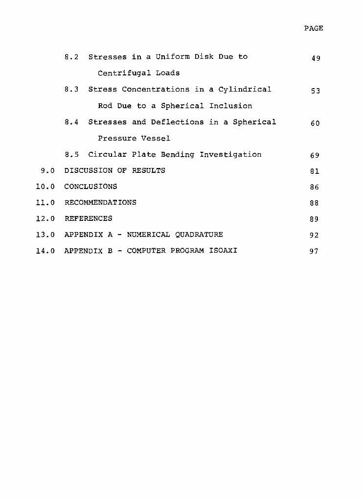
8.2 Stresses in a Uniform Disk Due to 49

Centrifugal Loads

8.3 Stress Concentrations in a Cylindrical 53

Rod Due to a Spherical Inclusion

8.4 Stresses and Deflections in a Spherical 60

Pressure Vessel

8.5 Circular Plate Bending Investigation 69

9.0 DISCUSSION OF RESULTS 81

10.0 CONCLUSIONS 86

11.0 RECOMMENDAT IONS 8 8

12.0 REFERENCES 89

13.0 APPENDIX A - NUMERICAL QUADRATURE 92

14.0 APPENDIX B - COMPUTER PROGRAM ISOAXI 97

LIST OF FIGURES

Figure Title Page

1 Element Mapping 11

2 Location of Element Nodal Points 12

3 Allocation of Surface and Body Forces for 29

a Regular Quadrilateral

4 A Banded Structural Stiffness Matrix 31

5 Quadrature Sampling Points and Element 38

Nodal Point Locations

6 Thick Cylindrical Pressure Vessel (TC 1) 42

7 TC 1 Finite Element Idealization 43

8 TC 1 Stress and Displacement Results 44

9 Uniformly Thick Disk Subjected to 51

Centrifugal Loading

10 TC 2 Radial and Hoop Stress Results 52

11 Cylindrical Rod With Spherical 56

Inclusion (TC 3)

12 TC 3 Finite Element Idealization of 57

Spherical Inclusion in Cylindrical Rod

13 TC 3 Variation of Axial Stress 59

14 TC 3 Refined Idealization 58

15 Spherical Pressure Vessel Subjected to 63

Internal Pressure (TC 4)

16 TC 4 Finite Element Idealization 64

17 TC 4 Volumetric Expansion Versus Radius 66

Figure Title Page

18 TC 4 Principal Hoop Stress Versus Radius 67

19 TC 4 Principal Radial Stress Versus Radius 68

20 Circular Plate Subjected to Uniform 77

Pressure-Problem and Idealization

21 Circular Plate Axial Deflection Results 78

22 Circular Plate Subjected to Uniform 79

Load - Radial Stress Versus Radius

23 Circular Plate Subjected to Uniform Load -

80

Hoop Stress Versus Radius

n

LIST OF TABLES

Table Title Page

I. Element Shape Functions 16

II. Midside Node Stress Matrices 38

III. TC 1 Summary of Results 47

IV. TC 4 Summary of Displacement Results 62

V. Abscissas and Weight Factors for 96

Gaussian Integration

VI. Comparison of Results of Thesis Versus Those of

Linear and Quadratic Triangular Elements 48

m

NOMENCLATURE

Scalars

r,z,6 Cylindrical coordinates (radial, axial,

circumferential )

P,Q Local normalized curvilinear coordinates

A Area

V Volume

u,v Displacement components in the radial and

axial directions respectively

F- ,F. Components of force acting in the radial and

axial directions respectively at nodal point i

e , eQ,e Normal components of strain in the r,9, z

directions

Yrz Shearing straxn in cylindrical coordinates

o ,Oc,ta Normal stress components in the r,8, z directionsi U 2

xrz Shearing stress in the rz plane

U Strain energy

E Young's modulus of elasticity

vPoisson'

s ratio

An arbitrary parameter varying within

an element (e.g. displacement, geometry)

<i>

4> . Value of unknown at element nodal point i

N. Element shape function associated with nodal

point i

a Unknown polynomial coefficient

IV

Vectors and Matrices

U

fn\

Row or column vector

[ ] Matrix

T T[ ] , | X Matrix or vector transposed

[ ] Inverse of a matrix

det[ ] Determinant of a matrix

\r \ Column vector of radial coordinates for

element nodal point s

jz 1 Column vector of element nodal point axial

coordinates

Column vector of element node radial dis

placement components

Column vector of element node axial dis

placement components

fW_l Column vector containing both radial and

axial displacement components of the

element nodes

[n p Row vector of element shape functions

ie ] Column vector of strain components

| a "I Column vector of stress components

[B] Matrix relating displacement to strain

[J] Jacobian matrix

[G] Matrix relating element nodal point locations

to the Jacobian matrix

[XQJ Matrix of element nodes spatial coordinates

[D] Matrix relating stress to strain

[K] Element stiffness matrix

Vectors and Matrices

|F y Column vector listing element nodal point

forces

|6Wj Column vector of virtual displacements in

radial and axial direction of an element's

nodal points

tBj Column vector of element body force components

\Pj Column vector of element surface force

components

[N*

] Matrix of shape functions

JA | Column vector of structure nodal point

displacement components

[K] Structural stiffness matrix

\r\ Column vector of structure nodal point force

components

[S] Matrix relating stress to displacement

vi

1.0 INTRODUCTION

All linear elastic static stress and deflection problems

of axially symmetric continua are, in theory, capable of

being solved using the finite element method. (e.g. pressure

vessels, cooling towers, rocket nozzles) . Limitations to

the finite element method occur when numerous elements are

required to achieve a desired degree of accuracy thus re

sulting in large computer core requirements and/or excessive

cost.

Prior to 1968, finite elements having only linear

variation of boundaries were available. Thus, when a

curved geometric boundary was to be modelled, one was forced

to introduce large numbers of elements to achieve acceptable

results. This required the solution of a greatly increased

number of equilibrium equations and was recognized as a

limiting factor in the application of the finite element

method to this type of problem.

Introduction of the isoparametric concept by Ergatoudis

[8] enabled development of elements with polynomic variation

of boundaries and led to a reduction in the number of ele

ments necessary to idealize curved boundaries.

The objective of this thesis is to present details of

an isoparametric finite element for axisymmetric stress

analysis which is capable of representing quadratic varia

tion of element boundaries exactly. The development of

the element, a computer program, and demonstrative applica

tions are presented.

The element developed is an eight-noded quadrilateral

based on the isoparametric element concept. Its material

properties are isotropic and linear. Element force-displace

ment relations are obtained using the displacement method

of minimum potential energy.

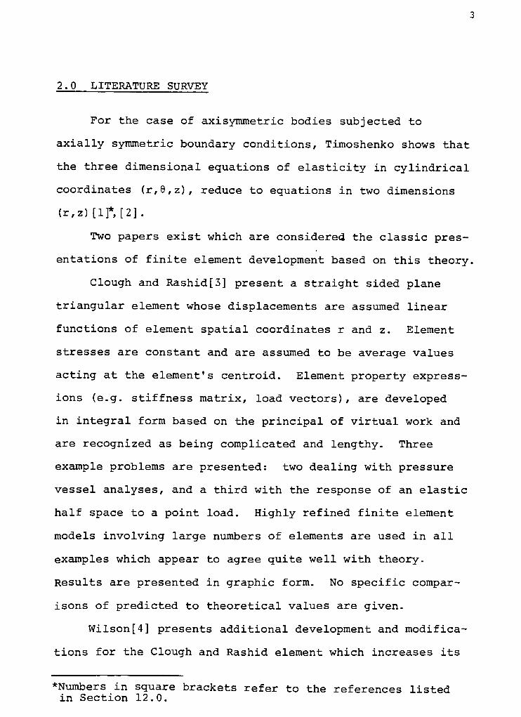
2.0 LITERATURE SURVEY

For the case of axisymmetric bodies subjected to

axially symmetric boundary conditions, Timoshenko shows that

the three dimensional equations of elasticity in cylindrical

coordinates (r,9,z), reduce to equations in two dimensions

(r,z)[l]*,[2].

Two papers exist which are considered the classic pres

entations of finite element development based on this theory.

Clough and Rashid[3] present a straight sided plane

triangular element whose displacements are assumed linear

functions of element spatial coordinates r and z. Element

stresses are constant and are assumed to be average values

acting at the element's centroid. Element property express

ions (e.g. stiffness matrix, load vectors) , are developed

in integral form based on the principal of virtual work and

are recognized as being complicated and lengthy. Three

example problems are presented: two dealing with pressure

vessel analyses, and a third with the response of an elastic

half space to a point load. Highly refined finite element

models involving large numbers of elements are used in all

examples which appear to agree quite well with theory.

Results are presented in graphic form. No specific compar

isons of predicted to theoretical values are given.

Wilson [4] presents additional development and modifica

tions for the Clough and Rashid element which increases its

?Numbers in square brackets refer to the references listedin Section 12.0.

ability to analyse a broader class of structural problems.

Presented is the development for determining steady state

thermal effects and a procedure for analysing axisymmetric

bodies experiencing asymetric loads. The technique for

the latter consists of introducing harmonic displacement

functions and summing a series of two dimensional analyses.

Wilson notes the advantage of quadrilateral elements for

automated mesh generation and presents development for a

quadrilateral element which is actually degenerated into

four linear displacement triangles. Factors which prohibit

direct formulation of quadrilateral elements are not con

sidered.

Superiority of the linear displacement trapezoidal

element over its triangular counterpart has been demosntrated

based on strain energy considerations by Parsons and Wilson

[32]. The internal work done by one trapezoid is shown to

be lower than that of two corresponding triangular elements

experiencing similar boundary conditions and the implication

is made that more and smaller triangular elements are necessary

to achieve results which are as accurate as those obtained

with quadrilaterals. Among the disadvantages discussed is

the difficulty to integrate for the stiffness matrix for

shapes other than trapezoidal and introduction ofinter-

element displacement incompatability when adjacent elements

are not rectangular.

1. For additional information, see Crose [5] or Ergatoudis [8]

The concept of an isoparametric element capable of over

coming the above disadvantages is credited to Taig by Irons [7]

and Ergatoudis [8] . The technique of introducing a local

curvilinear coordinate system is due to Taig[8] but was

also developed independently, including consideration of

curved element edge formulation and numerical integration

convergence criteria, by Irons[7].

Ergatoudis, working in collaboration "with Irons and

Zienkiewicz, was the first to present plane quadrilateral

elements based on the isoparametric concept [31] . Elements

for two dimensional stress analysis were developed assuming

linear, quadratic, and cubic boundary and displacement

variations. Numerous example problems were presented and

compared with solutions from the theory of elasticity- The

necessity of numerical integration is notedbut not discussed

in depth. Conclusions are drawn favoring isoparametric

quadrilateral elements having assumed variation functions

of higher than first order. Subsequent work by Ergatoudis [8]

includes the formulation of isoparametric, axisymmetric

quadrilaterals having quadratic, cubic, and quintic dis

placement and boundary variations. Example problems of

pressure vessels, circular plates, and rotating shafts in

which excellent results were obtained are presented.

justification for the choice of particular elements in

some examples is not provided.

The basic theory for deriving isoparametric elements

is available in numerous texts. Theory is presented by

Desai and Abel [17] and Martin and Carey [34] but the most

comprehensive treatment of the concept is presented by

Zienkiewicz [9]- [12].

Irons establishes the efficiency of numerical integra

tion [7] and presents efficient integration techniques for

the experienced analyst [13]- [15]. A recent paper by

Gupta and Mohraz[16] presents an efficient technique for

the numerical integration of element stiffness matrices

which may readily be placed in a programmable form. Also

included is a second technique which minimizes the number of

mathematical computations necessary and hence computer

time . A comparison of computer times between the two

shows the proposed technique to be more efficient.

Example problems which demonstrate the increased effic

iency cf higher ordered isoparametric elements are presented

by Dario and Bradley [21] for triangular elements and

Ergatoudis [ 8] , [31] for quadrilaterals.

3.0 BASIC STEPS OF THE FINITE ELEMENT DISPLACEMENT METHOD

Finite element development for stress and deflection

analysis may be based on either of two variational prin

ciples; i) principle of minimum potential energy or ii)

complementary energy theorem. The principle of minimum

potential energy states that the true deformations of a body

are those which make its potential energy a minimum. Ap

plication of this principle results in algebraic equations

of equilibrium. The complementary potential energy theorem

may be used to obtain algebraic equations of compatibility

The more commonly used principle is that of minimizing potential

energy since it facilitates assemblage of structural equil

ibrium relations. This technique is referred to as the

displacement method of finite element analysis .

Models comprised of finite elements based on the

displacement method tend to be stiffer than actual struc

tures . This fact is due to the restraint introduced in

prescribing intra-elementdisplacement variation. Refine

ment of idealizations or the use of higher order elements

minimizes this effect and provides convergence to true

displacement shapes .

The six basic steps of the finite element technique

based on the displacement method are:

1. Discretization of a continuum into an equivalent

system of finite elements which are interconnected

at nodal points .

2. Selection of a interpolation formula to approximate

the variation of displacement on and within element

boundaries .

3. Derivation of element stiffness matrices giving

equilibrium relations between the forces and dis

placements at each element nodal point.

4. Assembly of the element stiffness matrices based#

on nodal point force equilibrium and displacement

compatability to obtain structural equilibrium

relations.

5. Solution of the structural equilibrium relations

for unknown displacements .

6. Solution of element stresses based on element nodal

point displacements.

These steps are applicable for development of all finite

element types (e.g. plane stress/strain, axisymmetric, three

dimensional solid) . Development of a specific element type

requires further consideration of the governing elasticity

equations. The foregoing steps will now be applied to the

development of an isoparametric finite element for axisym

metric static stress analysis.

4.0 DEVELOPMENT OF THE QUADRATIC-AXISYMMETRIC FINITE ELEMENT

4.1 Interpolation Formula and Isoparametric Concept

The selection of an interpolation formula des

cribing the variation of some unknown i(e.g.

radial or axial displacement) within an element

is of foremost importance in developing a finite

element based on the displacement method. This

formula is generally expressed as:

n

(j) = E N. i>. (1)

i=lx x

where N. is a normalized "shapefunction"

of

polynomial form in spatial coordinates

<j>. is the value of the unknown function <J)

at element node i

n is the number of nodes used to define

the e lement

The shape functions in Eq, 1 may not be chosen

arbitrarily if monotonic convergence is to be

expected [10] . In order that finite element

solutions converge to true solutions, shape

functions must be chosen which:

1. Are of such order and form that continuity

of unknown <p occurs between elements.

2. Allow any arbitrary linear form of <j) to be

taken to represent constant derivatives.

With respect to element displacement, these require

ments imply that no gaps or overlapping of adjacent

10

element boundaries occur and that states of

constant strain may be represented.

Although the quadrilateral element has been shown

by Wilson and Parsons [32] to be superior to its

triangular counterpart, the use of cartesian poly

nomials to define element shape functions is not

suitable since convergence criteria can only be

satisfied for the limited cases of elements being

rectangles or parallelograms. The isoparametric

concept enables specification of shape functions

which will satisfy convergence criteria and

also allow arbitrary element shapes which are

consistent with assumed spatial variation. In

the isoparametric concept, element shape functions

are obtained for a square normalized element in

a local coordinate system (P,Q) . This coordinate

system has its origin at the centroid of the

element. Element boundaries have limits of -1

and 1 as shown in Fig. la. This normalized element

and its shape functions are then associated with

the curved element in spatial coordinates (r,z)

shown in Fig. lb. Therefore, coordinate system

(P,Q) becomes curvilinear and both curved element

displacement and geometry is expressed in terms of

P and Q through Eq. 1.

11

(-1, 1)

Q -

iO. 1),(1,D

(-It o)

l7

'

( 1, 0)

(-1,-1) , i

'p

( 1,-1)(0,-1)

a) local coordinate system

(r,z)

b) global coordinate system

Element Mapping

FIGURE 1

12

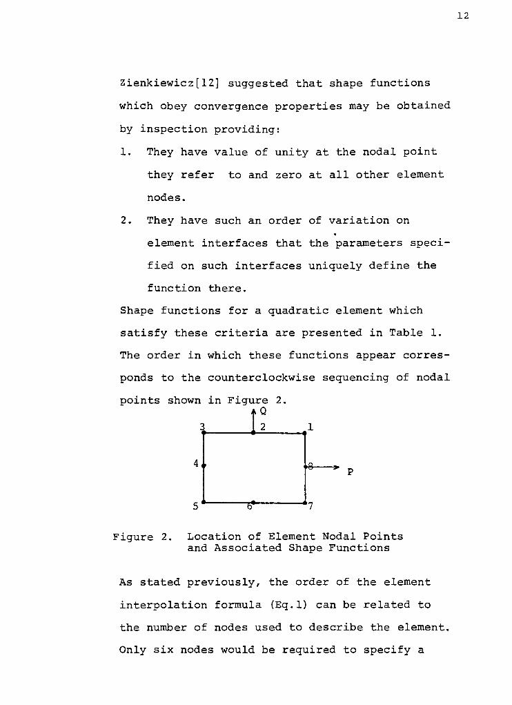
Zienkiewicz [12] suggested that shape functions

which obey convergence properties may be obtained

by inspection providing:

1. They have value of unity at the nodal point

they refer to and zero at all other element

nodes.

2. They have such an order of variation on

element interfaces that the parameters speci

fied on such interfaces uniquely define the

function there.

Shape functions for a quadratic element which

satisfy these criteria are presented in Table 1.

The order in which these functions appear corres

ponds to the counterclockwise sequencing of nodal

points shown in Figure 2.

? Q

Figure 2. Location of Element Nodal Points

and Associated Shape Functions

As stated previously, the order of the element

interpolation formula (Eq.l) can be related to

the number of nodes used to describe the element.

Only six nodes would be required to specify a

13

complete quadratic function in two variables. To

maintain symmetry of the element, eight nodes are

used. Expansion of Eq. 1 in terms of P and Q,

using the above shape functions, the interpola

tion formula will be found to contain two terms

2 2of cubic order, PQ and P Q. Therefore, although

the element is referred to as quadratic, actual

element variations are assumed which are higher

order.

The axisymmetric problem in cylindrical coordinates

may be completely specified in two dimensions.

When axisymmetric boundary conditions exist, strain

relations are completely specified in radial and

axial coordinates (r,z), independant of 9. Thus,

only two-dimensional finite elements in the r-z

plane need be considered.

From Eq. 1, the variation of displacement within

an element may be expressed as:

u = [N] un] (2)

v = [N] ^vn} (3)

where u and v are radial and axial displacement

components respectively at any point within the

element.

14

[N]is a matrix of element shape functions:

[N] =

[Nr N2, N3, Ng]

lUnI 1 v \ are clumn vectors of element nodal point

displacement components.

KlT

= [UV n2' u3' ' '

usl

{\Y = Jvl' V2' V3' * vs}'

By definition, element geometry is also defined by

Eq. 1 and may be expressed as:

r = [N] \rn] (4)

z = [N] [z^ (5)

where r and z are element spatial coordinates in the

radial and axial directions, jr | , jz r are

column vectors of element nodal point coordinates .

{rnf = [rl> r2' r3' ' '

r8^i

lZni=1Z1' Z2' Z3' * '

*Z8}

To demonstrate the element's ability to represent

quadratic varying boundaries, consider Eqs. 4 and

5 for the case P = 1 which corresponds to the

element edge defined by nodes 1, 7, and 8 in

Fig. 2. From Table 1, shape functions N_

15

through Ng are zero and Eqs. 4 and 5 simplify to:

r =

r8+

H(r1-

r?)Q + h (r+r?

-

2rg)Q2

z =

z8+

h(z-

z?)Q +h(Zl

+z?

-

2zg)Q2

which represents a quadratic variation of element

boundary .

These element displacement and geometry relations

will now be used to establish element strain and

stiffness properties.

16

TABLE I

ELEMENT SHAPE FUNCTIONS

iN.l

3N.l

dp,

3N.l

3Q

1 %(1+P) (1+Q) (-1+P+Q) kU+Q) (2P+Q) ^(1+P) (2Q+P)

2 Ml-P2) (1+Q) -P(l+Q) %(1-P2)

3 %(1-P) (1+Q) (-1-P+Q) !*(1+Q) (2P-Q) %(1-P) (2Q-P)

4 ^(1-P) (1-Q2) -h d-Q2) -Q(l-P)

5 %(1-P) (1-Q) (-1-P-Q) ^(1-Q()2P+Q) h(l-Q) (2Q+P)

6 %(1-P2) (1-Q) -P(l-Q) -^(1-P2)

7 Ml+P) (1-Q) (-1+P-Q) %(1-Q) (2P-Q) %(1+P) (2Q-P)

8 -5(1+P) (1-Q2) Ml-Q2) -Q(l+P)

17

4.2 Strain-Displacement Relationships

As developed by Timoshenko [1 J, the linear strain-

displacement relations for an axisymmetric body

experiencing axisymmetric boundary conditions

reduce to the following in cylindrical coordinates

= iHer

"

3r

u

e9=

r

e =

Z 3z

3v(6>

y 3u+

3v

rz

""

3z 3r

where u and v are displacement components in the

radial and axial directions respectively.

Substituting Eqs. 2 and 3 into Eq. 6, the element

strain may be expressed in matrix form as:

H-

W\"o] (7)

where {=

^ eQ ez Yrz ]

[B] =

[B]_ B2 B3 . . . Bg]

18

[B.] -3Ni

N.l

0

~N.

3 l

3z

3 l 3 l

3z 3r

and^Wo}T

=

^ V;L u2 v2. . .

u8 Vg]

The coefficients of matrix [LB] contain derivatives of

the element shape functions with respect to cylindrical

coordinates. The shape functions are defined in terms

of normalized coordinates (P,Q) .

A relationship may be established between derivatives of

two coordinate systems by the introduction of the

Jacobian matrix of transformation from (r,z) to (P,Q)

[23] .

Applying the chain rule and differentiating shape

function N. with respect to P or Q, one obtains:

N N Ni

_

3 l 3r ,3 l 3z

3P'

3r 3P 3z 3P

.N.

3 l

3Q

3^i 3r

3r 3Q

3Ni 3z

3z 3Q

19

or in matrix form:

r

<

3Ni

3P

3 1

3Q

> =

3r

^P

3r

3Q

3z

3P

3z

3Q

<

d_h

3r

3 l

3z

y

where the matrix

3r 3z

3P 3P

3r 3Z

3Q 3Q

= [Jl

is called the Jacobian matrix.

Premultiplying both sides of the above equation

by the inverse of the Jacobian, derivatives of the

shape functions with respect to cylindrical coor

dinates may be expressed as:

= [J]-1

3 l

3P

3 l

3Q

>

Determination of the Jacobian matrix is accomplished

by differentiation of Eqs. 4 and 5 with respect to

P and Q.

20

Applying the chain rule, the four coefficients of

the Jacobian matrix become:

8 3N, _ 8il3P I

i = l

8

3r =

3QZ

i=l

3N.l

3P

JH.3 l

3Q

ri;

ri;

3_z

3P

3N.

il3Q

E

i = l

8

= Z

3P

dN

Z.l

z.1

i=l 3 Qsince the spatial coordinates of element nodes are

constant.

These relations may be written in matrix form as:

[J] =

[G] [XQ]

where

[G] =

3N1 ,

3P

3N2,3P

3 3, . . . ,

3P

3N8

3P

-Nl,

3Q

3N2f

3Q

3N3

3Q

3N8

3Q

[x0]T

rl r2 r3* * '

rV

Jl Z2 z3* * *

Z8_

21

4.3 Stress-Strain Relations

Element stress-strain relations are presented for

homogeneous, isotropic material.

For axially symmetric bodies, four components of

stress exist. Normal stress components are in

the axial, radial, and circumferential directions

and shearing stress exists in the r z plane.

In the absence of initial strain, the relations

between these element stresses and the element

strains are:

ar =E(l-v)

er+ (----) (efl + ej

(1+v) (1-2V)r

l-vz

a9=

(l+v)U-2v) e9+

(T-V (ez+ er)

az=

(WH1-2V) ez+ (T=v> (er

+ e9)

Y,rz 2(l+v) 'rz

where E represents Young's modulus

v represents Poisson 's ratio

These relations may then be expressed in matrix

form as:

^a}= [D] ^e] (9)

where

22

{II aa

a t

9. z rz 1

[D] =E(l-V)

(1+v) (l-2v)

V

V

<v> <)

V

<>

(iz2v

)

23

4.4 Force - Displacement Relations

Relations between element nodal point forces and

displacements may be obtained by the use of Cast

igliano's theorem. The strain energy of an axis

ymmetric element in a general state of stress may

be expressed in matrix form as:

0-1/2 IWT

[-} dV U0)

V

From Eqs. 7 and 9,

{e}= [B] {%}

[a}= [D] \e] = [D] [B] [uo]

The volume integral in Eq. 10 is expressed in

cylindrical coordinates as:

J dV = iff rd9drdz = ( C 27rrdrdz

v z r o z r

From Eq. 4.

r = [N] ^rQ}

Thus

J dV = J J 2tt [N] [rQ^ drd:

V z r

Substituting the above relations into Eq. 10, the

strain energy may be written as:

U =

J'ItT[wo\T[B]T[D][B]^Wo"\[N]^ro]

drdz (11)

z r

24

Using the above relation andCastigliano'

s Theorem,

the equilibrium relations between nodal point forces

and displacements may be found.

Castigliano*

s Theorem states, "If the strain energy

U of an elastic element is represented as a function

of statically independant displacements, the partial

derivative of this function with respect to displace

ments will give the actual forces at the displaced

points in the directions of thedisplacements"

. [1]

Or

where (f i refers to nodal point force components

of an element.

{FoY ={Flx' Flz' F2r' F2z' ' ' ' F8r' F8z}

Applying the above to Eq. 11 we obtain,

\Fo}=

<J J 2tt[B]T[D][B][N] [r^\ drdz > {\*o\

or

i*0)- wD

where

[K] = J J 2tt[B]T[D][B][N] (rl drdz (12)z r

25

and is the element stiffness matrix.

Evaluation of element stiffness by direct inte

gration of Eq. 12 is not practical. Matrices [Bj and

[N]are expressed in curvilinear coordinates and

would require transformation to cylindrical coord

inates. Also, limits of integration are complicated

by the curved boundaries shown in Fig. lb.

These difficulties are overcome by transforming Eq.

12 to an integral in the local normalized coordinate

system shown in Fig. la. This transformation is

accomplished by recognizing that the determinant

of the Jacobian matrix is equal to the ratio of

differential areas in global (drdz) and local

(dPdQ) coordinates [23].

drdz = det[J]dPdQ

Applying this relation to Eq. 12 and changing limits

of integration, the element stiffness matrix may

be expressed as:

1 1

[K>J J 2TT[B]T[D][B][NUr \ det[J] dPdQ (13)

-1 -1

^ OJ

where all quantities within the integral are either

constants or functions of P and Q.

Although limits of integration have been simplified,

the quadratic form of the shape functions result

26

in an expression to be integrated which is complex

in form and not practical to integrate analytically,

For this reason, evaluation of Eq. 13 is most

readily accomplished by numerical integration using

the Gauss quadrature technique. Details of the

procedure used herein are presented in Appendix A.

27

4.5 Distribution of Element Loads to Nodal Points

In the finite element method, structural loading

conditions are represented as point loads applied

at the nodes of the idealized structure. In cases

where distributed surface and body forces are

present, these forces may be"intuitively"

dis

tributed to the nodal points, or a specific

routine may be used.

In the case of higher order elements there is a

departure from an easily conceived idealization

and the allocation of distributed loads to nodal

points by intuition may no longer be correct, [12] .

However, nodal point loads, consistent with the

assumed displacement functions, may be formulated

for distributed loads by considering the Principal

of Virtual Work, viz:

"If an element which is in equilibrium under a

set of body forces ()BV) and surface forces (|PM ,

is given an arbitrary virtual displacement i 5w [,

which does not violate kinematic and geometrical

boundary constraints, then the work done by the

internal forces equals the work done by the applied

loads during these displacements,"

[19] .

This statement leads to the matrix equation:

J W}T^pl dA + J {sw}T|b$ dV={<SWq^ T[f^ (17)

28

where

dA = differential surface area of an element

boundary

dV = differential volume within the element

(jSW-J= virtual displacements of the element's nodes

^5WJ= virtual displacements within the element

Note also that ^5w]= [N1

] JfiwA from assumed variation

of intraelement displacement.

[N] =Nx o

N2 o N o . . . Ng o

ON1

ON2 o N_ . . . o Ng

F = force components at element nodal points

As ^5W^T

= (<5wl T[N' ]T

Eq. 17 becomes:

^ [N']T[p JdA + J[N']T|BJdV = [f] (18)V

The increased flexibility introduced in defining

element shapes in cylindrical coordinates compli

cated the limits of integration in Eq. 18. It

is found convenient to transform these integrals

to the local coordinate system and integrate

numerically as was done with the element stiffness

matrix.

The option to internally generate these consistent

loads has not been developed in the program

presented, but, wherever required, allocation of

distributed loads has been made as shown in Fig. 3.

29

.r M \t M ]! if ir u

Bo

I 1 1

Pq= surface force

Bn= body force

a) distributed loads on element

1/6 P,

b) equivalent surface forces

-1/12 BQ .-1/3 BQ

1/3 BQ

-m-

!

-1/12 BQ

<? 1/3 B,

l/3 B

.1/12 Bn +4 : -

' ' ^ "1/12

Bnuc) equivalent body forces

Allocation of Surface and Body Forces

Por a Regular Quadrilateral

Figure 3

30

5.0 STRUCTURAL EQUILIBRIUM RELATIONS-THE STRUCTURAL STIFFNESS

MATRIX

For the previously developed element stiffness matrix

[K] ,equilibrium equations relating element nodal point

forces to displacements were obtained.

The next step of the displacement method is the deter

mination of equilibrium relations between nodal point

forces and displacements for the entire structure or,

the structural stiffness matrix [K] .

The almost universally employed technique for obtaining

this matrix is the direct stiffness method [17] which

involves assembling the individual element stiffness

matrices such that both displacement compatability and

force equilibrium are satisfied at the nodal points,

as follows:

1. All elements adjacent to a particular node must

have the same displacement components at that node.

2. The external forces acting at a nodal point must

equal the sum of the internal forces contributed

by the elements meeting at the node.

Using these criteria, the structural stiffness matrix

[K]S

may be obtained by direct addition of the indivi

dualelements'

stiffness coefficients to their appropri-

ate locations in [K] .

31

These appropriate locations are determined by the nodal

points defining each element.

Two important properties which the structural stiffness

matrix possesses are

1. For linear elastic systems the element stiffness

matrix is symmetric (i.e. [K] = [K]TJ and the

assembled structural stiffness matrix is also symmetric,

2. Seauencing of elements and nodal points

such that the maximum difference between nodal point

numbers defining an element is a minimum, the result

ing structural stiffness matrix will be banded as

shown in Fig. 4.

Proof of these properties may be found in either reference

[12] or [17].

Although these properties may not appear significant,

they play an important role in an efficient scheme for

solution of the structural equilibrium equations which

requires a minimum amount of computer core capacity.

[K]'

xxxooooooo

xxxxoooooo

xxxxxooooo

oxxxxxoooo

ooxxxxxooo

oooxxxxxoo

ooooxxxxxo

oooooxxxxx

OOOOO 0 XX XX

Figure 4

A Banded Structural Stiffness Matrix (x = non-zero terms)

32

6.0 SOLUTION FOR STRUCTURAL NODAL POINT DISPLACEMENTS

Having found the structural stiffness matrix [K]s,

the structural equilibrium relations may be written as

^RJ=

[K]S

^AJ (19)

where \Rl= a vector of external force components

acting at the nodes of the structure

h\= a vector of displacement componets of

the nodal points of the structure

w

The external forces applied at nodal points may be added

directly to their appropriate locations in vector \ R r .

Also required is a sufficient number of prescribed

displacement components in the vector jA f to prevent

rigid body motion of the structure. Failure to constrain

rigid body motions will result in matrix [K ] being

singular and not possessing an inverse.

Introduction of prescribed displacements to Eq. 19 is

accomplished by modification of Uf and [K] such that

vector \ A \ will remain a vector of unknowns but yield

the correct prescribed displacements when solved.

Having defined vector |R^ and introduced prescribed

displacements, Eq. 19 may be solved.

Computer subroutines for the assemblage of the structural

stiffness matrix and solving structure equilibrium

equations were taken from an existing finite

33

element computer program developed at the General

Electric Research and Development Center by Levy [20]

and used with only minor modifications for accomodation

of the element developed.

Although no documentation of the above techniques is

available in this report, the procedures used are

similar to those presented by Cheung and King. [12].

The specific numerical technique used in finding dis

placements is a direct solution method using Gauss

elimination for a tridiagonal matrix whose coefficients

are themselves matrices.

Advantage of this technique is that a minimal amount of

computer core required as all zero coefficients outside

the bandwidth need not be retained. However, frequent

accesses to peripheral storage devices during the Gauss

elimination tends to increase total computer time.

As a result of the minimizing of core requirements

possible using this technique, the computer program given

in this thesis is capable of handling 600 nodes or 1200

displacement degrees of freedom. Such a problem corres

pondsto[K]S

being of the order 1200x1200 and would

require 1.44 x 10 words of computer storage with full

retention of the structural stiffness matrix. The computer

core required for the solution of this problem using the

tridiagonal method is 10,100 words.

34

7.0 DETERMINATION OF ELEMENT STRESSES

Having determined nodal point displacements, it is then

desirable to find stress components within the structure,

Structural stress components are determined on aper-

element basis and may be determined by a number of

different techniques.

Three techniques currently used for obtaining element

stress components, are:

1. Calculating stress components at element centroids

and assuming these to be the average values of

stress within each element. [17]

2. Assuming a polynomial variation of stress components

and extrapolating these components to element

boundaries. [20]

3. Calculation of consistent stress distributions based

on the theory of conjugate approximations, [24] ,[25].

Of these three techniques, the second has been employed.

The first technique was found to be too limited in

stress information available while the third required

sophistication beyond the scope of this thesis.

An advantage of the second technique is its ability to

determine stresses on element boundaries, (where mag

nitudes are often a maximum) with a minimum of effort.

Its disadvantage is that values of stress components

calculated at a point similar to adjacent elements may

35

exhibit finite discontinuities between the elements.

This is demonstrated in section 8.4.

From Eq. 7, the matrix expression:

)e\ = [B] U 1U J V cj J

was obtained which related element strain to its nodes'

displacements .

From Eq. 9, the element stress vector was expressed as:

I - w IThe relationship between stress and displacement is then:

[o]= [D][B] ^W^

where the matrix product [D ] [B ] is often referred to as

the stress matrix [S] .

Stress components may be found at the midside nodes of

each element by considering the element in its local

normalizing coordinates.

As shown in Appendix A, the product [D] [B] is found at

nine sampling points within an element when determining

element stiffness. The locations of these sampling

points are shown ih Figure 5.

Since the locations and stress matrices of the sampling

points are known, it is possible to extrapolate these

matrices to the element's midside nodes.

Consider Fig. 5 for the case of P = 0. By definition,

element nodes 2 and 6 lie on this line, and also sampling

36

points 4, 5, and 6.

Assuming quadratic variation of the stress matrix as

a function of Q, the stress matric [S (Q) ] may be

written as:

[S(Q) ]= a1+ a2Q +

a3Q2

where a,, a-, and a.- are unknown coefficients to be

determined.

The stress matrices at nodes 2 and 6 become:

[S] node 2 = a, +

a?+ a.

[S] node 6 =

ax+

a2+ a.

Denoting [S]. and a. as the stress matrix and coordinate

Q of sampling point i respectively, the following three

equations are obtained.

[S]4= a1+

a4a2+ a

4 ^

2[S]_ = a. + a_a. + a -,

<*

5- T

^5^2T d

5 ~3

2

5a2+ a

6a3

r ,2

[S]- + a, + aca0 + a fict

The above represents 3 equations having 3 unknowns and

may be solved forou , a_, and a_.

Using the same procedure for the case Q = 0, stress

matrices at nodes 4 and 8 may be obtained in terms of

the stress matrices at sampling points 2, 5, and 8.

37

Relationships between element midside node stress matrices

and the stress matrices at the sampling points are pre

sented in Table II.

38

Figure 5. Quadrature SamplingPoints*

and Element

Nodal Point Locations

TABLE II

Midside Node Stress Matrices

[S ] node 2

[S ] node 6

[S ] node 4

[S ] node 8

0.1878 [S]4

1.4788 [S]4

1.4788 [S]2

0.1878 [S]2

.6666 [S]5+ 1.4788 [S]6

.6666 [S]5+ 0.1878 [S ]6

.6666 [S]5+ 0.1878 [S]g

.6666 [S]5+ 1.4788 [S]g

39

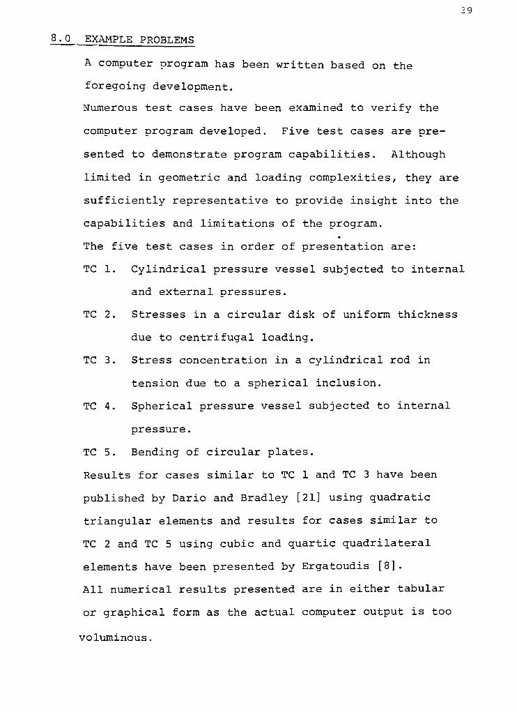
8 0 EXAMPLE PROBLEMS

A computer program has been written based on the

foregoing development.

Numerous test cases have been examined to verify the

computer program developed. Five test cases are pre

sented to demonstrate program capabilities. Although

limited in geometric and loading complexities, they are

sufficiently representative to provide insight into the

capabilities and limitations of the program.

The five test cases in order of presentation are:

TC 1. Cylindrical pressure vessel subjected to internal

and external pressures.

TC 2. Stresses in a circular disk of uniform thickness

due to centrifugal loading.

TC 3. Stress concentration in a cylindrical rod in

tension due to a spherical inclusion.

TC 4. Spherical pressure vessel subjected to internal

pressure.

TC 5. Bending of circular plates.

Results for cases similar to TC 1 and TC 3 have been

published by Dario and Bradley [21] using quadratic

triangular elements and results for cases similar to

TC 2 and TC 5 using cubic and quartic quadrilateral

elements have been presented by Ergatoudis [8] .

All numerical results presented are in either tabular

or graphical form as the actual computer output is too

voluminous .

40

8.1 STRESSES AND DEFLECTIONS IN A CYLINDRICAL PRESSURE

VESSEL TC 1

This case is presented to verify the ability of the program

to solve axisymmetric problems and involves the class

ical thick cylinder problem from the theory of elasticity -

The theoretical solution of this problem is due to Lame

and is presented by Timoshenko [1] . Cylinder geometry

and loading is presented in Fig. 6. Of primary interest

is radial stress, hoop stress, and radial displacement.

The theoretical displacement solution contains 1/r

2terms and stresses terms involving 1/r .

Refinement of finite element models is necessary to

approximate true stresses and displacements since actual

variations are of higher order than those assumed within

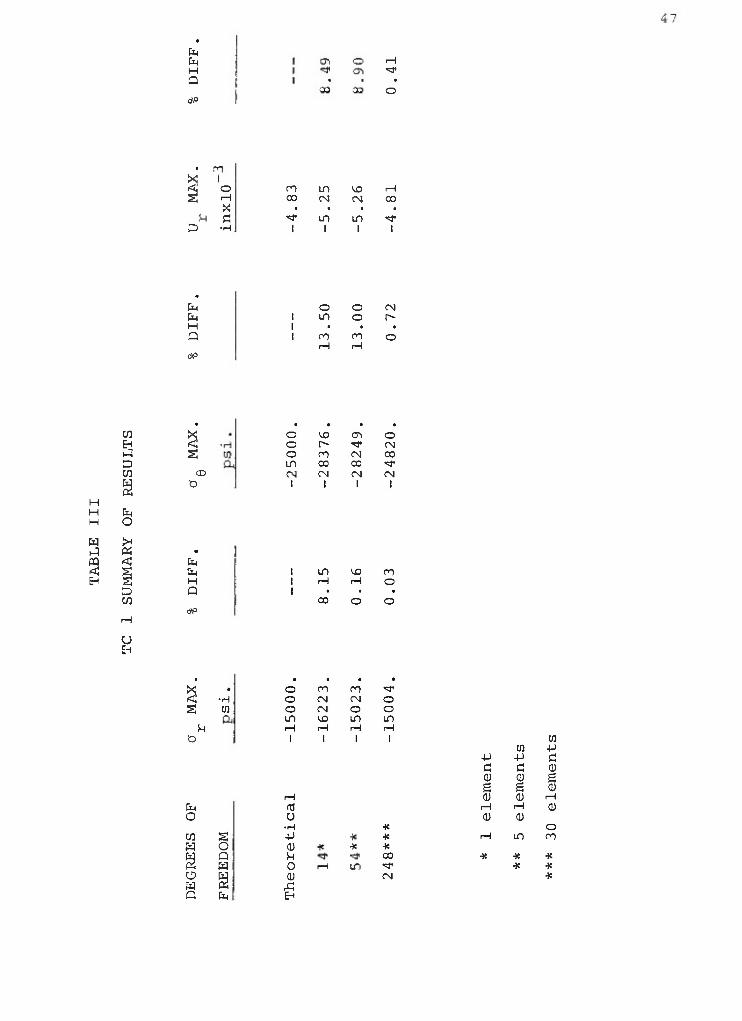
an element. Three finite element idealizations are

presented having 1, 5, and 30 elements respectively.

These models are shown in Fig. 7 and their results

summarized in Table III. Graphs of radial stress, hoop

stress, and radial displacement are presented in Fig. 8

for the 5 and 30 element models comparing their results

with theory. For the 30 element model, stresses and

deflections have converged to within a maximum difference

of 1.0% of theoretical values at all locations.

Comparison information for the problem shown in Fig. 6

is available in a paper by Dario and Bradley [21] A

41

comparison between predicted stresses for the quadratic

quadrilateral and linear and quadratic triangles is

presented in Table VI, displacement information is not

available. Superiority of the quadratic quadrilateral

over the linear triangle is apparent. Advantage over its

triangular counterpart is not as evident.

An unexpected result of this analysis was the prediction

of displacements converging to the true solution from an

upper bound. This contradicts the fact that elements

based on the displacement method always prove too stiff.

Two exceptions to this rule occur when either interelement

displacement compatibility is not maintained or when

element volume integration is approximate. Neither of

these exceptions are believed to apply in this develop

ment. Also, similar displacement results were not

obtained in other example problems.Explanation

0f

this result is not available.

Results demonstrate functioning of the thesis program

and also that the accuracy is a function of model re

finement.

42

<-

rQ= 10. in.

r .

i

= 5 .irrr

Pi= 9000. psi, E = 3Q.xlO psi

Y= 0.30

axis of symmetry

PQ= 1500*?. ps:

H = 1.0 i:

FIGURE 6

?hick Cylindrical Pressure Vessel

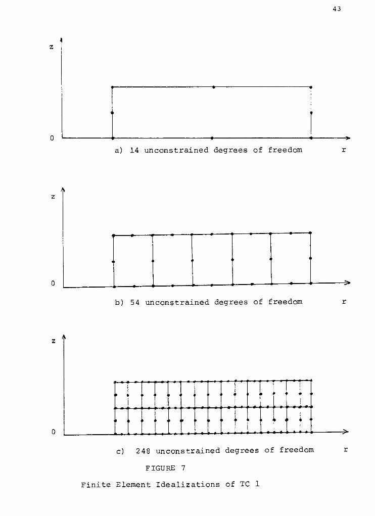
43

a) 14 unconstrained degrees of freedom

b) 5 4 unconstrained degrees of freedom

i\

|.

-

. . r .-

f|

' f'

T'

T'

f'

1' "

c) 2 48 unconstrained degrees of freedom r

FIGURE 7

Finite Element Idealizations of TC 1

47

Uj

UjH

Q

o\o

5T

CO

O

cn

00

a

1

o ro IT) CD rH

H CO CN CN 00

X .

a ^ in cn -r

H 1 I 1 I

Em

UjH

Q

o

m

n

o

o

CM

CO >SEH <J aD

W c

O

H

H EmH o

w >H

JPQ < Ed

<En |

EnH

D Q

Cfl

dP

rH

uEh

CD

H

CO

Si

o ^D CTl O

o r- "3<CN

o niT-

CO

in CO CO *

CN

l

CN

1

CN

1

CN

1

in

CO

VD cn

o

H

tn

o 00 cn *

o CN CN o

o CN O o

in CD m in

rH

i

r-i

1

t-i

I

H

I

Em cd

O 0

H *

Ui a +J * *

Ui o OJ * * *

3Q H -r ^r 00

W 0 .H in -*

o H OJ CN

a s XJQ Em Eh

tn 4->

-P -p Cl

C c OJ

<D 0) gg g (I)

<u <D H

H H OJ

<D 0)

o

H in m

* * *

X

*

48

co

H

Ui

Ui

XEh

ft!

P

CUP ura ri

H -P

H fd

P, M

TS T3

cd (C

3 3C O1

c\ 0V3

ro CN

o or-

oo

H

>

CQ

<Eh

Em

O

>H

W

oXEh

Q u

CflEh 3

a)rH

H

-P

3 CQ tr id

Etl c p 0\P

a 3 cd Xi VO dp

DCfl

w H rn in o -tf rH

q o iH 3 o *

E=q H

tfP C H o O

oi

Ui

>

cs;

a

Ui

H

Cfl

Ui

XEh

Du

H

tf >H

JH EJ

Em

OU

H

a

Q<u

Eh rH

CflEh

DCfl

patf

< P3 tn Sh

tf fl id HP

Q -3 cd 0) ro d*>

< H c in o -r r-

D o Sh ri o VD

O H

tf-P rH rH rH VD o

Em

O

Q

<Q

cn

OCfl

H

<PLA

aou

tf<

>

0)

o

fl

2 fl uH 0 <D1-q H

.. 4H

-P U) 4H

0 c -P H

fl 0 fl T3

3 H cn SJt <4H -p (U g CO ..

cu cd O CU en cn

Qj -P 0 H (U cn #

cd c H fl CU !h CU cn

-fl CD 0 P u cn

cn g UH MH MH cn P cu

cu fl 0 0 cn M

P o H g -P

fi cd SH U 3 r-l

cn

cu rH H (IJ d) g cd

gcu

<UT) g g

H

X

HQ-

0H H 0 3 3 id cd 0

w a a a-J 2 a tf X

49

8.2 Stresses in a Uniformly Thick Disk Due to

Centrifugal Load TC 2

The second test case is a classic problem in the

theory of elasticity and involves the determination

of radial and hoop stresses in a circular disk of

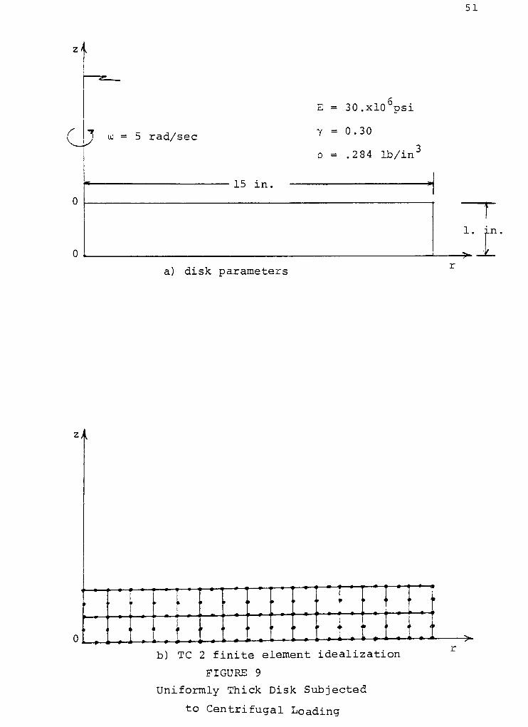
uniform thickness subjected to centrifugal loading.

Problem geometry and loading conditions are shown

in Fig. 9a. The finite element model used contained

30 elements and 125 nodes and is shown in Fig. 9b.

Theoretical solutions for stresses are presented by

Timoshenko [1 ] and are quadratic in nature.

Results from the finite element idealization are

compared with their theoretical values in Fig. 10

and for all practical purposes may be considered

exact.

Consideration in this analysis was not only deter

mination of accurate stress values but also the

work necessary in specifying the body force load

ing condition.

Body forces were calculated for each element and

specified as external forces acting at the model

nodal points, consistent with the allocation scheme

shown in Fig. 3.

Using the above technique presents severe limita

tions in representing this type of problem which

50

include:

1. An excessive amount of time to calculate element

body forces and distribute them to the nodal

points.

2. A necessarily large amount of input data for

specification for the external nodal point

forces calculated.

3. In the case of elements with curved boundaries,

allocation of element body force to its nodes is

no longer obvious as in the case presented and

requires additional consideration.

All of the above limitations may be alleviated by

the introduction of a subroutine in the program to

internally calculate and distribute body forces to

nodal points on a per element basis. Also, the

third limitation cited is greatly reduced by using

quadrature techniques. The computer program devel

oped does not contain this option which is left

for future development.

51

zK

C 1 co = 5 rad/sec

Z/l

E = 30.xl0 psi

Y = 0.30

p =.284

lb/in"

15 in H

a) disk parameters

a a a a,i a a .

r

. ,. <r ,

niUl ">-

b) TC 2 finite element idealization

FIGURE 9

Uniformly Thick Disk Subjected

to Centrifugal Loading

52

53

8.3 Stress Concentrations in a Cylindrical Rod Due to

a Spherical Inclusion TC 3

The problem of axial stress concentration in a cylin

drical rod containing a spherical inclusion was

analysed as a test case to demonstrate the program's

ability to represent curved boundaries and predict

stress concentration values. The. rod is subjected

to a uniform tensile stress distribution as shown

in Fig. 11.

The actual problem follows the notation of Dario

and Bradley [21 J. A closed form solution is presented

by Timoshenko [ 1] .

The finite element model developed, taking into

account the symmetry of loading, is presented in

Fig. 12. Only three elements are used to represent

the inclusion boundary.

A graph comparing finite element to theoretical axial

stress in the plane perpendicular to the z axis at

z = 0 is presented in Fig. 13. The maximum differ

ence between predicted and theoretical stress values

was found to be 1.06%.

In an attempt to obtain further stress information

in the localized area of concern, a second model was

developed simulating a region consisting of the four

elements noted in Fig. 13.

54

These four elements were divided into the eight

elements shown in Fig. 14. Nodal points corres

ponding to nodes of the original model are circled.

New model boundary conditions were specified as

enforced displacements at the circled nodes ob

tained in the initial idealization.

The results for axial stress ( cr ) in the planez

z = 0 for this model produced no correlation with

that previously obtained. However, stresses at

element midside nodes just away from the bound

ary (z =.166in.) did exhibit convergence and are

shown in Fig. 13. The reason for boundary discre

pancies is believed to be due to the introduction of

additional nodes on the refinement's boundaries.

It is felt that these additional nodes whose

displacements are not prescribed result in deforma

tion of the idealization's boundaries which are

incompatable with the deformations of the original

model. Possible techniques to overcome these dis

crepancies are:

1. Use element displacement functions (Eqs. 2 and

3) to determine prescribed displacements for all

nodes of the refined model (Fig. 14.). This

would assure displacement compatability between

both models.

55

2. Determine stress element boundary values

directly for each element of the original

model using the relation:

{a\= [D][B] [wq"jBoth of these techniques would require the develop

ment of an auxiliary program. The second technique

appears to be more efficient since it would not require

the formulation of additional structural models.

Development of a program using the second technique

cited has been initiated but is as yet unfinished.

At present, discrepancies in boundary stresses of

refined models are unresolved.

56

Z <l

P = 12000. psi

I 5

Cylindrical

Rod*

spherical

inclusion

axis of symmetry

E = 30.10 psi

Y = 0.30

.a = 1 in

Jl.

L = 8. in,

P = 12000. psi.

D = 8 . in .

FIGURE 11

Cylindrical Rod Having a Spherical Inclusion

57

r = 4. in..

- a * a * j-

h = 4 . in

- m

elements for r4fined model^

* X

FIGURE 12

TC 3 Finite Element Idealization of

Spherical Inclusion in Cylindrical Rod

58

z /,

a) four elements from original model

lV*

ty

0

9"

0

a a) m t .) .

lS W

0

0 " 0 * 0 ' 0 * 0 * I ' 0

0

b) refined idealization of elements in a)

FIGURE 14

TC 3 Refined Idealization

EE

-=

::z=

=

~

EE

~

P=

EE

EEHi

EE=

E

ii

ELE

e

Iee

gEE

EE

EE=

EE

EE

=

E=

HI

59

7=

-mh-

i-.

^4=

-v

^SE

', p

tryffiHii 1:

, j ; ; j

iili

H

eeeee

, . i : .

A L

t=Hzr

1

g

^i?

illr-jr

Z2Ej

'

i ^

; ; f;

~E+ rjtt+Lt

^E*, , 1 i

i'M

^+Et

ESisSi

MM

i ;,y

i ^^

^5

L 1 ^

tTTttEr? #ffMil LjJ- W#:w j-iii- ^T-!" :-M+ irmw tut Ef

H

-

i ! ! I 1'

A

60

8.4 Stresses and Deflections in a Spherical Pressure

Vessel TC 4

The fourth test case presented involves the deter

mination of principal stresses and volumetric expan

sion of a thick spherical pressure vessel subjected

to an internal pressure as shown in Fig. 15.

Theoretical solutions for stress and displacement

contain cubic and quartic functions of radius

respectively. Of particular interest in this test

case is the element's ability to represent the

curved spherical surface.

Due to symmetry only half of the sphere was nec

essary in describing a finite element model.

Difficulties with principal stress predictions

resulted in the formulation of the four finite

element models shown in Fig. 16. In all four cases

the volumetric expansions obtained showed good

correlation with theoretical results. Comparisons

of the theoretical maximum displacement with the

results from the four test cases is presented in

Table IV. A graph showing theoretical, TC 4A,

and TC 4D radial displacement as a function of

radius is presented in Fig. 17.

The order of the displacement function for the

quadratic element results in linear intraelement

61

stress variation. In the case where actual stress

is of higher than linear order, stresses computed for

course finite element models will exhibit finite

discontinuities at midside nodes of adjacent elements.

This as pointed out by Desai and Abel[17], is due to

the absence of force equilibrium in individual elements,

Involving structural force equilibrium relations, the

overall equilibrium of the body is approximated but

not that of individual elements. Increased finite

element refinement minimizes this effect.

62

TABLE IV

TC 4 SUMMARY OF MAXIMUM DISPLACEMENT RESULTS

MODELDEGREES OF MAXIMUM DISPLACEMENT PERCENT

FREEDOM

closed form

in. x 10-6

DIFFERENCE

Theoreitical 22.22

solution

TC 4A 64 18.82 15.3

TC 4B 88 20.20 9.09

TC 4C 112 20.64 7.11

TC 4D 224 21.36 3.87

It was found that only the finest mesh (TC 4D) predicted

stress values that were at all close to theoretical values.

Graphs comparing the theoretical principal hoop and radial

stresses and the interelement linear variations of stress

for TC 4D are shown in Figs. 18 and 19.

As can be seen from these graphs, large discontinuities in

stress between the first two adjacent elements through the

thickness of the sphere are predicted. These stress values

are quite unreliable. Both the large discontinuities and the

gradient of the theoretical curves suggest that a more re

fined finite element simulation is required in this region

to improve stress results. Also, the extrapolation technique

for stresses proposed in section 8.3 might improve these

values.

63

axis of symmetry

E = 30.X10 psi

Y= 0.30

FIGURE 15

Spherical Pressure Vessel

Subjected to Internal Pressure

64

a) first finite element idealization TC *

A

b) second idealization TC 4B

FIGURE 16

Finite Element Idealizations of TC4

65

c) third idealization TC 4C

d) fourth idealization TC 4D

FIGURE 16 (Continued)

66

67

m

-T~M j j ;y

Sji;i|i|;rE=

g|ISijr

!i'

: t:

h 3

j i ; ; i; '. -h

BI1s^ggg^jgHgE

T3t

ErEK^ tt=E

iji1=

+-A

hi|;jii tm

PU pm

Eh

~

eeEE EEEE=E=:r

:-E- is -^-h-

=t= =

EE

E=ryy

fffffHr

1 1 ; i -i

^77^

j|i'p:

1

__

:

*T=

;ti;

i

+J> -

T M

L+- EEE trrrrt

4-t++rHEEE

~TEr

It^tt:

#

+7-

T-frt

HEE

EE

-i-H

i 1 1 L

1 '

yH-r

i , ; t ,

rr+tjr:-"

E=

-r it

rh;:,

In mi;;:. i'i

'

, i

.rr-L-

E4

--ee

^-ja

S'

1

1

_lr-

cir-Ltt)eJ

t=n

-711

-=e=J

';i"

i

-H

1

;

1

i I

^r~

nil

r-

^.AXr -+trr v~

r-~r-

3E

M j ;^

44-Eir~

tr

i ' '

1

, : ii ; :

yyiii; hi!

1 r 1 . . t'

1

,

T*

-E-

Etf

Ep^-t-1-

Ttf ! 't'" t , -

mi5 Tjff TrtrErr tteTiT^Tn^^rErELp , 1

i

j =

^fH-t- iii i-t+T-| i j

{

h j i^ttt,Eee

E:S:

; l 1|

LEEH

is

I-H-j-r

EE

H-H-

r1-

| j 3g

Uf+ it

S-hE

4#

m

-UE

4-H-j-

LJLLEGoxxstt

' ' ; -i e

Ij fllfl IffNfllliilififeJe^

iiii

EE

mT

r+77

if-r

TPT

-Eft

u

JH-i- |!|}

t-r-\tt:

y=4

-i-i

yf+

11!

,-j1 j -U

: '-I1-

'

^EE

68

fftttm

^Jt;:

ittt TyiLrTTf

- i

=^P^

--4-j-l-j-j-p-

EE

EE

E--'I

' 1

rr::r:rTT| IK[I|||I-|

- , t-

-I

-Uj-MtctiMl'

^

j | ^fe

|-tjj-

4?^

;

i'

i I

jlli mi ^ ii'1.;"777 "ET

f~

"'[', ;

'' [']''

[-^FF^y

'

!- ' |:

-rr

53r5^

Eir

'

!^T ...j,: ^Tt= ^3rtqz: xnrSc f .

||| ; ; | ', , . f. . . .

1

,

'

i j ! n>

. . . 1 ) , . i .1 i

-!-U-i- i ] , 1 j ; | ,

i,| f

.+ -.. -, , ; , , , ,'

, , 1 . . , i r-H- ! j I ; j

'

, ....... 1-).|i . .,,>f Erf -UW il 1 ; )

r i - 1 1 [ i . 1 . t 1 . f. . t. i . . > . . , . , L

-j-H-I - r-

-j-i

t-^1 r- - ' -

HfMiite | .; 1'

1 ;i. 1 i .

!!:

. i . t

' '

j t i ;*

i : |, '

t J

-RE4-?*! - ' \.'-[ 1 1 1 * i'|ij| 1 1 | r-^-T-M-ff H 1 1 1 1 -j-i-H-j-f4-^

' , 1 _

fE1-^-jAt-JB-tt- * 4-i -t rH"

Tttt 1 ; 1 i 1 1 i 1 > l 1 n 1 i j-r-i

1 . [ 1 | 1 |1 .4-... - r-

-i-i-L-i 1 1 -,

:\ \-r 1 -t-.

r--,4 -.

n i i'

, -4-..1+ 1 | - + , > i ; l +| , 1 -4 _,

j^Iy^^-, r-j- rl 4 1 -_ , * -! -

r-'--l-U-, i t i -j : .. j . 4 , 1 ! ...i l-l M i- -'->"-t-J( , | h4-t *-" - - . ! i J ^_

_i_l_i 1-j L.I . !. |_i . -1_.,. -; i L .-.. Mi. h4->--| V -1 I i-

-!-! -f -t-H . \ ) - , > . . U < f4

-U-M-|"

i , > 1 1[ } 1 1 " -~a' >

(111 j! "'-i.r .

' 1 -t- H--- , I1 i i ,\ ! H r 2J-I _ 1 ; i ? T-l '.

-Hh- 1 . -t f.*-f- .... -4-M

lil'r"! 1 r- j ' t...

yrr(-+- 1-

Tr- TT1" I'i; ''-i-j-iH

-

'

; ; t || rj j-j^ ^^teEftfC

M nm: ! I

'

ii i

j'

pE^

^

1 L ;

pj;

li* ; | : 1 ; ;,:'iii|

V$-Tte tet lr^g^Ee!

TTTztzZZZ^-r- -j

j-p5Ei j 1 i j :xE^rjgtatp: -t*^

te~p

Trr-

j i jr

, r];

j-j-M-

X

4

H-

b tt-tt-j-H-*-

P ite

+j-j-j- L j 1

H5

1

^

j t} -i-rH-

EE

69

8.5 Circular Plate Bending- Investigation TC 5

The objective of this investigation was to determine

this quadratic element's ability to predict dis

placements and stresses in structures obeying small

displacement plate theory. This theory involves

approximations in order that a linear differential

equation of equilibrium is obtained. The criteria

which a structure must meet to qualify as a plate

obeying small displacement theory are stated by

Timoshenko and Woinowski -Krieger [28] as:

1. There is no in-plane deformation of the middle

plane of the plate which remains neutral during

bending.

2. Lines initially normal to the middle plane of

the plate experience linear variation of stress

and strain.

3. Normal stresses in the direction transverse to

the plate may be disregarded.

These criteria are satisfied provided transverse

displacements are small in comparison with plate

thickness and plate thickness is much smaller than

radius.

The particular problem chosen to analyse was that

of a circular plate clamped along its outer radius

and loaded with a uniform pressure normal to its

70

surface. Plate geometry and boundary conditions

are shown in Fig. 20a.

A finite element idealization of this problem was

developed for the case of a load intensity PQ=

10 psi. (Fig, 20b.) Structural displacement results

were compared with the theoretical solution present

ed by Timoshenko and Woinowski-Krieger [28] and

were found to be of unreasonable form and magnitude.

*

This lack of correlation was discussed in detail

with several knowledgable individuals in the fie.ld

of finite element analysis [25], [26], [27],

[33] . These discussions and a survey of available

literature resulted in identification of several

areas as the potential sources of discrepancy. These

areas and comments on their subsequent investigations

are:

Potential Sources of Discrepancy

1. Errors in element development or computer

programming.

2. Errors in stiffness calculations due to the

singularity in hoop strain (eQ) for elements

lying on the axis of symmetry .

3. Inappropriate structural idealization.

4. Incorrect specification of structure boundary

conditions .

5. Violation of plate theory assumptions.

Comments

l.a) Investigations of element development and

computer program by McCalley [26], Rieger[33]f

71

and the author did not identify any errors.

b) At the suggestion of McCalley, the eigen

values and eigenvectors of a single element's

stiffness matrix were calculated to verify

element stiffness formulation. All principal

stiffness values were found to be positive

and the fundamental eigenvector was found to

correspond to a rigidbody*

axial translation.

Both of these findings were consistent with

a correctly formulated stiffness matrix.

c) It was established for a one element problem

that structural force equilibrium was main

tained.

2. The singularity in the hoop strain expression

(efl= ) will not provide error in stiffness

formulation.

As noted by Ergatoudis [8], these expressions

are evaluated at Gauss sampling points when

stiffness matrices are evaluated numerically

and these sampling points will not generally

lie on element boundaries where r = 0. Also,

results obtained in TC 2, TC 3, and TC 4 where

elements were defined having an edge on the

axis of symmetry did not exhibit similar

difficulties.

72

3. a) The use of one element through plate thickness

is justified by the second assumption of plate

theory that lines initially normal to the

middle plane of the plate experience linear

variation of stress and strain. Since element

displacement is quadratic, transverse stress

and strain may vary linearly in the element.

This fact is discussed by Griffin [30 ] for

the case of beams in bending and also that a

large number of elements are necessary along

the length of a beam to account for curvature

of axial fibers. Similar reasoning applies

to the case of circular plates. However,

increasing element refinement to 60 elements

through the radius produced no appreciable

difference in displacements.

b) At the suggestion of Glasser [ 27 ], solutions

were obtained for models having four elements

through the plate thickness. Due to limita

tions of computer core, a maximum of 16 elements

along the radial direction could be specified.

Resulting elements had aspect ratios of

radial length/thickness of 10 and predicted

unreasonable displacements. These results

were inconclusive.

73

4. A total of 30 computer runs were made having

minor modifications in specified boundary

conditions. Alterations of plate geometry,

force distribution, and displacement constraints

did not produce appreciable changes in predicted

results.

5. The possibility of violating the plate theory

assumption that the middle plane of a plate

remains neutral in bending was suggested by

Rieger [33]. By reducing the load intensity

PQ in Fig. 20a, a significant improvement

was obtained in deflection results.

Based on these observations, it was concluded that

one discrepancy which existed was due to violation

of the assumptions of small displacement plate

theory. It was also decided that the structural

idealization shown in Fig. 20b was appropriate. The

load intensity was changed to 1 psi (Fig. 20a) to

reduce deflection magnitudes.

Displacement results were obtained for three finite

element models having 20, 30, and 40 elements through

plate radius and 1 element through its thickness.

Computer calculations were performed in single

precision arithmetic. A comparison of predicted and

theoretical displacement results is presented in

Fig. 21. Predicted displacement shapes were reasonable

74

but their magnitudes did not exhibit lower bound

convergence to theoretical values with model

refinement.

These observations indicated additional error in

either computer program or finite element idealiza

tion. In depth discussions with Halbleib [35]

vindicated the finite element idealizations repre

senting plate theory. Verification of a quadratic

element's ability to represent flexural problems and

the eventual determination of the source of error

in the thesis program was made possible with the

help of Loeber [25].

It was learned that a quadratic element similar to

that developed was in use at the Knolls Atomic

Power Laboratory (KAPL) . In collaboration with

Loeber, 20, 30, and 40 element idealizations similar

to those run by the author were executed at KAPL.

In all cases, displacement results were found to

agree within 1% of theoretical values. Subsequent

discussion with Loeber identified the major discrep

ancy between the thesis and KAPL programs as being

the arithmetic precision of the computers involved.

The Xerox Sigma 6 computer available to the author

uses a 32 bit word in single precision arithmetic

calculations while the CDC 7600 computer at KAPL

uses a 60 bit word in single precison. It was

75

learned that this leads to retention of 5 - 6 signi-

cant figures on the Sigma 6 as opposed to 14 - 15

on the CDC 7600. The reason that this lack of

significant figures should have such a pronounced

effect on a plate or shell type problem as opposed

to the other problems presented is suggested by

Zienkiewicz [10]. Zienkiewicz states that if a

plate or shell's thickness becomes small, strains

normal to its middle surface are associated with

very large stiffness coefficients and roundoff

problems will be encountered. In the previous

example problems, structure geometry did not lead

to this fact.

Based on these facts it was decided that the thesis

program should be run using double precision cal

culations which would provide 13 - 14 significant

figures. However, limitations of computer core

available to the author did not make this possible.

Arrangements were made to make 1 computer run of

the 40 element model on a Univac 110 8 computer using

double precison (72 bit word ) .Maximum displacement

results for this model agreed with those predicted

by the KAPL program and varied .25% from theory.

Predicted displacements for this run are presented

in Fig. 21. Comparisons of radial and hoop stresses

on the plate surface with theory are shown in Figs.

76

22 and 23 respectively and are within 4%.

The ability of this quadratic element to analyse

flexural problems has been demonstrated.

Furthermore, the necessity of using double

precision numerical calculations and obeying

all assumptions of plate theory has been

identified.

Z f

77

axis of symmetry

E=30.xl0 psi

V=0.30

RQ=40.in.-

P0=l.psi.

:i i i k i y k k 5\

plate ^ t=l.in.

_i

frigid

=>

a) circular plate subjected to a uniform pressure load(TC 5)

^Vaxis of symmetry

b) TC 5 finite element idealization 14U elements;t~~>

Circular Plate Subjected to Uniform Pressure

Problem and Idealization

FIGURE 20

78

FE.-t

i ,

-, i !. f

EE^E

i'ti

EE

^^

-. ;

7-T

E-j----

IE

Ec

Ec

Ep

ffHi;

i j

h 1 jj'

j . i j i| !i'

te-EE

ae11?e

P

=4

i, ,

Eh

EL=

=

EE

EE

|| : IM 1 pPfBp H ^ !;' i^^

r-~/T

!

'

1

'i|h B^ EEpB HH T^f-yi-

i ^ :

jS'.I

'

. i

P

I ij 1 | | ;p

PEEHS ==LEE

EEmpte$^

LS-

Itie=

^ jI h j

===

|lgEEte^ LEE=E=^

l| hT'h rtef~- ,- 1

!;;. 1 I.j I'

;'

; 1 I ; h -H-t

-L-~-rr-

__r ,

'

!!

j ;= j

==

PEE

=

hte

i

=r 1 ' ' h E ii |,||1

|'

\: '

; 1 I 1 : 1 T

E=t

-rl

_ vJ-Vl 2

CfzKs-

Eh

\ EE

jy-

EEteE

rrrrr

E-EE

- -

~

Wi

:

E^

4i-r-

i ;

Ete

B

m^

-

J

81

9.0 DISCUSSION OF RESULTS

The theory for an axisymmetric finite element, using the

isoparametric concept has been presented.

The isoparametric element requires the introduction of

more sophisticated mathematical techniques than conven

tional straight sided elements. These mathematical

sophistications lead to additional steps in element

development, and to an increase in program computational

time. However, it has been recognized that the curved

isoparametric element will generally require fewer

total elements to attain a specific degree of accuracy

than will models using straight sided elements. Thus,

superiority of either element type over the other is

dependent on the particular area of concern. (e.g.

development time, accuracy, computer time) . The author

believes that the isoparametric quadratic quadrilateral

is an efficient element for axisymmetric analysis.

Further tests of element convergence characteristics

and comparisons with other elements is recommended for

formal verification.

The necessity of numerical quadrature for evaluation of

element stiffness matrices based on the isoparametric

concept has been identified. Also, it was noted that the

use of Gauss guadrature techniques as opposed to Newton-

Cotes methods results in approximately a halving of the

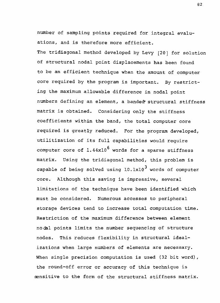
82

number of sampling points required for integral evalu

ations, and is therefore more efficient.

The tridiagonal method developed by Levy [2 0] for solution

of structural nodal point displacements has been found

to be an efficient technique when the amount of computer

core required by the program is important. By restrict

ing the maximum allowable difference in nodal point

numbers defining an element, abanded*

structural stiffness

matrix is obtained. Considering only the stiffness

coefficients within the band, the total computer core

required is greatly reduced. For the program developed,

utilitization of its full capabilities would require

gcomputer core of 1.44x10 words for a sparse stiffness

matrix. Using the tridiagonal method, this problem is

3capable of being solved using 10.1x10 words of computer

core. Although this saving is impressive, several

limitations of the technique have been identified which

must be considered. Numerous accesses to peripheral

storage devices tend to increase total computation time.

Restriction of the maximum difference between element

nodal points limits the number sequencing of structure

nodes. This reduces flexibility in structural ideal

izations when large numbers of elements are necessary.

When single precision computation is used (32 bit word) ,

the round-off error or accuracy of this technique is

sensitive to the form of the structural stiffness matrix.

83

However, no checks are provided for assessment of the

error introduced.

The method presented for calculating structural element

stress components by extrapolating stress matrices to

element boundaries has in certain instances been found

to result in stress components exhibiting finite dis

continuities between adjacent elements. These discontin

uities are inherent to the finite element displacement

method, and are a result of interelement force equili

brium not having been satisfied. Although these dis

continuities are frequently subjected to some sort of

averaging, the author has chosen to identify them for use

in the evaluation of the relative merit between differ

ent finite element idealizations.

The quadratic .element has been found to be quite suitable

for the analysis of thick pressure vessels. Both cylin

drical and spherical pressure vessels have been analysed.

By increasing the number of elements in the idealization,

the cylindrical pressure vessel model was able to pre

dict displacement and stress components which were within

.7% of theoretical values. The spherical pressure vessel

analysis resulted in a predicted maximum displacement

value within 3.87% of theory but discontinuites in

predicted stress values resulted in 60.% errors in

stress values at boundary surfaces. This indicated that

a more refined idealization was necessary using the

84

technique of extrapolating stress matrices to element

boundaries. It is suggested that alternate methods of

determining element stresses may prove more efficient.

The analysis of stresses in a circular disk due to a

centrifugal force loading condition has served to

demonstrate both the quadratic element's ability to repre

sent body force loading and the need for computer

program capabilities to internally generate nodal point

loads due to distributed surface and body forces.

Predicted stress values obtained were within . 1% of

theoretical values. User's specification of nodal point

loads was found to be possible only for regular shaped

elements (defeating the purpose of elements having curved

boundaries) , time consuming, and susceptible to input

errors.

Determination of axial stress concentrations in a cylind

rical rod in tension due to a spherical inclusion resulted

in accurate results being obtained witha minimum number

of elements. Initial idealization resulted in predicted

axial stress values in agreement with theoretical

values to within 1.06%. Also demonstrated was an in

ability to match boundary conditions in substructure

analysis of local patches of elements from the ideal

ization. In this substructure analysis it was found

that original boundary stresses were not reproduced on

the boundaries of refined models. It is felt that this

85

discrepancy is due to violation of displacement com

patibility between original and substructure models.

Resolution of this problem is suggested for future

study.

Investigation of the quadratic element's ability to

analyse flexural problems has shown that finite element

idealizations for plate bending must comply with all

restrictions imposed by plate theory if reasonable

results are to be expected. Also, the inadequacy of

single precision calculation using Levy's tridiagonal

solution technique for this type of problem has been

identified. When double precision calculations were

used, deflection and stress results were obtained within

.25% and 4% respectively of theory.

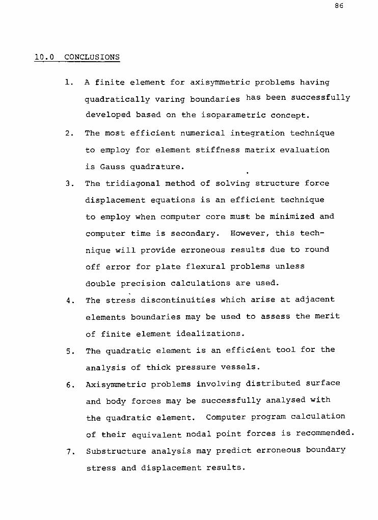
86

10.0 CONCLUSIONS

1. A finite element for axisymmetric problems having

quadratically varing boundaries nas been successfully

developed based on the isoparametric concept.

2. The most efficient numerical integration technique

to employ for element stiffness matrix evaluation

is Gauss quadrature.

3 . The tridiagonal method of solving structure force

displacement equations is an efficient technique

to employ when computer core must be minimized and

computer time is secondary. However, this tech

nique will provide erroneous results due to round

off error for plate flexural problems unless

double precision calculations are used.

4. The stress discontinuities which arise at adjacent

elements boundaries may be used to assess the merit

of finite element idealizations.

5. The quadratic element is an efficient tool for the

analysis of thick pressure vessels.

6. Axisymmetric problems involving distributed surface

and body forces may be successfully analysed with

the quadratic element. Computer program calculation

of their equivalent nodal point forces isrecommended,

7. Substructure analysis may predict erroneous boundary

stress and displacement results.

87

The quadratic element will predict reliable stress

and displacement results where bending deformation

predominates (e.g. thin plates) providing finite

element idealizations meet the assumptions of

plate theory and double precision calculations

are used.

88

11.0 RECOMMENDATIONS

1. Development of a routine within the program presented

to calculate nodal point loads due to distributed

surface and body forces.

2. Investigation of necessary conditions in sub

structure analysis to insure reproduction of

original boundary stresses.

3. Investigation of alternate methods for predicting

element stress components.

4. Investigation of alternate techniques for the

solution of the structural equilibrium equations

for one which is less sensitive to round off error

or modification of the existing program to a

double precision version for the Sigma 6 computer.

5. Extension of the program's options by including

thermal stress calculation and two dimensional plane

stress/strain analysis capabilities.

6. Provide in depth comparisons with other computer

programs and convergence studies to verify program

efficiency.

89

12 . 0 REFERENCES

1. Timoshenko, S. and Goodier, J., Theory of Elasticity(McGraw Hill Book Company, Inc., New York, 1970)

2. Timoshenko, S., Strength of Materials, Part II

(Van Nostrand Reinhold Company, New York, 1958),third edition.

3. Clough, R. and Rashid, Y. , "Finite Element Analysis of

Axisymmetric Solids", journal of Engineering Mechanics,Amer. Soc. Civil Engrs., 71-85, (Feb. 1965).

4. Wilson, E., "Structural Analysis of Axisymmetric Solids",AIAA Journal, Vol. 3, No. 12, 2269-2274, (Dec. 1965)

5. Crose, J., "Stress Analysis of Axisymmetric Solids

with Asymmetric Properties", AIAA Journal, Vol. 10,No. 7, 866-871, (July 1972).

6. Ergatoudis, J., Irons, B., Zienkiewicz, 0., "Curved

Isoparametric'Quadrilateral'

Elements for Finite

Element Analysis", Int. Journal Solids Structures,

Vol. 4, 31-42, (1968).

7. Irons, B., "Numerical Integration Applied to Finite

Element Methods", Conference on the Use of Digital

Computers in Structural Engineering, University of

Newcastle, England, July 1966, (revision from author

Nov. 1973) .

8. Ergatoudis, J., "Isoparametric Finite Elements in Two

and Three Dimensional Stress Analysis", PhD. Thesis,

University College of Swansea, Wales, (Oct. 1968).

9. Zienkiewicz, 0., Irons, B., "The Isoparametric Finite

Element System-A New Concept in Finite Element Analysis",

Conference on Recent Advances in Stress Analysis: New

Concepts and Techniques and Their Practical Application,

Royal Aeronautical Society, 35-40, (March 26-29, 1968).

10. Zienkiewicz, 0., Irons, B. , Ergatoudis, J., Ahmad, S.,

Scott, F., "Isoparametric and Associated Element Families

for Two and Three Dimensional Analysis", Finite Element

Methods in Stress Analysis, Ivar Holand and Kolbein Bell,

eds., Trondheim, Norway: Tapir Publishing, The Technical

University of Norway, 383-432, (1972).

90

11. Zienkiewicz, 0., Irons, B. , "Isoparametric Elements",Finite Element Techniques in Structural Mechanics ,H. Tottenham and C. Brebbia, eds., Southhampton

England Stress Analysis Publishers, Southhampton

University, 283-301, (1970).

12. Zienkiewicz, 0., The Finite Element Method in

Engineering Science, (Mc Graw Hill Book Company, Inc.,London, 1971) , second edition.

13. Irons, B., "Engineering Applications of Numerical

Integration in Stiffness Methods, AIAA Journal Vol.

4 No. 11, 2035-2037, (Nov. 1966).

14. Irons, B., "Economical Computer Techniques for

Numerically Integrated FiniteElements"

Inter.

Journal for Num. Meth. in Eng., Vol. 1, 201-203,(1969) .

15. Irons, B., "Quadrature Rules for Brick Based Finite

Elements", Inter. Journal for Num. Meth. in Eng.,

293-294, (1971).

16. Gupta, A., Mohraz, B. , "A Method of Computing Numeri

cally Integrated Stiffness Matrices", Inter. Journal

for Num. Meth. in Eng., Vol. 5, 83-89, (1972).

17 Desai, C, Abel, J., Introduction to the Finite Element

Method, i/an Nostrand Reinhold Company, New York,19 72) , first edition.

18. Archer, J., "Consistent Matrix Formulations for Struc

tural Analysis Using Finite Element Techniques",

AIAA Journal, Vol. 3, No. 10, 1911-1918, (Oct. 1965)

19. Tottenham, H., "Basic Principles", Finite Element

Techniques in Structural Mechanics, H. Trottenham and

C. Brebbia, eds., Southhampton England: Stress

Analysis Publishers, Southhampton Univeristy, 1-30,

(1970) .

20. Levy, S., "IS02D", Computer Workshop in Finite Element

Methods for Stress and Other Field Problems, Schenectady,

New York: Union College Graduate and Special Programs,

Union College, (Aug. 19 73) .

21. Dario, N., Bradley, W. , "A Comparison of First and

Second Order Axially Symmetric Finite Elements", Inter.

Journal for Num. Meth. In Eng., Vol. 5, 573-583, (1973).

91

22. Hildebrand, F., Introduction to Numerical Analysis,(McGraw Hill Book Company, Inc., New York, 19 74) ,second edition.

23. Spiegel, M. , Advanced Calculus, Schaum's Outline Series,(McGraw Hill Book Company, Inc., New York, 1963).

24. Oden, J., Finite Elements of Nonlinear Continua,(McGraw Hill Book Company, Inc., New York, 1972)first edition.

25. Loeber, J., Knolls Atomic Power Laboratory, Schenectady,N. Y., Private Communication.

26. McCalley, R. , General Electric Comp'any, Schenectady,N.Y., Private Communication.

27. Glasser, T., Knolls Atomic Power Laboratory, Schenectady,

N.Y., Private Communication.

28. Timoshenko, S., Woinowski-Krieger, Theory of Plates

and Shells (McGraw Hill Book Company, mc.7~New YorK,

1959) , second edition.

29. Cook, R. , "A Note on Certain Incompatable Elements",Inter. Journal for Num. Meth. in Eng., 146-147, (1973)

30. Griffin, D., "Use of the Computer for the Elastic Anal

ysis of Pressure Vessels", The Computer in Pressure

Vessel Analysis, Papers and Discussions from ASME

Computer Seminar, Dallas, Texas, September 26, 196 8.

31. Ergatoudis, J., "Quadrilateral Elements in Plane Analysis

and Introduction to Solid Analysis", MS Thesis, Univer

sity College of Swansea, Wales, (June, 1966).

32. Wilson, E., Parsons, B., "Trapezoidal Finite Elements -

Their Derivation and Use for Axisymmetric Rotating

Bodies", ASME Presentation at the Design Engineering

Technical Conference, Cincinnati, Ohio, September

9-12, 1973. Paper 73 - DET - 47.

33. Rieger, N., Rochester Institute of Technology, Roch

ester, N.Y. Private Communication.

34. Martin, H., Carey, G., Introduction to Finite Element

Analysis, (McGraw Hill Book Company, Inc., New York,

1973) ,first edition.

35. Halbleib, w. , Rochester Institute of Technology,

Rochester, N.Y. Private communication.

92

13.0 APPENDIX A

It is noted that the function to be integrated in

Eq. 13 was of a sufficiently complex form to necessi

tate the use of numerical quadrature.

Numerical quadrature is a numerical procedure for the

evaluation of definite integrals. Geometrically it

requires the numerical determination of the area or

volume under the integrand's curve [23], To use

this procedure, sampling points are chosen within the

region of interest and the integrand is evaluated at

them. Based on these integrand values and the number

of sampling points chosen, an approximate value of the

integral may then be obtained.

Numerical quadrature techniques may be divided into two

basic categories [22] , those whose sampling points are

equally spaced over the region of interest (Newton-Cotes) ,

ana tnose whose sampling point are chosen at optimal

locations and have weighting functions associated with

them (Gauss) .

Using the Newton-Cotes formulae requires n sampling

points for the exact integration of a function of

order n-l whereas the Gauss technique requires

n/2 sampling points.

Using the finite element method, structural ideal

ization usually involves introduction of large numbers

93

of elements for which stiffness matrices must be

found. Efficient computing techniques rely on a

minimizing of the number of mathematical operations

necessary. For this reason Gaussian quadrature,

which requires the fewest sampling points to integrate

a function of specific order, is most frequently

employed [7] . In Gaussian quadrature, the integral

of a function f (x) is replaced by the summation:

-.1 n

J f(x)dx = Hi f (a.)

-1 ^X

(14)

n is the number of sampling points

H. is the weight coefficient associated with

sampling point i

a. is the abscissa of sampling point i

The theory for determination of optimal sampling

points and weight coefficients may be found in

Hildebrand [2 2] . Specific values for n = 2 through

2 4 are presented in Table V.

The procedure for evaluating the element stiffness

matrix, [K] is as follows:

Eq . 13 may be rewritten as :

si1

[K] = J J f (P,Q) dPdQ (15)

-1 -1

where f (P,Q) is a matrix in P and Q equal to

2tt[B]T[D][B] [N] ^rQ\det [J]

94

Integration may be performed in a manner similar to

the standard technique of evaluating double inte

grals. Substituting Eq. 14 intoEq. 15 while holding

Q constant, one obtains:

1 n

[K] = $ EH f(a Q) dQ

-1 i=lL x

Applying Eq. 14 again but with respect to Q, the

expression for [K] becomes:

n n

S H H -P r a a "1 (16)[K] = L... >, H. H. f (a., a.)1 J

j =1 1 = 1 j l* i'

jJ

The number of sampling points in each direction used

in Eq. 16 should be such that the volume of each

element is exactly determined[12] . The minimum

number of sampling points which are required is

determined by the order of the determinant of the

Jacobian matrix [J] .

For the quadratic element developed, the minimum

value of n is 2 . However the element developed is

for n = 3 for convenience in element stress cal

culations (Section 4.8).

Considering the case of n = 3 , the element stiffness

matrix is determined by the summation of the function

f (P,Q) multiplied by its weight function at the

nine sampling points shown in Figure 20.

95

Figure 20

Sampling Point Locations

for Gaussian Quadrature

TABLE V

96

AHMXNSVS,\,M) WKIUir |-'\CTOU.S H>H <;Yl'S!MAN IVl'KWIATIOrt

,-*"

J V-r^t,)

Abscissas-r, (Zeros of Legendre Polynomials) Weight Factors- w;

i= 2 /.--8

0.57735 02691 39626

0.QOQ0O OOOOO 00000

0.77459 66692 41483

0.33998 10435 34856

0.86U3 63115 94053

0.00000 00003 00000

0.53846 93101 05633

0.90617 98459 .'8664

0.23861 91860 33197

0.66120 93864 66265

0.93246 95142 03152

0.00000 00000 00000

0.40584 51513 77397

0.74153 11855 99394

0.94910 79123 42759

I. ooooo ooooo ooooo

-=3

0.83588 83383 83889

0.55555 55555 55556

n r. 4

0.65214 51548 62546

, 0.34785 43451 37454

--5

n-7

0.56888 83883 88389

0.47862 86704 99366

0.23692 68850 56189

0.46791 39345 72691

0.36076 15730 48139

0.17132 44923 79170

0.41795 91836 73469

0.38183 00505 05119

0.27970 53914 89277

0.12948 49661 68870

0.13343 46424 95650

0.52553 24099 16329

0.79666 64774 13627

0.96028 98564 97536

0.00000 00000 00000

0.32425 34234 03309

0.61337 14327 00590

0.S3603 11073 26636

0.96816 02395 07626

0.14837 43389 316310.43339 53941 29247

0.67940 95632 99024

0.86506 33666 88985

0.97390 65285 17172

0.12523 34085 11469

0.36783 14989 98130

0.58731 79542 366170.76990 26741 943050.90411 72563 70475

0.98156 06342 46719

0.36263 37833 73362

0.31370 66458 77387

0.222:3 10344 S3374

0.10122 35362 90376

0.33023 93550 012600.31234 70770 40003

0.26mi 06964 029350.13064 81606 94857

0.08127 43883 61574

10

0.29552 42247 147530.25926 67193 09996

0.21908 63625 15932

0.14945 13491 50531

0.06667 13443 08683

n-12

0.24914 70453 134030.23349 25365 38355

0.20316 74267 230660.16007 83285 43346

0.10693 93259 95318

0.04717 53363 86512

"i --16

0.095O1 25098 37637 440185 0.18945 06104 55063 4962350.28160 35507 79258 913230 0.13260 34150 44923 5383670.45801 67776 57227 386342 0.16915 65193 95002 5331890.61787 62444 02643 748447 0.14959 59888 16576 7320810.75540 44083 55003 033895 0.12462 39712 55533 8720520.86563 12023 87831 743880 0.09515 35116 82492 7348100.94457 50230 73232 576078 0.06225 35239 38647 8928630.98940 09349 91649 932596 0.02715

20

0.15275

24594 11754 094852

0.07652 65211 33497

n

333755 338H 30725 850698

0.22778 53511 41645 078080 0.14917 29864 72603 746738

0.37370 60887 15419 560673 0.14209 51093 18382 051329

0.51086 70019 50827 098004 0.13168 86384 49176 626898

0.63605 36807 26515 025453 0.11819 45319 61518 417312

0.74633 19064 60150 792614 0.10193 01198 17240 435037

0.33911 69713 22218 823395 0.08327 67415 76704 748725

0.91223 44232 51325 905563 0.06267 20483 34109 063570

0.96397 19272 77913 791268 0.04060 14298 00386 941331

0.99312 85991 85094 924786 0.01761 40071 39152 118312

n-24

0.06405 58928 62605 626085

0.19111 88674 73616 309159

0.31504 26796 96163 374387

0.43379 35076 26045 138487

0.54542 14713 88839 535658

0.64809 36519 36975 569252

0.74012 41915 78554 364244

0.82000 19859 73902 921954

0.88641 55270 04401 034213

0.93827 45520 02732 753524

0.97472 35559 71309 493198

0.99518 72199 97021 360130

0.12793 81953 46752 156974

0.12583 74563 46828 296121

0.12167 04729 27803 391204

0.11550 56680 53725 6013530.10744 42701 15965 634783

0.09761 86521 04113 888270

0.08619 01615 31953 2759170.07334 64814 11080 305734

0.05929 85849 15436 780746

0.04427 74333 17419 306169

0.02853 13836 28933 663181

0.01234 12297 99987 199547

Compiled from P. Davis and P. Rabinowitz, Abscissas and weights for Gaussian quadratures of high

order, J. Research NBS 56, 35-37, 1956, RP2645; P. Davis and P. Rabinowitz, Additional abscissas

and weights fcr Gaussian quadratures of high order. Values for --"64, 80, and 06, J. Research N'BS 60,

613-614, 1058, RP2S7.5; and A. X. Lowan, X. Davids, and A. Levenson, Table of the zeros of Lhe Lexendre

polynomials of order 1-16 and the weight coellicients forGauss'

mechanical quadrature formula, Bull.

Amer. Math. Soc. 48, 739-743, 1942 (with permission).

97

14.0 APPENDIX B COMPUTER PROGRAM ISOAXI

Bl. General Analyst's Information

ISOAXI is a finite element computer program for

the static stress analysis of axisymmetric

structures having axisymmetric boundary condi.-:

tions. The element used is a quadratic axisy

mmetric quadrilateral capable of representing

geometric boundaries of quadratic variation.

The assumed element displacement function is

also quadratic. Element stress-strain relations

are for a homogeneous isotropic material. Up

to ten different materials may be specified per

problem. Options not included at present are

internal calculations of body forces and surface

forces, thermal stress capabilities, and pre and

post processors for mesh generation and computer

plotting.

B2 . Programmer's Information

Program development was accomplished using a

Xerox Sigma 6 computer. ISOAXI is written in

Fortran IV and makes use of three temporary

files (2,3,4) for data storage and retrieval

during execution. Data input is from a card

reader (F:105) and output is to a line printer

98

(F:10 8) . The program is overlayed as shown in

B3 . and required 10 . IK words of main computer core

for execution.

B3. COMPUTER PROGRAM STRUCTURE

99

THESOl THES02

XTHES03

MTINVB

MAIN

ZEROM

MATM

THES04 MATRIX SOLVE

MTINVC

MATMS

STRESS

PRINPL

MATTSYM MATTMS

100

B4. SUBROUTINE DESCRIPTIONS

The functions of the subroutines shown in B3 . are

as follows:

1. MAIN executive routine for calling subroutines

2 .

ZEROM*

3 .

MATM*

4. THESOl

5 . THES02

6 . THES03

7 .

MTINVB*

8 .

MTTSYM*

9 . THES04

10 .

MATRIX*

initializes a matrix to zero

multiplies two matrices

calculates the shape functions and their

partial derivatives at the nine sampl

ing points.

reads the majority of input data and

writes it out for checking.

calculates the element stiffness matrices

and stress matrices at the sampling

points of each element

finds the inverse of a matrix and also

the value of its determinant

multiplies two matrices, first transposed

times the other and insures resulting

matrix is symmetric

extrapolates the stress matrices at the

sampling points of each element to its

midside nodes.

reads nodal point prescribed displace

ments and external forces, assembles

the structural stiffness matrix and mod

ifies it to accomodate prescribed dis

placements .

101

11. SOLVE*solves the structural equilibrium

relations for displacement using a mod

ified Gauss elimination technique

12. MTINVC* inverts a matrix using the Gauss technique

with pivoting

13. MATMS*multiplies two matrices

14. MATTMS*multiplies the transpose of a matrix with

a second matrix

15. STRESS writes nodal point displacements, calcu

lates and writes element stresses .

16 .

PRINPL*calculates principal stresses and dir

ection cosines

*Subroutines obtained from Levy [20].

102

B5 INPUT DATA FORMAT

Data input to ISOAXI is in the form of punched

cards . Data required may be generalized as

consisting of seven sets, (A-G) with the number of

cards required in each set depending on the par

ticular problem being solved. The order in which

input data should appear, its format, and definition

is presented below.

DATA SET A PROBLEM PARAMETERS (FORMAT 7T4)

KPNT - number of nodal points in problem (max. 600)

KELM - number of elements in problem

NGEO - number of nodes having geometric constraints

NMAT - number of different materials in problem

(max. 10)

NFREE- degrees of freedom per node (always 2)

NFOR - number of nodes subjected to external force

NPART - number of partitions in problem (max. 45)

DATA SET B NODAL POINT LOCATIONS (FORMAT 2F16.8)

X(1,J) - radial distance from origin of nodal

point J

X(2,J) - axial distance from origin of nodal

point J

(This set contains KPNT cards in sequen

tial order from 1 through KPNT.)

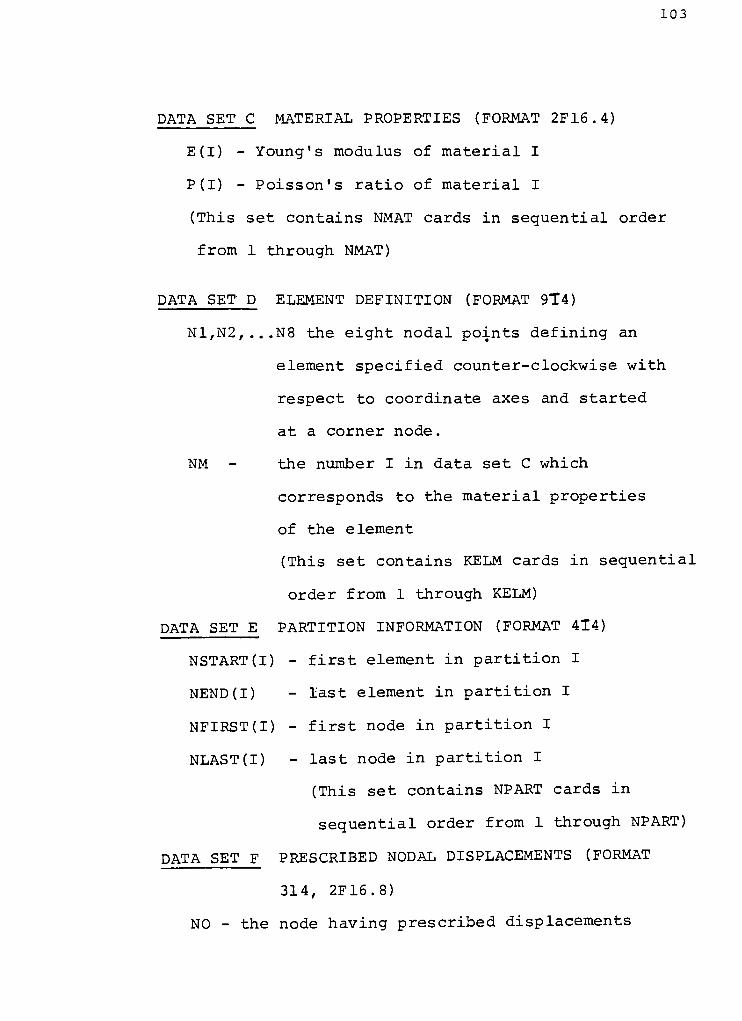
103

DATA SET C MATERIAL PROPERTIES (FORMAT 2F16.4)

E(I) - Young's modulus of material I

P(I) - Poisson 's ratio of material I

(This set contains NMAT cards in sequential order

from 1 through NMAT)

DATA SET D ELEMENT DEFINITION (FORMAT 9T4)

N1,N2,...N8 the eight nodal points defining an

element specified counter-clockwise with

respect to coordinate axes and started

at a corner node.

NM - the number I in data set C which

corresponds to the material properties

of the e lement

(This set contains KELM cards in sequential

order from 1 through KELM)

DATA SET E PARTITION INFORMATION (FORMAT 414)

NSTART(I) - first element in partition I

NEND(I)- last element in partition I

NFIRST(I) - first node in partition I

NLAST(I)- last node in partition I

(This set contains NPART cards in

sequential order from 1 through NPART)

DATA SET F PRESCRIBED NODAL DISPLACEMENTS (FORMAT

314, 2F16.8)

NO - the node having prescribed displacements

104

NA - 0 if radial displacement is specified, 1

if not

NB - 0 if axial displacement is specified, 1,

if not

U -

magnitude of specified radial displacement

V - magnitude of specified axial displacement

(This set contains NGEO cards)

#

DATA SET G EXTERNAL NODAL POINT FORCES (FORMAT

I4,2F16.4)

NODE - the node at which external force acts

FORR - the radial component of force acting at

the node*

FORZ - the axial component of force acting at

the node*

* the total force through 2tt radians

(This set contains NFOR cards)

105

B6 EXAMPLE OF COMPUTER INPUT-OUTPUT DATA

An example of computer program output is presented

in Fig. 2 4 and corresponds to the cylindrical

pressure vessel problem (1 element solution)

presented in section 8.1, Fig. 7. A sample list

ing of input data is not presented since computer

output includes this information.

First output by the program is all input data

information. This is done to facilitate data

checking and also provide model documentation

Printout of this information is in the same order

as presented in section B5 and is noted in

Fig. 24. Following this information, displacement

components of all structural nodal points are

output. Displacement output in Fig. 24 for

nodal point 1 indicates that radial and axial

displacement components are:

u = -.43032356 x 10~2in.

v =.37970068 x 10~3in.

Following displacement output, element stress infor

mation is printed. Four sets of stress information

are provided for each element's midside nodes. Each

set contains the following information:

EL - Element number

NODES - The 8 nodes defining element EL

106

STRPT - Midside node to which stress components

correspond.

SIGR - Normal component of stress in the

radial direction

SIGTHETA - Normal component of stress in the theta

direction

SIGZ - Normal stress component in the axial

direction

TAURZ - Shear stress in the rz plane

PS - Principal stress value

L - Direction cosine between PS and r axis

M - Direction cosine between PS and z axis

N - Direction cosine between Ps and the 6

axis

An example of interpretation of this information for

element 1, defined by nodes 12358764, the

stress components acting at node 4 (STRP 4) are:

a =-12188.5 psi

aQ= -21995.3 psi

a = -15.5 psi

z*

x =-3.2 psi

rz^

These stress components correspond to principal

stresses of:

15.5 psi in the -z direction (L=0. ,M=-1. ,N=0 . )

107

12188.4 psi in the -rdirection (L=-l. ,M=0 . ,N=0 . )

21995.3 psi in the +e direction (L=0 . ,M=0 . ,N=1)

FIGURE 2 4

COMPUTER OUTPUT - ISOAXI

3 m-j ( L'- N f Tu rr TO

ttil ^'U "*0 EF" ~

rLc"iirf'!^c.

>. .

J fM 0 C r. ~

-

-.r''

TrOTpI- P 1, r T ; I '

^T r

Ml)'^ rc

c"

")Ict-;-\'t < i Tr 07 i (_c , t

^jii"-:? of\c-f~

:u-Jr^"rrni To r^

\-jMOCc ^C DiO-yrT.ONjr

* <

108

v icJu r -0= r)T NAT- r ^_ ^ o T ki *

At^UL

1

EL E*Ent

1

2

5

k

5 . :1 :

S.<T

7.5.

7.3

7 r<

,1 rl

3

o i < ] :'

1 j

7 1-1.0 .'-13

mohulus or elas tt":tty -nxssivs =a-

3 is r:am p. 35^

*ATE- I AL

~3 <T1

112 5 5 3

1 1

5 11 .flfj^nfif:^

7 l ^ . d^nr*?!^

1 37127. 39^5

? 143495.552-5

3 37123. 83?5

5-157*379.625^

7-S23 31 <?.=! SB

a

* * *0 !<: =>L ACE"ENT* * * *

7 5 4 1

1

.my

NO r;F e? AD IAL(> 4XIAL17)

1 -.4333?35SE-ri2

2 -.43?7315?E~^?

3 -.4344545 3E--J2

4 -.4533541 3F-^2

5 -.45213232E-f*2

5 -.52541C35E-t=,2

7 -.5248457?=;-^2

p -

.52583 3~8E-~?

EL 1 N"3ES 1 ?

, 3 79 7^35 8="-:, 3

. 1C1S737F-T 3

, *3r m 5*3 ij E T 7:

,?S1 79281E-] 3

, 3f,575455F t-

,1S3<i715E-i 3

=)," nfl r-T'h'F "j "!

, 1^5 55 87""r-! 3

3 5 3 7

ctGp -95 94,-i<;lG"rMF'rA -2^375. 7ST1Z

Pc -.2L

-. Till"7

-> > v>

109

Figure 2 4 (Continued)

s<r-omii,:'-

-- ? Q 9

?~

f=,v' -

.

""

12 - 4 "' VJ .Ji 7 "I'

3<r -?337=.7L.,-.

r-

. ri-,.'L.!;^^

t.:~ri:

EL 1 \1 ^r r 1 H I 5 ^ TS

'i-rra^

;T^o -121= 3. ^-lG"ruE"ri -'-"'Its,

7TT""'

-i \.^ i)',-~r

-'

c -H.rL -'"

~'"13?-1 .

'^v

oc-

-1^19'. ?L -.900037-1 .

,i:>2a37N ..i -.-2 T^-

c -?^14S.7L .

*

7f. 'f ? * .fl

"*-

"Mh"vj 1 "rj.^i~

EL 1 N0 9ES 1 2 3 5 3 7 5 .ArToo-r

*

Si 3d -15223. 5-lGTHETA - ^ 54 3. f 5"G Z 7.7TAUC"'

_?

Pr 7.3L .f!-:-:-.19*-l .'l^'ilON.C'-nh*}-

Pr -15223. 5L -9999^8*-..3 135H4M

?r -2^8 4 5.sl .^-ir.in* ny in o m i .s^e^^

EL 1 NODES 1 2 3 5 3 7 5*^'OT

a

STG=> -12138 .ESIG^HETA- ?1 99 5. 5 ST^? -^

Pr -15. SL -.afl!)?55'-l..??M0N .3 -Xl 'TS ^

Pr -12138. ^L -.999999* -.1?U2J9N .1 "0 'Tj

pc -219 95. 5L .3?n^Pi .fJOHSrlCN l..lr:f5->Tn

*c tdP* 3

110

c-

c

c

c*

FINITE ELEMENT PROGRAM ISOAxI

FOR AXISYMMETRIC STATIC STRESS

USING AN 8 NODFO QUADRATIC

ELEMENT SUBJECTED TO AxISYMM^TRlC

AnD GEOrETRIC CONSTRAINTS

ANALYSIS

ISOPARAMETRIC

LOADING

* *

MASTER OF SCIENCE THESIS

F.X.J6NLCIK JUNE'1974

SCCHESTE^ INSTITUTE OF TECHNOLOGY

n n if. n n r"

if. *. is

* *pARAr--c.TfPS:

* * * *

KPnT-max IMUM

NGEO-MAXlMUM

NM A T -MAXIMUM

NFREE-NUrBER

\FOR-MAXl -luM

NP&RT-MAXl'-UM

number cf nqdes=600

number of geometric constr a i nts=-600

number of different material propert i es1 0

of degrees of freeqom per node(always 2)

number of External nodal forcls=Sqo

number of partiti0ns=45

C* * ^VARIABLES!

J-".*******

X(l#

X( 2>

E( I )

PII)

\STA

nEnD

nFIR

nLaSs

NF( I

NS( INat iBVI IBV ( IU( 1

-

Ul 2#

STRP

PS-P

L*fl/

3IGR

J)-RAD

J ) -axI- Y 0 U \ G

-PCISS

RTl I )-

( I )-LA

STI I )-

T( I ) -L

) *NCO

j\)-0

*2)-C

/ 1 ) - r. a

, 2 ) -rA

KJ-RaD

K ) - A X ITNCDc

RINCIP

N-DlF..=-

jSIGTH

ial dista

al distan

s modulus

ONS RATIO

FIRST ELE

ST ELE.MEN

FIRST NOD

AST NODE

L POINT N

IF CONSTR

IF CONSTR

GNITUDE 0

GNITUDE 0

IAL FORCE

AL FORCE

A-T WHICH

AL STRESS

CTION COS

ETA-SIGZ*

AND S

NCE FROM ORIGIN OF NODE J

CE FROM ORIGIN OF NODE J

OF MATERIAL IOF MATERIAL I

MENT In PARTITION IT IN PARTITION I

E In PARTITION IIN PARTITION I

UMBER OF CONSTRAINT

aIn-D/ 1 IF NOT (RADIAL DIRECTION)

AINEOi 1 IF NOT (AXIaL DIRECTION)

F RADIAL CONSTRAINT

F AXIAL CONSTRAINT

THRU 2 PI RADIANS AT NODE K

THRU 2 PI RADIANS AT NODE <

STRESS COMPONENTS ARE CALCULATED

INESTAURZHEAR

-radial>hoop> axial*

STRESSES RESPECTIVELY

* * * * * *

;* * ^subroutines:

THES01^ THES02M THES03r

MATMn

ZEROm

c MTTSYMr

MATMS

w M A T T M Sr

M T I N V 3/*

THES04

c MATRIX

w SOLVEi

MT

INVCr>

STRESS

PRINPL

c# * * * * *

C* * *MAlN E

* * * * * j************

EXECUTIVE PROGRAM!

COMMON NPART/KPNT>KELM-NGEOiNMATjNFREE>NFOR

liNSTARTU5J ,NEND( 45>>NFlRST(*5)>NLASTU5!

CALL THES01

R fc W I N D 2

REWIND 3

REWIND 4

CALL THES02

REwlND 2

111

31

32

S3

3 4

45

Hi

8 3

a?

9 091

92

93

REWIND 4

CALL THES04

REWIND 37 E w I N D *?

CALL MATRIX

RE'WlND 3

REWIND '-

CALL SOLVE

REwlNJ 2R E w I N D 3

CALL STRESS

STOP

END

1

2.

3i

56

7 i

a

510.

MATRIX MULTIPLICATION ( DB > ( LXN I -D < LX* ) 3 I MXN )

SUBROUTINE MATMl DjB*D3#L> Mjn)

DIMENSION D(L*M>,3<M,N)>DB(L'N)

DO 110 J=1*N

DO HO 1*1 -L

u3( I> J )=0'

DO 110 K = 1 * M

110 D3( I -

J)0F3l I* J)+D( I<K)*B(K- J)

RETURN

END

2-

3.

4

5.

6

7.

8.

10

SUBROUTINE ZEROM

SUBROUTINE ZER0M(A*I><)

DIMENSION All)

II-U<

DO 10 J = l- IIAl J)=0.0

RETURN

E lO

112

C****SU3R0UTINE ThESOI

SU3R0UTINE ThESOI

c This subroutine calculates the shape functions and- TmEIR DERIVATIVES AT THE NINE QAUSS POINTS

- FUNCTIONS STOKED IN CF'JN I I , U I * I =G P '* U = SH APE FUNCTION

C RARTIALS STOfltO IN aup< k*l -m i *k=with respect TO KAl(l)- *-vITH RESPECT TO ET A ( 2 ) > L = s* aRE FunCT I ON* M =GA'JSS PT*

COMMONNPART-

<PNT-<ELMiNGEO-NMAT>N TREE* "J FOR

l/\,3TART(*5),NEND(451*NFlRST(*t3)'NLA:;T(t5)

DI -1 E.n SIGN E<K9)*ETA(9),AUP(2*8*9l*CFUN(9/8)

C < * * * PARTIAL. DERIVATIVES OF aHARE FUNCTIONS w I T w RESPECT T 0 P

rUC0l(X*Y)=25*

FUC02(X-Y)a-X'il("UC03( X, Y >= 25*

FUC04(X*Y)=5*rJC05(X/Y)=25*F U C 0 f, I X * Y ) = - X * (

CUC07 I X-

Y > = 25*

FUCOS I X* Y ) =>i5<M

>*** PARTIAL DERIVaT

trUC09IX*Y)=.25^

rUClO( X* Y>.5*<

FUC11 ( X, Y>=23*

FUC12(X*Y)=-Y-(

FUC13( X* Y=^25*

rUClt ( X-Y >=-.5*

FUC15IX* Y ) = i25*

FUC16I X* Y)=-Y*l

:**** SHAPE FUNCTIONS

(l' +YUlX^Y-i' ) + (l+X)^(l+Y) )?Y )

(m(1.+v)*(-X +Y-1. ) l-ll.-Xl^lli+Y) )1 , y**p )(\. ( 1 . -Y )m I -x-Y-1 . ) )I1-X)*(1-Y) ). aY )

ll.-Y)MX-Y-l) + (l.+X>*(l-Y))"Y*^ )

VES OF SHAPE FUNCTIONS WITH RESPECT TO 0

ll+X)MX +Y-l.) + (l.+X)*(l'+Y) )X^*2 )

(l.-XIM-X +Y-l. I + Il.-X)*(l.+Y) ).-X )

[-(1-X)*(-X"V-1 I )-(l"-X)*(li-Y) |

(-(l.+X>*(X"Y-l-))-(l'+X)*(l.-Y))

.+X )

' FNl(X*Y):-~.25*(l.i-X))Ml'fY)(l.-X-Y>

FN2IX*Y) = 5*(1'-MX**2) )*( 1 .+Y )

FN3(X>Y)a25^(lX)'Ml--fY)'>(-X +Y-l.)FN<r(.<-Y)a5*(lt-X)'Ml(Y**2))

FN5(XjY)25*(lX)'Ml.-YU(-X-*-li)FN6I X - Y ) = '5-M.l . -X**2) *( 1 . -Y )

FN7(X*Y) = '25JMli+X)JMl."'YU(X-Y-l)

rN8lX*Y)=-5*(l.+X)*(l-Y**2)r-

C**** DEFINE GaUSS POINTS ( E< I ( I ) , ET A I I ) ) * I! * 9

X1=0. 77459667

X2 =0. OOOOOOOO

EKIEKI

EKI

EKIEKI

EKI

EKIEKI

EKI

ETAET\

ETA

ETA

ETA

ETA

ETa

ETa

ETa

1 ) - X 1

2 ) "-Xl

3)"-Xl

4)X2

5)X26)=X2

7 )=X1

8 ) = X 1

9 ) X 1

1 ) " - X 1

2)=X23)=Xl

4 ) =-Xl

5 )oX2

6)=X1

7 )-Xl

8 )-X2

9)=X1

DO 50 1=1*2DO 50 U=-l*8

DO 60 K=l*9

aJP( I*U*K>=0. OOOOOOOO

S2

44'

|;

S9

90

9;

92

939*

35'

'Jh

9?

*a

9'j<

CO'

010?'

03

04

05

06

07

oa09,

10 -

ii'

13

114

115'

116

.17

.13

I^L^1

2223'

24.

2526'

27.

23>

29.

W * *

C-i*

19

60 CON50 CON* EVAL

DO

^AR

AUPA JPA UP

AUP

AUP

AUP

AUP

aUR

? *=>

AUP

AJP

*UP

AUP

AUP

AUP

AUP

AUP

CON

AUP

113

TlTlUa

19

Tl(

NU

NUTE99

1 >> >!

99

i

2-j

J>L.

2

2

212

( 2

Tl(2

OF

WITH PE

PARTIAL DERIVATIVES AND SHAPE FUNCTIONS AT 9 SAMPLING POIN

K = 1 * 9

OF N'S

= AUP= AUP= AJPaAJ3

= AU3

= AUp

a A J ?= aUP

N' S

A J P

=AjP

= aUP

= AUP= AUP= AUP

=AUP

= AUP

A. *

1*

1*\,1/

1*

1 /

1 *

WITH

t

2*

2,I

I 2it

! +

) *

) +

) +

) +

I +

) +

RE

) +

NUE*3*9) IS FORMED

SPECT

FUCO

FUCOFUCOFUCOFuCO

FuCOFuCOFUCO

SPECT

PUCO

*jy

FUCl

FUCiFUClFuCl

FUCl

TO P

1 (EKK2< EKl I3< EKI I4( EKI (

51 EKI (

61 EKl (7IEKI (

8 ( E < I (

TO a

9 ( E < I I

0 I 7 ''. I (

1 1 < I (

21 E<I (

3IEKI I4(EKI (5IEKI I6IEKI (

ETA

ETA

ETA

ETAETA

ETA

ZT.\

ETA

ETA

C I A

ETa

ETa

ETa

ETA

K) )K) )

K) )

K) )

< ) )

Kl )K) )

K ) )

) )

I )) )

) )

I )

C**** SHAPE FUNCTIONS AT NINE SAMPLING POINTS

2002

2001

2000

! > v 's v-

D

D

C

c

J

c

Cr

C

cr

r

W

E

ti

w

11

RET i

END

0 20 2FUN

OnT

ONT

0 2FUN

FUN

rUNFun

FUN

F'UN

"UN

fun

OnTRIT

nD

EWIRIT

(CF

00

00

1 1

IN

IN

00

I I

( I( I

1 1 =

2 U =

* J I =>

UEUE

0 1 =

) =

1*9

1*3

0*00000000

( I

1 1

( I1 1

1 1T Ll

L 1

E

FI

ND

ElUNRN

2) =

3) =

4 ) =

56

7

3

UE

AUP

LE 2

2

2) I I

( I -rl

) =

) =

1 =

1*9

FN1

FN2FN3FN4

FN5FN 6

Fn7

FN8

(EKI

(EKI

(EKI

I EKI

(E<I

(EKI

(EKI

(EKI )

ETAI I

ETA< IETAI IETA( I

ETA(ETAIETAI

ETAI

AND CFUN TO TEMPORARY FILE 2

( AUPI J*K*L) *U1*2) *K<

) * 1=1*9) *M= 1 j8l

1*8)*L=1*9>*

12<

3.

t

5

67.

y

13 *

11 '

12.

13.

17.

12 >

19.

20.

21.

2223-

24.

25

26.

27.

28.

29.

30.

31

32.

33-

3<,

35 >

36.

37.

33.

35.

40.

4l .

42-

43-

-

4 i

45.

46.

47.

43.

49.

50.

51 .

52.

S3.

54.

5b

56.

57.

53.

59.

60.

61.

62.

63.

64.

65.

6 6 <

67.

63 .

69.

70.

71.

72.73.

74.

7-J.

76.

77.

72.

79.

SO.

114

C>*** SUBROUTINE TmES02

cSUBROUTINE THES02

COMMON NPART-

<PNT*<ELM,NQEO*NMaT-NFREE* NFOR

lNSiART(45)/NEND(45)*NFlRST(45)*NLAST(45)

DIMENSION NODI 8 > *EMOD( lO)*P(10)*XE(8*2)

1'APU(2,(S-9)*kFUN<9*8>*x(600-2)

R E w I N D 2

?'**' ^Ea SHAPE FUNCTIONS RFUn AND THEIR PARTIAL DERIVATIVES FR01 FILE

R E A D ( 2 ) ( ( (APU(U*K*L)*Uil/2)iKi*8)*La!l*9)*1 1 i rfuni : ,mi , 1 = 1,9 ) , *<=: a j^ E I m D c:

re h Ind *

Z *>>* READ DaTa SET A

READ! 105/10 )KPNT,KEL"!*NGEO*NHAT' NF REE* NF OR* NPART

wRITEjlOS*20)<PNT*KELM,NGEO^NMAT,NFREE*NFOR*NPARTWKITt(lG8*4l)

Z !.*** READ DaTa SET BDO 30 I=l*KPNTREAD I 105 j 40) ( X( I* J) * Jl*2)

n"RIJEI 108*50 ) I* I X( I* J) - J-l j 2

30 CCN-INUEr

wRITEl 108*79)r*

C->** READ DATA SET CDO 60 U = 1 * N M A T

REaDI 105>70)EM0D( J)*P( j J

WITE( 10a*80 >u*EmODI J) ,P( J)60 CONTINUE

REWIND 3

WRITEl 108*105)

:>*** READ DATA SET DDO 90 NX=1*<ELM

READ! 1 05-100 ) (NOOI J) * Jl*8 ) , NEP

wRITE(i0fc*H0)N-X,(N0D(U)*Jl*8)*NEPDO 120 1=1*8JJNOD( I )DO 120 IX'=1*NFREE

120 XEl I> ixieXi UJ* IX)

*?* COMPUTE ELEMENT STIFFNESS MATRIX

CALL THEs03(APJ*RFUN*Nx*EM0D(NEP)*P(NEP) *XE*NOD)90 CONTINUE

10 ^ORMATI 714)

20 F0RMaT(1X*39HT0TaL NUMBER OF NODAL POINTS'.... *I4/

11X*39HT0TAL NUMBER OF ELEMENTS. ........14/21X* 39HNUMBER CF GEOMETRIC CONSTRA I NTS . . . * I 4/31X*39HNUM6ER OF DIFFERENT MA TER I ALS * *I4/

41X*39HDECREES OF FREEDOM PER NODE *.*I4/

51X*39HNUMBER OF NODES SUBJECTED TO FORCE.* 1 4/61X*39HNUMBER OF PARTITIONS *IV/)

C40 FORMAT ( 2Fl68 )

41 FORMATI 1CX*4MN0DE* 10X*i3hR CO-ORD I NA TE* 10X * 1 3HZ CO-ORDINATE/)50 FGRIiAT(!0X-M-7X,F16.4-7X-Fl6.4l

70 FORMATI 2F16 .4 )

79 FORMAT( lx*8HMATERlAL*2x*2lHM0DULUS OF ELAST IC I TY , 2X* 14HP0 ISSONS RIT 10/ )

80 FORMATI 1X*4X* 14* 7X*F16.4>2X*F14. 4)

100 FORMATI 914)

109 FORMATI 1X*7HELEMENT*9X,14HELEMENT NODES* 9x * 8HMATER I AL/ I110 FORMATI 1X*3X* 14, 814, 2X, 12 )

C

Z >>*>!* READ DAT A SET EC

DO 2000 Jal*NPARTREAD! 105*2001 ) NST ART ( j ) , NEND (J ) *

NP"

I RST I J ) * NLAST ( J )P001 F0RMATI4I4)

115

81

82.

S3.

it u .

;,6

WRITEI108*2002)NSTART(U>*NEN0(J>*NFIRST(J)*NLAST(J)

2002 FORMATI 10X,4( I4*10X ) )

CONTINUE

RETURNEnd

116

12.

3.

4

56

7.

2

310.

11

12.

13.

1 *

15

16.

17.

IS.

19.

20.

2122.

23.

24.

25

26-

27.

2?.

29.

30.

31 .

32-

33.

3" .

35.

36.

37.

38

39.

-.0.

41 -

42.

-.3.

-4 ,

45.

*6.

48.

-9.

50.

51

52.

53.

54.

C**** SUBROUTINE THES03 SEPTEMBER 18,1973 F X. UANUClKSUBROUTINE THES03I APJ,RFUN,NK0,E,P1,X*N0DE)

COMMON NOART,K,">NT* KELM, N3E0,^MAT,NFREE* NFOR

1'NSTarTI45),NEND(45)*nfIRST(45)*NLaST(45)

DIMENSION RFUN(9,3)*APul28*9),CE(16*16>*3(4,l6)*SCR(2*8)*N0DE|8

l*X(a,2)*O0(2j2l*C(9),D(4#4)*AlNT(4*16*9>*ClNll6,l6)1 - R R < 1 i 1 ) i C F U N ( 1 , S )

L A H M *

; * * ii ',

-****

1 -RR< 1,1 ) ,CF UNI 1*3 )

DEFINE GAJ3S QUADRATURE wElQrlT COEFFICIENTS

^10. 5555 5 536w 2-0. 83332:- 39

C I 1 ) = w > * 2

C t 2 ) = w 1 * W ?

CI3lwi*.2C(<+)=W1*W2Cl 5 >=W2**2C ( 6 ) = w l w 2C I 7 ) = w 1 * >: 2C I 8 ) =Wl*W2

C I 9 ) = W 1 * * 2

INITIALIZE ELEMENT STIFFNESS MATrIx CE TO ZERO

CALL ZEROMI CE* 16,16)

CALCULATE ELASTICITY MATRIX D

;?*** SET ELEMENT ELASTICITY MATRIX TO ZERO

CALL ZER3-1(Di4*4)ECl=Pi/( 1 .-Pi )

EC2=( 1 . *2*1 )/( 2*< 1 .-PI ) )EC3 = E-> ( 1 ."Pi ) /( I 1 +P1 ) ?< l .-2 *P1 ) )

EC*=EC1*C3

D( 1*1 )=EC3

Dl 1*2)=EC4

D( 1*3)=EC4

D<21 )=D(1*2)

D(2*2)-C3

0(2*3) nC4

Dl 3*1 )D( 1 -3)Dl 3*2)=D( 2*3)Dl 3*3)=EC3

; * * * -

0(4*4 )=EC2*EC3

CALCULATE ELEMENT STIFFNESS MATRIX

C**** C

cD

c

30 CC * * i- < c

cC***v C

CC

j-

* * v. cV

c

C * '. * * Ic

c * * * * c

DK

U

E

Ss

flfl

0 10

ALCUALL

0 30FUN I

ONTIaLCU

ALL

ALCU

ALL

ALCU0L = 6

ALL

NIT IALL

ALCU

0 20= 2*1= 2*1I 1*U

I2*UI 3*K

I 4* UI 4 , K

0 NG

LATEMAT-

Jl

1* J)

NUE

LATE

maTm

lateMTlN

LATE

2 83

maTM

ALIZ

ZERO

LaTE

0 1 =

P=l*9UACOBIAN

lAPU(l*l*NGP),X,AJ0*2*8,2)* ?

=RFUN(NGP* J)

PAD(CFU

JAC

VBI A

VOL

18 5*

I AUG

E ThM(3*

THE1*8

IAL DISTANCE TON* X* RR* 1*8*1)

OBIAN INVERSE AND THE

U0*2* AREA )UME ASSOCIATED WITH SAMPLING

C ( NGP )*RR( 1,1) *AREA

# APJI 1*1*NGP> , SCR, 2, 2, 8)

E B MATRIX TO ZtRO4,16)

.

B MATRIX AT SAMPLING POINT NGP

GAUSS SAMPLING

VALUE OF

POINT

POINT

ITS DETERMINANT

NGP

-1

)=SCR( 1* I )

)-RFUN(NGP* I 1/RRI 1*1 )

)=SCR(2* I )

)=SCR(2* I )

) = scr 1 1 , : )

200

;- 1> k- *

-7

K'* >,l

r. a-

V-

40G c:

.i> '' :

n '.' * *

117

CONTINUEINITIALIZE MATRIX CIN TO ZEROC*LL ZEROm( CIN*16*16)

CALCULATE STIFFNESS CONTRIBUTION OF SAMPLING POInT NGP MATRIX CIN

MULTIPLY MATRIX 3 TImEs D TO GET STRESS MATRIX AINT AT PQlNT NQP

CALL MaTm(D*3*AInTI1,1,NGd)*'*'4*16)"ULTIsi y -aTrI* aInT TImES TmE 3 MATRIX TRANSPOSED TO GET CIN AT POINT NGP

CALL ""TTSYM(5,AI\T(l*l,NGP)iClN*16,4*16)

DO 'OC U = l,16DO 400 < = 1 , 1 6

CE(U,<)=cE(U,K)+VOL*ClN(U*K)INUE

CONTINUE

wRI'E THE ELEMENT STIFFNESS MATRIX* NODES* AND NUMBER TO TEMPORARY FILE 3

w^ITE(3)|(CE(U*I)*J!5l*16)*Ial,l6),(N0DE(I),Inl,8),N<0

WRITE THE STRESS MATRICES AT ThE NINE SAMPLING POINTS OF EACH ELEMENT TO 4

WRITE! 4. ) ( I (AlNT( I , J*< ) i I =1,4)*J31,16)*K = 1*9)1* I NCDEIL )*L = 1,P )

KETURN

SUBROUTINE MTTSYM(D*3*DB*L*M'N)

DIMENSION DlM*L) *B(M*N)*D3(L'N)

DO 110 J*1*N

DO 11C 1=1* LIf I I.LT. J) DB( I* J)=DB(U* I >

IF(I.LT.U) CO TO 110

Db( I, J)=0*OC0C0C00CDO 120 K=1*M

120 D3(I,J)=D8(I*U)+D(K*I)#B(K,J)

110 CONTINUERETURN

END

118

MATRIX INVERSION WITH yALU^ OF DETERMINANT 6/9/71

SUBROUTINE MTINV3 I A* N* DETERM >

13 MATRIX BEING INVENTEDIS MATRIX SIZE

10

15

20

30

if. if.

40

43

50

60

70

80

5

90

95

100

105110

*

130

140

150

160

170

200

26'J

270

31 0

320If. If

330

340350

wif. i/.

380

330

400

420

430

450

451

550

C *

C

C600

falO

620

630

640

650

660

670

7uO

705710

740

IS MATRIX SIZE, ,

DIMENSION IP1V0T(9)*A(N*N)*INDEX(9,2)*PIV0T(9)

-. if, if, if. if. >c >S * * * * * * * * *

INITIALIZATION* * * * * *

*

* *

* * *

* *

*

DETERM1.0

DO 20 J=l/N

IPI VQT( J)=0DO 5 5 0 I -> 1 * N< if. >s if. f- 'l V *

SEARCH ="0R PIVOT ELEMENT

'l',< H " H H If. If,

^;x = : . o

DO 105 J=1*NIF ( IPIVQTI J) -1 160,105,60DO 100 K=1,NIF ( IPIVOTI <)-l 180*100, 740IF (A3S(AMAX)-A5S(A(J*K) ) (85*100,100I R 0 w = uICOLUM=KAMAX=A(J,K)

CONTINUE

CONTINUEI3IVOT( ICOLUM )IPIV0T I ICOLUM +l

f- If, >f. If, ft iH y. ^ ,|(, ^ ^ ^ ^ , * ^ ^ ^ ^ ^ ^ +

interchange rows to put pivot element on diagonal******?*?**

IF ( IROW-ICOLUM 1140*260*140DETERm=-DETERMDO 200 L=1*N

3WA3=AI IR0W,L)A( IROW,L l-A| ICOLUM, L)A( ICOLJM,L)=SWAP

INDEX'

I * 1 ) a IRQ W

INDEX( I*2>=IC0LUM

********

*

* I1

* *

.7. i\ if. if, if, if. jp, if. if. if.

A( ICOLUM* IC0LUM)=1 .0

DO 350 L=1NA I ICOLUM* L)-A( ICOLUM* L)/P I VOT( I

.-. n if it. if. 1: n f. j * H if,

REDUCE NON-PIVOT ROWS". if. 1;. if. if. >f. if. if, if, >s

DO 550 Ll=l*NIr"(Ll"ICOLUM)400,550,400

T=>A(Ll* ICOlUM)IF<T.EQ0-0) GO TO 451

AlLl, ICOLUM)=0.0

DO 450 L=1*NA(L1*L)=A(L1*L)"A(IC0LUM,L)*T

CONTINUE

CONTINUE

CONTINUEV- *

INTERCHANGE COLUMNS

^^^i^jji^*

DO 710 I1*NL=N+l -IIF <INDEX(L*1)INDEX(L, 2) (6 30,7*0*630

JROwINDEX(L#l )JC0LUMlNDEX(L*2)

DO 705 K = 1 * N

SWAP=A ( K, JROW )A ( << JROW ) =A ( K, JCOLUM )Al <i JCOLUM 1 =SWAP

CONTINUE

CONTINUE

RETURN

END

*

**

119

.if. *

C

Z x. if. If.*

C >

Q if. if, if, if,

2r-

v.

3C*

Z f,

C

SU3R0UTINE THES04

EXTRAPOLATES STRESS MATRICES AT SAMPLING POINTS TO ELEMENT MIDSIDE NOD

CQhmCN NPART*<PNT*kELm,ngEO*NmaT,nfrEE*NFOR

.*nSTaRT(45),nE.ND(45)*NFIR3T(45)*NLAST(45)

DIMENSION STR|4,16*4)*nA(4),N0DE(8),DB(4,16*9)

REwlND 4

DEFINE WEIGHT COEFFICIENTSAA= 1.^7833056Ac = -0 . 66666657C = 0 . 1 s 7 & 3 6 1 1

:C 1 J0G = 1*KELV|

READ ELEMENT STrESS MaTrIcES AT GAUSS SAMPLING POINTSand also Element nodal point numbersPEaDI 4 ) ( ( (DBI I*J*K)*I=l*4)*J = l,l6)*K*l*9>,* (N00EIL) *L=1*8)

initialize midside node stress matrices to zeroDO 2 11=1*16DO 2 Jl=l*4

DO 2 <i=i * 4

STR (Jl, 1 1*K1)0. OOOOOOOO

CALCULATE STRESS MATRICES AT MlDsIDE NODES

DO 3 12=1*4

DO 3 U2=l*16

STR(I2,U2*l)=AC*DB(I2*u2,4)+ABD3( I 2* J2* 5 ) *AA*DB ( 12* J2*6)STR(I2,U2*2)=AAD3II2,u2,2)+AB*03( I 2, U2* 5 ) + AC*DB ( 12, J2,8STR(I2,U2'3)=AADB(I2*U2*4)+AB03( I 2* J2* 5 1 +ACQB ( 12* J2*6STR( 12, J2*4)=ACDB( I2*U2*2)+AB0B( I 2* J2* 5 1 + A A*D8 ( 12, J2*8

CONTINUEDEFINE MIDSIDE NODES ASSOCIATED WITH CALCULATED STRESS MATRICESDO 4 U6=l*4

U 7 = 2 J 6

7.a(U6)=nODE( J7)

CONTINUE

WRITE STRESS MATRICES AND ThE NODE ASSOCIATED WITH EACH AND ALSOELEME'

NODES TO TEMPORARY FILE 2

WRITE(2)(((STR(I,J*K)*I1*4)*J1*16)*K=1*4)

*(NA(L)*L3l*4)*(N0DEIL)*Lal*8)

CONTINUERETURN

End

120

CONDITIO

52Z if.

-

if, if.

Z rf. 'f>

46

50

C

C if.

6500

37

w

973

sai

162

8 21S210

834

131

132

900

5

80030

WIND

F = l

N T I N UAD GE

AD Da

50 IA D ( 1 0R M a T (

ITE t 1

LL ZE(NF

AD-'

0AD DA

69 IAD( 10

ITEI1NTlNURmaT<

ter =

LCULA70 I

WINDLL ZE

NTl\uT =NSTN =NEN

NFIRSNLaST

I I I . NI II .ENUS =

INUS =

J = 0931

981

J = JNJI JNJ)

80 L-LK-I

AD( 3 1

8210J = nOD

I JNJI JNJ

J =2 (

I JNJ +

821J = JNJUl JNJNTINU

INL.L

(NL.GNTINU

800800I NOD

(NODNFREE

NFREE

nF,<EE

nfree

(n)5 NJ

5 MI

I = M + M

J-N + N

1 = 1 +M

J = J + N

( MMI*

NTINU

NTINU

OmETRIC CONSTRAINTSTa SET F

=nFF* NGEO

5*461 NF(I)*(NB(I,J),J=1*2)*(3V(I,J),U=1'2)3I"*2F16.8 )

Oil j 4 6 ) NF(I),(N3(I*J),u-l*2)*(BV(I*J),J = l,2)ROMl u* 2* 600 )

OR'ED.O) GO TO 6900DaL POINT FORCESTa SET G= 1 * NFOR

5,37 )K,U(1*K ) *U( 2,K)03*37 )K*U( 1*K) ,UI 2*K)EI4*3F16.4)

C

TE STRUCTURAL STIFFNESS MATRIX ON BLOCK FORM

I=1,NPaRT

3ROM (ST*40,80)

ART) II )

D( II 1

Till)I II )

E. NPART) KEND =NLAST( II + l )D.nPaRT)KEnDnLaSTI II )

KM1

2(L-MINUS)

J

1 =

t-1

= U

K =

NT

(

IE(

L

G

Jn

1 I

J =

+ 1

) =

ET.

T.

E

LLKK

E(

E((

(

*(

I

80= 1= 1

IJ

IJ

NNc

?

K,L

1*NFREE

I I* J)

1*KELME.R

<C( J* I ) * J=.1*16> * 1-1*16'* I NODE! I ) * 1-1*8) *NL= 1*3

I 1

T.<) GO TO 8210

T.L) GC TO 8210

J-K )

=UU( JNJ+1 )

1*NFREE

UUI JNJ)

NST) GO TO 80

N'EN) GO TO 80

= 1*3= i*a

KKl-K) 800*131*131

KK ) -LJ 132*132*800NODEIKK )-K )NODEILD-K )

KK-1 )

LL-1 1

0, 900* 900

NFREE

> NFREE

J) = ST(MMl*NNJ) t- C( IMI* JNJ)

81

32

33

34

3 5

8 6

3 7

S3

3 9

90

31

92

T3

9 4

3 5

46

37

33

39

100

101

102

103

104

1 J 5106

107

10 3-

a

110

111

112

113

114

115

116

117

113

119

120

121

122

123

124

125

126

127

128

129

130

131

242243

345

!33

3343

33*4

33-5

2345

1345230

290

115

116

117

70

121

*-,*********

introduction of prescri3ed displacements

DO 290 I=1*NGE0

M=NF( I ) -<

1 M = N F I I ) - 1KKEND-KEnD-nF I I )

IF (m) 290,242*242

Ir(K<END) 290,243*243

DO 230 U=1*NFREE

IF (N3( I, J) 1 230,345*230

N M I = NFREM + ULLEAR->-,FREE(L-K + l)DO 1345 K-EAR=1*LLARJNJ^K1

~

A -?

UU( UNjT='jUl JNJ ) -STI KLEAR* SMI )BV( I , J)

IFIKLEAR.ElO .NMI)UU(JnJ)=3V(I*J)

ST ( KLEAR,NMI | =0.0

IFIKLEAR.NE.NMl 1 GO TO 2345Ir I II .EG'NPARTIGO TO 33*4

KKEnD-KEnD-1

DO 3343 <3=L*KKEND

NNI=<3+1

00 3343 JNJ=1, NFREENMJ=NFREE* I NNl-K ) +JNJU(Jnj,nnI)=U(jnj,nnI)-sT(nmI'NMJ)*3^(I'J)

CONTINUECONTINUELLR=(<EN0-K+1)*NFREE

DO 3345 KKL=1*LLR

STI NMI,KKL 1=0.0

CONTINUESTI NMl,NMl (=1 .0

continue

continue

continuecontinue

Inter -nenM I = n F R E E * M I n U S + 1

NU=NFREEL

M=NJ-MI+1

IF I II-NPART )115* 116*115

nAsNFREE^InLASTIII+II-mInUS)

GO TO 117

NA=M+1

-, a f A m m

wRITeU)M*N*((ST(I,J)*I-1*M)*J-1*M)*IIST(I*J),I-1*M)*J-MM*NA),

1 (JUI I )* I = 1*M)

RETURNEND

122

SUBROUTINE SOLVE

r*?*t^V^s Th STRUCTURAL EOUlLlBRUM RELATIONS FOR DISPLACEMENTS USINGC,.^ TrTouqosAL METHOD OF FORWARD E-IMInATIOn ANO BACK SUBSTITUTION

COMMON'NPART* KPNT* KELM, NGEO* NMAT,N~RFE* NFOR

1>NSTART(45),NEND(45)*NFIRST(45)*NLAST(45)

DI-ENSION AMl40,40)*3M(40*40)*YM(40)*Tn40),F(40),DIS(40),A

)PA(4*lS,4),NA(4),N00t(3)

DO 1*4 LL3!* NPART

l?r fl j J}r;^' ( **" I'J)'I,-'M)*J=1*M),( (3M( I*J),I =

1,M),J = 1,N)*

= 1 * M150 DO 426I"

(LLI )=r

1 ) GC to 426'TF I I 1r i I J =r ( I )

425 CONTINUEREAD (3) I /Ml J)* J-1,M)DO 424 J - 1 * M

424 AM( I, u)=AM( I, J)-YM( J)426 CONTINUE

CALL MTIwVCI AM*M,40)0 **

c matrix Inversion program

wP***n**

* ?

*

*

432

25

40

3020

WRITE I 2 1 M*N* ( ( AMI I* J), 1-1,(1)-

J1*M)* ( (BMl I* J), I*1*m), J = 1*N)1 I r ( 1 ) , 1=1* M)

CALL MaT^SI AM,f*DIS*M,M*40)IF InPaRT-lD 437,437,432CALL 7iATTM3(3M,DIS*TF*N*M*40l

REwInD 3DO 20 J = 1 * n

DO 2 5 I=1*M

YM( I )0.oDO 30 I=1*MB3 = aM I I * J )

IF (B3.EO0.0) GO TO 30

DO 40 K=1*MYM|K |-YM| K)+ AMIK, I ) B3

CONTINUEwRITE I 3) I YMI I ), I=1*M)RE w I N D 3

50

3D

80

7060

DO 50 J-l*N

READ (31 I AMI I* J) *-Il*M>

REWIND 3DO 60 J = 1 * N

CO 65 I = 1 * N

YM( I )aO0DO 70 I=1*M5o=3f ( I , J )

IF ISB.E^'O.O) GO TO 70DO 80 <=1*N

YM( K)=YM(K)+33*AM( I*K)CONTINUEWRITE (3) I YMI I )* I=1*N)REWIND 3

144 CONTINUE

437 REWIND 3

WRITE (3) (DIS( I )* I-1*M)JZ4=4<ELM

IF InPaRT-1) 600,600*601601 DO 441 LL=2, NPART

REWIND 200 200 K=1,KELM

200 READI2) I I (DBA(I*J*L>*Il*4)*Jl*l6)*L = l*4),(NA<M0>*M0al4)1* I NODE I MXA) ,MXA = 1,8 1

DO 442 K=LL*NPART

442 (>EaD (2) M*N* ( I AMI I* J) , Ial,M)* J31*M) * I (BMI I, J) , Ial*M), J1,N) *

1 I F I I ) , I = 1 , M )

CALL MATmSI 3M*DIS* TF**S y, i*q )DO 444 1 = 1* M

iL.A.tL Fl I )=F( I ) -TFI I )

CALL MA7mS(AM*F*DIS*M,m*40)441 WRITE I 3) ( DISI I ) * I = 1*M)

600 CONTINUERETURN

END

123

C

C

C

A IN I

NSI

15

20

3U

-

40

45

5 0

60

70

8 0

s5

SO

95

100

105

11C

130

140

150

160

170

200

260

270

310

320

330

3v0

350

380

390

400

420

430

450

550

600

610

620

630

640

650

660

670

700

705710

740750

RIX I

SUBROS MAT

S MAT

2E ISDImEnf- *

I N I T I

DO 20

IPIVCDO 5 5

LEARCH F

,X=

IC1 1IC1 1I A

DCIF

DOIF

IF

IRCW =

ICOLUAMAX =

CCNTICONTIIPIVC

*

INTER

IF I

CONT

DO 2SWAP

Al IR

Al IC

INDE

INDEPIVO

CONTn

DlVl

A! ICDO 3

Al IC*

REDU

DO 5

IF ILT = A(

AIL1

DO 4

Al Ll

CONT7

^

INTE

DC 7

L =N*

IF (

JROW

JCOL

CO 7SWAP

A ( KtA ( Kt

CONT

CONT

RETU

END

NVER

UTIn

RIX

RIXMEl"

SI On

ALIZ

J = l

TIJ)

0 1 =

r cif. if.

G

J =

IVCK =

IVQ3SI A

JM-K

A( J,

NUE

NUE

Tl IC

CHANi,c

j-

n

IROW-

INUE00 L =

= A( IR

OW*L)

GLUM,

X ( I * 1

Xt 1*2Tl I ) =

I NUE

DE PI

OLUM,

50 L =

OLUM*-.'- >S -"

CE NO

5 0 Ll

1-ICO

Ll* IC* ICCL50 L =

*L)=A

INUE

SION* MODIFIED 2/4/72 BY S LEVY

E MTINVCI A*N* NSIZE )being invertedSIZE

ORY SIZE

Al 40 * 40

ATION>f,

*N

= 0

1* N

R PlvOT ELEMENTn, tc

), IPIVQTI 40)*INDEX( 40*2)*PIV0T( 40)

1 * N

Tl u 1-1 160,105,601, N

Tl O-l ) 30*100,740

MAX)-ABS<A(J,)) 185*100,100

K)

*

OLUMI-IPIVOTI IC0LUM>+1

GE ROWS TO PUT PlVOT ELEMENT ON DIAGONAL

UM ) 140* 260* 140ICCLi

1*NOW*L= A( IL)=S) = IR

) = ICA( IC

VOT

ICOL1*N

L ) =A

N-PI

)

COLUM,L)

WAP

OW

OLUMOLUM, ICOLUM)

ROW BY PIVOT ELEMENT

UM ) =1 .0

( IC0LUM*L)/PIV0T( I 1

VOT ROWS

= 1*N

LUM 1 400,550, 400

OLUM

UM) =

1*N(Ll*

)00

L)-A( ICOLUM, L)*T

RCHAN3E COLUMNS

1*N10 1 =

1-1

INDEX= INDEUM=IN

05 K =

=M K,

UROW 1

UCOLU

INUEINUE

RN

(L*l )-lNDEX(L,2) (630,710*630

X ( L * 1 )DEX(L*2)

1*NUROW )

=A(K* JCOLUM)

M)=SWAP

1 .

2<

3i*

5 *

6

3 .

9.

10-

124

MATRIX MULTIPLICATION TRANSPOSED D9 ( L ) -D I MXL ) *3 (* )

SUBROUTINE MATTMS(D*5*D3,L,M*NSlZE)DIMENSION DI4C *40

NSIZE IS MEMORY SIZEI*B(nSIZE)*D3(NSIZE)

110

D Li (DO

D3(

11C II 1 =0

no < =

I )=DB(RETURNEnd

1* M

I )+D(K* I )BI K)

1

2

3u

5

6

7

3c

10

MATRIX MULTIPLICATION 03 I L ) -D I LXM )3 ( M )

SUBROUTINE MATMS(D*3*D3*L*M, NSIZE)*

^QIMENSIOND(40, *40 ),a(NSlZE)*D3(NSIZENSUE IS mEmORY SIZE

do no 1*1-1Da I I ) =o .

DO 110 K = 1*M

110 OBI I )=DB( I )+D( I*K)B(K )RETURN

END

125

DISPLACEMENTS AND ELEMENT STRESSES

C*** SUBROUTINE STRESS***** ^HES NODAL POINT

SUBROUTINE STRESSCOMMON NPART* KPNT* KELm*NQEO* NMAT, NFREE* NFOR

!*NSTART(i-5),NEND(45)*NFlR5Tl45)*NLASTI45)

DIMENSION U(1200),STR(4*16*4)*N0DE(8)*NA(4),

1DEF(16)*SIG(4)*DIRC0SI3*3)*PRIN(3)

6

C

L

w

OO p

W

1 F

2

3

2 FM

P

L

C

R

0

2*

Qu

J

D

I

j

D

D

21

620

C

C*

CC

C

M

C

C

c

* W

S

w

,

n'

W

C

ILG

100 c

30

22

0 60J = NP= !=-.

= NFR

EO J

RITE

"ITEOR MA

WRIT

CRMAUST

EwlN

L = l

ONTI

EaDEaD I( NA (

E^lN0 62U = N00 623 = NF

3 = NFEF( I0 30

ulti"LL

ALCUALL

RITE

TRESRITESITE

RITERITE

8IJEOnTIFILLL = LL0 TOONT I

0 11=1A R T + 1 -

EE* ( NF

E E * N L A

3MU< I

NODAL

( 1 0 S * 1

T( 1X*31X*3

1X*3

E ( 1 0 8 *

T I 1 X * IPUT In

D 2

NUE

ELEmEn2 1 I ( I S

L 1 *L=1

E VECT

C 1 = 1*DEI I 1

C Iu = lREE( IREE( J

2 1 =U( J

NX = 1 *

PLY ST

Mrt Tm ( S

LATE P

PRINPL

ELEME

SES WE( 1 0 * , 5

T><E F

I 1 C 8 * 6

PRINC

I 108*7

vuE

-KELM

+ 1

21

NUE

* NPART

I IIRSTI UJ1-1 1 +1

ST( JJ)1 * I -' M * N )

POINT DISPLACEMENTS)

3H 01 SPLACEMENTS ,//

2-iNODE RAOlAL(R) AXIAL(Z)*/3H-*-- --.---- at^m-mmma.

f / )2)((I*U(2l-l),U(2l)),Inl,<PNT)4* 2E16.8 )

HEADING FOR STRESSES

T STRESS MARRICES AT MlDSlDE NOflESTR<I*U*K)*I-l,4),u = l*16),K = l*4)

, 4 ) , ( NODE ( L ) *L = 1* 8 1

or def of element displacements8

* NFREE

-1 ) + IJJ-l ) + IJ

3 )

4

RESS MATRIX STR TIMES DEFLECTIONS To OBTAIN STRSS MATRIX SITRI 1*1, NX), DEF*SI 3,4*16,1)

RInCIPAL STRESSES AND DIRECTION COSINES

(DIRCOS*PRlN*SlG)NT nUMBER*ElEmEnT NOOES* AND MIDSIDE NODE NUMBER AT WHICH

RE CALCULATED

)LL* I NODE! I ) * 1=1,8) ,N4(NX)

OUR CC-POMEnTS OF STRESS AT NODE NA

) I SIGI J) * J = l*4)

IHAL STRESSES And Th^IR DIRECTION COSInES

)IPRlN(I)*(0lRC0S(I*IJ)*Ual>3>*Il*3)

)22*1C0*100

5 F0R*aT(1x*2hEL* I<t*2X*5HN0?ES*8l4,5HSTRPT, 14)

6 FORMAT) IX* 4HSIGR*F10.1, 8MSIGT HE TA*F10.1*4HSIGZ*F10*1*

15HTAURZ*F10.1 )

7 FQRMaT(1X*2HPS*F1C1*1HL,F9,6,1HM,F9.6*1HN,F9.6(

RETURN

END

126

12.

3.

4 I

56-

7.

8.

9.

10.

11

1 ^

13.

14 .

15.

"-L

17.

18

19.

20.

21 .

22.

C SUBROUTINE PRINPLSUBROUTINE PRInPL<DIRCOS*PRIN*SIG>

DIMENSION SlG(4)*DIRC0SO'3)*PRlN<3)

CALL ZERCM(DIRC0S*3*3)FRIM 3)=SIG(2)DIRCOSI 3, 3 ) =l .0000ES =C.5(SIG(1)+SIGI3) 1

SC = SCRT( (SlGdl-SIGO) )*2/4'00TSlG(4)**2)

P?lN(l)aS-.scf- P I N ( 2 ) a c s - S GIF I SICI 4 ) NE .0.0 )G0 TO 10DIRCOSI 1*11=1. OCOOCiRCcSli:, ^1=1. OCOOCO "C 2 0

10 DC 15 U=l*2

S 0 = S P R T ( (PRIN(J)-SIG(l) )2 +SlG(4)2)DIRLOSI J*l )=SIG( 4 )/SQ

15 DIRC0S(J*2)=-(PPIN(J)-SIG<1) J/SQ20 RETURN

End