Development and Application of Models of Chemical Fate in Canada

Development and Application of Models of Chemical Fatein Canada

Modelling Guidance Document

Report to Environment Canada

CEMN Report No. 200501

Prepared by:

Eva Webster, Don Mackay, Frank Wania, Jon Arnot, Frank Gobas, Todd Gouin, Jennifer Hubbarde,

of the CEMN andMark Bonnell (Environment Canada)

Canadian Environmental Modelling NetworkTrent UniversityPeterborough, Ontario K9J 7B8 CANADA

Development and Application of Models of Chemical Fate inCanada

Report to Environment CanadaContribution Agreement 2004-2005

Modelling Guidance Document

May, 2005

Prepared by:Eva Webster, Don Mackay, Frank Wania, Jon Arnot,

Frank Gobas, Todd Gouin, Jennifer Hubbarde, andMark Bonnell (Environment Canada)

Canadian Environmental Modelling NetworkTrent University

Peterborough, OntarioK9J 7B8

EC Departmental Representative:

Don GutzmanHead, Exposure Section

Chemical Evaluation Division, Existing Substances BranchEnvironment Canada

Place Vincent Massey, 14th FloorHull PQ

K1A 0H3

EC Contracting Authority:

Robert ChenierEnv. Protection Service

Chemical Evaluation Division351 St. Joseph Blvd 14th Fl

Hull PQK1A 0H3

TABLE OF CONTENTS

List of Tables and Figures

Executive Summary

1 Introduction

1.1 Background1.2 Objectives1.3 Outline

2 The Canadian Regulatory Background

2.1 CEPA: the Canadian Environmental Protection Act2.1.1 Definition of substance2.1.2 Definition of CEPA toxic2.1.3 Legislation for ecological risk assessment of existing substances2.1.4 Legislation for ecological risk assessment of new substances2.2 The Precautionary Principle2.3 Framework for the Environmental Risk Assessment (ERA) of substances under CEPA2.3.1 Pre-screening and prioritization phase2.3.2 Environmental fate phase2.3.3 Assessment phase2.3.4 Risk characterization2.4 The Need for a Multimedia Approach to Environmental Fate in ERA2.5 Practices in Other Jurisdictions

3 Models as a Contribution to Understanding Environmental Fate

3.1 What models can do for you3.2 Environmental Processes and Pathways3.2.1 Transformation3.2.2 Advection3.2.3 Intermedia exchange3.3 Fugacity Concept3.3.1 Origins, meaning, and usefulness3.3.2 Defining Z values

3.4 An explanation of Levels3.4.1 Level I: simple equilibrium partitioning calculations3.4.2 Level II: equilibrium partitioning with loss processes3.4.3 Level III: steady-state with multimedia transport3.4.4 Level VI: dynamic3.4.5 Summary of Levels

3.5 A Six-Stage Process to Understanding Chemical Fate3.5.1 Stage 1: Chemical classification and physical data collection

PartitioningAquivalenceIonizing ChemicalsDegradationData sources and estimation methodsToxicity

3.5.2 Stage 2: Acquisition of discharge data3.5.3 Stage 3: Evaluative assessment of chemical fate3.5.4 Stage 4: Regional or far-field evaluation3.5.5 Stage 5: Local or near-field evaluation (including urban assessments)3.5.6 Stage 6: Risk evaluation

3.6 Other models addressing specific issues3.6.1 Global modelling3.6.2 Groundwater3.6.3 Global Warming Potential3.6.4 Ozone Depletion Potential3.6.4 Chemical Space Diagrams

4 CEMN Models

4.1 Model Development Process and Implementations4.2 Models Available

4.3 Details on Selected CEMN Models4.3.1 Level I Model (version 3.00)4.3.2 Level II Model (version 2.17)4.3.3 Level III Model (version 2.80)4.3.6 LSER-Level III Model4.3.4 EQC Model (version 2.02)4.3.5 ChemCAN Model (version 6.00) 4.3.7 CoZMo-POP Model4.3.8 Globo-POP Model4.3.9 TaPL3 Model (version 3.00)4.3.10 QWASI Model (version 2.80)4.3.11 AQUAWEB (version 1.0)4.3.12 BAF-QSAR (version 1.1)4.3.13 STP Model (version 2.10)

5 Aspects of Interpreting Model Results

5.1 Understanding the Model Results5.2 Uncertainty and Variability in Environmental Fate Models5.3 Model Sensitivity

5.4 Model Validity and Fidelity5.5 Uncertainty in Dynamic Model Outcomes5.6 Temperature Effects5.7 Steady-State v.s. Dynamic Assumptions5.8 Summary

6 Where to Find Help

References

Appendices

A: Commonly used variables and their units

B: Frequently Asked Questions

C: Case Study of Chemical Evaluation

D: Level I calculation of DDT in a water body such as a lake or harbour.

E: Level II calculation for DDT in a lake.

F: Level III calculation of DDT in a lake.

G: Groundwater Model for Assessing the Potential Transport of New Substances to Surface Water

Bodies via Recharge (from CCME 1996)

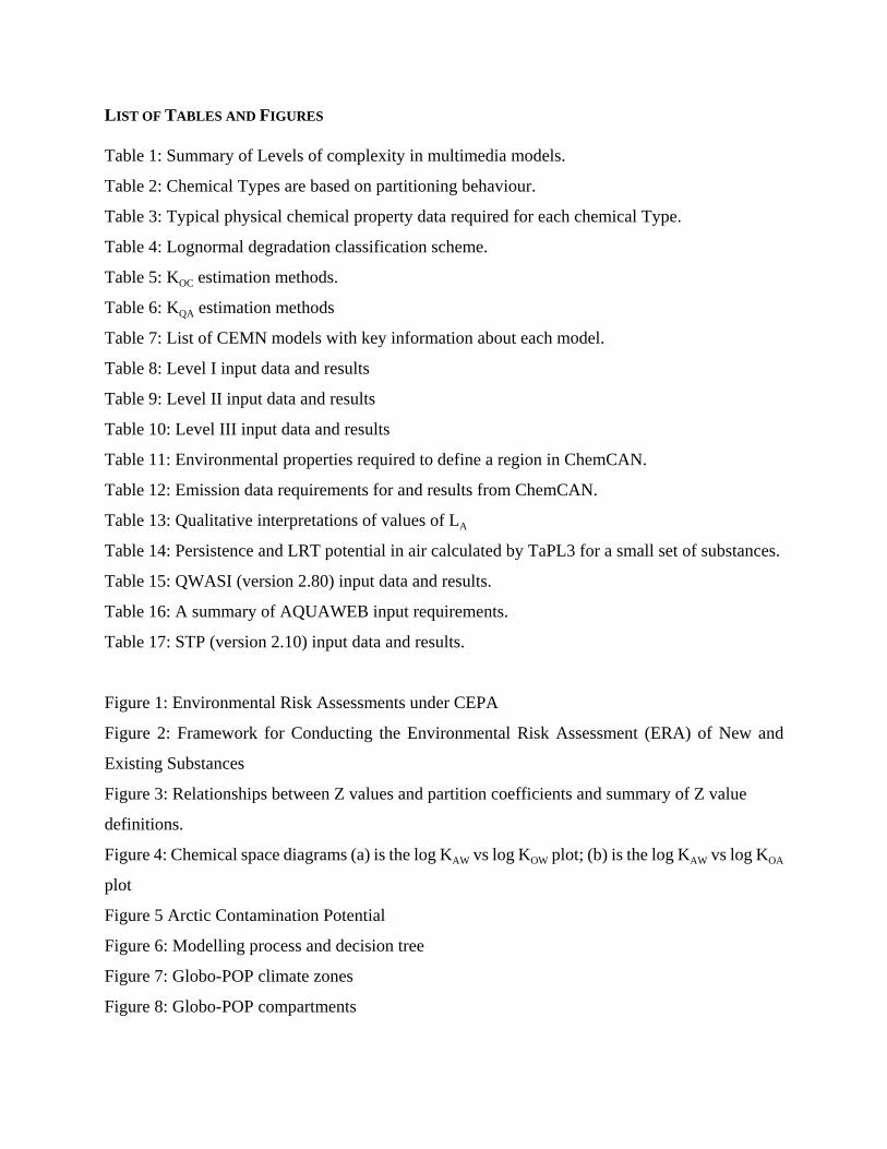
LIST OF TABLES AND FIGURES

Table 1: Summary of Levels of complexity in multimedia models.

Table 2: Chemical Types are based on partitioning behaviour.

Table 3: Typical physical chemical property data required for each chemical Type.

Table 4: Lognormal degradation classification scheme.

Table 5: KOC estimation methods.

Table 6: KQA estimation methods

Table 7: List of CEMN models with key information about each model.

Table 8: Level I input data and results

Table 9: Level II input data and results

Table 10: Level III input data and results

Table 11: Environmental properties required to define a region in ChemCAN.

Table 12: Emission data requirements for and results from ChemCAN.

Table 13: Qualitative interpretations of values of LA

Table 14: Persistence and LRT potential in air calculated by TaPL3 for a small set of substances.

Table 15: QWASI (version 2.80) input data and results.

Table 16: A summary of AQUAWEB input requirements.

Table 17: STP (version 2.10) input data and results.

Figure 1: Environmental Risk Assessments under CEPA

Figure 2: Framework for Conducting the Environmental Risk Assessment (ERA) of New and

Existing Substances

Figure 3: Relationships between Z values and partition coefficients and summary of Z value

definitions.

Figure 4: Chemical space diagrams (a) is the log KAW vs log KOW plot; (b) is the log KAW vs log KOA

plot

Figure 5 Arctic Contamination Potential

Figure 6: Modelling process and decision tree

Figure 7: Globo-POP climate zones

Figure 8: Globo-POP compartments

1

EXECUTIVE SUMMARY

This document is intended to assist the novice model-user in understanding when, why, and how touse models of chemical fate in the environment.

The complementary nature of monitoring and modelling are described and the role of each isoutlined. A key contribution of models is their ability to bring together knowledge about chemicalproperties, environmental properties, and processes. This facilitates understanding and can highlightknowledge gaps.

Models can be used to establish the entire mass balance of a substance as it is transported,transformed, and bioaccumulated in the environment. They thus enable estimations to be made ofcertain processes such as volatilization that can not be measure directly. Models can be used toestimate concentrations and fluxes as well as likely time trends in concentrations as a result ofchanges in emission rates or environmental conditions.

The regulatory background to model use in Environment Canada is described with a brief accountof similar approaches in other jurisdictions.

A basic description is provided of principles underlying the use of model, including processestreated, the fugacity concept, the benefits of applying models with increasing degrees or levels ofcomplexity and the contributions of steady-sate and dynamic models.

A six-stage process for general evaluations of chemicals is suggested and a number of more specificevaluations are described.

These topics result in a process for using models to establish a general understanding of thebehaviour of a chemical in the environment. The emphasis is on organic rather than inorganicchemicals.

The models developed by and available from Canadian Environmental Modelling Network aredescribed and detail is given on model selection and applications. No attempt is made to describemodels available from other organisations. The developers of these other models should beconsulted directly for information on the nature and applicability of their models.

A number of aspects relating to the interpretation of model results are described includinguncertainty, variability, sensitivity, validation, temperature effects, and steady-state and dynamictreatments.

Frequently asked questions are listed with answers and a full list of references is provided.

In total, this document is designed to provide the user, who is not necessarily experienced in modeluse, with guidance on the use of models for evaluation purposes.

-1-

1 INTRODUCTION

1.1 Background

This report is prepared as a part of the Contribution Agreement Development and Application ofModels of Chemical Fate in Canada”. It provides guidance on the use of the models in general andit specifically describes the models developed and distributed by members of the CanadianEnvironmental Modelling Network (CEMN).

1.2 Objectives

The objectives of this report are

• To give an overview of the science of fugacity-based models• To present a process for understanding the behaviour of a chemical in the environment• To provide familiarity with CEMN models• To give guidance on the use of CEMN models especially for the novice user

1.3 Outline

A brief outline of the regulatory background in Canada and around the world is provided.

This report provides basic instructions on the use and interpretation of the environmental fate modelsproduced by the members of the Canadian Environmental Modelling Network.

The role of models in understanding chemical fate in the environment is described including adiscussion of the complementary nature of modelling and monitoring.

The fugacity concept is explained and the mathematics of Level I, II, III and IV fugacity models isoutlined.

The six-stage process to understand chemical behaviour is described.

A listing of some of the models available from the CEMN is given with details on selected models.

Guidance is given on selecting a model, identifying input data sources, evaluating input data quality,and understanding model outcomes.

-2-

2 THE CANADIAN REGULATORY BACKGROUND

2.1 CEPA: The Canadian Environmental Protection Act

The Canadian Environmental Protection Act, 1999 (CEPA, 1999) is a statute that addresses theresponsibility of the Canadian Government to identify potential adverse effects on human health andthe environment from chemicals and other substances. CEPA, 1999 provides the federal governmentwith the authority to determine whether chemicals and other substances are “toxic” or capable ofbecoming toxic in the context of the statute. The Act also provides for a comprehensive“cradle-to-grave” management approach for chemicals and other substances.

2.1.1 Definition of substance

The Canadian Environmental Protection Act, 1999, requires the Ministers of the Environment andof Health to evaluate substances as defined in the Act and is considered key to the protection of theenvironment. CEPA, 1999 defines substances very broadly and under CEPA as:

“any distinguishable kind of organic or inorganic matter, whether animate or inanimate, and includes

(a) any matter that is capable of being dispersed in the environment or of beingtransformed in the environment into matter that is capable of being so dispersed or thatis capable of causing such transformations in the environment,

(b) any element or free radical,

(c) any combination of elements of a particular molecular identity that occurs in natureor as a result of a chemical reaction, and

(d) complex combinations of different molecules that originate in nature or are the resultof chemical reactions but that could not practicably be formed by simply combiningindividual constituents,”

and, except for the purposes of sections 66 (the Domestic Substances List), 80 to 89 (NewSubstances) and 104 to 115 (animate products of biotechnology), includes

“(e) any mixture that is a combination of substances and does not itself produce asubstance that is different from the substances that were combined,

(f) any manufactured item that is formed into a specific physical shape or design duringmanufacture and has, for its final use, a function or functions dependent in whole or inpart on its shape or design, and

-3-

(g) any animate matter that is, or any complex mixtures of different molecules that are,contained in effluents, emissions or wastes that result from any work, undertaking oractivity.”

2.1.2 Definition of CEPA toxic

CEPA 1999 requires the Minister of the Environment and the Minister of Health to assess substancesin order to determine whether the substance is toxic or capable of becoming toxic. Under the Act(Section 64), a substance is “toxic” if it is entering or may enter the environment in a quantity orconcentration or under conditions that:

(a) have or may have an immediate or long-term harmful effect on the environment orits biological diversity;

(b) constitute or may constitute a danger to the environment on which life depends; or

(c) constitute or may constitute a danger in Canada to human life or health.

Substances are assessed by the Ministers of Environment and Health, through the Existing and NewSubstances Programs jointly administered by Environment Canada and Health Canada.

2.1.3 Legislation for ecological risk assessment of existing substances

Substances assessed under the Existing Substances Program are broadly defined and primarilyincludes, but is not restricted to those substances found on Canada's original Domestic SubstancesList (DSL). The original DSL is defined under section 66 and specifies “all substances that theMinister is satisfied were, between January 1, 1984 and December 31, 1986,

(a) manufactured in or imported into Canada by any person in a quantity of not less than100 kg in any one calendar year; or

(b) in Canadian commerce or used for commercial manufacturing purposes in Canada.”

Substances on the original DSL may be given priority for risk assessment through the DSLCategorization Program (ESB 2003). As mandated under Section 73 (a) and (b) of CEPA, 1999,substances on the DSL are categorized as to whether they present to individuals the greatestpotential for exposure; or meet the persistence or bioaccumulation criteria, as satisfying theregulations (Canada Gazette, 2000) and are also inherently toxic. Those substances which meet theabove criteria will undergo a screening assessment under CEPA, Section 74.

Although the categorization of the substances on the DSL provides a major mechanism to identifysubstances of potential concern for the environment or human health and subsequent assessment,other substances may be identified for assessment through other mechanisms. Six other mechanismsfor substance identification are available and include those found through industry submitted data

-4-

(including CEPA, S.70); provincial or international decisions (CEPA, S. 75); public nominations;hazardous classes of substances identified through new substances notifications; emerging scienceand monitoring; and international assessment or data collection. The Minster is also responsible forcompiling a Priority Substances List (PSL) which the Minister considers a priority for riskassessment (CEPA S. 76(1)). Some substances may be exempt from assessment if the substance hasalready been adequately assessed under another Act of Parliament.

For each substance identified through the mechanisms above, the environmental risk assessmentapproach will generally follow closely with that described in this document, although somedeviations from the approach may occur depending on the purpose and type of assessment and/orthe type of substance being assessed. There are also general scientific reviews or investigations(CEPA, Section 68) or support to Ministers and Governor in Council (S. 90), or other scientificreviews for which the Existing Substances Program is responsible.

2.1.4 Legislation for ecological risk assessment of new substances

The New Substances Program is responsible for assessing substances that are defined, by exclusion,through the original DSL (Section 66). Substances that are “new” to Canadian commerce fall underthe purview of Parts 5 and 6 of the CEPA, 1999. New substances that are chemicals, polymers andinanimate products of biotechnology are covered in Part 5 of the CEPA, 1999, whereas Part 6 of theCEPA, 1999 deals with new substances that are animate products of biotechnology. This documentdoes not describe the approach for assessing the risk from products of biotechnology.

In CEPA 1999 the approach to the control of new substances is both proactive and preventative,employing a pre-import or pre-manufacture notification and assessment process. When this processidentifies a new substance that may pose a risk to health or the environment, the Act empowersEnvironment Canada to intervene prior to or during the earliest stages of its introduction to Canada.This ability to act early makes the new substances program a unique and essential component of thefederal management of toxic substances.

The assessment process begins when Environment Canada receives a New Substances Notificationprepared by the company or individual that proposes to import or manufacture a new substance oruse it for a Significant New Activity (SNAc). New Substances Notifications must contain allrequired administrative and technical data and must be provided to Environment Canada by aprescribed date before manufacture or import (Government of Canada, 1994). Notificationinformation is jointly assessed by the Departments of Environment and Health to determine whetherthere is a potential for adverse effects of the substance on the environment and human health. Thisassessment, which is considered a risk assessment, must be completed within a specified time, andwill reach a conclusion as to whether or not the substance is “toxic” under CEPA. A substance maybe notified several times under the New Substances Program depending on the volume of substancemanufactured or imported into Canada.

A substance assessed under the New Substances Program may receive several levels of assessmentdepending on the volume of the substance manufactured or imported into Canada, and whether the

-5-

New or Existing Substances

Existing Substances Program

NewSubstances Program

Mandated AssessmentsScreening Assessments (S. 74)PSL Assessments (S. 76)Review of other jurisdictions (S. 75)

Mandated AssessmentsNew Substances Assessment (CEPA S. 83)FDA Substances Assessment (S. 76)

Environmental Risk Assessment

CEPA Toxic?

No Further Actionunder these programs at this time

Risk Management Activities

Yes No

New or Existing Substances

Existing Substances Program

NewSubstances Program

Mandated AssessmentsScreening Assessments (S. 74)PSL Assessments (S. 76)Review of other jurisdictions (S. 75)

Mandated AssessmentsNew Substances Assessment (CEPA S. 83)FDA Substances Assessment (S. 76)

Environmental Risk Assessment

CEPA Toxic?





Yes No

substance is on the non-Domestic Substances List (NDSL). Substances notified at higher volumes(e.g., >5,000 kg/y) contain more information in the notification package and typically require a moredetailed assessment, while substances notified at lower volumes (e.g., <5,000 kg/y) often undergoonly a preliminary assessment.

The final levels of assessment must meet the higher information requirements of the schedules foundin the New Substances Notification Regulation (NSNR) (Government of Canada, 1994). Riskassessment conclusions of lower scheduled assessments may be different than those of the higherSchedules. This document describes the considerations and approaches used to prepare theenvironmental portion of the risk assessments.

The requirements for notification and assessment in CEPA 1999 do not apply if the new substanceis manufactured or imported for a use that is regulated under another Act of Parliament that requiresnotice and assessment (e.g., Pest Control Products Act). The Governor in Council is responsible fordetermining that another Act meets these requirements and for placing it on Schedule 2 of CEPA1999.

Figure 1 provides a schematic representation of how risk assessments for existing and newsubstances relate to the mandate of substance assessment under CEPA.

Figure 1: Environmental Risk Assessments (ERA) under CEPA

-6-

As the New Substances Notification Regulations are designed for commercial chemicals, a new setof regulations appropriate for the Food and Drugs Act products are being developed through theEnvironmental Assessment Unit (EAU) and the Office of Regulatory and International Affairs,Health Products and Food Branch.

2.2 The Precautionary Principle

Canada has a long-standing history of implementing the precautionary approach in science-basedprograms related to health and safety, environmental protection, and natural resources conservation.With the increasing emphasis on the adoption of this approach in decision-making, the federalgovernment has been working to develop a set of guiding principles to support consistent, credible,and predictable policy and regulatory decision-making across government when applying theprecautionary principle.

During the preparation of an environmental risk assessment, every effort will be made to incorporatethe precautionary principle to ensure that decisions are made with a precautionary perspective. TheCanadian Environmental Protection Act (CEPA), 1999, specifically addresses the importance ofapplying the precautionary principle in relation to the assessment and management of substances.In the preamble to the Act and in the introduction under Administrative Duties of the Governmentof Canada it states that “where there are threats of serious or irreversible damage, lack of fullscientific certainty shall not be used as a reason for postponing cost-effective measures to preventenvironmental degradation”. In addition, part V of CEPA, 1999, Section 76.1, which dealsspecifically with conducting and interpreting the results of a screening or PSL risk assessment, orthe evaluation of a decision from another jurisdiction, prescribes the application of the precautionaryprinciple through the statement that “Ministers shall apply a weight of evidence approach and theprecautionary principle when preparing and interpreting the results of assessments”.

Historically, and as described in this document, the application of the precautionary principle is andwill continue to be an integral part of the environmental risk assessment process. The applicationof the precautionary approaches in the environmental assessment is made through conservativeassumptions or quantitative adjustments for uncertainty regarding adverse fate or toxic effects to theenvironment or to adjust for the unknown or inaccurate exposure scenarios. As a practical example,in the effects assessment stages, a precautionary approach may manifest itself through the selectionof the lowest, most protective quantitative measurement or estimate from the available data, orthrough the application of conservative “assessment” factors which will lower the effectconcentration even more to account for data limitations. For the development of the exposurescenarios, precautionary assumptions are often applied through the assumption of large or maximumuse or release volumes and or, through the development of potential use or release scenarios.

2.3 Framework for the Environmental Risk Assessment (ERA) of Substances Under CEPA

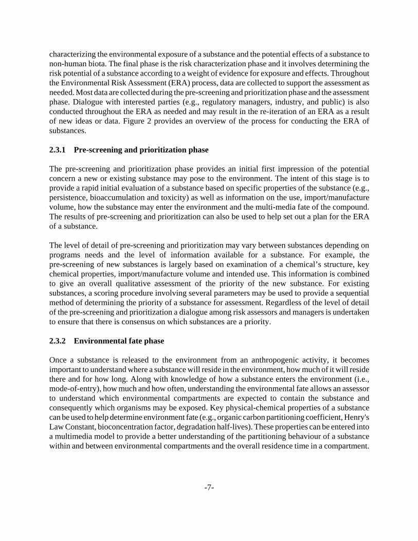
The environmental risk assessment of substances occurs through three main phases. The first phasecalled pre-screening and prioritization provides a means for triaging substances so that they may beprioritized for further assessment. The second phase, called the assessment phase, involves

-7-

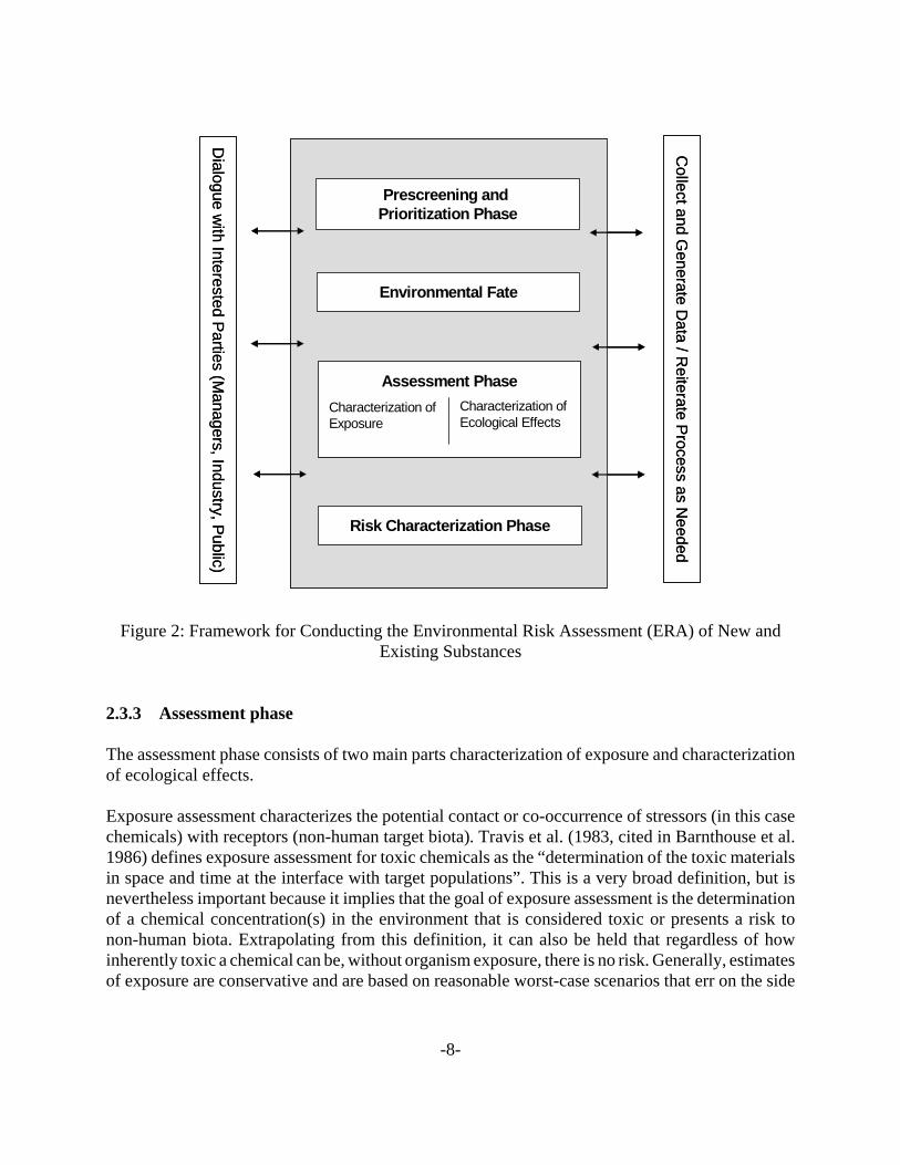
characterizing the environmental exposure of a substance and the potential effects of a substance tonon-human biota. The final phase is the risk characterization phase and it involves determining therisk potential of a substance according to a weight of evidence for exposure and effects. Throughoutthe Environmental Risk Assessment (ERA) process, data are collected to support the assessment asneeded. Most data are collected during the pre-screening and prioritization phase and the assessmentphase. Dialogue with interested parties (e.g., regulatory managers, industry, and public) is alsoconducted throughout the ERA as needed and may result in the re-iteration of an ERA as a resultof new ideas or data. Figure 2 provides an overview of the process for conducting the ERA ofsubstances.

2.3.1 Pre-screening and prioritization phase

The pre-screening and prioritization phase provides an initial first impression of the potentialconcern a new or existing substance may pose to the environment. The intent of this stage is toprovide a rapid initial evaluation of a substance based on specific properties of the substance (e.g.,persistence, bioaccumulation and toxicity) as well as information on the use, import/manufacturevolume, how the substance may enter the environment and the multi-media fate of the compound.The results of pre-screening and prioritization can also be used to help set out a plan for the ERAof a substance.

The level of detail of pre-screening and prioritization may vary between substances depending onprograms needs and the level of information available for a substance. For example, thepre-screening of new substances is largely based on examination of a chemical’s structure, keychemical properties, import/manufacture volume and intended use. This information is combinedto give an overall qualitative assessment of the priority of the new substance. For existingsubstances, a scoring procedure involving several parameters may be used to provide a sequentialmethod of determining the priority of a substance for assessment. Regardless of the level of detailof the pre-screening and prioritization a dialogue among risk assessors and managers is undertakento ensure that there is consensus on which substances are a priority.

2.3.2 Environmental fate phase

Once a substance is released to the environment from an anthropogenic activity, it becomesimportant to understand where a substance will reside in the environment, how much of it will residethere and for how long. Along with knowledge of how a substance enters the environment (i.e.,mode-of-entry), how much and how often, understanding the environmental fate allows an assessorto understand which environmental compartments are expected to contain the substance andconsequently which organisms may be exposed. Key physical-chemical properties of a substancecan be used to help determine environment fate (e.g., organic carbon partitioning coefficient, Henry'sLaw Constant, bioconcentration factor, degradation half-lives). These properties can be entered intoa multimedia model to provide a better understanding of the partitioning behaviour of a substancewithin and between environmental compartments and the overall residence time in a compartment.

-8-

Figure 2: Framework for Conducting the Environmental Risk Assessment (ERA) of New andExisting Substances

2.3.3 Assessment phase

The assessment phase consists of two main parts characterization of exposure and characterizationof ecological effects.

Exposure assessment characterizes the potential contact or co-occurrence of stressors (in this casechemicals) with receptors (non-human target biota). Travis et al. (1983, cited in Barnthouse et al.1986) defines exposure assessment for toxic chemicals as the “determination of the toxic materialsin space and time at the interface with target populations”. This is a very broad definition, but isnevertheless important because it implies that the goal of exposure assessment is the determinationof a chemical concentration(s) in the environment that is considered toxic or presents a risk tonon-human biota. Extrapolating from this definition, it can also be held that regardless of howinherently toxic a chemical can be, without organism exposure, there is no risk. Generally, estimatesof exposure are conservative and are based on reasonable worst-case scenarios that err on the side

Prescreening and Prioritization Phase

Environmental Fate

Risk Characterization Phase

Assessment PhaseCharacterization of Exposure

Characterization of Ecological Effects

Collect and G

enerate Data / R

eiterate Process as N

eeded

Dialogue w

ith Interested Parties (Managers, Industry, Public)

Prescreening and Prioritization Phase

Environmental Fate

Risk Characterization Phase





Collect and G

enerate Data / R

eiterate Process as N

eeded

Dialogue w

ith Interested Parties (Managers, Industry, Public)

-9-

of caution. The principles of pollution prevention under CEPA are implemented in the exposureassessment by examining all reasonably anticipated future uses and related exposures.

Effects assessment characterizes the type and magnitude of ecological effects resulting fromenvironmental exposure to a chemical or a combination of chemicals. Often, in risk assessments, themost sensitive receptor is used as the baseline from which to determine potential hazards to morethan one species. Often the type and magnitude of ecological effects is determined based onmeasurement endpoints (e.g., median lethal concentration, median effects concentration forreproduction). These endpoints correlate to the protection goals for the assessment (referred to asassessment endpoints) and are used to evaluate potential threats to populations of species in theenvironment. Ultimately, the effects assessment aims to derive the concentration of a substance inthe environment at which no effects are observable in target biota.

During the assessment phase, experimental and predicted data are collected or generated usingQSARs or environmental models. A re-iteration of the exposure or effects assessment may beundertaken if there is sufficient concern for the substance or new data have been supplied orcollected. As with the pre-screening and prioritization phase, dialogue with interested parties (e.g.,other assessors, managers, industry) is also performed to ensure that the characterization of exposureand ecological effects is based on the best available information.

2.3.4 Risk characterization

The risk characterization phase brings together the information from the exposure assessment andeffects assessment with the aim of concluding whether a substance poses a risk to non-human biota.The potential risk of a substance can be estimated using simple approaches such as the quotientmethod or can be based on several lines of evidence (e.g., PBT properties of a substance) for bothbiotic and abiotic endpoints.

The risk characterization phase also includes a qualitative assessment of the potential risk asubstance poses to the environment and will reach a conclusion on the toxicity of a substance asdefined under CEPA.

The risk characterization phase also points out where data gaps and uncertainties exist in theassessment and how these factors impact the quality of the assessment. A re-iteration of theassessment may be undertaken

2.4 The Need for a Multimedia Approach to Environmental Fate in ERA

In recent years, the characterization of uncertainty in ecological risk assessment has received muchattention and has become increasingly important regardless of the level of assessment performed.Tools for characterizing uncertainty range from relatively simple qualitative approaches to complexprobabilistic designs. The ecological risk assessment of new substances in Canada uses a screeninglevel approach. Characterization of uncertainty at the screening level becomes very importantbecause typically fewer data are available and used to estimate risk.

-10-

In 1998 and 1999 the New Substances Division of Environment Canada undertook two studies toexamine qualitatively the uncertainties associated with the exposure assessment of new substancesin Canada (BEC 1999a; BEC 1999b). In the first study, a characterization of the data gaps and shortcomings of the aquatic driven exposure assessment process was conducted. Specifically, acharacterization of the uncertainties associated with: (1) the estimation of release concentration, (2)fate and distribution, and (3) release, fate and distribution in non aquatic media was described. Oneof the key recommendations from the first study was that a multi media approach to conducting theexposure assessment of new substances in Canada was needed in order to address releases to mediaother than the water column. Although water column release and exposure form the basis fordetermining the predicted environmental concentration of a new substance, releases to other mediado occur and are appropriate (e.g., accumulation in soils) but are not routinely considered. In thesecond study, a strategy for dealing with the key data gaps and short comings that contribute toexposure uncertainty was detailed. In this study a preliminary approach to conducting the multimedia exposure assessment (MMEA) of new substances was outlined.

The New and Existing Substances Branches of Environment Canada have acted on the MMEArecommendation and strategy, which ultimately, led to the development of guidance for MMEA ofsubstances under CEPA (BEC 2001). Since 2001 many new multimedia tools and approaches havebeen developed. In particular, as the Existing Substances Program embarks on the risk assessmentof substances categorized as persistent or bioaccumulative and inherently toxic, EnvironmentCanada recognized the need for up to date and detailed guidance on multimedia models and theiruse in risk assessment. The result is this guidance document which is intended to be a evolving pieceof work that will be updated periodically as new techniques and understanding develop in the unitworld.

2.5 Practices in Other Jurisdictions

Practices in the US are generally similar to those in Canada in a scientific sense but the legislativeframework, the Toxic Substances Control Act, is different. Reference should be made to the USEPA,Office of Prevention, Pesticides and Toxic Substances for guidance on current practices.

Chemical assessment in Europe is conducted by the European Chemicals Bureau (ECB) located inIspra, Italy. This organization collects information on chemicals used in Europe and preparespriority lists. Priority substances are then allocated for assessment to specific member nations of theEuropean Union. Assessment reports are published and make recommendations on whether or notsome regulatory activity is deemed desirable. In recent years emphasis has been on “high productionvolume” chemicals. It is suggested that the reader consult the ECB website (http://ecb.jrc.it) fordetails of the assessment process (EUSES), priority lists, and technical guidance documents. Theassessment relies on the “SimpleBox” model developed by RIVM in the Netherlands.

Other national and international agencies also conduct assessments and provide guidance on modeluse, notably Japan, the OECD, and UNEP.

-11-

3 MODELS AS A CONTRIBUTION TO UNDERSTANDING ENVIRONMENTAL FATE

3.1 What models can do for you

When seeking to understand the behaviour of chemicals in the environment, there is a consensus thatit is no longer satisfactory to begin production and discharge before having some degree ofassurance of the absence of risk. This has been learned from the tragedies of the past as highlightedso elegantly by Rachel Carson (1962) in her book “Silent Spring”. Models provide a fast andinexpensive mechanism for bringing together the best of current science on chemical fate processesin the environment, with chemical properties data collected in the laboratory setting or from QSARs.

This should not be seen as excluding monitoring of in-use chemicals. For in-use and historic-usechemicals, monitoring and modelling should play complementary roles. In the modelling context,monitoring is critical for the continuing evaluation and improvement of the science on which themodels are based. Monitoring, in turn, benefits from the insights provided by modelling. Monitoringprograms contribute to the scientific understanding of environmental processes; better models aredeveloped; all with the ultimate benefit of improved chemical management.

As focus shifts from those substances already identified as problematic to a more preventive andprotective role, the weaknesses of existing science in explaining chemical behaviour becomeevident. For example, the models which have long been used for such substances as PCBs may notadequately describe fluorinated substances.

Historically, monitoring and modelling have primarily been conducted for the more populatedregions of North America and Europe. As global concern shifts from the immediate surroundingsof these affluent regions to the third world as a potential source and the polar regions as potentialdestinations for contaminants, new environmental processes become important. The effects oftemperature, snow fall, and ice cover require improved representation within the models. Monitoringand laboratory studies are required to facilitate the quantification of cold climate processes.

There are two fundamentally different types of models used in understanding chemical fate. The firstare statistical, knowledge-based models or correlations such as those contained in the EPIWIN suitewhere similarities in properties imply similarities in behaviour. The second are mechanistic, process-based models. Nearly all of the models developed by the CEMN are process-based models ofchemical fate.

Process-based models are a convenient way of bringing together the existing science in a simpleformat to calculate expected chemical behaviour. Models need to be continually tested for validityand challenged by monitoring programs and updated as the science existing at the time of modeldevelopment is shown to be inadequate for emerging chemicals or emerging concerns.

The models of the CEMN are founded upon the fundamental law that mass is neither created nordestroyed, and therefore, these models are known as “mass balance models”.

-12-

A mass balance environmental model can:

i) reveal likely relative concentrations, i.e., it is useful for monitoring purposes by indicatinglikely relative concentrations between media such as air, water, and fish.

ii) show the relative importance of loss processes, i.e., the process rates that we need to knowmost accurately

iii) link loadings to concentrations, i.e., identify key sources and ultimately their effects

iv) enable time responses to be estimated, i.e., how long recovery will take

v) generally demonstrate an adequate scientific knowledge of the system

Models are often not necessary when the sources, fate and effect are obvious, but they become morevaluable as situations become more complex, subtle, and with multiple sources. The user can alsoplay “sensitivity games” to determine what is most important and what is less important.

Models of the type described in this report can be used for the following general purposes.

i) to maximize our understanding of a monitored system.

ii) to obtain the best possible understanding of the likely behaviour of a substance not yet beingmonitored or not yet in production.

iii) to enhance a monitoring program by providing guidance on the likely behaviour of thesubstance of interest.

iv) to evaluate the results of a monitoring program and test for any systematic error in thechemical analysis, e.g., mis-reported units.

3.2 Environmental processes and pathways

There are three environmental processes or pathways to be considered in a mass balance model;transformation or degradation processes, advection processes that move the chemical out of themodelled system, and exchange processes between environmental media or compartments.

3.2.1 Transformation

A substance can be effectively removed from consideration by being transformed through achemical reaction. This is often described as degradation and first-order reaction kinetics areassumed in analogy with radioactive decay. These reactions include photolysis, oxidation,hydrolysis, and biodegradation.

-13-

Cautionary note: Our focus here is on the degradation of the original or “parent” chemical. The“daughter” product of any degradation reaction may or may not be more persistent,bioaccumulative, or toxic than the parent substance and thus may merit furtherinvestigation.

3.2.2 Advection

Advection processes such as wind transport and river currents can effectively remove a substancefrom the modelled system by transporting it to a different location.

Cautionary note: The substance may be more or less of a problem in the new location and thus may meritfurther investigation.

3.2.3 Intermedia exchange

Exchange between environmental media can occur by a multitude of processes including diffusion,rain dissolution, wet and dry aerosol deposition, runoff, and sedimentation and resuspension.Depending on the specific model other processes may be included. The importance of each processis highly dependent upon the chemical being investigated.

3.3 Fugacity concept

3.3.1 Origins, meaning, and usefulness

Fugacity was introduced by G.N. Lewis in 1901 as a criterion of equilibrium. It is similar tochemical potential, but unlike chemical potential, it is proportional to concentration.

Fugacity, which means escaping or fleeing tendency, has units of pressure and can be viewed as thepartial pressure which a chemical exerts as it attempts to escape from one phase and migrate toanother. In many respects, fugacity plays the same role as temperature in describing the heatequilibrium status of phases and in revealing the direction of heat transfer.

The application of the fugacity concept to environmental models is fully described in the text byMackay (2001).

When equilibrium is achieved a chemical reaches a common fugacity in all phases. For example,when the fugacity of benzene in water is equal to its fugacity in air, we may conclude thatequilibrium exists. However, these common fugacities will correspond to quite differentconcentrations. If the fugacity in water exceeds that in the air, benzene will evaporate until a newequilibrium is established.

-14-

The use of fugacity instead of concentration thus immediately reveals the equilibrium status of achemical between phases and the likely direction of diffusive transfer. Further, the magnitude of thefugacity difference controls the rate of transfer, by for example evaporation.

The relationship between fugacity (f, Pa) and concentration (C, mol/m3) is given mathematically inequation (1)

C = Zf (1)

where Z is a “fugacity capacity” or Z value with units of mol/m3 APa.

When performing fugacity calculations, the SI units of mol/m3 are used for all concentrations. It istherefore necessary to convert from mg/L for concentrations in water, or mg/kg or :g/g forconcentrations in solid phases. A knowledge of the density (kg/m3) of the solid phases is required.

3.3.2 Defining Z values

A Z value expresses the capacity of a phase, or environmental medium, for a given chemical. Zvalues are large when the chemical is readily soluble in a phase, i.e., the phase can absorb a largequantity of the chemical. A low Z value indicates that the phase can accept only a small quantity ofchemical, i.e., the chemical is “less-soluble” in the phase.

To establish Z values for each chemical in each phase, the process usually starts in the air phase. Inthe air, the Ideal Gas Law is applied.

PV = nRT (2)

where P is pressure, or fugacity in our case, V is the volume of the air, n is the number of moles ofthe chemical, R is the gas constant (8.314 PaAm3/molAK), and T is absolute temperature (K). SinceC = n / V, and C = Zf equation 2 can be re-written in fugacity terms as

ZA = 1/RT = CA /fA (3)

the subscript A referring to the air phase. ZA is thus about 0.0004 mol/m3APa for all chemicals in air.

A partition coefficient is the ratio of the concentrations in two environmental media at equilibrium,thus it is the ratio of the Z values of the two media. For example, the air-water partition coefficient,KAW, is

KAW = CA / CW (4)= ZAfA / ZWfW

and since KAW is measured when fA equals fW, i.e., at equilibrium,

-15-

KAW = ZA / ZW (5)

In general,

Ki,j = Zi / Zj (6)

Using the partition coefficients and previously calculated Z values, it is thus possible to calculateZ values for the chemical in other media such as soil, fish, and sediment if dimensionless partitioncoefficients are known.

Cautionary Note:Care must be taken to ensure that the partition coefficients are dimensionless becausemany are reported in dimensional units such as L/kg, i.e., a ratio of a solid phaseconcentration (mg/kg) to a liquid phase concentration (mg/L). The preferred units ofboth concentrations when calculating partition coefficients are mol/m3 or g/m3. Thisensures that the partition coefficient is dimensionless.

A very convenient and important description of chemical hydrophobicity or lipophilicity is KOW, theoctanol-water partition coefficient, which is the ratio of Z in octanol to Z in water. Octanol iscommonly used as a surrogate for lipids and organic matter in the environment. Hydrophobicchemicals such as DDT or PCBs have KOW values of about a million implying that ZO is about amillion times ZW, i.e., the water phase has a very limited capacity for the chemical. The chemicalis thus “water hating” or hydrophobic. KOW is used in correlations to describe partitioning fromwater into lipids of fish and other organisms and into natural organic carbon such as humic material.It is also used to correlate toxicity data for a variety of chemicals.

Correlations have been developed for several partition coefficients for organic chemicals as afunction of chemical properties such as solubility in water, KOW and vapour pressure. These can beexploited to give “recipes” for Z values. Caution must be exercised when using these correlationsfor chemicals of unusual properties such as ionizing acids or bases, detergents, dyes and polymers.Figure 3 is a summary of expressions which can be used to estimate Z values, detailed justificationbeing given in Mackay (2001). Notable is the use of KOW to estimate KOC the organic carbonpartition coefficient which is the key to the estimation of soil-water and sediment-water partitioncoefficients for many compounds.

Pure solutes are rarely present in the environment except as a result of chemical spills. The Z valuefor a pure solute is thus of more academic than practical interest. The fugacity of a pure solute is itsvapour pressure, PS (Pa). The concentration (mol/m3) is the reciprocal of the molar volume, v(m3/mol). It follows that Z is 1/(PS v).

-16-

Definition of Fugacity Capacities

Compartment Definition of Z, mol/m3 Pa

Air 1/RT R = 8.314 Pa m3 / mol K T = temperature, K

Water 1/H or CS/PS H = Henry’s law constant, Pa m3 / molCS = aqueous solubility, mol/m3

PS = vapour pressure, Pa

Solid Sorbent (e.g. soil,sediment, particles)

KP DS / H KP = solid-water partition coefficient, L/kgDS = density of solid, kg/L

Biota KB DB / H KB = biota-water partition coefficient, L/kg orbioconcentration factor (BCF), L/kgDB = density of biota, kg/L (often assumed to be 1.0 kg/L)

Pure Solute 1 / PS v v = solute molar volume, m3/mol

Figure 3: Relationships between Z values and partition coefficients and summary of Z value definitions.

H/RT or PS/RTCS or KAW

CS vAQUEOUS

SOLUBILITY

KOWOCTANOL-WATERPARTITION COEFF.

fFUGACITY

CAAIR

CPPURE

SOLUTE

COOCTANOL

CBBIOTA

CWWATER

CSSORBED

ZS = KPρS/H

ZA = 1/RT

ZO = KOW/H

ZS = KBρB/HZW = 1/H

= CS/PS

VAPOUR PRESSURE

PSv/RT

ρSKPρBKB

BIOCONCENTRATIONFACTOR

SORPTIONCOEFFICIENT

ZP = 1/PSv

AIR-WATER PARTITION COEFF.

-17-

3.4 An exploration of Levels

It is useful to explore the behaviour of a chemical in the environment through a series of models ofincreasing complexity. The simpler models are easiest to understand and have fewest datarequirements. As the complexity of the models increase, they become more challenging tounderstand and the data requirements increase. When more input data must be estimated, thereliability of the model output may become compromised. By stepping through a series of modelsof increasing complexity, understanding of the chemical’s behaviour can be maximized while thelikelihood of gross mis-representation is minimized.

Here the assumptions for the four levels of complexity are described. These calculations areembodied in a set of model software, each named for the level it contains, and in other software forspecific purposes. The software is described later.

3.4.1 Level I: simple equilibrium partitioning calculations

It is simplest to begin by assuming a closed environment with a constant amount of chemical presentat equilibrium between the environmental media. This “pop can” environment has no mechanismsfor chemical to be added or removed. There are no degradation or advection processes. There is noactive transport between environmental media; to return to the heat capacity analogy usedpreviously, the can has been on the shelf for long enough to have reached a constant temperature.In fugacity terms, this assumption of equilibrium means that a single fugacity exists in theenvironment, i.e., in a four-compartment environment where A is air, W is water, E is soil or “earth”,and S is sediment,

fA = fW = fE = fS = f (7)

A Level I model combines chemical partitioning (measured or estimated) data to give the Z valuesin each medium in the environment and, more importantly, the chemical’s partitioning tendency. Theinter-media surface areas are not needed because equilibrium is assumed between well-mixedvolumes of media.

The partitioning behaviour of a chemical can be most readily depicted and understood with achemical space diagram such as that shown later in Figure 4.

Some algebra M is total moles of chemical in the environment, Vi is volume, and Ci is concentration forcompartment i and all summations are over all i.

M = GViCi = GViZifi (8)

and since all fi are equal and can be designated f by equation (7)

M = f GViZi (9)

-18-

or

f = M / GViZi (10)

This is a Level I calculation.

The calculation sequence is• given the partition coefficients of a chemical, Z values can be determined• given compartment volumes, ZiVi can be determined• given an amount of chemical present, f can be determined from equation (10), and• from f, all concentrations, Ci = Zif and all amounts mi = Ci/Vi can be determined.As a final check, the sum of all mi must equal the total amount of chemical present.

A simple worked example for DDT in a water body such as a lake is given in Appendix D.

3.4.2 Level II: equilibrium partitioning with loss processes

The modelled complexity of the environment at equilibrium can be increased by including the lossprocesses of advection and degradation. Advection includes mechanical removal processes suchachieved by air and water currents and is characterized by a flow rate, G (m3/h). Degrading reactionscan include both chemical reactions and biologically-mediated degradation, and are characterizedby a half-life, J (h) or rate constant, k (1/h) = ln(2) / J. A set of transport or transformation valuesknown as fugacity rate constants or D values ( mol / Pa h ) are calculated as D = G Z or D = k V Zwhere V (m3) is the volume of the medium. Since the equilibrium assumption is maintained in LevelII calculations, there is no dependence on the medium to which the chemical is emitted; and totalemission into the environment is sufficient to describe chemical entry to this system. Again, theinter-media surface areas are not needed as equilibrium is assumed between well-mixed volumesof media.

Some algebra E is emission rate in mol/h

E = GDifi (11)

and by equation (7) and re-arranging equation (11)

f = E / GDi (12)

This is a Level II calculation.

The calculation sequence is• use the Z values from Level I• given compartment volumes, rate constants, and flow rates, all Di values can be determined

• for advection processes, A: DiA = Gi Zi

-19-

• for reaction processes, R: DiR = ki Vi Zi • given an emission rate, f can be determined from equation (12), and • from f, all concentrations, Ci = Zif and all rates Dif can be determined.As a final check, the sum of all loss rates Dif must equal the emission rate.

A simple worked example of DDT in a water body is given in Appendix E.

3.4.3 Level III: steady-state with multimedia transport

By removing the equilibrium assumption, the model complexity and data demands are againincreased. The steady-state assumption, i.e., the absence of change over time, is retained. Withoutthe equilibrium assumption the chemical’s fugacities in each medium generally differ and, it is nownecessary to describe active transport processes between environmental media. These can includeprocesses such as diffusion, volatilization, deposition, resuspension, and runoff and require a varietyof input data depending on the details of the environment modelled. For example, media volumesare no longer sufficient. The inter-media surface areas are needed to calculate many of these transferprocess rates. In general, D = A U Z where U is the transport velocity for the process in units of m/hand A is the area of the exchange surface in m2. Medium-specific emission rates, Ei, are nowrequired because the results are strongly dependent on the receiving medium or media, i.e., the“mode-of-entry”. This more complicated calculation will yield the same results as a Level IIcalculation if the chemical is rapidly transported between media such that all media have the samefugacity - the key assumption of Level II.

Some algebraEi are the emissions into each medium i, Di,j are the fugacity rate constants for chemical transferfrom medium i to medium j. Since chemical mass is conserved, the amount entering each mediummust equal the amount removed by either transport into another medium or by one of the lossprocesses of advection and degradation.

Entering = Advected + Degraded + Transferred (13)

Losses in medium i are given by

DiT = DiA + DiR + GDi,j (14)

Ei + GDj,i fj = fi DiT (15)

Note that GDj,i fj is the sum of the rate of input from other compartments j to compartment i.Re-arranging equation (15) gives

fi = ( Ei + GDj,i fj ) / DiT (16)

We thus obtain for n media, n equations with n unknown fugacities and we can solve them for allfugacities, from which concentrations, amounts and rates are calculated.

-20-

Note that we can have as many boxes as we like - the limitation is our ability to estimate D values,not computing power.

This is a Level III calculation.

The calculation sequence is• obtain the Z values from Level I, and DiA and DiR from Level II• given the necessary transfer process information, calculate all Di,j• given all emissions, Ei, the set of mass balance equations (16) will yield the set of fugacities,

and • from all fi, all concentrations, Ci = Zif and the total removal rate from the environment

G(DiAfi + DiRfi) can be determined.As a final check, the total removal rate must equal the sum of the emission rates, GEi and eachcompartment should also display a mass balance with inputs equalling outputs.

A simple worked example for DDT in a water body is given in Appendix F.

3.4.4 Level VI: dynamic

This next level of complexity, Level IV, includes change over time, i.e., it does not assume steady-state. Here a single emission such as a spill may be followed through time, or the effect of emissionreductions examined in detail. Sufficient input data is often difficult to obtain and erroneousestimates can lead to false conclusions. Thus, it is important to follow a progression of increasingmodel complexity and data demands to anticipate the likely dynamic behaviour prior to performingsuch calculations.

Some algebra and some calculus

For a time-varying emission to medium i, Ei(t), mass balance dictates that all chemical enteringmedium i must be accounted for through transport into another medium or by one of the lossprocesses of advection and degradation or must become a part of the inventory of chemical inmedium i. Thus the amount of chemical in medium i at time t is given by

mi(t) = mi(t-1) + )t dmi/dt (17)

dmi/dt = d(fi Vi Zi)/dt = rate of chemical entering - rate of chemical leaving (18)

or assuming volumes and Z values are constant

Vi Zi dfi/dt = Ei(t) + GDj,i(t) fj(t) - fi(t) DiT(t) (19)

In equation (19) the left-hand side is the inventory change and the terms on the right-hand side aredirect emission to the compartment, transport to the compartment, and losses from the compartment.

-21-

DiT it the total of all loss D values by reaction, advection, and intermedia transport. A dynamiccalculation for constant emissions, if continued for a long enough period, will achieve the steady-state condition and results will be equivalent to those from the Level III calculation.

There are thus n simultaneous linear differential equations. They can be solved analytically but itis often easier to solve them by numerical integration. The result is the time-course of concentrationsin each medium.

3.4.5 Summary of Levels

Table 1: Summary of Levels of complexity in multimedia models

Level Assumptions

I Closed systemDefined chemical amountEquilibrium between media ==> one fugacity

II Single chemical emission rateReaction and advective loss processesEquilibrium between media ==> one fugacity

III Chemical emission rates and mode-of-entryReaction and advective loss processesNon-equilibrium between media ==> different fugacitiesSteady-state system, i.e., unchanging with time

VI Dynamic system, i.e., changing with time

3.5 A Six-Stage Process to Understanding Chemical Fate

In 1996, Mackay et al (1996a) outlined a 5-stage process to understand the behaviour of a substancein the environment. The five stages are: (1) chemical classification, (2) acquisition of discharge data,(3) evaluative assessment of chemical fate, (4) regional or far-field evaluation, and (5) local or near-field evaluation. A sixth stage was suggested by MacLeod and Mackay (1999) in which an exposureevaluation would be conducted.

Recently, in recognition of the challenges of obtaining the emission data for stage 2, it has beensuggested that target emissions can be calculated from critical concentrations to evaluate risk. Amore detailed discussion of this risk evaluation is given later.

This process generates an increasing understanding of the chemical of interest. Often sufficientinformation will be generated early in the process and the final stages will be unnecessary, or allowsimplifying assumptions to be made without loss of accuracy. For example, when gathering the datafor stage 1, it may become evident that the substance is not multimedia in nature but partitions

-22-

exclusively to only one or two environmental media. In such a case, the degradation half-lives in themedia to which it does not partition may be assumed to be infinite (i.e., the rate is zero) and do notneed to be measured or estimated.

This gradual increase in data requirements and complexity facilitates the mental assimilation of theinformation generated. By plotting the partitioning properties of a substance much may be learned.By calculating the substance’s fate in an evaluative environment, key processes can be identified.

It is argued by some that all the information may be generated by using a single, complex andrealistic model. This assumes that all of the required input data are available. It assumes that all theprocess information encoded in the model is correct and applicable. It assumes that the greatestrealism is always required and that the results will always be interpretable.

It is well-established that as models increase in realism and complexity, the data demands increase;data demands that are often impossible to satisfy except through estimation methods. As more inputdata are estimated, the reliability of the results becomes compromised. Also, as the complexity ofthe model increases, the results become more challenging to interpret and thus more prone to mis-interpretation.

For these reasons, we recommend that simpler models be applied first and the complex models onlyused when necessary.

3.5.1 Stage 1: Chemical classification and physical data collection

PartitioningFor convenience in modelling, three chemical types have been defined (Mackay et al, 1996a). thisallows these chemicals to be treated by multimedia models such as those developed by the CEMN.The defining characteristics and some examples are given in Table 2. Table 3 gives the typicalproperty data required for a chemical of each defined type. Data sources and estimation methods aresuggested later in this section.

Occam's razor or the Principle of ParsimonyEssentia non sunt multiplicanda praeter necessitatem

"What can be done with fewer (assumptions) is done in vain with more"

-23-

Table 2: Chemical types are based on partitioning behaviour.

Type Partitionsinto

Z Equilibriumcriterion

Examples

1 all media non-zero inall media

fugacity most organic chemicals (e.g.,chlorobenzenes, PCBs) includingionizing chemicals

2 not air . or = 0 inair

aquivalence cations, anions, involatile organicchemicals, and surfactants

3 not water . or = 0 inwater

fugacity very hydrophobic compounds (eg.,long-chain hydrocarbons, silicones)

4 not air andnot water

. or = 0 inair and water

none polymers

5 speciating chemicals (e.g., mercury)

Type 4 substances tend to remain in their original state as a solid in the environment thus modellingof the type described in this document does not serve a useful purpose. It should be noted thatpolymers may contain unreacted monomer and other additives such as plasticisers that are ofpossible concern. These substances may degrade to form other chemicals that can have adverseeffects.

Type 5 substances display complex environmental fate and require case-specific evaluation.

Table 3: Typical physical chemical property data required for each chemical type

Type Data required

1 molar mass, data collection temperature, solubility in water, vapour pressure, andoctanol-water partition coefficient (KOW) and possibly pKa

2 partition coefficients from solids or organic carbon to water

3 partition coefficients from solids or a pure phase to air

AquivalenceThe Z values for Type 2 chemicals are calculated using the aquivalence approach (Mackay 2001).Since the vapour pressure and the air-water partition coefficient may be zero, Z for water becomesinfinite if calculated as for Type 1. Therefore, calculation starts by defining Z for water as 1.0. Allother Z values are deduced from the Z value for water and the partition coefficient of the phase withrespect to water.

-24-

Ionizing Chemicals

Organic acids and bases such as phenols, carboxylic acids, and amines, may dissociate or ionize inthe environment. As a result of this tendency to dissociate an acidic substance may exist in its non-ionic protonated or neutral form and its ionic de-protonated, or charged, form. Bases behavesimilarly but the protonated form is charged. These forms have different properties, for example theneutral form may evaporate from water, but the ionic form does not evaporate. It is thus essentialto calculate the fractions in each form.

The simple, first order approach of Shiu et al (1994) and Mackay et al (2000) to quantifying thesefractions is briefly described below.

The neutral form of an acid molecule can be designated RH where R is an organic moleculecomprising carbon, oxygen, hydrogen and possibly sulfur, nitrogen and phosphorus. When dissolvedin water, the molecule may ionize to form hydrogen ion H+ and an anion R-

RH 6 R- + H+

The molecule may have several hydrogens that can dissociate. No correction is made for the effectof cations other than H+. It is assumed that dissociation takes place only in aqueous solution, not inair, organic carbon, octanol or lipid phases. Some ions and ion pairs are known to exist in the lattertwo phases, but there are insufficient data to suggest a general procedure for estimating quantities.

The dissociation constant is defined as follows.Ka = [R-] [H+] / [RH] (20)

so pKa = log ([R-] [H+] / [RH]) (21)

Typical values of pKa for chlorinated phenols range from 4 to 8. It is the relative magnitudes of pKaand pH, the environmental acidity, that determine the extent of dissociation.

Rearranging equation (20) gives

log ( [R-] / [RH] ) = log I = - log [H+] + log Ka (22) = pH - pKa

where I is the ratio of the ionized to non-ionized concentrations, pH is -log [H+] and pKa is -log Ka.Note that base 10 logarithms are used. This leads to the Henderson Hasselbalch equation

I = 10 (pH - pKa) (23)

Note that if the substance has several pKa values, the one corresponding to the primary or firstdissociation process should be used. This has the lowest value of pKa. For example, if values of 5,8 and 11 are given, use 5 and ignore the others, at least for screening purposes.

-25-

x IN dd= +1 1/ ( )

Z I ZI e Ne e=

IdpH pKad= −10( )

Z Z ZT N Ie e e= +

x I II d dd= +/ ( )1

Z x ZN N Td d d= ×

Z x ZI I Td d d= ×

Z Z x ZN N N Te d d d= = ×

Assuming a pH of 7.0 and that the ionic form does not evaporate from water, sorb to organic matter,or bioaccumulate into lipids, this ratio is assumed to apply in all water phases in the environment.

As a result of ionization, there can be ambiguity about the values of the solubility in water and KOW.If experimental data are used, the pH should also have been specified to clarify if the properties arethose of the non-ionised or non-ionised plus ionised forms. If the latter applies, the solubility andKOW of the non-ionised form can be calculated. If the data are from an estimation method, the valuesgenerated will correspond to the molecular structure provided to the method. For example, aSMILES notation used in QSARs will normally refer to the non-ionised form, not the ionised form

Models treating ionizing chemicals normally require the solubility of neutral species either from anestimation method or measured.

For the general case of a pKa measured at an acidity of pHd, where the subscript d represents thedata pH, the ionic to non-ionic ratio at of pHd is

(24)thus the non-ionic fraction is

(25)and the ionic fraction is

(26)

The for both species in water at the pH of the data collection is 1/Hd, therefore the Z for theZTd

ionic fraction is (27)

Similarly the Z for the non-ionic fraction is

(28)

But, the Z for the non-ionic fraction is unaffected by the pH of the water and therefore, at the pH ofthe environment (e) is given by

(29)

The Z for the ionic fraction, at the pH of the environment, is given by

(30)

And finally, the Z for both species together, at the pH of the environment, is

(31)

-26-

To calculate the D values for the loss and transfer processes care must be taken to use the Z valuerelating to the species participating in the process.

The same arguments apply to bases. Rather than use the constant Kb it is usual to express it also asKa, noting that pKa + pKb = 14.

Note that in the Handbook by Mackay et al (2000) the aqueous solubilities selected are primarilythose of the non-ionic form.

Degradation

Chemical transformation, or degradation, can be considered to be the decomposition of the substanceof interest into water, carbon dioxide, and inorganic compounds, however, only primary degradation,i.e., the degradation causing a change in the identity of the substance, is considered here. Thedaughter compounds are normally considered separately from the parent compound as they have acompletely different set of properties, including a different toxicity, and thus a different priority.

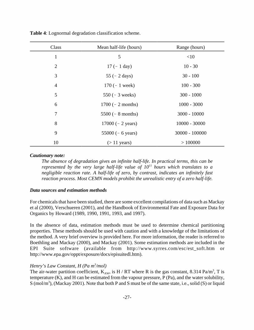
Degradation is normally characterized as a first-order reaction and quantified by a reaction rateconstant, ki (1/h), or a half-life, Ji (h) = ln(2)/ki in each environmental medium, i. Degradation occursby processes such as photolysis, hydrolysis, oxidation and biodegradation. The rates of theseprocesses are strongly dependent upon environmental conditions such as temperature, solarinsolation, and the nature and activity of the microbial community. Thus degradation data arecharacterized by a high inherent variability. For a more detailed discussion of natural variation indegradation half-lives consult Boethling and Mackay (2000) or Webster et al (1998). Variousresearchers have sought to acknowledge this variability by defining degradation classes andincluding a range of values in each class. For example, Syracuse Research Corporation (SRC), usesan semi-quantitative scheme based on designations of hours (4.1 h) , hours to days (30 h), days (56h), days to weeks (208 h), weeks (360 h), weeks to months (900 h), months (1440 h), and“recalcitrant” (3600 h) ( ref ). Another is the lognormal classification scheme of Mackay et al (2000)and Webster et al (2003) as shown in Table 4.

-27-

Table 4: Lognormal degradation classification scheme.

Class Mean half-life (hours) Range (hours)

1 5 <10

2 17 (- 1 day) 10 - 30

3 55 (- 2 days) 30 - 100

4 170 (- 1 week) 100 - 300

5 550 (- 3 weeks) 300 - 1000

6 1700 (- 2 months) 1000 - 3000

7 5500 (- 8 months) 3000 - 10000

8 17000 (- 2 years) 10000 - 30000

9 55000 (- 6 years) 30000 - 100000

10 (> 11 years) > 100000

Cautionary note: The absence of degradation gives an infinite half-life. In practical terms, this can berepresented by the very large half-life value of 1011 hours which translates to anegligible reaction rate. A half-life of zero, by contrast, indicates an infinitely fastreaction process. Most CEMN models prohibit the unrealistic entry of a zero half-life.

Data sources and estimation methods

For chemicals that have been studied, there are some excellent compilations of data such as Mackayet al (2000), Verschueren (2001), and the Handbook of Environmental Fate and Exposure Data forOrganics by Howard (1989, 1990, 1991, 1993, and 1997).

In the absence of data, estimation methods must be used to determine chemical partitioningproperties. These methods should be used with caution and with a knowledge of the limitations ofthe method. A very brief overview is provided here. For more information, the reader is referred toBoethling and Mackay (2000), and Mackay (2001). Some estimation methods are included in theEPI Suite software (available from http://www.syrres.com/esc/est_soft.htm orhttp://www.epa.gov/oppt/exposure/docs/episuitedl.htm).

Henry’s Law Constant, H (Pa m3/mol)The air-water partition coefficient, KAW, is H / RT where R is the gas constant, 8.314 Pa/m3, T istemperature (K), and H can be estimated from the vapour pressure, P (Pa), and the water solubility,S (mol/m3), (Mackay 2001). Note that both P and S must be of the same state, i.e., solid (S) or liquid

-28-

(L). That is, H = PL / SL or H = PS/SS. For substances with a melting point greater than 25 /C, i.e.,solids at room temperature, a fugacity ratio, F, can be defined from the melting point, MP, and thetemperature at which PS was measured (normally about 25 /C).

F = e (6.79 x (1-MP/T) (32)The sub-cooled liquid vapour pressure, PSL is then PS / F and H = PSL / SL

Organic Carbon Partition Coefficient, KOC (L/kg)The organic carbon - water partition coefficient, KOC (L/kg), can be estimated from either KOW, orthe water solubility, S.

Table 5: KOC estimation methods

Estimation Source

KOC (L/kg) = 0.41(kg/L) KOW Mackay 2001

KOC (L/kg) = 0.35(kg/L) KOW Seth et al 1999

equations of the form log KOC = a log KOW + bwith various values of a and b

Boethling and Mackay 2000p153 Table 8.1

equations of the form log KOC = a log S + bwith various values of a and b

Boethling and Mackay 2000p154 Table 8.2

Soil and Sediment - Water Partition CoefficientsThe partitioning between the solid fraction of soil or sediment, and water, can be obtained as ameasured equilibrium partition coefficient, Kp (L/kg) = CS (mg/kg) / CW (mg/L). Using the densityof the solids, a dimensionless partition coefficient can be determined. For example, for soil,

KSoil Solids, Water = Kp (L/kg) DSoil Solids (kg/m3) / (1000 L/m3) (33)where DSoil Solids is the density of soil solids and 1000 L/m3 is a volumetric conversion.It is also possible to estimate Kp from KOC as

Kp (L/kg) = y KOC (L/kg) (34)where y is the mass fraction of organic carbon present in the soil solids (i.e., dry soil) (Boethling andMackay 2000; Mackay 2001). There are four assumptions that must apply to use this estimationmethod, otherwise Kd should not be estimated using this equation.- 1 - sorption is exclusively to the organic component of the soil (or sediment)- 2 - all soil (or sediment) organic carbon has the same sorption capacity per unit mass- 3 - equilibrium is observed in the sorption-desorption process- 4 - desorption isotherms are identical.

-29-

Aerosol - Air Partition CoefficientAerosol - air partitioning is not normally measured for evaluation purposes. It can be measured inthe environment by measuring concentrations in air before and after filtration. It is variouslyestimated as shown in Table 6.

Table 6: KQA estimation methods

Estimation Source

KQA = 6 x 106 / PL Mackay 2001

Kp (m3/:g) / KOA = B where B is b × 10-12 thusKQA = KOA ×DQ (kg/m3) × b × 10-3 (m3/kg)b is approximately 1.5 for most persistent organics

Finizio et al 1997

logKp = (a * logKOA) + b orKQA = KOA

a ×DQ (kg/m3) ×10 ( b + 9) (m3/kg)a is approximately 0.55 and b is -8.23 for most persistent organics

Finizio et al 1997

log KP (m3/:g) = log KOA -12.61 orKQA = KOA ×DQ (kg/m3) × 10-3.61 (m3/kg)

Bidleman and Harner,2000

Due to the small volume of aerosols present, the amount of chemical sorbed is small. For substanceswith a high KOA, the concentration may be high and scavenging may be an important transport vectorfor removal of the substance from the air. For low KOA substances, partitioning to aerosols isrelatively unimportant. When KOA is very large, i.e., 1010 and above, most chemical in theatmosphere is likely to be sorbed to aerosols. Benzo[a]pyrene is an example.

Biota - Air and Biota - Water Partition CoefficientsPartitioning between the abiotic and biotic media in the environment is not normally measured.Partitioning between biota (B) and the air or water is usually estimated assuming partitioning to onlythe lipid fraction. If this assumption is not true, some other estimation method should be used. Foraquatic biota such as fish, if a lipid fraction of 0.05 is assumed, then the partitioning coefficient, KBW= 0.05 KOW. Similarly for vegetation, if the leaves are assumed to have a lipid fraction of 0.01, theleaf-air partition coefficient, KBA = 0.01 KOA. For roots, a root-water partition coefficient may beestimated in the same way.

DegradationAs for chemical partitioning properties, there is a variety of data sources including those listedabove. Specific to degradation data is the Handbook of Environmental Degradation Rates (Howard,1991). Estimation methods have also been developed. A review of existing methods and suggestionsfor their application are given in a companion document to this report (Arnot et al, 2005). Somee s t i m a t i o n m e t h o d s a r e i n c l u d e d i n t h e E P I S u i t e s o f t w a r e(http://www.epa.gov/opptintr/exposure/docs/episuite.htm).

-30-

Toxicity

It is important to identify the potential for concern regarding the toxicity of the substance. If asubstance is unlikely to have toxic effects at the expected concentrations, it may not warrant furtherinvestigation. A substance with a higher probability of toxic effects should be investigated first, andmore fully.

To a first approximation there are three methods of expressing toxicity.

First is to define a concentration external to the organism that will cause a specified effect such aslethality of failure to reproduce. The aquatic LC50 and the occupational Threshold Limit Value(TLV) in air, applicable to occupational exposure, are examples.

Second is a dose, often expressed in mg/kg body weight per day, which causes an effect. This iswidely used in human toxicology. The dose may be the product of a concentration in food and thequantity of food consumed per day.

Third is the delivered dose or the internal concentration or quantity or critical body residue ofchemical causing the effect. For example, a chemical that exerts toxicity by narcotic or baselinetoxicity does so at a concentration in the body of 1 to 5 mmol/kg body weight. The concentrationmay also be in a specific tissue within the organism. Generally, chemicals which have similar modesof toxic action have similar internal concentrations at the same effect level. Obviously thecalculation of this concentration requires a bioaccumulation or even a pharmacokinetic model.

The issue evaluating toxicity is beyond the scope of this Guidance but it is useful for the modellerto know how the results are to be used in the evaluation of toxic effects. Many believe that the futureof environmental toxicology lies in calculating the third metric of toxicity, namely the critical bodyresidue required to cause the specified mode of toxic action. The mode of action can, in principle,be predicted from molecular structure.

3.5.1 Stage 2: Acquisition of discharge data

This is typically a very challenging task. For many substances of concern, discharges are dispersedand highly population and culturally dependent. The components of automobile exhaust are typicalof this group of substances. At the other extreme are substances discharged at point-sources, oftenindustrial in nature. Where such discharge data exist they may be incomplete or suited only local-scale evaluations.

-31-

3.5.2 Stage 3: Evaluative assessment of chemical fate

Armed with the data collected in stages 1 and 2 of this 6-stage process, modelling is now bothpossible and useful. An examination of the behaviour of the substance in a generic or “evaluative”environment increases our understanding without requiring regional properties and in a way that canbe compared across regulatory jurisdictions. This can be preformed with a models such as the 3-partset Level I, Level II, Level III or the EQC model that combines the calculations of the other threebut with less flexibility for the user. (See Section 4.3.1 to 4.3.4 for details on these models.) For anevaluative assessment a unit amount or rate of emission can be used as absolute concentrations arenot the focus of this stage of the six-stage process.

The area for an evaluative assessment should be large enough that wind dispersion does notdominate the distribution of concentrations to the exclusion of all other information. In the EQCmodel an area of 1011 m2 or105 km2. This is about the size of southern Ontario or twice the size ofNova Scotia. This is large enough to show chemical exchange behaviour in the environment. If asarea on the order of a few kilometres square is used, local sources and wind patterns will dominateand a dispersion model should be used. One can consider two extremes of scale, for very small areaslosses are entirely dominated by advection but for the entire globe degradation losses dominate.Degradation and advection losses become equal when the reaction half-life is similar to theadvection residence time. The smaller value dominates since it reflects a faster process.

In the Level I calculations, the partitioning properties of a chemical are used to show theenvironmental media in which it will tend to be present. The term “realistic presence” has been usedto designate an amount of at least 5% in an environmental medium (Webster et al 2004a; Woodfineand Mackay 2001; Environment Canada 2003). A multimedia chemical is realistically present inmore than one environmental medium. For single-medium chemicals, i.e., chemicals with a realisticpresence in only one medium, multimedia models are neither needed nor useful. The fate of a single-medium chemical is limited to processes occurring solely in that medium (advection anddegradation). Multimedia models should only be used if the chemical is realistically present in atleast two environmental media.

The “realistic presence” concept has been suggested as a rational method of avoiding demands fordata which prove to be of little or no value. If a chemical is present only to the extent of say 2% ina medium it is unlikely that the overall fate of the chemical, especially its persistence, will beaffected by rates of degradation in that medium. It can thus be argued that no degradation rate dataare needed and a zero degradation rate (infinite half-life) can be assumed. The 5% cut-off has beenestablished by experience but is somewhat arbitrary. (Woodfine and Mackay 2001, Webster et al2004a).

In the Level II calculations, the partitioning and degradation properties of a chemical are combinedto give a first estimate of the relative importance of each removal process, and the longevity orpersistence (P) and long-range transport potential (LRT) of the chemical. While current Level IImodels do not explicitly calculate LRT it can be calculated manually as the product of an assumedwind speed (km/h), the overall residence time of the chemical (h), and the ratio of the amount in air

-32-

to the total amount in the system. The values of P and LRT should be considered in the context ofthe values for ranking against other chemicals. The absolute value P and LRT calculated by thesemodels are not meaningful.

For multimedia chemicals that are not realistically present in at least two media as identified in theLevel I calculations, the same simplifying assumptions regarding the degradation data requirementsfor Level II calculations may be made. For example, if a chemical does not partition appreciably intoair, the degradation half-life in air can be assumed to be infinite, i.e., assume no degradation of thechemical in a medium in which it is not present. This assumption represents a reduction in the datarequirements while having a minimal impact on the model results (Woodfine and Mackay 2001,Webster et al 2004a, Environment Canada 2003).

In a Level III calculation, the partitioning and degradation properties of the chemical are combinedwith intermedia transport process information. In the absence of the equilibrium assumption, therelative emission rates to each environmental medium becomes essential information because theresults are often strongly dependent on the mode-of-entry. It is common practice among researchers,when these relative emission rates are not known, to perform a separate Level III calculation for aunit emission into each potential receiving medium and focus on the worst-case scenario. Thus ifthere are three potential receiving media, the calculations are performed three times, once for eachmedium as receiving a unit emission. The results of the three scenarios are compared and theassessor can then focus on the worst-case, e.g., the unit emission to air. Identifying the worst-casescenario will require a knowledge of the target organism and exposure routes. Of course, if emissionmode-of-entry data are available they should be used.

From the Level III model and using the evaluative environment the relative importance of eachtransport and removal process can be ascertained for the chemical and emission scenario underinvestigation. The importance of each process is chemical and emission scenario dependent and cannot be determined in a general way. Consider for example, a chemical with a high KOA emitted toair. This chemical will sorb strongly to aerosols and wet and dry aerosol deposition will beimportant. Rain rate will be important as it affects the rain scavenging of this aerosol-associatedchemical. The dissolved fraction of the rain deposited fraction of chemical will be relatively lessimportant and depends on the KAW of the chemical.

Level III calculations also provide values for P and LRT. When the relative emission rates to eachenvironmental medium are known, this represents an improvement on the estimate provided by theLevel II calculations. It is not yet clear that there is any benefit from these estimates of P and LRTwhere the relative emission rates are not known, at least with some degree of confidence. The valueof LRT is, again, not meaningful in an absolute sense but should be compared to the values for otherchemicals to provide a ranking. The value of P, while meaningful, may also usefully be comparedbetween chemicals.

Finally, Level III calculations using an evaluative environment can be compared to monitoredconcentration data. This must be done with some care and acknowledging the inherent error that willbe caused by the properties of the evaluative environment not matching those of the region where

-33-

the data were collected. There are some advantages to this pseudo-regional modelling. First,monitoring data from a variety of regions can be combined. For example, much of the northern US,southern Canada, and western Europe all have somewhat similar environments. Thus whenmonitoring data are sparse, data from all of these regions can be combined and the model resultscompared to the range of monitored values. It is of particular interest to compare the relativeconcentrations, that is, if the monitored concentration in the soil samples is ten times that of thewater samples, is this seen in the model results? This type of comparison may point to selectivesampling where only locations of high concentration need be monitored.

3.5.3 Stage 4: Regional or far-field evaluation

Regional or far-field evaluations with region-specific environmental properties provide the first setof concentrations for direct comparison to monitoring data collected in a specified area such asSouthern Ontario, or Northern BC.

The ChemCAN model was developed for this purpose and contains a database of properties for 24regions of Canada. For consistency and comparison the database also contains the standard EQCenvironment.

As for an evaluative assessment, a region should be defined as an area large enough that winddispersion does not dominate to the exclusion of all other information. Local hot spots are nottreated. It is important when defining a region for this stage in the process to specify an area largeenough that advective flow-through will not dominate the chemical removal processes such that allintermedia and degradation effects are obscured. In ChemCAN the Canadian regions range in sizefrom 2176000 km2 for the Arctic and North Nunavut region to 80190 km2 for the B. C. - SouthPacific Maritime region. This is large enough to show chemical exchange behaviour in theenvironment. If as area on the order of a few kilometres square is used, local sources and windpatterns will dominate and a dispersion model should be used. A region should not be defined withan area of less than about 100 km by 100 km, or 10000 km2.

Using too large an area will also lead to erroneous results as the assumption of a single well-mixedair compartment will be violated. As a general rule, the area should not be greater than about 1000km by 1000 km or 1000000 km2. Larger areas should be sub-divided and each section consideredseparately with wind and river currents acting as transport mechanisms between the sections.

Cautionary Note: Defining an area less than 10000 km2 or greater than 1000000 km2 in a regional modelmay not give meaningful results.

A regional model calculates the average conditions over the region since each environmentalmedium is treated as a single, well-mixed box and thus has only one concentration for the wholeregion. These models are not suited to treating point-source releases. Dispersed contaminant sourcessuch as vehicle emissions, releases from consumer products, and historic discharges of persistentcontaminants may be understood using a regional-scale model.

-34-

Cautionary Note: Regional models are not suited to treating point-source emissions (e.g. an industiralstack) unless there are numerous point sources (e.g. household chimneys). The modelmay not give meaningful results.

For a regional model, the relative emission rates to each environmental medium are not sufficient.The absolute discharge rates to each should be known. If these rates are unknown or uncertain butgood monitoring data are available, a unit emission with the correct relative emission rates may beused. By scaling the results to obtain the concentration in the best characterized environmentalmedium the estimated emissions may be compared with reported emissions.

Cautionary Note: Sampling programs, especially for environmental media such as soil or sediment giveonly the conditions found locally and are often located in areas suspected of beingcontaminated and thus may reflect a higher than average concentration of contaminant.

Global modelling is a further extension of the far-field model and is discussed later.

3.5.4 Stage 5: Local or near-field evaluation

Local or near-field models are useful for focussing attention on areas known to have higher thanaverage concentrations of the chemical of interest, or the immediate effect of a local point-sourcesuch as a production plant. Local scale models typically treat areas of less than a few kilometressquare. Examples of such near-field models are atmospheric dispersion models, water quality modelsfor rivers and lakes, soil fate models (as routinely used in pesticide registration and regulation), andgroundwater models.

Cautionary Note: Defining an area greater than 1000 km2 or less than 30 km2 in a local-scale model maynot give meaningful results.

Local-scale abiotic evaluation

Included in this category of model are the lake model QWASI, and the agricultural field modelBASL4 (described in a companion report, Hughes et al 2005). Dispersion models may also be local-scale models, however, these are single medium models and therefore are the domain of otherresearchers outside the CEMN.

-35-

Local-scale biotic evaluation

Included in this category of models are various types of mathematical relationships used to quantifychemical transfer from the abiotic environment into biota such as plants and animals. Several typesof bioaccumulation models are described including empirical models, mechanistic models,physiologically-based pharmacokinetic models (PBPK) and food web bioaccumulation models.Empirical models are typically derived by fitting a mathematical relationship to empirical data. Forexample, quantitative structure-activity relationships (QSAR) provide estimates based on thephysical chemical property of the chemical (e.g., KOW). Mechanistic bioaccumulation models includeequations that quantify the mass balance of chemical uptake and elimination in a single organism.These models generally consider an organism as either a single compartment (i.e., whole body) ortwo compartments (i.e., body and gastrointestinal tract). Bioaccumulation models have beendeveloped and parameterized for a number of species including zooplankton, invertebrates, marinemammals, terrestrial mammals, amphibians and birds as well as various plant species ranging fromalgae to agricultural crops and forests. PBPK models are further developed mechanistic models thatinclude multiple compartments within an organism (e.g., brain, liver, kidney, muscle etc). ThusPBPK models can provide estimates of chemical concentrations in specific tissues as distinct froma whole body concentration. They require significantly more organism-specific information (e.g.,tissue perfusion and blood flow rates) than the less detailed bioaccumulation models. For manychemicals and organisms equilibrium within the organism occurs quickly and techniques such aslipid normalization can provide tissue based estimates in the absence of data required for PBPKmodels. Food web bioaccumulation models consist of a collection of single organismbioaccumulation models that are interconnected by feeding relationships reflecting those observedin the natural environment.

Cautionary Note: Most bioaccumulation models have been developed for poorly metabolized non-ionicorganic chemicals. For chemicals that are metabolized, reliable estimates of themetabolic transformation rate are required. There is greater uncertainty in modelpredictions for ionizing chemicals. Metals should be modelled using appropriate metalbioaccumulation models. These require metal-specific parameters.

Stage 6: Risk evaluation

A full treatment of risk evaluation is beyond the scope here but it generally involves comparison ofa calculated or measured concentration with a concentration known to cause an adverse effect. Theratio of these concentrations is often referred to as a risk quotient or a PEC/PNEC (predicted effectconcentration/predicted no-effect concentration) ratio. This quotient or ratio should be as small aspossible.

-36-

3.6 Other models addressing specific issues

3.6.1 Global modelling

In some circumstances, a model calculation of a chemical's fate on a global scale may be required.This is generally only of interest for substances of high environmental persistence and mobility. Oneof the advantages of a global modelling approach is that no spatial boundary conditions need to bespecified (e.g. there is no need to specify possibly highly uncertain concentrations in media advectedinto the model region). For virtually all chemicals the global environment can be considered a closedsystem. Also, as there is only one global environment, model users can typically rely on a defaultenvironmental scenario. However, when simulating the real fate of a chemical on a global scale,global emission information is required, which is often difficult to obtain. A variety of globalmodelling approaches for persistent organic chemicals have been presented (Scheringer and Wania,2003).

3.6.2 Groundwater

New substances that are water soluble, have low sorptive capacity and are released directly to soilat depth from a use activity such as oil and gas exploration, may come into contact with groundwaterand be transported to surface water bodies via groundwater recharge. This is not expected to be acommon occurrence for new substances in Canada since relatively few new substances fit the abovedescription. However, a simplified groundwater transport model that assumes a homogeneous soiland other default transport parameters (e.g., hydraulic conductivity) can be used to model a genericsituation in which a water soluble compound is released directly to soil in the vicinity of a surfacewater body (e.g., wetland). This model should be viewed as a first cut and may require more sitespecific information on soil and groundwater conditions, if available.

In 1996, the Canadian Council of Ministers of the Environment’s (CCME’s) Subcommittee onEnvironmental Quality Guidelines for Contaminated Sites developed a generic groundwatertransport model to estimate the potential for soil contaminants to impact surface water bodies viagroundwater recharge (Appendix C and D, CCME 1996). The model is worked backwards so thata new substance risk assessor can input the Critical Toxicity Value or CTV (formerly called theConcentration of Concern) and back calculate the concentration in groundwater that would causean exceedence of the CTV in a surface water body recharged by the groundwater.

-37-

Y = DF x CTV(Kd + 2m)

where,

Y = critical soil concentration (mg/kg)DF = dilution factor (default = 50)CTV = critical threshold value (mg/L)Kd = soil-water partition coefficient 2m = soil moisture content (default = 41%from Level III model)

The general equation of the model is given below.

The model is presented in detail in Appendix G and requires information on the physical-chemicalproperties of the new substance, particularly the Kd. The risk assessor should check to determine ifapplication of the groundwater model is appropriate. Site-specific circumstances may dictate thata groundwater transport pathway is not of concern at a particular site. For instance, it should beknown if there is a surface water body within a relatively short distance of where the new substanceis released to the sub-soil compartment.

In the ChemCAN model (version 6.00) an estimate is made of groundwater concentration as follows.The soil pare water concentration is calculated, then it is assumed to be reduced in the aquifer bya factor (1 + KOW /500). For example, if KOW is 500 then the estimated groundwater concentrationis half the pore water concentration. This should be regarded as only an approximate screening levelcalculation to obtain an order of magnitude value for the level of contamination of groundwater.

3.6.3 Global warming potential

In Canada's National Action Program on Climate Change, Canadian Federal, Provincial, andTerritorial Governments identified climate change as a major sustainable development issue. Canadawas one of over 180 countries to sign the Framework Convention on Climate Change at the UnitedNations Conference on Environment and Development in Rio de Janeiro in June 1992. Canadaratified the Convention on March 21, 1994 and is working on its current commitment to stabilizegreenhouse gas emissions at 1990 levels by the year 2000.

Global warming potential (GWP) is the ratio of the warming caused by a substance to the warmingcaused by a similar mass of carbon dioxide over a period of time. While any time period can beselected, the 100 year GWPs recommended by the IPCC and employed by the United States forpolicy making and reporting purposes were used in this report (IPCC 1996). The GWP of CO2 isdefined to be 1.0. CFC-12 has a GWP of 8,500, while CFC-11 has a GWP of 5,000. Various HCFCs

-38-

and HFCs have GWPs ranging from 93 to 12,100. Water, a substitute in numerous end-uses, has aGWP of 0. A table of GWPs estimated for various greenhouse gases can be found at:

http://yosemite.epa.gov/OAR/globalwarming.nsf/UniqueKeyLookup/LHOD5MJTD8/$File/2003-final-inventory_annex_s.pdf

More detailed information on the estimation of GWP using simple climate models is described bythe Intergovernmental Panel on Climate Change (IPCC) in a series of technical papers on climatechange (IPCC 1997).

Typically, the GWP of a new substance will be provided by the Notifier (when appropriate) basedon 20, 100 and 500 year estimates. The atmospheric lifetime of the substance should also beprovided based on model calculations. Many GWP estimates for new substances will be providedfor HFCs, HFEs, HCFCs, and PFCs. These estimates can be used to evaluate the potential for globalwarming based on the intended use and release of the substance. The substance may regulatorycontrol solely based on its GWP.

3.6.4 Ozone depletion potential

In 1987 Canada and other counties signed the Montreal Protocol on Substances that Deplete theOzone Layer. The Protocol is essence, describes the phase out of CFC and other ozone depletingsubstances by countries that ratified the protocol. The ozone depletion potential (ODP) is the ratioof the impact on ozone of a substance compared to the impact of a similar mass of CFC-11. Thus,the ODP of CFC-11 is defined to be 1.0. Other CFCs and HCFCs have ODPs that range from 0.01to 1.0. The halons have ODPs ranging up to 10. Carbon tetrachloride has an ODP of 1.2, and methylchloroform's ODP is 0.11. HFCs have zero ODP because they do not contain chlorine.

The ODP potential of a substance suspected of having ODP (e.g., contains chlorine, bromine andno hydrogen) should be specified by the Notifier or if not, should be obtained from the Notifer.However, because of the phase out of ozone depleting substances under the Montreal Protocol,chemical companies in Canada are seeking replacements to OD substances. As a result, it is notlikely that many new CFC-type substances will be notified in Canada. Rather, replacements suchas HFCs, HFEs, HCFCs will be more common. These substances have low ODP but high GWP.

More information on the estimation of ODP can be found in the Scientific Assessment of OzoneDepletion by the World Meteorological Organization (WMO) (WMO 1998).

-40-

3.6.5 Chemical Space Diagrams

When assessing chemical behaviour it is often useful to identify the chemical’s location on a chemical spacediagram (Gouin et al., 2000; Meyer et al., 2005). Two such diagrams are in current use. First is a plot oflog KAW vs log KOW as shown in Figure 4a. If the partition coefficients are internally consistent (Cole andMackay, 2000; Beyer et al., 2002), i.e. if the effect of the mutual solubility of water and octanol on thechemical’s solvation in water and octanol is neglected, then the diagonals shown in Figure 4a correspondto lines of constant KOA or KOW / KAW. Second is a plot of log KAW vs log KOA as shown in Figure 4b. Thediagonals correspond to lines of constant KOW.

Figure 4: Chemical space diagrams (a) is the log KAW vs log KOW plot; (b) is the log KAW vs log KOA plot

By placing the chemical on such a plot it becomes apparent which environmental compartment, orcompartments if the chemical partitions equally between two or more compartments, will likely beimportant in assessing the chemical fate of the substance. In this method an equilibrium steady-statemass balance model (Level I) is used to identify into which environmental compartment a substance

AirAir

WaterWater

SoilSoil

0 3 6 9 120 3 6 9 12

log KOA

0 3 6 9 120 3 6 9 12

log KOA

-14

-11

-8

-5

-2

1

4

log

KA

W

-14

-11

-8

-5

-2

1

4

log

KA

W

80%60%40%20%

log KOW

log

KO

A

log

KA

W

AirAir

WaterWater

SoilSoil

0 3 6 9 120 3 6 9 12

log KOA

0 3 6 9 120 3 6 9 12

log KOA

-14

-11

-8

-5

-2

1

4

log

KA

W

-14

-11

-8

-5

-2

1

4

log

KA

W

80%60%40%20%

log KOW

log

KO

A

log

KA

W

log KOW

log

KO

A

log

KA

W

Eva Webster

Text Box

-39-

-40-

will most likely partition. A useful simplification is to view the environment (for partitioningpurposes) as volumes of air, water, and octanol. The octanol represents organic matter in soil andsediment. The environment is divided into compartments of air, water and octanol, where the octanolcompartment represents the organic carbon content associated with surface media, commonlyrepresented by the soil and sediment compartments. For example the partitioning between water andorganic carbon, KOC, can be estimated as 0.35 × KOW (Seth et al., 1999).

Knowing the volume ratios of each environmental compartment, as well as the partition coefficients,KAW and KOW, it is possible to determine the mass fraction, F, of a chemical in each medium by

Fi = (ViKiW / (KWWVW + KAWVA + KOWVO))

where the subscript i is air, water or octanol, KWW is 1.0 and V is the volume. The volume ratios forair:water:octanol used by Gouin et al. (2000), and adopted here, are respectively 650 000:1300:1.This method is useful for identifying where a substance will partition, which is useful for identifyingthe environmental half-lives that are most likely influencing the overall persistence of the substance,as described by performing a Level II calculation. For instance, if a substance is found to have amass fraction in a particular compartment that is greater than 99%, then it is likely that the half-livesfor the other environmental compartments will have a negligible influence on the overall persistence,overall, and can therefore be ignored.

It is important to note that the mass fraction of a substance for a particular environmental medium,as determined using the equation shown above, will be strongly influenced by the volume fractionsused. Thus, the partitioning behaviour of a substance will largely depend on the environment intowhich it is emitted, and may vary from region to region. Also notable, is the temperature dependenceof the partition coefficients, KAW, KOW and KOA. Typically, the position of a chemical substance inthe chemical space will shift to the lower right in Figure 4a in response to decreasing temperatures(Beyer et al., 2003).

As an illustration of the use of these diagrams we describe below their use in calculating the ArcticContamination Potential.

The Globo-POP model (which is described in detail later) has been used in the context of predictingwhich chemicals have the potential to reach and accumulate in the Arctic environment. An indicator,termed Arctic Contamination Potential (ACP) was defined as the ratio of a chemical present inArctic surface media relative to the total globally emitted (eACP) or accumulated (mACP) amountof a chemical (Wania, 2003, 2004). The eACP can be interpreted as indicator of LRT, which isindependent of the emission amount and which can be compared directly with simpler LRTindicators such as the characteristic travel distance or the spatial range. The mAKP on the other handis indicating what fraction of the total global inventory is present in Arctic latitudes. Even forcompletely persistent substances eACP and mACP are not necessarily the same, because lossprocesses other than degradation may result in the total globally accumulated amount being smallerthan the total globally emitted amount. This applies in particular to substances that sorb to suspendedsolids, which can be transferred to the deep sea or buried fresh water sediments (Wania, 2004).

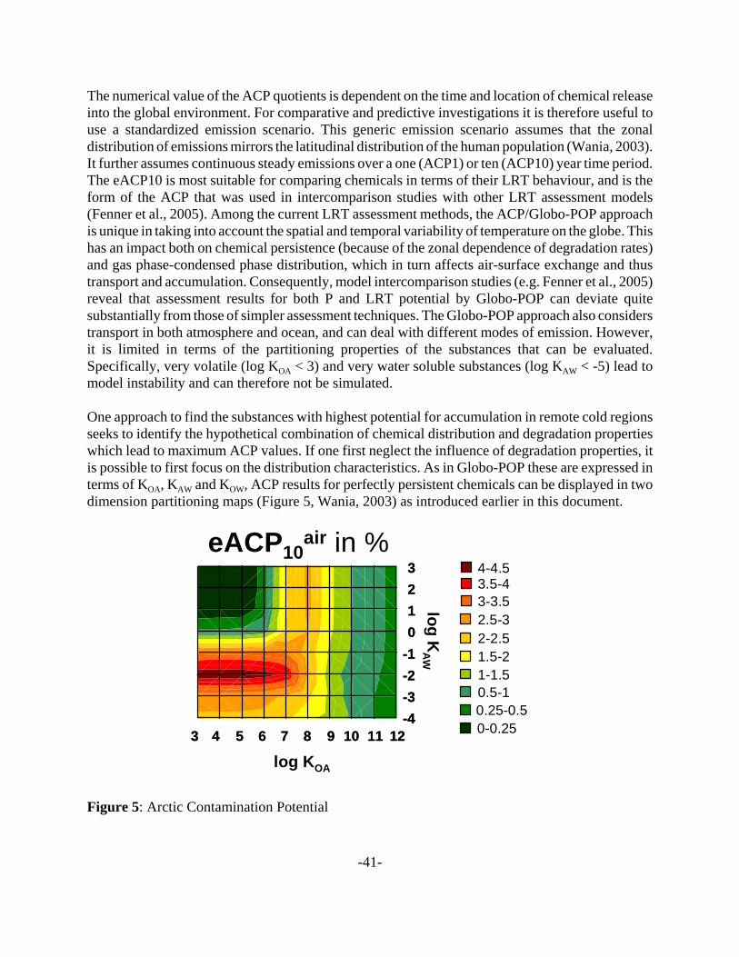
-41-

The numerical value of the ACP quotients is dependent on the time and location of chemical releaseinto the global environment. For comparative and predictive investigations it is therefore useful touse a standardized emission scenario. This generic emission scenario assumes that the zonaldistribution of emissions mirrors the latitudinal distribution of the human population (Wania, 2003).It further assumes continuous steady emissions over a one (ACP1) or ten (ACP10) year time period.The eACP10 is most suitable for comparing chemicals in terms of their LRT behaviour, and is theform of the ACP that was used in intercomparison studies with other LRT assessment models(Fenner et al., 2005). Among the current LRT assessment methods, the ACP/Globo-POP approachis unique in taking into account the spatial and temporal variability of temperature on the globe. Thishas an impact both on chemical persistence (because of the zonal dependence of degradation rates)and gas phase-condensed phase distribution, which in turn affects air-surface exchange and thustransport and accumulation. Consequently, model intercomparison studies (e.g. Fenner et al., 2005)reveal that assessment results for both P and LRT potential by Globo-POP can deviate quitesubstantially from those of simpler assessment techniques. The Globo-POP approach also considerstransport in both atmosphere and ocean, and can deal with different modes of emission. However,it is limited in terms of the partitioning properties of the substances that can be evaluated.Specifically, very volatile (log KOA < 3) and very water soluble substances (log KAW < -5) lead tomodel instability and can therefore not be simulated.

One approach to find the substances with highest potential for accumulation in remote cold regionsseeks to identify the hypothetical combination of chemical distribution and degradation propertieswhich lead to maximum ACP values. If one first neglect the influence of degradation properties, itis possible to first focus on the distribution characteristics. As in Globo-POP these are expressed interms of KOA, KAW and KOW, ACP results for perfectly persistent chemicals can be displayed in twodimension partitioning maps (Figure 5, Wania, 2003) as introduced earlier in this document.

Figure 5: Arctic Contamination Potential

4-4.53.5-43-3.52.5-32-2.51.5-21-1.50.5-10.25-0.50-0.25

eACP10air in %

3 5 6 7 8 9 10 121143 5 6 7 8 9 10 12114

log KOA

3210

-1-2-3-4

3210

-1-2-3-4

log KA

W

-42-

The ACP of a perfectly persistent organic chemical tends to be higher for two combinations ofpartitioning properties: relatively volatile (log KOA < 9) and water soluble (4 > log KAW > -0.5)substances and substances which are semi-volatile (6.5 < log KOA< 10) and relatively hydrophobic(log KAW > -3). Very volatile chemicals with log KOA < 6.5 and log KAW > -0.5 remain in theatmosphere even under Arctic temperature conditions, whereas very involatile chemical with a logKOA > 10 are efficiently and irreversibly deposited with atmospheric particles before reaching theArctic (Wania, 2003).

As a result, the ACP can be rapidly estimated for any persistent chemical from its location on thechemical space diagram. It is believed that such diagrams can be used in other contexts in whichpartitioning properties are important.

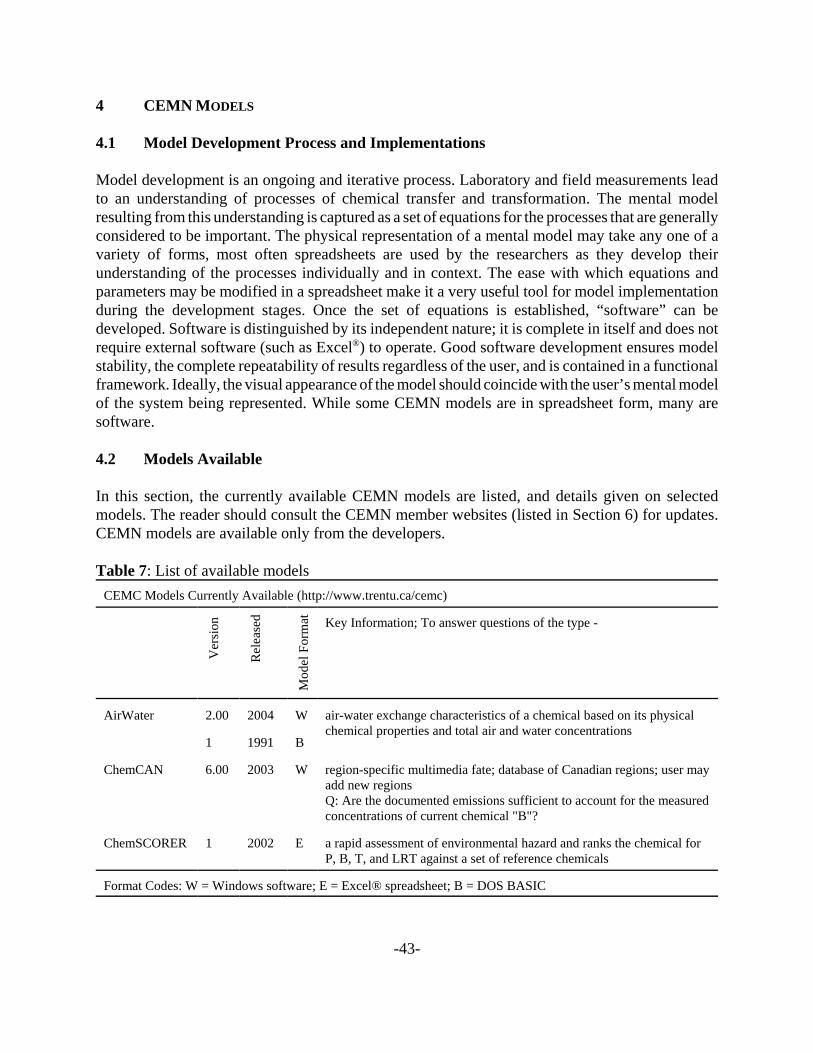
-43-

4 CEMN MODELS

4.1 Model Development Process and Implementations

Model development is an ongoing and iterative process. Laboratory and field measurements leadto an understanding of processes of chemical transfer and transformation. The mental modelresulting from this understanding is captured as a set of equations for the processes that are generallyconsidered to be important. The physical representation of a mental model may take any one of avariety of forms, most often spreadsheets are used by the researchers as they develop theirunderstanding of the processes individually and in context. The ease with which equations andparameters may be modified in a spreadsheet make it a very useful tool for model implementationduring the development stages. Once the set of equations is established, “software” can bedeveloped. Software is distinguished by its independent nature; it is complete in itself and does notrequire external software (such as Excel®) to operate. Good software development ensures modelstability, the complete repeatability of results regardless of the user, and is contained in a functionalframework. Ideally, the visual appearance of the model should coincide with the user’s mental modelof the system being represented. While some CEMN models are in spreadsheet form, many aresoftware.

4.2 Models Available

In this section, the currently available CEMN models are listed, and details given on selectedmodels. The reader should consult the CEMN member websites (listed in Section 6) for updates.CEMN models are available only from the developers.

Table 7: List of available modelsCEMC Models Currently Available (http://www.trentu.ca/cemc)

Ver

sion

Rel

ease

d

Mod

el F

orm

at Key Information; To answer questions of the type -

AirWater 2.00 2004 W air-water exchange characteristics of a chemical based on its physicalchemical properties and total air and water concentrations

1 1991 B

ChemCAN 6.00 2003 W region-specific multimedia fate; database of Canadian regions; user mayadd new regionsQ: Are the documented emissions sufficient to account for the measuredconcentrations of current chemical "B"?

ChemSCORER 1 2002 E a rapid assessment of environmental hazard and ranks the chemical forP, B, T, and LRT against a set of reference chemicals

Format Codes: W = Windows software; E = Excel® spreadsheet; B = DOS BASIC

-44-

CEMC Models Currently Available (http://www.trentu.ca/cemc) - continued

Ver

sion

Rel

ease

d

Mod

el F

orm


EQC 2.02 2003 W evaluative multimedia fate; combines LI, LII and LIII calculations;facilitates a progressive understanding of a chemical's fate in a standardenvironmentQ: In general terms, how will the (new) chemical "A" behave in theenvironment?

Fish 2 2004 W single organism model treats the steady-state uptake and release of anorganic chemical by a fish

1 1991 B

Foodweb 1 1991 B contaminant flux through an aquatic foodweb

Generic 1 1991 B early version of EQC

Level I 3.00 2004 W multimedia partitioning

Level II 2.17 1999 W multimedia partitioning and fate, assuming equilibrium

Level III 2.70 2004 W multimedia partitioning and fate, assuming steady-state

Level I, II, III 1 1991 B earlier version of the above set of software

QWASI 2.80 2002 W Focus on aquatic environment (lake); aquatic fate, assuming singlewell-mixed waterbody and steady-stateQ: What is the concentration of chemical "C" in Dexs Lake?1 1991 B

RateCon 1 1991 B designed to predict the fate and recovery times of contaminants in theGreat Lakes; similar to QWASI but not using the fugacity concept

Sediment 2 2004 W calculates the water-sediment exchange characteristics of a chemicalbased on its physical chemical properties and total water and sedimentconcentrations

Soil 2 2004 W very simple assessment of the relative potential for degrading reaction,evaporation, and leaching of a pesticide applied to a surface soil

1 1991 B

STP 2.1 2004 W engineered system sewage treatment plantQ: What are the key removal processes for chemical "D" in a definedSTP?

1 1991 B

TaPL3 3.00 2003 W Transport and persistence estimationsP and LRT in multimedia environment, assuming steady-stateQ: How do the persistence and LRT of the chemicals in this setcompare?


-45-

CEMC Models Currently Available (http://www.trentu.ca/cemc) - continued

Ver

sion

Rel

ease

d

Mod

el F

orm


PBPK 1 2003 E Physiologically-Based Pharmacokinetic model, describes disposition ofcontaminants within the human body

Multi-species 1 2003 E fate of a chemical with up to 3 other chemical species (reversible orirreversible conversion)

High resolutionMulti-species

4.1 2003 E multi-species chemical, more highly resolved and segmentedenvironment


Wania Models Currently Available (http://www.utsc.utoronto.ca/~wania)All are Windows software in format.

Version Released Key Information

LSER-Level III 1 2003 calculates Z-values using linear solvation energy relationships(LSERs) rather than partitioning properties such as watersolubility, vapour pressure, KOW

Cozmo-POP 1 2000 dynamic multimedia fate and transport model describes the long-term fate of POPs in a coastal environmentor the drainage basin of a large lake

Cozmo-POP 2 2 2005 increased and flexible spatial resolution of the aquaticenvironment and the improved description of the sedimentsand the processes associated with sediments

Globo-POP 1 1995 glo

ERTG Models Currently Available (http://www.rem.sfu.ca/toxicology/)All are Excel® spreadsheet format.

Version Released Key Information

BAF-AqWeb-Site 1 1993 site-specific aquatic food web bioaccumulation

BAF-AqWeb-Site 2 2004 site-specific aquatic food web bioaccumulation

BAF-AqWeb-QSAR 1 2003 generic aquatic food web bioaccumulation

Cautionary Note: The entries in the chemical databases included with most software models listed herecan be modified therefore it is the responsibility of the user to ensure that the values arecorrect by consulting a reference such as that of Mackay et al. (2000).

-46-

4.2.1 Choosing a model

When choosing the model for a particular task the parameters of the task, the expectations, and theacceptability of assumptions must be considered.

For general assessments not specific to a particular location, models such as EQC are helpful forgaining a general impression of the likely behaviour of a substance. These models are most usefulfor chemicals that are multimedia in nature, i.e., realistically present in all environmental media.

In chemical assessments, for single-medium substances, i.e., substances with a realistic presence inonly one environmental medium, a model with a detailed description of processes in that mediumshould be used to understand the likely behaviour of the substance. For example, a very volatilesubstance with a low KOA and a high KAW is likely to be present only in air. For such a substance adispersion model will provide an estimate of concentrations in the air at various distances from thesource. For such a substance, a multimedia model such as EQC which gives an averageconcentration in air over a large area, would require more input information without providing thespatial detail available from the dispersion model.

For a discharge to a river or lake, a water quality model such as QWASI gives an estimate ofaverage concentrations in the water and sediment. Again, this is more useful in this case than amodel such as EQC. If the substance being discharged is very volatile, QWASI gives an estimateof volatilization but assumes a fixed (user-specified) concentration in the air. To better determinethe concentration in the air, a model which calculates this value must be used.

Some guidance is provided with each model as to the original intended uses of the model. Using amodel for a purpose other than that for which it was designed may cause it to give mis-leadingresults and should be avoided. A careful examination of the equations in a model can assist indetermining the appropriateness of a model for a purpose.

Some models such as Level III, EQC, TaPL3, and ChemCAN contain many of the same equations;they all contain Level III calculations. The differences are the result of a progressive increase in ourunderstanding of environmental processes, the intended uses of the model, and the needs of theproject(s) underway during the development of the model. The Level III model is a generalimplementation of the Level III calculations and can be made to mimic many of the results from theother three. However, it is easier to use ChemCAN, for example, when modelling chemical fate inSouthern Quebec.

Figure 6 illustrates a suggested modelling process and decision tree that the user may find helpful.

Yes

NoThe substanceEmitted from a single point source?

The results

Area < 10000 km2 ?

Biotic (flora or fauna)?

Aquatic? Location-specific?

NoYes

No

YesNo

The environment

The modelEQC, the Level I, II, III set, TaPL3

! General features ofchemical behaviour

! Suitable for rankingchemicals

The environment

Yes

The model

Dispersion model (local-scale)

! Local fate and exposure! Concentration dilution

The environment

Single organism?

Yes

No

Yes

No

The modelPBPK, “Fish”, or others?

The results

! Chemical fate withinthe organism

! BCF, BAF! Tissue concentrations

The modelFoodWeb, EcoWeb, others?

The results

! Chemical fate withinthe food web

! Concentrations attrophic levels

! BCF, BAF, BMF

The environmentThe environment

The model

QWASI model

! Fatein a lakeor riversystem

! Single concentrationfor water column ofwhole system

The results

The results

The model

ChemCAN

! Ambientconcentrations in theregion modelled

! Suitable for comparingto monitoring data

The results

The modelLocal-scale steady-state Model?

! Expectations?

The results

Steady-state achieved?

Yes

NoThe environment

Yes

Area < 10000 km2 ?

The environment

The model

Dispersion model (local-scale)

! Local fate and exposure! Concentration dilution

The results

Yes The modelLevel IV, GloboPOP, others?

! Concentrations overtime

! Suitable for comparingto monitoring datatrends

The results

The substanceLikely to be present in >1environmental medium?

No

Single-medium model is neededThe model

The substance:data collection

Physical chemical propertiesLevel I (using a standardenvironment) or EQC (Level I)

The model Level II (using a standardenvironment) or EQC (Level II)

The modelThe substance:data collection

Degradation half-lives(in the absence of data,for media in which it isnot realisticallypresent, an infinitehalf-life may beassumed)

Yes

The results! Relative amounts in

each medium, i.e.,partitioning amongenvironmental media

! 1st estimate ofbioconcentration

The substance

The results! 1st estimate of

persistence! Relative importance of

each degradationprocess

Likely to be persistent,or bioaccumulative?

Modelling is likely unnecessary.Proceed as for a persistent orbioacummulative substance ifdesired.

A

Modelling Process and Decision Tree

No

YesLevel III (using a standardenvironment) or EQC (Level III)

The modelThe substance:data collectionMode-of-entry

The results! Improved estimate of

persistence! LRT potential may be

calculated! Relative rates of intermedia

transfer processes, lossprocesses

The substance:data collection

Emission data: rates,source types

A

-48-

4.3 Details on Selected CEMN Models

4.3.1 Level I Model (Version 3.00)

Model OverviewA Level I simulation is of the equilibrium distribution of a fixed quantity of conserved (ie.non-reacting) chemical, in a closed environment at equilibrium, with no degrading reactions, noadvective processes, and no intermedia transport processes (e.g. no wet deposition, orsedimentation). The medium receiving the emission is unimportant because the chemical is assumedto become instantaneously distributed to an equilibrium condition.

Physical-chemical properties are used to quantify a chemical’s behaviour in an evaluativeenvironment. Three types of chemicals are treated in this model: chemicals that partition into allmedia (Type 1- excluding ionizing chemicals), involatile chemicals (Type 2), and chemicals withzero, or near-zero, solubility (Type 3). Details on chemical Types are given in Section3.5.1.

Level I assumes a simple, evaluative, closed environment with user-defined volumes and densitiesfor the following seven homogeneous environmental media (or compartments): air, water, soil,sediment, suspended particles, fish and aerosols.

If one of the environmental media, soil for example, is removed by reducing its volume to zero, thenthe chemical will partition among the remaining media. That is, the amount of chemical, expressedas a percentage of the total dose, will increase in each of air, water, sediment, suspended particles,fish and aerosols. The total amount of chemical remains the same. A feature of the model is thateven with a zero volume of a medium, soil in this example, a concentration is still calculated for thezero volume medium. This is the concentration the medium would have if it were present. This ispossible since equilibrium is assumed and thus the fugacity of the medium is known and theconcentration is the product of the fugacity, f, and the fugacity capacity, Z, of the medium which isindependent of the presence of the medium.

The required model input data and a list of results are given in Table 8.

A complete description of the Level I calculations is given in the textbook on fugacity models byMackay (2001).

Intended UsesThis model is useful for establishing the general features of a new or existing chemical’s behaviour.A Level I calculation gives the general impression of the likely media into which a chemical willtend to partition and an indication of relative concentrations in each medium and between sub-compartments in each medium. For example, a Level I calculation can be used to investigate thephase distribution of organic chemicals in the atmosphere at equilibrium, that is the relativedistribution between gas phase, atmospheric particles, and water droplets. The results can again bedisplayed in partitioning space maps as discussed in Section 3.5.1 Similarly, Level I calculations canbe used to investigate the equilibrium phase distribution within a soil (i.e. between the soil organic

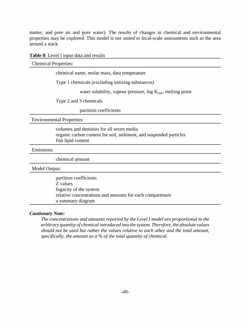
-49-

matter, and pore air and pore water). The results of changes in chemical and environmentalproperties may be explored. This model is not suited to local-scale assessments such as the areaaround a stack.

Table 8: Level I input data and results

Chemical Properties:

chemical name, molar mass, data temperature

Type 1 chemicals (excluding ionizing substances)

water solubility, vapour pressure, log KOW, melting point

Type 2 and 3 chemicals

partition coefficients

Environmental Properties:

volumes and densities for all seven mediaorganic carbon content for soil, sediment, and suspended particlesfish lipid content

Emissions:

chemical amount

Model Output:

partition coefficientsZ values fugacity of the system relative concentrations and amounts for each compartment a summary diagram

Cautionary Note: The concentrations and amounts reported by the Level I model are proportional to thearbitrary quantity of chemical introduced into the system. Therefore, the absolute valuesshould not be used but rather the values relative to each other and the total amount,specifically, the amount as a % of the total quantity of chemical.

-50-

4.3.2 Level II Model (Version 2.17)

Model OverviewA Level II simulation describes a situation in which a chemical is continuously discharged at aconstant rate and achieves a steady-state and equilibrium condition at which the input and outputrates are equal. Degrading reactions and advective processes are the loss or output processes treated.Intermedia transport processes (eg. no wet deposition, or sedimentation) are not quantified. Themedium receiving the emission is unimportant because the chemical is assumed to becomeinstantaneously distributed to an equilibrium condition.

Physical-chemical properties are used to quantify a chemical’s behaviour in an evaluativeenvironment. Three types of chemicals are treated in this model: chemicals that partition into allmedia (Type 1- excluding ionizing chemicals), involatile chemicals (Type 2), and chemicals withzero, or near-zero, solubility (Type 3). Level II assumes a simple, evaluative environment withuser-defined volumes and densities for the following homogeneous environmental media (orcompartments): air, water, soil, sediment, suspended particles, fish and aerosols. “Fish” is a genericaquatic biotic organism.

Three residence times are calculated, an overall value, TO, and individual residence time attributableto reaction only, TR, and advection only, TA. Note that 1/TO equals the sum of 1/TR and 1/TA. Therelative contribution of advection and reaction to the total removal of chemical depends strongly onthe size of the system as noted in Section 3.5.2. However, consideration of advection and reactionrates allows for the calculation of chemical persistence. It provides a first estimate of overallenvironmental persistence, which is a critical property of the chemical. It also shows which lossprocesses are likely to be most important. A fast reaction or short half-life may not be significantif relatively little of the chemical is subject to this reaction by virtue of its partitioning. The potentialfor the chemical to be subject to long-range atmospheric transport is also indicated by the magnitudeof the air advection loss. While this version of the Level II model does not explicitly calculate LRTit can be calculated manually as the product of an assumed wind speed (km/h), the overall residencetime of the chemical (h), and the ratio of the amount in air to the total amount in the system as wasdone for the collaboration with Fenner et al (2005) . The global chemical persistence is bestindicated by the reaction residence time, whereas the local persistence is indicated by the overallresidence time.

Note that in this version, reaction half-lives are requested for all seven media. In previous versionsreactions in only four media were treated. In the absence of data, the half-lives for suspendedparticles and fish can be assumed to be equal to that of the water, and that of aerosols can beassumed to be equal to that of air.

The advective residence time selected for air applies to aerosols and the residence time for waterapplies to suspended sediment and fish. The advective residence time of aerosols, suspendedparticles and fish cannot be specified independently of the air and water residence times. Theseresidence times are the time that the air, for example, spends in the modelled system. It is relatedto the prevailing wind direction and the distance across the region in that direction. Since only the

-51-

area of the region is specified in the model, the residence time is not automatically adjusted by thesoftware when the area is changed by the user. When the total area of the region is reduced and theresidence time is retained, the flow rate of the air (volume/residence time) is reduced. The D valuefor this loss process (flow rate × Z value) is also reduced. The fugacities and concentrations allincrease. Since the rates of loss are the product of the fugacity and the D value the increase in thefugacity is matched by the decrease in D value, no change is seen in the rates of loss. Similarlyamounts of chemical, being the product of concentration and volume, are unchanged.

Cautionary Note: These advective residence times do not represent dilution. The air and water are eachconsidered to be well-mixed boxes and thus there is no dilution effect with distance.Advection is a removal process, physically moving the contaminated air or water intothe adjoining region.

A Level II calculation is more realistic than a Level I calculation but requires additional information.The additional model input data and a list of results are given in Table 9.

A complete description of the Level II calculations is given in the textbook on fugacity models byMackay (2001).

Intended UsesThis model is useful for establishing the general features of a new or existing chemical's behaviour.A Level II calculation gives an indication of the likely media into which a chemical will tend topartition and an indication of relative concentrations in each medium. The distribution betweenmedia is the same as in Level I. The results of changes in chemical and environmental propertiesmay be explored. This model is not suited to local-scale assessments such as the area around a stack.

Table 9: Additional input data required by Level II and the additional results generated.


reaction half-life estimates for all seven media


advective flow residence time for air (including aerosols)advective flow residence time for water (including suspended particles, fish) advective flow residence time for sediment burial

Emissions:

chemical input rate inflowing concentrations in air and water

-52-

Model Output:

D values reaction and advection loss rates chemical residence times (overall, reaction, and advection)

Cautionary Note: As for Level I, the concentrations and amounts reported by the Level II model areproportional to the arbitrary emission rate. Therefore, the absolute values should notbe used but rather the values relative to each other and the total amount. Specifically,of interest is the amount as a % of the total quantity of chemical and the relativeimportance of the loss processes.

4.3.3 Level III Model (Version 2.80)

Model OverviewA Level III simulation describes a situation which is one step more complex and realistic than theLevel II model. Like the Level II model, chemical is continuously discharged at a constant rate andachieves a steady state condition in which input and output rates are equal. The loss processes aredegrading reactions and advection. Unlike the Level II model, equilibrium between media is notassumed and, in general, each medium is at a different fugacity. A mass balance applies not only tothe system as a whole, but to each compartment. Rates of intermedia transport are calculated usingD values which contain information on mass transfer coefficients, areas, deposition and resuspensionrates, diffusion rates, and soil runoff rates. It is now essential to define inputs to each mediumseparately, whereas in Level II only the total input rate was requested. The additional model inputdata and a list of results are given in Table 8.

Mass balances are calculated for the four bulk media of air (gas + aerosol), water (solution +suspended particles + biota), soil, (solids + pore air + pore water), and sediment (solids + porewater). Equilibrium exists within, but not between media. For example, sediment solids and porewater are at equilibrium, but sediment is not necessarily at equilibrium with the overlying water.

Physical-chemical properties are used to quantify a chemical’s behaviour in an evaluativeenvironment. Three types of chemicals are treated in this model: chemicals that partition into allmedia (Type 1- excluding ionizing chemicals), involatile chemicals (Type 2), and chemicals withzero, or near-zero, solubility (Type 3). The model can not treat ionizing or speciating substances.The Level III model assumes a simple, evaluative environment with user-defined volumes anddensities for the following homogeneous environmental media (or compartments): air, water, soil,sediment, suspended particles, fish and aerosols. “Fish” is a generic aquatic biotic organism.

A complete description of the Level III calculations is given in the textbook on fugacity models byMackay (2001).

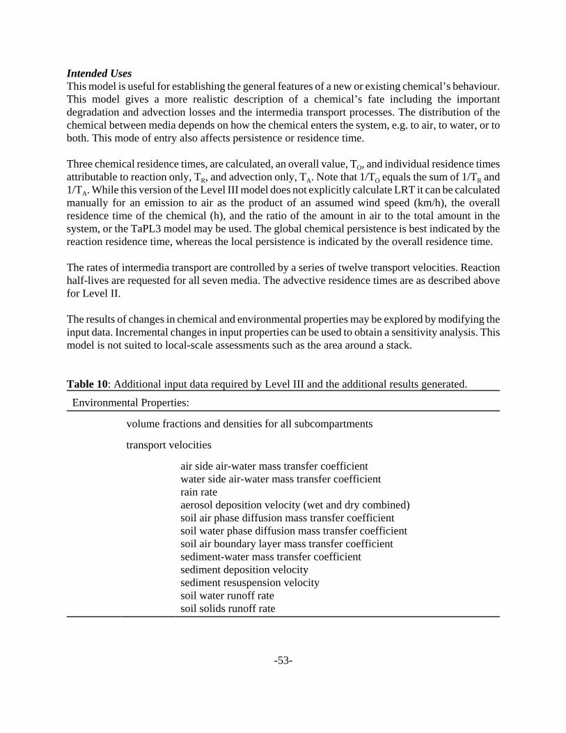
-53-

Intended UsesThis model is useful for establishing the general features of a new or existing chemical’s behaviour.This model gives a more realistic description of a chemical’s fate including the importantdegradation and advection losses and the intermedia transport processes. The distribution of thechemical between media depends on how the chemical enters the system, e.g. to air, to water, or toboth. This mode of entry also affects persistence or residence time.

Three chemical residence times, are calculated, an overall value, TO, and individual residence timesattributable to reaction only, TR, and advection only, TA. Note that 1/TO equals the sum of 1/TR and1/TA. While this version of the Level III model does not explicitly calculate LRT it can be calculatedmanually for an emission to air as the product of an assumed wind speed (km/h), the overallresidence time of the chemical (h), and the ratio of the amount in air to the total amount in thesystem, or the TaPL3 model may be used. The global chemical persistence is best indicated by thereaction residence time, whereas the local persistence is indicated by the overall residence time.

The rates of intermedia transport are controlled by a series of twelve transport velocities. Reactionhalf-lives are requested for all seven media. The advective residence times are as described abovefor Level II.

The results of changes in chemical and environmental properties may be explored by modifying theinput data. Incremental changes in input properties can be used to obtain a sensitivity analysis. Thismodel is not suited to local-scale assessments such as the area around a stack.

Table 10: Additional input data required by Level III and the additional results generated.


volume fractions and densities for all subcompartments

transport velocities

air side air-water mass transfer coefficient water side air-water mass transfer coefficient rain rate aerosol deposition velocity (wet and dry combined) soil air phase diffusion mass transfer coefficient soil water phase diffusion mass transfer coefficient soil air boundary layer mass transfer coefficient sediment-water mass transfer coefficient sediment deposition velocity sediment resuspension velocity soil water runoff rate soil solids runoff rate

-54-

Emissions:

chemical input rates for each bulk medium or compartment inflow concentrations in air and water

Model Output:

fugacity of each medium intermedia transport rates and D values charts of key results

4.3.4 LSER-Level III

Model OverviewBreivik and Wania (2003) have developed a steady-state model, which differs with respect to theestimation of phase partitioning. Other Level III-type models require the input of physical chemicalproperties such as water solubility, vapour pressure, melting point, and KOW. These input parametersare used to estimate such partition coefficients as KAW, KOC, and KQA. Z-values for all environmentalmedia are then derived from these partition coefficients.

The LSER-Level III model alternatively allows for the calculation of Z-values using linear solvationenergy relationships (LSERs). These commonly take the form:

(35)

or

(36)log logSP c rR s a b l LH H H

= + + + ∑ + ∑ +2162 2 2π α β

where SP refers to the phase partition property of interest. In general, equation (35) is commonlyapplied to processes involving two condensed phases, while equation (36) is typically applied forthe distribution between the gas-phase and a condensed phase. These equations consist of productterms representing the properties of the chemical (solute descriptors) and the environmental media(system constants) - the latter as identified by lower-case Latin characters. Each product term thusrepresents the contribution of a specific intermolecular interaction to the overall partition propertyof interest.

The chemically specific solute descriptors in LSERs are the excess molar refraction (R2 in cm3/10),a dipolarity/polarizability term ( ), the effective or overall hydrogen-bond acidity andπ2

H

hydrogen-bond basicity ( and respectively), as well as an indicator of solute size.α2H∑ β2

H∑LSERs of the type equation (35) use McGowan's characteristic volume VX (in cm3 mol-1 / 100), while

log SP c rR s a b vVH H H

X= + + + ∑ + ∑ +22 2 2π α β

-55-

those of type equation (36) include the distribution constant for the chemical between the gas phaseand n-hexadecane at 298 K (log L16). The coefficients (c, r, s, a, b, v and l) or system constants inequations 1 and 2 are defined by their complementary interactions with the solute descriptors. Ther constant determines the difference in capacity of the two phases considered with respect to theirn- or -electron interaction with the chemical (solute). The s constant is a measure of the differencein capacity of the two phases to participate in dipole-dipole and dipole-induced dipole interactionswith the chemical. The a and b constant express the difference between the two phases with respectto their hydrogen-bond acidity and hydrogen-bond basicity, respectively. Finally, the l and mconstants are measures of the relative ease of the chemical to form a cavity in the two phasesconsidered (i.e. the so-called cavity term).

In summary, whereas other Level III-type models require the input of a chemical’s vapour pressureand water solubility, and KOW, the LSER-Level III model requires the input of a chemical’s LSERsolute descriptors. Specifically, the use of the LSER-Level III model should be considered when:

- the validity of relationships in other Level III-type models is in doubt. This appliesparticularly to organic substances with polar functional groups that interact by hydrogen-bonds withvarious environmental phases (Breivik and Wania, 2003).

- if reliable experimental values of the “classical” physical-chemical partitioning properties(P, SW, KOW, KAW, KOA) are not available. The LSER solute descriptors, if not available fromtabulations, can be estimated from molecular structure using quantitative structure propertyrelationships (QSPR) (Platts et al., 1999).

4.3.5 EQC Model (Version 2.02)

Model OverviewThe EQC, or EQuilibrium Criterion, model uses chemical-physical properties to quantify achemical's behaviour in an evaluative environment. This model combines the Level I, II and IIIcalculations in a single model and treats the same three chemical Types but with a fixed environmentto facilitate chemical-to-chemical comparison.

A more detailed description of the model is given in the three paper set by Mackay et al (1996a-c):

All of the chemical data required for a Level III calculation are required by EQC with the exceptionthat the degradation half-lives for aerosols, suspended particles and fish are assumed to be equal tothose for air and water respectively. Degradation data for these media are often unavailable makingthis a convenient model simplification.

The environmental parameters in this model may not be changed by the user. This focusses attentionon chemical-to-chemical differences. In this version of the EQC model, unlike previous versions,all environmental properties are displayed and recorded with the model output. Only for the LevelIII calculations are the soil and sediment compartments sub-divided into solid, air, and water

-56-

fractions. The depth of the soil and sediment compartments for Level I and II calculations arereduced to simulate only the solid fraction. Thus the concentrations for these compartments shouldbe considered as dry weight concentrations when comparing to Level III results.

A set amount of chemical and a set discharge rate are used in the Level I and II calculations in EQC.The user may specify the proportional emissions to air, water, and soil for the Level III calculation.

Intended UsesThis model is useful for establishing the general features of a new or existing chemical's behaviour,ie. the media into which the chemical will tend to partition, the primary loss mechanisms, and itstendency for intermedia transport. The result of various emission scenarios can be explored. Thismodel is not suited to local-scale assessments such as the area around a stack.

4.3.6 ChemCAN Model (Version 6.00)

Model OverviewThis far-field, Level III model contains a database of 24 regions of Canada. It estimates averageconcentrations in air, fresh surface water, fish, sediments, soils, vegetation, and marine near-shorewaters. It is intended to assist in human exposure assessment where a specific target population maybe identified. Designed for use in Canada, a database of 24 regions of Canada is included. Otherregions can be defined by the user and added to the database, however, areas should have a radiusof at least 300 km. For surface areas of a region it is not recommended going less than about 10000km2 (100x100 km) or larger than about 1000000 km (1000 x 1000 km). For investigations involvingsmaller areas, air dispersion will dominate and a plume model may be more appropriate. If the userhas data for the region of interest, this can be used in place of values in the database. Table 11 liststhe environmental properties required.

The regional divisions of Canada were based on the ecozones identified by Environment Canada andwith consideration of the distribution of population and industrial activity, political boundaries,drainage basins, and climate to give areas of sufficiently homogeneous ecological conditions suchthat meaningful assessments of chemical fate can be conducted.

Cautionary Note: An "average" region is also included in the database. This should not be used for anychemical assessment. It is included to assist in any exploration of the range of resultspossible for different regions as was done by Webster et al (2004b). For a non-regionspecific evaluation, use the "EQC standard environment" included in the ChemCANdatabase with an emission proportional to the population density of southern Ontariocompared to Canada as a whole. The releases will be different in each region and thefate will be different. Using the "average" region and an "average" emission will givea result unrepresentative of any region of Canada to a degree dependent upon thechemical.

-57-

To estimate upwind concentrations, an air (or water) inflow concentration of perhaps 25% of theoutput concentration can be selected from a “clean air” run of the model, and the model re-run withthis estimate.

This model requires all of the same chemical property information as the Level III model, however,the user is given more options in entering the partitioning data for Type 1 chemicals. This is a matterof both convenience and allows a wider set of data to be mined for the best values. Any two of thethree partition coefficients, octanol-water (KOW), octanol-air (KOA), or air-water (KAW) are sufficient.This reflects the so-called three solubilities approach (Cole and Mackay 2000). If the user choosesto supply the air-water partition coefficient, it may be entered as the dimensionless partitioncoefficient KAW, Henry’s law constant, or the water solubility and vapour pressure. The temperaturedependence coefficients for the partition coefficients are also required for Type 1 chemicals. Thus,for Type 1 chemicals, the model is able to apply temperature corrections to the partitioningproperties. For Types 2 and 3 these corrections must be made manually by the user. In addition,partitioning parameters for aerosols are required based on Finizio et al (1997) relationships. Onlythe four primary degradation half-lives are required.

The temperature dependence coefficients and the constants for the partitioning to aerosols estimationmethods require data that may be difficult to obtain. Some “standard” values are provided, howeverthese are based on a very limited data set. It is best to use chemical-specific values if possible. Formore information, refer to the work of Beyer et al (2002) on temperature dependence and to thesource of the partitioning to aerosols correlation (Finizio et al 1997).

Table 12 lists the emission data requirements for and results from ChemCAN.

A more complete description of this model is given by Webster et al (2004b).

Intended UsesThe ChemCAN model is intended to provide regionally-specific estimates of chemicalconcentrations in the primary media. These can be compared to monitoring data and used to estimateexposure. This model is not suited to local-scale assessments such as the area around a stack.

-58-

Table 11: Environmental properties required to define a region in ChemCAN.

dimensions of the environment

total surface area % water cover by area length of coastline for maritime regions average air height average water depth average soil depth average sediment depthlength of coastlineaverage coastal water depthaverage coastal widthvolume fractions and densities for all subcompartments

temperature conditions (winter, summer or annual average) residence times for air, water, and coastal waterorganic carbon content (soil, sediment, suspended particles) as a mass fractionfish and vegetation lipid content as a mass fractiona fitted, solids-water partition coefficient to calculate the sorption attenuation factor

transport velocities

air side air-water mass transfer coefficient water side air-water mass transfer coefficientrain rateaerosol deposition (dry only)soil air phase diffusion mass transfer coefficient soil water phase diffusion mass transfer coefficient soil air boundary layer mass transfer coefficient sediment-water mass transfer coefficient sediment deposition sediment resuspension soil water runoff soil solids runoff sediment burial diffusion to higher altitudesleaching from soil

rain and snow scavenging ratios

-59-

Table 12: Emission data requirements for and results from ChemCAN.

Emissions:

chemical input rates for each bulk medium or compartmentinflow concentrations in air and water

Model Output:

partition coefficientsZ valuesfugacity of each mediumintermedia transport rates and D valuesreaction and advection D values and loss ratesresidence times (overall, reaction, and advection)concentrations and amounts for each mediuma summary diagram

4.3.7 CoZMo-POP

Model OverviewCoZMo-POP 2 is a generic and flexible Level IV, i.e., dynamic, or unsteady-state, model that canbe adapted to a variety of applications requiring dynamic approaches without the need to change thesource code (Wania et al., submitted).

Even though the CoZMo-POP 2 was specifically designed as a dynamic multimedia fate andtransport model for describing the long term fate of persistent organic pollutants (POPs) in a coastalenvironment or the drainage basin of a large lake, it is sufficently generic and flexible to allow itsuse in a variety of contexts. The modelled environment, consisting of up to 19 compartments,includes the forest, soils and fresh water bodies of the drainage basin, and a variable number ofsequentially arranged marine water units, representing estuarine, coastal, open and deep waterenvironments. Two sediment compartments in each water basin allow to account for the possibilityof the simultaneous occurrence of eroding and accumulating bottoms in a water basin. In order toallow the user flexibility in terms of the spatial resolution of the water body, it is possible to reducethe complexity of the aquatic system by eliminating all but one water and two sedimentcompartments. The model region could thus contain one (fresh water), two (fresh and estuarinewater), three (fresh, estuarine and coastal water), or five water compartments. Additionalsimplification can be achieved by eliminating specific compartments (e.g. the forests, or soils)through defining artificially low compartment dimensions. The user may thus achieve a great degreeof flexibility in terms of defining the environmental systems to be studied.

As the movement of organic chemicals in the environment is closely associated with the movementof air, water and organic matter, the model constructs complete mass budgets for air, water andparticulate organic carbon (POC) between the model compartments from the environmental

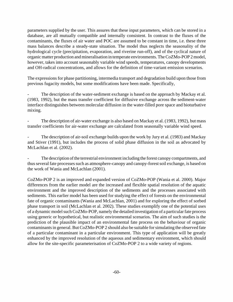
-60-

parameters supplied by the user. This assures that these input parameters, which can be stored in adatabase, are all mutually compatible and internally consistent. In contrast to the fluxes of thecontaminants, the fluxes of air water and POC are assumed to be constant in time, i.e. these threemass balances describe a steady-state situation. The model thus neglects the seasonality of thehydrological cycle (precipitation, evaporation, and riverine run-off), and of the cyclical nature oforganic matter production and mineralisation in temperate environments. The CoZMo-POP 2 model,however, takes into account seasonably variable wind speeds, temperatures, canopy developmentsand OH-radical concentrations, and allows for the definition of time-variant emission scenarios.

The expressions for phase partitioning, intermedia transport and degradation build upon those fromprevious fugacity models, but some modifications have been made. Specifically,

- The description of the water-sediment exchange is based on the approach by Mackay et al.(1983, 1992), but the mass transfer coefficient for diffusive exchange across the sediment-waterinterface distinguishes between molecular diffusion in the water-filled pore space and bioturbativemixing.

- The description of air-water exchange is also based on Mackay et al. (1983, 1992), but masstransfer coefficients for air-water exchange are calculated from seasonally variable wind speed.

- The description of air-soil exchange builds upon the work by Jury et al. (1983) and Mackayand Stiver (1991), but includes the process of solid phase diffusion in the soil as advocated byMcLachlan et al. (2002).

- The description of the terrestrial environment including the forest canopy compartments, andthus several fate processes such as atmosphere-canopy and canopy-forest soil exchange, is based onthe work of Wania and McLachlan (2001).

CoZMo-POP 2 is an improved and expanded version of CoZMo-POP (Wania et al. 2000). Majordifferences from the earlier model are the increased and flexible spatial resolution of the aquaticenvironment and the improved description of the sediments and the processes associated withsediments. This earlier model has been used for studying the effect of forests on the environmentalfate of organic contaminants (Wania and McLachlan, 2001) and for exploring the effect of sorbedphase transport in soil (McLachlan et al. 2002). These studies exemplify one of the potential usesof a dynamic model such CoZMo-POP, namely the detailed investigation of a particular fate processusing generic or hypothetical, but realistic environmental scenarios. The aim of such studies is theprediction of the plausible impact of an environmental fate process on the behaviour of organiccontaminants in general. But CoZMo-POP 2 should also be suitable for simulating the observed fateof a particular contaminant in a particular environment. This type of application will be greatlyenhanced by the improved resolution of the aqueous and sedimentary environment, which shouldallow for the site-specific parameterisation of CoZMo-POP 2 to a wide variety of regions.

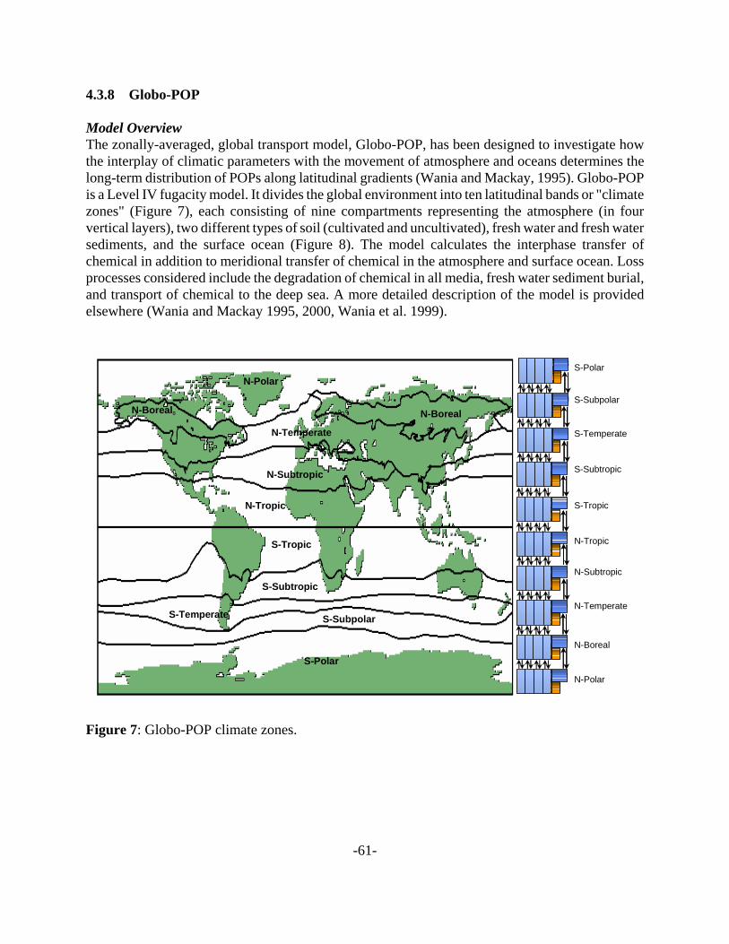
-61-

4.3.8 Globo-POP

Model OverviewThe zonally-averaged, global transport model, Globo-POP, has been designed to investigate howthe interplay of climatic parameters with the movement of atmosphere and oceans determines thelong-term distribution of POPs along latitudinal gradients (Wania and Mackay, 1995). Globo-POPis a Level IV fugacity model. It divides the global environment into ten latitudinal bands or "climatezones" (Figure 7), each consisting of nine compartments representing the atmosphere (in fourvertical layers), two different types of soil (cultivated and uncultivated), fresh water and fresh watersediments, and the surface ocean (Figure 8). The model calculates the interphase transfer ofchemical in addition to meridional transfer of chemical in the atmosphere and surface ocean. Lossprocesses considered include the degradation of chemical in all media, fresh water sediment burial,and transport of chemical to the deep sea. A more detailed description of the model is providedelsewhere (Wania and Mackay 1995, 2000, Wania et al. 1999).

Figure 7: Globo-POP climate zones.

N-Polar

N-Boreal

N-Temperate

N-Subtropic

N-Tropic

S-Subpolar

S-Temperate

S-Subtropic

S-Tropic

S-PolarN-Polar

N-Boreal

N-Temperate

N-Subtropic

N-Tropic

S-Tropic

S-Subtropic

S-Temperate S-Subpolar

S-Polar

N-Boreal

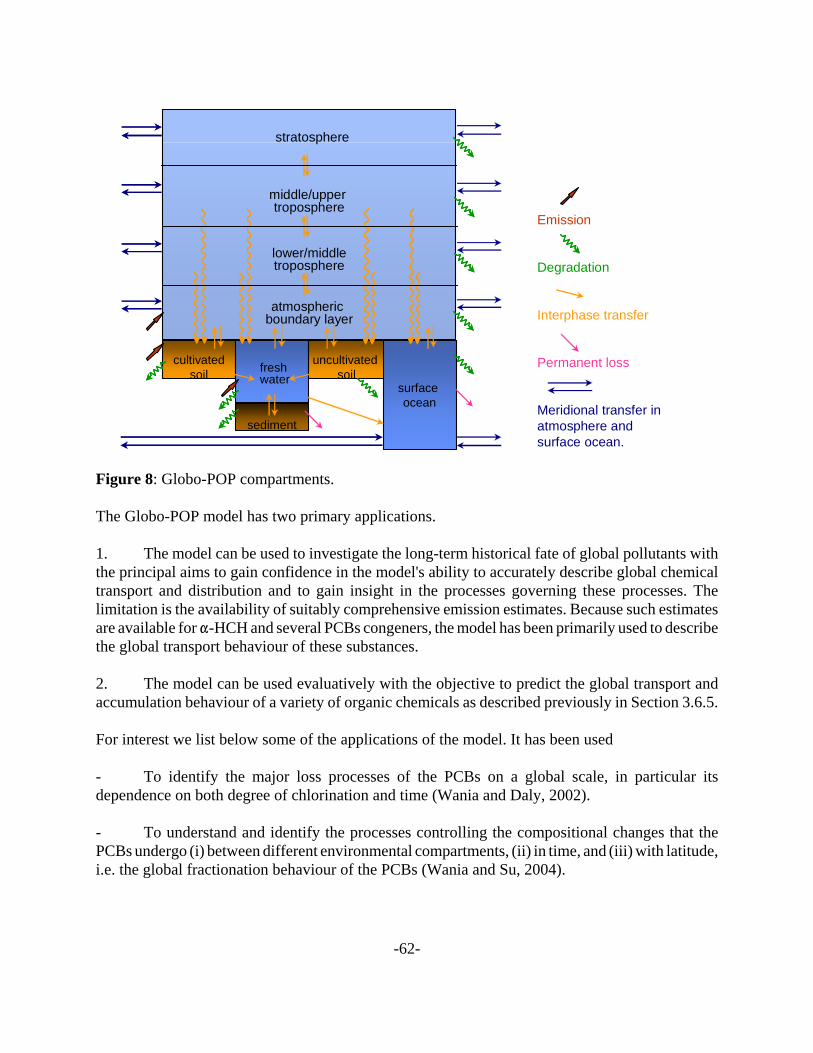
-62-

Figure 8: Globo-POP compartments.

The Globo-POP model has two primary applications.

1. The model can be used to investigate the long-term historical fate of global pollutants withthe principal aims to gain confidence in the model's ability to accurately describe global chemicaltransport and distribution and to gain insight in the processes governing these processes. Thelimitation is the availability of suitably comprehensive emission estimates. Because such estimatesare available for "-HCH and several PCBs congeners, the model has been primarily used to describethe global transport behaviour of these substances.

2. The model can be used evaluatively with the objective to predict the global transport andaccumulation behaviour of a variety of organic chemicals as described previously in Section 3.6.5.

For interest we list below some of the applications of the model. It has been used

- To identify the major loss processes of the PCBs on a global scale, in particular itsdependence on both degree of chlorination and time (Wania and Daly, 2002).

- To understand and identify the processes controlling the compositional changes that thePCBs undergo (i) between different environmental compartments, (ii) in time, and (iii) with latitude,i.e. the global fractionation behaviour of the PCBs (Wania and Su, 2004).

cultivatedsoil

uncultivated soil

surface ocean

sediment

stratosphere

middle/upper troposphere

lower/middletroposphere

atmospheric boundary layer

freshwater

Emission

Degradation

Interphase transfer

Permanent loss

Meridional transfer in atmosphere and surface ocean.

-63-

- To understand the processes that control, and to further seek to predict, the rate of declineof PCB air concentrations prior to, and after, the end of primary emissions (Hung et al., submitted).

- To evaluate its performance with regard to reproducing the observed fate and distributionof "-HCH in the global environment (Wania et al., 1999, Lakaschus et al., 2001).

- To understand the global cold-trapping behaviour of "-HCH, and understand its major globaltransport pathways (Wania and Mackay, 1999).

4.3.9 TaPL3 Model (Version 3.00)

Model OverviewThe TaPL3 model uses a Level III simulation to evaluate a chemical’s potential for long-rangetransport (LRT) in a mobile medium, either air, or water, its environmental persistence, and theaverage number of hops a molecule will experience.

Two scenarios are modelled; an emission to air where air is the mobile medium, and emission towater where water is the mobile medium. There is no advective removal from the environment. Thestickiness of each stationary medium with respect to the mobile medium is calculated where“stickiness” is the ratio of the net intermedia transport flux to the mobile-to-stationary flux, i.e., thefraction of chemical transported to the stationary medium that remains there.

A more detailed description of the calculations for persistence and long-range transport in this modelis given in Beyer et al (2000), Webster et al (1998), and Webster et al (2003).

This model requires all of the same chemical property information as the Level III model. Inaddition, for Type 1 chemicals, TaPL3 corrects both partitioning properties and degradation ratesfor temperature, thus the enthalpies for KOW and KAW and the activation energies for the half-livesare required. For Types 2 and 3, temperature corrections must be done manually by the user. In thisversion of the model a vegetation compartment is included in the mass balance therefore adegradation half-life in vegetation is also required.

If the chemical data were collected at the same temperature as the modelled environment, theequation collapses such that the value of the enthalpy has no effect. Of course, this is simplistic sincethe environment is seldom at the temperature of the lab. There are two “default” sets of values forthe enthalpies based on categories of chemicals. As a first pass, broad generalization, the values -20: 55 which were assigned to the X - hypothetical chemical for KOW : KAW may be used. However,these values are based on a limited set of similar substances and so may be inappropriate. Forchemical-specific data refer to Beyer et al (2002) and for a discussion of the influence oftemperature on LRT refer to Beyer et al (2003) .

The environmental properties are as required by the Level III model except that wind and waterspeeds replace the advection residence times for air and water. Vegetation biomass, leaf area index,

-64-

leaf-air boundary layer mass transfer coefficient, and fraction of rain intercepted by vegetation arerequired for the vegetation calculations since equilibrium is not assumed here as it is in many LevelIII calculations.

This model assumes a single emission rate to air and to water and calculates chemical fate separatelyfor each case.

Cautionary Note: All media are considered to be well-mixed boxes and thus there is no dilution effect. Anyemission is considered to be instantaneously distributed within the receiving mediumof air or water.

In addition to the standard Level III-type results for each of emission to air and emission to water,TaPL3 also reports:

- overall environmental persistence (i.e., the residence time in the environment due onlytothe degradation of the chemical)- long-range transport potential

LA for emission to, and transport in air and LW for emission to, and transport in water

- stickiness - average number of hops (emission to air only)

While the persistence may be taken as the longevity of the substance, the potential for long-rangetransport should be used as a ranking only and not as an actual distance travelled. Any distanceexceeding 1000 km is considered evidence of potential for LRT.

Table 13: Qualitative interpretations of values for LA

LA Qualitative interpretation

< 500 relatively little long-range atmospheric transport is expected

500 to 1000 potential for significant continental-scale transport

1000 to 3000 some global-scale transport is likely

> 3000 high potential for global-scale long-range atmospheric transport

-65-

Table 14: Persistence and LRT potential in air calculated by TaPL3 for a small set of substances.

Substance Persistence, d LA, km

HCB 4000 8000

Chlorobenzene 10 3800

Biphenyl 3.6 1100

deca-PCB 3300 400

Aldrin 0.4 100

Intended UsesThis model is intended as an evaluative tool to be used in the detailed assessment and ranking ofchemicals for potential for long-range transport in a mobile medium, either air, or water, and forpersistence. It is expected that the model will be primarily used to compare chemicals, not toestablish absolute values. The Level III model should be used for more general applications. Thismodel is not suited to local-scale assessments such as the area around a stack.

4.3.10 QWASI Model (Version 2.80)

Model OverviewThe “Quantitative Water Air Sediment Interaction” or “QWASI” model describes the steady-state(i.e., Level III) behaviour of an organic chemical in a lake subject to chemical inputs by directdischarge, inflow in rivers, and deposition from the atmosphere. Chemical is removed from the lakeby evaporation, irreversible reaction in the water and sediment, outflow in the water, and sedimentburial. The mass balance equations for the well-mixed water column and the well-mixed layer ofsurficial sediment also include sediment-water exchange by diffusion, deposition, and resuspension.

In contrast with, for example, the Level III model described in section 4.3.3, this Level III treatmentof an air-water-sediment system has a simpler treatment of air as a potential source of chemical tothe lake system. The air is assumed to maintain a constant concentration. No losses throughdegradation or advection in air are considered. The absence of any terrestrial compartment removesthe need for any soil parameters. Thus only relevant data are required by the QWASI model, andattention is focussed on chemical behaviour in the lake system.

The model, as supplied, treats PCBs in Lake Ontario.

The required input data are given in Table 15.

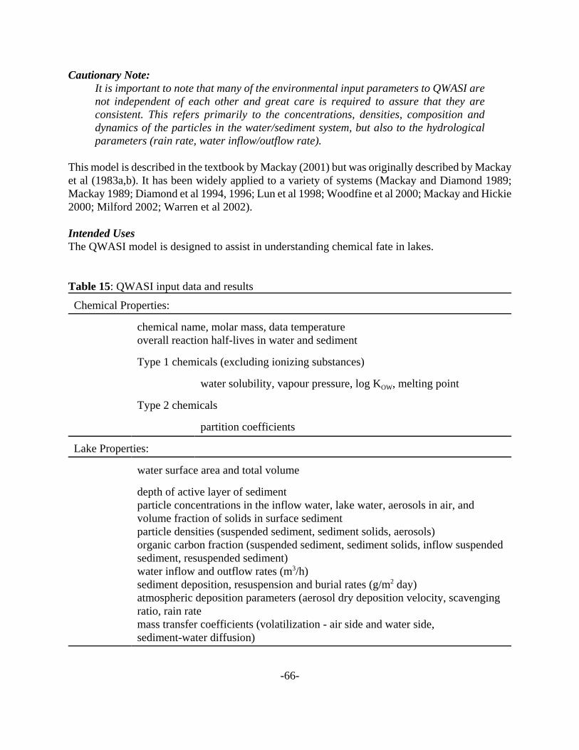
-66-

Cautionary Note: It is important to note that many of the environmental input parameters to QWASI arenot independent of each other and great care is required to assure that they areconsistent. This refers primarily to the concentrations, densities, composition anddynamics of the particles in the water/sediment system, but also to the hydrologicalparameters (rain rate, water inflow/outflow rate).

This model is described in the textbook by Mackay (2001) but was originally described by Mackayet al (1983a,b). It has been widely applied to a variety of systems (Mackay and Diamond 1989;Mackay 1989; Diamond et al 1994, 1996; Lun et al 1998; Woodfine et al 2000; Mackay and Hickie2000; Milford 2002; Warren et al 2002).

Intended UsesThe QWASI model is designed to assist in understanding chemical fate in lakes.

Table 15: QWASI input data and results


chemical name, molar mass, data temperature overall reaction half-lives in water and sediment


water solubility, vapour pressure, log KOW, melting point

Type 2 chemicals


Lake Properties:

water surface area and total volume

depth of active layer of sediment particle concentrations in the inflow water, lake water, aerosols in air, andvolume fraction of solids in surface sediment particle densities (suspended sediment, sediment solids, aerosols) organic carbon fraction (suspended sediment, sediment solids, inflow suspendedsediment, resuspended sediment) water inflow and outflow rates (m3/h) sediment deposition, resuspension and burial rates (g/m2 day) atmospheric deposition parameters (aerosol dry deposition velocity, scavengingratio, rain rate mass transfer coefficients (volatilization - air side and water side,sediment-water diffusion)

-67-

Emissions and Inflows:

direct discharges to the lake concentration in inflow water and in air

Model output includes:

Z and D values fugacities, concentrations and amounts in each compartment details of process rates a summary diagram

4.3.11 AQUAWEB (Version 1.0)

Model OverviewAQUAWEB provides site-specific estimates of chemical concentrations in organisms of aquaticfood webs from chemical concentrations in the water and the sediment (Arnot and Gobas 2004). Themodel is presented in rate constant format for assessing the bioaccumulation of non-ionichydrophobic organic chemicals at steady-state. For zooplankton, aquatic invertebrates and fish themodel calculates rates of chemical uptake from the water and the diet and rates of chemicalelimination to the water, feces and the “pseudo” loss mechanism of growth dilution. Reliablemetabolic transformation rate data can also be included as a mechanism of chemical elimination.AQUAWEB is a modification of a previous model (BIO version 1.0; Gobas 1993). Key revisionsinclude: (i) a new model for the partitioning of chemicals into organisms, (ii) kinetic models forpredicting chemical concentrations in algae, phytoplankton and zooplankton, (iii) new allometricrelationships for predicting gill ventilation rates in a wide range of aquatic species, and (iv) amechanistic model for predicting gastrointestinal magnification of organic chemicals in a range ofspecies. The performance of both versions has been evaluated using empirical data from threedifferent freshwater ecosystems involving 1019 observations for 35 species and 64 chemicals. Table16 lists the limited number of site-specific data inputs required by AQUAWEB.

Intended UsesAQUAWEB is intended to estimate chemical concentrations and associated bioconcentration factors(BCF), bioaccumulation factors (BAF) and biota-sediment accumulation factors (BSAF) ofnon-ionic hydrophobic organic chemicals. The model is useful for assessing exposure and risks ofchemicals in the water and sediment to aquatic ecosystems and higher trophic level organisms thateat aquatic species (i.e., fish) including humans. The model is limited in calculating chemicalconcentrations in species of aquatic macrophytes, algae, phytoplankton, zooplankton, invertebrates,and fish of different trophic levels. Site-specific measurements can be included to evaluate modelperformance.

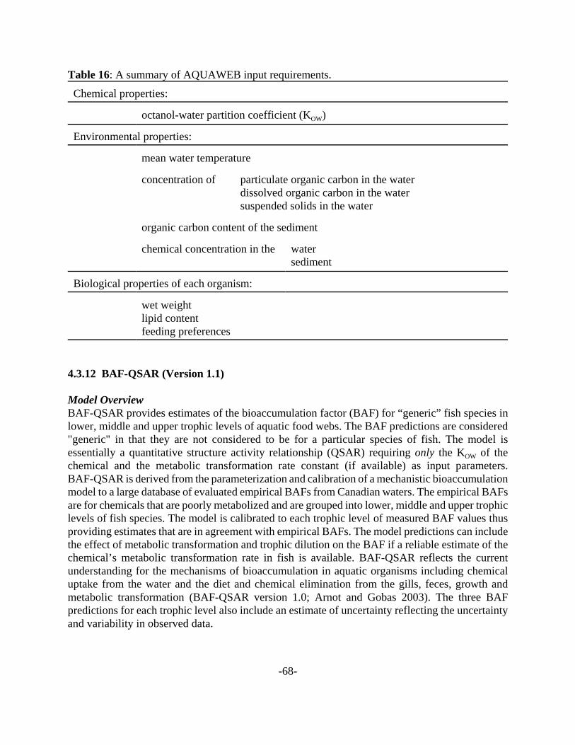
-68-

Table 16: A summary of AQUAWEB input requirements.

Chemical properties:

octanol-water partition coefficient (KOW)

Environmental properties:

mean water temperature

concentration of particulate organic carbon in the waterdissolved organic carbon in the watersuspended solids in the water

organic carbon content of the sediment

chemical concentration in the watersediment

Biological properties of each organism:

wet weightlipid contentfeeding preferences

4.3.12 BAF-QSAR (Version 1.1)

Model OverviewBAF-QSAR provides estimates of the bioaccumulation factor (BAF) for “generic” fish species inlower, middle and upper trophic levels of aquatic food webs. The BAF predictions are considered"generic" in that they are not considered to be for a particular species of fish. The model isessentially a quantitative structure activity relationship (QSAR) requiring only the KOW of thechemical and the metabolic transformation rate constant (if available) as input parameters.BAF-QSAR is derived from the parameterization and calibration of a mechanistic bioaccumulationmodel to a large database of evaluated empirical BAFs from Canadian waters. The empirical BAFsare for chemicals that are poorly metabolized and are grouped into lower, middle and upper trophiclevels of fish species. The model is calibrated to each trophic level of measured BAF values thusproviding estimates that are in agreement with empirical BAFs. The model predictions can includethe effect of metabolic transformation and trophic dilution on the BAF if a reliable estimate of thechemical’s metabolic transformation rate in fish is available. BAF-QSAR reflects the currentunderstanding for the mechanisms of bioaccumulation in aquatic organisms including chemicaluptake from the water and the diet and chemical elimination from the gills, feces, growth andmetabolic transformation (BAF-QSAR version 1.0; Arnot and Gobas 2003). The three BAFpredictions for each trophic level also include an estimate of uncertainty reflecting the uncertaintyand variability in observed data.

-69-

Intended UsesThe model is intended to estimate the bioaccumulation factor (BAF) of non-ionic organic chemicalsin three general trophic levels of fish (i.e., lower, middle and upper). Thus it provides genericestimates in the absence of site-specific measurements or estimates. The model can be used topredict dietary concentrations for higher trophic level predators (e.g., birds and mammals) includinghuman exposure concentrations from fish in their diet. The model has been used to categorizechemicals for their potential to bioaccumulate in aquatic food webs. BAF-QSAR can also be usedin the derivation of water quality guidelines and total maximum daily loadings by relating internalconcentrations of organic chemicals in upper trophic fish species to corresponding concentrationsin the water.

4.3.13 STP Model (Version 2.10)

Model OverviewThe STP model estimates the fate of a chemical present in the influent to a conventional activatedsludge plant as it becomes subject to evaporation, biodegradation, sorption to sludges and to loss inthe final effluent. The most critical and uncertain variable is the biodegradation rate constant andits dependence on biomass concentration. This version of the model allows the use of either degradation half-lives or the Ready test results.As with all other CEMN models, half-life data may be taken from property estimation software suchas EPI Suite, however, monitoring data is to be preferred. Arnot et al (2005) provide guidance onthis issue.

Treatment now includes the possibility of lagoons. The treatment plant is specified as a series of upto 3 tanks or lagoons. For tanks with aeration, surface volatilization is now included in addition tothe volatilization due to the bubbling. The four fates for the system and for each tank individuallyare given as pie charts. To chart other results, or to produce more visually appealing charts, theoutput should be saved to a file and charted using spreadsheet software. The required input data aregiven in Table 17.

This model was based on the work of Clark et al (1995).

Intended UsesThis model is useful for establishing the general features of a new or existing chemical's behaviour,in a sewage treatment plant. It is not intended as an accurate simulation of chemical fate in a specificplant, rather it is a screening level model which seeks to estimate the likely proportions of thechemical which leave the system by biodegradation, in sludge, by evaporation, and in the wateroutflow. These proportions are dictated by both the physical chemical properties of the substanceand the characteristics of the treatment plant. The effect of varying chemical properties such ashalf-lives and operating conditions can be readily explored.

-70-

Table 17: STP (version 2.10) input data and results


chemical name, temperature, molar mass

biodegradation data as half-lives in a primary clarifier, aeration vessel, finalsetting tank, aerated and facultative lagoon or as the Ready test result


water solubility, vapour pressure, log KOW

Type 2 and 3 chemicals


Treatment Plant Properties:

number of tanks influent flow and VSS concentration gas and liquid phase mass transfer coefficients for each tank or lagoon

for each tank or lagoon

- area and depth- biomass fraction of VSS- sludge VSS concentration- outflow (ML)VSS concentration- aeration rate, if applicable- recycled fraction, if applicable- removed fraction, if applicable

Model output includes:

Z and D values steady state phase concentrations process stream fluxes relative amounts of chemical that are likely to be stripped or volatilized,

sorbed to sludge, biodegraded, and discharged in the effluent summary diagrams and charts

-71-

5 ASPECTS OF INTERPRETING MODEL RESULTS

5.1 Understanding the Model Results

Every model produces results that are a unique combination of the model assumptions and the inputparameters. Some types of results are produced by many multimedia models. For example, therelative amounts (or percent) of chemical in each environmental medium.

The percentage shows where most of the chemical is likely to be found. This can indicate in whichmedium effects are most likely to be experienced.

This is also useful in considering the importance of individual media half-lives. It has beensuggested that if less than 5 % of the substance is present in a medium then the half-life in thatmedium can be estimated as infinite without significantly changing the model results for the othermedia.

Another common model result is concentration. Concentrations are calculated for eachenvironmental medium, often in a variety of units, including both wet and dry weight. If anevaluative environment, or emission rate has been used, these concentrations should not becompared to measured concentrations. Any similarity would be coincidental. In the case of anevaluative environment, or emission rate, these concentrations should be compared to concentrationsof other chemicals under the same model conditions. If actual environment and emission rate dataare used, then comparing the concentrations to measured values will be instructive. There are a fewtypical reasons for the modelled and measured concentrations to not be in agreement. These includesuch issues as measurements not reflecting an average for the area modelled, and emission rate databeing incomplete.

The concentration data can be useful when considering where to monitor. A very low calculatedconcentration may suggest that monitoring will be futile. Generally monitoring is most effectivewhen C is high and detection is more reliable.

Many models provide chemical flux values for each modelled process. These are useful inunderstanding chemical movement within the modelled environment and for identifying theimportant processes and model inputs. These help to focus future research on those concepts wherethe most may be gained.

The relative amount lost by each removal process is given in many cases. Care must be taken inreading these results to note whether it is the percentage of the total removed or the percentage ofthe total removed in that medium. Knowledge of the relative importance of each removal processcan focus attention on key processes.

-72-

5.2 Uncertainty and Variability in Environmental Fate Models

A model is necessarily a simplified representation of a real system composed of equations andparameters describing the complex processes experienced by a chemical in the environment. Theequations describe quantitatively the natural processes being modelled, while the parameters, whichinclude chemical properties, discharge or emission data, and landscape parameters, describe relevantproperties of the specific scenario under investigation. As a result of the mathematicalapproximations and the uncertainty and variance in the parameters, a calculated quantity such as aconcentration can not be expected to agree exactly with a measured value. The best that can beachieved is the comparison of a distribution of model values with a distribution of measured values.Ideally, the distribution should overlap. In this section we discuss how distributions of model valuescan be obtained, thus expressing model outcome uncertainty.

The need for uncertainty and sensitivity analyses of model outcome has been long recognised (Slob1994; Jager and Slob, 1995; Cowan et al 1995; Mackay et al 1996a; Vermeire et al 1997; Barnthouseet al 1998; Bennett et al, 1999).

Uncertainty is a measure of the knowledge of the magnitude of a parameter or result. Uncertaintycan be reduced by research, i.e., the parameter value can be refined.

Variance is a measure of the heterogeneity of a landscape parameter or the inherent variability ina chemical property. Variance can not be reduced by further research.

Both uncertainty and variability are quantifiable as distributions and are most frequently describedby lognormal distributions. As discussed by Slob (1994), in cases in which uncertainty in inputs toa model are estimated based on expert judgment, the choice of a lognormal distribution to describeuncertainty is both warranted and advantageous.

An uncertainty in a chemical property such as solubility in water may be described as follows. Asolubility in water may be reported as 50 mg/L but it can be difficult to measure low valuesaccurately. Different workers may (and usually do) report different values. For some well-studiedsubstances a critical review has been undertaken of all available data and a recommended value isselected based on the reviewers’ perception of the accuracy of the results. It may be reported as 50mg/L ± 30 mg/L implying that the true value probably lies (with say 95% certainty) between 80 and20 mg/L. This can be regarded as a normal distribution with a mean of 50 mg/L and a standarddeviation (SD) of 15 mg/L. By definition, 95% of the data lie approximately within two standarddeviations on either side of the mean for a normal distribution.

In many cases of high uncertainty it is preferable to assume a lognormal distribution to apply, ratherthan a normal distribution as assumed above. Using the above example the base ten log of 50 mg/Lis 1.70. The 95% limits of 80 and 20 mg/L correspond to log values of 1.3 and 1.9, i.e., one is 0.2log units higher and the other is 0.4 log units lower. On a lognormal distribution the SD is thenapproximately 0.15, 2 SDs are 0.3 and the limits are (1.7-0.3) or 1.4 and (1.7+0.3) or 2.0

-73-

corresponding to 25 and 100 mg/L. By using a lognormal distribution the low end is compressed,i.e., 20 becomes 25 and the high end is extended, i.e., 80 becomes 100.

This is very advantageous when the SD is large because a normal distribution can give negativenumbers. For example, if the mean is 50 mg/L and the SD is 30 mg/L, the upper limit is 50 + 2 ×30 or 110 mg/L but the lower limit it 50 - 2 × 30 or -10 mg/L which is physically impossible. Byusing a log normal distribution the mean may be 50 mg/L (i.e., 1.7) and if 2 SDs are 0.4 the loglimits are 2.1 and 1.3, then the corresponding solubility values are 125 and 20 mg/L. With alognormal distribution it is impossible to obtain a negative value. For this reason it is generallypreferable to use lognormal distributions in environmental models, especially when there is largeuncertainty.

Note that the SD above of 0.3 corresponds to a constant factor of 100.3 or 2.0 on either side of themean. It is convenient to regard lognormal distributions as plus or minus a factor whereas normaldistributions are plus or minus an absolute quantity. This factor can be termed a “confidence factor”which is a slight misnomer because it is really a “lack of confidence factor”, large valuescorresponding to greater uncertainty and thus less confidence (Macleod et al 2002). If a confidencefactor of Cf is suggested along with a mean X, then the distribution is between XCf and X/Cf. If theSD is F then 2F is log Cf or Cf is 102F. In some cases natural (base e) logarithms are used and Cf ise2F.

The model user should make a judgement as to the confidence factor based on the range of reportedvalues and experience. When there are multiple input parameters each one can be assigned aconfidence factor. Note that quantities such as a log KOW of 6 are already in logarithmic form so aconfidence factor of 2 implies that the true log KOW value lies between 6.0 plus or minus log 2 or0.31 i.e., 5.7 to 6.3. The range is not 3 to 12. Some quantities such as molar mass are known veryaccurately and there is no need to assign an uncertainty.

The use of confidence factors is advantageous because it is easily understood and conveyed toothers.

Also of concern is the possibility of mistakes, as distinct from errors, in both the parameters and inthe model. The commonest mistake is wrong units, e.g., ng instead of mg or the use of loge (that is,ln) when log10 is intended. Model infidelity is most commonly the result of using a model to describea scenario outside the boundaries of the intentions of the model developers. The model may notproperly represent a key process. It may not include it or the inclusion may involve erroneousassumptions. A water quality model may not include evaporation which can be important for somevolatile substances. Ionization may not be included or its effect may be misrepresented. A key dietitem in a bioaccumulation model may be omitted or metabolism may be wrongly ignored. Theseproblems are usually the result of applying a model to a scenario it was not intended to represent.The user must be alert for any such problems. The best guarantee for avoiding them is close scrutinyof the results and a check of reasonableness.

-74-

5.3 Model Sensitivity

Model sensitivity, S, is a measure of the effect of input parameter uncertainty on a model outcomeor result. This depends on the structure of the model equations and the values of the inputparameters. It is useful to begin by considering the simple case of the effect of a single inputparameter on the chosen outcome.

The effect of changing an individual input variable (I) by a fixed amount ()I) on the output ofinterest (O) can be approximated by the following where )O is the change in the output quantity.

S . ()O/O) / ()I/I) (23)

The quantity S describes the sensitivity of O to small (0.1 to 1%) changes in I. In the limit as )Itends to zero (23) becomes:

S = (MO/O) / (MI/I) = MO /MI I/O = MlnO / MlnI (24)

S is thus the partial derivative of O with respect to I.

For example, a chemical in water may be subject to degrading reactions expressed by a rate constantkD and evaporation with a rate constant kE. The equation for concentration could take the form

C = a / (b + kD + kE)

where “a” has a value of 100 and “b” a value of 20. The estimated value of kD is 5 and kE is 20. Theestimated concentration is thus 100 / (20 + 5 + 20) or 2.2. But kD and kE are both uncertain, saywithin a confidence factor of 2. It is possible that kD is then 10 and kE is 40, thus C is 100 / (20 + 10+ 40) or 1.43. Alternatively, kD could be 2.5 and kE could be 10, thus C would be 100 / (20 + 2.5 +10) or 3.07. The uncertainty in kD alone will tend to cause the mean C to vary from 100 / (20 + 2.5+ 20) or 2.35 to 100 / (20 + 10 + 20) or 2.0, a range of about 0.2. In contrast, the same factor of 2change in kE will cause C to vary from 2.86 to 1.54, a much wider range.

The output, C, is thus more sensitive to kE than it is to kD. If b is larger or kD is small then C becomesquite insensitive to kE and uncertainty in it does not propagate through the equations to affect C.

It is important to appreciate how sensitivities vary because there may be little merit in seeking amore accurate value of kD: its value is of little importance.

Mathematically, we are comparing the partial derivative of C with respect to kE and kD but there isno need to undertake the calculus. A simple method is to calculate C for the mean value of kE andkD then change each one in sequence by a small quantity such as 1% or a factor of 1.01. The newvalues of C are calculated, the differences deduced and the difference expressed as a fraction of themean C.

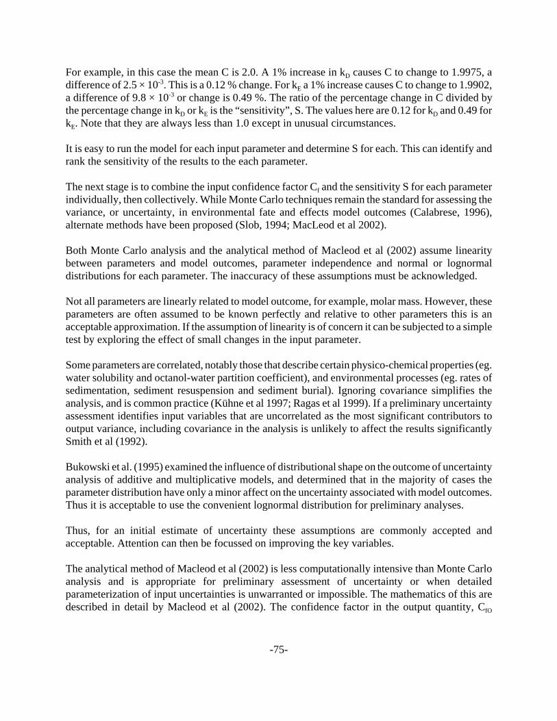
-75-

For example, in this case the mean C is 2.0. A 1% increase in kD causes C to change to 1.9975, adifference of 2.5 × 10-3. This is a 0.12 % change. For kE a 1% increase causes C to change to 1.9902,a difference of 9.8 × 10-3 or change is 0.49 %. The ratio of the percentage change in C divided bythe percentage change in kD or kE is the “sensitivity”, S. The values here are 0.12 for kD and 0.49 forkE. Note that they are always less than 1.0 except in unusual circumstances.

It is easy to run the model for each input parameter and determine S for each. This can identify andrank the sensitivity of the results to the each parameter.

The next stage is to combine the input confidence factor Cf and the sensitivity S for each parameterindividually, then collectively. While Monte Carlo techniques remain the standard for assessing thevariance, or uncertainty, in environmental fate and effects model outcomes (Calabrese, 1996),alternate methods have been proposed (Slob, 1994; MacLeod et al 2002).

Both Monte Carlo analysis and the analytical method of Macleod et al (2002) assume linearitybetween parameters and model outcomes, parameter independence and normal or lognormaldistributions for each parameter. The inaccuracy of these assumptions must be acknowledged.

Not all parameters are linearly related to model outcome, for example, molar mass. However, theseparameters are often assumed to be known perfectly and relative to other parameters this is anacceptable approximation. If the assumption of linearity is of concern it can be subjected to a simpletest by exploring the effect of small changes in the input parameter.

Some parameters are correlated, notably those that describe certain physico-chemical properties (eg.water solubility and octanol-water partition coefficient), and environmental processes (eg. rates ofsedimentation, sediment resuspension and sediment burial). Ignoring covariance simplifies theanalysis, and is common practice (Kühne et al 1997; Ragas et al 1999). If a preliminary uncertaintyassessment identifies input variables that are uncorrelated as the most significant contributors tooutput variance, including covariance in the analysis is unlikely to affect the results significantlySmith et al (1992).

Bukowski et al. (1995) examined the influence of distributional shape on the outcome of uncertaintyanalysis of additive and multiplicative models, and determined that in the majority of cases theparameter distribution have only a minor affect on the uncertainty associated with model outcomes.Thus it is acceptable to use the convenient lognormal distribution for preliminary analyses.

Thus, for an initial estimate of uncertainty these assumptions are commonly accepted andacceptable. Attention can then be focussed on improving the key variables.

The analytical method of Macleod et al (2002) is less computationally intensive than Monte Carloanalysis and is appropriate for preliminary assessment of uncertainty or when detailedparameterization of input uncertainties is unwarranted or impossible. The mathematics of this aredescribed in detail by Macleod et al (2002). The confidence factor in the output quantity, CfO

-76-

depends on the confidence factor in the input quantity (kD and kE in the example) CfI and thesensitivity SI as follows.C CfO fI

SI= | |

orlog | |logC S CfO fI=Note that S can be positive or negative but the positive value or modulus is always used. Clearly ifSI is 1.0 then CfO = CfI. If SI is very small then CfO will be very small. The various values of CfO canbe calculated for each input parameter thus expressing the uncertainty attributable to both the inputparameter and the sensitivity. The ranking of parameter confidence factors is likely to change as aresult.

The final stage is the “add” all of the confidence factors for all of the input parameters. The totalconfidence factor CfT can be approximated as

( ) ( ) ( )ln ln ln ... ln/

C S C S C S CfT f f n fn= + + +⎛⎝⎜

⎞⎠⎟1 1

2

2 2

2 2 1 2

Essentially each SI ln CfI is squared, the sum of squares obtained and the square root taken.

This result is approximate and does not apply when confidence factors are large, but it is usuallyadequate for assessment purposes.

5.4 Model Validity and Fidelity

In the context of risk assessment and regulation, model validation becomes important, howeverenvironmental models can not be validated in the same sense as models of highly reproducibleclosed systems (Oreskes et al 1994; Oreskes 1998). Credibility, however, can be improved bydocumenting examples in which observed and predicted concentrations are compared, as singlevalues or ranges with identification of dominant sources, fate processes, or partitioningcharacteristics. Such comparison studies have been performed on mass balance models of chemicalfate with generally positive results (Devillers et al 1995; Mackay et al 1996c; Bintein and Devillers1996a,b; Koprivnjak and Poissant 1997; MacLeod and Mackay 1999).

The equations in different environmental fate models tend to be very similar (Cowan et al, 1995)indicating a high level of communication and confidence within the research community. In theircomparison of model results, Cowan et al (1995) found that differences were largely attributable todiffering landscape parameters and not to model structure.

( )ln ln/

C S CfT fI

n

=⎛⎝⎜

⎞⎠⎟

=∑ 2 2

2

1

1 2

-77-

5.5 Uncertainty in Dynamic Model Outcomes

In the case of dynamic models, uncertainty and sensitivity analyses are complicated by the changingnature of the system. A process that is initially very important, over time, may assume lessimportance. An analysis such as that presented in section 5.2 can only identify uncertainties in modeloutcome at a single time in a time-dependent fate evaluation. It is difficult and potentiallymisleading to generalize about sensitivities. For dynamic models it is more useful to examinegeneral trends.

When chemical is first introduced to a medium, the “receiving medium”, there is a period of uptakeby the other media, “non-receiving media” during which the removal rates are insufficient to balancethe intermedia transport of chemical into these media. During this time, the model outcome is mostsensitive to the properties and processes of intermedia transport from the receiving medium to thenon-receiving media. In the case of a constant discharge into the receiving medium, after some time,steady-state will be achieved and the results from an analysis such as that in section 5.5.2 will apply.At the other extreme, a single, one-time discharge will not lead to a steady-state scenario. The periodof uptake by the non-receiving media will be followed by a period of clearance during which theadvection and degradation rates will be more important than the intermedia transport rates.

The key consideration is the equilibrium status between the receiving medium and the non-receivingmedia, i.e., their relative fugacities. There is thus a potential for a profound change in sensitivity asthe system approaches or digresses from equilibrium.

This “inspection” method is preferable for dynamic models since it conveys an inherentunderstanding of the model assumptions and the nature of the simulations.

5.6 Temperature Effects

It must be appreciated that most of the input parameters to the models are dependent on temperature.Some reaction rate are especially temperature sensitive. Obviously, if the aim is to model chemicalfate in a specific system and a specific temperature, an attempt should be made to obtain parametervalues appropriate to that temperature.

Most reported data are at 25 /C which is convenient for the laboratory determinations since beingabove ambient indoor temperatures, no refrigeration is required. Environmental temperatures areusually lower on the average and in temperate climates lie in the range of 10 to 15 /C, but extremesare possible.

The temperature correction for reaction rate constants is usually an activation energy that is specificto the conversion process. For microbial kinetics a Q10 is often used, the factor change in rate for a10 /C change in temperature. Microbial kinetics are complicated because the community changeswith temperature thus the organisms operating at 5/C are different from those at 25 /C.

-78-

K K eT ToH R T To

11= − −∆ /( ( ))

Partition coefficients also change with temperature and in a more predictable way. The usualapproach is to estimate the enthalpy change )H associated with the phase-to-phase transfer andemploy an equation of the type

where KT1 and KTo are the partition coefficients at temperature T1 and To and R is the gas constant.The sign of )H can cause confusion and it is easier to deduce whether K increases or decreasesusing LeChateleir’s Principle. For example, for water to air exchange an increase in temperaturepromotes evaporation so K increases, i.e., KT1 > KTo and T1 > To, so )H must be positive orendothermic, i.e., heat is absorbed on evaporation. The Principle states that the system responds toan increase in temperature by seeking to counteract it and absorbing heat which implies evaporation.Enthalpies are particularly large and important for air-solid and air-liquid systems and can be up to100 kJ/mol. For liquid-liquid systems or liquid-solid systems the enthalpy is generally less than 20kJ/mol, but there are exceptions.

Some models such as ChemCAN (version 6.00) use enthaply terms to correct partition coefficientsand TaPL3 (version 3.00) corrects the half-lives. Most models, however, require the user to do thesecorrections manually and enter the temperature corrected values.

5.7 Steady-state v.s. Dynamic Assumptions

Steady-state models assume that neither chemical emissions, nor environmental parameters changein time, and that the sum of the chemical fluxes in and out of the various model compartmentsbalances each other at any time. Whereas this limitation is justified for many model applications,it is not when the temporal variability of chemical fate and exposure is of interest. The use andemission of chemicals is hardly ever constant on any time scale. Similarly, the environment isundergoing constant change, e.g. on a diurnal, seasonal and a multi-year time scale, and manytime-variant environmental factors (e.g. temperature) have an impact on chemical behaviour. Buteven for time-invariant emissions and environments, steady-state assumptions may not be valid. Thisis particularly relevant for chemicals with very slow degradation half-lives, which take a very longtime for establishing steady-state distributions in the environment. To address chemical assessmentsituations that involve a temporal component a Level IV model is required.

5.8 Summary

There are three sources of uncertainty and variance contributing to uncertainty in the outcome frommodels of chemical fate in the environment; chemical properties, landscape properties, and emissiondata. There is an incentive to minimize error and uncertainty in all three. In focussing data researchefforts, sensitivity analyses are helpful but care must be exercised to avoid misleading evidence. Thecost of the effort to define or refine a parameter should be balanced against the expected reductionin outcome uncertainty.

-79-

6 WHERE TO FIND HELP

There are various sources of information on CEMN models and modelling in general. In additionto the information provided here and in the books and journal articles referenced, help may be foundin the readme.txt that accompanies most models, the model’s Help files, and by examining thecalculations displayed in the model, and on CEMN websites

http://www.trentu.ca/cemnhttp://www.rem.sfu.ca/toxicology/http://www.utsc.utoronto.ca/~wania/http://www.trentu.ca/cemc

-80-

7 REFERENCES

Arnot, J. A., Gobas, F. A. P. C. 2004. A Food Web Bioaccumulation Model for Organic Chemicals in AquaticEcosystems. Environ. Toxicol. Chem. 23: 2343-2355.

Arnot, J. A., Gobas, F. A. P. C. 2003. A Generic QSAR for Assessing the Bioaccumulation Potential ofOrganic Chemicals in Aquatic Food Webs. QSAR and Combinatorial Science 22: 337-345.

Arnot, J.A., Mackay, D., Gouin, T. 2005. Development and Application of Models of Chemical Fate inCanada: Practical methods for environmental biodegradation rate estimation. Report to Environment Canada.CEMN Report No. 2005xx. Trent University, Peterborough, Ontario.

Barnthouse, L, Fava, J., Humphreys, K., Hunt, R., Laibson, L., Noesen, S., Norris, G., Owens, J., Todd, J.,Vigon, B., Weitz, K., Young, J., 1998. Life-Cycle Impact Assessment: the State-of-the-Art. Report of theSETAC Life-Cycle Assessment (LCA) Impact Assessment Workgroup. Society of Environmental Toxicologyand Chemistry (SETAC).

BEC (Bonnell Environmental Consulting) 1999a. Characterizing Uncertainty in the Exposure Assessmentof New Substances in Canada. Prepared under contract for the New Substances Division, EnvironmentCanada, March 1999.

BEC (Bonnell Environmental Consulting) 1999b. A Strategy for the Improved Exposure Assessment of NewSubstances in Canada. Prepared under contract for the New Substances Division, Environment Canada,December 1999.

BEC (Bonnell Environmental Consulting) 2001. Conducting the multi-media exposure assessment of newsubstances in Canada. Prepared under contract for the New Substances Division, Environment Canada. July2001.

Bennett, D.H., Kastenberg, W.E., McKone, T.E. 1999. A multimedia, multiple pathway risk assessment ofatrazine: the impact of age differentiated exposure including joint uncertainty and variability. ReliabilityEngineering and System Safety. 63: 185-198.

Beyer, A., Mackay, D., Matthies, M., Wania, F., Webster, E. 2000. Assessing Long-range Transport Potentialof Persistent Organic Pollutants. Environ. Sci. Tech. 34: 699-703.

Beyer, A., Wania, F., Gouin, T., Mackay, D., Matthies, M. 2002. Selecting Internally ConsistentPhysical-Chemical Properties of Organic Compounds. Environ. Toxicol. Chem. 21: 941-953.

Beyer, A., Wania, F., Gouin, T., Mackay, D., Matthies, M. 2003. Temperature Dependence of theCharacteristic Travel Distance. Environ. Sci. Technol. 37: 766-771.

Bidleman, T.F., Harner, T. 2000. “Sorption to Aerosols.” Chapter 10 in Handbook of Property EstimationMethods for Chemicals: Environmental and Health Sciences. Boethling, R.S., Mackay, D. (Eds) CRC Press,Boca Raton, pp. 233-260.

Bintein, S., Devillers, J., 1996a. Evaluating the environmental fate of lindane in France. Chemosphere. 32:2427-2440.

-81-

Bintein, S., Devillers, J., 1996b. Evaluating the environmental fate of atrazine in France. Chemosphere. 32:2441-2456.

Breivik, K., Wania, F. 2003. Expanding the applicability of multimedia fate models to polar organicchemicals. Environ. Sci. Technol. 37: 4934-4943.

Bukowski J, Korn L, Wartenberg D. 1995. Correlated inputs in quantitative risk assessment: The effect ofdistributional shape. Risk Analysis 15: 215-219.

Calabrese, E.J., 1996. Special Issue: Commemoration of the 50th anniversary of Monte Carlo. Hum. Ecol.Risk Assess. 2: 627-1038.

Carson, R. 1962. Silent Spring, Houghton Mifflin, Boston, MA.

CEPA (Canadian Environmental Protection Act). 1999. Canadian Environmental Protection Act, 1999.Statutes of Canada 1999. Chapter 33. Act assented to 14 September 1999. Environment Canada.

Cole, J.G., Mackay, D. 2000. Correlation of Environmental Partitioning Properties of Organic Compounds:The Three Solubilities Approach. Environ. Toxicol. Chem. 19: 265-270.

Cowan C. E., Mackay D., Feijtel T. C.J., van de Meent D., Di Guardo A. Davies J., Mackay N. 1995. “TheMulti-Media Fate Model: A Vital Tool for Predicting the Fate of Chemicals”. Proceedings of a WorkshopOrganized by the Society of Environmental Toxicology and Chemistry (SETAC), SETAC Press, PensacolaFL. pp 78.

Devillers, J.; Bintein, S.; Karcher, W., 1995. Chemfrance: a regional level III fugacity model applied toFrance. Chemosphere. 30: 457-576.

Diamond, M., Mackay, D., Poulton, D., Stride, F. 1994. Development of a Mass Balance Model of the Fateof 17 Chemicals in the Bay of Quinte. J. Great Lakes Res. 20: 643-666.

Diamond, M.L., Mackay, D., Poulton, D.J., Stride, F.A. 1996. Assessing Chemical Behavior and DevelopingRemedial Actions Using a Mass Balance Model of Chemical Fate in the Bay of Quinte. Wat. Res. 30:405-421.

Environment Canada. 2003. Guidance Manual for the Categorization of Organic and Inorganic Substanceson Canada’s Domestic Substances List: Determining Persistence, Bioaccumulation Potential, and InherentToxicity to Non-human Organisms. June 2003. Existing Substances Branch. Environment Canada.

ESB (Existing Substances Branch, Environment Canada). 2003. Guidance Manual for the Categorization ofOrganic and Inorganic Substances on Canada's Domestic Substances List: Determining Persistence,Bioaccumulation Potential, and Inherent Toxicity to Non-human Organisms. June 2003.(http://www.ec.gc.ca/substances/ese/eng/dsl/cat_index.cfm)

Fenner, K., Scheringer, M., MacLeod, M, Matthies, M., McKone, T., Stroebe, M., Beyer, A., Bonnell, M.,Le Gall, A.C., Klassmeier, J., Mackay, D., van de Meent, D., Pennington, D., Scharenberg, B., Suzuki, N.,Wania, F. 2005. Comparing Estimates of Persistence and Long-Range transport Potential among MultimediaModels. Environ. Sci. Technol. xx: xxx-xxx. (Web release: February 2005.)

-82-

Finizio, A., Mackay, D., Bidleman, T., Harner T., 1997. Octanol-Air Partition Coefficient as a Predictor ofPartitioning of Semi-Volatile Organic Chemicals to Aerosols. Atmos. Environ. 31, 2289-2296.

Gobas, F. A. P. C. 1993. A Model for Predicting the Bioaccumulation of Hydrophobic Organic Chemicalsin Aquatic Food Webs: Application to Lake Ontario. Ecological Modelling 1993: 1-17.

Gouin, T., Cousins, I., Mackay, D. 2004. Comparison of Two Methods for Obtaining Degradation Half-lives.Chemosphere. 56: 531-535.

Gouin, T., Mackay, D., Webster, E., Wania, F. 2000. Screening chemicals for persistence in the environment.Environ. Sci. Technol. 34: 881-884.

Government of Canada, 1994. New Substances Notification Regulation. Canada Gazette, part II. Ottawa,March 24th, Vol 129, No. 9

Howard, P. 1989, 1990, 1991, 1993, 1997. Handbook of Environmental Fate and Exposure Data for Organics(Volumes I - V) CRC Press.

Howard, P. 1991. Handbook of Environmental Degradation Rates CRC Press.

Howard, P. 1996. Handbook of Physical Properties of Organic Chemicals CRC Press.

Hung, H., Lee, C.S., Wania, F., Blanchard, P., Brice, K. 2005. Measuring and simulating atmosphericconcentration trends of polychlorinated biphenyls in the Northern hemisphere. Atmos. Environ. (Submitted.)

Jager D.T., Slob, W. 1995. Uncertainty analysis of the Uniform System for the Evaluation of Substances(USES). Report no. 679102027. RIVM. Bilthoven, The Netherlands.

Jury, W.A., Spencer, W.F., Farmer, W.J. 1983. Behaviour assessment model for trace organics in soil. I.Model description. J. Environ. Qual. 12: 558-564.

Koprivnjak, J.F., Poissant, L. 1997. Evaluation and application of a fugacity model to explain the partitioningof contaminants in the St. Lawrence River Valley. Water, Air, and Soil Pollution 97: 379-395.

Kühne, R., Breitkopf, C., Schüürmann, G. 1997. Error propagation in fugacity Level III models in the caseof uncertain physicochemical compound properties. Environ. Toxicol. Chem. 16: 2067-2069.

Lakaschus,S.,Weber, K., Wania, F., Bruhn, R., Schrems, O. 2002. The air-sea equilibrium and time trend ofhexachlorocyclohexanes in the Atlantic Ocean between the Arctic and Antarctica. Environ. Sci. Technol. 36:138-145.

Lun, R., Lee, K., De Marco, L., Nalewajko, C., Mackay, D. 1998. A Model of the Fate of PolycyclicAromatic Hydrocarbons in the Saguenay Fjord. Environ. Toxicol. Chem. 17: 333-341.

MacLeod, M., Mackay, D. 1999. An assessment of the environmental fate and exposure of benzene and thechlorobenzenes in Canada. Chemosphere 38: 1777-1796.

-83-

MacLeod, M., Fraser, A., Mackay, D. 2002. Evaluating and Expressing the Propagation of Uncertainty inChemical Fate and Bioaccumulation Models. Environ. Toxicol. Chem. 21: 700-709.

Mackay, D. 1989. Modelling the Long Term Behaviour of an Organic Contaminant in a Large Lake:Application to PCBs in Lake Ontario. J. Great Lakes Res. 15: 283-297.

Mackay, D. 2001. Multimedia Environmental Models: The Fugacity Approach - Second Edition. LewisPublishers, Boca Raton, pp.1-261.

Mackay, D., Boethling, R.S. (Eds.) 2000. Handbook of Property Estimation Methods for Chemicals:Environmental and Health Sciences. CRC Press, Boca Raton.

Mackay, D., Diamond, M. 1989. Application of the QWASI (Quantitative Water Air Sediment Interaction)Fugacity Model to the Dynamics of Organic and Inorganic Chemicals in Lakes. Chemosphere. 18:1343-1365.

Mackay, D., Hickie, B. 2000. Mass Balance Model of Sources, Transport, and Fate of PAHs in Lac SaintLouis, Quebec. Chemosphere.41: 681-692.

Mackay, D., Joy, M., Paterson, S. 1983a. A Quantitative Water, Air, Sediment Interaction (QWASI) FugacityModel for Describing The Fate of Chemicals in Lakes. Chemosphere. 12: 981-997.

Mackay, D., Paterson, S., Joy, M. 1983b. A Quantitative Water, Air, Sediment Interaction (QWASI) FugacityModel for Describing the Fate of Chemicals in Rivers. Chemosphere. 12: 1193-1208.

Mackay, D., Di Guardo, A., Paterson, S., Kicsi, G., Cowan, C.E. 1996a. Assessing the Fate of New andExisting Chemicals: A Five Stage Process. Environ. Toxicol. Chem. 15: 1618-1626.

Mackay, D., Di Guardo, A., Paterson, S., Cowan, C.E. 1996b. Evaluating the Environmental Fate of a Varietyof Types of Chemicals Using the EQC Model. Environ. Toxicol. Chem. 15: 1627-1637.

Mackay, D., Di Guardo, A., Paterson, S., Kicsi, G., Cowan, C.E., Kane, D.M. 1996c. Assessment of ChemicalFate in the Environment Using Evaluative, Regional and Local-Scale Models: Illustrative Application toChlorobenzene and Linear Alkylbenzene Sulfonates. Environ. Toxicol. Chem. 15: 1638-1648.

Mackay, D., Shiu, W.Y., Ma, K.C. 2000. Physical-Chemical Properties and Environmental Fate andDegradation Handbook. CRCnetBASE 2000, Chapman & Hall CRCnetBASE, CRC Press LLC., Boca Raton,FL. (CD-ROM.)

Mackay, D., Paterson, S., Shiu, W.Y. 1992. Generic models for evaluating the regional fate of chemicals.Chemosphere. 24: 695-717.

Mackay, D., Stiver.W.1991. Predictability and environmental chemistry. In: R. Grover A.J. Cessna (Eds.).Environmental Chemistry of Herbicides Vol.II CRC Press.Boca Raton FL pp. 281-297.

McLachlan, M., Czub, S.G., Wania, F. 2002. The influence of vertical sorbed phase transport on the fate oforganic chemicals in surface soils. Environ. Sci. Technol. 36: 4860-4867.

-84-

Meyer, T., Wania, F., Breivik, K. 2005. Illustrating sensitivity and uncertainty in environmental fate modelsusing partitioning maps. Environ. Sci. Technol. (In press)

Milford, L. 2002. A Multi-Segment Modelling Approach to Describe the Fate of PCBs in Two River Systemsin Southern Ontario. Masters thesis, Watershed Ecosystems Graduate Program, Trent University,Peterborough, Ontario.

Oreskes, N., 1998. Evaluation (not validation) of quantitative models. Environmental Health Perspectives.106 (Suppl. 6): 1453-1460.

Oreskes, N., Shrader-Frechette, K., Belitz, K., 1994. Verification, validation, and confirmation of numericalmodels in the earth sciences. Science. 263: 641-646.

Platts,J., Butina, A.D., Abraham, M.H., Hersey. A.1999. Estimation of molecular linear free energy relationdescriptors using a group contribution approach. J. Chem. Inf. Comput. Sci. 39: 835-845.

Ragas MJ, Etienne RS, Willemsen FH, van de Meent D. 1999. Assessing model uncertainty for environmentaldecision making: A case study of the coherence of independently derived environmental quality objectivesfor air and water. Environ Toxicol Chem 18: 1856-1867.

Scheringer, M., Wania, F. 2003. Multimedia models of global transport and fate of persistent organicpollutants. In: H. Fiedler (Ed.) The Handbook of Environmental Chemistry Vol.3 Part O Springer-VerlagBerlin Heidelberg pp.238-269.

Seth, R., Mackay, D., Muncke, J. 1999. Estimating of Organic Carbon Partition Coefficient and Its Variabilityfor Hydrophobic Chemicals. Environ. Sci. Technol. 33: 2390-2394.

Shiu, W.Y., Ma, K.C., Varhanickova, D., Mackay, D. 1995. Chlorophenols and Alkyphenols: A Review andCorrelation of Environmentally Relevant Properties and Fate in an Evaluative Environment. Chemosphere.29: 1155-1224.

Slob, W., 1994. Uncertainty Analysis in Multiplicative Models. Risk Analysis. 14: 571-576.

Smith AE, Ryan PB, Evans JS. 1992. The effect of neglecting correlations when propagating uncertainty andestimating the population distribution of risk. Risk Analysis 12: 467-474.

Vermeire, T.G., Jager, D.T., Bussian, B., Devillers, J., den Haan, K., Hansen, B., Lundberg, I., Niessen, H.,Robertson, S., Tyle, H., van der Zandt, P.T.J., 1997. European Union System for the Evaluation of Substances(EUSES). Principles and structure. Chemosphere. 34: 1823-1836.

Verschueren, K. 2001. Handbook of Environmental Data on Organic Chemicals, Fourth Edition. Wiley.(CD-ROM)

Wania, F., Breivik, K, Persson, N.J., McLachlan, M.S. 2005. CoZMo-POP2-a fugacity-based dynamicmulti-compartmental mass balance model of the fate of persistent organic pollutants. EnvironmentalModelling & Software. (In review)

-85-

Wania, F., Su, Y. 2004. Quantifying the global fractionation of polychlorinated biphenyls. Ambio. 33:161-168.

Wania, F. 2004. Schadstoffe ohne Grenzen - der Ferntransport persistenter organischer Umweltchemikalienindie Kälteregionen der Erde. GAIA. 13: 174-183.

Wania, F. 2003. Assessing the potential of persistent organic chemicals for long-range transport andaccumulation in polar regions. Environ. Sci. Technol. 37: 1344-1351.

Wania, F., Daly, G.L. 2002. Estimating the contribution of degradation in air and deposition to the deep seato the global loss of PCBs. Atmos. Environ. 36: 5581-5593.

Wania,F., Persson, N.J., DiGuardo, A., McLachlan, M.S. 2000. CoZMo-POP. A fugacity-basedmulti-compartmental mass balance model of the fate of persistent organic pollutants in the coastal zone.WECC-Report 1/2000.

Wania,F., McLachlan, M.S. 2001. Estimating the influence of forests on the overall fate of semi volatileorganic compounds using a multimedia fate model. Environ. Sci. Technol. 35: 582-590.

Wania, F., Mackay, D. 1999. Global chemical fate of "-hexachlorocyclohexane. 2 Use of a global distributionmodel for mass balancing source apportionment and trend predictions. Environ. Toxicol. Chem. 18:1400-1407.

Wania, F., Mackay, D. 2000. The global distribution model. A non-steady state multi-compartmental massbalance model of the fate of persistent organic pollutants in the global environment. Technical Report andComputer Program (www.utsc.utoronto.ca/~wania).

Wania, F., Mackay, D., Li, Y.-F., Bidleman, T.F. 1999. "-hexachlorocyclohexane. 1 Evaluation of a globaldistribution model. Environ. Toxicol. Chem. 18: 1390-1399.

Wania, F., Mackay, D.1995. A global distribution model for persistent organic chemicals. Sci. Total Environ.160/161 211-232.

Warren, C.S., Mackay, D., Bahadur, N.P., Boocock, G.B. 2002. A Suite of Multi-Segment Fugacity ModelsDescribing the Fate of Organic Contaminants in Aquatic Systems: Application to the Rihand Reservoir, India.Water Research 36:4341-4355.

Webster E., Mackay, D., Wania, F. 1998. Evaluating Environmental Persistence. Environ. Toxicol. Chem.17: 2148-2158.

Webster, E., Mackay, D. 2003. Defining Uncertainty and Variability in Environmental Fate Models. CEMCReport No. 200301. Trent University, Peterborough, Ontario.

Mackay, D., Webster, E., Woodfine, D., Cahill, T., Doyle, P., Couillard, Y., Gutzman, D. 2003. TowardsConsistent Evaluation of the Persistence of Organic, Inorganic and Metallic Substances. Human andEcological Risk Assessment (HERA). 9(6): 1445-1474.

-86-

Webster, E., Cowan-Ellsberry, C.E., McCarty, L. 2004a. Putting science into PBT evaluations. Environ.Toxicol. Chem. 23: 2473-2482

Webster, E., Mackay, D., Di Guardo, A., Kane, D., Woodfine, D. 2004b. Regional Differences in ChemicalFate Model Outcome. Chemosphere. 55: 1361-1376.

Woodfine D.G., Seth R., Mackay D., Havas M. 2000. Simulating the Response of Metal Contaminated Lakesto Reductions in Atmospheric Loading Using a Modified QWASI Model. Chemosphere. 41: 1377-1388.

Woodfine, D. Mackay, D. 2001. Evaluation of Partitioning and Persistence of Organic Substances onEnvironment Canada's Domestic Substances List. Report to Environment Canada. CEMC Report No. 200105.Trent University, Peterborough, Ontario.

-87-

APPENDIX A: COMMONLY USED VARIABLES AND THEIR UNITSSubscripts for environmental media

A or 1 air

W or 2 water

E or 3 soil or earth

S or 4 sediment

F or 5 or B fish or biota

P or 6 suspended particles in water

Q or 7 aerosols

T system total

R the gas constant 8.314 PaAm3 mol-1 K-1

T temperature K

A area m2

V volume m3

Kij partition coefficient between media i and j dimensionless unless otherwise noted

KOW octanol-water partition coefficient dimensionless

KOA octanol-air partition coefficient dimensionless

KAW air-water partition coefficient dimensionless

PS vapour pressure (solid state) Pa

CS aqueous solubility (solid state) mol/m3

PL vapour pressure (liquid state) Pa

CL aqueous solubility (liquid state) mol/m3

H Henry’s law constant Pa m3/mol

D density kg/L

J half-life hours

t time hours

f fugacity Pa

C concentration mol/m3

M mass or amount of chemical mol

E emission mol/h

-88-

Z fugacity capacity mol m-3 Pa-1

D fugacity rate constant mol Pa-1 h-1

TO overall residence time

TR or P residence time due to degrading reactions, persistence

TA residence time due to advection

LRT long-range transport

S model sensitivity

Cf confidence factor

Order of magnitude values of transport parameters for Level III calculations. (Mackay 2001)

Parameter Symbol Suggested typical value

Air side MTC over water kVA 3 m/h

Water side MTC kVW 0.03 m/h

Transfer rate to higher altitude US 0.01 m/h (90 m/y)

Rain rate (m3rain/m2area.h) UR 9.7x10-5 m/h (0.85m/y)

Scavenging ratio Q 200000

Vol. Fraction aerosols vQ 30x10-12

Dry deposition velocity UQ 10.8 m/h (0.003 m/s)

Air side MTC over soil kEA 1 m/h

Diffusion path length in soil Y3 0.05 m

Molecular diffusivity in air BMA 0.04 m2/h

Molecular diffusivity in water BMW 4.0x10-6 m2/h

Water runoff rate from soil UWW 3.9x10-5 m/h (0.34 m/y)

Solids runoff rate from soil USW 2.3x10-8 m3/m2 h (0.0002 m/y)

Water side MTC over sediment kSW 0.01 m/h

Diffusion path length in sediment Y4 0.005 m

Sediment deposition rate UDP 4.6x10-8 m3/m2 h (0.0004 m/y)

Sediment resuspension rate URS 1.1x10-8 m3/m2 h (0.0001 m/y)

Sediment burial rate UBS 3.4x10-8 m3/m2 h (0.0003 m/y)

Leaching rate of water from soil to groundwater

UL 3.9x10-5 m3/m2 h (0.34 m/y)

-89-

Typical intermedia transfer D value equations for Level III calculations.

Compartments Process D Values

air(1)- water(2) diffusion DV = 1/(1/kVA A12 ZA + 1/kVW A12 ZW)

rain dissolution DRW = A12 UR ZW

wet deposition DQW = A12 UR Q vQ ZQ

dry deposition DQD = A12 UQ vQ ZQ

D12 = DV + DRW2 + DQW2 + DQD2

D21=DV

air(1) - soil(3) diffusion DE = 1/(1/kEAA13ZA +Y3/(A13(BMAZA + BMWZW))

rain dissolution DRW3 = A13 UR ZW

wet deposition DQW3 = A13 UR Q vQ ZQ

dry deposition DQD3 = A13 UQ vQ ZQ

D13 = DE + DRW3 + DQW3 + DQD3

D31=DE

soil(3) - water(2) soil runoff DSW = A13 UEW ZE

water runoff DWW = A13 UWW ZW

D32 = DSW + DWW

D23 = 0

sediment(4) - water(2) diffusion DY = 1/(1/kSWA24ZW + Y4/BMWA24ZW)

deposition DDS = UDP A24 ZP

resuspension DRS = URS A24 ZS

D24 = DY + DDS

D42 = DY + DRS

reaction either bulk phase i or sum of all phases

DRi = kRi Vi ZiDRi = E (kRij Vij Zij)

advection bulk phase DAi = Gi Zi or Ui Ai Zi

Aij is the horizontal area between media i and j

-90-

APPENDIX B: FREQUENTLY ASKED QUESTIONS

CEMC Software Installation

Q: Why can’t I install your software on my computer?

A: If you are using either Windows NT or Windows 2000, our software will not install on yourcomputer. Our software is designed to work with Windows 98 and XP.

Q: What operating systems will the models run on?

A: The models are known to run on Windows 98 and Windows XP. If you are having problemsinstalling with these operating systems, it could be due to the degree of permission you have toinstall software if working on a networked computer. Look to your IT people for permission toinstall new programs that modify the system directory.

Q: Do any of your models operate on a Mac?

A: All of the downloadable models are self-extracting zip files which may not run on a Mac, but feelfree to try.

General Modelling

Q: Is there a guidance manual or users guide for the software available from the CEMC?

A: We do not produce manuals for each model, instead we try to include sufficient information inthe model labels and layout, and in the "Help" screens. Also, each model contains reference to apaper that may provide extra useful information.

Q: I am running two models but not getting the same results.

A: Are the processes included in each model the same? Is one of the two inappropriate for your task?If you are running two versions of the same model, check the newer model for improvements listedin the readme.txt, in the model, and on the website. Are the inputs consistent?

-91-

Q: How can I print the diagram?

A: All printing of model results is done from the main screen, under the “Print” button. Here theTables and/or the Diagram may be selected. For some software, a few simple charts are alsoavailable.

Q: How can I save the results diagram to a file?

A: To save the diagram to file from our software, use the “Print Screen” button on your keyboardto save you screen to the computer’s clipboard. Using “Alt” + “Print Screen” will capture the imageof only the prominent window (i.e., the diagram form). Paste into a document and save thedocument.

Q: There seems to be a bug in this model…

A: Please check the known bug report on the website. If it is not listed there, please e-mail us toinform us of the problem.

Q: Are any of the CEMC models are used for regulatory risk assessment of chemicals in NorthAmerica?

A: It is our understanding that our EQC model and the Level I, II, III series (with emphasis onLevels II and III) are used both in Canada and in the USA. For details on how these models are usedyou should contact Environment Canada and the US EPA directly. In particular, try to get a copyof the “Guidance Manual for the Categorization of Organic and Inorganic Substances on Canada'sDomestic Substances List” (June 2003) from the Existing Substances Branch of EnvironmentCanada. This should give you a good starting point.

Q: Is there a multimedia model available on your site that does uncertainty and sensitivity analysis?

A: Most of the models available at the CEMC are set up to run with a single set of properties foreach chemical, i.e., sensitivity and uncertainty analysis have to be done by hand. We are currentlyworking on Level II and Level III Batch Mode software and they will simplify the process. They arenot yet ready for public release.

-92-

Q: How can I determine long-range transport when using a model such as ChemCAN which doesnot provide for this?

A: Assuming an average (uni-directional) windspeed of 14.4 km/h, long-range transport, LRT, canbe calculated as

LRT in air = 14.4 * ResTime * mass fraction of chemical in air

where ResTime is the overall residence time. This is what is done in the TaPL3 model.

The assumption of a constant uni-directional wind is a very broad one. One of the criticisms of thismethod has been that for very persistent, volatile chemicals, the distance calculated can be manytimes the Earth's circumference. In addition, a single temperature is assumed - also unrealistic overlarge distances. So, the intent is not to calculate place-to-place transport potential but rather to assigna relative, quantitative value to the potential for LRT.

Chemical Data

Q: Where is it possible to find the partition coefficients for Type 2 chemicals? Can they be derivedfrom known values?

A: Normally we use Type 1 properties if at all possible. Type 2 and 3 properties provide amechanism where the Type 1 properties are not measureable. (Type 2 and 3 data are actuallycalculated by the model when Type 1 data are input.) Our best data source is the Mackay et al (2000)handbooks. These are a compilation of data in the scientific literature. If you are still havingdifficulties finding data, you may need to rely on QSARs (Quantitative Structure ActivityRelationships, more properly known as QSPRs, Quantitative Structure Property Relationships) tomake estimates. Beware that using QSAR estimates of properties adds another level of uncertaintyto your results!

Q: I don't have a value for the vapour pressure, is there a way to enter the Henry's Law Constantdirectly?

A: This is possible in some models, ChemCAN, for example. Otherwise, if you have a watersolubility, S, and the Henry's Law Constant, H, it is possible to calculate a vapour pressure (Mackay2001). See Section 3.5.1.

-93-

Q: I am dealing with chemicals that are completely miscible and chemicals that are gaseous, andthese chemicals don't seem to fit into any of the three categories of chemical types. How can I modelthese chemicals?

A: Multimedia models are most useful for substances which partition into more than oneenvironmental medium. For substances which partition exclusively (or nearly exclusively) to asingle medium such as air, a multimedia model is not needed; the properties of the chemical aloneare sufficient to understand its behaviour.

Q: For the chemical input, what does the temperature input represent?

A: This input is the temperature at which the chemical’s properties were measured.

Q: In the model results, why are the times for the chemical to be in a medium shorter than predictedby the half-lives?

A: The half-life in each medium is the degradation half-life only and does not include transporteither to other media, or out of the system.

Q: Where can I find chemical data to model site temperatures from -30C to +20C?

A: There are reviews of the temperature dependence of physico-chemical property data in theliterature. The best journals to search are the Journal of Physical and Chemical Reference Data,Environmental Toxicology and Chemistry, and Environmental Science and Technology. Oneexample is Ma et al (2001) which gives the temperature dependence of the aqueous solubility ofselected chlorobenzenes and chlorotoluenes in the Journal of Chemical Engineering Data.Handbooks also contain some data of this type, especially recent editions. Alternatively, contact aresearcher active in this area directly for advice.

Environmental Data

Q: What is the size difference between local-scale and far-field (or regional) model environments?

A: The surface area for a local-scale evaluation is less than 10000 km2 (100x100 km) but typicallyless than a few kilometres in each direction. Far-field models should not be used for areas of lessthan 10000 km2 or larger than about 1000000 km (1000 x 1000 km). Areas larger than 1000000 kmshould be sub-divided before evaluation to avoid over-simplifying the heterogeneity of eachenvironmental compartment.

-94-

Q: What exactly are volume fractions?

A: This parameter is the fraction of a compartment - by volume - which is comprised of the specificsub-compartment. These values are used in calculating the Z-value. For example, the volumefraction of sediment solids is the fraction of the sediment which is solid particles (ie. not water)

Q: I would like some information on parameterization of environmental volumes. Different defaultenvironmental parameters were reported in old papers from those now used in model software.

A: The environmental properties in earlier models were selected to be typical of southern Ontario.For EQC, values were selected to be more useful internationally. In the Level III model it is possibleto change the volumes to suit your requirements. It is important to note that it is the responsibilityof the user to ensure that all input values are correct. We provide a couple of environments so thatthere is something there to start with. However, the values in the database can be changed - we havenot locked these environments - so we can't make any guarantees about the results the user will seefor a particular environment name.

EQC - Q&A

Q: What are the assumed environmental parameters for the EQC?

A: If you are running an old version of EQC, this information is not apparent. However, you mayfind it useful to download version 2.02 of the EQC model, as it has been upgraded to allow the userto view all of the environmental properties and all of the calculations in the model.

Q: How can I specify my own custom environment when using EQC?

A: EQC does not allow for user specified environments. To model specific locations, use the LevelI, Level II, Level II set of models. They contain approximately the same calculations as EQC butallow the user to change the environmental properties. In addition, for Level III-type calculations,we have the ChemCAN model which was designed for regional analysis of the fate of chemicals inthe environment.

Q: Why are there different volumes of soil and sediment in the Levels I and II as compared to LevelIII for EQC?

A: Partitioning in the soil and sediment is assumed to be primarily to the solid fraction and since,for Level I and II, the volume fractions of these environmental media are not normally defined, thevolumes used are equal to the volume of the solid phase in the Level III calculation where thevolume fractions are defined. This means that the Level II concentration in soil or sediment should

-95-

be treated as a dry weight concentration and compared to the Level III concentration in the solidfraction.

Q: Is EQC OK for modelling surfactants? Or do you have any caveats about fugacity modelling ofthis group of chemicals?

A: Treat surfactants as a Type 2 chemical.

Q: What does the advection process in the water and sediment refer to? Is this simply removalthrough dilution?

A: Advection is not dilution. Advection in water is loss of chemical as the river water flows out ofthe modelled area and is replaced by inflowing water. The inflowing water may also contain thechemical. Advection in sediment is the permanent burial of sediment as particles deposit out of thewater column and the deeper layers of sediment become unavailable for chemical exchange with themodelled system.

Q: What is the difference between EQC and QWASI?

A: EQC is regional-scale, generic and unmodifiable environment, multimedia model with definedwater and land cover. QWASI is an aquatic model suitable for modelling lakes with an emission tothe water. A user-defined chemical concentration in the air above a waterbody contributes tochemical in the water and sediment. There is no landmass associated with the waterbody in QWASI.The lake properties are modifiable to represent any lake system. By considering “lakes” connectedin series, a river may be simulated.

Q: How can I scale the results from EQC to model around a stack site?

A: The EQC standard environment is probably not the best one to use for estimating the partitioningof your compound. It assumes proportions of the four environmental media which may not berepresentative of the area you are concerned with.

In the area you are interested in, what fraction of the surface is covered by water? Use this with thetotal area in the EQC standard environment. Estimate a representative value for the depth of thewater. The EQC standard values for the depths of soil and sediment are likely sufficiently close. Askthe local weather office for a rain rate and scale the related transport velocities. These can have alarge effect. Depending on the properties of your compound, these changes in the environmentalproperties may or may not have a significant effect on the proportions of the compound in eachmedium.

-96-

Once you have the fractions of compound in each medium from the Level III software you can applythem to the small area around the stack. If you have the measured concentration in the air, that canbe used to calculate the concentration in each of the other media.

Q: I am having a problem running EQC. What are my options?

A: Try using the Level I, II and III models. They are based on the same equations as EQC.

FoodWeb - Q&A

Q: Can the FoodWeb model be used for river ecosystems?

A: This model can be used for a river ecosystem but it will not treat the water flow effects, i.e., itwill assume that your water is a single, well-mixed compartment.

Q: Is there a newer version of the FoodWeb model available to download?

A: A software version has been written and is being tested in preparation for release.

ChemCAN - Q&A

Q: How many Canadian regions are there in ChemCAN and how were they decided?

A: There are 24 regions of Canada in the ChemCAN model. The regional divisions of Canada werebased on the ecozones identified by Environment Canada and with consideration of the distributionof population and industrial activity, political boundaries, drainage basins, and climate to give areasof sufficiently homogeneous ecological conditions such that meaningful assessments of chemicalfate can be conducted.

Q: What is the maximum or minimum areas you can use for a region?

A: For surface areas of a region it is not recommended going less than about 10000 km2 (100x100km) or larger than about 1000000 km (1000 x 1000 km).

Q: I am estimating that 1000 kg/year is released in Canada, and I am using the "average" region ofCanada. I am therefore dividing the 1000 kg/year by 24, because the region is 1/24th the size ofCanada. Is this an appropriate method of using this region?

-97-

A: No. ChemCAN is intended for region-specific evaluations. The “Average” region is amathematical average of the values for each of the 24 specific regions of Canada and was designedto allow an investigation of regional differences. For a non-region specific evaluation, use the “EQCstandard environment” included in the ChemCAN database with an emission proportional to thepopulation density of southern Ontario compared to Canada as a whole. The releases will bedifferent in each region and the fate will be different. Using the "average" region and an "average"emission will give a result unrepresentative of any region of Canada to a degree dependent upon thechemical.

Q: I have a tested value for my chemical in the water (0.5 ng/L), is this the most appropriate valueto enter for advection inflow concentration of water?

A: That depends on where this sample was taken. The correct value should be representative of therivers flowing into the region of interest.

Q: Can I run the model iteratively to estimate the advection inflow concentration in air?

A: Yes. In the absence of concentration data for the upwind region running the model assuming azero inflow air concentration, to get an initial concentration in the air and then re-running the modelusing this concentration for the inflow air this is a good estimation method. Either the calculatedconcentration in the air may be used or some fraction (such as 1/4) of that value may be used.

Q: In ChemCAN, are the values used for the temperature dependence coefficients and the oneparameter method of estimating partitioning to aerosols standard defaults that can be used for allType 1 chemicals, or do these need to be changed for each chemical? How can these values beestimated?

A: These are chemical specific inputs and the “default” value are provided for use with thosechemicals where the values are not known. It is best to use chemical-specific values if possible. Formore information, refer to the the work of Beyer et al (2002) on temperature dependence and to thesource of the partitioning to aerosols correlation (Finizio et al 1997).

Q: How can I save the diagram to an image file?

A: To save the diagram to file from our software, use the "Print Screen" button on your keyboardto save you screen to the computer’s clipboard. Using Alt + "Print Screen" will capture the imageof only the prominent window (i.e., the diagram form). Paste into a document and save thedocument.

-98-

TaPL3 - Q&A

Q: I don't have data for the enthalpy energy requirements for KOW and KAW in TaPL3. Is there a wayto bypass having to enter these numbers?

A: If your chemical data were collected at the same temperature as your modelled environment, theequation collapses such that the value of the enthalpy has no effect. Of course, this is quiteunrealistic since the environment is seldom at the temperature of the lab. There are a couple of“default” sets of values for the enthalpies based on categories of chemicals. As a first pass, broadgeneralization, you could use -20 : 55 which were assigned to the X - hypothetical chemical for KOW: KAW However, these values are based on a limited set of similar substances and so may beinappropriate for your substances. For chemical-specific data refer to Beyer et al (2002).

Q: TaPL3 does not account for advective losses. However the substance is deposited over an area(not a point). Can you provide me suggestions on how to infer the size of deposition area?

A: TaPL3 is intended for the evaluation of persistence. Since advection moves chemical to anotherregion, it was decided that it was more honest to include only degradation. Air to surface (water orsoil) deposition happens over the entire simulated area.

STP - Q&A

Q: Where can I get half-life data for this model?

A: Preferably, use monitoring data. If this is not available, property estimation models such asEPIWIN may be helpful.

QWASI - Q&A

Q: How does QWASI differ from the other CEMC models, such as EQC?

A: The QWASI model is specific to aquatic systems and does not contain a soil (landmass)compartment.

Levels I, II, III - Q&A

Q: When running Level I, if the soil compartment is reduced to zero, it merely "amplifies" the samerelative compartmentalization in the remaining media as when the soil was present. Is this ok?

-99-

A: The odd thing you will notice is that the concentration in soil is still calculated. This is becausethe concentration is the product of the Z and the fugacity, neither of which (in Level I) depend onthe presence of the medium. If you consider the "total" chemical present in the system to be the sumof that in air, water, fish, suspended particles, and sediment and calculate the percentages based onthis new total, you should see results identical to the "no soil" run. Your thinking is correct.

Q: When modifying the area should I also change the advective flow residence time? It seems thatif I reduce the linear dimension in the direction of the wind by 10 fold and reduce the total area by100-fold, that the advective flow residence times should be reduced proportionally. If all else isunchanged, reducing the size of the box should reduce the residence time, I would think. However,I find that if I leave the advective residence times unchanged but do change the dimensions, theproportion of chemical input into air that exits the air due to advection is unchanged. When I reducethe advection proportionally, the amount advected out of the air increases dramatically. Both resultsseem counter-intuitive.

A: The “Advective Flow Residence Time” is the time that the air or water will spend in the definedregion. You are right in thinking that this is related to the size of the region. We do not automaticallymodify these values when the areas are changed because we believe that the user knows better thanwe do what shape the region is and how that relates to the prevailing wind direction. For example,if the region is rectangular and not square, the residence time of the air will depend on whether thewind blows in the short or the long direction and thus affect the residence time of the air.

By reducing the areas, the volumes of all media are reduced. If the residence times (and all othervalues) are unchanged, the flow rate of the air (volume/res time) is reduced. The D value (flow rate× Z value) is also reduced. All the fugacities are increased! The concentrations (fugacities × Zvalues) are increased. Therefore... the loss rates (fugacity × D value) and amounts (conc × volume)are not affected.

When the "Advective Flow Residence Time" is reduced, the air is effectively being removed morequickly and any chemical in the air is also being removed more quickly.

Q: In your Level III program results under the tab “Phase Properties” the amounts are 87.8 % to thebulk water phase and 11.9 % to the sediment phase. However, in the losses section, the amount is98.6% to the water phase for percent of total losses. What is the information in these two columnsand why is there a difference?

A: In your case, of the chemical remaining in the system, 87.8% is in the water and 11.9% is in thesediment. Of the chemical removed from the system, 98.6% is removed by processes in the waterphase.

-100-

Q: How is the Level III in your models different from the Level III available through the EPI Suiteprogram.?

A: We were not involved with the creation of the EPI Suite program so we cannot say for sure. Theirdocumentation is your best source of information on the equations and assumptions they use. Theequations used in our models are available under the “Display Calculations” button in the top rightcorner of the main window.

CEMC DOS Models

Q: I am trying to use the old DOS models from the website but I am having no luck. After I choosemy scenarios and hit enter, the program seems to just stop. Please help!

A: There are two possible causes. - First, this program sends all output to the default printer. Make sure you have a printer connected.- Second, some newer equipment will not run these models. Check to see if there is a newerWindows version of this model available on the website, you may want to download this and seeif this works for you.

License Issues

Q: Can we make your models available on our website?

A: No, we would prefer that you do NOT distribute out models, but please feel free to link to ourwebsite.

Q: Can we have the code for your models?

A: No, the source code for our models is NOT available. These models are licenced software. Pleaserefer to the licence agreement for details. The models are transparent by design, thus allowing youfull access to visually inspect the model calculations.

References for FAQs

Beyer, A., Wania, F., Gouin, T., Mackay, D., Matthies, M. 2002. Selecting Internally ConsistentPhysical-Chemical Properties of Organic Compounds. Environ. Toxicol. Chem. 21: 941-953.

Finizio, A., Mackay, D., Bidleman, T., Harner T. 1997. Octanol-Air Partition Coefficient as a Predictor ofPartitioning of Semi-Volatile Organic Chemicals to Aerosols. Atmos. Environ. 31: 2289-2296.

Ma. J.H.Y, Hung, H., Shiu, W.-Y., Mackay, D. 2001. Temperature Dependence of the Aqueous Solubilityof Selected Chlorobenzenes and Chlorotoluenes. J. Chem. Eng. Data 46: 619-622.

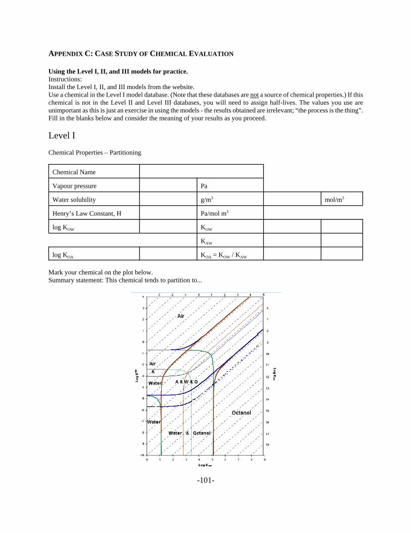
-101-

APPENDIX C: CASE STUDY OF CHEMICAL EVALUATION

Using the Level I, II, and III models for practice.Instructions: Install the Level I, II, and III models from the website.Use a chemical in the Level I model database. (Note that these databases are not a source of chemical properties.) If thischemical is not in the Level II and Level III databases, you will need to assign half-lives. The values you use areunimportant as this is just an exercise in using the models - the results obtained are irrelevant; “the process is the thing”.Fill in the blanks below and consider the meaning of your results as you proceed.

Level I

Chemical Properties – Partitioning

Chemical Name

Vapour pressure Pa

Water solubility g/m3 mol/m3

Henry’s Law Constant, H Pa/mol m3

log KOW KOW

KAW

log KOA KOA = KOW / KAW

Mark your chemical on the plot below.Summary statement: This chemical tends to partition to...

-102-

Z Values

Z (air)

Z (water)

Z (soil)

Z (sed)

Summary Statement: Fugacity capacities suggest that this chemical has the greatest affinity for ...

fugacity (Pa)

partitioning (%) concentration (mol/m3)

Air

Water

Soil

Sediment

Comment on relative amounts and relative concentrations...

Level II

Half-lives (h)

Air

Water

Soil

Sediment

Suspended Particles

Fish

Aerosols

Based on Level I results, to what extent is this chemical present in the medium where its half-life is greatest?

-103-

fugacity (Pa)

partitioning (%) concentration (mol/m3)

Air

Water

Soil

Sediment

Compare these results to the Level I results.

loss by advection (%) loss by reaction (%)

Air

Water

Soil -

Sediment -

Total

Which is the most important removal process?

Persistence (hours)

Attributable to reaction

Attributable to advection

Total Persistence

How important are the advective processes in determining the total persistence?Repeat the above calculations with a second chemical and compare the Persistence values for the two chemicals.

LRT estimate

assume square region, 2 km high

distance = square root of total area

wind speed = distance / residence time of air

total mass in air (mol)

total rate of removal by reaction (mol/h)

LRT = wind * total mass in air / total rate of removalby reaction

Repeat with your second chemical and compare the LRT values for the two chemicals.

-104-

Level III

Emission (kg) Inflow Concentrations

Air

Water

Soil

Sediment

Bulk compartments fugacity (Pa) partitioning (%) concentration (mol/m3)

Air

Water

Soil

Sediment

Persistence (hours)

Attributable to reaction

Attributable to advection

Total Persistence

How important are the advective processes in determining the total persistence?Repeat with your second chemical and compare the persistences for the two chemicals.

LRT estimate

assume square region, 2 km high

distance = square root of total area

wind speed = distance / residence time of air

total mass in air (mol)

total rate of removal by reaction (mol/h)

LRT = wind * total mass in air / total rate of removalby reaction

Repeat with your second chemical and compare the LRT values for the two chemicals.Take a few minutes to read through the calculations as displayed in Level III. Follow one of the input properties (e.g.organic carbon fraction in soil) through the calculations to see how it impacts an output parameter (e.g. total persistence).

-105-

APPENDIX D: LEVEL I CALCULATION OF DDT IN A WATER BODY SUCH AS A LAKE OR HARBOUR.

A lake is 10 km by 10 km by 50 m deep and contains sediment of 5 % organic carbon (OC) anddensity 2 g/cm3 to a depth of 5 cm. Suspended particulate matter (SPM) has a concentration of 20mg/L (density 2 g/cm3) and 10 % organic carbon. Biota (eg. fish) are present at 5 mg/L (density 1g/cm3) of lipid content 10 %. The lake contains 8000 kg of DDT. Calculate its equilibriumdistribution at 25 °C in the lake and in the air to a height of 1000 m above the water.

Properties at 25 °C

MW Solubility (g/m3) Vapour Pressure Pa Log KOW

DDT 354 0.0031 0.00002 6.2

HCB 285 0.005 0.0023 5.5

DCB 147 83 90 3.4

Answer

(1) Calculate Volumes

Air VA = (10 x 1000)2 x 1000 = 1011 m3

Water VW = (10 x 1000)2 x 50 = 5 x 109 m3

Sediment VS = (10 x 1000)2 x 0.05 = 5 x 106 m3

SPM VP = VW x 20 x 10-6 / 2 = 5 x 104 m3

Biota VB = VW x 5 x 10-6 = 25000 m3

(2) Calculate Z values (mol/m3APa)

ZA = 1 / RT = 1 / (8.314 x 298) = 4.04 x 10-4

ZW = CS / PS = (0.0031 / 354) / 0.00002 = 0.438

ZS = ZW x KSW = ZW x OC x 0.4 x KOW x Density OC is organic carbon content

-106-

= 0.438 x 0.05 x 0.4 x 1.58 x 106 x 2 = 27700

ZP = ZW x KPW (similarly) = 55400

ZB = ZW x lipid content x KOW = 69200

(3) Calculate VZ and GVZ

air water sediment particles biota

40.4 2190 138500 2770 1730 (all x 106)Total = 145230 x 106

(4) Calculate fugacity etc.

Amount = 8000 kg = 8000 x 1000 / 354 = 22600 mol = M

f = M / GVZ = 22600 / 145230 x 106 = 1.56 x 10-7 Pa.

C = Zf mol/m3 C g/m3 Mass = VC / 1000 kg % C in other units

air 6.2 x 10-11 2.2 x 10-8 2.2 0 22 ng/m3

water 6.8 x 10-8 2.4 x 10-5 120 1.5 24 ng/L

sediment 0.0043 1.53 7599 95.4 0.75 :g/g

particles 0.0086 3.04 152 1.9 1.5 :g/g

biota 0.0107 3.8 95 1.2 3.8 :g/g

100

Note bioconcentration factor 3.8 / 24 x 10-6 = 158000 = lipid content x KOW

Repeat the Level I calculation for either hexachlorobenzene (HCB) or 1,4 dichlorobenzene

(DCB) with the properties given earlier .

-107-

APPENDIX E: LEVEL II CALCULATION FOR DDT IN A LAKE.

The same lake receives a total input of 10 kg/h of DDT. Do a level II calculation assuming thefollowing:

Residence times:

air 1 hour

water 240 hours

Reaction half-lives:

air infinite

water 1 year

sediment 2 years

susp sediment 1 year

biota 4 months

We calculate D values as follows:

Rates (Df)

Advection air G = 1011 m3/h D = GZ = 40.4 x 106 20.04

water G = 5 x 109 / 240 D = GZ = 9.1 x 106 4.6

Reaction note k = 0.693 / half life D = VZk

air D = 0 0

water D = 5 x 109 x 0.438 x 0.693 / 8760 = 0.17 x 106 0.01

sediment D = 5 x 106 x 27700 x 0.693 / 17520 = 5.49 x 106 2.8

susp. sediment D = 0.22 x 106 0.1

fish D = 0.41 x 106 0.2

Total D 55.7 x 106 Total 28.2

Emission = 10 x 1000 / 354 = 28.25 mol/h = Df

-108-

ˆ f = 5.07 x 10-7 Pa

Concentrations and masses can be calculated as before.

Total amount is 73700 mol = 26000 kg

Residence time or persistence = 26000 / 10 = 2600h = 108 days

Note relative importance of D values

The rates are calculated as Df, and are given on the previous page. They add to the total input rate.Repeat the Level II calculation for either HCB or DCB emitted at 10 kg/h assuming the same

residence times but the following half lives.

HCB DCB

air infinite infinite

water 1 year 1 day

sediment 2 years 2 days

susp sediment 1 year 1 day

fish 4 months 12 hours

-109-

APPENDIX F: LEVEL III CALCULATION OF DDT IN A LAKE.

From information on intermedia transport rates, the following D values are estimated. This is a

fairly time consuming task, so it is not given in detail here. Note: air is 1, water is 2 and sediment

is 3.

Emission into water 10 kg/h or 28.25 mol/PaAh

D value for air - water transfer D12 = 15 x 106 mol/PaAh

D value for water - air transfer D21 = 10 x 106

D value for sediment - water D32 = 30 x 106

D value for water - sediment D23 = 50 x 106

Advection and reaction D values DA1 and DA2, and DR2 and DR3 are as before. We write mass

balance equations for each compartment.

Air

f2 D21 = f1 (D12 + DA2)

ˆ f1 = f2 x 10 x 106 / (15 + 40.4) x 106 = f2 x 0.18

Sediment

f2 D23 = f3 (D32 + DR3)

ˆ f3 = f2 x 50 / (30 + 5.49) = f2 x 1.41

Water

E + f1 D12 + f3 D32 = f2 (DA2 + DR2 + D21 + D23)

Note: DR2 should include reaction in suspended sediment and fish, i.e., a total of 0.8 x 106

f2 = E / (DA2 + DR2 + D21 + D23 - 0.18 D12 - 1.41 D32)

= 28.25 / (9.1 + 0.8 + 10 + 50 - 0.18 x 15 - 1.41 x 30)106

-110-

= 1.13 x 10-6

f1 = 0.2 x 10-6 f3 = 1.6 x 10-6

Check that total net losses equal inputs.

Loss from air f1 DA1 = 8.22

Loss from water f2 (DA2 + DR2) = 11.20

Loss from sediment f3 DR3 = 8.78 Total = 28.20 (close enough)

Note that now the fugacity (and concentration and amount) in water has increased by a factor of 2.2,

air has fallen by a factor of 2.5, and sediment has increased by a factor of 3.1. These changes are

caused by the intermedia transport resistances. The relative importance of the loss processes thus

changes. Previously, in Level II, the loss from air was DA1f1 or 20.5 mol/h. It is now 8.2 mol/h.

Water was 4.9; it is now 11.2. Sediment has increased from 2.8 to 8.8 reflecting the larger amounts

in water and sediment, caused by the resistance to evaporation.

These Level III fugacities and concentrations should be comparable to monitored values, i.e., some

validation is possible.

This Level III could be repeated for HCB and DCB using the following intermedia values (all x 106)

HCB DCB

D12 5 1.2

D21 4 1

D32 10 0.4

D23 12 0.5

-111-

Y = DF x CTVwater (Kd + 2m)

where,

Y = critical soil concentration (mg/kg)DF = dilution factor (default = 50)CTVwater = critical threshold value for water(mg/L)Kd = soil-water partition coefficient 2m = soil moisture content (default = 41%from Level III model)

APPENDIX G

Groundwater Model for Assessing the Potential Transport of New Substances to SurfaceWater Bodies via Recharge (from CCME 1996)

To determine whether a new substance released to soil is at a critical concentration that will resultin a surface water concentration exceeding a CTV the following generic equation can be usedmodeified from Appendix D of CCME (1996).

The rational for the above equation is presented in the following sections.

Numerous studies have shown that sorption of organics by soils is highly correlated with the organicmatter content (e.g., Chiou et al. 1979, Hassett et al. 1980). Chiou (1989) presents evidence that thelinearity of sorption with organic contaminant concentration and correlation with soil organic mattercontent reflect dissolution of the organic contaminant into the soil organic matter phase -- asopposed to sorption to organic matter surfaces. Normally a Freundlich isotherm is fitted to thesorption data:

Cs = Kd × Cw1/n [1]

where Cs = concentration in solid phase (mg/kg)Kd = distribution coefficientCw = concentration in aqueous phase (mg/L) n = empirical constant

For most non-ionic organics n=1 and sorption is a linear function of equilibrium solutionconcentration up to 60% to 80% of its water solubility (Hassett and Banwart 1989). The relationship

-112-

between solution concentrations and the sorbed concentration is described in equation 1. Therelationship between total soil concentration and soil solution concentration can be derived usinga simple method based only on mass ratio of water over soil considerations.

Consider a unit dry mass of soil, Ms, at field capacity moisture content 2m defined by

2m = Mw/Ms [2]

where Mw = mass of waterMs = dry mass of soil

The soil is contaminated by a chemical to a concentration Y (mg kg-1 dry mass basis) and thechemical is partitioned between solid and aqueous phases of the moist soil per:

Kd = Cs/Cw [3]

By mass balance we have:

Y × Ms = (Cs × Ms) + (Cw × Mw) [4]

Rearranging [2] and substituting in [4]:

Y × Ms = (Cs × Ms) + (Cw × 2m × Ms)

and

Y = Cs + (Cw × 2m)

Cs = Y - (Cw × 2m) [5]

Substituting [5] into [3]:

Kd = Y - (Cw × 2m)Cw

which, after rearrangement yields

Y = Cw(Kd + 2m) [6]

Dissociating Organic Contaminants

Equilibrium partitioning isotherms effectively describe the behaviour of non-dissociating organiccontaminants in soils. This description may be extended to dissociating organic contaminantsprovided sorption of both the dissociated and non-dissociated forms is understood and easily treated.

-113-

These conditions are met for some weak organic acids, such as chlorophenols, because only the non-dissociated form is appreciably sorbed. Like many other anions, the phenate generated by thedissociation of the parent chlorophenol is mobile in soils. Because of this difference, chlorophenolpartitioning can be predicted from the concentration of the non-ionized form, which is a functionof pH. The pH-dependent distribution coefficient can then be calculated (Schellenberg et al. 1984)as the product of the partitioning coefficient for the chlorophenol and the proportion of the non-ionized form:

Kd = Koc × Foc × Q [7]

where Koc = organic carbon-normalized coefficient for non-ionized chlorophenolFoc = fraction of organic carbon in soilQ = proportion of chlorophenol in non-ionized form

It is important to note that experimental data that nominate Koc have been referenced to theconcentration of non-dissociated chlorophenol.

Q is derived from the equilibrium acidity expression for the chlorophenol:

Q = 1/(1 + Ka/[H+]) [8]

where Ka = acidity constant

Substituting [7] and [8] into [6]:

Y = Cw[(Koc × Foc/(1 + Ka/[H+]) + 2m]

The additional information required to calculate the total soil concentration of a weak acidcontaminant in equilibrium with the desired water quality is therefore:

! soil pH,! acidity constant of the contaminant, and! partition coefficient for the non-ionized acid.

Organic contaminants that protonate to cationic forms (e.g., amines) cannot be accommodated bythe above treatment because, in soils, cations are competitively sorbed on colloids, which vary withsoil type.

Development of the Dilution Factor (DF)

Equilibrium partitioning concepts predict the concentration of a non-polar organic chemical in waterdraining from a soil at a contaminated site. Estimating the effect of this recharge on groundwaterquality requires that dilution be considered. Dilution of an organic contaminant in recharge watermay be described by considering the contaminant fluxes in recharge and groundwater to an effective

-114-

mixing depth as it leaves the contaminated site. The vertical contaminant flux through the vadosezone is given by:

Qcv = Csw × R × A [1]

where Qcv = vertical contaminant flux mg yr-1

Csw = concentration of contaminant in soil water (recharge), mg/m3

R = recharge, m/yr

A = area of contaminated site, m2

Neglecting lateral dispersion, the horizontal contaminant flux in groundwater is approximated byQch = Cgw [(W × B × q) + (R × A)] [2]

where Qch = horizontal contaminant flux, mg/yr

Cgw = concentration of contaminant in groundwater, mg/m3

W = width of contaminated zone, m

B = effective mixing depth in aquifer, m

q = Darcy velocity of aquifer, m/yr

Applying mass balance considerations, contaminant transport in the vadose and saturated zones isset equal:

Csw × R × A = Cgw [(W × B × q) + (R × A)] [3]

And a dilution factor (DF) may be defined as:

DF = Csw/Cgw = [(W × B × q) + (R × A)]/R × A [4]

Which reduces to

DF = (W × B × q/R × A) + 1 [5]

By definition

A = W × L [6]

where L = length of contaminated site, m

-115-

Substituting [6] into [4] yields

DF = (B × q/R × L) + 1 [7]

Finally, estimates of the Darcy velocity are usually obtained by considering the saturated hydraulicconductivity and gradient:

q = Ksat × i [8]

where Ksat = saturated hydraulic conductivity, m yr-1

i = hydraulic gradient (dimensionless)

A working formula for estimating expected steady state dilution for an organic contaminant ingroundwater is therefore:

DF = (B × K × i/R × L) + 1 [9]

The basis for the general estimation of dilution effects in groundwater observed at the down-gradientboundary of a contaminated site is formed in equation 9. Appropriate ranges for effective mixingdepth, hydraulic conductivity and gradient, recharge, and site length are developed below.

Dilution Factor Parameter Ranges

Effective Mixing Depth

On the lower end of the range, the effective mixing depth (B) is restricted by the practicalconsideration that a generic unconfined aquifer targeted for protection at the human drinking waterguideline must have sufficient yield to be exploitable as a potable source. Taken alongside welldesign requirements, it is assumed that B must equal or exceed 1 m.

An upper limit for B will be set by the balance between rates of vertical dispersion and lateraltransport over the length of the contaminated site. Effective mixing depth would be expected to bemaximized by high recharge, low groundwater velocity, high permeability and large site lengths.However, these conditions do not necessarily co-occur — high recharge and permeability usuallyare associated with high velocity. A further practical constraint on the observed concentration of acontaminant in water drawn from a potable well is the effect of the slotted or perforated zone on"depth averaging" of well water. Slotted or perforated zones of potable wells can be expected toexceed the thickness of the contaminated zone in many instances. In such cases the well will tendto function as a mixing cell over the depth of the slotted or perforated zone.

These considerations suggest that an effective mixing depth between 1 and 5 m is reasonable.Because high yield aquifers (which minimize requirements for slotted zone thickness) are soughtas potable sources a modal effective thickness is nominated downrange at 2 m.

-116-

Hydraulic Conductivity of Aquifer

Common Canadian aquifers have textures ranging from silty sands (fine) to intermediate gravels(coarse) (Brown 1967). Freeze and Cherry (1979) give typical hydraulic conductivity values for siltysands to intermediate gravels in the range of 10-6 to 10-2 m sec-1. A majority of productive aquifersare sands to fine gravels (Brown 1967). Such aquifers would have a hydraulic conductivity (Ksat) inthe region of 10-4 m sec-1.

Hydraulic Gradient

The hydraulic gradient is a dimensionless quantity describing the steepness of the water potentialgradient. In unconfined aquifers it is roughly equivalent to the gradient of the water table. Thehydraulic gradient is assumed to vary between 0.5 and 5% at most contaminated sites. In the absenceof a systematic data review the modal gradient was assumed equal to the mean of the boundingestimates.

Recharge

Methodology

Recharge is rarely measured directly but can be calculated by a water balance approach (Hillel1971):

S = P - ET - R - U [10]

where S = storage in soilP = precipitationET = evapo-transpirationR = rechargeU = surface runoff

Over long periods of time (e.g., years) S = 0 and

R = P - ET - U [11]

Meteorological monitoring stations throughout Canada make direct measurements of precipitationand these have been compiled into thirty-year means (Environment Canada 1982), which providean excellent source of data for water balance purposes. Actual evapo-transpiration estimatescomputed from class A pans and local-to-regional water balances are also available (Fisheries andEnvironment Canada 1978). Unfortunately, runoff calculated from gauging rivers includes bothrecharge and surface runoff (in this case runoff is defined for the entire drainage basin and thestorage term includes subsurface drainage). Such runoff estimates are also affected by heavy

-117-

precipitation in mountainous regions that do not represent contaminated sites, which typically occurat lower elevations.

Because surface runoff in cultivated areas is an erosion hazard, it is normally managed against andrepresents a small proportion of the total water balance (Hillel 1971). Therefore, problems causedhere by lack of surface runoff measurements can be circumvented by computing recharge andsurface runoff (R + O) estimates from precipitation and evapotransportation and allowing for amaximum surface runoff:

R + U = P - ET [12]

Surface runoff is not likely to represent more than a quarter of the total amount of recharge andsurface runoff at a majority of populated locations in Canada and may be close to zero in somelocations (C. Maulé, pers. comm.). Factors affecting the relative proportions of drainage and surfacerunoff include vegetal cover, surface soil condition, slope, intensity of precipitation events, andextent of ice lensing during spring snowmelt. Many of these factors vary greatly on local rather thanregional scales. In the absence of a systematic data summary, surface runoff is assumed to average15% of the total amount of recharge and surface runoff:

R = 0.85 (P - ET) [13]

Precipitation data were obtained from Environment Canada (1982) and actual evapo-transpirationdata taken from small scale maps prepared by Fisheries and Environment Canada (1978). Wheremore than one precipitation monitoring station was available for a given location the mean of allobservations was used.

Results

Recharge calculated from equation [13] for a range of locations spanning most climatic typescommon to populous areas of Canada. Estimates range from nearly 1 m in maritime regions to nearzero in some prairie locations. Small, negative values of drainage occur in some arid locations.These likely are caused by underestimation of precipitation by standard gauges (Fisheries andEnvironment Canada 1978) and, in any event, deviate from more direct estimates of drainage inthese locations by only a few mm (C. Maulé 1993, pers. comm.).

Extreme values of recharge (>1 m) occur, or are expected to occur, in maritime regions of highrainfall -- particularly exposed coastal areas of British Columbia and Newfoundland. However, inthese areas groundwater protection concerns are in part mitigated by:

! the relatively infrequent occurrence of potable, unconfined, shallow aquifers (related to thepreponderance of poorly permeable igneous and metamorphic bedrock types); and

! low human population densities, which should indicate low contaminated site frequency.

-118-

Recharge in high precipitation regions is likely overestimated in equation [13] because surfacerunoff and interflow is increased by:

! the generally greater relief existing in these areas of Canada, and

! the frequency and duration of precipitation can exceed the soil infiltration capacity.

Recharge in populated areas of Quebec surrounding the St. Lawrence river has been estimated torange to about 0.3 m (L. Martel 1994, pers. comm.).

For the screening purposes here recharge was taken to vary between 0.005 and 0.5 m yr-1. A modalrecharge of 0.2 m yr-1 was chosen to reflect the abundance of contaminated sites in the Windsor toQuebec City corridor.

Site Length

The length of a contaminated site in the present context is merely the surface lateral dimensionparallel to the direction of groundwater flow. The lower limit could be a retail gas station (with awidth as small as 15 m). The upper limit could include local-to-regional contamination phenomenaproduced by severe atmospheric deposition (e.g., smelters, automotive emissions). However, theselatter sites are rarely, if ever, addressed through the application of generic guidelines — more lieklythey will be subject to risk assessment. The practical upper limit for the application of genericguidelines might be represented by a moderate size industrial site. In the absence of a systematicreview of industrial site dimensions the upper limit for site length is 200 m.

Uncertainty Analysis

A dilution factor protective of groundwater at a majority of sites might be estimated by insertingexpected or conservatively chosen values for each parameter in equation [9]. As pointed out byThompson et al. (1992), however, these procedures provide an unknown but potentially extremelevel of conservatism based on improbable or impossible combinations of parameters.

As an alternative to this approach uncertainty in the parameters of the dilution expression isevaluated through a modified Monte Carlo (Latin hypercube sampling) uncertainty analysis. Ageneric dilution factor is recommended by entering the cumulative frequency distribution for theresponse variable at a plausible level of risk.

Correlations among parameters which, left unaddressed, overestimate the uncertainty in the result(Smith et al. 1992) were accommodated using Crystal Ball (Decisioneering Corp. (1993). Resultsare reported from simulation runs of ten thousand iterations. Increasing iterations to twenty thousandresulted in less than 1% change in percentiles of the cumulative frequency distribution.

-119-

Parameter Distributions

Few data were available with which to judge the appropriate distributions for each parameter.However, in every case sufficient information existed to nominate a range and suggest anintermediate value that was expected more often than either end-member. This information issufficient to specify a triangular distribution. Parameters in the uncertainty analysis are presentedalong with their ranges and modes in Table 1.

Table 1: Parameters Used in Estimation of Dilution Factor

Parameter Distribution Min Max Mode Correlations

B, effectivemixing depth inaquifer

Triangular 1 m 5 m 2 m

K. saturatedhydraulicconductivity ofaquifer

Triangular 31.5 m yr-1 315000 m yr-1 3150 m yr-1 i, r =-0.5*

i, hydraulicgradient

Triangular 0.005 0.05 0.028 K, r =-0.5

R, recharge Triangular 0.005 0.5 0.2

L, site length

Triangular 15 m 200 m 50 m i, r = -0.8

* the combination of high conductivity and gradient is infrequent (Trudell 1994, pers. comm.)† due to constraints governing control of run-on and runoff, long sites are rarely found on steep slopes

Results

The cumulative frequency distribution for the dilution factor is shown in Fig. D.4. All simulatedvalues of contaminant dilution were less than 3 500 while about half of all simulations produced adilution factor less than 300. Form a perspective of controlling environmental risks and associatedliabilities the lower quantiles of the distribution are of interest (Table 2).

-120-

Table 2: Lower Quantile Values of Cumulative Frequency Distribution for Dilution Factor

Percentile Dilution Factor

0 3.285 40.2610 66.0415 88.3920 113.2825 139.73

In this region a quasi-linear relationship exists between the modelled magnitude of dilution and itsexpected frequency of occurrence at contaminated sites. A dilution factor of 65 or less is expectedto occur at about 10% of sites conforming to the model assumptions, whereas only 5% ofconforming sites should have dilutions less than about 40.

A 5% probability of accepting an incorrect decision has a long tradition in statistical evaluation ofscientific and engineering data (Steel and Torrie 1980) and, in the absence of catastrophicconsequences of an error, is a reasonable point of departure here. In view of the uncertainty in thedesign of the model itself, which by virtue of assumed stratigraphy and contaminant distribution isprobably conservative, a dilution factor of 50 is recommended to protect against excessive leachingof organic contaminants to groundwater.

Application of Dilution Factor

At equilibrium, the relationship between the contaminant concentration in soil pore water (Cws) andin the aquifer (Cwa) is:

Cws = DF × Cwa [14]

And a final check on the critical soil concentration (critical EEVsoil) can be performed by substitutingequation [14] above into equation [6] and calculating the critical soil concentration, Y:

Y = DF × Cwa(Kd + 2m)

-121-

References for Appendix G

Chiou, C.T., L.J. Peters and V.H. Freed, (1979) "A Physical Concept of Soil-water Equilibrium forNon-ionic Organic Compounds", Science, 206:831-832.

Chiou, C.T., (1989) "Theoretical Considerations of the Partition Uptake of Nonionic OrganicCompounds by Soil Organic Matter", In: Reactions and Movement of Organic Chemicals in Soils,Madison, WI., SSSA Spec. Publ. 22.

Commonwealth of Massachusetts, (1993) Department of Environmental Protection, RevisedMassachusetts Contingency Plan 310 CMR 40.0000.

Decisioneering Corp., (1993) Crystal Ball, a Forecasting and Risk Management Program for theMacintosh, Version 2.0, Boulder, CO.

Environment Canada, (1982) Canadian Climate Normals 1951-1980, Environ. Canada, AtmosphericEnviron. Serv., Ottawa, Ontario.

Environment Canada, (1994) Evaluation and Distribution of Master Variables Affecting Solubilityof Contaminants in Canadian Soils, Scientific Series 2xx.

Fisheries and Environment Canada, (1978) Hydrological Atlas of Canada, Ministry of Supply andServices, Ottawa, Ontario.

Freeze, R.A. and J.A. Cherry, (1979) Groundwater, Prentice-Hall, NJ.

Hassett, J.J. and W.L. Banwart, (1989) "The Sorption of Nonpolar Organics by Soils andSediments," In: Sawney, B.L. and K. Brown, (eds.), Reactions and Movement of Organic Chemicalsin Soils, SSSA Spec. Publ. 22, Madison, WI.

Hassett, J.J., J.C. Means, W.L. Banwart and S.G. Wood, (1980) Sorption Properties of Sedimentsand Energy-related Pollutants, EPA-600/3-80-041. U.S. Environmental Protection Agency,Washington, D.C.

Hillel, D., Soil and Water: Physical Principles and Processes, Academic Press, N.Y.

Hutson, J.L. and R.J. Wagenet, (1991) "Simulating Nitrogen Dynamics in Soils Using aDeterministic Model. Soil Use Manage. 7:74-78.

Jury, W.A. and M. Godhrati, (1989) "Overview of Organic Chemical environmental fate andTransport Modelling Approaches", Reactions and Movement of Organic Chemicals in Soils,Sawney, B.L. and K. Brown, (eds.), Madison, WI., SSSA Spec. Publ. 22.

-122-

Korfiatis, G.P., N.M. Talimcioglu, C.G. Uchrin and S. Dengler, (1991) "Model for Evaluating theImpact of Contaminated Soil on groundwater", In: Proceedings -- How Clean is Clean? CleanupCriteria for Contaminated Soil and Groundwater, Air Waste Manage. Assoc., Pittsburgh, PA.

Martel, L., (1994) pers. comm. Ministry de l'Environnement du Quebec. St. Foy, Quebec.

Maulé, C., (1993) pers. comm. Department of Bioresources and Agricultural Engineering, Univ.Saskatchewan, Saskatoon, Sask.

Piver, W.T. and F.T. Lindstrom, (1991) "Mathematical Models for Describing Transport in theUnsaturated Zone of Sils", The Handbook of Environmental Chemistry, O. Hutzinger, Ed., Springer-Verlag, Heidelberg, Vol. 5, Part A: Water Pollution.

Rao, P.S.C. and R.E. Jessup, (1983) "Sorption and Movement of Pesticides and Other Toxic OrganicSubstances in Soils", Chemical Mobility and Reactivity in Soil Systems, Nelson, D.W., D.E. Elrickand K.K. Ranji, (eds.), Madison, WI, SSSA Spec. Publ. 11.

Schellenberg, K., C. Leuenberger, and R.P. Schwarzenbach, (1984) "Sorption of chlorinated phenolsby natural sediments and aquifer materials", Environ. Sci. Technol., 18: 652-657.Brown, I.C., (1967) "Groundwater in Canada", Geol. Surv. Can. Econ. Geol., Report No. 24.

Smith, A.E., P.B. Ryan, and J.S. Evans, (1992) "The Effect of Neglecting Correltations WhenPropagating Uncertainty and Estimating the Population Distribution of Risk", Risk Anal., 12:467-473.

Steel, R.G.D. and J.H. Torrie, 1980. Principles and procedures of statistics, 2nd ed., McGraw-Hill,New York, NY, 633 p.

Thompson, K.M., D.E. Burmaster and E.A.C. Crouch, (1992) Monte Carlo Techniques forQuantitative Uncertainty Analysis in Public Health Risk Assessments", Risk Anal. 12:53-63.

Toride, N., F.J. Leij and M.T. van Genuchten, (1993) "A Comprehensive Set of Analytical Solutionsfor Nonequilibrium Solute Transport With First-order Decay and Zero-order Production", WaterResour. Res., 29:2167-2182.

Trudell, M., (1994) pers. comm. Alberta Research Council, Edmonton, Alberta.

Development and Application of Models of Chemical Fate in Canada

Documents

Transcript of Development and Application of Models of Chemical Fate in Canada