INTRODUCTION

Hydrological studies are necessary for management of water

resources and design of hydraulic structures such as dams,

barrages, spillways, culverts and irrigation channels. So far 24

major floods occurred in Pakistan during the 1948 to 2016

period, causing financial loss of US$ 38 billion (FCC, 2016).

Climate change has aggravated flood frequency and

magnitude of floods (ADB, 2017). Riverine flows gradually

variate owing to construction of storages & hydropower dams.

Further, encroachments of flood plains of rivers due to rapid

growth in population, enhanced industrialization; and

increased agricultural developments have resulted in such

areas which are always prone to flooding during flood seasons

(Naseer, 2010-2012). Construction activities within flood

plains like bridges, small dams, weirs & barrages have

changed river’s behaviour at structure locations and the

river’s morphology tends to change both on upstream and

downstream of the structures. Therefore design & up-

gradation of hydraulic structures are necessary required in

line with advance hydrological studies & flood prediction

models.

Many researches have conducted a research on selection of

best fit flood frequency distribution methods. They found that

it is difficult task to select the best fit flood frequency

distribution due to estimation procedures available in the

literature (Vogel and Wilson, 1996; Abida and Ellouze, 2007;

Nirman, 2017; Kjeldsen et al. 2001). A World Meteorological

Organization surveyed in 28 countries and revealed that

Generalized extreme value (GEV) is a standard in ten

countries, and LP3 is a standard in seven countries (Vogel,

1996). Researchers found that in USA, results of log Pearson

Type III (LP3) & parameter lognormal (LN2) were the best.

Whereas in Australia only LP3 was suitable distribution

(Abida, 2007). However, study conducted in India at Lower

Mahi Basin, endorsed that Gumbel (EV-I) distribution found

best fit to data series (Nirman, 2017). Kjeldsen& Smithers

studied at river KwaZulu-Natal in South Africa, and found

that Pearson Type-3 was suitable at site (Kjeldsen, 2001).

Mahdavi researched in Iran and compare seven probable

distributing models including Pearson type III, log Pearson

type III and Gumbel (EV-I) distribution and found that

Gumbel distribution (EV-I) was best distribution by having

more fitness with data series. Federal Flood Commission of

Pakistan mentioned in National Flood Protection Plan -1978

that Gumbel’s distribution method gives more accurate result

for barrages in Pakistan compared to all other distribution

methods. It illustrates that different frequency distribution

Pak. J. Agri. Sci., Vol. 58(3), 1059-1068;2021

ISSN (Print) 0552-9034, ISSN (Online) 2076-0906

DOI: 10.21162/PAKJAS/21.9893

http://www.pakjas.com.pk

DEVELOPMENT AND APPLICATION OF FLOOD MANAGEMENT MODEL

IN PRE AND POST DAM SCENARIO AT RIVER SUTLEJ

Ahsan Ali1,*, Muhammad Aslam2 and Fatima Hanif3

Punjab Irrigation Department, Lahore, Pakistan; 2Department of Civil Engineering, The University of Lahore,

Lahore, Pakistan; 3Department of Civil Engineering, University of Engineering and Technology, Lahore, Pakistan *Corresponding author’s email: malik.ahsan@live.com

Flooding is globally a major natural hazard. Pakistan faces flooding problems almost every year. In present study a model was

developed to compute the flood discharge and to propose structural management intrusions accordingly. Gumbel’s Extreme

Value Type –I distribution (EV-I), Log Pearson Type-III distribution (LP-III), and HEC-RAS software approaches were used

to develop the model based on Visual Basic for Applications (VBA). LP-III distribution gave more accurate results only for

combined pre & post dam scenario having long discharge series (1926-2018) with R-square (R2) value of 0.9973. While

Gumbel (EV-1) distribution is good fit of line to data with R2 value of 0.971 for post-dam scenario having shorter discharge

series (1978-2018). Further, in post-dam scenario flood discharge computed by Gumbel (EV-1) distribution was 37% lower

than LP-III. EV-I distribution results presented that flood peaks for the lower return periods were reduced significantly due to

the construction of Indian dams. The design flood discharge of 384,765 cusec is peak design discharge computed by EV-1

distribution for 100 year return period. However, current discharge capacity of barrage to pass the flood computed by developed

model was 295,492 cusec. To pass the peak flood discharge safely, evaluation of four structural flood management

interventions revealed that barrage can pass the flood discharge of 384,765 cusec safely by raising the HFL by 1.94 ft. The

proposed research is helpful in devising the guidelines for the rehabilitation of hydraulic structures to address 100 year return

period flood without breaching the protection embankments.

Keywords: Flood Frequency Analysis, Gumbel (EV-I) distribution, Log Pearson Type-III (LP-III) distribution, Pre & Post

dam analysis, hydraulic design, structural interventions, barrage.

Ali, Aslam & Hanif

1060

methods are suitable at different research regions. An

evaluation of peak flood discharge through flood frequency

analysis and identification of structural interventions for

hydraulic structures (dams, barrages, spillways) to pass the

flood is vital for effective flood assessment and flood

management.

Barrage is the back bone of irrigation, when floods damage

the barrage it means entire irrigation system can be vulnerable

to cause major damage (Akhtar, 2013). In 1988, in late moon

soon season Indians dam reservoirs were full on River Satluj

and Suleimanki headwork experienced the flood of 4,00,000

cusec, authorities breached the guide bank to safe the

hydraulic structure and to avoided higher damage. The total

loss evaluated by Punjab Govt was about US$ 858 Mn (FFP,

2013). The situation demands for an effective flood

management to minimize flood damages. The impacts of the

flood events are estimated based on the history of the flood

events and study of the risk resulted as a consequence of the

events (Wu et al., 2011). There is a dire need to develop a

model to predict peak flood discharge which would pass

through structure, and evaluate various structural measures to

pass severe flood through the barrage. Basically, the flood

control standards are classified based on three steps: (i)

determining the engineering classification of the reservoir

type (ii) determining the grade of the hydraulic structure

according to reservoir engineering guidelines (iii)

determining the flood control strategies based on the location

of the hydraulic structure (Ren et al., 2017).

In the present research, a modelling study is done by

developing the visual basic model for the Suleimanki barrage

to evaluate; (i) the peak flood discharge for 100-year retune

period under the pre- and post-Indian dams scenarios using

Gumbel Extreme Value Type-I (EV-I) Method and Log

Pearson Type-III Distribution Method (LP-III) through a

model developed using programming codes in visual basic for

application (VBA), (ii) the current discharge capacity of

Suleimanki barrage by using the formulae given in HEC-RAS

manual through a VBA worksheet model, and (iii) different

structural flood management interventions using the VBA

worksheet model. The study also recommended appropriate

structural flood management interventions for Suleimanki

barrage.

Study area: Suleimanki barrage of Punjab, Pakistan (Figure

1) is located at latitude 30o North and longitude

73oEast.Barrage is located about 12.42 Mile east of Haveli

Lakha Town of District Okara. It was constructed across the

Sutlej River during 1924-1926 under the Sutlej Valley Project

(SVP) to irrigate 2.5 Ma area of Punjab, Pakistan. The river

supply was cut off by India in 1960 according to Indus Water

Treaty (IWT) between Pakistan & India (Sajid, 2011). The

normal river supply was disconnected by the Indian

Government after construction of storage dams on the upper

reach of Sutlej River as list shown in table 1 (AAR, 1999). A

link canal system was constructed from Mangla Reservoir to

Suleimanki headworks to feed the off taking canals of

Suleimanki headworks, total withdrawal capacity of these

canals is 15,942cusec. However, due to construction of Indian

dam the climate, atmosphere and historical peak flood pattern

of study area has been changed. Historical annual peak

discharges of Suleimanki barrage are shown in Figure 2 which

depicts significant change in discharge peaks from 1977 to

2018.

Suleimanki barrage performed in a normal way till the

implementation of Indus Water Treaty (IWT) of 1960. Flows

towards Sutlej River gradually diminished by 1977, after

construction of storages (Bhakra & Pong) and hydropower

(Nangal & Pandoh) dams in India. River discharge

downstream of Ferozpur barrage is almost zero for about 10

months in a normal year and river channel below the outfall

of Balloki-Suleimanki (BS) link canal causes only the

discharge brought by BS link, which being very low about

15,000cusecas compared to the river/pond capacity (Nespak,

2012).

Figure 1. Location View of Suleimanki Barrage (Source:

Sajid Iftikhar., 2011)

Historical Floods: Three high floods have been experienced

in River Sutlej at Suleimanki barrage after partition of Indo-

Pak in 1947. During 1955, an unprecedented flood of

5,97,000 cusec experienced when surplus discharge passed

Flood Evaluation and management by VBA model for Hydraulic Structures

1061

through the breached of Right Marginal Bund (RMB) and

Left Marginal Bund (LMB). It caused to affect the water

supplies over 2.5 Ma for irrigation purpose. Second in 1988,

when it was general thought that after the enforcement of IWT

and construction of Indian dams at River Sutlej and Beas (list

of dams is shown in Table 1) there would be no chance of

flood in Pakistan at river Satluj, however these general

thoughts proved wrong in late September 1988, and

experience the flood of 4,99,000 cusec. Consequently, it

caused huge damage to several villages, huge loss of crops,

properties human beings. Third in 1995 i.e 3,00,000 cusec

safely passed through the barrage and no allied structure was

damaged (FFP, 2013; Nespak, 2012).

MATERIALSAND METHODS

Evaluation of Flood peak (Design) Discharge: After the

implementation of Indus Water Treaty (IWT), Indian dams of

high live storages on Sutlej and Beas rivers, up to 1977, have

resulted in the drastic change in pattern of river flows at

Suleimanki barrage. Consequently, the pre-dam and post-dam

data series are mutually non-homogenous. Due to this fact,

the frequency analysis of data series has been carried out by

splitting the full discharge series into three parts; first part was

combined pre-dam and post-dam series (1926 to 2018),

second part was the pre-dam series (1926 to 1977) and the

third part was the post-dam series (1978 to 2018). The

frequency analysis was carried out using Gumbel’s Extreme

Value Type-I (EV-I) distribution and Log Pearson Type III

distribution (LP-III). The plotting positions have been

computed by using Weilbull’s formula (Harter, 2007; Sun et

al., 2018).

For the present study, required data included:

i. Flood history at Suleimanki barrage;

ii. Drawings of barrage in its present condition; and

iii. Historical data of discharge at Suleimanki barrage.

Visual Basic for Application (VBA) Based Flood

Management Model Development: A computer flood

management model was developed by programming Gumbel

Extreme Value Distribution Type–I (EV-I), Log Pearson

Type-III Distribution (LP-III), and HEC-RAS approaches

using Visual Basic for Applications (VBA) along with

Microsoft Excel. Using the Microsoft Excel VBA codes were

developed to make the functions, sub-routines and macros.

Subroutines were used to break down large pieces code into

small manageable parts however; functions were used as large

pieces of codes (Green et al., 2007). Moreover, in

programming, newton-Raphson method was used for doing

iteration of different numbers and repetition of the same work

(Kaw et al., 2011).

Evaluation of Flood Peak Discharge for Suleimanki

Barrage: In the present study, Gumbel Extreme Value

distribution Type-I (EV-I) and log Pearson Type III

distribution (LP-III) methods were used to evaluate flood

frequency and flood magnitude for Suleimanki barrage (Kot

& Nadarajah, 2000).The primary objective of these methods

was to determine the return period of recorded event of known

magnitudes (discharge values) and then, to estimate the

magnitude (flood) for design return period within or beyond

the recorded range.

The Gumbel Extreme Value distribution Type-I (EV-I) and

log Pearson Type III distribution (LP-III) methods are briefly

described below.

Gumbel Extreme Value Type-I (EV-I) Distribution Method:.

Gumbel’s method is commonly used as statistical and

probability distribution function to evaluate magnitude of

severe flood for design return period. Gumbel distinct the

flood as the largest value of the 12 months (1 year) flow

therefore, the annual largest value of flow is considered as

final value for that year and other all values of flow is

considered as final value for that year and other all values of

that year are ignored in this method (Subramanya, 2009; US

Army Corps of Engineers, 1993).

The basic equation is given below.

XT = X + K σx (1)

Where, XT = Magnitude of the event reached or exceeded on

an average once in T years, X = Mean value, σx = Standard

deviation of the variable

K = Frequency factor = 𝐾 =𝑦𝑇−𝑦𝑛

𝑆𝑛

(2)

Where, �̅�= Reduced mean, Sn = Reduced standard deviation,

a function of sample size “n”,

yT = The reduced variate is related to return period =

−[ln ln𝑇

𝑇−1] (3)

T = Return period

Table 1. Dams on River Satluj in India (Source: AAR., 1999).

Item Dams in India

Bhakra Nangal Pong Pandoh Nathpa dam River Sutlej Sutlej Beas Beas Sutlej

Location 160 miles (257.4km)

u/s from Ferozepur

8 miles (12.8km) d/s

from Bhakra Dam

120 miles (193.1km)

u/s from Ferozepur

95 miles (152.8km)

u/s from Pong Dam

187 miles (300.9km)

u/s from Bakhra dam

Year of completion 1964 1963 1972 1977 2004

Year of completion 1964 1963 1972 1977 2004

Gross storage capacity,

Km³

9.62 0.0197 8.57 0.041 0.00343

Ali, Aslam & Hanif

1062

Curve-expert software converted the tabular values into 6-

degree polynomial equations, and used these equations in

VBA modelling. Reduce mean “yn” and reduce standard

deviation “Sn” were calculated by 6-degree polynomial

equation as given under:

a = 0.432177862907054

b = 9.21946026433499E-03

c = -3.54972279509188E-04

d = 7.86464650409748E-06

e = -9.83602711100285E-08

f = 6.43758306207239E-10

g = -1.71085432185036E-12

𝑅𝑒𝑑𝑢𝑐𝑒 𝑚𝑒𝑎𝑛 "𝑌𝑛" = 𝑎 + 𝑏 × 𝑛 + 𝑐 × 𝑛2 + 𝑑 × 𝑛3 + 𝑒 ×𝑛4 + 𝑓 × 𝑛5 + 𝑔 × 𝑛6(3.1)

a = 0.696345885806217

b = 3.72609722142698E-02

c = -1.4503062094025E-03

d = 3.23565871906443E-05

e = -4.06501591578017E-07

f = 2.66878497093886E-09

g = -7.10824963497108E-12

Reduced standard deviation 𝑆𝑛 = 𝑎 + 𝑏 × 𝑛 + 𝑐 × 𝑛2 +𝑑 × 𝑛3 + 𝑒 × 𝑛4 + 𝑓 × 𝑛5 + 𝑔 × 𝑛6(3.2)

Log Pearson Type III Distribution Method: Cronshey et al.

(1981) described that in this method yearly highest magnitude

of flow is first converted into logarithmic form (base 10) and

the converted data is analysed. If ‘X’ is the discharge value

from a hydrologic series, then the value of ‘X’ is converted

into logarithmic (base 10) value as shown in equation given

below:

𝑍 = log 𝑋 (4)

Where, Z =Logarithm of maximum annual flow.

By using following basic equation for any return period (T),

the logarithm value of discharge is found.

𝑍𝑇 = Z + 𝐾𝑧𝜎𝑧 (5)

σz=√∑(𝑍−𝑍)2

(𝑁−1) (6)

Cs = 𝑁 ∑(𝑍−𝑍)3

(𝑁−1)(𝑁−2)(𝜎𝑍)3 (7)

Where, Z = Mean of Z values, σz = Standard deviation of Z

series, Kz = Frequency factor function of coefficient of skew,

Cs = Coefficient of skew for Z series, N = Size of sample

After evaluating ‘ZT’ using equation 3.8, then its antilog is

taken to find the discharge values as given below:

XT = antilogarithm (ZT) (8)

There are many methods for frequency distribution to

calculate the probability of flood for various return period.

These methods are developed on the basis of historical data,

by using statistical and probability functions. This is not

necessary that all methods will give the same answer, because

each method has its own statistical approach (Hamadi at el.,

2013).

In these methods, frequency factor does not depend on

geotechnical conditions. Rather it depends on climate and

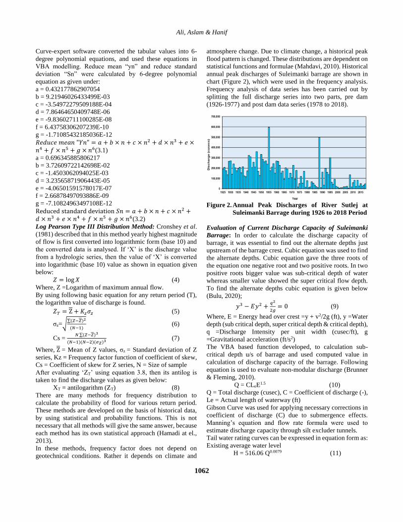
atmosphere change. Due to climate change, a historical peak

flood pattern is changed. These distributions are dependent on

statistical functions and formulae (Mahdavi, 2010). Historical

annual peak discharges of Suleimanki barrage are shown in

chart (Figure 2), which were used in the frequency analysis.

Frequency analysis of data series has been carried out by

splitting the full discharge series into two parts, pre dam

(1926-1977) and post dam data series (1978 to 2018).

Figure 2. Annual Peak Discharges of River Sutlej at

Suleimanki Barrage during 1926 to 2018 Period

Evaluation of Current Discharge Capacity of Suleimanki

Barrage: In order to calculate the discharge capacity of

barrage, it was essential to find out the alternate depths just

upstream of the barrage crest. Cubic equation was used to find

the alternate depths. Cubic equation gave the three roots of

the equation one negative root and two positive roots. In two

positive roots bigger value was sub-critical depth of water

whereas smaller value showed the super critical flow depth.

To find the alternate depths cubic equation is given below

(Bulu, 2020);

𝑦3 − 𝐸𝑦2 +𝑞2

2𝑔= 0 (9)

Where, E = Energy head over crest =y + v2/2g (ft), y =Water

depth (sub critical depth, super critical depth & critical depth),

q =Discharge Intensity per unit width (cusec/ft), g

=Gravitational acceleration (ft/s2)

The VBA based function developed, to calculation sub-

critical depth u/s of barrage and used computed value in

calculation of discharge capacity of the barrage. Following

equation is used to evaluate non-modular discharge (Brunner

& Fleming, 2010).

Q = CLeE1.5 (10)

Q = Total discharge (cusec), C = Coefficient of discharge (-),

Le = Actual length of waterway (ft)

Gibson Curve was used for applying necessary corrections in

coefficient of discharge (C) due to submergence effects.

Manning’s equation and flow rate formula were used to

estimate discharge capacity through silt excluder tunnels.

Tail water rating curves can be expressed in equation form as:

Existing average water level

H = 516.06 Q0.0079 (11)

Flood Evaluation and management by VBA model for Hydraulic Structures

1063

Equation no. 11 used to calculate the tail water level (Nespak,

2012). Discharging capacities of the various tunnels of silt

excluder have been calculated after making due allowance for

the head losses inside the tunnels as mentioned by USBR

(1987) and Chow (1988), following head losses alongwith

their loss coefficients were considers and used to provide

allowance for head losses inside the tunnels:

i. Entrance Loss ………With a loss coefficient of 0.7

ii. Contraction Loss …...With a loss coefficient of 0.3

iii. Exit Loss ……………With a loss coefficient of 1.0

iv. Friction Loss ………..With Manning’s equation with ‘n’

value of 0.018

After determining the 100-year flood discharge at barrage,

checked the barrage capacity by fixing Total Energy Level

(TEL) with respect to guide banks levels and then calculated

the hydraulic jump elevation. According to Garg (2005)

hydraulic jump should be at the toe of the d/s glacis of the

hydraulic structure. Hydraulic jump should not sweep from

the toe of the d/s glacis. In the present research the VB

function was developed using the conjugate depth methods

for calculate the hydraulic jump, with 10 % submergence in

Tail water level (Garg, 2005). Also use criteria given by

Peterka (1984), “Hydraulic Design of Stilling Basins and

Energy Dissipaters” (Peterka, 1984).

Evaluation of Flood Management Structural Interventions:

The existing barrage capacity was inadequate to pass design

flood for 100-year return period. The following four

interventions were evaluated to manage estimated flood

design discharge:

(1) Enhancing barrage capacity by raising high flood level

(HFL):

i. Raising emergency HFL by 1.5 ft

ii. Raising emergency HFL by 1.94 ft

iii. Raising emergency HFL by 2 ft

(2) Enhancing barrage capacity by lowering barrage crest

and raising HFL

(3) Enhancing barrage capacity by addition of bays and

raising HFL

(4) Construction of bypass weir and raising HFL of barrage

RESULTS AND DISCUSSION

Flood Peak Discharge Analysing Combined Pre- and Post-

dam Data Series of 1926 to 2018 Period: In this series, data

of 93 years was used to estimate flood for different return

periods. In Pakistan, 100-year return period is generally used

in the design of barrages and small dams or small hydraulic

structures. In this series, barrage faced only two time an

exceptionally high flood first in year 1955 and second in 1988.

The frequency analysis of combined pre-and post-dam series

for period of 1926 to 2018 carried out by EV-I and LP-III

distributions. The results of this analysis are presented in

Table 2 and Figure 3.

Table 2. Results of Frequency Analysis Using Combined

Pre- &Post-dam Data of 1926 to 2018 Period.

Return Period EV-I (Cusec) LP-III (Cusec)

2 127,081 108,408.7

10 300,235 341,990.5

25 387,385 463,569.6

50 452,038 548,221.5

100 516,214 625,898.0

200 580,156 696,663.0

1000 728,721 848,971.8

Figure 3. Flood Frequency Analysis for Combined Pre-

and Post-dam Data of 1926 to 2018 Period.

The results showed that flood peaks even for the lower return

periods are quite high. The 100-year return period flood

discharges determined by EV-I and LP-III were 516,214 and

625,898 cusec, respectively. It reflected that LP-III estimated

21 % higher flood discharge compared to that determined by

EV-I method. Based on regression analysis, trend line value

of R-square (R2) was 0.9668 for Gumbel (EV-I) distribution

while R2 value for LP-III distribution was 0.9973. It shows

that LP-III is good fit of line to data, because its R2 value is

close to 1 as compared to EV-1 value.

Flood Peak Discharge Analysing Pre-dam Data Series of

1926 to 1977 Period: The results of frequency analysis of pre-

dam data series of 1926 to 1977 period performed using EV-

I and LP-III distribution methods are presented in Table 3 and

Figure 4. For this discharge data series, flood peaks calculated

by EV-I distribution for different return periods were quite

high compared to those calculated by LP-III distribution. For

example, for 100-year return period, estimated flood

discharge value by EV-I distribution was 519,029 cusec

whereas same value determined by LP-III method was

355,061 cusec reflecting Gumbel’s estimate 46% higher than

that of LP-III.

These results revealed that flood peaks estimated by LP-III

distributions do not vary after 10 year to 1000 year return

periods which is not reliable and acceptable due to an error in

prediction of flood for 1926-1977 series. Therefore, this

method is not appropriate for this discharge series due to

unrealistic results. This reflects that Gumbel method is more

appropriate for Pakistani conditions. Whereas, based on

regression analysis, trend line value of R-square (R2) for

Ali, Aslam & Hanif

1064

Gumbel (EV-I) distribution was 0.9692 while R2value for LP-

III distribution was 0.8652. It presents that Gumbel (EV-1) is

good fit of line to data because its R2 value is close to 1.

Table 3. Results of Frequency Analysis Using Pre-dam

Data of 1926 to 1977Period

Return Period EV-I (Cusec) LP-III (Cusec)

2 185,211 205,088

10 333,751 303,059

25 408,513 321,987

50 463,975 330,126

100 519,029 335,061

200 573,881 338,185

1000 700,942 348,993

Figure 4. Flood Frequency Analysis for Pre-dam Data of

1926 to 1977 Period

Flood Peak Discharge Analysing Post-dam Data Series of

1978 to 2018 Period: The observed peak flood discharge in

1988 (post-dam scenario) at Suleimanki barrage was 499,000

cusec. The results of frequency analysis of post-dam

discharge data series for period of 1978 to 2018performed

using EV-I and LP-III methods are presented in Table 4 and

Figure 5. For 100-year return period, EV-I flood discharge

estimation was 384,765 cusec compared to 626,572 cusec

computed by LP-III reflecting 63% higher flood discharge

than EV-I value. Table 4 presents a comparison of flood peak

discharges estimated by EV-I and LP-III methods for

discharge data series. Trend line value of R-square (R2) for

Gumbel (EV-I) distribution was 0.9692 while R2 value for LP-

III distribution was 0.8652. It presents that Gumbel (EV-1) is

good fit of line to data.

Table 4. Results of Frequency Analysis Using Post-dam

Data of 1978 to 2018Period.

Sr # Return Period EV-I (Cusec) LP-III (cusec)

1 2 56,521 36,430

2 10 202,580 164,870

3 25 276,094 296,896

4 50 330,631 438,221

5 100 384,765 626,572

6 200 438,701 874,136

7 1000 563,640 1,773,968

Figure 5. Flood Frequency Analysis for Post-dam Data of

1978 to 2018 Period.

The results reveal that the upstream dams in India have

significant effect on flood peaks at Suleimanki barrage

therefore, water flow in River Sutlej have been changed and

for flood evaluation in present condition at Suleimanki

barrage, post-dam series was most suitable condition.

In post-dam series, it showed that peak floods for low return

period have been reduced at Suleimanki barrage but for high

return period there is still chance to face a high flood at

barrage. Design return period of 100 year is considered

satisfactory for fixing design flood values for barrages in

Pakistan. For 100-year return period Gumbel distribution

estimated the flood peak discharge of 384,765 cusec. The

Gumbel (EV-I) R2 value for post-dam series is 0.971 while

LP-III R2 value is 0.9335 showing that Gumbel (EV-1) is

good fit of line to data and Gumbel (EV-1) distribution is

reliable for predicting expected flow in the river for 100 year

return period.

Table 5. Comparison of 100 Year Return Period Flood

Peak Discharges Determined by EV-I and LP-III

Methods for Three discharge Data Series

Sr.# Discharge Data Series EV-I

(Cusec)

LP-III

(Cusec)

1 Combined pre-and post-dam

series:1926 to 2018

516,214 625,898

2 Pre-dam series: 1926 to 1977 519,029 335,061

3 Post-dam series: 1978 to 2018 384,765 626,572

Table 6. Comparison of trend line R-square values by EV-

I and LP-III Methods

Sr. Discharge Data Series Gumbel

(EV-1)

R2 Value

Log

Pearson

R2 value

1 Combined pre-and post-dam

series:1926 to 2018

0.9668 0.9973

2 Pre-dam series: 1926 to 1977 0.9692 0.8652

3 Post-dam series: 1978 to 2018 0.9710 0.9335

Trend line R2 (R-square) values for Gumbel (EV-1) and LP-

III distributions have been depicted in Table 5. A trend line is

most reliable when its R-squared value is at or close to 1.

Flood Evaluation and management by VBA model for Hydraulic Structures

1065

Therefore, R-square values indicates that LP-III distribution

is suitable for combined pre-& post-dam series (1926-2018)

whereas Gumbel (EV-1) distribution is relatively more good

fit of the line to the data for pre-dam (1926-1977) & post dam

series (1977-2018).

Comparison of results with Previous Study: Feasibility study

of Suleimanki Barrage has been carried out by Nespak in

November, 2012, the frequency analysis has been carried by

only Gumbel (EV-1) for discharge series of 84 years (1925-

2008). Estimated flood peak discharge for 100-year return

period, was 449,000 cusec for the pre-dam and 416,000 cusec

for the post-dam conditions [14]. It is necessary to mention

that the present condition of barrage has been changed, it has

silt excluder in left pocket and its stilling basin level have

been raised by 0.75 ft. Therefore, it was necessary to re-

evaluate its flood discharge for 100-year return period by

taking into account the latest riverine discharge data up to

2018 (93-year discharge series).

In present research updated discharge series of 93 years

(1926-2018) is used. Developed a VBA based computer

model to compare the two distributions methods Gumbel

(EV-1) and LP-III along with R2 value and found that LP-III

distribution is appropriate only for combined pre & post dam

scenario having long discharge series (1926-2018). However,

Gumbel (EV-1) distribution is more accurate for post dam

scenario having shorter discharge series. Estimated flood

peak discharge for 100-year return period, by Gumbel (EV-1)

is 384,765 cusec, 8% lower than the feasibility study

estimated discharge. The continues reduction in discharge

peaks have significant impact on estimated flood peaks.

Similarly, flood management interventions accordingly need

to decide.

Evaluation of Current Discharge Capacity of Suleimanki

Barrage: In 1926, barrage was designed for 325,000 cusec

with upstream HFL of 572.00 ft and downstream HFL of

569.00 ft. The main weir share was taken as 210,000 cusec

and each under sluice was taken as 57,500 cusec. The

coefficient of discharge for weir portion was considered as

3.10 and for under sluices 2.5 based on the submergence

conditions of 75 % in main weir portion and 85 % in under

sluice portion, respectively.

But, during evaluation of discharge capacity of barrage in its

present condition (2017), it was observed that now it has flood

passing capacity of 295,492cusec, water level downstream of

the barrage had been raised due to phenomena of accretion at

downstream of barrage. It directly affected the submergence

conditions of barrage. The submergence was 80% in main

weir portion and was 88% in under sluice portion.

Consequently, hydraulics of barrage was changed. The

submergence directly affects the coefficient of discharge. The

VBA worksheet model revealed that the coefficient of

discharge for weir portion was 2.95 and 2.5 for undersluices

(Sharma, 2017). The VBA model found that to restore the

original design capacity of barrage (325,000 cusec), HFL

needs to be raised by 0.66 ft as shown in Table 7.

Table 7. Current Discharge Capacity of Suleimanki

Barrage

Sr. Raise in high flood

level (ft)

High flood

level (HFL) (ft)

Total discharge

(Cusec)

1 0 (Present

condition)

572.00 295,492

2 0.66 572.66 3,25,000

Evaluation of Structural Flood Management Interventions

Intervention 1: Enhancing Discharge Capacity by Raising

HFL: Safe discharge capacity for the barrage is the peak flood

discharge which can be passed through the barrage with

adequate (10%) hydraulic jump submergence. The evaluation

of the intervention; raising HFL through VBA model

revealed that entire high flood could be passed through the

existing barrage resulting in higher flood level as compared

to the design value. This situation gives rise to a potential

danger of breaches through marginal bunds due to increased

hydraulic pressures. Also, the quantity of flood discharge,

passing per unit width of the barrage, gets enhanced. This may

result in damages to different components of the barrage, like

marginal bunds, guide bunds, spurs. Therefore, these

components need to be raised and strengthened under modern

design criteria. Other components like, stilling basin length

and flexible stone apron were calculated by VBA model and

it was found that just increasing the length of stone apron

needs to be increased. The evaluation results of options of 1.5,

1.94 and 2 ft raise in original HFL of 572 ft are presented in

Table 8 and Figure 6.

Table 8. Evaluation Results of Enhancing Barrage

Capacity by Raising HFL Intervention.

Sr. Raise in HFL (ft) HFL (ft) Total discharge (cusec)

1 0 (Present

condition)

572.00 295,492

2 1.50 573.50 3,64,510

3 1.94 573.94 3,85,000

4 2.00 574.00 3,88,351

Figure 6. Evaluation Results of Enhancing Barrage

Capacity by Raising HFL Intervention

Ali, Aslam & Hanif

1066

Table 9. VBA model

Intervention 2: Enhancing Barrage Capacity by Lowering

Barrage Crest and Raising HFL: The evaluation of the

intervention; lowering crest of weir, by breaking the main

weir crest the severe flood discharge could be passed through

the existing barrage, but it was found that there is also a need

to raise the HFL (Table 10). In under sluice portion crest can’t

be lowered because it is already at the level of upstream floor,

therefore, this intervention will be applied only to main weir.

But, this intervention has a major demerit for the modification

process. Piers and the weir crest floors are two independent

structural elements of two different materials. Breaking and

lowering of crest, can cause cracks in the concrete masonry

which cannot be ignored, this shall eventually create problems

for the barrage structure. Consequently, this intervention was

not considered feasible for adoption for flood management.

Table 10. Sr. Crest Level

Lowered by

1.0 ft (ft)

HFL (ft) Table 10. Evaluation

Results of Enhancing Barrage

Capacity by Lowering Barrage

Crest by 1.0 ft and Raising HFL

by 1.5 ft Intervention

Total

Discharge

(Cusecs)

1 559 572 without increase 3,09,698

2 559 573.5 with 1.5 ft increase 3,85,000

Intervention 3: Enhancing Barrage Capacity by Addition of

Bays and Raising HFL: Evaluation of intervention; addition

of bays, revealed that by increasing the number of bays on the

right undersluice of barrage, danger of greater pressure on

different embankments of barrage could be eliminated. For

this purpose, the head regulator of Pakpattan canal will have

to be dismantled and reconstructed at new location in the

relocated right abutment wall. Upstream and downstream

guide banks along the right side of the barrage would have to

be dismantled and reconstructed at the extended end of the

barrage. During low discharges, there is a tendency of bela

and island formation upstream of the barrage. Widening of

waterway is likely to accentuate this problem. Vigilant

regulation and proper river training will be required to tackle

such problems, which is common at almost all barrages to

varying degrees. This alternative is not viable; therefore, this

intervention was also not considered for enhancing barrage

capacity. The evaluation results of this intervention are

depicted in Table 11.

Table 11. Evaluation Results of Enhancing Barrage

Capacity by Addition of Bays and raising HFL

Intervention

Sr. Parameters Results

1 Discharge 89,273 cusec

2 Right undersluice one bay

discharge

6926 cusec (At HFL

572.00 ft)

3 Number of additional bays 13

4 Width of each bay 30 ft

5 Clear waterway 390 ft

6 Number of piers 12

7 Width of each pier 5 ft

8 Total width of extended portion 450 ft

Intervention 4: Construction of Bypass Weir and Raising

HFL of Barrage: The intervention; construction of bypass

weir, can be applied for management of flood for more than

100-year return period. Barrage has faced more than 1:100

year return period discharge. Under this scenario, provision

of bypass channel with auxiliary weir is best option. Barrage

can pass 388,000 cusec at HFL 574.00. Therefore, the only

option to pass more than 1:100-year return period discharge,

is to provide bypass canal with auxiliary head regulator at its

right side. Proper arrangements will also be needed for level

crossing/aqueduct or syphon at Pakpattan canal upper for

crossing of bypass channel having capacity more than 89,273

cusec. For 100-year return period, this intervention is not

recommended, but for more than 100-year return period or for

1988 flood value this intervention is best one. The evaluation

results of this intervention are provided in Table 12.

Finally, the intervention; raising HFL by 1.94 ft can be

considered as the most suitable intervention to pass the

adopted design flood of 384,765 cusec.

Flood Evaluation and management by VBA model for Hydraulic Structures

1067

Table 12. Evaluation Results of Construction of Bypass

Weir and raising HFL of Barrage Intervention

Sr. Parameters Results

1 Discharge 89,273 cusec

2 Right undersluice one bay

discharge

6926 cusec (At HFL

572.00 ft)

3 Number of additional bays 18

4 Width of each bay 40 ft

5 Clear waterway 720 ft

6 Number of piers 17

7 Width of each pier 5 ft

8 Total width of extended portion 805 ft

Conclusions and Recommendations: It is concluded that

dams on River Sutluj have significant effect on flood peaks at

Suleimanki barrage, water flow behaviour in River Sutlej has

been changed for flood evaluation in present condition at

Suleimanki barrage. Based on regression analysis, LP-III

distribution is suitable for only combined pre-& post-dam

series (1926-2018). Whereas, Gumbel’s distribution (EV-I)

trend line R2 value is good fit of line to data in pre-dam

scenario (1947 to 1977) & post dam scenario (1978-2018).

Post-dam scenario was considered as the design (peak) flood

discharge for the barrage for 100 year return period and find

that it R2 value is good fit of line to data. Therefore, Gumbel

(EV-1) distribution method is more suitable for predicting

expected flood flow in the river Sutlej for 100 year return

period.Moreover, Gumbel’s distribution (EV-I) results

illustrates that flood peaks for the lower return periods are

reduced significantly due to the construction of Indian dams

on River Sutlej while for the higher return periods the

reduction in flood peak is much smaller. The design flood

discharge 384,765 cusec computed by EV-I method for

1:100-year return period. Whereas, current discharge capacity

of barrage to pass the flood came out about 295,492 cusec.

Evaluation of different flood management structural

interventions revealed that Suleimanki barrage can pass the

1:100-year flood discharge of 384,765 cusec byraising HFL

(1.94 ft) without any modification in the existing structure.

Accordingly, upstream embankments may be upgraded with

enough free board. The implementation of management

techniques emerged from the proposed research could prevent

flood damages in future. Developed model is also applicable

to other barrages / hydraulic structures for estimation and

management of flood.

Recommendations: Though the HFL computed by using

computer model is quite accurate however, it is recommended

that before applying recommended proposal practically,

physical model study should be conducted. The prediction

curves in EV-I and LP-III methods should be modified to

obtain more accurate results especially when large series of

historical floods are available.

There were limitations in developed model regarding

economic analysis therefore, for structural flood management

interventions economic analysis need to develop.

REFERENCES

Abida, H., E Manel. 2007. Probability distribution of flood

flow in Tunisia. J. Hydr. Sys. Sci. 4: 957-981.

Akhtar, A. 2013. Indus Basin Floods Mechanisms, Impacts,

and Management, Asian Development Bank. Manila,

Philippines.

Annual Administration Report (AAR). 1999. Bakhra Beas

Management Bord, New Dehli, India.

Asian Development Bank. 2017. Indus Basin Floods

Mechanisms Impacts and Management, Manila,

Philippines.

Brunner, G.W and M.J. Fleming, 2010. U.S. Army Corps of

Engineers, Hydrology Engineering Centre, HEC-RAS

4.1-2010, California, USA.

Bulu, A. Dr. 2020. Specific Energy and Hydraulic Jump. Ist.

Tec. Uni, Civ. Eng. Dep. Hydr. Div. Hyd. Div, Istanbul,

Turkey.

Chow, T.V. 2009. Open Channel Hydraulics, International

Student Edition, McGraw-Hill, London, New York.

Cronshey, R., H.G. Rallison., F.J. Miller and W.D. Newton.

1981. Guideline for determining flood flow frequency,

U.S Department of the Interior Bullitien17, United

States.

Federal Flood Commission (FFC). 2016. Annual Flood

Report, Ministry of Water & Power, Govt of Pakistan,

Islamabad, Pakistan.

Flood Fighting Plan (FFP) of Suleimanki Barrage. 2013.

Punjab Irrigation Department (PID). Ministry of

Irrigation, Govt of Punjab, Pakistan.

Garg, S.K. 2005. Irrigation Engineering & Hydraulic

Structure, 19th Revised Ed. New Delhi, India.

Green, J., S. Bullen, R. Bovey and A. Michael., 2007. VBA

Programmer’s Reference, 1st Ed. Toronto, Canada.

Hamadi, K., A. Samaneh, and N. Zohrabi. 2013. Frequency

analysis of low-flow in the large Karoun river basin in

Iran. J. Appl Bas. Sci. pp:148-151.

Harter, L.H. 2007. Another look at plotting positions, j.

Comm. Stat. pp.1613-1633.

Kaw, K.A., E.K. Kalu and D. Nguyen., 2011. Numerical

Methods with Applications, 2nd Ed. New Mexico, USA.

Kjeldsen, T. R., J. C. Smithers and R. E. Schulze. 2001.

Regional flood frequency analysis in the Kwazulu-natal,

South Africa, using the index-flood method. J. Hydro.

255:194-211.

Kot, L. & S. Nadarajah. 2000., Extreme value distribution

theory and applications, London, UK.

Mahdavi, M., 2010. Determining suitable probability

distribution models for annual precipitation data. J. Sust.

Devel. Vol 3, pp. 159:164.

Ali, Aslam & Hanif

1068

Naseer, M. 2010-2012. Malevolent Floods of Pakistan,

Strengthening Participatory Organization, Islamabad,

Pakistan.

NESPAK. 2012. Punjab Irrigated Agriculture Investment

Program (PIAIP), Feasibility Study of Suleimanki

Barrage, Vol. I-II, Irrigation Department, Govt. of

Punjab, Lahore, Pakistan.

Nirman, B. 2017. Flood frequency analysis using Gumbel's

distribution method: A case Study of Lower Mahi Basin,

India. J. of Wat. Res. Sci. 6:51-54.

Peterka, A.J. 1984. Hydraulic Design of Stilling Basins and

Energy Dissipaters, 8th Ed. United States, America.

Ren, M., X. He, G. Kan, F. Wang, H. Zhang, H. Li and Z.

Zhang., 2017. A comparison of flood control standards

for reservoir engineering for different countries. J. Wat 9,

152.

Sajid I. 2011. Rehabilitation of Islam Barrage for the safe

passage of design flood. Msc. Dep. Civ. Eng, Uni. Eng.

Tech,. Lahore, Pakistan.

Sharma, S.K. 2017. Irrigation Engineering and Hydraulic

Structures, 3rd revised Ed. New Delhi, India.

Sun, P., W. Qingzhi, Z. Qiang, S.P. Vijay, S. Yuyan, L.

Jianfeng. 2018, Nonstationary evaluation of flood

frequency and flood risk in the Huai River basin, China.

J. Hydr. V. 567, pp. 393-404.

Subramanya, K. 2009. Flow in Open Channels, 3rd Ed.

McGraw-Hill, New Delhi, India.

US Army Corps of Engineers. 1993. Hydrologic Frequency

Analysis, 1st Ed. Washington, D.C. USA.

USBR, 1987. Design of Small Dams 3rd Ed. United States,

America.

Vogel, M.R. and W. Ian. 1996. Probability distribution of

annual maximum, mean & minimum stream flows in the

United States. J. Hyd. Eng. 12:69-76.

Wu, S.J., J.C.Yang and Y.K.Tung., 2011. Risk Analysis for

Flood Control Structure Under Consideration of

Uncertainties in Design Flood. J. Natu. Haz. 58:117–140.

[Received 27 Nov 2019; Accepted 29 Oct. 2020; Published

(online) 25 Jun 2021]