Development and Application of a Logistic-Based Systolic ...

ORIGINAL PAPER

Development and Application of a Logistic-Based Systolic Modelfor Hemodynamic Measurements Using the Esophageal DopplerMonitor

Glen M. Atlas

� Springer Science+Business Media, LLC 2008

Abstract The esophageal Doppler monitor (EDM) is a

clinically useful device for minimally invasive assessment

of cardiac output, preload, afterload, and contractility. An

empirical model, based upon the logistic function, has been

developed. Use of this model illustrates how the EDM could

estimate the net effect of aortic and non-aortic contributions

to inertia, resistance, and elastance within real time. This is

based on an assumed mechanical impedance conceptually

resembling that of a series arrangement of a spring, mass,

and dashpot. In addition, when used with an invasive radial

arterial catheter, the EDM may also estimate aortic pulse

wave velocity, as well as aortic characteristic impedance,

and characteristic volume. Approximations of left ventric-

ular stroke work and stroke power can also be made.

Furthermore, the effects of inertia, resistance, and elastance,

on mean blood pressure during systole, can be quantified.

These additional parameters could offer insight for clini-

cians, as well as researchers, and may be beneficial in

further examining and utilizing clinical hemodynamics with

the EDM. These additional measurements also underscore

the need to integrate the EDM with existing and future

monitoring equipment.

Keywords Esophageal doppler � Hemodynamic model �Logistic

Introduction

The esophageal Doppler monitor (EDM) offers clinicians,

both rapid and safe cardiovascular assessment in real time.

Historically, evaluation of hemodynamic parameters has

been commonly done with a pulmonary artery occlusion

[Swan-Ganz] catheter. These catheters are highly invasive

and fraught with potential life-threatening complications

(Domino et al. 2004; Vincent et al. 1998) which are sum-

marized in Table 1 (American Society of Anesthesiologists

Task Force on Guidelines for Pulmonary Artery 2003).

Additionally, the accuracy of the data, derived from these

catheters, can be flawed by coexisting diseases, misinter-

pretation, and other conditions (American Society of

Anesthesiologists Task Force on Guidelines for Pulmonary

Artery 2003; Rothenberg and Tuman 2000). Furthermore,

in spite of the tremendous risks associated with the

pulmonary artery occlusion catheter, no significant benefit

from these devices has been conclusively and consistently

demonstrated through multiple large-scale patient-based

outcome studies (American Society of Anesthesiologists

Task Force on Guidelines for Pulmonary Artery 2003;

Polanczyk et al. 2001; Warzawski and Deye 2003; Sand-

ham and Hull 2003; The National Heart, Lung, and Blood

ARDS Clinical Trials Network 2006).

Transesophageal echocardiography (TEE) can also be

used to assess hemodynamic status. However, this requires

expensive technology as well as some significant training.

Furthermore, the TEE probe is considerably larger than

those probes associated with the EDM.

G. M. Atlas (&)

Department of Anesthesiology, University of Medicine

and Dentistry of New Jersey, New Jersey Medical School,

Newark, NJ, USA

e-mail: [email protected]

G. M. Atlas

Department of Chemistry, Chemical Biology & Biomedical

Engineering, Stevens Institute of Technology, Hoboken, NJ,

USA

G. M. Atlas

Department of Biomedical Engineering, Rutgers University,

Piscataway, NJ, USA

123

Cardiovasc Eng

DOI 10.1007/s10558-008-9057-9

The major advantage of TEE, over other devices, is its

ability, using imaging, to visualize and assess cardiac

anatomy and associated dynamic wall and valvular changes

(Vignon 2005). However, TEE can only be used on an

intermittent basis. This is due to the large size of its probe.

Whereas the EDM, with its significantly smaller probe, can

be used for an extended period of time (English and

Moppett 2005). It should be noted that the EDM measures

only distal aortic blood flow velocity.

With the EDM, preload can be assessed by examination of

corrected flow time, FTc (Singer and Bennett 1991; DiCorte

et al. 2000; Feldman et al. 2004; Seoudi et al. 2003; Gan

et al. 2002). Clinically, FTc correlates with preload as

measured with a pulmonary artery occlusion [Swan-Ganz]

catheter (Madan et al. 1999). The relationship between flow

time (FT) and FTc is based upon heart rate (HR) in beats per

minute: FT ¼ FTcffiffiffiffiffiffiffiffiffiffiffiffiffiffi

60=HRp

where FT represents left ven-

tricle ejection time during systole. This is illustrated in Fig. 1.

In addition, FTc has been shown to correlate better with

left ventricular (LV) end-diastolic area than pulmonary

artery occlusion pressure (DiCorte et al. 2000). Stroke

volume (SV), as measured with the EDM, can also be used

to assess preload (Roeck et al. 2003). However, changes in

contractility and flow time have to taken into account when

using this parameter (Kumar et al. 2004) (See Appendix

A). Furthermore, it appears that low stroke volume, when

measured with an EDM, may also have prognostic value

following cardiac surgery (Poeze et al. 1999).

With the EDM, contractility is readily quantified by

examining peak velocity and acceleration of distal aortic

blood flow. In addition, that portion of cardiac output (CO),

which is measured in the distal aorta, is continuously

assessed by determining the product of distal aortic diam-

eter and the velocity of descending aortic blood flow. A

correction, based upon a linear regression, of the blood

flow in the distal aorta, is then used to determine total

cardiac output (See Appendix A) (Boulnois and Pechoux

2000; Dark and Singer 2004; Valtier et al. 1998; Lafan-

echere et al. 2006).

Furthermore, distal aortic diameter can be directly

measured using an M-mode function such as that available

on the Arrow Hemosonic� EDM. This feature also helps to

focus the ultrasound directly on the aorta thus assuring that

the angle of the Doppler signal is correct. Consequently,

diameter and velocity are accurately and continuously

assessed (Boulnois and Pechoux 2000).

Afterload can also be clinically measured with the

EDM. This is accomplished by calculating: TSVR ¼MAP=CO where TSVR represents aortic characteristic

resistance. MAP is mean arterial blood pressure which can

be measured either noninvasively, with a blood pressure

cuff, or invasively with an indwelling arterial catheter and

transducer. Typically, the clinician will input the mean

arterial pressure into the EDM. Following this, the EDM

will then calculate TSVR.

Central venous pressure (CVP), if available, can also be

used to calculate SVR using the same formula as a one

would use with a pulmonary artery occlusion or CVP

catheter: SVR ¼ MAP�CVPCO

:

The EDM is typically placed orally in anesthetized

patients whose trachea is intubated. Nasal placement, in

awake patients, has also been described. This represents a

distinct advantage of the EDM over TEE (English and

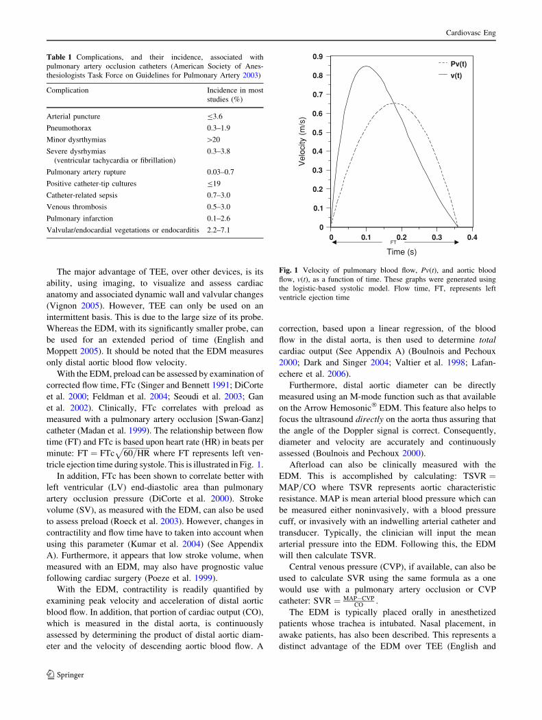
Table 1 Complications, and their incidence, associated with

pulmonary artery occlusion catheters (American Society of Anes-

thesiologists Task Force on Guidelines for Pulmonary Artery 2003)

Complication Incidence in most

studies (%)

Arterial puncture B3.6

Pneumothorax 0.3–1.9

Minor dysrthymias [20

Severe dysrhymias

(ventricular tachycardia or fibrillation)

0.3–3.8

Pulmonary artery rupture 0.03–0.7

Positive catheter-tip cultures B19

Catheter-related sepsis 0.7–3.0

Venous thrombosis 0.5–3.0

Pulmonary infarction 0.1–2.6

Valvular/endocardial vegetations or endocarditis 2.2–7.10.20.10 0.3 0.4

Time (s)

0

0.1

0.2

0.3

0.4

0.5

0.6

0.7

0.8

0.9

Vel

ocity

(m/s

)

Pv(t)

v(t)

FT

Fig. 1 Velocity of pulmonary blood flow, Pv(t), and aortic blood

flow, v(t), as a function of time. These graphs were generated using

the logistic-based systolic model. Flow time, FT, represents left

ventricle ejection time

Cardiovasc Eng

123

Moppett 2005; Atlas and Mort 2001; Levy 2001; Dodd

2002).

This paper examines additional ‘‘new’’ measurements

with the EDM. These include hemodynamic assessments of

inertia, resistance, and elastance conceptually resembling

a net series arrangement of a spring, mass, and dashpot

(Nichols and O’Rourke 2005). To exemplify this, a logis-

tic-based systolic model is developed and applied to distal

aortic blood flow. Means of estimating aortic pulse wave

velocity, as well as aortic elastance, characteristic volume,

and characteristic impedance are also examined. Further-

more, evaluations of both left ventricular stroke work and

stroke power can be made. Also, the individual effects, of

inertia, resistance, and elastance, on mean blood pressure

during systole, can be assessed. These additional mea-

surements depend upon the EDM ultimately being

integrated with existing OR and ICU monitors.

Development of a Logistic-Based Systolic Model

Pulmonary Circulation and Flow Time

By using a model whose form is similar to the logistic

function (Beltrami 1987), Pv(t), the velocity of pulmonary

artery blood flow, can be represented as a parabola-like

function occuring over the course of ventricular ejection

time or flow time:

PvðtÞ ¼ a 1� t

FT

� �

th i

: 0� t� FT ð1Þ

where a is an acceleration term with a value of about

7.25 m s-2. Clinically, in humans with normal cardiac

function, the velocity of pulmonary artery blood flow has

been observed to be age-independent (Gardin et al. 1987).

A plot of Pv(t) is shown in Fig. 1.

FT represents flow time, during systole, or left ventricle

ejection time. Corrected flow time, FTc, has a normal range

of 330–360 and is ‘‘expressed’’ in terms of milliseconds. In

addition, FT is age-independent whereas FTc increases

with age (Gardin et al. 1987).

For computational purposes, both left and right ven-

tricular ejection times (flow time or FT) are assumed to be

equal. In addition, this model is only applicable during

systole: 0 B t B FT.

It should be noted that the EDM does not directly

measure right heart function. However, changes in right

heart function may ultimately be detected as changes in the

velocity of distal aortic blood flow.

In this model, displacement, as a function of time, also

maintains the familiar logistic sigmoid character (See

Appendix B). Logistic-based modeling has also been used

in other cardiovascular settings (Matsubara et al. 1995).

Systemic Circulation

Equation (1), for pulmonary artery velocity, can be modi-

fied to accommodate the ‘‘pumping effects’’ of the left

ventricle:

vðtÞ ¼ abe�ct 1� t

FT

� �

th i

: 0� t� FT ð2Þ

where v(t) represents the velocity of distal aortic blood

flow. The peak value for distal aortic blood flow velocity

has been shown to have an age-dependent normal range

(Mowat et al. 1983).

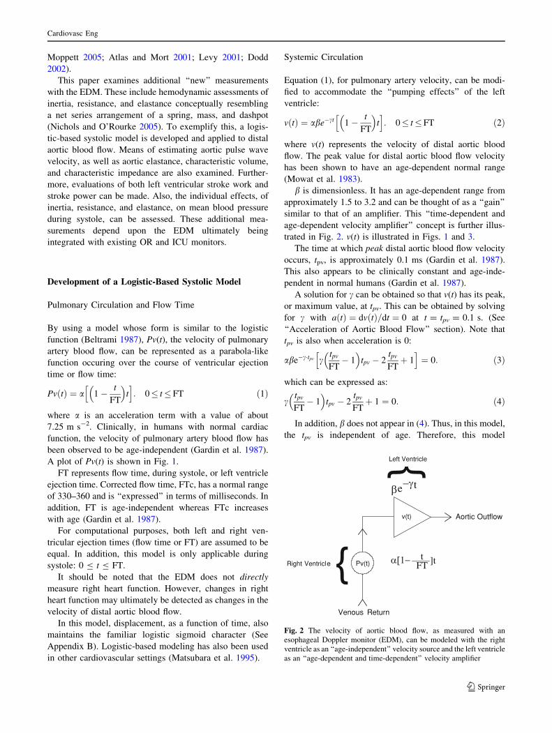
b is dimensionless. It has an age-dependent range from

approximately 1.5 to 3.2 and can be thought of as a ‘‘gain’’

similar to that of an amplifier. This ‘‘time-dependent and

age-dependent velocity amplifier’’ concept is further illus-

trated in Fig. 2. v(t) is illustrated in Figs. 1 and 3.

The time at which peak distal aortic blood flow velocity

occurs, tpv, is approximately 0.1 ms (Gardin et al. 1987).

This also appears to be clinically constant and age-inde-

pendent in normal humans (Gardin et al. 1987).

A solution for c can be obtained so that v(t) has its peak,

or maximum value, at tpv. This can be obtained by solving

for c with aðtÞ ¼ dvðtÞ=dt ¼ 0 at t = tpv = 0.1 s. (See

‘‘Acceleration of Aortic Blood Flow’’ section). Note that

tpv is also when acceleration is 0:

abe�c�tpv ctpv

FT� 1

� �

tpv � 2tpv

FTþ 1

h i

¼ 0: ð3Þ

which can be expressed as:

ctpv

FT� 1

� �

tpv � 2tpv

FTþ 1 ¼ 0: ð4Þ

In addition, b does not appear in (4). Thus, in this model,

the tpv is independent of age. Therefore, this model

t ]tFT

e t

Aortic Outflow

Venous Return

Left Ventricle

Right Ventricle Pv(t)

v(t)

Fig. 2 The velocity of aortic blood flow, as measured with an

esophageal Doppler monitor (EDM), can be modeled with the right

ventricle as an ‘‘age-independent’’ velocity source and the left ventricle

as an ‘‘age-dependent and time-dependent’’ velocity amplifier

Cardiovasc Eng

123

maintains age-independence for time to peak velocity. It

should also be noted that a does not appear in the above

formula and that tpv, in the distal aorta, can be modeled

independently of pulmonary artery blood flow.

Solving (4) for c yields:

c ¼2� FT

tpv

tpv � FT: ð5Þ

c is then calculated as 6.154 s-1. This is based on tpv = 0.1

and a FT = 360 ms.

Clinically, a reduction in left ventricular contractility

can be observed as a greater tpv as well as a decrease in

acceleration and/or peak velocity (DuBourg et al. 1993,

Wallmeyer et al. 1986). With this model, an increase in tpv

is observed as a decrease in the value of c:

limtpv!FT

2

c ¼ limtpv!FT

2

2� FTtpv

tpv � FT¼ 0: ð6Þ

Acceleration of Distal Aortic Blood Flow

Acceleration of distal aortic blood flow is also clinically

useful in assessing left ventricular contractility (DuBourg

et al. 1993) and is readily determined with the EDM. It can

be modeled by differentiating (2) with respect to time:

dvðtÞdt¼ aðtÞ ¼ abe�ct c

t

FT� 1

� �

t � 2t

FTþ 1

h i

: ð7Þ

Age-dependent normal values, for acceleration of distal

aortic blood flow, have also been clinically determined

(Mowat et al. 1983). As shown in Figs. 1 and 3, the

steepest aspect of the distal aortic blood flow velocity curve

occurs during the early portion of systole.

Stroke Distance

Stroke distance within the aorta, SDaorta, is analogous to

mechanical displacement. By assessing the integral, of

velocity over flow time, this function can be modeled as a

definite integral:

SDaorta ¼Z

FT

0

vðtÞdt ¼Z

FT

0

abe�ct 1� t

FT

� �

th i

dt: ð8Þ

The solution of (8) is (See Appendix B):

SDaorta ¼ 1þ 2

FTc

� �

e�cFT � �1þ 2

FTc

� ��

abc2

ð9Þ

Minute distance is defined as the product of stroke

distance and heart rate and correlates with cardiac output

(See Appendix A). In addition, stroke distance can be

modeled as a function of time. This would be determined

using an indefinite integral (See ‘‘Estimating Inertia,

Resistance, and Elastance in the Time Domain’’ Section).

Furthermore, stroke volume within the distal aorta,

SVaorta, is the product of SDaorta and distal aortic cross

sectional area (See Appendix A).

Peak Distal Aortic Blood Flow Velocity as a Function

of Corrected Flow Time

Based upon the Frank–Starling mechanism, within a nor-

mal range of preload, left ventricle ejection, or cardiac

output, is proportional to preload.

Using EDM-based parameters, peak distal aortic blood

flow velocity, vpeak, was found to be proportional, in an

approximately linear manner, to corrected flow time,

FTc, in normal humans (Singer et al. 1991). Similarly,

in humans (Kumar et al. 2004), as well as in animals

(Hsieh et al. 1991), contractility increases with increasing

preload.

The logistic-based systolic model illustrates this rela-

tionship. By keeping HR, t, and c fixed and replacing FT

with the expression for FTc, (2) can be expressed as:

VpeakðFTcÞ ¼ abe�ctpv 1� tpv

FTcffiffiffiffiffiffiffi

60

HR

q

0

B

@

1

C

A

tpv: ð10Þ

Plotting vpeak(FTc) versus FTc, as shown in Fig. 4, a

near-linear relationship between peak aortic blood

flow velocity and FTc can be observed. Flow-based

observations made in vivo behave similarly (Singer and

Bennett 1991; Singer et al. 1991; Hsieh et al. 1991).

It should also be noted that decreases in afterload can

also result in slight increases in FTc (Singer and Bennett

1991; Singer et al. 1991). In these situations, assessment

of stroke volume and/or other clinical measurements

may be necessary to evaluate fluid status. Furthermore,

assessment of ‘‘characteristic volume’’ may prove to be

useful under these circumstances. (See ‘‘Pulse Wave

Velocity, Characteristic Volume and Characteristic

Impedance’’ section).

Fig. 3 Velocity versus time waveform for a typical EDM signal.

Note the location of zero velocity along the ordinate

Cardiovasc Eng

123

Application of the Logistic-Based Systolic Model

Estimating Inertia, Resistance, and Elastance in the

Time Domain

Using the logistic-based systolic model as an example,

time-domain based estimates of the hemodynamic char-

acteristics of inertia (L), resistance (R), and elastance (1/C)

can be made with an EDM. This is done by assuming an

impedance which conceptually resembles a series

arrangement of a spring, mass, and dashpot (Nichols and

O’Rourke 2005) and applying the aforementioned aortic

velocity function:

pðtÞ ¼ A L � dvðtÞdtþ R � vðtÞ þ 1

C�Z

vðtÞdt

�

:

0� t� FT:

ð11Þ

Note that A represents distal aortic cross sectional area.

This is based upon A = p r2 where r is distal aortic radius.

Equation (11) is not meant to be an oscillator. Rather, the

logistic-based model functions as a single cardiac systolic

cycle or ‘‘one shot.’’

It should be realized that inertia, resistance and elastance

can be represented as the net effect of their aortic and non-

aortic components. This is illustrated in Fig. 5. In addition,

p(t) represents a peripheral blood pressure. This would

generally be obtained using a radial arterial catheter.

Again, velocity is:

vðtÞ ¼ abe�ct 1� t

FT

� �

th i

: 0� t� FT ð12Þ

and acceleration:

dvðtÞdt¼ aðtÞ ¼ abe�ct c

t

FT� 1

� �

t � 2t

FTþ 1

h i

: ð13Þ

Stroke distance or displacement, as a function of time, is

represented by the indefinite integral of velocity over time

(See Appendix B):Z

vðtÞdt ¼ sdðtÞ

¼ t

FT� 1

� �

t þ 2t

FT� 1

� � 1

cþ 2

FTc2

� �

abc

e�ct

� �

� �1þ 2

FTc

� �

abc2:

ð14Þ

where the constant of integration ¼ ð�1þ 2

FTcÞ ab

c2 so that

sd(0) = 0. Thus, at t = 0, displacement is zero. Note that

the constant of integration is subtracted.

The following system of equations can then be expres-

sed in matrix form:

A �að0Þ vð0Þ sdð0ÞaðtpvÞ vðtpvÞ sdðtpvÞa(FT) v(FT) sdðFTÞ

2

4

3

5

LR1C

2

4

3

5 ¼pð0ÞpðtpvÞpðFTÞ

2

4

3

5: ð15Þ

Note that: v(0) = sd(0) = v(FT) = a(tpv) = 0.

Furthermore:

pð0Þ ¼ radial arterial pressure at end-diastole

¼ radial arterial pressure at start-systoleð16Þ

pðtpvÞ ¼radial arterial pressure at peak aortic

blood flow velocityð17Þ

pðFTÞ ¼ radial arterial pressure at end-systole

¼ radial arterial pressure at start-diastole: ð18Þ

Using Cramer’s rule or matrix inversion (Kreyszig

1999), (15) can be solved and values for L, R, and 1/C can

be determined (See ‘‘A Numerical Example’’ section):

LR1C

2

4

3

5 ¼ 1

A

að0Þ vð0Þ sdð0ÞaðtpvÞ vðtpvÞ sdðtpvÞa(FT) v(FT) sdðFTÞ

2

4

3

5

�1pð0ÞpðtpvÞpðFTÞ

2

4

3

5

8

<

:

9

=

;

:

ð19Þ

Thus, the net effect of aortic and non-aortic

contributions to L, R, and 1/C can then be estimated, in

real-time, with simultaneous EDM-based technology and a

radial arterial catheter.

0.24 0.26 0.28 0.3 0.32 0.34 0.36

FTc (s)

0.65

0.7

0.75

0.8

0.85

Vpe

ak(m

/s)

Vpeak(FTc)

Fig. 4 Peak velocity of aortic blood flow as a function of corrected

flow time, FTc. In vivo measurements resemble this relationship

(Singer et al. 1991)

Fig. 5 The net effect of aortic and non-aortic contributions to inertia,

resistance, and elastance. This conceptually resembles a series

arrangement of a spring, mass, and dashpot

Cardiovasc Eng

123

Furthermore, alternative numerical techniques and

methods, other than the logistic-based systolic model,

could be used to determine the acceleration, velocity, and

stroke distance terms for (19). This would include values

obtained directly from the EDM and a radial arterial

catheter. Values for Eq. (19) could also be obtained by

signal averaging and other processing techniques to reduce

the effect of any aberrant information. Equation (19) could

then be used on an almost instantaneous basis thus enabling

near ‘‘beat-to-beat’’ hemodynamic calculations.

Thus, the net effect of the aorto-radial components of

inertia, resistance and elastance could be obtained, with the

EDM, in conjunction with values for p(0), p(tpv), and

p(FT). Following this, p(t) can be approximated with (11).

As shown in the following section, p(t) can also be deter-

mined using a Laplace transform method.

Reasonable approximations may also be obtained with

a noninvasive blood pressure cuff used in conjunction

with an EDM. In addition, the pressure at peak systole,

pðtsys peakÞ, could be used instead of p(tpv). This would

necessitate using appropriate values for acceleration,

velocity, and stroke distance which would be obtained at

t ¼ tsys peak.

Figure 6 graphically illustrates the relationship between

p(t) and v(t).

Examining Aortic p(t) and dp/dt

The time rate change of aortic pressure, aortic dp/dt, can

also be investigated with the EDM. This can be illustrated

with the logistic-based systolic model using the previously

determined method to obtain values for inertia, resistance,

and elastance. In addition, the time at which peak aortic

pressure occurs, when dp/dt = 0, can also be found.

Clinically, ‘‘time to peak pressure’’ has also been examined

when assessing overall aortic impedance (Mitchell et al.

2003).

To facilitate this, aortic dp/dt can be determined, from

radial artery dp/dt, using transfer functions (Pauca et al.

2001). Similarly, radial artery tonometers have been

used to accurately assess aortic pressure (Chen et al.

1997).

Evaluating maximum aortic dp/dt is clinically helpful

for the management of aortic dissections (Carney et al.

1975; Prokop et al. 1970) and may be a useful cardiac

index as well (Schertel 1998; De Hert et al. 2006).

Also, maximum aortic dp/dt can be determined using

the product of blood density, aortic pulse wave velocity,

and the maximum acceleration of aortic blood flow

(Atlas 2002) (See ‘‘Pulse Wave Velocity, Characteristic

Volume and Aortic Characteristic Impedance’’ section).

The EDM may also be used to clinically assess maxi-

mum aortic dp/dt using known, or assumed, values for

aortic pulse wave velocity and blood density (Atlas

2002).

This analysis of this model is accomplished by first

transforming p(t) into the complex Laplace domain, P(s),

which consists of both real and imaginary components

within the frequency domain. Subsequently, rearrangement

into partial fractions collects ‘‘like’’ terms within the

Laplace domain. The inverse Laplace transform then yields

an expression for p(t) which can be readily differentiated

with respect to time. In addition, differentiation can be

done directly in the Laplace domain (Kreyszig 1999).

Table 2 illustrates the pertinent Laplace transforms for the

analysis of this model (Kreyszig 1999).

Thus, using Table 2, the Laplace transform, of the

resistance term from (11), is:

Time (s)

00 0.1 0.2 0.3 0.4

20

40

60

80

100

120

140Pressure (mmHg)Velocity (cm/s)

Fig. 6 Peripheral blood pressure, and distal aortic blood flow

velocity, as a function of time during systole. The velocity curve is

derived using EDM-based parameters and the logistic-based systolic

model. Following this, inertia (L), resistance (R) and elastance (1/C)

are determined using (11) and systolic pressures: p(0), p(tpv), and

p(FT). Pressure, as a function of time during systole, is then

determined with either Eq. (11) or (28)

Table 2 Applicable Laplace transforms (Kreyszig 1999)

Laplace

domain P(s)

Time

domain p(t)Comment

1ðsþcÞn

tn�1

ðn�1Þ!

h i

e�ct n = 1, 2, 3…ks k k = Constant

1 d(t) d(t) = Dirac delta function

sP(s) - p(0) dp(t)/dt First derivative

Cardiovasc Eng

123

LðA � R � vðtÞÞ ¼ �abAR

FT

�FT

ðsþ cÞ2þ 2

ðsþ cÞ3

" #

: ð20Þ

whereas the Laplace transform of the inertia term is:

LðA � L � aðtÞÞ ¼ abAL

FT

FT

ðSþ cÞ �ð2þ cFTÞðSþ cÞ2

þ 2c

ðSþ cÞ3

" #

:

ð21Þ

And that of the elastance term is:

L A � 1C�sdðtÞ

� �

¼ abA

Cc3FT

2�FTcðsþcÞ þ

ð2�FTcÞcðsþcÞ2

þ 2c2

ðsþcÞ3

" #

� �1þ 2

FTc

� �

abA

c2Cs: ð22Þ

Addition and partial fraction rearrangement, of the

above Laplace transforms from (20–22), yields:

PðsÞ ¼ Uðsþ cÞ þ

W

ðsþ cÞ2þ 2X

ðsþ cÞ3� K

s: ð23Þ

where:

U ¼ abA L� 1

c2Cþ 2

Cc3FT

� �

ð24Þ

W ¼ abA R� cL� 2L

FT� 1

cCþ 2

Cc2FT

� �

ð25Þ

X ¼ abA

FT�Rþ cLþ 1

cC

� �

ð26Þ

K ¼ abA

c2C�1þ 2

cFT

� �

: ð27Þ

The inverse Laplace transform of (23) is

L�1ðPðsÞÞ ¼ pðtÞ:pðtÞ ¼ e�ct UþWt þ Xt2

�

� K: 0� t� FT ð28Þ

Thus, p(t) can be expressed as a function of L, R, and 1/

C and with the coefficients from the logistic-based systolic

model. Note that p(t), from (28), is numerically identical to

p(t) from (11).

From (28), dp/dt can be readily determined:

dp

dt¼ e�ct �cðUþWt þ Xt2Þ þ ðWþ 2XtÞ

�

: ð29Þ

The time to peak systolic pressure occurs at t ¼ tsys peak

when dp/dt = 0. It can be determined by setting (29) equal

to zero and solving the resultant quadratic:

tsys peak ¼�cWþ 2Xþ

ffiffiffiffiffiffiffiffiffiffiffiffiffiffiffiffiffiffiffiffiffiffiffiffiffiffiffiffiffiffiffiffiffiffiffiffiffiffiffiffiffiffiffi

c2 W2 � 4UX �

þ 4X2q

2cX: ð30Þ

Of note, only the positive square root of (30) results in a

meaningful value for tsys peak.

The Laplace transform itself can also be used to deter-

mine dp/dt. This can be done with the following

relationship (Kreyszig 1999):

Lðdp=dtÞ ¼ sPðsÞ � pð0Þ: ð31Þ

Using (28), p(0) is found to be:

pð0Þ ¼ U� K: ð32Þ

So that (31) can now be expressed as:

Lðdp=dtÞ ¼ sPðsÞ � pð0Þ

¼ sUðsþ cÞ þ

sW

ðsþ cÞ2þ 2sX

ðsþ cÞ3� U: ð33Þ

The inverse Laplace transform of (33) yields:

dp=dt ¼ U dðtÞ � ce�ct½ � þWe�ct 1� ct½ �

þ 2Xe�ct �1

2ct2 þ t

� �

� UdðtÞ: ð34Þ

Note that Ud(t), the product of U and the Dirac delta

function (Kreyszig 1999), cancels within (34). Equation 34

then reduces to the same as (29):

dp=dt ¼ e�ct �Xct2 þ 2X�Wc½ �t � UcþW �

: ð35Þ

The solution to (35) is identical, for t ¼ tsys peak as in

(29), when dp/dt = 0.

The numerical values for coefficients U, W, X, K can

also be readily verified. This is accomplished by expanding

(28) using a matrix format and examining four distinct

values, for pressure, occurring during systole:

1 0 0 �1

e�ct1 t1e�ct1 t21e�ct1 �1



2

6

6

4

3

7

7

5

UWXK

2

6

6

4

3

7

7

5

¼

pð0Þpðt1Þpðt2Þpðt3Þ

2

6

6

4

3

7

7

5

: ð36Þ

Thus:

UWXK

2

6

6

4

3

7

7

5

¼

1 0 0 �1




2

6

6

4

3

7

7

5

�1pð0Þpðt1Þpðt2Þpðt3Þ

2

6

6

4

3

7

7

5

:

ð37Þ

Pulse Wave Velocity, Characteristic Volume,

and Characteristic Impedance

Aortic pulse wave velocity, vpw, has been shown to

increase in the presence of renal failure (Blacher et al.

1999), aging (Bulpitt et al. 1999; Rogers et al. 2001),

Marfan’s disease (Groenink et al. 1998), atherosclerosis

(Hopkins et al. 1994; Lehmann 1999), and hypertension

(McEniery et al. 2005). Traditionally, pulse wave velocity

is described with the Moens–Korteweg equation (Milnor

1989) (See Appendix C). Furthermore, vpw is related to

Cardiovasc Eng

123

dp/dt, blood density, and acceleration (Atlas 2002; Su-

gawara et al. 1994):

dp

dt¼ qvpwaðtÞ: ð38Þ

Examining the above equation at the start of systole,

when t = 0, yields:

dp

dtjt¼0

q � að0Þ ¼ vpw: ð39Þ

Substitution of dp

dtjt¼0 from (29) or (35), and a(0) from

(13), yields:

dp

dtjt¼0

q � að0Þ ¼�cUþW

qba¼ vpw: ð40Þ

As stated previously, aortic dp/dt can be determined,

from radial artery dp/dt, using transfer functions based

upon invasive radial arterial pressure measurements (Pauca

et al. 2001) or from ‘‘radially-placed’’ tonometers (Chen

et al. 1997). Thus, clinically useful values, for pulse wave

velocity, could be determined with a radial arterial

catheter, to assess dp/dt, and an EDM to obtain values

for distal aortic blood flow acceleration. Blood density, q,

can also be found from direct measurements of either

hemoglobin (Hb) or hematocrit (Hct) (Hinghofer-Szalkay

1986). These can be readily obtained. In addition,

evaluation at t = 0, at the start of systole, would reduce

the effects of reflected waves (Latham et al. 1985).

The Bramwell-Hill equation also describes pulse wave

velocity (Milnor 1989; Bramwell and Hill):

vpw ¼ffiffiffiffiffiffiffiffiffiffiffiffiffi

Vol

q � Ccv

s

: ð41Þ

In this application, Vol is an approximate or

‘‘characteristic’’ volume. The derivation of the Bramwell–

Hill equation, using the Moens–Korteweg equation, is

shown in Appendix C.

Substituting (39) into (41) and rearranging yields:

qdp

dtjt¼0

að0Þ

2

4

3

5

2

Ccv ¼ Vol: ð42Þ

An EDM can also be used to assess ‘‘net’’

cardiovascular compliance so that:

Ccv ¼SV

PP: ð43Þ

where SV is stroke volume and PP is pulse pressure. Note

that PP would have to be ‘‘corrected’’ for pulse augmen-

tation (Davies et al. 2003) when derived from either a

radial artery catheter or a noninvasive blood pressure cuff.

Thus, simultaneous use, of both a radial arterial catheter

and an EDM, could yield clinically suitable values for

aortic pulse wave velocity and ‘‘characteristic’’ volume.

Real-time evaluation of these parameters may be beneficial

in patient management.

Specifically, aortic pulse wave velocity may be useful

during clinical management of those patients with aortic

dissections or aortic trauma. Whereas real-time estimates

of characteristic volume could be applicable in clinical

fluid management decision making.

Aortic characteristic impedance, dp/dQ, or the time rate

of change of pressure, dp/dt, divided by the time rate change

of flow, dQ/dt, can also be estimated (Mitchell et al. 2003):

dp

dQ¼

dp

dt

dQ

dt

¼ qvpwaðtÞAaðtÞ : ð44Þ

Thus,

dp

dQ¼ qvpw

A: ð45Þ

Furthermore,

dp

dQjt¼0 ¼

dp

dtjt¼0

dQ

dtjt¼0

¼dp

dtjt¼0

Aað0Þ : ð46Þ

Note that (44–46) do not apply when a(t) = 0.

Estimating Stroke Work and Stroke Power

Left ventricular stroke work (Milnor 1989), SW, can be

estimated by simultaneously combining peripherally drived

aortic pressure measurements, p(t), with EDM-based flow

information, Q(t):

SW ¼Z

FT

0

pðtÞQðtÞdt ¼ 1:4 � A �Z

FT

0

pðtÞvðtÞdt: ð47Þ

The above integral can be evaluated using numerical

techniques (Kreyszig 1999). Note the dimensionless

constant 1.4 ‘‘corrects’’ distal aortic blood flow (See

Appendix A). Thus total left ventricular stroke work

could be approximated.

Left ventricular stroke power, SP (Milnor 1989), may

also be examined:

SP ¼ SW

FT: ð48Þ

Correlations, to other measurements of SW and SP, may

then be made (Bove et al. 1978). It should be noted that

both SW and SP are assessments of left ventricular

contractility (Milnor 1989; Noordergraaf 1978). This

model also assumes normal cardiac valvular function.

Cardiovasc Eng

123

Assessing Mean Blood Pressure During Systole

The spring, mass, and dashpot impedance resemblance can

be used, with the logistic-based systolic model, to assess

mean blood pressure during systole, �psys. The relative

contributions, to �psys, from inertia, resistance, and elastance

can then be evaluated:

�pL ¼A � LFT�Z

FT

0

aðtÞdt ð49Þ

�pR ¼A � RFT�Z

FT

0

vðtÞdt ð50Þ

�p1C¼ A

FT � C �Z

FT

0

sdðtÞdt: ð51Þ

Thus:

�psys ¼1

FT�Z

FT

0

pðtÞdt ¼ �pL þ �pR þ �p1C: ð52Þ

Regarding inertia, the effects of acceleration, from

0 B t B tpv, are essentially negated by the effects of

deceleration, from tpv B t B FT. Therefore, the net effect

of inertia, on mean blood pressure during systole, is

negligible. Although �pL � 0, it should be noted that the

effect of inertia, on instantaneous blood pressure during

systole, is significant. Furthermore, �pR � �p1C

See ‘‘A

Numerical Example’’ section.

Overall, mean arterial blood pressure (MAP) can then be

defined using �psys and mean pressure during diastole, �pdia:

MAP ¼ FT

RR� �psys þ

RR� FT

RR� �pdia: ð53Þ

where RR is R to R interval.

A Numerical Example

This example is based upon typical values obtained with an

EDM. Numerical values for the model are shown in

Table 3. Furthermore, the following formula is also useful

in comparing aortic and non-aortic contributions to inertia

(Milnor 1989):

aortic inertia ¼ qh

pr2: ð54Þ

where q is blood density, h is an estimate of aortic length,

and r is an estimate of overall aortic radius.

‘‘Net’’ cardiovascular elastance can be examined with

the EDM:

‘‘Net’’ cardiovascular elastance ¼ pulsepressure

stroke volume¼ PP

SV

¼ 1

Ccv

:

ð55Þ

where stroke volume is the product of aortic cross-sectional

area, average velocity, and flow time. A dimensionless

factor of 1.4 corrects for total SV. (See Appendix A).

The following matrix can be defined from the values in

Table 3:

a(0) vð0Þ sdð0ÞaðtpvÞ vðtpvÞ sdðtpvÞaðFTÞ vðFTÞ sdðFTÞ

2

4

3

5 ¼21:75 0 0

0 0:849 0:06

�2:373 0 0:175

2

4

3

5:

ð56Þ

So that:

að0Þ vð0Þ sdð0ÞaðtpvÞ vðtpvÞ sdðtpvÞaðFTÞ vðFTÞ sdðFTÞ

2

4

3

5

�1

¼21:75 0 0

0 0:849 0:06

�2:373 0 0:175

2

4

3

5

�1

¼0:046 0 0

�0:044 1:178 �0:405

0:623 0 5:712

2

4

3

5: ð57Þ

The pressure matrix can then be defined:

pð0ÞpðtpvÞpðFTÞ

2

4

3

5 ¼8:665 � 103

1:603 � 104

1:2 � 104

2

4

3

5: ð58Þ

These values for pressure, which are expressed in NMS

units, correspond to p(0) = 65 mmHg, p(tpv) = 120 mmHg,

and p(FT) = 90 mmHg.

Substituting into (19):

LR1C

2

4

3

5¼ 1

3:8�10�4

21:75 0 0

0 0:849 0:06

�2:373 0 0:175

2

4

3

5

�18:665�103

1:603�104

1:2�104

2

4

3

5

8

<

:

9

=

;

¼1:048�106

3:589�107

1:945�108

2

4

3

5:

ð59Þ

A plot of both v(t) and p(t) is shown in Fig. 6. Note that p(t)

is based upon Eq. (11) and the values for L, R, and 1/C

from (59). It should be realized that L, R, and 1/C corre-

spond to values for inertia, resistance and elastance which

are based on a ‘‘net effect’’ of aortic and non-aortic con-

tributions. This is illustrated in Fig. 5.

The values for the Laplace transform coefficients: U,

W, X, and K are shown in Table 4. Using these, values

Cardiovasc Eng

123

for p(t), derived from the inverse Laplace transform, are

numerically identical to those of (11). From (29) or (35)

dp/dt can be calculated as well as the time to peak

pressure, tsys peak.

Using numerical integration techniques, the contribu-

tions of inertia, resistance, and elastance, to average

pressure during systole, can be determined. The contribu-

tion of inertia is:

�pL ¼A � LFT�Z

FT

0

aðtÞdt ¼ A � LFT

Z

tpv

0

aðtÞdt þZ

FT

tpv

aðtÞdt

2

6

4

3

7

5

ð60Þ�pL � 7:046� 7:046 � 0 mmHg: ð61Þ

Whereas the contribution of resistance is:

�pR ¼A � RFT�Z

FT

0

vðtÞdt ¼ 49:76 mmHg: ð62Þ

And elastance:

�p1C¼ A

FT � C �Z

FT

0

sdðtÞdt ¼ 58:938 mmHg: ð63Þ

Furthermore, aortic pulse wave velocity can be

determined with (39):

Table 3 Numerical values associated with the logistic-based systolic model

Term Notation Numerical

value

Units Equation(s) Comments

Acceleration a 7.25 m s-2 (1, 2) Acceleration term. See Fig. 2

Gain b 3 Dimensionless (2) Gain. See Fig. 2

Inverse time constant c 6.154 s-1 (2, 5) Constant in exponential. See Fig. 2.

Blood density q 1.06 9 103 kg m-3 (38, 54, C.12, C.13) See Appendix C

Distal aortic radius r 1.1 9 10-2 m Used to determine distal aortic

cross sectional area

Peak velocity vpeak 0.849 m s-1 (10) Age-dependent

Average velocity �V 0.486 m s-1 (A.2) See Appendix A

Stroke volume in distal aorta SVaorta 66 9 10-6 m3 (55, A.4) See Appendix A

Distal aortic cross-sectional

area

A 3.8 9 10-4 m2 (11, 15, A.4) Determined using A = p r2 where r is

distal aortic radius

Flow time FT 0.36 s (1, 2, 5) Left ventricle ejection time or flow time

Aortic inertia 6.6 9 105 kg m-4 (54) Based upon = 1.6 cm and = 0.5 m

Cardiovascular elastance 1CCV

8.45 9 107 N m-5 (55) Based upon a pulse

pressure = 59 mmHg

and SV = 93 ml.

Aortic characteristic

resistance

TSVR 1.1 9 108 N s m-5 See ‘‘Introduction’’

section

Based upon a MAP = 92 mmHg and

CO = 6.7 L/min

Inertia L 1.05 9 106 kg m-4 (11, 19) Inertia in mass-dashpot-spring model

Resistance R 3.59 9 107 N s m-5 (11, 19) Resistance in mass-dashpot-spring

model

Elastance 1/C 1.95 9 108 N m-5 (11, 19) Elastance in mass-dashpot-spring model

Time to peak pressure tsys peak 0.143 s (30, 35) Occurs when dp/dt = 0

Pulse wave velocity vpw 6.157 m s-1 (38, 39, 41) See Appendix C

Characteristic volume Vol 476 9 10-6 m3 (41, 42) See Appendix C

Aortic characteristic

impedance

dp/dQ 1.72 9 107 N s m-5 (44–46) Note that this represents change in

pressure divided by change in flow

Stroke work SW 1.42 J (N m) (47) See Appendix A

Stroke power SP 3.95 Watts

(N m s-1)

(48) See Appendix A

Table 4 Numerical values, and their associated units, for the Laplace

transform coefficients (See ‘‘A Numerical Example’’ section)

Laplace

coefficients

Numerical value Units

/ 4.54 9 103 N m-2

W 1.7 9 105 N m-2 s-1

X 4.97 9 104 N m-2 s-2

K -4.13 9 103 N m-2

Cardiovasc Eng

123

dp

dtjt¼0

q � að0Þ ¼ 6:157 m � s�1: ð64Þ

Using (42), ‘‘characteristic volume’’ can also be

examined:

Vol ¼ qdp

dtjt¼0

að0Þ

2

4

3

5

2

Ccv ¼ 476 � 10�6m3: ð65Þ

where Ccv = SV/PP = 1.18 9 10-8 m5 N-1.

Additional numerical values, and their associated units,

are shown in Table 3.

Results

The values reported in this section, which are from

prior studies, have been converted into NMS units. In

addition, references regarding elastance have been

converted from compliance: elastance = 1/compliance

It is instructive to compare the values, obtained from

this modeling scheme, to those obtained through other

models and to direct in vivo measurements.

Using a 4-element lumped parameter model, Segers et al.

determined the inertial component to have a range of

1.33 9 106 to 3.33 9 107 kg m-4 in humans (Segers et al.

2001). Based on a 4-element windkessel model, Stergiopulos

et al. reported inertia of 9.6 9 105 kg m-4 for a model of

human aortic pressure and flow and 6.8 9 105 kg m-4 based

upon human aortic measurements (Stergiopulos et al. 1999).

Based upon the spring, mass, and dashpot resemblance,

an estimate of ‘‘systemic’’ inertia of 1.05 9 106 kg m-4

was found. Whereas, using an assumed ‘‘net’’ radius of

1.6 cm and an overall length of 0.5 m, aortic inertia was

found to be 6.6 9 105 kg m-4 (See Table 3).

Liu et al. determined mean in vivo human aortic elas-

tance to be 9.07 9 107N m-5 (Liu et al. 1989). While

Soma et al. reported a value of 9.3 9 107N m-5 for ‘‘net’’

cardiovascular elastance (Soma et al. 1999). Similarly,

using stroke volume and pulse pressure, de Simone reported

a mean value of 9.13 9 107 N m-5 (deSimone et al. 1999).

Using typical EDM parameters, a value for ‘‘net’’ elastance

was found to be 8.45 9 107 N m-5 (See Table 3).

Based on the 4-element lumped parameter model, Segers

et al. estimated the elastance of the ‘‘proximal large arteries’’

with a range of 2.05 9 107 to 3.33 9 108 N m-5 (Segers

et al. 2001). Using a 4-element windkessel, Stergiopulos

et al. reported their elastance parameter, in humans, to have

a range of 5.27 9 107 to 1.09 9 108 N m-5 (Stergiopulos

et al. 1999). Similarly, the logistic-based model demon-

strated a value of 1.95 9 108 N m-5 (See Table 3).

It should be noted that the resistance term in the

spring, mass, and dashpot resemblance is significantly

smaller than TSVR. This happens as a function of the

‘‘series nature’’ of the model. Nonetheless, TSVR is esti-

mated within a normal range of approximately 7.7 9 107

to 1.5 9 108 N s m-5.

Mitchell et al. reported a mean value for aortic charac-

teristic impedance, or dp/dQ, as 1.85 9 107 N s m-5

(Mitchell et al. 2003). Mitchell et al. also reported a ‘‘time

to peak pressure’’ as 0.188 ± 0.046 s for normotensive

females and 0.194 ± 0.048 s for normotensive males

(Mitchell et al. 2003). In addition, this group also reported

a carotid-femoral pulse wave velocity, vpw, as

8.2 ± 2.3 m s-1 for normotensive females and

9.4 ± 2.8 m s-1 for normotensive males. It should be

noted that carotid-femoral pulse wave velocity is an

approximation of aortic pulse wave velocity.

Using the logistic-based systolic model, a value of dp/

dQ was found to be 1.72 9 107 N s m-5 whereas a ‘‘time

to peak pressure’’ was 0.143 s. A pulse wave velocity of

6.157 m s-1 was also shown (See Table 3).

Using the Bramwell–Hill relationship (See Appendix C)

a value of 476 9 10-6 m3 was found for characteristic

volume. Using a cylindrical approximation of the aorta,

with a radius of 1.6 cm and a length of 0.5 m, the

approximate aortic volume would be 402 9 10-6 m3.

Values for left ventricular stroke work and stroke power

have been reported as 1.33 ± 0.21 J and 3.7 ± 0.62 W

(Bove et al. 1978). Using the logistic-based systolic model,

values of 1.42 J and 3.95 W were found (See Table 3).

Discussion

There should be little, if any, morbidity or mortality

associated with hemodynamic monitoring. The EDM rep-

resents a milestone in improving quality and safety relative

to the pulmonary artery occlusion catheter. Furthermore,

the EDM yields continuous measurements of cardiac out-

put, preload, and contractility. However, to calculate

afterload, mean arterial blood pressure must be manually

entered into the device.

This is because current EDMs are designed as ‘‘stand-

alone’’ devices. By integrating esophageal Dopplers, with

existing OR and ICU monitors, which would include radial

arterial catheters and noninvasive blood cuffs, additional

information could be available to the clinician. Thus,

afterload and other hemodynamic parameters could be

determined on a near-continuous basis.

Furthermore, with simultaneous pressure information,

the net effect of aortic and non-aortic contributions to

inertia, resistance and elastance could also be estimated in

real time. This would be facilitated by direct measurements

Cardiovasc Eng

123

of velocity, acceleration, and stroke distance from the

EDM.

By applying the Bramwell–Hill equation, characteristic

volume could be examined. This may prove to be useful as

a ‘‘figure of merit’’ in clinical fluid management issues.

Aortic characteristic impedance and pulse wave velocity

could also be evaluated. The contributions of inertia,

resistance, and elastance, to mean blood pressure during

systole, may be examined. Finally, left ventricular stroke

work and power can be estimated.

Additional clinical research would determine the value,

as well as the limitations, of these EDM-generated hemo-

dynamic parameters.

A logistic-based systolic model has also been devel-

oped to illustrate these additional measurements. This

model also demonstrates how corrected flow time func-

tions as an indirect measure of preload. Furthermore, the

mass-dashpot-spring model also represents a useful rep-

resentation for the aortic pressure-velocity relationship.

Using straightforward linear algebra, in the time domain,

reasonable estimates of inertia, resistance, and elastance

can be made.

Clearly, the time has come to ‘‘merge’’ the EDM

with existing operative and critical care monitoring

devices.

Conclusion

The logistic-based systolic model, and its applications,

illustrates some of the potential additional properties of

the EDM. Specifically, the EDM may also be used to

estimate the net effect of aortic and non-aortic contribu-

tions to inertia, resistance, and elastance. Furthermore,

aortic pulse wave velocity, characteristic volume, and

characteristic impedance could also be assessed. Estimates

of left ventricular stroke work and power could be

obtained.

This paper also illustrates the potential role of a logistic-

based model in hemodynamic calculations. Furthermore,

the mass-dashpot-spring representation, of the velocity–

pressure relationship, lends itself to time-based solutions

using linear algebra techniques. In addition, the role of

corrected flow time, as a measure of preload and its con-

tribution to changes in cardiac output and contractility, has

been modeled.

As this device will be contributing a greater role in

patient care, additional research will emerge thus further

enhancing its clinical utility. This can be achieved by

integrating the EDM with existing, as well as future,

monitoring equipment. Additional research will also

determine the limitations of this device and its overall

function in critical patient management.

Appendix A

Determining Cardiac Output Using EDM Parameters

(Boulnois and Pechoux 2000)

Stroke distance, in the distal aorta, SDaorta, is determined

from the integral of distal aortic blood flow velocity over

flow time:

SDaorta ¼Z

FT

0

vðtÞdt: ðA:1Þ

Note that the average velocity, of distal aortic blood flow�V , is:

�V ¼ 1

FT

Z FT

0

vðtÞdt: ðA:2Þ

Therefore, SDaorta is equivalent to the product of average

velocity and flow time:

SDaorta ¼ ð �VÞðFTÞ: ðA:3Þ

Stroke volume in the distal aorta is:

SVaorta ¼ ðSDaortaÞðAÞ: ðA:4Þ

where A is the distal aortic cross-sectional area. Thus:

SVaorta ¼ ð �VÞðAÞðFTÞ: ðA:5Þ

That portion of cardiac output, which flows through the

distal aorta, is then:

COaorta ¼ ðSVaortaÞðHRÞ ¼ ð �VÞðAÞðFTÞðHRÞ: ðA:6Þ

In this application, flow time, FT, has units of seconds/

beat and heart rate, HR, has units of beats/second.

Therefore the product: FT 9 HR is dimensionless.

Total cardiac output is then:

CO ¼ ð �VÞðAÞðFTÞðHRÞð1:4Þ: ðA:7Þ

where 1.4 is a dimensionless constant which is based upon

a linear regression analysis from clinical data (Boulnois

and Pechoux 2000).

If distal aortic cross-sectional area is unknown, minute

distance within the aorta, MDaorta, can be defined as:

MDaorta ¼ ð �VÞðFTÞðHRÞ: ðA:8Þ

Therefore, MDaorta = SDaorta � HR. Thus, MDaorta corre-

lates with total cardiac output.

Appendix B

Determining Stroke Distance, in the Distal Aorta, by

Integrating Aortic Blood Flow Velocity Over Time

Using the logistic-based systolic model:

Cardiovasc Eng

123

sdðtÞ ¼Z

vðtÞdt ¼Z

abe�ct 1� t

FT

� �

th i

dt ðB:1Þ

Separating the above so that sd(t) = I1 - I2—constant of

integration:

I1 ¼Z

abe�ctt dt ¼ ðcte�ct � e�ctÞc2

ab ðB:2Þ

I1 ¼�ðct þ 1Þ

c2abe�ct ðB:3Þ

I2 ¼Z

abe�ct t2

FTdt ðB:4Þ

I2 ¼�ðc2t2e�ct þ 2cte�ct þ 2e�ctÞ

c3

abFT

ðB:5Þ

I2 ¼ð�ðctÞ2 � 2ct � 2Þ

c3

abFT

e�ct ðB:6Þ

I1 � I2 ¼�ðct þ 1Þ

c2� ð�ðctÞ2 � 2ct � 2Þ

c3FT

!

abe�ct

ðB:7Þ

I1 � I2 ¼ð�c2tFT� cFTþ ðctÞ2 þ 2ct þ 2Þ

c3FTabe�ct

ðB:8Þ

I1 � I2 ¼�t

c� 1

c2þ t2

cFTþ 2t

c2FTþ 2

c3FT

� �

abe�ct ðB:9Þ

I1 � I2 ¼�1þ 1

FT

�

t

cþ�1þ 2t

FT

�

c2þ 2

c3FT

� �

abe�ct

ðB:10Þ

The constant of integration is then chosen so that

sd(0) = 0:

sdðtÞ ¼�1þ 1

FT

�

t

cþ�1þ 2t

FT

�

c2þ 2

c3FT

� �

abe�ct

� �1þ 2

cFT

� �

abc2:

ðB:11Þ

Thus:Z

vðtÞdt ¼ sdðtÞ

¼ t

FT� 1

� �

t þ 2t

FT� 1

� � 1

cþ 2

FTc2

� �

abc

e�ct

� �

� �1þ 2

cFT

� �

abc2:

ðB:12Þ

Figure A1 is plot of sd(t) which reveals the familiar sig-

moid curve that is characteristic of the logistic function.

Evaluating sdðtÞjFT0 yields SDaorta = sd(FT) since

sd(0) = 0:

SDaorta ¼ sdðFTÞ � sdð0Þ

¼ 1þ 2

FTc

� �

e�cFT � �1þ 2

FTc

� ��

abc2:

ðB:13Þ

Appendix C

Derivation of the Bramwell–Hill Equation (Bramwell

and Hill 1922)

Tension, T, within the wall of a compliant cylinder can be

described as:

T ¼ rh ¼ rDP: ðC:1Þ

where r is stress and h is wall thickness. It is assumed that

h is small compared to radius, r. Furthermore, both internal

and external radii are approximately equal and are repre-

sented as the constant r. DP represents the difference

between external and internal wall pressures.

Therefore, wall stress is (Noordergraaf 1978):

r ¼ rDP

h: ðC:2Þ

Strain, e, is defined as:

e ¼ Dr

r: ðC:3Þ

Young’s modulus, E, is:

Time (s)

00 0.1 0.2 0.3 0.4

0.05

0.1

0.15

0.2

Dis

pla

cem

ent

(m)

sd(t)

Fig. A1 A plot of stroke distance, sd(t), as a function of time. Note

its sigmoid shape which is characteristic of the logistic function

Cardiovasc Eng

123

E ¼ re¼

rDPhDrr

¼ r2DP

hDr: ðC:4Þ

The change in radius, due to the change in pressure, can

then be represented as:

Dr ¼ r2DP

hE: ðC:5Þ

Compliance is defined as the change in volume divided

by the change in pressure:

C ¼ DVol

DP¼ pr2

f Le � pr2i Le

DP¼ pLeðr2

f � r2i Þ

DP: ðC:6Þ

where rf is the final radius and ri is the initial radius and Le

is the length of the compliant cylinder. Recognizing that

(rf2-ri

2) is the difference of two squares, (C.6) can then be

expressed as:

C ¼ pLeðrf þ riÞðrf � riÞDP

: ðC:7Þ

Noting that rf þ ri � 2r and rf-ri = Dr, then (C.7) can be

expressed as:

C ¼ pLeð2rÞðDrÞDP

: ðC:8Þ

Substituting (C.5) into (C.8) yields:

C ¼ pLeð2rÞðr2DPÞhEDP

: ðC:9Þ

Compliance can then be expressed as:

C ¼ 2 � Vol � rhE

: ðC:10Þ

Young’s modulus can then be represented as:

E ¼ 2 � Vol � rhC

: ðC:11Þ

The Moens–Korteweg equation (Milnor 1989) relates

pulse wave velocity, in a compliant cylinder, to its

geometric and physical properties:

vpw ¼ffiffiffiffiffiffiffiffi

Eh

2qr

s

: ðC:12Þ

Substituting (C.11) into (C.12) and simplifying yields

the Bramwell–Hill equation ([Milnor 1989; Liu et al.

1989):

vpw ¼

ffiffiffiffiffiffiffiffiffiffiffiffiffiffi

2�Vol�rhC h

2qr

s

¼ffiffiffiffiffiffiffiffi

Vol

qC

s

: ðC:13Þ

References

American Society of Anesthesiologists Task Force on Guidelines for

Pulmonary Artery Catheterization. Practice Guidelines for

Pulmonary Artery Catheterization. Anesthesiology.

2003;99(4):988–1014.

Atlas G. Can the esophageal Doppler monitor be used to clinically

evaluate peak left ventricular dp/dt? Cardiovasc Eng Intl J.

2002;2(1):1–6

Atlas G, Mort T. Placement of the esophageal Doppler ultrasound

monitor probe in awake patients. Chest. 2001;119:319.

Beltrami E. Mathematics for dynamic modeling. San Diego, CA:

Academic Press; 1987.

Blacher J, Guerin AP, Pannier B, Marchais SJ, Safar ME, London

GM. Impact of aortic stiffness on survival in end-stage renal

disease. Circulation. 1999;99:2434–39.

Boulnois JLG, Pechoux T. Non-invasive cardiac output monitoring by

aortic blood flow measurement with the Dynemo 3000. J Clin

Monit Comput. 2000; 16:127–40.

Bove AA, Kreulen TH, Spann JF. Computer analysis of left ventricular

dynamic geometry in man. Am J Cardiol. 1978;41(7):

1239–48

Bramwell JC, Hill AV. The velocity of the pulse wave in man. Proc R

Soc Lond B Contain Paper Biol Charact. 1922;93(652):298–306.

Bulpitt CJ, Rajkumar C, Cameron JD. Vascular compliance as a

measure of biological age. J Am Geriatr Soc. 1999;47(6):657–63.

Carney WI, Rheinlander HF, Cleveland RJ. Control of acute aortic

dissection. Surgery. 1975;78:114–20.

Chen CH, Nevo E, Fetics B, Pak PH, Yin FCP, Maughan WL,

Kass DA. Estimation of central aortic pressure waveform by

mathematical transformation of radial tonometry pressure.

Circulation. 1997;95:1827–36.

Dark PM, Singer M. The validity of trans-esophageal Doppler

ultrasonography as a measure of cardiac output in critically ill

adults. Intensive Care Med 2004;30:2060–66.

Davies JI, Band MM, Pringel S, Ogston S, Struthers AD. Peripheral

blood pressure measurement is as good as applantion tonometry

at predicting ascending aortic blood pressure. J Hypertens. 2003;

21:571–6.

De Hert SG, Robert D, Cromheecke S, et al. Evaluation of left

ventricular function in anesthesized patients using femoral artery

dP/dt(max). J Cardiothoracic Vasc Anesth. 2006;20(3):325–30.

deSimone G, Roman MJ, Koren MJ, Mensah GA, Ganau A, Devereux

RB. Stroke volume/pulse pressure ratio and cardiovascular risk

in arterial hypertension. Hypertension. 1999;33(3):800–5.

DiCorte CJ, Latham P, Greilich PE, Cooley MV, Grayburn PA, Jessen

ME. Esophageal Doppler monitor determinations of cardiac

output and preload during cardiac operations. Annl Thorac Surg.

2000;69(6):1782–6.

Dodd TEL. Nasal insertion of the oesophageal Doppler probe.

Anaesthesia. 2002;57(4):412.

Domino KB, Bowdle TA, Posner KL, Spitellie PH, Lee LA, Cheney

FW. Injuries and liability related to central vascular catheters: a

closed claims analysis. Anesthesiology. 2004;100(6):1411–8.

DuBourg O, Jondeau G, Beauchet A, Hardy A, Bourdarias JP.

Doppler-derived aortic maximal acceleration: a reliable index of

left ventricular systolic function. Chest. 1993;103(4):1064–7.

English JD, Moppett IK. Evaluation of trans-oesophageal Doppler

probe in awake patients. Anaesthesia. 2005;60:712–26.

Feldman LS, Anidjar M, Metrakos P, Stanbridge D, Fried GM, Carli

F. Optimization of cardiac preload during laparoscopic donor

nephrectomy: a preliminary study of central venous pressure

versus esophageal Doppler monitoring. Surg Endosc. 2004;

18(3):412–6.

Gan TJ, Soppitt A, Maroof M et al. Goal-directed intraoperative fluid

administration reduces length of hospital stay after major

surgery. Anesthesiology. 2002;97(4):820–26.

Gardin JM, Davidson DM, Rohan MK, Butman S, Knoll M, Garcia R,

Dubria S, Gardin SK, Henry WL. Relationship between age,

body size, gender, and blood pressure and Doppler flow

Cardiovasc Eng

123

measurements in the aorta and pulmonary artery. Am Heart J.

1987;113:101–9.

Groenink M, de Roos A, Mulder BJM, Spaan JAE, van der Wall EE.

Changes in aortic distensibility and pulse wave velocity assessed

with magnetic resonance imaging following beta-blocker therapy

in the Marfan syndrome. Am J Cardiol. 1998;82(2):203–8.

Hinghofer-Szalkay H. Method of high-precision microsample blood

and plasma densitometry. J Appl Physiol. 1986;60(3):1082–8.

Hopkins KD, Lehmann ED, Gosling RG (1994) Aortic compliance

measurements: a non-invasive indicator of atherosclerosis?

Lancet. 1994;343(8911):1447.

Hsieh KS, Chang CK, Chang KC, Chen HI. Effect of loading

conditions on peak aortic flow velocity and its maximal accel-

eration. Proc Natl Sci Council Repub China B Life Sci. 1991;

15(3):165–70.

Kreyszig E. Advanced engineering mathematics. 8th ed. New York,

NY: John Wiley & Sons; 1999.

Kumar A, Anel R, Bunnell E, et al. Preload-independent mechanisms

contribute to increased stroke volume following large volume

saline infusion in normal volunteers: a prospective interventional

study. Critic Care. 2004; 8(3):R128–36.

Lafanechere A, Albaladejo P, Raux M, et al. Cardiac output

measurements during infrarenal aortic surgery: echo-esophageal

Doppler versus thermodilution catheter. J Cardiothor Vasc

Anesth. 2006;20(1):26–30.

Latham RD, Westerhof N, Sipkema P, et al. Regional wave travel and

reflections along the human aorta: a study with six simultaneous

micromanometric pressures. Circulation. 1985;72:1257–69.

Lehmann ED. Clinical value of aortic pulse-wave velocity measure-

ment. Lancet. 1999;354(9178):528–9.

Levy N. Extending the oesophageal Doppler into the perioperative

period. Anaesthesia 2001;56(11):1123–24.

Liu Z, Ting CT, Zhu S, Yin FCP. Aortic compliance in human

hypertension. Hypertension. 1989;14:129–36.

Madan AK, UyBarreta VV, Aliabadi-Wahle S, Jesperson R, Hartz

RS, Flint LM, Steinberg SM. Esophageal Doppler ultrasound

monitor versus pulmonary artery catheter in the hemodynamic

management of critically ill surgical patients. J Trauma Injury

Infect Critic Care. 1999;46(4):607–11.

Matsubara H, Araki J, Takaki M, Nakagawa ST, Suga H. Logistic

characterization of left ventricular isovolumic pressure-time

curve. Jpn J Physiol. 1995;45:535–52.

McEniery CM, Wallace YS, Maki-Petaja K, et al. Increased stroke

volume and aortic stiffness contribute to isolated systolic

hypertension in young adults. Hypertension 2005;46(1):221–6.

Milnor WR. Hemodynamics. 2nd ed. Baltimore, MD: Williams &

Wilkens; 1989.

Mitchell GF, Lacourciere Y, Ouellet JP, et al. Determinants of

elevated pulse pressure in middle-aged and older subjects with

uncomplicated systolic hypertension. The role of proximal aortic

diameter and the aortic pressure-flow relationship. Circulation

2003;108:1592–8.

Mowat DH, Haites NE, Rawles JM. Aortic blood velocity measure-

ment in healthy adults using a simple ultrasound technique.

Cardiovasc Res. 1983;17(2):75–80.

Nichols W, O’Rourke MF. McDonald’s blood flow in arteries. 5th ed.

London, UK: Hodder Arnold; 2005.

Noordergraaf A. Circulatory system dynamics. New York, NY:

Academic Press; 1978.

Pauca AL, O’Rourke MF, Kon ND. Prospective evaluation of a

method for estimating ascending aortic pressure from the radial

artery pressure waveform. Hypertension. 2001;38:932–7.

Poeze M, Ramsay G, Greve JW, Singer M. Prediction of postoper-

ative cardiac surgical morbidity and organ failure within 4 hours

of intensive care unit admission using esophageal Doppler

ultrasonography. Critic Care Med. 1999;27(7):1288–94.

Polanczyk CA, Rohde LE, Goldman L, Cook EF, Thomas EJ,

Marcantonio ER, Mangione CM, Lee TH. Right heart catheter-

ization and cardiac complications in patients undergoing

noncardiac surgery. JAMA. 2001;286(3):309–14.

Prokop EK, Palmer RF, Wheat MW. Hydrodynamic forces in

dissecting aneurysms. Circ Res. 1970;27:121–7.

Roeck M, Jakob SM, Boehlen T, et al. Change in stroke volume

in response to fluid challenge: assessment using esophageal

Doppler. Intensive Care Med. 2003;29:1729–35.

Rogers WJ, Hu YL, Coast D, Vido DA, Kramer CM, Pyretiz RE,

Reichek N. Age-associated changes in regional aortic pulse wave

velocity. J Am Coll Cardiol. 2001;38:1123–9.

Rothenberg DM, Tuman KJ. Pulmonary artery catheter: what does the

literature actually tell us? Intl Anesthesiol Clin. 2000;38(4):

171–87.

Sandham JD, Hull RD, et al. A randomized, controlled trial of the use

of pulmonary-artery catheters in high-risk surgical patients.

NEJM. 2003;348(1):5–14.

Schertel ER. Assessment of left-ventricular function. Thorac Cardio-

vasc Surg. 1998;46(Suppl 2):248–54.

Segers P, Qasem A, De Backer T, Carlier S, Verdonck P, Avolio A.

Peripheral ‘‘Oscillatory’’ compliance is associated with aor-

tic + augmentation index. Hypertension. 2001;37:1434–9.

Seoudi HM, Perkal MF, Hanrahan A, Angood PB. The esophageal

Doppler monitor in mechanically ventilated surgical patients: does

it work? J Trauma Injury Infect Critic Care. 2003;55(4):720–6.

Singer M, Bennett ED. Noninvasive optimization of left ventricular

filling using esophageal Doppler. Critic Care Med. 1991;19(9):

1132–7.

Singer M, Allen MJ, Webb AR, Bennett ED. Effects of alteration in

left ventricular filling, contractility, and systemic vascular

resistance on the ascending aortic blood velocity waveform of

normal subjects. Crit Care Med 1991;19:1138–45.

Soma J, Aakhus S, Dahl K, Widerøe TE, Skjærpe T. Total arterial

compliance in ambulatory hypertension during selective b1

adrenergic receptor blockade and angiotensin-converting

enzyme inhibition. J Cardiovasc Pharmacol. 1999;33(2):273–9.

Stergiopulos N, Westerhof BE, Westerhof N. Total arterial inertance

as the fourth element of the windkessel model. Am J Physiol.

1999;276(Heart Circ Physiol 45):H81–8.

Sugawara M, Senda S, Katayama H, Masugata H, Nishiya T, Matsuo

H. Noninvasive estimation of left ventricular Max(dP/dt) from

aortic flow acceleration and pulse wave velocity. Echocardiog-

raphy. 1994;11:377–84.

The National Heart, Lung, and Blood Institute Acute Respiratory

Distress Syndrome (ARDS) Clinical Trials Network. Pulmonary-

artery versus central venous catheter to guide treatment of acute

lung injury. NEJM. 2006;354(21):2213–23.

Valtier B, Cholley BP, Belot JP, et al. Noninvasive monitoring of

cardiac output in critically ill patients using transesophageal

Doppler. Am J Respir Crit Care Med. 1998;158:77–83.

Vignon P. Hemodynamic assessment of critically ill patients using

echocardiography Doppler. Curr Opin Critic Care. 2005;11(3):

227–34.

Vincent JL, Dhainaut JF, Perret C, Suter P (1998) Is the pulmonary

artery catheter misused? A European view. Critic Care Med.

1998;26(7):1283–7.

Wallmeyer K, Wann LS, Sagar KB, Kalbfleisch J, Klopfenstein HS.

The influence of preload and heart rate on Doppler echocardio-

graphic indexes of left ventricular performance: comparison with

invasive indexes in an experimental preparation. Circulation.

1986;74:181–6.

Warzawski RC, Deye AN, et al. Early use of the pulmonary artery

catheter and outcomes in patients with shock and acute

respiratory distress syndrome: a randomized controlled trail.

JAMA. 2003;290(20):2713–20.

Cardiovasc Eng

123

Development and Application of a Logistic-Based Systolic ...

Documents

Transcript of Development and Application of a Logistic-Based Systolic ...