Developing Web Applications with XML and Oracle - Nyoug

Second Quarter General Meeting

Wednesday, June 10, 2009 St. John’s University – Manhattan Campus

101 Murray Street

Sponsored by: GoldenGate Software and IBM

Free for Paid 2009 Members

Don’t Miss It!

TechJournalNew York Oracle Users Group

Second Quarter 2009

In This Issue – Presentation Papers from the September and December 2008 General Meetings Partitioning: What, When, Why and How, by Arup Nanda Performance Tuning Web Applications, by Dr. Paul Dorsey and Michael Rosenblum Storage Architectures for Oracle RAC, by Matthew Zito www.nyoug.org 212.978.8890

© 2008 GoldenGate Software, Inc.

Global Headquarters: +1 415 777 0200

[email protected]

www.goldengate.com

›

›

›

Real-Time Access to Real-Time Information

For Mission Critical Systems, Do You Have Both Eyes Open?

For your Oracle systems, see how GoldenGate gives you one solution for both high availability and real-time data integration.

Oracle 8i or 9i to 10g/11g migrations – No Downtime

Active-Active – Highest Availability

Direct feeds for Data Warehousing – Enable Operational BI

Off-load Data to a Real-Time Reporting Database – Better Performance

Heterogeneous Data Replication – Extremely Flexible

With GoldenGate, you solve many business needs with one technology.

›

›

›

›

›

GG_NYOUG_Ad.indd 1 8/15/08 5:47:45 PM

NYOUG Officers / Chairpersons ELECTED OFFICERS - 2009 President Michael Olin [email protected] Vice President Mike La Magna [email protected] Executive Director Caryl Lee Fisher [email protected] Treasurer Robert Edwards [email protected] Secretary Thomas Petite [email protected] CHAIRPERSONS Chairperson / WebMaster Thomas Petite [email protected] Chairperson / Technical Journal Editor Melanie Caffrey [email protected] Chairperson / Member Services Robert Edwards [email protected] Chairperson / Speaker Coordinator Caryl Lee Fisher [email protected] Co-Chairpersons / Vendor Relations Sean Hull Irina Cotler [email protected] Chairperson / DBA SIG Simay Alpoge [email protected] Chairperson / Data Warehousing SIG Vikas Sawhney [email protected]

Chairperson / Web SIG Coleman Leviter [email protected] Chairperson / Long Island SIG Simay Alpoge [email protected] Director / Strategic Planning Carl Esposito [email protected] CHAIRPERSON / VENUE COORDINATOR Michael Medved [email protected] EDITORS – TECH JOURNAL Associate Editor Jonathan F. Miller [email protected] Contributing Editor Arup Nanda - DBA Corner Contributing Editor Jeff Bernknopf - Developers Corner ORACLE LIAISON Kim Marie Mancusi [email protected] PRESIDENTS EMERITUS OF NYOUG Founder / President Emeritus Moshe Tamir President Emeritus Tony Ziemba Chairman / President Emeritus Carl Esposito [email protected] President Emeritus Dr. Paul Dorsey

www.nyoug.org 212.978.8890 3

mailto:[email protected]









Table of Contents General Meeting – June 10, 2009 Agenda.............................................................................................................. 5 Message from the President’s Desk...................................................................................................................... 10 Virtual Partitioning in Oracle VLDWs................................................................................................................. 12 Performance Tuning Web Applications................................................................................................................ 17 Listening In: Passive Capture and Analysis of Oracle Network Traffic .............................................................. 25 Rapid Development of Rich CRUD Internet Applications................................................................................... 34 Partitioning: What, When, Why and How............................................................................................................ 46 DW/BI - Design Philosophies, Accelerators, BI Case Study ............................................................................... 58 Storage Architectures for Oracle RAC ................................................................................................................. 68 Control Complexity with Collections ................................................................................................................... 73 Forms Roadmap for Developers ........................................................................................................................... 95 Legal Notice Copyright© 2009 New York Oracle Users Group, Inc. unless otherwise indicated. All rights reserved. No part of this publication may be reprinted or reproduced without permission. The information is provided on an “as is” basis. The authors, contributors, editors, publishers, NYOUG, Oracle Corporation shall have neither the liability nor responsibility to any person or entity with respect to any loss or damages arising from information contained in this publication or from use of programs or program segments that are included. This magazine is not a publication of Oracle Corporation nor was it produced in conjunction with Oracle Corporation. New York Oracle Users Group, Inc. #0208 110 Wall Street, 11th floor New York, NY 10005-3817 (212) 978-8890

www.nyoug.org 212.978.8890 4

General Meeting – June 10, 2009 Agenda sponsored by GoldenGate Software and IBM

AGENDA

Time Activity Track/Room Presenter 8:30-9:00 REGISTRATION AND BREAKFAST

9:00-9:30 Opening Remarks General Information

(single session) Auditorium

Michael Olin NYOUG President

SESSION 1 9:30-10:30

KEYNOTE: Upgrading to 11g – Best Practices (single session) Auditorium

Ashish Agrawal Oracle Corporation

10:30-10:45 BREAK

Get More for Less: Enhance Data Security and Cut Costs

DBA Auditorium

Ulf Mattson Protegrity

SESSION 2 10:45 -11:45

Oracle Data Mining Option Overview and Demo Developer Room 118

Charles Berger Oracle Corporation

SESSION 3 11:45 -12:30 Ask the Experts Panel (single session)

Auditorium Michael Olin

Moderator

12:30 -1:30 LUNCH - ROOM 123

DBA Best Practices: A Primer on Managing Oracle Databases DBA Auditorium

Mughees Minhas Oracle Corporation

SESSION 4 1:30-2:30

Practical Data Masking: 7 Tips for Sustainable Security in Non-Production Environments

Developer Room 118

Ilker Taskaya Axis Technology

2:30-2:45 BREAK

A Comprehensive Guide to Partitioning with Samples

DBA Auditorium

Anthony Noriega ADN SESSION 5

2:45-3:45 Designing the Oracle Online Store with Oracle APEX Developer

Room 118 Marc Sewtz

Oracle Corporation

3:45-4:00 BREAK

Migrating Database Character Sets to Unicode

DBA Auditorium Yan Li

SESSION 6 4:00-5:00

How Long is Long Enough? Using Statistics to Determine Optimum Field Length

Developer Room 118

Suzanne Michelle NYC Transit Authority

www.nyoug.org 212.978.8890 5

ABSTRACTS 9:30-10:30 AM KEYNOTE: Upgrading to 11g – Best Practices

This presentation will discuss some of the important challenges and how to overcome these challenges while upgrading to Oracle Database 11g. Topics like SQL plan management and real application testing will be covered.

Ashish Agrawal has been working in the Information Technology field for more than 15 years, including the last 8 years with Oracle Support Services in different roles. He currently works as a Senior Principal Technical Support Engineer with the Oracle Center of Excellence. He is an Oracle Certified Professional (OCP 11g, 10g, 9i, 8i, 7.3.4) who specializes in Oracle Database Administration, performance tuning, Database upgrades, and systems architecture. Ashish holds a Bachelor of Engineering Degree in Electronics Design and Technology from Nagpur University, India. 10:45-11:45 AM DBA TRACK: Get More for Less: Enhance Data Security and Cut Costs The faltering economy has not slowed the alarming rate of attempted and successful data theft. This session will review in detail the different options for data protection strategies in an Oracle environment and answer the question “How can IT security professionals provide data protection in the most cost effective manner?” The presentation includes anonymous case studies about Enterprise Data Security projects at several companies, including the strategy that addresses key areas of focus for file and database security in an Oracle environment. The session will also present methods to protect the entire data flow across systems in an enterprise while minimizing the need for cryptographic services. This session will also review approaches to protect the data that are based on secure encryption, robust key management, separation of duties, and auditing. Ulf Mattson created the initial architecture of Protegrity's database security technology, working closely with Oracle R&D, creating several key patents in the area of database security. His extensive IT and security industry experience includes 20 years with IBM as a manager of software development, and a consulting resource to IBM's Research and Development organization in the areas of IT Architecture and IT Security. Ulf holds a degree in electrical engineering from Polhem University, a degree in Finance from University of Stockholm and a master's degree in physics from Chalmers University of Technology.

10:45-11:45 AM DEVELOPER TRACK: Oracle Data Mining Option Overview and Demo Oracle Data Mining, an Option to the Oracle Database EE, rapidly sifts through data to identify relationships, build predictive models, and discover new insights for many business and technical problems including: predicting customer behavior, finding a customer's next-likely-purchase, detecting fraud, discovering market basket bundles, developing detailed profiles of target customers, reducing warranty costs, and anticipating churn. This presentation will include an overview of data mining concepts and Oracle Data Mining features interspersed with several "live" demonstrations of ODM used as a "tool" and embedded inside Applications to make them Powered by Oracle Data Mining. Charlie Berger is the Senior Director of Product Management, Data Mining Technologies at Oracle Corporation and has been with Oracle for ten years. Previously, he was the VP of Marketing at Thinking Machines prior to its acquisition by Oracle in 1999. He holds a Master of Science in Engineering and a Master of Business Administration from Boston University as well as a Bachelor of Sciences in Industrial Engineering/Operations Research from the University of Massachusetts at Amherst.

www.nyoug.org 212.978.8890 6

1:30-2:30 PM DBA TRACK: DBA Best Practices: A Primer on Managing Oracle Databases Database administration does not have to be challenging, if done right. This session discusses best practices that are vital to good database management while debunking many myths that are prevalent today. Topics include database configuration, space management, performance tuning, and backup and recovery for Oracle Database 10g and 11g. Mughees Minhas is responsible for the self-managing solutions of the Oracle Database with special interest in areas such as performance diagnostics, SQL optimization and tuning, space management and load testing. He has more than 13 years of experience working with Oracle databases and is currently senior director of product management in Oracle’s Server Technologies division 1:30-2:30 PM DEVELOPER TRACK: Practical Data Masking: 7 Tips for Sustainable Security in Non-Production Environments While data masking has become a popular control over confidentiality exposures in development and testing systems, implementing a sustainable program in a modern enterprise environment can be challenging, both organizationally and technically. This session recounts stories from the field of data masking in financial services corporations and reviews one vendor's most valuable lessons learned. Ilker Taskaya is a data masking practice manager at Axis Technology, LLC specializing in financial services data security solutions. He manages the data masking solution offering for Axis, including services delivery and product development. Prior to 2006, he consulted in data warehousing for clients in financial services, insurance, and health care. Ilker began his career 15 years ago as a database analyst. 2:45-3:45 PM DBA TRACK: A Comprehensive Guide to Partitioning with Samples This presentation discusses partitioning options for each currently available Oracle version, in particular Oracle11g. The focus is on implementing the new partitioning options available in 11g, while enhancing performance tuning for the physical model and applications involved. The presentation covers both middle-to-large-size and VLDB databases with significant implications for consolidation, systems integration, high-availability, and virtualization support. Topics covered include subsequent performance tuning and specific application usage such as IOT-partitioning and composite partitioning choices. Anthony D. Noriega is a computer scientist and IT Consultant, OCP instructor and Adjunct Professor, who has focused his efforts in database technology, network computing, software engineering, and object-oriented programming paradigms. At ADN, Anthony spends most of his time as a database analyst, architect, and developer, and DBA. Anthony holds an MS Computer Science from NJIT, where he was also a doctoral candidate in the same field, an MBA from Montclair State University, and a BS in Systems Engineering from Universidad del Norte (Barranquilla, Colombia). He has been a Senior Consultant for several financial and industry-leading American and European corporations.

www.nyoug.org 212.978.8890 7

2:45-3:45PM DEVELOPER TRACK: Designing the Oracle Online Store with Oracle APEX Oracle Application Express (Oracle APEX) is a robust, scalable and secure web application development and deployment tool that takes full advantage of the Oracle database. So when Oracle decided to build a new online store, Oracle APEX was the perfect choice to get up and running quickly. This presentation provides an overview of the techniques and processes employed in the development of the Oracle Online Store user interface. The live demonstration will walk to audience step-by-step through the creation of a new user interface design using Photoshop, deriving HTML mockups from the Photoshop files and converting the static HTML files into XHTML-compliant Oracle APEX themes and CSS style sheets. Marc Sewtz is a Software Development Manager for Oracle Application Express in the Database Tools Group, part of the Oracle Server Technologies Division. Marc has over 15 years of industry experience, including roles in Consulting, Sales and Development and joined Oracle in 1998. Marc manages a global team of Oracle Application Express developers and product managers and is responsible for Oracle Application Express product features such as Oracle Forms to Oracle Application Express conversion, the Oracle Application Express Reporting Engine, Tabular Forms, PDF printing and the integration with Oracle BI Publisher. Marc has a Masters degree in Computer Science from the University of Applied Sciences in Wedel, Germany.

4:00-5:00 PM DBA TRACK: Migrating Database Character Sets to Unicode To meet the needs of globalization, more and more companies are facing the challenge of migrating their existing database character sets to Unicode. Not understanding the issues and proper steps necessary to achieve this migration can lead to problematic outcomes. This presentation will show how to use csscan and csalter to convert database character sets to Unicode. It will also cover some of the issues, options, and resolutions that may be encountered during implementation. Yan Li has been working with Oracle products for over 15 years as a DBA for different companies. She has been a member of NYOUG and benefited from her association with the group for many years. This is her first public presentation.

4:00-5:00 PM DEVELOPER TRACK: How Long is Long Enough? Using Statistics to Determine Optimum Field Length You need a VARCHAR2 field to hold data for a variety of purposes, e.g., for an extract, summary or generic view, perhaps as a base for a report or a foreign data import. How do you figure out an optimum length for that field/column, as well as determine how much data you can stuff into it? Unlike MS Excel/Access, table columns cannot "expand" (no matter the software, there are limits). How do you determine an optimum length for a field / column? How do you handle any exceptions? This presentation provides examples and ideas using statistical "analysis of variance" (ANOVA) principles to answer these questions. Suzanne Michelle has been working with databases, database structures, and system interfaces since 1981 when she taught her MBA fellows how to use VisiCalc. She created her first relational system with Lotus123 in 1986 that fit on a floppy. Suzanne now works for NYC Transit where she created (in 1995) and still manages (and finds challenging) the "Unified General Order System" by which NYC Subways plans and manages track access work. Subway riders see the tip of the planning iceberg via Service Change signs fed by the Oracle 10g database (with a Forms6i front end) that Ms. Michelle and her colleagues design and support.

www.nyoug.org 212.978.8890 8

Usually, it’s harder to pinpoint. Amazing what you can accomplish once you have the information you need.When the source of a database-driven application slowdown isn’t immediately obvious, try a tool that can get you up to speed. One that pinpoints database bottlenecks and calculates application wait time at each step. Confio lets you unravel slowdowns at the database level with no installed agents. And solving problems where they exist costs a tenth of working around it by adding new server CPU’s. Now that’s a vision that can take you places.

A smarter solution makes everyone look brilliant.

Sometimes the problem is obvious.

Download our FREE whitepaper by visiting www.oraclewhitepapers.com/listc/confioDownload your FREE trial of Confio Ignite™ at www.confio.com/obvious

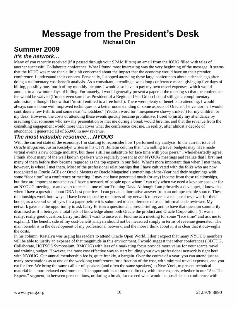
Message from the President’s Desk Michael Olin

Summer 2009 It’s the network… Many of you recently received (if it passed through your SPAM filters) an email from the IOUG filled with tales of another successful Collaborate conference. What I found most interesting was the very beginning of the message. It seems that the IOUG was more than a little bit concerned about the impact that the economy would have on their premier conference. I understand their concern. Personally, I stopped attending these large conferences about a decade ago after doing a rudimentary cost-benefit analysis. As a consultant, attending a weeklong conference meant giving up five days of billing, possibly one-fourth of my monthly income. I would also have to pay my own travel expenses, which would amount to a few more days of billing. Fortunately, I would generally present a paper at the meeting so that the conference fee would be waived (I’m not even sure if as President of a Regional User Group I could still get a complimentary admission, although I know that I’m still entitled to a free lunch). There were plenty of benefits to attending. I would always come home with improved techniques or a better understanding of some aspects of Oracle. The vendor hall would contribute a few t-shirts and some neat “tchotchkes” (Yiddish word for “inexpensive showy trinket”) for my children or my desk. However, the costs of attending these events quickly became prohibitive. I used to justify my attendance by assuming that someone who saw my presentation or met me during a break would hire me, and that the revenue from the consulting engagement would more than cover what the conference cost me. In reality, after almost a decade of attendance, I generated all of $5,000 in new revenue. The most valuable resource….NYOUG With the current state of the economy, I’m starting to reconsider how I performed my analysis. In the current issue of Oracle Magazine, Justin Kestelyn writes in his OTN Bulletin column that “Dwindling travel budgets may have made virtual events a new cottage industry, but there’s still no substitute for face time with your peers.” I wholeheartedly agree. I think about many of the well known speakers who regularly present at our NYOUG meetings and realize that I first met many of them before they became regarded as the top experts in our field. What’s more important than when I met them, however, is where I met them. Most of the professional relationships that I have cultivated with the folks who are now recognized as Oracle ACEs or Oracle Masters or Oracle Magazine’s something-of-the-Year had their beginnings with some “face time” at a conference or meeting. I may not have generated much (or any) income from these relationships, but they are important nonetheless. I have a network of people upon whom I can rely when we need a keynote speaker for an NYOUG meeting, or an expert to teach at one of our Training Days. Although I am primarily a developer, I know that when I have a question about DBA best practices, I can get an authoritative answer from an unimpeachable source. These relationships work both ways. I have been tapped by members of my network to serve as a technical reviewer for their books, as a second set of eyes for a paper before it is submitted to a conference or as an informal code reviewer. My network gave me the opportunity to ask Larry Ellison a question at a press briefing, and to have that question summarily dismissed as if it betrayed a total lack of knowledge about both Oracle the product and Oracle Corporation. (It was a really, really good question, Larry just didn’t want to answer it. Find me at a meeting for some “face time” and ask me to explain.). The benefit side of my cost-benefit analysis should not be measured simply in terms of revenue generated. The main benefit is in the development of my professional network, and the more I think about it, it is clear that it outweighs the costs. In his column, Kestelyn was urging his readers to attend Oracle Open World. I don’t expect that many NYOUG members will be able to justify an expense of that magnitude in this environment. I would suggest that other conferences (ODTUG, Collaborate, HOTSOS Symposium, RMOUG) with less of a marketing focus provide more value for your scarce travel and training budget. However, the most cost effective way to start building your own professional network is right here, with NYOUG. Our annual membership fee is, quite frankly, a bargain. Over the course of a year, you can attend just as many presentations as at one of the weeklong conferences for a fraction of the cost, with minimal travel expenses, and you eat for free. We bring the same caliber of speakers (and often the same speakers) to New York, to present technical material in a more relaxed environment. The opportunities to interact directly with these experts, whether in our “Ask The Experts” segment, in between presentations, or during a break, far exceed what would be possible at a conference with

www.nyoug.org 212.978.8890 10

10,000 attendees. Our Training Days program has been an incredible success. We are able to provide training on the same topics that are available from commercial vendors (or Oracle University), with classes run by the same experts, at discounts that approach 75%. In many cases, our Training Days are the only place that some of the top experts in the field give classes. Still building…. We still need to do more to increase both the scope and value of the network you can build through NYOUG. Our group has a paid membership of over 700 and that is less than 20% of the size of our mailing list. The number of members who actually show up in person to one of our events amounts to less than a third of our paid membership. The more involved we become as a community of users, the more valuable that network becomes to all of us. How? 1. We can continue to keep our costs and fees low by generating more revenue from our membership and vendor

sponsors. If we have more members attending our meetings, we can more easily attract vendors as sponsors. More active participants on our mailing list will make advertising in our Technical Journal more attractive. We remain steadfast in our commitment to never sell your contact information or allow marketing presentations at our meetings. Our sponsors respect this policy, but they also recognize that being able to reach our membership on our terms is still profitable. Maintaining our current fee structure will allow us to continue to increase our membership numbers.

2. Increasing involvement by our members expands all of our opportunities for networking. If you don’t attend our general meetings, come to one. If you can’t get away from the office during the day, attend one of our evening SIG meetings. See if your manager can work the modest expense (just a few hundred dollars which also includes a year membership) of one of our Training Days into the department’s budget. Take advantage of the opportunities NYOUG provides for “face time” with your peers. Start building your own professional network.

3. If you absolutely can’t make it in person (or even if you do), join our network online. NYOUG set up a group on the professional networking site LinkedIn in late 2008. We have less than 100 members in our group out of a list of close to 4,000. There is another Oracle focused group on LinkedIn called “Oracle Pro”. This group has over 8,000 members located worldwide. A quick survey of activity on both groups makes the value of a larger network clear. Since its inception, we have had 2 job openings and perhaps one technical question posted on the NYOUG LinkedIn group. The Oracle Pro group has a few job opportunities posted to it each week. Technical questions are posted daily. NYOUG is one of the largest, most active, regional users groups affiliated with the IOUG. If we could get a majority of our members engaged online, the NYOUG group on LinkedIn would become a valuable virtual network for all of us. Take a look; it’s free.

Don’t underestimate the value of your NYOUG network. Become more involved. Cultivate your professional relationships with your peers in the broader Oracle universe. Come to our meetings, take advantage of our training opportunities and join us online. Writing this column helped me realize just how important my network is. I hope you come to the same conclusion.

Upcoming Meeting Dates ODTUG Kaleidoscope 2009 DATE: June 21-25, 2009 LOCATION: Monterey, CA REGISTRATION: http://www.odtugkaleidoscope.com ------------------------------------------------------------------------- Oracle OpenWorld 2009 DATE: October 11-15, 2009 LOCATION: San Francisco, CA REGISTRATION: http://www.oracle.com/us/openworld/index.htm

www.nyoug.org 212.978.8890 11

http://www.odtugkaleidoscope.com/

http://www.oracle.com/us/openworld/index.htm

Virtual Partitioning in Oracle VLDWs

Brian Dougherty, CMA Consulting Services

Introduction Oracle 10gR2 has continued to expand upon its extensive table partitioning capabilities, providing an arsenal of weapons targeting Very Large Data Warehouse (VLDW) environments. Major partitioning schemes such as Range, Hash, and List, and Composite partitioning schemes such as Composite Range/Hash and Range/List have given architects of very large databases tools to effectively reduce search space size against large fact tables. In addition, indexing techniques such as bitmap indexes, index partitioning (bitmap and btree), bitmap-join indexes, and function-based indexes provide the ability to address high cardinality plans written against large fact tables with precise lookups. All of the above-mentioned product features of Oracle 10gR2 provide an excellent means for addressing the following large fact table “query problem spaces”: • Scanning of intensive range based queries which specify, in the query predicate, a column matching a single column

partitioning key • Scanning of intensive range based queries which specify, in the query predicate, columns which match both columns

from a multi-range (range/range) partitioning key , or at least the high-order column from a multi-range partitioning key

• Scanning of intensive queries which specify an equality or in-list predicate against a Hash Partitioned or List Partitioned table

• Scanning of intensive queries which specify a combination of range and equality or in-list predicates against various forms of composite partitioning, including Range/Hash and Range/List

With proper knowledge of the product, each of these query scenarios can be handled quite well with out-of-the-box Oracle 10gR2 partitioning. This, along with Oracle’s 10gR2 advanced partitioned bitmap indexes and bitmap join indexes places a very powerful industry leading product at the architect’s disposal. A Powerful but Incomplete Arsenal for the VLDW Architect - The Problem Defined Even given these robust, industry-leading Oracle Partitioning capabilities, there still exists a problem or point of vulnerability for the very large data warehouse query space, both for RAC and non-RAC implementations. Oracle as of Oracle 10gR2, does not provide an efficient method for tables to be simultaneously partitioned by two or more statistically independent columns. In other words, two distinct, unrelated (unrelated with respect to how the data values within the column domains occur) partitioning key columns cannot be simultaneously defined. This limitation is not addressed by composite or multi-column range partitioning because these partitioning schemes imply a relationship between at least two columns—a high order column and second order column qualified within the high order column. Conceptually, this capability would provide two separate, independent inversion entries into the table query space map, similar in nature to a cube. Both inversion entries would be equally powerful with respect to their range based filtering acumen, regardless of the column specified in the query. The following situations present challenges for current Oracle Partitioning technology when used as a sole means for implementing comprehensive partitioning pruning and therefore heightened query speedup. First, for very large fact tables (multi-terabyte in size) there are often several critical access columns used to filter table data. Moreover, the user population, often including thousands of users, is somewhat evenly split in their application of filters against these two (or more) candidate key columns. The New York State Medicaid domain area will be used to illustrate this problem. These fact tables can contain upwards of 4 billion rows of Medicaid claims and are comprised of associated search space sizes of two (2) Terabytes, for a single table. Two columns of keen interest with respect to filtering claim data are claim service date and claim payment date.

www.nyoug.org 212.978.8890 12

Roughly 60% of the queries over a month may filter by service date and 40% filter by payment date. As a result, a single column partition key design, by definition, cannot adequately provide significant search space reduction (i.e., filtering capability) against both types of queries, service date and payment date. Either the partition key is defined against service date, thus sacrificing adequate payment date filtering or it is defined against payment date, sacrificing adequate service date filtering. Second, the two candidate columns for partitioning (payment date and service date) have only a loose statistical correlation. The actual data points for each date column do not move together in a highly precise and predictable manner. In the case of service date and payment date, there is a weak lag correlation; however because of adjustments and payment variations, payment date and service dates can be quite “far away” with respect to time for a given set of claims. The actual values for these dates may be many months or even years apart for some claims. Neither multi-column range nor composite partitioning can provide reliable contiguous segment partition pruning or even reliable, consistent in-list non-contiguous pruning for both columns simultaneously. Either the data is stored on the Oracle block in a contiguous manner based on one date (e.g., service date) or the other (e.g. payment date). It cannot be stored in a contiguous manner for both. Third, four to five billion row tables render even very high cardinality columns to a weak filter status. In the Medicaid case described above, there are 5 billion claims spread over 5 million recipients. While this provides a .1% filter, 5 million rows still qualify as candidates. Although Oracle will “resolve” the bitmap very quickly using compressed bitmap indexes and parallel query plans, it will still take many minutes or even hours to perform 5 million logical (and possibly physical ) I/Os against the 5 billion row fact table. This observation illustrates the vulnerability of partitioning on one of the two major filtering columns ( e.g., service date) and addressing all other entries, including payment date by indexing. Note: An underlying premise here is the fact that most Oracle index I/O (not withstanding Fast Full Index Scans) is implemented as single block SGA buffered I/O, whereas non-index I/O in this environment is implemented as multi-block direct path I/O in chunks of up to 1MB (SSTIOMAX). This fact, combined with a parallel plan, and capable storage platform quickly shift the advantage to partition pruned parallel direct path I/O instead of single block index I/O, even when bitmap indexes are employed. In summary, Very Large Data Warehouses containing billion row fact tables with diverse query patterns and statistically independent columns, both of which have a somewhat equal chance of becoming a primary range filter, provide a difficult design challenge for the VLDW architect. The Architectural Solution - Virtual Partitioning Virtual Partitioning is defined here as the ability for the Oracle Optimizer to recognize and execute several or many independent segment pruning paths into the same table. This can be accomplished by building and storing the same large fact table several times and then associating a different partitioning scheme with each representation of the table. This allows an intelligent router (e.g., the oracle optimizer) to transparently route the query against the table representation presenting the most efficient pruning scheme. This implementation comes at the expense of n times the storage requirement. The ultimate solution would store the very large table segment once but provide several different, independent partitioning schemes. These schemes would allow for Direct Path multi-block I/O against a subset of table partitions. The most efficient but most impractical solution would provide the ability to “reorganize” data in contiguous blocks dynamically. This dynamic “reorganization” would be based on the partition pruning scheme best suited to position the query for direct path multi-block I/O against a contiguous range of blocks; in other words this would represent a kind of “just-in-time” partitioning. A less efficient but more practical solution would provide the ability to store the data in a base way (the storage layer), but also provide for multiple I/O partition pruning schemes via sets of non-contiguous block lists (similar to an index). This would be coupled with an optimized I/O scanning layer providing for a skip-sequential, multi-block direct path I/O capability. This solution would consist of several virtual, but not actual, physical partitioning schemes against the same underlying table.

www.nyoug.org 212.978.8890 13

Speculating into the Oracle product future, perhaps a more practical method for implementation would provide an enhanced table abstraction, in the form of a kind of super-table collection, encapsulating n significantly compressed (e.g. 70-80% compression) tables, each with its own distinct table partitioning, but with the exact same column definition. This would be designed to work in concert with an enhanced oracle optimizer whose job would be to route range queries to the proper “collection sub-table”, taking into consideration the underlying partitioning schemes and the query. Of course, any type of table DML would need to “broadcast” any table/row changes to all “sub-tables” and synchronize the update, in a read-intensive environment. This may be an acceptable trade-off in a VLDW read intensive environment. The Interim Solution – Simulated Virtual Partitioning using Oracle 10gR2 Materialized Views and Query Re-Write Although Oracle Version 11g with Ref partitioning , interval partitioning, and virtual columns is laying the foundation for Virtual Partitioning, the implementation still may be several releases away. In the meantime, we can simulate Virtual Partitioning and the ability to “dynamically re-organize” the table to fit the query pruning problem by employing Oracle 10gR2 Materialized Views. This will provide a practical means to transparently route queries to a more “partition pruned optimized” version of the base table. While typically used as a means to provide speed-up for fact table aggregates and/or aggregate joins, Oracle 10gR2 Materialized Views and query re-write provide excellent underlying technology to implement routing of queries to more structurally optimized fact table replicates. Using Materialized Views to implement this capability provides an order of magnitude speed up (many minutes or even hours) for range-based queries. However, there are two, often acceptable, drawbacks: • An increase in storage to n times the base table (although quite often it is not necessary to store the complete fact table

many times); and • Less than 100% query re-write reliability (although practically speaking more than reliable enough to provide

measurable value). Assuming that these trade-offs are acceptable, how can Virtual Partitioning be implemented? Implementing Virtual Partitioning using Oracle 10g Materialized Views The following describes an example along with the steps required to implement Virtual Partitioning. Consider one large fact table with several dimensions, modeled in a star schema, in this case, a CLAIM_FACT table with a PROVIDER_DIMENSION, FORMULARY DIMENSION, and DATE DIMENSION. The following attributes define the large fact table: • 4 billion rows • 100 columns • 500 bytes internal row length • Compressed table • 15 years of claim data • Two prevalent date range filters (e.g., service date and payment date) and thousands of potential range based queries

per week For the above scenario, the following steps are required to implement Virtual Partitioning: 1. Define the primary fact table (CLAIM_FACT) using an actual partitioning scheme against one of the primary range

based filters (e.g., service date). Implement Oracle 10gR2 Range based partitioning to implement the actual base table partitioning. Map the CLAIM_FACT table to a first set of tablespaces to distribute I/O load.

2. Create a second instantiation (replicate) of CLAIM_FACT called CLAIM_FACT_PAYMENT . This table does not necessarily contain all years, for example perhaps only the most current seven years of the fifteen, but does contain all columns. Inclusion of all columns increases the probability that Oracle will choose query re-write against the second fact table, for all appropriate queries. Use Oracle 10gR2 Range based Partitioning to partition the second fact table by what will be defined as the first virtual (virtual relative to base table) partitioning scheme. For example, implement Oracle 10gR2 Range based Partitioning on payment date where payment date becomes a virtual partitioning scheme against the base table

www.nyoug.org 212.978.8890 14

CLAIM_FACT by way of query re-write and Oracle Materialized Views. Finally, map the second instantiation of the base table to a second set of I/O optimized tablespaces leveraging different disk volumes. (Note: A third Virtual partitioning scheme could be defined if a third prevalent partitioning pruning column existed and so on)

3. Register the second instantiation of the primary fact table (i.e., CLAIM_FACT_PAYMENT) as an Oracle 10gR2 Materialized View with query re-write enabled (the other attributes of the materialized view definition are less critical for this exercise). This will allow the second table, which is partitioned on the alternative partitioning key (payment date) and which includes all columns from the base table, to be a candidate for Oracle 10gR2 query re-write. In this situation, queries submitted against the original CLAIM_FACT table are candidates to be transparently re-routed to the second fact table, CLAIM_FACT_PAYMENT. This will most appropriately occur when the query contains a range based filter on payment date In a related note, indexes on the second fact table (i.e., the Materialized View) are not required because they provide little benefit for the scenarios defined. Once an index is deemed beneficial, it should be defined as one or several bitmap indexes on the original instantiation of the fact. Indexes on the second instantiation of the fact table will increase the overall cost of the solution because of additional index re-build time and disk space.

4. Determine optimal data population (load) schemes for base and replicate tables (Materialized Views). An effective ETL load scheme might load fact rows into both fact tables directly (i.e., base fact table and the materialized view) and then simply drop and re-register the materialized view. Others exist however, including loading the primary fact table directly and building the materialized view from the primary fact table. In either case the final step is the re-registration.

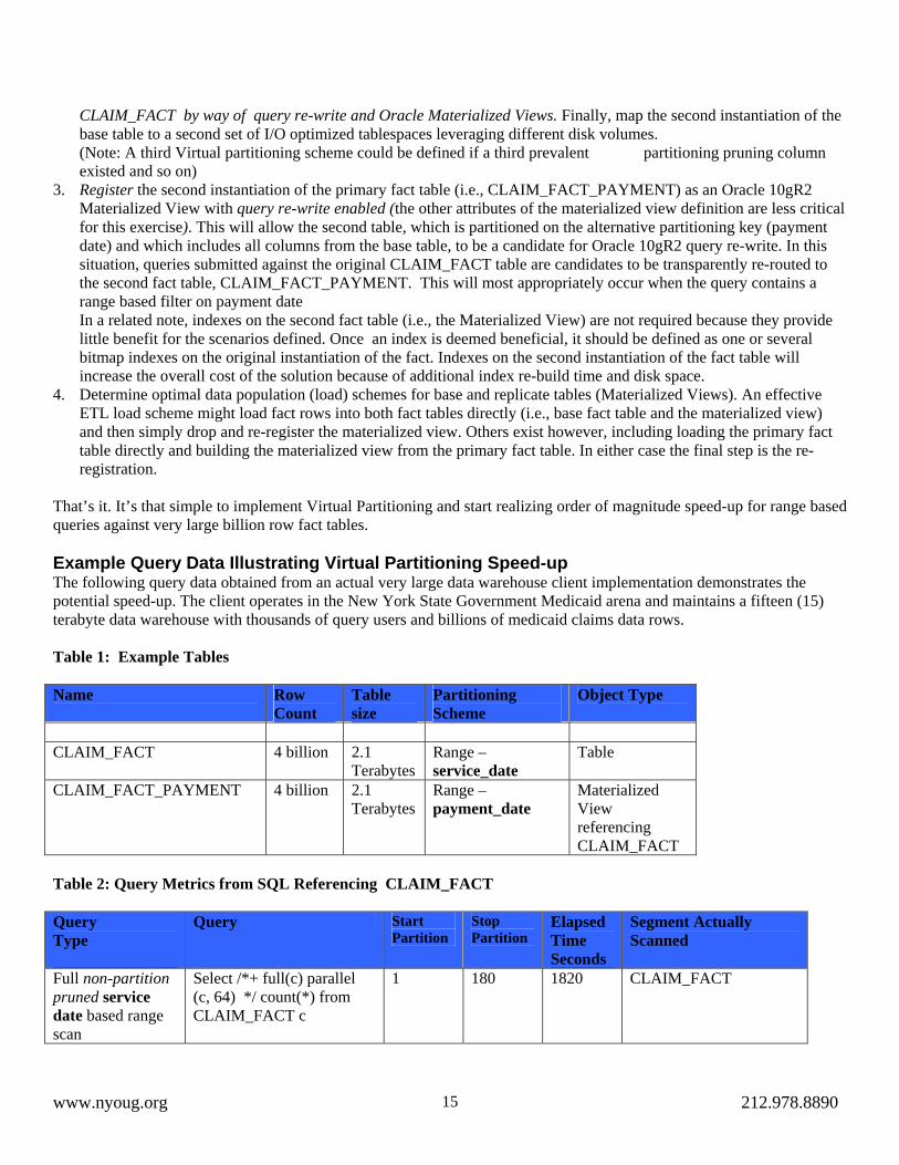
That’s it. It’s that simple to implement Virtual Partitioning and start realizing order of magnitude speed-up for range based queries against very large billion row fact tables. Example Query Data Illustrating Virtual Partitioning Speed-up The following query data obtained from an actual very large data warehouse client implementation demonstrates the potential speed-up. The client operates in the New York State Government Medicaid arena and maintains a fifteen (15) terabyte data warehouse with thousands of query users and billions of medicaid claims data rows. Table 1: Example Tables Name Row

Count Table size

Partitioning Scheme

Object Type

CLAIM_FACT 4 billion 2.1

Terabytes Range – service_date

Table

CLAIM_FACT_PAYMENT 4 billion 2.1 Terabytes

Range – payment_date

Materialized View referencing CLAIM_FACT

Table 2: Query Metrics from SQL Referencing CLAIM_FACT Query Type

Query Start Partition

Stop Partition

Elapsed Time Seconds

Segment Actually Scanned

Full non-partition pruned service date based range scan

Select /*+ full(c) parallel (c, 64) */ count(*) from CLAIM_FACT c

1 180 1820 CLAIM_FACT

www.nyoug.org 212.978.8890 15

Full partition pruned service date based range scan

Select /*+ full(c) parallel (c, 64) */ count(*) from CLAIM_FACT c where service_date between ’01-JAN-2005’ and ’31-DEC-2006’


Full non-partition pruned payment date based range scan Forcing no rewite with the No rewrite hint

Select /*+ full(c) parallel (c, 64) no_rewrite */ count(*) from CLAIM_FACT c where payment_date between ’01-JAN-2005’ and ’31-DEC-2006’


Full partition pruned payment date based range scan using Virtual Partitioning Same query as above but allow query re-write

Select /*+ full(c) parallel (c, 64) */ count(*) from CLAIM_FACT c where payment_date between ’01-JAN-2005’ and ’31-DEC-2006’

164 176 280** CLAIM_FACT_PAYMENT Oracle 10gR2 Materialized View

** 5 minutes vs. 30+ minutes for the non- Virtual Partitioning case Conclusion Pending the release of partitioning schemes which provide speed-up of scan intensive range queries containing two or more statistically independent columns, Virtual Partitioning using Oracle 10gR2 Materialized Views and query re-write provide a valuable interim solution. The combination of Oracle 10gR2 Materialized Views and Oracle Partitioning provides a means to simulate multiple independent partitioning keys on the same billion row fact table, thus providing a virtual partitioning scheme against the base fact table. This approach is especially valuable within the context of large fact tables because, on this scale, bitmap indexes provide diminishing utility due to weaker absolute filtering capacity. This fact coupled with the nature of single block based indexed I/O ( manifested as db file sequential read wait event) make a compelling case for enhanced pruning capabilities. Virtual Partitioning utilizing Oracle 10gR2 Materialized views and query write provide a bridge to the future. Brian Dougherty is Chief Data Warehouse Architect for CMA Consulting Services. He was lead architect for the 1999 Data Warehouse Institute’s Best Practice award winner in the Very Large Data Warehouse Category. His solutions have also been nominated for various other awards including the Computerworld Smithsonian Institute and Harvard’s Kennedy School of Government Excellence in Technology. He is also author of the Component Based Framework, an object oriented framework for delivering large scale data warehouses.

www.nyoug.org 212.978.8890 16

Performance Tuning Web Applications

Dr. Paul Dorsey and Michael Rosenblum, Dulcian, Inc. The main performance tuning techniques applied to client/server applications consisted of rewriting poorly written SQL code and tuning the database itself. These two techniques covered all but the most pathologically badly written applications. However, in contrast, web applications are frequently unaffected by these .performance improvement approaches. The causes of a slowly running web applications are often different from those of client/server applications. Typical Web Application Process Flow Poorly written SQL and a badly designed database will make any application run slower, but to improve performance of a poorly performing web application requires examination of the entire system, not just the database. A typical 3-tier web application structure is shown in Figure 1. (Note the numbering of the areas in the diagram since these will be used throughout this paper).

3. Application Server2. Send data from

Client to App Server 5. Database

6. Return Data from DB to App Server

1. Client4. Send data from

App Server to DB

7. Data in Application Server

8. Return data from App Server to client

9. Data in client

3. Application Server2. Send data from

Client to App Server 5. Database

6. Return Data from DB to App Server

1. Client4. Send data from

App Server to DB

7. Data in Application Server

8. Return data from App Server to client

9. Data in client

Figure 1: Web Application Process Flow

As shown in Figure 1, there are numerous possible places for web applications to experience bottlenecks or performance killers as described in the following nine step process: Step 1: Code and operations executed on the client machine - When a user clicks a “Submit” button, data is

collected and bundled into a request that is sent to the application server. Step 2: Transmission of client request to the application server Step 3: Code in the application server executed as a formulation of the client request to retrieve information from

the database. Step 4: Transmission of request from application server to the database Step 5: Database reception, processing and preparation of return information to the application server. Step 6: Transmission over internal network of information from database to the application server Step 7: Application server processing of database response and preparation of response transmission to the client

machine. Step 8: Transmission of data from the application server to the client machine Step 9: Client machine processing of returned request and rendering of application page in browser.

www.nyoug.org 212.978.8890 17

Possible Web Application Performance Problem Areas Traditional tuning techniques only help with Step 5 and ignore all of the other eight places where performance can degrade. This section describe how problems can occur at each step of the process. Step 1. Client Machine Performance Problems The formulation of a request in the client is usually the least likely source of system performance problems. However, it should not be dismissed entirely. Using many modern AJAX architectures, it is possible to place so much code in the client that a significant amount of time is required before the request is transmitted to the application server. This is particularly true for underpowered client machines with inadequate memory and slow processors. Step 2. Client to Application Server Transmission Problems Like the client machine itself, the transmission time between the client machine and the application server is a less common cause of slowly performing web applications. However, if attempting to transmit a large amount of information, the time required to do so over the Internet may be affected. For example, uploading large files or transmitting a large block of data may slow down performance. Step 3. Application Server Performance Problems The application server itself rarely causes significant performance degradation. For computationally intensive applications such as large matrix inversions for linear programming problems, some performance slowdowns can occur, but this is less likely to be a significant factor in poorly performing applications. Step 4. Application Server to Database Transmission Problems Transmission of data from the application server to the database with 1 GB or better transmission speeds might lead you to ignore this step in the process. It is not the time needed to move data from the application server to the database that causes performance degradation but it is the high number of transmission requests. The trend in current web development is to make applications database-independent. This sometimes results in a single request from a client requiring many requests from the application server to the database in order to fulfill. What needs to be examined and measured is the number of roundtrips made from the application server to the database. Inexpert developers may create routines that execute so many roundtrips that there is little tuning that a DBA can do to yield reasonable performance results. It is not unusual for a single request from the client to generate hundreds (if not thousands) of round trips from the application server to the database before the transmission is complete. A particularly bad example of this encountered by the authors required 50,000-100,000 round trips. Why would this large number be needed? Java developers who think of the database as nothing more than a place to store persistent copies of their classes use Getters and Setters to retrieve and/or update individual attributes of objects. This type of development can generate a round trip for every attribute of every object in the database, which means that inserting a row into a table with 100 columns results in a single Insert followed by 99 Update statements. Retrieving this record from the database then requires 100 independent queries. In the application server, identifying performance problems involves counting the number of transmissions made. The accumulation of time spent making round trips is one of the most common places where web application performance can suffer. Step 5. Database Performance Problems In the database itself, it is important to look for the same things that cause client/server applications to run slowly. However, additional web application features can cause other performance problems in the database. Most web applications are stateless, meaning that each client request is independent. Developers do not have the ability to use package variables that persist over time. Consequently, when a user logs into an application, he/she will be making multiple requests within the context of the sign-on operation. The information pertaining to that session must be retrieved at the beginning of every request and persistently stored at the end of every request. Depending upon how this persistence

www.nyoug.org 212.978.8890 18

is handled in the database, a single table may generate massive I/O demands resulting in redo logs full of information which may cause contention on tables where session information is stored. Step 6. Database to Application Server Transmission Problems Transferring information from the database back to the application server (similar to Step 4) is usually not problematic from a performance standpoint. However, performance can suffer when a Java program requests a single record from a table. If the entire table contents are brought into the middle tier and then filtered to find the appropriate record, performance will be slow. The application can perform well as long as data volumes are small. As data accumulates, the amount of information transferred to the application server becomes too large, thus affecting performance. Step 7. Application Server Processing Performance Problems Processing the data from the database can be resource-intensive. Many database-independent Java programmers minimize work done in the database and execute much of the application logic in the middle tier. In general, complex data manipulation can be handled much more efficiently with database code. Java programmers should minimize information returned to the application server and, where convenient, use the database to handle computations. Step 8. Application Server to Client Machine Transmission Problems This area is one of the most important for addressing performance problems and often receives the least attention. Industry standards often assume that everyone has access to high performance client machines so that the amount of data transmitted from the application server to the client is irrelevant. As the industry moves to Web 2.0 and AJAX, very rich UI applications create more and more bloated screens of 1 megabyte or more. Some of the AJAX partial page refresh capabilities mitigate this problem somewhat (100-200K). Since most web pages only need to logically transmit an amount of information requiring 5K or less, the logical round trips on an open page should be measured in tens or hundreds of characters rather than megabytes. Transmission between the application server and the client machine can be the most significant cause of poor web application performance. If a web page takes 30 seconds to load, even if it is prepared in 5 rather than 10 seconds, users will not experience much of a benefit. The amount of information being send must be decreased. Step 9. Client Performance Problems How much work does the client need to do to render a web application page? This area is usually not a performance killer, but it can contribute to poor performance. Very processing-intensive page rendering can result in poor application performance. Locating the Cause of Slowly Performing Web Applications In order to identify performance bottlenecks, timers must be embedded into a system to help ascertain which of the nine possible places the application performance is degrading. Most users will say “I clicked this button and it takes X seconds until I get a response.” This provides no information about which area or combination of areas is causing this slow performance. Strategically placed timers will indicate how much time is spent at any one of the nine steps in the total process. Using Timers to Gather Data About Slow Performance This section describes the strategy for collecting information to help pinpoint web application bottlenecks. Steps 1 & 9 Placing timers in the client machine is a simple task. A timer can be placed at the beginning and end of the client-side code.

www.nyoug.org 212.978.8890 19

Steps 2 & 8 Transmissions to and from the application server are difficult to directly measure. If you can ensure that the clocks on the client and application server are exactly synchronized, it is possible to put time stamps on transmissions, but the precise synchronization is often very difficult. A better solution is to determine the sum of time required for these two transmissions by measuring the total time from transmission to reception at the client and subtracting the amount of time spent from when the application server received the request and sent it back. This information will not reveal whether or not the problem is occurring during Step 2 or Step 8, but it will detect whether or not the problem is Internet related. If the problem is related to slow Internet transmission, the cause is likely to be large data volume. This can be tested by measuring round trip time required to send and retrieve varying amounts of information. Steps 3-7 The time spent going from the application server to the database and back is easy to measure by calculating the difference between the timestamps at the beginning and end of a routine. Depending upon how the system is architected, breaking down the time spent between Steps 1-3 can be very challenging. The processing time to/from the database can be very difficult to measure. Most Java applications directly interface with the database in multiple ways and placed in the code. There is no isolated servlet through which all database interaction passes. In the database itself, if the application server sends many requests from different sessions, the database cannot determine which information is being requested by which logical session, making it very difficult to get accurate time measures. If the system architecture includes Java code that makes random JDBC calls, there is no way to identify where a performance bottleneck is occurring between Steps 3-7. Time stamps would be needed around each database call to provide accurate information about performance during this part of the process. A more disciplined approach for calling the database is needed. This can be handled in either the application server or the database. For the application server, a single servlet can be created through which all database access would pass to provide a single place for placing timestamps. This servlet would gather information about the time spent in the application server alone (Steps 3 & 7) as well as the sum of Steps 4, 5, and 6 (to/from and in the database). Since the time in the database (4 & 6) will be negligible, this is an adequate solution. To measure the time spent in the database, create a single function through which all database access is routed. The session ID would be passed as a parameter to the function to measure the time spent in the database as well as the number of independent calls. Solving Web Application Performance Problems Solving the performance problems in each of the nine web application process steps requires different approaches, depending upon the location of the problem. Solving Client Machine Performance Problems (Steps 1 & 9) Performance degradations in the client machine are usually due to AJAX-related page bloat burdening the client with rich UI components that could be eliminated. Determine whether all functionality is needed in the client. Can some processing be moved to the application server, database, or eliminated entirely? Resolving Performance Issues between the Client and Application Server (Step 2) If the performance slowdown occurs during the transmission of information from the client to the application server, you need to decide whether or not any unnecessary information is being sent. To improve performance, decrease the amount of information being transmitted or divide that information into two or more smaller requests. This will reduce the perceived performance degradation. Making web pages smaller or creating more smaller web pages is also a possibility.

www.nyoug.org 212.978.8890 20

Solving Performance Problems in the Application Server (Step 3 & 7) If the application server is identified as a bottleneck, examine the code carefully and/or move some logic to the database. If too many roundtrips are being made between the application server and the database, are Getters/Setters being overused? Is one record being retrieved with a single query when a set can be retrieved? If performance cannot be improved because the program logic requires bundles (or thousands of round trips), rewrite Java code in PL/SQL and move more code into the database. Solving Performance Problems in the Client (Step 9) If too much information is being moved to the client, the only solution is to reduce the amount of that information. Changing architectures, making web pages smaller, removing AJAX code, and removing or reducing the number of images may help. Analyze each page to determine why it may be so large and reduce its memory size or divide it into smaller multiple pages. Measuring Performance Simply understanding a 9-step tuning process is not enough to be able to make a system work efficiently/ There should be a formal, quantitative way to measure performance. Necessary vocabulary: • Command is an atomic part of the process (any command on any tier) • Step is a complete processing cycle in one direction (always one-way) that can either be a communication step

between one tier and another, or a set of steps within the same tier. A step consists of a number of commands • Request is an action consisting of a number of steps. A request is passed between different processing tiers. • Round-trip means a complete cycle from the moment the request leaves the tier to the point when it returns with

some response information. Under the best of circumstances, the concept of a round-trip is redundant, but in real life getting precise measurements for all nine steps is extremely complicated: • Steps 1,3,5,7,9 – both the start and finish of the step are within the same tier and the same programming environment • Steps 2,4,6,8 – start and end are in different tiers. Having entry points in different tiers means that there must be time synchronization between tiers, otherwise time measurements are completely useless. This problem can be partially solved in closed networks (like MilNet); but for the majority of Internet-based applications, it is a roadblock since there is no way to get reliable numbers. The concept of a “round-trip” enables us to get around this issue. The 9-step model could be also represented as shown in Figure 2.

www.nyoug.org 212.978.8890 21

Figure 2: Round-TripTiming of 9-step process

80 sec 100 sec

75 sec 50 sec 40 sec

40

4

6

15

10

2

3

5

15

Client App

server

DATABASE

Client App server DATABASE

At the client level: 1. From the moment that a request was initiated to the end of processing (user clicked the button/response is displayed) 2. From the moment that a request was sent to the application server to the moment a response was received (start of

servlet call/ end of servlet call) At the application server level: 3. From the moment that a request was accepted to the moment a response was sent back (start of processing in the

servlet/end of processing in the servlet) 4. From the moment that a request was sent to the database (start of JDBC call / end of JDBC call) At the database level 5. From the moment that a request was accepted to the moment a response was sent back (start of the block/end of the

block) Now there is a “nested” set of numbers that are 100% valid because they are measured on the same level. This allows us to calculate the following: • Total time spent between the client and application server both ways (step 2 + step 8) = round trip 2 minus round trip

3 • Total time spent between the application server and the database both ways (step 4 + step 6) = round trip 4 minus

round trip 5 Although there is no way to reduce this to a single step, but it is significantly better than no data at all, because two-way timing provides a fairly reliable understanding of what percentage of the total request time is lost during these network operations. These measurements provide enough information to make appropriate decisions about where to spend the most tuning resources, which is the most critical decision in the whole tuning process.

www.nyoug.org 212.978.8890 22

Conclusions There is much more to tuning a web application than simply identifying slow database queries. Changing database and operating system parameters will only go so far. The most common causes of slow performance are as follows: 1. Excessive round trips from the application server to the database - Ideally, each UI operation should require

exactly one round trip to the database. Sometimes, the framework (such as ADF) will require additional round trips to retrieve and persist session data. Any UI operation requiring more than a few round trips should be carefully investigated.

2. Large pages sent to the client - Developers often assume that all of the system users have high-speed Internet connections. Everyone has encountered slow loading web pages taking multiple seconds to load. Once in a while, these delays are not significant. However, this type of performance degradation (waiting 3 seconds for each page refresh) in an application such as a data entry intensive payroll application is unacceptable. Applications should be architected to take into account the slowest possible network to support when testing the system architecture for suitability in slower environments.

3. Performing operations in the application server that should be done in the database - For large, complex systems with sufficient data volumes, complete database independence is very difficult to achieve. The more complex and data intensive a routine, the greater the likelihood that it will perform much better in the database. For example, the authors encountered a middle tier Java routine that required 20 minutes to run. This same routine ran in 2/10 of a second when refactored in PL/SQL and moved to the database.

4. Poorly written SQL and PL/SQL routines - In some organizations, this may be the #1 cause of slowly performing web applications. This situation often occurs when Java programmers are also expected to write a lot of SQL code. In most cases, the performance degradation is not caused by a single slow running routine but a tendency to fire off more queries than are needed.

Keeping all nine of the potential areas for encountering performance problems in mind and investigating each one carefully can help to identify the cause of a slowly performing web application and point to ways in which that performance can be improved. About the Authors Dr. Paul Dorsey is the founder and president of Dulcian, Inc. an Oracle consulting firm specializing in business rules and web-based application development. He is the chief architect of Dulcian's Business Rules Information Manager (BRIM®) tool. Paul is the co-author of seven Oracle Press books on Designer, Database Design, Developer, and JDeveloper, which have been translated into nine languages as well as the Wiley Press book PL/SQL for Dummies. Paul is an Oracle ACE Director. He is President Emeritus of NYOUG and the Associate Editor of the International Oracle User Group’s SELECT Journal. In 2003, Dr. Dorsey was honored by ODTUG as volunteer of the year and as Best Speaker (Topic & Content) for the 2007 conference, in 2001 by IOUG as volunteer of the year and by Oracle as one of the six initial honorary Oracle 9i Certified Masters. Paul is also the founder and Chairperson of the ODTUG Symposium, currently in its ninth year. Dr. Dorsey's submission of a Survey Generator built to collect data for The Preeclampsia Foundation was the winner of the 2007 Oracle Fusion Middleware Developer Challenge and Oracle selected him as the 2007 PL/SQL Developer of the Year. Michael Rosenblum is a Development DBA at Dulcian, Inc. He is responsible for system tuning and application architecture. He supports Dulcian developers by writing complex PL/SQL routines and researching new features. Mr. Rosenblum is the co-author of PL/SQL for Dummies (Wiley Press, 2006). Michael is a frequent presenter at various regional and national Oracle user group conferences. In his native Ukraine, he received the scholarship of the President of Ukraine, a Masters Degree in Information Systems, and a Diploma with Honors from the Kiev National University of Economics.

www.nyoug.org 212.978.8890 23

www.pillardata.com

Pillar Axiom® can more than double your efficiency in running Oracle applications, because it sees storage from an applications point of view.

Pillar’s integrated support for Oracle Enterprise Manager provides an ideal platform for monitoring

your application SLAs. Since Pillar is Application-Aware, business policies are easily enforced and automated for Oracle E-Business Suite, PeopleSoft, Siebel, JD Edwards, and Retek.

Pillar’s support for Oracle Validated Configurations assures a faster, easier, lower-cost platform for all Oracle 11g Database and BI/DW customers, too. And Pillar and Oracle provide joint accelerator solutions for customers looking to expedite database and applications upgrades.

Find out why Oracle chose Pillar to eliminate cost and drive the highest level of efficiencies. And how we can do the same for you, with Application-Aware storage for Oracle applications. They’re made for each other, so you can get the best out of both of them.

Call 1.877.252.3706 or visit www.pillardata.com

The First and Only TrueApplication-Aware StorageTM

© 2008 Pillar Data Systems Inc. All rights reserved. Pillar Data Systems, Pillar Axiom, AxiomONE and the Pillar logo are all trademarks or registered trademarks of Pillar Data Systems.

OracleE-Business Suite

JD Edwards

PeopleSoft

Siebel

Application-Aware Storage forOracle Applications.

Application-Aware Storage forOracle Applications.

Retek

Pillar Axiom.Pillar Axiom.

Listening In: Passive Capture and Analysis of Oracle Network Traffic

Jonah H. Harris, myYearbook.com

Overview In this presentation we will discuss the Oracle wire-level protocol and demonstrate the methods for passively capturing, analyzing, and reporting the details of Oracle network traffic in real-time for use in end-to-end Oracle tuning and troubleshooting scenarios. In cases where very short response time requirements must be met, or where sporadic spikes in response time occur, the most reliable way to tune and troubleshoot them is by capturing Oracle's Ethernet traffic, analyzing it, and reporting on various aspects of it. Throughout this session we will demonstrate the passive capture of SQL statements, their frequency, time spent in execution, number of roundtrips, and all relevant response times. Using the data from these reports can not only assist DBAs in diagnosing network-related issues and in tuning Oracle's network settings, but also ensure that application developers are writing performant, network-friendly database access code. Introduction This paper introduces the concepts behind Oracle’s Network Architecture as well as protocol descriptions, an example wire-level application, and an introduction to the SCAPE4O network monitoring utility. As I’ve never been an Oracle insider, the material in this paper has been based on years of researching Oracle internals as well as analyzing network traffic and trace files. Likewise, in addition to similar research from Ian Redfern, the majority of this paper is based primarily on my own personal research and discussions with Tanel Põder; without their insight, this would’ve taken me significantly longer to rationalize. The Oracle Network Architecture Like several other databases, the Oracle network architecture is based on the Open Systems Interconnection (OSI) Basic Reference Model. The OSI model is a layered, abstract communications and computer network protocol architecture which consists of communications between separate systems being performed in a stack-like fashion; information passing from node-to-node through several distinct layers of code. The OSI Model The OSI layers consist of the following: 1. Physical Layer 2. Data Link Layer 3. Network Layer 4. Transport Layer 5. Session Layer 6. Presentation Layer 7. Application Layer The OSI Physical Layer (Layer 1) The physical layer defines all the electrical and physical specifications for devices. In particular, it defines the relationship between a device and a physical medium. This includes the layout of pins, voltages, cable specifications, Hubs, repeaters, network adapters, Host Bus Adapters (HBAs used in Storage Area Networks) and more.

www.nyoug.org 212.978.8890 25

To understand the function of the physical layer in contrast to the functions of the data link layer, think of the physical layer as concerned primarily with the interaction of a single device with a medium, where the data link layer is concerned more with the interactions of multiple devices (i.e., at least two) with a shared medium. The physical layer will tell one device how to transmit to the medium, and another device how to receive from it (in most cases it does not tell the device how to connect to the medium). Obsolescent physical layer standards such as RS-232 do use physical wires to control access to the medium. The OSI Data Link Layer (Layer 2) The data link layer provides the functional and procedural means to transfer data between network entities and to detect and possibly correct errors that may occur in the physical layer. Originally, this layer was intended for point-to-point and point-to-multipoint media, characteristic of wide area media in the telephone system. Local area network architecture, which included broadcast-capable multiaccess media, was developed independently of the ISO work, in IEEE Project 802. IEEE work assumed sublayering and management functions not required for WAN use. In modern practice, only error detection, not flow control using sliding window, is present in modern data link protocols such as Point-to-Point Protocol (PPP), and, on local area networks, the IEEE 802.2 LLC layer is not used for most protocols on Ethernet, and, on other local area networks, its flow control and acknowledgment mechanisms are rarely used. Sliding window flow control and acknowledgment is used at the transport layers by protocols such as TCP, but is still used in niches where X.25 offers performance advantages. The OSI Network Layer (Layer 3) The network layer provides the functional and procedural means of transferring variable length data sequences from a source to a destination via one or more networks while maintaining the quality of service requested by the Transport layer. The Network layer performs network routing functions, and might also perform fragmentation and reassembly, and report delivery errors. Routers operate at this layer—sending data throughout the extended network and making the Internet possible. This is a logical addressing scheme – values are chosen by the network engineer. The addressing scheme is hierarchical. The OSI Transport Layer (Layer 4) The transport layer provides transparent transfer of data between end users, providing reliable data transfer services to the upper layers. The transport layer controls the reliability of a given link through flow control, segmentation/desegmentation, and error control. Some protocols are state and connection oriented. This means that the transport layer can keep track of the segments and retransmit those that fail. The OSI Session Layer (Layer 5) The session layer controls the dialogues/connections (sessions) between computers. It establishes, manages and terminates the connections between the local and remote application. It provides for full-duplex, half-duplex, or simplex operation, and establishes checkpointing, adjournment, termination, and restart procedures. The OSI model made this layer responsible for "graceful close" of sessions, which is a property of TCP, and also for session checkpointing and recovery, which is not usually used in the Internet protocols suite. Session layers are commonly used in application environments that make use of remote procedure calls (RPCs). The OSI Presentation Layer (Layer 6) The presentation layer establishes a context between application layer entities, in which the higher-layer entities can use different syntax and semantics, as long as the Presentation Service understands both and the mapping between them. The presentation service data units are then encapsulated into Session Protocol Data Units, and moved down the stack. The OSI Application Layer (Layer 7) The application layer interfaces directly to and performs application services for the application processes; it also issues requests to the presentation layer. Note carefully that this layer provides services to user-defined application processes, and not to the end user. For example, it defines a file transfer protocol, but the end user must go through an application

www.nyoug.org 212.978.8890 26

process to invoke file transfer. The OSI model does not include human interfaces. The common application services sublayer provides functional elements including the Remote Operations Service Element (comparable to Internet Remote Procedure Call), Association Control, and Transaction Processing (according to the ACID requirements). Mapping OSI Layers to Oracle Oracle Net Services starts at the OSI Session Layer.

Oracle to OSI Mapping

Oracle Protocol Support (Layer 5) While Oracle Protocol Support sounds like it would map to Layer 4, it does not actually provide the network transport stack; making it Layer 5. Oracle Protocol Support is designed to map Transparent Network Substrate to industry-standard transport protocols using an existing protocol stack. More about this layer can be found below under Network Transport (NT). Oracle Net Foundation Layer (Layer 5) The Oracle Net foundation layer is responsible for establishing and maintaining the connection between the client application and database server, as well as exchanging messages between them. The Oracle Net foundation layer is able to perform these tasks because of a technology called Transparent Network Substrate (TNS). TNS provides a single, common interface functioning over all industry-standard protocols. In other words, TNS enables peer-to-peer application connectivity. In a peer-to-peer architecture, two or more computers (called nodes when they are employed in a networking environment) can communicate with each other directly, without the need for any intermediary devices. Two Task Common Layer (Layer 6) Character set differences can occur if the client and database server are running on different operating systems. The presentation layer resolves any differences. It is optimized for each connection to perform conversion only when required. The presentation layer used by client/server applications is Two-Task Common (TTC). TTC provides character set and data type conversion between different character sets or formats on the client and database server. At the time of initial connection, TTC is responsible for evaluating differences in internal data and character set representations and determining whether conversions are required for the two computers to communicate. Application and RDBMS Layer (Layer 7) Information passed from a client application across a network protocol is received by a similar communications stack on the database server side. The process flow on the database server side is the reverse of the process flow on the client side, with information ascending through the communication layers. Instead of OCI, the database server uses Oracle Program Interface (OPI). For each statement sent from OCI, OPI provides a response. For example, an OCI request to fetch 25 rows would elicit an OPI response to return the 25 rows once they have been fetched.

www.nyoug.org 212.978.8890 27

Mapping Example

Oracle Net Components The Oracle Net implementation stack is comprised of the following components:

Oracle Network Layer Components

Network Interface (NI) This layer provides a generic interface for Oracle clients, servers, or external processes to access Oracle Net functions. The NI layer handles the "break" and "reset" requests for a connection. Network Routing (NR) This layer routes the network session to the destination. Network Naming (NN) This layer resolves connect identifiers to connect descriptors. Network Session (NS) The NS layer, which concists of the NR and NA layers, receives requests from NI, and settles all generic computer-level connectivity issues, such as: the location of the server or destination (open, close functions); whether one or more

www.nyoug.org 212.978.8890 28

protocols will be involved in the connection (open, close functions); and how to handle interrupts between client and server based on the capabilities of each (send, receive functions). Network Authentication (NA) This layer negotiates authentication and encryption requirements. Network Transport (NT) This layer maps the Oracle Net Foundation Layer functionality to industry-standard protocols. The Oracle Network Protocol The Oracle network protocol is comprised of the following components:

Transparent Network Substrate (TNS) A foundation technology, built into the Oracle Net foundation layer that works with any standard network transport protocol. Two Task Interface (TTI) Encapsulated by TNS are Oracle's Two Task Interface sub-packets. TTI is the network-level interface to Oracle Database functionality. Two Task Common (TTC) A presentation layer type that is used in a typical Oracle Net connection to provide character set and data type conversion between different character sets or formats on the client and server. Oracle Programmatic Interface (OPI) The Oracle Program Interface (OPI) is a server-side networking layer responsible for responding to each of the possible messages sent by the client interface. Interaction with OPI is handled through TTI functions. TNS Packet Overview TNS consists of several packets which are described in the following sections. TNS Packet Types TNS packets have distinct types. • Connection Packet—The initial request packet used to connect to a database. • Accept Packet—A response packet from the server accepting the connection. • Acknowledge Packet—An acknowledgement packet. • Refuse Packet—A response packet from the server refusing connection. • Redirect Packet—A response packet from the server redirecting the client to connect to another host/port. • Data Packet—The most commonly used packet which encapsulates • NULL Packet—An empty packet generally used as a keepalive. • Abort Packet—An abort packet. • Resend Packet—A request for resend packet. • Marker Packet—A packet used to indicate that multiple packets were required to transmit a single message. • Attention Packet—A special type of marker packet. • Control Packet—A packet used to send control (trace) information.

www.nyoug.org 212.978.8890 29

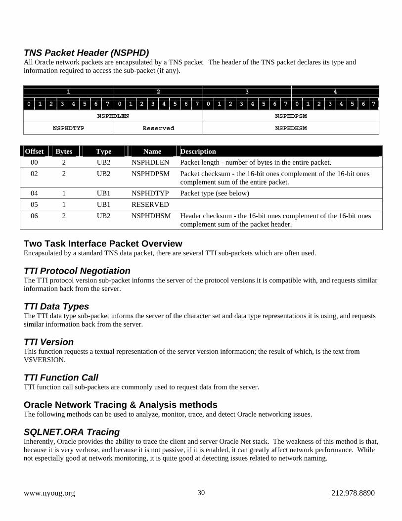
TNS Packet Header (NSPHD) All Oracle network packets are encapsulated by a TNS packet. The header of the TNS packet declares its type and information required to access the sub-packet (if any).

1 2 3 4

0 1 2 3 4 5 6 7 0 1 2 3 4 5 6 7 0 1 2 3 4 5 6 7 0 1 2 3 4 5 6 7

NSPHDLEN NSPHDPSM

NSPHDTYP Reserved NSPHDHSM

Offset Bytes Type Name Description

00 2 UB2 NSPHDLEN Packet length - number of bytes in the entire packet. 02 2 UB2 NSPHDPSM Packet checksum - the 16-bit ones complement of the 16-bit ones

complement sum of the entire packet. 04 1 UB1 NSPHDTYP Packet type (see below) 05 1 UB1 RESERVED 06 2 UB2 NSPHDHSM Header checksum - the 16-bit ones complement of the 16-bit ones

complement sum of the packet header. Two Task Interface Packet Overview Encapsulated by a standard TNS data packet, there are several TTI sub-packets which are often used. TTI Protocol Negotiation The TTI protocol version sub-packet informs the server of the protocol versions it is compatible with, and requests similar information back from the server. TTI Data Types The TTI data type sub-packet informs the server of the character set and data type representations it is using, and requests similar information back from the server. TTI Version This function requests a textual representation of the server version information; the result of which, is the text from V$VERSION. TTI Function Call TTI function call sub-packets are commonly used to request data from the server. Oracle Network Tracing & Analysis methods The following methods can be used to analyze, monitor, trace, and detect Oracle networking issues. SQLNET.ORA Tracing Inherently, Oracle provides the ability to trace the client and server Oracle Net stack. The weakness of this method is that, because it is very verbose, and because it is not passive, if it is enabled, it can greatly affect network performance. While not especially good at network monitoring, it is quite good at detecting issues related to network naming.

www.nyoug.org 212.978.8890 30

Generic Network Monitoring Using utilities such as Wireshark, or operating system utilities like tcpdump, you can passively capture and analyze Oracle Ethernet traffic. The downside here is that these utilities are fairly generalized and are not able to dissect the most important Oracle TTI packets. Oracle-Specific Network Monitoring Using utilities designed specifically to monitor and analyze Oracle network traffic provides the best and most detailed data. The downside in this case is that, because Oracle's network protocol is proprietary, very few people have spent the time researching it enough to write useful utilities. As such, there are very few of these utilities available. Oracle Network Conversations The following are basic examples of Oracle network conversations. Connection Conversation The connection process consists of: • Client requests a connection to TNS entry ORCL. • Network Naming finds ORCL in TNSNAMES.ORA. • Client builds and sends a TNS Connect Packet (NSPTCN) to the listener. • The Listener responds with a TNS Resend (NSPTRS) or Redirect [to another port] (NSPTRD) packet. • Client acts accordingly. • Server responds with an Accept (NSPTAC) or Refuse (NSPTRF) packet • Client requests additional services (ANO)

• Authentication • Encryption • Data Integrity • Supervisor

Authentication Conversation After connection, the client requests authentication from the server using the following process: • Client & server negotiate protocol version • Client & server negotiate data types • Client sends server basic information

• User Name • Terminal Name

www.nyoug.org 212.978.8890 31

• Machine Name • Program Name • …

• Server responds with challenge/response… Query & Fetch Conversation After being authenticated, the client (generally) requests data as follows: • Open a cursor • Parse the query • Execute the query • Fetch the data • Cancel the cursor • Close the cursor SCAPE4O SCAPE4O, SQL Capture and Analysis by Passive Evaluation for Oracle, is a utility which passively captures Oracle TCP/IP packets and provides the user with a detailed analysis of Oracle connections, statistics, query activity, and relevant response times (http://www.oracle-internals.com/). Architecture SCAPE4O is a multi-threaded application based on libpcap which can capture and analyze data directly from the network or from a stored packet capture. Analysis In addition to dissecting TNS, SCAPE4O is able to collect the following data for each SQL query found over the wire: • Top 10 Queries (By Time/Transfers/etc)

• Counters for • INSERT • UPDATE • DELETE • SELECT • COMMIT • ROLLBACK • PL/SQL (Anonymous Blocks) • DDL

• Response Time Advice In addition to helping identify network-related issues, SCAPE4O can recommend whether a more optimal SDU could be set or whether the application fetching method could be improved. Reference Material • OSI Text—Significant portions of the OSI model description was taken from Wikipedia under the terms of the GNU

Free Documentation License. • TNS Packet Structures—The TNS packet header and structure definitions can be found in Note:1007807.6,

SQL*NET PACKET STRUCTURE: NS PACKET HEADER.

www.nyoug.org 212.978.8890 32

http://www.oracle-internals.com/

Similar Oracle-specific Network Monitoring Utilities The following are utilities I know of which are similar to SCAPE4O: • WireCache (http://www.wirecache.com/)— Transparent Database Accelerator and SQL Query Analyzer Generic Network Protocol Analyzers The following are good generic protocol analyzers: • Wireshark (http://www.wireshark.org/)—Transparent Database Accelerator and SQL Query Analyzer • Microsoft Network Monitor (http://support.microsoft.com/kb/933741/en-us)—Transparent Database Accelerator and

SQL Query Analyzer Other Oracle Wire-level Software If you’re looking for other software which uses Oracle’s wire-level protocol directly, the following is a list of ones I’m aware of: • DataDirect (http://www.datadirect.com/)—Well-known wire-level ODBC, JDBC, .NET drivers. • CoreLab (http://www.crlab.com/)—Wire-level OraDirect .NET driver and Oracle Class Library for C++. • OraCmd (http://www.withdata.com/)—A Windows-only alternative to SQL*Plus written in Delphi by Shiji Pan. Appendix A: Source Code Excerpts /* ------------------------------------------------------------------------- */ /* -------------------- Network Substrate Packet Types --------------------- */ /* * Network Substrate Packet Header */ struct nsphd { ub2 nsphdlen; /* Packet Length (in bytes) */ ub2 nsphdpsm; /* Packet Checksum */ ub1 nsphdtyp; /* Packet Type */ ub1 nsphdrsv; /* Reserved for Future Use? */ ub2 nsphdhsm; /* Packet Header Checksum */ }; typedef struct nsphd nsphd; /* * Network Substrate Connection Packet */ struct nspcn { ub2 nspcnvsn; /* Packet Version */ ub2 nspcnlov; /* Lowest Compatible Version */ ub2 nspcnopt; /* Supports Global Service Options */ ub2 nspcnsdu; /* Session Data Unit Size (in bytes) */ ub2 nspcntdu; /* Transport Data Unit Size (in bytes) */ ub2 nspcnntc; /* NT Protocol Characteristics */ ub2 nspcntna; /* Line Turnaround Value */ ub2 nspcnone; /* The number 1 in Host Byte Order */ ub2 nspcnlen; /* Length of Connect Data (in bytes) */ ub2 nspcnoff; /* Byte Offset to Connect Data */ ub2 nspcnmxc; /* Maximum Connect Data */ ub2 nspcnfl0; /* Connect Flags 0 */ ub2 nspcnfl1; /* Connect Flags 1 */ ub2 nspcndat; /* Connect Data */ }; typedef struct nspcn nspcn;

www.nyoug.org 212.978.8890 33

http://www.datadirect.com/

http://www.datadirect.com/

Rapid Development of Rich CRUD Internet Applications

Yakov Fain, Farata Systems

http://www.faratasystems.com

In this paper we’ll show you how to create a CRUD application using Clear Data Builder , a free Eclipse plugin by Farata Systems, Oracle or other DBMS, and BlazeDS, an open source server side component by Adobe. This recipe should take you less than fifteen minutes after all the “ingredients” are installed and configured. If you prefer to start with watching pre-recorded video of how this CRUD was cooked, you can download the screen cast in avi (6MB) format ( in this demo we’ve used another DBMS though). http://www.myflex.org/demos/CDB_blazeds_db2.avi Ingredients 1. Eclipse IDE for Java Developers: http://www.eclipse.org/downloads/ 2. Adobe Flex Builder 3 plugin version: http://www.flex.org 3. Adobe BlazeDS 3.0: http://opensource.adobe.com/wiki/display/blazeds/download+blazeds+3 4. Clear Data Builder 3.0 plugin for Eclipse from Farata Systems:

http://www.myflex.org/cleartoolkit/site.zip 5. Apache Tomcat 6.0 http://tomcat.apache.org/download-60.cgi 6. Oracle Database 10g Express Edition http://www.oracle.com/technology/products/database/xe/index.html Out of these ingredients only Flex Builder 3 is not free unless you are a student, faculty or are willing to cook it with a 60-day trial version. Preparing the Cooking Table 1. Eclipse JEE installation is as simple as unzipping it to a folder on your hard disk. This recipe requires JEE version of

Eclipse because we’ll be using nice Web tools that come with it. 2. Installing of the plugin version of Flex Builder 3 is also easy. Do not install the standalone version of Flex Builder.

Get the plugin by following the link by the text “Have Eclipse already installed…” on Flex Builder download site. 3. Register at www.myflex.org and get the license to Clear Data Builder (CDB) - it’s free. The version for Flex 2 was

and still is on sale, but CDB 3.0 will be offered at no charge. Download the CDB 3 beta version at http://www.myflex.or/beta/site.zip. Unzip it into any folder on your disk and install CDB plugin by selecting Eclipse menu Help | Software Updates | Find and Install. Select the radio button “Search for new features to install”. Press the button New Local Site, give it a name (i.e. Local CDB) and point at the directory where you’ve unzipped the file site.zip. Install CDB license in Eclipse by using the Menu Window | Preferences |Flex |My Flex | License Management |Install license. The CDB license goes under the name daoflex, which was an open source predecessor of CDB.

4. Download the binary edition of BlazeDS , which is a relatively small (4Mb) zip file. Just unzip it into some folder, say in c:\blazeds like I did.

www.nyoug.org 212.978.8890 34

http://www.faratasystems.com/

http://www.myflex.org/demos/CDB_blazeds_db2.avi

http://www.myflex.org/demos/CDB_blazeds_db2.avi

http://www.eclipse.org/downloads/

http://www.flex.org/

http://opensource.adobe.com/wiki/display/blazeds/download+blazeds+3

http://www.myflex.org/cleartoolkit/site.zip

http://tomcat.apache.org/download-60.cgi

http://www.oracle.com/technology/products/database/xe/index.html

http://www.myflex.org/

http://www.myflex.or/beta/site.zip

To run this example, we JDK (not JRE) 1.5 or later. Use Eclipse menu Window | Preferences | Java | Installed JREs and point it to your JDK installation directory, for example:

5. Download Tomcat 6 - select Windows Service Installer from the Core Downloads section. Run the install accepting

all defaults. 6. The last preparation step is installing Oracle. During the install, we’ve entered sql as a password for the SYS account.

By default, Oracle installs HTTP Listener on port 8080. To avoid conflicts with another software using the same port (i.e. Tomcat), change this port as described at this page: http://download.oracle.com/docs/cd/B25329_01/doc/admin.102/b25107/network.htm#BHCBABJB By default, Oracle runs on port 1521 and the name of the sample database is HR. Enable the sample user hr with the password hr as described in the Oracle Getting Started manual located in your installation directory, for example, c:/oraclexe/app/oracle/doc/getting_started.htm.

Directions 1. Start Eclipse JEE and create a new instance of the Tomcat 6 server. Right-click in the tab Servers, select New,

Tomcat 6, and then click on Finish. 2. Create a new Dynamic Web Project in Eclipse using the menus File | New | Other | Web | Dynamic Web Project. Let’s

name the project RIA CRUD. Specify the Target Runtime (we use Apache Tomcat 6.0) in the Dynamic Web Project configuration screen:

www.nyoug.org 212.978.8890 35

http://download.oracle.com/docs/cd/B25329_01/doc/admin.102/b25107/network.htm#BHCBABJB

Press the button Next.

3. Select Clear Data Builder and Flex Web Project facets as shown below:

www.nyoug.org 212.978.8890 36

Press Next.

4. On the next screen, accept suggested RIA_CRUD as a context, WebContent as a content directory and src as a directory for the Java code. Press the button Next.

5. Now you need to specify that we are going to use BlazeDS and where your blazeds.war is located. We’ve entered C:\BlazeDS\blazeds.war in the Path to WAR file field. Press the button Next.

6. Finally, we need to specify that the application will be deployed under Tomcat, select and configure the database connection . Specify that you need Oracle database driver, give a name for the connection pool to be deployed, and enter the URL and user credentials as shown below.

www.nyoug.org 212.978.8890 37

We are planning build our CRUD application as the user hr connected to the sample database called HR . Do not forget to press the button Test Connection to ensure that you can connect with these credentials. To complete the project creation, press the button, Finish. 7. Create a new abstract Java class Employee (right-click on Java Resources), and enter com.farata as the package

name:

www.nyoug.org 212.978.8890 38

The code of the class Employee will look like this: package com.farata; public abstract class Employee { } It’s time for Clear Data Builder to chime in, but we need to prepare a method signature annotated (we use doclets) with our SQL statement that will bring the data to our CRUD application. We’ll need a couple of more lines of code to specify what’s the table to update and what’s the primary key there. The resulting class may look like: package com.farata; import java.util.List; /**

www.nyoug.org 212.978.8890 39

* @daoflex:webservice pool=jdbc/test */ public abstract class Employee { /** * @daoflex:sql * pool=jdbc/test * sql=::select * from EMPLOYEES * :: * transferType=EmployeeDTO[] * keyColumns=EMPLOYEE_ID * updateTable=EMPLOYEES */ public abstract List getEmployees(); } Double colons are used to specify the start and end of the SQL statement. But since it’s your first exposure to CDB, right-click inside the curlies in the class Employee, and you’ll see a Clear Data Builder’s menu.

Select Inject SQL sync template if you need a CRUD application or Inject SQL fill template if you are planning to create a read-only application. CDB will insert commented code that will help you to write similar code on your own. Now we can go to the Eclipse menu Project and perform the Clean operation , which will start the CDB code generation and build process. The Clean process invokes the ANT build script located under the folder daoflex.build. If you didn’t make any mistakes, expect to see BUILD SUCCESSFUL on Eclipse console. After this build, the Java DTO and data access classes were generated and deployed in our Tomcat servlet container. To see the Java code generated by CDB (if you care), switch to the Flex Builder perspective, click on a little triangle in the Flex Navigator view, select the Filters option and uncheck the “gen” checkbox as shown below:

www.nyoug.org 212.978.8890 40

Re-run the Ant script located in the daoflex.build directory to regenerate the code. The generated Java code is located under the folder .daoflex-temp\gen. If you do not see this folder immediately, refresh your Eclipse project by pressing F5. Technically, you do not need keep these source files as they are going to be jar’ed by CDB build process and deployed in the lib directory of your servlet container under WEB-INF\lib in the files daoflex-runtime.jar, services-generated.jar and services-original.jar. For the client side, CDB has generated the EmployeeDTO.as, an ActionScript peer of the generated EmployeeDTO.java. Clear Data Builder also generates a number of test Flex applications, which can be used as the front end of our RIA CRUD application. In a minute, we’ll use the one of them applications called Employee_getEmployees_GridTest.mxml. But first, we need to add your project to Tomcat server (open the Server view using the menu Window | Show View | Others |Server) . Right click on the line with Tomcat Server, select Add or Remove projects, and add the project RIA CRUD to the Configured projects panel.

Since Eclipse sometime behaves unpredictably during deployment of Web applications, we found a little hack to ensure that it works all the time - in the Flex perspective, open the configuration file org.eclipse.wst.common.components in the .settings folder, add somewhere a space character and re-save it. Start the server by using its right-click menu.

In Flex Perspective copy the reference implementation of the Flex client – the file file Employee_getEmployees_GridTest.mxml - from test.rpc.com.farata to flex_src directory, set it as a default application, right-click and run it as Flex application.

www.nyoug.org 212.978.8890 41

The basic RIA CRUD application is ready and Flex screen has been populated by the Java code with the data retrieved from the Oracle sample database called HR! To test the database updates, modify, say the last name of an employee. After you tab out of the last name field, the button Commit becomes enabled, and you’ll be able to apply your changes to the database. The button Fill on the screen above is used for data retrieval from the server side. The Add button is for adding new data. The button Remove becomes enabled when you select a row in the data grid. The source code of our RIA CRUD application is available, and you can use it as a foundation of your future project just add the required components. The server-side code is deployed under Tomcat server, and the relevant classes are located under the folder WebContent in your project. While generating this project, CDB has added a library component.swc to the build path. It contains the class library created by Farata Systems, which includes a number of handy components that enhance standard controls of Flex framework and a number of classes simplifying communication with the database layer. This class library is non-intrusive . It allows you to mix and match original Flex components with the ones that come with Flex framework. The difference between theriabook and all other Flex frameworks is that

a) it’s not a framework but a class library b) while other frameworks require you to add some extra code to your application, theriabook makes your codebase

smaller. For example, the following auto-generated code from Employee_getEmployees_GridTest.mxml uses an object DataCollection from theriabook, which is nothing else but a subclass of Flex class ArrayCollection. Look at the code in the onCreationComplete() function below. DataCollection is a smart data-aware class that combines the functionality of

www.nyoug.org 212.978.8890 42

Flex ArrayCollection, RemoteObject and some functionality of the Data Management Services that are available in LiveCycle Data Services. Just set the destination and the method to call, and call it’s methods fill() or sync(). No need to define the RemoteObject with result and fault handlers, no server-side configuration is required. <mx:Button label="Fill" click="fill_onClick()"/> <mx:Button label="Remove" click="collection.removeItemAt(dg.selectedIndex)" enabled="{dg.selectedIndex != -1}"/> <mx:Button label="Add" click="addItemAt(Math.max(0,dg.selectedIndex+1)) "/> <mx:Button label="Commit" click="collection.sync()" enabled="{collection.commitRequired}"/> … import com.theriabook.rpc.remoting.*; import com.theriabook.collections.DataCollection; import mx.collections.ArrayCollection; import mx.controls.dataGridClasses.DataGridColumn; import mx.events.CollectionEvent; import mx.formatters.DateFormatter; import com.farata.dto.EmployeeDTO; [Bindable] public var collection:DataCollection ; [Bindable] private var log : ArrayCollection; private function onCreationComplete() : void { collection = new DataCollection(); collection.destina "com.farata.Employee"; tion= collection.method="getEmployees"; //getEmployees_sync is the default for collection.syncMethod log = new ArrayCollection(); collection.addEventListener( CollectionEvent.COLLECTION_CHANGE, logEvent); collection.addEventListener("fault", logEvent); fill_onClick(); } private function fill_onClick():void { collection.fill(); } private function addItemAt(position:int):void { var item:EmployeeDTO = new EmployeeDTO(); collection.addItemAt(item, position); dg.selectedIndex = position; } private function logEvent(evt:Event):void { if (evt.type=="fault") { logger.error(evt["fault"]["faultString"]); } else { if (evt.type=="collectionChange") { logger.debug(evt["type"] + " " + evt["kind"]); } else { logger.debug(evt["type"]); } } }

www.nyoug.org 212.978.8890 43

Even though this code was auto-generated, nothing stops you from modifying it to your liking. CDB and our component library gives your project a jump start and the resulting code base is small – the Employee_getEmployees_GridTest.mxml is only about 90 lines of code, which includes 10 empty lines and the code for logging! The other freebee that CDB gives you is an automated ANT process of building and deploying your project both on the client and the server. You do not need to worry about creating compatible Java and ActionSript DTO objects. If the structure of the result set of the server side data is changing, just change the SQL statement in your Java abstract class and re-run the daoflex-build.xml. Clear Data Builder can be used either independently or as a part of Clear Toolkit 3.0 - a set of components, code generators, and plugins created by software engineers of Farata Systems that we were using internally in multiple Flex enterprise projects. In September of 2008, we’ll release its beta version. This toolkit will be available free of charge. Here’s what’s included in Clear Toolkit:

Components library is an swc file that includes a number of enhanced Flex components like Datagrid, ComboBox et al. Clear Data Builder 3.0 is an Eclipse plugin that allows to generate CRUD applications for BlazeDS or LCDS based on an SQL statement or a Java data value object. DTO2Fx is a utility that automatically generates proper ActionScript classes based on their Java peers. Log4Fx is an advanced logger (Eclipse plugin) that is built on top of Flex logging API but automates and make the logging process more flexible and user friendly. Fx2Ant is a generator of optimized ANT build scripts for your Flex Builder projects. ClearBI 3.0 is a Web reporter for smaller businesses. It includes an AIR-based report designer and flexible report generator that can be used by IT personnel as well as end users. Clear Toolkit is not an architectural framework. It consists of a set of components that extend Flex framework and tools built on top of these components that substantially increase productivity of the enterprise Flex developers. Each of these components can be used independently when needed. Consider Clear Toolkit (www.myflex.org ) for your next Flex-Java-Oracle project.

www.nyoug.org 212.978.8890 44

http://www.myflex.org/

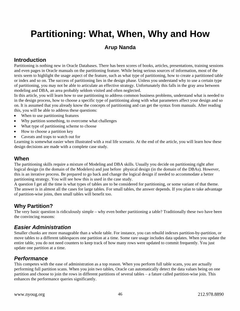
Partitioning: What, When, Why and How

Arup Nanda

Introduction Partitioning is nothing new in Oracle Databases. There has been scores of books, articles, presentations, training sessions and even pages in Oracle manuals on the partitioning feature. While being serious sources of information, most of the texts seem to highlight the usage aspect of the feature, such as what type of partitioning, how to create a partitioned table or index and so on. The success of partitioning lies in the design phase. Unless you understand why to use a certain type of partitioning, you may not be able to articulate an effective strategy. Unfortunately this falls in the gray area between modeling and DBA, an area probably seldom visited and often neglected. In this article, you will learn how to use partitioning to address common business problems, understand what is needed to in the design process, how to choose a specific type of partitioning along with what parameters affect your design and so on. It is assumed that you already know the concepts of partitioning and can get the syntax from manuals. After reading this, you will be able to address these questions: • When to use partitioning features • Why partition something, to overcome what challenges • What type of partitioning scheme to choose • How to choose a partition key • Caveats and traps to watch out for Learning is somewhat easier when illustrated with a real life scenario. At the end of the article, you will learn how these design decisions are made with a complete case study. When The partitioning skills require a mixture of Modeling and DBA skills. Usually you decide on partitioning right after logical design (in the domain of the Modelers) and just before physical design (in the domain of the DBAs). However, this is an iterative process. Be prepared to go back and change the logical design if needed to accommodate a better partitioning strategy. You will see how this is used in the case study. A question I get all the time is what types of tables are to be considered for partitioning, or some variant of that theme. The answer is in almost all the cases for large tables. For small tables, the answer depends. If you plan to take advantage of partition-wise joins, then small tables will benefit too. Why Partition? The very basic question is ridiculously simple – why even bother partitioning a table? Traditionally these two have been the convincing reasons: Easier Administration Smaller chunks are more manageable than a whole table. For instance, you can rebuild indexes partition-by-partition, or move tables to a different tablespaces one partition at a time. Some rare usage includes data updates. When you update the entire table, you do not need counters to keep track of how many rows were updated to commit frequently. You just update one partition at a time. Performance This competes with the ease of administration as a top reason. When you perform full table scans, you are actually performing full partition scans. When you join two tables, Oracle can automatically detect the data values being on one partition and choose to join the rows in different partitions of several tables – a fature called partition-wise join. This enhances the performance queries significantly.

www.nyoug.org 212.978.8890 46

Other lesser know performance enhancing features come from reduced latching. Partitioning makes several segments out of a single table. When the table is accessed, the segments could potentially be on multiple cache buffer chains, making fewer demands on the latch allocation. Hot Indexes Consider an index on some sort of sequential number – a monotonically increasing number. Since the numbers are added incrementally, a handful of leaf blocks may experience contention, making the index hot. Over period of time, the hot portion moves to a different part of the index. To prevent this from happening, one option is to create a hash partitioned index. Note, the table may or may not be partitioned; but the index could be – that’s the beauty of hash partitioned index, introduced in Oracle 10g R2. Here is an example of how it is created on a table called RES. create index IN_RES_01 on RES (RES_ID) global partition by hash (RES_ID) partitions 8 In this example the table RES is un-partitioned; while index is partitioned. Also, note the use of the clause “global”. But this table is not partitioned; so global shouldn’t apply to the index. Actually, it does. The global clause can also be used on partitioned indexes which are on unpartitioned tables. This creates multiple segments for the same index, forcing index blocks to be spread on many branches and therefore reducing the concentration of access on a single area of the index, reducing cache buffer chain related waits. Since the index is now partitioned, it can be rebuilt partition-by-partition: ALTER INDEX IN_RES_01 REBUILD PARTITION <PARTNAME>; It can be moved to a different tablespace, renamed and so on, as you can with a regularly partitioned index. More Important Causes The previous two causes, while important, are not the only ones to be considered in designing partitioning. You have to consider more important causes. Data Purging Purging data is a common activity in pretty much any database. Traditional methods of purge rely on deleting rows, using the DELETE command. Of course, TRUNCATE command can be used to delete the whole table; but purge is hardly ever for the entire table. DELETEs are very expensive operations; they generate a large amount of REDO and UNDO data. To prevent running out of undo space, you may resort to frequent commits, which stress the I/O subsystem since it forces a log buffer flush. On the other hand, partition drops are practically free. All you have to do is to issue a ALTER TABLE TableName DROP PARTITION P1 and the partition is gone – with minimal undo and redo. The local indexes need not be rebuilt after the drop; but global indexes will need to be. From Oracle 9i onwards, you can use UPDATE GLOBAL INDEXES clause to automatically update the global indexes during partition drop. Archival A part of the purge process may be archival. Before dropping the data, you may want to store the data somewhere else. For instance, you are deleting some sales data for April 2008; but you want to move them to a different table for future analysis. The usual approach is issuing INSERT INTO ARCHIVAL TABLE SELECT * FROM MAIN TABLE statement.

www.nyoug.org 212.978.8890 47

However, INSERT is expensive – it generates a lot of undo and redo. You can reduce it somewhat by using the /*+ APPEND */ but you can’t avoid the massive selection from the table. This is where the power of partition exchange comes in. All you do is to convert the partition to a standalone table. In line with the example shown above, you will need to create an empty table called TEMP – the same structure as the SALES table; but not partitioned. Create all the indexes as well. After the creation, issue the following: ALTER TABLE SALES EXCHANGE PARTITION APR08 WITH TABLE TEMP INCLUDING INDEXES This makes the data in the former partition available in TEMP and the partition empty. At this time, you can drop the partition APR08. The table TEMP can be exchanged with the partition APR08 of an archival table; or just renamed. During partition exchange, local indexes need not be rebuilt. Global indexes will need to be rebuilt; but can be automatically maintained if the UPDATE GLOBAL INDEXES clause is given. This is the fastest, least expensive and the preferred approach for archival. Materialized Views Refreshes You should already be familiar with Materialized Views, which are results of queries stored as segments, just like tables. The MV stores the data; not maintain it. So, it needs to be refreshed from time to time to make the data current. Traditionally, the approach to refresh the MV is calling the procedure REFRESH in the DBMS_MVIEW package. There is nothing wrong with the approach; but it locks the entire MV until the refresh is complete. Also, the data is inserted using INSERT /*+ APPEND */ statement, which stresses the I/O subsystem. Another approach is possible if the MV is partitioned properly. If done right, only a few partitions of the MV will need to be refreshed, not all. For instance, suppose you have an MV for Sales data partitioned monthly. Most likely the partition for a previous period is not going to change if you refresh it, as the base table data won’t have changed. Most likely only the last month’s partition needs to be refreshed. However, instead of refreshing, you can use the Partition Exchange trick. Fist you create a temp table structurally identical to the MV but not partitioned, along with indexes, etc. You populate this temp table with the data from base tables. Once done, you can issue ALTER TABLE MV1 EXCHANGE PARTITION SEP08 WITH TABLE TEMP UPDATE ALL INDEXES which updates the data dictionary to show the new data. The most time consuming process is building the temp table, but during the whole time the MV remains available. Backup Efficiency When a tablespace is made read-only, it does not change and therefore needs only one backup. RMAN can skip it in backup if instructed so. It is particularly useful in DW databases which are quite large and data is mostly read only. Skipping tablespaces in backup reduces CPU cycles and disk space. A tablespace can be read only when all partitions in them can be considered unchangeable. Partitioning allows you to declare something read only. When that requirement is satisfied, you can make the tablespace read only by issuing ALTER TABLESPACE Y08M09 READ ONLY;

Data Transfer When you move data from one database to the other, what are the normal approaches? The traditional approach is issuing the statement INSERT INTO TARGET SELECT * FROM SOURCE@DBLINK or something similar. This approach, while works is fraught with problems. First, it generates redo and undo (which can be reduced by the APPEND hint). Next, a lot of data is transferred across the network. If you are moving the data from the entire tablespace, you can use the Transportable Tablespace approach. First, make the tablespace read only. Then copy the datafile to the new server. Finally "Plug in" the file as a new tablespace into the target database. You can do this even when the platforms of the databases are different, as well. For a complete discussion and approach, refer to my Oracle Magazine article http://www.oracle.com/technology/oramag/oracle/04-sep/o54data.html.

www.nyoug.org 212.978.8890 48

http://www.oracle.com/technology/oramag/oracle/04-sep/o54data.html

Information Lifecycle Management When data is accessed less frequently, that can be moved to a slower and cheaper storage, e.g. on EMC platforms from DMX to Clariion or SATA. You can do this in two different ways: (A) Partition Move First, create a tablespace called, say, ARC_TS on cheaper disks. Once created, move the partition to that tablespace using ALTER TABLE TableName MOVE PARTITION Y07M08 TABLESPACE ARC_TS. During this process, the users can select from the partition; but not update it. (B) ASM Approach While the tablespace approach is the easiest, it may not work in some cases where you can’t afford to have a downtime for updates. If your datafiles are on ASM, you may employ another approach: ALTER DISKGROUP DROP DISK CostlyDisk ADD DISK CheapDisk; This operation is completely online; the updates can continue when this is going on. The performance is somewhat impacted due to the rebalance operation; but that may be tolerable if the asm_power_limit is set to a very low value such as 1. How to Decide Now that you learned what normal operations are possible and enhanced through partitioning, you should choose the feature that is important to you. This is the most important part of the process – understand the objectives clearly. Since there are multiple objectives, list them in the order of importance. Here is an example: • Data Purging • Data Archival • Performance • Improving Backups • Data Movement • Materialized View Refreshes • Ease of Administration • Information Lifecycle Management Now that you assigned priorities, you choose the partitioning approach that allows you to accomplish the maximum number of objectives. In the process of design, you might find that some objectives run counter to the others. In that case, choose the design that satisfies the higher priority objective, or more number of objectives. Case Study To help understand this design process, let’s see how decisions are made in real life scenarios. Our story unfolds in a fictitious large hotel company. Please note, the company is entirely fictional; any resemblance to real or perceived entities is purely coincidental. Background Guests make reservations for hotel rooms, for one or more number of nights. These reservations are always made for future dates, obviously. When guests check out of the hotel, another table CHECKOUTS is populated with details. When guests buy something or spend money such as order room service or buy a movie, records are created in a table called TRANSACTIONS. There is a concept of a folio. A folio is like a file folder for a guest and all the information on the guests stay goes in there. When a guest checks in, a record gets created in the FOLIOS table. This record gets updated when the guest checks out.

www.nyoug.org 212.978.8890 49

Partition Type To understand the design process, let’s eavesdrop on the conversation between the DBA and the Data Modeler. Here is a summarized transcript of questions asked by the DBA and answered by the Modeler. Q: How will the tables be purged? A: Reservations are deleted 3 months after they are past. They are not deleted when cancelled. Checkouts are deleted after 18 months. Based on the above answer, the DBA takes the preliminary decision. Since the deletion strategy is based on time, Range Partitioning is the choice with one partition per month. Partition Column Since deletion is based on RES_DT and CK_DT, those columns were chosen as partitioning key for the respective tables. create table reservations (…) partition by range (res_dt) ( partition Y08M02 values less than (to_date('2008-03-01','yyyy-mm-dd')), partition PMAX values less than (MAXVALUE) ) Here we have chosen a default partition PMAX to hold rows that go beyond the boundary of the maximum value. Access Patterns Next, we want to know more about how the partitions are going to be accessed. The DBA’s question and Modeler’s answer continues. Q: Will checkout records within last 18 months be uniformly accessed? A: No. Data within the most recent 3 months is heavily accessed; 4-9 months is lightly accessed; 9+ months is rarely accessed. Based on the above response, we decide to use Information Lifecycle Management to save storage cost. Essentially, we plan to somehow place the most recent 3 months data on highest speed disks and so on. Access Types To achieve the objectives of the backup efficiency, we need to know if we can make the tablespace read only. Q: Is it possible that data in past months can change in CHECKOUTS? A: Yes, to make adjustments. Q: How likely that it will change? A: Infrequent; but it does happen usually within 3 months. 3+ months: very rare. Q: How about Reservations? A: They can change any time for the future; but they don’t change for past records. This is a little tricky for us. Essentially, none of the records of CHECKOUTS can be made read-only, we can’t make the tablespace read only as well. This affects the Information Lifecycle Management decision as well. So, we put on our negotiator hat. We ask the question: what if we make it read only and if needed we will make it read write? But the application must be tolerant to the error as a result of being read-only.

www.nyoug.org 212.978.8890 50

After a few rounds of discussions, we decided on a common ground – we will keep last three months of data read write; but make everything else read only. If needed, we can make it read write, but with a DBA’s intervention. This decision not only improves the backup, but helps the ILM objective as well. Design: 1st Pass Now that we got all the answers, we get down to the design. Fig 1 shows the first pass of our design of the tables. The Primary Keys are shown by key icons, foreign keys by FK and partitioning keys are shown by the Part icon before the column name. The portioning keys are placed based on our initial design. Figure 1 Design: 1st Pass Design: 2nd Pass The first pass assumes we partition month-wise. There is a huge problem. The TRANSACTIONS table, which has a many-to-one relationship with FOLIOS table, has a different partitioning key – TRANS_DT – than its parent – FOLIO_DT. There is no FOLIO_DT column in the child table. So, when you join the table, which happens all the time, you can’t really take advantage of partition-wise joins. So, what can you do? The easiest thing to do is to add a column called FOLIO_DT in the TRANSACTION table. Note, this completely goes against the principles of normalization – recording data at only one place. But this is an example of where puritan design has to meet the reality head on and you have to make decisions beyond text book definitions of modeling. Fig 2 shows the modified design after the second pass.

Figure 2 Design: 2nd Pass

www.nyoug.org 212.978.8890 51

Design: 3rd Pass This solved the partition-wise join problem; but not others. Purge on CHECKOUTS, FOLIOS and TRANSACTIONS is based on CK_DT, not FOLIO_DT. FOLIO_DT is the date of creation of the record; CK_DT is updated at checkout. The difference could be months; so, purging can't be done on FOLIO_DT. We violated our first priority objective – data purge. So, we come up with a solution: make CK_DT the Partitioning Key, since that will be used to purge. This brought up another problem – the column CK_DT is not present in all the tables. Well, we have a solution as well: add CK_DT to other tables. Again, you saw how we tweaked the model to accomplish our partitioning objectives. After adding the column, we made that column the partitioning key. Fig 3 shows the design after the third pass of the design process. This was a key development in the design. Since the column CK_DT was on all the tables except RESERVATIONS, we can purge the tables in exactly same way.

Figure 3 Design: 3rd Pass

Design: 4th Pass While we solved the purging issue, we discovered some more issues as a result of the tweaked design. (1) The records of the table FOLIOS are created at check-in but the column CK_DT is updated at check-out. Since the column value could change, the record in FOLIOS may move to a different partition as a result of the update. (2) The column CK_DT will not be known at check-in; so the value will be NULL. This will make it go to the PMAX partition. Later when the record is updated, the record will move to the correct partition. The second problem is hard to ignore. It implies that all the records of the tables will always move, since the guests will checkout some day and the updates to the column will force row migration. The first problem is manifestation of the second; so if we solve the second, the first will automatically disappear. So, we made a decision to make CK_DT NOT NULL; instead it is set to tentative date. Since we know how many nights the guest will stay, we can calculate the tentative checkout date and we will populate that value in the CK_DT. Again, we made a step against puritanical design principles in favor of real life solutions. Our list of problems still has some entries. The TRANSACTIONS table may potentially have many rows; so updating CK_DT may impact negatively. Also, updating the CK_DT later may move a lot of rows across partitions; affecting performance even more. So, it may not be a good idea to introduce CK_DT in the TRANSACTION table. So, we made a decision to undo the decision we earlier; we removed CK_DT from TRANSACTIONS. Rather we partition on the TRANS_DT, as we decided earlier. For purging, we did some thinking. The TRANS_DT column value will always be less than or equal to the CK_DT, since there will be no transactions after the guest checks out. So, even though the the partitioning columns are different, we can safely say that when a partition is ready for dropping in FOLIOS, it will be ready in TRANSACTIONS as well. This works out well for us. This also leaves no room for row migrations across partitions. Fig 4 shows the design after the 4th pass.

www.nyoug.org 212.978.8890 52

Figure 4 Design: 4th Pass

Scenario Analysis One of the most important aspects of designing, including partitioning is thinking of several scenarios and how the design will hold up on each. Here we see different scenarios. The icons convey different meanings. I means a new row was created, U means the row was updated and M means the row was migrated to a different partition. Scenario #1 Guest makes a reservation on Aug 31st for Sep 30th for one night, so checking out tentatively on Oct 1st. Every table has an update date column (UPD_DT) that shows the date of update. He actually checks out on Oct 2nd.

Records Created: Table Part Key UPD_DT Partition

RESERVATIONS 09/30 08/31 Y08M09 I

Guest checks in on 9/30 FOLIOS 10/01 09/30 Y08M10 I

Checks out on Oct 2nd:

CHECKOUTS 10/02 10/02 Y08M10 I

TRANSACTIONS 10/02 10/02 Y08M10 I

FOLIOS 10/02 10/02 Y08M10 U

As you can see, all the records were created new. The only record to ever be updated is that of FOLIOS. But the record is not migrated from one partition to another. Design: 5th Pass While mulling over the design, we had a new thought: why not partition RESERVATIONS table by CK_DT as well? This action will make all the tables partitioned by the same column and the same way – the perfect nirvana for purging. When a guest checks out the reservations records are meaningless anyway. They can be queried with the same probability of the checkouts and folios; so it will be a boon for ILM and backup. Partition-wise joins will be super efficient, partition pruning between tables become a real possibility; and, most important of all, purging of tables will become much easier since we just have to drop one partition from each of the tables. So, we reached a decision to add a column CK_DT to the RESERVATIONS table and partition on that column. The new design is shown in Fig 5.

www.nyoug.org 212.978.8890 53

Figure 5 Design: 5th Pass

Scenario Analysis Let’s subject our design to some scenarios. First, let’s see how the Scenario #1 holds up in this new design. The guest makes reservation on Aug 31st for one night on Sep 30th; so checking out tentatively on Oct 1st. However, instead of checking out on the intended day, he decided to stay one more day and checks out on Oct 2nd.




Checks out on Oct 2nd:



RESERVATIONS 10/02 10/02 Y08M10 U

FOLIOS 10/02 10/02 Y08M10 U This shows that two tables will be updated; but there will be no migration across partition boundaries – so far so good. Scenario #2 It’s a modification of the Scenario #1. the guest checks out on Nov 1st, instead of Oct 1st.




Checks out on Nov 1st:


www.nyoug.org 212.978.8890 54


RESERVATIONS 11/01 11/01 Y08M10 M

FOLIOS 11/01 11/01 Y08M10 M

Consider the case carefully. The design reeks of two bad ideas in partitioning – row migration; but how prevalent is it? If you examine the scenario, you will notice that the only case the row migration will occur is when rows change months. When checkout date was changed from 10/1 to 10/2, the record was updated; but the row didn’t have to move as it was still in the Oct 08 partition. The row migration occurred in the second case where the month changed from October to November. How many times does that happen? Perhaps not too many; so this design is quite viable. Here you saw an example of how an iterative design approach was employed to get the best model for partitioning. In the process, we challenged some of the well established rules of relational design and made modifications to the logical design. This is all perfectly acceptable in a real life scenario and is vital for a resilient and effective design. New Column for Partitioning In the design, we added a column CK_DT to many tables. How do we populate it? There are two sources for populating it – applications and triggers. If the design is new and the coding has not begun, the apps can easily do it and in many cases preferred as it is guaranteed. If this is an established app, then it has to be modified to place the logic. In that case, the trigger approach may be easier. Non-Range Cases So far we have discussed only range partitioning cases. Let’s consider some other cases as well. Consider the GUESTS table, which is somewhat different. It has: • 500 million+ records • No purge requirement • No logical grouping of data. GUEST_ID is just a meaningless number • All dependent tables are accessed concurrently, e.g. GUESTS and ADDRESSES are joined by GUEST_ID So, No meaningful range partitions are possible for this table. This is a candidate for hash partitions, on GUEST_ID. We choose the number of partitions in such a way that each partition holds about 2 million records. The number of partitions must be a power of 2. So, we chose 256 as the number of partition. All dependent tables like ADDRESSES were also hash partitioned on (guest_id), same as the GUESTS table. This type of partitioning allows great flexibility in maintenance. Hotels Tables The table HOTELS holds the names of the hotels Several dependent tables – DESCRIPTIONS, AMENITIES, etc. – are all joined to HOTELS by HOTEL_ID column. Since HOTEL_ID varies from 1 to 500, could this be a candidate for Partitioning by LIST? To answer the question, let’s see the requirements for these tables. These are: • Very small • Do not have any regular purging need • Mostly static; akin to reference data • Not to be made read only; since programs update them regularly. So, we took a decision: not to partition these tables. Tablespace Decisions The partitions of a table can go to either individual tablespaces or all to the same tablespace. How do you decide what option to choose?

www.nyoug.org 212.978.8890 55

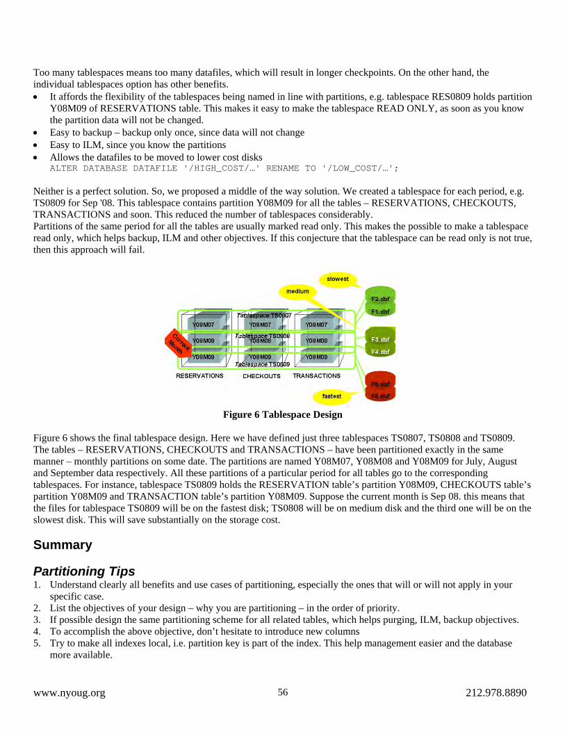
Too many tablespaces means too many datafiles, which will result in longer checkpoints. On the other hand, the individual tablespaces option has other benefits. • It affords the flexibility of the tablespaces being named in line with partitions, e.g. tablespace RES0809 holds partition

Y08M09 of RESERVATIONS table. This makes it easy to make the tablespace READ ONLY, as soon as you know the partition data will not be changed.

• Easy to backup – backup only once, since data will not change • Easy to ILM, since you know the partitions • Allows the datafiles to be moved to lower cost disks

ALTER DATABASE DATAFILE '/HIGH_COST/…' RENAME TO '/LOW_COST/…'; Neither is a perfect solution. So, we proposed a middle of the way solution. We created a tablespace for each period, e.g. TS0809 for Sep '08. This tablespace contains partition Y08M09 for all the tables – RESERVATIONS, CHECKOUTS, TRANSACTIONS and soon. This reduced the number of tablespaces considerably. Partitions of the same period for all the tables are usually marked read only. This makes the possible to make a tablespace read only, which helps backup, ILM and other objectives. If this conjecture that the tablespace can be read only is not true, then this approach will fail.

Figure 6 Tablespace Design

Figure 6 shows the final tablespace design. Here we have defined just three tablespaces TS0807, TS0808 and TS0809. The tables – RESERVATIONS, CHECKOUTS and TRANSACTIONS – have been partitioned exactly in the same manner – monthly partitions on some date. The partitions are named Y08M07, Y08M08 and Y08M09 for July, August and September data respectively. All these partitions of a particular period for all tables go to the corresponding tablespaces. For instance, tablespace TS0809 holds the RESERVATION table’s partition Y08M09, CHECKOUTS table’s partition Y08M09 and TRANSACTION table’s partition Y08M09. Suppose the current month is Sep 08. this means that the files for tablespace TS0809 will be on the fastest disk; TS0808 will be on medium disk and the third one will be on the slowest disk. This will save substantially on the storage cost. Summary Partitioning Tips 1. Understand clearly all benefits and use cases of partitioning, especially the ones that will or will not apply in your

specific case. 2. List the objectives of your design – why you are partitioning – in the order of priority. 3. If possible design the same partitioning scheme for all related tables, which helps purging, ILM, backup objectives. 4. To accomplish the above objective, don’t hesitate to introduce new columns 5. Try to make all indexes local, i.e. partition key is part of the index. This help management easier and the database

more available.

www.nyoug.org 212.978.8890 56

Tips for Choosing Part Key 1. If a column is updateable, it does not automatically mean it is not good for partitioning. 2. If partition ranges are wide enough, row movement across partitions is less likely 3. Row movement may not be that terrible, compared to the benefits of partitioning in general; so don’t discard a

partitioning scheme just because row movement is possible Oracle 11g Enhancements Oracle Database 11g introduced many enhancements in the area of partitioning. Of several enhancements, two stand out as particularly worthy from a design perspective. Virtual Column Partitioning It allows you to define partitioning on a column that is virtual to the table, i.e. it is not stored in the table itself. Its value is computed every time it is accessed. You can define this column as a partitioning column. This could be very useful in some cases where a good partitioning column does not mean you have to make a schema modification. Reference Partitioning This feature allows you to define the same partitioning strategy on the child tables as the parent table, even if the columns are not present. For instance, in the case study you had to add the CK_DT to all the tables. In 11g, you didn’t have to. By defining a range partitioning as “by reference”, you allow Oracle to create the same partitions on a table as they are on parent table. This avoids unnecessary schema changes.

Your Ad Here!

Vendors, place your advertisement in the NYOUG Tech Journal. Let our members know you want to do business with them.

Ad Options Available: Full Page – Black/White or Color

Half-Page – B/W only

Sponsorships: General Meeting – Primary and Secondary Special Interest Group

Journal Ad only Most sponsorship packages include color and/or black/white ads.

www.nyoug.org 212.978.8890 57

DW/BI - Design Philosophies, Accelerators, BI Case Study

Shyam Varan Nath [email protected]

Forrest Snowden [email protected]

Introduction Business Intelligence projects are rarely a trivial affair and unless done right have a high chance of failure. What can we do to reduce these risks upfront? Invest in the strategy; develop the BI strategy, or the vision for the organization, before jumping into the BIDW project. It is very tempting to be “agile” and “deliver” something in 90 days to the end users. However, the success of the BI project for the organization is not the first set of reports delivered in “iteration 1,” rather how it ties to the goals and strategic vision of the organization. It other words how business can drive the IT to get the right BIDW solution for the organization. Let’s start with a familiar example, where the end user interacts with a BI solution from a large organization, on a day-to-day basis. It’s Amazon, when we try to buy a book and put it in our shopping cart, the system comes up with recommendations for similar books and often the customer ends up buying if the recommendation makes sense. As a result of this BI solution in place, Amazon ends up in “up-selling” to the customer in the “window of opportunity” presented by the buyer. This is one example of a BI solution where the data warehouse provides the analytical information for data mining (market basket analysis) to be performed in near-real time and then interact with the operational system to fetch the books in stock as recommendations. You can experience similar use of analytics at Netflix. Do you think it is possible to deploy such successful BI projects, without talking time to develop the vision around it, or take the 10,000 ft view of the BI landscape in the organization? BI Accelerators Once the vision or the BI strategy is created, how do we ensure the success of the execution and deployment of a massive project? Its human nature to learn from mistakes but the mistakes need not be committed by us. When we travel from place A to place B, we follow a map, someone who has “been there done that” created the map for others to use it. It prevents us to stumble upon the destination, rather than move towards it in a definite way. Likewise, BI accelerators have been created by others who are more experienced in the domain and have “field tested” the process/product. Like a map, we can take advantage to reach to point B, which could be a final or intermediate phase of our BI implementation. This is not a new concept, if you are a Java programmer; you are used to reference architectures or design patterns. BI Accelerator is a set of processes, tools, templates with accompanying methodology to allow jumpstart in a BI project. The below visual, represents the cost and adaptability of a custom v/s BI accelerator-based project. We will look at more details of the same in the following sections. Now before, we dive into the use of a BI accelerator for the retail industry, let’s develop some level of understanding of the retail industry dynamics, specifically.

www.nyoug.org 212.978.8890 58



Fig 1 Custom Project v/s Use of BI Accelerators (packaged analytics)

Overview of Retail Industry Retail industry is part of our daily lives, starting from grocery stores to gas station to a clothing store – Wal-Mart to Shell to JC Penny, the list goes on and on. “Retail” means the selling of goods directly to customers. By definition it eliminates the wholesalers, so the vendors and suppliers to Wal-Mart are not retailers. Hence, the division of Proctor and Gamble what supplies to the Bentonville, AK based retail giant is not a retailer. Some of the common problems for retailers are loss prevention (check out what does a “sweet-heart deal” mean), customer retention, sales seasonal variations, over-stocking or under supply etc. Our goal here is to look at areas that can be addressed by Business Intelligence for the Retailers. If we find a good match between retail industry’s common problems and BI based solution, then we have passed the “business need” criteria for a BI project. The retail BI services market is about $175 million per year for USA. The retail market dynamics is forcing retailers to better understand customer demand, loyalty, retention and optimize the merchandise performance and profitability. The cost of accessing and analyzing their disparate data is one of the largest economic hurdle in this endeavor as shown in the below visual.

www.nyoug.org 212.978.8890 59

Fig 2 Strategic Software Investments Areas in 2008 to 2010

Let us now look at the BI maturity model. We can think of this as analogous to Maslow’s Hierarchy in the Theory of Human Motivation. The next step can only be “desired” if the former need is met. BI adoption is widespread across all sizes of retailers. Tier 1 retailers (with revenue>$1 billion) are looking for ways to move from “Anticipating” to “Collaborating”. Whereas, Tier 2 and 3 retailers (revenue <$1 Billion) are trying to move from “Reacting” to “Anticipating.”

Fig 3 BI Maturity Model

The next steps will show how to blend the Retail BI Accelerator-based solution to the overall BI strategy of the organization to solve some of the issues for retailers discussed in this paper.

www.nyoug.org 212.978.8890 60

Fig 4 Retailer’s BI Strategy on the Corporate BI/IT Landscape

Typically, the first step to blend the Retail BI solution, to the organization landscape, is to start with the BI Maturity assessment of the organization. With a series of questions, carefully designed for each dimension of the BIDW maturity assessment, one can arrive at the maturity or readiness of the organization for any BI project. This helps to create the prioritized roadmap for BI projects in the organization. A retailer, just like any other complex organization, is also likely to have typical IT challenges such as multiple ERP or commercial software packages, multi-vendor operating systems and data bases and silos of data in the enterprise. It is important to be cognizant of these challenges and develop a strategy to resolve these in a planned manner to ensure that the Retail BI solution is successfully implemented. Retail Business Intelligence Accelerator (RBIA) RBIA is a combination of reference data model, analytical layer with embedded advanced analytics based on OLAP and data mining along with pre-packaged reports with the goal of delivering relevant and actionable insights to the end user in the retail industry. RBIA comes with an industry compliant (Association for Retail Technology Standards -ARTS) data model for the retail industry. This ensures a compliant database layer in third normal form that can interact with any retail OLTP system. It does require ETL to bring data from the source system in the retailer’s organization. However, the target for the ETL is standardized. The internal ETL jobs based on Oracle Warehouse Builder (OWB), help to populate the analytical layer. This is the dimensional model and organized into facts and dimensions. This dimensional model is used to populate the aggregated layer consisting of OLAP data and mining table repository (MTR) for data mining. This analytical layer is pre-defined, the OBIEE based BI layer with pre-built content works out of the box to provide the reports, metrics and dashboards relevant to the different subject areas of retail industry.

www.nyoug.org 212.978.8890 61

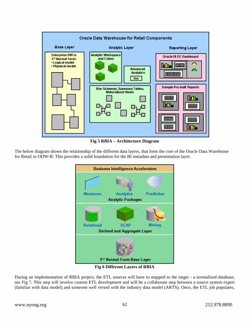
Fig 5 RBIA – Architecture Diagram

The below diagram shows the relationship of the different data layers, that form the core of the Oracle Data Warehouse for Retail or ODW-R. This provides a solid foundation for the BI metadata and presentation layer.

Fig 6 Different Layers of RBIA

During an implementation of RBIA project, the ETL sources will have to mapped to the target - a normalized database, see Fig 7. This step will involve custom ETL development and will be a collaborate step between a source system expert (familiar with data model) and someone well versed with the industry data model (ARTS). Once, the ETL job populates,

www.nyoug.org 212.978.8890 62

the base layer, the rest of the steps are out of box in RBIA. However, there will be some degree of changes desired to tune the end user reports and metrics to the specific retailer leading to minor changes in the base layer model. The ETL jobs to populate the analytics layer, provide the data for OBIEE to display to the end users as seen in the screen shot in Fig 8.

Fig 7 How RBIA/OWD-R Integrates with the Retailers ERP and Data Warehousing Environment

www.nyoug.org 212.978.8890 63

Fig 8 End user Experience (Retail Facilities Maintenance Trending)

The different business areas for retail industry are show below in Fig 9. These areas are represented in the OBIEE metadata layer and allow presentation layer to separate the functional areas from the end-user perspective. The security can be controlled using OBIEE to grant access to the specific areas of operation. Some of the questions the business users will try to ask in these areas will be: • How is my assortment selling in different regions of the country? • Who are my top customers in the category? What is the promotions/campaigns for best results? • Do I understand my gross margin return on space? • Are my inventory levels in line with the sales?

www.nyoug.org 212.978.8890 64

Fig 9 Major Business Areas for the Retailer

Install Overview & Optimization (Sizing, Platform, Partitioning, Compression, RAC) To implement RBIA, we have to install the Oracle RDBMS (EE) and OBIEE as the infrastructure layers. Database options like partitioning (to partition large fact tables) and advanced compression is useful for larger installations. Likewise, the use of RAC is advisable to allow horizontal scaling. Once the DB and the OBIEE software are installed, we can then install ODW-R software. This creates the database accounts for the base layer objects, the OLAP and data mining tables, creates the tables and other objects in them. Also it copies the prebuilt analytical content for OBIEE. Out of box there is a sample schema with data to help one test drive the RBIA. It will install about 650 tables, covering about 10 business areas. There are about 300 reports out of box with 15 OLAP cubes and 12 data mining reports. Retail Business Intelligence Accelerator is not to be confused with the term “BI Accelerator” often used in the industry to imply a piece of hardware used to accelerate the data warehouse. These are generally speaking, referred to as DW appliances. Oracle’s approach is to look for pre-optimized hardware configurations with the preferred hardware and OS vendors to improve the DW performance.

www.nyoug.org 212.978.8890 65

Fig 10 Advanced Analytics Areas for RBIA

Summary and Conclusion We looked at the challenges for the retail industry and how to use Retail specific BI solution for overcoming some of these to provide a competitive advantage. We looked at the need and use of Retail BI Accelerator to implement an end to end BI solution for a retailer by tying in the out of box components of RBIA to the source systems in the organization. This helps to reduce the time to see value for the retailer and avoids the full cycle development of a custom BIDW project. Such reusable solutions can be easily applied to a multitude of retailers to empower them to operate at higher levels of the BI maturity model. As the retail business is getting very competitive and the margins are shrinking, it’s time for the retailers to get BI savvy for quick wins.

www.nyoug.org 212.978.8890 66

ACCELERATE Your Back Office Processes! Eliminate Data Entry, Retrieve Documents in Seconds and Automate the

Approval and Exception Processing of Transactional Documents

• All Star provides solutions that automate business processes. Our solutions cap-ture inbound information (paper, fax, email, reports, eForm, EDI), extract perti-nent data, allow users to retrieve it in-stantly and automate the approval and exception processing of that information.

www.allstarss.com ACCELERATING Business Processes!

440 Smith Street Middletown, CT 06457 860 613 1500

Solutions

• Invoice Processing

• Expense Report Processing

• Sales Order Processing

• Credit Memo Processing

• Check Remittance Processing

• Invoice Delivery

• Mailroom Document Routing

Technology

• Workflow

• Information Capture

• Data Transformation

• Content and Document Management

• Paper and eForms Processing

• Enterprise Faxing

• ERP Report Output Management

All Star Software Systems is an Oracle Certified Partner specializ-ing in business process automa-tion. All Star is a full service organization who sells, implements and supports all of the software and hardware included in every solution. Our passion for success is only exceeded by the success of our implementations for our customers.

Storage Architectures for Oracle RAC

Matthew Zito, GridApp Systems [email protected]

Introduction Storage has always been of particular interest to the DBA. The mechanics of distributing data for optimal performance across a variety of different storage technologies and configurations has been the source of a great deal of DBA agita over the last 10-15 years. As storage has grown more complicated (snapshots, BCVs, different RAID levels, etc.) the challenge of understanding and optimizing databases for various storage environments has only increased. As an add-on technology, Oracle RAC increases this burden dramatically. This paper aims to provide a basic understanding of storage infrastructure for RAC, while discussing some of the specific benefits and disadvantages of various strategies. The vast majority of the content in this paper will be primarily applicable to Linux environments, with general applicability to UNIX, and little applicability to Windows RAC environments. In addition, there’s an expectation that the reader has a basic familiarity with RAC itself, as the core concepts will not be covered here. Background Oracle’s heavy marketing of RAC has been increasing the adoption rate since its introduction, especially when compared against its predecessor, Oracle Parallel Server. However, while RAC offers the possibility of all of the benefits listed above, there is a significant complexity curve associated with RAC at every tier. This is because clusters are, at their core, more complicated than running standalone systems, and running concurrent clusters, such as RAC, only introduce additional challenges above and beyond. This has placed an additional burden on the DBA, who has to not only deal with all of the application changes and performance optimizations that may be required in RAC environments, but also must deal with all of the infrastructure changes that are required as well. Over the last few years, though, it seems that while Oracle RAC internals may not be ideally understood by everyone, there is a general sense that there are “cookbooks” for rolling out RAC at a systems and network level. That is, enough people have gone down the road of building RAC clusters, that the process of configuring the operating system, clusterware, and network is significantly less terrifying than it might have been in the past. One notable exception to this, however, is in the area of storage. Storage continues to be a complex area for DBAs to manage in RAC environments, for a few reasons: • There is a complex matrix of rules for supported and working storage configurations • There is a multitude of storage technologies that may be utilized, each with particular benefits and limitations • RAC typically isn’t in a DBA’s background Let’s begin, then, by discussing some storage fundamentals. Storage Foundations Servers today communicate with storage arrays in one of two general methods based on mechanism of access, block, and file. Block-based storage is far and away the most common type of storage connected to database servers today. Standard block-based technologies include Fibre Channel, iSCSI, SCSI, and SATA. With block-based storage, the host “sees” one or more disk devices, often presented as Logical Unit Numbers (LUNs) on a single SCSI target. The host can interrogate those disks to identify sizes and layouts, read data, and write data. At a high level, this is all the system needs to do. In block-based storage, the storage is completely unaware of what is being written to the disks it is presenting to the hosts – it is simply responding to the commands with the appropriate response. Any intelligence about data layout for performance, locality, as well as metadata about relationships, modification times, or data protection needs to come from a higher level technology within the server.

www.nyoug.org 212.978.8890 68

File-based access is very common in IT generally, but more rare in database environments. The most common examples of file-based storage protocols are NFS and CIFS. With file-based protocols, the storage array itself exposes a set of semantics similar to a filesystem, with directories, attributes, metadata, authentication, etc. With file-based access, instead of simple read and write commands, the protocol dictates a wide set of operations, such as opening directories, reading them, locking files, etc. Block-based storage relies on a higher level technology to provide comparable functionality to file-based access – a filesystem being the most common example. In this way, the storage array can remain “dumb”, focusing purely on performance and availability, and the host server can handle all of the intelligence. It may be noted that we haven’t discussed the concepts of “SAN” or “NAS” yet because the lines between the two have been blurring over the past few years. Ten years ago, “SAN” meant a Fibre Channel network and its attached storage, and “NAS” meant an NFS array. Today, technologies such as iSCSI, where block storage is delivered over Ethernet, blur the line between the two concepts. Consequently, we’ll avoid them. Storage and RAC In RAC environments, there’s a requirement that all database instances running on servers in a RAC cluster have access to a shared set of storage. Any storage device, whether file or block-based, needs to be accessible by all nodes. This presents a number of problems right off the bat. First, it’s not as common a configuration, except for groups already using clustering solutions with shared disks, such as Veritas, and some storage administrators aren’t sure how to correctly configure block storage to be accessible by multiple nodes simultaneously. Even worse, not all storage vendors support these types of configurations. Second, traditional technologies are often not compatible with shared storage access. Concurrent access to a storage device from multiple nodes where there’s an expectation of consistency is a lot more complicated, and hence, many filesystems, NFS fileservers, etc. are simply not built to support that. Consequently, specialty storage technologies that are built for concurrent access, guaranteed writes, and atomic updates are required. Today, there are four general classes of RAC-suitable solutions for storage on RAC: raw devices, clustered filesystems, ASM, and NFS. Raw Devices Raw devices are the oldest solution to storage configurations for RAC. In fact, in the OPS days, they were a requirement. At a high level, raw devices are just bare disks, with no operating-system layer of intelligence atop them. Raw devices depend on the fact that Oracle already needs to know how to arbitrate writes between the nodes in the RAC cluster. This is because even if there was a smart filesystem in use that could arbitrate between the two different servers, it would still be possible for those servers to both write to the same block on disk at the same time, unless Oracle knew to coordinate that itself. But what, specifically, is a raw device? The exact details are different from operating system to operating system, but a raw device is a disk or partition (subset) of a disk where all I/O operations to that device bypass any OS-level caches or buffers and are delivered immediately to the driver subsystem. This allows for guaranteed writes, which is critical in RAC environments. Imagine, for example, if in a RAC environment one instance wrote a block to disk, was told by the OS that the block had been written when it had actually been queued for writing, and then the other instance immediately reads the block off of disk? Corruption, or at the very least, confusion ensues. Raw devices also offer very high performance, since there’s no intervening filesystem to add overhead or latency to the I/O operations. In effect, writing to raw devices is writing at the raw speed of the server to storage channel. In RAC environments, spfiles, OCR and voting files, password files, and of course datafiles can all be placed on raw devices. The binary installs for Oracle and the CRS can not be placed on raw devices. It would seem, then, that raw devices are the ideal solution for Oracle RAC. They are high performing with no additional moving parts in the process, and are single vendor. The reality, though, is more complicated. First of all, Oracle treats each raw device or raw partition as one big file – so one partition is needed for every datafile, dramatically increasing the complexity of the storage configuration. Second, because the server OS is unaware of how the database is using the various raw devices, there’s no way to get an accurate picture at an OS level of how much disk space is in use. While

www.nyoug.org 212.978.8890 69

DBAs may be accustomed to looking at the Oracle instance itself for utilization, systems and storage teams certainly are not, and raw devices may not work correctly with standard monitoring and capacity planning tools. Finally, backup and recovery solutions that do backups at an OS level are raw devices unaware as well, generally forcing the use of a backup solution that is integrated with the Oracle instance itself and leveraging RMAN. In the end, raw devices will eventually be phased out by Oracle. In Metalink note 578455.1, Oracle announces that starting in Oracle 12g, raw devices will no longer be supported. Oracle 12g is far enough in the future that current raw device don’t need to rush to migrate off of them, but it certainly does suggest that the next time a system is upgraded or migrated, removal of raw devices might be a good idea. Clustered Filesystems A clustered filesystem, or CFS, offers the most familiar environment for systems people and DBAs alike, since it perfectly resembles the traditional filesystems used in non-RAC environments, except that the same filesystem is mounted on all of the nodes in the RAC cluster. All of the standard commands and semantics needed for day-to-day administration are there – “df” works, archive logs can be deleted by hand, and backups can be run directly off of the file system. In addition, the clustered filesystem can often be used to store non-database files, such as trace files, alert logs, and even the Oracle CRS and database install itself. While Oracle supports having one shared install of binaries on a clustered filesystem that all of the nodes access, that configuration offers few advantages, and many disadvantages. The only defined advantages are the reduced disk utilization required, since an N-node cluster needed only 1 install of the various Oracle RAC components, and simplified patching and upgrades, since again, the various components needed to be upgraded in only one place. However, the associated disadvantages are that while a clustered install does save disk space, it requires leveraging the shared storage, which is often more expensive per megabyte than the local disks of the machine. It also creates a massive single point of failure: the loss of that one mount point or a patch apply gone wrong or a misfired rm command or a SAN issue relating to that one volume. Now all of the nodes are down, defeating one of the defined purposes of RAC. Some organizations work around that particular limitation by having a small number of shared installs. For example, in a four node RAC cluster, nodes 1 and 2 share one set of installs, while nodes 3 and 4 share a second set of installs. However, in the opinion of this author, this adds complexity without significantly mitigating the other disadvantages. It is far better to simply leverage the clustered filesystem for logs, datafiles, and other database filetypes. Clustered filesystems work in a very similar fashion to RAC itself. Each node participating in the clustered filesystem needs to have access to the disk devices, and daemons running on the nodes provide cluster synchronization, lock management, and fencing capabilities. Lock management is particularly important in clustered filesystems, as the filesystem metadata, things like access times, directory trees, and inode tables are shared data structures. Consequently, when a node is going to update the shared metadata, it needs to request a lock for that metadata, such that no other node is modifying that structure at that time. Fencing becomes important to ensure that a node that is not functioning correctly does not misbehave, or believe that the other nodes have gone down while it is still healthy, thus corrupting data on the filesystems. The specifics of how these various components are implemented vary, but as an example, some filesystems depend on the application itself to provide fencing, such as OCFS2, while other filesystems, such as Red Hat’s GFS, actually integrate with storage or power management to “hard fence” nodes by actually turning them off, or removing their access to the network or storage. There are a multitude of Oracle-supported cluster filesystems – an entire paper could be devoted to simply describing their differences and advantages, but there are a number of generalizations that can be made. One is that except for Linux, all of the clustered filesystem options are provided by a third-party vendor, such as Symantec/Veritas or IBM. This means bringing another vendor into the already-complex RAC stack. Along those lines, since a clustered filesystem has its own RAC cluster equivalent, two whole cluster stacks are required, one for the CFS, and one for RAC itself. This not only increase the operational complexity, but also the cost since the third-party solutions often have associated licenses that must be purchased. Third-party CFS options do offer good functionality, and the accompanying benefits of CFS configurations, but at a dollar cost and a complexity cost that may outweigh the benefits. On Linux, Oracle has written its own CFS, OCFS2 (Oracle Clustered Filesystem version 2). A vast improvement over its predecessor, OCFS, it is actually a general purpose clustered filesystem, though its primary use case is for Oracle datafiles. OCFS2 offers a lightweight cluster engine for lock management and fencing, and good performance for

www.nyoug.org 212.978.8890 70

database-type activities, such as simple block reads and writes. OCFS2 is free, and has even been accepted into the Linux mainline kernel, giving it a legitimacy that has eluded other Linux clustered filesystems. OCFS2 does have some limitations, however. It is not a volume manager, and consequently does not have the ability to have an OCFS2 filesystem span multiple physical disks. For organizations whose SAN admins provide them multiple disks of a fixed disk size, typically due to SAN array limitations, this creates a headache. If a DBA is only able to get 18GB disks presented from the SAN, a 180GB database would require 10 OCFS2 mountpoints, with the DBA having to manually distribute datafiles across them. This a hardly an ideal situation. Another limitation is growing filesystems – while some SAN arrays are able to grow devices online to increase the size, growing an OCFS2 filesystem requires it to be unmounted on all nodes in the cluster, effectively requiring a downtime. Oracle ASM Oracle ASM is Oracle’s attempt to bridge the gap between the limitations of raw devices, and the cost, complexity, and limitations of clustered filesystems. ASM is a striped down Oracle instance or RAC database that acts as a volume management layer for Oracle database-related files, such as redo logs, archive logs, and datafiles. ASM’s concept of volume management is very simplistic compared to “traditional” volume managers, due both to Oracle’s attempts to encourage people to simplify their Oracle database storage configurations and ASM’s specialization towards database environments. In ASM, disks are grouped together as named “disk groups”, which have a data protection level associated with them. Any data written to the disk group is distributed across the various disks in 1MB chunks based on the data protection rules. For example, a user might have a disk group called “+redo” that had four disks in it and was “high” protection. Every block of data written would be written to three of the four disks. There is also “normal” redundancy, which writes to two disks, and “external”, which writes to just one. The ASM instance itself keeps track of the maps where the data lives, and the configuration of the various disk groups. The database instances that are reading and writing data query, the ASM instance to discover the configurations of the disks, disk groups, and the data contained within, but all read/write operations themselves are sent directly to the disks. This removes ASM as a potential bottleneck for performance, though it does add a requirement that ASM is up for the database to be up. ASM also allows disks to be added to disk groups online, and data will automatically be evenly distributed across the new disks. The primary advantage of ASM over raw devices is that it removes the “one disk, one datafile” requirement while maintaining raw device performance levels. It also gives DBAs a filesystem-esque interface for creating datafiles, redo logs, etc. that are then mapped to the various raw devices in question. The ability to grow the ASM diskgroups online is also a dramatic advantage over OCFS2. Finally, ASM is cross-platform allowing multi-vendor environments to share a common solution for their database file storage. One of the major disadvantages of ASM is that since it can only store database files, raw devices or a CFS are still needed for the OCR, voting, spfiles, and password devices for the ASM instance and any database instances. There also needs to be local disk space on the server or a CFS for the database installs, dump locations, and any other non-database object. Another disadvantage is that just like raw devices, ASM configurations are invisible to the OS, forcing systems and storage teams to again look inside the database to attempt to determine utilized capacity. There is a command-line interface to ASM, asmcmd, that mitigates this to a certain degree, but it does not remove these objections completely. Oracle 11g offers a number of enhancements to ASM. One is that previously, when ASM was providing mirroring or disk redundancy, if a disk failed temporarily and then returned, Oracle would need to completely rebuild all of the data on that disk. This was not a huge issue in small environments, but when large disks, 100GB or more, were being used the rebuild could take days in some situations, during which the database was at risk for data loss. Another enhancement is the addition of the “sysasm” group, similar to the sysdba group, except targeted towards ASM. The sysasm group allows systems or storage administrators to have access to the ASM instance on a machine, without giving them access to the database instances for role and privilege separation purposes. It is fairly obvious that Oracle has bigger plans for ASM, and it is expected that future releases of Oracle will extend the ability of ASM to hold non-database files. This will continue to make Oracle ASM more broadly competitive as a storage option for database environments.

www.nyoug.org 212.978.8890 71

NFS Network File System (NFS) has had a bad rep among DBAs for years, generally dismissing NFS as slow and unreliable. DBAs instead focused on Fibre Channel as a storage platform, citing higher performance and better uptime as major reasons. NFS started to become a much more attractive option with RAC’s introduction, since it removed the whole question of CFS vs. raw devices (and later, ASM), and offloaded all of the heavy lifting to the storage array. In NFS environments, the NFS server or array effectively acts as a CFS, arbitrating access, locks, and metadata updates. However, since NFS is akin to a clustered filesystem, Oracle has certified only a small number of NFS server options, limiting vendor choice. NetApp and Oracle have the closest partnership on that front, but EMC, BlueArc, and HP all have certified NFS options. NFS in Oracle environments also got a shot in the arm with 11g, when Oracle introduced a cross-platform direct NFS client embedded in the database itself. While greeted with skepticism initially (“It took Linux years to get a decent NFS client, how could Oracle build one from scratch?”), performance and scalability metrics have been compelling, and it is expected that in the future, Oracle will offer even more NFS options. NFS may not be well-suited for extremely high-performance environments. If a database is saturating multiple Fibre Channel connections to large SAN storage arrays, it is unlikely that NFS will be able to keep up. NFS is also more expensive, per megabyte, than comparably sized Fibre Channel or iSCSI arrays. But when the cost and complexity of the CFS in SAN environments is factored in, along with the rich feature set provided by many of the NFS platforms, it becomes a more attractive option, and definitely one to be considered. A Recommended Configuration Over time and viewing many customer RAC environments, one configuration stands out as a manageable, scalable, high-performance storage configuration. This is only applicable to Linux, and would not apply generally to other OSes. In this configuration, the binary installs for the databases and CRS are on the local disks of the machine in a non-shared fashion, to reduce the cost burden of expensive SAN storage. Three OCFS2 mounts are created on different disks. The OCR, voting, database and ASM spfiles and passwd files, and optionally an archive log destination are striped across these three disks, providing redundancy in the event of any one disk failure. This cuts the number of block devices needed for these components down to three, and provides an easy way to stage scripts or other files that need to be accessible to multiple machines. Finally, ASM stores all of the datafiles, redo logs, and flash recovery areas to provide high performance storage, online scalability, and pooling of disk resources not typically available in raw device configurations. This configuration is not ideal for everyone, but it appears to be the best intersection of complexity, cost, and performance for Linux RAC environments. Conclusion Oracle RAC, while an exciting technology, dramatically increases the infrastructure complexity surrounding its configuration. Storage, network, and OS configuration all require special care and attention, but with storage, there is a particular concern due to the breadth of options available. Raw devices, NFS, CFS, and ASM all have particular advantages and disadvantages, and careful preparation and planning are advised for any organizations stepping into the world of RAC.

www.nyoug.org 212.978.8890 72

Control Complexity with Collections

Travis R. Rogers, Truppenbi LLC [email protected]

Intended Audience This paper is intended for individuals that have a basic understanding of Oracle databases, SQL and PL/SQL. The topics discussed are specific to Oracle and will be best understood and utilized by individuals with some hands-on experience. Scope The intent of this paper is to discuss the use of collections within the Oracle environment with a specific focus on how to apply this knowledge to standardize and simplify usage. This is by no stretch a thorough discussion of either managing the complexity of software development or of Oracle collections. One of the primary goals is to convince readers that collections are valuable tools in day-to-day PL/SQL tasks and to provide enough information to get started. Items to be discussed are:

1) Define PL/SQL Collections

2) Define Oracle Objects (collections).

3) Effects on the Database.

4) Debugging hints.

Please note that when discussing the history, motivation or intended focus of a feature the author has no inside information other than personal experience, data that is readily available in documentation or via other readily available sources. There are attempts to deduce the reasoning for the existence of some features but are not definitive statements of fact. As with anything that you read the author encourages you to approach this information with open minded and fair skepticism. If you feel anything is inaccurate or misrepresented, or if you would just like to express a different opinion, please feel free to address it to [email protected]. Is a PL/SQL Record a Collection? This really depends on your point of view but practically speaking a PL/SQL Record is more like the row of a table. It’s called a “PL/SQL Record” because it only exists in PL/SQL, has no permanent storage, can represent a single “row” or can represent multiple rows by declaring a [PL/SQL memory resident] table of records. In terms of other development languages it is like a struct but not an object. Even though it’s not a collection it will be discussed in this paper along with collections because they have similar histories and it is the collection and the record together that is most useful for non-trivial applications. It appears that Oracle also considers them similar or at least complementary since Oracle documentation always discusses collections and records together. Complexity I have been doing data focused software development for 17 years and in that time I’ve learned that it is hard to do it right but most people not involved in the nitty-gritty of the process believe that it is easy. Data geeks speak in terms of views, record sets, result sets and etc; but in effect are developing an API for use by others (report writers, GUI developers, analysts, automated tools and etc). As with any good API the complexity should be hidden as much as possible leaving clean and easy to use interfaces. Proper use of collections will help provide these interfaces. If 100 developers are given the same problem to solve how many solutions will be provided? I have never heard anyone answer this question (or others like it) with 1. That’s because there are so many possible ways to design a software solution that it is unlikely that any 2 will be exactly same. Unlike many I’ve heard discuss this issue I don’t believe that software development (or technology in general) is unique in this aspect. I think lawyers, accountants, architects and business owners often find different ways of achieving the same goal. An example of this is making money, it is a single

www.nyoug.org 212.978.8890 73


goal but there are a lot of different ways of achieving it with varying degrees of effort and success. I believe that this question may hint at one reason that technologists compare themselves to artists. People in all walks of life are compared to artists, the difference in my mind is that all artists can come to a result differently regardless of their talent level and this is true for most developers. However, only the best of most other professions are considered “artists”. The answers that go through your head from the three questions below should give you an idea of what I’m talking about. If 100 artists are asked to draw a circle, how many different versions will be provided? If 100 accountants are asked to add a list of numbers how many different methods will be used? If 100 developers are asked to write a “Hello World!” app how many versions will be provided? For the record, my answer to the original question (1 problem and 100 developers) is 54.

1) 5 developers will not have the necessary skills.

2) 15 developers will have the skills but will misunderstand the requirements.

3) 15 developers will be re-tasked by management prior to finishing the project.

4) 15 developers will have understood the requirements at the beginning but someone (management, architect or technically savvy business person) will have come along and confused them into delivering something else.

5) 46 developers will have achieved the goal in 46 different ways.

6) 4 developers will have done it 2 different ways each just to show off. Regardless of the answer or the underlying reasons, the fact that there are so many options, means that managing this complexity must be a high priority. About Performance 80/20 Rules of Application Performance 80/20 rules abound for about every topic that is more complex than how many licks it takes to get to the middle of a Tootsie Pop. Come to think of it there may be an 80/20 rule for that as well, something like; “80% of the Tootsie Pop’s consumed are bitten before the middle is reached and 20% of the time it is licks only.” The interesting thing is that while not accurate this “rule” is probably more true than false and can be used as a general guideline. The same goes for application performance, the need for or effort to attain “ultimate performance” (whatever that means) will vary from circumstance to circumstance. However, this too can be generalized by saying…

20% of the time ultimate performance MUST be achieved but 80% of the time decent performance is acceptable.

…plus…

20% of the effort is required to achieve decent performance while an additional 80% is required to achieve ultimate performance.

...and to continue the trend of generalizations…

There is a direct correlation between the effort required to deliver a requirement and the complexity of the solution.

www.nyoug.org 212.978.8890 74

As with the Tootsie Pop rule there is considerable truth in all of these, but more importantly, together they provide a picture that we can use to help guide the management of software complexity. A few years ago a team was struggling to meet some newly applied SLA’s. As part of a quick initial review it was determined that one data loading application was taking 1+ hrs and if it could run in 15 minutes or less it would solve the majority of the problems. A developer was tasked to make the modifications and 2 weeks later he delivered the changes with a minimal increase in complexity and a run time of 6-10 minutes. This same developer indicated that with “some more work” it could run in 3-5 minutes. After further discussion it was decided that “some more work” would be multiple weeks and would significantly increase the complexity of the application. Much to the chagrin of the developer it was decided that his time would be better spent elsewhere but if the need ever arose his suggestions would be implemented. The component ran successfully for several years. This situation showcases the understanding and application of the above ideas leading to success:

1) The change was identified in an initial (ie not overly detailed and expensive) review of the processes. 2) The change was made with minimal cost. 3) The component was relatively easy to maintain. 4) The component was relatively easy to use.

The purists and “techniacs” will argue that had the process been written for ultimate performance initially the change wouldn’t have been required at all. This is fair, but the reality is that prior to the change it had ran satisfactorily for several years (paying for itself and the changes many times) and barring the use of a crystal ball no one would have foreseen all the business circumstances requiring the change. Nor would anyone have been able to foresee the direction of the technology that allowed such a simple change. For example, the decision not to spend the extra time turned out to be correct as circumstances eventually made the component obsolete prior to needing it to run in half the time. Besides, incidental changes in technology allowed performance to increase without any extra cost (in other words the $ was spent for another reason and this component benefitted). The problem of complexity is amplified in the use of libraries and off the shelf software. Early versions of software normally have a specific focus and solve specific problem(s). In the case of Oracle the first versions didn’t have any special stored procedure language. At some point in the maturation process the core requirements of the majority user population are addressed (ie select * from emp) and additional features are added which are useful to smaller “fringe” user populations. Often these features overlap in purpose providing similar but slightly different implementations of the same thing. Most of the time the reason for these “different yet similar” implementations are due to performance characteristics (ie functions f_a() and f_b() do the same thing but f_a() is slightly faster but requires a lot of memory while f_b() is a little slower but requires very little memory). Features and options are good, but one unfortunate side affect of having so many options is that people often get overwhelmed and end up not using relevant features at all. Oracle has been around for a while now and it is easy to point to situations just like this…including collections and objects. Listen to the purists and techniacs and you’ll believe that every feature must be considered in every circumstance no matter what. There is no doubt we are responsible for understanding all the possibilities and using them when appropriate, but the ideas above indicate that appropriate rarely means “ultimate performance”. It is appropriate to use standard methods most of the time as long as they deliver the requirements. It is equally appropriate to use non-standard methods when necessary to meet the requirements. It is not appropriate to constantly change methods in vain attempts to always achieve the “ultimate” whatever. From this conversation we can glean some additional generalizations.

1) Use the 20% you need for 80% of your job and the other 80% only when necessary.

2) Don’t get overwhelmed by all the functionality that exists in order to support 20% of the requirements.

3) Understand the options enough to create standards.

4) Understand the options enough to know what is possible when the standards aren’t good enough. There is a very basic standard that is repeated ad nauseum by all Oracle experts that bears repeating before continuing on to discuss collections.

If you can do it via SQL then do it via SQL!

www.nyoug.org 212.978.8890 75

This is good but as with any other standard or generalization can be taken to ridiculous extremes like individual SQL statements three pages long or longer that are virtually incomprehensible. Collections – A History As was mentioned prior, the “maturing” of off-the-shelf software leads to the creation of many different options. Often it is easier to understand what exists now by looking at the history of the features. That is the way we will define Oracle collections. In the Beginning… In the very beginning there was no PL/SQL or any other stored procedure language in the Oracle database. When PL/SQL was added as an option there was no collection type, not even an array so there was no simple programmatic way store multiple of one or more types. Eventually two language components were added, the PL/SQL Table and the PL/SQL Record. PL/SQL Table In later versions the PL/SQL Table would also be referred to as an “Index By Table” and an “Associative Array”. This version only allowed the declaration using a single scalar datatype (number, char, varchar and etc.) and had to have an index of type binary_integer. This construct was different from a traditional array as it was unbounded (no max size needed to be specified) the index could be sparse (could be any number and didn’t need to be sequential) and the index could be negative. An example declaration is:

TYPE ex_tab IS TABLE OF VARCHAR2(200) INDEX BY BINARY_INTEGER;

Since the “INDEX BY” could only be a “BINARY_INTEGER” it seems wordy and unnecessary but Oracle had other plans for this construct and by enforcing the additional verbiage they eliminated later issues with backward compatibility. The “other plans” will be seen in a later version of the associative array. This being the oldest collection mechanism it is also the most finely tuned for performance, the 11g version of the document indicates this by saying:

The most efficient way to pass collections to and from the database server is to set up data values in associative arrays, then use those associative arrays with bulk constructs (the FORALL statement or BULK COLLECT clause).

Oracle® Database PL/SQL Language Reference 11g Release 1 (11.1), Ch. 5

PL/SQL Record The PL/SQL Record is also referred to in some documentation as a “User Defined Type (UDT)” or a “User Defined Record” and allows a single variable to contain multiple “fields” or “columns” of one or more SQL scalar types. At this time a PL/SQL Table could not be created from a PL/SQL Record. An example declaration is:

TYPE ex_rec IS RECORD (name VARCHAR2(40), bday DATE);

The above declaration examples only create a type but to “do” anything with them in PL/SQL a variable of the type needs to be declared. The example below shows 2 variables being created based on the prior examples.

www.nyoug.org 212.978.8890 76

DECLARE v_table_of_varchar200 ex_tab; v_record_of_namebday ex_rec; ...

Then came… Any use of these new constructs would show some things missing that are almost as glaring as a language with no array. Of course it’s always easy to sit on the sidelines and second guess, we’ve all had to make our compromises. The next iteration fills in those gaps and helps simplify the coding process. Subtype Typed columns are a huge benefit in a database allowing the efficient storage and use of different types as well as enforcement of a type’s constraints. In the prior example we could declare a type that held multiple of the same scalar type (PL/SQL Table) and a type that held multiple different columns of scalar types (PL/SQL Record) but it was not legal to define a specialized version of a scalar type. This was rectified with the introduction of the subtype which can be seen in this example declaration:

SUBTYPE ex_sub_name IS name VARCHAR2(40);

Subtypes allow the creation of types specifically relevant to a domain. For example, if there is an application used for storing names and addresses for the marketing department and the name can never be longer than 40 characters then the above type could be used everywhere and the 40 character limit is always enforced. Table of Records In this version a PL/SQL Table could contain a PL/SQL Record. In effect this was like building a table stored in memory. Using the examples from earlier here is a sample declaration:

TYPE ex_table_of_recs IS TABLE OF ex_rec INDEX BY BINARY_INTEGER;

There are a variety of benefits in this capability but probably the biggest is the ability to pass chunks of “table-like” data between PL/SQL procedures/functions. Finally The next big thing to hit the scene is Oracle’s attempt at bringing objects to the database. At the same time additional collection options were added that are directly related to the new object capability. Also at this time the boundary started to be blurred between PL/SQL and SQL but regardless of what Oracle wants us to think as far as collections go they are separate. VARRAY You may have missed it but Oracle didn’t ever provide an array for PL/SQL instead they provided something close to an array. The VArray provides more of the traditional array functionality. The term VArray is short for Variable sized Array which simply means that it is an array where the size is specified during declaration but can be modified later if necessary. The declaration syntax is similar to a PL/SQL Table:

www.nyoug.org 212.978.8890 77

TYPE ex_ary IS VARRAY(10) OF VARCHAR2(200);

It appears that the creation of VArrays has more to do with their use in Oracle’s object capabilities than any value to PL/SQL. The primary benefit to PL/SQL seems to be that they are like traditional arrays but that was a long time to late. However when a VArray is stored in a table it is typically stored inline (part of the row) vs a Nested Table (see below) which is stored out of line. There are usage differences as well. There are good reasons to have multiple options for storage and use which is why the VArray really exists. Nested Tables The new Nested Table creates a real problem for most developers because it is difficult to discern when it is best to use a Nested Table or an Associative Array (PL/SLQ Table). In some parts of the documentation there is great effort taken to differentiate the two but in reality they are very similar. Other obscure parts of the documentation provide a more accurate picture of the relationship between the two, for example:

Nested tables extend the functionality of associative arrays (formerly known as index-by tables)…

Oracle® Database PL/SQL Language Reference 11g Release 1 (11.1), Ch. 13

Saying that Nested Tables extends the functionality of Associative Arrays is no more accurate than indicating that they are different. An “extension” normally has all the characteristics of the original plus some additional capability and that isn’t the case for Nested Tables. Most accurate is that a Nested Table is an Associative Array modified to work well in SQL (ie Oracle Object functionality). An example declaration shows both the similarity and difference:

TYPE ex_nest IS TABLE OF VARCHAR2(200);

This is the same syntax as the Associative Array minus the index by clause which means basically that the method of indexing is predefined (you have no choice). Along with this, the method used to populate the index is dependent on usage which allows easier implementation when utilized within SQL. In effect, the above declaration is the same (inside PL/SQL) as declaring:

TYPE ex_tab_like_nest IS TABLE OF VARCHAR2(200) INDEX BY POSITIVEN;

Note: POSITIVEN is a Positive PLS_INTEGER value with NOT NULL constraint There are uses for Associative Arrays considering their indexes can be negative numbers and now strings but if you don’t need this capability why use them? Objects Oracle Objects are similar to everything we have discussed previously but they are full fledged database citizens that are known to SQL and can have persistence in their “object” form rather than having to be flattened relationally. They have the added benefit of being “executable” since they can contain methods as well as data. These special types can be used

www.nyoug.org 212.978.8890 78

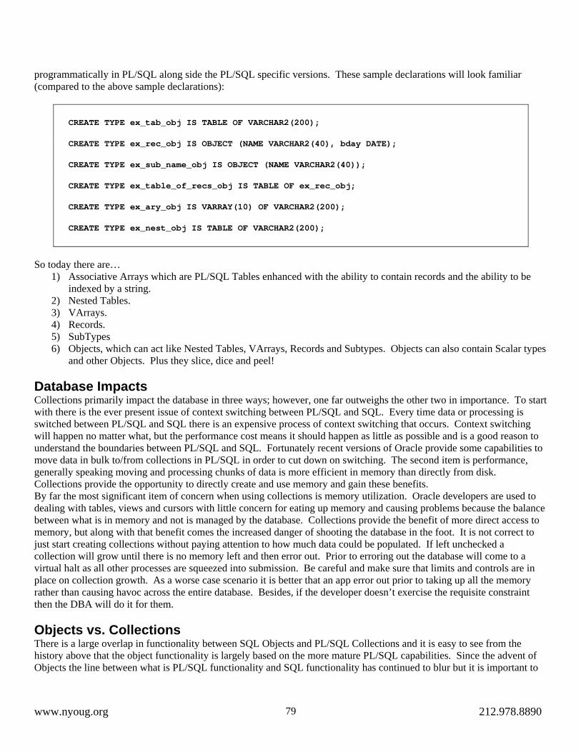
programmatically in PL/SQL along side the PL/SQL specific versions. These sample declarations will look familiar (compared to the above sample declarations):

CREATE TYPE ex_tab_obj IS TABLE OF VARCHAR2(200);

CREATE TYPE ex_rec_obj IS OBJECT (NAME VARCHAR2(40), bday DATE);

CREATE TYPE ex_sub_name_obj IS OBJECT (NAME VARCHAR2(40));

CREATE TYPE ex_table_of_recs_obj IS TABLE OF ex_rec_obj;

CREATE TYPE ex_ary_obj IS VARRAY(10) OF VARCHAR2(200);

CREATE TYPE ex_nest_obj IS TABLE OF VARCHAR2(200);

So today there are… 1) Associative Arrays which are PL/SQL Tables enhanced with the ability to contain records and the ability to be

indexed by a string. 2) Nested Tables. 3) VArrays. 4) Records. 5) SubTypes 6) Objects, which can act like Nested Tables, VArrays, Records and Subtypes. Objects can also contain Scalar types

and other Objects. Plus they slice, dice and peel!

Database Impacts Collections primarily impact the database in three ways; however, one far outweighs the other two in importance. To start with there is the ever present issue of context switching between PL/SQL and SQL. Every time data or processing is switched between PL/SQL and SQL there is an expensive process of context switching that occurs. Context switching will happen no matter what, but the performance cost means it should happen as little as possible and is a good reason to understand the boundaries between PL/SQL and SQL. Fortunately recent versions of Oracle provide some capabilities to move data in bulk to/from collections in PL/SQL in order to cut down on switching. The second item is performance, generally speaking moving and processing chunks of data is more efficient in memory than directly from disk. Collections provide the opportunity to directly create and use memory and gain these benefits. By far the most significant item of concern when using collections is memory utilization. Oracle developers are used to dealing with tables, views and cursors with little concern for eating up memory and causing problems because the balance between what is in memory and not is managed by the database. Collections provide the benefit of more direct access to memory, but along with that benefit comes the increased danger of shooting the database in the foot. It is not correct to just start creating collections without paying attention to how much data could be populated. If left unchecked a collection will grow until there is no memory left and then error out. Prior to erroring out the database will come to a virtual halt as all other processes are squeezed into submission. Be careful and make sure that limits and controls are in place on collection growth. As a worse case scenario it is better that an app error out prior to taking up all the memory rather than causing havoc across the entire database. Besides, if the developer doesn’t exercise the requisite constraint then the DBA will do it for them. Objects vs. Collections There is a large overlap in functionality between SQL Objects and PL/SQL Collections and it is easy to see from the history above that the object functionality is largely based on the more mature PL/SQL capabilities. Since the advent of Objects the line between what is PL/SQL functionality and SQL functionality has continued to blur but it is important to

www.nyoug.org 212.978.8890 79

understand that they are different, what the differences are and what it means for standard usage and managing complexity. Objects Do More Objects have instance methods, static methods, multiple constructors, comparison methods and persistence which is a lot of additional functionality and additional complexity. When you need all of this it is great, but when you don’t it is just overwhelming. Remember just because a feature exists doesn’t mean it has to be used. Objects Require More Memory The curse of having more functionality is the baggage it brings along, so simple objects are heavier (in almost every aspect) than similar PL/SQL constructs. Of course as the need for complexity increases the additional built in functionality may be worthwhile. Objects Are Fast But Slower Than Collections Relative performance and its cost/complexity is the focus of this document. A simple example below will show that when processing chunks of data, objects are significantly faster than traditional PL/SQL approaches but not as fast PL/SQL Collections and the related bulk operations. Objects Cannot Have or Be An Associative Array As stated before Associative Arrays can be very useful in some circumstances so if they are important to a specific application Objects aren’t an option. Objects Can Be Persisted As-Is Part of the problem with learning Objects in Oracle is all the information around how to store and retrieve them. It’s a heady topic and requires extra effort to understand and do correctly. What get’s little attention is that objects can be used nicely and relatively simply without being stored. Storing Objects is a good option and should be used where appropriate. PL/SQL constructs can be stored but there is no native support in the database and therefore must be “converted” into something different for persistence. Differences in Bulk Operations PL/SQL collections can be used in all bulk operations but Objects are only used in a “Select Into” bulk operation. There are other ways to have an Object Collection do mass updates and inserts which will be shown in one of the examples below. Objects Are Fullfledged Database Citizens It’s been said previously and if you have some experience with Oracle you have likely decided that I don’t know what I’m talking about. Everyone knows that Oracle fixed this in 10g so that any public type created in a PL/SQL package can be used like an Object. This is an important detail because there are performance and usage differences between the two so there are decisions to be made about which one should be used. Many developers have used PL/SQL collections for many years but haven’t done anything with Objects so they prefer to stick with what they know especially since it works for them. The reality is that Oracle didn’t “fix” anything instead they “faked” it so that any time a PL/SQL type is being used in a SQL manner it is really leveraging an Object. That’s right, Oracle makes an Object that is like the PL/SQL type and then does the translation for you…most of the time. Don’t believe it…take a look at the first example below.

www.nyoug.org 212.978.8890 80

No PL/SQL Types in SQL

This is a screen shot of the results from selecting all types from an empty schema. This would return all Objects (ie SQL types from the “CREATE OR REPLACE TYPE…” command). Since it’s an empty schema, there are no types.

This shows a package containing various public types being added to the empty schema.

www.nyoug.org 212.978.8890 81

Still no schema types…

Here is a new function being created which uses one of the PL/SQL types from the prior package.

www.nyoug.org 212.978.8890 82

Check the SQL Types again and we see something odd…new types that we didn’t create and they have crazy names.

Here is another new function which uses one of the PL/SQL types from the prior package.

www.nyoug.org 212.978.8890 83

Now there is another new SQL type with another crazy name. Maybe the declarations will tell us something:

CREATE OR REPLACE TYPE SYS_PLSQL_71957_DUMMY_1 AS TABLE OF NUMBER; CREATE OR REPLACE TYPE SYS_PLSQL_71957_9_1 AS TABLE OF NUMBER(1); CREATE OR REPLACE TYPE SYS_PLSQL_71957_24_1 AS TABLE OF DATE;

When the new functions were compiled Oracle added SQL Types behind the scenes to act as translations between SQL and PL/SQL. So if a PL/SQL Type is ever used in SQL, a SQL Object is involved whether intentionally or because Oracle handled it sight unseen. If that’s the case, why not just use the object to begin with? Close examination leads to another confusing detail. No SQL was ever involved, it was only PL/SQL (package and functions) so why was a SQL object created? The rules behind when one of these translation objects are created is not documented, but in this circumstance it is likely because the functions are pipelined, which is a significant indicator that the functions will be used in SQL. If Oracle provides a translation behind the scenes then they are as good as full fledged database citizens why worry about it? First, as discussed prior, there are differences in performance characteristics so it is best to know and control what is happening. Second, it increases complexity and overall messiness to have a bunch of “dummy” Objects lying around instead of having Objects created, named and used appropriately. Third, if there is ever a need to use some additional Object functionality it is not readily available. Fourth, even with this translation they are not full fledged citizens, they are wedged in and may not be usable in every circumstance. Here is an example of such a situation.

www.nyoug.org 212.978.8890 84

Here is a simple SQL Object with no methods other than the default constructor which is there but doesn’t need to be written by the developer.

Here is another Object that is a Nested Table of the prior Object. This object also has an unseen default constructor.

www.nyoug.org 212.978.8890 85

It is clearly possible that the object can be used from SQL. Please note that the IDE used for this example nicely separates the values into “columns” but that is not normal behavior and it will look different in SQL*Plus or SQLDeveloper. The function “tr_object” is exactly that, it is a call to the default constructor function for the object. This can be a good way to debug objects especially if they are more complex and have multiple constructors. If it is an individual object (not a collection) then it should be referenced in the SELECT portion of the statement.

www.nyoug.org 212.978.8890 86

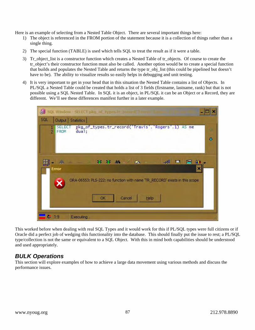
Here is an example of selecting from a Nested Table Object. There are several important things here: 1) The object is referenced in the FROM portion of the statement because it is a collection of things rather than a

single thing.

2) The special function (TABLE) is used which tells SQL to treat the result as if it were a table.

3) Tr_object_list is a constructor function which creates a Nested Table of tr_objects. Of course to create the tr_object’s their constructor function must also be called. Another option would be to create a special function that builds and populates the Nested Table and returns the type tr_obj_list (this could be pipelined but doesn’t have to be). The ability to visualize results so easily helps in debugging and unit testing.

4) It is very important to get in your head that in this situation the Nested Table contains a list of Objects. In PL/SQL a Nested Table could be created that holds a list of 3 fields (firstname, lastname, rank) but that is not possible using a SQL Nested Table. In SQL it is an object, in PL/SQL it can be an Object or a Record, they are different. We’ll see these differences manifest further in a later example.

This worked before when dealing with real SQL Types and it would work for this if PL/SQL types were full citizens or if Oracle did a perfect job of wedging this functionality into the database. This should finally put the issue to rest; a PL/SQL type/collection is not the same or equivalent to a SQL Object. With this in mind both capabilities should be understood and used appropriately. BULK Operations This section will explore examples of how to achieve a large data movement using various methods and discuss the performance issues.

www.nyoug.org 212.978.8890 87

This is the traditional loop method of moving 3,000,000 rows from one table to another. This took roughly 4 minutes on the test system and required very little memory.

This follows the standard of doing it in SQL which is possible for this simple example but not always possible. It ran in roughly 15 seconds and required very little data and took very little memory.

www.nyoug.org 212.978.8890 88

This is an example of using a PL/SQL collection (of records) with bulk collect and bulk insert (the FORALL construct was created for bulk DML operations). This code is small because Oracle doesn’t require the referencing of each column if the Record and Table structures match. SQL objects were not involved…hidden or otherwise. This ran in roughly 30 seconds and took approximately 1.2Gb of memory.

www.nyoug.org 212.978.8890 89

Procedure proc_big_data_obj shows the same data movement but it uses a SQL Object. The bulk collect could be used for the select statement, however since it uses a SQL Object it had to call the constructor; whereas, the PL/SQL collection example could do a “SELECT *…INTO…”. The reason this difference is necessary is mentioned above but deserves repeating, a SQL Object is an object and a PL/SQL collection/record is not…they are different and require different treatment. Bulk inserts are not allowed for Objects; however, the fact that they are SQL Objects allows a selection to be done directly on the collection. This ran in roughly 60 seconds and took approximately 1.4 Gb of memory. External Usage Oracle Objects are just that…Oracle Objects. They do not exist in the same form in other databases nor can they be instantiated inside some other object engine/software (ie .Net, Java, C++). There are ways to interact with Oracle Objects from other languages but they aren’t easy and one of the goals for controlling complexity is to make a simple to use API. This section will show how to apply what has been learned so far in ways that are easy and comfortable outside the database.

Assume for a moment that we want to pass a collection of SQL Objects as part of our API like the example above.

www.nyoug.org 212.978.8890 90

The above vb.net example shows that by using a select statement and the TABLE function the data is easily accessed as if it were a normal select statement.

www.nyoug.org 212.978.8890 91

The same goes for Java. It is important to note that older libraries may balk at the TABLE function but in this situation there are a couple other options:

1) Create a view which uses the TABLE function. The logic for not doing this in every situation is that a view must materialize every possible row before filtering but a direct select would allow the use of functions that take parameters that limit the rows returned potentially saving considerable resources.

2) Create a function that takes an IN OUT cursor as a parameter and the cursor is filled in the function but used in java/.net. This isn’t nearly as simple but is still more common knowledge for developers using data sources.

Controlling Complexity Now that there is a basic understanding of the options it is time to use the knowledge to create some guidelines to standardize (simplify) a majority of the code.

www.nyoug.org 212.978.8890 92

Apply 20%, 80% of the Time 1) If a type is never going to be used by SQL then use the PL/SQL functionality.

2) If there is a > 20% chance that a type will be used by SQL then use an Object.

3) Use a Nested Table in both SQL and PL/SQL. Allow others their 20%

1) Don’t store (persist) Objects.

2) API’s should both return Object Collections and fill an IN OUT Cursor.

3) Use the TABLE function.

4) Use other object capability like custom constructors when it will further simplify usage.

Objects should simplify and/or flatten the interface to complex data. This point has not been specifically discussed above but follows the principles of managing complexity. Object oriented design and development when done correctly have their advantages and it is possible to develop significant object oriented systems in Oracle but that should be a special and specific undertaking. This paper is focused on the more common relational data models and is more specifically focused on making things less complex so the recommendation is that Oracle Objects be used to simplify and if they don’t simplify then they probably shouldn’t be used.

SIGS, SIGS and more SIGS!

The following Special Interest Groups (SIG) hold meetings throughout the year for the benefit of NYOUG members:

DBA SIG – Database Administration

Data Warehouse SIG – Business Intelligence Web SIG – Web / XML / Java / 9iAS

Long Island SIG – Nassau/Suffolk area - All topics (Sponsored by Quest Software)

www.nyoug.org 212.978.8890 93

Forms Roadmap for Developers

Gilbert Standen, Sr. Consultant, TUSC, [email protected]

Managing Partner, Stillman Real Consulting LLC, [email protected] Oracle RDBMS Consulting for 12 years to private industry and governmen

INTRODUCTION This paper will give a roadmap of the various upgrade options of Forms software and the business justifications which would recommend and determine the necessity of such upgrades to Forms software. The paper will also discuss the toolsets which can be used to carry out continued Forms development and the considerations when choosing such tools. Finally the paper will discuss Forms in the context of Service Oriented Architecture (SOA) interoperability with other applications. Forms Software Upgrade Options Below are some important URL’s which will point you to the relevant upgrade documentation from Oracle for getting from the version of Forms being used in your enterprise to an upgraded version. The decision regarding whether or not you, as a developer, should support an upgrade recommendation to your organization is discussed in other sections of this paper. Bear in mind that Only Forms 6.0, Forms 6i, and Oracle9i Forms are supported for direct upgrade to Oracle Forms 10g (9.0.4) and then you can upgrade from there to the most recent versions of Forms. Older versions of Forms should be upgraded to Forms 6i or 9i first. Also bear in mind that applications that for whatever reason must run in Client Server or Character Mode should remain in Forms 6i and should not be upgraded. Some Important URLs for Forms Upgrade Planning Oracle URLs for Detailed Forms Roadmaps http://www.oracle.com/technology/products/forms/htdocs/upgrade/roadmap.html Oracle URLs for the Forms Upgrade Center http://www.oracle.com/technology/products/forms/htdocs/upgrade/index.html Oracle URL for Latest Statement of Direction (SOD) http://www.oracle.com/technology/products/forms/pdf/10g/ToolsSOD.pdf Oracle URL for Forms Roadmap Viewlet http://www.oracle.com/technology/sample_code/products/forms/viewlets/10g/forms_roadmap/Roadmap_viewlet_swf.html After reading these URL’s it should become apparent to you, if you don’t already know it, that Oracle Forms is one of the deepest product offerings in terms of number of organizations using older and wide-ranging legacy versions of an Oracle product, and that Oracle recognizes this. In other words, while we rarely see anymore Oracle 6 RDBMS out in the enterprises, we do see an amazing range of Forms products still being actively used in production applications, easily as far back as SQL*Forms 3.0 which continues to be used in a significant number of production applications. Because of this, Oracle Corporation, in the above URL’s, continues to provide a large base of documentation for helping shops migrate up from Forms as far back as SQL*Forms 3.0 as exemplified by the rich literature base in the URL links above. As a developer, you may become involved in making recommendations to your organization regarding whether or not an upgrade of the existing Oracle Forms environment(s) at your enterprise is worth doing. You may be asked to provide input on the technical aspects and the justifications for such an upgrade. The main reason to consider an upgrade to your existing Forms deployment is if there is a business need to do so within the context of your entire expected enterprise environment interoperability needs. We can break down these business

www.nyoug.org 212.978.8890 95

http://www.oracle.com/technology/products/forms/htdocs/upgrade/roadmap.html

http://www.oracle.com/technology/products/forms/htdocs/upgrade/index.html

http://www.oracle.com/technology/products/forms/pdf/10g/ToolsSOD.pdf

http://www.oracle.com/technology/sample_code/products/forms/viewlets/10g/forms_roadmap/Roadmap_viewlet_swf.html

http://www.oracle.com/technology/sample_code/products/forms/viewlets/10g/forms_roadmap/Roadmap_viewlet_swf.html

needs into 4 main criteria which can help to indicate if upgrading your Oracle Forms to a more fully SOA-compatible version of Forms is a decision which makes sense for your enterprise computing environment: 1. Will your forms need to interoperate with a J2EE based application? 2. Do you have business logic which changes often that would benefit from SOA? 3. Do you need to be on a fully-supported, latest-release version of Oracle Forms? 4. Is your organization moving to Windows Vista for Forms clients? If your Forms application is an isolated application which is unlikely to interoperate with any J2EE application then there may not be a good business justification to upgrade. The only justification in such a situation would be to keep current with fully supported Oracle products, which, in and of itself, does have some value to the organization, but may not be sufficient justification for your enterprise, at this time. Bear in mind that when we say fully-supported we mean patches, break-fixes, etc., which in many organization with static Forms deployments are unlikely to ever be needed. If your Forms application, on the other hand, is an application which now or in the future may be foreseen to require interoperation with other J2EE applications, it would be wise to migrate to at least Forms9i and from there plan to move up to keeping current with Forms releases, since maximum interoperability, and SOA-compability will be available in Forms 11 (not yet released) and in subsequent releases going forward as SOA compatibility for Forms is a major stated goal of Oracle Corporation1. Forms cannot yet (as of version 10.1.2) easily register an interest in a BPEL event and automatically be notified if input is needed from Forms. In version 11 of Forms, Oracle intends per their SOD to have functionality in place that will make this much easier (watch for updates on this from Oracle Corporation). Forms 11 also includes updates to the Java Importer tool which is PL/SQL wrappers for Java which is also a key element of integrating Forms into the SOA-BPEL landscape. Therefore it is suggested to set your sights on upgrading your Oracle Forms to Forms version 11. This version of Forms is currently slated to be the more fully “SOA-enabled” version of Forms, although any Forms version 9i or higher will position your enterprise to interoperate with J2EE. Key Forms Implementation Goals: • Forms which has Java Importer capability (PL/SQL wrappers for Java). • Forms which can register and get notifications from BPEL-compliant services • Forms 3-tier architecture deployment. Need to be on Forms 11 at a minimum • Timely application/awareness of SOA-BPEL-related Forms patches/upgrades If your Forms application is a stable, legacy application, with static unchanging business logic that is unlikely to ever be modified, again, you can choose not to upgrade. On the other hand, if your Forms application is likely to require new forms, and changes to business logic, then an upgrade to the most up-to-date release of Forms is in order, so that you may utilize tools such as the java importer, iPerspective, Vgo etc. to begin to decouple your business logic from your application by building services using SOA (service-oriented architecture). Also, you could consider using JDeveloper and Oracle ADF for engineering new application extensions, as well as making use of SOA where possible. If your Forms application needs to be running on software, for whatever reason, that is fully supported by Oracle, perhaps for legal or compliance reasons, then again, you should upgrade. Finally, if your organization plans a move to Windows Vista, there are technical issues related to using Jinitiator which would strongly recommend an upgrade at Forms 10g or conversely would recommend not upgrading to Windows Vista. This is because Jinitiator is known to be incompatible with Windows Vista. With regard to the issues with Jinit vs. Sun generic JVM, when upgrading to the upcoming Forms 11 for example, you would push J2EE version 6 to your client community machines (Sun JRE 1.6.x_x) at that point, and at which time Jinitiator would be decommissioned and can (optionally) be deinstalled from clients. It is this author’s position, however, that enterprise upgrades to Windows Vista should not be drivers of Oracle Forms upgrade decisions.

1 Oracle Forms-Oracle Reports-Oracle Designer: Statement of Direction An Oracle White Paper October 2008 at http://www.oracle.com/technology/products/forms/pdf/10g/ToolsSOD.pdf

www.nyoug.org 212.978.8890 96

http://www.oracle.com/technology/products/forms/pdf/10g/ToolsSOD.pdf

The widely-discussed incompatibility of Jinitiator with Windows Vista can be considered a peripheral “smoke” issue and is not a primary driver for a Forms upgrade, unless your organization is firmly committed to a Windows Vista enterprise upgrade in which case you must make the cutover from Jinit to Sun JRE. Other Reasons Include2 3 4: 1. Oracle has no plans to certify Jinit with Oracle E-business version 12; 2. Eliminate JVM vs. Jinit client workstation conflicts; 3. Deploy a single JVM to client workstations. All of the above are encompassed in Forms 11 and so this is a logical point at which to make the upgrade to Forms 11, the cutover to Sun JRE, and the decommissioning of Jinitiator. SUGGESTED UPGRADE STRATEGIES This suggests that a possible strategy would be to start planning ahead now to do one sweeping, major upgrade event when Forms 11 is released: Proposed “Leveraged Strategy” Upgrade Plan Steps 1. Upgrade Forms to version 11 2. Upgrade Database(s) to 11g 3. Recompile all Forms applications (RSF-Pl/Sql) 4. Reconfigure Forms to push Sun JRE 6 to clients 5. Decommission and Uninstall Jinitiator from clients 6. Optionally can now upgrade clients to Win Vista. Rationale and Justification for Upgrade Strategy • Positions existing Forms as SOA-BPEL compatible, enabled and “compliant”. • Positions existing Forms to be using J2EE version 6 of the client JRE (JRE 1.6.x_x) which is the generic Sun JRE

version certified for Forms 11. • Implements the REQUIRED Jinitiator retirement. • Requires your organization to only deal ONCE with the re-compiling of all Forms applications due to the Database

RSF – PL/SQL compatibility requirement across major database releases (e.g. 10g -11g)5 • Leverages new Oracle 11g RDBMS features. • Positions you to be able to go to Windows Vista on clients (optional). However, if you are on early versions of Forms, how do you get this upgrade accomplished? Roadmaps for the upgrade paths can be found at this URL: http://www.oracle.com/technology/products/forms/htdocs/upgrade/roadmap.html 2 Oracle Forms 10g Release 2 (10.1.2.x) Statement of Directions (May 22, 2008) http://www.oracle.com/technology/products/forms/htdocs/10gR2/clientsod_forms10gR2.html 3 Oracle Forms in the SOA World by Robin Zimmermann http://www.oracle.com/technology/oramag/oracle/05-mar/o25forms.html 4 Oracle Forms & a Service Oriented Architecture (SOA): A Whitepaper from Oracle Inc. June 2007 http://www.oracle.com/technology/products/forms/pdf/10gR2/forms-soa-wp.pdf 5 Smoother version-to-version upgrade commitment from Oracle should make this easier.“Oracle will allow compatibility changes between Database Required Support Files (RSF’s) and PL/SQL versions to occur ONLY across major releases of the database”

www.nyoug.org 212.978.8890 97

http://www.oracle.com/technology/products/forms/htdocs/upgrade/roadmap.html

http://www.oracle.com/technology/products/forms/htdocs/10gR2/clientsod_forms10gR2.html

http://www.oracle.com/technology/products/forms/htdocs/10gR2/clientsod_forms10gR2.html

http://www.oracle.com/technology/oramag/oracle/05-mar/o25forms.html

http://www.oracle.com/technology/products/forms/pdf/10gR2/forms-soa-wp.pdf

http://www.oracle.com/technology/products/forms/pdf/10gR2/forms-soa-wp.pdf

This roadmap will take you from as far back as Forms character mode and give you an upgrade Roadmap to bring you as far up the Forms chain of upgrades as you want to go, up to and including Forms 11 (when released). Forms 6i Forms 9i Upgrade Considerations If you are going from Forms 6i to Forms 9i you should review this URL: http://www.oracle.com/technology/products/forms/pdf/forms_upgrade_reference.pdf It contains detailed information about what sorts of Forms functionality will be lost when you make this upgrade, and what you can expect in terms of the effect on your existing Forms 6i application. The most desirable strategy would be to have a test environment which is refereshed up to date and can be upgraded to test out the upgrade and then put through a rigorous well-planned User Acceptance Testing (UAT) phase prior to carrying out the actual production upgrade. Environment Modeling Any Oracle Forms upgrade being considered for a mission-critical application should be modeled and tested carefully before carrying out the actual upgrade. REFERENCES Moving from Oracle Forms to Java the easy way http://www.in2j.com/docs/in2j_whitepaper_291008.pdf

www.nyoug.org 212.978.8890 98

http://www.oracle.com/technology/products/forms/pdf/forms_upgrade_reference.pdf

http://www.in2j.com/docs/in2j_whitepaper_291008.pdf

NYOUG 2009 Sponsors

The New York Oracle Users Group wishes to thank the following companies for their generous support.

Confio Software (www.confio.com)

GoldenGate Software (www.goldengate.com) IBM (www.ibm.com)

Oracle (www.oracle.com) Quest Software (www.quest.com)

TUSC (www.tusc.com)

Contact Sean Hull and Irina Cotler for vendor information, sponsorship, and benefits

www.nyoug.org 212.978.8890 99

What’s waiting for you at Oracle OpenWorld 2009? Over 42,000 Oracle® clients are expected to attend Oracle OpenWorld, the world's largest event dedicated to helping enterprises understand and harness the power of information. Convening in San Francisco, from October 11 to 15, 2009, this event will showcase the customers and partners whose innovation with Oracle translates to better business results — for their companies, and quite possibly for yours as well.

As one of the top sponsors of Oracle OpenWorld 2009, IBM will offer sessions that demonstrate proven end-to-end solutions and capabilities around Oracle applications and technology. IBM and Oracle have worked together to solve complex business problems for clients for 20 years. Today, we are helping over 15,000 organizations of all sizes change the way they do business.

Learn more about IBM’s Data Management Solutions The IBM® Optim™ team will be participating at Oracle OpenWorld, along with members of the IBM's Global Services, Hardware, Cognos, Data Mirror and other brands. In addition, IBM and the Optim team will be hosting several special events which you won't want to miss.

You and your colleagues are encouraged to take advantage of this event to obtain all the technology information you need and have all your questions answered — in one convenient location.

Visit IBM at Booth #733, Moscone Center South Learn about IBM's innovative industry solutions, business process and technology solutions, as well as information management solutions. Live demonstrations and “Ask the Experts” sessions will be scheduled throughout the conference.

IBM Optim has been widely accepted as the leading data management solution for users of Oracle products and has been featured at this conference for many years. Optim provides proven enterprise data management capabilities across Oracle’s leading ERP and CRM applications in use today – Oracle® E-Business Suite, PeopleSoft® Enterprise, JD Edwards® EnterpriseOne and Siebel® CRM, as well as your custom and packaged applications that run on Oracle databases. Optim will be featured in many sessions, so please stop by and learn about the latest features and enhancements.

Attend IBM Optim Speaking Events Plan to attend many of the IBM Optim speaking events to learn how you can address enterprise data critical business issues, such as data growth management, data privacy compliance, test data management, e-discovery, application upgrades, migrations and retirements. Take advantage of the opportunity to attend sessions on how you can improve enterprise data management and derive more value from your investment in Oracle ERP and CRM applications.

Developing Web Applications with XML and Oracle - Nyoug

Documents

Transcript of Developing Web Applications with XML and Oracle - Nyoug