Developing and testing poverty assessment tools: Results ... Accuracy Report.pdf · Developing and...
81
microREPORT Developing and testing poverty assessment tools: Results from accuracy tests in Bangladesh Manfred Zeller Gabriela Alcaraz V. Julia Johannsen November 2004 Accelerated Microenterprise Advancement Project
Transcript of Developing and testing poverty assessment tools: Results ... Accuracy Report.pdf · Developing and...
mic
ro
RE
PO
RT
Developing and testing poverty assessment tools:Results from accuracy tests in Bangladesh
Manfred Zeller
Gabriela Alcaraz V. Julia Johannsen
November 2004
Accelerated Microenterprise Advancement Project

Accelerated Microenterprise Advancement Project (AMAP) is a 4-year contracting facility that USAID/Washington and Missions can use to acquire technical services to design, implement, or evaluate microenterprise development, which is an important tool for economic growth and poverty alleviation. For more information on AMAP and related publications, please visit www.microLINKS.org. Contract Number: GEG-I-02-02-00029-00 Task Order No. 2: Developing Poverty Assessment Tools Contractor: The IRIS Center at the University of Maryland Manfred Zeller, Ph.D., is full professor for Socioeconomics of Rural Development at the University of Göttingen, Germany. Gabriela Alcaraz V. and Julia Johannsen are Ph.D. candidates of the Institute of Rural Development, University of Göttingen, Germany. The IRIS Center is a research and technical assistance provider housed at the University of Maryland, College Park.
Contents
Introduction ....................................................................................................................................................1 1.1 Field survey for accuracy tests in Bangladesh .....................................................................2 1.2 Sampling Frame ...................................................................................................................2 1.3 Poverty line...........................................................................................................................3 Overview of Regression Analysis ..................................................................................................................6 2.1 Introduction ..........................................................................................................................6 2.2 Composite Questionnaire .....................................................................................................6 2.3 Selection of indicators ..........................................................................................................7 2.4 Specification of regression models.......................................................................................9 2.5 Differences between the models.........................................................................................10 Results from Regression Models..................................................................................................................15 3.1 Model 1...............................................................................................................................16 3.2 Model 2...............................................................................................................................18 3.3 Model 3...............................................................................................................................19 3.4 Model 4...............................................................................................................................20 3.5 Model 5...............................................................................................................................22 3.6 Model 6...............................................................................................................................23 3.7 Model 7...............................................................................................................................25 3.8 Model 8...............................................................................................................................26 3.9 Model 9...............................................................................................................................27 Practitioner Tools .........................................................................................................................................29 4.1 Loan size tool .....................................................................................................................29 4.2 Accuracy tests of Participatory Wealth Ranking ...............................................................31 4.3 Poverty incidence among clients of financial institutions..................................................45 Summary ......................................................................................................................................................47 5.1 Brief synthesis of results ....................................................................................................47 5.2 The issue of unbalanced accuracies....................................................................................48 5.3 Practicality issues ...............................................................................................................51 Bibliography.................................................................................................................................................52 Annexes ........................................................................................................................................................53 Annex A: Size and distribution of sample....................................................................................53 Annex B: Descriptives of all regressors (n= 253), by type of model...........................................54 Annex C: Gender-specific variables used in regression analysis..................................................66 Annex D: Verifiability scores provided by survey firm DATA in Bangladesh...........................67 Annex E: Summary table of the results........................................................................................72 Annex F: Variables included as 15 best regressors, by model ......................................................73 Endnotes .......................................................................................................................................................76


Introduction 1
Introduction
USAID has commissioned the IRIS Center to develop, test and disseminate poverty assessment tools which will meet Congressional requirements for accuracy and cost of implementation. Accuracy tests of poverty indicators have been implemented by IRIS in Bangladesh, Peru, Uganda, and Kazakhstan. Comprehensive information on the project is available at www.povertytools.org, and will not be summarized in this report.
The purpose of this report is to present the results of the accuracy tests in Bangladesh1. In the remaining part of chapter 1, we provide an overview of the design of the field research for the accuracy test, and the computation of the applicable poverty line. Chapter 2 provides an overview of the analysis presented in this report.
In chapter 3, we present the results on selected poverty indicators from 9 regression models. Each of these models can be viewed as a potential, newly designed poverty assessment tool which is calibrated for Bangladesh based on a nationally representative sample. The regression models are run in SAS, using the function MAXR that seeks to maximize the explained variance of the dependent variable (per-capita daily expenditure) by a set of best 5, best 10, and best 15 regressors. Any set of five, ten, or fifteen poverty indicators can be considered a poverty assessment tool for purposes of identifying the poverty status of a household. The first 6 regression models differ with respect to the set of poverty indicators allowed in the model, starting from a model with a full set of potential regressors, and gradually restricting the set of regressors on the basis of practicality in implementation. A seventh model is run as an example of a tool that considers only those poverty indicators that were rated as highly verifiable by DATA, the survey firm in Bangladesh. A subsequent model compiles these indicators with powerful subjective as well as monetary indicators. Finally, the last model makes use of poverty indicators usually available in Living Standards Measurement (LSMS) surveys. Thus, the first eight models can be considered alternative best combinations of poverty indicators which were mainly derived from existing practitioner tools for poverty assessment, while model 9 is a tool derived from poverty indicators usually available in LSMS surveys.
Chapter 4 goes on to address two other methods of poverty assessment. The first section assesses the accuracy of loan size as a predictor of poverty status, a method that has been widely used by the micro-finance industry so far. The second section assesses the accuracy of participatory wealth ranking. Chapter 5 summarizes the results.

2 Developing Poverty Assessment Tools Accelerated Microenterprise Advancement Project
1.1 Field survey for accuracy tests in Bangladesh
The survey firm Data Analysis and Technical Assistance (DATA)2 in Dhaka, Bangladesh carried out the survey and completed double entry of data using SPSS Data Entry software. In total, 30 interviewers in five teams implemented the composite questionnaire survey with 800 households, followed two weeks later by the benchmark questionnaire. Training of the interviewers began on February 17, 2004. The survey was carried out from March 17 to April 15, and double entry of all data was completed by July 15, 2004.
The questionnaires can be downloaded at www.povertytools.org. The composite as well as the benchmark questionnaire required adaptation to the country-specific context. In the case of the composite questionnaire, this entailed the inclusion of country-specific poverty indicators, such as the number of saris owned, or the inclusion of certain inferior foods in Section E (see questions E151 thru 157). Useful sources for the identification of country-specific poverty indicators include: a number of official statistical reports (BBS, 2002; and BBS, 2003); results from the FANTA Food Insecurity and Vulnerability Project implemented by Dr. Patrick Webb (formerly with Tufts University, now with World Food Program); and a publication by Matin et al. (2003) concerning the adaptation and use of the CGAP Poverty Assessment Tool (Henry et al. 2003; Zeller et al. 2001) in Bangladesh. The adaptation of the benchmark questionnaire mainly involved the selection of major food items. For this we referred to results from the most recent Household Income and Expenditure Survey (HIES, 2000), as well as a report published by the International Food Policy Research Institute (Zeller et al, 2002.)
The adaptation of the two questionnaires has benefited greatly from the long-term expertise of the personnel of DATA, its managing director Md. Zahidul Hassan and director Md. Zobair, as well as their supervisors and interviewers, in conducting poverty, food security, and expenditure surveys during the past 15 years in Bangladesh.
Two employees of DATA with considerable experience in qualitative as well as quantitative research methods participated in a three-day training session on Participatory Wealth Ranking held at the Bangladesh Academy for Rural Development in Comilla. This training session was led by Dr. D.S.K Rao, and organized by PKSF in the scope of the Asia-Pacific Region Microcredit Summit Meeting of Councils in February of 2002.
1.2 Sampling Frame Requirements for sampling. In view of budget and time constraints, it was determined to choose a sample size of 800 households. The sample was required to be nationally representative.
The highest administrative unit in Bangladesh are so-called divisions. The six divisions are further disaggregated into a total of 64 districts. Each district has on average about 8 counties (so-called Thanas). There are about 500 Thanas in the country. Each Thana holds a number of

Introduction 3
unions. A union consists of several villages or urban wards. Within those, one can distinguish hamlets (Para) at the local level.
A multi-stage cluster sampling approach was used in drawing up a random sample of households. This sampling procedure allows us to draw successive samples at lower administrative units, a feature that was useful in Bangladesh since data on size of population are published only for the division, district and Thana level. In order to minimize sampling error, the first stage of sampling was at the Thana level, as the lowest administrative level with centrally available and published population data. In view of logistical and budget constraints, it was determined to randomly select 10 Thanas out of the total of Thanas. The randomly selected Thanas are located in five of the six divisions of Bangladesh (excluding Sylhet division: See annex A).
The probability of selecting a certain Thana was equal to its share of population in the country. This so-called probability-proportionate-to-size sampling (PPS) was repeated at the second stage. Here, out of the total of unions in each of the ten selected Thanas, two unions were randomly chosen proportionate to size of the unions compared to total population size in the Thana. In each of the twenty unions, one village was then randomly selected, again with a probability proportionate to size of village within a given union. (Because the union and village data of the population census 2001 was not yet published in February 2004, the latest population data on unions and villages could only be obtained at the administrative headquarters of the Union or the Thana.)
Finally, in each of the 20 randomly selected villages, the random walk method (see Henry et al. 2003) was applied to select a random sample of 40 survey households. Thus, the total sample size is 800, and the sample is a self-weighing, nationally representative sample. The sample for Participatory Wealth Ranking comprises a subsample of 320 (out of the 800) households located in 8 unions over 3 of the 5 divisions. This subsample has not been randomly selected. Because of logistical and budget constraints, a purposeful sample was chosen which sought to come up with the best possible set of districts considering criteria such as regional diversity, costs of transport and survey personnel, as well as timetable of overall survey operations.
1.3 Poverty line The legal text by U.S. Congress refers to two alternative poverty lines in defining the “very poor.” The term “very poor” refers to individuals
(A) living in the bottom 50% below the poverty line established by the national government; or
(B) living on the equivalent of less than $1/day. Through the above term “or”, the legislation implies that a person could be considered very poor if he/she was either living on less than a dollar a day, or was in the bottom half of the distribution
4 Developing Poverty Assessment Tools Accelerated Microenterprise Advancement Project
of those below the national poverty line. The legislation thus identifies two alternative measures of extreme poverty, relating to two commonly used poverty lines:
National Poverty Line (A): the bottom 50 percent of those classified as poor by any national poverty line. In Bangladesh, the national poverty line is expressed in Taka, the local currency. International Poverty Line (B): one dollar income per day per capita (equal to $1.08 per day in purchasing power parity (PPP) dollars at 1993 prices).
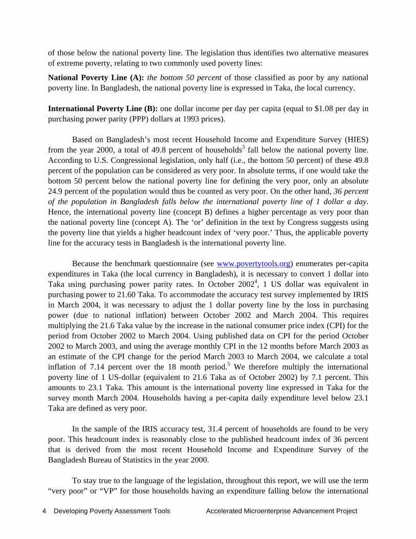
Based on Bangladesh’s most recent Household Income and Expenditure Survey (HIES) from the year 2000, a total of 49.8 percent of households3 fall below the national poverty line. According to U.S. Congressional legislation, only half (i.e., the bottom 50 percent) of these 49.8 percent of the population can be considered as very poor. In absolute terms, if one would take the bottom 50 percent below the national poverty line for defining the very poor, only an absolute 24.9 percent of the population would thus be counted as very poor. On the other hand, 36 percent of the population in Bangladesh falls below the international poverty line of 1 dollar a day. Hence, the international poverty line (concept B) defines a higher percentage as very poor than the national poverty line (concept A). The ‘or’ definition in the text by Congress suggests using the poverty line that yields a higher headcount index of ‘very poor.’ Thus, the applicable poverty line for the accuracy tests in Bangladesh is the international poverty line.
Because the benchmark questionnaire (see www.povertytools.org) enumerates per-capita expenditures in Taka (the local currency in Bangladesh), it is necessary to convert 1 dollar into Taka using purchasing power parity rates. In October 20024, 1 US dollar was equivalent in purchasing power to 21.60 Taka. To accommodate the accuracy test survey implemented by IRIS in March 2004, it was necessary to adjust the 1 dollar poverty line by the loss in purchasing power (due to national inflation) between October 2002 and March 2004. This requires multiplying the 21.6 Taka value by the increase in the national consumer price index (CPI) for the period from October 2002 to March 2004. Using published data on CPI for the period October 2002 to March 2003, and using the average monthly CPI in the 12 months before March 2003 as an estimate of the CPI change for the period March 2003 to March 2004, we calculate a total inflation of 7.14 percent over the 18 month period.5 We therefore multiply the international poverty line of 1 US-dollar (equivalent to 21.6 Taka as of October 2002) by 7.1 percent. This amounts to 23.1 Taka. This amount is the international poverty line expressed in Taka for the survey month March 2004. Households having a per-capita daily expenditure level below 23.1 Taka are defined as very poor.
In the sample of the IRIS accuracy test, 31.4 percent of households are found to be very poor. This headcount index is reasonably close to the published headcount index of 36 percent that is derived from the most recent Household Income and Expenditure Survey of the Bangladesh Bureau of Statistics in the year 2000.
To stay true to the language of the legislation, throughout this report, we will use the term “very poor” or “VP” for those households having an expenditure falling below the international
Introduction 5
poverty line of 1 dollar a day per person equivalent to 23.1 Taka, and the term “not very poor” or “NVP” for those having an expenditure equal or above the international poverty line. Readers should bear in mind that ANY such binomial, either/or labels tend to distort the underlying reality, which is continuous: the standard of living of a household just above the line is not that much different than that of a household just below the line. Thus, the term “not very poor” is simply shorthand for "estimated to have per capita daily consumption expenditures more than $1.08 a day at 1993 purchasing power parity.” We wish to note that a considerable share of these so-called not very poor are actually categorized as being poor by the national poverty line, and that even among those above the national poverty line there exist a considerable share of households that are vulnerable to poverty such that for example a bad harvest, an illness of a family member, or a social obligation may drive them into poverty.

6 Developing Poverty Assessment Tools Accelerated Microenterprise Advancement Project
Overview of Regression Analysis
2.1 Introduction
In Chapter 3, we analyze the accuracy of newly designed tools and develop nine regression models for generating tools. These models consider all the poverty indicators that were compiled in the composite questionnaire, based on submissions of practitioner tools to IRIS in late 2003 that are reviewed by Zeller (2003) (see www.povertytools.org). In addition, indicators have been included based on recent poverty assessment studies published in academic literature. Thus, with the exception of model 9 that uses LSMS type indicators only, the newly designed tools considered in chapter 3 seek best combinations from poverty indicators of existing practitioners tools.
2.2 Composite Questionnaire The structure of the composite questionnaire is as follows (see www.povertytools.org): A. Identification of household (location, client status etc.) B. Household roster/demography, including individual as well as household-level indicators
(derived from all practitioner tools) C. Household expenditures by category (adapted from FINCA and ACCION tool) D. Housing indicators (generic questions adapted from tools by AIM, ASA, CASHPOR,
CIMS-OI, PRIZMA, and TUP), plus poverty indicators concerning minimum wages acceptable to respondents
E. Food consumption/Food Security Scales (adapted from tools by CGAP, Freedom from Hunger, and World Food Program Food Security and Hunger Questionnaire)
F. Asset based indicators (adapted from GRAMEEN Network and most other tools) G. Social capital, voice and vulnerability (adapted from recent advancements in social science
research) H. Estimates of objective and subjective poverty (adapted from recent advancements in social
science research) I. Information on client status of individual household members in programs and institutions
supporting micro-finance or business development services (including information on size of loans and outstanding debt)
K. Monetary voluntary savings by individual household members (WOCCU)

Overview of regression analysis 7
2.3 Selection of indicators
In chapter 3, we present results from nine models that were run with ordinary least squares using the software SAS. The models differ by the type of regressors used. While Model 1 includes 253 regressors, the seventh model has the most restrictive list of 97 potential poverty indicators.
As one can see from the results for Model 1 in Chapter 3, the set of best6 poverty indicators is dominated by different expenditure and asset categories, apart from household demographic characteristics. In Model 1, there are only a few poverty indicators from other dimensions and sections of the composite questionnaire. In a gradual process starting with Model 2, we reduce the number of regressors so as to allow indicators from other dimensions and sections of the questionnaire to enter among the best set of poverty indicators. The overriding principle is to narrow down the list of poverty indicators with respect to two criteria:
Difficulty of indicators. Information on some indicators is easy to obtain, while for others it is not. Difficulty can be expressed in terms of time, money, and social costs expended for obtaining information. Social costs are especially important when addressing culturally sensitive questions. The difficulty of an indicator will therefore vary with the socio-economic and cultural context. It will also depend on the skill level and quality of training of interviewers. Furthermore, difficulty is strongly affected by the educational level and intellectual skills of the respondent, and by the interview situation (whether in private at home, or among peers and/or strangers in public—where certain type of questions may incur high social costs for the respondent). For example, the value of total assets is very difficult and tedious to obtain, and therefore is not really suitable for an operational poverty assessment tool. Another example is question C2 in the composite questionnaire, the value of food that is home-produced and consumed by the household in an average week, and several other expenditure indicators.
Verifiability of indicator. Another useful characteristic of an indicator for its operational use is its ease of verification (in terms of time, monetary and social costs). Here, we distinguish between objective and subjective indicators. Subjective indicators include any self-assessment (perception, feeling, attitudes) by the respondents (e.g., Section E9 onwards and Section H, regarding perceived adequacy of livelihood); or any assessment done by the interviewer (e.g., rating the poverty status of a household on a scale from 1 to 5, as in Section A). While some subjective indicators are among the more powerful poverty indicators, as will be shown later, they are hardly verifiable, as the scales used are subjective and not disclosed to others. Objective indicators are characterized by using scales for measurement that can be – at least in principle – verified by consistent standards of measurement metrics. Examples of objective indicators include the age of a person (in years), the size of the rooms (in square meters), or whether the roof is of natural fibers; these are directly measurable through conventional and universally comparable scales. Measurability using comparable scales is a prerequisite for direct verifiability.
8 Developing Poverty Assessment Tools Accelerated Microenterprise Advancement Project
Objective indicators, however, may also vary in their degree of verifiability. An example of an objective but hardly verifiable indicator is the number of luxury food eaten in the past 7 days, or the money received from migrant relatives, or how many days a child was sick in the past 12 months. Common to this group of hardly verifiable objective indicators is the fact that actions or states occurred in the past.
Having recognized in the above that the difficulty and verifiability of an indicator cannot be generalized across different socio-economic and cultural contexts, we acknowledge that it might appear rather arbitrary to classify a particular indicator (or a group of indicators) as being more or less difficult to ask, or more or less verifiable. Therefore, we understand that our selection of progressively smaller subsets of regressors for defining Model 1 thru Model 6 would be agreeable to any – and certainly not to all - readers. This approach mainly aims to develop a variety of tools that differ in the dimensions of poverty that are considered. Moreover, this approach should be understood as a first attempt to address the practicality issue by presenting different models with perhaps increasingly simple and verifiable indicators. In Model 7 and 8, we use the subjective assessment of verifiability of the survey firm DATA as an alternative attempt to address the practicality issue. To get more information on the practicality of poverty indicators, the IRIS project includes practicality tests carried out by microfinance (MF) and business development services (BDS) organizations.
Our sequence of regression models with progressively fewer poverty indicators (from Model 1 to Model 6) aims to generate different poverty assessment tools that gradually become less accurate but hopefully also more practicable, less costly, and less prone to falsification by respondents or survey intermediaries.
For each model presented in chapter 3, we present a set of BEST 5, BEST10, and BEST15 poverty indicators. Each of these three sets can be considered a poverty assessment tool in itself, and we document for each tool its level of overall accuracy, accuracy among the very poor and the not very poor, as well as the degree of undercoverage and leakage. From an operational point of view — and everything else being the same— a tool derived only from the five best indicators presents an easier, more practical poverty assessment tool than one that uses the best 15 (or even more) poverty indicators7. This is quite obvious: fewer questions are necessary to ask and to analyze with a BEST5 tool compared to a BEST15 tool. However, fewer poverty indicators in the tool usually also tend to imply a lower degree of accuracy.
This highlights the important trade-off between accuracy and practicality of a poverty assessment tool. Cutting the right balance here requires us to carefully consider the trade-offs between accuracy (and residual errors) and practicality, and this will ultimately determine the choice and certification of certain poverty assessment tools.

Overview of regression analysis 9
2.4 Specification of regression models
The following nine model types were run as ordinary least squares in SAS. In all regressions, the sample size is 799 (as one household has a missing benchmark interview). The dependent variable is the natural logarithm of per-capita daily expenditures in Taka, the national currency in Bangladesh.
Table 2.2.1 Dependent variable per capita daily expenditures
Variable N Minimum Maximum Mean Standard deviation
Per capita daily expenditures 799 7.45 151.44 35.96 22.35
Ln expenditures per capita (natural logarithm) 799 2.01 5.02 3.43 0.53
In all regressions, an INCLUDE statement always includes the following 7 regressors as
control variables: Table 2.2.2 Description of the seven control variables
Variable N Minimum Maximum Mean Standard deviation
Household size 799 1 24 4.93 2.10 Household size squared 799 1.00 576.00 28.75 32.34 Age of household head 799 18.00 85.00 44.64 13.46 Division 1 799 0 1 0.30 0.46 Division 2 799 0 1 0.20 0.40 Division 3 799 0 1 0.10 0.30 Division 4 799 0 1 0.30 0.44
The first three control variables take into account the influence of important demographic
factors that – in previous research - have been found powerful variables in explaining per-capita expenditures at the household level. As pointed out above, a division is the highest administrative unit within Bangladesh. The four dummy variables Division 1 thru 4 seek to capture regional differences. The inclusion of these four dummy variables ensures that the estimated regression coefficients are controlled by regional differences.
All variables that are defined in monetary values (such as for expenditures and assets) are converted into natural logarithms8 since the dependent variable is also expressed in natural logarithm. All ordinal variables (for example type of roof, with lower values indicating inferior materials and higher values indicating superior materials, or subjective rankings, such as the food security scales) have been converted into dummy variables that reflect the different subtypes. For example, if the database has three types of roof (1=natural material, 2=metal, 3=superior, such as

10 Developing Poverty Assessment Tools Accelerated Microenterprise Advancement Project
tile), then dummy variables for two of the three different types of roof were formulated and tested in the statistical analysis for their potential of being a significant poverty indicator.
The nine different models were run in SAS using the MAXR technique that seeks to obtain a model with a high R-square. The R-square (R2) is the ratio of the variance in the dependent variable that is explained by the model and its regressors, divided by the overall observed variance of the dependent variable. The coefficient ranges between 0 and 1. R2 takes on the value of 1 when predicted values for the dependent variable for all households are the same as the observed values. A coefficient of 0.6 for R2 implies that 60 percent of the observed variance in the dependent variable is explained by the model and its regressors.
High explanatory power of a model is a prerequisite for good predictions of the dependent variable per-capita daily expenditures (and thereby poverty status). The maximum R2
improvement technique (MAXR) is a subcommand for regressions in SAS. The MAXR technique seeks to maximize explained variance (i.e., R2), and considers all combinations among pairs of regressors to move from one step to the next. In the first step, the MAXR method begins by finding the one-variable model producing the highest R2. In the second step, another variable, the one that yields the greatest increase in R2, is added. Once the two-variable model is obtained, each of the variables in the model is compared to each of the variables not in the model. For each comparison of single pairs of variables, MAXR demonstrates whether removing one variable and replacing it with the other one increases R2. After comparing all possible switches, MAXR makes the switch that produces the largest increase in R2 . Comparisons then begin again in the third step and so forth, and the process continues until MAXR finds that no switch can increase R2. This limit may not be reached at 15 variables, but may include many more regressors. Thus, the MAXR technique allows us to identify the best model in each category: with only one, only 5 (termed in this paper the BEST5 model), only 10 (BEST10 model), only 15 (BEST15) model, or the best model using N regressors. The number N is determined by MAXR itself.
2.5 Differences between the models
From the composite questionnaire, we computed approximately 700 poverty indicators. Prior to using SAS software with the function MAXR, SPSS was used to analyze for each variable its potential as regressor. Basically, correlation as well as regression analysis was used to select potential regressors for SAS MAXR routine. By analyzing separately each of the poverty dimensions (i.e., the different sections of the composite questionnaire such as food security, agricultural assets, membership in organizations), correlation of indicator variables with the per-capita benchmark variable as well as step-wise regression models were used to select powerful regressors from each dimension. This procedure ensured that all of the dimensions of poverty (as well as all submitted poverty indicators from practitioner tools) were considered in the final regression analysis using SAS software, and hence in the generation of tools. Special care was given to the generation and testing of gender-specific poverty indicators. Annex C separately lists

Overview of regression analysis 11
the gender-specific indicators that were selected for the final regression analysis (i.e., subset of 253 regressors). The difference between the models are described next (see also Figure 2.5.1).
Model 1: This model includes all 253 regressors considered in the regression analysis using SAS software. As will be shown later, this model contains many regressors that are derived from indicators on expenditures or value of assets.
Model 2: In this model, we drop all expenditure related variables, except clothing expenditures per capita in past 12 month (see section B of the composite questionnaire). This variable was the single best expenditure category among 13 tested using SAS MAXR technique9. The variable clothing expenditure is also one of the easier ones to recall among the expenditure group. A reduction of the number of expenditure variables is a first step towards a more operational set poverty indicators. As pointed out, self-reported expenditures by respondent — irrespective of whether the recall period for expenditures is one week, one month or one year— are impossible to verify directly.
Moreover, the questions contained in section C (question C1 to C12) require relatively intensive interviewer training as they are prone to high measurement error in practice. The interviewer needs to facilitate the interview by asking prompting questions on major elements of the different expenditure categories. For example, a particularly difficult expenditure category is home-produced food—especially for interviewers unfamiliar with traditional (or metric) measures used for crop yields in agriculture and food subsistence production (see question C2). Furthermore, the interviewer needs to provide special assistance to respondents with no or low school education for even simple calculations such as adding up expenses, especially since some elements of a certain expenditure category are recalled by the respondent on a monthly basis, and others are best remembered on a weekly basis (1 bag of potatoes per month, but a basket of rice per week). While these questions did not pose any significant difficulties for the experienced interviewers of DATA (the survey firm in Bangladesh), they may pose difficulties for less experienced interviewers. In total, Model 2 has 235 regressors that were retained from Model 1 (see Annex B).
Model 3: The set of regressors for this model is similar to Model 2. The only difference is the exclusion of the variable total value of household assets as a regressor. This variable is the natural logarithm of the total value of all assets possessed by the household. The total asset value is a powerful poverty indicator, and its exclusion allows other variables for single assets (or subgroups) to enter among the best regressors. The variable has been calculated from the value of all assets (from section D and F of the composite questionnaire). This variable is considered a costly and therefore less practical poverty indicator, since it would require asking many of the questions from section D and F.
12 Developing Poverty Assessment Tools Accelerated Microenterprise Advancement Project
Model 4: The set of regressors for this model is similar to Model 3. The only difference is the exclusion of the variable clothing expenditures per capita in past 12 months. This variable is the natural logarithm of the per-capita clothing expenditures during the past 12 months. As this was the most powerful poverty indicator among the expenditure group, its exclusion allows other poverty indicators to enter into the best set of regressors.
Model 5: This is similar to Model 4, but all subjective poverty indicators are excluded. Such indicators include all ordinal rankings either done by the interviewer (such as those at the beginning of the interview in Section A, or the assessment of the structure of the house), and all ordinal rankings concerning feelings or self-assessment of the respondent (for example, the ladder questions in Section H). While these subjective indicators can be powerful poverty indicators, they can hardly be verified, at least not in a direct way. Thus, such indicators allow strategic answers by the respondent depending on his or her expectations for the interview. For example, if the respondent feels that by making herself poorer than she is, he or she would have a higher chance of being accepted by program or to get a loan, he or she may strategically alter his or her response accordingly10. The subjective poverty indicators that were excluded in Model 5 (compared to Model 4) are presented accordingly in the annex B.
Model 6: This model is similar to Model 5, but excludes all monetary variables from the remaining subset of regressors. With this approach, we now solely base the model on demographic characteristics and the number and the type of assets possessed.
Model 7: Compared to model 6, this model is more restrictive with respect to the criteria
verifiability, and incorporates 97 indicators which were rated by DATA (see Annex D) as “easily verifiable”11. The model contains many poverty indicators that are used in the housing index, as well as demographic, asset, monetary, and other observable indicators.

Overview of regression analysis 13
Figure 2.5.1 . Schematic representation of the models’ construction process.
Model 1
Model 2
Model 3
Model 4
Model 5
Model 6
All variables
Exclusion of expenditure variables, except „clothing expenditure per capita in past 12 months “
Exclusion of „ln, Total value of household assets “
Exclusion of „clothing expenditure per capita in past12 months “
Model 1
Model 2
Model 3
Model 4
Model 5
Model 6
All variables
Exclusion of expenditure variables, except „clothing expenditure per capita in past 12 months “
Exclusion of „ln, Total value of household assets “
Exclusion of „clothing expenditure per capita in past12 months “
Model 7
Model 8
Model 9
Easily verifiable variables (Source: DATA)
Inclusion of best 5 subjective variables and„clothing expenditures per capita in past 12 months“
LSMS variables
Exclusion of all monetary variables (value of single or subgroups of assets, savings)
Exclusion of subjective variables (interviewers and respondent‘s self assessment, house structure, ladder, food consumption, vulnerability and social capital)
Model 1
Model 2
Model 3
Model 4
Model 5
Model 6
All variables
Exclusion of expenditure variables, except „clothing expenditure per capita in past 12 months “
Exclusion of „ln, Total value of household assets “
Exclusion of „clothing expenditure per capita in past12 months “
Model 1
Model 2
Model 3
Model 4
Model 5
Model 6
All variables
Exclusion of expenditure variables, except „clothing expenditure per capita in past 12 months “
Exclusion of „ln, Total value of household assets “
Exclusion of „clothing expenditure per capita in past12 months “
Model 7
Model 8
Model 9
Easily verifiable variables (Source: DATA)
Inclusion of best 5 subjective variables and„clothing expenditures per capita in past 12 months“
LSMS variables
Exclusion of all monetary variables (value of single or subgroups of assets, savings)
Exclusion of subjective variables (interviewers and respondent‘s self assessment, house structure, ladder, food consumption, vulnerability and social capital)

14 Developing Poverty Assessment Tools Accelerated Microenterprise Advancement Project
Model 8: This model is similar to Model 7, but includes the expenditure variable clothing
expenditures per capita , plus five powerful subjective variables12: • Household feels that clothing expenses are below need • How much does the household need per month to live? • Number of days in past seven days with any of four superior food eaten • Position on the ladder of a household with 3600 Taka income per month and household
size = 5. This monthly amount implies exactly 24 Taka a day per person, an amount that is little above the international poverty line of 23.1 Taka at purchasing power parity rate.
Model 8 is an example of a combination of indicators that are deemed easily verifiable by
survey experts in Bangladesh (some of the indicators are directly observable) with powerful subjective and objective indicators that are not directly verifiable. However, this model or poverty assessment tool may allow indirect verifiability of the clothing expenditure and the subjective indicators through comparing them with the answers to the readily verifiable indicators.
Model 9. This model incorporates variables that are usually available in LSMS surveys. It includes 114 regressors related to demographic, asset, expenditures, housing, and credit and financial asset information.
Annex B presents a description of the 253 regressors entered into the different models. For each model, the corresponding column (M*) indicates the specific regressors included in the model type. Figure 2.5.1 presents an overview of the nine regression models tested.
In conclusion, the models differ in their sets of poverty indicators being submitted to regression analysis. The result of the regression analysis, i.e. the identified set of best regressors (be it 5, 10, or 15) could be potentially used as a tool in nationally representative surveys in Bangladesh for assessing whether a household is below or above the poverty line. The nine models differ in the number and type of regressors that are considered, and models 1 to 7 represent increasingly simple tools that appear progressively less prone to risks such as strategic answers and verification problems.

Results from regression models 15
Results from Regression Models In the following, the results are summarized by listing • the regressors that were among the best5, best10, and best15 models • the adjusted R-square achieved (e.g., an R-square of 0.6 indicates that 60 percent of the
observed variance in the dependent variable is explained by the regressors). For purposes of assessing the prediction power of a regression model (or tool) for poverty assessment, we also present the following five measures of performance for each model: • the overall accuracy (Accuracy). This is the percentage of the total sample of 799 households
that are correctly predicted in their poverty status by the regression model • the accuracy among the very poor (Acc. among VP), which refers to the households
correctly predicted as very poor, expressed as percentage of the total very poor • the accuracy among the not very poor (Acc. among NVP), which refers to the households
correctly predicted as not very poor, expressed as percentage of the total not very poor • the undercoverage (Undercoverage). This measure represents the error of predicting very
poor households as being not very poor, expressed as percentage of the total very poor • the leakage (Leakage), which reflects the error of predicting not very poor households as very
poor, expressed as percentage of the total very poor.
The latter two measures, leakage and undercoverage, are often used in the literature on assessing the poverty targeting performance of development and safety net policies, institutions or projects.
We note that the set of BEST regressors is statistically determined by the MAXR technique of SAS which searches for the best model fit. The term BEST regressors should not be misunderstood as a value statement that implies as being best for the overall accuracy of a regression model or for any of the other four measures of performance listed above. The set of BEST 5, BEST 10, or BEST 15 regressors simply refers to the best model fit, given the constraints on the set of available regressors and on the maximum number of regressors for inclusion (for example five regressors in a BEST 5 model).
The above mentioned measures of model performance are exemplified with the results of Model 1 which are presented next.

16 Developing Poverty Assessment Tools Accelerated Microenterprise Advancement Project
3.1 Model 1
This model includes all 253 regressors available for the regression analysis. Table 3.1.1 presents the number of households classified as very poor and not very poor by the international poverty line, as well as the predicted poverty status of the households within both groups.
Table 3.1.1 Observed vs. Predicted poverty status for the BEST 5 regressors set. Predicted poverty status Poverty status
(as measured by benchmark questionnaire
in survey)
Not very poor Very poor Total
Not very poor 504 44 548 Very poor 85 166 251
Total 589 210 799 Observed poverty status:
• Percentage of very poor = (251 / 799) * 100 = 31.4 % • Percentage of not very poor = (548 / 799) * 100 = 68.6 %
Predicted poverty status:
• Percentage of predicted very poor = (210 / 799) * 100 = 26.3 % • Percentage of predicted not very poor = (589 / 799) * 100 = 73.7 %
Model performance:
• Accuracy = ( (504 + 166) / 799 ) * 100 = 83.85 % • Accuracy among the very poor = (166 / 251) * 100 = 66.13 % • Accuracy among the not very poor = (504 / 548) * 100 = 91.97 % • Undercoverage = (85 / 251) * 100 = 33.86 % • Leakage = (44 / 251) * 100 = 17.52 %
From Table 3.1.2, it can be observed that the highest performance in terms of accuracy is
actually achieved in the BEST10 set. Furthermore, monetary variables (being expenditures or other values) constitute more than 50% of the indicators incorporated on each set. This model has a tendency to focus on aspects related to food security, assets, and expenditures.

Results from regression models 17
Table 3.1.2 Summary of accuracy results for Model 1
Variables Model performance (%) Best 5 indicators: R2 adjusted = 0.692
• Share of food expenditures from total household expenditures
• Household feels that clothing expenditures are below need
• Clothing expenditure per capita in past 12 months • Annualized food expenditures – recall average
week • Total value of household assets
Accuracy: Acc. among VP: Acc. among NVP: Undercoverage: Leakage:
83.85 66.13 91.97 33.86 17.52
Best 10 indicators: R2 adjusted = 0.719 Next best five indicators:
• Average age of household members, except head • Value of radio, TV, VCR and Cd player • Value of dowry given in past 3 years • Value of household total savings • Dependency ratio: younger than 14 and older than
60 years
Accuracy: Acc. among VP: Acc. among NVP: Undercoverage: Leakage:
85.98 71.31 92.70 28.68 15.93
Best 15 indicators: R2 adjusted =0.719 Next best five indicators:
• Size of rooms in square feet • Household head is non agricultural daily worker • Number of meals served in past 2 days • Position on the ladder of a household with 3600
Taka income per month and household size = 5 • Days in past 7 days with any of four superior food
eaten • Number of cattle owned
Removed indicators: • Value of radio, TV, VCR and Cd player
Accuracy: Acc. among VP: Acc. among NVP: Undercoverage: Leakage:
83.10 63.34 92.15 36.65 17.13
Compared to all tools presented in this report, the BEST 10 set of Model 1 achieved the
highest overall accuracy, accuracy among the very poor, accuracy among the not very poor, adjusted R-square value, and the lowest undercoverage and leakage figures. This result is not surprising, as the model allowed the selection of all possible indicators from the composite questionnaire and therefore, the set presents the most powerful combination.
However, the selected indicators may certainly not be viewed as optimal in terms of practicality, i.e. the difficulty of obtaining information on and verifying the indicators. For example, the indicators Total value of household assets and Share of food expenditures from total

18 Developing Poverty Assessment Tools Accelerated Microenterprise Advancement Project
household expenditures would require intensive and detailed questioning about the assets owned by the households (and their valuation) and about their expenditure level in the last 12 months. In addition, this type of information is difficult to verify.
3.2 Model 2
This model excludes all expenditure or expenditure-derived variables (section C of the composite questionnaire), with the exception of clothing expenditures per capita in the past 12 months. In comparison with Model 1, this model registered a lower performance in the BEST5 and BEST10 sets and a higher performance in the BEST15 set. The highest adjusted R-squared (BEST15 set) is lower than the lowest adjusted R-squared in Model 1 (BEST5).
The highest accuracy performance, as well as the lowest undercoverage and leakage measures, is achieved by the BEST15 regressors set.
Undercoverage increases on average by 5.84% compared to Model 1. A value of 16.33 % is obtained for leakage in all three sets of regressors of model 2. This is slightly lower (by about 0.5%) compared to the average leakage level in model 1. The highest undercoverage was present in the BEST5 set, in which 41.83% of the total very poor were wrongly predicted as not very poor.
In terms of indicators, this model incorporated variables related to household’s demographic and housing characteristics even in the BEST5 set, making it more multidimensional than Model 1.

Results from regression models 19
Table 3.2.1 Summary of the accuracy results Model 2 Variables Model performance (%)
Best 5 indicators: R2 adjusted = 0.591 • Good house structure • Education level of household members excluding
head • Clothing expenditure per capita in past 12 months • Value of dowry given in past 3 years • Total value of household assets
Accuracy: Acc. among VP: Acc. among NVP: Undercoverage: Leakage:
81.72 58.16 92.51 41.83 16.33
Best 10 indicators: R2 adjusted = 0.631 Next best five indicators:
• Any household member has a checking account • Household feels that clothing expenditures are
below need • Costs of recent home improvements • Days in past 7 days with any of four superior food
eaten • Dependency ratio: younger than 14 and older than
60 years
Accuracy: Acc. among VP: Acc. among NVP: Undercoverage: Leakage:
82.97 65.15 92.51 37.84 16.33
Best 15 indicators: R2 adjusted = 0.646 Next best five indicators:
• Ownership of black and white television • Key or security lock in main entrance door • Position on the ladder of a household with 3600
Taka income per month and household size = 5 • Value of dowry received past 3 years • Rooms per person
Accuracy: Acc. among VP: Acc. among NVP: Undercoverage: Leakage:
83.47 63.74 92.51 36.25 16.33
3.3 Model 3
This model is based on Model 2, but excludes the variable for value of total household assets. In terms of adjusted R-squared figures, Model 3 has a similar performance than Model 2. However, the accuracy measures dropped on all sets by around 2%. With regard to undercoverage and leakage, they increased approximately 2 and 1% respectively, for each of the BEST* regressors sets.
This model incorporated more subjective variables, specially those referring to income and expenditure issues. In general, as more variables were added to the sets, housing and assets-related variables increased their presence and together constitute up to two thirds of the variables chosen for the BEST10 and 15 sets. However, some of these variables appear not to be readily verifiable.

20 Developing Poverty Assessment Tools Accelerated Microenterprise Advancement Project
As in Model 2, the BEST15 set achieved the highest overall accuracy (82.35 %) and the
lowest undercoverage and leakage levels. Nevertheless, the accuracy among the very poor was slightly higher in the BEST 10 set (0.4%).
Table 3.3.1 Summary of the accuracy results Model 3 Variables Model performance (%)
Best 5 indicators: R2 adjusted = 0.576 • Good house structure • Education level of household members excluding head • Household feels that clothing expenditures are below
need • Clothing expenditure per capita in past 12 months • Days in past 7 days with any of four superior food eaten
Accuracy: Acc. among VP: Acc. among NVP: Undercoverage: Leakage:
80.60 57.76 91.05 42.23 19.52
Best 10 indicators: R2 adjusted = 0.624 Next best five indicators:
• Size of rooms in square feet • Value of radio, TV, VCR and Cd player • Costs of recent home improvements • Value of dowry given in past 3 years • Number of milk cows owned
Accuracy: Acc. among VP: Acc. among NVP: Undercoverage: Leakage:
82.10 61.75 91.42 38.24 18.72
Best 15 indicators: R2 adjusted = 0.645 Next best five indicators:
• Any household member has a checking account • Key or security lock in main entrance door • Position on the ladder of a household with 3600 Taka
income per month and household size = 5 • Value of dowry received past 3 years • Dependency ratio: younger than 14 and older than 60
years • Rooms per person
Removed indicators: • Size of rooms in square feet
Accuracy: Acc. among VP: Acc. among NVP: Undercoverage: Leakage:
82.35 61.35 91.97 38.64 17.52
3.4 Model 4
This model is similar to Model 3, but excludes the variable clothing expenditures per capita. In comparison with Model 3, the adjusted R-squared levels were noticeably lower and the overall accuracy level decreased on average by 0.86 % .

Results from regression models 21
For this model, the BEST 15 set yielded the highest accuracy (80.10 %) and the lowest levels of undercoverage and leakage. Furthermore, the combination of the variables selected as best set is more balanced, covering aspects of dwelling’s characteristics, assets, food security, demographic characteristics, education and subjective variables.
Following the trend observed from Model 2 up to this point, this model has a higher proportion of subjective and non verifiable variables. As well, the decline on the accuracy levels among the very poor and the not very poor is more pronounced for the BEST 5 set.
Table 3.4.1 Summary of the accuracy results Model 4 Variables Model performance (%)
Best 5 indicators: R2 adjusted = 0.523 • Part A, subjective ranking compared to community • Education level of household members excluding head • Household feels that clothing expenditures are below need • Costs of recent home improvements • Days in past 7 days with any of four superior food eaten
Accuracy: Acc. among VP: Acc. among NVP: Undercoverage: Leakage:
77.47 52.58 88.86 47.41 24.30
Best 10 indicators: R2 adjusted = 0.578 Next best five indicators:
• Number of years in past 3 years on which new clothes were bought for household members for the Eid festival
• Key or security lock in main entrance door • Size of rooms in square feet • Value of radio, TV, VCR and CD player • Value of dowry given in past 3 years • How much does household need per month to live • Dependency ratio: younger than 14 and older than 60 years
Removed indicators: • Part A, subjective ranking compared to community • Education level of household members excluding head
Accuracy: Acc. among VP: Acc. among NVP: Undercoverage: Leakage:
80.22 59.76 89.59 40.23 22.70
Best 15 indicators: R2 adjusted = 0.603 Next best five indicators:
• Any household member has a checking account • Number of meals served in past 2 days • Education level of household members excluding head • Ratio male adults/female adults • Rooms per person
Accuracy: Acc. among VP: Acc. among NVP: Undercoverage: Leakage:
81.10 60.15 90.69 39.84 20.31

22 Developing Poverty Assessment Tools Accelerated Microenterprise Advancement Project
3.5 Model 5
Model 5 is based on Model 4, but excludes all subjective variables. With this, all variables related to food consumption, ladder, vulnerability, interviewers and respondents assessment, and condition of the house were dropped, leaving some of these important dimensions out of consideration.
This model experienced a further decrease in the adjusted R-square and the accuracy levels. The best performance was achieved by the BEST 15 set. The exclusion of subjective variables caused additional asset variables to enter into the best combinations in a higher proportion than other type of variables, making this model strongly reliant on asset information (ownership and value). Demographic and education-related variables continue to play a limited role in the sets’ definition.
The average overall accuracy level for the three sets of model 5 decreased by 1.3% compared to model 4, while the accuracy among the very poor and the not very poor decreased by 3.84 % and 0.17 %, respectively. The largest decrease on accuracy was observed between the BEST 10 sets of model 4 and 5.
In terms of the difficulty for obtaining information and the verifiability of the indicators, this model could be considered better than the previous models, due to the exclusion of the subjective variables and to the incorporation of asset and demographic variables which appear to be more verifiable.

Results from regression models 23
Table 3.5.1 Summary of the accuracy results Model 5
Variables Model performance (%) Best 5 indicators: R2 adjusted = 0.485
• Size of rooms in square feet • Education level of household members excluding
head • Value of radio, TV, VCR and CD player • Value of dowry given in past 3 years • Value of jewelry owned by household
Accuracy: Acc. among VP: Acc. among NVP: Undercoverage: Leakage:
76.72 49.80 89.05 50.19 23.90
Best 10 indicators: R2 adjusted = 0.543 Next best five indicators:
• Key or security lock in main entrance door • Household owns less than 50 decimals of land
including homestead (100 decimals = 1 British acre)
• Costs of recent home improvements • Number of blankets owned • Dependency ratio: younger than 14 and older than
60 years • Rooms per person
Removed indicators: • Size of rooms in square feet
Accuracy: Acc. among VP: Acc. among NVP: Undercoverage: Leakage:
77.72 52.98 89.05 47.01 23.90
Best 15 indicators: R2 adjusted = 0.569 Next best five indicators:
• Any household member has a checking account • Roof with natural fibers • Number of milk cows owned by household • Number of sari owned by household • Ratio male adults/female adults
Accuracy: Acc. among VP: Acc. among NVP: Undercoverage: Leakage:
80.35 58.16 90.51 41.83 20.71
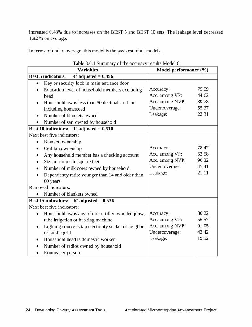
3.6 Model 6 This model excluded all monetary variables, leaving 153 variables in the analysis. The adjusted R-squared ranged from 0.456 to 0.536, i.e., lower in all sets than in the previous models. As in the previous model, this model incorporates a high proportion of asset and housing-related variables. The best performance was observed in the BEST 15 set, with an accuracy of 80.22 % —slightly lower than the highest accuracy from the previous model (80.35 %). While the accuracy level among the very poor decreased by 2.38% in average, the accuracy among the not very poor
24 Developing Poverty Assessment Tools Accelerated Microenterprise Advancement Project
increased 0.48% due to increases on the BEST 5 and BEST 10 sets. The leakage level decreased 1.82 % on average. In terms of undercoverage, this model is the weakest of all models.
Table 3.6.1 Summary of the accuracy results Model 6 Variables Model performance (%)
Best 5 indicators: R2 adjusted = 0.456 • Key or security lock in main entrance door • Education level of household members excluding
head • Household owns less than 50 decimals of land
including homestead • Number of blankets owned • Number of sari owned by household
Accuracy: Acc. among VP: Acc. among NVP: Undercoverage: Leakage:
75.59 44.62 89.78 55.37 22.31
Best 10 indicators: R2 adjusted = 0.510 Next best five indicators:
• Blanket ownership • Ceil fan ownership • Any household member has a checking account • Size of rooms in square feet • Number of milk cows owned by household • Dependency ratio: younger than 14 and older than
60 years Removed indicators:
• Number of blankets owned
Accuracy: Acc. among VP: Acc. among NVP: Undercoverage: Leakage:
78.47 52.58 90.32 47.41 21.11
Best 15 indicators: R2 adjusted = 0.536 Next best five indicators:
• Household owns any of motor tiller, wooden plow, tube irrigation or husking machine
• Lighting source is tap electricity socket of neighbor or public grid
• Household head is domestic worker • Number of radios owned by household • Rooms per person
Accuracy: Acc. among VP: Acc. among NVP: Undercoverage: Leakage:
80.22 56.57 91.05 43.42 19.52
Results from regression models 25
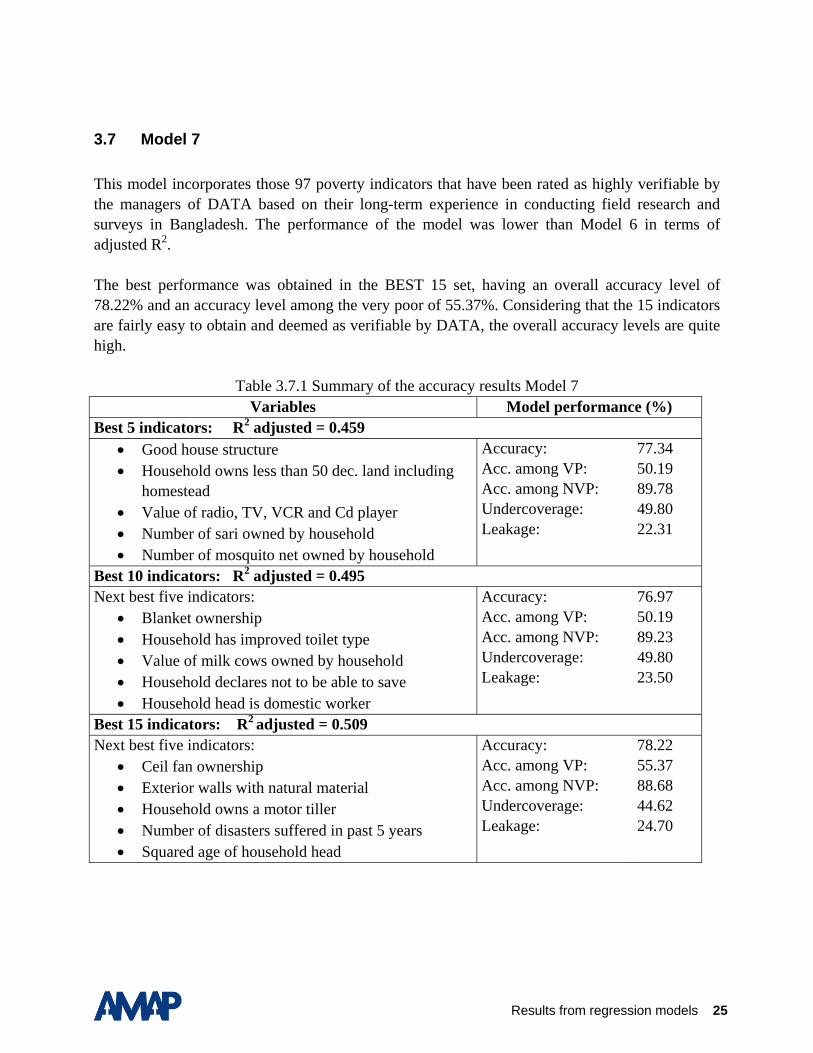
3.7 Model 7 This model incorporates those 97 poverty indicators that have been rated as highly verifiable by the managers of DATA based on their long-term experience in conducting field research and surveys in Bangladesh. The performance of the model was lower than Model 6 in terms of adjusted R2. The best performance was obtained in the BEST 15 set, having an overall accuracy level of 78.22% and an accuracy level among the very poor of 55.37%. Considering that the 15 indicators are fairly easy to obtain and deemed as verifiable by DATA, the overall accuracy levels are quite high.
Table 3.7.1 Summary of the accuracy results Model 7 Variables Model performance (%)
Best 5 indicators: R2 adjusted = 0.459 • Good house structure • Household owns less than 50 dec. land including
homestead • Value of radio, TV, VCR and Cd player • Number of sari owned by household • Number of mosquito net owned by household
Accuracy: Acc. among VP: Acc. among NVP: Undercoverage: Leakage:
77.34 50.19 89.78 49.80 22.31
Best 10 indicators: R2 adjusted = 0.495 Next best five indicators:
• Blanket ownership • Household has improved toilet type • Value of milk cows owned by household • Household declares not to be able to save • Household head is domestic worker
Accuracy: Acc. among VP: Acc. among NVP: Undercoverage: Leakage:
76.97 50.19 89.23 49.80 23.50
Best 15 indicators: R2 adjusted = 0.509 Next best five indicators:
• Ceil fan ownership • Exterior walls with natural material • Household owns a motor tiller • Number of disasters suffered in past 5 years • Squared age of household head
Accuracy: Acc. among VP: Acc. among NVP: Undercoverage: Leakage:
78.22 55.37 88.68 44.62 24.70

26 Developing Poverty Assessment Tools Accelerated Microenterprise Advancement Project
3.8 Model 8 This model is based on Model 7 but includes five additional regressors. Four of them are among the strongest indicators in the group of subjective variables, and the fifth one is the single predictor from the expenditure group. These variables are:
• Household feels that clothing expenses are below need • How much does the household need per month to live? • Days in past seven days with any of four superior food eaten • Position on the ladder of a household with 3600 Taka income per month and household
size = 5 • Clothing expenditure per capita in past 12 months
The incorporation of these variables increased the model’s performance to a level between Model 3 and Model 4. It can be observed that three of these new variables were selected already in the BEST 5 set, one was incorporated in the BEST 10 set and one more was included in the BEST 15 set. This situation reflects the importance of incorporating subjective variables within the models even though their verifiability may not be as easy as desired. The adjusted R-squared values ranged between 0.571 and 0.608. The best performance was achieved by the BEST15 set (81.22% overall accuracy). In comparison with Model 7, the overall accuracy increased on average by 3.38%. As well, the accuracy among the very poor increased on average 5.71% and the accuracy among the not very poor returned to a level above 90%. The degree of undercoverage ranged from 44.22 to 41.03% among the three sets, while the degree of leakage was stable around 18.4%.

Results from regression models 27
Table 3.8.1 Summary of the accuracy results Model 8
Variables Model performance (%) Best 5 indicators: R2 adjusted = 0.571
• Good house structure • Value of radio, TV, VCR and CD player • Household feels that clothing expenditures are
below need • Days in past 7 days with any of four superior food
eaten • Clothing expenditure per capita in past 12 months
Accuracy: Acc. among VP: Acc. among NVP: Undercoverage: Leakage:
80.35 55.77 91.60 44.22 18.32
Best 10 indicators: R2 adjusted = 0.598 Next best five indicators:
• Household owns less than 50 dec. land including homestead
• Value of milk cows owned by household • Number of ceil fans owned by household • Squared age of household head • How much does household need per month to live
Accuracy: Acc. among VP: Acc. among NVP: Undercoverage: Leakage:
81.10 58.16 91.60 41.83 18.32
Best 15 indicators: R2 adjusted = 0.608 Next best five indicators:
• Exterior walls with natural material • Number of cattle owned by household • Number of disasters suffered in past 5 years • Number of motor tiller owned by household • Position on the ladder of a household with 3600
Taka income per month and household size = 5
Accuracy: Acc. among VP: Acc. among NVP: Undercoverage: Leakage:
81.22 58.96 91.42 41.03 18.72
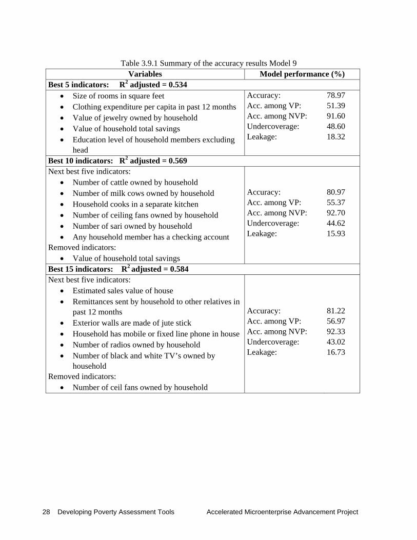
3.9 Model 9 Model 9 used a set of 114 regressors which are usually found in LSMS surveys from the World Bank. The model performed similar to model 4 in terms of overall accuracy and adjusted R-square. However, it had a lower performance in the accuracy levels among the very poor and among the not very poor, and therefore, higher degrees of undercoverage and leakage. The best performance was observed in the BEST 15 set, with 81.22% overall accuracy and 56.97% accuracy among the very poor. The leakage level was relatively low, which in consideration of the high level of accuracy among the very poor, suggests that this model may be more adequate for identifying the not very poor.
28 Developing Poverty Assessment Tools Accelerated Microenterprise Advancement Project
Table 3.9.1 Summary of the accuracy results Model 9
Variables Model performance (%) Best 5 indicators: R2 adjusted = 0.534
• Size of rooms in square feet • Clothing expenditure per capita in past 12 months • Value of jewelry owned by household • Value of household total savings • Education level of household members excluding
head
Accuracy: Acc. among VP: Acc. among NVP: Undercoverage: Leakage:
78.97 51.39 91.60 48.60 18.32
Best 10 indicators: R2 adjusted = 0.569 Next best five indicators:
• Number of cattle owned by household • Number of milk cows owned by household • Household cooks in a separate kitchen • Number of ceiling fans owned by household • Number of sari owned by household • Any household member has a checking account
Removed indicators: • Value of household total savings
Accuracy: Acc. among VP: Acc. among NVP: Undercoverage: Leakage:
80.97 55.37 92.70 44.62 15.93
Best 15 indicators: R2 adjusted = 0.584 Next best five indicators:
• Estimated sales value of house • Remittances sent by household to other relatives in
past 12 months • Exterior walls are made of jute stick • Household has mobile or fixed line phone in house • Number of radios owned by household • Number of black and white TV’s owned by
household Removed indicators:
• Number of ceil fans owned by household
Accuracy: Acc. among VP: Acc. among NVP: Undercoverage: Leakage:
81.22 56.97 92.33 43.02 16.73

Practitioner tools 29
Practitioner Tools
4.1 Loan size tool
4.1.1 Introduction
Loan size has been used in the past as an indicator of poverty (see Schreiner, 2001 and the Microenterprise Results Reporting database). In the following, we test this indicator, along with other variables, for accuracy in predicting the poverty status of borrowers13.
In the sample of 800 households, there are 345 households with adult members who are current clients of financial institutions. In these 345 households, a total of 476 adults had obtained a loan from a formal financial institution. The following table shows the type of institutions and their market share of the total of 476 clients, in absolute number of loans and percentage share.
Table 4.1.1.1 Share of clients according to type of financial institution
Type of organization Frequency Percentage
Public Bank (main or exclusive ownership by government) 138 29.0
Private Bank (main or exclusive ownership by private investor) 83 17.4
Cooperatives (main or exclusive ownership by members) 1 0.2
Top 45 MFI-NGOs in Bangladesh* 189 39.7
Other NGO providing microfinance service 42 8.8 Other governmental institution providing microfinance 19 4.0
Other governmental institution providing MF and business development service 1 0.2
Private firm or institution providing MF and business development service 3 0.6
Total 476 100.0 *As classified in MF Statistics by Credit and Development Forum Bangladesh.
4.1.2 Accuracy of indicators of loan size
In the survey we asked for the size of the first loan (see section I of composite questionnaire). As loan size usually progresses over time, we further asked about the size of the currently outstanding (not fully repaid) loans. If all loans were fully repaid at the time of the

30 Developing Poverty Assessment Tools Accelerated Microenterprise Advancement Project
survey, we asked about the size of the most recent loan.
The average values of loan size and total debt, by type of organization, are presented in the following table (n=345 households).
Table 4.1.2.1 Average loan size by type of financial institution
Type of financial institution
First loan: Average amount
borrowed, Taka
Most recent loan: Average
amount borrowed,
Taka
Maximum size of most recent
loan, Taka
Total outstanding
debt per household,
Taka (n=198)
Average size of outstanding loans, Taka
(n=198)
Top 45 NGOs in Bangladesh, and Grameen Bank (n =169) 4155 6766 7347 5107 3753 Other NGOs and civic institutions (n=31) 4399 8182 9094 4903 4112 Public bank or government credit program (n=119) 8254 10728 12343 10217 6671 Privately owned bank/ coops/other institutions (excl. Grameen Bank) (n=12) 5403 8240 8838 12238 11145 Total (n=345) 5745 8435 9435 6786 4913 Note: 1 US-Dollar is approx. 60 Taka (as of March/April 2004, time of survey).
In the sample of 800 households, there are 345 households having borrowed at least one time. Instead of presenting results from an ordinary least squares regression model over the sample of 345 households, we chose the more appropriate two-stage Heckman model: estimated in the first stage over 800 households (calculating the probability of being a borrower); and in the second stage testing each of the above indicators as a predictor of per-capita expenditures. The second stage in a Heckman model corrects for a potential selection bias, detecting a non-random pattern of who is a borrower and who is not. This selection bias was found highly significant. For example, households living in villages more distant from market and public institutions were significantly less likely to borrow. Among the three regressors for loan size, the best predictor was found to be the maximum size of most recent loans in the household. This indicator can be obtained by asking any borrowing household member about the size of the most recent loan, and – if there are multiple borrowers in a household – taking the value of the largest of these loans.
The following table shows the results of the best-fitted regression model, using the natural logarithm of the maximum size of most recent loans plus these control variables: household size, household size squared, age of household head, and four dummies for four out of five divisions. The regression is run with STATA as a two-stage regression model correcting for selection bias.
Practitioner tools 31
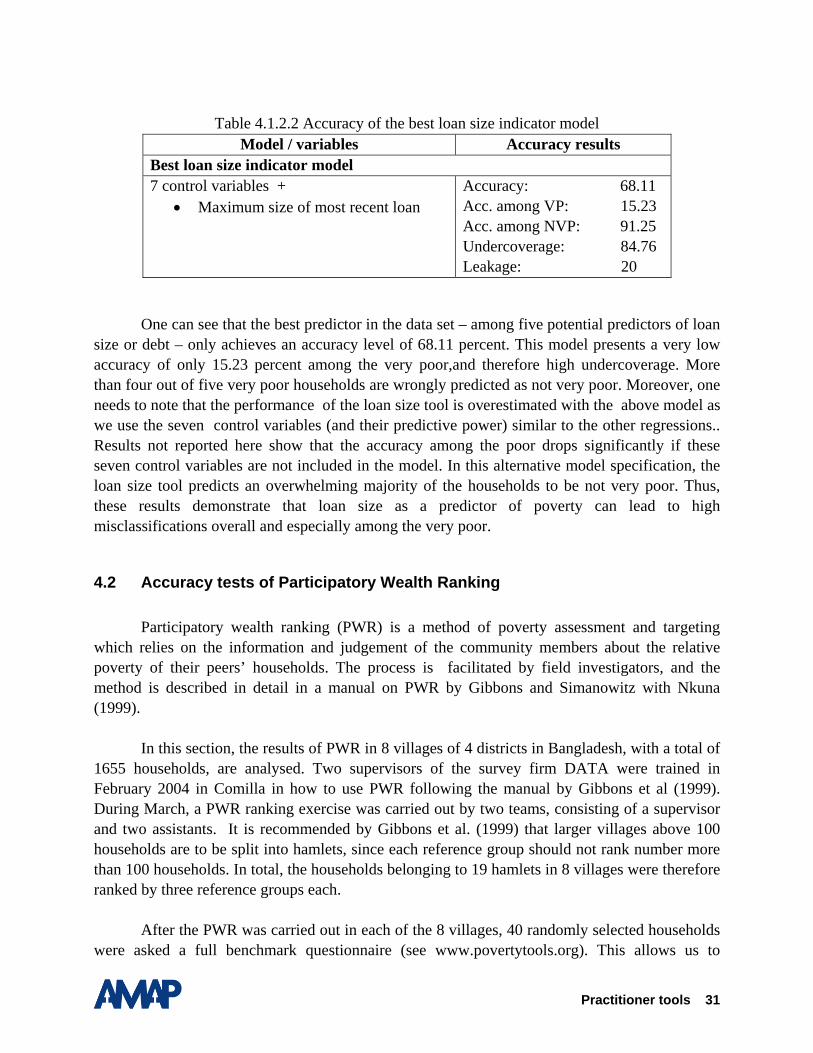
Table 4.1.2.2 Accuracy of the best loan size indicator model
Model / variables Accuracy results Best loan size indicator model 7 control variables +
• Maximum size of most recent loan Accuracy: 68.11 Acc. among VP: 15.23 Acc. among NVP: 91.25 Undercoverage: 84.76 Leakage: 20
One can see that the best predictor in the data set – among five potential predictors of loan
size or debt – only achieves an accuracy level of 68.11 percent. This model presents a very low accuracy of only 15.23 percent among the very poor,and therefore high undercoverage. More than four out of five very poor households are wrongly predicted as not very poor. Moreover, one needs to note that the performance of the loan size tool is overestimated with the above model as we use the seven control variables (and their predictive power) similar to the other regressions.. Results not reported here show that the accuracy among the poor drops significantly if these seven control variables are not included in the model. In this alternative model specification, the loan size tool predicts an overwhelming majority of the households to be not very poor. Thus, these results demonstrate that loan size as a predictor of poverty can lead to high misclassifications overall and especially among the very poor.
4.2 Accuracy tests of Participatory Wealth Ranking
Participatory wealth ranking (PWR) is a method of poverty assessment and targeting which relies on the information and judgement of the community members about the relative poverty of their peers’ households. The process is facilitated by field investigators, and the method is described in detail in a manual on PWR by Gibbons and Simanowitz with Nkuna (1999).
In this section, the results of PWR in 8 villages of 4 districts in Bangladesh, with a total of 1655 households, are analysed. Two supervisors of the survey firm DATA were trained in February 2004 in Comilla in how to use PWR following the manual by Gibbons et al (1999). During March, a PWR ranking exercise was carried out by two teams, consisting of a supervisor and two assistants. It is recommended by Gibbons et al. (1999) that larger villages above 100 households are to be split into hamlets, since each reference group should not rank number more than 100 households. In total, the households belonging to 19 hamlets in 8 villages were therefore ranked by three reference groups each.
After the PWR was carried out in each of the 8 villages, 40 randomly selected households were asked a full benchmark questionnaire (see www.povertytools.org). This allows us to

32 Developing Poverty Assessment Tools Accelerated Microenterprise Advancement Project
calculate – for each of the 320 households – a daily per-capita expenditure. These 320 households are a subset of the 799 sample households that were analyzed in Chapter 3. On the basis of this information, the 320 households were categorized as either to be very poor or not very poor.
The following analysis14 investigates how accurate the PWR scores are in predicting the poverty status of a household. Section 4.2.1 investigates the quality of the data on participatory wealth ranking, following the criteria provided by Gibbons et al. (1999). Section 4.2.2 presents the results for the whole sample first, and then searches for the so-called BEST score. The BEST score is defined as the average score from the three reference groups which achieve the highest overall accuracy in predicting the very poor and not very poor15. In this section, we further simulate by how much accuracy improves if we consider two subsamples, one with fairly consistent scores and another with highly consistent scores. Section 4.2.3 examines by how much accuracy will increase if the BEST score is calibrated to smaller geographical units, i.e., to the 4 sample districts, the 8 survey villages, and finally to the 19 hamlets. Section 4.2.4 summarizes the results.
4.2.1. Quality of the data from Participatory Wealth Ranking
Scores from PWR range between any positive number and the maximum score 100. A higher score means more poverty – relative to the other community members. As explained in the PWR manual, three reference groups each assign a score to each household belonging to the community.
Each household in a hamlet was given a PWR score by three independent reference groups. A reference group consists of several women volunteers being members of the hamlet in which the PWR is carried out. Following Gibbons and Simanowitz with Nkuna (1999), a set of three scores given by three independent reference groups is considered consistent, if the difference between any of the three scores is 25 or less. In Table 4.2.1.1a and 4.2.1.1b below, the third column shows the percentage of households that are consistently scored. Table 4.2.1.1a refers to all 1655 households in the 8 villages, whereas Table 4.2.1.1b refers only to the 320 survey households for which the benchmark expenditure data is available. Column 2 shows the percentage of households for which two of the three scores are within the limit of 25, while with the third score differs from the other by less than 50. Scores as shown in Column 2 are good, and can be used directly for wealth ranking.
When only one of the three scores matches by a difference of 25, it means that the difference with respect to the other scores could be in the range from above 25 to less than 50 or from 50 and above. In the former case (see column 1b), this somewhat inconsistent score can still be averaged with the other two scores (see Gibbons et al. (1999)). In the latter case, however, a difference of 50 and above is considered to be highly inconsistent by Gibbons et al. (1999), and any score creating a difference of 50 and above with the other scores should not be used for analysis. In Table 4.2.1.1a and 4.2.1.1b below, column 1 shows the percentage of sets that have none or only one out of three scores that match by a difference of 25 or less. In column 1a, the
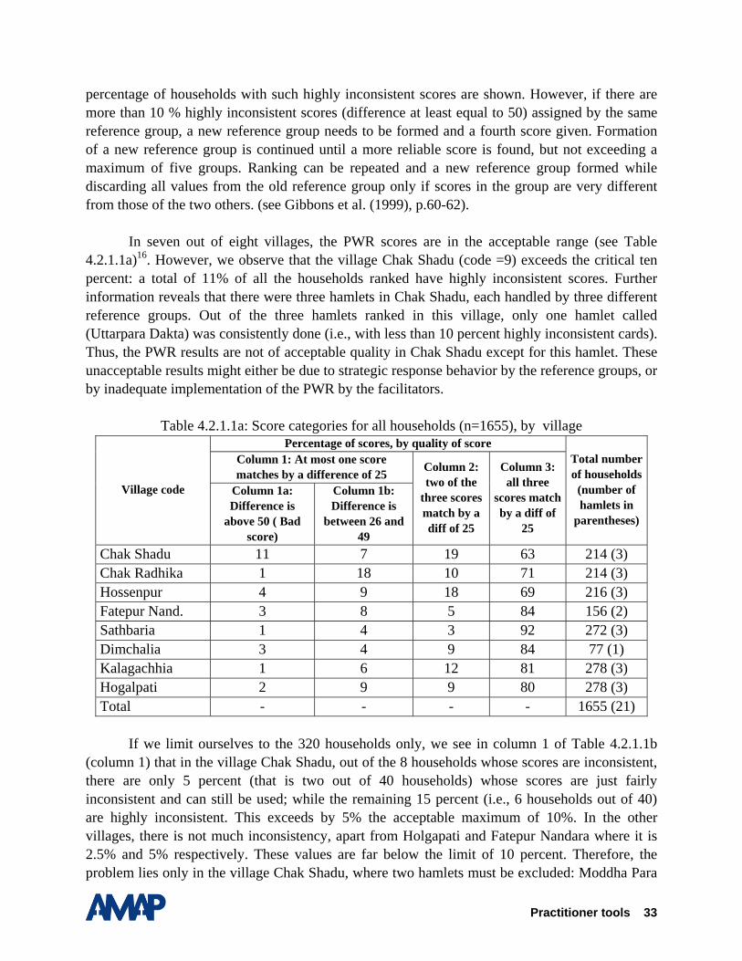
Practitioner tools 33
percentage of households with such highly inconsistent scores are shown. However, if there are more than 10 % highly inconsistent scores (difference at least equal to 50) assigned by the same reference group, a new reference group needs to be formed and a fourth score given. Formation of a new reference group is continued until a more reliable score is found, but not exceeding a maximum of five groups. Ranking can be repeated and a new reference group formed while discarding all values from the old reference group only if scores in the group are very different from those of the two others. (see Gibbons et al. (1999), p.60-62).
In seven out of eight villages, the PWR scores are in the acceptable range (see Table 4.2.1.1a)16. However, we observe that the village Chak Shadu (code =9) exceeds the critical ten percent: a total of 11% of all the households ranked have highly inconsistent scores. Further information reveals that there were three hamlets in Chak Shadu, each handled by three different reference groups. Out of the three hamlets ranked in this village, only one hamlet called (Uttarpara Dakta) was consistently done (i.e., with less than 10 percent highly inconsistent cards). Thus, the PWR results are not of acceptable quality in Chak Shadu except for this hamlet. These unacceptable results might either be due to strategic response behavior by the reference groups, or by inadequate implementation of the PWR by the facilitators.
Table 4.2.1.1a: Score categories for all households (n=1655), by village Percentage of scores, by quality of score
Column 1: At most one score matches by a difference of 25
Village code Column 1a: Difference is
above 50 ( Bad score)
Column 1b: Difference is
between 26 and 49
Column 2: two of the
three scores match by a diff of 25
Column 3: all three
scores match by a diff of
25
Total number of households
(number of hamlets in
parentheses)
Chak Shadu 11 7 19 63 214 (3) Chak Radhika 1 18 10 71 214 (3) Hossenpur 4 9 18 69 216 (3) Fatepur Nand. 3 8 5 84 156 (2) Sathbaria 1 4 3 92 272 (3) Dimchalia 3 4 9 84 77 (1) Kalagachhia 1 6 12 81 278 (3) Hogalpati 2 9 9 80 278 (3) Total - - - - 1655 (21)
If we limit ourselves to the 320 households only, we see in column 1 of Table 4.2.1.1b
(column 1) that in the village Chak Shadu, out of the 8 households whose scores are inconsistent, there are only 5 percent (that is two out of 40 households) whose scores are just fairly inconsistent and can still be used; while the remaining 15 percent (i.e., 6 households out of 40) are highly inconsistent. This exceeds by 5% the acceptable maximum of 10%. In the other villages, there is not much inconsistency, apart from Holgapati and Fatepur Nandara where it is 2.5% and 5% respectively. These values are far below the limit of 10 percent. Therefore, the problem lies only in the village Chak Shadu, where two hamlets must be excluded: Moddha Para
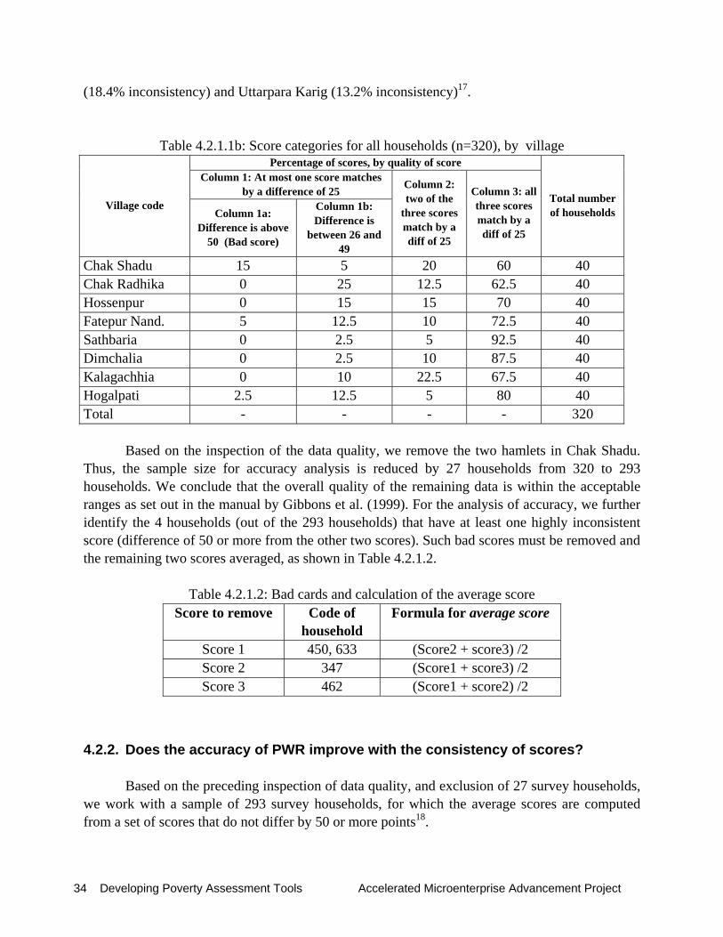
34 Developing Poverty Assessment Tools Accelerated Microenterprise Advancement Project
(18.4% inconsistency) and Uttarpara Karig (13.2% inconsistency)17.
Table 4.2.1.1b: Score categories for all households (n=320), by village Percentage of scores, by quality of score
Column 1: At most one score matches by a difference of 25
Village code Column 1a:
Difference is above 50 (Bad score)
Column 1b: Difference is
between 26 and 49
Column 2: two of the
three scores match by a diff of 25
Column 3: all three scores match by a diff of 25
Total number of households
Chak Shadu 15 5 20 60 40 Chak Radhika 0 25 12.5 62.5 40 Hossenpur 0 15 15 70 40 Fatepur Nand. 5 12.5 10 72.5 40 Sathbaria 0 2.5 5 92.5 40 Dimchalia 0 2.5 10 87.5 40 Kalagachhia 0 10 22.5 67.5 40 Hogalpati 2.5 12.5 5 80 40 Total - - - - 320
Based on the inspection of the data quality, we remove the two hamlets in Chak Shadu. Thus, the sample size for accuracy analysis is reduced by 27 households from 320 to 293 households. We conclude that the overall quality of the remaining data is within the acceptable ranges as set out in the manual by Gibbons et al. (1999). For the analysis of accuracy, we further identify the 4 households (out of the 293 households) that have at least one highly inconsistent score (difference of 50 or more from the other two scores). Such bad scores must be removed and the remaining two scores averaged, as shown in Table 4.2.1.2.
Table 4.2.1.2: Bad cards and calculation of the average score Score to remove Code of
household Formula for average score
Score 1 450, 633 (Score2 + score3) /2 Score 2 347 (Score1 + score3) /2 Score 3 462 (Score1 + score2) /2
4.2.2. Does the accuracy of PWR improve with the consistency of scores?
Based on the preceding inspection of data quality, and exclusion of 27 survey households, we work with a sample of 293 survey households, for which the average scores are computed from a set of scores that do not differ by 50 or more points18.

Practitioner tools 35
Determining the accuracy of PWR is done through a simulation exercise. We choose an arbitrary value for the average score (say 80), and assume that our ‘PWR Poverty Assessment tool’ is defined as predicting every household with an average PWR score with a value below 80 as not very poor. Similarly, our tool predicts every household having a score of 80 or more as being very poor.
Thus, in this example, the poverty assessment tool based on PWR data would then be defined as: Any household having an average score of 80 or above is rated as very poor, otherwise not very poor.
We then use this tool to calculate the predicted percentages for very poor and not very poor, and compare these with the actual very poor and not very poor (as defined by the benchmark expenditures). For example, in Table 4.2.2.1, for the PWR tool with a cut-off score of 80, we obtain an overall accuracy of 67.6 percent for the sample of 293 households. For this cut-off value, we also present the other four performance measures.
Table 4.2.2.1 presents the performance measures for the entire range of PWR scores that are observed in the sample. These results are obtained by calculating the performance measures for alternative tools using the entire range of PWR scores observed in the sample. Thus, when iterating in a stepwise fashion through the entire observed range of PWR scores, accuracy levels and measures of undercoverage and leakage are calculated for a set of alternatively calibrated PWR tools. One can then identify what we term the best score, i.e., the score that maximizes accuracy19. In Table 4.2.2.1, the BEST score is 100, and a PWR tool calibrated with the value 100 would yield the highest accuracy in the sample. This tool would achieve an overall accuracy of 70.3 percent, but produces a very low accuracy among the very poor of only 33 percent. In other words, two out of three households are misclassified. One can observe from the table that choosing a tool with a lower cut-off score (for example 80) would reduce overall accuracy, but improve the accuracy among the very poor.
Table 4.2.2.1 shows the variation of the five performance measures. The simulated range of the score ranges from 70 to 100. Within this range, accuracy increases, but – as expected – the accuracy among the very poor is falling while the accuracy among the not very poor is increasing. Table 4.2.2.1 Whole sample (n=293 households from 8 villages in 4 districts of Bangladesh)
Simulated score (in percent) 70 75 80 85 90 94 100 Overall accuracy 64.5 67.2 67.6 68.3 69.3 69.6 70.3 Accuracy among very poor 78.03 68.56 64.60 54.22 43.84 36.52 33.46 Accuracy among not very poor 57.91 66.54 69.06 75.16 81.71 85.72 88.25 Very poor wrongly predicted (undercoverage) 21.98 31.44 35.40 45.78 56.16 63.48 66.54 Not very poor wrongly predicted (leakage) 42.09 33.46 30.94 24.84 18.29 14.28 11.75
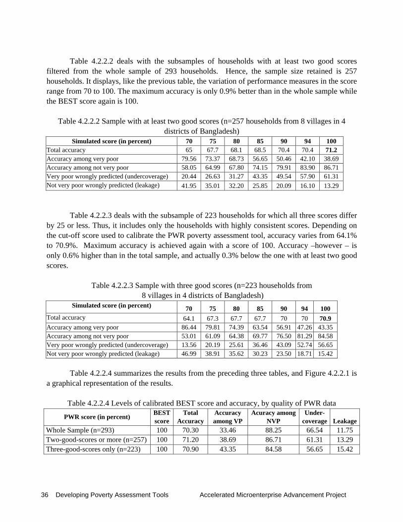
36 Developing Poverty Assessment Tools Accelerated Microenterprise Advancement Project
Table 4.2.2.2 deals with the subsamples of households with at least two good scores
filtered from the whole sample of 293 households. Hence, the sample size retained is 257 households. It displays, like the previous table, the variation of performance measures in the score range from 70 to 100. The maximum accuracy is only 0.9% better than in the whole sample while the BEST score again is 100.
Table 4.2.2.2 Sample with at least two good scores (n=257 households from 8 villages in 4 districts of Bangladesh)
Simulated score (in percent) 70 75 80 85 90 94 100 Total accuracy 65 67.7 68.1 68.5 70.4 70.4 71.2 Accuracy among very poor 79.56 73.37 68.73 56.65 50.46 42.10 38.69 Accuracy among not very poor 58.05 64.99 67.80 74.15 79.91 83.90 86.71 Very poor wrongly predicted (undercoverage) 20.44 26.63 31.27 43.35 49.54 57.90 61.31 Not very poor wrongly predicted (leakage) 41.95 35.01 32.20 25.85 20.09 16.10 13.29
Table 4.2.2.3 deals with the subsample of 223 households for which all three scores differ by 25 or less. Thus, it includes only the households with highly consistent scores. Depending on the cut-off score used to calibrate the PWR poverty assessment tool, accuracy varies from 64.1% to 70.9%. Maximum accuracy is achieved again with a score of 100. Accuracy –however – is only 0.6% higher than in the total sample, and actually 0.3% below the one with at least two good scores.
Table 4.2.2.3 Sample with three good scores (n=223 households from 8 villages in 4 districts of Bangladesh)
Simulated score (in percent) 70 75 80 85 90 94 100 Total accuracy 64.1 67.3 67.7 67.7 70 70 70.9 Accuracy among very poor 86.44 79.81 74.39 63.54 56.91 47.26 43.35 Accuracy among not very poor 53.01 61.09 64.38 69.77 76.50 81.29 84.58 Very poor wrongly predicted (undercoverage) 13.56 20.19 25.61 36.46 43.09 52.74 56.65 Not very poor wrongly predicted (leakage) 46.99 38.91 35.62 30.23 23.50 18.71 15.42
Table 4.2.2.4 summarizes the results from the preceding three tables, and Figure 4.2.2.1 is a graphical representation of the results.
Table 4.2.2.4 Levels of calibrated BEST score and accuracy, by quality of PWR data
PWR score (in percent) BEST score
Total Accuracy
Accuracy among VP
Acuracy among NVP
Under-coverage Leakage
Whole Sample (n=293) 100 70.30 33.46 88.25 66.54 11.75 Two-good-scores or more (n=257) 100 71.20 38.69 86.71 61.31 13.29 Three-good-scores only (n=223) 100 70.90 43.35 84.58 56.65 15.42
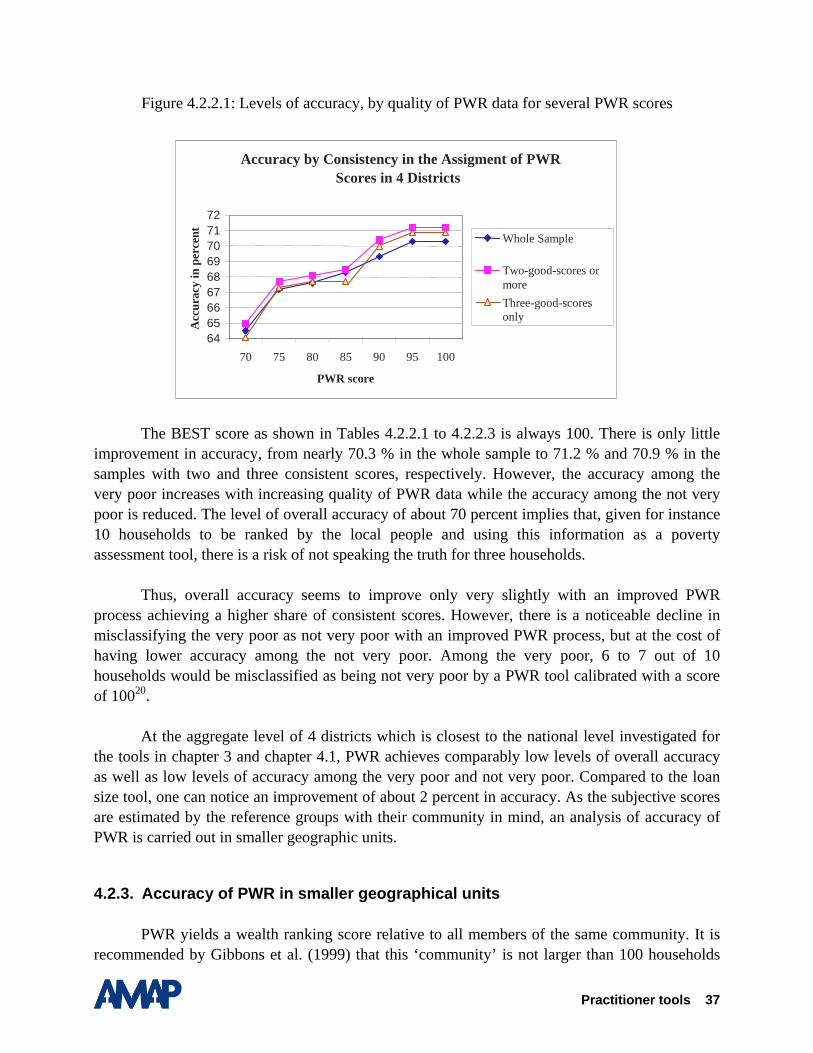
Practitioner tools 37
Figure 4.2.2.1: Levels of accuracy, by quality of PWR data for several PWR scores
The BEST score as shown in Tables 4.2.2.1 to 4.2.2.3 is always 100. There is only little
improvement in accuracy, from nearly 70.3 % in the whole sample to 71.2 % and 70.9 % in the samples with two and three consistent scores, respectively. However, the accuracy among the very poor increases with increasing quality of PWR data while the accuracy among the not very poor is reduced. The level of overall accuracy of about 70 percent implies that, given for instance 10 households to be ranked by the local people and using this information as a poverty assessment tool, there is a risk of not speaking the truth for three households.
Thus, overall accuracy seems to improve only very slightly with an improved PWR process achieving a higher share of consistent scores. However, there is a noticeable decline in misclassifying the very poor as not very poor with an improved PWR process, but at the cost of having lower accuracy among the not very poor. Among the very poor, 6 to 7 out of 10 households would be misclassified as being not very poor by a PWR tool calibrated with a score of 10020.
At the aggregate level of 4 districts which is closest to the national level investigated for the tools in chapter 3 and chapter 4.1, PWR achieves comparably low levels of overall accuracy as well as low levels of accuracy among the very poor and not very poor. Compared to the loan size tool, one can notice an improvement of about 2 percent in accuracy. As the subjective scores are estimated by the reference groups with their community in mind, an analysis of accuracy of PWR is carried out in smaller geographic units.
4.2.3. Accuracy of PWR in smaller geographical units
PWR yields a wealth ranking score relative to all members of the same community. It is recommended by Gibbons et al. (1999) that this ‘community’ is not larger than 100 households
Accuracy by Consistency in the Assigment of PWR
Scores in 4 Districts
64 65 66 67 68 69 70 71 72
70 75 80 85 90 95 100
PWR score
Acc
urac
y in
per
cent
Whole Sample
Two-good-scores or moreThree-good-scores only
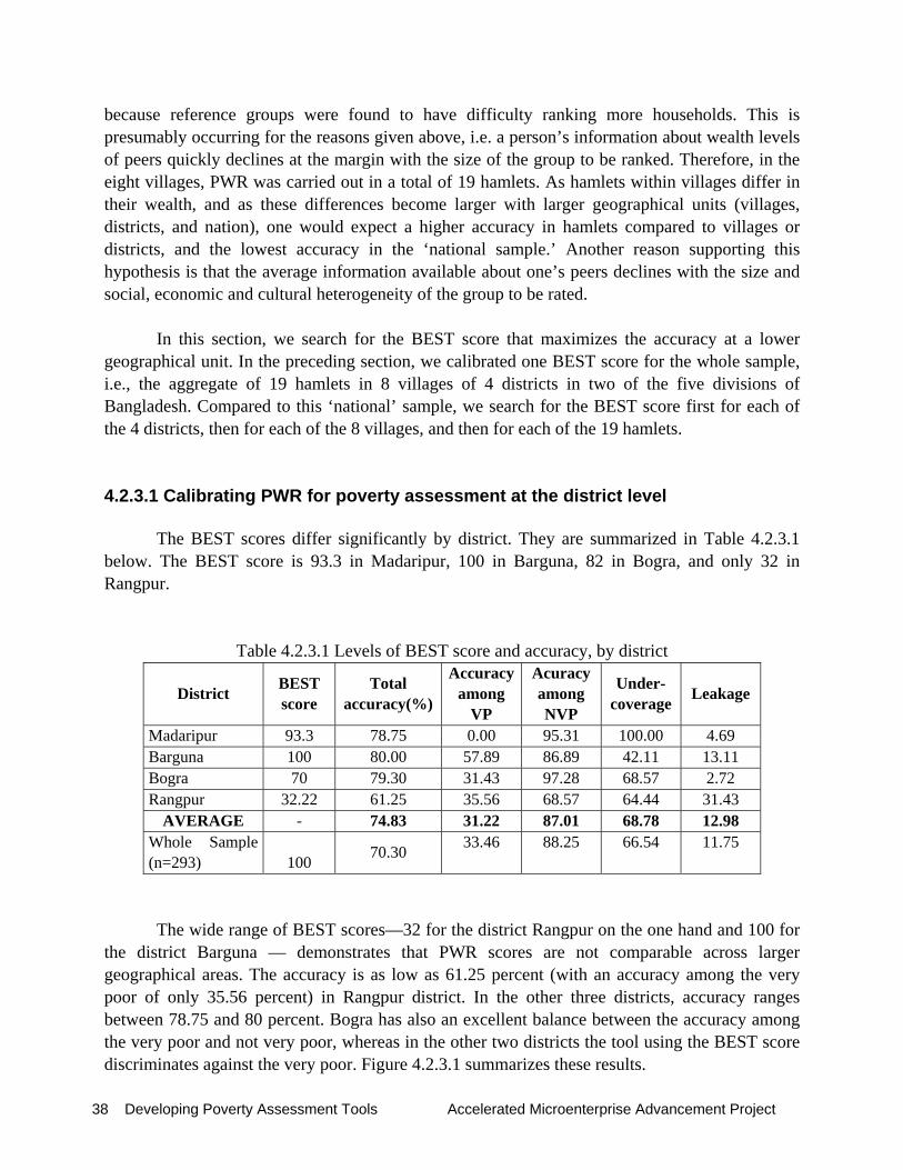
38 Developing Poverty Assessment Tools Accelerated Microenterprise Advancement Project
because reference groups were found to have difficulty ranking more households. This is presumably occurring for the reasons given above, i.e. a person’s information about wealth levels of peers quickly declines at the margin with the size of the group to be ranked. Therefore, in the eight villages, PWR was carried out in a total of 19 hamlets. As hamlets within villages differ in their wealth, and as these differences become larger with larger geographical units (villages, districts, and nation), one would expect a higher accuracy in hamlets compared to villages or districts, and the lowest accuracy in the ‘national sample.’ Another reason supporting this hypothesis is that the average information available about one’s peers declines with the size and social, economic and cultural heterogeneity of the group to be rated.
In this section, we search for the BEST score that maximizes the accuracy at a lower
geographical unit. In the preceding section, we calibrated one BEST score for the whole sample, i.e., the aggregate of 19 hamlets in 8 villages of 4 districts in two of the five divisions of Bangladesh. Compared to this ‘national’ sample, we search for the BEST score first for each of the 4 districts, then for each of the 8 villages, and then for each of the 19 hamlets. 4.2.3.1 Calibrating PWR for poverty assessment at the district level
The BEST scores differ significantly by district. They are summarized in Table 4.2.3.1 below. The BEST score is 93.3 in Madaripur, 100 in Barguna, 82 in Bogra, and only 32 in Rangpur.
Table 4.2.3.1 Levels of BEST score and accuracy, by district
District BEST score
Total accuracy(%)
Accuracy among
VP
Acuracy among NVP
Under-coverage Leakage
Madaripur 93.3 78.75 0.00 95.31 100.00 4.69 Barguna 100 80.00 57.89 86.89 42.11 13.11 Bogra 70 79.30 31.43 97.28 68.57 2.72 Rangpur 32.22 61.25 35.56 68.57 64.44 31.43
AVERAGE - 74.83 31.22 87.01 68.78 12.98 Whole Sample (n=293) 100 70.30 33.46 88.25 66.54 11.75
The wide range of BEST scores—32 for the district Rangpur on the one hand and 100 for the district Barguna — demonstrates that PWR scores are not comparable across larger geographical areas. The accuracy is as low as 61.25 percent (with an accuracy among the very poor of only 35.56 percent) in Rangpur district. In the other three districts, accuracy ranges between 78.75 and 80 percent. Bogra has also an excellent balance between the accuracy among the very poor and not very poor, whereas in the other two districts the tool using the BEST score discriminates against the very poor. Figure 4.2.3.1 summarizes these results.

Practitioner tools 39
Figure 4.2.3.1 Graphical representation of accuracy in the whole sample and in districts (n=293 households from 8 villages)
Accuracy in Districts and in the Whole Sample
25354555657585
32 70 75 80 85 90 94 95 100
Anchor score
Acc
urac
y Whole SampleMadripur (7)Barguna (8)Bogra(5)Rangpur (6)
4.2.3.2 Calibrating PWR for poverty assessment at the village and hamlet level
As expected, average accuracy of BEST scores in villages is still higher than in districts. From the summary table below we see that the accuracy of BEST score ranges between 65 percent and an excellent 90 percent in Holgapati.
Table 4.2.3.2 Levels of BEST score and accuracy, by village Village BEST
score Total
accuracy (%)
Accuracy among
VP
Accuracy among NVP
Under-coverage Leakage
Chak Shadu 93.33 84.6 0.0 91.7 100.0 8.3 Chak Radhika 70 82.5 86.7 80.0 13.3 20.0 Hossenpur 32.22 65.0 100.0 12.5 0.0 87.5 Fatepur Nandaram 87.78 65.0 71.4 57.9 28.6 42.1 Sathbaria 94.44 80.0 14.3 93.9 85.7 6.1 Dimchalia 93.33 80.0 33.3 93.5 66.7 6.5 Kalagachia 100 70.0 37.5 78.1 62.5 21.9 Hogalpati 100 90.0 72.7 96.1 27.3 3.4 Average - 77.14 51.99 75.46 48.01 24.48

40 Developing Poverty Assessment Tools Accelerated Microenterprise Advancement Project
A further increase in accuracy can be noticed if the PWR scores are calibrated at the hamlet level. The table below summarizes the results.
Table 4.2.3.2 Levels of BEST score and accuracy, by hamlets
Num-ber Hamlet Best score Accuracy Accuracy
among VP Acuracy
among NVP Under-
coverage Leakage
1 Moddha Para 68.33 57.1 60.0 55.5 40 44.5 2 Uttarpara,
Dakta 93.33 84.6 0.0 91.7 100 8.3
3 Uttarpara, karig 100 69.2 33.3 100.0 67.7 0.0 4 Chanundha para 71.11 76.9 87.5 60.0 12.5 40.0 5 Maddha para 71.67 or
73.33
84.6
75.0
88.9
25.0 11.1 6 Paschimpara 67.78 92.9 66.9 100.0 33.1 0.0 7 Fakirpara
(Pasch 18.89 or
32.22
78.6
100.0
25.1
0.0 74.9 8 Fakirpara
(Purbo 83.33 64.7 88.9 37.5 11.1
62.5 9 Uttarpara (Jangi 33.33 66.7 100.0 25.1 0.0 74.9 10 Kabirazpara 87.78 65 71.4 57.9 28.6 42.1 11 Paschimpara 80 or 100 72.2 0.1 92.8 99.9 7.2 12 Purbopara, Pasc 94.44 86.4 33.3 94.8 66.7 5.2 13 Dimchalia 86.7 or
93.33
80
33.3
93.5
66.7 6.5 14 Dakkhinpara 64.44 70 75.0 50.0 25.0 50.0 15 Paschimpara 87.78 or
100 81.8
not defined
81.8
not defined 18.2 16 Purbopara 100 73.7 74.8 73.4 25.2 26.6 17 Maddha P. 88.89 or
94.44 75
0.0
90.0
100.0 10.0 18 Purbopara Pasc 86.67 or
100 94.1
83.3
100.0
16.7 0.0 19 Purbopara Pd. 100 90.9 100.0 87.5 0.0 12.5 Average (19 hamlets, whole sample n=320)
77.08 60.16 73.97 39.90 26.03
Average excluding two hamlets of Chak Shadu ( n=293)
78.71 61.84 73.53 38.16 26.47
Note: Not defined means that this hamlet did not have any very poor people in the sample.
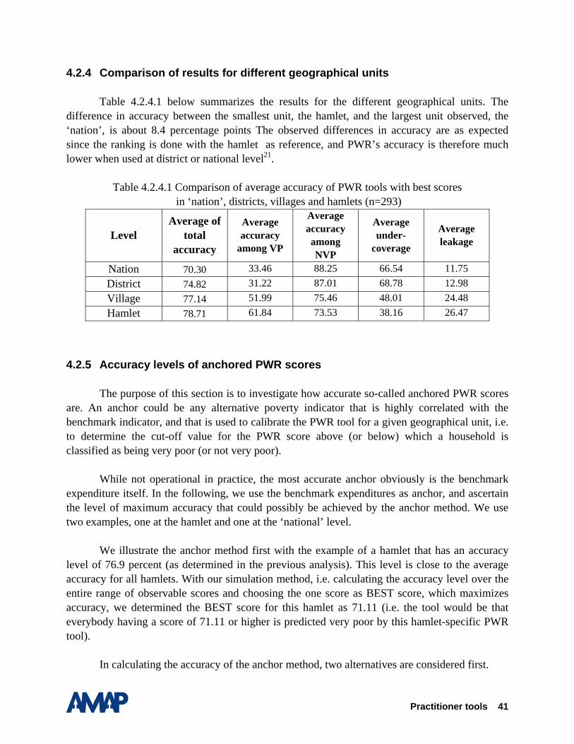
Practitioner tools 41
4.2.4 Comparison of results for different geographical units
Table 4.2.4.1 below summarizes the results for the different geographical units. The difference in accuracy between the smallest unit, the hamlet, and the largest unit observed, the ‘nation’, is about 8.4 percentage points The observed differences in accuracy are as expected since the ranking is done with the hamlet as reference, and PWR’s accuracy is therefore much lower when used at district or national level21.
Table 4.2.4.1 Comparison of average accuracy of PWR tools with best scores
in ‘nation’, districts, villages and hamlets (n=293)
Level Average of
total accuracy
Average accuracy
among VP
Average accuracy among NVP
Average under-
coverage
Average leakage
Nation 70.30 33.46 88.25 66.54 11.75 District 74.82 31.22 87.01 68.78 12.98 Village 77.14 51.99 75.46 48.01 24.48 Hamlet 78.71 61.84 73.53 38.16 26.47
4.2.5 Accuracy levels of anchored PWR scores
The purpose of this section is to investigate how accurate so-called anchored PWR scores are. An anchor could be any alternative poverty indicator that is highly correlated with the benchmark indicator, and that is used to calibrate the PWR tool for a given geographical unit, i.e. to determine the cut-off value for the PWR score above (or below) which a household is classified as being very poor (or not very poor).
While not operational in practice, the most accurate anchor obviously is the benchmark expenditure itself. In the following, we use the benchmark expenditures as anchor, and ascertain the level of maximum accuracy that could possibly be achieved by the anchor method. We use two examples, one at the hamlet and one at the ‘national’ level.
We illustrate the anchor method first with the example of a hamlet that has an accuracy level of 76.9 percent (as determined in the previous analysis). This level is close to the average accuracy for all hamlets. With our simulation method, i.e. calculating the accuracy level over the entire range of observable scores and choosing the one score as BEST score, which maximizes accuracy, we determined the BEST score for this hamlet as 71.11 (i.e. the tool would be that everybody having a score of 71.11 or higher is predicted very poor by this hamlet-specific PWR tool).
In calculating the accuracy of the anchor method, two alternatives are considered first.
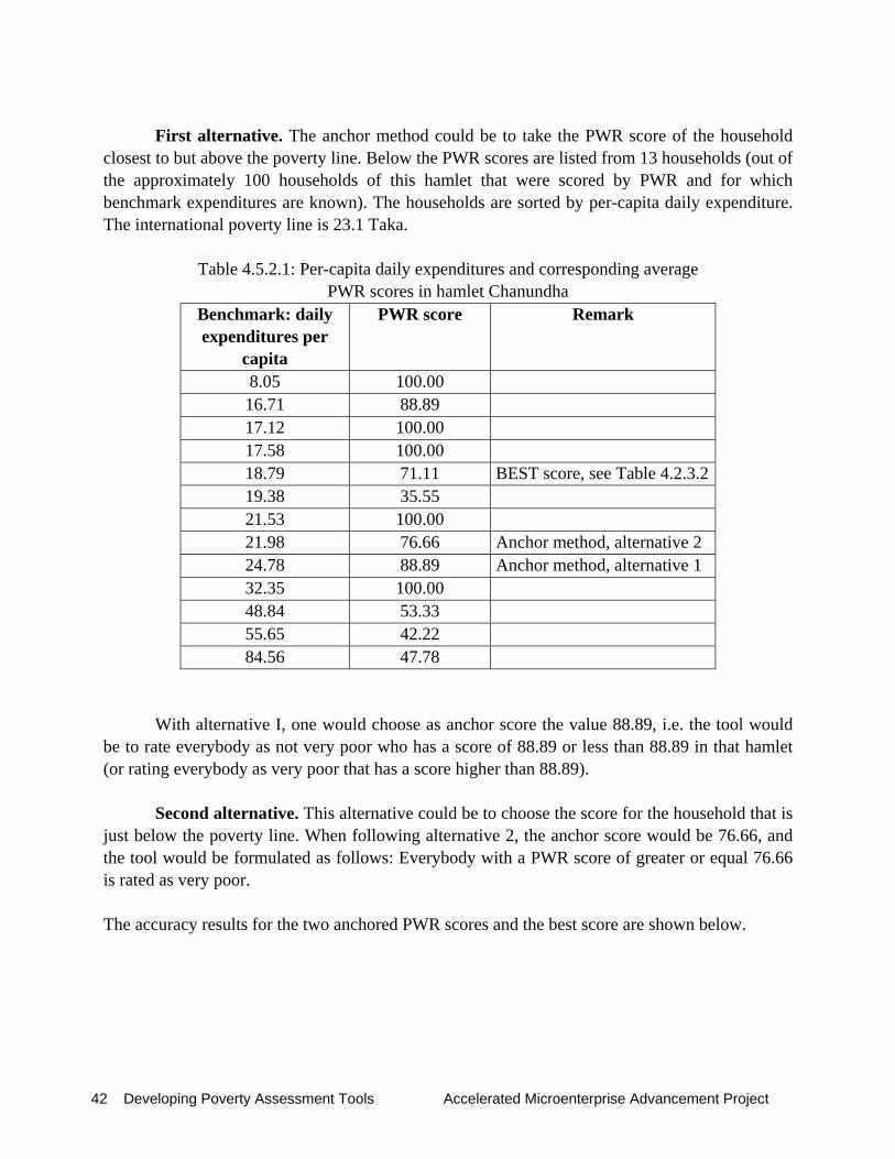
42 Developing Poverty Assessment Tools Accelerated Microenterprise Advancement Project
First alternative. The anchor method could be to take the PWR score of the household
closest to but above the poverty line. Below the PWR scores are listed from 13 households (out of the approximately 100 households of this hamlet that were scored by PWR and for which benchmark expenditures are known). The households are sorted by per-capita daily expenditure. The international poverty line is 23.1 Taka.
Table 4.5.2.1: Per-capita daily expenditures and corresponding average
PWR scores in hamlet Chanundha Benchmark: daily expenditures per
capita
PWR score Remark
8.05 100.00 16.71 88.89 17.12 100.00 17.58 100.00 18.79 71.11 BEST score, see Table 4.2.3.2 19.38 35.55 21.53 100.00 21.98 76.66 Anchor method, alternative 2 24.78 88.89 Anchor method, alternative 1 32.35 100.00 48.84 53.33 55.65 42.22 84.56 47.78
With alternative I, one would choose as anchor score the value 88.89, i.e. the tool would be to rate everybody as not very poor who has a score of 88.89 or less than 88.89 in that hamlet (or rating everybody as very poor that has a score higher than 88.89).
Second alternative. This alternative could be to choose the score for the household that is just below the poverty line. When following alternative 2, the anchor score would be 76.66, and the tool would be formulated as follows: Everybody with a PWR score of greater or equal 76.66 is rated as very poor. The accuracy results for the two anchored PWR scores and the best score are shown below.
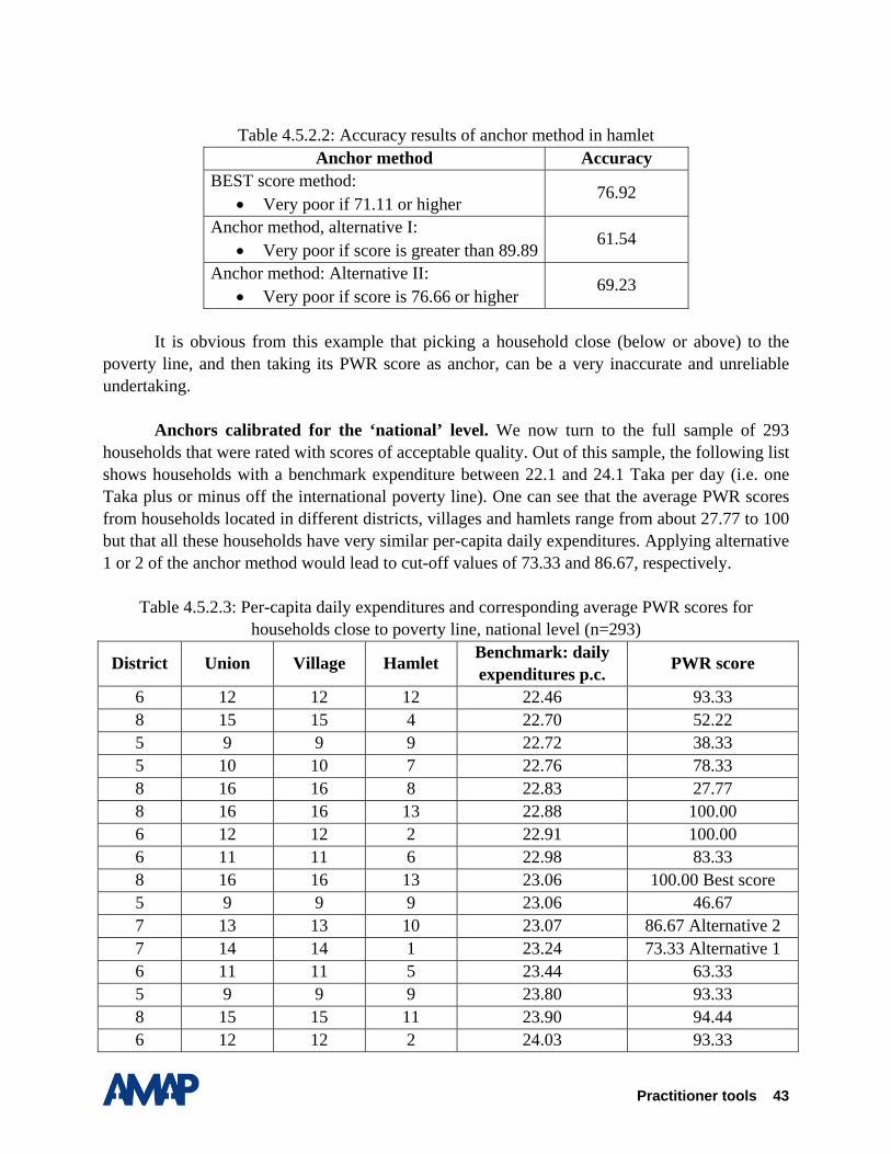
Practitioner tools 43
Table 4.5.2.2: Accuracy results of anchor method in hamlet
Anchor method Accuracy BEST score method:
• Very poor if 71.11 or higher 76.92
Anchor method, alternative I: • Very poor if score is greater than 89.89
61.54
Anchor method: Alternative II: • Very poor if score is 76.66 or higher
69.23
It is obvious from this example that picking a household close (below or above) to the
poverty line, and then taking its PWR score as anchor, can be a very inaccurate and unreliable undertaking.
Anchors calibrated for the ‘national’ level. We now turn to the full sample of 293 households that were rated with scores of acceptable quality. Out of this sample, the following list shows households with a benchmark expenditure between 22.1 and 24.1 Taka per day (i.e. one Taka plus or minus off the international poverty line). One can see that the average PWR scores from households located in different districts, villages and hamlets range from about 27.77 to 100 but that all these households have very similar per-capita daily expenditures. Applying alternative 1 or 2 of the anchor method would lead to cut-off values of 73.33 and 86.67, respectively.
Table 4.5.2.3: Per-capita daily expenditures and corresponding average PWR scores for households close to poverty line, national level (n=293)
District Union Village Hamlet Benchmark: daily expenditures p.c. PWR score
6 12 12 12 22.46 93.33 8 15 15 4 22.70 52.22 5 9 9 9 22.72 38.33 5 10 10 7 22.76 78.33 8 16 16 8 22.83 27.77 8 16 16 13 22.88 100.00 6 12 12 2 22.91 100.00 6 11 11 6 22.98 83.33 8 16 16 13 23.06 100.00 Best score 5 9 9 9 23.06 46.67 7 13 13 10 23.07 86.67 Alternative 2 7 14 14 1 23.24 73.33 Alternative 1 6 11 11 5 23.44 63.33 5 9 9 9 23.80 93.33 8 15 15 11 23.90 94.44 6 12 12 2 24.03 93.33

44 Developing Poverty Assessment Tools Accelerated Microenterprise Advancement Project
Table 4.5.2.4: Accuracy results of anchor method at ‘national’ level (n=293) Anchor method Accuracy
BEST score method: • Very poor if 100 or higher
70.3
Anchor method, alternative 1: • Very poor if score is greater than 73.33
65.3
Anchor method: Alternative 2: • Very poor if score is 86.67 or higher
67.7
Anchor method: Alternative 3: • Very poor if score is 83.44 or higher
66,3
A third alternative is to take the mean of households hovering around the poverty line.
This is simulated for example by taking the mean PWR score of the 5 closest households above or below the poverty line. The mean is 83.44, and the tool would be to rate a household as being very poor if the score is 83.44 or higher.
The comparison of accuracy results for the national level show that the anchor method –even if using the best possible, but in practice not applicable anchor – achieves accuracy levels at the ‘national’ level that fall below those associated with the loan size tool. If one uses an operational, but more inaccurate anchor, the levels of accuracy achieved by the anchor method will be lower as the ones displayed in Table 4.5.2.4 where benchmark expenditures as the perfect anchor are used.
4.2.6 Conclusion
The PWR data are of good quality, except for two hamlets that were excluded from the analysis of accuracy. The data from 293 households follow the criteria prescribed by Gibbons and Simanowitz with Nkuna (1999, p.60-62). The analysis results are as follows:
The results show that PWR achieves relatively low accuracy levels if used for assessing the poverty level of people living in larger geographic units. Note that the scales at the hamlet level are subjectively established, and whether a reference group distinguishes four or six wealth-differentiated groups of people in their hamlet is up to them. Moreover, their frame of reference are the people of the hamlet to be rated. Thus, the subjective scales of PWR cannot be compared across larger geographic units without accepting large reductions in accuracy and corresponding increases in leakage and undercoverage.
The results suggest that PWR is a fairly accurate targeting tool to reach the poorest if and when used in hamlets or villages, but not for larger geographic areas such as districts or the nation. Thus, the validity of PWR as a poverty targeting tool is confirmed if it is used at the village or hamlet level. The results further confirm the theoretical expectation that subjective
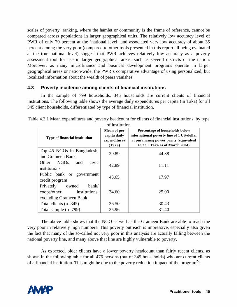
Practitioner tools 45
scales of poverty ranking, where the hamlet or community is the frame of reference, cannot be compared across populations in larger geographical units. The relatively low accuracy level of PWR of only 70 percent at the ‘national level’ and associated very low accuracy of about 35 percent among the very poor (compared to other tools presented in this report all being evaluated at the true national level) suggest that PWR achieves relatively low accuracy as a poverty assessment tool for use in larger geographical areas, such as several districts or the nation. Moreover, as many microfinance and business development programs operate in larger geographical areas or nation-wide, the PWR’s comparative advantage of using personalized, but localized information about the wealth of peers vanishes.
4.3 Poverty incidence among clients of financial institutions In the sample of 799 households, 345 households are current clients of financial
institutions. The following table shows the average daily expenditures per capita (in Taka) for all 345 client households, differentiated by type of financial institution. Table 4.3.1 Mean expenditures and poverty headcount for clients of financial institutions, by type
of institution
Type of financial institution
Mean of per capita daily
expenditures (Taka)
Percentage of households below international poverty line of 1 US-dollar at purchasing power parity (equivalent
to 23.1 Taka as of March 2004) Top 45 NGOs in Bangladesh, and Grameen Bank 29.89 44.38
Other NGOs and civic institutions 42.89 11.11
Public bank or government credit program 43.65 17.97
Privately owned bank/ coops/other institutions, excluding Grameen Bank
34.60 25.00
Total clients (n=345) 36.50 30.43 Total sample (n=799) 35.96 31.40
The above table shows that the NGO as well as the Grameen Bank are able to reach the
very poor in relatively high numbers. This poverty outreach is impressive, especially also given the fact that many of the so-called not very poor in this analysis are actually falling between the national poverty line, and many above that line are highly vulnerable to poverty.
As expected, older clients have a lower poverty headcount than fairly recent clients, as shown in the following table for all 476 persons (out of 345 households) who are current clients of a financial institution. This might be due to the poverty reduction impact of the program22.

46 Developing Poverty Assessment Tools Accelerated Microenterprise Advancement Project
Table 4.3.2 Poverty incidence of clients of financial institution, by years of being a client
Years of being a client
Mean of per capita daily
expenditures (Taka)
Percentage of households below international poverty line of 1 US-dollar
at purchasing power parity (equivalent to 23.1 Taka as of March 2004)
Less than one year
34.62 30.34
One to less than 6 years 35.09 31.30 Six to less than 11 years 41.58 18.95 More than 11 years 44.86 14.52 Total (n=476) 37.57 26.47
These results for Bangladesh suggest that it may be necessary to undertake poverty
assessments only on in-coming clients or new clients. Otherwise, successful programs that have targeted the poor in the past and have raised their living standards may be penalized, which appears much in opposite to the spirit driving the legislation regarding the development and certification of poverty assessment tools.

Summary 47
Summary
In this report, we reviewed two practitioner tools and presented 9 regression models, each
with a set of best 5, best 10, and best 15 regressors. Thus, in total, there are 27 potential, newly developed tools that could be used for poverty assessment in Bangladesh. Other tools can be generated from the data set by varying the choice of subsets of regressors, e.g. by using additional information on the difficulty or verifiability of indicators.
These few introductory sentences raise the question: What determines the choice of an appropriate practitioner tool? Before we turn to two issues related to this question, we briefly summarize the major results of the 9 models, critically evaluate the inaccuracies in prediction, and suggest a way forward in improving on the results.
5.1 Brief synthesis of results
The nine models show quite satisfactory levels of overall accuracy, i.e., the percentage of very poor or not very poor is correctly predicted. In the case of tools using only 5 poverty indicators (i.e., the BEST 5 models presented in chapter 3), levels in overall accuracy range from 75.59 percent for Model 6 (which has a restrictive set of regressors by excluding subjective and monetary variables) to 83.85 percent in Model 1 (which includes the full set of 253 regressors).
We further measured the accuracy of loan size, a commonly used indicator. The loan size tool yields an overall accuracy of only 68.1 percent. Finally, we assessed the accuracy of Participatory Wealth Ranking, and showed that PWR achieves an accuracy of 78.7 percent at the hamlet level. The results thus confirm the usefulness of PWR for accurately targeting the poorest in a given hamlet or community. At the aggregate geographic level covering several districts of Bangladesh, however, PWR achieved an accuracy of only 70.3 percent. This is only 2.2 percent more than the loan size tool as base comparator —which is a relatively low-cost and very practical tool for micro-finance institutions. This aggregate level, however, is the relevant geographical unit of comparison, since the poverty assessment tools are to be used across larger geographical areas as micro-finance and BDS programs supported by USAID operate in several districts of a country, if not nation-wide. In such larger geographical units, PWR as a poverty assessment tool achieves a fairly low accuracy rate, with very high undercoverage and leakage levels. The PWR tool could be calibrated with a lower cut-off score so as to reduce undercoverage and to increase accuracy among the very poor. However, such a re-calibration comes with a worsening performance with respect to total accuracy, leakage as well as accuracy among the not very poor.
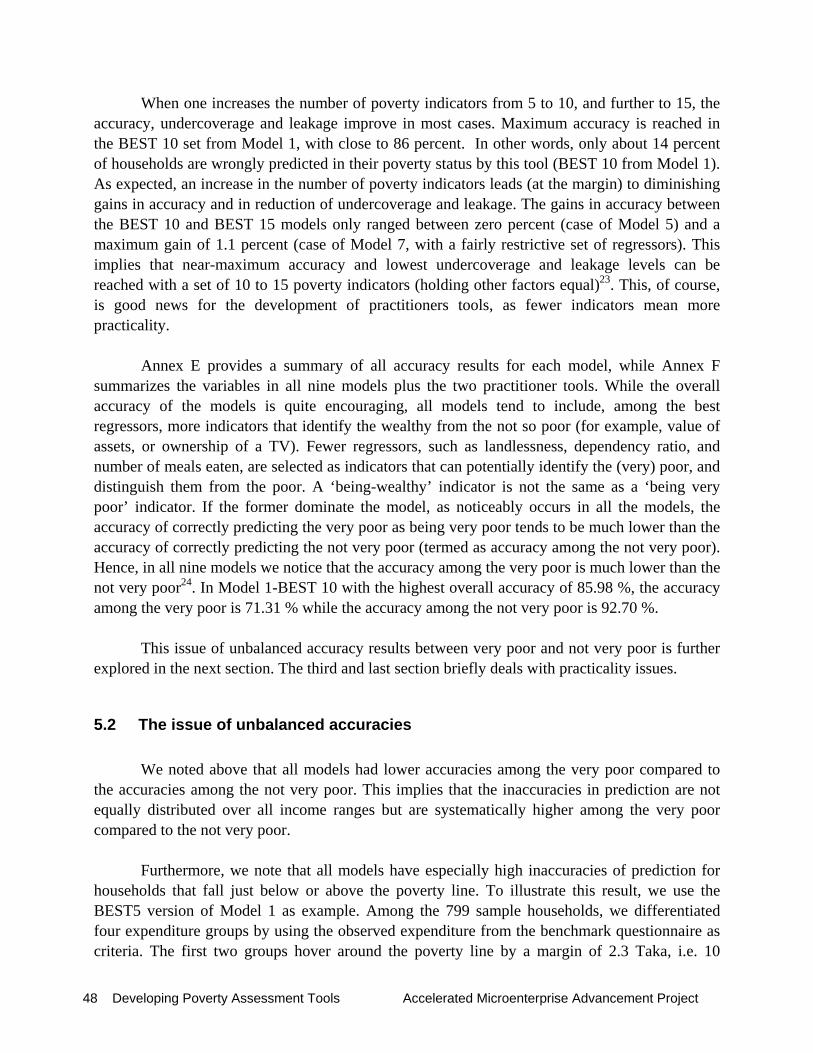
48 Developing Poverty Assessment Tools Accelerated Microenterprise Advancement Project
When one increases the number of poverty indicators from 5 to 10, and further to 15, the accuracy, undercoverage and leakage improve in most cases. Maximum accuracy is reached in the BEST 10 set from Model 1, with close to 86 percent. In other words, only about 14 percent of households are wrongly predicted in their poverty status by this tool (BEST 10 from Model 1). As expected, an increase in the number of poverty indicators leads (at the margin) to diminishing gains in accuracy and in reduction of undercoverage and leakage. The gains in accuracy between the BEST 10 and BEST 15 models only ranged between zero percent (case of Model 5) and a maximum gain of 1.1 percent (case of Model 7, with a fairly restrictive set of regressors). This implies that near-maximum accuracy and lowest undercoverage and leakage levels can be reached with a set of 10 to 15 poverty indicators (holding other factors equal)23. This, of course, is good news for the development of practitioners tools, as fewer indicators mean more practicality.
Annex E provides a summary of all accuracy results for each model, while Annex F
summarizes the variables in all nine models plus the two practitioner tools. While the overall accuracy of the models is quite encouraging, all models tend to include, among the best regressors, more indicators that identify the wealthy from the not so poor (for example, value of assets, or ownership of a TV). Fewer regressors, such as landlessness, dependency ratio, and number of meals eaten, are selected as indicators that can potentially identify the (very) poor, and distinguish them from the poor. A ‘being-wealthy’ indicator is not the same as a ‘being very poor’ indicator. If the former dominate the model, as noticeably occurs in all the models, the accuracy of correctly predicting the very poor as being very poor tends to be much lower than the accuracy of correctly predicting the not very poor (termed as accuracy among the not very poor). Hence, in all nine models we notice that the accuracy among the very poor is much lower than the not very poor24. In Model 1-BEST 10 with the highest overall accuracy of 85.98 %, the accuracy among the very poor is 71.31 % while the accuracy among the not very poor is 92.70 %.
This issue of unbalanced accuracy results between very poor and not very poor is further explored in the next section. The third and last section briefly deals with practicality issues.
5.2 The issue of unbalanced accuracies
We noted above that all models had lower accuracies among the very poor compared to the accuracies among the not very poor. This implies that the inaccuracies in prediction are not equally distributed over all income ranges but are systematically higher among the very poor compared to the not very poor.
Furthermore, we note that all models have especially high inaccuracies of prediction for households that fall just below or above the poverty line. To illustrate this result, we use the BEST5 version of Model 1 as example. Among the 799 sample households, we differentiated four expenditure groups by using the observed expenditure from the benchmark questionnaire as criteria. The first two groups hover around the poverty line by a margin of 2.3 Taka, i.e. 10
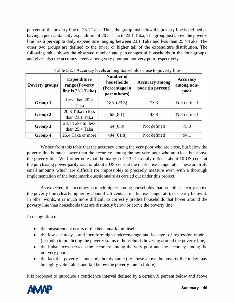
Summary 49
percent of the poverty line of 23.1 Taka. Thus, the group just below the poverty line is defined as having a per-capita daily expenditure of 20.8 Taka to 23.1 Taka, The group just above the poverty line has a per-capita daily expenditure ranging between 23.1 Taka and less than 25.4 Taka. The other two groups are defined to the lower or higher tail of the expenditure distribution. The following table shows the observed number and percentages of households in the four groups, and gives also the accuracy levels among very poor and not very poor respectively.
Table 5.2.1 Accuracy levels among households close to poverty line
Poverty groups Expenditure
range (Poverty line is 23.1 Taka)
Number of households
(Percentage in parentheses)
Accuracy among poor (in percent)
Accuracy among non-
poor
Group 1 Less than 20.8 Taka 186 (23.3) 73.3 Not defined
Group 2 20.8 Taka to less than 23.1 Taka 65 (8.1) 43.8 Not defined
Group 3 23.1 Taka to less than 25.4 Taka 54 (6.8) Not defined 75.0
Group 4 25.4 Taka or more 494 (61.8) Not defined 94.1
We see from this table that the accuracy among the very poor who are close, but below the poverty line is much lower than the accuracy among the not very poor who are close but above the poverty line. We further note that the margin of 2.3 Taka only reflects about 10 US-cents at the purchasing power parity rate, or about 3 US-cents at the market exchange rate. These are truly small amounts which are difficult (or impossible) to precisely measure even with a thorough implementation of the benchmark questionnaire as carried out under this project.
As expected, the accuracy is much higher among households that are either clearly above the poverty line (clearly higher by about 3 US-cents at market exchange rate), or clearly below it. In other words, it is much more difficult to correctly predict households that hover around the poverty line than households that are distinctly below or above the poverty line. In recognition of
• the measurement errors of the benchmark tool itself • the low accuracy – and therefore high undercoverage and leakage- of regression models
(or tools) in predicting the poverty status of households hovering around the poverty line, • the imbalances between the accuracy among the very poor and the accuracy among the
not very poor • the fact that poverty is not static but dynamic (i.e. those above the poverty line today may
be highly vulnerable, and fall below the poverty line in future),
it is proposed to introduce a confidence interval defined by a certain X percent below and above

50 Developing Poverty Assessment Tools Accelerated Microenterprise Advancement Project
the poverty line that gives the benefit of the doubt to those being predicted as fairly close to the poverty line.

Summary 51
5.3 Practicality issues
As this report was concerned with accuracy tests, practicality issues were only briefly referred to when discussing our (admittedly subjective) choice in how to gradually restrict the set of regressors from Model 1 to Model 6. Two criteria guided us in the choice of which variables to exclude from one model to the next: the difficulty (costs and time) in obtaining (valid and reliable) information on indicators; and the degree of verifiability of indicators (again, counting costs and time) so as to reduce the possibility for strategic answers or actions to alter one’s poverty status or outreach. Using these criteria, models 1 thru 6 were differentiated by successively excluding indicators with low practicality. In Model 7, an effort was made to include only those poverty indicators that were rated by the experienced management staff of DATA in Bangladesh as highly verifiable (i.e. receiving a score of five on a range from one to five). The forthcoming practicality tests should provide an enhanced information basis on the practicality of different indicators, and it is recommended that practitioners participating in practicality tests also rate the indicators tested on a subjective scale from 1 to 5. These scales may be further differentiated into two subcriteria: difficulty of obtaining and of verifying the information.

52 Developing Poverty Assessment Tools Accelerated Microenterprise Advancement Project
Bibliography Bangladesh Bureau of Statistics (2002). Report the Poverty Monitoring Survey May 1999. Dhaka, Bangladesh. Bangladesh Bureau of Statistics (2003). Statistical Yearbook of Bangladesh, 22nd edition (December). Dhaka, Bangladesh. Gibbons David S., Anton Simanowitz, and Benjamin Nkuna. 1999. CASHPOR-SEF Operational Manual, Cost-effective Targeting: Two Tools to Identify the Poor. Edited by Helen Todd. Produced by CASHPOR Technical Services. Sermban, Negri Sembilan, Malaysia. Grootaert, Christiaan, and Jeanine Braithwaite. 1998. “Poverty correlates and indicator-based targeting in eastern Europe and the Former Soviet Union.” Poverty Reduction and Economic Management Network, Environmentally and Socially Sustainable Development Network. Washington D.C.: The World Bank. Henry, Carla, Manohar Sharma, Cécile Lapenu, and Manfred Zeller. 2003. Microfinance poverty assessment tool. Technical Tools Series No. 5, September 2003. Published by the Consultative Group to Assist the Poor (CGAP) and The World Bank, Washington, D.C. ISBN-0-8213-5674-7 (PDF-File at http://www.cgap.org/ ). Matin, Imran, Marie Jo Cortijo, and Zakir Hassan. 2003. An assessment of the poverty outreach of Palli Daridro Bimochon Foundation (PDBF). Report prepared for CIDA, Canada.
Schreiner, Mark. 2001. Seven aspects of loan size. Journal of Microfinance, Vol. 3, No. 2. Zeller, Manfred, Manohar Sharma, Akhter Ahmed, and Shahidur Rashid. 2002. Group-based financial institutions for the rural poor in Bangladesh: An institutional-and household-level analysis. Research report No. 120. Washington, D.C.: International Food Policy Research Institute. Zeller, Manfred, Manohar Sharma, Carla J. Henry, and Cécile Lapenu. 2001. An operational tool for evaluating poverty outreach of development policies and projects. Discussion Paper No. 111, Food Consumption and Nutrition Division, International Food Policy Research Institute, Washington, D.C, June). (PDF-File at http://www.ifpri.org/ ). Zeller, Manfred. 2004. Review of Poverty Assessment Tools. Report submitted to IRIS and USAID as part of the Developing Poverty Assessment Tools Project. (PDF-File at http://www.povertytools.org ). Zeller, Manfred et al. 2004. An evaluation of participatory wealth ranking as a poverty targeting and assessment tool for various geographic levels. Unpublished manuscript, Institute of Rural Development, University of Göttingen, Germany.

Annexes 53
Annexes
Annex A: Size and distribution of sample
Division District Thana Union Number of
survey households
Sample for Participatory
Wealth Ranking
Barisal Barguna Bamna Bamna 40 40
Barisal Barguna Bamna Dauatala 40 40
Chittagong Chandpur Hajiganj Uttar
Gandharabpur
40
Chittagong Chandpur Hajiganj Uttar Rajargaon 40
Chittagong Cox’s Bazar Chakaria Dulahazara 40
Chittagong Cox’s Bazar Chakaria Magnama 40
Dhaka Dhaka Nowabganj Agla 40
Dhaka Dhaka Nowabganj Joykrishnapur 40
Dhaka Madaripur Rajoir Isibpur 40 40
Dhaka Madaripur Rajoir Paikpara 40 40
Dhaka Netrokona Khaliajuri Khaliajuri 40
Dhaka Netrokona Khaliajuri Nagar 40
Khulna Jessore Jessore Arabpur 40
Khulna Jessore Jessore Lebutala 40
Rajshahi Bogra Gabtali Gabtali 40 40
Rajshahi Bogra Gabtali Nepaltali 40 40
Rajshahi Naogaon Porsha Ghatnagar 40
Rajshahi Naogaon Porsha Tentulia 40
Rajshahi Rangpur Pirganj Bara Alampur 40 40
Rajshahi Rangpur Pirganj Mithapur 40 40
Total 800 320

54 Developing Poverty Assessment Tools Accelerated Microenterprise Advancement Project
Annex B: Descriptives of all regressors (n= 253), by type of model
Variable label Min. Max. Mean S. Dev. M1 M2 M3 M4 M5 M6 M7 M8 M9 M10Age of household head 18 85 44.64 13.46 X X X X X X X X X X Household size 1 24 4.93 2.11 X X X X X X X X X X Household size squared 1 576 28.75 32.34 X X X X X X X X X X Division 1 0 1 0.30 0.46 X X X X X X X X X X Division 2 0 1 0.20 0.40 X X X X X X X X X X Division 3 0 1 0.10 0.30 X X X X X X X X X X Division 4 0 1 0.30 0.46 X X X X X X X X X X Education level spouse 0 14 0.00 X X X X X X X Household owns any of motor tiller, wooden plow, tube irrigation or husking machine 0 4 0.32 0.69 X X X X X X X X X
Average age of all household members 8.6 77.5 26.07 10.11 X X X X X X X Squared age of household head 324 7225 2173.88 1301.88 X X X X X X X X Part A, subjective ranking scale 1 to 5 compared to community 1 5 2.45 0.96 X X X X X
Average of household members, except head 1 65 15.86 7.47 X X X X X X X
Head of household is beggar (1=Yes, 0=no) 0 1 0.00 0.05 X X X X X X X X X X Blanket ownership 0 1 0.72 0.45 X X X X X X X X X Boat ownership 0 1 0.08 0.27 X X X X X X X X X Household has borrowed in past 3 years for emergencies 0 1 0.39 0.49 X X X X
Household has borrowed in past 3 years from informal market 0 1 0.53 0.50 X X X X
Dummy household borrows from informal market 0 1 0.68 0.47 X X X X
Black and white TV ownership 0 1 0.13 0.34 X X X X X X X X X The percentage of amount you would spend on food if you were given an additional 100 Taka tomorrow?
0 100 58.71 31.38 X X X X
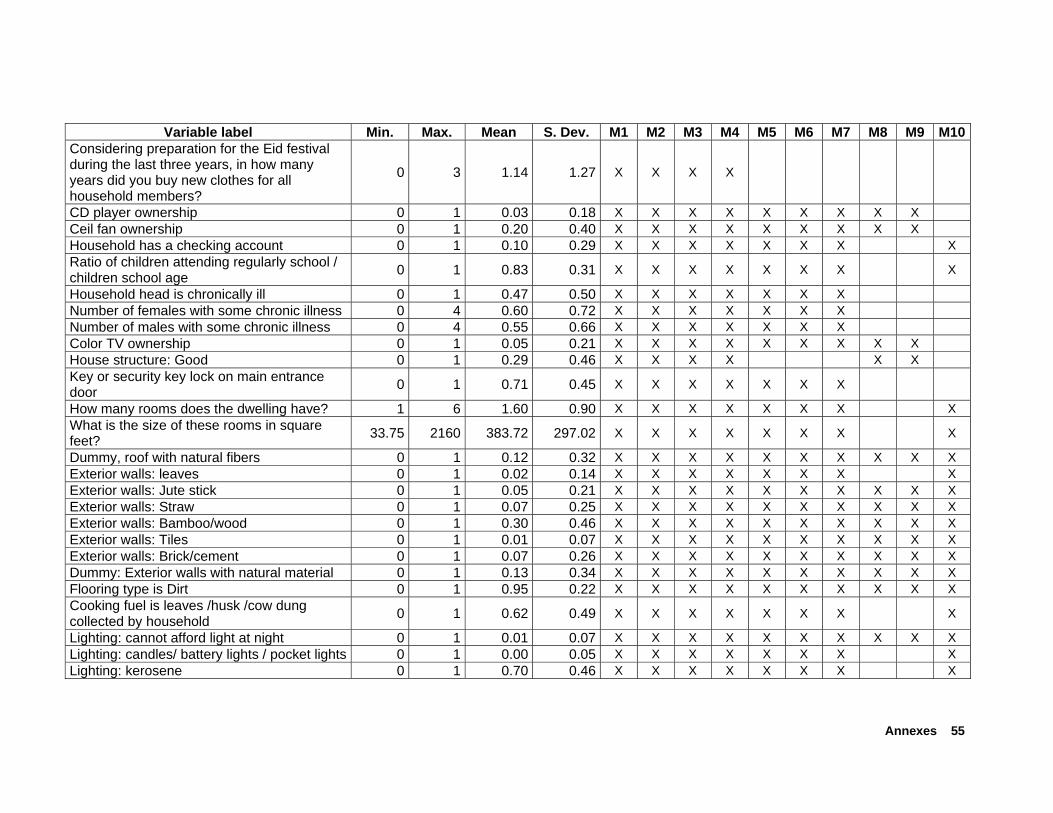
Annexes 55
Variable label Min. Max. Mean S. Dev. M1 M2 M3 M4 M5 M6 M7 M8 M9 M10Considering preparation for the Eid festival during the last three years, in how many years did you buy new clothes for all household members?
0 3 1.14 1.27 X X X X
CD player ownership 0 1 0.03 0.18 X X X X X X X X X Ceil fan ownership 0 1 0.20 0.40 X X X X X X X X X Household has a checking account 0 1 0.10 0.29 X X X X X X X X Ratio of children attending regularly school / children school age 0 1 0.83 0.31 X X X X X X X X
Household head is chronically ill 0 1 0.47 0.50 X X X X X X X Number of females with some chronic illness 0 4 0.60 0.72 X X X X X X X Number of males with some chronic illness 0 4 0.55 0.66 X X X X X X X Color TV ownership 0 1 0.05 0.21 X X X X X X X X X House structure: Good 0 1 0.29 0.46 X X X X X X Key or security key lock on main entrance door 0 1 0.71 0.45 X X X X X X X
How many rooms does the dwelling have? 1 6 1.60 0.90 X X X X X X X X What is the size of these rooms in square feet? 33.75 2160 383.72 297.02 X X X X X X X X
Dummy, roof with natural fibers 0 1 0.12 0.32 X X X X X X X X X X Exterior walls: leaves 0 1 0.02 0.14 X X X X X X X X Exterior walls: Jute stick 0 1 0.05 0.21 X X X X X X X X X X Exterior walls: Straw 0 1 0.07 0.25 X X X X X X X X X X Exterior walls: Bamboo/wood 0 1 0.30 0.46 X X X X X X X X X X Exterior walls: Tiles 0 1 0.01 0.07 X X X X X X X X X X Exterior walls: Brick/cement 0 1 0.07 0.26 X X X X X X X X X X Dummy: Exterior walls with natural material 0 1 0.13 0.34 X X X X X X X X X X Flooring type is Dirt 0 1 0.95 0.22 X X X X X X X X X X Cooking fuel is leaves /husk /cow dung collected by household 0 1 0.62 0.49 X X X X X X X X
Lighting: cannot afford light at night 0 1 0.01 0.07 X X X X X X X X X X Lighting: candles/ battery lights / pocket lights 0 1 0.00 0.05 X X X X X X X X Lighting: kerosene 0 1 0.70 0.46 X X X X X X X X

56 Developing Poverty Assessment Tools Accelerated Microenterprise Advancement Project
Variable label Min. Max. Mean S. Dev. M1 M2 M3 M4 M5 M6 M7 M8 M9 M10Lighting: gas lamp 0 1 0..00 0..04 X X X X X X X X X X Lighting: tap electricity socket of neighbor / public grid 0 1 0..02 0..14 X X X X X X X X
Lighting: Public grid / legal socket in house 0 1 0.27 0.44 X X X X X X X X X X Lighting: own private generator 0 1 0.00 0.04 X X X X X X X X X X Dummy: Own Well/borehole sealed in residence yard 0 1 0.01 0.08 X X X X X X X X X X
Toilet: bush, field, no facility 0 1 0.24 0.43 X X X X X X X X X X Toilet: shared pit toilet 0 1 0.13 0.33 X X X X X X X X Toilet: own pit toilet 0 1 0.38 0.49 X X X X X X X X Toilet: shared, ventilated improved latrine 0 1 0.04 0.20 X X X X X X X X Toilet: own, ventilated improved latrine 0 1 0.21 0.41 X X X X X X X X Household has improved toilet 0 1 0.25 0.43 X X X X X X X X X X Household shares toilet 0 1 0.17 0.37 X X X X X X X X X X Dummy: Head of household sleeps on a bed 0 1 0.73 0.45 X X X X X X X X X Dummy: household cooks in separate kitchen 0 1 0.59 0.49 X X X X X X X X X X
Do you have Telephone (fixed land line) in the house? 0 1 0.01 0.09 X X X X X X X X X X
Do you have Mobile (cell phone) in the house? 0 1 0.02 0.12 X X X X X X X X X X
Male accepts wage at pov line ? 1 = yes 0 1 0.44 0.50 X X X X Female accepts wage at pov line ? 1 = yes 0 1 0.20 0.40 X X X X Head of household is agr or non agr daily worker (1=Yes, 0=no) 0 1 0.24 0.43 X X X X X X X X
Head of household is agricultural daily worker (1=Yes, 0=no) 0 1 0.15 0.36 X X X X X X X X
Head of household is nonagricultural daily worker (1=Yes, 0=no) 0 1 0.10 0.30 X X X X X X X X
% of household members with any disability (in relation to household size) 0 50 1.29 5.63 X X X X X X X X
Household head has any disability 0 1 0.02 0.12 X X X X X X X X X Household head is divorced 0 1 0.00 0.06 X X X X X X X X X X
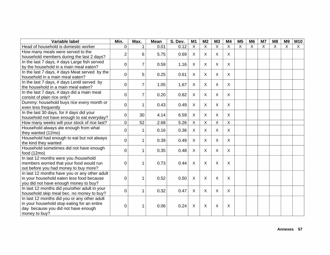
Annexes 57
Variable label Min. Max. Mean S. Dev. M1 M2 M3 M4 M5 M6 M7 M8 M9 M10Head of household is domestic worker 0 1 0.01 0.12 X X X X X X X X X X How many meals were served to the household members during the last 2 days? 2 6 5.75 0.69 X X X X
In the last 7 days, # days Large fish served by the household in a main meal eaten? 0 7 0.59 1.16 X X X X
In the last 7 days, # days Meat served by the household in a main meal eaten? 0 5 0.25 0.61 X X X X
In the last 7 days, # days Lentil served by the household in a main meal eaten? 0 7 1.05 1.67 X X X X
In the last 7 days, # days did a main meal consist of plain rice only? 0 7 0.20 0.82 X X X X
Dummy: household buys rice every month or even less frequently 0 1 0.43 0.49 X X X X
In the last 30 days, for # days did your household not have enough to eat everyday? 0 30 4.14 6.59 X X X X
How many weeks will your stock of rice last? 0 52 2.68 5.26 X X X X Household always ate enough from what they wanted (12mo) 0 1 0.16 0.36 X X X X
Household had enough to eat but not always the kind they wanted 0 1 0.39 0.49 X X X X
Household sometimes did not have enough food (12mo) 0 1 0.35 0.48 X X X X
In last 12 months were you /household members worried that your food would run out before you had money to buy more?
0 1 0.73 0.44 X X X X
In last 12 months have you or any other adult in your household eaten less food because you did not have enough money to buy?
0 1 0.52 0.50 X X X X
In last 12 months did you/other adult in your household skip meal bec. no money to buy? 0 1 0.32 0.47 X X X X
In last 12 months did you or any other adult in your household stop eating for an entire day because you did not have enough money to buy?
0 1 0.06 0.24 X X X X

58 Developing Poverty Assessment Tools Accelerated Microenterprise Advancement Project
Variable label Min. Max. Mean S. Dev. M1 M2 M3 M4 M5 M6 M7 M8 M9 M10Household ate less food e13 more than 30 days during past 12 months 0 1 0.22 0.41 X X X X
Household had to skip meals last 12 months 0 1 0.32 0.47 X X X X Household never eats rice starch 0 1 0.87 0.34 X X X X Household never eats broken rice 0 1 0.76 0.42 X X X X Education level of household head (median) 0 16 0.00 X X X X X X X X Education level of household members excluding household head (median) 0 12 1.00 X X X X X X X X
Household has electricity 0 1 0.28 0.45 X X X X X X X X X X Homestead area (decimal) 0 120 8.29 9.81 X X X X X X X X Agri. Land (under irrigation) area (decimal) 0 1920 56.38 165.02 X X X X X X X X Agri. Land (under no irrigation) area (dec) 0.00 1920.0 18.53 92.46 X X X X X X X X Head of household is farmer (1=Yes, 0=no) 0 1 0.28 0.45 X X X X X X X X X X Households % have access to FFE 6 48 18.72 15.30 X X X X X X X Household did not eat for entire days in past 12 mo. 0 1 0.06 0.24 X X X X
Food exp share, C, in % 0.19 1.83 1.32 0.30 X X X X I feel accepted as a member of this village 0 1 0.88 0.33 X X X X If you lose a goat or sheep, someone in village will help to look for it or return it 0 1 0.82 0.38 X X X X
Household in political group 0 1 0.04 0.20 X X X X X X X Household in school committee 0 1 0.03 0.17 X X X X X X X Household in youth group 0 1 0.02 0.14 X X X X X X X Have you or members of household are denied service or only limited opportunity to health services/clinics
0 1 0.03 0.16 X X X X
Have you or members of household are denied service or only limited opportunity to credit/finance
0 1 0.04 0.19 X X X X
Have you or members of household are denied service or only limited opportunity to security/police services
0 1 0.02 0.13 X X X X
Ratio girls to boys in school attendance 0 3 0.95 0.35 X X X X X X X
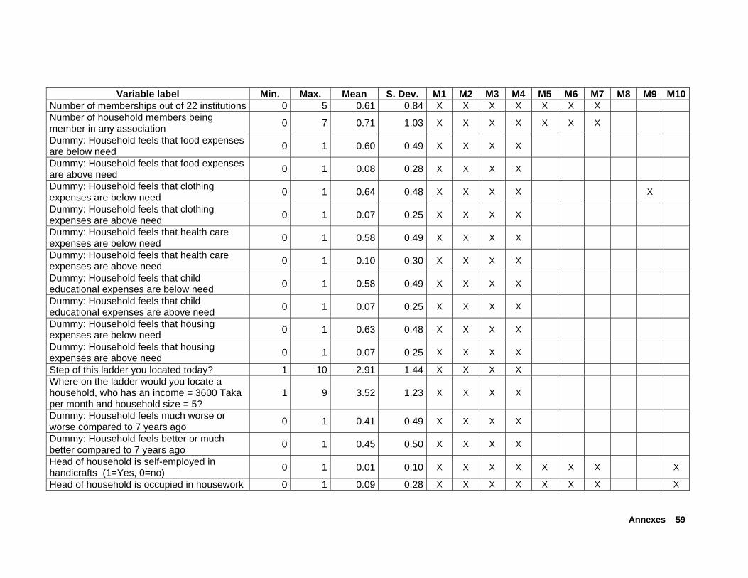
Annexes 59
Variable label Min. Max. Mean S. Dev. M1 M2 M3 M4 M5 M6 M7 M8 M9 M10Number of memberships out of 22 institutions 0 5 0.61 0.84 X X X X X X X Number of household members being member in any association 0 7 0.71 1.03 X X X X X X X
Dummy: Household feels that food expenses are below need 0 1 0.60 0.49 X X X X
Dummy: Household feels that food expenses are above need 0 1 0.08 0.28 X X X X
Dummy: Household feels that clothing expenses are below need 0 1 0.64 0.48 X X X X X
Dummy: Household feels that clothing expenses are above need 0 1 0.07 0.25 X X X X
Dummy: Household feels that health care expenses are below need 0 1 0.58 0.49 X X X X
Dummy: Household feels that health care expenses are above need 0 1 0.10 0.30 X X X X
Dummy: Household feels that child educational expenses are below need 0 1 0.58 0.49 X X X X
Dummy: Household feels that child educational expenses are above need 0 1 0.07 0.25 X X X X
Dummy: Household feels that housing expenses are below need 0 1 0.63 0.48 X X X X
Dummy: Household feels that housing expenses are above need 0 1 0.07 0.25 X X X X
Step of this ladder you located today? 1 10 2.91 1.44 X X X X Where on the ladder would you locate a household, who has an income = 3600 Taka per month and household size = 5?
1 9 3.52 1.23 X X X X
Dummy: Household feels much worse or worse compared to 7 years ago 0 1 0.41 0.49 X X X X
Dummy: Household feels better or much better compared to 7 years ago 0 1 0.45 0.50 X X X X
Head of household is self-employed in handicrafts (1=Yes, 0=no) 0 1 0.01 0.10 X X X X X X X X
Head of household is occupied in housework 0 1 0.09 0.28 X X X X X X X X

60 Developing Poverty Assessment Tools Accelerated Microenterprise Advancement Project
Variable label Min. Max. Mean S. Dev. M1 M2 M3 M4 M5 M6 M7 M8 M9 M10Manual husking machine 0 1 0.10 0.30 X X X X X X X X X Do you or your partner/spouse or anyone else in your household have a withdrawable savings account?
0 1 0.29 0.45 X X X X X X X
Dummy, if household rates itself below the step reflecting the poverty line 0 1 0.62 0.49 X X X X
Household owns less than 50 decimals of land, including homestead 0 1 0.67 0.47 X X X X X X X X X
Ln, value ceil fan 0 8.29 1.38 2.76 X X X X X Ln average cloth. exp. per capita, past 12 mo 0.76 8.13 6.19 0.97 X X X X X Ln, value color tv 0 10.74 0.45 2.00 X X X X X X X Head of household chooses leisure 0 1 0.04 0.18 X X X X X X X X X X Ln, value of radio, TV, VCR and cd player 0.00 10.78 2.39 3.48 X X X X X X X Ln, value of electric - gas cooker 0 9.47 0.03 0.47 X X X X X X X Household lends money to other households 0 1 0.17 0.37 X X X X Ln, value of agricultural land under irrigation 4.60 14.42 7.50 3.61 X X X X X X Ln, value of agricultural land no irrigation 3.21 14.22 4.72 3.15 X X X X X X Ln, annualized food expenditures recall average week 8.20 12.37 10.27 0.49 X
% of adult household members read & write 0 100.00 24.64 25.33 X X X X X X X Household head can read and write 0 1 0.39 0.49 X X X X X X X X Ln, money received from family members working elsewhere 3.00 12.61 4.48 2.85 X X X X X X X X
Ln, value bike 0 8.52 1.54 2.81 X X X X X X X Ln, Household food expenditures per week 3.22 7.82 5.98 0.56 X Ln, value food produced by household in farm / garden / gathers / consumes, per week 0 7.78 4.24 1.74 X
Ln, household monthly expenditure on utilities (electricity, phone, water, etc) 0 7.82 1.61 2.23 X X X
Ln, household monthly exp. on transport 0 8.16 3.95 1.76 X Ln, household monthly expenditure on fuel 0 6.91 3.81 1.33 X Ln, value of other goods prod. by household in garden and then consumes, month 0 8.52 4.78 1.33 X

Annexes 61
Variable label Min. Max. Mean S. Dev. M1 M2 M3 M4 M5 M6 M7 M8 M9 M10Ln, household expenditure on school/education in last 12 months 0 10.31 4.61 3.48 X
Ln, household expend. health in last 12 mo. 0 11.51 7.40 1.29 X Ln, household expend. home in last 12 mo. 0 12.74 5.00 3.74 X Ln, household expenditure on furniture/appliances in last 12 months 0.00 11.29 2.83 3.16 X
Ln, remittances sent by household to other relatives in last 12 months 0.00 11.16 0.81 2.45 X X
Ln, household expend. on other expenditures in last 12 mo (soc events, gifts, taxes) 0.00 11.53 4.60 3.37 X
Ln, average clothing expenditures females 0.00 8.25 6.20 1.22 X Ln, average clothing expenditures males 0.00 8.23 6.07 1.20 X Ln, value milk cows -0.69 11.41 2.91 3.54 X X X X X X X Ln, estimated sale value of house 4.41 14.32 10.16 2.11 X X X X X X X Ln, costs of recent home improvements 2.34 12.90 6.96 2.79 X X X X X Ln, min wage male income earner accept for 8 hs work peak season 3.69 5.52 4.62 0.21 X X X X
Ln, min wage female income earner accept for 8 hs work peak season 3.40 5.01 4.36 0.12 X X X X
Ln, value of homestead including land plot 4.05 14.22 9.72 1.97 X X X X X X X X X Ln, value of dowry given by household 0.03 10.82 0.72 2.41 X X X X X Ln, value of dowry received by household 1.42 12.61 2.48 2.82 X X X X X Ln, how much does your household need per month to live? 6.91 9.74 8.31 0.46 X X X X
Ln, value of jewelry owned by household 1.53 12.61 6.00 2.73 X X X X X X Ln, value of biggest loan for food/emergency 1.31 11.51 4.07 3.52 X X X X X Ln, value of informal debt owed by household 1.77 12.35 5.16 3.41 X X X X X Ln, value of debt owed by other household to household 1.18 13.02 2.40 2.82 X X X X X
Ln, amount of outstanding/most recent loan disbursed (only 2003-2004) 0 12.68 2.07 3.81 X X X X X X
Ln, value of other land 3.27 14.69 6.20 3.42 X X X X X X Ln, value radio 0.00 8.16 1.35 2.52 X X X X X

62 Developing Poverty Assessment Tools Accelerated Microenterprise Advancement Project
Variable label Min. Max. Mean S. Dev. M1 M2 M3 M4 M5 M6 M7 M8 M9 M10Ln, value of savings husband 1.10 12.61 2.32 2.81 X X X X X Ln, value of formal savings spouse -0.18 11.58 0.63 2.51 X X X X X Ln, value of household total savings 1.58 12.63 3.46 3.19 X X X X X X Ln annual tot. summary of expend. section C 8.83 12.89 10.68 0.58 X Ln total value of household assets 4.94 13.32 8.75 1.38 X X Ln, value of transportation assets 0 13.27 2.72 3.57 X X X X X Number of days in past 7 days any of four superior food eaten 0 21 3.15 3.74 X X X X X
Household head is married and spouse is permanently in household 0 1 0.89 0.31 X X X X X X X X X X
Mosquito net ownership 0 1 0.94 0.24 X X X X X X X X X Motorcycle ownership 0 1 0.01 0.09 X X X X X X X X X Motor tiller ownership 0 1 0.02 0.14 X X X X X X X X X Maximal education level females (median) 0 16 4.00 X X X X X X X Maximal education level males (median) 0 16 4.00 X X X X X X X Number of auto rickshaws owned household 0 1 0.00 0.04 X X X X X X X X Number of beds owned by household 0 11 1.77 1.43 X X X X X X X X X X Number of bicycles owned by household 0 2 0.25 0.47 X X X X X X X X X X Number of blankets owned by household 0 15 1.85 1.92 X X X X X X X X X X Number of boats owned by household 0 3 0.08 0.29 X X X X X X X X X X Number of black and white TV owned 0 1 0.13 0.34 X X X X X X X X X X Cattle number 0 8 0.53 1.08 X X X X X X X X X X Number of cd players owned by household 0 1 0.03 0.18 X X X X X X X X Number of ceil fans owned by household 0 5 0.37 0.85 X X X X X X X X X X Number of color TVs owned by household 0 2 0.05 0.22 X X X X X X X X X X Is the minimum monthly income H06 below objective poverty line 1=Yes 0 1 0.26 0.44 X X X X
Number of electronic or gas cookers owned 0 1 0.00 0.06 X X X X X X X X X X Number of husk machines owned by household 0 1 0.10 0.30 X X X X X X X X X X
Number of kantha owned by household 0 30 6.75 4.59 X X X X X X X X X X Number of metal cooking pots owned by household 0 65 10.08 7.61 X X X X X X X X X X
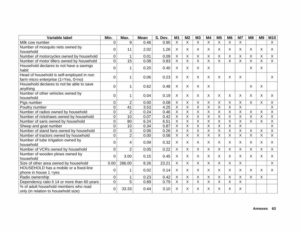
Annexes 63
Variable label Min. Max. Mean S. Dev. M1 M2 M3 M4 M5 M6 M7 M8 M9 M10Milk cow number 0 9 0.46 0.95 X X X X X X X X Number of mosquito nets owned by household 0 11 2.02 1.26 X X X X X X X X X X
Number of motorcycles owned by household 0 1 0.01 0.09 X X X X X X X X X X Number of motor tillers owned by household 0 15 0.08 0.83 X X X X X X X X X X Household declares to not have a savings habit 0 1 0.20 0.40 X X X X X X
Head of household is self-employed in non farm micro enterprise (1=Yes, 0=no) 0 1 0.06 0.23 X X X X X X X X
Household declares to not be able to save anything 0 1 0.62 0.48 X X X X X X
Number of other vehicles owned by household 0 1 0.04 0.19 X X X X X X X X X X
Pigs number 0 2 0.00 0.08 X X X X X X X X X X Poultry number 0 41 3.53 4.25 X X X X X X X X Number of radios owned by household 0 2 0.24 0.46 X X X X X X X X X X Number of rickshaws owned by household 0 10 0.07 0.42 X X X X X X X X X X Number of saris owned by household 0 80 6.24 6.51 X X X X X X X X X X Sheep and goat number 0 10 0.34 0.87 X X X X X X X X Number of stand fans owned by household 0 3 0.06 0.26 X X X X X X X X X X Number of tractors owned by household 0 2 0.00 0.08 X X X X X X X X X X Number of tube irrigation owned by household 0 4 0.09 0.32 X X X X X X X X X X
Number of VCRs owned by household 0 2 0.05 0.22 X X X X X X X X X X Number of wooden plows owned by household 0 3.00 0.15 0.45 X X X X X X X X X X
Size of other area owned by household 0.00 286.00 8.26 23.21 X X X X X X X X HOUSEHOLD has a mobile or a fixed-line phone in house 1 =yes 0 1 0.02 0.14 X X X X X X X X X X
Radio ownership 0 1 0.23 0.42 X X X X X X X X X Dependency ratio lt 14 or more than 60 years 0 5 0.89 0.79 X X X X X X X % of adult household members who read only (in relation to household size) 0 33.33 0.44 3.10 X X X X X X X
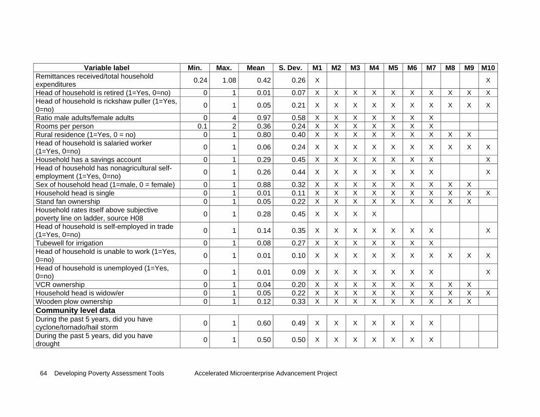
64 Developing Poverty Assessment Tools Accelerated Microenterprise Advancement Project
Variable label Min. Max. Mean S. Dev. M1 M2 M3 M4 M5 M6 M7 M8 M9 M10Remittances received/total household expenditures 0.24 1.08 0.42 0.26 X X
Head of household is retired (1=Yes, 0=no) 0 1 0.01 0.07 X X X X X X X X X X Head of household is rickshaw puller (1=Yes, 0=no) 0 1 0.05 0.21 X X X X X X X X X X
Ratio male adults/female adults 0 4 0.97 0.58 X X X X X X X Rooms per person 0.1 2 0.36 0.24 X X X X X X X Rural residence (1=Yes, 0 = no) 0 1 0.80 0.40 X X X X X X X X X Head of household is salaried worker (1=Yes, 0=no) 0 1 0.06 0.24 X X X X X X X X X X
Household has a savings account 0 1 0.29 0.45 X X X X X X X X Head of household has nonagricultural self-employment (1=Yes, 0=no) 0 1 0.26 0.44 X X X X X X X X
Sex of household head (1=male, 0 = female) 0 1 0.88 0.32 X X X X X X X X X Household head is single 0 1 0.01 0.11 X X X X X X X X X X Stand fan ownership 0 1 0.05 0.22 X X X X X X X X X Household rates itself above subjective poverty line on ladder, source H08 0 1 0.28 0.45 X X X X
Head of household is self-employed in trade (1=Yes, 0=no) 0 1 0.14 0.35 X X X X X X X X
Tubewell for irrigation 0 1 0.08 0.27 X X X X X X X Head of household is unable to work (1=Yes, 0=no) 0 1 0.01 0.10 X X X X X X X X X X
Head of household is unemployed (1=Yes, 0=no) 0 1 0.01 0.09 X X X X X X X X
VCR ownership 0 1 0.04 0.20 X X X X X X X X X Household head is widow/er 0 1 0.05 0.22 X X X X X X X X X X Wooden plow ownership 0 1 0.12 0.33 X X X X X X X X X Community level data During the past 5 years, did you have cyclone/tornado/hail storm 0 1 0.60 0.49 X X X X X X X
During the past 5 years, did you have drought 0 1 0.50 0.50 X X X X X X X
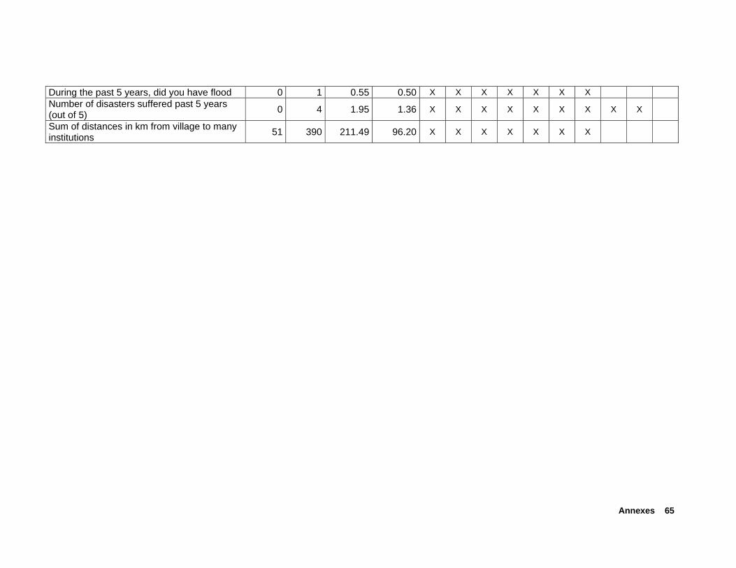
Annexes 65
During the past 5 years, did you have flood 0 1 0.55 0.50 X X X X X X X Number of disasters suffered past 5 years (out of 5) 0 4 1.95 1.36 X X X X X X X X X
Sum of distances in km from village to many institutions 51 390 211.49 96.20 X X X X X X X

66 Developing Poverty Assessment Tools Accelerated Microenterprise Advancement Project
Annex C: Gender-specific variables used in regression analysis
Variable Min. Max. Mean Std. Dev. Sex of household head 0 1 0.88 0.322 Maximal education level females (median) 0 16 4
Maximal education level males (median) 0 16 4
Number of females with some chronic illness 0.00 4.00 0.5982 0.72378
Number of males with some chronic illness 0.00 4.00 0.5532 0.66178
Ratio girls to boys in school attendance 0.00 3.00 0.9521 0.34581
Male accepts wage at pov line ? 1 = yes 0 1 0.44 0.497
Female accepts wage at pov line ? 1 = yes 0 1 0.20 0.400
Ln, Min wage male income earner accept for 8 hs hard work peak income season
3.69 5.52 5.0401 0.50367
Ln, Min wage female income earner accept for 8 hs hard work peak income season
3.40 5.30 5.1088 0.40157
Ln value of savings husband 0.00 12.61 1.4094 3.21053 Value of formal savings of spouse, log(Taka) 0.00 11.58 0.7980 2.45481
Education level spouse (median) 0 14 0
Ratio male adults/female adults 0.00 4.00 0.9703 0.58022 Ln, average clothing expenditures females 0.00 8.25 6.2021 1.22423
Ln, average clothing expenditures males 0.00 8.23 6.0741 1.20331
Number of saris owned by household 0.00 80 6.24 6.50
N = 799 Note: This list does not include gender-specific poverty indicators among the first set of about 700 regressors that were eliminated in preceding correlation and step-wise regression analysis because of insufficient correlation with per-capita daily expenditures.

Annexes 67
Annex D: Verifiability scores provided by survey firm DATA in Bangladesh Variable assessment scale: 1 very hard to verify– 5 easily verifiable
Variable label Verifiability score Education level spouse - adjusted 4 Household owns any of motor tiller, wooden plow, tube irrigation or husking machine 5
Average age of all household members 4 Average of household members, except head 4 Bed ownership 5 Head of household is beggar (1=Yes, 0=no) 5 Blanket ownership 5 Boat ownership 5 Household has borrowed in past 3 years for emergencies 3 Household has borrowed in past 3 years from informal market 3 Dummy household borrows from informal market and/or emergencies 3
Black and white TV ownership 5 CD player ownership 5 Ceil fan ownership 5 Household has a checking account 4 Ratio of children attending regularly school / children school age 4
Household head is chronically ill 3 Number of females with some chronic illness 3 Number of males with some chronic illness 3 Color TV ownership 5 During the past 5 years, did you have cyclone/tornado/hail storm 3
House structure: Good 5 Key or security key lock on main entrance door 1 How many rooms does the dwelling have? 4 Dummy, roof with natural fibers 5 Exterior walls: Jute stick 5 Exterior walls: Straw 5 Exterior walls: Bamboo/wood 5 Exterior walls: Tiles 5 Exterior walls: Brick/cement 5 Dummy: Exterior walls with natural material 5 Flooring type is Dirt 5 Lighting: cannot afford light at night 5 Lighting: candles/ battery lights / pocket lights 4 Lighting: kerosene 4 Lighting: gas lamp 5 Lighting: tap electricity socket of neighbor / public grid 3

68 Developing Poverty Assessment Tools Accelerated Microenterprise Advancement Project
Variable label Verifiability score
Lighting: Public grid with legal socket in house 5 Lighting: own private generator 5 Dummy: Own Well/borehole sealed in residence yard 5 Toilet: bush, field, no facility 5 Household has improved toilet 5 Household shares toilet 3 Dummy: Head of household sleeps on a bed 5 Dummy: household cooks in separate kitchen 5 Do you have Telephone (fixed land line) in the house? 5 Do you have Mobile (cell phone) in the house? 5 Male accepts wage at poverty line ? 1 = yes 3 Female accepts wage at poverty line ? 1 = yes 3 Head of household is agr or non agr daily worker (1=Yes, 0=no) 4
Head of household is agricultural daily worker (1=Yes, 0=no) 4 Head of household is nonagricultural daily worker (1=Yes, 0=no) 4
% of household members with any disability (in relation to household size) 4
Household head has any disability 5 Sum of distances in km from village to many institutions 3 Household head is divorced 5 Head of household is domestic worker (1=Yes, 0=no) 5 During the past 5 years, did you have drought 4 Education level of household head 4 Education level of household members excluding household head 3
Household has electricity 5 Homestead area (decimal) 4 Agricultural land (under irrigation) area (decimal) 3 Head of household is farmer (1=Yes, 0=no) 5 During the past 5 years, did you have flood 4 Household in political group 3 Household in school committee 4 Household in youth group 4 Ratio girls to boys in school attendance 3 Number of memberships out of 22 institutions 4 Number of household members being member in any association 3
Head of household is self-employed in handicrafts (1=Yes, 0=no) 4
Manual husking machine 5 Do you or your partner/spouse or anyone else in your household have a withdrawable savings account? 4
Dummy, if household rates itself below the step reflecting the pov line 3
Household own less than 50 decimals of land, including homestead 5

Annexes 69
Variable label Verifiability score Ln, value ceil fan 4 Ln average cloth. exp. per capita, past 12 mo 4 Ln, value color TV 5 Head of household chooses leisure (1=Yes, 0=no) 5 Ln, value of radio, TV, VCR and cd player 5 Ln, value of electric - gas cooker 5 Dummy household lends money to other households 4 Ln, value agr land under irrigation 3 Ln, value agr land under no irrigation 3 Ln, annualized food expenditures recall average week 3 % of adult household members who read and write 4 Household head can read and write 4 Ln of money received from family members working elsewhere 5
Ln, value bike 5 Ln, Household food expenditures per week 3 Ln, value food produced by household in farm or garden, or gathers and consumes, per week 3
Ln, household monthly expenditure on utilities (electricity, phone, water, etc) 5
Ln, household monthly expenditure on transport 3 Ln, household monthly expenditure on fuel 3 Ln, value of other goods produced by household in garden and then consumes, month 3
Ln, household expenditure on school/education in last 12 months 3
Ln, household expenditure on health in last 12 months 3 Ln, household expenditure on home in last 12 months 3 Ln, household expenditure on furniture/appliances in last 12 months 3
Ln, remittances sent by household to other relatives in last 12 months 3
Ln, household expenditure on other expenditures in last 12 mo (soc events, gifts, taxes) 3
Ln, milk cow resale value 5 Ln of estimated sales value of house 4 Ln of costs of recent home improvements 4 Ln, Min wage male income earner accept for 8 hs hard work peak income season 4
Ln, Min wage female income earner accept for 8 hs hard work peak income season 4
Ln value of homestead 5 Ln value of dowry received past 3 years 3 Ln value of dowry given past 3 years 3 Value of jewelry owned by household, log(Taka) 2 Ln, value of biggest loan for food/emergency 4 Informal debt owed by household, log(Taka) 3 Ln, value of debt owed by other households to household 3 Ln, amount of outstanding/most recent loan disbursed (03-04) 3
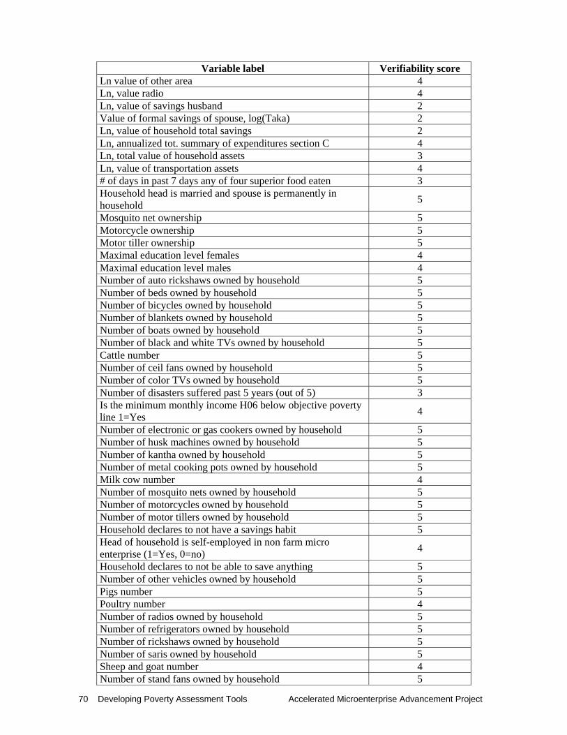
70 Developing Poverty Assessment Tools Accelerated Microenterprise Advancement Project
Variable label Verifiability score Ln value of other area 4 Ln, value radio 4 Ln, value of savings husband 2 Value of formal savings of spouse, log(Taka) 2 Ln, value of household total savings 2 Ln, annualized tot. summary of expenditures section C 4 Ln, total value of household assets 3 Ln, value of transportation assets 4 # of days in past 7 days any of four superior food eaten 3 Household head is married and spouse is permanently in household 5
Mosquito net ownership 5 Motorcycle ownership 5 Motor tiller ownership 5 Maximal education level females 4 Maximal education level males 4 Number of auto rickshaws owned by household 5 Number of beds owned by household 5 Number of bicycles owned by household 5 Number of blankets owned by household 5 Number of boats owned by household 5 Number of black and white TVs owned by household 5 Cattle number 5 Number of ceil fans owned by household 5 Number of color TVs owned by household 5 Number of disasters suffered past 5 years (out of 5) 3 Is the minimum monthly income H06 below objective poverty line 1=Yes 4
Number of electronic or gas cookers owned by household 5 Number of husk machines owned by household 5 Number of kantha owned by household 5 Number of metal cooking pots owned by household 5 Milk cow number 4 Number of mosquito nets owned by household 5 Number of motorcycles owned by household 5 Number of motor tillers owned by household 5 Household declares to not have a savings habit 5 Head of household is self-employed in non farm micro enterprise (1=Yes, 0=no) 4
Household declares to not be able to save anything 5 Number of other vehicles owned by household 5 Pigs number 5 Poultry number 4 Number of radios owned by household 5 Number of refrigerators owned by household 5 Number of rickshaws owned by household 5 Number of saris owned by household 5 Sheep and goat number 4 Number of stand fans owned by household 5

Annexes 71
Variable label Verifiability score Number of tractors owned by household 5 Number of tube irrigation owned by household 5 Number of VCRs owned by household 5 Number of wooden plows owned by household 5 Size of other area owned by household 4 Household has a mobile or a fixed-line phone in house 1 =yes 5 Radio ownership 5 Dependency ratio younger than 14 or more than 60 years old 4 % of adult household members who read only (in relation to household size) 4
Remittances received/total household expenditures 3 Head of household is retired (1=Yes, 0=no) 5 Head of household is rickshaw puller (1=Yes, 0=no) 5 Ratio male adults/female adults 4 Rooms per person 4 Does household live in rural area 5 Head of household is salaried worker (1=Yes, 0=no) 5 Household has a savings account 4 Head of household has nonagricultural self-employment (1=Yes, 0=no) 4
Sex of household head 5 Household head is single 5 Stand fan ownership 5 Head of household is self-employed in trade (1=Yes, 0=no) 4 Tubewell for irrigation ownership 4 Head of household is unable to work (1=Yes, 0=no) 5 Head of household is unemployed (1=Yes, 0=no) 4 VCR ownership 5 Household head is widow/er 5 Wooden plow ownership 5
Source: Communication via email in October 2004, scores given by DATA Ltd., Bangladesh
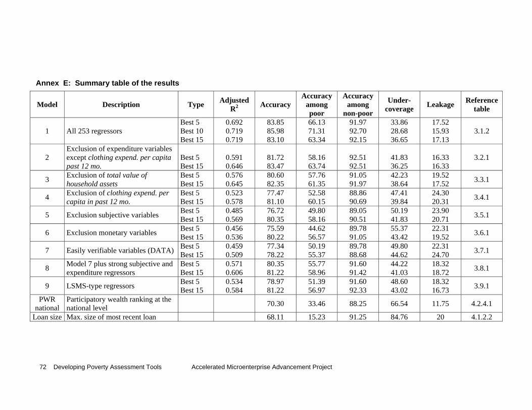
72 Developing Poverty Assessment Tools Accelerated Microenterprise Advancement Project
Annex E: Summary table of the results
Model Description Type Adjusted R2 Accuracy
Accuracy among poor
Accuracy among
non-poor
Under-coverage Leakage Reference
table
1 All 253 regressors Best 5 Best 10 Best 15
0.692 0.719 0.719
83.85 85.98 83.10
66.13 71.31 63.34
91.97 92.70 92.15
33.86 28.68 36.65
17.52 15.93 17.13
3.1.2
2 Exclusion of expenditure variables except clothing expend. per capita past 12 mo.
Best 5 Best 15
0.591 0.646
81.72 83.47
58.16 63.74
92.51 92.51
41.83 36.25
16.33 16.33
3.2.1
3 Exclusion of total value of household assets
Best 5 Best 15
0.576 0.645
80.60 82.35
57.76 61.35
91.05 91.97
42.23 38.64
19.52 17.52 3.3.1
4 Exclusion of clothing expend. per capita in past 12 mo.
Best 5 Best 15
0.523 0.578
77.47 81.10
52.58 60.15
88.86 90.69
47.41 39.84
24.30 20.31 3.4.1
5 Exclusion subjective variables Best 5 Best 15
0.485 0.569
76.72 80.35
49.80 58.16
89.05 90.51
50.19 41.83
23.90 20.71 3.5.1
6 Exclusion monetary variables Best 5 Best 15
0.456 0.536
75.59 80.22
44.62 56.57
89.78 91.05
55.37 43.42
22.31 19.52 3.6.1
7 Easily verifiable variables (DATA) Best 5 Best 15
0.459 0.509
77.34 78.22
50.19 55.37
89.78 88.68
49.80 44.62
22.31 24.70 3.7.1
8 Model 7 plus strong subjective and expenditure regressors
Best 5 Best 15
0.571 0.606
80.35 81.22
55.77 58.96
91.60 91.42
44.22 41.03
18.32 18.72 3.8.1
9 LSMS-type regressors Best 5 Best 15
0.534 0.584
78.97 81.22
51.39 56.97
91.60 92.33
48.60 43.02
18.32 16.73 3.9.1
PWR national
Participatory wealth ranking at the national level 70.30 33.46 88.25 66.54 11.75 4.2.4.1
Loan size Max. size of most recent loan 68.11 15.23 91.25 84.76 20 4.1.2.2

Annexes 73
Annex F: Variables included as 15 best regressors, by model
Variable label M1 M2 M3 M4 M5 M6 M7 M8 M9
Share of food expenditures from total household expenditures X
Household feels that clothing expenditures are below need X X X X X
Clothing expenditure per capita in past 12 months X X X X X
Annualized food expenditures – recall average week X
Total value of assets X X Average age of household members, except head X
Value of dowry given in past 3 years X X X X X
Value of household total savings X Dependency ratio: younger than 14 and older than 60 years X X X X X X
Size of rooms in square feet X X X X Household head is non agricultural daily worker X
Number of meals served in past 2 days X X
Position on the ladder of a household with 3600 Taka income per month and household size = 5
X X X
Days in past 7 days with any of four superior food eaten X X X X X
Number of cattle owned X X X Good house structure X X X X Education level of household members excluding household head
X X X X X X
Any household member has a checking account X X X X X X
Costs of recent home improvements X X X X
Ownership of black and white television X
Key or security lock in main entrance door X X X X X
Value of dowry received in past 3 years X X
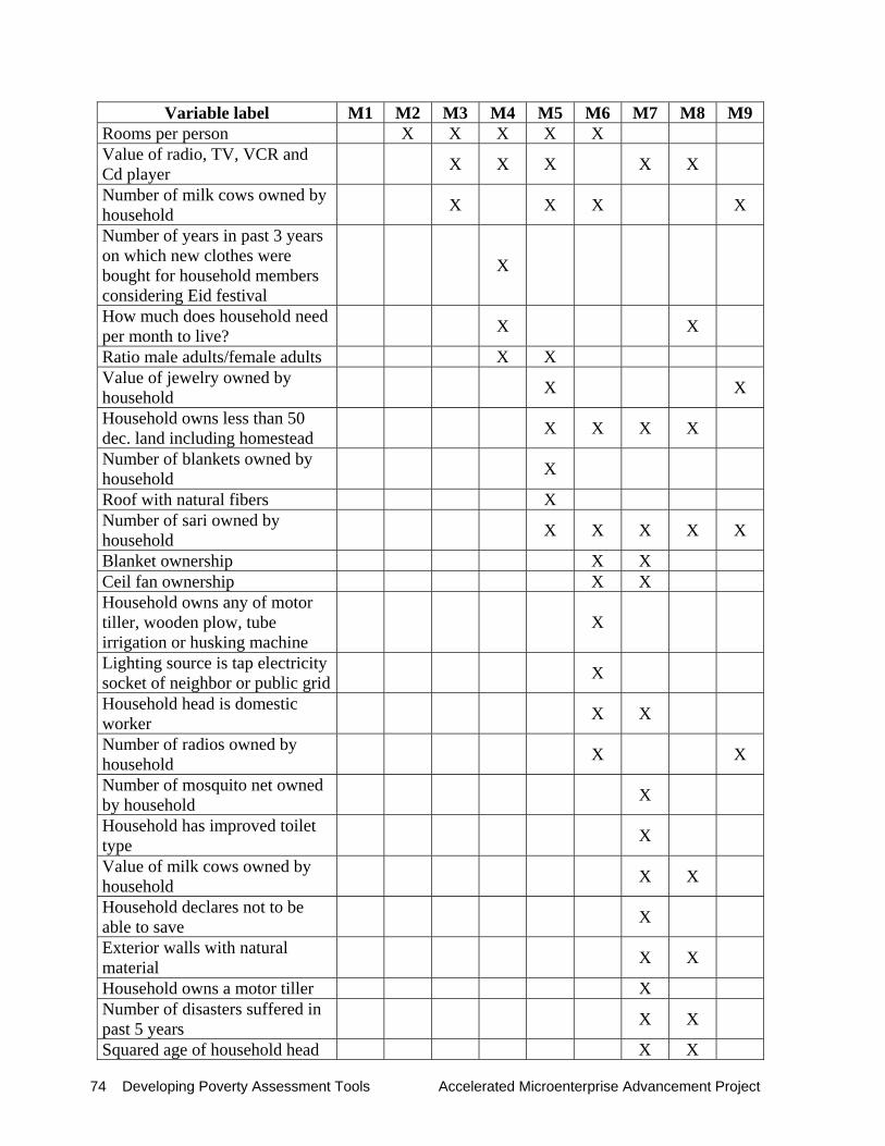
74 Developing Poverty Assessment Tools Accelerated Microenterprise Advancement Project
Variable label M1 M2 M3 M4 M5 M6 M7 M8 M9 Rooms per person X X X X X Value of radio, TV, VCR and Cd player X X X X X
Number of milk cows owned by household X X X X
Number of years in past 3 years on which new clothes were bought for household members considering Eid festival
X
How much does household need per month to live? X X
Ratio male adults/female adults X X Value of jewelry owned by household X X
Household owns less than 50 dec. land including homestead X X X X
Number of blankets owned by household X
Roof with natural fibers X Number of sari owned by household X X X X X
Blanket ownership X X Ceil fan ownership X X Household owns any of motor tiller, wooden plow, tube irrigation or husking machine
X
Lighting source is tap electricity socket of neighbor or public grid X
Household head is domestic worker X X
Number of radios owned by household X X
Number of mosquito net owned by household X
Household has improved toilet type X
Value of milk cows owned by household X X
Household declares not to be able to save X
Exterior walls with natural material X X
Household owns a motor tiller X Number of disasters suffered in past 5 years X X
Squared age of household head X X
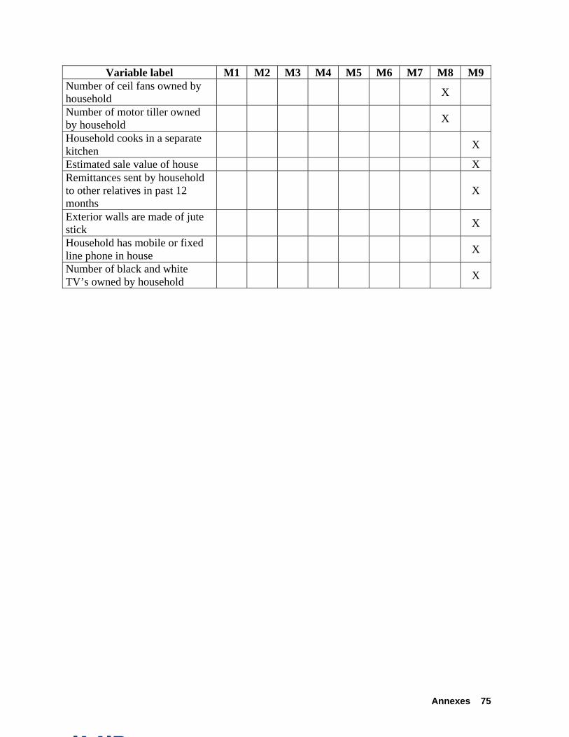
Annexes 75
Variable label M1 M2 M3 M4 M5 M6 M7 M8 M9 Number of ceil fans owned by household X
Number of motor tiller owned by household X
Household cooks in a separate kitchen X
Estimated sale value of house X Remittances sent by household to other relatives in past 12 months
X
Exterior walls are made of jute stick X
Household has mobile or fixed line phone in house X
Number of black and white TV’s owned by household X
76 Developing Poverty Assessment Tools Accelerated Microenterprise Advancement Project
Endnotes 1 This report consists of original work and data analysis. Citations of entire paragraphs or tables in published material by other authors is only permitted after prior consent with the authors and the IRIS Center. The cleaning and processing of data, as well as the entire analysis presented in this report, was carried out at the Institute of Rural Development, University of Göttingen, Germany. We gratefully acknowledge the valuable comments and support given by the IRIS project members, particularly Thierry van Bastelaer, Omar Azfar, Tresja Denysenko, Kate Druschel, and Lauren Hendricks. The input by the SEEP Network and its Poverty Assessment Working Group, the Advisory Panel for the Developing Poverty Assessment Tools project, and the USAID is gratefully acknowledged. In particular, Christian Grootaert provided valuable comments and advice during all phases of the field research and data analysis, especially also with regard to the choice of regression technique and the presentation of results. We are also grateful to Don Sillers, Thierry van Bastelear, Jonathan Murdoch and Christian Grootaert for valuable comments on an earlier draft. The analysis on accuracy of Participatory Wealth Ranking has been carried out by Joseph Feulefack, an M.Sc. student at the Institute of Rural Development who carries out his M.Sc research on this topic. Peter Kao, a Ph.D. candidate of the Institute of Statistics at the University of Göttingen programmed SAS routines for the regression analysis. All remaining error are ours. 2 Contact Information: Data Analysis and Technical Assistance (DATA) Ltd., 8/4, Block A (Unit 2), Lalmatia, Dhaka – 1207, Bangladesh, Phone: (880-2) 8114870, 9111328, 9129644, Fax: (880-2) 9111328, E-mail: [email protected], DATA on Web: http://www.databd.org 3 See World Bank (2004), World Development Indicators. www.worldbank.org/data/wdi2004/pdfs/table2-5.pdf 4 Purchasing power parity exchange rates between US-Dollar and other currencies are available at www.worldbank.org/povmonitor/ppp1993.htm. 5 For monthly inflation rates, we use those published by the Bangladesh Bureau of Statistics. We plan to update the calculation of the international poverty line, expressed in local currency, when new data on CPI changes for the period March 2003 to March 2004 become available. 6 The best sets of poverty indicators identified on each of the nine models refer to the combination of 5, 10 or 15 indicators selected by the SAS-MAXR procedure. 7 The term regressor or poverty indicator are interchangeably used in this document. Literally speaking, they refer to a certain type of variable used in the regression. The regressors can be derived from one or many questions from the composite questionnaire. For example, some regressors or poverty indicators are directly computed from the variable obtained in the survey, such as the age of the household head. Other regressors require computation (using info from one or several questions) as they are not directly asked but are derived from the responses to the questions asked. An example is the size of the household (which is calculated from the information given in section B of the questionnaire). 8 In case a monetary variable had a value of zero Taka given by the respondent, this was replaced. For the case of zeroes as original monetary values, these were replaced by the value of one pro mille of the mean in order to compute the natural logarithm. 9 Using the MAXR function of SAS, we selected in a prior model the best regressor among 13 expenditure categories (referring to questions C1 to C12 as well as clothing expenditures of section B of the composite questionnaire) and expenditure derived variables (i. e. percentage share of food expenditures in total household expenditures). The inclusion of only the single best of the expenditure categories was done so as to avoid dominance of expenditure variables in subsequent models. 10 It is therefore important to consider the framework of incentives for when, where, and by whom a poverty assessment is carried out (incentives for the respondent as well as the interviewer). The following quote taken from an email by Jan Maes (Trickle Up Program) highlights some of the issues involved here: “One way of preventing clients from exaggerating their poverty or otherwise responding in a way they think ’would help their case,’ is to conduct the poverty assessment survey after loan approval rather than to use it as part of the approval process. In other words, this implies that the USAID certified tools will be ex post poverty assessment tools rather than ex ante poverty targeting tools”… “If you use the assessment as part of the loan application or selection process, you will have to interview all potential clients, including of course those who ’fail the poverty test’. On the downside, since you only get your poverty results after clients have already entered the program, you might learn when it is already too late that you are not reaching the poorest.”
Endnotes 77
11 The managing directors of DATA were asked to rate the verifiability of each of the indicators on a scale from 1 to 5 where 1 is very difficult or impossible to verify, and 5 stands for easy verifiability. In Annex D, we list the rating given by the survey firm DATA in Bangladesh. In model 7, we include only the regressors that have been rated as easily verifiable (i.e. a score of 5). 12 These variables were identified by the SAS-MAXR procedure as the strongest variables among all subjective variables which were excluded in Model 5. 13 In his paper, Mark Schreiner differentiates seven aspects of loan size, including outstanding debt and repayment amount per time period that could be alternatively used as a tool to predict poverty. In the following, we focus on testing the accuracy of loan size since this indicator is widely used among practitioners and reported in publications such as the Microbanking Bulletin; in addition the current USAID requirement is to use loan size as a proxy for determining the poverty level of microfinance clients. 14 This section is an excerpt of a forthcoming paper by Zeller et al. (2004). 15 Similar to the use of the term BEST in chapter 3 for the set of BEST5 regressors for example, the term BEST does not imply a value judgement. Our method of searching for the best score has been applied here to calibrate PWR so as to achieve the highest overall accuracy. However, our method could also be used to find the BEST score minimizing leakage or undercoverage, or the other accuracy levels. 16 We verified that in none of the hamlets of these 7 villages, the critical number of 10 percent of highly inconsistent cards is reached. 17 Alternatively, new reference groups may be formed to obtain repeat rankings until more consistent scores are found, up to the limit of five total reference groups. As mentioned above, additional reference groups can be formed without, however, exceeding the maximum of five (Gibbons & Simanowitz with Nkuna, 1999, p.61). However, this was not done during the PWR exercise, and we are only left with the option to exclude these two hamlets from the data set for accuracy analysis of PWR. 18 We also computed the accuracy results using the sample of 320 households. The level of accuracy is marginally lower than the one for 293 households. 19 The term BEST score refers simply to the score that maximizes accuracy of a calibrated PWR tool. The term BEST score is not meant as a value judgement. With our best score method, one can also identify alternative BEST scores that maximize accuracy among the poor or accuracy among the non-poor, or that minimize leakage or undercoverage. For this reason, we provide the accuracy results for a range of scores so as to display the comparative advantages of other scores with respect to the all five performance criteria. 20 The very low accuracy among the very poor could be significantly reduced if the score chosen for calibration of the PWR tool would be lower. We therefore present also the accuracy results in this and the next section for other scores. Table 4.2.2.4 shows, for example, that a PWR tool calibrated with a score of 80 (i.e. identifying households with a score of 80 or above as very poor) would reach a much higher accuracy among the very poor of 73.34 percent. However, choosing a lower score implies that overall accuracy and the accuracy among the not very poor declines to 67.7 and 64.34 percent, respectively. 21 The loss in accuracy over larger geographical units implies a lower accuracy for a truly national sample. As the nation in this section reflects only data from 4 districts, the true result of PWR at a full national scale comparable to the sample of 799 households analyzed in chapter 3 is likely to be lower than the 70.3 percent obtained for the sample of 293 households. 22 This is simply noted as a possibility. The descriptive results shown in the table do not provide any statistically valid evidence of impact. 23 We will further investigate this result in the accuracy tests for Kazakhstan, Peru and Uganda. 24 This imbalance between the two types of accuracy could be potentially reduced, for example, by two-step regression models developed by Grootaert et al. (1998). However, the computational costs of these models will be higher than ordinary least squares models.