DEVELOPING A RUN-TIME COUPLING BETWEEN ESP-R AND …
148
UNIVERSITÉ DE MONTRÉAL DEVELOPING A RUN-TIME COUPLING BETWEEN ESP-R AND TRNSYS ROMAIN JOST DÉPARTEMENT DE GÉNIE MÉCANIQUE ÉCOLE POLYTECHNIQUE DE MONTRÉAL MÉMOIRE PRÉSENTÉ EN VUE DE L’OBTENTION DU DIPLÔME DE MAÎTRISE ÈS SCIENCES APPLIQUÉES (GÉNIE MÉCANIQUE) DÉCEMBRE 2012 © Romain Jost, 2012.
Transcript of DEVELOPING A RUN-TIME COUPLING BETWEEN ESP-R AND …

UNIVERSITÉ DE MONTRÉAL
DEVELOPING A RUN-TIME COUPLING BETWEEN ESP-R AND TRNSYS
ROMAIN JOST
DÉPARTEMENT DE GÉNIE MÉCANIQUE
ÉCOLE POLYTECHNIQUE DE MONTRÉAL
MÉMOIRE PRÉSENTÉ EN VUE DE L’OBTENTION
DU DIPLÔME DE MAÎTRISE ÈS SCIENCES APPLIQUÉES
(GÉNIE MÉCANIQUE)
DÉCEMBRE 2012
© Romain Jost, 2012.

UNIVERSITÉ DE MONTRÉAL
ÉCOLE POLYTECHNIQUE DE MONTRÉAL
Ce mémoire intitulé:
DEVELOPING A RUN-TIME COUPLING BETWEEN TRNSYS AND ESP-R
présenté par : JOST Romain
en vue de l’obtention du diplôme de : Maîtrise ès sciences appliquées
a été dûment accepté par le jury d’examen constitué de :
M. BERNIER Michel, Ph.D., président
M. KUMMERT Michaël, Ph.D., membre et directeur de recherche
M. BEAUSOLEIL-MORRISON Ian, Ph.D., membre

iii
ACKNOWLEDGEMENTS
Je tiens à remercier tout particulièrement Michaël Kummert, mon directeur de recherche, pour la
disponibilité, le soutien ainsi que la confiance qu'il m'a accordés tout au long de ces deux années
de maîtrise.
I am grateful to all the co-simulator project Team members. A special thanks goes to Francesca
Macdonald for her dynamism and in memory of these long days spent on debugging the coupling
together. I would like to thank Tim Mcdowell for his warm welcome in Madison and his support
in helping me getting to know the dark parts of TRNSYS. I wish to thank Ian Beausoleil-
Morrison and Alex Ferguson for their contributions and management of the project. Nothing of
this would have been possible without them.
Je voudrais remercier également tous les MecBats avec qui j'ai passé deux ans inoubliables à
Polytechnique: Aurélie Verstraete, Katherine D'Avignon, Marilyne Rancourt-Ouimet, Marion
Perez, Antoine Courchesne-Tardif, Benoit Delcroix, François Adam, Humberto Quintana,
Massimo Cimmino, Mathieu Lévesque, Matthieu Grand, ainsi que Michel Bernier.
I wish to thank Westphal Jean-Paul pour m'avoir enseigné le bon usage des "therefore" dans
l'écriture de ce mémoire et ses autres nombreuses corrections.
Merci à mes parents pour leurs encouragements ainsi qu'à tous ceux que j'ai côtoyés et qui m'ont
soutenu durant toute la durée de ce travail.

iv
RESUME
Dans le cadre de la réduction de l'énergie consommée par les bâtiments, il est essentiel d'être
rigoureux dans leur modélisation. Pour ce faire, un grand nombre de logiciels de simulation
existe, mais, ces outils sont pour la plupart spécialisés dans un domaine particulier et ne
permettent pas toujours de réaliser une analyse complète. Étant donné que tous les domaines
(chauffage, climatisation, ventilation, éclairage, acoustique) sont interdépendants, il n'existe pas
de plateforme de simulation permettant de couvrir toutes les particularités d'un système avec la
même flexibilité, et il est nécessaire de procéder à des combinaisons ou des couplages de
logiciels. Ce mémoire décrit la réalisation d'un couplage au niveau de l'exécution entre TRNSYS
et ESP-r.
Afin de réduire au maximum les modifications apportées aux codes sources et façonner un outil
durable face au développement de chacun des deux logiciels dans le futur, le couplage se fait
principalement à l’aide de nouveaux composants recevant et envoyant des données à l'autre
programme. L'échange de données est réalisé par une structure à DLLs multiples. En plus de
celles de TRNSYS et ESP-r, une troisième DLL chargée d'appeler les deux autres et de contrôler
l'échange d'information a été créée. Celle-ci supervise également le contrôle de la convergence et
assure l'avancement simultané des deux programmes. Cette DLL qui joue le rôle d’intermédiaire
entre les deux logiciels (middleware) est appelée l’Harmonizer.
Une nouvelle catégorie de composants a été mise en place pour le logiciel TRNSYS. Il s'agit des
Types Échangeurs de Données (Data Exchanger Types). Ces composants fonctionnent de
manière identique aux Types classiques en communiquant à travers leurs entrées et sorties, mais
ils sont également capables de forcer le solveur à poursuivre les itérations d'un pas de temps.
Cette fonctionnalité est essentielle afin d'obliger TRNSYS à faire de nouveaux calculs lorsque
qu'il y a convergence au niveau interne mais que ce n'est pas le cas pour l'autre logiciel. Un
composant de cette nouvelle catégorie, appelé Type 130, a été créé spécialement pour le couplage
avec ESP-r. Ce dernier assure la liaison et l'échange de données entre l'Harmonizer d'une part et
les composants du système dans TRNSYS de l'autre.
Du point de vue de l'utilisateur, il n'y a que peu de changements entre le fait de réaliser un modèle
pour une co-simulation et celui pour une simulation n'utilisant qu'un seul logiciel. Les fichiers
d'entrée et de sortie sont identiques à ceux d'une simulation standard, et ce pour les deux

v
logiciels. L'unique fichier additionnel à configurer est le fichier d'entrée de l'Harmonizer
contenant les paramètres de la co-simulation.
Ce mémoire décrit le travail réalisée par l’équipe du projet et les contributions spécifiques de
l’auteur sont identifiées dans le texte.

vi
ABSTRACT
Rigorous modeling is essential to design buildings and deliver the next advances in energy
efficiency and on-site renewable energy production. A great variety of energy simulation
programs exists but they are, for the most part, specialized in one particular domain and they do
not allow a complete analysis. Because all domains (heating, cooling, ventilation, lighting,
acoustic) are interconnected and there is no global simulation environment existing that covers all
of the system particularities with the same flexibility, it is often appropriate to proceed with
software combination and/or coupling. This Master thesis describes the implementation of a run-
time coupling between TRNSYS and ESP-r.
In order to minimize the modifications to the source codes and create a tool able to support future
development of each program, new components that receive and pass data to the other program
were implemented in the two software programs. A multi DLL structure enables the coupling and
exchange of information. A third piece of software, the Harmonizer, launches TRNSYS and ESP-
r DLLS and manages the exchange of data. It is also responsible of the convergence handling and
controls that both programs march through time together time step after time step.
A new category of components, the Data Exchanger Types was implemented in TRNSYS. These
components can work as standard TRNSYS Types and exchange data through their inputs and
outputs but they can also impose the solver to continue iterating. This capability is essential to
force TRNSYS to do more calculations at a specific time step when it has converged but co-
simulation convergence requires more iterations. A component of this new category, Type 130,
was created specifically for the coupling with ESP-r. Type 130 exchanges data with the
Harmonizer on one side and with the TRNSYS network of Types on the other side.
Testing of basic data exchange validates the data exchange method and the coupling. The co-
simulator is able to simulate a complete system with a building modeled in ESP-r and the energy
system in TRNSYS.
On the user perspective, there are few changes in implementing a co-simulation model in
comparison to a simple simulation model using only one program. Users with some knowledge
of both programs will be familiar with the steps required to perform a co-simulation. The input

vii
and output files are the same for the two programs as a standard simulation. Settings of the co-
simulation are defined in the Harmonizer input.
This Master Thesis describes the work of the project team, referred to as the Design Team in the
text. Specific contributions from the author are identified in the document.

viii
TABLE OF CONTENT
ACKNOWLEDGEMENTS .......................................................................................................... III
RÉSUMÉ ....................................................................................................................................... IV
ABSTRACT .................................................................................................................................. VI
TABLE OF CONTENT ............................................................................................................. VIII
LIST OF TABLES .......................................................................................................................XII
LIST OF FIGURES .................................................................................................................... XIII
LIST OF ABBREVIATIONS .................................................................................................... XVI
INTRODUCTION ........................................................................................................................... 1
CHAPTER 1 LITERATURE REVIEW .................................................................................... 3
1.1 Building simulation .......................................................................................................... 3
1.1.1 Net Zero Energy Buildings .......................................................................................... 3
1.1.2 Integrated simulations .................................................................................................. 4
1.1.3 TRNSYS and ESP-r ..................................................................................................... 6
1.2 Internal coupling .............................................................................................................. 9
1.3 External coupling ........................................................................................................... 10
1.3.1 The Neutral Model Format ......................................................................................... 11
1.3.2 Sequential coupling .................................................................................................... 12
1.3.3 Run-time coupling ...................................................................................................... 13
1.4 Implementation of a run-time coupling .......................................................................... 15
1.4.1 Master/slave strategy .................................................................................................. 15
1.4.2 Middleware ................................................................................................................. 16
CHAPTER 2 ESP-R, TRNSYS AND COUPLING METHODOLOGIES ............................. 18
2.1 ESP-r methodologies ...................................................................................................... 18

ix
2.1.1 Building thermal domain ............................................................................................ 19
2.1.2 Plant domain ............................................................................................................... 21
2.1.3 Electrical domain ........................................................................................................ 23
2.2 TRNSYS methodologies ................................................................................................ 23
2.2.1 Overview .................................................................................................................... 24
2.2.2 TRNSYS Types .......................................................................................................... 26
2.2.3 Solver ......................................................................................................................... 28
2.2.4 Categories of Types .................................................................................................... 30
2.3 Co-simulation approach ................................................................................................. 31
2.3.1 Run time coupling ...................................................................................................... 31
2.3.2 Middleware ................................................................................................................. 33
2.3.3 Exchange of data ........................................................................................................ 34
2.3.4 Harmonizer functions ................................................................................................. 37
CHAPTER 3 SOURCE CODE MODIFICATIONS ............................................................... 40
3.1 Modifications in ESP-r source code ............................................................................... 40
3.1.1 Coupling components ................................................................................................. 41
3.1.2 Coupling subroutine ................................................................................................... 42
3.2 TRNSYS: Creation of a new category of Types ............................................................ 42
3.2.1 Objectives ................................................................................................................... 43
3.2.2 Data exchanger Types ................................................................................................ 43
3.2.3 TRNSYS kernel main subroutines ............................................................................. 46
3.2.4 Modifications to the code ........................................................................................... 54
3.3 TYPE 130 ....................................................................................................................... 60
3.3.1 Generalities in Types coding ...................................................................................... 60

x
3.3.2 Type 130 communication process .............................................................................. 61
3.3.3 Type 130 inputs, outputs and parameters ................................................................... 63
3.3.4 Standard and test modes ............................................................................................. 64
3.3.5 Type 130 code ............................................................................................................ 65
CHAPTER 4 DEMONSTRATION AND TESTS .................................................................. 68
4.1 Preliminary tests ............................................................................................................. 68
4.1.1 External data transfer and iteration control ................................................................ 68
4.1.2 Data exchange with ESP-r (Test A) ........................................................................... 69
4.2 Water based heating system (test B) .............................................................................. 70
4.2.1 System tested .............................................................................................................. 70
4.2.2 ESP-r .......................................................................................................................... 71
4.2.3 Simulation using TRNSYS only ................................................................................ 71
4.2.4 Results analysis .......................................................................................................... 73
4.3 Air based heating system and humidity transfer (test D) ............................................... 75
4.3.1 No humidity source .................................................................................................... 76
4.3.2 Constant humidity source ........................................................................................... 78
4.4 House serviced by a DHW/space heating solar combi-system (test C) ......................... 80
4.4.1 System tested .............................................................................................................. 80
4.4.2 TRNSYS ..................................................................................................................... 82
4.4.3 ESP-r .......................................................................................................................... 85
4.4.4 Coupling settings ........................................................................................................ 86
4.4.5 Results analysis .......................................................................................................... 87
CHAPTER 5 USING THE ESP-R / TRNSYS CO-SIMULATOR ........................................ 95
5.1 Generalities ..................................................................................................................... 95

xi
5.2 Harmonizer input file ..................................................................................................... 96
5.3 ESP-r model ................................................................................................................... 97
5.4 TRNSYS model ............................................................................................................ 101
5.4.1 Creation of TRNSYS input file ................................................................................ 101
5.4.2 Type 130 Test mode ................................................................................................. 106
5.4.3 Note about controllers .............................................................................................. 107
5.5 Co-simulation ............................................................................................................... 108
5.5.1 Running a co-simulation .......................................................................................... 109
5.5.2 Results recovery ....................................................................................................... 110
CONCLUSION ........................................................................................................................... 112
BIBLIOGRAPHY ....................................................................................................................... 114
ANNEX 1 – ESP-R METHODOLOGIES .................................................................................. 117
ANNEX 2 – SOURCE CODE MODIFICATIONS IN TRNSYS .............................................. 118
ANNEX 3 – TYPE 130 CODE ................................................................................................... 125

xii
LIST OF TABLES
Table 2-1 Categories of Types ....................................................................................................... 31
Table 2-2 List of variables and types from the derived data structure ........................................... 36
Table 3-1 Arguments of Exec subroutine ....................................................................................... 49
Table 3-2 “Call” arrays .................................................................................................................. 52
Table 3-3 Arguments of Loopex subroutine ................................................................................... 53
Table 4-1 Radiator model parameters ............................................................................................ 72
Table 4-2 Description of radiator governing equation variables .................................................... 73
Table 4-3 Settings of Test D without humidity source .................................................................. 76
Table 4-4 Settings of Test D with Humidity source ....................................................................... 78
Table 4-5 Parameters of solar collectors ........................................................................................ 82
Table 4-6 Co-simulation parameters for Test C ............................................................................. 86
Table 4-7 Combi-system co-simulation results (annual simulation) ............................................. 87
Table 4-8 Description of energy transfers ...................................................................................... 89
Table 5-1 Constant values sent by Type 130 in test mode ........................................................... 107

xiii
LIST OF FIGURES
Figure 1-1 TRNSYS Simulation Studio ........................................................................................... 7
Figure 1-2 ESP-r Project Manager interface .................................................................................... 8
Figure 1-3 Couplings synthesis ...................................................................................................... 12
Figure 1-4 Run-time coupling strategies (Trcka, Wetter, & Hensen, 2009) .................................. 13
Figure 1-5 Loose coupling zig-zag ................................................................................................. 16
Figure 1-6 Interactions between the middleware and the programs .............................................. 17
Figure 2-1 ESP-r's partitioned solution approach (Beausoleil-Morrison, 2011) ............................ 18
Figure 2-2 ESP-r's building thermal domain finite difference ....................................................... 19
Figure 2-3 Heat balance for a zone air CV (Beausoleil-Morrison, 2011) ...................................... 20
Figure 2-4 Heat balance for intra-constructional CV (Beausoleil-Morrison, 2011) ...................... 21
Figure 2-5 Simulation Studio ......................................................................................................... 24
Figure 2-6 TRNBuild ..................................................................................................................... 25
Figure 2-7 TRNEdit interface and example of a TRNSED application ......................................... 26
Figure 2-8 TRNSYS Type and network topology ......................................................................... 27
Figure 2-9 Interactions between the main TRNSYS programs and files during a simulation ....... 28
Figure 2-10 TRNSYS solution methodology ................................................................................. 29
Figure 2-11 Sequence of calls to the different categories of Types ............................................... 30
Figure 2-12 Differences in run-time couplings .............................................................................. 32
Figure 2-13 Data flows between the Harmonizer and the coupled programs ................................ 33
Figure 2-14 Derived Data Structure ............................................................................................... 35
Figure 2-15 Interactions between the two programs and the Harmonizer (Macdonald, 2012)...... 39
Figure 3-1 Coupling components strategy to transfer data to the other program .......................... 40
Figure 3-2 TRNSYS Coupling Components .................................................................................. 41

xiv
Figure 3-3 Calling sequence with Category 6: Data exchanger Types .......................................... 45
Figure 3-4 Original post iterations process .................................................................................... 48
Figure 3-5 Modifications to the post iterations process ................................................................. 58
Figure 3-6 Network of Types including Type 130 ......................................................................... 62
Figure 3-7 Inputs and outputs organization.................................................................................... 63
Figure 3-8 Coupling components connections ............................................................................... 64
Figure 3-9 Summary of Type 130 calls and operations ................................................................. 67
Figure 4-1 Schematic of test B system ........................................................................................... 70
Figure 4-2 Overview and front view of BESTEST case 600 building ........................................... 71
Figure 4-3 TRNSYS only simulation for Test B............................................................................ 72
Figure 4-4 Comparison of zone air temperature for two winter days ............................................ 73
Figure 4-5 Evolution of the zone air temperature for the two test cases B1 (right) and B2 (left) . 74
Figure 4-6 Evolution of the zone air temperature and water flow rate with a PID controller ....... 75
Figure 4-7 Schematic of test D system without humidity source .................................................. 76
Figure 4-8 - Transient state humidity ratios ................................................................................... 77
Figure 4-9 - Differences between HR send to the zone and HR of the zone ................................. 77
Figure 4-10 Schematic of test D system with constant humidity source ....................................... 78
Figure 4-11 Schematic of test C system ......................................................................................... 81
Figure 4-12 TRNSYS simulation for Test C .................................................................................. 82
Figure 4-13 DHW load profile ....................................................................................................... 83
Figure 4-14 Type 130 connections ................................................................................................. 85
Figure 4-15 Zone house model in ESP-r ........................................................................................ 85
Figure 4-16 Connections at the interface between the two programs ............................................ 86
Figure 4-17 Number of iterations per time-step ............................................................................. 88

xv
Figure 4-18 Energy transfers in the system .................................................................................... 88
Figure 4-19 Space heating solar fraction ........................................................................................ 92
Figure 4-20 Domestic hot water solar fraction ............................................................................... 92
Figure 4-21 System total solar fraction .......................................................................................... 93
Figure 5-1 Co-simulator's input and output files ............................................................................ 95
Figure 5-2 Harmonizer input file ................................................................................................... 96
Figure 5-3 ESP-r input file ............................................................................................................. 98
Figure 5-4 Example of a plant system including coupling components ........................................ 99
Figure 5-5 Coupling components connections: HCC on the left and ACC on the right
(Macdonald, 2012) ............................................................................................................... 100
Figure 5-6 Example of connections for ACCs (blue) and HCCs (red) ........................................ 100
Figure 5-7 TRNSYS input file ..................................................................................................... 101
Figure 5-8 TRNSYS network of Types ........................................................................................ 102
Figure 5-9 Addition of Type 130 to the network of Types .......................................................... 103
Figure 5-10 Type 130 parameters settings ................................................................................... 103
Figure 5-11 TRNSYS network of Types with Type 130 ............................................................. 104
Figure 5-12 Simulation parameters .............................................................................................. 105
Figure 5-13 Creation of TRNSYS input file ................................................................................ 106
Figure 5-14 Co-simulation output files ........................................................................................ 110

xvi
LIST OF ABBREVIATIONS
ACC Air Coupling Component
BCVTB Building Control Virtual Test Bed
BPS Building Performance Simulation
CV Control Volume
DDS Derived Data Structure
DLL Dynamic-Link Library
FCC Fluid Coupling Component
HCC Hydronic Coupling Component
HR Humidity Ratio
HVAC Heating, Ventilation and Air-Conditioning
IAQ Indoor Air Quality
NMF Neutral Model Format
NZEB Net Zero Energy Building
OS Operating System
PID Proportional Integral Derivative
PV Photovoltaic
TCC TRNSYS Coupling Component

1
INTRODUCTION
Designing the next generation of energy efficient buildings with on-site renewable energy
production to meet the “Net Zero Energy” target requires the use of integrated simulation tools
capable of dealing with the level of complexity in the building and the associated mechanical and
electrical systems.
A great variety of efficient Building Performance Simulation (BPS) tools exist on the market but
they are, for the most part, specialized in one particular domain and lack flexibility or capabilities
in other domains. This may affect the accuracy of simulations results as it is sometimes difficult
to perform a whole system analysis with one tool. ESP-r and TRNSYS are both powerful
simulation programs but their different implementation approaches gave them different strengths.
ESP-r is particularly efficient in modeling building physics whereas TRNSYS is more flexible in
treating elaborated mechanical and electrical systems. Because all domains (heating, cooling,
ventilation, lighting, acoustic) are interconnected and there is no global simulation environment
existing that covers all particularities of a system with the same flexibility, combining or
coupling simulation programs is often required.
This document presents the work on the development of a run-time coupling between TRNSYS
and ESP-r. With funding and guidance from Natural Resources Canada, a Design Team
composed of 6 people from Carleton University, Ottawa, École Polytechnique de Montréal, and
Thermal Energy System Specialists (TESS), Madison (USA), completed this project. Tasks were
divided between the members: the Carleton University part of the team worked on the
implementation of the coupling on the ESP-r side and on the implementation of the middleware
(known as the Harmonizer), team members from Polytechnique Montréal and TESS carried out
modifications to the TRNSYS source code. The whole Design Team was involved during all
phases of the project and provided inputs to development work and to the overall coupling
strategy, under the supervision of the project leader at Carleton University. This Master thesis
describes the methodology and results of the project, with more emphasis on the TRNSYS side.
The specific contributions of the author, who was the lead developer for TRNSYS source code
changes, are identified in the text.

2
Thesis organization
First, this document presents Building Performance Simulation combinations and couplings
described in the literature. The main approaches are compared. Chapter 1 gives an overview of
the couplings methods from basic links and collecting external data to integration of source code
and more complex run-time coupling. Chapter 2 presents the calculation methodologies of
TRNSYS and ESP-r and a description of the co-simulation approach selected by the Design
Team. Chapter 3 details the implementation of the coupling and the modifications to each
program source code. The ESP-r part is briefly commented, while TRNSYS source code changes
are presented in details with the source code provided in an Annex.
Chapter 4 reports on the various tests that were performed to confirm the proper operation and
the usefulness of the proposed co-simulator. Results demonstrating the coupling capabilities from
the very basic data exchange tests to complete co-simulations are presented there. Chapter 5
describes how to perform co-simulations from a user perspective, and leads to the final
conclusions of this work.

3
CHAPTER 1 LITERATURE REVIEW
This introductory chapter presents an overview of the current work in building performance
simulation and couplings between software programs. First, the need for integrating building
simulation programs and different approaches are presented. Then, different coupling methods
are discussed.
1.1 Building simulation
The design of buildings and mechanical systems aims at saving energy while maintaining or
improving occupant comfort. Integrated Building Performance Simulation (BPS) tools play an
important role in assessing the energy and economic performance of design options. They must
be efficient and adapted to more and more demanding building standards, codes and certification
programs. The end of the section presents two of the major programs in that domain, TRNSYS
and ESP-r.
1.1.1 Net Zero Energy Buildings
Design of buildings in the near future will be oriented towards the Net Zero Energy Building
(NZEB) target. Stricter energy efficiency regulations are already taking shape for the next
decades. In the USA, the goal of net zero for every new commercial building is set to 2030 by the
Energy Independence and Security Act of 2007 (EISA 2007). The European Union is even more
demanding in the reduction of energy consumption with the Energy Performance of Building
Directive (EPBD) that imposes a neutral energy balance for every new construction by 2020.
These texts are ambitious, however they lack precision on the definition of Net Zero Energy
buildings, as well as on the methodology to design those types of buildings (Marszal et al., 2011).
Currently, several definitions of NZEB exists (Torcellini, Pless, & Deru, 2006) but in order to
apply these new laws, a rigorous design methodology will be needed. This will also require the
creation of new buildings and systems simulation tools and/or modifications of the current ones
to respond efficiently to these energy saving constraints.

4
Several methods of defining the total energy balance of buildings already exist. The majority uses
the primary energy consumption in their calculations. They differ for example on the period of
simulation: they mostly consider a period of one year but this period can vary from a month to
the entire life cycle. A few of these approaches only consider thermal and electrical energy used
to operate the building, while others extend the energy balance to account for the energy required
during the construction process (including embodied energy for all construction materials). A
commonly used indicator of the net zero energy target is the ratio between the building energy
consumption and the on-site renewable energy production. There is no consensus on a “best”
methodology at this stage, each of them focuses on slightly different aspects of the problem. The
design of NZEBs and the evaluation of their performance must be adapted to the selected
methodology.
BPS tools must be adapted to these requirements and allow to improve energy efficiency at the
building level, as well as to integrate advanced Heating, Ventilation and Air-Conditioning
(HVAC) systems and on-site renewable energy systems.
1.1.2 Integrated simulations
Rigorous modeling is essential to design buildings that will meet the very ambitious energy
efficiency targets described above. It is essential to treat buildings and systems, at the same time
to get the best optimization (Hensen, Djunaedy, Radošević, & Yahiaoui, 2004). Using a systemic
modeling approach during the design phase, allows harmonizing all of the key domains of
building construction from the engineering part to the architectural part. This leads to a design
optimizing both the energy consumption and the comfort of occupants.
Bazilian et al. (2001) illustrated the need of integrated simulations in modeling co-generation
photovoltaic collectors and the strong link between architecture and system design. A façade
configuration with pre-heating of the supplied air is presented by the author who explained that
such a system would also impact substantially the architectural domain. It is therefore necessary
to tackle every domain at the same time. Although several existing systems have proved the
efficiency of that type of collectors, more detailed tests must be performed. The lack of modeling
tools capable of performing holistic simulations is a barrier to research projects in that field. A

5
great variety of building simulation programs exist but they are, for the most part, specialized in
one particular domain and they do not allow a complete analysis. All domains (heating, cooling,
ventilation, lighting, and acoustics) are interconnected. Considering that there is no global
simulation environment that covers all of the system particularities with the same flexibility,
researchers and practitioners must resort to software combination and/or coupling (Citherlet,
Clarke, & Hand, 2001). There are four possible strategies:
- Stand-alone programs
In this case, a new simulation has to be created for every particular domain of the analyzed
system, each time using different software. Thus, this leads to redundancy issues and it can be
very fastidious as every time design parameters change in a domain, all the simulations have to
be modified and re-run another time. Another constraint for that kind of technique is that the user
has to be familiar with all the different programs used.
- Interoperable programs
The programs share the same source of information. This can be done following two approaches:
a. Exchange of an entire model or a part of the model
b. Sharing of the model: each program uses information it needs from the common and
unique model.
The second approach removes the redundancy but, in any case, the user needs to be familiar with
all the programs as well. Although there can be a loss of time dealing with all the different
simulating tools, we are closer to the reality of a global project. This strategy clearly represents
the interactions between all the actors: engineer, architect, etc.
- Integrated programs
In this scenario, several domains are modeled and simulated with the same program. The
evolution of the program is simplified as it does not depend on other applications. Moreover it
does not need any data exchange format and necessitates only one model grouping all the project
information.
- Coupled programs
The users have to be familiar with both tools in this case too. Calculations are done
simultaneously by two or more programs that also exchange data. Several possibilities of

6
couplings exist and they will be presented below. This solution offers the best flexibility to the
users as it gives them the possibility to benefit from the new functionalities added to the coupled
programs.
1.1.3 TRNSYS and ESP-r
Simulating buildings and energy systems in a global approach can be performed efficiently by
coupling existing programs specialized in different domains. This requires to choose appropriate
programs, not only powerful in their specific domain but also complementary. Two different
programs that seem to satisfy these conditions are presented briefly below.
a. TRNSYS
TRNSYS (TRaNsient System Simulation program) is a complete, modular and flexible program
for systems simulations (Klein et al., 2010; Keilholz, 2002). The program allows modeling from
simple to very complex mechanical plants with varied control systems. The standard libraries
contain around 60 components in different domains: HVAC, controls, storage, solar equipment,
etc. This list can be completed by additional libraries but also custom-made components that
users can create themselves, requiring some Fortran, C or C++ coding skills. TRNSYS is
customizable, can be expanded relatively easily, and it can simulate a large number of very
specific systems. In addition, it has a user friendly interface for generating projects (Figure 1-1).
Components used in the simulation are selected and added to the workspace by a drag-and-drop
process before being connected and setup by the user.

7
Figure 1-1 TRNSYS Simulation Studio
The simulation environment allows modeling multi-zone buildings. Another possibility of the
software is to create, via a specialized editor, redistributable applications. It is particularly
intended to develop simplified simulation tools, which can then be freely distributed to users who
do not possess a TRNSYS license (Klein et al., 2010).
b. ESP-r
ESP-r is an Open-Source energy modeling program for buildings. Dealing with thermal, acoustic
and energy performance, it is a comprehensive integrated energy modeling tool. It helps reducing
energy use and emissions, and optimizing the occupant comfort. The source code base can be
compiled to run the program on several operating systems: Linux, MacOS, Windows/Cygwin and
Windows.
After 30 years of development, ESP-r is a powerful engine (Clarke, 2001) which has proved to be
very efficient in the modeling of buildings (Strachan, Kokogiannakis, & Macdonald, 2008).
Nonetheless, the program lacks of flexibility when it comes to simulate mechanical systems. This
may prevent users from addressing the design of global systems (building + HVAC components).
The configuration of controls can be a very complex task. Moreover ESP-r does not have a large
list of energy systems components as we can find in other simulation programs such as TRNSYS.

8
Figure 1-2 ESP-r Project Manager interface
Given the functionalities and specificities of TRNSYS and ESP-r, the flexibility of systems
network configuration for the first one and the comprehensive BPS aspects for the second one, a
coupling of these complimentary tools would provide results with increased value to those
obtained with each individual program.
a. Comparison of ESP-r and TRNSYS
ESP-r and TRNSYS are both tools that allow running dynamic simulations for buildings and
energy systems but they have different modeling approaches. Based on a report contrasting the
capabilities of several building energy performance simulation programs (Crawley, Hand,
Kummert, & Griffith, 2005), a comparison giving a more precise review of the strengths and
weaknesses of two programs is presented below.
The most rigorous program in the treatment of the building physics is ESP-r. The program
integrates features that are not available in TRNSYS. It uses multi-sided polygons to define
constructive elements. It also handles CFD modeling. When it comes to implement very specific
types of constructive solutions, ESP-r presents a wide range of materials with models of phase

9
change materials or transparent insulation. Moreover, ESP-r has the ability to simulate
daylighting illumination and controls with its link to Radiance. With all these capabilities, ESP-r
possesses more than TRNSYS the comprehensive BPS aspects.
TRNSYS has a larger library of components than ESP-r. This is particularly the case for primary
HVAC components (boilers, chillers, etc.). It is also easier for the users to create new
components by developing personalized Types and add them to the existing list of components.
TRNSYS’s modular nature based on components (“Types”) also makes it easier to implement
specialized control strategies. The ability to develop new components relatively easily and the
flexibility offered in combining them into systems and in defining control strategies make
TRNSYS well suited to model innovative systems
1.2 Internal coupling
The first option to couple two programs is to combine their source codes. In most of the cases the
coupling is done by adding a part of one program code to another. This may be for instance a
component modeling a piece of mechanical equipment that we want to model in another
environment.
In 1999, Dorer and Weber integrated COMIS source code in TRNSYS. COMIS is a ventilation
and contaminants transport simulator for multi zone buildings. This coupling enables to take into
account the interaction of air flow rate and transport of contaminants in the modular systems and
buildings simulation program. Indoor Air Quality (IAQ) is closely interrelated with thermal
comfort and energy performance and must be considered in a holistic design approach. A new
component (Type 57) was added to TRNSYS with a re-implementation of the COMIS source
code. It is intended to work in combination with the thermal multizone building component
(Type 56) and exchange data (e.g. temperature, flow rate) every iteration, similarly to all
TRNSYS components connected through their inputs and outputs. While some convergence
problems were identified in case of an important stratification of the air in a zone, a study on
effects of night cooling on a building proved that the coupling allows new possibilities of
simulations and offers a better help to architectural conception (Dorer & Weber, 1999).

10
On the other hand, some of the existing TRNSYS components in the HVAC and electrical
domains have been integrated into other simulation tools. In 1991, Hensen re-implemented a
TRNSYS component (known as Type 260) modeling an aquastat controlled heater into ESP-r
(Hensen, 1991) The parameters/inputs/outputs structure of TRNSYS components had to be
adapted to the ESP-r engine methodologies. More recently, in 2009, a general method to convert
components from TRNSYS to ESP-r has been developed (Wang & Beausoleil-Morrison, 2009).
The tool, known as the “TRNSYS wrapper”, makes it easier to incorporate a TRNSYS Type in
ESP-r by compiling the code of the component with the source code of ESP-r. The coupling
approach used here is the process model interoperation, since both programs use the same model.
A few modifications to the source code are required but they have been minimized as much as
possible for this work. For someone who has skills in TRNSYS and ESP-r, creating a new
component with the “wrapper” based on the TRNSYS source code should only take a few hours,
which is reasonable considering that the solvers of the two programs use very different
methodologies. ESP-r solves a global matrix system whereas TRNSYS solve equations
sequentially, component by component.
Internal coupling helps to add new capabilities to programs by reusing other programs models,
but it requires substantial source code changes. It can only be performed by users knowledgeable
in the two programs and in computer programming. Another major drawback of the method is
that the source code embedded into the other program is decoupled from the original source code,
so that any enhancements or bug fixes will have to be adapted again.
1.3 External coupling
There are different strategies to implement an external data exchange between different
simulation programs. The choice can be driven by a variety of factors: the need of a small
simulation run time, the accuracy of the results, the amount of modifications to the source code.
The most common ways to implement externals couplings based on previous works are presented
and discussed below.

11
1.3.1 The Neutral Model Format
Prior to thinking of how the programs are going to communicate, it is important to define what is
going to be exchanged. Indeed, simulation programs often do not use the same format or units for
their model data. Software A may calculate energy in Joules while a software B would use Watt-
hours. The approach in modeling the same component can be also be completely different. A
radiator is for example modeled by a node in a state-space matrix in ESP-r, whereas in TRNSYS
it is a black box with a temperature and a flowrate as inputs and calculated flow temperature and
power as outputs. In another case we can have two programs simulating two separate aspects of a
model as acoustic and thermal effects. The model and its properties are the same for both
programs but data needed by each program to do its calculations may differ.
The concept of the Neutral Model Format (NMF) was created in order to simplify the data
sharing and compatibility (Nataf, 1995). The file gives all the information that characterizes a
system in a generic way. It contains systems of differential and algebraic equations describing the
model with a listing of all the variables. The name and description of the model and the variables
are also present in the NMF. The objective is to enable the sharing of the model file and exchange
of data between several programs. Translators are then in charge of collecting data needed by
each program and making the unit conversion if necessary.
The independent format may be more complicated to understand for an experienced programmer,
but the advantage of NMF is that it can be read more easily by a large number of programs. More
importantly, it allows the programmer to focus on the accuracy of the modeling rather than on
writing computer code. Several NMF components such as a solar collector, a multi-layer wall, a
thermal zone were created and have proven their efficiency. Vuolle and Bring also proposed a
whole library of NMF components regrouping zones, walls, windows and controllers (Vuolle &
Bring, 1995). Their work demonstrated that using NMFs reduce the implementation time and
improve the efficiency of simulations. Moreover the general model format appears to be a robust
and maintainable solution as it is completely separate from the development of the programs.

12
1.3.2 Sequential coupling
In a paper published in 2005, Djunaedy & Hensen gave an overview of the different possibilities
for coupling programs. Unlike internal coupling which is used in order to improve a software
program by adding new capabilities, external coupling is relevant when the objective is to share a
simulation between two existing programs. It can be the case in modeling different domains in
different programs. As shown in Figure 1-3, external couplings can be divided in two categories:
sequential couplings and run-time couplings. In the first category, one program is executed after
the other. The results obtained with the first program launched are then used in the simulation run
with the second program. To improve the precision of the results it can be necessary to repeat the
process a few times and use the results obtained with one program in the simulation run with the
other one.
Figure 1-3 Couplings synthesis
The advantage of an external coupling is that the source code of each program is already written,
tested and validated. Coupling the programs externally can save substantial time and money in
comparison to internal coupling which requires source code changes. This coupling method is
easier to maintain as both programs will benefit from bug fixes and enhancements by their own
developers.
External coupling
Internal coupling
Sequential Run-time
Loose Strong

13
1.3.3 Run-time coupling
The most complete way to implement an external coupling is to run the programs at the
same time and have them communicate during the simulation. This approach is known as run-
time coupling. Three possible strategies to implement run-time coupling are shown in Figure 1-4.
Strong coupling Loose coupling (zig-zag) Loose coupling (cross)
Figure 1-4 Run-time coupling strategies (Trcka, Wetter, & Hensen, 2009)
"The circles represent the subsystem’s state at a specific moment in simulation time. The dashed
arrows indicate which coupling data (time-step wise) are available to each subsystem before the
time-step calculation is performed. The full-line arrows indicate the update of state variables."
(Trcka et al., 2009)
- Loose coupling (zig-zag)
In loose couplings programs do their own calculations and exchange data only once per time-
step. Regarding "zig-zag" coupling (Trcka et al., 2009), one program is executed after the other.
E.g.: Program A begins and proceeds with its calculations for the first time-step. Once it has
converged, it sends its results to Program B that performs its iterations for the same time-step. In
the meantime Program A waits until Program B converges. When Program B is done with its
own calculations, it sends data back to Program A which proceeds to the second time-step. The
same procedure is executed for each time-step (Δt).

14
A coupling at the time-step level based on this approach has been made between ESP-r and the
lighting simulation program Radiance (Janak, 1999). At each time-step ESP-r calls Radiance and
provides it input data. ESP-r waits then until the end of Radiance's iterations, collects the results
and uses them in its simulation. Data transfer happens through a temporary text file where the
calculated internal illuminance is written by Radiance and read by ESP-r.
- Loose coupling (cross)
For that type of coupling the programs exchange data at the end of each time-step. These pieces
of information are then used as input data for the following time-step. Each program performs its
own calculations on its side and once the two programs have converged, they both send their
results to each other. “Cross” and "zig-zag" couplings deliver improved accuracy compared to
sequential coupling, because they exchange data at every time-step. In sequential coupling the
whole simulation is executed twice, once with one program and another time with the other. In
this particular example, the frequency of data exchange is one time per time-step, but it can be
extended to decrease the simulation running time. This will depend on the precision of the results
wanted (Trcka, 2008).
- Strong coupling
In a strong coupling implementation, there are iterations between the two programs at each time-
step (Trcka, Hensen, & Wijsman, 2006). The programs exchange data several times per time-step
until an overall convergence is reached. Once the whole system has converged the two programs
proceed separately to the next time-step and the same "double" procedure of iterations is done
until the end of the simulation. This method should deliver a better accuracy at the cost of
increased running time, as a higher frequency of the data exchange will result in more iterative
simulation calls. This strategy is mentioned in the literature but, according to our literature
survey, it has never been actually implemented between two or more complex Building
Performance Simulation (BPS) programs.

15
1.4 Implementation of a run-time coupling
A run-time-coupling is the best solution when existing programs are efficient in a certain domain
but not complete enough to be used for a comprehensive energy simulation. This process model
cooperation can be implemented in two different ways: the master/slave strategy or the addition
of a middleware.
1.4.1 Master/slave strategy
The choice of the co-simulation strategy implies to define which program will have the control of
the whole simulation, which program will wait for the other's data, which one is going to impose
input data to the other, etc. For the "master and slave" or "base program/external program"
approach one program has the control of the other. It is the case for the coupling between ESP-r
and Radiance (Janak, 1999) mentioned before where the lighting simulation program is
commanded by ESP-r. A coupling of TRNSYS and EnergyPlus realized in 2009 is also based on
this subordination relationship between the two programs. Figure 1-5 illustrates the interactions
between the two coupled programs and the differences of each program operations sequence for a
time-step (Trcka et al., 2009). The "master" program sends data to the "slave" program at the first
iteration of the time-step and then waits for the return of data. The "slave" program sends back
once it has converged for the time-step. This strategy is particularly adapted to the "zig-zag"
coupling coding as one program is executed after the other.

16
Figure 1-5 Loose coupling zig-zag
1.4.2 Middleware
Another concept of implementation of a run-time coupling that can be found in the literature is
the creation of an additional piece of software: the middleware. Also named "mediator" (Gamma,
Helm, Johnson, & Vlissides, 1995), its role is to centralize all the communication between the
coupled programs. The schematic of Figure 1-6 presents the interactions between all the
programs.
yesyes
TIM
E ST
EP O
PER
ATI
ON
S
First iteration of the time-step ?
Send data to B
Calculation of iteration n
A (master)A (master)
Receive data from B
First iteration calculation
Convergence ?
nono
yesyes
nono
yesyes
First iteration of the time-step ?
Receive data from A
Calculation of iteration n
B (slave)B (slave)
First iteration calculation
Convergence ?
nono
yesyes
nono
Send data to A
Proceed to next time-step
Proceed to next time-step

17
Figure 1-6 Interactions between the middleware and the programs
The middleware simplifies the data transfer handling. Instead of communicating with each other,
all programs exchange information with only one program that monitors fluxes of data. It is an
efficient way to centralize all the constraints and control functions in the middleware. Gamma et
al. (1995) described the simplification of the information exchange by "one to many interaction"
instead of "many to many interactions".
An example of the implementation of a middleware in an energy simulation programs coupling is
the Building Control Virtual Test Bed (Wetter, 2008, 2011). It is an interface of different
simulation tools enabling data exchange. It offers the possibility to link EnergyPlus to other tools
and it is therefore meant to be used for testing integrated buildings energy systems and controls.
The middleware has its own interface where the user can choose the co-simulation and controls
settings. It also has the functionality to analyze the results, print out them graphically and write
reports. The coupling approach is based on the "zig-zag" loose coupling concept and there are no
iterations between the programs.
Middleware
Program 1 Program 3Program 2

18
CHAPTER 2 ESP-R, TRNSYS AND COUPLING METHODOLOGIES
This chapter includes a review of ESP-r and TRNSYS methodologies and calculation
approaches. The main similarities and differences that helped define the guidelines of the
coupling implementation will be emphasized. This is followed by a description of the coupling
design of the two simulation programs.
2.1 ESP-r methodologies
Figure 2-1 ESP-r's partitioned solution approach (Beausoleil-Morrison, 2011)
ESP-r solves the different equations of a simulation using a partitioned solution approach. The
problem is solved by discretization in several domains calculated separately. Each domain
possesses its own solver that has its own way to solve the equations of the model. The partition
into domains as shown in Figure 2-1 includes the building thermal domain, electric power flow,
inter zone air flow and intra zone air flow. In order to deal with the relations between the domains
and to consider the interdependencies, data is exchanged between the solvers once at every time
step. There is an exception for the plant and the electrical domain where iterations can occur
within the time step.

19
2.1.1 Building thermal domain
The building thermal domain is treated with numerical discretization of the model governing
equations. The solution is then simultaneously computed by calculating the heat-balances of the
whole system. This is essentially done by finding the energy flows with finite difference and
control-volume (CV) heat-balances.
Discretization of the model
The first step is the discretization of the entire model into finite differences nodes. As presented
in Figure 2-2, nodes represent air volumes of the building, fabric components, interfaces or plants
components.
Fabric components include walls, windows, roofs, floors. Depending on their composition and
the number of material layers, they may be modeled by several successive nodes.
Interfaces model the behavior of the junction of fabric components and air volumes. They
represent properties between a solid and a fluid such as the internal or external faces of walls.
Figure 2-2 ESP-r's building thermal domain finite difference
discretization and inter-nodal heat flows (Beausoleil-Morrison, 2011)

20
Heat balance solving
The second step is the elaboration of the heat balance for each node. Figure 2-3 and Figure 2-4
show respectively the heat balances with the energy flows implemented for a zone air CV and a
node from a fabric component. The amount of thermal energy entering, leaving and created in the
node is equated. The equations are then modified and approximated in their algebraic and discrete
form.
infiltration
Inter-zone air flow
0
J
S = 1
S = 2
S = 3
S = 4
q 0 -> I
q J -> I
I
{
} {
} {
} {
} {
}
Figure 2-3 Heat balance for a zone air CV (Beausoleil-Morrison, 2011)

21
{
} {
} {
}
Figure 2-4 Heat balance for intra-constructional CV (Beausoleil-Morrison, 2011)
Since all nodes are interconnected due to the interdependencies between the components of the
building, the pooling of the equations results in an equation set describing the whole system. The
solution is finally calculated simultaneously for every node time-step per time-step. At a given
time, the resolution of the equations gives the thermal state for each node as well as the heat
flows to and from that node.
2.1.2 Plant domain
There are two different possibilities for the user to implement a plant in ESP-r: an ideal plant
system or an assembly of selectable components. In both cases the user has to specify how the
system is controlled.
Ideal plant
With this configuration, users are able to implement an “ideal” plant system, which will respond
exactly to the needs of the building in term of heating and cooling. It does not necessitate
detailing all the plant components; only the control of the HVAC system is modeled.
The only indication the user has to enter in the program is how the system is controlled. The
variable to control (actuator) and the variable that is sensed by the controller (sensor) have to be
specified first. The actuator can be an air point of a zone, a surface, a convective and/or radiative
II-1 I+1
q I-1 -> I q I -> I+1

22
heater, and/or a location in a fabric component to model the effect of a radiant slab for example.
The sensor may be the temperature of one or more zones, external temperature, outdoor wind
conditions (speed, direction), the solar radiation (diffuse, direct) or relative humidity. At that
point, the control law needs to be specified: heat injection/extraction with fixed capacities, on/off
behavior, constant volume with variable temperature, PID controller or free floating without any
mechanical heating or cooling.
The ideal plant allows calculating the loads of buildings relatively easily but it may lack precision
for detailed simulations as it does not reflect the effects of real components. The response time of
a radiator, for example, or the limit to its power output, cannot be taken into account. With this
ideal approach the HVAC system is treated with steady-state models
Explicit HVAC
Instead of using the ideal configuration, the user can create the complete network of plant
components of the system. A library including tanks, boilers, pumps, heat exchangers, and other
mechanical components allows the user to select the needed components for the system he wants
to simulate. Their parameters can be modified and for some of them input data is also needed.
Components then have to be assembled and in the same way as for the ideal plant, a control
strategy needs to be implemented.
Every component is modeled by one or more control volume(s) (CV). A set of mathematical
equations representing the behavior of the component are written for each CV. They are used to
calculate the energy and the mass exchange between the other connected components and the
zone(s). The equations of energy conservation used for all plant components take the following
general form:
∑
with:
the mass of the Control Volume the time
the heat capacity an energy flows
the temperature

23
Depending on the component, the calculation of the energy flows and generation can be
calculated in different ways. Physical (first principle) or empirical approaches may be used. The
equations are then solved by a direct solution approach and there are iterations until convergence
is reached.
There is a coupling with data exchange between the HVAC domain and the thermal building
domain. It allows taking into account the interactions between the two domains. The data transfer
is performed both ways once per time step: the building domain is solved at a given time step,
calculated temperatures are sent to the HVAC plant domain, which is then solved for that time
step. Calculated heat transfer rates from the HVAC plant are then sent back to the building
domain which will use them at the next time step. There are no iterations between the two
domains within the time step. This coupling between the two domains within ESP-r is a form of
“loose zig-zag” according to the nomenclature described above.
2.1.3 Electrical domain
The electrical domain is treated as a network of electrical components and nodes. The
components may be cables, transformers, inverters, etc. The nodes are used to calculate the
electrical variables: voltages, currents and power. A Newton-Raphson based solver is used to
solve the electrical energy balances for all the nodes.
The electrical domain can be coupled to other domains as the HVAC, e.g. in the case of a
mechanical component producing or consuming electricity (pump, electric heater, co-generation
device).
2.2 TRNSYS methodologies
TRNSYS solving methodologies are different from those implemented in ESP-r. Whereas ESP-r
uses more a global approach and calculates a general solution within each domain and then
implements a loose coupling between the domains, TRNSYS separates the problem and solves it
one component at a time, then performing overall system iterations until all components (and
therefore all domains) converge simultaneously.

24
2.2.1 Overview
The TRNSYS software suite includes 3 different interfaces: the Simulation Studio, TRNBuild
and TRNEdit.
Simulation Studio
Figure 2-5 Simulation Studio
The simulation studio is the main TRNSYS interface. It generates the simulation project files.
This is where all the components of the mechanical system are assembled into a complete model.
The components, known as TRNSYS “Types”, are linked together and form the system network.
The Simulation Studio executable allows modifying the simulation settings as the simulation
running time, the length of time steps and convergence criteria. When the system is configured
and simulation parameters are set, the TRNSYS input file (a text file known as the “deck” file)
can be created and the simulation launched directly from the Simulation Studio. In the TRNSYS
jargon, each instance of a Type, i.e. each component in the assembled simulation, is called a
“Unit”. So each component icon in Figure 2-5 corresponds to a Unit.

25
TRNBuild
Figure 2-6 TRNBuild
This interface is used to define multi-zone building models. Here, all the characteristics of
buildings as material, zones, ventilation, loads, etc. can be defined. The interface is dedicated to
configuring parameters for the multi-zone building model in TRNSYS, known as Type 56. The
configuration and the properties of the building are saved in text files written by TRNBuild,
which are then read by Type 56 during a simulation. Version 17 introduced a link between
TRNBuild and Google Sketchup through a plugin known as TRNSYS 3D. This plugin enables to
define the geometry of the building and the different zones by drawing them in Sketchup instead
of entering their description in TRNBuild. The Sketchup drawing is translated by the plugin and
imported into TRNBuild where non-geometrical characteristics (e.g. schedules) can be defined.

26
TRNEdit
Figure 2-7 TRNEdit interface and example of a TRNSED application
The TRNEdit interface allows to edit the TRNSYS input file (“deck” file). This can be useful to
perform parametric runs that are not supported by the Simulation Studio or to create stand-alone
redistributable programs with their own simplified interface. These stand-alone executables are
called TRNSED applications. They offer the possibility to users that do not have a TRNSYS
license to simulate some predefined energy systems. The main restriction of these applications is
that users can only change selected simulation parameters accessible from pull-down menus or
text boxes. They do not have access to an interface to reconfigure a simulation such as the
Simulation Studio.
2.2.2 TRNSYS Types
The Types are all the components used in a TRNSYS simulation. They are characterized by 3
categories of variables. The parameters are defined once by the user and remain constant over
time. The inputs and outputs represent data that can be exchanged with other components from
the simulation. The value of a Type input can be the output of another component when they are
connected together. If an input is not connected it will keep its initial value specified by the user.
Outputs are the results of the Type calculations. Some other components may need these results
as an input variable so a connection can be made between the Types. For each Type, an input can
have only one connection with the output of another Type but an output of a Type can be
connected with one or more inputs of other Types. An illustration of the creation of a Types
network is proposed in Figure 2-8.

27
Figure 2-8 TRNSYS Type and network topology
There is a large variety in the nature of Types. They do not only represent mechanical
components but also a large choice of so-called utility components that do not represent actual
equipment but are useful to the simulation (e.g. weather data readers). The main groups of
components are listed below:
- Mechanical and electrical components
They are the standard and most used components. They represent real components
as a stratified storage tank, a solar collector, a heat exchanger, etc.
- Controllers
These components are used to set the control strategy of the system. Thermostats,
differential controllers, PIDs are for example included in the controllers library.
- Building and loads
They include different building models, from degree-day analysis to detaile multi-
zone building, but also components applying pre-calculated loads to a flowstream.
- Outputs
Components of this group define the output files of the simulation. What results
should be written to a file (“printed” in TRNSYS jargon), plotted, integrated; the
period and the frequency of the results can be specified with these components.
- External file readers
They include the components that are specifically used to read data from external
files. The most frequently used Type from this group is the weather data reader
and processer, but generic data readers can be used to read any text file (e.g.
schedules or pre-calculated loads).

28
- Utility
All other manipulations, operations on data can be handled by this group of Types.
They also include Types exchanging data with other programs as EES, Matlab,
Comis, etc.
The flexibility of the TRNSYS structure enables users to add their own Types to the standard
library of components, largely coded in Fortran. However, any programming languages that are
compatible with the Microsoft Windows shared libraries structure (Dynamic-Link Library, or
DLL) can be used, e.g. C++
2.2.3 Solver
The TRNSYS engine has a structure of shared libraries also called Dynamic-Link Libraries
(DLL). When the TRNSYS executable, “TRNExe.exe”, is launched (generally by the Simulation
Studio), it reads the simulation input file, the “deck file”, and calls the TRNSYS main DLL,
“TRNDll.dll”. The process is presented in Figure 2-9.
Figure 2-9 Interactions between the main TRNSYS programs and files during a simulation
TRNDll.dll contains the source code of TRNSYS. It contains two parts: the kernel (solver
routines) and the Types (TRNSYS components). Some components such as user-written Types or
Types from commercially available additional libraries do not have their code compiled in the
Input file (.dck)Input file (.dck)Additional
DLLs
Simulation Studio
TRNDll.dll
TRNExe.exelauncheslaunches
loadsloads
loadsloads
readsreads

29
main DLL. They are compiled into additional DLLs that are loaded by the main DLL (TRNDll)
as required.
TRNSYS implements two different solvers. Only the default solver, known as “solver 0”
(successive substitution) is discussed in this document. During a simulation, Types subroutines
are called one at a time by the kernel. Information from some Types’ outputs is passed to the
inputs of connected Types. For the kernel, each component is treated as a black-box and it does
not make any assumption on what the Types calculate and what is the nature of their inputs and
outputs. Figure 2-10 shows the relations between the kernel and the Types. As the components
exchange data, more than one iteration may be needed at each time step. Every Type is called at
least once at the beginning of a time step and additional calls are performed by the solver as
required. Convergence is checked on the variation of the input values of each Type. Types whose
inputs have changed more than a given tolerance compared to a previous iteration are called
again. This is repeated until the change between the values of two successive iterations is lower
than the specified tolerance. Types that do not have been called at some iteration because their
inputs did not changed are not blocked and can be called again if their inputs change in future
iterations. When all Types have converged TRNSYS proceeds to the next time step.
Figure 2-10 TRNSYS solution methodology
A maximal number of iteration per component at each time step is defined by the user to prevent
infinite loops when the solver does not converge. If this number is reached, the kernel proceeds to
the next time step but writes a “warning” message indicating that a component did not converge
at a certain time. Excessive non-convergence warnings will trigger an error message and stop the
simulation.

30
2.2.4 Categories of Types
Previously, we saw that the nature of the Types can be very different. Some of them are standard
mechanical components that must be called as soon as time has been incremented or their inputs
have changed. Other components such as data readers or printers should only be called at the
beginning or at the end of a given time step. Different categories of Types are defined in
TRNSYS to describe the timing and frequency of their calls during the simulation. Figure 2-11
represents the sequence of calls to the different categories of Types (category numbers do not
follow a logical order for historical reasons).
Figure 2-11 Sequence of calls to the different categories of Types

31
In total there are 5 categories of Types listed below:
Table 2-1 Categories of Types
Category 1 Standard components They are called at every iteration when their inputs have
changed
Category 3 Pre-processing for
integrator
Called right after the standard types convergence, they
perform the calculations necessary for the integrators
Category 4 Integrators They integrate data coming from their inputs
Category 5 Printers Data connected to their inputs is written to an external file
Category 2 Outputs components. Last Types to be called
2.3 Co-simulation approach
After studying the methodologies of the two programs, it was decided to implement a strong run-
time coupling under the control of a middleware. The objectives and the methodology of the
coupling are detailed in the following paragraphs.
2.3.1 Run time coupling
TRNSYS only supports Microsoft Windows, so that Operating System (OS) was selected for the
run-time coupling. For practical reasons the parallel execution of the two programs is limited to a
single computer. These initial decisions helped to define the implementation of the coupling.
Strong coupling
An original contribution of this work was the implementation of a strong run time coupling. Not
only the programs run together step by step and exchange data, but they iterate together at the
time-step level. Schematics from Figure 2-12 show the differences between strong coupling and
other types of run-time couplings. The squares represent time-step calculations for one program
and the arrows illustrate data transfer.

32
Figure 2-12 Differences in run-time couplings
In the first two cases, the two programs are executed one after each other and exchange data in
both directions once per time-step. In the case of strong coupling, data are exchanged several
times per time step as there are iterations between the two programs. There are two levels of
convergence in this case. The first convergence is internal to each program and is the same as
when they are executed separately. The second one concerns the overall convergence of the
co-simulation.
Because of the coupling structure involving two internal iteration loops within a global iteration
loop, the simulation run time can be expected to be longer than in a loose coupling. One method
to alleviate this problem is to run the two programs in parallel (instead of sequentially) when they
do not exchange information. This can be realized by running the two programs in their own
thread.
Processes vs. threads
As it was decided that the two programs would run simultaneously and not sequentially, there are
two possibilities of implementation. The two programs can run as separate processes or as a
multiple threads included in a single process. A process is an independent execution unit that
contains its own state information and its own address space. A thread is a single sequence of
instruction executed within a process, which has processor time allocated by the OS. The multi-
processes option enables data sharing but not at the same time and it needs the OS for
Time-stepsTime-steps
11
22
33
Loose coupling (zig-zag)
Loose coupling (cross)
Strong coupling
AA BB AA BB AA BB

33
synchronization. As efficiencies of the two options are similar (Schmidt & Huston, 2002) it was
decided to run the two programs with separate threads in order to minimize the run time.
2.3.2 Middleware
A middleware was created to supervise the exchange of information between the two programs,
as implemented within the BCVTB (Wetter, 2008, 2011). The idea behind this concept of
coupling design is to minimize changes to the existing programs. This will deliver a solution that
should be easier to maintain: parallel development of TRNSYS and ESP-r can continue without
any impact on the coupling method as long as the routines and data structures used to
communicate with the middleware are not modified. The middleware specifically developed by
the design team for this project is known as the “Harmonizer”. It includes an executable (called
the Harmonizer launcher) and another compiled DLL (the Harmonizer DLL) communicating
with the ESP-r and TRNSYS DLLs. This configuration allows the Harmonizer to have access to
the subroutines of TRNSYS and ESP-r.
The role of the Harmonizer is to control the coupling, determine the convergence, manage the
marching through time of the two programs, and ensure the synchronization of the data exchange.
As shown in Figure 2-13, all information exchange passes through the harmonizer. There are no
direct data transfer between TRNSYS and ESP-r.
Figure 2-13 Data flows between the Harmonizer and the coupled programs
HARMONIZERESP-r TRNSYS

34
The different functionalities of the Harmonizer are presented below:
1. Initialization of ESP-r and TRNSYS
At the very beginning of a simulation the Harmonizer loads the DLLs of the two
programs. The middleware is also in charge of checking that the simulation parameters
(time step and simulation periods) from both programs input files are the same.
2. Launching of the simulations
The harmonizer starts the simulations of the two programs. ESP-r is the first program that
begins with the building thermal and the plant domains. TRNSYS is then launched and
ESP-r finishes with the electrical domain.
3. Monitoring the data transfer
Results from the building thermal and plant domains are collected by the Harmonizer and
then transmitted to TRNSYS. In the same way, once TRNSYS has converged data is sent
back to ESP-r via the Harmonizer.
4. Checking the convergence
The internal convergence of each program is watched by the Harmonizer. When the two
programs have converged, the Harmonizer checks the data exchanged and decides if there
is overall convergence. This occurs when the difference between data coming from each
program at successive iterations is smaller than a determined tolerance.
5. Controlling the marching forward through time
Once overall convergence is reached, the Harmonizer tells each program to continue and
proceed to the next time step.
More details about the design of the Harmonizer can be found in the paper written by the Design
Team (Beausoleil-Morrison et al., 2011).
2.3.3 Exchange of data
The coupling was specifically designed to run co-simulations with buildings modeled in ESP-r
and mechanical system in TRNSYS. However the way it is implemented allows more mixed
couplings with some plant components implemented in ESP-r, for instance. In any case, the

35
terminal device of the system (e.g. radiator, supply air or radiant floor) must be treated in ESP-r.
The nature of exchanged variables was chosen in order to maximize modeling flexibility.
Variables that are exchanged are grouped into a derived data structure (DDS) shared between the
Harmonizer and both simulation programs. This solution appeared to be easier to handle than an
array made of different data. It facilitates the transfer, but also to store and retrieve data as it is
classified by type of information within the DDS as presented in Figure 2-14.
Figure 2-14 Derived Data Structure
The DDS is composed of 3 main categories of variables: data indicating the state of a fluid that is
transferred from a program to the other (flow rate, temperature, humidity), the state of the air of a
zone (temperature, humidity, casual gains) and checking data informing the Harmonizer where
the 2 programs are in the simulation (number of invocations, time steps, iterations).

36
The different variables and types are described in the following array:
Table 2-2 List of variables and types from the derived data structure (part 1)
Name Nature Description Units
EsprTrnsysData type Main type containing all the data /
HCC_to_TRNSYS type Type containing water flow data from ESP-r to be
sent to TRNSYS /
HCC_to_ESP-r type Type containing water flow data from TRNSYS
to be sent to ESP-r /
ACC_to_TRNSYS type Type containing air flow variables data ESP-r to
be sent to TRNSYS /
ACC_to_ESP-r type Type containing air flow data from TRNSYS to
be sent to ESP-r /
ESPrZonesData type Type containing zones data /
Invocations integer Number of times the Harmonizer called the two
programs per time step /
ESPrConverged integer Flag of convergence for ESP-r (equal to 1 if ESP-r
has converged and 0 if not) /
TRNSYSConverged integer Flag of convergence for TRNSYS (equal to 1 if
TRNSYS has converged and 0 if not) /
ESPrTimestep integer Number of the ongoing ESP-r time step /
TotalESPrIterations integer Total number of ESP-r iterations since the
beginning of the simulation /
TrnsysTimestep integer Number of the ongoing TRNSYS time step /
TotalTrnsysIterations integer Total number of TRNSYS iterations since the
beginning of the simulation /

37
Table 2-3 List of variables and types from the derived data structure (part 2)
FCC type Type containing fluid flow data /
Flowrate double Mass flow rate of liquid (HCC) or dry air (ACC) kg/s
Temperature double Temperature of the fluid °C
Moisture_flowrate double Water mass flow rate (ACC only) kg/s
ZoneData type Type containing zone data /
AirPointCasualGains double Thermal losses from mechanical components
injected in the zone W
AirPointHumidity double Humidity ratio of the zone /
AirPointTemperature double Temperature of the zone °C
2.3.4 Harmonizer functions
TRNSYS and ESP-r exchange data included in the shared structure through the Harmonizer. To
pass and get data from the other program they call functions in the Harmonizer. Two of them are
called by ESP-r to pass data to TRNSYS (PassDataToTRNSYS) and collect data from TRNSYS
(GetTrnsysData). It is the same on the TRNSYS side with the functions “PassDataToEspr” and
“GetEsprData”.
Another function (GetSystemConv) is called by each program to know if the other program has
converged and if the overall convergence has been reached. A flag returned by the Harmonizer to
each program authorizes it to proceed to the next time step. The order of the calls to these
functions is essential to ensure the good synchronization of the system.
Figure 2-15 represents all the data exchanges and Harmonizer actions during a co-simulation.
The progress of a co-simulation can be summarized in 8 steps :
1. Initialization of ESP-r and TRNSYS
The Harmonizer loads the DLLS of the two software.

38
2. Creation of ESP-r thread
The Harmonizer gives ESP-r the signal to start the simulation.
3. ESP-r building and plant domains calculations
ESP-r begin its own calculations for the building thermal and the plant domains.
4. Data sent from ESP-r to TRNSYS
Once the building and the plant domains have converged, ESP-r calls
"PassDataToTrnsys" and sends the results to the Harmonizer. TRNSYS calls on his side
"GetEsprData" to collect the data.
5. TRNSYS iterations
TRNSYS performs its own calculations with the data collected from ESP-r.
6. Data sent from TRNSYS to ESP-r
Once the TRNSYS solver has converged, it calls "PassDataToEspr". The Harmonizer
collects the data coming from TRNSYS and passes it to ESP-r by calling the function
"GetTrnsysData".
7. Overall checking convergence
The Harmonizer checks the convergence of the two programs separately as well as the
overall convergence of the system. Both TRNSYS and ESP-r call "GetSystemConv" in
order to know if overall convergence has been reached. If not steps 3 to 6 are repeated.
8. ESP-r electrical domain calculations
The Harmonizer has given the signal that there is overall convergence. ESP-r continues
with the calculations of the electrical domain and then proceeds to the next time step.
Nothing more is done on the TRNSYS side. It proceeds immediately to the next time step.

39
Figure 2-15 Interactions between the two programs and the Harmonizer (Macdonald, 2012)

40
CHAPTER 3 SOURCE CODE MODIFICATIONS
This chapter presents all the additions and modifications to ESP-r and TRNSYS source codes that
have been implemented to enable co-simulation.
Figure 3-1 Coupling components strategy to transfer data to the other program
As presented in Figure 3-1, the strategy of exchanging data consists on the creation of coupling
components in both programs. We will see now how they work and how they are integrated in
the existing source codes.
3.1 Modifications in ESP-r source code
Modifications to ESP-r include the addition of new components and a new subroutine. These
changes will be discussed briefly as this is out of scope of this master thesis, the work being
performed by the Carleton University team.

41
3.1.1 Coupling components
New components were added to the ESP-r plant domain to pass and receive data from a TRNSYS
network. Called the TRNSYS Coupling Components (TCC) their role is to exchange information
of a fluid flow with the Harmonizer.
There are two types of these coupling components depending on the nature of the fluid (air or
liquid) that is passed from one program to the other:
- Hydronic Coupling Components (HCC)
- Air-based Coupling Components (ACC)
Data exchanged between the Harmonizer and a HCC or an ACC are not the same. In the case of a
HCC the temperature of the fluid and the fluid mass flow rate is transferred. Temperature of the
air, dry air flow rate and moisture flow rate are exchanged when it comes to an ACC.
Figure 3-2 TRNSYS Coupling Components
As shown in Figure 3-2 with the example of HCCs, each component can be “sending” or
“receiving”. The same distinction is made for the ACCs. A sending component collects fluid flow
information from another component in ESP-r and transmits the data to the Harmonizer. A
receiving component does the opposite. It passes data coming from the Harmonizer to a
component of the plant domain.

42
From the users perspective, adding and configuring a TRNSYS coupling component is performed
the same way as for traditional plant components. The user has to be in the explicit HVAC mode,
then choose the type of coupling component (HCC or ACC, receiving or sending) from the
library, add it to the plant network and connect it to the other components of the simulation.
3.1.2 Coupling subroutine
In addition to the transfer of variables representing real fluid flows from mechanical components
it is also essential to exchange information regarding zones. The temperature of the zone is for
example required for TRNSYS to perform the control of heating or cooling systems. A new
subroutine, “TCC_communication”, was coded in ESP-r. It handles exchange of data between the
Harmonizer and the ESP-r thermal building domains. Air-point temperatures and absolute
humidity are passed automatically by the subroutine to the Harmonizer.
In addition to that, TCC_communication collects casual gains from TRNSYS components and
injects them to the zones. If we consider an example of a stratified storage tank located in a
basement. Heat losses from the water stored in the tank depend on the temperature of the
basement. Assuming that the storage tank is modeled in TRNSYS and the basement in ESP-r,
TRNSYS needs to know the surrounding temperature to calculate the temperature of the stored
water. On the other hand, the temperature of the zone depends on the thermal losses of the tank.
So thermal losses have to be injected to the zone and therefore passed to ESP-r.
3.2 TRNSYS: Creation of a new category of Types
On the TRNSYS side, the communication with ESP-r is made with one single component. This
new Type is capable to exchange data with the Harmonizer but it can also intervene on the
TRNSYS solver iterations management. TRNSYS source code were implemented by the author
of this Master’s thesis with inputs from the Design Team.

43
3.2.1 Objectives
The main objective of source code changes was to minimize modifications to TRNSYS kernel
routines. This had the advantage of saving development time and to improve the maintainability
of the changes. Fewer modifications to main kernel routines means a lower probability that future
developments in TRNSYS will have an impact on the coupling process.
The easiest way to add new features to TRNSYS is the addition of new Types, as it is done in
practice by many TRNSYS users when they develop their own components. Adding a new Type
consists in writing a new subroutine and compiling it as a DLL (or adding it to the main DLL,
TRNDll). The new component must comply with a calling structure documented in the TRNSYS
programmer’s guide (Klein et al., 2010) and use certain access functions to interact with the
solver. It was decided that the exchange of data with ESP-r through the Harmonizer would be
implemented through a specific Type, which was assigned number 130. This new component is
consequently known as Type 130, and it was released officially with TRNSYS version 17.01.25
3.2.2 Data exchanger Types
The new communication Type handles data exchange between the two programs but also the task
of managing iteration and informing the TRNSYS solver about overall (co-simulation)
convergence. Indeed, the strong coupling approach requires that TRNSYS be forced to continue
iterating and calling for new data from ESP-r even after its own convergence at a particular time
step, as long as overall convergence has not been reached. The Type has different roles
depending on the state of TRNSYS internal convergence:
- If TRNSYS has not yet converged for a given time step, the routine should allow
TRNSYS to finish its iterations without communicating with the Harmonizer.
- If TRNSYS has converged the Type should call the middleware to know if the
whole co-simulation has converged too. If it is the case TRNSYS should be
allowed to proceed to the next time step. If not, new data have to be exchanged
with ESP-r and TRNSYS needs to execute more iterations for the same time step.

44
The capability for a TRNSYS Type to interact with the kernel and prevent it from declaring
convergence and proceeding to the next time step did not exist in TRNSYS prior to this work.
Furthermore, the capabilities required by the Types functions that we wanted to implement were
not adapted to any of the existing Type categories presented in section 2.2.4. Indeed, the
communication Type needs to be called as a classical component from Category 1 to provide data
coming from ESP-r to the other Types of the simulation. It also needs to collect data from other
Types and pass it back to ESP-r. In addition to that, an extra call to this Type is necessary for the
overall convergence checking and TRNSYS iterations control.
A new category of Types was created to handle the calls to the data exchanger component. Types
from this category are called in the same time as standard components from the first category and
work in the same way at this time. This allows the Type to be integrated in a TRNSYS network
and exchange data with other Types within the normal information flow. For other components,
this Type will act as standard TRNSYS Type passing variables to and receiving variables from
other Types. An additional call to this Type is performed right after the internal convergence of
TRNSYS and just before the “end-of-time step” call to all TRNSYS components that takes place
once convergence has been detected by the solver. During that call, Type 130 tells the kernel
either to proceed to post convergence calls and to the next time step or to continue iterating, if
overall (co-simulation) convergence has not been reached. The schematic of Figure 3-3 shows at
which time components from the new category of Types will be called in the calling sequence.

45
Figure 3-3 Calling sequence with Category 6: Data exchanger Types
In summary, Data exchanger Types (currently only Type 130) have the three main following
functionalities:
- Communicate and exchange data in both ways with an external program. This
includes simulation variables, as state of a fluid flow for example, but also
information about the progression of the simulation (time step, convergence state,
etc.).
INITIALIZATION
TIME STEP SEQUENCE
ITERATIONS LOOP
All categories
Category 1
Category 3
Internal convergence
Category 4
Category 5
Category 6
Category 2
All types
Standard components
Data exchanger
Overall convergence
Statistic subroutines that send their outputs to integrators
integrators
printers
Outputs subroutines, non iterative controllers...
Proceed to next time step
NO
NO
Examples of types
Category 6

46
- Exchange data in a TRNSYS network of Types by passing and receiving data
through its inputs and outputs.
- Force the TRNSYS iteration process and prevent the program to proceed to a new
time step if the external coupled program has not converged.
3.2.3 TRNSYS kernel main subroutines
In order to implement the new features of the additional category of Types, some modifications
to the kernel were implemented. Three subroutines are affected by these changes: TRNSYS, which
is the principal routine of the program, and two subroutines in charge of the calls to the Types,
Exec and Loopex. A description of original codes followed by modifications brought to them to
add the new category of Types is presented below.
TRNSYS
TRNSYS is the main routine of the simulation program. It is launched by the executable
TRNExe.exe (or, in a co-simulation, by the Harmonizer) and it is in charge of simulation control.
It initializes the simulation, calls other subroutines to read in the input (deck) file, to call
components, to perform convergence checking, issuing warning and error messages, and
concluding the simulation. TRNSYS is a complex routine interacting with most of the other
subroutines and most of the TRNSYS internal data structures. Only information relevant to the
implementation of the ESP-r coupling will be presented here.
The variable “intg”
TRNSYS monitors the progression of the simulation and informs the other subroutines about what
stage the simulation is at when it calls them. The variable that stores the information on which
categories of Types are to be called is the integer “intg”. TRNSYS increments its value and sends
it to the subroutines in charge of calling the Types, Exec and Loopex. A value of “intg” is not
necessarily linked to only one category of Types but each value indicates simultaneously at what
point of the simulation the solver is and what are the components to be called at this moment. For

47
example intg = 2 corresponds to the initialization and all the Types of the simulation have to be
called. The different values of “intg” and the corresponding categories of Types are presented
later in the description of Exec.
Iteration process
The iterations and control of convergence process is also controlled by the TRNSYS routine. After
each iteration, a series of checks are performed (Figure 3-4) to decide if more iterations are
needed, if the program can proceed to the next time step or if, in case of an error, it should abort.
There are four levels of checking:
1. Convergence
The first thing being checked is the convergence of the components. Input values from
Types are compared to those from the previous iteration to determine if a component has
converged or not. If convergence is not reached for some components, a new iteration is
performed. This is repeated until all the Types of the simulation have converged.
2. Number of calls to a component in a time step
The total number of calls to the components is limited. It allows continuing the simulation
even if convergence has not been reached for all the components at a particular time step.
This check is done at the same time as the one for convergence. So if convergence has not
been reached but the total amount of calls allowed is exceeded, the program proceeds to
the next time step.
3. Number of warnings
At each time TRNSYS is forced to proceed to the next time step after exceeding the
number of calls, a warning message is printed. The number of these warnings is limited as
well by a value set by the user. This prevents TRNSYS from not converging for too many
time steps. When the limit number of warnings is reached, the simulation is aborted and
an error message is written. The simulation can also be aborted if any of the components
or kernel routines has triggered a “fatal error” or “stop” message.

48
4. Stability of the solution
If all the components have converged and there is no warning, TRNSYS checks if there are
no other error and if the solution is stable. Depending on the results of these tests, the
program goes back to the beginning of the time step and restores the initial variables if the
solution is unstable. It stops the simulation if errors are found; else it proceeds to post-
convergence manipulations and to the next time-step.
Figure 3-4 Original post iterations process
Iterative calculations
Number of calls > limit number
« warning » message
YES
NO
Post-convergence manipulations
NO
Stable solution
YES
STOPERROR
Beginning of the time step
Convergence or number of calls > limit
number
YES
NO
Restoration of initial variables
NO
STOPNumber of warnings >
limit number
« Warning » message ?
NO
YES
YES

49
Exec
Role
Exec ensures the link between the main routine TRNSYS and the routine used to call the Types
Loopex. It orders calls to the components depending on the simulation progress.
Arguments
Table 3-1 Arguments of Exec subroutine
Time Simulation time
T-Local1
Array containing the dependent variables for which derivative are
evaluated.
DTDT_Local1 Local table containing the derivatives of T
intg Determines which Units are called by Exec
Routine that calls Exec
- TRNSYS
Routines called by Exec
- Loopex
- Eval
Description
The code of this subroutine follows essentially the real call sequence to the different components
in a simulation. Depending on the value of the variable “intg” provided by TRNSYS, it calls the
appropriate Types. It can be split into 8 successive parts:
1. Version signing call
This call allows the identification of the Types at the very beginning of the simulation. The solver
then knows the version for which the Types were coded. This ensures backwards compatibility
1 T_local is a table of variables used by Types that need to be derivated. The calculated derivatives are stored in the
table DTDT_local.

50
with components developed for older TRNSYS versions. The possible versions are 15, 16 and
17.
Value of intg Types called
-2 All
2. Initialization call
This call helps to perform all the necessary initialization manipulations for some Types. For
example defining the size of arrays or performing initial verifications.
Value of intg Types called
-1 All
3. First call of the simulation
This is the initial time of the simulation. There are no iterations performed at this time. Initial
values of all components are collected.
Value of intg Types called
0 All
4. Iterative call
All the “standard” Types (Category 1) are called at each iteration of a time step, when their inputs
change. The very first call of a time step is apart from the other and the value of Intg
corresponding is 1.
Value of intg Types called
1,2,3 Standard Types (Category 1)
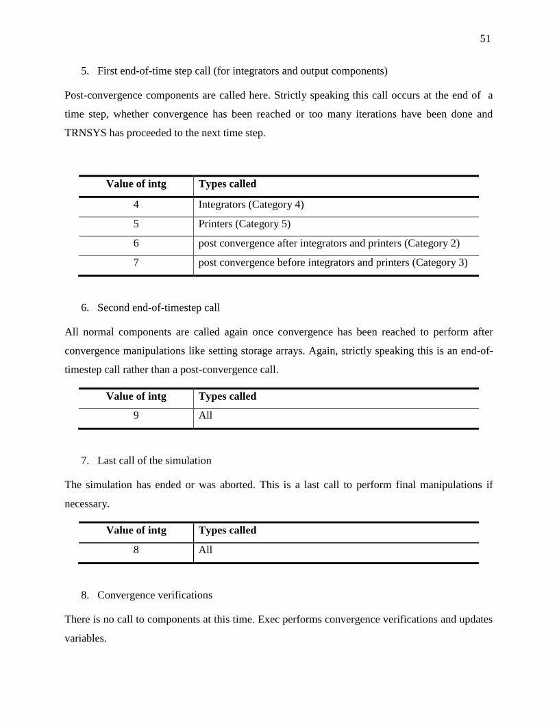
51
5. First end-of-time step call (for integrators and output components)
Post-convergence components are called here. Strictly speaking this call occurs at the end of a
time step, whether convergence has been reached or too many iterations have been done and
TRNSYS has proceeded to the next time step.
Value of intg Types called
4 Integrators (Category 4)
5 Printers (Category 5)
6 post convergence after integrators and printers (Category 2)
7 post convergence before integrators and printers (Category 3)
6. Second end-of-timestep call
All normal components are called again once convergence has been reached to perform after
convergence manipulations like setting storage arrays. Again, strictly speaking this is an end-of-
timestep call rather than a post-convergence call.
Value of intg Types called
9 All
7. Last call of the simulation
The simulation has ended or was aborted. This is a last call to perform final manipulations if
necessary.
Value of intg Types called
8 All
8. Convergence verifications
There is no call to components at this time. Exec performs convergence verifications and updates
variables.

52
Value of intg Types called
10 None
The “Call” arrays
Exec does not call directly the Types but calls an intermediate subroutine Loopex. In order to tell
Loopex which components have to be called, Exec transmits the array “Call”, which includes a
logical variable for each Unit indicating if it has to be called or not. For example Call(3) = true
means that Unit number 3 has to be called.
The Call array is updated by Exec in the simulation depending on the value of ”intg” to call the
right Types at the right time. During initialization, Exec creates 5 models of calling arrays
corresponding to what the Call array should be at specific points in the simulation. The different
calling arrays are presented below:
Table 3-2 “Call” arrays (part 1)
Call1 Array identifying Units which should be called at least once per time step
True: Unit is either time-dependent or has derivative (Category 1)
False: Unit does not need to be called each time step
Call2 Array identifying Units which should be called only at the end of a time step
True: call Unit only at the end of a time step (Category 2)
False: Unit does not need the special "only at the end of time step treatment"

53
Table 3-3 “Call” arrays (part 2)
Call3 Array identifying Units which should be called only at the end of a time step
True: call Unit only at the end of a time step (Category 3)
False: Unit does not need the special "only at the end of time step treatment"
Call4 Array identifying Units which should be called only at the end of a time step
True: call Unit only at the end of a time step (Category 4)
False: Unit does not need the special "only at the end of time step treatment"
Call5 Array identifying Units which should be called only at the end of a time step
True: call Unit only at the end of a time step (Category 5)
False: Unit does not need the special "only at the end of time step treatment"
For each specific moment of the simulation, depending on the value of “intg”, Exec modifies the
Call array by equaling it to one of the models established during initialization.
Loopex
Role
Loopex is the routine that calls the Types and provides them all the information about the time
and the state of the simulation at the moment of the call.
Arguments
Table 3-4 Arguments of Loopex subroutine (part 1)
unit Number of the Unit that should be executed
j jcall loops counter
Time Simulation time
T-Local
Array containing the dependent variables for which derivative are
evaluated.

54
Table 3-5 Arguments of Loopex subroutine (part 2)
DTDT_Local Local table containing the derivatives of T
lastu Last Unit called
intg Determines which Units are called by Exec
Routine that calls Loopex
- Exec
Routines called by Loopex
- Type00
- SetVal
- Trace
Description
The aim of this routine is essentially to call the Types and it also performs some checks,
especially regarding the convergence of the components. It also updates some variables about the
simulation current state: if it is the first time step of the simulation, if convergence has been
reached for the current time step, etc.
3.2.4 Modifications to the code
The addition of the new category of Types has necessitated some modifications to the routines
presented above. New functions and variables have been implemented as well. The changes are
explained here and the modifications to the code can be found in Annex 2.
New variables
Info (9)
The first change brought to the code was the creation of the new category of Types. In order to be
consistent with the TRNSYS management of Types calling, a new value for Info(9) was created.
In addition to the existing values allowed, from 0 to 5, the value 6 was added. Thus

55
implementation of components characterized with Info(9) = 6 is now possible. They include all
Types that need to be called at the same time as standard iterative components (Category 1) but
also right after convergence and before post convergence manipulations.
Call7
An additional array (Call7) which marks Units that have to be called for the new category of
Types was created in Exec. Each value is linked with a Unit and depends entirely of the value of
Info(9) of this Unit.
intg
A new value of “intg” (intg = 11) was created as well and defined in TRNSYS routine. It
corresponds to the moment when all the components have converged (or the maximum number
of iterations has been reached), right before performing the end-of-time step manipulations. It is
the time to call data exchanger components (Info(9) = 6) once again to check the convergence of
the external program.
Info(13)
This variable is a flag indicating that all the Units have converged at the current time step. It is
updated by Exec. Its value is 0 during iterative calls and 1 during post-convergence calls. A new
value has been created for co-simulations. Exec set Info(13) = -2 for the external convergence
checking call that happens between iterative calls and end-of-time step calls.
CosimConvergenceCheckingTime
This logical variable is meant to be checked by Types of the new category. It is set to “true”
when it is the time for exchanger components to check if the other program has converged.
CosimInvocation
The co-simulation process comes with a double level of iterations: internal iterations until
convergence of all the Types and iterations between the two coupled programs. In order to clearly

56
separate the two types of iterations, iterations of the whole system are called “invocations”. This
name was chosen in reference to the middleware that controls the overall convergence and keeps
calling the programs if convergence has not been reached. All these data are counted by the
Harmonizer and relayed to ESP-r and TRNSYS. “CosimInvocation” counts the number of
TRNSYS invocations in a simulation.
CosimInvocationIteration
“CosimInvocationIteration” is the number of iterations for the current invocation. It is different
from the variable “Info(7)”, the number of iterative calls to a specific Unit in the current time
step, which counts the total number of iterations of a component and continue to increment its
value if there are several invocations. On the contrary, “CosimInvocationIteration” is reset after
each new invocation.
CosimNewInvocation
This variable is a logical flag indicating if the ongoing iteration is the first one being done for the
current invocation.
New access functions
In order to make co-simulation variables accessible to other subroutines and especially to Types,
new access functions have been implemented.
- getIsCosimConvergenceCheckingTime() is to be called by a Type to know if the
ongoing call is aimed to check the convergence of the coupled program. The
function sends back the value of “CosimConvergenceCheckingTime”.
- getCosimInvocation() gives the number of invocations “CosimInvocation”.
- getCosimInvocationIteration() gives the number of invocations for the current
invocation “CosimInvocationIteration”.
- getIsCosimNewInvocation() is used to know if the ongoing iteration is the first
iteration of the current invocation. The result is a logical, “CosimNewInvocation”.

57
- SetIterationMode(i) is not a new function but it has been modified to enable the
iteration mode (Info(9))to be set to 6 in the case of components from the new
category of types used in a co-simulation.
TRNSYS
As presented in Figure 3-5, the post-iterations process in the TRNSYS routine was modified. A
new check was added right before proceeding to the end-of-time step calls to the Types. This
check includes a call to Exec with the argument “intg = 11”. It indicates to Exec to call coupling
components only, with the specific task of checking the convergence of the external program.
After the call, TRNSYS checks the value of “CosimConv”. If CosimConv = true, the overall
convergence is reached and TRNSYS calls end-of-time steps components before proceeding to the
next time step. If not, it calls once again all the Types for a new cycle of iterations for the same
time step.

58
Figure 3-5 Modifications to the post iterations process
Iterative calculations
Number of calls > limit number
« warning » message
YES
NO
Post-convergence manipulations
NO
Stable solution
YES
STOPERROR
Beginning of the time step
Convergence or number of calls > limit
number
YES
Restoration of initial variables
NO
STOPNumber of warnings >
limit number
« Warning » message ?
NO
YES
YES
Overall convergence ?
YES
NO
NO

59
Exec
The code of the subroutine Exec was also modified to include a new call to data exchanger
Types. This call is performed between the standard iterative calls and all the post convergence
calls. It is meant to call the components from the new category 6 so that they check the
convergence of the external program. This is the new list of Exec manipulations:
1. Version signing call
2. Initialization call
3. First call of the simulation
4. Iterative call
5. Overall convergence checking call
Value of intg Types called
11 Data exchanger Types (Category 6)
6. First end-of-time step call
7. Second end-of-time step call
8. Last call of the simulation
9. Convergence verifications
Step 5 with calls to Category 6 Types is executed when “intg” is equal to 11. Exec sets the “Call”
array equal to the model of array “Call7”. This new array specific for this point of the simulation
(overall convergence checking time) has been created beforehand during the initialization period.
Changes of other models of calling arrays have also been made. They enable the new category of
Types with Info(9) = 6 to be called with the standard iterative Types from Category 1. Values of
“Call1” linked to data exchanger Types are set to “true” and values from the other models of
calling arrays are set to “false”.

60
Loopex
Modifications done to this subroutine are limited to the addition and update of the new logical
variable “CosimConvergenceCheckingTime”. This variable is set to ”true” by Loopex when
Info(13) = -2. In all the other cases it remains “false”.
3.3 TYPE 130
The Data exchanger component created for running co-simulation with ESP-r is called Type 130.
Its role is to communicate with the Harmonizer and manage the control of internal iterations. In
the exchange of data process, Type 130 works as the complement of the coupling components in
ESP-r.
3.3.1 Generalities in Types coding
Calls structure
Each component routine is organized in 6 parts corresponding to a specific action to be executed,
depending of the kind of call to the Type. The structure is the same for all the categories of Types
but not all the components have specific actions to perform at every call. The organization of a
component code is similar to the one of the subroutine Exec (cf. 3.2.3):
1. Version signing call
2. Initialization call
3. First call of the simulation
4. Standard iteration call
5. End-of-time step call
6. Last call of the simulation
Inputs/Outputs
Communication with other components is realized by a system of inputs and outputs data.
Outputs are data calculated by the Type that can be sent to other components. Inputs are the data

61
coming from other components used by the Type. Their number is defined at the second call to
the Type (Initialization) depending on what the user specified in the deck file.
Code and Proforma
A TRNSYS component requires two files. On one hand the source code (in Fortran or another
programming language) programs all the actions that the Type performs in a simulation: collect
data from the inputs, perform the calculation, set output values, perform additional actions. The
code is either compiled within TRNSYS main DLL or in an external DLL. On the other hand the
proforma can be thought of as the Type “black-box description”. It is used by the Simulation
Studio interface to define the number and the nature of inputs, outputs and parameters of the
Type when the Type is used and configured in a simulation. When a simulation is run from the
Simulation Studio, all the information on component parameters, input-output connections and
simulation controls is written to the TRNSYS input file (deck file) and then read by the kernel.
the proforma must be consistent with the parameters/inputs/outputs description of the component.
3.3.2 Type 130 communication process
Type 130 belongs to the data exchanger Types category and is to be used in a coupled simulation
with the building performance energy modeling software ESP-r. It works as a multiple hydronic
and/or air connector. It receives air and fluids states (temperatures, flow rates) from ESP-r, feeds
them to other components in a TRNSYS simulation, and then sends other air and fluid states back
to the external program. It exchanges data with ESP-r within the time-step. The standard
TRNSYS procedure for connecting components is used to map other Types outputs to Type 130
inputs and Type 130 outputs to the inputs of the other TRNSYS Types as shown in Figure 3-6.
Outputs of Type 130 represent data coming from ESP-r whereas inputs are data sent to ESP-r.
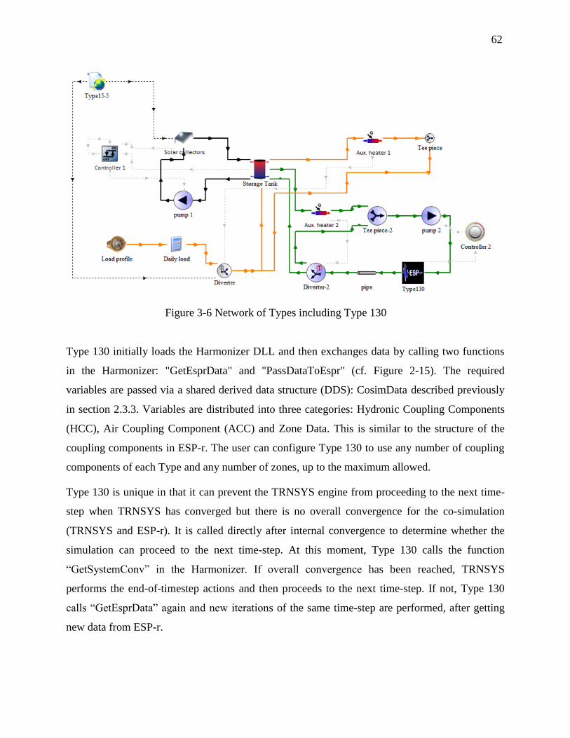
62
Type 130 initially loads the Harmonizer DLL and then exchanges data by calling two functions
in the Harmonizer: "GetEsprData" and "PassDataToEspr" (cf. Figure 2-15). The required
variables are passed via a shared derived data structure (DDS): CosimData described previously
in section 2.3.3. Variables are distributed into three categories: Hydronic Coupling Components
(HCC), Air Coupling Component (ACC) and Zone Data. This is similar to the structure of the
coupling components in ESP-r. The user can configure Type 130 to use any number of coupling
components of each Type and any number of zones, up to the maximum allowed.
Type 130 is unique in that it can prevent the TRNSYS engine from proceeding to the next time-
step when TRNSYS has converged but there is no overall convergence for the co-simulation
(TRNSYS and ESP-r). It is called directly after internal convergence to determine whether the
simulation can proceed to the next time-step. At this moment, Type 130 calls the function
“GetSystemConv” in the Harmonizer. If overall convergence has been reached, TRNSYS
performs the end-of-timestep actions and then proceeds to the next time-step. If not, Type 130
calls “GetEsprData” again and new iterations of the same time-step are performed, after getting
new data from ESP-r.
Figure 3-6 Network of Types including Type 130

63
3.3.3 Type 130 inputs, outputs and parameters
The role of Type 130 is to communicate with ESP-r. Its inputs and outputs are used to exchange
data between a network of TRNSYS Types and ESP-r. Outputs are data coming from ESP-r and
transmitted by Type 130 to other Types. Inputs are variables from other components collected
and sent to ESP-r by Type 130. Figure 3-7 shows the inputs/outputs organization of the
component, as implemented in the source code and the proforma.
Figure 3-7 Inputs and outputs organization
Inputs and outputs are classified in three groups: building zones, HCCs ports and ACCs ports,
and each group contains a subset of data. Information on zones includes heat gains transferred
from mechanical equipment modeled in TRNSYS to a specific zone in ESP-r. This is passed
through an input of Type 130. On the other hand, air temperature and humidity ratio of building
zones can be passed from ESP-r to TRNSYS through outputs of Type 130. ACC and HCC ports
represent respectively data from air flow and fluid flow links. In the case of HCCs, fluid
temperature and flow rate is exchanged for each link. For ACCs, the temperature, the humidity
ratio and the flow rate of the air is transferred in the two ways. Figure 3-8 shows the links
between Type 130 and other components: ESP-r coupling components on the left-hand side and
the other TRNSYS Types on the right-hand side.

64
Figure 3-8 Coupling components connections
Parameters define the number of inputs and outputs of Type 130. This allows the user to
customize the Type and adapt it to the required number of links to ESP-r. There are 7 different
parameters:
1. Mode (standard or test)
2. Number of zones
3. Number of HCC to TRNSYS
4. Number of HCC to ESP-r
5. Number of ACC to TRNSYS
6. Number of ACC to ESP-r
7. Number of forced iterations (only in test mode)
3.3.4 Standard and test modes
The parameter "mode" allows the user to choose between using Type 130 normally and exchange
data with ESP-r (mode = 0) or to use the "test" mode of the type (mode = 1).
If the test mode is selected (mode = 1), Type 130 does not load the Harmonizer DLL. Instead, it
loads a dedicated DLL (Harmonizer_TestMode.dll), which has no link with the Harmonizer
executable program or with ESP-r. "Harmonizer_TestMode" only communicates with Type 130,
and sends back constant output values for a maximum of 2 zones, 2 HCCs and 2 ACCs. This

65
functionality can be used to debug the TRNSYS part of the co-simulation by running the "co-
simulation project" entirely within TRNSYS. Setting the parameter mode to the value 1 in the
proforma brings up a new parameter: NumIterations. It forces the number of iterations for all the
Types connected to Type 130 outputs to be called at least the number of time defined with this
parameter. This can be used to simulate the impact of additional iteration caused by a co-
simulation.
3.3.5 Type 130 code
The complete Type 130 code is given in Annex 3. This part describes the different actions of
Type 130 throughout the calls structure.
1. Version signing call
- Inform the kernel that Type 130 was created under the version 17 of TRNSYS.
2. Initialization call
- Get the number of coupled components from the parameters value and set the
correct number of inputs and outputs.
- Inform the kernel that it is a data exchanger Type
- Load the Harmonizer DLL
- Get pointers to the Harmonizer functions: GetEsprData, PassDataToEspr and
GetSytemConv.
3. First call of the simulation
- Get values from Type 130 inputs and pass them to ESP-r (call to
PassDataToEspr).
- Get data from ESP-r (call to GetEsprData) and set outputs values.
4. First call of a new time step
- Get data from ESP-r (call to GetEsprData) and set Type 130 outputs.

66
5. Standard iteration call
- Keep passing information received from ESP-r at the beginning of the time step to
other TRNSYS components through Type 130 outputs.
6. Overall convergence checking call
- Pass simulation data for ESP-r to the Harmonizer and tell the Harmonizer that
TRNSYS has converged (call to PassDataToEspr).
- Check if ESP-r and overall convergence has been reached (call to
GetCosimConv).
- Tell TRNSYS if overall convergence has been reached: define CosimConv = true
if there is convergence or false in the other case.
- Get new data from ESP-r if there is no overall convergence (call to GetEsprData)
and set Type 130 outputs.
7. Post convergence call
- Type 130 does nothing at this call.
8. Last call of the simulation
- Last call to PassDataToEspr to tell the Harmonizer that simulation is completed in
TRNSYS.
Type 130 updates co-simulation state information for ESP-r and TRNSYS at each time it is
called.
In summary, a list of Type 130 operations compared to a standard TRNSYS Type is presented in
Figure 3-9 Summary of Type 130 calls and operations

67
Figure 3-9 Summary of Type 130 calls and operations

68
CHAPTER 4 DEMONSTRATION AND TESTS
This chapter presents the tests and the results obtained with the co-simulator. From basic data
exchange to complete co-simulation, the testing and debugging phase was a significant part of the
project work. TRNSYS-only tests and the TRNSYS-side of co-simulation tests and debugging
were performed by the author of this MASc thesis with input from the Design Team. Both
programs simulation files for these tests are available on the central repository for ESP-r's source
code (Macdonald & Jost, 2012). Results of demonstration tests are also published in two
conference papers (Beausoleil-morrison et al., 2012; Macdonald, Jost, Beausoleil-morrison,
Mcdowell, & Ferguson, 2012).
4.1 Preliminary tests
A few programmatic checks were performed at the very beginning of the implementation phase
in order to verify the inter DLLs communication design. Compilation and testing of three
simplified DLLS representing ESP-r, TRNSYS and the Harmonizer was realized with success.
The very basic Harmonizer was able to create threads initiating both coupled programs and
exchange data with them. The next tests were executed throughout the project to check if
communication between the three programs worked as expected. The following sections will
describe the preliminary testing procedure for modifications on the TRNSYS side.
4.1.1 External data transfer and iteration control
The main modification to TRNSYS was the addition of a new category of Types and its
capabilities to exchange data with an external DLL and control TRNSYS iterations loops. Prior
to trying to pass and receive data with the real Harmonizer, a test Harmonizer DLL was created.
This DLL was loaded by Type 130 and included the same functions as those that Type 130 is
supposed to call in the real Harmonizer. The functions send data, as simulation variables or flags,
to TRNSYS. Variations of these data helped to test and debug Type 130 and the modified kernel
subroutines. It also proved that the design of the coupling worked: data from another DLL were
conveyed to other TRNSYS components and the new Type was able to prevent TRNSYS from

69
proceeding to the next time-step when the middleware indicated not to do so. This test
Harmonizer DLL, renamed Harmonizer_TestMode, still exists. It has been improved and can be
used by a co-simulator user to test the TRNSYS part of the coupled simulation before using ESP-
r (see the Test mode of Type 130 described above).
4.1.2 Data exchange with ESP-r (Test A)
After the concluding tests with the test middleware, real exchange of data with ESP-r and the
Harmonizer was performed. Both double precision and logical variables were passed back and
forth between the two programs. This step helped to verify that data was passed without being
corrupted.
Data exchange
A first co-simulation test case called Test A was implemented. It does not represent any real
system but each program receives data, modifies it and passes it to the other program. In ESP-r, a
very basic plant system is modeled and sends to TRNSYS a temperature of a fluid associated
with a flow rate. On the TRNSYS side, the project file includes only Type 130, an equation block
and a printer. The equation block receives the temperature and the flow rate coming from ESP-r
and relayed by Type 130. It adds respectively 1 and 2 to the temperature and flow rate values,
and sends the modified variables to Type 130 and ESP-r. Values of exchanged variables were
monitored at different points in the coupling to check that there was no corruption of data at any
step.
Convergence handling
Convergence control by the Harmonizer was also tested. To simulate long cycles of iterations and
control the number of loops, a Type preventing TRNSYS from converging was created. The idea
was to force TRNSYS iterating in a “normal” way, i.e. when inputs of standard Types keep
changing in a simulation. This new Type, known as Type 131, outputs oscillating values for a
fixed number of iterations. If that output is connected to another Type in a TRNSYS network, the
kernel continues calling this Type until its input remains constant. The creation of this Type
allowed defining precisely the number of internal iterations in TRNSYS and helped write the
Harmonizer`s code.

70
4.2 Water based heating system (test B)
This section contains the description of coupled simulation test cases that validates the co-
simulator's ability to simulate a hydronic system.
4.2.1 System tested
The system implemented here modeled a water based heating system for a single-zone building.
As shown in Figure 4-1, the building and a radiator are modeled in ESP-r. The rest of the system
is implemented in TRNSYS. Water supplying the radiator is heated up to 75 °C and circulates at
a flow rate of 500 kg/hr.
Figure 4-1 Schematic of test B system
The HVAC system in TRNSYS comprises: a boiler and pump activated by a controller trying to
maintain a constant room temperature. There are two co-simulation variants:
B1 where an on/off controller is used to control the flow rate of a constant temperature
stream of water

71
B2 where an on/off controller is used to control the temperature of a constant flow rate of
water
In both test cases the dead band of the controller is 2°C. Since the heating set-point is 20°C, the
system is activated by the controller when temperature of the air in the zone decreases below
19°C and is turned off when the air temperature is higher than 21°C.
4.2.2 ESP-r
The building modeled in ESP-r is based upon BESTEST case 600 (Judkoff & Neymark, 1995). It
uses a plant network consisting of a sending and receiving HCC (Hydronic Coupling
Component) and a radiator in ESP-r.
Figure 4-2 Overview and front view of BESTEST case 600 building
4.2.3 Simulation using TRNSYS only
In order to compare results obtained from the co-simulation, a test case implemented only in
TRNSYS was created. The TRNSYS part already existing in the coupled simulation is the same
here. As presented in Figure 4-3, the “red” loop with the pump, the heater and the controller is
unchanged in comparison to the co-simulation project. Type 130 has been replaced by
components that were implemented previously in ESP-r: the building and the radiator. A weather
data reader Type loading the same weather file as ESP-r in the co-simulation case is also added
here.

72
Figure 4-3 TRNSYS only simulation for Test B
The radiator model implemented for this simulation is based on the following equation
(ASHRAE, 2008):
Where:
Table 4-1 Radiator model parameters
Heating capacity W
Constant determined by test
Arithmetic average of the entering and leaving water temperature °C
Room air temperature °C
Exponent for cast-iron radiators 1.2
The room air temperature is known at every time step. To define the temperature of water exiting
the radiator and energy injected into the zone, an energy balance on the radiator is performed:

73
Where:
Table 4-2 Description of radiator governing equation variables
Water mass flow rate kg/hr
Water specific heat 4.19 kJ/kg.K
Entering water temperature °C
Leaving water temperature °C
The building is modeled by the multi-zone building component Type56, which was configured to
model BESTEST Case 600.
4.2.4 Results analysis
Results obtained from co-simulation prove that control of the system by TRNSYS based on data
transmitted by ESP-r is effective. The temperature of the thermal zone is maintained at a value of
20 °C. Moreover, a comparison of results from a co-simulation with a TRNSYS only simulation
(Figure 4-4) shows that the evolution of zone air temperature is similar.
Figure 4-4 Comparison of zone air temperature for two winter days
0
10
20
30
40
50
60
0 5 10 15 20 25 30 35 40 45
Zon
e te
mp
erat
ure
(°C
)
Time (hr)
Co-simulation
TRNSYS only

74
The graph represents the temperature of the air in the building for a sunny and a cloudy winter
days. Since the building has a largely glazed façade oriented towards the South and there is no
cooling system, high temperatures are reached in the afternoon of day 1. The rest of the time
there is no solar contribution to maintain the temperature of the zone higher than 20 °C, therefore
the heating system is ON. Temperatures coming from the two simulations are close, yet we can
notice some differences. The afternoon peak is higher in the case of the co-simulation. The same
effect can be observed with variations of temperature around the set-point, which are greater with
results obtained with the co-simulation case. These variations are explained by the fact that the
radiator and building models are not the same in the two programs, even if an effort was made to
reconcile their parameters. The main difference is that the model of radiator is transient in ESP-r
whereas a steady state model with no mass has been implemented in TRNSYS.
The two following graphs presented in Figure 4-5 show more in details that the whole system is
working properly for a coupled simulation. On the right side, temperature of the zone (blue) and
water flow rate (green) are plotted for the B1 simulation. The temperature of the water provided
to the radiator is constant, but the flow rate is variable. The graph shows that the pump is turned
OFF as expected when the temperature of the air is higher than 21°C and switched ON when the
temperature is under 19°C. The mechanical system controlled in TRNSYS is able to react to and
control a temperature of a thermal zone implemented in ESP-r. It can be noted that the
temperature of the air continues to rise after the flow of the water to the radiator is stopped. This
is explained by the capacity of the water in the radiator. Even if there is no more hot water
supplied to the radiator, the water inside the radiator is still warm enough to heat the air for a
certain time.
Figure 4-5 Evolution of the zone air temperature for the two test cases B1 (right) and B2 (left)

75
The second graph of Figure 4-5 shows results from the B2 simulation, where the flow rate is kept
constant but the temperature of the water provided to the radiator changes. The air temperature,
(blue) and the water temperature at the inlet of the radiator (red) are represented. As long as the
temperature of the zone remains lower than 21 °C, the boiler heats the water up to a maximal
temperature of 75 °C. Then the temperature of the air decreases slowly, and when it goes under
19 °C, the water is heated again.
Results from the previous simulations are not optimized. The control of the temperature works
but the amplitude between the highest temperatures (around 23 °C) and the lowest ones (around
19 °C) is large. The lack of accuracy in tracking the setpoint comes from the ON/OFF nature of
the simulated control system. Another simulation was created with a PID controller for the water
flow rate. Figure 4-6 shows that the temperature curve is smoother in this case and the
temperature of the zone is close to 20 °C.
Figure 4-6 Evolution of the zone air temperature and water flow rate with a PID controller
4.3 Air based heating system and humidity transfer (test D)
The tests presented here were created in order to check the correct transfer of humidity in a co-
simulation. Two cases of studies were developed. The first modeled is a single zone building
with constant boundary conditions without any source of humidity. Another model was tested
then with the same building but this time with a constant internal source of humidity. In both
cases a ventilation system adds fresh air at a constant humidity rate and constant flow rate.

76
4.3.1 No humidity source
System
Figure 4-7 illustrates the system implemented for this test. A simple isolated thermal zone
modeled in ESP-r is humidified by a ventilation system in TRNSYS.
Figure 4-7 Schematic of test D system without humidity source
Settings:
Table 4-3 Settings of Test D without humidity source
Air flow rate
Water flow rate
Humidity ratio of supplied air
The building has constant boundary conditions. The climate file used in ESP-r has zero solar
radiation, an ambient temperature of 20 °C and a relative humidity of 50 %.

77
Results
The test shows the correct results for transient conditions as well as for steady state. In Figure
4-8, we can observe the evolution of the humidity ratio of the air in the zone. The supplied air
contains a constant quantity of humidity. As predicted, the value of humidity ratio of the zone
converges to the one of humidity ratio of the supplied air.
Figure 4-8 - Transient state humidity ratios
The test is then continued to a week. Differences between the humidity ratio of the air injected in
the zone and the air leaving the zone are compared and represented in Figure 4-9. The graph
shows that the two humidity ratios are similar. The maximum difference between the two values
is less than 10-7
and can be attributed to rounding errors inherent to computers.
Figure 4-9 - Differences between HR send to the zone and HR of the zone
0.00E+00
5.00E-04
1.00E-03
1.50E-03
2.00E-03
2.50E-03
3.00E-03
3.50E-03
TIME(hr)
0.15 0.32 0.48 0.65 0.82 0.98 1.15 1.32 1.48 1.65 1.82 1.98
HR to zone
HRzone
0
1E-08
2E-08
3E-08
4E-08
5E-08
6E-08
7E-08
8E-08
error

78
4.3.2 Constant humidity source
System
The building is the same as in the first test case. The humidifying system is simplified to a
system that sends air at a constant absolute humidity level without changing the temperature
of the air (i.e. the supply air temperature is the temperature of the thermal zone). A source of
humidity has been added inside the thermal zone (latent heat gain) for this second simulation.
Figure 4-10 Schematic of test D system with constant humidity source
Settings:
Table 4-4 Settings of Test D with Humidity source
Air flow rate
Humidity ratio of supplied air
Latent energy source
The building and the climate file are the same as those used in the first case.

79
Results
For this test a simulation of one week (168 hours) was performed. Results obtained at the end of
the simulation are presented below:
Temperature of the air in the zone (DB): T168 = 16.3 °C
Humidity ratio of the air in the zone: HRzone 168 = 0.00308537 kg/kg
Verification of the value of the amount of humidity in the zone with a mass balance:
Where: is the mass of water added in the zone in kg of water/hr
is the humidity ratio of the air leaving the zone
The heat gain in ESP-r is purely latent. We can assume that it corresponds to adding a given
flowrate of saturated steam at the room temperature, and we have:
Where: is the enthalpy of the water added in the zone in kJ/kg of water
The enthalpy of the added water is:
and:
By solving the mass balance, we find:
kg/kg
We find the same value as the one from the co-simulation so humidity transfer between the two
programs can be validated.

80
The error/difference between the value calculated and the one obtained numerically is:
δ = 2.95 E-08. kg/kg
(or a relative error of less than 0.001 %)
4.4 House serviced by a DHW/space heating solar combi-system (test C)
The co-simulation tested here includes a simple house (modeled in ESP-r) and a solar combi-
system (modeled in TRNSYS) used for space heating and domestic hot water production. The
models and obtained results are described below.
The TRNSYS part of the combisystem model was developed and configured by the author of this
MASc thesis with input from the Design Team. The building model in ESP-r was developed and
implemented by the Carleton University team. Debugging, model tuning and results
interpretation were a team effort. This test was a project deliverable requested and the following
section is part of a report submitted to Natural Resources Canada. The lead author for the
deliverable was the author of this MASc Thesis, who also created the TRNSYS part of the co-
simulation model.
4.4.1 System tested
The simulated system includes a 3-zone house and a solar combi-system used to meet the space
heating load of the house and to provide domestic hot water. A schematic of the whole system is
shown in Figure 4-11, with the mechanical system modeled in TRNSYS and the building in
ESP-r.
The house is modeled as a 3-zone building where the temperature of the main floor is kept
at 20 °C by the solar combi-system. This exercise focuses on solar heating, so cooling and natural
ventilation are not modeled. This results in very high zone temperatures on sunny days,
particularly during the summer.
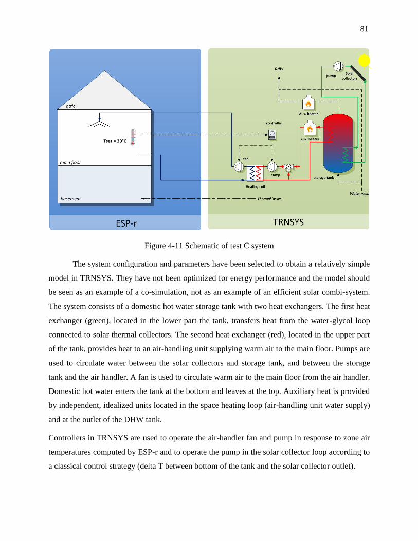
81
Figure 4-11 Schematic of test C system
The system configuration and parameters have been selected to obtain a relatively simple
model in TRNSYS. They have not been optimized for energy performance and the model should
be seen as an example of a co-simulation, not as an example of an efficient solar combi-system.
The system consists of a domestic hot water storage tank with two heat exchangers. The first heat
exchanger (green), located in the lower part the tank, transfers heat from the water-glycol loop
connected to solar thermal collectors. The second heat exchanger (red), located in the upper part
of the tank, provides heat to an air-handling unit supplying warm air to the main floor. Pumps are
used to circulate water between the solar collectors and storage tank, and between the storage
tank and the air handler. A fan is used to circulate warm air to the main floor from the air handler.
Domestic hot water enters the tank at the bottom and leaves at the top. Auxiliary heat is provided
by independent, idealized units located in the space heating loop (air-handling unit water supply)
and at the outlet of the DHW tank.
Controllers in TRNSYS are used to operate the air-handler fan and pump in response to zone air
temperatures computed by ESP-r and to operate the pump in the solar collector loop according to
a classical control strategy (delta T between bottom of the tank and the solar collector outlet).

82
4.4.2 TRNSYS
Figure 4-12 shows the solar combi-system modeled in TRNSYS. The system is made up of four
circuits: a solar circuit (green); a domestic hot water circuit (orange); an air loop (blue) and a
water heating circuit (red).
Figure 4-12 TRNSYS simulation for Test C
Solar collectors circuit
The collectors are oriented to the south (azimuth angle = 0°) with a slope of 45°. The parameters
used to describe the collectors are:
Table 4-5 Parameters of solar collectors
Tested flow rate 75 kg/hr.m2
Intercept efficiency 0.811 -
Efficiency slope 2.710 W/(m2.K)
Efficiency curvature 0.010 W/(m2.K
2)
1st order IAM 0.072 -
2nd
order IAM 0 -

83
The heat transfer fluid is a mix of water and glycol, with a specific heat of 3.6 kJ/kgK, and
circulated at a flow rate of 200 kg/hr.
The stratified storage tank used to store the solar energy encompasses two immersed heat
exchangers. Thermal losses (in kWh/day) from the storage tank are calculated using equation 12:
Where V = the volume of the tank in liters. This equation allows thermal losses to be adapted in a
simple way when the tank volume is varied.
Pumps are turned on and off by a differential controller which compares the temperatures at the
output of the solar collectors and with those in the tank, to prevent cooling the stored water when
temperature in the solar circuit is lower than the temperature of the water in the tank.
Domestic hot water circuit (DHW)
A daily load profile was used to simulate the consumption of domestic hot water. Figure 4-13
illustrates the hot water demand profile.
Figure 4-13 DHW load profile
2 Category B of storage tank for a difference of temperature of 45°C with the outside of the tank , EU standard EN
15332 : 2007
0
5
10
15
20
25
30
35
40
45
0 1 2 3 4 5 6 7 8 9 10 11 12 13 14 15 16 17 18 19 20 21 22 23 24
flow rate (kg/hr)
time (hr)

84
Domestic hot water is supplied at 60°C. If the tank outlet temperature is lower than this, the
auxiliary heater provides additional heat to reach the set point. If the tank outlet temperature is
higher than 60 °C, the auxiliary heater is not used. A thermostatic valve brings the DHW supply
temperature to 45 °C for distribution in the house (that thermostatic valve is modeled as a
controlled diverter and a tee in TRNSYS).
Heating circuits
The temperature set point for water supplied to the air handler is 60 °C. An auxiliary heater is
used to reach the set point when required. If the temperature of the tank is higher than 60 °C, a
three way valve is used to partially bypass the heat exchanger in the tank and recirculate water
towards the air handler.
An on/off controller activates the pump depending on the temperature of the zone. The flow rate
of the pump is 400 kg/hr.
A length of 10 meters of piping with a diameter of 0.02 m were also modeled for this loop. Their
heat losses and those from the tank are all injected in the basement zone in the building.
On the load side of the water-air heat exchanger, warm air is circulated to the main floor. An
ON/OFF controller is used to actuate the fan providing a flow rate of 1200 kg/hr of warm air
when the temperature of the main floor falls below 20 °C. Both sides of the heating coil, source
and load, are activated simultaneously by this controller. The dead band is 2 °C centered on
20 °C.
Type 130
For this demonstration Type 130 was configured with three zones (basement (zone 1), main floor
(zone 2), and attic (zone3)), One air coupling port (ACCToTrnsys and ACCToEspr) and no
hydronic coupling ports. Figure 4-14 represents the inputs/outputs connections of the Type.

85
Figure 4-14 Type 130 connections
4.4.3 ESP-r
Figure 4-15 illustrates the model of the three zone building in ESP-r. The model is taken from the
CCHT house (CCHT 2008) which comprises three thermal zones: basement; main floor and
second floor; and attic space. The original model included an attached garage which was not
modeled for this example.
Figure 4-15 Zone house model in ESP-r

86
4.4.4 Coupling settings
The link between the two programs is maintained by the TRNSYS data exchange component,
Type 130 and by two air-based coupling components, ACC_toESPr (responsible for data sent
from TRNSYS to ESP-r) and ACC_toTrnsys (responsible for sending data from ESP-r to
TRNSYS). Figure 4-16 shows how these components are connected with the whole simulation.
Figure 4-16 Connections at the interface between the two programs
The common simulation parameters (time step and weather data) in both programs were specified
as follows:
Table 4-6 Co-simulation parameters for Test C
Duration of the simulation 1 year
Length of the startup period (ESP-r): 1 day
Length of the startup period (ESP-r): 1 minute
Weather data file Toronto (CWEC)

87
4.4.5 Results analysis
Convergence
The co-simulation runs until the end of the period (1 year) without any convergence issues; none
of the TRNSYS components fail to converge at any time-step and ESP-r and the harmonizer
attain convergence at every time-step. The number of invocations and iterations required to reach
convergence are summarized below. Figure 4-17 illustrates the iterations per time-step over a
section of the simulation period. As the plant network in ESP-r is very basic, and ESP-r does not
perform iterations between the plant domain and the building domain, so the number of ESP-r
iterations is equal to the number of invocations.
Table 4-7 Combi-system co-simulation results (annual simulation)
Simulation running time 16 min
Total number of invocations 1,069,150
Average number of invocations per time-step 2.04
Total number of ESP-r iterations 1,069,150
Total number of TRNSYS iterations 3,150,191
Average number of ESP-r iterations per time-step 2.04
Average number of TRNSYS iterations per time-step 6.01

88
Figure 4-17 Number of iterations per time-step
Energy balances
Figure 4-18 Energy transfers in the system

89
The following energy balances were performed to verify the results obtained from co-simulation.
The data was derived from an annual simulation with a solar collector area of 10 m2 and a tank
size of 0.5 m3. Figure 4-18 shows the energy quantities used in the thermal balance:
Table 4-8 Description of energy transfers
Q1 Energy from solar collectors entering
the storage tank
Q7
Energy from the auxiliary heater
added to the water space heating loop
Q2 Energy transferred from the tank to
the water space heating loop
Q8
Thermal energy losses of the pipes
Q3 Energy transferred from the tank to
the domestic hot water circuit
Q9
Energy transferred from water space
heating loop to the air
Q4 Thermal energy losses of the storage
tank
Q10
Energy provided to the main floor
zone
Q5 Energy stored in the tank Q11
Total thermal energy losses of the
equipment
Q6 Energy from the auxiliary heater
added to the domestic hot water
circuit
Q12
Energy entering the basement zone
from the equipment thermal energy
losses
The purpose of each energy balance is to verify that the amount of energy entering the system is
equal to the energy exiting and stored in the system. The error in the energy balance is calculated
as follows:
∑ ∑
∑ ∑
With: ∑ the sum of energy entering the system
∑ the sum of energy exiting and stored by the system
Four energy balances were performed, one for each of the following energy systems: the storage
tank; the water side of the space heating loop; the air side of the space heating loop; and for the

90
plant thermal losses. Only TRNSYS values are used in the storage tank and water space heating
circuit. The air side of the space heating circuit and the plant thermal loss energy balances
demonstrate the data exchange between the programs.
- Storage tank
Q1 = Q2 + Q3 + Q4 + Q5
Q1 = 3 891 kWh
Q2 + Q3 + Q4 + Q5= 1 335 + 2 528 + 11 + 14 = 3 887 kWh
- Space heating loop (water)
Q2 + Q7 = Q8 + Q9
Q2 + Q7 = 1 335 + 16 233 = 17 568 kWh
Q8 + Q9 = 68 + 17 500 = 17 568 kWh
- Space heating loop (air)
Q9 = Q10
Q9 = 17 500 kWh
Q10 = 17 419 kWh
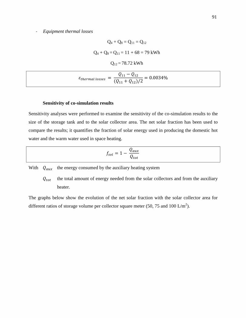
91
- Equipment thermal losses
Q4 + Q8 = Q11 = Q12
Q4 + Q8 = Q11 = 11 + 68 = 79 kWh
Q12 = 78.72 kWh
Sensitivity of co-simulation results
Sensitivity analyses were performed to examine the sensitivity of the co-simulation results to the
size of the storage tank and to the solar collector area. The net solar fraction has been used to
compare the results; it quantifies the fraction of solar energy used in producing the domestic hot
water and the warm water used in space heating.
With the energy consumed by the auxiliary heating system
the total amount of energy needed from the solar collectors and from the auxiliary
heater.
The graphs below show the evolution of the net solar fraction with the solar collector area for
different ratios of storage volume per collector square meter (50, 75 and 100 L/m2).

92
Figure 4-19 Space heating solar fraction
Figure 4-19 illustrates the solar fraction contributing to space heating and shows that solar energy
contributes only modestly to the space heating of the house. Without a large area of collectors,
the energy from the solar collectors used in heating the zone remains small. The system could be
optimized to increase the solar fraction but the results show that the system behaves as expected.
Increasing the number of collectors and the storage volume increases the solar energy collected
and stored and thus reduces the auxiliary heating energy.
Figure 4-20 Domestic hot water solar fraction
6%
11%
16%
21%
26%
31%
36%
41%
46%
10 20 30 40 50
Collectors area (m2)
Heating solar fraction
50 L/m2
75 L/m2
100L/m2
86%
87%
88%
89%
90%
91%
92%
10 20 30 40 50
Collectors area (m2)
DHW solar fraction
50 L/m2
75 L/m2
100L/m2

93
The same trend can be seen in the results for the solar fraction contributing to the domestic hot
water (DHW) heating, as illustrated in Figure 4-20. With the DHW the solar fraction is higher
and energy collected from the sun is almost enough to heat the water on its own. Even with a 10
m2 collector area, auxiliary heating required rarely exceeds 14 %.
Figure 4-21 shows the global solar fraction of the combi-system.
Figure 4-21 System total solar fraction
The results presented in this section demonstrate that the runtime coupling functions as intended
and that it provides a useful tool in the analysis of NZEBs.
The coupling has enabled the following data exchanges:
- flow, temperature and humidity data computed by a network of TRNSYS types onto an
ESP-r plant network (in this case air exiting the air handling unit and entering the
building)
- flow and temperature data computed by an ESP-r plant network as boundary conditions
on a network of TRNSYS types (in this case return air from the building to the air
handling unit)
- temperature and humidity conditions within the building as boundary conditions on the
TRNSYS network (in this case environment conditions for tank and piping)
17%
22%
27%
32%
37%
42%
47%
52%
57%
10 20 30 40 50
Collectors area (m2)
Total solar fraction
50 L/m2
75 L/m2
100L/m2

94
- heat transfers from TRNSYS networks as boundary conditions (including internal gains)
within ESP-r’s building envelope model (in this case thermal losses from the tank and
pipes injected into the basement)
The simulation converges and energy balances have been verified. The results obtained by co-
simulation correspond to the trends that were expected for the modeled solar combi-system and
house.

95
CHAPTER 5 USING THE ESP-R / TRNSYS CO-SIMULATOR
This last chapter is describing how to perform co-simulations from a user perspective. The
creation of the input file for the coupled programs and for the Harmonizer will be presented.
Then, we will show how to run a co-simulation and how to collect the results.
This chapter essentially contains the same information as the “getting started” user guide that is
distributed with the Harmonizer as part of the ESP-r and TRNSYS packages. The TRNSYS-
specific instructions were written by the author of this thesis, while the instruction specific to
ESP-r were authored by the Carleton University team.
5.1 Generalities
One of the main objectives in the design of the co-simulator was to minimize modifications to the
existing programs. In comparison to a standard simulation with only one program, the same
external simulation files are used in a co-simulation. Users who are already familiar with both
programs should have no problems following the procedure for coupled simulations. Figure 5-1
lists the external files involved in a co-simulation.
Figure 5-1 Co-simulator's input and output files
On the ESP-r side, an input file with the “.cfg” standard ESP-r input file format is required, as
well as the associated directories and files describing the entire ESP-r project. The user can either
create the model from the Project Manager interface or by editing the input file. The same
principle applies to TRNSYS, where the deck file includes the complete model description,
HARMONIZERESP-r TRNSYS
xxx.harxxx.harxxx.cfgxxx.cfg xxx.dckxxx.dck
xxx.csvxxx.csv xxx.txtxxx.txt
Input filesInput files
Output filesOutput files

96
whether performing a TRNSYS-only or a coupled simulation. Output files can be generated by
both programs as they are for standard ("one-program") simulations. A standard “.csv” output file
can be defined and configured in ESP-r. In TRNSYS, all standard output components can be used
(printers, simulation summaries, etc.). A new, co-simulation specific input file is required for the
Harmonizer. This Harmonizer input file specifies co-simulation parameters.
5.2 Harmonizer input file
Figure 5-2 Harmonizer input file
The Harmonizer input file indicates to the Harmonizer launcher where to find every program’s
DLL and some information about a specific co-simulation. The first lines specify the path to
TRNSYS, ESP-r and the Harmonizer DLL. This ensures that co-simulations can be performed
with both programs installed in user-specific locations, as long as both programs were installed
properly and that the main ESP-r and TRNSYS DLL’s are capable of finding their own

97
secondary files. Then, paths to the ESP-r (.cfg) and TRNSYS (.dck) model files are specified.
Finally, four convergence criteria can be specified by the user: temperature, fluid flow rate,
moisture flow rate and the maximum number of invocations per time-step. The temperature
change criterion is an absolute value in °C, while the two flow rate change criteria are relative
values in % (that revert to absolute change if the flowrate is close to 0). That last line is optional.
If it is not present, default values are used: 0.001°C for the temperature, 0.05% for flow rates and
the number of invocations is limited to 20 per time step.
An example of Harmonizer input file with user-specified convergence criteria is given below:
2.0 # File version number
# Path to Harmonizer.dll
C:\Harmonizer\Harmonizer.dll
# Path to bps.dll
C:\ESRU\Esp-r\bin\bps.dll
# Path to TRNDll.dll
C:\Trnsys17\Exe\TRNDll.dll
#Command line to be used for the bps simulation
bps -file C:\path_to_ESP-r_model\cfg\cfgfile.cfg -mode text -p test silent
# Path to TRNSYS deck file to be used in the co-simulation
C:\Path_to_deck_file\deck_file_name.dck
# Convergence criteria: Temperature, Flow, Moisture flow, Max No of invocations
0.001, 0.05, 0.05, 20
5.3 ESP-r model
An ESP-r co-simulation model is created as a traditional model using ESP-r only. The only
difference is the addition of the coupling components in the plant domain. The different steps to
create a model for a co-simulation are detailed below. It is assumed that the building is already
modeled and only the configuration of the coupling components will be described.

98
Figure 5-3 ESP-r input file
1. Create a plant system
Starting from the Project Manager main window:
- Select option m: /browse/edit/simulate
- Select option d: plant & systems
- Select option b: Explicit (plant network)
- Create a plant network (yes)
- Proceed with network description (yes)
- Select database plantc.db1 (should be default)
2. Add coupling components
In the plant definition window:

99
- Select option d: Components
- Add component
- Select option d: Solar and others
- Select the components you require and give them a meaningful name. The index of the
component is used if you wish to change the order in which components are linked to
TRNSYS. Figure 5-4 shows the addition of two HCC and two ACC (sending and
receiving) components together with a radiator.
Figure 5-4 Example of a plant system including coupling components
3. Configure the connections
In the plant definition window:
- Select option e: Connections and add the required connections to connect the
components.

100
There are two different cases depending on the nature of the exchanged fluid. If the coupling
components are Hydronic Coupling Components, they have to be connected to at least one other
component of the plant. In the case of Air Coupling Components, they need to be linked to a
thermal zone. Schematics of these connections are presented in Figure 5-5. In both cases, a
connection has to be defined between the two Coupling Components of one fluid connection to
TRNSYS (sending and receiving).
radiator
HCC_to_ESP-r
HCC_to_TRNSYS
ACC_to_ESP-r
ACC_to_TRNSYS
Zone
Figure 5-5 Coupling components connections: HCC on the left and ACC on the right
(Macdonald, 2012)
The corresponding connections to the previous example of HCC and ACC in the Project manager
is shown in Figure 5-6.
Figure 5-6 Example of connections for ACCs (blue) and HCCs (red)

101
4. Define the simulation preset
The preset is what is used to define the simulation parameters. From the Browse/Edit/Simulate
menu:
- Select option r: simulation
- Select option a: simulation presets
The start-up period, simulation dates and time-steps are defined here. The co-simulation Design
Team recommends that ESP-r plant time-step should always be equal the zone time-step, and the
results save level should be set to 5 to get the xml output.
5.4 TRNSYS model
5.4.1 Creation of TRNSYS input file
Figure 5-7 TRNSYS input file

102
1. Create the system network
The example below (Figure 5-8) shows the system network for a combi-system providing heat to
a building through the air-handling unit (heat exchanger in that model).
Figure 5-8 TRNSYS network of Types
2. Add Type 130 to the project
Type 130 is added to the project by selecting the component in the list of Types and dragging it
to the Assembly window.

103
Figure 5-9 Addition of Type 130 to the network of Types
3. Define the number of zones, ACCs, and HCCs components in Type 130 parameters
Figure 5-10 Type 130 parameters settings
ACCs, HCCs and zones must be defined in the same order as in ESP-r. This particular example
uses one ACC To TRNSYS (inlet of the fan) and one ACC To ESP-r (outlet of the secondary
side of the heat exchanger).

104
4. Connect Type 130 inputs and outputs to the other components
The connections between Type 130 and the other components are presented in red in Figure 5-11.
The ACC To TRNSYS data (flowrate, temperature and humidity available as outputs from Type
130) is connected to the matching fan inputs. Outlet conditions from the heat exchanger are
connected to the ACC to Esp-r (Type 130 inputs). The basement zone temperature calculated by
Esp-r (available as an output of Type 130) is connected to the storage tank environment
temperature. The main floor temperature is connected to the thermostat. Finally, thermal losses
from the tank and pipes are connected to the input of Type 130 representing casual gains for the
basement zone.
Figure 5-11 TRNSYS network of Types with Type 130
5. Define the same time-step and simulation start and stop time
These parameters are defined in the control card windows. They have to be the same as those
defined in ESP_r. Special care must be taken to take the ESP-r startup period into account (refer
to section 5.5.1 for more details).

105
Figure 5-12 Simulation parameters
6. Create the .dck file and save the Studio file (.tpf)
The deck file is created by selecting Calculate/Create input file or by clicking on the pen icon in
the Simulation Studio window. Unlike the deck file, the Studio file (.tpf) is not necessary to run
the co-simulation but it is worth saving it to be able to re-open it later and modify it in the
Simulation Studio.

106
Figure 5-13 Creation of TRNSYS input file
5.4.2 Type 130 Test mode
Before running a co-simulation with ESP-r, it is possible to test and debug the TRNSYS part by
activating the test mode of Type 130. This enables exchanging data with a test-mode version of
the Harmonizer DLL. This test-mode DLL sends constant values to a maximum of 2 zones, 2
HCCs and 2 ACCs. Results obtained using the test mode are not realistic but can be useful in
testing the system created and identifying errors on the TRNSYS-side of the simulation more
easily.
Another functionality allowed by this mode is to set the number of minimum iterations of
components linked to the Harmonizer. A new parameter appears in Type 130 proforma:
NumIterations which defines this number of forced iterations. This was developed in order to
simulate the action of the real Harmonizer which may invoke some types many times per time
step. Again, this capability can be used to debug the TRNSYS-side of the simulation (e.g. user-
created components) to make sure the extra iterations that will likely result from the co-
simulation do not have undesired side effects.

107
1. Define the parameter Mode = 1
2. Choose the number of forced iterations (the minimum is one, which means no forced
iterations). All types connected to a Type 130 output will be forced to iterate this number of
times.
3. Save the project (.tpf)
4. Run the simulation directly from the Studio
5. Constant values sent by Type 130 in test mode:
Table 5-1 Constant values sent by Type 130 in test mode
Zone 1 Temperature 21 °C
Humidity Ratio 0.006 -
Zone 2 Temperature 22 °C
Humidity Ratio 0.007 -
HCC 1 Temperature 31 °C
Flow-rate 101 kg/hr
HCC 1 Temperature 32 °C
Flow-rate 102 kg/hr
ACC 1
Temperature 41 °C
Humidity Ratio 0.0004975 -
Flow-rate 201 kg/hr
ACC 2
Temperature 42 °C
Humidity Ratio 0.0004950 -
Flow-rate 202 kg/hr
5.4.3 Note about controllers
Running a co-simulation increases the total number of iterations per time-step in TRNSYS due to
the multiple invocations. It is advised to increase the default value of the maximal number of
iteration allowed in the deck file. Indeed, the initial value fits with a simulation using TRNSYS
only. Modifying the parameter prevents the simulation to stop with a convergence error message
while the actual reason is that co-simulation necessitates more iterations than a standard
simulation.

108
Some Types such as controller Type 2 (ON/OFF controller, standard library) and a series of
similar controllers in the TESS libraries (aquastat, humidistat, multi-stage controller, etc.) may
be affected by a large number of iteration in a time-step. These Types sense a variable (e.g:
temperature, humidity, etc,) and depending on its value send a corresponding control signal. At
each iteration, the output of the controller may change if the value of the sensed variable is
different. In order to prevent non convergence issues the number of oscillations for the controller
within a time step is limited. These types either count the number of times they were called or the
number of oscillations (discrete change in the output signal) within a time step, and if that
number exceeds a threshold set by the user they “stick” to their value. Co-simulation may
include a significant number of iterations resulting from successive invocations and not from
oscillations within TRNSYS. In such a case, after few (or even one) invocations these Types
would “stick” to their values before even performing one oscillation in a given invocation.
To prevent this type of issue, new functions that inform Types about the number of invocations
and the number of iteration per invocation were created. They are presented above in section
3.2.4. It is recommended to modify the source code of Types that use the principle of “sticking”
to a value after a given number of iterations or oscillations. Instead of basing the oscillations
limitation on the total number of iterations or the total number of oscillations within a time step,
they should reset the number of counted iterations or oscillations to zero at each new invocation.
An example of changes needed for Type 2 is given in ANNEX 2.
5.5 Co-simulation
Once the TRNSYS and ESP-r model files have been defined, the co-simulation is ready to run.
The following instructions describe how to proceed to launch a co-simulation and recover the
results.

109
5.5.1 Running a co-simulation
It is important to first ensure that the simulation periods in TRNSYS and ESP-r are the same (i.e.
same start and end days and same number of time-steps per hour). If a climate file is used in
TRNSYS, users should also make sure it matches the weather data used in ESP-r.
Unlike TRNSYS, ESP-r begins simulating with a specified startup period and this needs to be
calculated when defining the TRNSYS start time. As an example, an hourly simulation from start
= 0 to stop = 8760 in TRNSYS would match a simulation from the 2nd
of January to the 31st of
December in ESP-r with a one-day startup period. If the ESP-r simulation starts on the 1st of
January, the start-up period in ESP-r actually represents the last hours or days of the previous
year. In TRNSYS, a start time = 0 always represents January first at 0:00 AM, and negative time
values are not possible. The solution in such a case is to start the TRNSYS simulation at a time a
few hours or day before the end of the first year, and finish it after the second year. For an annual
ESP-r simulation starting on January 1st with a 14 day start-up period, the TRNSYS start time
would be 8424 and the stop time 17520.
The co-simulation can be launched from the Windows command prompt, a MinGW or Cygwin
window. For the three cases, the Harmonizer is invoked from the directory containing the
Harmonizer input file by entering the absolute path to the Harmonizer executable program
following by the name of the Harmonizer input file.
E.g. : C:/Harmonizer-install-directory/harmonizer.exe my_model.har

110
5.5.2 Results recovery
Figure 5-14 Co-simulation output files
The procedure to specify output files in ESP-r and TRNSYS is the same within each program as
for “one-program” simulations.
ESP-r
ESP-r will produce a .csv file (in the cfg directory) with data as specified in the input.xml file
which should be located in the /cfg directory. Two example input.xml files are provided here.
The first output specific data only, including zone air point temperatures and humidities as well
as all the data passed between ESP-r and TRNSYS.
<?xml version="1.0" encoding="UTF-8"?>
<configuration>
<apply_style_sheet>false</apply_style_sheet>
<dump_all_data>false</dump_all_data>
<enable_xml_wildcards>true</enable_xml_wildcards>
<hierarchy>flat</hierarchy>
<link_style_sheet>false</link_style_sheet>

111
<output_dictionary>true</output_dictionary>
<report_startup_period_data>false</report_startup_period_data>
<step_variable>building/time_step</step_variable>
<step_variable>climate/dry_bulb_temperature</step_variable>
<step_variable>building/zone*/air_point/temperature</step_variable>
<step_variable>building/zone*/air_point/relative_humidity</step_variable>
<step_variable>plant/co-sim/*</step_variable>
</configuration>
The second dumps out all the data used in the ESP-r calculations.
<?xml version="1.0" encoding="UTF-8"?>
<configuration>
<hierarchy>tree</hierarchy>
<dump_all_data>true</dump_all_data>
<time_step_averaging>false</time_step_averaging>
</configuration>
TRNSYS
Output components such as Type 25 (printer) or Type 46 (printegrator) have to be part of the
TRNSYS model in order to save results from the simulation. Online plotter Type 65 can be used
in the mode that creates an output file but it will not produce any plot on the screen during the
simulation. All TRNSYS output files are created by default in the directory that contains the deck
file. Otherwise, users can specify where the results are saved for each component that creates a
results file. The usual .log and .lst files summarizing the TRNSYS simulation, warnings and
errors are also automatically generated in co-simulations

112
CONCLUSION
A run-time coupling between TRNSYS and ESP-r was implemented in order to combine their
strengths in analysing specific domains of advanced low-energy buildings such as net-zero
energy homes with on-site renewable energy systems.
The project was carried out by a Design Team consisting of researchers at Carleton University,
an industry expert at Thermal Energy Systems Specialists (TESS), a project manager at Natural
Resources Canada, and the École Polytechnique team (author of this MASc thesis and his
supervisor). The author of this Master Thesis was the lead developer for the TRNSYS-side of the
project and, as a member of the Design Team, was involved in all the other tasks reported here.
The co-simulator implements a “strong” coupling between the two programs, where both
programs perform internal iterations (inside each program) within an overall (co-simulation)
iteration loop at each time step. It is the first time this technique is successfully implemented
between ESP-r and TRNSYS and, according to our literature survey, between similarly complex
Building Performance Simulation (BPS) programs.
The selected approach minimized changes to the existing source codes to ensure maintainability
of the co-simulator as both programs evolve through their development cycles. New components
that receive and pass data to the other program were implemented in the two software programs.
A multi-DLL structure enables the coupling and exchange of information. A third piece of
software, the Harmonizer, was also created. Its role is to manage the exchange of data, the
marching through time of the two programs and the convergence handling.
In TRNSYS, the modifications include the addition of a new category of components, the Data
Exchanger Types. A component of this category, Type 130, was created specifically for the
coupling with ESP-r. More than exchanging data traditionally with other Types in a TRNSYS
network of components, it also communicates with the Harmonizer. Type 130 provides and
passes information to ESP-r and TRNSYS. It is also able to force the TRNSYS kernel to continue
iterating if TRNSYS has converged but co-simulation convergences requires more iterations.
Basic data exchange test cases were implemented successfully to validate the data exchange
method and the coupling strategy. The co-simulator allows the simulation of a system
implemented in TRNSYS that controls air conditions (temperature, humidity) of a building

113
modeled in ESP-r. A more complete simulation example modeling a solar thermal combi-system
was developed and implemented. The results show that the co-simulation approach can be used
for similar problems. Results were deemed to be representative of the simulated system by the
Design Team. Energy balances within each program and between the two programs were
verified.
Users with some knowledge of both programs will be familiar with the steps required to perform
a co-simulation. The definition of the two parts of the system in each program is based on the
traditional way of implementing a simulation: inputs files are unchanged, coupling components
are implemented as standard components and the result recovery process stay the same for the
two programs. Setting the co-simulation parameters in the Harmonizer input file is the only
specific task required to run a coupled simulation.
The co-simulator is currently distributed with the release versions of both TRNSYS, (since
version 17 01.0024) and ESP-r. Future work on the project could include an extension of the
coupling to ESP-r electrical domain. The development of redistributable TRNSYS applications,
known as TRNSED executables, could be also recommended in order to make the co-simulator
available to users who do not possess a TRNSYS license.

114
BIBLIOGRAPHY
ASHRAE (Ed.). (2008). HVAC Systems and Equipment (SI Edition.).
Beausoleil-morrison, I., Kummert, M., Macdonald, F., Jost, R., Mcdowell, T., & Ferguson, A.
(2012). Demonstration of the new ESP-r and TRNSYS co-simulator for modeling solar
buildings. SHC. San Francisco, CA (USA).
Beausoleil-Morrison, I., Macdonald, F., Kummert, M., Mcdowell, T., Jost, R., & Ferguson, A.
(2011). THE DESIGN OF AN ESP-R AND TRNSYS CO-SIMULATOR. Proceedings of
Building Simulation 2011 (pp. 2333–2340). Sydney.
Citherlet, S., Clarke, J. A., & Hand, J. (2001). Integration in building physics simulation. Energy
and Buildings, 33(5), 451–461. Retrieved from
http://www.sciencedirect.com/science/article/pii/S0378778800001080
Clarke, J. (2001). Energy Simulation in Building Design (p. 364 p). Butterworth-Heinemann.
Crawley, D. B., Hand, J. W., Kummert, M., & Griffith, B. T. (2005). CONTRASTING THE
CAPABILITIES OF BUILDING ENERGY PERFORMANCE SIMULATION PROGRAMS A
Joint Report by.
Djunaedy, E., & Hensen, J. (2005). External coupling between CFD and energy simulation:
implementation and validation. ASHRAE Transactions, 612. Retrieved from
http://www.bwk.tue.nl/bps/hensen/publications/05_ashrae_cfd.pdf
Dorer, V., & Weber, A. (1999). Air, contaminant and heat transport models: integration and
application. Energy and buildings, 30(1), 97–104. Retrieved from
http://www.sciencedirect.com/science/article/pii/S0378778898000498
Gamma, E., Helm, R., Johnson, R., & Vlissides, J. (1995). Design Patterns. Addison-Wesley.
Hensen, J. (1991). On the thermal interaction of building structure and heating and ventilating
system. Eindhoven University of Technology.
Hensen, J., Djunaedy, E., Radošević, M., & Yahiaoui, A. (2004). Building performance
simulation for better design: some issues and solutions. Proceedings of the 21st Conference
on Passive and Low Energy Architecture (PLEA) (pp. 1185–1190). Retrieved from
http://www.bwk.tue.nl/bps/hensen/publications/04_plea_bps-issues.pdf
Janak, M. (1999). Coupling building energy and lighting simulation. Proceedings of 5th
International IBPSA Conference, Vol. 2 (pp. 307–312). Kyoto, Japan: International Building
Performance Simulation Association.
115
Judkoff, R., & Neymark, J. (1995). International Energy Agency Building Energy Simulation
Test (BESTEST) and Diagnostic Method.
Keilholz, W. (2002). TRNSYS World-wide. The journal of the international building
performance association, ibpsaNEWS, 12(1).
Klein, S. A., Beckman, W. A., Mitchell, J. W., Duffie, J. A., Duffie, N. A., Freeman, T. L.,
Mitchell, J. C., et al. (2010). TRNSYS 17 A transient system simulation program. (U. of W.-
M. Solar Energy Laboratory, Ed.).
Macdonald, F., & Jost, R. (2012). ESP-r - TRNSYS co-simulation test cases. Retrieved from
https://espr.svn.cvsdude.com/esp r/branches/ESP
r_TRNSYS_coupling/tester/additional_tests/ESP-r_TRNSYS_co-simulation/
Macdonald, F., Jost, R., Beausoleil-morrison, I., Mcdowell, T., & Ferguson, A. (2012). A
Demonstration of the Run-Time Coupling between ESP-r and TRNSYS. Simbuild.
Marszal, A. J., Heiselberg, P., Bourrelle, J. S., Musall, E., Voss, K., Sartori, I., & Napolitano, A.
(2011). Zero Energy Building – A review of definitions and calculation methodologies.
Energy and Buildings, 43(4), 971–979. doi:10.1016/j.enbuild.2010.12.022
Nataf, J. (1995). A direct translator from neutral model format to the SPARK simulation
environment. Energy and Buildings, 23(2), 131–139. doi:10.1016/0378-7788(95)00938-8
Schmidt, D. C., & Huston, S. D. (2002). C++ NETWORK PROGRAMMING Volume 1
Mastering Complexity with ACE and Patterns. Addison-Wesley. Retrieved from
http://tinyurl.com/azscrka
Strachan, P. A., Kokogiannakis, G., & Macdonald, I. A. (2008). History and development of
validation with the ESP-r simulation program. Building and Environment, 43(4), 601–609.
doi:10.1016/j.buildenv.2006.06.025
Torcellini, P., Pless, S., & Deru, M. (2006). Zero Energy Buildings : A Critical Look at the
Definition Preprint.
Trcka, M. (2008). Co-simulation for performance prediction of innovative integrated mechanical
energy systems in buildings. Technische Universiteit Eindhoven. Eidhoven University of
Technology. Retrieved from http://www.bwk.tue.nl/bps/hensen/team/past/Trcka.pdf
Trcka, M., Hensen, J., & Wijsman, A. (2006). Integrated building and system simulation using
run-time coupled distributed models. ASHRAE Transactions, 112(1), 719–728. Retrieved
from http://www.bwk.tue.nl/bps/hensen/publications/06_ashrae_trcka.pdf
Trcka, M., Wetter, M., & Hensen, J. L. M. (2009). An implementation of co-simulation for
performance prediction of innovative integrated HVAC systems in buildings. Proceedings
of the 11th international IBPSA conference (pp. 724–731). Glasgow, Scotland.

116
Vuolle, M., & Bring, A. (1995). An NMF Based Model Library for Building Climate and Energy
Simulation. Proceedings of the 6th international IBPSA conference. Kyoto, Japan.
Wang, W., & Beausoleil-Morrison, I. (2009). Integrated simulation through the source-code
coupling of component models from a modular simulation environment into a
comprehensive building performance simulation tool. Journal of Building Performance
Simulation, 2(2), 115–126. doi:10.1080/19401490802593044
Wetter, M. (2008). A Modular Building Controls Virtual Test Bed for the Integrations of
Heterogeneous Systems. Proceedings of 3rd Simbuild Conference, IBPSA-USA. Berkeley,
CA, USA. Retrieved from http://escholarship.org/uc/item/4r15r46s.pdf
Wetter, M. (2011). Co-simulation of building energy and control systems with the Building
Controls Virtual Test Bed. Journal of Building Performance Simulation, 4(3), 185–203.
doi:10.1080/19401493.2010.518631

117
ANNEX 1 – ESP-R METHODOLOGIES
MZ
NU
MA
(Sim
ula
tio
n tim
e
clo
ck)
Initia
te
tim
e-s
tep
sim
ula
tio
n
Incre
me
nt tim
e-s
tep
Pro
ce
ss b
uild
ing
the
rma
l d
om
ain
Pro
ce
ss p
lan
t
do
ma
in
MZ
PM
RX
(co
ntr
olli
ng
rou
tin
e)
MZ
PM
SU
(Ca
ll co
eff
ge
ne
rato
r fo
r e
ach
pla
nt co
mp
on
en
t)
MZ
PM
SV
(So
lve
pla
nt m
atr
ix
of e
qu
atio
ns)
Pla
nt d
om
ain
co
nve
rge
d?
No
Ye
s
Pro
ce
ss e
lectr
ica
l
do
ma
in
Ele
c/p
lan
t
co
nve
rge
nce
?
No
Ye
s: in
cre
me
nt
tim
e-s
tep
BC
L0
6
Inje
ctio
n fro
m
pla
nt
co
mp
on
en
ts
MZ
CA
SI
Pa
rasitic
lo
sse
s
fro
m p
lan
t
co
mp
on
en
ts
EN
ET
SO
LV
(co
ntr
olli
ng
rou
tin
e)
EN
ET
AS
GN
(De
term
ine
ele
ctr
ica
l so
urc
es
& s
inks)
Ca
su
al g
ain
s
fro
m b
uild
ing
do
ma
in
PV
ge
ne
ratio
n
fro
m b
uild
ing
do
ma
in
Ge
ne
ratio
n a
nd
loa
ds fro
m
pla
nt d
om
ain
Ge
ne
ratio
n a
nd
loa
ds fro
m
po
we
r-o
nly
co
mp
on
en
ts
EN
ET
MA
TX
(So
lve
ele
ctr
ica
l
ma
trix
of
eq
ua
tio
ns)
(Beausoleil-Morrison, 2011)

118
ANNEX 2 – SOURCE CODE MODIFICATIONS IN TRNSYS
Subroutine Modifications Code
TrnsysData Create Call7 Logical :: Call7(nMaxUnits)
Data Call7/nMaxUnits*.false./
Add the logical variable
“CosimConvergenceChecking
Time”
Logical :: CosimConvergenceCheckingTime = .false.
Add external program
convergence flag
!Variable to check if an external program has converged
logical :: CosimConv = .true.
TrnsysFunctions Allow Info(9) to be equal to 6
in “SetIterationMode(i)”
Subroutine SetIterationMode(i)
!Export this subroutine for its use in external DLLs.
!Dec$Attributes DLLexport::SetIterationMode
Use TrnsysConstants
Use TrnsysFunctions
Use TrnsysData, Only: CurrentUnit,CurrentType,Info
Implicit None
Integer i
If ((i < 0) .or. (i > 6)) Then
Call Messages(138,' ','Fatal',CurrentUnit,CurrentType)
Else
Info(9,CurrentUnit) = i
Endif
End Subroutine SetIterationMode
Add function
“getIsCosimConvergenceChec
kingTime”
! getIsCosimConvergenceCheckingTime
Function getIsCosimConvergenceCheckingTime()
!dec$ attributes dllexport ::
getIsCosimConvergenceCheckingTime
Use TrnsysData, Only: CosimConvergenceCheckingTime
Implicit None
Integer getIsCosimConvergenceCheckingTime

119
getIsCosimConvergenceCheckingTime =
CosimConvergenceCheckingTime
End Function getIsCosimConvergenceCheckingTime
TRNSYS Add the flag CosimConv in
initialization
Use TrnsysData, Only: […], CosimConv
Add a call to Exec at the end
of the loop to call data
exchanger Types
Check overall convergence
Force new iterations if
CosimConvergence = false
If (ict /= 0) Goto 600 !If a component was called too often, go to error handing 6000 If (warn) Then !if there is no stable solution, print warning and go ahead Write(luw,5110) Time 5110 Format (' THERE IS NO STATIONARY STATE AT TIME',F17.12) warn = .false. Goto 260 EndIf Call State(stable,warn) !check if states of controllers were changed If (ierror /= 0) Goto 999 If (stable) Goto 260 !check the stability ! Restore old values of S and t arrays and return to the beginning of the timestep If (iav /= 1) Then Do i = 1,iav S(i) = sstore(i) EndDo EndIf If (nderiv /= 0) Then last = last1 corr = corr1 pred = pred1 Do i = 1,nderiv dtdt(i) = dtstor(i) Do j = 1,3 t(i,j) = tstore(i,j) EndDo EndDo EndIf Goto 199 260 intg = 11 !The components have converged - if needed call data exchanger component and check the convergence of the external program tCall = 1 Call Exec(Time,t(1,last),dtdt,intg) If (CosimConv == .false.) Then !If the external program has

120
not converged call go back to the beginning of the convergence loop If (nderiv == 0) Then intg = 2 tCall = 1 Goto 421 Else intg = 3 Goto 200 Endif Else Goto 270 Endif 270 Continue !the components have converged - call the after convergence components ! Call all the converged units again so that they can set their storage variables intg = 9 tCall = 1 Call Exec(Time,t(1,last),dtdt,intg) If (ierror /= 0) Goto 999
Exec Add variable Call7 in
initialization
Use TrnsysData, Only:[…], Call7
Add a call for Units with
info(9) = 6 in the first call
manipulations
If (Info(9,unit) == 6) Then
Call1(unit) = .true.
Call2(unit) = .false.
Call3(unit) = .false.
Call4(unit) = .false.
Call5(unit) = .false.
Call7(unit) = .true.
First call in a standard timestep
for all components: set the call
array back to true for those
components with no
connections or unchanged
inputs as otherwise they don't
get called beyond Time0.
If ((Time <
(Time0+1.5d0*delt)).and.(.not.Call1(j)).and.(.not.Call2(j)).and
.
(.not.Call3(j)).and.(.not.Call4(j)).and.(.not.Call5(j)).and.(.not.C
all7(j))) Then
Call(j) = .true.
EndIf
EndDo
EndIf

121
Add a call to Loopex when
intg = 11 after iterative calls to
the components and before
post convergence calls
If (intg == 11) Then
Do j = 1,nunits
Call(j) = Call7(j)
Info(13,j) = -2
EndDo
Do j = 1,junits
unit = jcall(j)
If (unit > 0 .and. Call(unit) .and. Call6(unit)) Then
ncalls = ncalls + 1
called(ncalls) = unit
Call
LoopEx(unit,j,Call,Time,T_Local,DTDT_Local,lastu,intg)
If (ierror > 0) Return
EndIf
EndDo
Return
EndIf
Add a call for units with
info(9) = 6 when the
simulation has converged and
it is time to call the converged
components once more to set
storage arrays
! The simulation has converged - call the converged
components once more to set storage arrays
If (intg == 9) Then
Do j = 1,junits
unit = jcall(j)
If ((Info(9,unit) < 2).or.(Info(9,unit)==6)) Then
Call(unit) = .true.
Else
Call(unit) = .false.
EndIf
Info(13,unit) = 1
EndDo
Loopex •Add variable
“CosimConvergenceChecking
Time” during initialization.
Use TrnsysData, Only: […], CosimConvergenceCheckingTime

122
Update the variable
“CosimConvergenceChecking
Time”
If (Info(13,unit) == -2) Then
CosimConvergenceCheckingTime = .true.
Else
CosimConvergenceCheckingTime = .false.
EndIf
ADDITIONAL MODIFICATIONS:
NEW ACCESS FUNCTIONS FOR CONTROLLERS IN CO-SIMULATIONS
Subroutine Modifications Code
TrnsysData Add invocations and iterations
counter for co-simulations
!invocations counter (co-simulation)
Integer :: CosimInvocation = 0
!iterations per invocation counter (co-simulation)
Integer :: CosimInvocationIteration = 0
!New invocation flag
Logical :: CosimNewInvocation = .true.
TrnsysFunctions Add functions :
- getCosimInvocation
- getCosimInvocationIteration
- getIsCosimNewInvocation
! getCosimInvocation
Function getCosimInvocation()
!dec$ attributes dllexport :: getCosimInvocation
Use TrnsysData, Only: CosimInvocation
Implicit None
Integer getCosimInvocation
getCosimInvocation = CosimInvocation
End Function getCosimInvocation
! getCosimInvocationIteration
Function getCosimInvocationIteration()
!dec$ attributes dllexport ::
getCosimInvocationIteration
Use TrnsysData, Only: CosimInvocationIteration

123
Implicit None
Integer getCosimInvocationIteraion
getCosimInvocationIteration =
CosimInvocationIteration
End Function getCosimInvocationIteration
! getIsCosimNewInvocation
Function getIsCosimNewInvocation()
!dec$ attributes dllexport ::
getIsCosimNewInvocation
Use TrnsysData, Only: CosimNewInvocation
Implicit None
Integer getIsCosimNewInvocation
getIsCosimNewInvocation = CosimNewInvocation
End Function getIsCosimNewInvocation
Type2 Reset the iteration counter after each
invocation for preventing the
controller from being stuck after
some invocations
!Check number of iterations. Out(3) - iosc is stick
counter. Out(2) is counting total number of times in
simulation stick occurs
If (nstk>0) Then !Solver 0 control strategy
If (getTimestepIteration()==0 .OR.
getCosimInvocationIteration()==0) Call
SetOutputValue(3,0.d0) !Clear stick counter on first
call of timestep
clast = getOutputValue(1)
iosc = JFIX(getOutputValue(3)+0.01)
If (iosc==nstk) Call
SetOutputValue(2,getOutputValue(2)+1.d0)
If (iosc<nstk) Then
cntold = getOutputValue(4)
If (getTimestepIteration()==0 .OR.
getCosimInvocationIteration()==0) Then
If (getInputValue(4)>0.5) Then

124
cntold = 1
Call SetOutputValue(4,DBLE(cntold))
Else
cntold = 0
Call SetOutputValue(4,DBLE(cntold))
EndIf
EndIf

125
ANNEX 3 – TYPE 130 CODE
Subroutine Type130 ! Author: Romain Jost, Timothy McDowel, Michaël Kummert ! Date: April 28, 2011 ! last modified: July 06, 2012 !------------------------------------------------------------------------------------------------------------------- Use TrnsysConstants Use TrnsysFunctions Use DFWIN Use DFLIB Use TrnsysData, Only:CosimConv, Info, CosimInvocation, CosimInvocationIteration, CosimNewInvocation use CosimDataTypes !------------------------------------------------------------------------------------------------------------------- !export this subroutine for its use in external DLLs !DEC$Attributes DLLexport :: Type130 !------------------------------------------------------------------------------------------------------------------- !Declarations Implicit None Double Precision Timestep,Time Integer CurrentUnit,CurrentType Integer, Parameter :: nDblMax = 100 !Maximum number of inputs/outputs Integer i !Loop counter Integer c !Loop counter in HarmonizerTest Double precision HR !Humidity ratio (Temporary variable) Double precision AirFlow !Air flowrate (Temporary variable) Integer NumIn !Number of inputs (in order to transfer data to Espr, to be coded...) Integer NumOut !Number of outputs Integer TSiterations !Number of Type 130 iterations per time step Integer N1 !Mode (0 normal, 1 test mode) Integer N2 !Nb of zones Integer N3 !Nb of HccToTrnsys Integer N4 !Nb of HccToEspr Integer N5 !Nb of AccToTrnsys Integer N6 !Nb of AccToEspr Integer N7 !Nb of forced invocations in test mode Integer SystemConverged !True: Espr has converged, false Espr has not converged Pointer (HarmonizerHandle, Harmonizer) ! HarmonizerHandle will be a handle to the Harmonizer library. Pointer (GetEsprDataAddress, GetEsprData) ! GetEsprDataAddress will be pointing to the address of the GetEsprData routine in Harmonizer Pointer (PassDataToEsprAddress, PassDataToEspr) ! PassDataToEsprAddress will be pointing to the address of the PassDataToEspr routine in Harmonizer Pointer (GetSystemConvAddress, GetSystemConv) ! GetSystemConvAddress will be pointing to the address of the GetSystemConv routine in Harmonizer Integer (INT_PTR_KIND()) :: HarmonizerHandle, PassDataToEsprAddress, GetEsprDataAddress, GetSystemConvAddress Character (len=maxPathLength) :: Harmonizer Type(EsprTrnsysData) :: CosimData !-------------------------------------------------------------------------------------------------------------------

126
!Get the Global Trnsys Simulation Variables Time=getSimulationTime() Timestep=getSimulationTimeStep() !------------------------------------------------------------------------------------------------------------------- !Tell harmonizer where Trnsys is in the simulation CosimData%TrnsysTimestep = JFIX(Time/Timestep+ 0.1d0) !Tell Trnsys where the co-simulation is CosimInvocationIteration = CosimInvocationIteration + 1 If (CosimInvocationIteration > 1 ) Then CosimNewInvocation = .false. EndIf !------------------------------------------------------------------------------------------------------------------- !Set the Version Number for This Type If(getIsVersionSigningTime()) Then Call SetTypeVersion(17) Return EndIf !------------------------------------------------------------------------------------------------------------------- !Do Any Last Call Manipulations Here If(getIsLastCallofSimulation()) Then ! Get values from Type 130 inputs Do i = 1, N2 CosimData%ESPrZonesData(i)%AirPointCasualGains = getInputValue(i)/3.6 !includes conversion kJ/h -> W EndDo Do i = 1, N4 CosimData%HCC_to_ESPr(i)%Temperature = getInputValue(N2+2*i-1) CosimData%HCC_to_ESPr(i)%Flowrate = getInputValue(N2+2*i)/3600 !includes conversion kg/h -> kg/s EndDo Do i = 1, N6 CosimData%ACC_to_ESPr(i)%Temperature = getInputValue(N2+N4*2+3*i-2) HR = getInputValue(N2+N4*2+3*i-1) AirFlow = getInputValue(N2+N4*2+3*i)/3600 CosimData%ACC_to_ESPr(i)%Flowrate = AirFlow !includes conversion kg/h -> kg/s CosimData%ACC_to_ESPr(i)%Moisture_flowrate = HR*AirFlow EndDo CosimData%TrnsysTimestep = JFIX(Time/Timestep+ 0.1d0) !Tell harmonizer where Trnsys is in the simulation ! Pass data to Esp-r Call PassDataToEspr(CosimData) Return EndIf !------------------------------------------------------------------------------------------------------------------- !Perform Any "After Convergence" Manipulations That May Be Required at the End of Each Timestep If(getIsEndOfTimestep()) Then

127
Return EndIf !------------------------------------------------------------------------------------------------------------------- !Do All of the "Very First Call of the Simulation Manipulations" Here If(getIsFirstCallofSimulation()) Then CosimInvocationIteration = 0 !Initialization iterations per invocation counter c = 0 !Initialization of invocations loop counter in test mode ! Get the number of components N1 = JFIX(GetParameterValue(1)+ 0.1d0) !Mode N2 = JFIX(GetParameterValue(2)+ 0.1d0) !Number of zones N3 = JFIX(GetParameterValue(3)+ 0.1d0) !Number of HccToTrnsys N4 = JFIX(GetParameterValue(4)+ 0.1d0) !Number of HccToEspr N5 = JFIX(GetParameterValue(5)+ 0.1d0) !Number of AccToTrnsys N6 = JFIX(GetParameterValue(6)+ 0.1d0) !Number of AccToEspr If (N1 == 1) Then N7 = JFIX(GetParameterValue(7)+ 0.1d0) !Number of forced invocations for testing (mode = 1) EndIf NumIn = N2 + N4*2 + N6*3 !Number of inputs NumOut = N2*2 + N3*2 + N5*3 !Number of outputs If (NumIn < 0) Call FOUNDBADPARAMETER(1,'Fatal','The number of input values cannot be less than 0.') If (NumIn > nDblMax) Call FOUNDBADPARAMETER(1,'Fatal','The number of input values is set higher than the maximum allowed.') If (NumOut < 0) Call FOUNDBADPARAMETER(1,'Fatal','The number of output values cannot be less than 0.') If (NumOut > nDblMax) Call FOUNDBADPARAMETER(1,'Fatal','The number of output values is set higher than the maximum allowed.') !Tell the TRNSYS Engine How This Type Works Call SetNumberofParameters(6 + N1) !The number of parameters that the the model wants Call SetNumberofInputs(NumIn) !The number of inputs that the the model wants Call SetNumberofDerivatives(0) !The number of derivatives that the the model wants Call SetNumberofOutputs(NumOut) !The number of outputs that the the model produces Call SetIterationMode(6) !An indicator for the iteration mode (default=1). Call SetNumberStoredVariables(0,0) !The number of static variables that the model wants stored in the global storage array and the number of dynamic variables that the model wants stored in the global storage array Call SetNumberofDiscreteControls(0) !The number of discrete control functions set by this model (a value greater than zero requires the user to use Solver 1: Powell's method) ! Set the Correct Input and Output Variable Types Do i = 1, NumIn Call SETINPUTUNITS(i,'NAV') EndDo

128
Do i = 1,NumOut Call SETOUTPUTUNITS(i,'NAV') EndDo If (N1 == 0) Then !Standard mode (0) ! Load the standard Harmonizer DLL HarmonizerHandle = LoadLibrary('Harmonizer.dll'//""C) If(HarmonizerHandle <= 0) then Call Messages(-1,'Harmonizer.dll can not be loaded','FATAL',CurrentUnit,CurrentType) Return EndIf ElseIf (N1 == 1) Then ! Test mode (1) ! Load the HarmonizerTest DLL HarmonizerHandle = LoadLibrary('HarmonizerTest.dll'//""C) If(HarmonizerHandle <= 0) then Call Messages(-1,'HarmonizerTest.dll can not be loaded','FATAL',CurrentUnit,CurrentType) Return EndIf Else Call Messages(-1,'Mode number must be equal to 0 or 1','FATAL',CurrentUnit,CurrentType) EndIf ! Get a pointer to the GetEsprData subroutine address GetEsprDataAddress = GetProcAddress(HarmonizerHandle,"GETESPRDATA"C) !REVISIT: error out on failure If(GetEsprDataAddress <= 0) then Call Messages(-1,'GetEsprData function can not be loaded','FATAL',CurrentUnit,CurrentType) Return ! GetEsprData subroutine was not found EndIf ! Get a pointer to the procedure address that we want to call (the PassDataToEspr subroutine) PassDataToEsprAddress = GetProcAddress(HarmonizerHandle,"PASSDATATOESPR"C) !REVISIT: error out on failure If(PassDataToEsprAddress <= 0) then Call Messages(-1,'PassDataToEspr function can not be loaded','FATAL',CurrentUnit,CurrentType) Return ! PassDataToEspr subroutine was not found EndIf ! Get a pointer to the GetSystemConv subbroutine address GetSystemConvAddress = GetProcAddress(HarmonizerHandle,"GETSYSTEMCONV"C) !REVISIT: error out on failure If(GetSystemConvAddress <= 0) then Call Messages(-1,'GetSystemConv function can not be loaded','FATAL',CurrentUnit,CurrentType) Return ! GetSystemConv subroutine was not found EndIf Return EndIf !-------------------------------------------------------------------------------------------------------------------! Do All of the First Timestep Manipulations Here - There Are No Iterations at the Intial Time

129
If (getIsStartTime()) Then ! Get values from Type 130 inputs Do i = 1, N2 CosimData%ESPrZonesData(i)%AirPointCasualGains = getInputValue(i)/3.6 !includes conversion kJ/h -> W EndDo Do i = 1, N4 CosimData%HCC_to_ESPr(i)%Temperature = getInputValue(N2+2*i-1) CosimData%HCC_to_ESPr(i)%Flowrate = getInputValue(N2+2*i)/3600 !includes conversion kg/h -> kg/s EndDo Do i = 1, N6 CosimData%ACC_to_ESPr(i)%Temperature = getInputValue(N2+N4*2+3*i-2) HR = getInputValue(N2+N4*2+3*i-1) AirFlow = getInputValue(N2+N4*2+3*i)/3600 CosimData%ACC_to_ESPr(i)%Flowrate = AirFlow !includes conversion kg/h -> kg/s CosimData%ACC_to_ESPr(i)%Moisture_flowrate = HR*AirFlow EndDo !Tell harmonizer where Trnsys is in the simulation CosimData%TrnsysTimestep = JFIX(Time/Timestep+ 0.1d0) CosimData%TotalTrnsysIterations = TSiterations Call PassDataToEspr(CosimData) !Send data to the Harmonizer If (N1 == 0) Then Call GetEsprData(CosimData) !Receive data from the Harmonizer Else Call GetEsprData(CosimData,c,N7) !Receive data from the fake Harmonizer (test mode) EndIf ! Set Type 130 outputs values Do i = 1, N2 Call SetOutputValue(2*i-1,CosimData%ESPrZonesData(i)%AirPointTemperature) Call SetOutputValue(2*i,CosimData%ESPrZonesData(i)%AirPointHumidity) EndDo Do i = 1, N3 Call SetOutputValue(N2*2+2*i-1,CosimData%HCC_to_TRNSYS(i)%Temperature) Call SetOutputValue(N2*2+2*i,CosimData%HCC_to_TRNSYS(i)%Flowrate * 3600) !includes conversion kg/s -> kg/hr EndDo Do i = 1, N5 Call SetOutputValue(N2*2+N3*2+3*i-2,CosimData%ACC_to_TRNSYS(i)%Temperature) If (CosimData%ACC_to_TRNSYS(i)%Flowrate == 0) Then Call SetOutputValue(N2*2+N3*2+3*i-1, 0d0) Else Call SetOutputValue(N2*2+N3*2+3*i-1,CosimData%ACC_to_TRNSYS(i)%Moisture_flowrate / CosimData%ACC_to_TRNSYS(i)%Flowrate) !includes conversion Moisture_flowrate (kg/s) -> Humidity ratio Endif Call SetOutputValue(N2*2+N3*2+3*i,CosimData%ACC_to_TRNSYS(i)%Flowrate * 3600) !includes conversion kg/s -> kg/hr Enddo Return EndIf

130
!------------------------------------------------------------------------------------------------------------------- !ReRead the Parameters if Another Unit of This Type Has Been Called Last If(getIsReReadParameters()) Then Call MESSAGES(-1,'Only one data exchanger componenent is allowed per project.','FATAL',CurrentUnit,CurrentType) Return EndIf !------------------------------------------------------------------------------------------------------------------- If(ErrorFound()) Return !------------------------------------------------------------------------------------------------------------------- !TRNSYS has converged - check if the ESP-r has converged If (getIsCosimConvergenceCheckingTime()) Then !Tell harmonizer where Trnsys is in the simulation CosimData%TrnsysConverged = 1 CosimData%TrnsysTimestep = JFIX(Time/Timestep+ 0.1d0) CosimData%TotalTrnsysIterations = TSiterations + getTimestepIteration() Call PassDataToEspr(CosimData) !Send data to the Harmonizer If (N1 == 0) Then !Standard mode (0) Call GetSystemConv(SystemConverged) Else !Test mode (1) Call GetSystemConv(SystemConverged,c,N7) EndIf CosimInvocationIteration = 0 If (SystemConverged == 1) Then CosimConv = .True. TSiterations = 0 CosimInvocation = 0 CosimNewInvocation = .false. Else CosimConv = .False. TSiterations = CosimData%TotalTrnsysIterations CosimInvocation = CosimInvocation + 1 CosimNewInvocation = .true. If (N1 == 0) Then !Standard mode (0) Call GetEsprData(CosimData) !Receive data from the Harmonizer Else !Test mode (1) Call GetEsprData(CosimData,c,N7)!Receive data from the fake Harmonizer EndIf EndIf ! Set Type 130 outputs values Do i = 1, N2 Call SetOutputValue(2*i-1,CosimData%ESPrZonesData(i)%AirPointTemperature) Call SetOutputValue(2*i,CosimData%ESPrZonesData(i)%AirPointHumidity) EndDo Do i = 1, N3

131
Call SetOutputValue(N2*2+2*i-1,CosimData%HCC_to_TRNSYS(i)%Temperature) Call SetOutputValue(N2*2+2*i,CosimData%HCC_to_TRNSYS(i)%Flowrate * 3600) !includes conversion kg/s -> kg/hr EndDo Do i = 1, N5 Call SetOutputValue(N2*2+N3*2+3*i-2,CosimData%ACC_to_TRNSYS(i)%Temperature) If (CosimData%ACC_to_TRNSYS(i)%Flowrate == 0) Then Call SetOutputValue(N2*2+N3*2+3*i-1, 0d0) Else Call SetOutputValue(N2*2+N3*2+3*i-1,CosimData%ACC_to_TRNSYS(i)%Moisture_flowrate / CosimData%ACC_to_TRNSYS(i)%Flowrate) !includes conversion Moisture_flowrate (kg/s) -> Humidity ratio EndIf Call SetOutputValue(N2*2+N3*2+3*i,CosimData%ACC_to_TRNSYS(i)%Flowrate * 3600) !includes conversion kg/s -> kg/hr EndDo CosimData%TrnsysConverged = 0 Return EndIf !------------------------------------------------------------------------------------------------------------------- !Get data from ESP-r at the beginning of each time step If (getTimestepIteration() == 0) Then !Tell harmonizer where Trnsys is in the simulation CosimData%TrnsysTimestep = JFIX(Time/Timestep+ 0.1d0) !Tell harmonizer where Trnsys is in the simulation CosimData%TotalTrnsysIterations = TSiterations + getTimestepIteration() If (N1 == 0) Then !Standard mode (0) Call GetEsprData(CosimData) !Receive data from the Harmonizer Else !Test mode (1) Call GetEsprData(CosimData,c,N7) !Receive data from the fake Harmonizer EndIf ! Set Type 130 outputs values Do i = 1, N2 Call SetOutputValue(2*i-1,CosimData%ESPrZonesData(i)%AirPointTemperature) Call SetOutputValue(2*i,CosimData%ESPrZonesData(i)%AirPointHumidity) EndDo Do i = 1, N3 Call SetOutputValue(N2*2+2*i-1,CosimData%HCC_to_TRNSYS(i)%Temperature) Call SetOutputValue(N2*2+2*i,CosimData%HCC_to_TRNSYS(i)%Flowrate * 3600) !includes conversion kg/s -> kg/hr Enddo Do i = 1, N5 Call SetOutputValue(N2*2+N3*2+3*i-2,CosimData%ACC_to_TRNSYS(i)%Temperature) If (CosimData%ACC_to_TRNSYS(i)%Flowrate == 0) Then Call SetOutputValue(N2*2+N3*2+3*i-1, 0d0) Else Call SetOutputValue(N2*2+N3*2+3*i-1,CosimData%ACC_to_TRNSYS(i)%Moisture_flowrate / CosimData%ACC_to_TRNSYS(i)%Flowrate) !includes conversion Moisture_flowrate (kg/s) -> Humidity ratio EndIf Call SetOutputValue(N2*2+N3*2+3*i,CosimData%ACC_to_TRNSYS(i)%Flowrate * 3600) !includes conversion kg/s -> kg/hr

132
EndDo EndIf !------------------------------------------------------------------------------------------------------------------- !Do every iterations Manipulations Here ! Get values from Type 130 inputs Do i = 1, N2 CosimData%ESPrZonesData(i)%AirPointCasualGains = getInputValue(i)/3.6 !includes conversion kJ/h -> W EndDo Do i = 1, N4 CosimData%HCC_to_ESPr(i)%Temperature = getInputValue(N2+2*i-1) CosimData%HCC_to_ESPr(i)%Flowrate = getInputValue(N2+2*i)/3600 !includes conversion kg/h -> kg/s EndDo Do i = 1, N6 CosimData%ACC_to_ESPr(i)%Temperature = getInputValue(N2+N4*2+3*i-2) HR = getInputValue(N2+N4*2+3*i-1) AirFlow = getInputValue(N2+N4*2+3*i)/3600 CosimData%ACC_to_ESPr(i)%Flowrate = AirFlow !includes conversion kg/h -> kg/s CosimData%ACC_to_ESPr(i)%Moisture_flowrate = HR*AirFlow EndDo ! Set Type 130 outputs values Do i = 1, N2 Call SetOutputValue(2*i-1,CosimData%ESPrZonesData(i)%AirPointTemperature) Call SetOutputValue(2*i,CosimData%ESPrZonesData(i)%AirPointHumidity) EndDo Do i = 1, N3 Call SetOutputValue(N2*2+2*i-1,CosimData%HCC_to_TRNSYS(i)%Temperature) Call SetOutputValue(N2*2+2*i,CosimData%HCC_to_TRNSYS(i)%Flowrate * 3600) !includes conversion kg/s -> kg/hr EndDo Do i = 1, N5 Call SetOutputValue(N2*2+N3*2+3*i-2,CosimData%ACC_to_TRNSYS(i)%Temperature) If (CosimData%ACC_to_TRNSYS(i)%Flowrate == 0) Then Call SetOutputValue(N2*2+N3*2+3*i-1, 0d0) Else Call SetOutputValue(N2*2+N3*2+3*i-1,CosimData%ACC_to_TRNSYS(i)%Moisture_flowrate / CosimData%ACC_to_TRNSYS(i)%Flowrate) !includes conversion Moisture_flowrate (kg/s) -> Humidity ratio EndIf Call SetOutputValue(N2*2+N3*2+3*i,CosimData%ACC_to_TRNSYS(i)%Flowrate * 3600) !includes conversion kg/s -> kg/hr Enddo !------------------------------------------------------------------------------------------------------------------- Return End