Developing a Model for Estimating Weaving and Non-Weaving ... · Developing a Model for Estimating...
12
75 International Journal of Transportation Engineering, Vol.4/ No.2/ Autumn 2016 Developing a Model for Estimating Weaving and Non-Weaving Speed within Highways Weaving Segments (Tehran) Reza Ghavidel Abraghan 1 , Shahriar Afandizadeh Zargari 2 Received: 24.06.2015 Accepted: 20.07.2016 Abstract: In weaving section due to a strong need for lane changing, a type of turbulence is created in traffic flow; so, the speed and the capacity of the weaving section decreases. Therefore, investigation of the weaving section is very important. However, due to shortage of the manual for urban principal arterials (highways), calibration of these models is neces- sary. One of these models that are used to evaluate the level of service of the weaving sections is speed model which will be developed in this paper. Thus, data of the lane-changing rates and travel time (speed) have been collected in 9 principal arterials of Tehran. Then, two models for estimating of weaving and non-weaving speed are developed. Validations also confirm the accuracy of the developed models. Exploration of these developed models reveals that speed decreases by increasing the weaving intensity. In addition, Comparison of the developed models and HCM 2010 for similar condition shows that the developed models estimate more than the HCM 2010 model. Keywords: Weaving speed, non-weaving speed, weaving section, urban principal arterials Corresponding author E- mail: [email protected] 1. Associate Professor, Department of Industrial Engineering, Iran University of Science and Technology. 2. MSc Student, Department of Industrial Engineering, Iran University of Science and Technology
Transcript of Developing a Model for Estimating Weaving and Non-Weaving ... · Developing a Model for Estimating...
75 International Journal of Transportation Engineering, Vol.4/ No.2/ Autumn 2016
Developing a Model for Estimating Weaving and Non-Weaving Speed within Highways Weaving Segments (Tehran)
Reza Ghavidel Abraghan1, Shahriar Afandizadeh Zargari2
Received: 24.06.2015 Accepted: 20.07.2016
Abstract:In weaving section due to a strong need for lane changing, a type of turbulence is created in traffic flow; so, the speed and the capacity of the weaving section decreases. Therefore, investigation of the weaving section is very important. However, due to shortage of the manual for urban principal arterials (highways), calibration of these models is neces-sary. One of these models that are used to evaluate the level of service of the weaving sections is speed model which will be developed in this paper. Thus, data of the lane-changing rates and travel time (speed) have been collected in 9 principal arterials of Tehran. Then, two models for estimating of weaving and non-weaving speed are developed. Validations also confirm the accuracy of the developed models. Exploration of these developed models reveals that speed decreases by increasing the weaving intensity. In addition, Comparison of the developed models and HCM 2010 for similar condition shows that the developed models estimate more than the HCM 2010 model.
Keywords: Weaving speed, non-weaving speed, weaving section, urban principal arterials
Corresponding author E- mail: [email protected]. Associate Professor, Department of Industrial Engineering, Iran University of Science and Technology.2. MSc Student, Department of Industrial Engineering, Iran University of Science and Technology
76International Journal of Transportation Engineering, Vol.4/ No.2/ Autumn 2016
1. IntroductionWeaving occurs when one movement must cross the path of another along a length of facility without the aid of sig-nals or other control devices, with the exception of guide and/or warning signs. Such situations are created when a merge area is closely followed by a diverge area. The flow entering on the left leg of the merge and leaving on the right leg of the diverge must cross the path of the flow en-tering on the right leg of the merge and leaving on the left leg of the diverge. Depending upon the specific geometry of the segment, these maneuvers may require lane changes to be successfully completed. Further, other vehicles in the segment (i.e., those that do not weave from one side of the roadway to the other), may make lane changes to avoid concentrated areas of turbulence within the segment. Therefore, weaving study is a important in any route, es-pecially in high speed routes as highways and freeways.On the other side, weaving study in the other countries isn’t thoroughly suitable for Iran. It is apparent that traf-fical behavior is different from one country to another; and follows from several measures as cultural, social and economical. Hence, using codes of other countries may mislead results to fault.On the other side existing codes as HCM 2010 merely probes freeway weaving and no highway. Due to different behavior between driving in highways and freeways [Sar-vi, 2014], a specific study for highway weaving is neces-sary. At this article, models for weaving and non-weaving speed in highways are developed.
2. History and backgroundBeginning was with 1965 HCM model, the first to specifi-cally address weaving behavior.The 1965 HCM actually contained two approaches to freeway weaving areas, as part of a model that attempted to address weaving on all types of facilities. The primary model, developed by Leisch and Normann [Roess, 1983, Pignataro, 1975], was based upon a set of curves that plot-ted total weaving volume vs. weaving length. The 1965 HCM model did not refer to the term “equivalent non-weaving volume” or Flow rate. The algorithm was, however, used to determine the number of lanes needed in the weaving section. NCHRP 3-15, Weaving Area Opera-tions Study, conducted at Polytechnic University [Roess, 1983, Pignataro, 1975] in the early 1970’s made extensive
attempts to calibrate the weaving curves of the 1965 HCM. The first significant post-1965 HCM study of weaving sections was NCHRP Project 3- 15. It was also the first in a string of NCHRP and FHWA-sponsored efforts di-rected specifically towards the development of the 1985 HCM. The results of NCHRP 3-15, Weaving Area Opera-tions Study, were published in an NCHRP Report [Roess, 1983, Pignataro, 1975]. The model introduced the issue of configuration, and involved complex iterations. As part of an FHWA-sponsored study of Freeway Capacity Analysis in the late 1970’s, the model was re-formatted by Roess and McShane and published in TRB Circular 212 [TRB, 1980], Interim Materials on Highway Capacity. This mod-el continued to be complex and iterative, but broke the original model into discrete steps that were more easily explained and implemented. It also introduced the concept of constrained vs. unconstrained operation, even to the point of defining the degree of constraint that might exist.While the NCHRP and FHWA studies progressed, Leisch [Leisch, 1983] independently developed a model similar to the 1965 HCM in form and concept. FHWA later fund-ed the documentation of the method. In the meantime, the model was also published as part of TRB Circular 212. Thus, from 1980 through the publication of the 1985 HCM, several different weaving area analysis method-ologies were in active use: the two models from the 1965 HCM, the Roess/McShane method of Circular 212, and the Leisch method of Circular 212. The Leisch model con-tinued to depict weaving lengths for which no data existed, and produced results that differed substantially from the Roess/McShane model, even though both were calibrated with the same data.In 1981, another weaving research effort was launched to answer the question of whether the Roess/McShane model or the Leisch model should be chosen for the forthcoming 1985 HCM. Conducted by JHK and Associates, the study included additional data collection, and recommended a third model for inclusion in the HCM. This model, devel-oped by Reilly et al [Reilly, 1984], resulted in the algo-rithm form that is currently used in the HCM2000. The model did not, however, address configuration or type of operation.Since 1985, a number of additional weaving area studies have taken place. All were handicapped by small data bas-es, but a number of interesting concepts resulted.
Developing a Model for Estimating Weaving and Non-Weaving Speed within ...
77 International Journal of Transportation Engineering, Vol.4/ No.2/ Autumn 2016
Fazio [Fazio, 1985] developed a model around the Reilly algorithm, but added a lane-changing parameter that elim-inated the need to pre-categorize weaving areas by con-figuration. This is essentially the approach recommended herein, with more attention paid to the development of the lane-changing parameter(s). Fazio, due to a small data base, was forced to assume entry lane-distribution behav-ior of weaving vehicles to estimate lane-changing.CALDOT and the University of California at Berkeley conducted a number of weaving studies through the 1980’s and early 1990’s that focused on recalibration of a model similar to the Moskowitz/Newman approach in the 1965 HCM [Roess, 1983, Cassidy, 1990, Windover, 1995].Over the years, several different calibrations were re-searched by CALDOT/Berkeley. The methodology(ies) have both strengths and weaknesses. All of the configura-tions studied in the California work would be classified (in the original terms of the 1965 HCM) as one-sided weaving sections in which weaving activity is focused on the right-most lanes of the section. Two-sided weaving sections were not included in the studies. A major issue is the cali-bration of lane distribution models [Roess, 1983, Cassidy, 1990, Windover, 1995].On the whole, capacity and level of service analysis in weaving segments has needed to estimate speed since 1985. In HCM 1985 and its updating at 1994, speed has been directly relevant to level of service. In 1997 updat-ing and HCM 2000, speed has been estimated and subse-quently has been converted to density and level of service has been calculated based on density. But in HCM 2010, methodology has changed; it means that in first step lane changing rate has been estimated and then speed has been estimated and subsequently speed has been converted to density and level of service has been calculated based on density [TRB, 2008]. These arguments show that speed estimation has ever been a foundation in weaving sections level of service analysis. In this essay, HCM 2010 con-cepts for developing speed estimation model, as a new ap-proach, have been used [TCTTS, 2015].
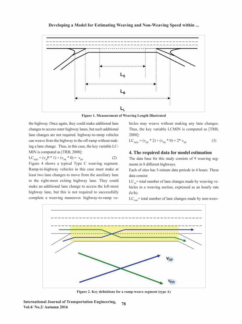
3. Physical and operational characteristics of principal arterial weaving3.1 The length of a weaving segmentThe lengths illustrated in Figure 1 are defined as follows [TRB, 2015]:
LS: Short Length, m; the distance between the end points of any barrier markings that prohibit or discourage lane-changing.LB: Base Length; m; the distance between points in the respective gore areas where the left edge of the ramp travel lanes and the right edge of the highway travel lanes meet.LL: Long Length, m; the distance between physical barri-ers marking the ends of the merge and diverge gore areas.The Project Team worked with three different defini-tions of length, as illustrated in Figure 1. It appears that LB would be the most logical measure of length [TCTTS, 2015].
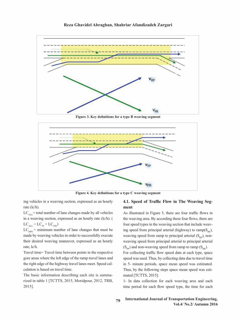
3.2 Lane ConfigurationLane configuration refers to the manner in which entry and exit legs connect. Figures 2, 3, and 4 show three examples which representing each of the three defined configura-tions in HCM2010, and illustrates the determination of these two key variables [TRB, 2008]. Figure 2 shows a typical 4-lane ramp-weaving segment, with a one-lane on-ramp followed by a one-lane off-ramp connected by a continuous auxiliary lane. On-ramp ve-hicles enter the segment on the auxiliary lane, and must execute one lane change to the right-most highway lane to complete their weaving maneuver. They could make ad-ditional lane changes to access outer lanes of the highway, but they do not have to do so to successfully weave. Simi-larly, off-ramp vehicles may enter the weaving segment on the right-most lane of the highway (although they could choose to enter on another lane and make multiple lane changes to access the auxiliary lane), and must exit on the auxiliary lane [TRB, 2008]. As each weaving vehicle must execute at least one lane change, the key variable LCMIN (= minimum number of lane changes that must be made by weaving vehicles in or-der to successfully execute their desired weaving maneu-ver, expressed as an hourly rate, lc/h) would be computed as follows (for more knowledge see 4.3.) [TRB, 2008]:LCMIN = (vRP * 1) + (vPR * 1) = vRP + vPR (1)For computational convenience, the algorithms use flow rates already converted to equivalent pc/h for this com-putation.Figure 3 shows a typical Type B weaving segment. Note that ramp-to-highway vehicles must make a single lane change to successfully weave onto the right-most lane of
Reza Ghavidel Abraghan, Shahriar Afandizadeh Zargari
78International Journal of Transportation Engineering, Vol.4/ No.2/ Autumn 2016
Figure 1. Measurement of Weaving Length Illustrated
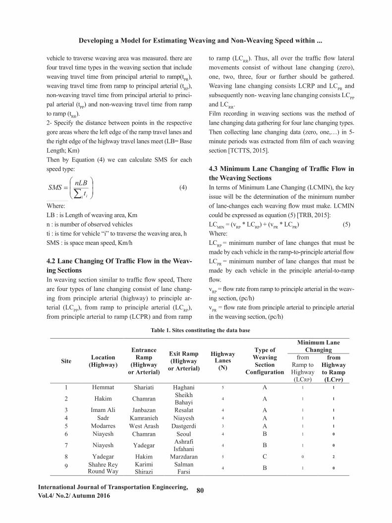
the highway. Once again, they could make additional lane changes to access outer highway lanes, but such additional lane changes are not required. highway-to-ramp vehicles can weave from the highway to the off-ramp without mak-ing a lane change. Thus, in this case, the key variable LC-MIN is computed as [TRB, 2008]: LCMIN = (vRP * 1) + (vPR * 0) = vRP (2)Figure 4 shows a typical Type C weaving segment. Ramp-to-highway vehicles in this case must make at least two lane changes to move from the auxiliary lane to the right-most exiting highway lane. They could make an additional lane change to access the left-most highway lane, but this is not required to successfully complete a weaving maneuver. highway-to-ramp ve-
hicles may weave without making any lane changes. Thus, the key variable LCMIN is computed as [TRB, 2008]:LCMIN = (vRP * 2) + (vPR * 0) = 2* vRP (3)
4. The required data for model estimationThe data base for this study consists of 9 weaving seg-ments in 8 different highways.Each of sites has 5-minute data periods in 4 hours. These data consist:LCW= total number of lane changes made by weaving ve-hicles in a weaving section, expressed as an hourly rate (lc/h). LCNW= total number of lane changes made by non-weav-
On the whole, capacity and level of service analysis in weaving segments has needed to estimate speed since 1985. In HCM 1985 and its updating at 1994, speed has been directly relevant to level of service. In 1997 updating and HCM 2000, speed has been estimated and subsequently has been converted to density and level of service has been calculated based on density. But in HCM 2010, methodology has changed; it means that in first step lane changing rate has been estimated and then speed has been estimated and subsequently speed has been converted to density and level of service has been calculated based on density [TRB, 2008]. These arguments show that speed estimation has ever been a foundation in weaving sections level of service analysis. In this essay, HCM 2010 concepts for developing speed estimation model, as a new approach, have been used [TCTTS, 2015].
3. Physical and operational characteristics of principal arterial weaving 3.1 The length of a weaving segment
The lengths illustrated in Figure 1 are defined as follows [TRB, 2015]: LS: Short Length, m; the distance between the end points of any barrier markings that prohibit
or discourage lane-changing. LB: Base Length; m; the distance between points in the respective gore areas where the left edge
of the ramp travel lanes and the right edge of the highway travel lanes meet.
LL: Long Length, m; the distance between physical barriers marking the ends of the merge and diverge gore areas.
The Project Team worked with three different definitions of length, as illustrated in Figure 1. It appears that LB would be the most logical measure of length [TCTTS, 2015].
Figure 1. Measurement of Weaving Length Illustrated
3.2 Lane Configuration
Lane configuration refers to the manner in which entry and exit legs connect. Figures 2, 3, and 4 show three examples which representing each of the three defined configurations in HCM2010, and illustrates the determination of these two key variables [TRB, 2008].
Figure 2 shows a typical 4-lane ramp-weaving segment, with a one-lane on-ramp followed by a one-lane off-ramp connected by a continuous auxiliary lane. On-ramp vehicles enter the segment on the auxiliary lane, and must execute one lane change to the right-most highway lane to complete their weaving maneuver. They could make additional lane changes to access outer lanes of the highway, but they do not have to do so to successfully weave. Similarly, off-ramp vehicles may enter the weaving segment on the right-most lane of the highway (although they could choose to enter on another lane and make multiple lane changes to access the auxiliary lane), and must exit on the auxiliary lane [TRB, 2008].
As each weaving vehicle must execute at least one lane change, the key variable LCMIN (= minimum number of lane changes that must be made by weaving vehicles in order to successfully execute their desired weaving maneuver, expressed as an hourly rate, lc/h) would be computed as follows (for more knowledge see 4.3.) [TRB, 2008]:
LCMIN = (vRP * 1) + (vPR * 1) = vRP + vPR (1) For computational convenience, the algorithms use flow rates already converted to equivalent
pc/h for this computation.
Figure 2. Key definitions for a ramp-weave segment (type A) Figure 2. Key definitions for a ramp-weave segment (type A)
Developing a Model for Estimating Weaving and Non-Weaving Speed within ...
79 International Journal of Transportation Engineering, Vol.4/ No.2/ Autumn 2016
Figure 3. Key definitions for a type B weaving segment
Figure 4. Key definitions for a type C weaving segment
Figure 3. Key definitions for a type B weaving segment
Figure 4. Key definitions for a type C weaving segment
Figure 3 shows a typical Type B weaving segment. Note that ramp-to-highway vehicles must make a single lane change to successfully weave onto the right-most lane of the highway. Once again, they could make additional lane changes to access outer highway lanes, but such additional lane changes are not required. highway-to-ramp vehicles can weave from the highway to the off-
ing vehicles in a weaving section, expressed as an hourly rate (lc/h).LCALL= total number of lane changes made by all vehicles in a weaving section, expressed as an hourly rate (lc/h). ( LCALL = LCW + LCNW)LCMIN = minimum number of lane changes that must be made by weaving vehicles in order to successfully execute their desired weaving maneuver, expressed as an hourly rate, lc/h.Travel time= Travel time between points in the respective gore areas where the left edge of the ramp travel lanes and the right edge of the highway travel lanes meet. Speed cal-culation is based on travel time.The basic information describing each site is summa-rized in table 1 [TCTTS, 2015, Moridpour, 2012, TRB, 2015].
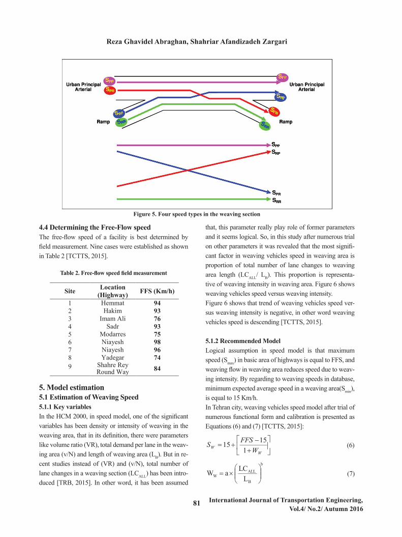
4.1. Speed of Traffic Flow in The Weaving Seg-mentAs illustrated in Figure 5, there are four traffic flows in the weaving area. By according these four flows, there are four speed types in the weaving section that include weav-ing speed from principal arterial (highway) to ramp(SPR), weaving speed from ramp to principal arterial (SRP), non-weaving speed from principal arterial to principal arterial (SPP) and non-weaving speed from ramp to ramp (SRR).For collecting traffic flow speed data at each type, space speed was used. Thus, by collecting data due to travel time in 5- minute periods, space mean speed was estimated. Thus, by the following steps space mean speed was esti-mated [TCTTS, 2015]:1- In data collection for each weaving area and each time period for each flow speed type, the time for each
Reza Ghavidel Abraghan, Shahriar Afandizadeh Zargari
80International Journal of Transportation Engineering, Vol.4/ No.2/ Autumn 2016
Table 1. Sites constituting the data base
vehicle to traverse weaving area was measured. there are four travel time types in the weaving section that include weaving travel time from principal arterial to ramp(tPR), weaving travel time from ramp to principal arterial (tRP), non-weaving travel time from principal arterial to princi-pal arterial (tPP) and non-weaving travel time from ramp to ramp (tRR).2- Specify the distance between points in the respective gore areas where the left edge of the ramp travel lanes and the right edge of the highway travel lanes meet (LB= Base Length; Km)Then by Equation (4) we can calculate SMS for each speed type:
Figure 5. Four speed types in the weaving section
Then by Equation (4) we can calculate SMS for each speed type:
4
i itnLBSMS
Where: LB : is Length of weaving area, Km n : is number of observed vehicles ti : is time for vehicle “i” to traverse the weaving area, h SMS : is space mean speed, Km/h
4.2 Lane Changing Of Traffic Flow in the Weaving Sections In weaving section similar to traffic flow speed, There are four types of lane changing consist
of lane changing from principle arterial (highway) to principle arterial (LCPP), from ramp to principle arterial (LCRP), from principle arterial to ramp (LCPR) and from ramp to ramp (LCRR). Thus, all over the traffic flow lateral movements consist of without lane changing (zero), one, two, three, four or further should be gathered. Weaving lane changing consists LCRP and LCPR and subsequently non- weaving lane changing consists LCPP and LCRR.
Film recording in weaving sections was the method of lane changing data gathering for four lane changing types. Then collecting lane changing data (zero, one,…) in 5- minute periods was extracted from film of each weaving section [TCTTS, 2015]. 4.3 Minimum Lane Changing of Traffic Flow in the Weaving Sections
(4)
Where:LB : is Length of weaving area, Kmn : is number of observed vehiclesti : is time for vehicle “i” to traverse the weaving area, hSMS : is space mean speed, Km/h
4.2 Lane Changing Of Traffic Flow in the Weav-ing SectionsIn weaving section similar to traffic flow speed, There are four types of lane changing consist of lane chang-ing from principle arterial (highway) to principle ar-terial (LCPP), from ramp to principle arterial (LCRP), from principle arterial to ramp (LCPR) and from ramp
to ramp (LCRR). Thus, all over the traffic flow lateral movements consist of without lane changing (zero), one, two, three, four or further should be gathered. Weaving lane changing consists LCRP and LCPR and subsequently non- weaving lane changing consists LCPP and LCRR.Film recording in weaving sections was the method of lane changing data gathering for four lane changing types. Then collecting lane changing data (zero, one,…) in 5- minute periods was extracted from film of each weaving section [TCTTS, 2015].
4.3 Minimum Lane Changing of Traffic Flow in the Weaving SectionsIn terms of Minimum Lane Changing (LCMIN), the key issue will be the determination of the minimum number of lane-changes each weaving flow must make. LCMIN could be expressed as equation (5) [TRB, 2015]: LCMIN = (vRP * LCRP) + (vPR * LCPR) (5)Where: LCRP = minimum number of lane changes that must be made by each vehicle in the ramp-to-principle arterial flowLCPR = minimum number of lane changes that must be made by each vehicle in the principle arterial-to-ramp flow.vRP = flow rate from ramp to principle arterial in the weav-ing section, (pc/h)vPR = flow rate from principle arterial to principle arterial in the weaving section, (pc/h)
Minimum Lane Changing Type of
Weaving Section
Configuration
Highway Lanes
(N)
Exit Ramp (Highway
or Arterial)
Entrance Ramp
(Highway or Arterial)
Location (Highway) Site from
Highway to Ramp (LCPP)
from Ramp to Highway (LCRP)
1 1 A 5 Haghani Shariati Hemmat 1
1 1 A 4 Sheikh Bahayi Chamran Hakim 2
1 1 A 4 Resalat Janbazan Imam Ali 3 1 1 A 4 Niayesh Kamranieh Sadr 4 1 1 A 3 Dastgerdi West Arash Modarres 5 0 1 B 4 Seoul Chamran Niayesh 6
0 1 B 4 Ashrafi Isfahani Yadegar Niayesh 7
2 0 C 5 Marzdaran Hakim Yadegar 8
0 1 B 4 Salman Farsi
Karimi Shirazi
Shahre Rey Round Way
9
4.1. Speed of Traffic Flow in The Weaving Segment
As illustrated in Figure 5, there are four traffic flows in the weaving area. By according these four flows, there are four speed types in the weaving section that include weaving speed from principal arterial (highway) to ramp(SPR), weaving speed from ramp to principal arterial (SRP), non-weaving speed from principal arterial to principal arterial (SPP) and non-weaving speed from ramp to ramp (SRR).
For collecting traffic flow speed data at each type, space speed was used. Thus, by collecting data due to travel time in 5- minute periods, space mean speed was estimated. Thus, by the following steps space mean speed was estimated [TCTTS, 2015]:
1- In data collection for each weaving area and each time period for each flow speed type, the time for each vehicle to traverse weaving area was measured. there are four travel time types in the weaving section that include weaving travel time from principal arterial to ramp(tPR), weaving travel time from ramp to principal arterial (tRP), non-weaving travel time from principal arterial to principal arterial (tPP) and non-weaving travel time from ramp to ramp (tRR).
2- Specify the distance between points in the respective gore areas where the left edge of the ramp
travel lanes and the right edge of the highway travel lanes meet (LB= Base Length; Km)
Developing a Model for Estimating Weaving and Non-Weaving Speed within ...
81 International Journal of Transportation Engineering, Vol.4/ No.2/ Autumn 2016
Figure 5. Four speed types in the weaving section
Figure 5. Four speed types in the weaving section
Then by Equation (4) we can calculate SMS for each speed type:
4
i itnLBSMS
Where: LB : is Length of weaving area, Km n : is number of observed vehicles ti : is time for vehicle “i” to traverse the weaving area, h SMS : is space mean speed, Km/h
4.2 Lane Changing Of Traffic Flow in the Weaving Sections In weaving section similar to traffic flow speed, There are four types of lane changing consist
of lane changing from principle arterial (highway) to principle arterial (LCPP), from ramp to principle arterial (LCRP), from principle arterial to ramp (LCPR) and from ramp to ramp (LCRR). Thus, all over the traffic flow lateral movements consist of without lane changing (zero), one, two, three, four or further should be gathered. Weaving lane changing consists LCRP and LCPR and subsequently non- weaving lane changing consists LCPP and LCRR.
Film recording in weaving sections was the method of lane changing data gathering for four lane changing types. Then collecting lane changing data (zero, one,…) in 5- minute periods was extracted from film of each weaving section [TCTTS, 2015]. 4.3 Minimum Lane Changing of Traffic Flow in the Weaving Sections
4.4 Determining the Free-Flow speedThe free-flow speed of a facility is best determined by field measurement. Nine cases were established as shown in Table 2 [TCTTS, 2015].
Table 2. Free-flow speed field measurement
In terms of Minimum Lane Changing (LCMIN), the key issue will be the determination of the minimum number of lane-changes each weaving flow must make. LCMIN could be expressed as equation (5) [TRB, 2015]:
LCMIN = (vRP * LCRP) + (vPR * LCPR) (5) Where: LCRP = minimum number of lane changes that must be made by each vehicle in the ramp-to-principle arterial flow LCPR = minimum number of lane changes that must be made by each vehicle in the principle arterial-to-ramp flow. vRP = flow rate from ramp to principle arterial in the weaving section, (pc/h)
vPR = flow rate from principle arterial to principle arterial in the weaving section, (pc/h)
4.4 Determining the Free-Flow speed The free-flow speed of a facility is best determined by field measurement. Nine cases were established as shown in Table 2 [TCTTS, 2015].
Table 2. Free-flow speed field measurement
FFS (Km/h) Location (Highway) Site
94 Hemmat 1 93 Hakim 2 76 Imam Ali 3 93 Sadr 4 75 Modarres 5 98 Niayesh 6 96 Niayesh 7 74 Yadegar 8 84 Shahre Rey
Round Way 9
5. Model estimation 5.1 Estimation of Weaving Speed 5.1.1 Key variables
In the HCM 2000, in speed model, one of the significant variables has been density or intensity of weaving in the weaving area, that in its definition, there were parameters like volume ratio (VR),
5. Model estimation5.1 Estimation of Weaving Speed5.1.1 Key variablesIn the HCM 2000, in speed model, one of the significant variables has been density or intensity of weaving in the weaving area, that in its definition, there were parameters like volume ratio (VR), total demand per lane in the weav-ing area (v/N) and length of weaving area (LB). But in re-cent studies instead of (VR) and (v/N), total number of lane changes in a weaving section (LCALL) has been intro-duced [TRB, 2015]. In other word, it has been assumed
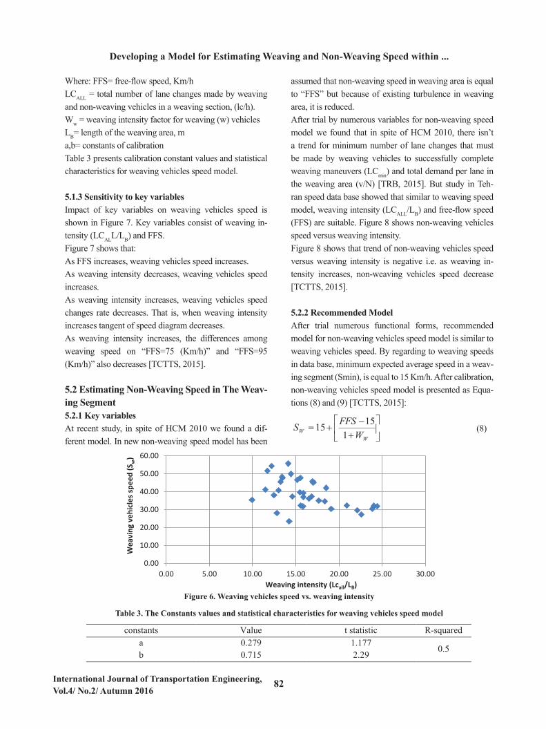
that, this parameter really play role of former parameters and it seems logical. So, in this study after numerous trial on other parameters it was revealed that the most signifi-cant factor in weaving vehicles speed in weaving area is proportion of total number of lane changes to weaving area length (LCALL/ LB). This proportion is representa-tive of weaving intensity in weaving area. Figure 6 shows weaving vehicles speed versus weaving intensity.Figure 6 shows that trend of weaving vehicles speed ver-sus weaving intensity is negative, in other word weaving vehicles speed is descending [TCTTS, 2015].
5.1.2 Recommended ModelLogical assumption in speed model is that maximum speed (Smax) in basic area of highways is equal to FFS, and weaving flow in weaving area reduces speed due to weav-ing intensity. By regarding to weaving speeds in database, minimum expected average speed in a weaving area(Smin), is equal to 15 Km/h.In Tehran city, weaving vehicles speed model after trial of numerous functional form and calibration is presented as Equations (6) and (7) [TCTTS, 2015]:
total demand per lane in the weaving area (v/N) and length of weaving area (LB). But in recent studies instead of (VR) and (v/N), total number of lane changes in a weaving section (LCALL) has been introduced [TRB, 2015]. In other word, it has been assumed that, this parameter really play role of former parameters and it seems logical. So, in this study after numerous trial on other parameters it was revealed that the most significant factor in weaving vehicles speed in weaving area is proportion of total number of lane changes to weaving area length (LCALL/ LB). This proportion is representative of weaving intensity in weaving area. Figure 6 shows weaving vehicles speed versus weaving intensity.
Figure 6. Weaving vehicles speed vs. weaving intensity
Figure 6 shows that trend of weaving vehicles speed versus weaving intensity is negative, in
other word weaving vehicles speed is descending [TCTTS, 2015].
5.1.2 Recommended Model Logical assumption in speed model is that maximum speed (Smax) in basic area of highways is
equal to FFS, and weaving flow in weaving area reduces speed due to weaving intensity. By regarding to weaving speeds in database, minimum expected average speed in a weaving area(Smin), is equal to 15 Km/h.
In Tehran city, weaving vehicles speed model after trial of numerous functional form and calibration is presented as Equations (6) and (7) [TCTTS, 2015]:
6
W
W WFFSS1
1515
7 b
B
ALLW L
LCaW
Where: FFS= free-flow speed, Km/h LCALL = total number of lane changes made by weaving and non-weaving vehicles in a weaving
section, (lc/h).
0.00
10.00
20.00
30.00
40.00
50.00
60.00
0.00 5.00 10.00 15.00 20.00 25.00 30.00
Wea
ving
veh
icle
s spe
ed (S
w)
Weaving intensity (Lcall/LB)
(6)
total demand per lane in the weaving area (v/N) and length of weaving area (LB). But in recent studies instead of (VR) and (v/N), total number of lane changes in a weaving section (LCALL) has been introduced [TRB, 2015]. In other word, it has been assumed that, this parameter really play role of former parameters and it seems logical. So, in this study after numerous trial on other parameters it was revealed that the most significant factor in weaving vehicles speed in weaving area is proportion of total number of lane changes to weaving area length (LCALL/ LB). This proportion is representative of weaving intensity in weaving area. Figure 6 shows weaving vehicles speed versus weaving intensity.
Figure 6. Weaving vehicles speed vs. weaving intensity
Figure 6 shows that trend of weaving vehicles speed versus weaving intensity is negative, in
other word weaving vehicles speed is descending [TCTTS, 2015].
5.1.2 Recommended Model Logical assumption in speed model is that maximum speed (Smax) in basic area of highways is
equal to FFS, and weaving flow in weaving area reduces speed due to weaving intensity. By regarding to weaving speeds in database, minimum expected average speed in a weaving area(Smin), is equal to 15 Km/h.
In Tehran city, weaving vehicles speed model after trial of numerous functional form and calibration is presented as Equations (6) and (7) [TCTTS, 2015]:
6
W
W WFFSS1
1515
7 b
B
ALLW L
LCaW
Where: FFS= free-flow speed, Km/h LCALL = total number of lane changes made by weaving and non-weaving vehicles in a weaving
section, (lc/h).
0.00
10.00
20.00
30.00
40.00
50.00
60.00
0.00 5.00 10.00 15.00 20.00 25.00 30.00
Wea
ving
veh
icle
s spe
ed (S
w)
Weaving intensity (Lcall/LB)
(7)
Reza Ghavidel Abraghan, Shahriar Afandizadeh Zargari
82International Journal of Transportation Engineering, Vol.4/ No.2/ Autumn 2016
Where: FFS= free-flow speed, Km/hLCALL = total number of lane changes made by weaving and non-weaving vehicles in a weaving section, (lc/h).Ww = weaving intensity factor for weaving (w) vehiclesLB= length of the weaving area, ma,b= constants of calibrationTable 3 presents calibration constant values and statistical characteristics for weaving vehicles speed model.
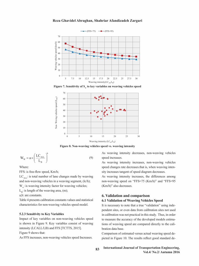
5.1.3 Sensitivity to key variablesImpact of key variables on weaving vehicles speed is shown in Figure 7. Key variables consist of weaving in-tensity (LCALL/LB) and FFS.Figure 7 shows that:As FFS increases, weaving vehicles speed increases.As weaving intensity decreases, weaving vehicles speed increases.As weaving intensity increases, weaving vehicles speed changes rate decreases. That is, when weaving intensity increases tangent of speed diagram decreases.As weaving intensity increases, the differences among weaving speed on “FFS=75 (Km/h)” and “FFS=95 (Km/h)” also decreases [TCTTS, 2015].
5.2 Estimating Non-Weaving Speed in The Weav-ing Segment5.2.1 Key variables At recent study, in spite of HCM 2010 we found a dif-ferent model. In new non-weaving speed model has been
assumed that non-weaving speed in weaving area is equal to “FFS” but because of existing turbulence in weaving area, it is reduced.After trial by numerous variables for non-weaving speed model we found that in spite of HCM 2010, there isn’t a trend for minimum number of lane changes that must be made by weaving vehicles to successfully complete weaving maneuvers (LCmin) and total demand per lane in the weaving area (v/N) [TRB, 2015]. But study in Teh-ran speed data base showed that similar to weaving speed model, weaving intensity (LCALL/LB) and free-flow speed (FFS) are suitable. Figure 8 shows non-weaving vehicles speed versus weaving intensity.Figure 8 shows that trend of non-weaving vehicles speed versus weaving intensity is negative i.e. as weaving in-tensity increases, non-weaving vehicles speed decrease [TCTTS, 2015].
5.2.2 Recommended ModelAfter trial numerous functional forms, recommended model for non-weaving vehicles speed model is similar to weaving vehicles speed. By regarding to weaving speeds in data base, minimum expected average speed in a weav-ing segment (Smin), is equal to 15 Km/h. After calibration, non-weaving vehicles speed model is presented as Equa-tions (8) and (9) [TCTTS, 2015]:
Figure 8. Non-weaving vehicles speed vs. weaving intensity
Figure 8 shows that trend of non-weaving vehicles speed versus weaving intensity is negative
i.e. as weaving intensity increases, non-weaving vehicles speed decrease [TCTTS, 2015].
5.2.2 Recommended Model After trial numerous functional forms, recommended model for non-weaving vehicles speed
model is similar to weaving vehicles speed. By regarding to weaving speeds in data base, minimum expected average speed in a weaving segment (Smin), is equal to 15 Km/h. After calibration, non-weaving vehicles speed model is presented as Equations (8) and (9) [TCTTS, 2015]:
8
W
W WFFSS1
1515
9 b
B
ALLW L
LCaW
Where: FFS: is free-flow speed, Km/h; LCALL: is total number of lane changes made by weaving and non-weaving vehicles in a
weaving segment, (lc/h); Ww: is weaving intensity factor for weaving vehicles; LB: is length of the weaving area, (m); a,b: are constants. Table 4 presents calibration constants values and statistical characteristics for non-weaving
vehicles speed model.
Table 4. The Constants values and statistical characteristics for non-weaving vehicles speed model
0
10
20
30
40
50
60
70
0 5 10 15 20 25 30
Non
-Wev
ing
vehi
cles
spee
d (S
NW
)
Weaving intensity (LCall/LB)
(8)
Figure 6. Weaving vehicles speed vs. weaving intensity
Table 3. The Constants values and statistical characteristics for weaving vehicles speed model
total demand per lane in the weaving area (v/N) and length of weaving area (LB). But in recent studies instead of (VR) and (v/N), total number of lane changes in a weaving section (LCALL) has been introduced [TRB, 2015]. In other word, it has been assumed that, this parameter really play role of former parameters and it seems logical. So, in this study after numerous trial on other parameters it was revealed that the most significant factor in weaving vehicles speed in weaving area is proportion of total number of lane changes to weaving area length (LCALL/ LB). This proportion is representative of weaving intensity in weaving area. Figure 6 shows weaving vehicles speed versus weaving intensity.
Figure 6. Weaving vehicles speed vs. weaving intensity
Figure 6 shows that trend of weaving vehicles speed versus weaving intensity is negative, in
other word weaving vehicles speed is descending [TCTTS, 2015].
5.1.2 Recommended Model Logical assumption in speed model is that maximum speed (Smax) in basic area of highways is
equal to FFS, and weaving flow in weaving area reduces speed due to weaving intensity. By regarding to weaving speeds in database, minimum expected average speed in a weaving area(Smin), is equal to 15 Km/h.
In Tehran city, weaving vehicles speed model after trial of numerous functional form and calibration is presented as Equations (6) and (7) [TCTTS, 2015]:
6
W
W WFFSS1
1515
7 b
B
ALLW L
LCaW
Where: FFS= free-flow speed, Km/h LCALL = total number of lane changes made by weaving and non-weaving vehicles in a weaving
section, (lc/h).
0.00
10.00
20.00
30.00
40.00
50.00
60.00
0.00 5.00 10.00 15.00 20.00 25.00 30.00
Wea
ving
veh
icle
s spe
ed (S
w)
Weaving intensity (Lcall/LB)
Ww = weaving intensity factor for weaving (w) vehicles LB= length of the weaving area, m a,b= constants of calibration Table 3 presents calibration constant values and statistical characteristics for weaving vehicles
speed model.
Table 3. The Constants values and statistical characteristics for weaving vehicles speed model constants Value t statistic R-squared
a 0.279 1.177 0.5
b 0.715 2.29
Developing a Model for Estimating Weaving and Non-Weaving Speed within ...
83 International Journal of Transportation Engineering, Vol.4/ No.2/ Autumn 2016
Figure 8. Non-weaving vehicles speed vs. weaving intensity
Figure 8 shows that trend of non-weaving vehicles speed versus weaving intensity is negative
i.e. as weaving intensity increases, non-weaving vehicles speed decrease [TCTTS, 2015].
5.2.2 Recommended Model After trial numerous functional forms, recommended model for non-weaving vehicles speed
model is similar to weaving vehicles speed. By regarding to weaving speeds in data base, minimum expected average speed in a weaving segment (Smin), is equal to 15 Km/h. After calibration, non-weaving vehicles speed model is presented as Equations (8) and (9) [TCTTS, 2015]:
8
W
W WFFSS1
1515
9 b
B
ALLW L
LCaW
Where: FFS: is free-flow speed, Km/h; LCALL: is total number of lane changes made by weaving and non-weaving vehicles in a
weaving segment, (lc/h); Ww: is weaving intensity factor for weaving vehicles; LB: is length of the weaving area, (m); a,b: are constants. Table 4 presents calibration constants values and statistical characteristics for non-weaving
vehicles speed model.
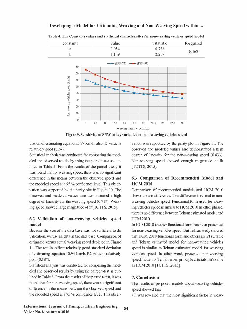
Table 4. The Constants values and statistical characteristics for non-weaving vehicles speed model
0
10
20
30
40
50
60
70
0 5 10 15 20 25 30
Non
-Wev
ing
vehi
cles
spee
d (S
NW
)
Weaving intensity (LCall/LB)
(9)
Where:FFS: is free-flow speed, Km/h;LCALL: is total number of lane changes made by weaving and non-weaving vehicles in a weaving segment, (lc/h);Ww: is weaving intensity factor for weaving vehicles;LB: is length of the weaving area, (m);a,b: are constants.Table 4 presents calibration constants values and statistical characteristics for non-weaving vehicles speed model.
5.2.3 Sensitivity to Key VariablesImpact of key variables on non-weaving vehicles speed is shown in Figure 9. Key variables consist of weaving intensity (LCALL/LB) and FFS [TCTTS, 2015].Figure 9 shows that:As FFS increases, non-weaving vehicles speed Increases.
As weaving intensity decreases, non-weaving vehicles speed increases.As weaving intensity increases, non-weaving vehicles speed changes rate decreases.that is, when weaving inten-sity increases tangent of speed diagram decreases.As weaving intensity increases, the differences among non-weaving speed on “FFS=75 (Km/h)” and “FFS=95 (Km/h)” also decreases. 6. Validation and comparison6.1 Validation of Weaving Vehicles SpeedIt is necessary to note that a true “validation” using inde-pendent sites, or even data from calibration sites not used in calibration was not practical in this study. Thus, in order to measure the accuracy of the developed models estima-tions of weaving speed are compared directly to the cali-bration data base.Comparison of estimated versus actual weaving speed de-picted in Figure 10. The results reflect good standard de-
Figure 7. Sensitivity of Sw to key variables on weaving vehicles speed
Figure 8. Non-weaving vehicles speed vs. weaving intensity
5.1.3 Sensitivity to key variables Impact of key variables on weaving vehicles speed is shown in Figure 7. Key variables consist
of weaving intensity (LCALL/LB) and FFS. Figure 7 shows that: As FFS increases, weaving vehicles speed increases. As weaving intensity decreases, weaving vehicles speed increases. As weaving intensity increases, weaving vehicles speed changes rate decreases. That is, when
weaving intensity increases tangent of speed diagram decreases. As weaving intensity increases, the differences among weaving speed on “FFS=75 (Km/h)”
and “FFS=95 (Km/h)” also decreases [TCTTS, 2015].
variables on weaving vehicles speed key to wof SSensitivity . 7 Figure
5.2 Estimating Non-Weaving Speed in The Weaving Segment 5.2.1 Key variables
At recent study, in spite of HCM 2010 we found a different model. In new non-weaving speed model has been assumed that non-weaving speed in weaving area is equal to “FFS” but because of existing turbulence in weaving area, it is reduced.
After trial by numerous variables for non-weaving speed model we found that in spite of HCM 2010, there isn’t a trend for minimum number of lane changes that must be made by weaving vehicles to successfully complete weaving maneuvers (LCmin) and total demand per lane in the weaving area (v/N) [TRB, 2015]. But study in Tehran speed data base showed that similar to weaving speed model, weaving intensity (LCALL/LB) and free-flow speed (FFS) are suitable. Figure 8 shows non-weaving vehicles speed versus weaving intensity.
0
10
20
30
40
50
60
70
5 7.5 10 12.5 15 17.5 20 22.5 25 27.5 30
Wea
ving
veh
icle
s spe
ed (k
m/h
)
Weaving intensity(LCAll/LB)
(FFS=75) (FFS=95)
Figure 8. Non-weaving vehicles speed vs. weaving intensity
Figure 8 shows that trend of non-weaving vehicles speed versus weaving intensity is negative
i.e. as weaving intensity increases, non-weaving vehicles speed decrease [TCTTS, 2015].
5.2.2 Recommended Model After trial numerous functional forms, recommended model for non-weaving vehicles speed
model is similar to weaving vehicles speed. By regarding to weaving speeds in data base, minimum expected average speed in a weaving segment (Smin), is equal to 15 Km/h. After calibration, non-weaving vehicles speed model is presented as Equations (8) and (9) [TCTTS, 2015]:
8
W
W WFFSS1
1515
9 b
B
ALLW L
LCaW
Where: FFS: is free-flow speed, Km/h; LCALL: is total number of lane changes made by weaving and non-weaving vehicles in a
weaving segment, (lc/h); Ww: is weaving intensity factor for weaving vehicles; LB: is length of the weaving area, (m); a,b: are constants. Table 4 presents calibration constants values and statistical characteristics for non-weaving
vehicles speed model.
Table 4. The Constants values and statistical characteristics for non-weaving vehicles speed model
0
10
20
30
40
50
60
70
0 5 10 15 20 25 30
Non
-Wev
ing
vehi
cles
spee
d (S
NW
)
Weaving intensity (LCall/LB)
Reza Ghavidel Abraghan, Shahriar Afandizadeh Zargari
84International Journal of Transportation Engineering, Vol.4/ No.2/ Autumn 2016
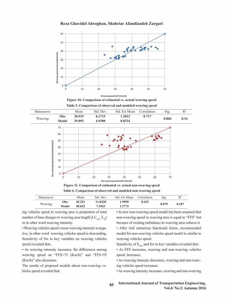
viation of estimating equation 5.77 Km/h. also, R2 value is relatively good (0.34).Statistical analysis was conducted for comparing the mod-eled and observed results by using the paired t-test as out-lined in Table 5. From the results of the paired t-test, it was found that for weaving speed, there was no significant difference in the means between the observed speed and the modeled speed at a 95 % confidence level. This obser-vation was supported by the parity plot in Figure 10. The observed and modeled values also demonstrated a high degree of linearity for the weaving speed (0.717). Weav-ing speed showed large magnitude of fit[TCTTS, 2015].
6.2 Validation of non-weaving vehicles speed modelBecause the size of the data base was not sufficient to do validation, we use all data in the data base. Comparison of estimated versus actual weaving speed depicted in Figure 11. The results reflect relatively good standard deviation of estimating equation 10.94 Km/h. R2 value is relatively poor (0.187).Statistical analysis was conducted for comparing the mod-eled and observed results by using the paired t-test as out-lined in Table 6. From the results of the paired t-test, it was found that for non-weaving speed, there was no significant difference in the means between the observed speed and the modeled speed at a 95 % confidence level. This obser-
vation was supported by the parity plot in Figure 11. The observed and modeled values also demonstrated a high degree of linearity for the non-weaving speed (0.433). Non-weaving speed showed enough magnitude of fit [TCTTS, 2015].
6.3 Comparison of Recommended Model and HCM 2010 Comparison of recommended models and HCM 2010 shows a main difference. This difference is related to non-weaving vehicles speed. Functional form used for weav-ing vehicles speed is similar to HCM 2010 In other phrase, there is no difference between Tehran estimated model and HCM 2010.In HCM 2010 another functional form has been presented for non-weaving vehicles speed. But Tehran study showed that HCM 2010 functional form and others aren’t suitable and Tehran estimated model for non-weaving vehicles speed is similar to Tehran estimated model for weaving vehicles speed. In other word, presented non-weaving speed model for Tehran urban principle arterials isn’t same as HCM 2010 [TCTTS, 2015].
7. ConclusionThe results of proposed models about weaving vehicles speed showed that:• It was revealed that the most significant factor in weav-
Table 4. The Constants values and statistical characteristics for non-weaving vehicles speed model
constants Value t statistic R-squared a 0.054 0.738 0.463 b 1.109 2.268
5.2.3 Sensitivity to Key Variables Impact of key variables on non-weaving vehicles speed is shown in Figure 9. Key variables
consist of weaving intensity (LCALL/LB) and FFS [TCTTS, 2015].
Figure 9. Sensitivity of SNW to key variables on non-weaving vehicles speed
Figure 9 shows that: As FFS increases, non-weaving vehicles speed Increases. As weaving intensity decreases, non-weaving vehicles speed increases. As weaving intensity increases, non-weaving vehicles speed changes rate decreases.that is,
when weaving intensity increases tangent of speed diagram decreases. As weaving intensity increases, the differences among non-weaving speed on “FFS=75
(Km/h)” and “FFS=95 (Km/h)” also decreases.
0
10
20
30
40
50
60
70
80
5 7.5 10 12.5 15 17.5 20 22.5 25 27.5 30
Non
-wea
ving
veh
icle
s spe
ed (k
m/h
)
Weaving intensity(LCAll/LB)
(FFS=75) (FFS=95)
Figure 9. Sensitivity of SNW to key variables on non-weaving vehicles speed
Developing a Model for Estimating Weaving and Non-Weaving Speed within ...
85 International Journal of Transportation Engineering, Vol.4/ No.2/ Autumn 2016
ing vehicles speed in weaving area is proportion of total number of lane changes to weaving area length (LCALL/LB) or in other word weaving intensity.• Weaving vehicles speed versus weaving intensity is nega-tive, in other word weaving vehicles speed is descending.Sensitivity of Sw to key variables on weaving vehicles speed revealed that:.• As weaving intensity increases, the differences among weaving speed on “FFS=75 (Km/h)” and “FFS=95 (Km/h)” also decreases.The results of proposed models about non-weaving ve-hicles speed revealed that:
• In new non-weaving speed model has been assumed that non-weaving speed in weaving area is equal to “FFS” but because of existing turbulence in weaving area reduces it.• After trial numerous functional forms, recommended model for non-weaving vehicles speed model is similar to weaving vehicles speed.Sensitivity of SNW and Sw to key variables revealed that:• As FFS increases, weaving and non-weaving vehicles speed. Increases.• As weaving intensity decreases, weaving and non-weav-ing vehicles speed increases.• As weaving intensity increases, weaving and non-weaving
6. Validation and comparison 6.1 Validation of Weaving Vehicles Speed
It is necessary to note that a true “validation” using independent sites, or even data from calibration sites not used in calibration was not practical in this study. Thus, in order to measure the accuracy of the developed models estimations of weaving speed are compared directly to the calibration data base.
Comparison of estimated versus actual weaving speed depicted in Figure 10. The results reflect good standard deviation of estimating equation 5.77 Km/h. also, R2 value is relatively good (0.34).
vs. actual weaving speed estimated. Comparison of 10 Figure
Statistical analysis was conducted for comparing the modeled and observed results by using the
paired t-test as outlined in Table 5. From the results of the paired t-test, it was found that for weaving speed, there was no significant difference in the means between the observed speed and the modeled speed at a 95 % confidence level. This observation was supported by the parity plot in Figure 10. The observed and modeled values also demonstrated a high degree of linearity for the weaving speed (0.717). Weaving speed showed large magnitude of fit[TCTTS, 2015].
weaving speed modeledomparison of observed and C .5Table
0
10
20
30
40
50
60
0 10 20 30 40 50 60
Wea
ving
spee
d (e
stim
ated
) (Km
/h)
Weaving speed (ACT) (Km/h)
Figure 10. Comparison of estimated vs. actual weaving speedTable 5. Comparison of observed and modeled weaving speed
Manoeuvre Mean Std. Dev. Std. Err Mean Correlation Sig. R2
Weaving Obs 38.919 8.1715 1.3812 0.717 0.860 0.34 Model 39.092 4.9308 0.8334
6.2 Validation of non-weaving vehicles speed model
Because the size of the data base was not sufficient to do validation, we use all data in the data base. Comparison of estimated versus actual weaving speed depicted in Figure 11. The results reflect relatively good standard deviation of estimating equation 10.94 Km/h. R2 value is relatively poor (0.187).
weaving speed-vs. actual non estimated. Comparison of 11 Figure
Statistical analysis was conducted for comparing the modeled and observed results by using the paired t-test as outlined in Table 6. From the results of the paired t-test, it was found that for non-weaving speed, there was no significant difference in the means between the observed speed and the modeled speed at a 95 % confidence level. This observation was supported by the parity plot in Figure 11. The observed and modeled values also demonstrated a high degree of linearity for the non-weaving speed (0.433). Non-weaving speed showed enough magnitude of fit [TCTTS, 2015].
weaving speed-nonomparison of observed and modeled C. 6Table
0
10
20
30
40
50
60
70
0 10 20 30 40 50 60 70Non
-wea
ving
spee
d (e
stim
ated
) (Km
/h)
Non-weaving speed (ACT) (Km/h)
Figure 11. Comparison of estimated vs. actual non-weaving speedTable 6. Comparison of observed and modeled non-weaving speed
Manoeuvre Mean Std. Dev. Std. Err Mean Correlation Sig. R2
Weaving Obs 45.251 11.8320 1.9999 0.433 0.075 0.187 Model 48.652 7.5563 1.2772
6.3 Comparison of Recommended Model and HCM 2010
Comparison of recommended models and HCM 2010 shows a main difference. This difference is related to non-weaving vehicles speed. Functional form used for weaving vehicles speed is similar to HCM 2010 In other phrase, there is no difference between Tehran estimated model and HCM 2010.
In HCM 2010 another functional form has been presented for non-weaving vehicles speed. But Tehran study showed that HCM 2010 functional form and others aren’t suitable and Tehran estimated model for non-weaving vehicles speed is similar to Tehran estimated model for weaving vehicles speed. In other word, presented non-weaving speed model for Tehran urban principle arterials isn’t same as HCM 2010 [TCTTS, 2015].
7. Conclusion The results of proposed models about weaving vehicles speed showed that: It was revealed that the most significant factor in weaving vehicles speed in weaving area is proportion of total number of lane changes to weaving area length (LCALL/LB) or in other word weaving intensity. Weaving vehicles speed versus weaving intensity is negative, in other word weaving vehicles speed is descending. Sensitivity of Sw to key variables on weaving vehicles speed revealed that:. As weaving intensity increases, the differences among weaving speed on “FFS=75 (Km/h)” and “FFS=95 (Km/h)” also decreases.
The results of proposed models about non-weaving vehicles speed revealed that: In new non-weaving speed model has been assumed that non-weaving speed in weaving area is equal to “FFS” but because of existing turbulence in weaving area reduces it. After trial numerous functional forms, recommended model for non-weaving vehicles speed model is similar to weaving vehicles speed. Sensitivity of SNW and Sw to key variables revealed that: As FFS increases, weaving and non-weaving vehicles speed. Increases. As weaving intensity decreases, weaving and non-weaving vehicles speed increases. As weaving intensity increases, weaving and non-weaving vehicles speed changes rate decreases. That is, when weaving intensity increases tangent of speed diagram decreases. As weaving intensity increases, the differences among non-weaving speed on “FFS=75 (Km/h)” and “FFS=95 (Km/h)” also decreases. As weaving intensity increases, the differences among weaving speed on “FFS=75 (Km/h)” and “FFS=95 (Km/h)” also decreases.
Comparison of Tehran recommended models and HCM 2010 shows a main difference. This difference is related to non-weaving vehicles speed, but functional form used for weaving vehicles speed is similar to HCM 2010 [TCTTS, 2015].
Reza Ghavidel Abraghan, Shahriar Afandizadeh Zargari
86International Journal of Transportation Engineering, Vol.4/ No.2/ Autumn 2016
vehicles speed changes rate decreases. That is, when weav-ing intensity increases tangent of speed diagram decreases.• As weaving intensity increases, the differences among non-weaving speed on “FFS=75 (Km/h)” and “FFS=95 (Km/h)” also decreases.• As weaving intensity increases, the differences among weaving speed on “FFS=75 (Km/h)” and “FFS=95 (Km/h)” also decreases.Comparison of Tehran recommended models and HCM 2010 shows a main difference. This difference is related to non-weaving vehicles speed, but functional form used for weaving vehicles speed is similar to HCM 2010 [TCTTS, 2015]. 8. References- Cassidy, M., Chan, P., Robinson, B. and May, A. D. (1990) “A proposed technique for the design and analy-sis of major freeway weaving sections”, Research Report UCB-ITS-RR-90-16, Institute of Transportation Studies, University of California – Berkeley, Berkeley CA.
- Cassidy, M., and May , A.D. (1991) ” Proposed ana-lytic technique for estimating capacity and level of ser-vice of major freeway weaving sections”, Transportation Research Record 1320, Transportation Research Board, Washington DC.
- Fazio, J. (1985) “Development and testing of a weaving operational design and analysis procedures”, M.S. Thesis, University of Illinois at Chicago Circle, Chicago IL.
Leisch, J. (1983) “Completion of Procedures for Analysis of and Design of Traffic Weaving Areas”, Final Report, Vols 1 and 2, U.S. Department of Transportation, Federal Highway Administration, Washington DC.
- Moridpour, S., Sarvi, M., Rose, G., Mazloumi Shomali, E. (2012) “Lane-changing decision model for heavy ve-hicle drivers”, Journal of Intelligent Transportation Sys-tems: technology, planning, and operations, vol 16, issue 1, Taylor & Francis, USA, pp. 24-35.
- Pignataro, L.J. , McShane, W.R. , and Roess, R.P. (1975) “Weaving Areas- Design and Analysis”, National Cooperative Highway Research Report 159, Transporta-
tion Research Board, Washington DC.
- Roess, R.P. , Prassas, E.S. (2014) “the highway capacity manual: A conceptual and research history springer tracts on transportation and traffic”, Volume 5.
- Reilly, W., Kell, J., and Johnson, P. (1984) “Weav-ing analysis procedures for the new highway capacity manual”, Technical Report, Contract No. DOT-FH-61-83-C-00029, U.S. Department of Transportation, Federal Highway Administration, Washington DC.
Sarvi, M., Ejtemai, O., Zavabeti, S. (2011) “ Modelling freeway weaving maneuver”, Proceedings of ATRF 2011 - 34th Australasian Transport Research Forum, 28 Septem-ber 2011 to 30 September 2011, Australasian Transport Research Forum, Adelaide SA, pp. 1-16
- Sarvi, M. (2014) “Freeway weaving phenomena ob-served during congested traffic”, Transportmetrica A: Transport Science, vol 9, issue 4, Taylor & Francis, Abing-don OX UK, pp. 299-315.
- Tehran Comprehensive Transportation and Traffic Stud-ies Company (2014) “codification criteria for access man-agement and weaving section length specification in urban roads”, Report 540. - Transportation Research Board (2008) “Analysis of free-way weaving sections”, Final Report.
- Transportation Research Board (1980), “Interim Materi-als on Highway Capacity”, Circular 212, Washington DC.
- Transportation Research Board Publication (2014) “The fourth Edition of the Highway Capacity Manual” (HCM2010).
- Windover, J. and May, A. D. (1995) “Revisions to level d methodology of analyzing freeway ramp-weaving sec-tions”, Transportation Research Record 1457, Transporta-tion Research Board, Washington DC.
Developing a Model for Estimating Weaving and Non-Weaving Speed within ...