
Detroit back from the brink? Auto industry crisis and ...
40
35 Federal Reserve Bank of Chicago Detroit back from the brink? Auto industry crisis and restructuring, 2008–11 Thomas H. Klier and James Rubenstein Introduction and summary The Great Recession of 2008–09 took a severe toll on the U.S. auto industry. Faced with a combination of declining sales, high structural costs, and high levels of debt, Chrysler LLC and General Motors Corporation (GM)—two of the three Detroit-based carmakers— approached the federal government for help. The third Detroit-based carmaker, Ford Motor Company, did not seek government assistance. In late December 2008 and early January 2009, Chrysler and GM, as well as their former financing captives, 1 received a first wave of financial support from the U.S. government. After several attempts to restructure their operations failed, the two companies filed for bankruptcy in the spring of 2009, an action that only a few months earlier GM chief executive officer (CEO) Rick Wagoner had declared to a U.S. Senate Committee was “not an option” (Economist, 2009). In this article, we review the crisis experienced by the U.S. auto industry during 2008 and 2009, as well as the unprecedented government intervention prompted by a constellation of events that might be called a “perfect storm.” We then analyze how the auto industry has changed in some very significant ways as a result of the crisis. This article continues a narrative begun in an earlier article (Klier, 2009), which docu- mented the challenges facing the Detroit Three carmakers through 2007, first from foreign imports and then from North American-based production by foreign-head- quartered producers. Declining fortunes of the Detroit Three As part of the severe recession of 2008–09, the United States experienced its sharpest decline in pro- duction and sales of motor vehicles since World War II. Sales of light vehicles (cars and light trucks) in the United States dropped from 16.2 million in 2007 to 13.5 million in 2008, and then to 10.1 million in 2009 (figure 1). In addition to rising unemployment, tighten- ing credit markets contributed significantly to the sales decline, as 90 percent of consumers finance automo- bile purchases through loans, either directly from the financing arms of the vehicle manufacturers or through third-party financial institutions. Both types of lenders experienced difficulty in raising capital to finance loans at the time. 2 “By midsummer of 2008, the nightmare scenario was coming to life—soaring fuel prices, a mis- erable economy, no credit for consumers.” As the mar- ket was deteriorating by the day, “[m]ore than fifteen Thomas H. Klier is a senior economist in the Economic Research Department at the Federal Reserve Bank of Chicago. James Rubenstein is a professor in the Department of Geography at Miami University, Ohio. The authors would like to thank Dick Porter, as well as an anonymous referee, for helpful comments. Taft Foster provided excellent research assistance. © 2012 Federal Reserve Bank of Chicago Economic Perspectives is published by the Economic Research Department of the Federal Reserve Bank of Chicago. The views expressed are the authors’ and do not necessarily reflect the views of the Federal Reserve Bank of Chicago or the Federal Reserve System. Charles L. Evans, President; Daniel G. Sullivan, Executive Vice President and Director of Research; Spencer Krane, Senior Vice President and Economic Advisor; David Marshall, Senior Vice President, financial markets group; Daniel Aaronson, Vice President, microeconomic policy research; Jonas D. M. Fisher, Vice President, macroeconomic policy research; Richard Heckinger, Vice President, markets team; Anna L. Paulson, Vice President, finance team; William A. Testa, Vice President, regional programs; Richard D. Porter, Vice President and Economics Editor; Helen Koshy and Han Y. Choi, Editors; Rita Molloy and Julia Baker, Production Editors; Sheila A. Mangler, Editorial Assistant. Economic Perspectives articles may be reproduced in whole or in part, provided the articles are not reproduced or distributed for commercial gain and provided the source is appropriately credited. Prior written permission must be obtained for any other reproduc- tion, distribution, republication, or creation of derivative works of Economic Perspectives articles. To request permission, please contact Helen Koshy, senior editor, at 312-322-5830 or email [email protected]. ISSN 0164-0682
Transcript of Detroit back from the brink? Auto industry crisis and ...

35Federal Reserve Bank of Chicago
Detroit back from the brink? Auto industry crisis and restructuring, 2008–11
Thomas H. Klier and James Rubenstein
Introduction and summary
The Great Recession of 2008–09 took a severe toll on the U.S. auto industry. Faced with a combination of declining sales, high structural costs, and high levels of debt, Chrysler LLC and General Motors Corporation (GM)—two of the three Detroit-based carmakers—approached the federal government for help. The third Detroit-based carmaker, Ford Motor Company, did not seek government assistance. In late December 2008 and early January 2009, Chrysler and GM, as well as their former financing captives,1 received a first wave of financial support from the U.S. government. After several attempts to restructure their operations failed, the two companies filed for bankruptcy in the spring of 2009, an action that only a few months earlier GM chief executive officer (CEO) Rick Wagoner had declared to a U.S. Senate Committee was “not an option” (Economist, 2009).
In this article, we review the crisis experienced by the U.S. auto industry during 2008 and 2009, as well as the unprecedented government intervention prompted by a constellation of events that might be called a “perfect storm.” We then analyze how the auto industry has changed in some very significant ways as a result of the crisis. This article continues a narrative begun in an earlier article (Klier, 2009), which docu-mented the challenges facing the Detroit Three carmakers through 2007, first from foreign imports and then from North American-based production by foreign-head-quartered producers.
Declining fortunes of the Detroit Three
As part of the severe recession of 2008–09, the United States experienced its sharpest decline in pro-duction and sales of motor vehicles since World War II. Sales of light vehicles (cars and light trucks) in the United States dropped from 16.2 million in 2007 to 13.5 million in 2008, and then to 10.1 million in 2009
(figure 1). In addition to rising unemployment, tighten-ing credit markets contributed significantly to the sales decline, as 90 percent of consumers finance automo-bile purchases through loans, either directly from the financing arms of the vehicle manufacturers or through third-party financial institutions. Both types of lenders experienced difficulty in raising capital to finance loans at the time.2 “By midsummer of 2008, the nightmare scenario was coming to life—soaring fuel prices, a mis-erable economy, no credit for consumers.” As the mar-ket was deteriorating by the day, “[m]ore than fifteen
Thomas H. Klier is a senior economist in the Economic Research Department at the Federal Reserve Bank of Chicago. James Rubenstein is a professor in the Department of Geography at Miami University, Ohio. The authors would like to thank Dick Porter, as well as an anonymous referee, for helpful comments. Taft Foster provided excellent research assistance.
© 2012 Federal Reserve Bank of Chicago Economic Perspectives is published by the Economic Research Department of the Federal Reserve Bank of Chicago. The views expressed are the authors’ and do not necessarily reflect the views of the Federal Reserve Bank of Chicago or the Federal Reserve System.Charles L. Evans, President; Daniel G. Sullivan, Executive Vice President and Director of Research; Spencer Krane, Senior Vice President and Economic Advisor; David Marshall, Senior Vice President, financial markets group; Daniel Aaronson, Vice President, microeconomic policy research; Jonas D. M. Fisher, Vice President, macroeconomic policy research; Richard Heckinger, Vice President, markets team; Anna L. Paulson, Vice President, finance team; William A. Testa, Vice President, regional programs; Richard D. Porter, Vice President and Economics Editor; Helen Koshy and Han Y. Choi, Editors; Rita Molloy and Julia Baker, Production Editors; Sheila A. Mangler, Editorial Assistant.Economic Perspectives articles may be reproduced in whole or in part, provided the articles are not reproduced or distributed for commercial gain and provided the source is appropriately credited. Prior written permission must be obtained for any other reproduc-tion, distribution, republication, or creation of derivative works of Economic Perspectives articles. To request permission, please contact Helen Koshy, senior editor, at 312-322-5830 or email [email protected].
ISSN 0164-0682

36 2Q/2012, Economic Perspectives
Big Three assembly plants were either idling or oper-ating on reduced shifts. Twenty-five thousand UAW workers went on indefinite layoff, as Detroit frantically tried to cut production faster than sales fell. … The American auto industry was collapsing like a tent in a hurricane” (Vlasic, 2011, p. 284).The steep decline in sales during 2008 and 2009 was particularly disruptive for carmakers because it ended nearly a decade of stable sales at record-high levels of 16–17 million units per year. During the second half of the twentieth century, sales had soared from 6 million units in 1950 to 17 million in 2000, yet short-term cyclical changes with double-digit annual percentage changes were typical until 1991, with sales fluctuating by more than 10 percent during ten of the previous 24 years. In contrast, between 1992 and 2007 annual sales figures rarely fluctuated by more than 3 percent per year.3 After two decades of remarkable stability, carmakers had come to rely on high volumes of vehicle sales and had made their in-vestment decisions accordingly.
The sales decline was more severe for the Detroit Three carmakers than for their foreign-headquartered competitors. Combined U.S. sales for Chrysler, Ford, and GM fell from 8.1 million in 2007 to 4.6 million in 2009. Their combined market share declined from 50 percent to 44 percent during these two years.4 The Detroit Three carmakers were vulnerable during the severe recession in part because their viability
depended critically on selling large volumes of light trucks—minivans, sport utility vehicles (SUVs), and pickups—a segment of the market that declined relatively rapidly during the recession.
Foreign-headquartered carmak-ers had entered the U.S. market during the 1950s with fuel-efficient vehicles and began producing cars here in 1978. The Detroit Three reacted to the loss of much of their share of the passenger car market during the 1980s and early 1990s by focusing on the profitable light truck segment, which expanded from one-third to one-half of the overall light vehicle market during the last two decades of the twentieth century. But when growth of the light truck market slowed in the early 2000s, the Detroit Three began to lose market share to international competitors at a faster rate. A sharp spike in gas prices to $4.00 a gallon
during the first half of 2008 further depressed light truck sales, especially for the Detroit Three (Klier, 2009).
In response to plunging sales, carmakers drasti-cally cut back production in the United States, reducing output by 46 percent in the course of just two years, from 10.4 million light vehicles in 2007 to 8.4 million in 2008 and 5.6 million in 2009. This rapid decline in production resulted in massive job cuts: Between 2007 and 2009, employment declined from 185,800 to 123,400 in assembly plants and from 607,700 to 413,500 in parts plants. The U.S. auto industry had already been shedding jobs before the onset of the 2008–09 recession—from a peak of 237,400 assembly and 839,500 parts jobs in 2000—due to productivity increases as well as ongoing market share loss by the Detroit producers.5
The Detroit carmakers had struggled to address the growing problem of legacy costs—principally generous retiree health care obligations—earlier in the decade (Vlasic, 2011; Klier 2009). By 2006, both Ford’s and GM’s bond ratings had fallen below in-vestment grade and the companies’ problems were in the news.6 As a first step, Ford and GM negotiated a special agreement with the United Automobile Workers (UAW) union on sharing some of the health care costs in 2006.7 The Detroit carmakers also started reducing their work force through buyouts and early retirement
FIguRE 1
U.S. light vehicle sales and Detroit market share
Note: SAAR indicates seasonally adjusted annual rate.Source: Ward’s Auto Group, Auto Infobank, online database.
percent million units, SAAR
1980 ’83 ’86 ’89 ’95 ’98 ’042001’9240
45
50
55
60
65
70
75
80
0
2
4
6
8
10
12
14
16
18
20
Market share(left-hand scale)
Light vehicle sales(right-hand scale)
’07 ’10

37Federal Reserve Bank of Chicago
offers.8 Ford, which by many accounts was in worse shape than its two Detroit competitors at the time (see Vlasic, 2011), for the first time in its history hired a CEO from outside the company—Alan Mullaly, who joined the company in September 2006 from Boeing. In December of the same year, Ford secured a line of credit in the amount of $23.5 billion by pledging virtually all of its assets as collateral. At the end of the summer of 2007, shortly before the onset of the recession, the Detroit carmakers reached a new labor agreement with the UAW. All three companies had negotiated a transfer of health care liabilities for retired blue-collar workers to a newly formed trust, a so-called voluntary employee benefits association, or VEBA.9 The new labor contract also introduced a second-tier wage level for new hires, paying substantially less. All three car-makers subsequently announced large buyout programs to improve their competitiveness. Yet these efforts turned out to be too little and too late to allow them to with-stand the impact of the rapidly declining economy.
government rescue efforts
The principal steps in the government rescue of Chrysler and GM took place relatively quickly between December 2008 and July 2009. The key developments in order included: 1) Congress’s inability to agree on a remedy regarding a request for assistance from the Detroit Three; 2) the issuance of a short-term loan by the outgoing Bush administration; 3) the creation of a presidential task force shortly after the inauguration of President Obama; 4) the rejection of restructuring plans drawn up by the carmakers; 5) the managed bankruptcy of Chrysler; 6) the managed bankruptcy of GM; and 7) several post-bankruptcy initiatives.
Congressional inactionPrompted by the rapidly declining fortunes of the
Detroit Three carmakers, their CEOs and the president of the UAW pleaded their case for emergency aid be-fore the Senate Committee on Banking, Housing, and Urban Affairs on November 18, 2008,10 and before the House Committee on Financial Services the next day (Cooney et al., 2009). Ford’s CEO accompanied his colleagues from GM and Chrysler, even though ultimately Ford decided not to request government money.11 Ford’s leadership realized that a default by one of the other Detroit carmakers could have serious repercussions for Ford through linkages with shared parts suppliers, which would also be negatively affected.
The committee hearings did not go well. The CEOs failed to make a compelling case and so their request for financial help was not received sympathetically by a broad audience on Capitol Hill.12 Detroit’s role
had changed considerably since the 1950s, when Charles E. Wilson, head of GM at the peak of its mar-ket power, stated during his confirmation hearings as Secretary of Defense that what was good for the coun-try was good for General Motors and vice versa. By 2008, the footprint of Detroit’s carmakers had shrunk substantially. The political debate reflected that fact. Senator Carl Levin, who represents Michigan, home state of the Detroit Three, argued that the condition of the Detroit carmakers was “a national problem first of all, without any question.” On the other hand, Senator Richard Shelby, who represents the southern state of Alabama, at the time home to three assembly plants of foreign-headquartered producers, opposed a govern-ment rescue, saying: “I don’t say it’s a national prob-lem. … But it could be a national problem, a big one if we keep putting money [in]” (MSNBC, 2008, cited in Klier and Rubenstein, 2011, p. 198).
Less than three weeks later, on December 4 and 5, a second, more urgent request by the Chrysler and GM CEOs before the same two congressional com-mittees resulted in the introduction of a bill in the House on December 10, 2008. Legislation authorizing loans to the carmakers passed the same day by a vote of 237–170 (Cooney et al., 2009). At the suggestion of the Bush administration, this legislation authorized the use of a direct loan program, previously authorized by the Energy Independence and Security Act of 2008 and already appropriated for the Department of Energy to support alternative fuel and low-emissions technol-ogies (EISA, P.L. 110–140, funded under P.L. 110–329, §129). In the Senate, a move on December 11 to close debate for the purpose of achieving a final vote on the House-passed bill failed by an insufficient majority of 52–35.13 After considering other funding mechanisms, the Senate abandoned further action on the issue and the bill died (Cooney et al., 2009).
Short-term rescueBy the beginning of December 2008, GM and
Chrysler could no longer secure the credit they needed to conduct their day-to-day operations (Congressional Oversight Panel, 2011b). GM posted a near-record loss of $30 billion in 2008 and entered 2009 with a cash supply of only $14 billion.14 “General Motors had weeks—maybe days—before it defaulted on billions of dollars in payments to its suppliers” (Vlasic, 2011, p. 329). The company announced it would idle 20 of its factories across North America. Privately held Chrysler, acquired by Cerberus Capital Management from DaimlerChrysler in 2007, also had a dangerously low supply of cash to meet day-to-day obligations. Chrysler announced it would close all its plants for a

38 2Q/2012, Economic Perspectives
TaBlE 1
TARP assistance to U.S. motor vehicle industry
General GMAC/ Chrysler Chrysler Motors Allya Financial ( - - - - - - - - - - - billions of dollars - - - - - - - - - - )FinancialTotal TARP assistance $10.9 $50.2 $17.2 $1.5 Bush administration 4.0 13.4 6.0 1.5 Obama administration 6.9 36.8 11.2 0.0Recouped 9.6 24.0 5.1 1.502 Repayment of principalb 7.9 23.1 2.5 1.5 Incomec 1.7 0.9 2.6 0.02Outstanding 0.0 22.6 14.6 0.0Loss on principal (2.9) (4.4)b 0.0b 0.0Net profit/loss (1.3) TBD TBD 0.02
aGM’s financing arm, General Motors Acceptance Corporation, was renamed Ally Bank in 2009.bAs of August 17, 2011.cIncome/revenue received from TARP assistance.Notes: TARP indicates Troubled Asset Relief Program. TBD indicates to be determined.Source: Canis and Webel, 2011.
month. Ford posted a record $14.6 billion loss in 2008 but did not face the immediate cash shortage of the other two Detroit-based car-makers, because it had borrowed a substantial sum in 2006 (Cooney et al., 2009).
Faced with the imminent collapse of Chrysler and GM one month before he was to leave office, President George W. Bush issued an executive order on December 19, 2008, permitting the Treasury Department to utilize the Troubled Asset Relief Program (TARP) under the Emergency Eco-nomic Stabilization Act (EESA) of 2008 to support the two carmak-ers.15,16 Treasury established the Au-tomotive Industry Financing Program (AIFP)—the vehicle with which funding would be provided—under TARP on December 19.17
President Bush stated that “government has a respon-sibility not to undermine the private enterprise system ... [but if] we were to allow the free market to take its course now, it would almost certainly lead to disorderly bankruptcy and liquidation for the automakers” (Cooney et al., 2009, p. 8). The White House fact sheet that accompanied the announcement stated that “the direct costs of American automakers failing and laying off their workers in the near term would result in a more than 1 percent reduction in real GDP growth and about 1.1 million workers losing their jobs, in-cluding workers for automotive suppliers and dealers” (White House, 2008).
Through the Bush Administration’s TARP com-mitments, GM and GMAC received $13.4 billion and $6 billion, respectively, on December 29 and 31, 2008.18 Chrysler received a $4 billion loan on January 2, 2009. The Bush administration also loaned $1.5 billion to Chrysler Financial. TARP loans made it possible for Chrysler and GM to stay afloat during the transition to the Obama administration (Cooney et al., 2009). In-cluding the Obama administration’s assistance, GM ultimately received $50.2 billion through TARP, Chrysler $10.9 billion, and GMAC $17.2 billion (table 1).
The Bush administration made the TARP loans available with a number of conditions, derived from terms in the legislation passed by the House.19 “The overriding condition is that each firm must become ‘financially viable’; that is, it must have a ‘positive net value, taking into account all current and future costs, and can fully repay the government loan’” (Cooney et al. 2009, pp. 8–9, emphasis in original).
The term sheets spelled out a number of conces-sions for the stakeholders:n Management—Restrictions were placed on exec-
utive compensation and privileges, including pay, bonuses, golden parachutes, incentives, and bene-fits. Executives were also restricted from compen-sation agreements that would encourage them to take “unnecessary and excessive risks” or to ma-nipulate earnings (Cooney et al., 2009, pp. 42–43).
n Unions—Compensation was to be reduced by December 31, 2009, and work rules were to be mod-ified, to be equivalent to those of foreign-head-quartered assembly plants in the United States. Half of the future contributions to the planned VEBA were to be made with company stock holdings.
n Investors—Unsecured public claims were reduced by at least two-thirds and no dividends were to be dispersed while government loans were unpaid.
n Dealers and suppliers—New agreements were to be signed to lower costs and capacity.
n Treasury—Warrants were issued to purchase common stock (Cooney et al., 2009).
The carmakers were required to produce restruc-turing plans for financial viability by February 17, 2009.
Presidential task forceOn February 16, 2009, barely a month after he
took office, President Barack Obama appointed a presidential task force on the auto industry to devise a strategy for dealing with Chrysler and GM. Several cabinet members and other top government officials served on the task force, which was co-chaired by

39Federal Reserve Bank of Chicago
Treasury Secretary Timothy Geithner and National Economic Council Director Larry Summers. Steven Rattner, co-founder of the hedge fund Quadrangle Group, was named as its first lead advisor. Replacing him later in 2009 was another advisor to the task force, former investment banker and United Steelworkers union negotiator Ron Bloom, who was at the time also named senior advisor for manufacturing policy.
The composition of the task force was notable for not including any individuals with close ties to the auto industry. Instead, membership was drawn primarily from the financial and legal sectors, focusing on people with experience in restructuring troubled companies. The task force adopted metrics for evaluation and processes for decision-making from other industries, rather than relying on those long in use in Detroit Three accounting offices.20
According to Bloom, the task force considered three policy options: 1) no further government assistance beyond TARP loans; 2) additional loans with no strings attached; or 3) additional financial resources tied to restructuring.
Rattner explained that option 1 was rejected be-cause, without government intervention, both Chrysler and GM “would have unquestionably run out of cash quickly, slid into [Chapter 7] bankruptcy, closed their doors and liquidated” (Rattner, 2010b, p. 2). Rattner considered bankruptcy to be “scary,” because customers might be unwilling to buy from bankrupt carmakers, especially if the proceedings dragged on for a long time (Rattner, 2010b, pp. 2–3). “The consequences of allowing General Motors to go into an uncontrolled Chapter 7 liquidation would’ve been devastating,” according to Bloom. “The ‘D’ word I’d use would be ‘devastating’” (Lassa, 2010).
Especially influential in the task force’s decision to reject option 1 was an estimate by the Center for Automotive Research (CAR) that nearly 3 million jobs would be lost in 2009 if all three of the Detroit-based carmakers ceased U.S. production; CAR’s esti-mate was based on current employment of 239,341 at the Detroit plants, almost 4 million indirect and sup-plier jobs, and over 1.7 million spin-off jobs (Cole, McAlinden, Dziczek, and Menk, 2008).21 Regarding option 2, Bloom argued that “[t]he costs of that would have been in the many multiples of what we spent” (Lassa, 2010). The task force selected option 3 (Lassa, 2010).
Rejected plansAs a condition for receiving TARP loans in
December 2008, Chrysler and GM were required to submit restructuring plans to the Treasury Department by February 17, 2009, in order to qualify for further
federal assistance. The task force took on the respon-sibility of reviewing the viability plans submitted by Chrysler and GM. Before completing its review, the task force created the Auto Supplier Support Program on March 19, 2009. The purpose of the program was to ensure that Chrysler and GM could continue to pay their parts makers during a period of uncertainty and tight credit.
Under normal conditions, automotive suppliers ship parts to auto manufacturers and receive payment 45–60 days later. Suppliers typically sell or borrow against the carmaker’s payment commitments, also known as receivables. In early 2009, the downturn in the economy and uncertainty regarding the future of GM and Chrysler resulted in tightening credit for auto suppliers. Banks then stopped providing credit against supplier receivables (Congressional Oversight Panel 2011b).
To implement the supplier support program, GM Supplier Receivables LLC and Chrysler Receivables SPV LLC were created. The Treasury committed $3.5 billion to GM and $1.5 billion to Chrysler. Those funds were to be allocated by each carmaker to specific sup-pliers. Ultimately, only $290 million was loaned to GM suppliers and $123 million to Chrysler suppliers.22 The program was terminated in April 2010 (Congressional Oversight Panel 2011b). All loans were fully repaid.
On March 30, 2009, President Obama announced the results of the task force’s review. It concluded that neither GM’s nor Chrysler’s plan had established a credible path to viability. The task force found that Chrysler’s plan to close plants and dealerships, reduce labor costs, and change operations did not go far enough (Canis and Webel, 2011). GM’s plan was found not to be viable primarily because of “overly optimistic as-sumptions about prospects for the macroeconomy and GM’s ability to generate sales” (Congressional Over-sight Panel, 2011a, p. 97).
The President’s announcement offered the follow-ing lifelines to the two companies: Chrysler could ob-tain working capital for an additional 30 days in order to devise a more thorough restructuring plan that would be supported by its major stakeholders, such as labor unions, dealers, creditors, suppliers, and bondholders (Canis and Webel, 2011). GM was provided with 60 days of working capital in order to submit a substan-tially more aggressive plan (Congressional Oversight Panel, 2011a). However, if the companies could not meet those requirements, bankruptcy would be the only alternative available. The task force emphasized that while Chrysler and GM presented different issues and problems, in each case “their best chance of suc-cess may well require utilizing the bankruptcy code

40 2Q/2012, Economic Perspectives
in a quick and surgical way” (White House, 2009b). “In the Administration’s vision, this would not entail liquidation or a traditional, long, drawn-out bankruptcy, but rather a structured bankruptcy as a tool to make it easier…to clear away old liabilities” (Congressional Oversight Panel, 2009, p. 13).23
To assuage consumers’ concerns about Chrysler or GM not being able to honor their product warranties, Treasury created a program to backstop the two car-makers’ new vehicle warranties. That program was also announced March 30, 2009. It applied to any new GM or Chrysler car purchased during the restructuring period (Congressional Oversight Panel, 2009).24
Chrysler restructuring
The task force seriously questioned whether Chrysler could become a viable entity. According to Rattner, “from a highly theoretical point of view, the correct decision could be to let Chrysler go” (Rattner, 2010b, p. 4). If Chrysler were liquidated, buyers of its most attractive vehicles—Jeeps, minivans and trucks—were likely to turn to Ford and GM. “Thus, the sub-stitution effect [of Chrysler customers switching to Ford and GM products] would eventually reduce the net job losses substantially. ... We intuited that the substitution analysis was more right than wrong...” (Rattner, 2010b, pp. 3–4). Ultimately, the task force determined that allowing Chrysler to liquidate during a severe recession would cause an unacceptably high loss of jobs. However, it concluded that Chrysler was not viable outside of a partnership with another auto-motive company. That partner turned out to be the Italian carmaker Fiat.25
Bloom later claimed the task force was not very close to letting Chrysler go under. “Rather, it was a bargaining chip to bring in line all the parties, including Chrysler, Fiat, Cerberus,26 the banks, the United Auto Workers’ Voluntary Employee Beneficiary Association, even Daimler.27... ‘Everybody needed to know there was a very bad alternative that awaited them if they didn’t come to the table’” (Lassa, 2010).
During April 2009, Chrysler worked with its stake-holders to devise a restructuring plan that could meet the requirements of the task force and avert bankruptcy. The company reached tentative agreements with most stakeholders. Among Chrysler’s creditors, the larger banks agreed to write down their debt by more than two-thirds. However, some mutual funds and hedge funds, representing about 30 percent of the company’s debt, would not agree to the proposal. Chrysler could only avoid bankruptcy if all of its creditors approved the settlement, so the disagreement prompted its filing for bankruptcy on April 30, 2009 (Webel and Canis,
2011). Bankruptcy “dramatically changed the nature of the discussions that we were having with the stake-holders,” especially the debt holders (Rattner, 2010b, p. 5).
During bankruptcy proceedings, the government provided Chrysler with $1.9 billion of debtor-in-pos-session (DIP) financing, effectively a loan to a bank-rupt firm allowing it to continue operating while in Chapter 11. During bankruptcy, a DIP loan is senior to the other claims on the firm (Congressional Over-sight Panel, 2011b). “[B]ecause of the extraordinary conditions in the credit markets [at the time],” the task force concluded, “bankruptcy with reorganization of the two auto companies using private DIP financing did not appear to be an option by late fall 2008, leaving liquidation of the firms as the more likely course of action absent a government rescue” (Congressional Oversight Panel, 2011b, p. 7).
To facilitate a rapid exit from bankruptcy, the task force utilized an obscure and rarely used section of the U.S. Bankruptcy Code known as Section 363(b) of Chapter 11.28 “Under that section, a newly formed company would buy the desirable assets from the bankrupt entity and immediately begin operating as a solvent corporation” (Rattner, 2010b, p. 3). “Section 363 allows a bankrupt company to act quickly to transfer intact, valuable business units to a new owner. (The conventional bankruptcy process restructures a corpora-tion as a whole.) Once exotic and obscure, 363 had provided the only bright spot in the cataclysmic im-plosion of Lehman Brothers. It was used to salvage Lehman’s money-management and Asian businesses” (Rattner, 2010a, p. 60).29
Through Section 363(b), Chrysler’s viable assets—that is, the properties, contracts, personnel, and other assets necessary for Chrysler to move forward as a via-ble operation—were allocated to the “new” Chrysler. The “old” Chrysler kept the “toxic” assets destined for liquidation or write-off permitted under bankruptcy laws. A similar plan was later used for GM on its journey through bankruptcy.
Chrysler had filed for bankruptcy on April 30, 2009. A mere 31 days later, on May 31, the bankruptcy judge, Arthur J. Gonzalez, cleared the sale of all via-ble assets to the “new” Chrysler. Three Indiana state pension plans that together held about 8 percent of the company’s secured debt appealed the judge’s de-cision to the Second Circuit Court of Appeals in New York, which affirmed the sale on June 5, 2009. Holders of 92 percent of the secured debt had agreed to an exchange of debt at a value of 29 cents on the dollar. The Indiana funds had obtained their bonds a year before the bankruptcy filing at 43 cents per dollar of

41Federal Reserve Bank of Chicago
TaBlE 2
Chrysler ownership since 2009 bankruptcy
June January April May July DecemberOwner 2009 2011 2011 2011 2011 2011 ( - - - - - - - - - - - - - - - - - percent - - - - - - - - - - - - - - - - - - )
VEBA Trust 67.69 63.5 59.2 45.9 46.5 41.5Fiat 20.00 25.0 30.0 46.0 53.5 58.5U.S. government 9.85 9.2 8.6 6.5 0.0 0.0Canada/Ontario governments 2.46 2.3 2.2 1.6 0.0 0.0
Sources: Webel and Canis, 2011, through April 2011, and PRN Newswire (2012).
face value; they argued in court that they should have been repaid at that value. The funds appealed the ruling to the U.S. Supreme Court.
On June 9, the U.S. Supreme Court allowed the sale of Chrysler to go ahead, ending the legal proceedings. Chrysler’s secured creditors were forced to accept the original offer of $2 billion.30 Daimler, the minority owner of Chrysler at the time of the filing, agreed to waive its share of Chrysler’s $2 billion second lien debt, give up its 19 percent equity interest in Chrysler, and settle its pension guaranty obligation by agreeing to pay $600 million to Chrysler’s pension funds. The private equi-ty firm Cerberus, the majority owner at the time of filing, also agreed to waive its second lien debt and forfeit its equity stake (Congressional Oversight Panel, 2009). Upon exiting from Chapter 11, the new Chrysler received a final TARP installment from the federal government of $4.6 billion in working capital and exit financing to assist in its transformation to a new, smaller automaker (Webel and Canis, 2011).
The largest equity owner in new Chrysler was initially the United Auto Workers’ health care retire-ment trust, a VEBA with an ownership share of 67.69 percent. The union’s VEBA trust was accorded a large piece of new Chrysler because old Chrysler’s retiree health care liability of $8.8 billion could not be met, as originally stipulated in the 2007 agreement, with a cash contribution. Half of that claim was converted into a 55 percent ownership stake. In exchange for the other half, the UAW VEBA received a $4.6 billion unsecured note from the new Chrysler (Webel and Canis, 2011).31
Fiat initially obtained 20 percent of Chrysler’s equity without making any direct financial contribu-tion (table 2). The justification was that Fiat was to manage Chrysler and to develop competitive prod-ucts, especially small, fuel-efficient vehicles (Webel and Canis, 2011).32
The bankruptcy court’s decision outlined steps that Fiat could take to raise its equity stake in Chrysler by a total of 15 percent of additional equity by meeting three performance benchmarks:n A technology event—when it obtained regulatory
approval and began U.S. production of a fuel- efficient engine based on Fiat engine designs. Fiat met this commitment in January 2011 when
it began production of its MultiAir engine at a Chrysler plant in Dundee, Michigan.
n A distribution event—based on Chrysler reaching certain revenue targets and export market goals. In April 2011, Fiat met this commitment when it export-ed $1.5 billion of Chrysler vehicles from North America while also opening up its European and Latin American dealer networks to Chrysler vehicles.
n An ecological event—reached when regulators approved and U.S. production began of a new vehicle with fuel efficiency of at least 40 miles per gallon. Fiat announced in December 2011 that it would meet this commitment by assembling at its Belvidere, Illinois, plant the Dodge Dart, a new Fiat-based small car with a fuel efficiency of 40 miles per gallon (Webel and Canis, 2011).
On May 24, 2011, Chrysler refinanced and paid back its U.S. and Canadian government loans in full. Fiat exercised a call option to increase its ownership interest by an incremental 16 percent, on a fully diluted basis. On July 21, Fiat reported it had paid $500 million to purchase the remaining 6 percent ownership interest by the U.S. Treasury and $125 million for the remaining 1.5 percent ownership held by the Canadian govern-ment. By the end of 2011, Fiat’s stake in Chrysler had reached 58.5 percent. Going forward, “Fiat’s share could rise to more than 70 percent if it exercises the rights it holds to purchase some of the UAW VEBA Trust stake. Fiat purchased these rights from the U.S. Treasury for $60 million” (Webel and Canis, 2011, p. 8).
In offering a final accounting of the Chrysler bailout, the Congressional Research Service estimated a $1.3 billion gap between the funds loaned to Chrysler and the funds recouped (see table 1). TARP had pro-vided $10.9 billion in loans to support the company. In return for this $10.9 billion, the government earned approximately $1.7 billion in interest and other fees and recouped approximately $7.9 billion in principal

42 2Q/2012, Economic Perspectives
remaining 32 percent of the company to be worth $26.2 billion, representing all of the government’s remaining unrecovered investment, GM’s market capitalization would have to be approximately $81.9 billion (SIGTARP, 2012). To achieve this market cap-italization, the price of GM stock would have to exceed $52 per share, or more than twice its price in April 2012.
The new GM differed from the old GM in a number of important ways:n Lower labor costs—GM’s North American bill
for hourly labor declined from $16 billion in 2005 to $5 billion in 2010 (Congressional Oversight Panel, 2011b).
n Lower level of employment—Old GM had 111,000 hourly employees in 2005 and 91,000 in 2008. New GM had 75,000 immediately after bankruptcy in 2009 and 50,000 in 2010 (Congressional Over-sight Panel, 2011b).
n Fewer plants—GM had closed 13 of the 47 U.S. assembly and parts plants it operated in 2008. Most of the closed plants and machinery remained with old GM.
n Fewer brands—GM’s Pontiac, Saturn, and Hummer brands were terminated, and Saab was sold. GM retained four nameplates in North America: Chevrolet, its mass-market brand; Cadillac, its premium brand; Buick; and GMC. GM retained Buick primarily because of the brand’s strength in China and GMC because of its strength as a higher-priced truck nameplate. GM also reduced its dealer network by about 25 percent.39
n Retiree health care costs—The GM restructuring agreement gave the VEBA a significant ownership stake in GM because at the time the company did not have the financial resources to provide cash.
Bankruptcy also removed expensive liabilities from GM’s balance sheet.40 Left with old GM were
TaBlE 3
GM ownership since 2009 bankruptcy
July DecemberOwner 2009 2011 ( - - - - percent - - - - )
U.S. government 60.8 32.0Canada/Ontario governments 11.7 9.0VEBA trust 17.5 10.3Unsecured bondholders 10.0 9.6Common shareholders — 35.2Pension plan — 3.9
Sources: Canis and Webel, 2011, and Schwartz, 2011b.
($5.5 billion in loan repayments, $1.9 billion recouped from the bankruptcy process of the old Chrysler, and $560 million paid by Fiat for the U.S. government’s new Chrysler common equity and rights), resulting in a $1.3 billion loss (Webel and Canis, 2011).33
gM restructuring
By the end of March 2009, the task force had concluded that GM’s situation was different from that of Chrysler: GM was too big to fail. “We soon could not imagine this country without an automaker of the scale and scope of General Motors. The task became not whether to save GM but how to save GM” (Rattner, 2010b, p. 3). To that end, the task force decided that GM could not survive under its existing leadership.34
Consequently, GM CEO Rick Wagoner stepped down at the request of the task force at the end of March 2009.35
Like Chrysler, GM could not reach agreement with all of its stakeholders outside of bankruptcy. The company followed the path established by Chrysler and filed for bankruptcy on June 1. In just over five weeks, on July 10, 2009, a new GM emerged from protection. During the bankruptcy proceedings, the government provided a final TARP installment of $30.1 billion as DIP financing, bringing total U.S. government loans to GM to $50.2 billion (see table 1).36
The U.S. government was the majority owner of the new GM that emerged from the bankruptcy process, as most of the TARP loans made to GM were converted into an initial 60.8 percent ownership stake (Canis and Webel, 2011). In addition, the governments of Canada and Ontario together held 11.7 percent, the VEBA held 17.5 percent, and unsecured bondholders and creditors of the old GM held 10 percent (table 3).37
Sixteen months after emerging from Chapter 11 bankruptcy, GM launched an initial public offering (IPO) on November 18, 2010. The IPO sold shares worth $23.1 billion, making it at the time the largest IPO in U.S. history, and was widely considered a suc-cess. GM initially had set a target price in the range of $25–$26 per share. In the days prior to the offering, market interest seemed strong, and the offering price was raised to $33 a share. In addition, more shares were sold than originally intended due to the strength of investor demand. As a result, the U.S. Treasury was able to sell more of its shares than had been anticipated, although it realized losses (Congressional Oversight Panel, 2011b; Canis and Webel, 2011). Both the VEBA and the Canadian government sold shares as well.38 Following the IPO, the U.S. government’s stake in GM dropped to around 32 percent or approximately 500 million shares. In order for the government’s

43Federal Reserve Bank of Chicago
environmental liabilities estimated at $350 million for polluted properties, including Superfund sites; certain tort liability claims, including those for some product defects and asbestos; and contracts with suppliers with whom the restructured GM would not be doing busi-ness (Canis and Webel, 2011).41
New GM not only emerged with much-reduced debt, it also had a much lower break-even point—the volume of cars at which the company’s revenues equal its costs. “In 2007, GM needed a 25 percent market share, or roughly 3.88 million vehicles sold out of a market of 15.5 million, in order to break even. Today [2011], GM needs a market share of less than 19 per-cent, or approximately 2.09 million vehicles sold out of a market of 11 million. In sum, GM is now able to break even with a smaller share of a smaller market. … This improvement has been driven in part by the re-duction in labor costs, in addition to improvements in vehicle pricing” (Congressional Oversight Panel, 2011b, p. 32).
government post-bankruptcy initiatives42
As the presidential task force on the auto industry neared completion of its restructuring efforts, President Obama signed Executive Order 13509 on June 23, 2009, creating the White House Council for Automotive Communities (renamed in 2010 to the White House Council on Automotive Communities and Workers). The function of the Council was “to establish a coor-dinated federal response to issues that particularly impact automotive communities and workers and to ensure that federal programs and policies address and take into account these concerns” (see the Federal Register document at www.gpo.gov/fdsys/pkg/FR-2009-06-26/pdf/E9-15368.pdf).
The first executive director of the council was Ed Montgomery, a University of Maryland economist.43 The principal activity of the Auto Communities Office has been to identify appropriate federal funding sources to assist communities negatively impacted by the auto industry restructuring, especially in the Great Lakes states. Examples include funds from Treasury, the U.S. Environmental Protection Agency (EPA), and the U.S. Department of Justice to clean up sites of closed plants, as well as the Department of Energy’s $2.4 billion initiative to accelerate the manufacturing and deploy-ment of the next generation of batteries and electric vehicles (see Klier and Rubenstein, 2011).44
To stimulate sales of new vehicles, the federal government sponsored the Car Allowance Rebate System (CARS) during the summer of 2009. The pro-gram, originally announced in the President’s March 30 speech and more commonly known as “cash for
clunkers,” provided consumers with a credit of $3,500–$4,500 toward the purchase of a new vehicle if they scrapped an older vehicle (see, for example, Mian and Sufi, 2010, and Li, Linn, and Spiller, 2011). To qualify, the scrapped vehicle had to be currently registered, less than 25 years old, and have fuel econ-omy rated by the EPA at 18 mpg or less. The program was originally planned to disperse $1 billion over three months, but when demand proved much higher than expected, Congress appropriated an additional $2 billion. Due to the program, light vehicle sales temporarily jumped to 14.2 million units, measured at a seasonally adjusted annual rate, in August 2009, up from July’s 11.3 million units. Well-timed to sustain a budding recovery in vehicle sales at the time, the program’s net effect was rather small.45
assessment of government intervention
At the time of this writing, almost three years have passed since the bankruptcy filings. The industry has recovered slowly but steadily, and all three Detroit carmakers reported profits for 2011.46 Yet opinions regarding the government interventions are still divided, as evidenced by the different responses to Chrysler’s 2012 Super Bowl ad, which referenced the company’s recovery (see Fifield, 2012).47, 48
The White House has made it clear that it considers the restructuring of Chrysler and GM a success. A year after the bankruptcy filings, the administration stated, “[w]hile this process of regaining long-term financial health will require much work, innovation, and per-severance, there is no doubt that over the course of the past year they have moved back from the brink to a position of contributing to the economic recovery of the nation and auto communities” (White House 2010, p. 16). More recently, President Obama cited the auto industry intervention in his 2012 State of the Union address as a success of his administration’s manufacturing policy (White House, Office of the Press Secretary, 2012). Around the same time, in re-marks delivered at the National Automobile Dealers Association convention, former President George W. Bush stated that he would “make the same decision again if I had to” (Wilson, 2012).
A more formal and quite extensive evaluation of the government’s intervention in the auto sector was performed by a congressional oversight panel, a bi-partisan body created by Congress in 2008 in the un-derlying TARP statute.49 Established with the purpose of reviewing the current state of financial markets and the regulatory system, this committee has issued several reports on TARP overall, as well as specifically on the auto industry.50 The committee consisted of

44 2Q/2012, Economic Perspectives
five members, one each appointed by the majority and minority leaders of the House and the Senate, as well as one jointly appointed by the Speaker of the House and the majority leader of the Senate. Its reports were unanimous.
The panel concluded that the restructuring had succeeded.51 “The industry’s improved efficiency has allowed automakers to become more flexible and better able to meet changing consumer demands, while still remaining profitable. Improved production procedures and lower inventory have resulted in fewer discounts on new car sales, improving the profitability on each car sold” (Congressional Oversight Panel, 2011b, p. 15). “Treasury was a tough negotiator as it invested tax-payer funds in the automotive industry. The bulk of the funds were available only after the companies had filed for bankruptcy, wiping out their old shareholders, cutting their labor costs, reducing their debt obligations and replacing some top management” (Congressional Oversight Panel, 2009, p. 2).
In its evaluation, the panel raised four principal concerns with regard to the government intervention:1. Some recovery of the U.S. auto industry would
have occurred anyway, even with the liquidation of Chrysler and possibly GM.52 In addition, the panel asked if TARP would be able to reverse the long-term decline of the Detroit-based carmakers.
2. The rescue of Chrysler, GM, and their financial arms created a moral hazard. The panel raised the issue of an ongoing implicit guarantee from the government with respect to the entire TARP pro-gram, as well as specifically in the case of the auto industry.
3. The use of TARP money was “controversial” (Congressional Oversight Panel, 2011b, p. 4) as the definition of “financial firms” in the TARP legislation did not mention manufacturing compa-nies, such as the Detroit Three carmakers (Canis and Webel, 2011, p. 2).53
4. Finally, the panel pointed out that government as-sistance had not yet resulted in a positive return on the taxpayers’ investment.54
The panel also suggested improvements to the governance of the bailout process, such as improved transparency of both Treasury and company manage-ment, establishment of clear goals and benchmarks to facilitate evaluation of progress, and a better balance between Treasury’s dual roles as shareholder and government policymaker (Congressional Oversight Panel, 2011a).
Industry restructuring
We have summarized the events leading up to the government intervention in this industry and the details of the restructuring. Now, we look at how the structure of the U.S. auto industry has subsequently changed. We focus on significant changes in four areas: utilization of production capacity; geographic distribution of production facilities; allocation of market share among the major producers; and cost structure.
Production capacityAuto assembly is a capital-intensive undertaking.
An assembly plant costs hundreds of millions of dollars to build, employs several thousand workers when operated at capacity, and produces more than 200,000 units per year under standard operating conditions.
As is typical for capital-intensive industries, auto assembly is characterized by significant barriers to entry (as well as to exit), at least at a global scale. However, at the regional scale, as the auto industry has become more international, existing producers have expanded assembly operations beyond their home region. As a result, the North American auto industry has been impacted significantly by the arrival of foreign-head-quartered producers.
Volkswagen was the first foreign-based carmaker to start assembling vehicles in the United States, when it opened a plant in western Pennsylvania in 1978.55 Since then, ten other foreign carmakers have set up assembly plants in North America, raising the count of producers operating full-scale assembly operations to 14. In 2010, foreign-headquartered producers ac-counted for 44 percent of all light vehicle production in North America.
Although the number of companies assembling light vehicles in North America increased to 14 by 2010, the overall number of North American assembly plants remained rather stable, averaging 77 between 1980 and 2007. As foreign-headquartered carmakers opened new assembly plants in North America, the three Detroit-based carmakers closed some of theirs (figure 2).
What role did the restructuring during the Great Recession play? Most importantly, it resulted in an unprecedented number of plant closures. Between January 2008 and December 2010, the Detroit Three shut 13 assembly plants in North America and an-nounced the closure of three more. The number of plants closed by Detroit carmakers during the two years of the recession matched the number of plants closed during the previous seven years of the decade,

45Federal Reserve Bank of Chicago
a period during which Detroit had significantly re-duced its production capacity.
To illustrate the outsized response in plant clos-ings, we can compare the most recent downturn with the period between 1978 and 1982, a similar event according to several measures. U.S. employment in vehicle assembly fell by 34 percent during the recent recession and by 32 percent between 1978 and 1982. Similarly, employment in motor vehicle parts produc-tion declined by 32 percent during 2007–09 and by 28 percent during 1978–82. Production in light vehi-cles fell by 46.5 percent in the most recent recession and by 45.4 percent in the earlier recession. Yet, the capacity adjustment was much smaller then. Only six assembly plants were shut between 1979 and 1983, compared with 14 between 2008 and 2011.
The recent plant closures correspond to a removal of approximately 2.6 million units of production capaci-ty in North America. The vast majority, 2.36 million units, was taken out in the U.S.56 A result of this sharp and rapid reduction in capacity has been a decoupling of the traditional relationship between the level of capacity utilization and the level of production in this industry (see figure 3, which illustrates the change for the U.S.).57
Capacity utilization in the pro-duction of light vehicles in the United States averaged 77.6 percent between 1972 (when data collection for that series began) and 2007. In the auto industry, capacity utiliza-tion rarely reaches 90 percent, even during peak sales years. During re-cessions, capacity utilization below 60 percent has been common (it occurred for a combined total of 40 months between 1972 and 2007). At the depth of the Great Recession, during January 2009, a record-low level of 25.9 percent was recorded for capacity utiliza-tion in light vehicle assembly in the United States. However, after the restructuring of GM and Chrysler, industry capacity utilization rose more rapidly than did production, as a result of the large number of plants that the Detroit Three closed during the bankruptcy proceedings.
Since capacity utilization is a key driver of profitability for car-makers, the unprecedented number
of assembly plant closures during the recent restruc-turing is enabling carmakers to achieve profitability at historically low output levels.
Industry geographyThe massive capacity reduction between 2007
and 2009 also altered the footprint of the auto indus-try by accelerating the clustering of nearly all U.S. auto production in the interior of the country, in an area known as auto alley. Auto alley is centered along north–south Highways I-65 and I-75 between the Great Lakes and the Gulf of Mexico. Beginning around 1980, the Detroit Three and the international carmak-ers constructed nearly all of their new production facili-ties in auto alley, and the Detroit Three began to close plants elsewhere in the country. The main impetus for the reconcentration of vehicle assembly in the interior of the country was the fact that nearly all vehicle models were produced at only one assembly plant. The plants in turn shipped their products from their respective locations across the country to serve the en-tire market. Transportation cost efficiency necessitated an interior location. Agglomeration economies between assembly and supply chain locations kept both types of activities co-located.
Light vehicle assembly plants in North America; Detroit Three versus foreign producers, 1980–2012
Notes: GM’s Spring Hill, Tennessee, plant, formerly the Saturn plant, is not counted as closed in this chart. It was idled beginning in 2009 and, according to the 2011 contract between the UAW and GM, will reopen in 2012.Source: Ward’s Auto Group, Auto Infobank, online database; company websites.
FIguRE 2
1980 ’84 ’96 ’08 ’12’042000’92’880
10
20
30
40
50
60
70
80
90
Industry
Detroit Three
Foreign-headquarteredproducers

46 2Q/2012, Economic Perspectives
Auto alley’s share of U.S. light vehicle production rose from 78 percent in 2007 to 83 percent in 2011.58
By the end of 2011, all assembly activity was located in the interior of the country (figure 4). The only two assembly plants not shown in the 2011 version of the assembly map are located in the state of Texas.
The restructuring of the Detroit Three carmakers has also resulted in a change in the distribution of assembly plants within auto alley. Since 2007, the production share of the Detroit Three in the southern half of auto alley (Kentucky and south) has dropped by half, from 23 percent to 12 percent. In the northern half, it has remained constant at 74 percent. This bi-furcation shows up even stronger at a higher level of resolution. The highway labeled US 30 runs east–west through northern Ohio, Indiana, and Illinois. At the end of 2011, the Detroit Three were operating 17 assembly plants north of US 30 and two to the south (see horizontal line in figure 4, panel B). The foreign-headquartered carmakers have 16 assembly plants south of US 30 and only one to the north. That plant is scheduled to revert to Ford in the near future.
The changing distribution of auto plants during the restructuring is significant for two reasons. First, the concentration of Detroit Three assembly plants in the northern portion of auto alley reduces transporta-tion costs for both receiving parts from suppliers and
shipping assembled vehicles to con-sumers. Second, as a result of a more concentrated footprint, the Detroit Three operate major manu-facturing facilities in a noticeably smaller number of states. The number of states with a Detroit Three assembly plant declined from 16 in 2007 to ten in 2011.59 On the other hand, the foreign-headquar-tered carmakers had assembly plants in ten states in 2011, com-pared to eight in 2007. The wide-spread opposition to the rescue of Chrysler and GM reflected in part the small number of states with sub-stantial Detroit Three employment (in 1980, the count had been 19).
Market share Despite the remarkable turmoil
experienced by the auto sector dur-ing the recent recession, none of the carmakers exited the industry. As a result, the auto industry is more competitive in 2011 than it was just
five years ago. The share of the largest four compa-nies in U.S. light vehicle sales dropped from 75 per-cent in 2000 and 67 percent in 2007 to 60 percent in 2011. Seven companies each held at least 5 percent of the market in the United States last year. It appears as if the U.S. industry structure is moving toward the European market structure, with eight sizable play-ers, but few representing more than 20 percent of the market.
During the decade leading up to bankruptcy, the share of U.S. automotive sales held by the Detroit Three had plummeted from 72 percent in 1997 to 47 percent in 2008. The Detroit Three had been losing market share for decades, but at a much more modest rate. Their market share had declined from 95 percent in 1955 to 75 percent in 1980, but then had stabilized at 70–75 percent during the 1980s and 1990s (Klier, 2009).
In contrast, the Detroit Three gained market share in 2011 for the first time since 1995—moving up to 47 percent from 45 percent in 2010. Detroit Three sales increased from 4.7 million in 2010 to 5.4 million in 2011, whereas those by foreign-headquartered car-makers increased more modestly—from 5.7 million in 2010 to 6.1 million in 2011.
The two restructured companies—Chrysler and GM—increased their respective market share from 9.3 percent to 10.7 percent and from 19.1 percent to
U.S. light vehicle production and capacity
Notes: SA indicates seasonally adjusted; SAAR indicates seasonally adjusted annual rate.Sources: Board of Governors of the Federal Reserve System and Haver Analytics.
FIguRE 3
1978 ’81 ’96 ’99 ’05 ’08 ’112002’93’90’87’8420
30
40
50
60
70
80
90
100
4
5
6
7
8
9
10
11
12
13
14Capacity utilization
(left-hand scale)
Industrial production(right-hand scale)
percent of capacity, SAAR units in millions, SA

47Federal Reserve Bank of Chicago
19.7 percent. Ford’s market share declined from 17.0 percent to 16.6 percent, primarily because Volvo was counted in Ford’s total for the first seven months of 2010 until it was sold to Zhejiang Geely in August 2010.60 Especially noteworthy for the Detroit Three was the increase in the share of their sales accounted for by passenger cars rather than trucks, after three decades of having ceded most of the high-volume family car market to the Japanese carmakers. Detroit Three passenger car sales increased from 1.7 million in 2010 to 1.9 million in 2011, representing an in-crease in market share.
It is possible that the market share gain for the Detroit Three in 2011 may turn out to be an anomaly, reflecting the severe disruptions in production faced by their Japanese competitors following the March 2011 earthquake and tsunami in Japan and the October 2011 floods in Thailand. It is possible, however, that the im-proved performance of the Detroit Three in 2011 rep-resents a genuine shift in momentum, as Japanese carmakers have suffered a number of other setbacks as well. For example, the high value of the yen has had a negative impact on profits, and several key models have received lukewarm or negative reviews upon
introduction. At the same time, the Detroit Three have introduced new models, especially smaller passenger cars, that have been favorably reviewed and are selling at much faster rates than the models they replaced.61 It is too early to tell which of these competing explana-tions will hold.
Cost structureLabor costs were long cited as an important con-
tributor to the uncompetitive position of the Detroit Three. Over the years, the companies’ labor cost structure had become essentially fixed, as job security became a key element of successive labor agreements with the UAW. In addition, health care and pension liabilities skewed the competitive landscape against the domestic carmakers.62
The UAW and the Detroit Three began to address labor cost issues with the 2007 labor agreement. That contract for the first time introduced a much lower sec-ond-tier wage; established the VEBAs, which would ultimately, once funded, take on the health care liabil-ity for active and retired workers; and severely curtailed the reach of the infamous “jobs bank.”63
labellabel
FIguRE 4
Location of assembly plants in U.S. and Canada
Notes: Neither map shows two assembly plants located in Texas. In 2007, there was also a plant on the West Coast in the San Francisco Bay area. Source: Ward’s Auto Group, Auto Infobank, online database.
A. 2007 B. 2011
Detroit Three plants
Detroit Three plants closed between 2007 and 2011
Foreign producers
Detroit Three plants
Foreign producers
Highway 30
miles
0 100 200 300
miles
0 100 200 300
Assembly plants Assembly plants

48 2Q/2012, Economic Perspectives
As a result of the 2007 contract, the UAW average hourly wage was $29.06.64 Wages at the Detroit Three were somewhat higher than those at foreign-owned assembly plants: $26 per hour at Toyota and $25 at Honda in 2007. However, when the total cost of pro-duction labor—including benefits—was calculated, the gap between the Detroit Three and foreign-owned assembly plants was much bigger: The hourly average became $61.48 at the Detroit Three versus $47.50 at Toyota in 2007 (McAlinden, 2008).65
In light of the recession that soon followed, the agreements from 2007 were not able to address the uncompetitive labor cost structure of the Detroit car-makers fast enough. During the industry downturn and financial crisis, the UAW and the Detroit carmakers were engaged in continuous negotiations to find ways to bring down costs. For example, the union agreed to a no-strike clause for GM and Chrysler through 2015; differences during contract negotiations would have to be resolved by binding arbitration while the no-strike clause was in effect. In its December 2008 restructuring plan, Ford had attached a table that illustrated its labor cost breakdown. Wages and wage-related costs in 2008 were $43 per hour, versus an average of $35 per hour at foreign-owned U.S. auto manufacturers. However, Ford’s all-in hourly labor cost came to $71, versus $49 for the foreign-owned companies. The principal difference was legacy costs of $16 per hour, versus comparable costs at foreign companies of $3 per hour (Cooney et al., 2009).66
Post restructuring, the negotiations between the UAW and the Detroit producers regarding a new 2011 master contract were rather important. The outcome would indicate if the lessons learned during the pain-ful restructuring would soon be forgotten. The union stated upfront that it expected to be made whole for the concessions its membership had made during the downturn. By the same token, the Detroit producers argued that key to sustainable profitability was con-tinued competitiveness of vehicle production within North America. At the end, the contracts negotiated and ratified during September and October 2011 found a way to address both concerns. While fixed labor costs hardly rose, variable pay options for union members were increased significantly. Detroit’s labor costs were now competitive with foreign producers operating within North America. Hourly labor costs ranged from $58 at Ford to $52 at Chrysler, compared with $55 for Toyota (see McAlinden, 2011).67
Summary and outlook
As the U.S. auto industry started to recover from a sharp and deep recession, the Detroit Three became profitable again. During the fall of 2011, both Ford’s and GM’s credit ratings were upgraded to within a shade of investment grade.68 At the beginning of December 2011, Ford decided to reinstate its dividend for the first time since 2006. And capacity utilization in U.S. vehicle production had returned to respectable levels by the end of 2011. Chrysler turned out to be the real surprise story of this recovery. Virtually given up for dead in early 2009, the company had repaid all its loans by mid-2011, several years ahead of schedule. It was rolling out new products and gaining market share in the process.69
This article recapped the main events of the in-dustry’s decline and restructuring. It is hard to say how much of the current recovery is attributable to the government intervention, but we can say that the ensuing restructuring of the Detroit carmakers has substantially changed the U.S. auto industry, perhaps permanently. A large number of assembly plants have closed, reducing assembly capacity while reinforcing auto alley as the dominant footprint for the industry. The new labor contract between the Detroit Three and the UAW, agreed upon in late summer 2011, provides for wage competitiveness going forward. Despite the turmoil, no carmaker exited the industry, making for a very competitive environment. Looking ahead, the industry is facing a very dynamic stretch in light of stricter regulations on vehicle safety and fuel efficiency. In addition, there is significant uncertainty about the evolution of engine and transmission technologies. This unfolding story suggests that the newfound competi-tiveness of Detroit will be thoroughly tested over the coming years.

49Federal Reserve Bank of Chicago
NOTES1By 2008, Chrysler Financial and GMAC, once the captive financ-ing arms of Chrysler and GM, were owned by Cerberus Capital Management, a private investment firm. Cerberus owned 100 per-cent of Chrysler Financial and 51 percent of GMAC.
2For example, AutoNation, one of the country’s largest publicly held dealer groups, reported a 20 percent decline in vehicle sales immediately after the collapse of Lehman Brothers—Lehman filed for bankruptcy on September 15, 2008 (Strauss and Engel, 2009).
3As the economy came out of the 1991 recession, vehicle sales grew by more than 3 percent each year between 1992 and 1994. Other than that, vehicle sales fluctuated by more than 3 percent only one more time (8.9 percent in 1999) through the end of 2007.
4Ward’s Auto Group, Auto Infobank, online database.
5Data from the Bureau of Labor Statistics via Haver Analytics. A number of these job cuts took place via buyouts (see note 7). In addition, the Detroit carmakers vertically disintegrated a large part of their in-house parts operations by spinning off Visteon (Ford) and Delphi (GM) around the turn of the century. Both parts companies subsequently downsized their U.S. operations in drastic fashion.
6Loomis (2006) wrote in her Fortune magazine cover story that at GM, “the evidence points, with increasing certitude, to bankruptcy.” York (2006) suggested in a speech to the Detroit auto show that GM’s rate of cash burn at the time would be sustainable for roughly another three years. No separate bond ratings were available for Chrysler at the time, since it had merged with the German carmaker Daimler.
7In light of the dire situation the carmakers were in, the UAW agreed that retirees would, for the first time, pay monthly health care pre-miums as well as co-payments for doctor visits and prescriptions. Active workers would forgo a $1.00 per hour wage increase with the money going toward retiree benefits (Vlasic, 2011). Notably, this agreement was reached while the existing labor contract was good for another year.
8Between 2006 and 2010, the Detroit Three eliminated over 100,000 jobs that way (Bunkley, 2009).
9The VEBA was scheduled to take over responsibility for providing health benefits to more than 700,000 members and dependents on January 1, 2010. The total value of the trust was set to be about $57 billion, with GM providing about $32 billion, Ford roughly $14 billion, and Chrysler about $11 billion. In total, the Detroit Three contributions were projected to fund 64 percent of the future retiree health obligations (O’Brien, 2008). The VEBA is overseen by a board consisting of 11 members—six independent directors approved by the courts and five UAW designees.
10GM had approached the Treasury several weeks earlier with a request for aid, but had been turned down (Vlasic, 2011). Before that, during midsummer of 2008, GM attempted to raise funds both by selling assets and borrowing; however, the debt market had pretty much shut down by then (Vlasic, 2011). That prompted GM to hold discussions about a possible merger with either Chrysler or Ford soon thereafter. The discussions between GM and Chrysler went on between July and October of 2008.
11Ford had started to implement its new business plan prior to the onset of the recession. The plan was centered around a focus on the Ford brand and a revival of the company’s car business. It included spinning off brands such as Aston Martin (2007), Jaguar and Land Rover (2008), and Volvo (2009). The business plan had started to
show positive effects by the beginning of 2008, when Ford reported a small quarterly profit. The company’s U.S. market share bottomed out in September 2008, six months earlier than those of its home-town competitors. Within nine months, Ford had essentially made up the market share it had lost since the beginning of 2006. Ford also had the benefit of having secured a large line of credit well be-fore financial markets seized up. The company did, however, apply for loans under the Department of Energy’s Advanced Technology Vehicles Manufacturing Program. In September 2009, Ford received a $5.9 billion loan as part of that program to finance up to 80 percent of qualified expenditures to produce more fuel-efficient vehicles (Vlasic, 2011).
12The lack of support was accentuated during the hearings by the revelation that the three CEOs had flown to Washington on private jets (Vlasic, 2011).
13A last-minute negotiating effort led by Senator Bob Corker failed to reach agreement on the following three conditions: GM and Chrysler had to cut their debt by two-thirds, the union had to take stock instead of cash for half the VEBA, and wages and benefits needed to match those in plants of foreign competitors within a year (Vlasic, 2011). Ultimately, conditions similar to these became part of both the Bush and Obama administrations’ rescue efforts (see below).
14“The company needed a bare minimum of $10 billion on hand just to stay in business and maintain its rolling schedule of paying suppliers for parts” (Vlasic, 2011, p. 273).
15The decision to support the auto industry was communicated to the incoming administration. However, Rattner (2010a) reports there was little cooperation between the outgoing and incoming administrations.
16In conjunction, the governments of Canada and Ontario support-ed Chrysler and GM by extending initial interim loans representing 20 percent of the U.S. interim financing on December 20 (Industry Canada, 2009). Ultimately the Canadian support package for both carmakers amounted to CDN$14.4 billion ($10.6 billion to GM and $3.8 billion to Chrysler). See Shiell and Somerville, 2012.
17TARP authorized the Secretary of the Treasury to purchase troubled assets from financial firms. Guiding principles for the Treasury’s management of TARP were: to protect taxpayer investments and maximize overall investment returns within competing constraints; to promote stability for and prevent disruption of financial markets and the economy; to bolster market confidence to increase private capital investment; and to dispose of investments as soon as practi-cable, in a timely and orderly manner that minimizes financial market and economic impact (U.S. Department of the Treasury, 2010, p. 10, quoted in Canis and Webel, 2011, p. 3.)
18GM also received a $1 billion loan from Treasury on December 29, 2008. The ultimate funding of the $1 billion agreement was de-pendent upon the level of investor participation in a GMAC rights offering (it turned out to be $884 million). Pursuant to the rights of the loan agreement, in May 2009 Treasury exchanged its $884 million loan to old GM for a portion of old GM’s common equity interest in GMAC (U.S. Department of Treasury, 2012). That’s why here and in table 1, the initial support for GMAC is listed as $6 billion ($5 billion plus the $1 billion loan to GM at the time).
19The primary difference was the requirement that U.S. employees of GM and Chrysler accept reductions in their compensation to bring it into line with that of employees in foreign transplants in the United States (Cooney et al., 2009). President Bush’s team

50 2Q/2012, Economic Perspectives
cost factors, such as the cost to the government to borrow the funds that it then provided to Chrysler, a premium to compensate the government for the riskiness of the loans, and the cost to the gov-ernment in managing the assistance given (Canis and Webel, 2011). Rattner (2010b) suggested that the auto team never anticipated a full recovery of the capital infusion, considering the industry bail-out succeeded in avoiding considerable economic and human calamities.
34Rattner (2010b) states that “if ever a board needed changing, it was GM’s, which had been utterly docile in the face of looming disaster. ... The top brass was sequestered on the uppermost floor [of corporate headquarters], behind locked and guarded glass doors. ... Analyses seemed engineered to support pre-ordained conclusions. ... [GM leaders] appeared to believe that virtually all their problems resulted from some combination of the financial crisis, oil prices, the yen–dollar exchange rate, and the UAW” (Rattner, 2010b, pp. 4–5).
35At the time, it was announced that GM’s board would be overhauled. Six of the existing members, including the long-time lead director George Fisher, would resign by the time new GM emerged from bankruptcy. The open slots on GM’s board were filled by the auto task force. Chrysler’s board was also restructured during bankruptcy.
36As of December 31, 2011, the GM entities had made approximately $756.7 million in dividend and interest payments to Treasury under AIFP. New GM repaid the $6.7 billion loan provided through AIFP with interest, using a portion of the escrow account that had been funded with TARP funds. What remained in escrow was released to new GM with the final debt payment by new GM (SIGTARP, 2012).
37All secured creditors were paid in full. The VEBA’s claims on GM, which amounted to $20.56 billion, were satisfied by means of a 17.5 percent ownership in new GM, a $2.5 billion note, $6.5 billion in preferred stock, plus warrants to buy an additional 2.5% in equity. See Congressional Oversight Panel (2009), figure 2, p. 31, for more details.
38The VEBA can break even if it sells its remaining shares at $36.96 per share (Muller, 2010).
39See SIGTARP (2010) for more detail on GM’s and Chrysler reduction of their respective dealer networks.
40GM shed $65 billion of liabilities with the bankruptcy (Rattner, 2010a). By comparison, Ford reduced its automotive debt by $20.8 billion on its own between 2009 and 2011. It also paid its VEBA obligations in full.
41Unlike in Chrysler’s case, new GM assumed future product liabil-ity claims involving its older vehicles. Chrysler’s bankruptcy court papers kept it immune from punitive damages involving older vehicles (see Spector, 2012).
42See Klier and Rubenstein (2011).
43Montgomery returned to the University of Maryland in August 2010, and 12 months later, Jay Williams, former mayor of Youngstown, Ohio, was named to the position. The function was transferred to the Department of Labor and renamed the Office of Recovery for Auto Communities and Workers.
44Both GM and Chrysler withdrew their applications for loans under the Department of Energy’s Advanced Technology Vehicle Manufacturing Program after emerging from bankruptcy. GM had applied for $14.4 billion and withdrew its application in January 2011; Chrysler withdrew its application for $3.5 billion in February 2012 (Snavely, 2012).
compromised between elements of the House bill and the specific conditions put forth by Senator Corker by including requirements similar to Corker’s, but making them nonbinding and subject to the judgment of the administration’s “car czar” (Rattner, 2010a, p. 41). Rattner (2010a) later argued that “Bush appropriately designated the Treasury Secretary as the ultimate authority under the loan agreements, effectively declaring that there would be no independent car czar. Finally, adopting Corker’s conditions—as imperfect as they were—provided a baseline of expected sacrifices that paved the way for our demands for give-ups from stakeholders”(p. 42).
20“This was not a managerial job; it was a restructuring and private equity assignment” (Rattner, 2010a, p. 48).
21The estimates of job losses varied considerably. The Council of Economic Advisers expected a loss of more than 1 percent in real GDP growth and about 1.1 million jobs, including parts production companies and dealers (Congressional Oversight Panel, 2011b). Moody’s Analytics chief economist Mark Zandi estimated the total job losses from a liquidation of Chrysler and perhaps GM would ultimately be about 2.5 million. The Economic Policy Institute suggested an even bigger number, 3.3 million (Zandi, 2008; Scott, 2008; Executive Office of the President, 2010).
22There were fees associated with tapping into that program. According to Rattner (2010a), “suppliers thought twice before signing up.”
23The history of Delphi’s slow recovery from bankruptcy provides some justification for wanting to act more promptly. GM’s former parts subsidiary, Delphi, was spun off as a separate company in 1999. The company filed for bankruptcy in October 2005, but it took four years until it emerged from Chapter 11 in October 2009. Moreover, the new company only returned to the public markets with an initial public offering in November 2011.
24Treasury committed $640.7 million to this program—$360.6 million to GM and $280.1 million to Chrysler. On July 10, 2009, the companies fully repaid Treasury (Office of the Special Inspector General of the Troubled Asset Relief Program [SIGTARP], 2012).
25Chrysler had begun discussions with Fiat a year earlier (Congressional Oversight Panel, 2009, p. 12, fn. 37; Vlasic, 2011).
26The private equity firm that had acquired Chrysler from Daimler in 2007.
27Daimler at the time still owned a minority stake in Chrysler.
28This would commonly be referred to as a “pre-packaged bankruptcy.”
29Fishman and Gouveia (2010) suggest that it would be a mistake to treat the Chrysler and GM cases as a signal that a new order in bankruptcy law implementation is in place. They argue that few future debtors will be able to argue, as Chrysler and GM could, that the national economy is tied to their fate.
30Their secured claims had amounted to $6.9 billion.
31In the spirit of shared sacrifice, the VEBA was awarded 50 to 60 cents on the dollar (Rattner, 2010a). Going forward, Chrysler has to meet a schedule of payments through 2023 to fund the balance of the claims.
32See Congressional Oversight Panel (2009), figure 1, p. 27, on who received what in the Chrysler restructuring.
33Exactly how large of a loss might be attributed to the Chrysler assistance, however, depends on what accounting method is used. This $1.3 billion figure does not fully include a number of other

51Federal Reserve Bank of Chicago
45During the first half of 2009, light vehicle sales in every month had reached less than 10 million units on a seasonally adjusted an-nualized basis. Li, Linn, and Spiller (2011) suggest that “cash for clunkers” had no positive effect on vehicle sales beyond 2009 and that about 45 percent of the stimulus went to consumers who would have purchased a new vehicle anyway.
46Specifically, the net full-year profit for 2011 was $183 million at Chrysler, $7.6 billion at GM, and $20.2 billion at Ford.
47Rattner (2010a) reflected in his account of the restructuring that a bit more “shared sacrifice” might have been possible. Specifically, he wondered whether the recovery share of Chrysler’s secured creditors should have been lower, the compensation of old GM’s bondholders should have been wiped out, and active workers’ wages as well as the generous pensions plans should have been cut (Rattner, 2010a). On the other hand, Senator Bob Corker, who was instrumental in the negotiations to broker a deal in the Senate during December 2008, suggested in 2010 that the auto task force deserves credit for going further than his suggested requirements by implementing further reductions in debt from the automakers as well as convincing the UAW to accept more of its retiree health care obligations from GM in equity (Crain Communications Inc., Automotive News, 2010).
48Often the Chevy Volt, GM’s plug-in hybrid electric vehicle, becomes a focal point of this debate. That car was unveiled during the cele-bration marking GM’s 100th anniversary on September 16, 2008, to demonstrate the company’s commitment to leadership in new technology (Vlasic, 2011). The auto task force provided a critical view of the vehicle’s prospects in its March 2009 evaluation of GM’s viability plan: “While the [Chevy] Volt holds promise, it is currently projected to be much more expensive than its gasoline-fueled peers and will likely need substantial reductions in manu-facturing cost in order to become commercially viable (White House, 2009a).
49Another group, the Office of the Special Inspector General of the Troubled Asset Relief Program (SIGTARP), was also established by Congress in 2008. Its purpose was to prevent fraud, waste, and abuse of the $700 billion TARP program. It is a law enforcement agency and submits quarterly reports to Congress.
50The committee issued its final report on TARP on March 16, 2011.
51[G]overnment intervention in the auto sector has been noteworthy for the major restructuring that was required as a condition for re-ceiving government financing” (Congressional Oversight Panel, 2011b, p. 8). As a result of government intervention, “GM and Chrysler are both more viable firms than they were in December 2008” (Congressional Oversight Panel, 2011b, p. 7). GM in particular has been judged to be “on a credible path to recovery” (Congressional Oversight Panel, 2011b, p. 7).
52“Over the longer term, it is highly likely that the assets of these firms—particularly those related to the production of the more suc-cessful truck and minivan models—would have been brought back into production by competing firms such as Ford or the international auto manufacturers that build vehicles in the United States” (Congressional Oversight Panel, 2011b, pp. 7–8).
53“Although the TARP seemed originally to target only those com-panies whose financial operations made them a potential risk to systemic stability, the use of the TARP to support the automotive industry suggests that a company may be considered ‘systemically significant’ merely because it employs a certain number of work-ers” (Congressional Oversight Panel, 2011a, p. 107).
54The panel concluded that “[t]o the extent that success is defined as a return of taxpayer money, it remains somewhat unlikely that all TARP funds invested will be returned” (Congressional Oversight Panel, 2011a, p. 106). In March 2012, the Congressional Budget Office (2012) estimated the loss from the intervention in the auto industry at $19 billion.
55Volkswagen first entered Mexico as a producer during the mid-1960s. (Nissan entered the same year.)
56Between 2007 and 2011, GM’s North American production capacity declined by 31 percent, Chrysler’s by 22 percent, and Ford’s by 8 percent. These reductions were not spread evenly across the three NAFTA countries. The Detroit Three’s capacity fell by 19 percent and 30 percent in Canada and the U.S., respectively, but rose by 25 percent in Mexico (authors’ calculations based on data from Ward’s Auto Group, Auto Infobank, online database).
57Similar reductions in auto industry capacity were not made in either Europe or Asia.
58Here, auto alley is defined as the following states: Wisconsin, Illinois, Michigan, Indiana, Ohio, Kentucky, Tennessee, Mississippi, Alabama, Georgia, and South Carolina.
59The count for 2011 includes Tennessee, even though the old Saturn plant located there is not scheduled to reopen until 2012.
60However the company’s market share was up noticeably from 14.7 percent in 2008.
61For example, in 2011 the Chevrolet Cruze, GM’s newly introduced compact car, was ranked sixth among the bestselling cars in the U.S. and second among compact cars, just behind the Toyota Corolla.
62In 2003, for example, according to Sean McAlinden of the Center for Automotive Research (CAR), the cost of labor at Detroit Three assembly plants averaged $2,530 per vehicle, compared with $1,260 at foreign-owned assembly plants in the United States. Higher labor costs per vehicle came in part from a wage rate of $46 per hour at the Detroit Three plants, compared with $28 per hour at the inter-national plants. The gap also resulted from lower productivity at the Detroit Three plants: It took 55 hours to assemble a vehicle at the Detroit Three plants, compared with 45 hours at the interna-tional plants (McAlinden 2008).
63The Detroit carmakers and the union had created the jobs bank as an “employee-development bank” in the 1984 labor contract. “Back then, it was designed as a temporary repository for laid-off workers so they could be retrained for new positions in higher-tech factories. For the UAW, the jobs bank was an ironclad means to provide secu-rity for its members when the industry hit a rough patch. What it evolved into, though, was a holding bin for excess workers.” The workers kept getting paid while in the jobs bank; some of them remained there for years (Vlasic, 2011, pp. 108–109).
64The 2007 average hourly wage compared with $17.35 for all U.S. manufacturing. The gap between the UAW rates and the over-all average wage rates had grown especially large after 2000 (McAlinden, 2008).
65That comparison does not include health care costs. Once the VEBAs were approved, the responsibility for health care costs for retired auto workers lay with those organizations and was off the books of the Detroit Three. Note, however, that the VEBAs have not yet been fully funded by GM and Chrysler (see Schwartz, 2011a).
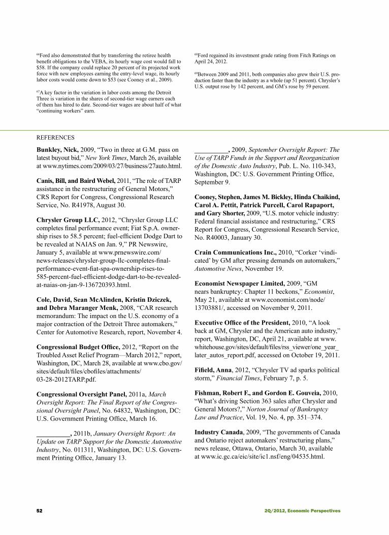
52 2Q/2012, Economic Perspectives
REFERENCES
Bunkley, Nick, 2009, “Two in three at G.M. pass on latest buyout bid,” New York Times, March 26, available at www.nytimes.com/2009/03/27/business/27auto.html.
Canis, Bill, and Baird Webel, 2011, “The role of TARP assistance in the restructuring of General Motors,” CRS Report for Congress, Congressional Research Service, No. R41978, August 30.
Chrysler Group LLC, 2012, “Chrysler Group LLC completes final performance event; Fiat S.p.A. owner-ship rises to 58.5 percent; fuel-efficient Dodge Dart to be revealed at NAIAS on Jan. 9,” PR Newswire, January 5, available at www.prnewswire.com/ news-releases/chrysler-group-llc-completes-final- performance-event-fiat-spa-ownership-rises-to-585-percent-fuel-efficient-dodge-dart-to-be-revealed-at-naias-on-jan-9-136720393.html.
Cole, David, Sean McAlinden, Kristin Dziczek, and Debra Maranger Menk, 2008, “CAR research memorandum: The impact on the U.S. economy of a major contraction of the Detroit Three automakers,” Center for Automotive Research, report, November 4.
Congressional Budget Office, 2012, “Report on the Troubled Asset Relief Program—March 2012,” report, Washington, DC, March 28, available at www.cbo.gov/ sites/default/files/cbofiles/attachments/ 03-28-2012TARP.pdf.
Congressional Oversight Panel, 2011a, March Oversight Report: The Final Report of the Congres-sional Oversight Panel, No. 64832, Washington, DC: U.S. Government Printing Office, March 16.
__________, 2011b, January Oversight Report: An Update on TARP Support for the Domestic Automotive Industry, No. 011311, Washington, DC: U.S. Govern-ment Printing Office, January 13.
__________, 2009, September Oversight Report: The Use of TARP Funds in the Support and Reorganization of the Domestic Auto Industry, Pub. L. No. 110-343, Washington, DC: U.S. Government Printing Office, September 9.
Cooney, Stephen, James M. Bickley, Hinda Chaikind, Carol A. Pettit, Patrick Purcell, Carol Rapaport, and Gary Shorter, 2009, “U.S. motor vehicle industry: Federal financial assistance and restructuring,” CRS Report for Congress, Congressional Research Service, No. R40003, January 30.
Crain Communications Inc., 2010, “Corker ‘vindi-cated’ by GM after pressing demands on automakers,” Automotive News, November 19.
Economist Newspaper Limited, 2009, “GM nears bankruptcy: Chapter 11 beckons,” Economist, May 21, available at www.economist.com/node/ 13703881/, accessed on November 9, 2011.
Executive Office of the President, 2010, “A look back at GM, Chrysler and the American auto industry,” report, Washington, DC, April 21, available at www.whitehouse.gov/sites/default/files/rss_viewer/one_year_later_autos_report.pdf, accessed on October 19, 2011.
Fifield, Anna, 2012, “Chrysler TV ad sparks political storm,” Financial Times, February 7, p. 5.
Fishman, Robert F., and Gordon E. Gouveia, 2010, “What’s driving Section 363 sales after Chrysler and General Motors?,” Norton Journal of Bankruptcy Law and Practice, Vol. 19, No. 4, pp. 351–374.
Industry Canada, 2009, “The governments of Canada and Ontario reject automakers’ restructuring plans,” news release, Ottawa, Ontario, March 30, available at www.ic.gc.ca/eic/site/ic1.nsf/eng/04535.html.
66Ford also demonstrated that by transferring the retiree health benefit obligations to the VEBA, its hourly wage cost would fall to $58. If the company could replace 20 percent of its projected work force with new employees earning the entry-level wage, its hourly labor costs would come down to $53 (see Cooney et al., 2009).
67A key factor in the variation in labor costs among the Detroit Three is variation in the shares of second-tier wage earners each of them has hired to date. Second-tier wages are about half of what “continuing workers” earn.
68Ford regained its investment grade rating from Fitch Ratings on April 24, 2012.
69Between 2009 and 2011, both companies also grew their U.S. pro-duction faster than the industry as a whole (up 51 percent). Chrysler’s U.S. output rose by 142 percent, and GM’s rose by 59 percent.

53Federal Reserve Bank of Chicago
Klier, Thomas H., 2009, “From tail fins to hybrids: How Detroit lost its dominance of the U.S. auto mar-ket,” Economic Perspectives, Federal Reserve Bank of Chicago, Vol. 33, Second Quarter, pp. 2–17.
Klier, Thomas, and James Rubenstein, 2011, “What role did regional policy play in addressing the US auto industry crisis?,” International Journal of Auto-motive Technology and Management, Vol. 11, No. 2, pp. 189–204.
Lassa, Todd, 2010, “The man who would be czar: Treasury Department’s chief auto industry advisor takes pragmatic approach to saving GM and Chrysler,” Motor Trend, March, available at www.motortrend.com/features/consumer/112_1005_ron_bloom_ interview/task_force_decision_process.html, accessed on May 31, 2011.
Li, Shanjun, Joshua Linn, and Elisheba Beia Spiller, 2011, “Evaluating ‘cash for clunkers’: Program effects on auto sales and the environment,” Resources for the Future, discussion paper, No. 10-39, August, revised October 2011.
Loomis, Carol, 2006, “The tragedy of General Motors,” Fortune, February 6, available at http://money.cnn.com/magazines/fortune/fortune_archive/2006/02/20/ 8369111/index.htm.
McAlinden, Sean, 2011, “Well, who won?,” presen-tation at the CAR (Center for Automotive Research) Breakfast Briefing, Detroit 3–UAW Labor Contract Negotiations, Schoolcraft Community College, Livonia, MI, November 29, available at www.cargroup.org/ assets/files/labor.pdf.
__________, 2008, “Well, who won? The future of automotive human resources in the United States,” presentation at the FACS Conference, Detroit, January 12.
Mian, Atif, and Amir Sufi, 2010, “The effects of fiscal stimulus: Evidence from the 2009 ‘cash for clunkers’ program,” National Bureau of Economic Research, working paper, No. 16351, September.
Muller, Joann, 2010, “UAW cashes in on GM IPO; pledges to help GM stay viable,” Forbes, November 18, available at www.forbes.com/sites/joannmuller/ 2010/11/18/uaw-cashes-in-on-gm-ipo-pledges-to- help-gm-stay-viable/.
O’Brien, Ellen, 2008, “What do the new auto industry VEBAs mean for current and future retirees?,” Insight on the Issues, AARP (American Association of Retired Persons) Public Policy Institute, No. I4, March, avail-able at http://assets.aarp.org/rgcenter/econ/i4_veba.pdf.
Office of the Special Inspector General for the Troubled Asset Relief Program (SIGTARP), 2012, Quarterly Report to Congress, Washington, DC, Jan-uary 26, available at www.sigtarp.gov/reports/congress/ 2012/January_26_2012_Report_to_Congress.pdf.
__________, 2010, “Factors affecting the decisions of General Motors and Chrysler to reduce their dealer-ship networks,” report, No. 10-008, Washington, DC, July 19, available at www.sigtarp.gov/reports/audit/ 2010/Factors%20Affecting%20the%20Decisions%20of%20General%20Motors%20and%20Chrysler%20to%20Reduce%20Their%20Dealership%20Networks %207_19_2010.pdf.
President of the United States of America, 2009, “Establishing a White House Council on Automotive Communities and Workers,” executive order, No. 13509, Federal Register, Vol. 74, No. 122, June 26, available at www.gpo.gov/fdsys/pkg/FR-2009-06-26/pdf/E9-15368.pdf.
Rattner, Steven, 2010a, Overhaul—An Insider’s Account of the Obama Administration’s Emergency Rescue of the Auto Industry, New York: Houghton Mifflin Harcourt.
__________, 2010b, “Reflections on the auto restructur-ings,” speech at the Federal Reserve Bank of Chicago conference, After the Perfect Storm: Competitive Forces Shaping the Auto Industry, Detroit, May 10–11, available at www.chicagofed.org/digital_assets/others/ events/2010/automotive_perfect_storm/rattner.pdf.
Schwartz, Arthur R., 2011a, “A look back and a look forward,” presentation at the CAR (Center for Automotive Research) Breakfast Briefing, Detroit 3– UAW Labor Contract Negotiations, Schoolcraft Community College, Livonia, MI, November 29, available at www.cargroup.org/assets/files/labor.pdf.
__________, 2011b, “Setting the stage: 2005–2009 UAW–Detroit Three talks,” presentation at the 2011 CAR (Center for Automotive Research) Management Briefing Seminars, Bargaining for a Competitive Future: The 2011 Negotiations between the UAW and the Detroit Three, Grand Traverse Resort & Spa, Traverse City, MI, August 3, available at http://mbs.cargroup.org/2011/Dziczek&Schwartz.pdf.

54 2Q/2012, Economic Perspectives
Scott, Robert E., 2008, “When giants fall: Shutdown of one or more U.S. automakers could eliminate up to 3.3 million U.S. jobs,” Economic Policy Institute, briefing paper, No. 227, December 3.
Shiell, Leslie, and Robin Somerville, with com-mentary by Jim Stanford, 2012, “Bailouts and subsidies: The economics of assisting the automotive sector in Canada,” IRPP Study, Institute for Research on Public Policy, No. 28, March, available at www.irpp.org/pubs/IRPPstudy/IRPP_Study_no28.pdf.
Snavely, Brent, 2012, “Chrysler withdraws applica-tion for Department of Energy loan,” Detroit Free Press, February 16.
Spector, Mike, 2012, “Chrysler got legal shield in Chapter 11,” Wall Street Journal, April 4, available at http://online.wsj.com/article/SB10001424052702304450004577277802983129074.html?KEYWORDS =mike+spector.
Strauss, William A., and Emily A. Engel, 2009, “Economy to turn the corner in 2010,” Chicago Fed Letter, Federal Reserve Bank of Chicago, No. 265a, August.
U.S. Department of the Treasury, 2010, “Troubled Assets Relief Program (TARP) monthly 105(a) report—June 2010,” report, Washington, DC, July 12, avail-able at www.treasury.gov/initiatives/financial- stability/briefing-room/reports/105/Documents105/June%202010%20105(a)%20Report_Final.pdf.
U.S. Department of the Treasury, Office of Financial Stability, 2012, “TARP transaction report,” report, Washington, DC, April 2, available at www.treasury.gov/initiatives/financial-stability/briefing-room/ reports/tarp-transactions/Pages/default.aspx.
Vlasic, Bill, 2011, Once Upon a Car: The Fall and Resurrection of America’s Big Three Auto Makers—GM, Ford, and Chrysler, New York: HarperCollins.
Webel, Baird, and Bill Canis, 2011, “TARP assistance for Chrysler: Restructuring and repayment issues,” CRS Report for Congress, Congressional Research Service, No. R41940, July 27.
White House, 2010, “Annual report of the White House Council on Automotive Communities and Workers,” report, Washington, DC, May.
__________, 2009a, “GM February 17 plan: Viability determination,” report, Washington, DC, March 30, available at www.whitehouse.gov/assets/documents/GM_Viability_Assessment.pdf.
__________, 2009b, “Obama Administration new path to viability for GM & Chrysler,” fact sheet, Washington, DC, March 30, available at www.whitehouse.gov/ assets/documents/Fact_Sheet_GM_Chrysler_FIN.pdf.
__________, 2008, “Fact sheet: Financing assistance to facilitate the restructuring of auto manufacturers to attain financial viability,” Washington, DC, December 19, available at http://georgewbush-whitehouse.archives. gov/news/releases/2008/12/20081219-6.html.
White House, Office of the Press Secretary, 2012, remarks by the President in State of the Union Address in the United States Capitol, Washington, DC, Janu-ary 24, available at www.whitehouse.gov/the-press-office/2012/01/24/remarks-president-state-union-address.
Wilson, Amy, 2012, “Bush defends GM, Chrysler loans,” Automotive News, February 6, available at www.autonews.com/apps/pbcs.dll/article?AID=/ 20120206/RETAIL06/120209848.
York, Jerry, 2006, “Full text of Jerry York’s speech,” Financial Times, January 10, available by subscription at www.ft.com/intl/cms/s/0/638427aa-821f-11da- aea0-0000779e2340.html#axzz1nFQQdenQ.
Zandi, Mark, 2008, “The state of the domestic auto industry: Part II,” testimony before the U.S. Senate Committee on Banking, Housing, and Urban Affairs, Washington, DC, December 4.

55Federal Reserve Bank of Chicago
No-arbitrage restrictions and the U.S. Treasury market
Andrea Ajello, Luca Benzoni, and Olena Chyruk
Introduction and summary
The secondary U.S. Treasury market is among the largest, most liquid, and most important financial markets world-wide. Daily trading volume in 2011 averaged $567.8 billion, more than tenfold the volume at the New York Stock Exchange (NYSE).1 The market is open around the clock, with trading involving both U.S. and inter-national participants. Competition among dealers and brokers typically results in low bid–ask spreads, low brokerage fees, and fast order execution (for example, Fleming, 1997). Such features make the market very liquid across a wide spectrum of maturities.
Arbitrage is the practice of taking advantage of a price differential between securities that pay out similar cash flows (we provide a more rigorous definition at the beginning of the next section). This concept has im-mediate application in the U.S. Treasury market. For instance, consider two alternative investment strategies. The first entails purchasing a ten-year Treasury note. The second involves an investment of the same amount in a three-month Treasury bill that we repeatedly roll over at maturity into a newly issued three-month bill. For markets to clear, and absent market frictions, the price of the ten-year note needs to reflect investors’ expectations about the future path of the three-month Treasury rate during the next ten years. These expecta-tions involve an adjustment to compensate risk-averse investors for bearing the risk that the price of the ten-year note will fluctuate during the holding period. If Treasury yields were to violate this condition, in a well-functioning capital market arbitrage trading would move funds across assets until prices adjust to balance out profit opportunities. By the same argument, yields on Treasury securities with various maturities will satisfy similar cross-sectional restrictions.
The Federal Reserve exploits the linkage across the term structure of bond yields to influence the availability and cost of money and credit in the economy.
For instance, the Federal Open Market Committee (FOMC) uses open market operations to achieve a desired target rate in the federal funds market, where depository institutions lend balances at the Federal Reserve to other depository institutions overnight.2 Changes in the federal funds rate trigger a chain of events that affect other short-term interest rates,
Andrea Ajello is an economist in the Division of Monetary Affairs at the Board of Governors of the Federal Reserve System. Luca Benzoni is a senior financial economist and Olena Chyruk is a senior research analyst in the Economic Research Department at the Federal Reserve Bank of Chicago. The authors are grateful to Gene Amromin, Gadi Barlevy, Marco Bassetto, Jarda Borovička, Charlie Evans, Robert Goldstein, Alejandro Justiniano, Spencer Krane, David Marshall, Richard Porter, Robert Steigerwald, an anonymous referee, and seminar participants at the Federal Reserve Bank of Chicago for helpful comments and suggestions.
© 2012 Federal Reserve Bank of Chicago Economic Perspectives is published by the Economic Research Department of the Federal Reserve Bank of Chicago. The views expressed are the authors’ and do not necessarily reflect the views of the Federal Reserve Bank of Chicago or the Federal Reserve System.Charles L. Evans, President; Daniel G. Sullivan, Executive Vice President and Director of Research; Spencer Krane, Senior Vice President and Economic Advisor; David Marshall, Senior Vice President, financial markets group; Daniel Aaronson, Vice President, microeconomic policy research; Jonas D. M. Fisher, Vice President, macroeconomic policy research; Richard Heckinger, Vice President, markets team; Anna L. Paulson, Vice President, finance team; William A. Testa, Vice President, regional programs; Richard D. Porter, Vice President and Economics Editor; Helen Koshy and Han Y. Choi, Editors; Rita Molloy and Julia Baker, Production Editors; Sheila A. Mangler, Editorial Assistant.Economic Perspectives articles may be reproduced in whole or in part, provided the articles are not reproduced or distributed for commercial gain and provided the source is appropriately credited. Prior written permission must be obtained for any other reproduc-tion, distribution, republication, or creation of derivative works of Economic Perspectives articles. To request permission, please contact Helen Koshy, senior editor, at 312-322-5830 or email [email protected].
ISSN 0164-0682

56 2Q/2012, Economic Perspectives
foreign exchange rates, and the amount of money and credit. Most people, however, care especially about the cost of long-term credit—many firms rely on long-term debt to fund capital investment, and households take on long-term loans to buy their homes and cars. These observations underscore the importance of term structure models that help us gauge the effect of monetary policy actions (which typically impact the short end of the term structure) on long-term yields and, ultimately, a range of economic variables, including employment, output, and the prices of goods and services.
In this article, we discuss the pricing of U.S. Treasury securities via no-arbitrage arguments. We initially define what an arbitrage is and provide an intuitive one-period example that shows how to con-struct an arbitrage investment strategy in a frictionless capital market. We argue that absent transaction costs, information asymmetries, and other market imperfec-tions, investors will trade away arbitrage opportunities. This will discipline the movement in prices of assets that are exposed to the same source of risk. We then formalize this intuition in the classical no-arbitrage term structure model of Vasicek (1977). We show that no-arbitrage arguments restrict the amount of return that investors demand in compensation for bearing a unit of risk (the so-called market price of risk) to be identical across the cross section of bonds. Exploiting this condition, Vasicek obtains a bond pricing formula that expresses the price of bonds of various maturities as a function of the spot interest rate, the market price of risk, and other model parameters.
This discussion also highlights the limitations of the Vasicek model. First, Vasicek assumes the market price of risk to be exogenous—his approach is silent about the economic forces that determine the amount of compensation investors require to bear risk. To clarify this link, we recast his model in a general equilibrium setting. This analysis shows that the market price of risk depends in fact on economic fundamentals such as the investors’ attitude toward risk and the volatility of the growth rate in aggregate consumption.
Second, in the Vasicek model a single variable, the spot interest rate, explains the fluctuations in the entire cross section of Treasury yields. One implication of this assumption is that bond yields and their changes are perfectly correlated. Correlations in pairs of yields with different maturities are positive and high in the data; however, they decrease considerably as the time to maturity of bonds becomes further apart. This feature suggests that additional factors might drive the U.S. Treasury yield curve and motivates a vast literature that extends the class of no-arbitrage term structure models to include multiple factors. We present an overview
of this class of models, with an emphasis on the spec-ifications that, similar to Vasicek’s model, allow for tractable bond pricing formulas (the so-called affine dynamic term structure models).
Third, the predictions of no-arbitrage models hinge on the critical assumption that markets are “perfect.” In order to take advantage of arbitrage opportunities, investors require access to capital. To trade away price misalignments, they need to be able to exchange secu-rities at minimal cost based on information that is available to, and readily interpretable by, all investors. Clearly, no market satisfies all these conditions, and frictions typically become more severe during times of market stress. In extreme cases, markets could be-come segmented and arbitrage opportunities remain unexploited because of balance-sheet capacity limita-tions or because of higher-than-normal uncertainty and risk aversion. These conditions could reduce the effec-tiveness of no-arbitrage pricing arguments, possibly to a point where prices deviate from fundamental values.
Most of the time, frictions in the U.S. Treasury market are small. For instance, bid–ask spreads and other transaction costs are usually very low, and investors can trade securities with ease (for example, Fleming, 1997). Financial and economic crises typically do not impair these conditions. In fact, a flight to quality and/or liquidity can increase the demand for U.S. govern-ment debt, especially the most recently issued short-maturity nominal Treasury securities. This happened, in particular, during the recent financial crisis, when investors displayed a desire to hold only the safest and most liquid assets (for example, Gorton and Metrick, 2011; and Krishnamurthy, 2010). Nonetheless, govern-ment debt markets can exhibit some degree of segmen-tation because of the preferences by some investor clienteles (for example, pension funds, insurance com-panies, and other institutional investors) to hold secu-rities that have specific maturities. So-called preferred habitat theories argue that these preferences could limit the substitutability of short- and long-term Treasury securities, distorting their relative pricing; capital con-straints and risk aversion might prevent arbitrageurs from eliminating such profit opportunities. In the last part of the article, we expand on this discussion, focus-ing on the literature that studies limits to arbitrage in the government debt market.
Fourth, the dynamic term structure models that we review here typically rely on latent factors (or lin-ear combinations of yields) to explain the variation in Treasury yields. Thus, this framework does not explain how bond yields respond to macroeconomic shocks, as these factors are void of immediate economic in-terpretation. Similarly, these models are silent about
57Federal Reserve Bank of Chicago
the effect of monetary policy on economic variables, such as unemployment, gross domestic product (GDP) growth, and consumer prices. In response to these shortcomings, several recent studies explore the linkage between U.S. Treasury securities and the macroeconomy in no-arbitrage term structure models. We touch upon these issues at the very end, and postpone further dis-cussion to the future.
No-arbitrage pricing in a one-period example
An arbitrage is an investment strategy that entails a nonpositive initial cost to generate a nonnegative cash flow that is positive with positive probability at some future date. Arbitrage opportunities should not exist in a frictionless market. Without transaction costs, in-formation asymmetries, and other market imperfections, investors would immediately take advantage of any arbitrage opportunity. By doing so, they will close any misalignment in prices: Excess demand will push up the cost of securities that are relatively undervalued, and excess supply will lower the price of overvalued assets. Thus, no-arbitrage trading guarantees that securities are priced to reflect their future cash flow stream.
As a simple illustration of this concept, consider the case of an investor who trades in two assets at prices P1(t) and P2(t) on date t. The two securities do not pay dividends and are exposed to the same source of risk, so that their returns from t to t + 1 are described by the model
1 1 1 1 2) ( )( )
( ) ( )( )
, , .∆P tP t
P t P tP t
t ii
i
i i
ii i≡
+ −= + +( ) =µ εΣ
Here, µi denotes the constant expected rate of return on security i during the unit interval, while the sto-chastic term (Σiε) is a mean zero innovation in the rate of return, with constant variance Σ
i2. Being subject to
the same shock ɛ, the returns on the two assets by con-struction are perfectly correlated. Thus, the investor can exploit the co-movement in the two securities to eliminate risk from her portfolio. Suppose that she sells short W1 worth of the first security’s shares and places a wealth amount W2 in the second security. At time t, the portfolio is worth W ≡ W2 – W1 in wealth. During the interval from t to t + 1, the change in wealth is determined by the rate of return on the two securities over that interval,
2) ∆∆
∆
W t W t W t W t P tP t
W t P tP t
( ) ( ) ( ) ( ) ( )( )
( ) ( )( )
.
≡ + − =
−
1 22
2
11
1
Substituting the expression for the rate of return P tP ti
i
( )( )
Δ and rearranging the terms, we simplify equation 2 to
3) ∆W t W t W t
W t W t t
( ) ( ( ) ( ) )
( ( ) ( ) ) ( ).
= −
+ − +
2 2 1 1
2 2 1 1 1
µ µ
εΣ Σ
An appropriate choice of W2 and W1 eliminates uncer-tainty in the strategy’s return. In particular, if the in-vestor sets W1 = W Σ2 /(Σ1– Σ2) and W2 = W Σ1/(Σ1– Σ2), the second term in equation 3 vanishes and the rate of return on invested wealth over the interval from t to t + 1 simplifies to
4 2 1 1 2
1 2
) ( )( )
.∆ Σ ΣΣ Σ
W tW t
=−−
µ µ
At this point, we want to rule out arbitrage opportunities. To this end, we need to have the return on wealth in equation 4 equal the risk-free rate, r, which we assume to be constant in this example. Thus, we have the fol-lowing condition:
5 2 1 1 2
1 2
) .µ µΣ ΣΣ Σ
−−
= r
Rearranging terms in equation 5, we obtain the market clearing condition that links the expected return on the two securities, in excess of the risk-free rate, per unit of return standard deviation:
6 2
2
1
1
) .µ µ−=
−r rΣ Σ
We denote the common value for this ratio with λ:
7 1 2) , , .λµ
=−
=i
i
r iΣ
The ratio λ measures the market price of risk; that is, it quantifies the amount of return that investors demand in compensation for a unit of risk that they bear. To rule out arbitrage opportunities, we must have the coefficients µi and Σi that determine the returns on securities i = 1 and 2 in equation 1 satisfy the condi-tion in equation 7. Intuitively, this restriction ties the price of the first security to that of the second security.

58 2Q/2012, Economic Perspectives
In the next section, we explain how these prices are tied together.
The Vasicek model
Here, we follow the Vasicek (1977) framework closely. We let the length of the time interval shrink to zero and recast the example from the previous section in continuous time. This simplifies the exposition con-siderably and clearly conveys the intuition for the results.
Assume that the spot risk-free rate, r, in a friction-less market follows a mean-reverting diffusion process
8) ( ) ,dr r dt dZ= − +κ θ Σ
where Z is a standard Brownian motion. Equation 8 is a continuous-time analogue to the return process in equation 1. The left-hand side has the instantaneous change in the spot interest rate, dr = r(t + dt) – r(t). Similar to equation 1, the right-hand side of equation 8 is the sum of the expected change in r, conditional on the realization of the time t spot rate, as well as a ran-dom shock. In particular, the term κ(θ – r) describes the conditionally deterministic component of the spot rate evolution, with the coefficient κ > 0 control-ling the speed of mean reversion of the process r toward its long-run mean θ. The Brownian shock dZ = Z(t + dt) – Z(t) has Gaussian distribution with mean zero and variance dt, N(0, dt). It takes place of the mean zero shock ɛ over the discrete time interval from t to t + 1 in equation 1, where Var(ɛ) = Δt = 1. The coefficient Σ2 represents the constant instanta-neous variance of the stochastic fluctuations of the spot rate. Equation 8 satisfies the affine restrictions of Duffie and Kan (1996); that is, the drift term κ(θ – r) is a linear-plus-constant function of the spot rate r, and the quadratic variation of the process is the constant Σ2. These restrictions help us to obtain a closed-form bond pricing formula, which we derive next.
In the Vasicek model, the spot rate r summarizes the uncertainty in the economy. In particular, the time t price of a zero-coupon bond with maturity date T is determined by the assessment, at time t, of the evolu-tion of the spot rate rs , with t ≤ s ≤ T. Itô’s formula gives then the dynamics for the bond price Pt = P(rt , τ), where τ = T – t:
9 12
2
22) ( )
( , )
dP Pt
Pr
r Pr
dt
PrdZ
P r dt
=∂∂
+∂∂
− +∂∂
+∂∂
= +
κ θ
µ τ
Σ
Σ
PP r dZσ τ( , ) ,
where we have suppressed time t subscripts and defined
10 1 12
1
2
22) ( , ) ( ) ,
( , )
µ τ κ θ
σ τ
rP
Pt
Pr
r Pr
rPPr
≡∂∂
+∂∂
− +∂∂
≡∂∂
Σ
ΣΣ .
Following steps similar to those of the previous example, we consider an investor who sells short W1 worth of the bond with maturity T1 and who places wealth W2 in the bond with maturity T2 . This strategy is worth W ≡ W2 – W1 in wealth at time t, which evolves according to
11 22
21
1
1
) ( , )( , )
( , )( , )
,
dW W dP rP r
W dP rP r
dt dZW W
= −
= +
ττ
ττ
µ σ
where µW = W2 µ(r, τ2) – W1 µ(r, τ1) and σW = W2 σ (r, τ2) – W1 σ (r, τ1). The investor can choose W1 and W2 to dynamically hedge her portfolio. In particular, setting
12 12
1 2
21
1 2
) ( , )( , ) ( , )
,
( , )( , ) ( , )
W r Wr r
W r Wr r
=−
=−
σ τσ τ σ τ
σ τσ τ σ τ
eliminates risk from her investment; that is, σW = 0 and the second term in the right-hand side of equation 11 vanishes. Thus, the position is insulated from the stochas-tic shock dZ, and the instantaneous rate of return on invested wealth simplifies to
13 1 2 2 1
1 2
) ( , ) ( , ) ( , ) ( , )( , ) ( , )
.dWW
r r r rr r
dt=−−
σ τ µ τ σ τ µ τσ τ σ τ
To avoid arbitrage opportunities, we need to have the growth rate in wealth to equal the risk-free rate,
14 1 2 2 1
1 2
) ( , ) ( , ) ( , ) ( , )( , ) ( , )
.σ τ µ τ σ τ µ τσ τ σ τ
r r r rr r
r−−
=

59Federal Reserve Bank of Chicago
Rearranging terms, we obtain a condition similar to equation 6:
15 1
1
2
2
) ( , )( , )
( , )( , )
.µ τσ τ
µ τσ τ
r rr
r rr
−=
−
That is, the market price of risk λ is a function of the sole state variable of the economy, r, and is indepen-dent of the bond time to maturity τ,
16 0) ( ) ( , )( , )
, .λµ τ
σ ττr r r
r=
−∀ ≥
To obtain a closed-form bond pricing formula, Vasicek assumes the market price of risk is constant; that is,
17 0) .( )λ λr =
Substituting the expression for µ(r, τ) and σ(r, τ) from equation 10 in equation 16 yields a partial dif-ferential equation for the bond price P:
18 12
0
02
2
2) ( ( ) )
, ,
∂∂
+ − −∂∂
+∂∂
− = ≥
Pt
r Pr
Pr
rP T t
κ θ λΣ Σ
with terminal condition P(r, τ = 0) =1. The solution to this equation is exponentially affine in the spot rate r; that is, there are functions A( )τ and B( )τ of time to maturity τ such that
19) ( ) exp ( ) ( )P r A B r, = + .τ τ τ{ }
Thus, we obtain a closed-form expression for the term structure of interest rates. In particular, the yield y on the bond with maturity date T is affine in the spot rate r:
20) ( ) ( ) ( ) ,y r A B r, = +τ τ τ
where A A( ) ( )τ τ τ= − / and B B( ) ( ) .τ τ τ= − /
The determinants of the market price of risk
The Vasicek (1977) bond pricing formula hinges on the principle that absent arbitrage opportunities, the return on a locally risk-free portfolio of bonds must equal the risk-free rate. This approach is silent about the sources of the market price of risk λ, and it takes the spot risk-free rate dynamics in equation 8 as given. Here, we show that the Vasicek bond pricing formula is consistent with the solution of the intertemporal con-sumption decision problem of a representative investor. While we arrive at the same pricing formula, this gen-eral equilibrium approach restricts the properties of the market price of risk and the instantaneous risk-free rate r, which become functions of the investor’s attitude toward risk and the parameters that govern the aggre-gate dividend process. These results are well known in the literature (for example, Cox, Ingersoll, and Ross, 1985). The discussion in this section follows Goldstein and Zapatero (1996) and Cochrane (2005) closely.
Consider a security with ex-dividend price p that represents a claim to the aggregate output of the economy, which is paid out to the holder of the secu-rity in the form of a dividend D. We assume that the security generates an ex-dividend return
21) dpp
dt dZt
tt t t= + ,µ σ
where μt is the ex-dividend expected rate of return on security p, σt
2 is the instantaneous variance of the stochastic fluctuation in security p’s return, and Z is a standard Brownian motion. The quantities μt and σt are endogenous to the model and will be determined in equilibrium. In contrast, the aggregate dividend is exogenously given by
22)
( )
dDD
dt dZ
d dt dZ
t
tt t
t t t
= +
= − + .
α ξ
α κ α α ν
,
Consider now an infinitely lived representative investor who trades in the security p and maximizes her lifetime utility of consumption,
23) ( ) ( )( )U c s t E e u c dss t t
s ts{ }, ≥ =
.
∞ − −∫ δ
Cochrane (2005) shows that the first-order condition for this problem generates the basic pricing equation,

60 2Q/2012, Economic Perspectives
240
) ( ) ( )p u c E e u c D dst t ts
t s t s′ = ′ ,∞ −
+ +∫ δ
which equates the marginal cost of acquiring the security today at price pt to the marginal benefit generated by its future dividend stream. Defining the discount factor as Λ t
tte u c≡ ′−δ ( ) , we can rewrite equation 24 as:
250
) p E D dst t t t s t sΛ Λ= .∞
+ +∫
Consider now a strategy that buys security p at time t and sells it at time t + Δ . Equation 25 then yields
260
) [ ]p E D ds E pt t t t s t s t t tΛ Λ Λ= + .∆
+ + +∆ +∆∫
For small Δ → 0, this can be approximated by:
27 0) [ ( )]= + .Λ Λt t t t tD dt E d p
Itô’s lemma yields d p p d dp dp dt t t t t t t t( ) ,Λ Λ Λ Λ= + + so that equation 27 becomes:
28 0) = + + +
.
Dpdt E d dp
pd dp
pt
tt
t
t
t
t
t
t
t
t
ΛΛ
ΛΛ
Using equation 25 to price the (instantaneous) risk-free zero-coupon bond, we obtain an expression for the spot risk-free rate,
29) rdt E dt t
t
t
= −
.
ΛΛ
Then, rearranging equation 28, we obtain an equilibri-um condition for the expected rate of return on secu-rity p, μt:
30) E dpp
Dpdt rdt E d dp
ptt
t
dt
t
tt t
t
t
t
t
t
+ − = −
.
µ��� ��
ΛΛ
Assume now that the investor has the power utility function u ct
ct( ) =−
−
1
1
γ
γ with the coefficient of risk aversion γ. By the definition of Λt , the stochastic discount factor dynamics are
31 12
12
) ( )d dt dcc
dcc
t
t
t
t
t
t
ΛΛ
= − − + +
,δ γ γ γ
so that equation 30 becomes:
32) .E dpp
Dpdt rdt E dc
cdppt
t
t
t
tt t
t
t
t
t
+ − =
γ
Equation 32 says that the expected excess cum-dividend return on security p is proportional to the risk aversion coefficient γ. Thus, more-risk-averse investors demand a higher risk premium to hold p. Moreover, the risk premium on p depends on the correlation between aggregate consumption growth and the return on p,Et
dccdpp
t
t
t
t . Thus, an investor will require a positive
risk premium to hold a security that generates a high return when consumption growth is high, that is, whenEt
dccdpp
t
t
t
t > 0. This is intuitive, as such security
generates, in expectation, a low payoff when consump-tion is low. This property makes the security less valu-able to the investor, who is risk averse and wishes to smooth her consumption profile.
Note that in equilibrium, aggregate consumption equals the aggregate dividend, and thus it has dynam-ics identical to those given in equation 22. Substitut-ing the endowment growth rate in equation 29 yields an expression for the equilibrium risk-free rate:
33 12
1 2) ( )rt t= + − + .δ γα γ γ ξ
Itô’s lemma gives us the spot rate dynamics
34) ( )dr r dt dZt t t= − + ,κ θ Σ
where we have defined the coefficients θ γα δ≡ +− +1
221γ γ ξ( ) and Σ ≡ γν. Equation 34 is identical to the
spot rate dynamics in equation 8, as in the Vasicek (1977) model. However, via equilibrium arguments we have established a linkage between the coeffi-cients κ, θ, and Σ and economic fundamentals (that is, the coefficients κ, ᾱ, δ, ξ, and ν that govern the endowment dynamics in equation 22 and the risk aversion parameter γ).
To obtain a formula for the price P of a zero-coupon bond with maturity date T, it is useful to compute the spot rate dynamics under the risk-adjusted probability measure Q (Harrison and Kreps, 1979). With the help of equation 32, we obtain:
35) ( )dr r dt dZtQ
t tQ= − + ,κ θ Σ
where we have defined θ θ γξκ
Q ≡ − Σ and dZ dZtQ
t≡ + γ ξdt. Then, we have

61Federal Reserve Bank of Chicago
label
FIguRE 1
U.S. Treasury yields
Notes: The plot depicts the time series of monthly U.S. Treasury yields with one-, four-, 12-, 20-, 40-, and 80-quarter (Q) maturities. The one-quarter yield is from the Fama CRSP Treasury bill files. The yields with a maturity greater than one quarter are zero-coupon yields interpolated from daily constant-maturity par yields computed by the U.S. Department of the Treasury and distributed by the Board of Governors of the Federal Reserve System in the H.15 statistical release. The sample period is January 1962–December 2010.Sources: Authors’ calculations based on data from the University of Chicago Booth School of Business, Center for Research in Security Prices (CRSP), Fama CRSP Treasury bill files; and Board of Governors of the Federal Reserve System, H.15 statistical release.
1962 ’65 ’68 ’71 ’74 ’77 ’80 ’83 ’95 2001’98’92’89’860
2
4
6
8
10
12
14
16
18
1Q4Q
12Q20Q
40Q80Q
’04 ’10’07
percent per year
36) ( )P t T E etQ r du
t
Tu, = ∫
,
−
where the conditional expectation EtQ[ ]⋅ is computed
under the risk-adjusted measure Q.The spot rate in equation 35 is a continuous Markov
process. Thus, the evolution of ru over the interval (t, T ), given the history up to time t, depends only on rt. Equation 36 then implies that the bond price is a function of rt , P(t, rt , T ), and by Itô’s lemma we obtain:
37 12
2
22) ( )dP P
tPr
r Pr
dt PrdZ=
∂∂
+∂∂
− +∂∂
+∂∂
.
κ θ Σ Σ
Moreover, we can apply equation 32 to determine the expected rate of return on the zero-coupon bond, in excess of the spot rate:
38) E dPP
rdt E dccdPPt t
− =
.γ
Combining equations 37 and 38, we derive the funda-mental differential equation for bonds:
39 12
00
2
22) ( )∂
∂− −
+∂∂
+∂∂
− = ,≡
Pr
r Pr
PtrPκ θ γ ξ
λ
Σ Σ
where ξ is the diffusion coefficient of the aggregate endowment process given in equation 22. Equation 39 is identical to the partial differential equation of the Vasicek model (equation 18) with the restriction λ0 = γξ. Consequently, assumptions about investors’ preferences and their endowment pin down the speci-fication of the market price of risk. Specifically, λ0 is higher when the investor is more risk averse, γ↑, and when consumption growth is more volatile, ξ↑.
Multifactor dynamic term structure modelsIn the Vasicek (1977) model, a single factor, the
spot rate r, explains the fluctuations in the entire term structure of interest rates. One implication of this assump-tion is that bond yields and their changes are perfectly correlated. A cursory glance at figure 1 shows that there are co-movements in yields with different maturities,

62 2Q/2012, Economic Perspectives
TaBlE 1
Pairwise correlations in U.S. Treasury yield series
1Q 4Q 12Q 20Q 40Q 80Q 1Q 4Q 12Q 20Q 40Q 80Q
A. Monthly series
1Q 1.00 1.00 4Q 0.99 1.00 0.71 1.00 12Q 0.95 0.98 1.00 0.63 0.92 1.00 20Q 0.93 0.96 0.99 1.00 0.56 0.86 0.97 1.00 40Q 0.88 0.92 0.97 0.99 1.00 0.47 0.73 0.87 0.93 1.00 80Q 0.82 0.86 0.93 0.96 0.98 1.00 0.36 0.58 0.71 0.79 0.88 1.00
B. Quarterly series
1Q 1.00 1.00 4Q 0.99 1.00 0.90 1.00 12Q 0.96 0.98 1.00 0.78 0.94 1.00 20Q 0.93 0.96 0.99 1.00 0.69 0.88 0.98 1.00 40Q 0.88 0.92 0.97 0.99 1.00 0.58 0.77 0.91 0.96 1.00 80Q 0.82 0.86 0.93 0.96 0.98 1.00 0.43 0.60 0.75 0.82 0.90 1.00
Notes: Both panels show the pairwise correlations between U.S. Treasury yields with various maturities. Panel A reports the correlations computed on monthly yields (left) and changes in monthly yields (right). Panel B shows the results for quarterly yields (left) and changes in quarterly yields (right). The data series consist of yields with one-, four-, 12-, 20-, 40-, and 80-quarter (Q) maturities. The one-quarter yield is from the Fama CRSP Treasury bill files. The yields with a maturity greater than one quarter are zero-coupon yields interpolated from daily constant-maturity par yields computed by the U.S. Department of the Treasury and distributed by the Board of Governors of the Federal Reserve System in the H.15 statistical release. The sample period is January 1962–December 2010.Sources: Authors’ calculations based on data from the University of Chicago Booth School of Business, Center for Research in Security Prices (CRSP), Fama CRSP Treasury bill files; and Board of Governors of the Federal Reserve System, H.15 statistical release.
TaBlE 2
Principal component analysis
Percentage of Total percentage of variance explained variance explained
monthly quarterly monthly quarterly
PC1 95.19 95.34 95.19 95.34PC2 4.25 4.17 99.44 99.51PC3 0.41 0.37 99.85 99.88PC4 0.11 0.08 99.96 99.96PC5 0.04 0.03 99.99 99.99PC6 0.01 0.01 100.00 100.00
Notes: The table reports the percentage of the yields’ variation explained by the principal components, PCj , j = 1, …, 6, extracted from the panel of yields with one-, four-, 12-, 20-, 40-, and 80-quarter maturities sampled at the monthly and quarterly frequencies. The one-quarter yield is from the Fama CRSP Treasury bill files. The yields with a maturity greater than one quarter are zero-coupon yields interpolated from daily constant-maturity par yields computed by the U.S. Department of the Treasury and distributed by the Board of Governors of the Federal Reserve System in the H.15 statistical release. The sample period is January 1962–December 2010.Sources: Authors’ calculations based on data from the University of Chicago Booth School of Business, Center for Research in Security Prices (CRSP), Fama CRSP Treasury bill files; and Board of Governors of the Federal Reserve System, H.15 statistical release.
but such correlations are far from perfect. This is evident in table 1, which reports pairwise correlations in yields and their changes, corr y y
i j( )τ τ, and
corr y yi j
( ),∆ ,∆τ τ for maturity pairs τi and τj ranging
from one quarter to 20 years. While the correlations in both the monthly (panel A) and quarterly (panel B) series are positive, they decrease considerably as the time to maturity in the pairs of bonds becomes further apart. This feature suggests that additional factors might drive the term structure of U.S. Treasury yields.
The evidence in table 2 lends additional support to this conclusion. It shows the percentage of the yields’ variation explained by the principal components (PCs) extracted from the panel of bond yields with one-, four-, 12-, 20-, 40-, and 80-quarter maturi-ties. The first principal component has the highest explanatory power, accounting for more than 95 percent of the variation in monthly and
quarterly yields. The second and third components account for virtually all of the residual variation in yields. This is well known in the term structure litera-ture; for instance, Litterman and Scheinkman (1991)
corr y ,yi
( τ τ j) corr y ,
i j( )∆ ∆τ τy

63Federal Reserve Bank of Chicago
FIguRE 2
U.S. Treasury yields’ principal components coefficients
Notes: The plot depicts the coefficients Bτ that multiply the yields to form the U.S. Treasury yields’ first three principal components, PCj , j = 1, 2, and 3, as a function of the yields’ maturity τ. The authors compute the principal components using monthly yields series with one-, four-, 12-, 20-, 40-, and 80-quarter maturities. The one-quarter yield is from the Fama CRSP Treasury bill files. The yields with a maturity greater than one quarter are zero-coupon yields interpolated from daily constant-maturity par yields computed by the U.S. Department of the Treasury and distributed by the Board of Governors of the Federal Reserve System in the H.15 statistical release. The sample period is January 1962–December 2010.Sources: Authors’ calculations based on data from the University of Chicago Booth School of Business, Center for Research in Security Prices (CRSP), Fama CRSP Treasury bill files; and Board of Governors of the Federal Reserve System, H.15 statistical release.
0 10 20 30 40 50 60 70 80−0.8
−0.6
−0.4
−0.2
0
0.2
0.4
0.6
1PCB
2PCB 3PCB
τ
τ τ
maturity in quarters
show that the variation in U.S. Treasury rates is best captured by three factors, interpreted as changes in “level,” “slope,” and “curvature” of the yield curve.
Figure 2 clarifies this interpretation. The yields’ PCs are an orthogonal linear transformation of the yields’ series; they are constructed so that each com-ponent explains the highest fraction of residual vari-ance in the original series and is orthogonal to the preceding PCs. Figure 2 shows the coefficients in the vector Bτ that multiply the yields to form the first three principal components, PCj , j = 1, 2, and 3, as a function of the yields’ maturity τ. The coefficients as-sociated with the first PC are roughly the same across the yields’ maturities. This suggests that PC1 is a proxy for a level factor, that is, shocks to that factor result in a parallel shift in yields across maturities. Consistent with this view, the correlation between PC1 and yτ, τ ∈{1, 4, 12, 20, 40, and 80 quarters} rang-es from 93.6 to 99.7 percent in monthly data; we find similar values in the quarterly series. This is also evi-dent in figure 3, which shows that the pattern in PC1
resembles the shape of the yields in figure 1.
In contrast, the coefficients of the second PC are increasing in yields’ maturity τ, while those of the third one are U-shaped, as shown in figure 2. Thus, as in Litterman and Scheinkman (1991), PC2 is a proxy for a slope factor (positive shocks to this factor are associated with lower short-maturity yields and higher long- maturity yields), while PC3 is a proxy for curvature. Indeed, the correlation between PC2 and a measure of the term structure slope, (y80Q – y1Q ), exceeds 90 percent, and the correla-tion of PC3 with a measure of cur-vature, (y80Q – 2y12Q + y1Q ), is higher than 83 percent.
Taken together, these empirical observations motivate a vast litera-ture that extends the no-arbitrage term structure model class to include multiple factors. As in the Vasicek (1977) model, the no-arbitrage con-ditions restrict the relative pricing of bonds with different maturities while remaining silent about all oth-er conditions that characterize the equilibrium in the economy. Consis-tent with the evidence that level, slope, and curvature factors capture
virtually all variation in Treasury yields, much of this literature has focused on three-factor models.
To maintain tractability, most studies rely on so-called affine models. In line with Duffie and Kan (1996), Dai and Singleton (2000, 2003), and Piazzesi (2010), the short-term interest rate, r(t), is an affine (that is, linear-plus-constant) function of a vector of state variables, X(t) = {xi(t), i =1, ..., N}:
40 01
0
) ( ) ( )
( )
r t x t
X ti
N
i i
X
= +
= + ′ ,=∑δ δ
δ δ
where the state vector X evolves according to
41) ( ) ( ( ))
( ) ( )
dX t X t dt
S t dZ t
= −
+ .
κ Θ
Σ

64 2Q/2012, Economic Perspectives
label
FIguRE 3
Principal components (PC) series: Level, slope, and curvature
Notes: The plot depicts time series of the first three principal components (level, slope, and curvature) computed using monthly U.S. Treasury yields series. The data consist of yields with one-, four-, 12-, 20-, 40-, and 80-quarter maturities. The one-quarter yield is from the Fama CRSP Treasury bill files. The yields with a maturity greater than one quarter are zero-coupon yields interpolated from daily constant-maturity par yields computed by the U.S. Department of the Treasury and distributed by the Board of Governors of the Federal Reserve System in the H.15 statistical release. The sample period is January 1962–December 2010.Sources: Authors’ calculations based on data from the University of Chicago Booth School of Business, Center for Research in Security Prices (CRSP), Fama CRSP Treasury bill files; and Board of Governors of the Federal Reserve System, H.15 statistical release.
−0.15
−0.10
−0.05
0.00
0.05
0.10
0.15
0.20
0.25
1962 ’65 ’68 ’71 ’74 ’77 ’80 ’83 ’95 2001’98’92’89’86 ’04 ’10’07
PC1
PC2
PC3
(level)
(curvature)
(slope)
principal components
Equation 41 extends the state dynamics in the Vasicek (1977) model (equation 8) to include N latent factors. The N × N matrix κ in the first term on the right-hand side of equation 41 captures the dependence of infini-tesimal changes in each xi(t) variable on the state vector X(t). Similar to equation 8, the state vector X(t) reverts to its mean Θ, which is now an N-dimensional vector of constants. The process Z is an N-dimensional Brownian motion. However, unlike the Vasicek (1977) model, the instantaneous variance of the fluctuations in X is no longer constant. It depends on the level of X via the N × N diagonal matrix S(t), which has ith diagonal element s ( ) = + ( ).ii t X tα βi i′
To price bonds, we specify the market price of risk, Λ(t). This is often assumed to depend on the state vector X(t), rather than being constant, as in equation 17. For instance, Dai and Singleton (2000) set
42) ( ) ( )Λ t S t= ,λ
where λ is an N × 1 vector of constants. This functional form guarantees that risk compensation goes to zero as the variance of the state vector vanishes—a condition that rules out arbitrage opportunities. However, Duffee (2002) notes that since the variance term is nonnegative,
this structure limits the variability of the compensation that investors expect to receive for facing a given risk. In particular, he shows that this condition is restric-tive as it prevents risk compensation to switch sign over time—a feature that is important to explain the variation in Treasury returns. He goes on to extend the market price of risk in a way that relaxes this restriction; subsequently, Duarte (2004) and Cheridito, Filipović, and Kimmel (2007) offer further generalizations.
Within this setting, the time t price of a zero- coupon bond with time to maturity τ is given by
43) ( ) exp ( ) ( ) ( )P X A B X t, = + ′ ,τ τ τ{ }
where the functions A( )τ and B( )τ solve a system of ordinary differential equations (ODEs); see, for example, Duffie and Kan (1996). Thus, the yield y on the bond with time to maturity τ is affine in the state vector X:
44) y(X,τ) =A(τ) + B(τ)X, where A A( ) ( )τ τ τ= − / and B B( ) ( )τ τ τ= − / . This is similar to equations 19 and 20 for the Vasicek (1977) model, except that the N-dimensional state vector X

65Federal Reserve Bank of Chicago
TaBlE 3
U.S. Treasury market liquidity Standard Maturity Mean deviation 10th 50th 90th
A. Summary statistics for period June 17, 1991–June 15, 2001
Treasury bills’ bank discount rate bid–ask spreads ( - - - - - - - - - - - - - - - - basis points - - - - - - - - - - - - - - - )Three months 0.75 0.90 0 1/2 3/2
Six months 0.80 0.83 0 1/2 3/2One year 0.71 0.72 0 1/2 3/2
Treasury notes’ prices bid–ask spreads ( - - - - - - - - - - 32nds of a percentage point - - - - - - - - - )
Two years 0.26 0.18 0 1/4 1/2Five years 0.38 0.26 0 1/2 1/2Ten years 0.40 0.29 0 1/2 1/2
B. Summary statistics for period January 1, 2001–January 31, 2012
Treasury notes’ prices bid–ask spreads ( - - - - - - - - - - 32nds of a percentage point - - - - - - - - - )
Two years 0.36 0.21
Five years 0.48 0.37Ten years 0.84 0.47
Notes: The table reports liquidity measures for the secondary U.S. Treasury market. Panel A shows summary statistics for the intradaily bid–ask spreads for Treasury securities with a maturity of three and six months, as well as one, two, five, and ten years, for the sample period June 17, 1991–June 15, 2001. Panel B reports the mean and standard deviation of the bid–ask spreads for daily prices of Treasury securities with a maturity of two, five, and ten years for the sample period January 1, 2001–January 31, 2012.Sources: Authors’ calculations based on intraday quotes data from GovPX; and Board of Governors of the Federal Reserve System staff’s calculations based on daily data from BrokerTec.
Percentile
takes the place of the spot rate r. Semiclosed-form solutions are also available for bond deriva-tives, for example, bond options as well as caps and floors (see, for instance, Duffie, Pan, and Singleton, 2000).
limits to arbitrage in the market of government debt
The models we present in this article hinge on the assump-tion that whenever an arbitrage opportunity arises, investors implement trading strategies to profit from it until asset prices change to drive risk-adjusted net expected returns to zero. In prac-tice, however, prices might not converge if markets are not per-fect. For instance, frictions such as transaction costs, leverage constraints, and limited avail-ability of capital could hinder investors’ ability to trade away arbitrage opportunities. In this section, we first provide evi-dence that transaction costs in the U.S. Treasury market are small. We then explore the role of leverage and capital constraints in arbitrage trad-ing. In particular, we argue that financial institutions relax these constraints by participating in a vast repo market in which U.S. Treasury securities are a valu-able form of collateral. Next, we report some well-documented patterns in Treasury securities’ yields that can arise because of institutional constraints, arbitrage capital requirements, and market segmentation. We conclude by briefly considering the relevance of Treasury market frictions for monetary policy inter-ventions during the recent financial crisis and for the specification and estimation of no-arbitrage term structure models.
Transaction costs and liquidity in the U.S. Treasury market
As we mentioned earlier, the secondary U.S. Treasury market is one of the largest and most impor-tant financial markets worldwide. The around-the-clock trading activity in this market, by both U.S. and inter-national participants, far exceeds that observed on many popular exchanges.
While high trading volume is often used as an in-dicator of asset marketability, there is evidence that it
could be a noisy, and possibly even poor, liquidity measure. Fleming (2003) shows that trading volume in the secondary U.S. Treasury market, as well as yields’ volatility, often peak during periods of market stress, when trading is more difficult than usual. In contrast, the difference between bid and ask Treasury prices (the so-called bid–ask spread) is a simple and more robust indicator of the ease with which inves-tors can exchange securities. For instance, Fleming (2003) shows that bid–ask spreads on Treasury secu-rities correlate more highly with popular liquidity indi-cators, such as price impact, defined as the sensitivity of price changes to net trading activity (the difference between buyer- and seller-initiated trades). Moreover, the bid–ask spread has an intuitive interpretation in terms of transaction costs that an investor would incur if she were to buy/sell securities. For these reasons, we focus on this measure of liquidity here.
Table 3 shows summary statistics for the bid–ask spread on Treasury prices quoted in the secondary U.S. Treasury market. Panel A relies on a sample of intraday quotes on the most recent (on-the-run) issues of bills and notes from June 17, 1991, through

66 2Q/2012, Economic Perspectives
June 15, 2001.3 It is evident that bid–ask spreads are small across bond tenors. For instance, the median spread on bills is one-half of a basis point. Spreads remain low even in the right tail of the distribution (for example, the 90th percentile is one and a half basis points). Among Treasury notes, the two-year security appears to be the most liquid, with a median spread of one-quarter of a 32nd of a percentage point of par.4 Transaction costs remain low on longer-maturity Treasury securities, with a typical bid–ask spread of one-half of a 32nd of a percentage point. Table 3, panel B shows similar diagnostics using a more re-cent sample of Treasury prices from January 1, 2001, through January 31, 2012. At various maturities, spreads fall in a range from 0.36 to 0.84 32nds of a percentage point, and standard deviations are small, too. Taken together, this evidence confirms that investors can typically trade Treasury securities with ease across the term structure. Those who seek to take advantage of mis-alignments in prices can do so at low transaction costs.
Leverage constraints and the availability of arbitrage capital
A liquid secondary market is not necessarily enough to guarantee that Treasury prices will converge to their no-arbitrage equilibrium values. For instance, Gromb and Vayanos (2010) suggest that transaction costs are only one of the financial market inefficiencies that can pose limits to arbitrage. In a simple theoretical framework, they show that no-arbitrage pricing does not hold in asset markets when arbitrageurs face lever-age constraints (for example, Gromb and Vayanos, 2002; Geanakoplos, 2003; and Gârleanu and Pedersen, 2011) as well as equity capital requirements (for example, Shleifer and Vishny, 1997). In this respect, the presence of a vast market for repurchase agreements (repos) facil-itates arbitrage trading greatly. A repo is a transaction that combines a spot market sale with a simultaneous forward agreement to repurchase the underlying instru-ment at a later date, often the next day (for example, Duffie, 1996). Effectively, a repo is a collateralized loan. The loan amount equals the sale value of the security (typically given by the market price of the security minus a margin, the so-called haircut), while the repo rate is the interest on the loan. The counterparty in a repo contract, who provides the funds for the loan and earns interest at the repo rate, is said to engage in a reverse repo.
Access to the repo market provides financial insti-tutions with arbitrage capital to finance their trading activity. For instance, if the price of an asset falls below its fundamentals, a dealer can purchase it in the secondary market. Concurrently, if the security constitutes an
acceptable form of collateral, the dealer can pledge it in the repo market and thus obtain funds in the amount of the price of the security, net of the repo haircut. The funds borrowed against the security offsets, up to the haircut, the cost to acquire it. Excess demand for the security will push its price up. If the price increase exceeds the cost of financing in the repo market, the dealer will reap a profit. Conversely, if a dealer perceives a security to be overpriced, the dealer can engage in a reverse repo. The dealer can then sell the (overpriced) collateral in anticipation that its price will fall. If that happens, the dealer will be able to buy the security back at a lower price on a later date, and use it to unwind the reverse repo.
Over the past decades, the repo market has grown dramatically in size and popularity (for example, Gorton and Metrick, 2011). On one side, mutual funds (espe-cially money market funds), corporations, and state and local governments have been expanding their use of reverse repos to put their cash reserves to work while concurrently acquiring high-quality collateral for pro-tection of their investment.5 On the other side, finan-cial institutions have been increasingly relying on repos to finance their operations. For instance, figure 4 shows the outstanding value of repurchase and reverse repur-chase agreements by primary dealers from 1996 through 2011. The outstanding value of repos on dealers’ books is very high, and it exceeds that of reverse repos. The increasing pattern in quantities is also evident, in spite of a large decline at the peak of the U.S. financial crisis in 2008–09. Yet, figure 4 greatly underrepresents the magnitude of the U.S. repo market, which is, in fact, imprecisely documented.6 Gorton and Metrick (2011) provide an overview of different sources that estimate it to be around $10 trillion in the late 2000s. These estimates include transactions taking place in the triparty repo market, in which clearing banks (JPMorgan Chase and the Bank of New York Mellon) provide clearing and settlement services to the lender (the cash investor) and the borrower (the collateral provider); see, for ex-ample, Copeland, Martin, and Walker (2011). Estimates by the Tri-Party Repo Infrastructure Reform Task Force at the Federal Reserve Bank of New York place the size of that market at nearly $1.7 trillion as of January 2012 (see table 4).
Treasury securities are a valuable form of collateral in repurchase agreements. Table 4 shows that they ac-count for approximately a third of the notional value of the underlying securities in triparty repos (other categories include securities issued by corporations, federal agencies, and municipalities). Similar evi-dence holds in the bilateral repo market (for example, Copeland, Martin, and Walker, 2011). Moreover, when

67Federal Reserve Bank of Chicago
label
FIguRE 4
Activity in the repurchase agreement (repo) market by the primary dealers
Notes: The plot depicts the outstanding value of repurchase and reverse repurchase agreements by primary dealers. Quantities include repos backed by government, federal agency, and corporate and federal agency mortgage-backed securities. Source: Federal Reserve Bank of New York.
1996 ’97 ’98 ’99 ’04 ’05’03’02’0120000
1
2
3
4
5
6
7
Repos
Reverse repos
Total
’06 ’07 ’08 ’09 ’10 ’11
trillions of U.S. dollars
TaBlE 4
Triparty repurchase agreement (repo) market
Collateral PercentageAsset group value of total
(billions of U.S. dollars) U.S. Treasury securities 567.31 34Other 1,098.93 66Total 1,666.24 100
Notes: The table summarizes the activity in the triparty repo market for different types of collateral as of January 11, 2012. The “other” category includes repos collateralized with corporate bonds, federal agencies’ securities, and municipality debt.Source: Authors’ calculations based on data from Federal Reserve Bank of New York, Tri-Party Repo Infrastructure Reform Task Force, available at www.newyorkfed.org/tripartyrepo/.
pledged as collateral, U.S. government debt is subject to a haircut that is usually very small. The margin on short-term Treasury securities is typically around 2 per-cent. It is higher for longer-maturity bonds, which have a higher price sensitivity to interest rate fluctua-tions; nonetheless, at approximately 5–6 percent, it is below the margin on other securities that are forms of collateral in repurchase agreements. Such margins have been remarkably stable even during times of market stress. This is in stark contrast with haircuts on corpo-rate bonds, asset-backed securities, and collateralized mortgage obligations that lacked the support of gov-ernment guarantees.7
In sum, this discussion highlights that financial institutions can rely on a vast repo market to fund their arbitrage positions, especially in the Treasury market. This is evident from the sheer value of Treasury secu-rities pledged as collateral in repo transactions. More-over, small and stable haircuts on Treasury securities allow investors to finance a larger portion of their positions via repos, contributing further to relaxing capital and leverage constraints.
Yet, market frictions matterArbitrage opportunities across Treasury securities
tend to disappear quickly as investors trade them away in a liquid secondary market, often using repos to fi-nance their positions. Nonetheless, market frictions can still play an important role in this market.
The fact that newer vintages of Treasury bonds typically trade at a premium compared with older vintages is a classic example. This phenomenon is often documented by the spread between the yield for on-the-run bonds (the most recent issue of bonds with a certain maturity) and that for off-the-run bonds (older issues of bonds with the same tenor). This evidence is puzzling, as the cash flows associated with two long-run (for example, 30-year) bonds are similar, even though the bonds are issued six months apart. It motivates a convergence trade that involves the purchase of the (cheaper) off-the-run bond and a short position in the

68 2Q/2012, Economic Perspectives
(more expensive) on-the-run security.8 The spread be-tween old vintages of bonds tends to narrow as time goes by; thus, absent market frictions, a convergence trade would generate an arbitrage profit. In practice, arbitrageurs attempting to trade this strategy engage in a reverse repo to establish a short position in the on-the-run bonds (see the previous subsection). Since these bonds are in limited supply, excess demand for this collateral pushes repo rates below the market inter-est rate. This creates a significant cost of carry associ-ated with the convergence trade, which erodes profits (for example, Duffie, 1996; and Krishnamurthy, 2002). Thus, a positive spread between off-the-run and on-the-run bond yields is not an arbitrage as long as the spread in repo rates compensates for the yield differential. Yet, the puzzle remains: Why are new bonds more expen-sive than old ones? Duffie (1996) and Krishnamurthy (2002) note that this situation can arise when some in-vestors have a preference for liquidity and are restricted from participating in the repo market. For example, fixed-income mutual funds tend to hold liquid on-the-run bonds (similar to those included in the bond indexes to which they benchmark their performance).
The market for Treasury Inflation-Protected Securities (TIPS) provides another striking example. The U.S. Department of the Treasury started to issue TIPS in 1997. In the early stages of TIPS life, secondary market liquidity was very limited and TIPS traded at a discount (for example, Ajello, Benzoni, and Chyruk, 2011; D’Amico, Kim, and Wei, 2010; Haubrich, Pennacchi, and Ritchken, 2010; and Pflueger and Viceira, 2011). By 2004, the liquidity premium in TIPS yields had declined considerably as trading be-came more active in the TIPS market. More recently, the TIPS market experienced new significant disrup-tions during the financial crisis, with the five-year TIPS rate climbing above 4 percent in fall 2008. Fleckenstein, Longstaff, and Lustig (2010) go one step further and argue that TIPS prices allow for arbitrage opportunities. In particular, they suggest a strategy that involves buying TIPS and selling inflation protection in the inflation swap market. They fine-tune the position to replicate the cash flows of a nominal bond and conclude that TIPS are undervalued relative to nominal Treasury securities. The strategy, however, involves committing arbitrage capital for the duration of the investment (possibly a long period of time), with the risk that if liquidity conditions deteriorate and investors are forced to unwind the position, they might incur a loss. These concerns, combined with disruptions in the TIPS and inflation swap markets, might have contributed to pushing the price differential up, especially in the fall of 2008, during the financial crisis.
These examples suggest that investors’ demand for bonds could depend on factors that go beyond the maturity structure of the cash flow and the issuer’s default risk. In the next subsection, we expand on these ideas.
Preferred habitat theoriesOne relevant implication of the absence of arbi-
trage in the market for Treasury securities is a perfect degree of substitutability across bond maturities—in-vestors are willing to absorb any amount of bonds at their equilibrium prices. Shocks to the net supply of, or demand for, bonds of one maturity do not affect other yields, nor the shape of the term structure of interest rates. Early empirical studies that tested this condition in the U.S. Treasury market could not identify violations of the no-arbitrage principle. In particular, several papers (for example, Modigliani and Sutch, 1966; and Ross, 1966) evaluate the effectiveness of the so-called Operation Twist. Between 1962 and 1964, the Federal Reserve and the U.S. Department of the Treasury started selling short-term government bonds while purchasing long-term ones. The policy objective was to flatten the slope of the term structure by raising short-term interest rates to improve the balance of pay-ments while lowering long-term rates to stimulate private investment. None of the papers found a signif-icant effect of Operation Twist on the level of yields across the term structure.9
These results discouraged further attempts to ex-plore early theories that introduced limits to arbitrage across Treasury securities of different maturities in the form of investors’ preferred habitat, demand/supply pressure, and bond market segmentation (for example, Culbertson, 1957; and Modigliani and Sutch, 1966). According to these theories, various classes of investors have well-defined preferences for specific maturities. Pension funds and life insurance companies, for example, purchase bonds of longer maturities, while banks buy short-term securities. Because of such differences in preferences or regulatory requirements, bonds of dif-ferent maturities end up being imperfect substitutes. Consequently, equilibrium yields are determined by the interaction between the demand by various clienteles and the aggregate bond supply for each specific maturity.
More recently, new evidence has been supporting the view that there are limits to arbitrage in govern-ment bond markets, consistent with preferred habitat theories. For example, Greenwood and Vayanos (2010b) study the consequences of the Pensions Act 2004, which reformed the UK pension system. The act introduced capital requirements to ensure the solvency of pension funds and anchored the evaluation of their liabilities to long-term interest rates. These institutional changes

69Federal Reserve Bank of Chicago
prompted pension funds to hedge their liabilities against interest rate risk and shifted their demand to-ward long-term government bonds. While these events were unfolding, there was a simultaneous drop in long-term yields. This evidence is not inconsistent with de-mand pressure and habitat preference theories, and it is difficult to explain based solely on the notion of sudden changes in either interest rate expectations or fundamental risk within the framework of a no-arbitrage model. Similarly, Greenwood and Vayanos (2010a, b) also document evidence of demand pressure in the U.S. Treasury market. Between March 2000 and December 2001, the U.S. Department of the Treasury repurchased 10 percent of the long-term government bonds outstanding as of December 1999. This interven-tion reduced the spread between the 20- and five-year yields by 65 basis points in a few weeks and contrib-uted to the inverting of the term structure slope.
Implications for monetary policyRecent interventions of the Federal Reserve in
the government bond markets, known as large-scale asset purchases (LSAPs), have revived interest in the market segmentation hypothesis and its applications to the nominal yield curve. After a first round of LSAPs directed to the stabilization of the government agency bond market in late 2008 (known as “quantitative easing 1,” or “QE1”), the Federal Reserve started pur-chasing long-term Treasury bonds in 2009 and stepped up its demand with a second purchase program of $600 billion from November 2010 through June 2011 (often referred to as “quantitative easing 2,” or “QE2”).
Several recent empirical studies assess the effect of the Federal Reserve’s purchases of long-term Treasury securities and other bonds on interest rates (for example, D’Amico and King, 2010, D’Amico et al., 2012; Gagnon et al., 2010; Hancock and Passmore, 2011; and Krishnamurthy and Vissing-Jørgensen, 2010, 2011). This literature attempts not only to quantify the effect of LSAPs on different yields, but also to identify the channels through which these unconventional mone-tary policy interventions work.
A direct comparison of their findings is difficult because of differences in data, sample frequency, and approaches used to disentangle various channels. There is some agreement that LSAPs have been effective in lowering medium- and long-term rates.10 However, the channels through which this policy works are more controversial. For instance, Krishnamurthy and Vissing-Jørgensen (2011) find evidence for a signal-ing channel, a unique demand for long-term safe as-sets, and an inflation channel for both QE1 and QE2; and they find evidence for a mortgage-backed securities prepayment channel and a corporate bond default risk
channel for QE1. They argue that Treasury-securities-only purchases in QE2 had a disproportionate effect on Treasury and agency securities relative to mortgage-backed and corporate securities, with yields on the latter falling primarily through the market’s anticipation of lower future federal funds rates. This is consistent with the view that QE2 constitutes a commitment by the Federal Reserve to keep interest rates low in the future: Lower expected future spot rates push long-term yields down regardless of market segmentation (Clouse et al., 2003; and Eggertsson and Woodford, 2003).
In contrast, D’Amico et al. (2012) and Gagnon et al. (2010) conclude that reductions in interest rates primarily reflect lower risk premiums rather than lower expectations of future short-term interest rates. This is consistent with the view that LSAPs reduce duration risk and create a scarcity effect on long-term bonds that are in high demand among some investor clienteles.
While empirically challenging, disentangling the relative importance of various channels is critical to guide monetary policy. On one side of the debate, the findings for QE2 by Krishnamurthy and Vissing-Jørgensen (2011) raise the question of whether the main impact of a Treasury-securities-only QE may have been achievable with a Federal Reserve statement committing to lower federal funds rates (a policy that does not require the Federal Reserve to commit its balance sheet). On the opposite side of the debate, the conclusions of D’Amico et al. (2012) and Gagnon et al. (2010) support the use of LSAPs in the Treasury market as a powerful tool of monetary policy easing when the federal funds rate is at the zero lower bound. Moreover, this debate has interesting implications for no-arbitrage term structure models, which we discuss in the next subsection.
Implications for no-arbitrage term structure modelsRecent developments in the limits-to-arbitrage
literature are useful to sharpen the specification of no-arbitrage term structure models. For instance, Krishnamurthy and Vissing-Jørgensen (2011) suggest that QE2 has affected long-term Treasury yields mainly by lowering the market’s expectations of future federal funds rates. To accommodate this evidence, one could extend the term structure models discussed in this article to allow for changes in the way agents form expectations about future spot rates. Models that allow for regime switches in monetary policy (for ex-ample, Ang et al., 2011; Bikbov and Chernov, 2008; and Fuhrer, 1996) and evolving beliefs about inflation dynamics (for example, Sargent, 2001) are a useful step in this direction. One challenge is to extend the analysis to an environment in which the federal funds rate is at the zero lower bound.

70 2Q/2012, Economic Perspectives
Moreover, preferred habitat theories motivate structural, theoretically founded restrictions on the dynamics of yields that could be useful to refine ex-isting dynamic term structure models. This is an inter-esting area of research that has seen considerable progress in the past few years. Hamilton and Wu (2012), for example, follow Greenwood and Vayanos (2010a, b) and Doh (2010) in using the promising theoretical framework developed by Vayanos and Vila (2009) to rationalize and evaluate the Federal Reserve’s large-scale purchases of U.S. Treasury securities across dif-ferent maturities. In their models, risk-averse arbitrageurs interact with preferred habitat investors, whose demand for a bond with a specific maturity is an increasing function of its yield. Hamilton and Wu (2012) introduce this market segmentation in an affine term structure model and conclude that the maturity structure of debt held by the public affects the level, slope, and curvature of the yield curve. In this setting, they find that bond demand shocks have a significant effect on bond prices, even in the presence of a binding zero lower bound constraint for the federal funds rate (see also related evidence in Krishnamurthy and Vissing-Jørgensen, 2010).
Finally, the liquidity differential often observed across bond vintages, which we discussed earlier, raises the question about which Treasury yield series are more suitable for the estimation of dynamic term structure models. Most empirical studies have been focusing on liquid on-the-run securities. However, some researchers have advocated using off-the-run bonds, which include a smaller liquidity premium compared with new issues (for example, Gürkaynak, Sack, and Wright, 2007). More broadly, this discussion highlights the challenge to choose an appropriate mea-sure for the risk-free rate. To what extent is the ability to trade the security with ease a defining feature of the risk-free asset? In principle, one could explicitly model the liquidity wedge across yields to identify the “true” term structure of interest rates. This approach could be particularly useful when modeling segments of the Treasury market that are more sensitive to liquidity disruptions (for example, the TIPS market).11
Conclusion
In this article, we discuss the role of arbitrage trading in the U.S. Treasury market. We start out by defining the concept of arbitrage and illustrate it in a simple one-period example. We then show how the absence of arbitrage aligns risk-adjusted returns across bonds with different maturities in the framework of the Vasicek (1977) one-factor term structure model. Along the way, we explain the link between bond risk premiums and the underlying economy in a stylized general equilibrium setting. Empirical evidence on bond yields suggests that at least three factors drive fluctuations in the term structure of interests rates. This observation motivates a vast literature on multi-factor models, which we briefly review with an empha-sis on tractable affine specifications. The article ends with an evaluation of market frictions in the government debt market and their implications for no-arbitrage term structure models.
In the models we discuss here, the factors are typically latent variables (or linear combinations of yields) void of immediate economic interpretation. Thus, these models are silent about the response of bond yields to macroeconomic shocks, as well as the chain of events through which monetary policy inter-vention ultimately impacts the real economy. Early studies investigate these questions by directly relating current bond yields to past yields and macroeconomic variables in a vector autoregression framework (for example, Estrella and Mishkin, 1997; and Evans and Marshall, 1998, 2007). More recently, much work has gone into incorporating macroeconomic information in no-arbitrage dynamic term structure models. We post-pone further discussion of this literature to the future.
71Federal Reserve Bank of Chicago
NOTES1Authors’ calculations based on data from the Securities Industry and Financial Markets Association (SIFMA) and the New York Stock Exchange (NYSE) Facts and Figures (formerly the online NYSE Fact Book). The data are available at www.sifma.org/research/ statistics.aspx and www.nyxdata.com/factbook. The label “second-ary” market refers to the market in which Treasury bills, notes, and bonds are traded once they are issued. This label sets the market apart from the “primary” market in which these securities are first auctioned and sold by the U.S. Department of the Treasury.
2See the “About the FOMC” section at www.federalreserve.gov/monetarypolicy/fomc.htm.
3Treasury bill prices are quoted on a bank discount rate basis with tick size of 1 basis point. Treasury notes and bonds are quoted at percentage of par in 32nds of a point. See, for example, Sundaresan (2001) for more information on trading practices in the secondary U.S. Treasury market.
4The two-year note is the shortest-maturity coupon-bearing security issued by the U.S. Treasury. This makes it appealing to people who seek a medium-term investment that comes with the convenience of regular coupon payments.
5In the United States, retail depositors at a bank insured by the Federal Deposit Insurance Corporation (FDIC) are entitled to interest payments and are reimbursed up to a certain amount if the bank fails. Limits to the amount of deposit insurance reduce the appeal of demand deposit accounts to corporations. Under the Federal Reserve’s Regulation Q, as in effect until July 21, 2011, corpora-tions were not entitled to earn interest on demand deposit accounts. In contrast, engaging in a reverse repo allows institutional investors to earn interest at lower risk because of the presence of collateral.
6Most estimates of the repo market size rely on surveys of its par-ticipants. Adrian et al. (2012) provide an overview of data require-ments necessary to monitor repos and securities lending markets for the purposes of informing policymakers and researchers about firm-level and systemic risk. They conclude that data collection is currently incomplete, and argue that a comprehensive collection should include six characteristics of repo and securities lending trades at the firm level: principal amount, interest rate, collateral type, haircut, tenor, and counterparty.
7See, for example, Gorton and Metrick (2011) and Krishnamurthy (2010) for evidence based on the bilateral repo market. Margins and funding were mostly stable during and after the crisis period in the triparty repo market, except in rare cases when funding dropped precipitously (Copeland, Martin, and Walker, 2011).
8Convergence trades were important positions in the portfolio of the Long-Term Capital Management (LTCM) fund. These trades received considerable attention in the news in 1998, when an increase in the spread between off-the-run and on-the-run bond yields pro-duced significant losses for LTCM. The fund was eventually liquidated. See, for example, Lewis (1999).
9Recently, Swanson (2011) revisits this episode using an event-study approach that matches high-frequency changes in financial markets within narrow windows of time around major, discrete announce-ments to measure the effects of those announcements. He finds some support for the notion that Operation Twist performed as its designers thought it would.
10This is not, however, a unanimous view. For a dissenting voice, see, for instance, Cochrane (2011), who states: “QE2 doesn’t seem to have lowered any interest rates. Yes, five-year rates trended down between announcements, though no faster than before. The November [2010] QE2 announcement and subsequent purchases coincided with a sharp Treasury rate rise. The five-year yields where the Fed bought most heavily didn’t decline relative to the other rates, as the Fed’s ‘segmented markets’ theory predicts. The corporate and mortgage rates that matter for the rest of the economy rose throughout the episode.”
11Recent work by D’Amico, Kim, and Wei (2010) is an interesting example.

72 2Q/2012, Economic Perspectives
REFERENCES
Adrian, Tobias, Brian Begalle, Adam Copeland, and Antoine Martin, 2012, “Repo and securities lending,” Federal Reserve Bank of New York, staff report, No. 529, revised January 2012.
Ajello, Andrea, Luca Benzoni, and Olena Chyruk, 2011, “Core and ‘crust’: Consumer prices and the term structure of interest rates,” Federal Reserve Bank of Chicago, working paper.
Ang, Andrew, Jean Boivin, Sen Dong, and Rudy Loo-Kung, 2011, “Monetary policy shifts and the term structure,” Review of Economic Studies, Vol. 78, No. 2, pp. 429–457.
Bikbov, Ruslan, and Mikhail Chernov, 2008, “Monetary policy regimes and the term structure of interest rates,” London Business School, working paper, November 11.
Cheridito, Patrick, Damir Filipović, and Robert L. Kimmel, 2007, “Market price of risk specifications for affine models: Theory and evidence,” Journal of Financial Economics, Vol. 83, No. 1, January, pp. 123–170.
Clouse, James, Dale Henderson, Athanasios Orphanides, David H. Small, and Peter A. Tinsley, 2003, “Monetary policy when the nominal short-term interest rate is zero,” B.E. Journal of Macroeconomics, Vol. topics.3, No. 1, available by subscription at www.bepress.com/cgi/viewcontent.cgi?article= 1088&context=bejm.
Cochrane, John H., 2011, “Is QE2 a savior, inflator, or a dud?: Business class,” Bloomberg, June 2, avail-able at www.bloomberg.com/news/2011-06-02/is-qe2 -a-savior-inflator-or-a-dud-business-class.html.
__________, 2005, Asset Pricing, revised ed., Princeton, NJ: Princeton University Press.
Copeland, Adam, Antoine Martin, and Michael Walker, 2011, “Repo runs: Evidence from the tri- party repo market,” Federal Reserve Bank of New York, staff report, No. 506, July.
Cox, John C., Jonathan E. Ingersoll, Jr., and Stephen A. Ross, 1985, “An intertemporal general equilibrium model of asset prices,” Econometrica, Vol. 53, No. 2, March, pp. 363–384.
Culbertson, J. M., 1957, “The term structure of interest rates,” Quarterly Journal of Economics, Vol. 71, No. 4, November, pp. 485–517.
Dai, Qiang, and Kenneth Singleton, 2003, “Term structure dynamics in theory and reality,” Review of Financial Studies, Vol. 16, No. 3, pp. 631–678.
__________, 2000, “Specification analysis of affine term structure models,” Journal of Finance, Vol. 55, No. 5, October, pp. 1943–1978.
D’Amico, Stefania, William English, David López-Salido, and Edward Nelson, 2012, “The Federal Reserve’s large-scale asset purchase programs: Ratio-nale and effects,” Board of Governors of the Federal Reserve System, working paper, February.
D’Amico, Stefania, Don H. Kim, and Min Wei, 2010, “Tips from TIPS: The informational content of Treasury Inflation-Protected Security prices,” Finance and Economics Discussion Series, Board of Governors of the Federal Reserve System, working paper, No. 2010-19.
D’Amico, Stefania, and Thomas B. King, 2010, “Flow and stock effects of large-scale Treasury pur-chases,” Finance and Economics Discussion Series, Board of Governors of the Federal Reserve System, working paper, No. 2010-52.
Doh, Taeyoung, 2010, “The efficacy of large-scale asset purchases at the zero lower bound,” Economic Review, Federal Reserve Bank of Kansas City, Second Quarter, pp. 5–34.
Duarte, Jefferson, 2004, “Evaluating an alternative risk preference in affine term structure models,” Review of Financial Studies, Vol. 17, No. 2, pp. 379–404.
Duffee, Gregory R., 2002, “Term premia and interest rate forecasts in affine models,” Journal of Finance, Vol. 57, No. 1, February, pp. 405–443.
Duffie, Darrell, 1996, “Special repo rates,” Journal of Finance, Vol. 51, No. 2, June, pp. 493–526.
Duffie, Darrell, and Rui Kan, 1996, “A yield-factor model of interest rates,” Mathematical Finance, Vol. 6, No. 4, October, pp. 379–406.

73Federal Reserve Bank of Chicago
Duffie, Darrell, Jun Pan, and Kenneth Singleton, 2000, “Transform analysis and asset pricing for affine jump-diffusions,” Econometrica, Vol. 68, No. 6, November, pp. 1343–1376.
Eggertsson, Gauti B., and Michael Woodford, 2003, “The zero bound on interest rates and optimal monetary policy,” Brookings Papers on Economic Activity, Vol. 34, No. 1, pp. 139–211.
Estrella, Arturo, and Frederic S. Mishkin, 1997, “The predictive power of the term structure of interest rates in Europe and the United States: Implications for the European Central Bank,” European Economic Review, Vol. 41, No. 7, July, pp. 1375–1401.
Evans, Charles L., and David A. Marshall, 2007, “Economic determinants of the nominal treasury yield curve,” Journal of Monetary Economics, Vol. 54, No. 7, October, pp. 1986–2003.
__________, 1998, “Monetary policy and the term structure of nominal interest rates: Evidence and theory,” Carnegie-Rochester Conference Series on Public Policy, Vol. 49, No. 1, December, pp. 53–111.
Fleckenstein, Matthias, Francis A. Longstaff, and Hanno Lustig, 2010, “Why does the Treasury issue TIPS? The TIPS–Treasury bond puzzle,” University of California, Los Angeles, Anderson School of Management, working paper, September.
Fleming, Michael J., 2003, “Measuring Treasury market liquidity,” Economic Policy Review, Federal Reserve Bank of New York, Vol. 9, No. 3, September, pp. 83–108.
__________, 1997, “The round-the-clock market of U.S. Treasury securities,” Economic Policy Review, Federal Reserve Bank of New York, Vol. 3, No. 2, July, pp. 9–32.
Fuhrer, Jeffrey C., 1996, “Monetary policy shifts and long-term interest rates,” Quarterly Journal of Economics, Vol. 111, No. 4, November, pp. 1183–1209.
Gagnon, Joseph, Matthew Raskin, Julie Remache, and Brian Sack, 2010, “Large-scale asset purchases by the Federal Reserve: Did they work?,” Federal Reserve Bank of New York, staff report, No. 441, March.
Gârleanu, Nicolae, and Lasse Heje Pedersen, 2011, “Margin-based asset pricing and deviations from the Law of One Price,” Review of Financial Studies, Vol. 24, No. 6, pp. 1980–2022.
Geanakoplos, John, 2003, “Liquidity, default, and crashes: Endogenous contracts in general equilibrium,” in Advances in Economics and Econometrics: Theory and Applications, Eighth World Congress, Vol. 2, Mathias Dewatripont, Lars Peter Hansen, and Stephen J. Turnovsky (eds.), Econometric Society Monographs, No. 36, Cambridge, UK: Cambridge University Press, pp. 170–205.
Goldstein, Robert S., and Fernando Zapatero, 1996, “General equilibrium with constant relative risk aversion and Vasicek interest rates,” Mathematical Finance, Vol. 6, No. 3, July, pp. 331–340.
Gorton, Gary, and Andrew Metrick, 2011, “Securi-tized banking and the run on repo,” Journal of Financial Economics, forthcoming, available at www.sciencedirect. com/science/article/pii/S0304405X1100081X.
Greenwood, Robin, and Dimitri Vayanos, 2010a, “Bond supply and excess bond returns,” London School of Economics, working paper, August 25.
__________, 2010b, “Price pressure in the government bond market,” American Economic Review, Vol. 100, No. 2, May, pp. 585–590.
Gromb, Denis, and Dimitri Vayanos, 2010, “Limits of arbitrage: The state of the theory,” Annual Review of Financial Economics, Vol. 2, pp. 251–275.
__________, 2002, “Equilibrium and welfare in markets with financially constrained arbitrageurs,” Journal of Financial Economics, Vol. 66, Nos. 2–3, pp. 361–407.
Gürkaynak, Refet S., Brian Sack, and Jonathan H. Wright, 2007, “The U.S. Treasury yield curve: 1961 to the present,” Journal of Monetary Economics, Vol. 54, No. 8, November, pp. 2291–2304.
Hamilton, James D., and Jing Cynthia Wu, 2012, “The effectiveness of alternative monetary policy tools in a zero lower bound environment,” Journal of Money, Credit and Banking, Vol. 44, supplement to No. 1, February, pp. 3–46.
Hancock, Diana, and Wayne Passmore, 2011, “Did the Federal Reserve’s MBS purchase program lower mortgage rates?,” Journal of Monetary Economics, Vol. 58, No. 5, July, pp. 498–514.

74 2Q/2012, Economic Perspectives
Harrison, J. Michael, and David M. Kreps, 1979, “Martingales and arbitrage in multiperiod securities markets,” Journal of Economic Theory, Vol. 20, No. 3, June, pp. 381–408.
Haubrich, Joseph G., George G. Pennacchi, and Peter H. Ritchken, 2010, “Inflation, real rates, ex-pectations and risk premia,” Federal Reserve Bank of Cleveland, University of Illinois at Urbana–Champaign, and Case Western Reserve University, working paper, October 25.
Krishnamurthy, Arvind, 2010, “How debt markets have malfunctioned in the crisis,” Journal of Economic Perspectives, Vol. 24, No. 1, Winter, pp. 3–28.
__________, 2002, “The bond/old-bond spread,” Journal of Financial Economics, Vol. 66, Nos. 2–3, pp. 463–506.
Krishnamurthy, Arvind, and Annette Vissing- Jørgensen, 2011, “The effects of quantitative easing on interest rates: Channels and implications for policy,” Brookings Papers on Economic Activity, Vol. 42, No. 2, forthcoming, available at www.brookings.edu/~/media/ Files/Programs/ES/BPEA/2011_fall_bpea_papers/2011_fall_bpea_conference_krishnamurthy.pdf.
__________, 2010, “The aggregate demand for Treasury debt,” Northwestern University, Kellogg School of Management, working paper.
Lewis, Michael, 1999, “How the eggheads cracked,” New York Times Magazine, January 24, pp. 24–31, 42, 67, 71, 77.
Litterman, Robert, and José Scheinkman, 1991, “Common factors affecting bond returns,” Journal of Fixed Income, Vol. 1, No. 1, June, pp. 54–61.
Modigliani, Franco, and Richard Sutch, 1966, “Innovations in interest rate policy,” American Economic Review, Vol. 56, Nos. 1–2, March, pp. 178–197.
Pflueger, Carolin E., and Luis M. Viceira, 2011, “An empirical decomposition of risk and liquidity in nominal and inflation-indexed government bonds,” Harvard Business School, working paper, March.
Piazzesi, Monika, 2010, “Affine term structure models,” in Handbook of Financial Econometrics, Vol. 1, Yacine Aït-Sahalia and Lars Peter Hansen (eds.), Amsterdam: Elsevier / North-Holland, pp. 691–766.
Ross, Myron, 1966, “‘Operation Twist’: A mistaken policy?,” Journal of Political Economy, Vol. 74, No. 2, April, pp. 195–199.
Sargent, Thomas J., 2001, The Conquest of American Inflation, Princeton, NJ: Princeton University Press.
Shleifer, Andrei, and Robert W. Vishny, 1997, “The limits of arbitrage,” Journal of Finance, Vol. 52, No. 1, March, pp. 35–55.
Sundaresan, Suresh, 2001, Fixed Income Markets and Their Derivatives, 2nd ed., Cincinnati, OH: South-Western College Publishing.
Swanson, Eric T., 2011, “Let’s twist again: A high-frequency event-study analysis of Operation Twist and its implications for QE2,” Brookings Papers on Economic Activity, Vol. 42, No. 1, Spring, pp. 151–188.
Vasicek, Oldrich, 1977, “An equilibrium character-ization of the term structure,” Journal of Financial Economics, Vol. 5, No. 2, November, pp. 177–188.
Vayanos, Dimitri, and Jean-Luc Vila, 2009, “A preferred-habitat model of the term structure of interest rates,” London School of Economics and Bank of America Merrill Lynch, working paper.


![Back on the Brink? - ReliefWeb...Back on the Brink? Burundi Crisis Rapid Assessment Report | July 2015 [5] Reduction in household income is starting to impact on nutrition levels and](https://static.fdocuments.net/doc/165x107/60a51cdae9963855f2538c45/back-on-the-brink-reliefweb-back-on-the-brink-burundi-crisis-rapid-assessment.jpg)


