Deterministic versus Stochastic Volatility∗

Valentina Corradi†

University of Warwick

Walter Distaso‡

Tanaka Business School

Imperial College London

November 2007

Abstract

This paper provides a testing procedure to discriminate between the classes of deterministic and stochastic volatility

models, under minimal assumptions. In particular, apart from standard regularity conditions, no assumptions are

made on the functional forms of either the drift or the variance term. Our test is constructed by comparing two

estimators of integrated volatility: one is a kernel estimator of the instantaneous variance, averaged over the sample

realization on a fixed time span; the other is realized volatility. Under the null hypothesis of a deterministic volatility

model, the statistics have a mixed normal limiting distribution, under the alternative diverge at an appropriate rate.

Versions of the test robust to jumps and to microstructure noise are also provided. The findings from a Monte Carlo

study indicate that the suggested tests have good finite sample properties. An empirical illustration to short term

rates is included. Finally, the economic effect on bond pricing of incorrectly choosing deterministic volatility models

is quantified.

Keywords and phrases: Diffusions, jumps, local times, mixed normal distribution,

microstructure noise, realized volatility, realized power variation.

JEL classification: C22, C12, G12.

∗We are grateful to Karim Abadir, Carol Alexander, Federico Bandi, Andrea Buraschi, James Davidson, Mahmoud El-Gamal, Marcelo

Fernandes, Marc Hallin, Javier Hidalgo, Rod McCrorie, Nour Meddahi, Antonio Mele, Joon Park, Hashem Pesaran, Peter Phillips, Viktor

Todorov, Nizar Touzi, Nick Webber and seminar participants at the University of Exeter, Cass Business School, LSE, Cambridge University,

University of Leicester, Rice University, Tanaka Business School, Texas A&M University, Universita di Rimini, Universita di Venezia, Ca

Foscari, 2004 SIS Conference in Bari, 2005 Winter Meeting of the Econometric Society, 2007 Duke Conference, 2007 European Meeting of the

Econometric Society in Budapest and the 2007 Brazilian Time Series and Econometrics School in Gramado for very helpful comments and

suggestions. The authors gratefully acknowledge financial support from the ESRC, grant codes R000230006 and RES-062-23-0311.†University of Warwick, Department of Economics, Coventry CV4 7AL, UK, v.corradi@warwick.ac.uk.‡Imperial College, Tanaka Business School, Finance and Accounting, London, SW7 2AZ, UK, email: w.distaso@imperial.ac.uk.

1 Introduction

Continuous time diffusion models are nowadays an accepted paradigm in finance. Since the introduction of the simple

homoskedastic diffusion

dXt = µdt + σdWt (1)

in the 1970s through the work of Merton, they have been an extremely popular choice to characterize the behaviour of

financial assets and have formed the basic infrastructure for pricing contingent claims.

A lot of work has been done in the past twenty years in order to make more realistic and empirically plausible

assumptions on the data generating process. Particular attention has been put on the volatility coefficient σ, which is a

key input in any derivative pricing formula and is of crucial importance in financial risk management.

The first important departure from the basic diffusion described in (1) has been the introduction of time varying

volatility models; this has been accomplished by modeling volatility as a known deterministic function of the underlying

asset. Notable examples are the popular models by Cox, Ingersoll and Ross (1985) and Black, Derman and Toy (1990).

In the paper, we refer to this class as either deterministic volatility or one factor models, since there is only one source

of randomness driving the underlying variable.

A second strand of literature has treated volatility as an additional state variable (albeit latent), driven by random

shocks which can be correlated with those driving the asset. These models, labeled stochastic volatility models, have been

introduced by Hull and White (1987); further important contributions to this literature include Stein and Stein (1991)

and Heston (1993). More recently, an interesting literature has used stochastic volatility models to study the variation

of the yield curve and of the stock market as a function of multiple macroeconomic and unobservable factors. See, for

example, the work by Ang and Piazzesi (2003), Piazzesi (2005), Bibkov and Chernov (2006), Buraschi and Jiltsov (2006)

and Corradi, Distaso and Mele (2006).

Overall, the correct choice between the class of one factor models and of stochastic volatility models is important

for the pricing of derivative securities. In fact, when there is only one source of randomness driving the traded asset,

derivative securities can be priced by no arbitrage, via a pure replication argument, without the need to specify the

behavior of the risk premium. However, in the presence of stochastic volatility, one needs to specify a risk premium, in

order to recover a pricing function. We provide numerical examples showing that the wrong choice of the class of model

used to price contingent claims can lead to severe mispricing errors and hence is economically relevant.

This paper provides a testing procedure which allows to discriminate between the classes of one factor and stochastic

volatility models, under minimal assumptions. Apart from standard regularity conditions, no assumptions are made on

the functional forms of either the drift or the diffusion term. Being able to choose between classes of models, our testing

procedure is nonparametric in nature.

We derive our testing procedure by comparing two estimators of the quadratic variation of the diffusion driving the

underlying asset. One is a kernel estimator of the instantaneous variance, similar to Florens-Zmirou’s (1993), averaged

over the sample realization of the asset trajectory; the other is realized volatility. Under the null hypothesis of a one

factor model, both estimators are consistent for the “true” integrated volatility. Under the alternative hypothesis, the

kernel type estimator is not consistent, while realized volatility retains the consistency property.

We show that the test statistic converges to a mixed normal distribution under the null hypothesis and diverges under

1

the alternative. The derived asymptotic theory is based on the time interval between successive observations approaching

zero, while the time span is kept fixed. As a consequence, the limiting behavior of the statistic is not affected by the

drift specification. Also, no stationarity or ergodicity assumption is required. We also propose appropriately modified

versions of the test, to control for the presence of jumps and market frictions.

Our testing procedure is relevant and can be applied to several situations in financial economics. The first important

application is the literature on interest rate models. In order to have a model which perfectly fits the entire initial

term structure of interest rates, Heath, Jarrow and Morton (2002) proposed to take as primitives the entire structure

of instantaneous forward rates, ft,l, rather than just looking at the short rate st = liml↓t ft,l. In particular, their model

specifies the following dynamics, for any T ,

dst = θtdt + σ′tdWt (2)

dft,T = θt,T dt + σ′t,T

dWt, t ∈ (τ, T ]

where Wt is a vector of standard Brownian motions and the initial term structure f(τ, T ) is observed from the market.

This type of models has the attractive feature of fitting the initial term structure exactly, by construction. It is a standard

practice, in pricing and hedging, to continuously recalibrate the model over t < T , instead of directly tackling the question

of the correct specification of the volatility function. In the case of stochastic volatility, though, continuous recalibration

leads to time-inconsistency, as shown by Buraschi and Corielli (2005); the cost of model specification error (which the

authors call model risk) turns out to be economically significant. Our test could be applied to these situations, in order

to determine whether volatility is stochastic or not.

Another important application, related to the previous one, concerns the pricing of derivatives written on traded

assets. Given an initial set of observed (call) option prices for different strikes K and maturities T at time τ , it is possible

to construct a volatility function σloc(K, T ), called local volatility, such that the implied dynamics (under the risk neutral

density) of the traded asset St takes the form

dSt

St= sdt + σloc(St, t)dWt, t ∈ (τ, T ], (3)

where s denotes the drift of the risk free asset and we use Wt to stress the fact that we are working under the risk

neutral measure. Model (3) fits exactly (by construction) the initial implied volatility smile. This type of models was

proposed independently by Derman and Kani (1994) and Dupire (1994). Of course, for each future t ∈ (τ, T ], a new

set of observed option prices will become available, and one needs to update σloc(St, t) as an input to (3), in order to

perfectly fit the cross-section of option prices. Recalibration seems to be unavoidable, as these models do not appear to be

stable over time, and their out of sample performance is worse than ad hoc (smoothed) version of the constant volatility

Black-Scholes model (see Dumas, Fleming and Whaley, 1998). Again, recalibration turns out to be time inconsistent if

volatility is stochastic (given the instability of local volatility models); hence our procedure could be successfully applied

in this context as well.

Tests for the null hypothesis of one factor models have been already suggested in the financial literature. In fact, one

factor models have three important implications for options: (i) monotonicity. Call (put) option prices are monotonically

increasing (decreasing) in the price of the underlying asset; (ii) perfect correlation. As there is only one Brownian motion

driving the behaviour of the asset price, option prices are perfectly correlated with the underlying asset prices; (iii)

2

redundancy. Option payoffs can be perfectly replicated with the risk free asset and the underlying asset, and so are

redundant securities.

Bakshi, Cao and Chen (2000) have derived testable implications of the monotonicity and perfect correlation properties,

while Buraschi and Jackwerth (2001) have suggested a test for redundancy.

However, there are important differences between the hypotheses tested in the two papers mentioned above and our

procedure.

First, as Bergman, Grundy and Wiener (1996) pointed out, there are counterexamples to the monotonicity and

redundancy properties. These include discontinuous stock price processes. Therefore, in the presence of jumps, the

properties described above do not hold and, using the restrictions proposed by Bakshi, Cao and Chen (2000), one would

reject the null hypothesis even if volatility is a deterministic function of the underlying asset. Our procedure, conversely,

controls for the presence of jumps. Similarly, as Bakshi, Cao and Chen (2000) report, one can reject at least some of

their testable restrictions because of market frictions, which instead are controlled for in our framework.

Second, in the papers cited above, the construction of the tests requires the use of option data. Therefore, one has to

choose both the moneyness and the maturity of the options, and the outcome of the test may be rather sensitive to that.

On the contrary, the test suggested here simply requires the availability of high frequency observations on the price of

the underlying asset.

Summarizing, our testing procedure is geared towards discriminating between the classes of deterministic versus

stochastic volatility models, being based on the object of interest, volatility. Hence, one can expect it to be more

powerful and more informative.

The rest of this paper is organized as follows. In Section 2, the testing procedure is outlined and the relevant limit

theory is derived. Sections 3 and 4 propose robust versions of the test to jumps, and microstructure noise, respectively.

Section 5 reports the findings from a Monte Carlo exercise, in order to assess the finite sample behavior of the proposed

tests. Section 6 contains the results of an empirical application to short term rates and of a numerical exercise aimed at

quantifying the cost of model misspecification. Concluding remarks are given in Section 7. All the proofs are gathered

in the Appendix.

In the paper,p−→, d−→ and a.s.−→ denote respectively convergence in probability, in distribution and almost sure

convergence. We write 1· for the indicator function, b$c for the integer part of $, ‖ · ‖ to denote the euclidean norm,

IJ for the identity matrix of dimension J , MN (·, ·) to denote a mixed normal distribution and N (·, ·) to indicate a normal

distribution.

2 Testing for One Factor vs Stochastic Volatility Models

2.1 Set-Up and Heuristics

As discussed above, our objective is to device a data driven procedure for deciding between diffusion models with

deterministic volatility and stochastic volatility models, under minimal assumptions.

We consider the following class of deterministic volatility models

dXt = µ(Xt)dt + σtdW1,t

3

σ2t = σ2 (Xt) (4)

and the following class of stochastic volatility models

dXt = µ1(Xt)dt + σt

(√1− ρ2dW1,t + ρdW2,t

)

dσ2t = b1(σ2

t )dt + b2(σ2t )dW2,t, (5)

where W1,t, W2,t are standard, independent Brownian motions, and ρ ∈ (−1, 1), so that possible leverage effects are

allowed.

In our procedure, we compare generic classes of deterministic versus stochastic volatility models, without any func-

tional form assumption on either the drift or the variance term, apart from some mild regularity conditions.

We state the hypotheses of interest as

H0 : σ2t = σ2 (Xt) ∈ FX

t , a.s., (6)

versus the alternative

HA : σ2t is a diffusion process not FX

t −measurable, a.s., (7)

where FXt = σ(Xs, s ≤ t).

Thus, under the null hypothesis the volatility process is a measurable function of the price process Xt. For a survey on

the recent econometric results related to this kind of models, see Fan (2005). On the other hand, under the alternative,

the volatility process is a diffusion process driven by a different Brownian motion, not perfectly correlated with the one

driving the asset, and so is no longer a measurable function of Xt. Note that a generic specification for the drift term is

allowed under both hypotheses.

As the contribution of the drift term is negligible over a finite time span, the case of a drift depending on some latent

factor falls under the null.

Suppose that we have data recorded at frequency 1/n over a fixed time span [0, T ], where, without loss of generality,

we set T = 1, so that n denotes the number of intradaily observations. The suggested statistic is based on

Zn,r =√

n

1

n

bnrc−1∑

i=1

S2n(Xi/n)−RVn,r

(8)

where r ∈ (0, 1),

S2n(Xi/n) =

∑n−1j=1 K

(Xi/n−Xj/n

ξn

)n

(X(j+1)/n −Xj/n

)2

∑n−1j=1 K

(Xi/n−Xj/n

ξn

) (9)

and

RVn,r =bnrc−1∑

j=1

(X(j+1)/n −Xj/n

)2. (10)

Here, S2n(Xi/n) is a nonparametric estimator of the volatility process evaluated at Xi/n; Florens-Zmirou (1993) has

established consistency and the asymptotic distribution of a scaled version of (9) when the variance process follows (4),

for the case of a uniform kernel function. Recently, S2n(Xi/n) has been used by Bandi and Phillips (2003, 2007), in the

context of fully nonparametric and parametric estimation of diffusion processes. In the sequel, we require the kernel

function to be differentiable, as this allows us to rely on some results by Bandi and Phillips (2007).

4

The estimator RVn,r, which is known as realized volatility, has been proposed as a measure for volatility concurrently

by Andersen, Bollerslev, Diebold and Labys (2001) and Barndorff-Nielsen and Shephard (2002).

The statistic in (8) can be straightforwardly interpreted as an Hausman test, for all r < 1. Heuristically, under H0

√n

1

n

bnrc−1∑

i=1

S2n(Xi/n)−

∫ r

0

σ2(Xs)ds

d−→ MN

(0, 2

∫ ∞

−∞σ4(a)

LX(r, a)2

LX(1, a)da

), (11)

and

√n

(RVn,r −

∫ r

0

σ2(Xs)ds

)d−→ MN

(0, 2

∫ r

0

σ4(Xs)ds

)

≡ MN(

0, 2∫ ∞

−∞σ4(a)LX(r, a)da

), (12)

where∫ r

0σ2(Xs)ds and

∫ r

0σ4(Xs)ds denote respectively the quadratic variation and the integrated quarticity of the

process, and LX(r, a) denotes the local time of the diffusion around point a, i.e. it is a random variable which measures

the amount of time, between time 0 and time r, spent by the diffusion in a neighborhood of a. The equality on the right

hand side of (12) follows from Lemma 3 in Bandi and Phillips (2003).

For any a, LX(r, a) is an increasing function of r. Thus, under H0, both estimators are consistent, but 1n

∑bnrc−1i=1 S2

n(Xi/n)

is more efficient than RVn,r, given that, for all r < 1, LX(r, a) < LX(1, a). In particular, due to the quadratic term in the

numerator of the variance in (11), the relative efficiency of the former estimator first increases and then decreases with

r. Note that, for r = 1, both estimators are equally efficient. Thus, Zn,1 has a limiting distribution which is degenerate

at zero.

Under the alternative hypothesis, RVn,r is still a consistent estimator of the quadratic variation, while 1n

∑bnrc−1i=1 S2

n(Xi/n)

is no longer consistent. Therefore, it follows that the absolute value of (8) diverges to infinity. As the finite sample size

and the power of Zn,r depend on r, we shall also consider the maximum of Zn,r over a grid of values for r.

In the sequel, we shall need the following assumption.

Assumption 1.

(a) σ (·) and µ (·) , defined in (4), are at least once continuously differentiable functions and satisfy local Lipschitz and

growth conditions. Hence, for any compact subset M of the range of the process Xt under the null hypothesis, there

exist constants CM1 , CM

2 , such that, ∀(x, y) ∈ M ,

|µ(x)− µ(y)|+ |σ(x)− σ(y)| ≤ CM1 |x− y| ,

and

|µ(x)|+ |σ(x)| ≤ CM2 (1 + |x|).

Also,

σ2(·) > 0 on R.

(b) b1 (·), b2 (·), and µ (·), defined in (5), are at least once continuously differentiable functions. Therefore, they satisfy

local Lipschitz and growth conditions. Thus, for each L > 0 there exist constants CL1 , CL

2 , such that, for all

x, y ∈ R× (0,∞) satisfying ‖x‖, ‖y‖ ≤ L,

‖µ(x)− µ(y)‖+ ‖V (x)− V (y)‖ ≤ CL1 ‖x− y‖,

5

and

‖µ(x)‖+ ‖V (x)‖ ≤ CL2 (1 + ‖x‖),

where

x = (x1, x2)′ ∈ R× (0,∞), µ(x) = (µ1(x1), b1(x2))′, V (x) =

√

x2 ρ√

x2

0 b2(x2)

.

Also, the corresponding diffusion matrix V (·)V (·)′ is positive definite on (0,∞).

(c) The kernel function K(·) is a symmetric and nonnegative function with bounded support, continuously differentiable

in the interior of its support, with bounded first derivative, which satisfies∫ ∞

−∞K(u)du = 1,

∫ ∞

−∞K2(u)du < ∞.

Assumptions 1(a)(b) ensure the existence of a unique strong solution under both hypotheses (see e.g. Karatzas and

Shreve, 1991, Chapter 5). These assumptions are standard in the literature (see Aıt-Sahalia, 1996a), because global

Lipschitz and growth conditions fail to be met by a lot of models of interest in financial applications.

2.2 Limiting Behavior of the Statistic

In this section we study the asymptotic behavior of the statistic Zn,r, as defined in (8) and of the statistic Zn, defined as

Zn = maxj=1,...,J

∣∣Zn,rj

∣∣ ,

where 0 < r1 < . . . < rj−1 < rj < . . . < rJ < 1, with J arbitrarily large but finite.

Theorem 1. Let Assumption 1 hold. Under H0,

(i)a if, as n, ξ−1n →∞, nξn →∞ and for any arbitrarily small ε > 0, n1/2+εξn → 0, then, pointwise in r ∈ (0, 1)

Zn,rd−→ Zr ∼ MN

(0, 2

∫ ∞

−∞σ4(a)

LX(r, a) (LX(1, a)− LX(r, a))LX(1, a)

da

), (13)

where

LX(r, a) = limψ→0

1ψ

1σ2(a)

∫ r

0

1Xu∈[a−ψ,a+ψ]σ2(Xu)du

denotes the standardized local time of the process Xt.

(i)b Define Z = maxj=1,...,J

∣∣Zrj

∣∣. If, as n, ξ−1n → ∞, nξn → ∞, and, for any ε > 0 arbitrarily small, n1/2+εξn → 0,

then

Znd−→ Z,

with

Zr1

Zr2

...

ZrJ

∼ MN

0, 2

V (r1, r1) V (r1, r2) . . . V (r1, rJ)

V (r2, r1) V (r2, r2) . . . V (r2, rJ)...

.... . .

...

V (rJ , r1) V (rJ , r2) . . . V (rJ , rJ)

, (14)

where ∀ r, r′,

V (r, r′) = V (r′, r) =∫ ∞

−∞σ4 (a)

LX(min(r, r′), a)LX(1, a)− LX(r, a)LX(r′, a)LX(1, a)

da.

6

Under HA,

(ii) if, as n, ξ−1n →∞, nξn →∞ and for any arbitrarily small ε > 0, n1/2+εξn → 0, then, pointwise in r ∈ (0, 1),

Pr(

ω :1√n|Zn,r(ω)| ≥ ς(ω)

)→ 1,

where ς(ω) > 0 for all ω, apart from a subset with probability measure approaching zero.

From part (i)a of the Theorem above, we see that under the null hypothesis Zn,r converges to a mixed normal

random variable. Part (i)b follows from the joint limiting distribution of (Zn,r1 . . . Zn,rJ)′ and from the continuous

mapping theorem. From part (ii), we note that under the alternative hypothesis there exists a (almost surely) strictly

positive random variable ς, such that (1/√

n) |Zn,r| ≥ ς, with probability approaching one. Intuitively, what drives the

power is the fact that there are subsets with strictly positive probability measure in which Xi/n and Xj/n are very close

to each other, while σ2i/n and σ2

j/n are instead far away from each other.

By choosing a large enough J , the effect of the grid choice on the size and power of the test is almost negligible,

as also confirmed by the Monte Carlo findings. Of course, it would be preferable to have a statistic based over a con-

tinuum of r, say supr∈(0,1) |Zn,r| . Now, convergence in distribution of supr∈(0,1) |Zn,r| requires stochastic equicontinuity

of Zn,r over r ∈ (0, 1). We believe that Zn,r is not stochastic equicontinuous over r ∈ (0, 1). This is because, while√

n(RVn,r −

∫ r

0σ2(Xs)ds

)is indeed stochastic equicontinuous,

√n

1

n

bnrc−1∑

i=1

S2n(Xi/n)−

∫ r

0

σ2(Xs)ds

=

1√n

bnr′c−1∑

i=1

(S2

n(Xi/n)− σ2(Xi/n))

+ op(1)

is not. Heuristically, for any r′ > r,

1√n

bnr′c−1∑

i=bnrc−1

(S2

n(Xi/n)− σ2(Xi/n))

=1

n√

ξn

bnr′c−1∑

i=bnrc−1

1√nξn

∑n−1j=1 K

(Xi/n−Xj/n

ξn

)n

∫ (j+1)/n

j/n

(Xs −Xj/n

)σ(Xs)dW1s

1nξn

∑n−1j=1 K

(Xi/n−Xj/n

ξn

) + op(1)

=1√ξn

(r′ − r)Op(1) + op(1)

which does not necessarily goes to zero as r′ − r → 0. For this reason, in the sequel we limit our attention to the case of

a finite grid of evaluation points, i.e. to a finite J.

The theoretical results derived above provide an unfeasible limit theory, since the variance components have to be

estimated. In order to conduct inference based on the statistic Zn, we first need a consistent estimator of the matrix in

(14). Furthermore, we need to take into account the fact that the maximum over a J−dimensional mixed normal random

variable is no longer distributed as a mixed normal. We now suggest a simple data driven procedure which allows to

compute asymptotic valid critical values for Zn. For j = 1, . . . , J , define

Ωn(rj , rj) =1n

bnrjc−1∑

i=1

bnrjc−1∑

h=1

K(

Xh/n−Xi/n

ξn

)

∑n−1l=1 K

(Xh/n−Xl/n

ξn

) σ4

n(Xi/n), (15)

with

σ4n(Xi/n) =

13

n−1∑

j=1

K(

Xj/n−Xi/n

ξn

)

∑n−1l=1 K

(Xl/n−Xi/n

ξn

)n2(X(j+1)/n −Xj/n

)4. (16)

7

Also, define

Cn(r, r) =1n

bnrc−1∑

i=1

σ4n(Xi/n),

and construct

Vn(rj , rj) = Cn(rj , rj)− Ωn(rj , rj). (17)

It should be mentioned that a natural estimator for the variance of the model free estimator would be the estimated

integrated quarticity

Cn(rj , rj) =

13

bnrjc−1∑

i=1

n(X(i+1)/n −Xi/n

)4,

whose consistency for∫ rj

0σ4

sds, under both the null and the alternative hypothesis, has been shown by Barndorff-Nielsen

and Shephard (2002).1 The reason why we suggest an estimator based on Cn(rj , rj)− Ωn(rj , rj), rather than one based

on Cn(rj , rj) − Ωn(rj , rj), is that the former is by construction positive definite for any rj , while the latter in finite

sample may be not positive definite.

As for the covariance terms, for all rj 6= r′j , define

Ωn(rj , r′j) =

1n

bnrjc−1∑

i=1

bnr′jc−1∑

h=1

K(

Xh/n−Xi/n

ξn

)

∑n−1l=1 K

(Xh/n−Xl/n

ξn

) σ4

n(Xi/n) (18)

and construct

Vn(rj , r′j) = Cn

(min(rj , r

′j), min(rj , r

′j)

)− Ωn(rj , r′j). (19)

Having constructed the elements of the matrix in (14), we can now proceed as follows to calculate asymptotically

valid critical values. For s = 1, . . . , S, where S denotes the number of replications, let

d(s)n,r =

d(s)n,r1

d(s)n,r2

...

d(s)n,rJ

=√

2

Vn(r1, r1) Vn(r1, r2) . . . Vn(r1, rJ)

Vn(r1, r2) Vn(r2, r2) . . . Vn(r2, rJ)...

.... . .

...

Vn(r1, rJ ) Vn(r2, rJ) . . . Vn(rJ , rJ)

1/2

η(s)1

η(s)2

...

η(s)J

, (20)

where Vn(rj , rj) and Vn(rj , r′j) are defined respectively in (17) and (19) and, for each s,

(η(s)1 η

(s)2 . . . η

(s)J

)′is drawn from

a N(0, IJ ). Then, compute maxj=1,...,J

∣∣∣d(s)n,r

∣∣∣ , repeat this step S times, and construct the empirical distribution. Finally,

let CV S,nα be the (1 − α) quantile of maxj=1,...,J

∣∣∣d(s)n,r

∣∣∣ . The rule based on the (non) rejection of the null hypothesis if

Zn is (smaller or equal) larger than CV S,nα provides a test with asymptotic size equal to α and asymptotic unit power.

The logic underlying this procedure is quite simple. Under the null hypothesis, as n → ∞, the matrix with typical

element Vn(ri, rj) is a consistent estimator of the matrix with element V (ri, rj), as defined in (14). Therefore, as S and

n approach infinity, CV S,nα will converge to the (1− α) critical value of the limiting distribution of Zn.

Under the alternative hypothesis, for all j = 1, . . . , J , the matrix with element Vn(ri, rj) is still bounded in probability,

and so is the implied CV S,nα . On the other hand, Zn diverges to infinity at rate

√n. This ensures consistency of the

proposed test.

More formally, we have:

1Kalnina and Linton (2007) consider estimators of∫ rj

0 σ4sds based on in-fill subsampling.

8

Proposition 1. Let Assumption 1 hold and suppose that as n, ξ−1n →∞, nξn →∞, and, for any ε > 0 arbitrarily small,

n1/2+εξn → 0. Then, as n →∞ and S →∞,

(i) under H0,

limn→∞

Pr(Zn > CV S,n

α

)= α.

(ii) under HA,

limn→∞

Pr(Zn > CV S,n

α

)= 1.

3 The Case of Jump Diffusions

The asymptotic theory derived in the previous subsection relies on the fact that the underlying return process is a

continuous semi-martingale. However, realistic models of asset prices are made of a continuous component plus a jump

component (see, e.g., Andersen, Benzoni and Lund, 2002). In the sequel, we provide a test for discriminating between

the following classes of one-factor jump diffusions

dXt = µ(Xt−)dt + σt−dW1,t + dJ1,t

σ2t = σ2 (Xt−) (21)

versus stochastic volatility jump diffusions of the kind

dXt = µ1(Xt−)dt + σt−(√

1− ρ2dW1,t + ρdW2,t

)+ dJ2,t

dσ2t = b1(σ2

t−)dt + b2(σ2t−)dW2,t + dZt. (22)

Here, for i = 1, 2,

dJi,t =∫

U

c(u)Ni(dt,du),

Ni([t1, t2],A) is a Poisson random measure counting the number of jumps, in the interval [t1, t2], whose size belongs to

the set A, and c(u) is an i.i.d. random variable denoting the size of the jump. Note that, over a finite time span, only

a finite number of jumps can occur. In fact, Ni([t1, t2],A) = v(A)(t2 − t1), where the (Levy) intensity measure v(A),

denoting the expected number of jumps per unit of time of size belonging to A, is a measure of finite variation.

On the other hand, we can allow the volatility process to display either a small number of relatively large positive

jumps, or an infinite number of small jumps. In the former case, dZt is defined as dJ1,t, except for the fact that only

positive jumps are allowed. In the latter case,

dZt =∫

u>1

c(u)N3(dt, du) +∫

0≤u≤1

c(u)(N3(dt,du)− ν(dt,du)),

where N3(dt,du) is a Poisson random measure, but its associated intensity measure ν is now a measure of infinite

variation. The heuristic reason why we need to separately consider the case of 0 ≤ u ≤ 1 and u > 1 is that, as there are

infinitely many small jumps, the intensity measure can blow up in the neighborhood of zero. Hereafter, Ji,t and Zt are

assumed to be independent of (W1,t, W2,t).

It is important to note that the contribution of the jump component to 1n

∑bnrc−1i=1 S2

n(Xi/n) and to RVn,r does not

cancel out; this is because in the former statistic the effect of a jump at time i/n depends on the local time of Xi/n,

9

while in the latter case it doesn’t. Therefore, we cannot use the test statistic defined in (8) to discriminate between (21)

and (22).

The issue of estimating the quadratic variation of jump diffusion processes has received some attention in the literature.

Bandi and Nguyen (2003) provide consistent estimation of the conditional moments of the diffusion in (21), using a double

asymptotics, in which the discrete interval goes to zero and the time span goes to infinity. In particular, they show that

the conditional second moment captures both the continuous and the jump component of volatility. Mancini and Reno

(2006) propose a version of (9) based only on those observations for which(X(j+1)/n −Xj/n

)2 is smaller than a given

threshold. The implementation of their estimator does require the choice of the threshold parameter.

We state the hypotheses of interest as

H′0 : σ2t− = σ2 (Xt−) ∈ FX

t , a.s.,

versus the alternative

H′A : σ2t− is a diffusion process not FX

t −measurable, a.s.,

where FXt = σ(Xs−, s ≤ t). Note that, under the null hypothesis, if there are jumps in the return process, as a

straightforward consequence of the Ito’s Lemma for jump diffusions (see, e.g., Cont and Tankov, 2004, Ch.8), σ2t− is also

a jump diffusion. On the other hand, under the alternative hypothesis, σ2t− may be either a pure diffusion, if Zt = 0

almost surely, or otherwise a jump diffusion process.

The suggested statistic is based on

ZJn,r = µ−32/3

√n

1

n

bnrc−3∑

i=1

SJ2n(Xi/n)− TVn,r

, (23)

where µk = E(|SN |k

), SN denotes a standard normal random variable and r ∈ (0, 1). Here

SJ2n(Xi/n) (24)

=

∑n−3j=1 K+

(Xi/n−Xj/n

ξn

)n

(∣∣∆X(j+3)/n

∣∣2/3 ∣∣∆X(j+2)/n

∣∣2/3 ∣∣∆X(j+1)/n

∣∣2/3)

∑n−3j=1 K+

(Xi/n−Xj/n

ξn

) ,

K+ is a right kernel function (i.e. zero for negative values) and

TVn,r =bnrc−3∑

j=1

∣∣∆X(j+3)/n

∣∣2/3 ∣∣∆X(j+2)/n

∣∣2/3 ∣∣∆X(j+1)/n

∣∣2/3. (25)

The limit theory for TVn,r, named tripower variation, has been established by Barndorff-Nielsen, Shephard and Winkel

(2006), who show that√

n(µ−3

2/3TVn,r −∫ r

0σ2

s−ds)

is asymptotically mixed normal, under both H′0 and H′A. In the

sequel, we show that, under H′0,

√n

µ−3

2/3

n

bnrc−3∑

i=1

SJ2n(Xi/n)−

∫ r

0

σ2s−ds

is also asymptotically mixed normal, while under H′A it diverges at rate√

n. Before doing so, we need some different

assumption on the kernel function, to ensure that we can consistently estimate local times in the presence of jumps. As

we are considering the case of state independent intensity and jump size, the conditions for the existence of a unique

10

strong solution are the same as in the continuous case. If we allowed for state dependent intensity parameters, than we

would require that the latter are weakly Lipschitz and satisfy the usual growth conditions. The asymptotic results stated

below rely on Barndorff-Nielsen, Shephard and Winkel (2006), who require that both the jump size and the counting

process governing the number of jumps do not depend on the underlying state variable.

Assumption 2.

(a) The drift and variance function in (21) satisfy Assumption 1(a).

(b) The drift and variance function in (22) satisfy Assumption 1(b).

(c) The kernel function K+(·) is a nonnegative function with bounded positive support, continuously differentiable in

the interior of its support, which satisfies∫ ∞

0

K+(u)du = 1,

∫ ∞

0

∣∣∣∣∂K+(u)

∂u

∣∣∣∣ du < ∞.

Theorem 2. Let Assumption 2 hold. Under H′0,

(i)a if, as n, ξ−1n →∞, nξn →∞ and for any arbitrarily small ε > 0, n1/2+εξn → 0, then, pointwise in r ∈ (0, 1)

ZJn,rd−→ ZJr ∼ MN

(0, γ

∫ ∞

−∞σ4(a)

LX(r, a) (LX(1, a)− LX(r, a))LX(1, a)

da

), (26)

where

γ =µ3

4/3 − 5µ62/3 + 2

(µ2

2/3µ24/3 + µ4

2/3µ4/3

)

µ62/3

and

LX(r, a) = LX(r, a+) = limψ→0

1ψ

1σ2(a)

∫ r

0

1a≤Xu≤a+ψσ2(Xu−)du (27)

denotes the standardized local time of the process Xt−.

(i)b Define ZJn = maxj=1,...,J

∣∣ZJn,rj

∣∣ and ZJ = maxj=1,...,J

∣∣ZJrj

∣∣. If, as n, ξ−1n →∞, nξn →∞, and, for any ε > 0

arbitrarily small, n1/2+εξn → 0, then

ZJnd−→ ZJ,

with

ZJr1

ZJr2

...

ZJrJ

∼ MN

0, γ

V (r1, r1) V (r1, r2) . . . V (r1, rJ)

V (r2, r1) V (r2, r2) . . . V (r2, rJ)...

.... . .

...

V (rJ , r1) V (rJ , r2) . . . V (rJ , rJ)

. (28)

Under H′A,

(ii) if, as n, ξ−1n →∞, nξn →∞ and for any arbitrarily small ε > 0, n1/2+εξn → 0, then, pointwise in r ∈ (0, 1),

Pr(

ω :1√n|ZJn,r(ω)| ≥ ς(ω)

)→ 1,

where ς(ω) > 0 for all ω, apart from a subset with probability measure approaching zero.

11

It is immediate to see that the price paid for having a statistic which is robust to jumps is a loss of efficiency. In fact,

by comparing the limiting variances in (13) and (26), we note that in the former case the quarticity is multiplied by 2

while in the latter is multiplied by γ, with γ ≈ 3.

In order to provide valid asymptotic critical values, we can proceed as in Section 2. However, in the case of jumps,

σ4n(Xi/n) is no longer a consistent estimator of σ4

n(Xi/n). Therefore, Vn(rj , r′j) is no longer consistent for Vn(rj , r

′j). For

j = 1, . . . , J , define

Ωn(rj , rj) =1n

bnrjc−4∑

i=1

bnrjc−4∑

h=1

K+(

Xh/n−Xi/n

ξn

)

∑n−1l=1 K+

(Xh/n−Xl/n

ξn

) σ4

n(Xi/n), (29)

with

σ4n(Xi/n)

= µ−41

n−4∑

j=1

K+(

Xj/n−Xi/n

ξn

)

∑n−1l=1 K+

(Xl/n−Xi/n

ξn

)n2∣∣∣∆X j+4

n

∣∣∣∣∣∣∆X j+3

n

∣∣∣∣∣∣∆X j+2

n

∣∣∣∣∣∣∆X j+1

n

∣∣∣ . (30)

Also, define

Cn(r, r) =1n

bnrc−4∑

i=1

σ4n(Xi/n),

and construct

Vn(rj , rj) = Cn(rj , rj)− Ωn(rj , rj). (31)

As for the covariance terms, for all rj 6= r′j , define

Ωn(rj , r′j) =

1n

bnrjc−4∑

i=1

bnr′jc−4∑

h=1

K+(

Xh/n−Xi/n

ξn

)

∑n−1l=1 K+

(Xh/n−Xl/n

ξn

) σ4

n(Xi/n) (32)

and construct

Vn(rj , r′j) = Cn

(min(rj , r

′j), min(rj , r

′j)

)− Ωn(rj , r′j). (33)

Then, we can proceed as in (20), replacing Cn (·, ·) with Cn (·, ·) (and 2 by γ), and obtain the quantile CV JS,nα .

Proposition 2. Let Assumption 2 hold and suppose that as n, ξ−1n →∞, nξn →∞, and, for any ε > 0 arbitrarily small,

n1/2+εξn → 0. Then, as n →∞ and S →∞,

(i) under H′0,

limn→∞

Pr(ZJn > CV JS,n

α

)= α.

(ii) under H′A,

limn→∞

Pr(ZJn > CV JS,n

α

)= 1.

4 The case of Microstructure Noise

The asymptotic theory derived in the previous sections assumes that the underlying return process is a continuous semi-

martingale plus a possible jump component. However, we still require that recorded prices are not affected by market

frictions.

12

It is a well documented fact that transaction data occurring in financial markets are contaminated by market mi-

crostructure effects, such as bid-ask spreads, rounding errors and price discreteness. To account for those effects, robust

volatility measures have been suggested in the literature (see, e.g., Zhang, Mykland and Aıt-Sahalia, 2005, Aıt-Sahalia,

Mykland and Zhang, 2006, Barndorff-Nielsen, Hansen, Lunde, and Shephard, 2006, 2007 and Zhang, 2006). Hence,

robust counterparts to RVn,r are already available to us. The purpose of this section is to derive a robust counterpart of

n−1∑bnrc−1

i=1 S2n(Xi/n) in order to construct a valid test.

Kernel based estimators of regression functions with measurement error are available in the literature. Fan and

Troung (1993) have looked at the case where the density of the measurement error is known and Schennach (2004) deals

with the case of unknown density.2 Unfortunately, their results do not apply to our context. The crucial difference is

that in our case the evaluation point of the instantaneous volatility is Xi/n, which is also measured with error. Therefore,

broadly speaking, the fact that the noise contaminated price Yj/n is close to Yi/n does not imply that Xj/n is close to

Xi/n. Furthermore, kernel estimators robust to measurement error converge at a logarithmic rate, when the density of

the error has tails declining exponentially.

We then follow a different route, based on a modified version of the Florens-Zmirou type estimator in (9). For the

consistency of our estimator, we assume that the error term approaches zero as n → ∞, though this can occur at a

rather slow rate. This assumption is not as strong as it may seem. In fact, empirically the microstructure noise is very

small (for example, Bandi and Russell, 2007, report values ranging from 0.87e-07 to 2.1e-07). Based on this observation,

Zhang, Mykland and Aıt-Sahalia (2006) argue that the microstructure noise is indeed “too small” to be considered Op(1),

and derive an Edgeworth correction for the two-scale estimator of Zhang, Mykland and Aıt-Sahalia (2005), under the

assumption that it approaches zero as n →∞.3 Also, the rate at which the noise is allowed to go to zero is quite slow in

our Theorem, and its magnitude is well above the empirically observed values.

Our setup is the following. Suppose that the sources of microstructure noise mentioned above have the effect of

perturbing the efficient market log-price of the traded asset. In other words, what we observe becomes

Yj/n = Xj/n + εj/n,

where X is the efficient log-price and ε is the microstructure noise. We assume that εj/n is an i.i.d. sequence, with

E(Xj/nεj/n) = 0, and that the magnitude of the noise tends to zero as we sample the process more densely. This

specification implies that observed returns are contaminated by a moving average of order 1 error, viz.

Yj/n − Y(j−1)/n =(Xj/n −X(j−1)/n

)+

(εj/n − ε(j−1)/n

).

Our statistic of interest becomes

ZMl,r =√

l

1

l

blrc−1∑

i=1

SM2l (Yi/l)− TRVl,r

, (34)

where l = n/B, and r ∈ (0, 1). Again, the statistic is derived as the scaled difference of two estimators, namely

SM2l (Yi/l) =

1B

∑Bb=1

∑l−1j=1 K

(Yi/l−Y((j−1)B+b)/n

ξl

)l(Y(jB+b)/n − Y((j−1)B+b)/n

)2

1B

∑Bb=1

∑l−1j=1 K

(Yi/l−Y((j−1)B+b)/n

ξl

) , (35)

2In the case of unknown density of the error, it is required to have (at least) two different noisy measures of the variable of interest.3Awartani, Corradi and Distaso (2006) suggest a test for the null hypothesis of a constant noise variance versus the alternative of a variance

approaching zero, at a slower rate than√

n. When applied to the DJIA stocks, the evidence is that, at frequencies lower than one minute, the

variance of the noise starts tending towards zero.

13

and

TRVl,r =1B

B∑

b=1

blrc−1∑

j=1

(Y(jB+b)/n − Y((j−1)B+b)/n

)2. (36)

SM2l (Yi/l) is obtained by averaging B estimators of instantaneous volatility calculated over nonoverlapping subsamples

of length l. TRV is calculated using a similar subsampling technique, averaging B realized volatilities calculated on

samples of size blrc. TRV it is closely related to the two-scale realized volatility of Zhang, Mykland and Aıt-Sahalia

(2005), but differs from the latter because it is still a biased estimator of integrated volatility. The reason why bias

correction is unnecessary in the present context is that the bias term is the same for both statistics and so its effect

cancels out. Before stating our main result, we need the following assumption.

Assumption 3. Let Yj/n = Xj/n + εj/n, where εj/n = Op(an) uniformly in j and Xj/n is the skeleton of Xt. Xt is

generated according to (4) or (5).

Theorem 3. Let Assumptions 1 and 3 hold. As n →∞, let ξ−1l , a−1

n , l, B →∞, (a) anξ−1l → 0, (b) ξllB

−1/2 → 0, (c)

ξll →∞ and for any arbitrarily small ε > 0, l1/2+εξl → 0. Under H0,

(i)a pointwise in r ∈ (0, 1)

ZMl,rd−→ ZMr ∼ MN

(0,

43

∫ ∞

−∞σ4(a)

LX(r, a) (LX(1, a)− LX(r, a))LX(1, a)

da

). (37)

(i)b Define ZMl = maxj=1,...,J

∣∣ZMl,rj

∣∣ and ZM = maxj=1,...,J

∣∣ZMrj

∣∣. Then

ZMld−→ ZM,

with

ZMr1

ZMr2

...

ZMrJ

∼ MN

0,43

V (r1, r1) V (r1, r2) . . . V (r1, rJ)

V (r2, r1) V (r2, r2) . . . V (r2, rJ)...

.... . .

...

V (rJ , r1) V (rJ , r2) . . . V (rJ , rJ)

. (38)

Under HA,

(ii) pointwise in r ∈ (0, 1),

Pr(

ω :1√l|Zl,r(ω)| ≥ ς(ω)

)→ 1,

where ς(ω) > 0 for all ω, apart from a subset with probability measure approaching zero.

It is immediate to see that, apart from the different constant term appearing in (38), we have the same limiting

distribution as in Theorems 1 and 2, though convergence occurs at the slower rate√

l. However, this is not a big

problem, because robustness to microstructure noise allows us to sample the process much more densely, without the

danger of noise contamination.

Note that the rate conditions (b) and (c) imply that l should grow at a slower rate than B. Within this constraint, the

faster l approaches infinity, the faster an has to approach zero. For example, if we set l = n2/5, B = n3/5, ξl = n−19/50,

then the rate conditions above are satisfied provided an approaches zero at a rate faster than n−19/50; if we set l = n1/3,

B = n2/3, and ξl = n−19/60, then the rate conditions in the Theorem are satisfied provided an approaches zero at a rate

14

faster than n−19/60. Such a slow rate of convergence to zero is fully consistent with the orders of magnitude of the noise

found in empirical studies.4

Again, Theorem 3 only states an unfeasible limit theory, and we need a consistent estimator of the variance terms,

in order to be able to use the test in practice. Similarly to the previous Sections, we define, for j = 1, . . . , J ,

Ωn,l(rj , rj) =1n

bnrjc−1∑

i=1

bnrjc−1∑

h=1

K(

Yh/n−Yi/n

ξl

)

∑n−1j=1 K

(Yh/n−Yj/n

ξl

)σ4

n,l(Yi/n),

where

σ4n,l(Yi/n)

=13

1B

∑Bb=1

∑l−1j=1 K

(Yi/n−Y((j−1)B+b)/n

ξl

)l2

(Y(jB+b)/n − Y((j−1)B+b)/n

)4

1B

∑Bb=1

∑l−1j=1 K

(Yi/n−Y((j−1)B+b)/n

ξl

) .

Now, let

Cn,l(r, r) =1n

bnrc−1∑

i=1

σ4n,l(Yi/n).

and construct

V n,l(rj , rj) = Cn,l(rj , rj)− Ωn,l(rj , rj).

Analogously, the covariance terms are obtained by defining

Ωn,l(rj , r′j) =

1n

bnrjc−1∑

i=1

bnr′jc−1∑

h=1

K(

Yh/n−Yi/n

ξl

)

∑n−1j=1 K

(Yh/n−Yj/n

ξl

)σ4

n,l(Yi/n),

and constructing

V n,l(rj , r′j) = Cn,l

(min(rj , r

′j),min(rj , r

′j)

)− Ωn,l(rj , r′j).

Then, we can proceed as in (20), replacing Cn (·, ·) with Cn,l (·, ·) (and 2 by 4/3), and obtain the quantile CV MS,n,lα .

Proposition 3. Let Assumptions 1 and 3 hold. If, as n →∞, ξ−1l , a−1

n , l, B →∞, anξ−1l → 0, ξllB

−1/2 → 0, ξll →∞and for any arbitrarily small ε > 0, l1/2+εξl → 0, then

(i) under H′0,

limS,n,l→∞

Pr(ZMl > CV MS,n,l

α

)= α.

(ii) under H′A,

limS,n,l→∞

Pr(ZMl > CV MS,n,l

α

)= 1.

4For example, if n = 86400, corresponding to data sampled every second on a full trading day, then our condition requires that an ≈ 0.027

and var(ε) ≈ 0.0007, which is several orders of magnitude larger than estimated values obtained by the literature (see, e.g., Bandi and Russell,

2007).

15

5 Monte Carlo results

In this section, the small sample performance of the testing procedure proposed in the previous sections is assessed through

a Monte-Carlo experiment. Under the null hypothesis, we consider a version of the constant elasticity of variance model

with a mean reverting component in the drift,

dXt = (κ + µXt)dt + ηXβt dW1,t, µ < 0. (39)

We consider three values of β, namely 0, 0.5, 1. When β = 0, the process in (39) is a version of the Vasicek (1977) model;

when β = 0.5, then the process generating the data is a version of the Cox, Ingersoll and Ross (1985) model; finally,

when β = 1, the process is a GARCH diffusion. We work under the assumption that markets are open continuously.

We first simulate a discretized version of the continuous trajectory of Xt under (39). We use a Milstein scheme in

order to approximate the trajectory, following Pardoux and Talay (1985), who provide conditions for uniform, almost

sure convergence of the discrete simulated path to the continuous path, for given initial conditions and over a finite time

span. In order to get a precise approximation to the continuous path, we choose a small time interval between successive

observations (1/5760); moreover, the initial value is fixed to the unconditional mean of Xt, and the first 1000 observations

are then discarded.

We then sample the simulated process at the chosen frequency, 1/n, and compute the test statistic. In particular, 6

different values have been chosen for the number of intradaily observations n, ranging from 72 (corresponding to data

recorded every twenty minutes) to 1440 (corresponding to data recorded every minute). The process is repeated for a

total of 10000 replications.

Results are reported for Zn. Under the conditions stated in Theorem 1, we know that

Znd−→ Z = max

j=1,...,J

∣∣Zrj

∣∣ ,

where the vector (Zr1Zr2 . . . ZrJ )′ is defined in (14).

The simulation experiment has been conducted for two different grids over the total number of observations n, namely:

• J = 16, with r starting from r1 = .15 and then increasing by .05 until r16 = .85, and

• J = 8, with r starting from r1 = .15 and then increasing by .10 until r8 = .85.

Also, four different bandwidth parameters have been used in the simulations, ranging from ξn = n−10/13 to ξn = n−7/13

and we have used the Epanechnikov kernel to compute our statistic. Finally, the critical values constructed according to

(20) have been obtained with S = 1000. The simulation results over the different bandwidths and grids used are very

similar. Therefore, for space reasons, only results relative to the case where J = 16 and ξn = n−8/13 are reported.

The empirical sizes (at 5% and 10% level) of the proposed test are reported in Table 1, columns 2 and 3, for κ = 0,

η = .02, µ = −.8. Again, results for different values of the parameters needed to generate (39) display a virtually

identical pattern and therefore are omitted. Inspection of the Table reveals an overall good small sample behaviour of

the considered test statistics. The reported empirical sizes are everywhere very close to the nominal ones, with a slight

tendency to underreject for small values of n.

Under the alternative hypothesis, the following model has been considered,

dXt = (κ + µXt)dt + η(σ2

t

)β(√

1− ρ2dW1,t + ρdW2,t

)

16

d ln(σ2

t

)=

(κ1 + µ1 ln

(σ2

t

))dt + η1dW2,t. (40)

A discretized version of (40) has been simulated using a Milstein scheme as above, with κ1 = .2, η1 = 0.02, µ1 = −2.

Then, using the obtained values of σ2t , the series for Xt has been generated, for different parameter values, for β = 0.5, 1

and ρ = 0.

Since the only parameter having some influence on the power was η, we report results for κ and µ fixed at the values

used to generate Xt under (39) and for different values of η.

The findings for the power of the proposed test are reported in Table 2. The experiment reveals that the proposed

test has good power properties.

Power is higher for the case when β = 1. In this case, changing η does not seem to have an effect on the power figures.

When β = 0.5, the power seems to be influenced by the value of the scale parameter η; in general, we observe slightly

higher powers for lower values of η.

5.1 The case of jumps

The jump component has been added to the continuous price process as in Barndorff-Nielsen and Shephard (2004). In

particular, one randomly scattered jump has been added to the log-price process described in (39), and the jump is

N(0, 0.64E

(∫ 1

0σ2(Xs)ds

)). Therefore, the jump component has 64% of the variance as that expected over a day with

no jumps.

Results are reported for our robust test statistic ZJn, using the following positive kernel function

K+ (u) =32

(1− u2

)10≤u≤1.

The empirical sizes (at 5% and 10% level) of the proposed test are reported in Table 1, columns 4 and 5, for the same

set of values as those used for Zn. The reported sizes are very similar to those obtained for Zn and confirm the good

finite sample performance of the test.

Under the alternative hypotheses, jumps have been added to the log-price process (40) in the same way as above.

The obtained power figures are almost identical to those of Zn and are therefore omitted for space reasons.

5.2 Adding microstructure noise

In the simulation exercise, we have fixed B = bn3/5c, l = bn2/5c and ξl = bn−3/10c. Correspondingly, we have chosen

an = n−i/5, for i = 1, 2, 3. Notice that the case i = 1 does not satisfy the regularity conditions of Theorem 3 and

Proposition 3. However, we have still considered the case to crash test our procedure.

Results are reported in Table 3. Starting from the empirical size, we notice that tests are a bit undersized, but the

size distortion tends to disappear as the sample size increases and as the magnitude of the noise decreases.

Power figures are smaller than those of Zn and ZJn. This is because the rate of divergence in this case is√

l = n1/5

instead of the√

n of the previous tests. We also notice the importance of the regularity condition on the magnitude of

the noise. The test does not have any power when the condition is not satisfied.

17

6 Empirical application

In this section we apply our tests to different sets of financial data. Then, we address the question of quantifying the

cost of misspecifying the volatility function.

6.1 Testing for deterministic volatility in the short rate

Different popular theories and models have assigned to the short term rate the important role of the main determinant of

bond prices. Therefore, there has been a lot of effort towards finding the correct specification of the short rate dynamics.

An important contribution, in this literature, is the paper by Aıt-Sahalia (1996b). There, he evaluates different

models for the short term rate, based on a distance between the (marginal) density implied by a given model and the

nonparametric one.

He ends up rejecting all the considered one factor models, apart from one characterized by a nonlinear drift. Similar

findings about nonlinearity in the drift are reached by Stanton (1997). Subsequently, Pritsker (1998) and Chapman and

Pearson (2000) have expressed some concerns about these results, based on size distortion and boundary bias problems

suffered by the methods in Aıt-Sahalia (1996b) and Stanton (1997), respectively.

Hong and Li (2005) have developed a specification test using the distance between the conditional density implied

by a given model and its nonparametric counterpart. Transition densities capture the full dynamics of continuous time

models; hence, tests based on them are expected to yield better results.

Hong and Li reject all the one factor models (including those with a nonlinear drift) and argue that the source of

rejection is likely to come from violation of the markovian property enjoyed by one factor models.

Violation of this property could be due, for example, to continuous time models with stochastic volatility and/or

jumps (which Hong and Li do not test in their paper).

Our procedure differentiates from the cited literature in at least two respects. First, we do not test specific models, but

classes of models. Second, we only focus on volatility and do not perform any specification test on the drift component

of the process. In other words, we are interested in testing whether volatility satisfies certain properties (i.e. being a

measurable function of the underlying asset), rather than whether it is generated by a particular model.

We conduct our analysis considering three countries, namely US, UK and Japan. For the US case, we use the same

data set as Aıt-Sahalia (1996b). Its main features are reported in Table 4 and the plot of the series is shown in Figure 1.

The results of our tests, reported in Table 7, show that the null hypothesis is rejected at the 1% level, using both the

standard test and the one robust to jumps. Hence, our results are similar to the ones by Hong and Li (2005); we are also

able to characterize what kind of violation of the markovian property is causing the rejection of the null hypothesis. It

is not the presence of jumps, which are controlled for without altering the outcome of the test, but rather the presence

of stochastic volatility.

A similar conclusion is reached when we consider UK data (see Table 5, Figure 2 and Table 7, for a summary of the

results).

Japan, instead, shows a different behaviour of the short term rate (see Table 6, Figure 3). The two tests never

reject the null hypothesis (not even at 10%), as reported in Table 7. A visual inspection of Figure 3 reveals that, form

about 1998 to the end of the sample, there has been very little variation in the short rate (Japanese economy has been

18

considered by many to be locked in a liquidity trap). We have also run the test on the subsample up to 1998, to check

whether non rejection of the null was driven by the flatness of the short rate in the post 1998 part of the sample, but the

outcome does not change.

6.2 The cost of model misspecification

Let the short rate, under the risk neutral probability measure, evolve according to

dst = ms (s− st) dt + σtdW1,t

dσ2t = mσ

(σ2 − σ2

t

)dt + σtdW2,t, (41)

where W1,t and W2,t are uncorrelated Brownian motions. Model (41) has been proposed by Fong and Vasicek (1992),

who derive the formula for the price of a zero-coupon bond at time t, paying one dollar at time T as

PFV

(t, T , st, σ

2t

)= exp

(−stD(t, T ) + σ2t F (t, T ) + G(t, T )

).

Suppose that a naive trader (wrongly) thinks that the short rate evolves as a Cox, Ingersoll and Ross (1985) process

dst = ms (s− st) dt +√

stdW1,t.

Then he/she would price the zero coupon bond according to the formula5

PCIR

(t, T , st

)= A(t, T ) exp

(−B(t, T )st

).

We compare PFV

(t, T , st, σ

2t

)with the mispriced PCIR

(t, T , st

), for different states of the world (different values of

st, σ2t , which are simulated under (41)) and different maturities (T − t).

Results are reported in Table 8 and show that the amount of mispricing can become severe, especially in states of the

economy characterized by high levels of volatility.

7 Concluding remarks

This paper provides a testing procedure which allows to discriminate between one factor and stochastic volatility models,

under minimal assumptions. Apart from standard regularity conditions, no assumptions are made on the functional

forms of either the drift or the diffusion term, and jumps and microstructure noise are properly accounted for.

The suggested test statistics can be seen as an Hausman type test. They weakly converge to well defined distributions

under the null hypothesis and diverge at an appropriate rate under the alternative. As the Monte carlo experiment shows,

the tests perform well in finite samples. An application to financial data sheds some new light on the behaviour of the

short term rate. Finally, we quantify the economic cost of model misspecification in the context of pricing bonds.

5For the exact expressions of D(t, T ), F (t, T ), G(t, T ) see Fong and Vasicek (1992). Expressions for A(t, T ), B(t, T ) can be found, for

example, in James and Webber (2000).

19

Table 1: Actual sizes of the tests based on Zn and ZJn for different values of n and β

Zn ZJn

5% nominal size 10% nominal size 5% nominal size 10% nominal size

β = 0

n = 72 0.03 0.07 0.03 0.06

n = 144 0.03 0.07 0.03 0.07

n = 288 0.04 0.08 0.03 0.08

n = 576 0.04 0.10 0.04 0.08

n = 720 0.06 0.11 0.05 0.10

n = 1440 0.06 0.11 0.06 0.10

β = 0.5

n = 72 0.02 0.07 0.03 0.07

n = 144 0.03 0.07 0.03 0.07

n = 288 0.06 0.09 0.04 0.07

n = 576 0.05 0.11 0.04 0.09

n = 720 0.06 0.11 0.05 0.10

n = 1440 0.06 0.12 0.06 0.11

β = 1

n = 72 0.02 0.07 0.03 0.06

n = 144 0.04 0.08 0.03 0.07

n = 288 0.04 0.08 0.03 0.08

n = 576 0.05 0.09 0.04 0.09

n = 720 0.06 0.10 0.05 0.10

n = 1440 0.06 0.11 0.05 0.10

20

Table 2: Actual powers of the tests based on Zn for different values of n, β and η

β = 0.5 β = 1

5% size 10% size 5% size 10% size

η = 0.02

n = 72 0.26 0.36 0.78 0.88

n = 144 0.40 0.48 0.86 0.96

n = 288 0.62 0.74 0.95 1.00

n = 576 0.97 1.00 1.00 1.00

n = 720 1.00 1.00 1.00 1.00

n = 1440 1.00 1.00 1.00 1.00

η = 0.05

n = 72 0.20 0.36 0.70 0.86

n = 144 0.22 0.46 0.86 0.92

n = 288 0.60 0.70 0.94 1.00

n = 576 0.93 1.00 1.00 1.00

n = 720 1.00 1.00 1.00 1.00

n = 1440 1.00 1.00 1.00 1.00

η = 0.1

n = 72 0.14 0.28 0.76 0.88

n = 144 0.30 0.44 0.90 0.96

n = 288 0.50 0.62 0.97 1.00

n = 576 0.82 0.90 1.00 1.00

n = 720 1.00 1.00 1.00 1.00

n = 1440 1.00 1.00 1.00 1.00

21

Table 3: Actual size and power of the tests based on ZMl for different values of n and an, β = 1, η = .05

Size Power

5% nominal size 10% nominal size 5% size 10% size

an = n−1/5

n = 1440 0.01 0.03 0.01 0.02

n = 2880 0.02 0.04 0.01 0.02

n = 5760 0.02 0.04 0.01 0.01

an = n−2/5

n = 1440 0.02 0.06 0.22 0.34

n = 2880 0.03 0.08 0.31 0.39

n = 5760 0.04 0.09 0.38 0.45

an = n−3/5

n = 1440 0.03 0.07 0.25 0.38

n = 2880 0.04 0.09 0.33 0.40

n = 5760 0.04 0.09 0.37 0.45

22

Table 4: Features of US data

Source Bank of America seven-day Eurodollar (bid-ask midpoint)

Sample period 1.6.1973 to 25.2.1995

Sample size 5505

Frequency Daily

1975 1980 1985 1990 1995

0.05

0.10

0.15

0.20

0.25

Figure 1: The US spot rate

23

Table 5: Features of UK data

Source Bank of England, 1 month yield

Sample period 3.3.1997 to 14.11.2005

Sample size 2165

Frequency Daily

1998 2000 2002 2004 2006

0.04

0.05

0.06

0.07

Figure 2: The UK spot rate

24

Table 6: Features of Japan data

Source Bank of Japan, Average interest rates on certificates of

Deposit, less than 30 days

Sample period 4.4.1988 to 14.8.2006

Sample size 959

Frequency Weekly

1990 1995 2000 2005

0.00

0.02

0.04

0.06

0.08

Figure 3: The Japan spot rate

25

Table 7: Results of the test for the different Countries

αStatistic

1% 5% 10 %

US

Zn reject reject reject

ZJn reject reject reject

UK

Zn reject reject reject

ZJn reject reject reject

Japan - Full sample

Zn do not reject do not reject do not reject

ZJn do not reject do not reject do not reject

Japan - Subsample until 1998

Zn do not reject do not reject do not reject

ZJn do not reject do not reject do not reject

26

Table 8: Values of zero coupon bonds

T − t = 6 months T − t = 1 year

PFV

(t, T , s, σ2

)PCIR

(t, T , s

)PFV

(t, T , s, σ2

)PCIR

(t, T , s

)

s = .01, σ2 = .01 .986 .995 .971 .991

s = .01, σ2 = .04 .954 .995 .909 .991

s = .01, σ2 = .08 .914 .995 .832 .991

s = .03, σ2 = .01 .976 .986 .952 .986

s = .03, σ2 = .04 .945 .986 .891 .986

s = .03, σ2 = .08 .905 .986 .816 .986

s = .08, σ2 = .01 .952 .963 .907 .963

s = .08, σ2 = .04 .922 .963 .849 .963

s = .08, σ2 = .08 .882 .963 .777 .963

27

Appendix

Hereafter, without loss of generality, we assume that the kernel functions K and K+ are supported on [−1, 1] and [0, 1],

respectively.

Proof of Theorem 1

Given Assumption 1, the diffusion is not explosive, and, by the usual localization argument, it follows that

sups∈[0,1]

|Xs| = Oa.s.(nε/2),

for any ε > 0, arbitrarily small.

(i)a The proof is then organized in three steps.

Step 1:

Zn,r

=1√n

bnrc−1∑

j=1

bnrc−1∑

i=1

K(

Xj/n−Xi/n

ξn

)

∑n−1l=1 K

(Xl/n−Xi/n

ξn

) − 1

2n

∫ (j+1)/n

j/n

(Xs −Xj/n

)σ(Xs)dW1,s

+1√n

n∑

j=bnrc

bnrc−1∑

i=1

K(

Xj/n−Xi/n

ξn

)

∑n−1l=1 K

(Xl/n−Xi/n

ξn

) 2n

∫ (j+1)/n

j/n

(Xs −Xj/n

)σ(Xs)dW1,s + op(1)

Step 2:

〈Zn,r〉 = 2∫ ∞

−∞

(LX(a, r) (LX(1, a)− LX(r, a)

L(1, a)

)σ4(a)da + op(1)

Step 3:

Zn,rd−→ MN

(0, 2

∫ ∞

−∞

(LX(a, r) (LX(1, a)− LX(r, a)

L(1, a)

)σ4(a)da

)

Proof of Step 1. Note that

Zn,r =1√n

bnrc−1∑

i=1

(S2

n(Xi/n)− σ2(Xi/n))

︸ ︷︷ ︸An,r

−√n

bnrc−1∑

j=1

((X(j+1)/n −Xj/n

)2 − σ2(Xi/n)/n)

︸ ︷︷ ︸Bn,r

. (42)

Using Ito’s formula,

An,r =1√n

bnrc−1∑

i=1

∑n−1j=1 K

(Xi/n−Xj/n

ξn

)2n

∫ (j+1)/n

j/n

(Xs −Xj/n

)σ(Xs)dW1,s

∑n−1j=1 K

(Xi/n−Xj/n

ξn

)

︸ ︷︷ ︸A

(1)n,r

+1√n

bnrc−1∑

i=1

∑n−1j=1 K

(Xi/n−Xj/n

ξn

)2n

∫ (j+1)/n

j/n

(Xs −Xj/n

)µ(Xs)ds

∑n−1j=1 K

(Xi/n−Xj/n

ξn

)

︸ ︷︷ ︸A

(2)n,r

(43)

28

+1√n

bnrc−1∑

i=1

∑n−1j=1 K

(Xi/n−Xj/n

ξn

)n

(∫ (j+1)/n

j/n

(σ2(Xs)− σ2(Xi/n)

)ds

)

∑n−1j=1 K

(Xi/n−Xj/n

ξn

)

︸ ︷︷ ︸A

(3)n,r

.

Now

A(3)n,r ≤

√n sup|Xs−Xτ |≤ξn

∣∣σ2(Xs)− σ2(Xτ )∣∣

≤ √n sup

τ∈[0,1]

∣∣∇σ2(Xτ )∣∣ sup|Xs−Xτ |≤ξn

|Xs −Xτ |

= O(√

n)Oa.s.(nε/2)Oa.s(ξn) = oa.s.(1). (44)

It is immediate to see that A(2)n,r is of a smaller order of probability than A

(1)n,r. Thus, An,r = A

(1)n,r + op(1), where the

op(1) term holds uniformly in r. By the same argument as above, Bn,r can be expanded as

Bn,r =1√n

bnrc−1∑

i=1

(2n

∫ (j+1)/n

j/n

(Xs −Xj/n

)σ(Xs)dW1,s

)+ op(1).

By noting that the two summation in the numerator of Gn,r can be switched, after a few straightforward manipulations,

we have that

Zn,r

=1√n

bnrc−1∑

j=1

bnrc−1∑

i=1

K(

Xj/n−Xi/n

ξn

)

∑n−1l=1 K

(Xl/n−Xi/n

ξn

) − 1

2n

∫ (j+1)/n

j/n

(Xs −Xj/n

)σ(Xs)dW1,s

︸ ︷︷ ︸Z

(1)n,r

+1√n

n∑

j=bnrc

bnrc−1∑

i=1

K(

Xj/n−Xi/n

ξn

)

∑n−1l=1 K

(Xl/n−Xi/n

ξn

) 2n

∫ (j+1)/n

j/n

(Xs −Xj/n

)σ(Xs)dW1,s

︸ ︷︷ ︸Z

(2)n,r

+ op(1). (45)

Proof of Step 2:

〈Zn,r〉 =⟨Z(1)

n,r

⟩+

⟨Z(2)

n,r

⟩+ 2

⟨Z(1)

n,r, Z(2)n,r

⟩. (46)

Along the lines of the proof of Theorem 4 in Bandi and Phillips (2007),

〈Z(1)n,r〉

=1n

bnrc−1∑

j=1

bnrc−1∑

i=1

K(

Xj/n−Xi/n

ξn

)

∑n−1l=1 K

(Xl/n−Xi/n

ξn

) − 1

2

〈2n

∫ (j+1)/n

j/n

(Xs −Xj/n

)σ(Xs)dW1,s〉

=2n

bnrc−1∑

j=1

bnrc−1∑

i=1

bnrc−1∑

k=1

K(

Xj/n−Xi/n

ξn

)K

(Xj/n−Xk/n

ξn

)

∑n−1l=1 K

(Xl/n−Xi/n

ξn

) ∑n−1l=1 K

(Xl/n−Xk/n

ξn

) + 1− 2

bnrc−1∑

i=1

K(

Xj/n−Xi/n

ξn

)

∑n−1l=1 K

(Xl/n−Xi/n

ξn

)

×σ4(Xj/n) + op(1)

= 2∫ r

0

∫ r

0

∫ r

0

K(

Xa−Xu

ξn

)K

(Xa−Xv

ξn

)

∫ 1

0K

(Xc−Xu

ξn

)dc

∫ 1

0K

(Xc−Xv

ξn

)dc

dudv

σ4(Xa)da

29

+2∫ r

0

σ4(Xa)da− 4∫ r

0

∫ r

0

K(

Xa−Xu

ξn

)

∫ 1

0K

(Xc−Xu

ξn

)dc

du

σ4(Xa)da + op(1)

= 2∫ ∞

−∞

∫ ∞

−∞

∫ ∞

−∞

K(

a−uξn

)K

(a−vξn

)LX(r, u)LX(r, v)

∫∞−∞K

(c−uξn

)LX(1, c)dc

∫∞−∞K

(c−vξn

)LX(1, c)dc

dudv

×σ4(a)LX(r, a)da + 2∫ ∞

−∞σ4(a)LX(r, a)da

−4∫ ∞

−∞

∫ ∞

−∞

K(

a−uξn

)LX(r, u)

∫∞−∞K

(c−uξn

)LX(1, c)dc

du

σ4(a)LX(r, a)da + op(1)

= 2∫ ∞

−∞

(LX(r, a)3

LX(1, a)2+ LX(r, a)− 2

LX(r, a)2

LX(1, a)

)σ4(a)da + op(1). (47)

Similarly

〈Z(2)n,r〉

=1n

n∑

j=bnrc

bnrc−1∑

i=1

K(

Xj/n−Xi/n

ξn

)

∑n−1l=1 K

(Xl/n−Xi/n

ξn

)

2

〈2n

∫ (j+1)/n

j/n

(Xs −Xj/n

)σ(Xs)dW1,s〉

=2n

n∑

j=bnrc

bnrc−1∑

i=1

bnrc−1∑

k=1

K(

Xj/n−Xi/n

ξn

)K

(Xj/n−Xk/n

ξn

)

∑n−1l=1 K

(Xl/n−Xi/n

ξn

)∑n−1l=1 K

(Xl/n−Xk/n

ξn

) σ4(Xj/n) + op(1)

= 2∫ 1

r

∫ r

0

∫ r

0

K(

Xa−Xu

ξn

)K

(Xa−Xv

ξn

)

∫ 1

0K

(Xc−Xu

ξn

)dc

∫ 1

0K

(Xc−Xv

ξn

)dc

dudv

σ4(Xa)da + op(1)

= 2∫ 1

0

∫ r

0

∫ r

0

K(

Xa−Xu

ξn

)K

(Xa−Xv

ξn

)

∫ 1

0K

(Xc−Xu

ξn

)dc

∫ 1

0K

(Xc−Xv

ξn

)dc

dudv

σ4(Xa)da

−2∫ r

0

∫ r

0

∫ r

0

K(

Xa−Xu

ξn

)K

(Xa−Xv

ξn

)

∫ 1

0K

(Xc−Xu

ξn

)dc

∫ 1

0K

(Xc−Xv

ξn

)dc

dudv

σ4(Xa)da

= 2∫ ∞

−∞

(LX(r, a)2

LX(1, a)− LX(r, a)3

LX(1, a)2

)σ4(a)da + op(1).

Finally

〈Z(1)n,r, Z

(2)n,r〉

=1n

bnrc−1∑

k=1

n−1∑

j=bnrc

bnrc−1∑

i=1

K(

Xk/n−Xi/n

ξn

)

∑n−1l=1 K

(Xl/n−Xi/n

ξn

) − 1

[nr]−1∑

i=1

K(

Xj/n−Xi/n

ξn

)

∑n−1l=1 K

(Xl/n−Xi/n

ξn

)

×⟨

2n

∫ (k+1)/n

k/n

(Xs −Xk/n

)σ(Xs)dW1,s, 2n

∫ (j+1)/n

j/n

(Xs −Xj/n

)σ(Xs)dW1,s

⟩

= 0.

The statement in Step 2 then follows by noting that⟨Z

(1)n,r

⟩+

⟨Z

(2)n,r

⟩= 2

∫∞−∞

(LX(a,r)(LX(1,a)−LX(r,a)

L(1,a)

)σ4(a)da.

Proof of Step 3.

Let W(1)r =

∑bnrc−1j=1

(X(j+1)/n −Xj/n

)and W

(2)r =

∑nj=bnrc

(X(j+1)/n −Xj/n

), so that they are independent by

30

construction. We need to show that

⟨Z(1)

n,r,W(1)r

⟩= op(1) and

⟨Z(2)

n,r,W(2)r

⟩= op(1). (48)

Now, along the lines of the proof of Theorem 5 in Bandi and Phillips (2007),

⟨Z(1)

n,r,W(1)r

⟩

=1n

bnrc−1∑

j=1

bnrc−1∑

i=1

K(

Xj/n−Xi/n

ξn

)

∑n−1l=1 K

(Xl/n−Xi/n

ξn

) − 1

2

〈2n

∫ (j+1)/n

j/n

(Xs −Xj/n

)σ2(Xs)ds〉+ op(1)

= op(1),

as it is of smaller order than⟨Z

(1)n,r

⟩, which is Op(1). By the same argument, it also follows that

⟨Z

(2)n,r,W

(2)r

⟩is op(1).

Thus, by the Dambis, Dubin and Schwartz theorem (Karatzsas and Shreve, 1993, ch.3), it follows that Z

(1)n,r

Z(2)n,r

d−→ MN

0,

2

∫∞−∞

(LX(r,a)3

LX(1,a)2 + LX(r, a)− 2LX(r,a)2

LX(1,a)

)σ4(a)da 0

0 2∫∞−∞

(LX(r,a)2

LX(1,a) − LX(r,a)3

LX(1,a)2

)σ4(a)da

and, as a direct consequence of the continuous mapping theorem,

Zn,r = Z(1)n,r + Z(2)

n,rd−→ MN

(0, 2

∫ ∞

−∞

(LX(a, r) (LX(1, a)− LX(r, a)

L(1, a)

)σ4(a)da

).

This concludes part 1(a).

(i)b Let Z(1)n,rj and Z

(2)n,rj be defined as in (45). For all rj < r′j , using a similar argument as that used in the proof of Step

2 in part (i)a,

〈Z(1)n,rj

, Z(1)n,r′j

〉

=2n

bnrjc−1∑

j=1

bnrjc−1∑

i=1

bnr′jc−1∑

k=1

K(

Xj/n−Xi/n

ξn

)K

(Xj/n−Xk/n

ξn

)

∑n−1l=1 K

(Xl/n−Xi/n

ξn

) ∑n−1l=1 K

(Xl/n−Xk/n

ξn

) + 1− 2

bnr′jc−1∑

i=1

K(

Xj/n−Xi/n

ξn

)

∑n−1l=1 K

(Xl/n−Xi/n

ξn

)

×σ4(Xj/n) + op(1)

= 2∫ ∞

−∞

∫ ∞

−∞

∫ ∞

−∞

K(

a−uξn

)K

(a−vξn

)LX(rj , u)LX(r′j , v)

∫∞−∞K

(c−uξn

)LX(1, c)dc

∫∞−∞K

(c−vξn

)LX(1, c)dc

dudv

×σ4(a)LX(rj , a)da + 2∫ ∞

−∞σ4(a)LX(rj , a)da

−4∫ ∞

−∞

∫ ∞

−∞

K(

a−uξn

)LX(r′j , u)

∫∞−∞K

(c−uξn

)LX(1, c)dc

du

σ4(a)LX(rj , a)da + op(1)

= 2∫ ∞

−∞

(LX(rj , a)2LX(r′j , a)

LX(1, a)2+ LX(rj , a)− 2

LX(r′j , a)LX(r′j , a)LX(1, a)

)σ4(a)da + op(1).

Also,

〈Z(2)n,rj

, Z(2)n,r′j

〉

=2n

n∑

j=bnrjc

bnrjc−1∑

i=1

bnr′jc−1∑

k=1

K(

Xj/n−Xi/n

ξn

)K

(Xj/n−Xk/n

ξn

)

∑n−1l=1 K

(Xl/n−Xi/n

ξn

)∑n−1l=1 K

(Xl/n−Xk/n

ξn

) σ4(Xj/n) + op(1)

31

= 2∫ 1

0

∫ rj

0

∫ r′j

0

K(

Xa−Xu

ξn

)K

(Xa−Xv

ξn

)

∫ 1

0K

(Xc−Xu

ξn

)dc

∫ 1

0K

(Xc−Xv

ξn

)dc

dudv

σ4(Xa)da

−2∫ rj

0

∫ rj

0

∫ r′j

0

K(

Xa−Xu

ξn

)K

(Xa−Xv

ξn

)

∫ 1

0K

(Xc−Xu

ξn

)dc

∫ 1

0K

(Xc−Xv

ξn

)dc

dudv

σ4(Xa)da

= 2∫ ∞

−∞

(LX(rj , a)LX(r′j , a)

LX(1, a)− LX(rj , a)2LX(r′j , a)

LX(1, a)2

)σ4(a)da + op(1).

Finally, by the same argument as in Part i(a), 〈Z(1)n,rj , Z

(2)n,r′j

〉 = op(1). As

〈Zn,rj , Zn,r′j 〉 = 〈Z(1)n,rj

, Z(1)n,r′j

〉+ 〈Z(2)n,rj

, Z(2)n,r′j

〉

=∫ ∞

−∞σ4 (a)

LX(min(r, r′), a)LX(1, a)− LX(r, a)LX(r′, a)LX(1, a)

da,

the statement in i(b) then follows straigthforwardly by the continuous mapping theorem.

(ii) Define

Wt =√

1− ρ2dW1,t + ρdW2,t.

Pointwise in r, we can rewrite Zn,r as

Zn,r =1√n

bnrc−1∑

i=1

(S2

n(Xi/n)− σ2i/n

)

︸ ︷︷ ︸Dn,r

−√n

bnrc−1∑

j=1

(X(j+1)/n −Xj/n

)2 −∫ r

0

σ2sds

︸ ︷︷ ︸En,r

+1√n

bnrc−1∑

i=1

σ2i/n −

√n

∫ r

0

σ2sds

︸ ︷︷ ︸Fn,r

.

Fn,r = op(1) as shown by Barndorff-Nielsen, Graversen, Jacod, Podolskji and Shephard (2006, Section 7), and En,r =

Op(1) by Jacod (1994). Also

Dn,r =1√n

bnrc−1∑

i=1

∑n−1j=1 K

(Xi/n−Xj/n

ξn

)2n

∫ (j+1)/n

j/n

(Xs −Xj/n

)√σ2

sdWs

∑n−1j=1 K

(Xi/n−Xj/n

ξn

)

︸ ︷︷ ︸D

(1)n,r

+1√n

bnrc−1∑

i=1

∑n−1j=1 K

(Xi/n−Xj/n

ξn

)2n

∫ (j+1)/n

j/n

(Xs −Xj/n

)µ1(Xs)ds

∑n−1j=1 K

(Xi/n−Xj/n

ξn

)

︸ ︷︷ ︸D

(2)n,r

+1√n

bnrc−1∑

i=1

∑n−1j=1 K

(Xi/n−Xj/n

ξn

)n

(∫ (j+1)/n

j/n

(σ2

s − σ2i/n

)ds

)

∑n−1j=1 K

(Xi/n−Xj/n

ξn

)

︸ ︷︷ ︸D

(3)n,r

.

32

Now, D(1)n,r is Op(1), again for the same argument used in the proof of part (i)a, Step 1, and similarly D

(2)n,r = op(1), since

it has the same behavior under both H0 and HA.

Because of the modulus of continuity of the diffusion process σ2t ,

1√n

∣∣∣D(3)n,r

∣∣∣ =1n

∣∣∣∣∣∣

bnrc−1∑

i=1

∑n−1j=1 K

(Xi/n−Xj/n

ξn

)(σ2

j/n − σ2i/n

)

∑n−1j=1 K

(Xi/n−Xj/n

ξn

)

∣∣∣∣∣∣+ oa.s.(1). (49)

Let ε > 0 be arbitrarily small; the first term on the right hand side of (49) is larger than∣∣∣∣∣∣∣1n

bnrc−1∑

i=1

∑n−1j=1 K

(Xi/n−Xj/n

ξn

)1∣∣∣σ2

j/n−σ2

i/n

∣∣∣>ε

(σ2

j/n − σ2i/n

)

∑n−1j=1 K

(Xi/n−Xj/n

ξn

)

∣∣∣∣∣∣∣(50)

−

∣∣∣∣∣∣∣1n

bnrc−1∑

i=1

∑n−1j=1 K

(Xi/n−Xj/n

ξn

)1∣∣∣σ2

j/n−σ2

i/n

∣∣∣≤ε

(σ2

j/n − σ2i/n

)

∑n−1j=1 K

(Xi/n−Xj/n

ξn

)

∣∣∣∣∣∣∣,

where the second term in (50) is smaller than than the first, almost surely. The term in (50) can be written as

max

∣∣∣∣∣∣∣1n

bnrc−1∑

i=1

∑n−1j=1 K

(Xi/n−Xj/n

ξn

)1

σ2j/n

−σ2i/n

>ε

(σ2

j/n − σ2i/n

)

∑n−1j=1 K

(Xi/n−Xj/n

ξn

)

∣∣∣∣∣∣∣,

∣∣∣∣∣∣∣1n

bnrc−1∑

i=1

∑n−1j=1 K

(Xi/n−Xj/n

ξn

)1

σ2j/n

−σ2i/n

<−ε

(σ2

j/n − σ2i/n

)

∑n−1j=1 K

(Xi/n−Xj/n

ξn

)

∣∣∣∣∣∣∣

−min

∣∣∣∣∣∣∣1n

bnrc−1∑

i=1

∑n−1j=1 K

(Xi/n−Xj/n

ξn

)1

0<σ2j/n

−σ2i/n

<ε

(σ2

j/n − σ2i/n

)

∑n−1j=1 K

(Xi/n−Xj/n

ξn

)

∣∣∣∣∣∣∣,

∣∣∣∣∣∣∣1n

bnrc−1∑

i=1

∑n−1j=1 K

(Xi/n−Xj/n

ξn

)1−ε<σ2

j/n−σ2

i/n<0

(σ2

j/n − σ2i/n

)

∑n−1j=1 K

(Xi/n−Xj/n

ξn

)

∣∣∣∣∣∣∣

.

Now,∣∣∣∣∣∣∣1n

bnrc−1∑

i=1

∑n−1j=1 K

(Xi/n−Xj/n

ξn

)1

σ2j/n

−σ2i/n

>ε

(σ2

j/n − σ2i/n

)

∑n−1j=1 K

(Xi/n−Xj/n

ξn

)

∣∣∣∣∣∣∣

≥ ε1n

bnrc−1∑

i=1

∑n−1j=1 K

(Xi/n−Xj/n

ξn

)1

σ2j/n

−σ2i/n

>ε

∑n−1j=1 K

(Xi/n−Xj/n

ξn

)

(51)

and, analogously,∣∣∣∣∣∣∣1n

bnrc−1∑

i=1

∑n−1j=1 K

(Xi/n−Xj/n

ξn

)1

σ2j/n

−σ2i/n

<−ε

(σ2

j/n − σ2i/n

)

∑n−1j=1 K

(Xi/n−Xj/n

ξn

)

∣∣∣∣∣∣∣

≥ ε1n

bnrc−1∑

i=1

∑n−1j=1 K

(Xi/n−Xj/n

ξn

)1

σ2j/n

−σ2i/n

<−ε

∑n−1j=1 K

(Xi/n−Xj/n

ξn

)

. (52)

We first need to show that the right hand sides of the inequalities in (51) and (52) are strictly positive, with probability

(approaching) 1. This will ensure that the left hand sides of (51) and (52) are strictly positive.

33

As for (51), it is enough that1

nξn

n−1∑

j=1

K

(Xi/n −Xj/n

ξn

)

and1

nξn

n−1∑

j=1

K

(Xi/n −Xj/n

ξn

)1

σ2j/n

−σ2i/n

>ε

are of the same order of (probabilistic) magnitude. This occurs whenever σ2t and Xt are driven by two non perfectly

correlated Brownian motions. The same line of reasoning applies to (52).

Finally, the left hand sides of (51) and (52) are not equal, as they are two strictly positive random variables, and

therefore, the probability that their difference is zero is almost surely zero.

Therefore,∣∣∣D(3)

n,r

∣∣∣ diverges at rate√

n for all r < 1. ¥

Proof of Proposition 1

(i) For the sake of brevity of exposition we omit the drift term, which is asymptotically negligible by the same argument

used in the proof of Theorem 1, part (i)a, Step 1. We begin to show that σ4n(Xi/n)− σ4(Xi/n) = op(1), uniformly

in i. Now,

σ4n(Xi/n)− σ4(Xi/n)

=13

n−1∑

j=1

K(

Xj/n−Xi/n

ξn

)n2

((X(j+1)/n −Xj/n

)4 − 3n2 σ4(Xi/n)

)

∑n−1l=1 K

(Xl/n−Xi/n

ξn

)

=13

n−1∑

j=1

K(

Xj/n−Xi/n

ξn

)n2

(σ(Xj/n)4

(∫ (j+1)/n

j/ndW1,s

)4

− 3n2 σ4(Xi/n)

)

∑n−1l=1 K

(Xl/n−Xi/n

ξn

) + op(1)

=13

n−1∑

j=1

K(

Xj/n−Xi/n

ξn

) (σ(Xj/n)4

(u4

j − 3))

∑n−1l=1 K

(Xl/n−Xi/n

ξn

) + op(1).

where the op(1) term holds uniformly in j, and uj are i.i.d. N(0, 1) variates. Now,

1nξn

n−1∑

l=1

K

(Xl/n −Xi/n

ξn

)= Op(1),

uniformly in i and ∣∣∣∣∣∣1

3nξ

n−1∑

j=1

K

(Xj/n −Xi/n

ξn

) (σ(Xj/n)4

(u4

j − 3))

∣∣∣∣∣∣

= Oa.s.(nε/2)Op

(1√nξn

)= op(1), (53)

because √1nξ

n−1∑

j=1

K

(Xj/n −Xi/n

ξn

)σ(Xj/n)4

(u4

j − 3)

satisfies a central limit for independent, heterogeneous triangular arrays. Also, note that, given the boundedness

of the kernel function, the op(1) term on the last line of (53) holds uniformly in i. Thus,

Ωn(rj , rj) =∫ rj

0

∫ rj

0

K(

Xu−Xa

ξn

)

∫ 1

0K

(Xu−Xb

ξn

)db

du

σ4(Xa)da + op(1)

34

and by the same argument as the one used in the proof of Step 2 of Theorem 1,

Ωn(rj , rj)−∫ ∞

−∞σ4(a)

LX(rj , a)2

LX(1, a)da = op(1).

As for Cn(rj , rj), note that

Cn(rj , rj) =1n

bnrjc−1∑

i=1

σ4(Xi/n) + op(1) =∫ ∞

−∞σ4(a)LX(rj , a)da + op(1).

Therefore, for j = 1, . . . , J,

Cn(rj , rj)− Ωn(rj , rj) = V (rj , rj) + op(1).

Finally, as for the off diagonal terms of the covariance matrix, by the same argument as above, for rj 6= r′j ,

Cn(minrj , r′j,minrj , r

′j)− Ωn(rj , r

′j) = V (rj , r

′j) + op(1).

The statement in the Proposition is then proved.

(ii) Under the alternative hypothesis, Cn(rj , rj) and Ωn(rj , r′j) do no longer have a well defined probability limit.

However, by construction, both Cn(rj , rj) and Ωn(rj , r′j) are Op(1). Thus, CV S,n

α is also Op(1). As Zn diverges at

rate√

n,

limn→∞

Pr(Zn > CV S,nα ) = 1.

The statement follows. ¥

Proof of Theorem 2

Let

TV(j+1)/n (W1) =∣∣∆W1,(j+3)/n

∣∣2/3 ∣∣∆W1,(j+2)/n

∣∣2/3 ∣∣∆W1,(j+1)/n

∣∣2/3,

TVσ,(j+1)/n (W1) = σ2(Xj/n)TV(j+1)/n (W1) ,

TV(j+1)/n (X) =∣∣∆X(j+3)/n

∣∣2/3 ∣∣∆X(j+2)/n

∣∣2/3 ∣∣∆X(j+1)/n

∣∣2/3,

and let Ej/n denote the expectation conditional on Fj/n = σ(Xτ/n; τ/n ≤ j/n),

(i)a The proof is organized in three steps.

Step 1:

ZJn,r

=µ−3

2/3√n

bnrc−3∑

j=1

bnrc−3∑

i=1

K+(

Xi/n−Xj/n

ξn

)

∑n−3l=1 K+

(Xi/n−Xl/n

ξn

) − 1

(

n(TVσ,(j+1)/n (W1)− Ej/n

(TVσ,(j+1)/n (W1)

)))

+µ−3

2/3√n

n∑

j=bnrc−2

bnrc−3∑

i=1

K+(

Xi/n−Xj/n

ξn

)

∑n−3l=1 K+

(Xi/n−Xl/n

ξn

)(

n(TVσ,(j+1)/n (W1)− Ej/n

(TVσ,(j+1)/n (W1)

)))

+op(1).

Step 2:

〈ZJn,r〉 = γ

∫ ∞

−∞σ4(a)

LX(r, a) (LX(1, a)− LX(r, a))LX(1, a)

da + op(1).

35

Step 3:

ZJn,rd−→ ZJr ∼ MN

(0, γ

∫ ∞

−∞σ4(a)

LX(r, a) (LX(1, a)− LX(r, a))LX(1, a)

da

).

Proof of Step 1. Using simple algebra,

√n

µ−3

2/3

n

bnrc−3∑

i=1

SJ2n(Xi/n)−

∫ r

0

σ2(Xs−)ds

(54)

=µ−3

2/3√n

bnrc−3∑

i=1

∑n−3j=1 K+

(Xi/n−Xj/n

ξn

)n

(TV(j+1)/n (X)− Ej/n

(TV(j+1)/n (X)

))

∑n−3j=1 K+

(Xi/n−Xj/n

ξn

)

+µ−3

2/3√n

bnrc−3∑

i=1

∑n−3j=1 K+

(Xi/n−Xj/n

ξn

)n

(Ej/n

(TV(j+1)/n (X)− TVσ,(j+1)/n (W1)

))

∑n−3j=1 K+

(Xi/n−Xj/n

ξn

)

+1√n

bnrc−3∑

i=1

∑n−3j=1 K+

(Xi/n−Xj/n

ξn

)(µ−3

2/3nEj/n

(TVσ,(j+1)/n (W1)

)− nbnrc−3

∫ r

0σ2(Xs−)ds

)

∑n−3j=1 K+

(Xi/n−Xj/n

ξn

) .

As the absolute value function is differentiable everywhere but zero, the second term on the right hand side of (54) is

op(1) by the same argument as the one used in the proof of equation 7.1 of Theorem 5.1 by Barndorff-Nielsen, Graversen,

Jacod, Podolskij and Shephard (2006). The results of Barndorff-Nielsen, Graversen, Jacod, Podolskij and Shephard

(2006) were proved for the case of jumps in the volatility process, but not in the asset process. However, they continue to

hold here, as shown by Barndorff-Nielsen, Shephard and Winkel (2006). Also, by noting that nEj/n

(TVσ,(j+1)/n (W1)

)=

µ32/3σ

2(Xj/n), the last term on the right hand side of (54) is op(1).

By Theorem 5.1 and Lemma 5.2 in Barndorff-Nielsen, Graversen, Jacod, Podolskij and Shephard (2006),

µ−32/3√n

bnrc−3∑

i=1

∑n−3j=1 K+

(Xi/n−Xj/n

ξn

)n

(TV(j+1)/n (X)

)− Ej/n

(TV(j+1)/n (X)

)

∑n−3j=1 K+

(Xi/n−Xj/n

ξn

)

=µ−3

2/3√n

bnrc−3∑

i=1

∑n−3j=1 K+

(Xi/n−Xj/n

ξn

)n

(TVσ,(j+1)/n (W1)− Ej/n

(TVσ,(j+1)/n (W1)

))

∑n−3j=1 K+

(Xi/n−Xj/n

ξn

)

+op(1). (55)

By the same argument,

√n

(µ−3

2/3TVn,r −∫ r

0

σ2(Xs−)ds

)

=µ−3

2/3√n

bnrc−3∑

j=1

n(TVσ,(j+1)/n (W1)− Ej/n

(TVσ,(j+1)/n (W1)

))+ op(1).

Then, the statement in Step 1 follows by simple algebra.

Proof of Step 2. Let

ZJ (1)n,r =

µ−32/3√n

bnrc−3∑

j=1

bnrc−3∑

i=1

K+(

Xi/n−Xj/n

ξn

)

∑n−3l=1 K+

(Xi/n−Xl/n

ξn

) − 1

(

n(TVσ,(j+1)/n (W1)− Ej/n

(TVσ,(j+1)/n (W1)

))),

and

ZJ (2)n,r =

µ−32/3√n

n∑

j=bnrc−2

bnrc−3∑

i=1

K+(

Xi/n−Xj/n

ξn

)

∑n−3l=1 K+

(Xi/n−Xl/n

ξn

) (

n(TVσ,(j+1)/n (W1)− Ej/n

(TVσ,(j+1)/n (W1)

))),

36

so that 〈ZJn,r〉 =⟨ZJ

(1)n,r

⟩+

⟨ZJ

(2)n,r

⟩+ 2

⟨ZJ

(1)n,r, ZJ

(2)n,r

⟩.

Thus,

〈ZJ (1)n,r〉

=µ−6

2/3

n

bnrc−3∑

j=1

σ(Xj/n)4

×bnrc−3∑

i=1

bnrc−3∑

k=1

K+(

Xj/n−Xi/n

ξn

)K+

(Xj/n−Xk/n

ξn

)

∑n−1l=1 K+

(Xl/n−Xi/n

ξn

) ∑n−1l=1 K+

(Xl/n−Xk/n

ξn

) + 1− 2bnrc−3∑

i=1

K+(

Xi/n−Xj/n

ξn

)

∑n−3l=1 K+

(Xi/n−Xl/n

ξn

)

×(E

((nTV(j+1)/n (W1)− nEj/n

(TV(j+1)/n (W1)

))2)

+2n2E((

TV(j+1)/n (W1)− Ej/n

(TV(j+1)/n (W1)

)) (TV(j+2)/n (W1)− Ej/n

(TV(j+2)/n (W1)

)))

+ 2n2E((

TV(j+1)/n (W1)− Ej/n

(TV(j+1)/n (W1)

)) (TV(j+3)/n (W1)− Ej/n

(TV(j+3)/n (W1)

)))))

+op(1)

=γ

n

bnrc−3∑

j=1

σ4(Xj/n)

×bnrc−3∑

i=1

bnrc−3∑

k=1

K+(

Xj/n−Xi/n

ξn

)K+

(Xj/n−Xk/n

ξn

)

∑n−1l=1 K+

(Xl/n−Xi/n

ξn

) ∑n−1l=1 K+

(Xl/n−Xk/n

ξn

) + 1− 2bnrc−3∑

i=1

K+(

Xi/n−Xj/n

ξn

)

∑n−3l=1 K+

(Xi/n−Xl/n

ξn

) + op(1)

= γ

∫ r

0

∫ r

0

∫ r

0

K+(

Xa−Xu

ξn

)K+

(Xa−Xv

ξn

)

∫ 1

0K+

(Xc−Xu

ξn

)dc

∫ 1

0K+

(Xc−Xv

ξn

)dc

dudv

σ4(Xa)da

+γ

∫ r

0

σ4(Xa)da− 2γ

∫ r

0

∫ r

0

K+(

Xa−Xu

ξn

)

∫ 1

0K+

(Xc−Xu

ξn

)dc

du

σ4(Xa)da + op(1)

= γ

∫ ∞

−∞

(LX(r, a)3

LX(1, a)2+ LX(r, a)− 2

LX(r, a)2

LX(1, a)

)σ4(a)da + op(1),

where the last equality follows from Theorem 1 in Bandi and Nguyen (2003), as

1nξn

n−3∑

j=1

K+

(Xi/n − a

ξn

)a.s.−→ LX(1, a+) = LX(1, a).

By the same argument, ⟨ZJ (2)

n,r

⟩= γ

∫ ∞

−∞

(LX(r, a)2

LX(1, a)− LX(r, a)3

LX(1, a)2

)σ4(a)da + op(1)

and⟨ZJ

(1)n,r, ZJ

(2)n,r

⟩= op(1). The statement in Step 2 then follows by simple algebra.

Proof of Step 3: Given Step 2, from Barndorff-Nielsen, Shephard and Winkel (2006, Theorem 1).

Points (i)b and (ii) are proved by the same argument as the one used in the proof of (i)b and (ii) in Theorem 1. ¥

Proof of Proposition 2

σ4n(Xi/n)− σ4

n(Xi/n)

37

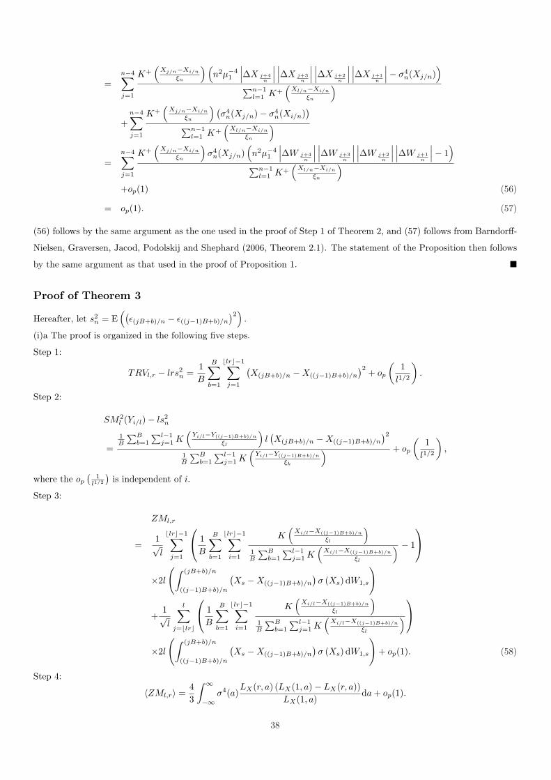
=n−4∑

j=1

K+(

Xj/n−Xi/n

ξn

) (n2µ−4

1

∣∣∣∆X j+4n

∣∣∣∣∣∣∆X j+3

n

∣∣∣∣∣∣∆X j+2

n

∣∣∣∣∣∣∆X j+1

n

∣∣∣− σ4n(Xj/n)

)

∑n−1l=1 K+

(Xl/n−Xi/n

ξn

)

+n−4∑

j=1

K+(

Xj/n−Xi/n

ξn

) (σ4

n(Xj/n)− σ4n(Xi/n)

)

∑n−1l=1 K+

(Xl/n−Xi/n

ξn

)

=n−4∑

j=1

K+(

Xj/n−Xi/n

ξn

)σ4

n(Xj/n)(n2µ−4

1

∣∣∣∆W j+4n

∣∣∣∣∣∣∆W j+3

n

∣∣∣∣∣∣∆W j+2

n

∣∣∣∣∣∣∆W j+1

n

∣∣∣− 1)

∑n−1l=1 K+

(Xl/n−Xi/n

ξn

)

+op(1) (56)

= op(1). (57)

(56) follows by the same argument as the one used in the proof of Step 1 of Theorem 2, and (57) follows from Barndorff-

Nielsen, Graversen, Jacod, Podolskij and Shephard (2006, Theorem 2.1). The statement of the Proposition then follows

by the same argument as that used in the proof of Proposition 1. ¥

Proof of Theorem 3

Hereafter, let s2n = E

((ε(jB+b)/n − ε((j−1)B+b)/n

)2)

.

(i)a The proof is organized in the following five steps.

Step 1:

TRVl,r − lrs2n =

1B

B∑

b=1

blrc−1∑

j=1

(X(jB+b)/n −X((j−1)B+b)/n

)2 + op

(1

l1/2

).

Step 2:

SM2l (Yi/l)− ls2

n

=1B

∑Bb=1

∑l−1j=1 K

(Yi/l−Y((j−1)B+b)/n

ξl

)l(X(jB+b)/n −X((j−1)B+b)/n

)2

1B

∑Bb=1

∑l−1j=1 K

(Yi/l−Y((j−1)B+b)/n

ξk

) + op

(1

l1/2

),

where the op

(1

l1/2

)is independent of i.

Step 3:

ZMl,r

=1√l

blrc−1∑

j=1

1

B

B∑

b=1

blrc−1∑

i=1

K(

Xi/l−X((j−1)B+b)/n

ξl

)

1B

∑Bb=1

∑l−1j=1 K

(Xi/l−X((j−1)B+b)/n

ξl

) − 1

×2l

(∫ (jB+b)/n

((j−1)B+b)/n

(Xs −X((j−1)B+b)/n

)σ (Xs) dW1,s

)

+1√l

l∑

j=blrc

1

B

B∑

b=1

blrc−1∑

i=1

K(

Xi/l−X((j−1)B+b)/n

ξl

)

1B

∑Bb=1

∑l−1j=1 K

(Xi/l−X((j−1)B+b)/n

ξl

)

×2l

(∫ (jB+b)/n

((j−1)B+b)/n

(Xs −X((j−1)B+b)/n

)σ (Xs) dW1,s

)+ op(1). (58)

Step 4:

〈ZMl,r〉 =43

∫ ∞

−∞σ4(a)

LX(r, a) (LX(1, a)− LX(r, a))LX(1, a)

da + op(1).

38

Step 5:

ZMl,rd−→ MN

(0,

43

∫ ∞

−∞

(LX(a, r) (LX(1, a)− LX(r, a)

L(1, a)

)σ4(a)da

).

(i)b and (ii) follow by the same argument as in the proof of Theorem 1.

Proof of Step 1:

√l

B

B∑

b=1

blrc−1∑

j=1

((Y(jB+b)/n − Y((j−1)B+b)/n

)2 − s2n

)

=

√l

B

B∑

b=1

blrc−1∑

j=1

(X(jB+b)/n −X((j−1)B+b)/n

)2

+ 2

√l

B

B∑

b=1

blrc−1∑

j=1

(ε(jB+b)/n − ε((j−1)B+b)/n

) (X(jB+b)/n −X((j−1)B+b)/n

)(59)

+

√l

B

B∑

b=1

blrc−1∑

j=1

((ε(jB+b)/n − ε((j−1)B+b)/n

)2 − s2n

). (60)

We begin by considering the term in (60). As εj/n = Op(an), s2n = O(a2

n), and Bl = n,

lvar

1

B

B∑

b=1

blrc−1∑

j=1

a2n

((ε(jB+b)/n − ε((j−1)B+b)/n

an

)2

− s2n

a2n

)

= lOp

(la4

nB−1)

= op(1),

given that anξ−1l → 0 and ξllB

−1/2 → 0 imply l2a2nB−1 → 0. Since E

(εj/nXj

)= 0, then the term in (59) is op(l−1/2),

regardless of the rate at which an → 0, by the same argument as in the proof of Theorem 1 in Zhang, Mykland and

Aıt-Sahalia (2005).

Proof of Step 2:

1√l

blrc−1∑

i=1

(SM2

l (Yi/l)− ls2n

)

=1√l

blrc−1∑

i=1

1B

∑Bb=1

∑l−1j=1 K

(Yi/l−Y((j−1)B+b)/n

ξl

)l((

Y(jB+b)/n − Y((j−1)B+b)/n

)2 − s2n

)

1B

∑Bb=1

∑l−1j=1 K

(Yi/l−Y((j−1)B+b)/n

ξl

)

=1√l

blrc−1∑

i=1

1B

∑Bb=1

∑l−1j=1 K

(Yi/l−Y((j−1)B+b)/n

ξl

)l(X(jB+b)/n −X((j−1)B+b)/n

)2

1B

∑Bb=1

∑l−1j=1 K

(Yi/l−Y((j−1)B+b)/n

ξl

)

+2√l

blrc−1∑

i=1

×

1B

∑Bb=1

∑l−1j=1 K

(Yi/l−Y((j−1)B+b)/n

ξl

)l(X(jB+b)/n −X((j−1)B+b)/n

) (ε(jB+b)/n − ε((j−1)B+b)/n

)

1B

∑Bb=1

∑l−1j=1 K

(Yi/l−Y((j−1)B+b)/n

ξl

) (61)

+1√l

blrc−1∑

i=1

1B

∑Bb=1

∑l−1j=1 K

(Yi/l−Y((j−1)B+b)/n

ξl

)l((

ε(jB+b)/n − ε((j−1)B+b)/n

)2 − s2n

)

1B

∑Bb=1

∑l−1j=1 K

(Yi/l−Y((j−1)B+b)/n

ξl

) . (62)

By the same argument as in Step 1, the term in (62) is of a larger probability order than the one in (61) (involving the

cross term between log-efficient price and microstructure noise). Thus, it suffices to show the term in (62) is op(1).

39

We can rewrite it as

1√l

blrc−1∑

i=1

1Bξ

∑Bb=1

∑l−1j=1 K

(Yi/l−Y((j−1)B+b)/n

ξl

)((ε(jB+b)/n − ε((j−1)B+b)/n

)2 − s2n

)

1Blξ

∑Bb=1

∑l−1j=1 K

(Yi/l−Y((j−1)B+b)/n

ξl

) .

As anξ−1 →∞,

1Blξ

B∑

b=1

l−1∑

j=1

K

(Yi/l − Y((j−1)B+b)/n

ξl

)

=1

Blξ

B∑

b=1

l−1∑

j=1

K

(Xi/l −X((j−1)B+b)/n

ξl

)

︸ ︷︷ ︸Op(1)

+ op(1), (63)

uniformly in i. The Op(1) term above is bounded away from zero, because it converges to the the local time of the

diffusion evaluated at Xi/l. Finally,

var

1√l

blrc−1∑

i=1

1Bξ

∑Bb=1

∑l−1j=1 K

(Yi/l−Y((j−1)B+b)/n

ξl

)a2

n

((ε(jB+b)/n−ε((j−1)B+b)/n

an

)2

− s2n

a2n

)

1Blξ

∑Bb=1

∑l−1j=1 K

(Yi/l−Y((j−1)B+b)/n

ξl

)

= a4nOp

(l2

Bξ2

)= op(1),

since ξ−1l an → 0 and this, togheter with the condition ξllB

−1/2 → 0, implies l2a2nB−1 → 0.

Proof of Step 3:

Given Step 1 and 2,

ZMl,r

=1√l

blrc−1∑

i=1

1B

∑Bb=1

∑l−1j=1 K

(Yi/l−Y((j−1)B+b)/n

ξl

)l

((X(jB+b)/n −X((j−1)B+b)/n

)2 − σ2(Xi/l)l

)

1B

∑Bb=1

∑l−1j=1 K

(Yi/l−Y((j−1)B+b)/n

ξl

)

−√

l

B

B∑

b=1

blrc−1∑

j=1

((X(jB+b)/n −X((j−1)B+b)/n

)2 − σ2(X((j−1)B+b)/n

))+ op(1). (64)

By Ito’s formula,

√l

B

B∑

b=1

blrc−1∑

j=1

((X(jB+b)/n −X((j−1)B+b)/n

)2 − σ2(X((j−1)B+b)/n

))

=2√

l

B

B∑

b=1

blrc−1∑

j=1

∫ (Xs −X((j−1)B+b)/n

)σ (Xs) dW1,s + op(1).

For any i, by a mean value expansion around εi/l − ε((j−1)B+b)/n = 0, we have

K

(Yi/l − Y((j−1)B+b)/n

ξl

)= K

(Xi/l −X((j−1)B+b)/n

ξl

)+ K ′

(Y i/l − Y ((j−1)B+b)/n

ξl

)εi/l − ε((j−1)B+b)/n

ξl,

where Y ((j−1)B+b)/n ∈(Y((j−1)B+b)/n, X((j−1)B+b)/n

). As K ′ is bounded and

εi/l−ε((j−1)B+b)/n = Op (an) = op (ξl) ,

40

uniformly in i, j, the first term of the tight hand side of (64) can be rewritten as

1√l

blrc−1∑

i=1

(SM2

l (Xi/l)− σ2(Xi/l))

=1√l

blrc−1∑

i=1

1B

∑Bb=1

∑l−1j=1 K

(Xi/l−X((j−1)B+b)/n

ξl

)l

(∫ (jB+b)/n

((j−1)B+b)/nσ2(Xs)ds− σ2(Xi/l)

l

)

1B

∑Bb=1

∑l−1j=1 K

(Xi/l−X((j−1)B+b)/n

ξl

)

(65)

+1√l

blrc−1∑

i=1

1B

∑Bb=1

∑l−1j=1 K

(Xi/l−X((j−1)B+b)/n

ξl

)2l

(∫ (jB+b)/n

((j−1)B+b)/n

(Xs −X((j−1)B+b)/n

)σ (Xs) dW1,s

)

1B

∑Bb=1

∑l−1j=1 K

(Xi/l−X((j−1)B+b)/n

ξl

)

=1√l

blrc−1∑

i=1

1B

∑Bb=1

∑l−1j=1 K

(Xi/l−X((j−1)B+b)/n

ξl

)2l

(∫ (jB+b)/n

((j−1)B+b)/n

(Xs −X((j−1)B+b)/n

)σ (Xs) dW1,s

)

1B

∑Bb=1

∑l−1j=1 K

(Xi/l−X((j−1)B+b)/n

ξl

)

+op(1), (66)

as (65) is op(1), given that l1/2+εξl → 0. The statement in Step 3 then follows by simple algebra, along the same lines as

in the proof of Theorem 1.

Proof of Step 4:

Let ZM(1)l,r and ZM

(2)l,r denote the first and second term of the right hand side of (58), respectively. Then, up to a op(1)

term,

⟨ZM

(1)l,r

⟩

=1

lB2

B∑

b=1

B∑

k=1

blrc−1∑

j=1blrc−1∑

i=1

blrc−1∑

i′=1

K(

Xi/l−X((j−1)B+b)/n

ξl

)K

(Xi′/l−X((j−1)B+k)/n

ξl

)

1B

∑nj=1 K

(Xi/l−X(j−1)/n

ξl

)1B

∑nj=1 K

(Xi′/l−X(j−1)/n

ξl

) + 1− 2blrc−1∑

i=1

K(

Xi/l−X((j−1)B+b)/n

ξl

)

1B

∑nj=1 K

(Xi/l−X(j−1)/n

ξl

)

×⟨

2l

∫ (jB+b)/n

((j−1)B+b)/n

(Xs −X((j−1)B+b)/n

)σ (Xs) dW1,s, 2l

∫ (jB+k)/n

((j−1)B+k)/n

(Xs −X((j−1)B+k)/n

)σ (Xs) dW1,s

⟩.

Now,∫ (jB+b)/n

((j−1)B+b)/n

(Xs −X((j−1)B+b)/n

)dW1,s is a martingale difference sequence; hence, for k > b,

⟨2l

∫ (jB+b)/n

((j−1)B+b)/n

(Xs −X((j−1)B+b)/n

)σ (Xs) dW1,s, 2l

∫ (jB+k)/n

((j−1)B+k)/n

(Xs −X((j−1)B+k)/n

)σ (Xs) dW1,s

⟩

=

⟨2l

∫ (jB+b)/n

((j−1)B+k)/n

(Xs −X((j−1)B+k)/n

)σ (Xs) dW1,s

⟩

= 2σ4(X((j−1)B+k)/n

)(1−

(k − b

B

))2

+ op(1).

Thus,

⟨ZM

(1)l,r

⟩

=4

lB2

B∑

b=1

blrc−1∑

j=1

41

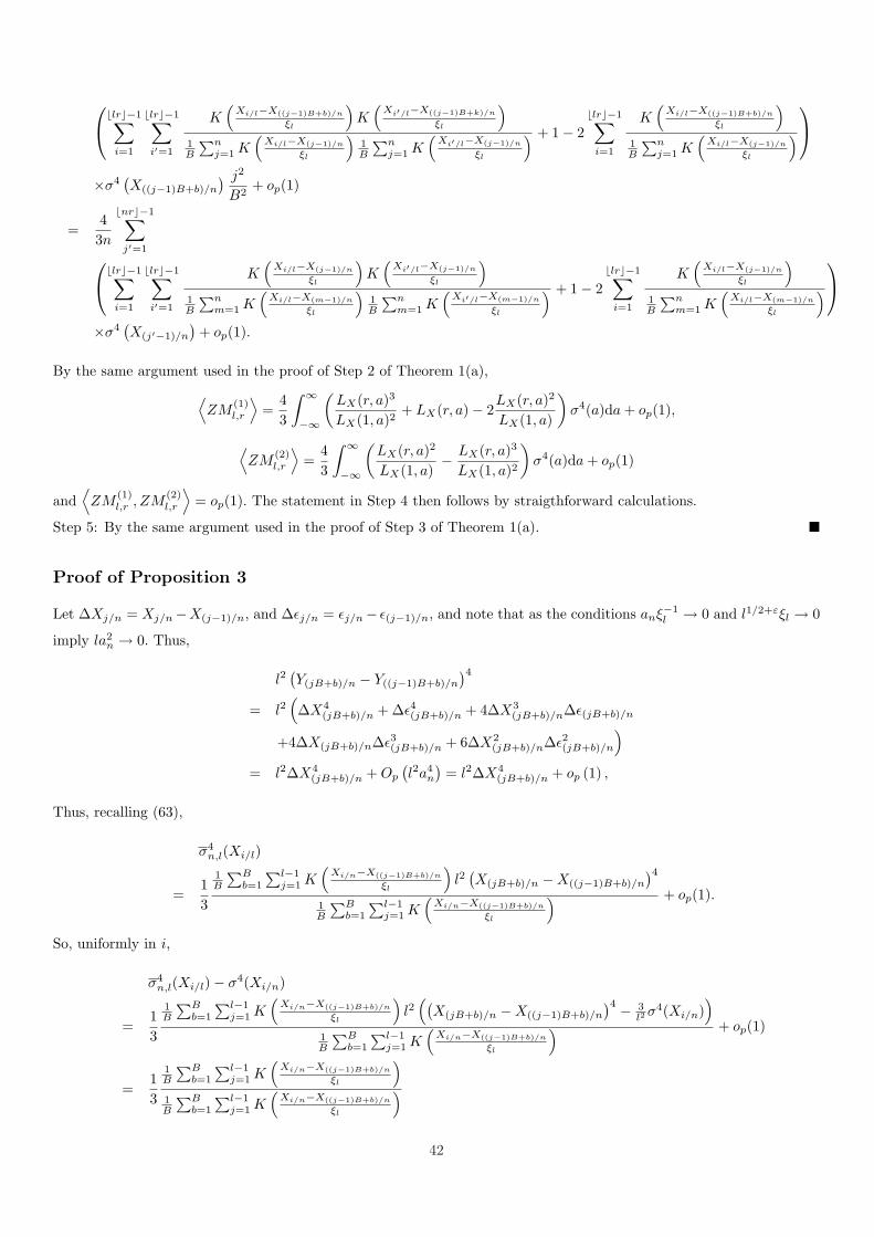
blrc−1∑

i=1

blrc−1∑

i′=1

K(

Xi/l−X((j−1)B+b)/n

ξl

)K

(Xi′/l−X((j−1)B+k)/n

ξl

)

1B

∑nj=1 K

(Xi/l−X(j−1)/n

ξl

)1B

∑nj=1 K

(Xi′/l−X(j−1)/n

ξl

) + 1− 2blrc−1∑

i=1

K(

Xi/l−X((j−1)B+b)/n

ξl

)

1B

∑nj=1 K

(Xi/l−X(j−1)/n

ξl

)

×σ4(X((j−1)B+b)/n

) j2

B2+ op(1)

=43n

bnrc−1∑

j′=1blrc−1∑

i=1

blrc−1∑

i′=1

K(

Xi/l−X(j−1)/n

ξl

)K

(Xi′/l−X(j−1)/n

ξl

)

1B

∑nm=1 K

(Xi/l−X(m−1)/n

ξl

)1B

∑nm=1 K

(Xi′/l−X(m−1)/n

ξl

) + 1− 2blrc−1∑

i=1

K(

Xi/l−X(j−1)/n

ξl

)

1B

∑nm=1 K

(Xi/l−X(m−1)/n

ξl

)

×σ4(X(j′−1)/n

)+ op(1).

By the same argument used in the proof of Step 2 of Theorem 1(a),

⟨ZM

(1)l,r

⟩=

43

∫ ∞

−∞

(LX(r, a)3

LX(1, a)2+ LX(r, a)− 2

LX(r, a)2

LX(1, a)

)σ4(a)da + op(1),

⟨ZM

(2)l,r

⟩=

43

∫ ∞

−∞

(LX(r, a)2

LX(1, a)− LX(r, a)3

LX(1, a)2

)σ4(a)da + op(1)

and⟨ZM

(1)l,r , ZM

(2)l,r

⟩= op(1). The statement in Step 4 then follows by straigthforward calculations.

Step 5: By the same argument used in the proof of Step 3 of Theorem 1(a). ¥

Proof of Proposition 3

Let ∆Xj/n = Xj/n−X(j−1)/n, and ∆εj/n = εj/n− ε(j−1)/n, and note that as the conditions anξ−1l → 0 and l1/2+εξl → 0

imply la2n → 0. Thus,

l2(Y(jB+b)/n − Y((j−1)B+b)/n

)4

= l2(∆X4

(jB+b)/n + ∆ε4(jB+b)/n + 4∆X3(jB+b)/n∆ε(jB+b)/n

+4∆X(jB+b)/n∆ε3(jB+b)/n + 6∆X2(jB+b)/n∆ε2(jB+b)/n

)

= l2∆X4(jB+b)/n + Op

(l2a4

n

)= l2∆X4

(jB+b)/n + op (1) ,

Thus, recalling (63),

σ4n,l(Xi/l)

=13

1B

∑Bb=1

∑l−1j=1 K

(Xi/n−X((j−1)B+b)/n

ξl

)l2

(X(jB+b)/n −X((j−1)B+b)/n

)4

1B

∑Bb=1

∑l−1j=1 K

(Xi/n−X((j−1)B+b)/n

ξl

) + op(1).

So, uniformly in i,

σ4n,l(Xi/l)− σ4(Xi/n)

=13

1B

∑Bb=1

∑l−1j=1 K

(Xi/n−X((j−1)B+b)/n

ξl

)l2

((X(jB+b)/n −X((j−1)B+b)/n

)4 − 3l2 σ4(Xi/n)

)

1B

∑Bb=1

∑l−1j=1 K

(Xi/n−X((j−1)B+b)/n

ξl

) + op(1)

=13

1B

∑Bb=1

∑l−1j=1 K

(Xi/n−X((j−1)B+b)/n

ξl

)

1B

∑Bb=1

∑l−1j=1 K

(Xi/n−X((j−1)B+b)/n

ξl

)

42

×l2

σ4(X((j−1)B+b)/n)

(∫ (jB+b)/n

((j−1)B+b)/n

dW1,s

)4

− 3l2

σ4(X((j−1)B+b)/n)

+ op(1)

=13

1lBξl

∑Bb=1

∑l−1j=1 K

(Xi/n−X((j−1)B+b)/n

ξl

)σ4(X((j−1)B+b)/n)

(u4

((j−1)B+b)/n− 3

)

1lξlB

∑Bb=1

∑l−1j=1 K

(Xi/n−X((j−1)B+b)/n

ξl

) + op(1)

=13

1nξl

∑nj=1 K

(Xi/n−X(j−1)/n

ξl

)σ4(X(j−1)/n)

(u4

j− 3

)

1nζl

∑nj=1 K

(Xi/n−X(j−1)/n

ξl

) + op(1) (67)

and uj are N(0, 1), and E((

u4j− 3

) (u4

k− 3

))= 0 for |j − k| > B.

Thus,

1nξln

n∑

j=1

K

(Xi/n −X(j−1)/n

ξl

)σ4(X(j−1)/n)

(u4

j− 3

)

= Op

(√nBξl

n2ξ2l

)= Op

(√1lξl

)= op(1),

as lξl →∞. The rest of the proof then follows along the same lines in the proof of Proposition 1. ¥

43

References

Aıt-Sahalia, Y. (1996a). Nonparametric Pricing of Interest Rate Derivative Securities. Econometrica, 64, 527-561.

Aıt-Sahalia, Y. (1996b). Testing Continuous-Time Models of the Spot Interest Rate. Review of Financial Studies, 9,

385-426.

Aıt-Sahalia, Y., P.A. Mykland and L. Zhang (2006). Ultra High Frequency Volatility Estimation and Dependent

Microstructure Noise. Manuscript, Princeton University.

Andersen, T.G., L. Benzoni and J. Lund (2002). An Empirical Investigation of Continuous Time Equity Returns

Models. Journal of Finance, VLII, 1239-1284.

Andersen, T.G., T. Bollerslev, F.X. Diebold and P. Labys (2001). The Distribution of Realized Exchange Rate Volatility.

Journal of the American Statistical Association, 96, 42-55.

Ang, A. and M. Piazzesi (2003). A No-Arbitrage Vector Autoregression of Term Structure Dynamics with Macroeco-

nomic and Latent Variables. Journal of Monetary Economics, 50, 745-787.

Awartani, B., V. Corradi and W. Distaso (2006). Testing Market Microstructure Effects with an Application to the

Dow Jones Industrial Average Stocks. Working Paper, Tanaka Business School, Imperial College, London.

Bakshi, G., C. Cao and Z.W. Chen (2000). Do Call Prices and the Underlying Stock Always Move in the Same Direction?

Review of Financial Studies, 13, 549-584.

Bandi, F.M. and T.H. Nguyen (2003). On the Functional Estimation of Jump Diffusion Models. Journal of Economet-

rics, 116, 293-328.

Bandi, F.M. and P.C.B. Phillips (2003). Fully Nonparametric Estimation of Scalar Diffusion Models. Econometrica,

71, 241-283.

Bandi, F.M. and P.C.B. Phillips (2007). A Simple Approach to the Parametric Estimation of Potentially Nonstationary

Diffusions. Journal of Econometrics, 137, 354-395.

Bandi, F.M. and J.R. Russell (2007). Market Microstructure Noise, Integrated Variance Estimators, and the Accuracy

of Asymptotic Approximations. Working Paper, University of Chicago, Graduate School of Business.

Barndorff-Nielsen, O.E., S.E. Graversen, J. Jacod, M. Podolskij and N. Shephard (2006). A central limit theorem for

realised power and bipower variations of continuous semimartingales. In Kabanov, Y., R. Lipster and J. Stoyanov

(eds.), From Stochastic Analysis to Mathematical Finance, Festschrift for Albert Shiryaev, pp. 33-68, Springer,

New York.

Barndorff-Nielsen, O.E., P.R. Hansen, A. Lunde and N. Shephard (2006). Designing Realised Kernels to Measure the

Ex-Post Variation of Equity Prices in the Presence of Noise. Manuscript, University of Oxford.

44

Barndorff-Nielsen, O.E., P.R. Hansen, A. Lunde and N. Shephard (2007). Subsampling Realised Kernels. Working

Paper, Oxford University.

Barndorff-Nielsen, O.E. and N. Shephard (2002). Econometric Analysis of Realized Volatility and Its Use in Estimating

Stochastic Volatility Models. Journal of the Royal Statistical Society, Series B, 64, 253-280.

Barndorff-Nielsen, O.E. and N. Shephard (2004). Power and Bipower Variation with Stochastic Volatility and Jumps

(with Discussion). Journal of Financial Econometrics, 2, 1-48.

Barndorff-Nielsen, O.E., N. Shephard and M. Winkel (2006). Limit Theorems for Multipower Variation in the Presence

of Jumps. Stochastic Processes and Their Applications, 116, 796-806.

Bergman, Y.Z., B.D. Grundy and Z. Wiener (1996). General Properties of Option Prices. Journal of Finance, LI,

1573-1610.

Bibkov, R. and M. Chernov (2006). No-Arbitrage Macroeconomic Determinants of the Yield Curve. Working Paper,

London Business School.

Black, F., E. Derman and W. Toy (1990). A One-Factor Model of Interest Rates and its Application to treasury Bond

Options. Financial Analyst Journal, 46, 33-39.

Buraschi, A. and F. Corielli (2005). Risk management implications of time-inconsistency: model updating and recali-

bration of no-arbitrage models. Journal of Banking and Finance, 29, 2883-2907.

Buraschi, A. and J. Jackwerth (2001). The Price of a Smile: Hedging and Spanning in Option Markets. Review of

Financial Studies, 14, 495-527.

Buraschi, A. and A. Jiltsov (2006). Model Uncertainty and Option Markets with Heterogeneous Beliefs. Journal of

Finance, LXI, 2841-2897.

Chapman, D.A. and N.D. Pearson (2000). Is the Short Rate Drift Actually Nonlinear? Journal of Finance, LV, 355-388.

Cont, R. and P. Tankov (2004). Financial Modelling With Jump Processes. Chapman and Hall, New York.

Corradi, V., W. Distaso and A. Mele (2006). Macroeconomics Strikes Back: Real Determinants of Volatility Risk-

Premia. Working Paper, Tanaka Business School, Imperial College, London.

Cox, J.C., J.E. Ingersoll and S.A. Ross (1985). A Theory of the Term Structure of Interest Rates. Econometrica, 53,

385-407.

Derman, E. and I. Kani (1994). Riding on a smile. Risk, 7 , 32-39.

Dumas, B., J. Fleming, and R.E. Whaley (1998). Implied volatility functions: Empirical tests. Journal of Finance,

LIII, 2059-2106.

45

Dupire, B. (1994). Pricing with a smile. Risk, 7, 18-20.

Fan, J. (2005). A Selective Overview of Nonparametric Methods in Financial Econometrics (with discussion). Statistical

Science, 20, 317-357.

Fan, J. and Y.K. Truong (1993). Nonparametric Regression with Errors in Variables. Annals of Statistics, 21, 1900-1925.

Florens-Zmirou, D. (1993). On Estimating the Diffusion Coefficient from Discrete Observations. Journal of Applied

Probability, 30, 790-804.

Fong, H.G. and O.A. Vasicek (1992). Interest Rate Volatility as a Stochastic Factor. Gifford Fong Associates Working

Paper.

Heath, D., R.A. Jarrow and A.J. Morton (2002). Bond Pricing and the Term Structure of Interest Rates: A New

Methodology for Contingent Claims Valuation. Econometrica, 60, 77-105.

Heston, S. (1993). A closed-form solution for options with stochastic volatility with applications to bond and currency

options. Review of Financial Studies, 6, 327-343.

Hong, Y. and H. Li (2005). Nonparametric Specification Testing for Continuous-Time Models with Applications to

Term Structure of Interest Rates. Review of Financial Studies, 18, 37-84.

Hull, J.C. and A.D. White (1987). The Pricing of Options on Assets with Stochastic Volatilities. Journal of Finance,

XLII, 281-300.

Jacod, J. (1994). Limit of Random Measures Associated with the Increments of a Brownian Semimartingale. Preprint

number 120, Laboratoire de Probabilities, Universite Pierre et Marie Curie, Paris.

Jacod, J. and P. Protter (1998). Asymptotic Error Distribution for the Euler Method for Stochastic Differential

Equations. Annals of Probability, 26, 267-307.

James, J. and N. Webber (2000). Interest Rate Modelling. Wiley, Chichester.

Kalnina, I. and O. Linton (2007). Inference About Realized Volatility Using Infill Subsampling. Working Paper, LSE.

Karatzsas, I. and S.E. Shreve (1991). Brownian Motion and Stochastic Calculus. Springer Verlag, New York.

Mancini, C. and R. Reno (2006). Threshold Estimation of Jump-Diffusion Models and Interest Rate Modelling.

Manuscript, University of Siena.

Pardoux, E. and D. Talay (1985).Discretization and Simulation of Stochastic Differential Equations. Acta Applicandae

Mathematicae, 3, 23-47.

Piazzesi, M. (2005). Bond Yields and the Federal Reserve. Journal of Political Economy, 113, 311-344.

46

Pritsker, M. (1998). Nonparametric Density Estimation of Tests of Continuous Time Interest Rate Models. Review of

Financial Studies, 11, 449-487.

Schennach, S.M. (2004). Nonparametric Regression in the Presence of Measurement Error. Econometric Theory, 20,

1046–1093.

Stanton, R. (1997). A Nonparametric Model of Term Structure Dynamics and the Market Price of Interest Rate Risk.

Journal of Finance, LII, 1973-2002.

Stein, E. and J.C. Stein (1991). Stock Price Distributions with Stochastic Volatility: An Analytic Approach. Review

of Financial Studies, 4, 727-752.

Vasicek, O.A. (1977). An Equilibrium Characterization of the Term Structure. Journal of Financial Economics, 5,

177-188.

Zhang, L. (2006). Efficient Estimation of Stochastic Volatility Using Noisy Observations: A Multi-Scale Approach.

Bernoulli, 12, 1019-1043.

Zhang, L., P.A. Mykland and Y. Aıt-Sahalia (2005). A Tale of Two Time Scales: Determining Integrated Volatility

with Noisy High Frequency Data. Journal of the American Statistical Association, 100, 1394-1411.

Zhang, L., P.A. Mykland and Y. Aıt-Sahalia (2006). Edgeworth Expansions for Realized Volatility and Related Esti-

mators, Manuscript, Princeton University.

47