Determining the Pattern Regeneration for a Cleared ...

MARCH

2001

Restoration Ecology Vol. 9 No. 1, pp. 1–12

1

©

2001 Society for Ecological Restoration

Determining the Pattern of Oak Woodland Regeneration for a Cleared Watershed in Northwest California:A Necessary First Step for Restoration

Colin N. Brooks

1,3

Adina M. Merenlender

2

Abstract

Historically, oak woodlands of northern Californiahave been subject to intensive tree and brush removalefforts to improve land for livestock grazing. As a re-sult of this tree removal, these watersheds are suscep-tible to soil erosion and stream degradation. There-fore, planting woody vegetation is often required torestore watershed function. Prior to such actions, athorough understanding of natural vegetation regen-eration patterns is essential. The physical and biologi-cal attributes of natural vegetation regeneration in acleared watershed were characterized using remotesensing, a Geographic Information System, and fieldsurveys. A 79-ha watershed at the University of Cali-fornia’s Hopland Research and Extension Center wasexamined because the clearing of vegetation was partof a well-documented experiment in the early 1960s,providing essential baseline data. The results of thisstudy reveal that significantly more oak regeneration,consisting mostly of evergreen oaks, occurred onmoister and steeper northerly slopes. Deciduous oaks,

located primarily on drier and less steep southerlyslopes, have not regenerated. Hardwood regenerationwas associated with Josephine, Los Gatos, and May-men soils. The distribution of hardwood regenerationis clustered, suggesting that the presence of othertrees may promote regeneration. These results alsosuggest that without active restoration efforts such as

tree planting and seedling protection, southerly slopeswill most likely remain barren and erosion will con-tinue, while northerly slopes and riparian areas willrecover under the current land management practices.Despite some woody plant regeneration, the oncedensely forested watershed is now predominantlygrassland, emphasizing the need to minimize clearingof California oak woodlands.

Key words:

GIS, hardwoods, spatial analysis, range-

land,

Quercus

.

Introduction

S

ince the first European settlement of the mid-1700s,activities such as logging, grazing, mining, build-

ing, and farming have altered California’s plant com-munities and affected the state’s biodiversity (Barbouret al. 1993). In particular, the clearing of woodland andbrushland for the benefit of livestock was a commonpractice in the decades following World War II. Im-proving forage production, increasing water yield, pro-viding better wildlife habitat, controlling fire risk, andimproving visual aesthetics were some of the reasonsgiven for removing overstory vegetation (Johnson et al.1959; Murphy & Berry 1973; Heady & Pitt 1979). Suchclearing left a legacy of open hillsides with changed wa-ter regimes covered by exotic annual grasslands (Hol-land 1980; Murphy 1980) and contributed to a loss ofone million acres of California’s oak woodlands be-tween 1945 and 1973 (Bolsinger 1988).

To compound the problem, several species of Califor-nia oaks currently have low rates of natural regenera-tion in portions of the state (Bolsinger 1988). Concernfor oak woodland conservation in California has led toactive restoration efforts. Much of the research on oakregeneration is focused on planting experiments de-signed to determine the limiting factors to seedling de-velopment (Muick 1991; Tietje et al. 1991; Adams et al.1997; McCreary & Lippitt 1997). Several projects haveinvolved planting thousands of oaks across multipleacres (Nives et al. 1991; Griggs et al. 1997), demonstrat-ing the need for an understanding of the influence oflandscape variability and ecosystem processes on oakestablishment. At the landscape scale, oak woodlandmonitoring and research have been limited to docu-menting habitat loss through various methods of habi-

1

Hopland Research and Extension Center, 4070 University Road, Hopland, CA 95449, U.S.A.

2

Environmental Science, Policy and Management, University of California, Berkeley, CA 94720–3110, U.S.A.

3

Address correspondence to C. Brooks, email cbrooks@ nature.berkeley.edu

Dertermining Oak Woodland Regeneration Patterns

2

Restoration Ecology

MARCH

2001

tat change detection (McKay 1987) and have not, todate, focused on spatial patterns of natural regenera-tion. With the exception of recent research done in Is-rael by Carmel and Kadmon (1998), this appears tohave rarely been considered when investigating hard-wood regeneration. A better understanding of the natu-ral restoration process and pattern is essential to deter-mine the most appropriate location, distribution, andspecies composition that should be established for oakwoodland restoration.

This study characterized the spatial pattern, physio-graphic correlates, and species composition of naturalvegetation that has regenerated in a watershed that wascleared between 1959 and 1965. This watershed waswell studied as part of a rangeland productivity and wa-ter yield study, providing us with critical information onthe original vegetation coverage, methods of vegetationremoval, and immediate results of the clearing.

Physiographic parameters including the slope, as-pect, and soil types and biological parameters includingchanges in overall cover type, the distribution patternsof trees in the watersheds, and the species compositionin areas of regeneration were examined. A geographicinformation system (GIS) was used to quantify vegeta-tion change soon after and since the watershed wascleared of most of its woody vegetation, and to analyzespatial patterns of vegetation. This relatively new ap-proach may provide the basis for an innovative methodthat could be used by others to study the principles ofplant community replacement at a wide range of spatialscales.

Study Area

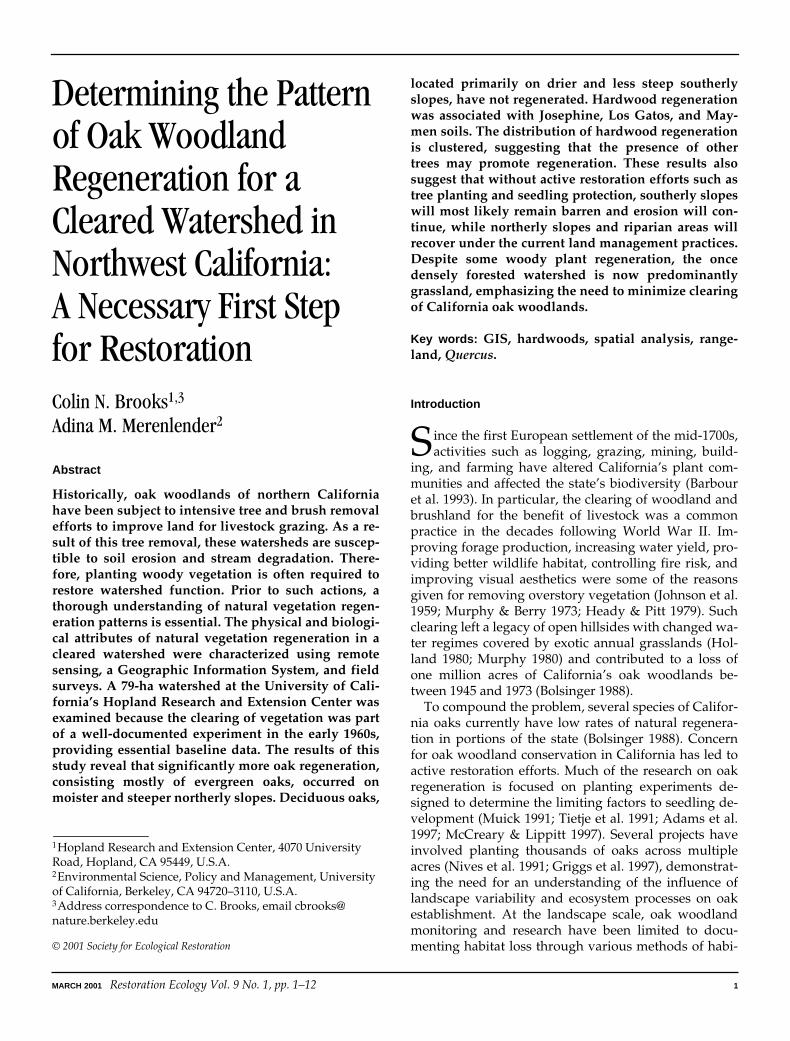
The study watershed is located on the University ofCalifornia’s Hopland Research and Extension Center(HREC), located in Mendocino County in the north-cen-tral portion of the California coastal mountain ranges(Fig. 1). This watershed site has a drainage basin of 78.8ha, ranges in elevation from 180 m to 403 m, and has aslope range of 2 to 40 degrees with a mean of 18 de-grees. It is in a typical Mediterranean climate zone ofhot, dry summers and cool, wet winters, and lies 65 kminland from the Pacific Ocean. Average annual rainfallis approximately 900 mm (Heady & Pitt 1979). The wa-tershed is located primarily on soils that have devel-oped from hard sandstone and shale (Josephine, Suth-erlin, and Laughlin series) (Gowans 1958). These soilsare part of the Franciscan formation and are approxi-mately one meter thick. Approximately 60 percent ofthe watershed is in south, southwest, or southeast-fac-ing slopes, and just under a quarter of the watershed isin north, northwest, or northeast-facing slopes. This wa-tershed is typical of rangeland areas in northwest Cali-fornia in terms of its long history of livestock grazing

and its annual grassland cover. According to a field sur-vey done in the 1950s, the pre-clearing vegetation wascomposed of 5 ha of grassland, 9 ha of chaparral, 20 haof mixed grassland and deciduous oaks, and approxi-mately 51 ha of hardwood forest primarily consisting of

Quercus wislizeni

(interior live oak),

Q. agrifolia

(coastlive oak),

Q. douglasii

(blue oak),

Q. kelloggii

(black oak),and

Arbutus menziesii

(madrone) (Murphy 1976).Vegetation removal for a rangeland productivity and

water yield study started in December 1959 and wascompleted in July 1965. The objective was to removemost of the woody vegetation; however, researchers de-cided to leave a few trees in the watershed for aestheticreasons and to provide shade for the sheep (CharlesVaughn & Milt Jones 1997, University of California -Davis, personal communication). An initial seeding ofgrasses and legumes was done via aircraft over the en-tire watershed one month before the start of vegetationremoval. This seeding consisted of a cultivar of

Trifo-lium subterraneum

(subclover), a cultivar of

Vicia villosassp. varia

(vetch),

T. incarnatum

(crimson clover), and

Phalaris aquatica

(harding grass). Trees were killed byapplying 2,4-D amine in surface cuts circling the base oftree trunks over a period of four months in late 1959and early 1960. Approximately half of the trees hadfallen by the end of 1964. Final clearing of woody vege-tation was completed in July 1965 with a prescribed firethat produced an intense burn with a convection col-umn of smoke that was over 1 km in height (Heady &Pitt 1979). In September 1965, additional grasses and le-

Figure 1. Locations of study watershed and Hopland Re-search & Extension Center (HREC).

Determining Oak Woodland Regeneration Patterns

MARCH

2001

Restoration Ecology

3

gumes were seeded over the entire watershed. This seed-ing included

Bromus hordeaceus

(soft chess), a cultivar of

Dactylis glomerata

(orchard grass),

Piptatherum miliaceum

(smilo grass), and additional T

. subterraneum

,

V. villosassp. varia

, and

P. aquatica

. Brush regeneration in someformer chaparral areas was controlled via summer andearly fall grazing, and by applying 2,4-D amine in 1967,1968, and 1969. However, the areas where this addi-tional brush control occurred were not recorded. Tan-dex (Ciba-Geigy, Greensboro, NC), a soil sterilizer, wasapplied to a small (approximately 1/5 ha) area of south-facing slope in February 1970; this area was reseededwith grasses in 1971, 1972, and 1973. These seedings in-cluded

B. hordeaceus

, four cultivars of

T. subterraneum,Trifolium hirtum

(rose clover), a cultivar of

T. hirtum

, acultivar of

D. glomerata

,

P. miliaceum

, and

P. aquatica

.Tens of thousands of tons of soil were lost through

erosion following the clearing, particularly after theroot systems of removed woody plants in the areas offormer riparian vegetation had decayed (Pitt et al.1978). From 1960 to 1970, 61 soil slips were documentedin the watershed (Burgy & Papazafiriou 1974). All theslips occurred in the vicinity of stream channels and inareas with a slope of greater than 24 degrees, and mosthappened in years of heavy rain. The only attempt tostabilize the soils was made in one small drainage byplanting

Salix lasiolepis

(arroyo willow) cuttings and

Cortaderia selloana

(pampas grass) in 1971 and 1974. The

S. lasiolepis

area covered about 1/4-ha while the

C. sel-loana

was planted in a few small clumps. Soil slips arestill occurring in this watershed, especially during peri-ods of heavy rainfall. While year-round water flow oc-curred in the years immediately following the experi-ment, surface flow today is intermittent during lowrainfall years.

Methods

Aerial Photo Time Series

In order to characterize vegetation regeneration, it wasnecessary to map the area at three points in time: beforeclearing, soon after clearing and burning, and a periodrepresenting the present day. Aerial photos that in-cluded a clear picture of the watershed for each of thethree time periods were obtained and scanned at 400 dpifor digital analysis. Photo dates and sources included:July 1952 (before), Agricultural Stabilization and Con-servation Service; October 1968 (after), USGS EROS DataCenter; and March 1996 (present day), WAC Corpora-tion (Fig. 2). While it would have been desirable to ob-tain photographs from the same season for each date,availability of clear historical photographs of similarand appropriate scales was limited to relatively fewyears and generally for only one or two days a year. As

tree and shrub outlines were clearly visible both inspring (March 1996) and fall (October 1968) photographs,seasonal differences did not prove to be a problem. Thesephotos were georeferenced so they could be integratedinto a GIS by comparing known ground-control points(GCPs) with identified sites on the watershed portion ofthe 1996 photo. Georeferencing was accomplished usingthe GCPWorks software package from PCI (RichmondHill, Canada). The GCPs were chosen because they wereclearly identifiable, evenly distributed on the 1996 aerialphotograph, and easily located in the field (e.g., road in-tersections, fence corners). The 1952 and 1968 photoswere georeferenced by registering them to the processed1996 photo. These three georeferenced images were thenimported into Arc/Info and ArcView (ESRI, Redlands,CA) for analysis and mapping.

Regeneration Classification

Vegetation cover maps were made for each georefer-enced photograph representing before clearing, afterthe 1965 burn, and present day periods. For each geo-referenced photo, areas of vegetation were digitized on-screen as polygons using ArcEdit, an Arc/Info program,while the photo was displayed in the background. Bydisplaying the photo at a large scale, fairly detailed map-ping of vegetation was possible. Emphasis was laid onmapping areas of tree and shrub vegetation so theycould later be identified as areas of regeneration or orig-inal vegetation. These mapped areas of woody plantscould range from a single tree or shrub in areas of scat-tered vegetation to multi-hectare groupings of trees andshrubs. Verification of vegetation type was done in thefield. With one exception, the following vegetation covertypes were identified and labeled for all three georefer-enced photos: 1) grass; 2) chaparral; 3) open hardwood;4) dense hardwood; 5) bare ground, roads, and build-ings; and 6) brush, shrubs, and young trees. The excep-tion, type 6, was not observed on the mature forest coverof the 1952 photograph. The last class was included fortwo reasons: some areas of existing shrub are not chap-arral, and it was occasionally difficult to differentiate be-tween small trees and shrubs, therefore they were in-cluded in a single class. Areas were labeled as “openhardwood” if they were clusters of hardwood trees in-terspersed with visible areas of grassland, while “densehardwood” had little or no grassland visible on theaerial photographs.

To characterize the patterns of vegetation change, itwas necessary to designate which vegetation polygonson the 1996 vegetation map were areas of woody plantregeneration (including both seedlings and sprouts), andwhich polygons represented areas of vegetation that hadsimply survived the clearing efforts of 1959 to 1965. Byoverlaying the digitized 1996 vegetation map over the


4

Restoration Ecology

MARCH

2001


MARCH

2001

Restoration Ecology

5

georeferenced 1968 photo, it was possible in almost allcases to distinguish which vegetation polygons were ar-eas of regeneration and to identify vegetation types. Somepolygons labeled as areas of tree or shrub regenerationdid include a few plants that had survived the clearing ef-forts, but these were generally a minor component. Thehardwood areas that survived the clearing efforts wereincluded in analysis results so that the physical and bio-logical attributes of these areas could also be character-ized. These were labeled as “survivor hardwood” sites.Altogether, the following types of regeneration were ana-lyzed: 1) upland hardwood regeneration; 2) riparianhardwood regeneration; 3) chaparral regeneration; and 4)survivor hardwood. A version of the 1996 vegetation mapwas created using these labels so that areas of regenera-tion could be clearly displayed (Fig. 3, 1996 vegetation).

Physiography and Soils

Physiographic parameters affecting regeneration (suchas slope, aspect, and soil type) were analyzed. The amountof each of the three regeneration types plus survivor hard-wood in each of eight slope classes was calculated in Arc-View by intersecting the 1996 regeneration map withslope grids derived from USGS digital elevation mod-els. The eight classes were defined by 5-degree incre-ments within the 0–40 degree range. The overall distri-bution of slopes for each of the regeneration types in thepresent day (1996) relative to their pre-clearing (1952)distributions was tested for a significant difference us-ing the non-parametric Kolmogorov-Smirnov test (Sokal& Rohlf 1995).

The individual slope, aspect, and soil classes of theregeneration types were compared to their distributionsin 1952 to see if some areas were more prone to regener-ation than others. Using these comparisons, it was pos-sible to determine if regeneration was over- or under-represented in a particular slope, aspect, and soil classrelative to the pre-clearing distribution for each vegeta-tion type. To test the statistical strength of this over- orunder-representation, individual confidence intervals werebuilt for each vegetation type using the square meter totalsof the types in 1996 as the observed values and the 1952area totals as the expected values. The Bonferroni correc-tion (Sokal & Rohlf 1995) was applied to each confi-dence interval so that the probability error rate could bebounded at

p

5

0.05 when estimating the categories ofthe physiographic variables simultaneously. This analy-sis is based on the work of Neu et al. (1974) and hasbeen used frequently when researchers are interested inover- or under-representation of a particular vegetationor habitat type by a study subject (Agee et al. 1989;

Stoms et al. 1992; McClean et al. 1998). The Kolmog-orov-Smirnov test was also applied to the 1952 and 1996aspect distributions. Aspect was analyzed similarly basedon the following eight categories: north (337.5

8

–22.5

8

),northeast (22.5

8

–67.5

8

), east (67.5

8

–112.5

8

), southeast (112.5

8

–157.5

8

), south (157.5

8

–202.5

8

), southwest (202.5

8

–247.5

8

),west (247.5

8

–292.5

8

), and northwest (292.5

8

–337.5

8

).Soils data were digitized from a published survey

done for the Hopland Research and Extension Center in1955 (Gowans 1958). This was a well-developed and de-tailed soil survey done at a relatively large scale usingthe nomenclature of the time. The names of the soiltypes used in this survey were not reassigned to reflectchanges in nomenclature implemented since 1955. Likethe slope and aspect analyses, the regeneration typeswere tested for a relationship with the soil type using theBonferroni-corrected confidence intervals method. Be-cause the Gowans survey did not map a separate soiltype for the narrow riparian zone, the riparian hardwoodregeneration class was not analyzed for this section.

Vegetation Distribution and Composition

Biological parameters related to the changes in vegeta-tion were also analyzed. The percent and absolute changesin amount of cover type were calculated from the 1952,1968, and 1996 vegetation maps using ArcView. The dis-tribution of trees in the watershed was analyzed to see ifit was clumped, random, or evenly distributed usingnearest neighbor analysis (Krebs 1989). The pattern of treedistribution was quantified using an index of aggrega-tion,

R

, and the standard normal deviate. These statisticswere calculated using an Avenue program adapted froman ArcView application. The Avenue program was mod-ified from its original form by allowing for a non-squarestudy boundary, and by taking into account trees imme-diately adjacent to the study watershed for nearest neigh-bor calculations. The data layer used for this analysis con-sisted of a point location for each individual tree in thewatershed observed on the 1996 photograph. Points fortrees outside the watershed boundary were also includedto allow for the buffer strip required for the unbiasedClark and Evans test (1954). This modified Avenue pro-gram can be obtained by contacting the authors. Thestand composition in regeneration and survivor areaswas determined in the field.

Results

The differences in pre-clearing, post-clearing, and presentday vegetation cover can be seen in the time series ofphotographs in Figure 2. Figure 3 shows the vegetation

Figure 2. Aerial photographs of study watershed before clearing, post clearing and burning, and the present day.


6

Restoration Ecology

MARCH

2001


MARCH

2001

Restoration Ecology

7

polygons digitized from the three time periods. This mapalso shows that areas of new upland and riparian hard-wood and chaparral vegetation appear to be clusteredin certain parts of the watershed (see the areas with abold outline in the 1996 vegetation panel of Fig. 3). A to-tal of 0.92 hectares of hardwood regeneration, 0.95 hect-ares of riparian hardwood regeneration, 1.24 hectares ofchaparral regeneration, and 2.28 hectares of survivorhardwood were identified on the 1996 vegetation map.


The distribution of the vegetation classes for 1952 and1996 in each slope, aspect, and soil category is pre-

sented in Tables 1a, 1b, and 1c, respectively. The Kol-mogorov-Smirnov tests reveal that present-day (1996)distributions are significantly different from the pre-clearing (1952) slope distribution for upland hardwood(

p

<

0.001, |

D

|

5

0.405) and chaparral regeneration (

p

<

0.001, |

D

|

5

0.481), but not for riparian hardwood re-generation (

p

.

0.10, |

D

|

5

0.121). Relative to the up-land hardwood distribution of 1952, areas of uplandhardwood regeneration are under-represented for 5–25degree slopes, and over-represented on 0–5 and 25–40degree slopes. The greatest over-representation is for25–35 degree slopes where 49.6% of upland hardwoodregeneration was located in 1996, and only 17.3% ofthese steep slopes were in hardwood in 1952. Riparian

Figure 3. Vegetation maps for the before clearing, post-clearing and burning, and present day photographs.

Table 1.

Comparison of 1996 distribution of regenerated chaparral, upland hardwood, and riparian hardwood to their distribution in 1952 for slope, aspect, and soil type.

1a. Slope Analysis 0–5 degrees 5–10 10–15 15–20 20–25 25–30 30–35 35–40

A. Upland hardwood regenerationProportion of area in 1952 0.013 0.048 0.168 0.315 0.284 0.142 0.026 0.005Proportion of area in 1996 0.020* 0.008* 0.090* 0.118* 0.268* 0.357* 0.128* 0.011*

B. Riparian hardwood regenerationProportion of area in 1952 0.071 0.129 0.376 0.230 0.135 0.028 0.019 0.013Proportion of area in 1996 0.051* 0.192* 0.376 0.291* 0.062* 0.012* 0.016 0.000*

C. Chaparral regenerationProportion of area in 1952 0.009 0.030 0.063 0.214 0.301 0.189 0.162 0.033Proportion of area in 1996 0.000* 0.000* 0.009* 0.153* 0.090* 0.064* 0.601* 0.084*

D. Survivor hardwoodProportion of area in 1996 0.032 0.041 0.404 0.302 0.165 0.050 0.005 0.000

1b. Aspect Analysis North Northeast East Southeast South Southwest West Northwest


B. Riparian hardwood regenerationProportion of area in 1952 0.026 0.000 0.000 0.062 0.307 0.236 0.185 0.184Proportion of area in 1996 0.000* 0.000 0.000 0.007* 0.230* 0.407* 0.171* 0.186

C. Chaparral regenerationProportion of area in 1952 0.000 0.001 0.000 0.118 0.473 0.323 0.070 0.015Proportion of area in 1996 0.000 0.000* 0.000 0.000* 0.680* 0.313 0.003* 0.004*


1c. Soil Analysis Montara Yorkville Josephine Laughlin

Sutherlin-LaughlinComplex Sutherlin Los Gatos Maymen


B. Riparian hardwood regeneration—No separate soil type for narrow riparian zone.C. Chaparral regeneration

Proportion of area in 1952 0.000 0.000 0.116 0.003 0.051 0.000 0.085 0.745Proportion of area in 1996 0.000 0.000 0.065* 0.000* 0.053 0.000 0.150* 0.731*


*significant at the

p

.

0.05 level.


8

Restoration Ecology

MARCH

2001

hardwood regeneration is associated with 5–10 and 15–20 degrees slopes, and under-represented on 20–30 and35–40 degree slopes. Areas of chaparral regeneration areover-represented on the steepest slopes, 30–40 degrees,and under-represented on all others. Most of the survi-vor hardwood is on 10–20 degree slopes.

The 1996 distributions of upland hardwood and chap-arral regeneration for the eight aspect classes are signifi-cantly different from their 1952 distribution (

p

<

0.001,|

D

|

5

0.569, and

p

<

.025, |

D

|

5

0.155, respectively),but this is not true for riparian hardwood regeneration(

p

.

0.05, |

D

|

5

0.145). Upland hardwood regenera-tion class is strongly associated with northwest andnorth-facing slopes, and under-represented in all otheraspects relative to the 1952 distribution of upland hard-wood. Riparian regeneration is over-represented only onsouthwest slopes. Chaparral regeneration is over-repre-sented only on south-facing slopes. Most survivor areasof hardwood are on south and southwest slopes.

Areas of upland hardwood regeneration were over-represented on Josephine, Los Gatos, and Maymen soils,and under-represented in all other soil series relative totheir 1952 distributions. Chaparral regeneration was over-represented only for Los Gatos soils. Survivor hardwoodareas were located mostly on Josephine and Sutherlin-Laughlin Complex soil types.


The total areas of vegetation cover types and the per-cent changes from 1952 to 1968 and from 1968 to 1996are listed in Table 2. There was a large increase in the

amount of grassland between 1952 and 1968 as a resultof the tree and shrub removal. Chaparral, open hard-wood, and dense hardwood all decreased in extent be-tween the two time periods. The amount of brush, shrub,and young trees increased between 1952 and 1968, aswas expected since that category was not present on the1952 vegetation maps.

The differences between the amounts of vegetation in1968 and 1996 represent the regeneration rates in thewatersheds. Paired comparisons reveal a substantial in-crease in tree and chaparral cover (t

crit

5

2.9, df

5 2, p <0.08). The amount of open hardwood increased by al-most 2 hectares, chaparral increased by 0.6 hectares,and dense hardwood by 0.5 hectares.

The locations of 525 trees in the watershed and 772trees in a 60-meter-wide buffer zone were used to per-form nearest neighbor analysis. The null hypothesis ofa random tree distribution was rejected (R 5 0.59, z 5–17.96). As the R value was significantly less than 1.0, thisindicated a clustered distribution (Clark & Evans 1954).

Both resprouters and new saplings were included asregeneration. The species composition of trees for ar-eas of regeneration versus survivor areas is shown inFigure 4. Umbellularia californica (California bay), Quercuswislizeni, and Q. berberidifolia (scrub oak) were the mainspecies in regeneration areas; together they representedover two-thirds of the regeneration. Quercus berberidifolia,Toxicodendron diversilobum (poison oak), and Salix exigua(sandbar willow) occurred only in areas of regenera-tion. Quercus douglasii (blue oak) was located mostly insurvivor areas, and Q. garryana (Oregon oak) and Q.lobata (valley oak) were located exclusively in the areas

Table 2. Vegetation cover types and the changes in area of each from 1952–1968 and 1968–1996.

Cover Type Year Ha % of Watershed % Change Ha Change

Grassland 1952 12.8 16.2%1968 74.6 94.6% 485.1% 61.91996 72.5 91.9% –2.9% –2.1

Chaparral 1952 7.2 9.2%1968 0.7 1.0% –89.6% –6.51996 1.3 1.7% 77.9% 0.6

Open hardwood 1952 42.5 53.9% 1968 1.9 2.5% –95.4% –40.61996 3.8 4.8% 95.7% 1.9

Dense hardwood 1952 15.3 19.4%1968 0.0 0.0% –100.0% –15.31996 0.5 0.7% * 0.5

Bare ground, roads, buildings 1952 1.0 1.3%1968 0.3 0.4% –69.7% –0.71996 0.2 0.3% –25.7% –0.1

Brush, shrubs, young trees 1952 0.0 0.0%1968 1.2 1.5% * 1.21996 0.5 0.6% –61.6% –0.7

*change from 0.


MARCH 2001 Restoration Ecology 9

of survivor hardwood, and not in areas of regenera-tion.

Discussion

Aerial Photo Time Series

The process of georeferencing the three dates of aerialphotography worked well for the purpose of this study.However, it is likely that relief displacement on thephotograph from the steep terrain contributed to shift-ing features away from their true geographic locations.This would cause higher root mean square (RMS) errorsand poorer georeferencing than would have occurredin flatter areas (Falkner 1995). Better registrations of thephotographs, leading to more accurate vegetation maps,could have been accomplished if true orthophotographshad been created. However, creating such imagery is atime-consuming process that requires specialized andcostly software (Summerall et al. 1995). The simpler pro-cess described here is more accessible to most research-ers, enabling more people to perform spatially-explicitregeneration analyses. Although the simpler processmay have higher RMS errors, the errors were in a range

that was acceptable for the mapping purposes of this re-search.


The association of hardwood regeneration with steep,north and northwest-facing slopes, and the lack of regen-eration on less steep, south-facing slopes, may be ex-plained by several factors. Northerly slopes are moisterthan southerly slopes due to being in shadow for longerperiods of the day in the northern hemisphere, and be-cause southerly slopes receive more intense afternoonsolar insolation when northerly slopes are more shaded(Strahler 1973). This greater moisture could accountfor the scrub oaks and live oaks that are regeneratingin these areas. Drier, south-facing slopes favor Q. doug-lasii savanna in northern California, but Q. douglasiihave been described as having regeneration problems(Swiecki & Bernhardt 1998). The aridity of the south-facing slopes makes seedling and sprout survival moredifficult. Quercus douglasii, Q. lobata, and Q. garryanawere located mostly on these drier south-facing slopesin the watershed, and few new trees of these specieshave appeared in the watershed over the last 35 years.Quercus lobata is normally associated with moister ar-

Figure 4. Species composition in regeneration and survivor areas.


10 Restoration Ecology MARCH 2001

eas, but the surviving trees were located near smalldrainages in the otherwise xeric slopes. These physio-graphic patterns of oak distribution are similar to thosefound by Muick and Bartolome (1987) in their Califor-nia-wide survey.

The association of hardwood regeneration with Jose-phine soils (an Ultisol) could be expected because thisseries has been described as supporting a native coverof moderate to dense hardwoods (Gowans 1958). Thepresence of hardwood regeneration on Los Gatos soils(a Mollisol) and Maymen (an Inceptisol) is unusualsince these soil types are more often associated withchaparral. This could be due to inclusions of other soiltypes, such as Sutherlin (an Alfisol) and Laughlin (anInceptisol), that are more likely to support a cover ofhardwood trees and often exist within areas mapped asLos Gatos (Gowans 1958). Sutherlin-Laughlin complexsoils and Josephine are found throughout the water-shed, including many areas that remain in grass cover.Therefore, it is likely that while certain soil types are as-sociated with oak woodlands and chaparral, other vari-ables had greater influence than soil type over regener-ation patterns.

Dense areas of tree regeneration were only observedin the riparian areas. Year-round moisture and the pre-dominant riparian tree, U. californica, which was foundwith numerous stems sprouting from fire-scarred stumpsin the watershed, can account for this result. The return ofchaparral is probably due to its adaptation to fire (Hanes1988). However, given this, it was surprising to find thatmuch of the original seven hectares of chaparral mappedon the 1952 photograph remains in grassland to this day.This could be due to a combination of factors: greatergrazing pressure from sheep and deer in less steep chap-arral areas; some chaparral areas may have burned hot-ter during clearing; and these may have been the areasre-sprayed with herbicides in the late 1960s.


The fact that existing trees were statistically clustered issuggestive of the idea that the remnant post-clearingtrees had an effect on the present-day tree distribution.The surviving mature trees may have helped hardwoodregeneration through provision of shade and as a seedsource for new trees. Also, oak trees create zones ofgreater fertility through incorporation of organic matterand nutrient cycling that can benefit seedling establish-ment and resprouting (Dahlgren et al. 1997). In fact,seedlings and saplings of Q. wislizeni are usually foundunder the canopy (Muick & Bartolome 1987). Since thisspecies made up the majority of the hardwood regenera-tion, a clumped tree distribution would be expected.

The species that comprised the largest percentage oftrees mapped in regeneration polygons were ones that

tend to become established easily through sprouting ornew seedlings (Fig. 4). In particular, Q. wislizeni and Q.berberidifolia were observed as frequently having numer-ous small stems due to resprouting after fire or livestockgrazing. The work of Longhurst (1956) at HREC showedthese oaks to be good sprouters, particularly when com-pared to winter-deciduous oaks. Both Q. wislizeni andU. californica have been described as species with wide-spread establishment in recent decades (Bartolome et al.1987).

Common factors may explain the lack of regenerationof particular oak species. In the case of Q. douglasii, itsproblems with regeneration in the face of grazing, in-sect and small mammal predation, clearing, and weedcompetition have been well described (McCreary et al.1991; Adams et al. 1997; Swiecki & Bernhardt 1998). Quer-cus lobata may also require protection from herbivory forsuccessful regeneration (Griffin 1971). Longhurst (1956)also found that Q. douglasii and Q. kelloggii (black oak)were more susceptible to browsing pressure than otheroak species because they are not prolific sprouters.

Sambucus mexicana (blue elderberry) was mapped asoccurring in areas of regeneration because they werenot viewable on the 1968 photograph. However, theirlarge dbh (.20 cm) implies that their root base mayhave survived the burn treatment or new seedlingscould have grown rapidly since 1965 due to competitiverelease.

Confounding Factors

Several other factors not included in our research mayalso be affecting the patterns and processes of hard-wood regeneration in the watershed. For example, itmay be that sheep and deer grazing intensity is greaterin flatter, more easily reached areas of the watershed,meaning that steeper slopes may be providing refugiafor young plants. Browsing pressure from sheep anddeer may have had a greater effect on the deciduousoaks, as they tended to occur on the more gently slopedsouthern aspects, rather than the harder-to-access steepernorthern aspects.

Physiography and soil type are known to influencesoil moisture (Mahrer & Avissar 1985). A more directmeasure of available soil moisture over time mighthave revealed an important determinant of regenera-tion success. Another important factor that influencesregeneration but could not be measured is seedling andsprout protection from grazing that can be provided bydowned woody debris and rocky outcrops.

It is possible that the relationships between slope, as-pect, and soil type were affected by some of the post-clearing disturbances that were done in the watershed.However, the soil sterilizer and tree plantings wereonly for small areas covering less than 1/2 percent of


MARCH 2001 Restoration Ecology 11

the watershed’s surface area (see Fig. 3). The localizedrespraying of chaparral areas in the late 1960s may havehad a greater effect on the pattern of chaparral regener-ation, however. The fact that chaparral regeneratedfairly well in two locations, but not a single chaparralshrub exists in 2/3 of the original area, is suggestive ofthis point. Unfortunately, no records exist of where at-tempts were and were not made to control chaparral re-growth.

Conclusions

The methods described here demonstrate that GIS is auseful tool for examining patterns of natural regenera-tion across the landscape. It was only possible for us todo this type of detailed analysis on one watershed be-cause of the historical data available on the treatmentused for clearing. This limited our ability to determinethe level of natural variability that certainly exists forpatterns of regeneration between watersheds. We didestablish that for the watershed we examined, the spa-tial pattern of hardwood regeneration and species com-position are affected by slope, aspect, and mature treedistribution. These same factors most likely also influ-ence the spatial pattern and species composition of Cal-ifornia’s remaining oak woodlands. In addition tophysiographic factors that affect regeneration, such asslope and aspect, there are other factors that influencethe probability of regeneration and distribution of oakwoodlands statewide. These include land use changessuch as expanding rural residential communities and ag-ricultural areas, along with biological factors addressedby other studies such as animal herbivory and vegetativecompetition.

The spatial pattern and composition of hardwood re-generation observed in this study should be consideredwhen establishing oak woodland restoration priorities.Restoration efforts and research have often focused onfinding out what conditions best support survival ofoak seedlings and on planting trees in riparian areas(Meda 1990; McCreary 1995). Our results show that phys-iographic and biological variables can have a large influ-ence on where natural regeneration occurs, especiallywhen there is intensive livestock grazing and a largeresident deer population. If these factors are kept inmind, then active restoration efforts can be focused onareas less likely to regenerate naturally.

Clearly there is a desire to restore riparian systemsbecause of their critical role in hydrologic function ofwatershed. However, this watershed study revealed thatriparian woody vegetation is returning naturally, so res-toration efforts could be focused on areas where regener-ation is more difficult, such as the arid south-facing slopes.In fact, Q. douglasii planting and protection of seedlings

and sprouts from grazing on drier sites may be required torestore cleared watersheds similar to the one in this study,since evergreen oaks are regenerating relatively well onnortherly slopes.

While hundreds of trees have established since themid-1960s in the watershed that we examined, grass-land still covers most of the watershed. This highlightshow difficult it is for hardwood forests to re-establishafter intensive clearing efforts. California’s oak wood-lands are still being cleared for residential areas and ag-riculture. Given the limited ability of this habitat to re-generate, oak woodland clearing should be minimized.

Acknowledgments

The authors would like to thank Kerry Heise for hishelp with field work, manuscript comments, and plantidentification; Karen Blejwas for providing a GPS roadslayer; and Al Murphy, Milt Jones, and Chuck Vaughnfor sharing their knowledge about the history of the wa-tershed clearing project. Thank you also to Ted Adams,Yohay Carmel, Michelle Davalos, Doug McCreary, JeffOpperman, and Ye Qi for reviewing an earlier versionof the manuscript.

LITERATURE CITED

Adams, J. T. E., P. B. Sands, W. H. Weitkamp, and M. E. Stanley.1997. Oak seedling establishment by artificial regenerationon California rangelands. Pages 213–223 in N. H. Pillsbury, J.Verner, and W. D. Tietje, technical coordinators. Proceedingsof the symposium on oak woodlands: ecology, management,and urban interface issues. General Technical Report PSW-160. Pacific Southwest Research Station, USDA Forest Ser-vice, Albany, California.

Agee, J. K., S. C. Stitt, M. Nyquist, and R. Root. 1989. A geo-graphic analysis of historical grizzly bear sightings in thenorth cascades. Photogrammetric Engineering and RemoteSensing 55:1637–1642.

Barbour, M., B. Pavlik, F. Drysdale, and S. Lindstrom. 1993. Cali-fornia’s changing landscapes. California Native Plant Soci-ety, Sacramento.

Bartolome, J. W., P. C. Muick, and M. P. McClaran. 1987. Naturalregeneration of California hardwoods. Pages 26–31 in T. R.Plumb, N. H. Pillsbury, technical coordinators. Multiple-usemanagement of California’s hardwood resources. GeneralTechnical Report PSW-100. Pacific Southwest Forest andRange Experiment Station, USDA Forest Service, Berkeley,California.

Bolsinger, C. L. 1988. The hardwoods of California timberlands,woodlands, and savannas. USDA Forest Service. ResourcesBulletin PNW-RB-148.

Burgy, R. H., and Z. G. Papazafiriou. 1974. Vegetative manage-ment and water yield relationships. Pages 315–331 in E. J.Monke, seminar director. The Third International Seminarfor Hydrology Professors. Purdue University, West Lafay-ette, Indiana.

Carmel, Y., and R. Kadmon. 1998. Computerized classification ofMediterranean vegetation using panchromatic aerial photo-graphs. Journal of Vegetation Science 9:445–454.

Clark, P. J., and F. C. Evans. 1954. Distance to nearest neighbor as


12 Restoration Ecology MARCH 2001

a measure of spatial relationships in populations. Ecology35:445–453.

Dahlgren, R. A., M. J. Singer, and X. Huang. 1997. Oak tree andgrazing impacts on soil properties and nutrients in a Califor-nia oak woodland. Biogeochemistry 39:45–64.

Falkner, E. 1995. Aerial mapping: methods and applications.Lewis Publishers, Boca Raton, Florida.

Gowans, K. D. 1958. Soil survey of the Hopland Field Station.University of California Agricultural Experiment Station,Berkeley, California.

Griffin, J. R. 1971. Oak regeneration in the upper Carmel Valley,California. Ecology 52:862–868.

Griggs, T., D. Peterson, and P. Alpert. 1997. Riparian forest resto-ration along the Sacramento River, California. Bulletin of theEcological Society of America 78(4 S):99.

Hanes, T. L. 1988. California Chaparral. Pages 417–469 in M. G.Barbour and J. Major, editors. Terrestrial vegetation of Cali-fornia. University of California, Davis.

Heady, H. F., and M. D. Pitt. 1979. Reactions of northern Califor-nia grass-woodland to vegetational type conversions. Hil-gardia 47:51–73.

Holland, V. L. 1980. Effect of blue oak on rangeland forage pro-duction in central California. Pages 314–318 in Symposiumon the Ecology, Management, and Utilization of CaliforniaOaks, June 26–28, 1979, Claremont, California. USDA ForestService. General Technical Report PSW-44.

Johnson, W., C. M. McKell, R. A. Evans, and L. J. Berry. 1959.Yield and quality of annual range forage following 2,4-D ap-plication on blue oak trees. Journal of Range Management12:18–20.

Krebs, C. J. 1989. Ecological methodology. Harper Collins Pub-lishers, New York.

Longhurst, W. M. 1956. Stump sprouting of oaks in response toseasonal cutting. Journal of Range Management 9:194–196.

Mahrer, Y., and R. Avissar. 1985. A numerical study of the effectsof soil surface shape upon the soil temperature and moistureregimes. Soil Science 139:483–490.

McClean, S. A., M. A. Rumble, R. M. King, and W. M. Baker. 1998.Evaluation of resource selection methods with different defini-tions of availability. Journal of Wildlife Management 62:793–801.

McCreary, D., and L. Lippitt. 1997. Producing blue oak seedlings:comparing mini-plug transplants to standard bareroot andcontainer stock. Pages 253–254 in T. D. Landis, D. B. South,technical coordinators. National proceedings, Forest andConservation Nursery Association. General Technical Re-port PNW-389. Pacific Northwest Research Station, USDAForest Service, Portland, Oregon.

McCreary, D. D. 1995. Augering and fertilization stimulate growthof blue oak seedlings planted from acorns but not from con-tainers. Western Journal of Applied Forestry 10:133–143.

McCreary, D. D., W. D. Tietje, R. H. Schmidt, R. Gross, W. H.Weitkamp, B. L. Willoughby, and F. L. Bell. 1991. Stumpsprouting of blue oaks in California. Pages 64–69 in R. B.Standiford, technical coordinator. Proceedings of the sympo-sium on oak woodlands and hardwood range management.General Technical Report PSW-126. Pacific Southwest Re-search Station, USDA Forest Service, Berkeley, California.

McKay, N. 1987. How the statewide hardwood assessment wasconducted. Pages 298–303 in T. R. Plumb, N. H. Pillsbury,technical coordinators. Multiple-use management of Califor-nia’s hardwood resources, November 12–14, 1986, San Luis

Obispo, California. General Technical Report PSW-100. Pa-cific Southwest Forest and Range Experiment Station, USDAForest Service, Berkeley, California.

Meda, D. 1990. Restoration in the Feliz Creek watershed, Califor-nia. 3 in J. J. Berger, editor. Restoring the Earth. Is-land Press, Washington, D.C.

Muick, P. C. 1991. Effects of shade on blue oak and coast live oakregeneration in California annual grasslands. Pages 21–24 inR. B. Standiford, technical coordinator. Proceedings of thesymposium on oak woodlands and hardwood range manage-ment. General Technical Report PSW-126. Pacific SouthwestResearch Station, USDA Forest Service, Berkeley, California.

Muick, P. C., and J. W. Bartolome. 1987. Factors associated withoak regeneration in California. Pages 86–91 in T. R. Plumb, N.H. Pillsbury, technical coordinators. Multiple-use manage-ment of California’s hardwood resources. General TechnicalReport PSW-100. Pacific Southwest Forest and Range Experi-ment Station, USDA Forest Service, Berkeley, California.

Murphy, A. H. 1976. Watershed management increases range-land productivity. California Agriculture 30:16–21.

Murphy, A. H. 1980. Oak trees and livestock - management op-tions. Pages 329–331 in T. R. Plumb, technical coordinator.Symposium on the ecology, management, and utilization ofCalifornia oaks. General Technical Report PSW-44. PacificSouthwest Forest and Range Experiment Station, USDA For-est Service, Berkeley, California.

Murphy, A. H., and L. J. Berry. 1973. Range pasture benefitsthrough tree removal. California Agriculture 27:8–10.

Neu, C. W., C. R. Byers, and J. M. Peek. 1974. A technique foranalysis of utilization-availability data. Journal of WildlifeManagement 38:541–545.

Nives, S. L., W. D. Tietje, and W. H. Weitkamp. 1991. Oak treeplanting project. Pages 87–90 in R. B. Standiford, technicalcoordinator. Proceedings of the symposium on oak wood-lands and hardwood range management. General TechnicalReport PSW-126. Pacific Southwest Research Station, USDAForest Service, Berkeley, California.

Pitt, M. D., R. H. Burgy, and H. F. Heady. 1978. Influences ofbrush conversion and weather patterns on runoff from aNorthern California watershed. Journal of Range Manage-ment 31:23–27.

Sokal, R. R., and F. J. Rohlf. 1995. Biometry. W.H. Freeman andCompany, New York.

Stoms, D. M., F. W. Davis, and C. B. Cogan. 1992. Sensitivity ofwildlife habitat models to uncertainties in GIS data. Photo-grammetric Engineering and Remote Sensing 58:843–850.

Strahler, A. N. 1973. Introduction to physical geography. JohnWiley & Sons, New York.

Summerall, R. M., F. T. Lloyd, and C. N. Brooks. 1995. Historicaldigital orthophotography: Savannah River National Environ-mental Research Park. Pages 127–137 in ERDAS 1995 UsersGroup Meeting Proceedings. ERDAS Inc., Atlanta, Georgia.

Swiecki, T. J., and E. Bernhardt. 1998. Understanding blue oak re-generation. Fremontia 26:19–26.

Tietje, W. D., S. L. Nives, J. A. Honig, and W. H. Weitkamp. 1991.Effect of acorn planting depth on depredation, emergence,and survival of valley and blue oak. Pages 14–20 in R. B.Standiford, technical coordinator. Proceedings of the sympo-sium on oak woodlands and hardwood range management.General Technical Report PSW-126. Pacific Southwest Re-search Station, USDA Forest Service, Berkeley, California.

Determining the Pattern Regeneration for a Cleared ...

Documents

Transcript of Determining the Pattern Regeneration for a Cleared ...