Determination of the Dissolution Behavior of

Celecoxib-Eudragit E 100-Nanoparticles using

Cross-Flow Filtration

Dissertation

zur Erlangung des Grades

“Doktor der Naturwissenschaften”

im Promotionsfach Pharmazie

im Fachbereich Chemie, Pharmazie und Geowissenschaften

der Johannes Gutenberg-Universität Mainz

Julian Schichtel

geb. in Saarbrücken

Mainz, 2016

II

Dekan:

1. Berichterstatter:

2. Berichterstatter:

Tag der mündlichen Prüfung: 15.12.2016

D77 Dissertation Universität Mainz

Abstract III

Abstract

This study deals with the development of a dissolution test method for

nanoparticulate dosage forms. Thereto, nanoparticles (NPs) consisting of

celecoxib as model drug and Eudragit E 100 were prepared by

emulsification-diffusion and nanoprecipitation using a bench-top approach

and MicroJetReactor (MJR). MJR is an enhanced impinging jet technology,

which, besides the jets for solvent- and non-solvent phase, implements the

use of a third jet carrying inert gas to facilitate fast depletion of the organic

solvent. NPs were characterized using photon correlation spectroscopy (size,

-distribution and zeta potential), scanning electron and atomic force

microscopy (size and shape), HPLC and UV-Vis spectroscopy (API content)

as well as differential scanning calorimetry and infrared spectroscopy (NP

structure). Hence, almost spherical NPs of narrow size distribution with

Z-Average of 200–450 nm, zeta potential of 40–50 mV and entrapment

efficiency of 70–90 % were obtained. Dissolution tests were conducted using

cross-flow filtration (CF); a new approach in pharmaceutical dissolution

testing. This method, contrary to dead-end filtration, excludes the risk of filter

clogging which is an important issue if NPs are present. Compared to in-situ

approaches it is more robust and less expensive. Prior to investigations, the

applicability of CF modules was successfully tested. Thereto, comparative

photon correlation- and UV-spectroscopic measurements of nanosuspension

and filtrate were performed. Different media were examined towards their

suitability to achieve at least 85 % dissolution in 60 min. Hence, a medium,

phosphate buffer pH 2.0 including 0.3 % cetrimide was found to be most

suitable since both dissolution of Eudragit E (due to acidic pH) and sink

conditions for celecoxib are given. Different filters were compared, while it

was found that pore size must be sufficiently high to enable micelles

including solubilized analyte to pass. Finally, the dissolution behavior of NPs

of different size was compared, while there was no statistically significant

difference.

IV Kurzzusammenfassung

Kurzzusammenfassung

Diese Arbeit beschäftigt sich mit der Entwicklung einer Freisetzungsmethode

für Arzneiformen auf nanopartikulärer Basis. Als Modellpartikel dienten

Celecoxib-Eudragit E 100-Nanopartikel (NP), welche durch Emulgierung-

Diffusion und Nanopräzipitation mittels Bench-Top- und Mikrojetreaktor

(MJR) hergestellt wurden. Der MJR ist eine Weiterentwicklung der

Prallstromtechnologie, welcher, neben den Kanälen für die flüssigen Phasen,

einen dritten für Inertgas zur schnellen Verdampfung des organischen

Lösungsmittels beinhaltet. Charakterisiert wurden die NP mittels

Photonenkorrelationsspekroskopie (Größe, -verteilung und Zetapotenzial),

Rasterelektronen- und Rasterkraftmikroskopie (Größe und -verteilung),

HPLC und UV-Vis-Spektroskopie (Wirkstoffgehalt) sowie Differential-

thermoanalyse und IR-Spektroskopie (NP-Struktur). Dabei wurden

annähernd sphärische NP mit naher Größenverteilung von 200–450 nm

(Z-Average), Zetapotenzial von 40–50 mV und Einschlusseffizienz von

70–90 % erhalten. In den Freisetzungsuntersuchungen wurde

Querstromfiltration (QF) verwendet, was eine Neuerung in der

pharmazeutischen Freisetzungsprüfung ist. Diese Methode beinhaltet, im

Gegensatz zur Tiefenfiltration, nicht das Risiko der Filterverstopfung, was in

Anwesenheit von NP häufig auftritt. Weiterhin ist die Methode im Vergleich

zu in situ-Verfahren robuster und kostengünstiger. Die Eignung der QF-

Module NP zurückzuhalten wurde durch Photonenkorrelations- und UV-Vis-

Messungen von Nanosuspension und Filtrat belegt. Verschiedene Medien

wurden hinsichtlich ihrer Eignung mindestens 85 % Wirkstofffreisetzung in

60 min zu erreichen untersucht, wobei Phosphatpuffer pH 2,0 mit 0,3 %

Cetrimid sich als das geeignetste erwiesen hat, da sich sowohl Eudragit E

durch den sauren pH auflösen lässt, als auch Sink-Bedingungen für

Celecoxib vorliegen. Verschiedene Filter wurden verglichen, wobei sich

herausstellte, dass deren Porengröße ausreichend hoch sein muss um die

Passage von Mizellen mit eingeschlossenem Wirkstoff zu ermöglichen.

Schließlich wurde das Freisetzungsverhalten verschieden großer NP

verglichen, wobei kein statistisch signifikanter Unterschied auftrat.

Table of Contents V

Table of Contents

Abstract .............................................................................................................. III

Kurzzusammenfassung .................................................................................... IV

Table of Contents ............................................................................................... V

List of Abbreviations ........................................................................................ VIII

1 Introduction ................................................................................................. 1

1.1 Nanoparticle properties .................................................................... 1

1.2 Active pharmaceutical ingredient and excipients ............................. 5

1.3 Nanoparticle production ................................................................... 9

1.3.1 Overview of nanoparticle production methods ........................... 9

1.3.1.1 Top-down ....................................................................... 10

1.3.1.2 Bottom-up ....................................................................... 11

1.3.2 MicroJetReactor technology .................................................... 15

1.4 Nanoparticle characterization......................................................... 20

1.4.1 Dynamic light scattering........................................................... 20

1.4.2 Zeta potential ........................................................................... 22

1.4.3 Differential scanning calorimetry .............................................. 24

1.4.4 Infrared spectroscopy .............................................................. 27

1.4.5 Scanning electron microscopy ................................................. 28

1.4.6 Atomic force microscopy.......................................................... 33

1.5 Dissolution testing of nanoparticulate pharmaceutical dosage

forms .............................................................................................. 35

1.5.1 Historical development of pharmaceutical dissolution testing .. 35

1.5.2 Challenges in dissolution testing of nanoparticulate dosage

forms........................................................................................ 39

1.5.3 Filtration of nanosuspensions .................................................. 44

1.6 Aim of the study ............................................................................. 49

2 Materials and methods ............................................................................. 50

2.1 Materials ........................................................................................ 50

2.2 Methods ......................................................................................... 55

2.2.1 Nanoparticle preparation ......................................................... 55

2.2.1.1 Bench-top ....................................................................... 55

2.2.1.2 MicroJetReactor ................................................................ 56

2.2.2 Nanoparticle characterization .................................................. 58

2.2.2.1 Dynamic light scattering .................................................... 58

2.2.2.2 Entrapment efficiency ........................................................ 58

2.2.2.3 Differential scanning calorimetry ....................................... 60

2.2.2.4 Infrared spectroscopy ........................................................ 60

VI Table of Contents

2.2.2.5 Scanning electron microscopy .......................................... 60

2.2.2.6 Atomic force microscopy ................................................... 61

2.2.3 Dissolution tests ...................................................................... 62

2.2.3.1 Verification of cross-flow filtration ...................................... 62

2.2.3.2 Dissolution test methodology ............................................ 68

2.2.3.3 Dead-end filtration ............................................................. 70

2.2.3.4 Flow properties ................................................................. 70

2.2.3.5 API quantification .............................................................. 72

2.2.3.6 Statistical evaluation of dissolution profile equivalence ..... 73

3 Results ..................................................................................................... 74

3.1 Nanoparticle preparation ............................................................... 74

3.1.1 Bench-top ................................................................................ 74

3.1.1.1 Influence of type of co-stabilizer, solvent : non-solvent

ratio and drug : polymer ratio ........................................ 74

3.1.1.2 Influence of Poloxamer 407 (co-stabilizer) concentration . 78

3.1.1.3 Increase of celecoxib and excipients quantity ................... 81

3.1.1.4 Stability study .................................................................... 84

3.1.2 MicroJetReactor ...................................................................... 91

3.1.2.1 Emulsification-diffusion ..................................................... 91

3.1.2.2 Nanoprecipitation .............................................................. 95

3.2 Nanoparticle characterization ........................................................ 98

3.2.1 Differential scanning calorimetry ............................................. 98

3.2.2 Infrared spectroscopy ............................................................ 100

3.2.3 Scanning electron microscopy .............................................. 104

3.2.4 Atomic force microscopy ....................................................... 111

3.3 Dissolution testing ....................................................................... 113

3.3.1 Evaluation of a suitable dissolution medium for the API

release of celecoxib-Eudragit E 100-NPs .............................. 113

3.3.1.1 Dissolution test in diluted HCl (pH 1.2) ........................... 113

3.3.1.2 Dissolution test in diluted HCl (pH 1.2) containing NaCl . 116

3.3.1.3 Dissolution tests in diluted HCl (pH 1.2) containing

cetrimide ..................................................................... 117

3.3.1.4 Dissolution tests in diluted HCl (pH 1.2) containing

cetrimide using cross-flow- and dead-end filtration ..... 119

3.3.1.5 Dissolution tests in phosphate buffers of different pH

containing 0.3 % cetrimide .......................................... 122

3.3.2 Comparison of the dissolution behavior of nanoparticles of

different size and unprocessed celecoxib particles ............... 124

4 Discussion .............................................................................................. 131

4.1 Nanoparticle preparation ............................................................. 131

4.2 Dissolution testing ....................................................................... 142

Table of Contents VII

5 Summary ................................................................................................ 151

6 Zusammenfassung ................................................................................. 155

Appendix ......................................................................................................... 159

References...................................................................................................... 178

List of Tables................................................................................................... 189

List of Figures ................................................................................................. 194

List of Equations ............................................................................................. 201

Acknowledgement ........................................................................................... 202

Curriculum vitae .............................................................................................. 204

VIII List of Abbreviations

List of Abbreviations

AFM Atomic force microscopy

API Active pharmaceutical ingredient

ATR Attenuated total reflection

BCS Biopharmaceutics classification system

BT Bench-top

CAS Chemical abstracts service registry number

CF Cross-flow filtration

CMC Critical micelle concentration

DLS Dynamic light scattering

DLVO Derjaguin Landau Verwey Overbeek

DoE Design of experiments

DSC Differential scanning calorimetry

EE Entrapment efficiency

FaSSIF Fasted state simulated intestinal fluid

FDA US Food and Drug Administration

FeSSIF Fed state simulated intestinal fluid

HPLC High performance liquid chromatography

IR Infrared spectroscopy

ISO International Organization for Standardization

MJR MicroJetReactor

MW Molecular weight

MWCO Molecular weight cut off

n/a Not available

NSAR Non-steroidal anti rheumatic drug

NP Nanoparticle

PEG Polyethylene glycol

PDI Polydispersity index

PVA Polyvinyl alcohol

RC Regenerated cellulose

RPM Revolutions per minute

RT Room temperature

List of Abbreviations IX

SD Standard deviation

SDS Sodium dodecyl sulfate

SEM Scanning electron microscopy

STM Scanning tunneling microscopy

TEM Transmission electron microscopy

UK United Kingdom of Great Britain and Northern Ireland

US United States of America

USP United States Pharmacopeia

UV-Vis Ultraviolet-visible spectroscopy

ZP Zeta potential

X List of Abbreviations

Introduction 1

1 Introduction

1.1 Nanoparticle properties

According to Patel et al. (2008) „NPs exist widely in the natural world, for

example as the products of photochemical by plants and algae. They have

also been created for thousands of years as products of combustion and food

cooking, and more recently from vehicle exhausts” [109].

Nowadays our daily routine is not imaginable without nanomaterials: they

increase safety and ecological benefit of our cars and provide a high potential

for climate and resources protection. Furthermore, they make mobile phones

and laptops smaller and more effective and increase performance and safety

of drugs [17].

In pharmaceutical science currently exists a considerable need for vehicles

with the ability to carry drugs efficiently to their site of action. These vehicles

can for instance be capable to provide an exactly defined in vivo drug release

over a defined time span [16,125,167]. Moreover they can protect the API on

the way to its site of action [155]. This comprises inter alia protection against

metabolism [57,123] or phagocytosis [24,106]. Besides the possibility to

protect the API against physiological degradation, nanotechnology can help

to reduce its toxicological effects [85]. On the APIs route through the body it

can, depending on its individual properties, interact with many structures

where an effect is not desired or even harmful. It has even been

demonstrated yet, that NP can serve as a kind of antidote in the example of

mercury intoxication [63]. In this context, the NP contained a covalently linked

aptamer to intercept the mercury. Finally, nanosizing can increase the

bioavailability of orally administered drugs [96,98]. Three special features of

nanoscale particles towards coarse-particles facilitate that:

First, NPs exhibit a higher dissolution velocity [33,97]. The Nernst-Brunner

equation (1) [32], which describes the dissolution process, highlights the

crucial importance of the surface area for the dissolution process.

2 Introduction

dc

dt =

DS

Vh(cS − c) (1)

In this equation dc/dt represents the dissolution rate, D the diffusion

coefficient, S the surface area, V the volume of the dissolution medium, h the

thickness of the diffusion layer, c the instantaneous concentration and cS the

saturation concentration. Accordingly, a particle size reduction from

micrometer to nanometer range is attended by a thousand fold increase of

the dissolution rate. Second, the saturation solubility cS of a substance is not

exclusively a function of its molecular properties, but also of size and

curvature of its particles [97].

The Ostwald-Freundlich equation (2) [91,105],

RT

Vm

lnS

S0 =

2γ

r (2)

where S is the solubility of small particles of size r, S0 the equilibrium

solubility, R the universal gas constant, T the temperature, Vm the molar

volume, and γ the surface tension, describes the relationship between

particle size and solubility. This equation shows that not only the dissolution

rate but also the solubility depends on the particle size. However, there exist

two major limitations to that relationship:

First, the equation only refers to almost spherical particles. However, it was

already discovered at the beginning of the 20th century that the solubility of

non-spherical particles may differ from the prediction made by Ostwald-

Freundlich equation [68]. Second, Knapp [78] discovered that solubility does

not increase infinitely with decreasing particle size, but exhibits a maximum

corresponding to a certain value of particle size, the so-called Lewis critical

radius. This circumstance is due to different definitions concerning, density,

radius of curvature and surface tension of NPs towards macroparticles [15].

Nevertheless, the right particle shape and size provided, nanosizing can

increase the solubility as well as the dissolution rate.

Finally, as a result of the increased contact area, the adhesiveness of

nanoscale particles is relatively higher in comparison to larger particles [97].

Introduction 3

E.g. 125000 nanocrystals of 200 nm diameter can occupy the same spot as

one microcrystal of 10 µm [97]. This intensive raise of contact area at

absorption sites, like the gastrointestinal mucosa, is accompanied by an

increased absorption rate. The absorption is, besides the solubility, one

determining factor of the bioavailability.

In addition to the important influence on the bioavailability it has already been

shown that nanosizing of drugs can also improve dose proportionality and

reduce fed/fasted state and inter-subject variability [38,95,130].

A review article from Cooper (2010) [26] summarizes the benefits of NP

dispersions of poorly soluble drugs for oral delivery as stated in Table 1.

Table 1: Advantages of nanoparticulate towards coarsely-dispersed API for oral

administration of drugs.

Parameter Effect

bioavailability higher (over an order of magnitude increase not uncommon)

fed/fasted state variability

lower (variability of 6-fold could be reduced to 1.2-fold)

absorption rate higher (tmax for naproxen in the fed state in humans could be reduced from 3 h to 20 min)

absorption of higher doses

higher (dose at which absorption dramatically declined could be increased)

Particulate drug carriers are, besides NPs, liposomes, micelles and

microparticles. Except for larger microparticle populations they are all of

colloidal size range. In all these dosage forms the API is incorporated in an

excipient in a characteristic manner.

In the broader sense NPs are colloidal solid systems consisting of drug and

polymer with a diameter between 50 and 500 nm. They can be further

distinguished in nanocapsules and nanospheres. Nanocapsules consist of a

core with the solubilized API and a certain kind of envelope. This envelope

can be a solid excipient which on one hand facilitates dissolution under

physiological conditions and, on the other hand, can control API release

(enveloped solid system). In the case of a nanoemulsion, nanoscale droplets,

containing the API dissolved in a lipophilic solvent, are surrounded by

4 Introduction

surfactant molecules. The surfactant enhances water-solubility. These

micelles can be hardened by a drying process to result in hardened micellar

systems. In the case of nanospheres or nanopellets, the API is embedded in

a matrix of an excipient. Depending on the dissolution properties of this

excipient in certain physiological liquids, the degradation of nanospheres and

therefore the API release is determined [13]. Figure 1 shows a schematic of

the above described NP variations. Besides polymers also detergent like

excipients and lipids are used for NP production. Solid lipid NPs are made

from a solid lipid only, while nanostructured lipid carriers consist of a blend of

a solid and a liquid lipid (oil) [97].

Figure 1: Classification scheme of NPs. Differentiation between nanospheres and

nanocapsules and among them between nanoemulsions and enveloped solid systems

(based on [3]).

Introduction 5

1.2 Active pharmaceutical ingredient and excipients

Celecoxib, which was used as model drug in the present study, belongs to

the pharmacological class of non-steroidal antirheumatic drugs (NSAR).

Through inhibition of cyclooxygenases (COX-1 and COX-2) they reduce the

formation of prostaglandins. Since prostaglandins are, inter alia, mediators of

inflammation processes NSAR have an anti-inflammatory effect. Though,

unlike other NSARs, celecoxib selectively inhibits COX-2. As COX-1 plays an

important role in synthesis of gastro-protective prostaglandins, this can

prevent acute or chronic damage to the gastrointestinal tract [99]. Primary

indications of celecoxib are the therapy of rheumatic arthrosis and

osteoarthrosis. Further indications are acute pain and dysmenorrhea [126].

On the United States market Celebrex capsules are available in four dosage

strengths: 50 mg, 100 mg, 200 mg and 400 mg. Currently, 400 mg are the

maximum daily dose [46]. In Germany, only 100 mg and 200 mg dosage

strengths are to obtain [126].

Celecoxib is a weakly acidic substance (pKa 11.1) [33], due to a sulfone

amide function in the molecule (see Figure 2). It disposes a very low water-

solubility (5 µg/mL) [18] and a logP value of 3.5 [55]. Celecoxib is a BCS

class 2 substance [33], i.e. it has good permeation properties across the

gastrointestinal mucosa but low water-solubility. The absorption of BCS class

2 substances is controlled by their solubility and dissolution rate [6]. It has

already been shown that the oral bioavailability of celecoxib can be

significantly increased by nanotechnology [88].

6 Introduction

Figure 2: Structure of celecoxib.

Eudragits are cationic polymers based on dimethylaminoethyl methacrylate

and other neutral methacrylic acid esters with usually molecular weights of

approximately 250,000 Da. They are mainly used in peroral solid

formulations as film-coating agents [162]. In pharmaceutical nanotechnology

they have been widely used, for example in the preparation of amphotericin-

B-loaded NPs for ocular delivery [29]. By using different subtypes various

solubility characteristics can be obtained. For instance Eudragits have been

employed to prepare pH-sensitive NPs releasing the API specifically at the

desired physiological site of action [160,165].

Eudragit E is soluble in gastric fluid as well as in weakly acidic buffer

solutions (≤ pH 5) [162]. This is due to a tertiary amino function (pKa: 6.3 [6])

in the molecule which is protonated at acidic pH values (see Figure 3).

Therefore, Eudragit E can act as an electrostatic stabilizer. Additionally, it is

well-soluble in many organic solvents like acetone, alcohols,

dichloromethane and ethyl acetate {Wise 2000 #9: 528. Thus, it can be

added together with the API to the solvent phase. The used Eudragit E 100

(see Table 7) has a molecular weight of approximately 47,000 Da. In

consideration of a monomer mass of approximately 400 Da this corresponds

to circa 117 monomers (n in Figure 3) per molecule. Eudragit E is available

as Eudragit E 100 (colorless to yellow tinged granules) and Eudragit E PO

(white powder).

Introduction 7

Figure 3: Structure of Eudragit E.

SDS is an anionic surfactant with a wide field of applications in non-

parenteral pharmaceutical formulations and cosmetics. It is weakly alkaline

and freely water-soluble [162]. Due to the negative charge of the

deprotonated sulfonic acid function (see Figure 4) it is used as electrostatic

stabilizer for many different formulations like, for instance, metallic or

polymeric NPs [58,147].

Figure 4: Structure of SDS.

„PVA is a water-soluble synthetic polymer represented by the molecular

formula (C2H4O)n. The value of n lies for commercially available materials

between 500 and 5000 corresponding to an approximate molecular weight

range between 20,000 and 200,000“ [162]. Its main fields of application are,

for instance, ophthalmology where it can contribute to increase viscosity

formulations or act as a lubricant in artificial tears and contact lens solutions.

Furthermore, it is employed in sustained-release formulations for oral

administration, transdermal patches or as emulsion stabilizer in topical

formulations [162]. Additionally, it is a common steric stabilizer for NP

suspensions [7,42]. The structure of PVA is given in Figure 5.

8 Introduction

Figure 5: Structure of PVA.

„Poloxamers are nonionic polyoxyethylene–polyoxypropylene

[block-]copolymers used primarily in pharmaceutical formulations as

emulsifying or solubilizing agents” [162] (chemical structure given in Figure

6). Poloxamer 407, which was used in the present study, has an average

molecular weight of 12,600 Da and a water-solubility of more than

10 % (m/v). Due to their emulsifying properties Poloxamers are used in

intravenous fat emulsions. Furthermore, they can, in their function as

solubilizing and stabilizing agents maintain the clarity of elixirs and syrups.

Various semi-solid formulations contain Poloxamers as wetting agents, while

they can be added as tablet binders or coating ingredients to solid dosage

forms [162]. In pharmaceutical nanotechnology, they can, besides their

stabilizing properties, prevent phagocytosis (stealth effect) leading to

prolonged circulation when administered in vivo [64].

Figure 6: Structure of Poloxamers (Poloxamer 407: x=101 y=56 z=101 [166]).

Introduction 9

1.3 Nanoparticle production

1.3.1 Overview of nanoparticle production methods

The targeted delivery of drugs to particular organs or tissues necessitates

primary particles of defined size and narrow size distribution. One common

type of NPs are the so-called nanocrystals: „…crystals with a size in the

nanometer range, which means […] nanoparticles with a crystalline

character.” [70]. These nanocrystals are produced from the drug itself, while

surfactants or polymeric stabilizers can be used as excipients. Depending on

the exact formulation the API content of these NPs can theoretically reach

100 %. Further advantages of nanocrystals are the ease of production and

scaling-up, which facilitates the transfer to industry [11,70]. Pharmaceutical

purposes like extended release and taste masking or manufacturing issues

concerning the chemical properties of the API may necessitate a more

complex formulation of NPs. Thereto, the API can, for instance, be

embedded in a polymer (polymeric NPs, e.g. celecoxib-Eudragit E 100-NPs)

or lipid matrix (solid lipid NPs or nanostructured lipid carriers).

Generally, there exist two approaches for the manufacture of nanocrystals:

bottom-up and top-down [145,157]. The first comprises the so-called bottom-

up techniques which start from a, mainly organic, solution of the API that can

additionally contain a dissolved polymer. Thereafter, precipitation of the API

is provoked by contact with a so-called non-solvent. This non-solvent

(typically water) is miscible with the solvent but does not dissolve the API

leading to its precipitation. To ascertain long-term stability of the produced

nanosuspension, it can be necessary to add a stabilizer to the non-solvent.

Bottom-up approaches involve various techniques of controlled precipitation.

Primarily, there exist two regimes: solvent evaporation and controlled

evaporation of droplets [124]. Techniques of controlled evaporation are spray

drying, aerosol flow reactor or electrospraying. Techniques of solvent

precipitation encompass hydrosol production by anti-solvent precipitation,

high-gravity controlled precipitation, flash nanoprecipitation (confined liquid

impinging jets and multi-inlet vortex mixer), employment of supercritical fluids

and sonoprecipitation [124].

10 Introduction

1.3.1.1 Top-down

Top-down techniques (see Figure 7) implement the diminution of macro-

particulate API, usually based on a suspension of crystalline or amorphous

API particles. The suspension can contain a dissolved stabilizer. The two

basic size reduction methods in pharmaceutical formulation are wet milling

and high-pressure homogenization. Moreover, for industrial purposes,

complex methods involving microfluidics and lithography are used [124]. To

alleviate the diminution step API particles can be micronized prior to

nanosizing [127]. Finally, the achieved nanocrystals can be transferred to

conventional pharmaceutical dosage forms like tablets or hard gelatin

capsules. Disadvantages of top-down towards bottom-up approaches are,

first, increased time and energy consumption. Furthermore, potential phase

transitions of the API may impact the in-vivo performance. Additionally, if wet

milling is applied, there is a risk of contamination due to the erosion of milling

beads [145].

Introduction 11

Figure 7: Schematic of pharmaceutical top-down production techniques. From

diminution steps like milling microparticles are obtained. These can either be directly

transferred to dosage forms or further diminuted (e.g. through wet milling) to yield

NPs.

1.3.1.2 Bottom-up

There exist two main categories for the bottom-up preparation of NPs; either

those involving a polymerization reaction or those directly starting from

preformed synthetic or preformed polymers followed by desolvation of the

macromolecules [116]. Regarding the desolvation of macromolecules there

primarily exist six different production methods: Nanoprecipitation,

emulsification-diffusion, emulsification-coacervation, double emulsification,

polymer-coating and layer by layer [92].

Nanoprecipation was described by Fessi et al. [43,44]. It is a straightforward

technique with many advantages: As a one-step method it can be performed

rapidly and without major effort. Furthermore, it manages without toxic

organic solvents and, in some cases, even without surfactants to stabilize the

final nanoparticle suspensions. Finally, it often yields nanoparticles of small

size (100–300 nm) and high uniformity [14]. The conventional performance of

this method comprises a dropwise injection of a non-solvent phase (usually

aqueous), containing a stabilizer, to the solvent phase under moderate

stirring. The so-called Marangoni effect, which is due to interfacial

turbulences at the interface of solvent and non-solvent, results in the rapid

12 Introduction

formation of a colloidal suspension [118]. The solvent phase (usually organic)

contains the drug, the polymer matrix and, if necessary in case of

nanocapsule production, an oil to solubilize the drug [92]. The process of NP

formation consists of three stages, which are evoked by supersaturation:

nucleation, growth and aggregation. The rate of each step determines the

particle size. Separation between the nucleation and the growth stages is

essential for the formation of uniform NPs [86,144]. The key variables of this

procedure are organic phase injection rate, aqueous phase agitation rate, the

method of organic phase addition and the organic phase/aqueous phase

ratio [92].

The technical procedure of the emulsification-diffusion (solvent diffusion)

method resembles the nanoprecipitation. However, in contrast to

nanoprecipitation, this method utilizes a partially water-miscible solvent

instead of a water-miscible solvent. Hence, the production process consists

of an organic phase emulsification in the aqueous phase under vigorous

mixing. The subsequent addition of a larger amount of water to the system

causes the diffusion of the solvent into the external phase, which results in

the formation of NPs [92,119]. Besides a partially water-miscible solvent this

method necessitates a very poor water-soluble drug and appropriate

stabilizers [79]. A schematic of this production technique is depicted in Figure

8.

Introduction 13

Figure 8: Schematic of the production of polymeric NPs with emulsification/solvent-

diffusion technique.

For the bench-top NP preparation (see chapter 2.2.1.1), a technique was

chosen combining the principles of both nanoprecipitation and emulsification-

diffusion. This method has already been successfully applied, e.g. for the

preparation of biodegradable cyclosporine nanoparticles [65]. It starts from

intensive emulsification, usually under usage of a high-speed homogenizing

device, of a solvent in an aqueous solution of a surfactant. This can

contribute to the formation of homogeneous NPs. Thus, the first step of the

method is analogous to emulsification-diffusion. This solvent can be partially

water-soluble or even insoluble in water. Often followed by further

homogenization steps the organic solvent is finally evaporated. This can, for

instance, be done by simple stirring at ambient conditions. Alternatively, a

rotary evaporator can be used, which is regarded to be advantageous since

the precipitation process is finished in less time. This solvent removal stage,

which causes supersaturation and therefore precipitation, resembles the

nanoprecipitation technique.

Double emulsification is likewise a combination of nanoprecipitation and

emulsion-diffusion. It starts from the formation of a w/o emulsion, whereby

the inner aqueous phase contains the hydrophilic drug and the outer organic

phase the polymer and a w/o surfactant. Subsequently, a second aqueous

phase, containing an o/w surfactant, is added which results in the formation

of a w/o/w emulsion. Here, particle hardening is obtained both through

solvent diffusion (diffusion of water out of the oil droplets) and polymer

precipitation. Thereafter, water is frequently added to the emulsion to achieve

14 Introduction

full solvent diffusion [92]. While the above described methods result in the

formation of NPs or -capsules, the following methods yield nanocapsules.

Emulsification-coacervation comprises the emulsification of an organic

phase, containing the API, in an aqueous polymer solution. Then, a

coacervation process is performed by addition of a dehydration agent [81] or

by changing physicochemical parameters like temperature [89] or salt

strength [83]. Finally, cross-linking steps are performed to obtain rigid

nanocapsule shells [92].

The method of polymer-coating comprises the evaporation of the organic

solvent after the o/w emulsification process, while nanoscale oil droplets

containing the surfactant and the dissolved drug remain. These droplets are

subsequently coated by incubation of a polymer solution. The coating can for

instance be achieved by using a polymer which is oppositely charged to the

surfactant [92].

Layer-by-layer technique usually starts from an o/w emulsion, too. It

comprises the step-wise adsorption of oppositely charged polymers followed

by a homogenization step [92]. This technique also allows the surface

coating of metal NPs with different polymers [128].

Each of the above described methods is continued by a purification process,

e.g. through washing or filtration steps. Finally, the particles can be stabilized

through spray-drying [49,66] or lyophilisation [3,73].

Introduction 15

1.3.2 MicroJetReactor technology

The MicroJetReactor technology [112] belongs to bottom-up approaches.

More detailed, it is an impinging jet method. Below, the special features of

this technique are stated in detail.

The main steps of a precipitation process are: chemical reaction (leading to

supersaturation), nucleation, solute diffusion and particle growth [21]. In

solutions there is a balance between monomers and clusters of the solute.

The formation of clusters results in release of free energy. Though, beyond a

certain point, further growth of the cluster leads to a decrease in free energy.

Then, spontaneous nucleation can occur. The probability of formation of

these so-called critical nuclei now depends on the height of the free energy

barrier, which is lower at higher degree of supersaturation [54].

The nucleation rate dN/dt can be described as follows (4) [21]:

dN

dt=Kn(ci − c)

a (3)

where Kn is the solute nucleation constant, ci the monomer concentration and

c the saturation concentration (saturation equilibrium). The parameter a is a

temperature-dependent constant, that usually lies between 5 and 18

(dimensionless). In other words, the nucleation rate is the rate at which

clusters of solute molecules exceed the critical size to form crystals [54].

The particle growth rate (i.e. the rate of further growth of the freshly formed

nuclei/crystals) dI/dt can be described as follows (4) [21]:

dI

dt=Kg(ci − c)

b (4)

where Kg is the solute nucleation constant, ci the solute concentration on the

particle surface and c the saturation concentration. The value of b increases

with temperature and usually lies between 1 and 3. The above described

circumstances are schematically depicted in Figure 9.

16 Introduction

Figure 9: Schematic of steps of precipitation process.

Insufficient mixing leads to different ci values and, therefore, to

inhomogeneous particle growth. The crucial advantage of impinging jets is

that they afford vigorous micromixing. Thus, the ci value can be kept constant

for all creating nuclei in the liquid and the particles grow consistently. The

decisive time parameters for precipitation processes in general are

nucleation induction time τ and micromixing time tm. τ represents the required

time to establish a steady-state nucleation rate while tm exhibits the required

time to achieve uniform molecular mixing. If homogeneous mixing is

achieved in less than the formation time of nuclei, one yields uniform

particles. The controlled precipitation methods which are described in chapter

1.3.1.2 provide this.

MJR technology uses two opposed high velocity linear jets. One jet conveys

the solvent with the API, the other jet the non-solvent. Optionally, the solvent

can contain a polymer and the non-solvent a stabilizer. Pumps accelerate the

jets to a final velocity of up to 100 m/s. The vigorous converging of the jets

evokes the rapid formation of solvent : non-solvent interface and the diffusion

of solvent into non-solvent results in the precipitation of NPs [13]. „The strong

mixing in the impingement zone leads to a rapid development of a

monomodal probability density function [i.e. the formation of uniform

particles]” [135]. Figure 10 shows a schematic of the assembly with enlarged

image details to illustrate the NP formation process.

Introduction 17

Figure 10: Functional principle of MicroJetReactor. (a) Schematic of MJR (mode of

operation): Two opposed high velocity linear jets collide in reactor chamber (shown

as original photograph). The left stream carries the non-solvent (alone or with co-

stabilizer), the right stream the solvent containing API (nanocrystal production) or API

and polymer (polymeric NP production). The third access (on the top) leads inert gas

(usually nitrogen N2) to the reactor chamber. The resulting nanosuspension leaves the

outlet (on the bottom). (b) Enlargement (side view) of reactor part (jets collision in the

middle). The solvent is evaporated by increased temperature (water bath + pump

heaters), while the non-solvent containing the NPs (nanosuspension) leaves the outlet

together with the inert gas. (c) Enlargement of jets collision and NP formation process

(coaxial view liquid jets come from below and above the visual plane). The red circle

exhibits mixing of solvent and non-solvent. NPs grow consistently from the collision

point on the way to the edge of the lens. The gas stream limits the liquid jets collision

to the center of the reactor.

18 Introduction

A typical value for the nucleation induction time τ in aqueous solutions is

approximately 1 ms [152]. In the case of a conventional bench-top (stirred

tank) NP production micromixing time tm is in the range of 5-50 ms, i.e. larger

than the nucleation induction time [152]. This leads to inhomogeneous

particle formation (see above). In contrast, in MJR setup, tm is below 0.1 ms,

i.e. lower than nucleation induction time [152]. Thus, this assembly facilitates

the production of particles of narrow size distribution as well as the

opportunity to scale-up the process.

A limitation of common confined liquid impinging jet technology, as a single

pass process, is that mixing can only occur once. If depletion of the solvent is

not completed after mixing, further precipitation may occur. Hence, the

problem is that this precipitation occurs in an uncontrolled manner leading to

the formation of agglomerates. In summary, this implicates that compound

precipitation must complete soon after mixing [21]. To counter this problem,

MJR assembly implements a third access to the reactor chamber carrying an

inert gas like nitrogen. Inert gases bear the advantage that they will not affect

the chemical properties of the API or excipients. The gas, which is previously

warmed in a water bath, provokes fast depletion of the organic solvent in the

reactor chamber. Consequently, the time scale of NP formation can be kept

within the residence time in the reactor to yield uniform particles. The major

advantage of the gas jet component or the MJR in general, is the precise

converging of the liquid jets. In detail, the pressure of the gas stream limits

the liquid jets collision to the center of the reactor (see Figure 10 (b) and (c)).

In contrast to a common T-type assembly [21,156], which does not dispose a

gas jet, this arrangement prevents uncontrolled distribution of the liquids in

the reactor chamber and NPs grow consistently from the collision point on

the way to the edge of the lens.

Further advantages of the MJR technology, as a one-step-reaction, are the

high ease of manufacturing and scaling-up. Only one reactor affords a

production capacity of up to 600 L/h and parallel set-up of equal reactors for

more throughput is possible. Additionally, there is no exposure of the

samples to intensive mechanical stress or temperature protecting the API

from degradation. Finally, the process equipment only causes negligible

Introduction 19

contaminations, aseptic production is possible and the jets can be simply

cleaned with suitable solvents. This minimizes work expense for purification

[152].

20 Introduction

1.4 Nanoparticle characterization

1.4.1 Dynamic light scattering

Particles in a liquid undergo Brownian motion. This motion is induced by

collisions with solvent molecules that move themselves due to their thermal

energy. If the particles or molecules are illuminated with a laser, the intensity

of the scattered light fluctuates by interference phenomena at a rate which

depends on the particle size. Smaller particles move more rapidly than larger

ones. Analysis of these intensity fluctuations in time yields the diffusion

coefficient of the Brownian motion. If temperature and viscosity of the

dispersion medium are known it is possible to calculate the particle size. This

calculation is performed according to Stokes-Einstein relationship (5),

D =kBT

3πɳd (5)

where η is the viscosity of the dispersion medium (in kg*m-1*s-1), T the

temperature (in K), D the diffusion coefficient (in m2/s), kB the Boltzmann

constant (1.3807*10-23 J/K) and d the particle diameter (in m).

Light scattering methods like DLS do not measure the real particle diameter

but the so-called hydrodynamic diameter which refers to the diffusion

behavior of a particle within a liquid. This diameter is that of a sphere

including the liquid shell surrounding the particle. Hence, the determined

particle size is usually larger than the actual size and likewise larger

compared to the determination by microscopy methods [90]. In the present

study, the particle diameter is given as Z-Average. In ISO 22412 this value is

defined as the „harmonic intensity averaged particle diameter” [108]. This

has, amongst others, been described by Berne and Pecora (1976) [4].

The particle size distribution can be described by the following equation (6),

G(D) = 1

√2π D ln(σ) e

− [ln(D)−(D0)]2

2[ln(σ)]2 (6)

Introduction 21

where G(D) is the distribution function, D the particle diameter, D0 the median

of the diameter and ln(σ) the geometric standard deviation. The geometric

standard deviation is related to the polydispersity of the system. A σ value

approaching one (or a log(σ) approaching zero) yields a delta function, which

is a feature of monodisperse particles. The size distribution can serve as a

surrogate for the degree of agglomeration where a σ value between 1 and 2

characterizes a well-dispersed system with a low degree of agglomeration

[117]. The used DLS instrument (see Table 6) uses the decimal logarithm of

σ leading to a value between 0 and 1, the so-called polydispersity index

(PDI).

The particle size distribution and the mean particle diameter can be weighted

by the number, the surface or the volume of the particles. These distributions

can easily be transferred to each other if the particles are of spherical (or

regular) shape. If the shape is irregular (e.g. needles or cubic) detailed

knowledge of the shape is necessary for transformation of the size

distributions. The volume-weighted distribution is most convenient to

describe pharmaceutical materials (standard in pharmaceutical compendia)

[12]. This is due to strong overweighting of large particles in the intensity-

weighted raw data compared to volume- (or mass) weighted particle size

distributions [100]. Therefore, the DLS particle size distributions are

graphically depicted as volume-weighted distributions in this study. This

distribution Cm3 can be calculated due to equation (7) [100],

𝐶𝑚3 =𝑆(𝑟)

𝑟3 (7)

where S(r) is the non-weighted size distribution and r the radius of solid

particles or micelles. For hollow particles like liposomes the volume-weighted

distribution is proportional to the second power of the radius (the membrane

thickness is constant) [100].

The Z-average size, however, is the intensity weighted harmonic mean size

[7]. Though, according to ISO 22412 (Dynamic Light Scattering), this size is

the accepted norm for presenting particle sizing results by DLS. This is due

to the fact that the Z-Average can easily be obtained. Furthermore, the

22 Introduction

average size of a particle size distribution can be measured reliably (it

increases as the particle size increases) [80].

1.4.2 Zeta potential

Zeta potential (ZP) is the electrostatic potential that exists at the shear plane

of a particle, which is some small distance from the surface (see Figure 11).

Colloidal particles being dispersed in a solution can be electrically charged

due to their ionic characteristics and dipolar attributes. The development of a

charge at the particle surface affects the distribution of ions in the

neighbouring interfacial region, which results in an increased concentration of

counter ions, i.e. ions of a charge opposite to that of the particles, close to

the surface. Thus, each particle dispersed in a solution is surrounded by

oppositely charged ions, which is called fixed layer. Outside the fixed layer,

there are varying compositions of ions with opposite polarities, forming a

cloud-like area. Thus, an electrostatic double layer is formed in the region of

the particle-liquid interface. This double layer, in principle, consists of two

parts: an inner region including ions bound relatively strong to the surface

(e.g. polymer molecules as part of the NP matrix) and an outer, or diffuse,

region in which the ion distribution is determined by a balance of electrostatic

forces and thermal motion. The potential in this region, therefore, decreases

with increasing distance from the surface, until a certain point (ideally ad

infinitum it becomes zero). ZP is a function of the surface charge of a particle,

any adsorbed layer at the interface and the nature and composition of the

surrounding medium in which the particle is suspended. To measure ZP a

controlled electric field is applied via electrodes immersed in a sample

suspension. This field causes the charged particles to move towards the

electrode of opposite polarity. Viscous forces acting upon the moving

particles tend to oppose their motion and equilibrium is rapidly established

between the effects of the electrostatic attraction and the viscosity drag. The

particles therefore reach a constant terminal velocity [90]. This principle can

be considered as DLS measurement under implementation of electric

charge.

Introduction 23

Figure 11: Schematic of zeta potential.

ZP can be calculated from Smoluchowski formula (8):

ζ = 4πɳμ

D (8)

where η is the viscosity of the suspension and D the dielectric constant of the

solution respectively at 25 °C, while μ is the electrophoretic mobility of

particles (in μm*s-1*V-1*cm-1) [8].

24 Introduction

1.4.3 Differential scanning calorimetry

Differential scanning calorimetry (DSC) is a method of thermal analysis. It

measures the specific heat of a sample in relation to the temperature.

Physical and chemical transformations of substances either consume or

release energy. Generally, processes increasing the state of order, i.e.

enhancing the arrangement of particles like atoms, ions or molecules,

release energy. An example for this is crystallization. However, processes

decreasing the state of order consume energy. These would be, for instance,

melting or glass transition [50].

DSC determines the temperature difference between sample and reference,

while both pass a defined temperature-time-program with constant heating

rate. The specific thermal heat capacity cp (in J/kg*K-1) of a material is the

amount of heat transferred to raise a unit mass of a material one-degree

(1 K) in temperature if the pressure is kept constant. It can be expressed by

the following equation (9),

cp=∆Q

∆Tm (9)

where Q is the heat quantity (in J), T the temperature (in K or °C) and m the

mass of the sample (in kg) [50].

In practice, not the thermal capacity but rather the specific heat flow over

time q̇ might be of interest as the behavior of the sample over a certain

temperature range shall be investigated. Given that the temperature increase

is constant, which is standard of a DSC measurement, it follows

equation (10),

q̇=Q̇

m (10)

where Q̇ is the heat flow and m the sample mass.

Introduction 25

Since the heat quantity is difficult to measure in practice, DSC instruments

usually record the electrical output (in W) as quantity being proportional to

the heat flow [50].

The schematic set-up of a DSC apparatus is depicted in Figure 12. In

general, it contains the following components:

– a measuring cell consisting of

o an oven with a well heat-conductive metal disc,

o positions for sample and reference and

o temperature sensors being integrated in the discs and

– a gas access to the measuring cell which grants a defined

atmosphere. If an inert atmosphere is desired, one often uses

nitrogen. If oxidation processes shall be examined the cell can be

flushed with air or oxygen.

The sample and the reference are brought into two pans, which are usually

made of aluminium, and symmetrically placed on their positions. Typically, an

empty or solvent-containing pan serves as reference. During the examination

both pans are simultaneously heated and the respective temperatures

continuously measured. If the respective heat flows from sample and

reference are equal, there results no temperature difference between the two

positions. If the sample undergoes a physicochemical process, the heat

flows, and therefore the measured temperatures, will be different. For

evaluation the energy difference between sample and difference is usually

plotted against the temperature and/or the time [50].

26 Introduction

Figure 12: Schematic of DSC measuring cell.

Figure 13 shows a typical DSC curve including some basic transitions that

are found during the analysis of many materials. At the melting point Tm there

is a balance between the solid and the melt. Above the melting point a

crystalline substance turns from the solid to the liquid state. This abrupt

transition is due to the release of atoms out of the crystal lattice. As this

transition leads to a lower state of order, i.e. a higher energy level, it is an

endothermic process.

Conversely, crystallization means the transition from the disordered

amorphous to the ordered crystalline state. Thus, it is an exothermic process.

The glass transition Tg is the temperature where a polymer turns from the

glassy to the elastic state. Since the molecular motion of amorphous

substances increases in several steps with rising temperature, glass

transition is a range and not a sharply defined point. It can be taken from the

curve as the temperature value of the intersection of the centerline between

the extrapolated baselines before and after the glass transition with the

curve. These values are derived from the curve as the temperature values of

the maxima or minima of the respective events.

Decomposition means the destruction of the molecular structure of the

substance at relatively high supply of energy resulting in smaller molecules or

even atoms. In contrast, to the above described processes decomposition is

irreversible [50,90].

Introduction 27

Figure 13: Schematic of a typical DSC heating-up curve.

1.4.4 Infrared spectroscopy

Infrared spectroscopy (IR) is an analytical method which detects molecular

vibrations caused by infrared radiation. This is the range of electromagnetic

spectrum between wavelengths of 800 nm and 500 µm. Though, for historical

reasons the unit of radiation energy is not expressed as wavelength but as

wave number, which is the reciprocal value of the wavelength (unit: cm-1).

This relationship is depicted in equation (11),

𝜈 = 1

𝜆 =

𝜈

𝑐 (11)

where ν̃ is the wave number and λ the wavelength. Furthermore, the wave

number is equal to the quotient of frequency and vacuum velocity of light.

The energy, which is required for excitation of molecular vibrations both

depends on the strengths of bonding between the atoms and weight of the

atoms. Since some typical vibrations can be attributed to certain functional

groups IR can be used to identify substances and is part of many compendial

monographs. Moreover, binding properties between different substances can

28 Introduction

be examined, as the regarding IR spectrum may change due to chemical

interactions between functional groups of these substances [34].

The schematic structure of an IR instrument is shown in Figure 14. To

generate infrared light a so-called Nernst filament is typically used, which is

heated until it glows to emit the desired radiation. The next part is a

monochromator (e.g. potassium bromide prisms or optical grids) to select

single wavelengths. However, virtually all modern instruments instead

implement an interferometer, consisting of beam splitter and mirrors, to

facilitate simultaneous detection of the whole wavelength range. Later a

Fourier transform is done to yield the spectrum. The main advantage of

Fourier transform-IR is the significantly reduced measuring time. Prior to the

measurement, solid samples can be embedded in infrared-permeable

material like potassium bromide. Alternatively, they can be placed on a thin

infrared-permeable plate, while the light partially penetrates the sample and

is reflected to detector. This is a thermocouple with a strongly temperature-

dependent electrical resistance allowing conversion of infrared radiation to an

electrical signal, which can be enhanced and registered [34].

Figure 14: Schematic of an IR instrument (double-beam system).

1.4.5 Scanning electron microscopy

Basically, electron microscopes operate on similar principles as light

microscopes with the exception that they use electrons instead of light to

visualize an object. Electrons and photons show both properties of particles

and of waves, which is called the wave-particle dualism. However, the

wavelength of electrons lies after acceleration to 100 keV within a range of a

few pm (10-12 m), depending on their kinetic energy. In contrast, the

wavelength of visible light is much higher, ranging from 400 (violet light) to

800 nm (red light), respectively 4 to 8*10-7 m. The image of a point created

Introduction 29

by a perfect lens and monochromatic radiation of a certain wavelength is a

small circle surrounded by rings of declining intensity, the so-called Airy disc

(see Figure 15) [25].

Figure 15: Schematic of the Airy disc.

The diameter of the Airy disc is given by equation (12),

d=1.22*λ

α´ (12)

where λ is the radiation wavelength and α´ the half angle between the

observed point and the lens (see Figure 16) [25].

Figure 16: Beam path in a light microscope (simplified).

It can be deduced from Figure 16 that α increases with declining size of the

observed point. If a short focal lens shall be used (for 100-fold magnification

30 Introduction

or more) α must be replaced by the numeric aperture, which is described by

equation (13),

On=n*sin α (13)

where n is the refractive index of the medium in which the object is

immersed. The largest numeric apertures of light microscopes have values of

circa 1.3 resulting in a d value of 0.56 µm [25].

The resolution s is defined as the distance between two points that can be

observed separately and described by equation (14):

s=0.61*λ

On

(14)

Since both numeric aperture and wavelength of visible light are limited, the

resolution which an optical microscope can provide is likewise limited and the

advantage of electron microscopes becomes evident. The electrons probing

the sample inherit a much lower wavelength and a resolution a thousand

times better (smaller distance of resolution) [25].

Though, the practical resolution of electron microscopes is much lower (i.e.

higher than the wavelength of electrons) as source, optical elements, sample

and detector move thermally [134]. A further limitation is the radiation

damage of the sample by the electrons. These damages are merely

acceptable for massive samples but not for biological samples (e.g. virions or

ribosomes) [149]. The applied electron energy of ~100 keV is equivalent to

some hundreds of chemical bonds (like C-C). Thus, usual electron

microscopes have a resolution of 0.5 to 2 nm.

Electron microscopes can be divided into different classes according to two

criteria. First, it is possible to detect either a reflection or a transmission

signal. The decision for one of these methods depends on the sample

properties. Hence, for compact samples, the reflection geometry of their

surface will be of interest and for samples with thin layers one will measure

the transmission. The second criterion concerns the type of instrument. While

Introduction 31

conventional microscopes use the same principle as light microscopes,

scanning microscopes screen the object point by point. In summary, there

result four types of electron microscopy techniques which are stated in Table

2. These types are all used in practice except of reflection electron

microscopy [25].

Table 2: Classification of electron microscopy techniques according to type of

detection and instrument (according to Colliex and Kohl, 2008 [25]).

Type of instrument

Conventional Scanning

Ty

pe o

f

dete

cti

on

Reflection Reflection electron microscopy (REM)

Scanning electron microscopy (SEM)

Transmission Transmission electron microscopy (TEM)

Scanning transmission electron microscopy (STEM)

Despite their variations electron microscopes have the following common

elements:

– a pump to create a vacuum in the chamber and the particle beam,

– an electron-optical column consisting of

o an electron source,

o electron lenses and

o one or more detectors,

– a sample chamber, which allows moving of the sample during

observation and

– electrical power supply and computer system [25].

In the following, the design of a SEM like the one used in this study (see

Table 6) is illustrated (see Figure 17).

32 Introduction

Figure 17: Schematic of a SEM with secondary electron detection (based on Zeiss Evo

Series product in-formation [20]).

First, the sample has to be diluted and dried prior to transfer to the

instrument. Then, a lanthanum hexaboride (LaB6) or tungsten cathode is

heated to emit electrons (thermionic cathode), which are accelerated in an

electric field of ~100 keV. A high vacuum (< 10-6 mbar) is applied to avoid

collision of electrons with gas molecules. Conventionally, focusing of the

electron beam on sample surface is achieved with magnetic coils. The used

instrument (see Table 6) implements additional electrodes shaping the

emission from the filament to form a virtual source, exhibiting a reduced

source diameter and producing higher resolution. The focused electron beam

scans the sample facilitating different interactions whose detection delivers

information about the object. If non-conductive samples shall be visualized it

is necessary that they are previously sputtered with a thin metal layer [161].

The primary electrons from the beam force electrons out of the outer layer of

the sample. These are detected by a secondary electron detector which, after

processing by software, facilitates visualization of surface topography.

Introduction 33

1.4.6 Atomic force microscopy

Atomic force microscopy (AFM) was invented by Binnig, Quate and Gerber in

1986 [15] and belongs to the so-called scanning probing techniques.

Contrary to light and electron microscopes scanning microscopes visualize

the specimen indirectly by recording the movements of a sharp probe (the

radius of curvature at the probe tip is in the order of nanometers) along its

surface. Thereto, the scanning tunneling microscope (STM) monitors a

tunneling current between the probe and a sample surface which bears the

disadvantage that only conductive material can be investigated. Conversely,

the probe of AFMs acts as a spring and, therefore, this method can be

applied to unprocessed material. Generally, these techniques provide images

in a resolution of even less than one nanometer together with data on the

interactive forces between molecules. Thus, scanning microscopes are used

for many applications, for instance to examine structures that might be useful

in drug-delivery systems [37]. Further, AFM is an important analytical tool for

the investigation of natural and manufactured NPs [9].

Basically, an AFM consists of the following components (see Figure 18):

– piezoelectric scanner,

– flexible cantilever containing a sharp probe,

– laser,

– photodiode detector and

– feedback electronics.

During the examination the cantilever with the atomically sharp probe moves

over the sample surface. Alternatively, the sample can also be moved along

the probe. The deflection of the cantilever is due to physical interaction with

the sample and depends on the sample topography. These movements can

be monitored by irradiation of the backside of the cantilever with a laser. The

backside has a reflective surface which forwards the laser beam to a

photodiode array detector. This detector records the changes in deflection of

the laser [131].

There exist several methods to scan the sample. First the probe can directly

be in touch with the sample (contact mode). However, new generations of

34 Introduction

atomic force microscopes like the one used in this study (see Table 6) also

use a so-called tapping mode. This mode uses a pre-defined drive of the tip.

Alterations in the relevant parameters height baseline, frequency and

amplitude are a function of the sample topography and allow the computer to

obtain a pseudo-three-dimensional image of the sample surface. Using this

method damage of samples can be minimized and the resolution enhanced

[131].

Figure 18: Schematic of an AFM including an image detail of the sample scanning

operation.

Introduction 35

1.5 Dissolution testing of nanoparticulate pharmaceutical

dosage forms

1.5.1 Historical development of pharmaceutical dissolution testing

In pharmaceutical technology, orally administered solid dosage forms played

the most prominent role for almost a century. At the end of the 19th century,

physical chemists studied the dissolution process. In this field, however,

pharmaceutical and physical science was not in touch for further 50 years. In

the 1950s pharmacists started for the first time to recognize the immense

dependence of the dissolution behavior of drugs on their physiological

availability [32]. In past many mathematical models have been developed to

predict the dissolution behavior of different substances. In 1897, Noyes and

Whitney [104] studied the rate of solution of benzoic acid and lead chloride.

Thereto, they let the melted substances adhere to glass rods. Then, they put

these rods in glass cylinders together with distilled water and let them rotate

in a thermostat at 25 °C. This was done to ascertain that the surface-area of

the adhered substances did not significantly change while the experiment

was performed. After a defined time span they removed the rods and

immediately determined the concentration of the respective substance in the

water by titration. They presumed that a thin film of saturated solution, which

is kept homogeneous through the stirring, surrounds the substance, adhered

to the stick. On that condition the dissolution rate would, in accordance with

the law of diffusion, be proportional to the alteration of the concentration of

the substance in the liquid towards its concentration in a saturated solution

or, otherwise expressed, its solubility. Their assumption can be

mathematically formulated by Noyes-Whitney equation (15):

dc

dt = k(cS - c) (15)

where dc/dt represents the rate of dissolution, c the instantaneous

concentration, cS the saturation concentration and k a constant [32].

Contrary to Noyes-Whitney equation, Nernst-Brunner equation (1) from 1904

implements all primary factors which are, to this day, known to be relevant for

36 Introduction

the dissolution process. Over 50 years after Nernst and Brunner had

formulated their equation the pharmaceutical science regarded the

disintegration process of solid dosage forms by far more important than the

dissolution process and so the research completely excluded the

investigation of the dissolution of drugs during that time [32].

In the 1950s pharmaceutical scientists started to develop relationships

between dissolution and bioavailability [36,101]. In the 1970s, research

groups [87,141] discovered, using the example of cardiac glycosides, that

even minor changes in the drug formulation can have an essential impact on

the bioavailability.

Intensive dissolution studies initiated by the FDA [48,142] confirmed this and

articulately emphasized the need for official dissolution tests. At first, the

basket-stirred-flask test (USP apparatus 1) was adopted in USP for, initially,

six monographs. The rapidly augmenting demand for dissolution tests led to

the development of further official test methods and the implementation of a

general chapter on drug release beginning with USP 21 (1985) [32]. In Table

3 the compendial dissolution tests, which are described in USP 34 [150]

(Chapter 711), are summarized with year of adoption and scope of

application.

Introduction 37

Table 3: Compendial dissolution tests (USP) [138,150].

USP

apparatus

Year of adoption

Description Scope of application

1 1970 Basket Apparatus

capsules and dosage forms that tend to float or disintegrate slowly

2 1978 Paddle Apparatus

most widely used apparatus; primarily for tablets; usage of a sinker can prevent floating

3 1991 Reciprocating Cylinder

primarily designed for the release testing of extended-release products; well-appropriate for chewable tablets due to mechanical agitation; suitable if different pH-values shall be tested sequent (“Bio-Dis.”)

4 1995 Flow-Through Cell

modified-release dosage forms containing APIs with very limited solubility; easy maintenance of sink conditions possible; if fresh medium is used (open system) the dissolution rate at any moment may be obtained unlike the other methods monitoring a cumulative result

In addition to the methods mentioned in Table 3, which are mainly destined

for testing of oral dosage forms, there are methods to simulate drug release

behavior of dosage forms intended for other routes of administration. For

instance, USP comprises the apparatus 5 to 7, which can be used to

examine transdermal therapeutic systems [168]. Gajendran et al. (2012)

proposed a drug release methodology to predict the in vivo performance of

medicated chewing gums [51].

A realistic in vitro simulation of the drug behavior in vivo does not only require

a suitable dissolution testing apparatus (physical simulation) but also an

appropriate dissolution medium (chemical/physicochemical simulation). This

is of crucial importance for poorly-soluble drugs according to

Biopharmaceutics Classification System (BCS). The BCS has been proposed

by Amidon et al. in 1995 [6]. Hence the solubility of a drug is considered high

if the highest dosage strength is soluble in 250 mL (~ one glass) of aqueous

media over the pH range from 1 to 7.5. The drug is considered highly

permeable if at least 90 % of the administered dose is absorbed compared to

intravenous application. This boundary is based on measurement of the

38 Introduction

permeation across human intestinal membrane. The properties of the single

BCS classes are listed in Table 4.

Table 4: Biopharmaceutics Classification System (BCS) according to Amidon et al. [6].

BCS class Solubility Permeability Examples [163]

1 high high Caffeine, Metoprolol

2 low high Celecoxib, Ritonavir

3 high low Cetirizine, Penicillins

4 low low Amphotericin B, Neomycin

Until present, the compendial monographs prescribe the usage of aqueous

buffer solutions with a (synthetic) surfactant for the quality control, i.e.

routine, dissolution tests of class 2 and 4 drugs. Though, for newly-developed

drugs time- and cost-intensive pharmacokinetic studies have to be

performed. Thus, it is an important challenge to mimic physiological

conditions in vitro, which can be achieved by usage of biorelevant media

[100]. The composition of these media should depend on the intended site of

absorption of the respective drug.

For dissolution in the stomach USP describes the simulated gastric fluid

(SGF), which consists of diluted hydrochloric acid (pH 1.2) with additives of

sodium chloride and pepsin (gastric digestion enzyme derived from porcine

mucosa) [150]. If the intestine is the intended site of absorption simulated

intestinal fluid (SIF), a phosphoric buffer (pH 6.8) containing pancreatin (a

mixture of pancreatic enzymes, which is secreted in the duodenum), has to

be used [150].

Though, these compendial media cannot be considered biorelevant since

they do not involve natural surfactants (like bile salts). Additionally, they do

not consider fed or fasted state, which is a highly significant factor for

absorption in the body. To counter this issue, Dressman et al. (1998)

proposed media to simulate the physiological intestinal fluid in fasted

(FaSSIF) and fed state (FeSSIF) [52]. These media implement natural

surfactants like lecithin and cholates to simulate the strong solubilizing effect

Introduction 39

of bile ingredients. Thus, their ability to dissolve drugs differs decisively from

the compendial media.

Many further studies focus on detailed investigation and improvement of

FaSSIF and FeSSIF (Langguth, Nawroth et al.). Nawroth et al. (2011)

investigated the formation of liposomes from bile salt-lipid micelles, which

depends on the concentration of natural surfactants (difference between

FeSSIF and FaSSIF). Since intermediate complexes of lipophilic drugs with

bile and lipids and their nanostructured assemblies significantly influence the

bioavailability, this underlines the high importance of the composition of a

biorelevant dissolution medium [100]. Based on this knowledge,

Khoshakhlagh et al. (2014) examined the effect of the formation and

conversion of micelles and liposomes in different media, which simulate the

passage from the entry of the bile in the middle of the duodenum to the end

of this gut segment. They found that the concentration of lipidic nanoparticles

strongly depends on time and dilution rate. Due to the important role of

liposomes and micelles as intermediate host for resolution and uptake of

lipophilic drugs these findings should be considered in development of

dissolution tests of lipophilic drugs [75]. ln a subsequent study Khoshakhlagh

et al. (2015) added cholesterol at the same levels as in human bile to

FASSIF and studied biocompatibility as well as solubilizing capacity of these

media on four different lipophilic drugs. They observed that these media do

not damage gut cells and that their solubilization capacity considerably varies

between different drugs. Accordingly, cholesterol-containing media were

recommended to be used in further release studies [74]. In summary, the

discoveries of this research group may be essential for exploration of in vitro

tests of lipophilic drug formulations.

In conclusion, a need for close interdisciplinary cooperation seems to be

necessary to improve the scientific progress in pharmaceutical dissolution

testing.

1.5.2 Challenges in dissolution testing of nanoparticulate dosage forms

For determination of the drug release behavior of nanocrystals and

nanoparticulate dosage forms the paddle apparatus is primarily used

40 Introduction

[22,33,71,159]. Abdel-Mottaleb et al. [1] described a modified

USP apparatus 1. Thereto, the samples are filled in glass tubes and these

tubes, similar to the basket of USP apparatus 1, attached to the shaft of a

dissolution apparatus. While this method was first developed for the release

test of a hydrogel, it was later adapted to nanocapsules [2]. The researchers

suggested that the release properties of solid lipid NPs articulately depend on

variation of the physicochemical properties like stirring. Thereto, the glass

tube method was used to minimize changes in this regard. Though, in the

case of nanoparticulate powder the conventional basket method has not

proven to be appropriate.

Heng et al. [59], who investigated dissolution of cefuroxime axetil

nanocrystals with USP apparatus 1, 2 (paddle) and 4 (flow-through cell)

initially observed a faster dissolution of the nanocrystals compared to the

unprocessed API. In the latter course of the experiment however, the

dissolution rate of the nanocrystals even fell below that of the unprocessed

form. This was found to be due to floating-up of the crystals in basket or

paddle, which aggravates wetting.

Much earlier, Nicklasson et al. [103] had already described that difficulty after

having performed different dissolution studies with phenacetin crystals. Both

research groups demonstrated that the flow-through cell may be the most

suitable alternative for dissolution testing of any particles with low wettability.

This was considered to be due to increased surface area and solubility,

which is provided by the constant flow of fresh medium through the cell.

Additionally, Heng et al. [59] investigated the release behavior, if a dialysis

bag, containing the drug suspended in dissolution medium, is introduced in

vessels of the paddle apparatus. Despite the usage of a membrane with a

high molecular weight cut-off (12–14 kDa) the dissolution was very slow. It

was concluded that the diffusion over the membrane would rather be the

rate-limiting step than the dissolution itself, which makes this method

inappropriate.

When the interest in pharmaceutical dissolution research grew, many studies

focused on the examination of factors having an effect on the dissolution

rate. Which factors these are and the relevance they have, was already

Introduction 41

investigated from Tolloczko, Nernst and Brunner half a century ago

(mentioned above). If using nanoparticulate dosage forms one factor is of

particular relevance: the particle size. The effect of the particle size on both

dissolution rate and solubility is described in chapter 1.1. With respect to

dissolution testing it is to consider that lowering the particle size does not

necessarily improve the dissolution properties.

In 1974 Finholt [45] compared the dissolution behavior of granules containing

phenacetin, phenobarbital and acetylsalicylic acid in different particle sizes.

One part of the granules was prepared with gelatin as hydrophilic diluent. As

expected, the dissolution rate of these granules increased with decreasing

particle size. However, the contrary was observed for the other part, where

no gelatin was used, but if a surfactant (Tween 80) was added to the

dissolution medium, the situation was the same as with gelatin. From these

observations it can be concluded that, if a hydrophobic drug is not wetted

properly by the dissolution medium, a decrease in particle size impairs the

dissolution behavior.

This is of high relevance since, in particular, hydrophobic APIs are

candidates for nanoscaling. Under physiological conditions this should not

play a major role as the intestinum, which is the primary location of

absorption, disposes natural surfactants, the bile salts [60]. In contrast, in

vitro tests often use pure water (e.g. for the qualification of dissolution

apparatus with FDA prednisone tablets [121]) or buffers of different pH

values [41,53] by two means: Either one produces nanoparticulate dosage

forms which, besides the API, contain excipients as wetting agents. Bile salts

e.g. have already been successfully tested towards their ability to improve

wetting of nanoparticulate systems [23,129]. Or, alternatively, one adds

surface active agents to the dissolution medium, which is a common tool, if

an API is poorly soluble in water over the physiological pH range [107].

Besides the above described physicochemical properties the choice of the

dissolution medium is of crucial importance for conventional as well as for

nanoparticulate dosage forms (see also chapter 1.5.1). Thereto, the route of

the drug through the body with changing specific features, like pH value or

presence of physiological surfactants, associated with the characteristics of

42 Introduction

the drug is to consider. In addition to the nature of the API the properties of

the excipients can have an essential impact on the release behavior.

According to the FDA requirements for industrial dissolution testing of

immediate release solid oral dosage forms [153], dissolution testing should

preferably be carried out under physiological conditions. This, inter alia,

implements the exclusive usage of aqueous media instead of organic ones,

even for drugs like celecoxib which are nearly insoluble in water. The target

is the realistic interpretation of dissolution data with regard to the in vivo

performance of the product. This does not mean that strict adherence to the

gastrointestinal environment must be given, which may also not be realistic

with respect to the effort. The testing conditions should be based on

physicochemical characteristics of the API and the environmental conditions

the dosage form might be exposed to after oral administration. If an API is,

for instance, embedded in a polymer, it is a prerequisite for its release that

the polymer matrix is initially dissolved. Thus, a basic polymer, like

Eudragit E 100, necessitates an acidic medium to be dissolved.

As mentioned above, one prerequisite for proper dissolution testing of NPs is

the choice of the right medium. Besides that, there exists a major challenge

compared to conventional dissolution tests which are performed with

particles of larger size. The samples that are withdrawn for analysis at a

certain timepoint must exclusively contain the dissolved analyte without any

particles. The presence of undissolved particles in the sample intended for

analysis will probably distort the results [61]. Further dissolution of particles,

which is accompanied by an increasing concentration of dissolved API, may

occur within the time span between withdrawal of the sample and

measurement.

One can bypass this issue by in-situ measurement methods like fiber optic

systems or potentiometric sensors. These two methods have already been

successfully applied to dissolution tests [67,69,84,111] and bear many

advantages towards the conventional method where a sample is first

withdrawn, filtered and then applied to analysis. First, the work expense is

much lower [111]. Additionally, these methods facilitate the record of much

more data in a certain time span, increasing the reliability of dissolution

Introduction 43

profiles. However, the in-situ methods require highly expensive and sensitive

equipment.

Thus, a more economic method, which does also allow the proper

determination of dissolved analyte at a certain timepoint may be preferable.

Thereto, separation of a withdrawn aliquot of the dissolution medium

containing the dissolved API from undissolved particles must occur without

delay. This, in turn, necessitates a suitable filtration system. In conventional

pharmaceutical dissolution tests the sample liquid is usually withdrawn with a

syringe and filtered through a syringe filter holder to retain coarse-particles

from the matrix of the dosage form [61]. This procedure has already been

applied on API release testing of nanoparticulate dosage forms [33,59].

However, it must be considered that both Heng et al. and Dolenc et al.

investigated dissolution of NPs of much more than 200 nm diameter, which

made it feasible to use syringe filter holders of 0.2 µm. Although there exist

corresponding filters with even lower pore size, filter clogging might become

an important issue if smaller NPs shall be separated. In this context, the

classical dead-end technique, which is often used for filtration purposes,

does not seem to be appropriate. Hence, cross-flow filtration, a technique

with a wide field of applications, e.g. sewage treatment [122], might be a

promising alternative (see chapter 1.5.3).

44 Introduction

1.5.3 Filtration of nanosuspensions

The characteristic property of a membrane is that it allows certain substances

to pass while others are retained. Thus, membranes play an essential role in

biology as every intra- and intercellular boundary is based on them [76]. The

membrane filtration encompasses every process intended to separate

substances from the ambient liquid with the help of permeable membranes.

In contrast to traditional separation techniques like distillation or sublimation

these techniques are operated without strong heating. This bears many

advantages like energy saving and protection of sensitive substances.

Membrane filtration is applied in nutritional (e.g. extraction of milk

ingredients), pharmaceutical/ biotechnological (e.g. protein purification) and

environmental/chemical (e.g. wastewater treatment) industry. The main part

of the market, however, takes place in medicine. In hemodialysis membrane

filters can act as artificial kidney to remove toxic substances from the body. In

artificial respiration they prevent the permeation of air bubbles into blood

stream [143]. The different modes of membrane filtration can be classified

according to the driving force of the separation process (see Table 5). Among

these methods nano-, ultra- and microfiltration have the highest relevance.

Introduction 45

Table 5: Modes of membrane filtration according to Scheper [133].

driving force

pressure concentration gradient

electric potential gradient

temperature gradient

techniques

microfiltration

ultrafiltration

nanofiltration

reverse osmosis

gas separation

pervaporation

dialysis

osmosis

forward osmosis

electrodialysis

membrane electrolysis

electrophoresis

membrane distillation

A filtration system for dissolution testing of nanoparticulate dosage forms

should both be fast and simple to operate without any detrimental influence

on the API. These requirements limit the choice of a suitable method. First,

separation by a concentration gradient through membranes is too time-

consuming to determine dissolution rates adequately.

The usage of electric gradients necessitates on one hand burdensome

equipment, on the other hand is the presence of charged species a

prerequisite. For molecules like celecoxib that are neutral over a broad pH

range, the implementation of a charge would be necessary. Thereto, one

would have to adjust the pH of the dissolution medium, which may be

contradictory to the purpose of the dissolution test.

Membrane distillation technique implements the diffusion of water vapor over

a membrane being impermeable for liquid water. Thereto, a temperature

gradient is used. As the API molecules remain in the liquid phase this method

is also not applicable.

Hence, pressure would be the single appropriate separation driving force for

the issue of a pharmaceutical dissolution test. The various techniques of

membrane filtration differ concerning their separation abilities with a range

from the filtration of small molecules (reverse osmosis) to objects in the size

of a few micrometers like bacteria (microfiltration) [110] (see Figure 19). The

retention power of dialysis membranes, which e.g. are used in clinical

hemodialysis, lies between ultra- and nanofiltration to allow permeation of

ions or metabolites, but to retain cells and large molecules like proteins [9].

46 Introduction

Figure 19: Classification of pressure driven filtration techniques according to filtration

range.

The two main configurations of membrane filtration processes are dead-end

and cross-flow (schematic shown in Figure 20). „In the dead-end

configuration, the feed suspension flows perpendicular to the membrane

surface, whereas in cross-flow systems, the suspension flow is tangential to

the membrane [102].”

Introduction 47

Figure 20: Schematic of dead-end- and cross-flow filtration.

Dead-end filtration is the less complex and, therefore, more cost-effective

alternative of these configurations. However, especially if nanoscale particles

are to filtrate, it bears the risk of filter clogging. This risk gradually increases if

a filter is used repeatedly, which is usually done within pharmaceutical

dissolution tests to restrict financial effort. After certain time a porous cake

layer will be formed on the filter surface, whose pores will become

increasingly smaller. This circumstance can be well understood if regarding

Hagen-Poiseuilles law (16),

v̇ = dv

dt =

π*r4*∆p

8ɳ*l (16)

that describes the pressure decline in a newtonian fluid (i.e. fluid viscosity is

directly proportional to the shear stress) flowing through a long cylindrical

pipe, provided that the flow is laminar and passes a constant circular cross-

section, that is substantially longer than its diameter. Hence, v̇ is the

volumetric flow rate of the fluid, r the internal radius of the pipe, Δp the

pressure difference between the two tube ends of the pipe, η the dynamic

viscosity of the fluid and l the pipe length. In case of a filtration membrane the

cylindrical pipe corresponds to the filter pores, while the internal pipe radius

and the pipe length correspond to size and length of the pores, respectively.

In this equation the pore size is in the fourth power in the numerator, which

explains the immense decrease of flow rate in dead-end filtration at shrinking

48 Introduction

pore size. Conversely, tangential flow direction can prevent filter cake

formation and ascertain a constant filtration rate over the complete period of

the dissolution test.

Introduction 49

1.6 Aim of the study

In the present study polymeric NPs containing celecoxib should be produced

using both a bench-top and a MicroJetReactor approach. These NPs should

serve as a model to study the dissolution behavior of nanoparticulate dosage

forms. Additionally, they should be suitable for utilization in solid

pharmaceutical dosage forms. As production technique emulsification-

diffusion was chosen, a method, which has already been successfully applied

to produce celecoxib NPs [33]. Thereto, Eudragit E 100 was chosen as

polymer matrix and electrostatic stabilizer, a combination which has been

utilized for the preparation of celecoxib microparticles by hot-melt extrusion

followed by milling [5]. Additionally, aqueous solutions of different steric

stabilizing agents (Poloxamer 407, PVA and SDS) should be employed in the

production as non-solvent phase. The Z-Average of the yielded NPs should

be between 100 and 500 nm. Every batch should provide a narrow size

distribution (PDI ≤ 0.25) to minimize variations in dissolution and a ZP of at

least ± 20 mV to ascertain adequate stability. Further, a high celecoxib

concentration (≥ 2 mg/mL in nanosuspension) is favorable with regard to the

amount needed for delivery of a therapeutic single dose (Celecoxib: 50–

400 mg [46]). The characterization should be performed by DLS (Z-Average,

PDI and ZP), HPLC-UV (EE), DSC (binding properties between celecoxib

and Eudragit E 100) and AFM/SEM (NP diameter and shape). Concerning

the dissolution tests a filtration system allowing fast separation of undissolved

NPs from dissolved API should be developed. Furthermore, experimental

conditions should be elaborated to be able to detect differences in the

dissolution behavior of differently sized NPs.

50 Materials and methods

2 Materials and methods

2.1 Materials

The technical equipment used for NP preparation and characterization and

conduction of dissolution tests is listed in Table 6.

Table 6: Used equipment. (continued)

Device Provider Description

AFM – instrument Veeco Instruments, Santa Barbara, USA

Bioscope with a Nanoscope IV controller

AFM – cantilever Olympus, Essex, UK OMCL-AC160TS

AFM – scanning probe Anfatec, Oelsnitz, Germany –

AFM – mica sheets Plano Planet, Wetzlar, Germany –

AFM – image analysis software

Bruker Corporation, Billerica, USA

Nanoscope SPM

Balance (0.01–10 g) Scaltec Instruments, Heiligenstadt, Germany

SBA 31

Balance (10–100 g) Kern, Balingen, Germany KERN PLJ 3500-2NM

Centrifuge Hettich Lab Technology,

Tuttlingen, Germany Universal 32R

Cross-flow filtration module (100 kDa)

Spectrum, Breda, Netherlands MemCon Type MicroKros 100 kD (MWCO: 10 nm), housing size 3

Cross-flow filtration module (500 kDa)

Spectrum, Breda, Netherlands MemCon Type MicroKros 500 kD (MWCO: 50 nm), housing size 3

Design of experiments software

Stat-Ease, Minneapolis, US V7.0.0

Dissolution apparatus – magnetic bar

VWR, Darmstadt, Germany Cylindrical Magnet Bar (length: 1.2 cm, diameter: 0.45 cm)

Dissolution apparatus – magnetic stirrer

IKA, Staufen, Germany RCT Classic with temperature sensor VT5 S40

Dissolution apparatus – peristaltic pump

Thermo Scientific, Waltham, US FH15

Dissolution apparatus – rubber hose

VWR, Darmstadt, Germany Pharmed BPT Tubing SZ 25

Dissolution apparatus –

syringe filter holders

Sigma Aldrich, Munich, Germany

Whatman Puradisc FP 30 0.2 µm

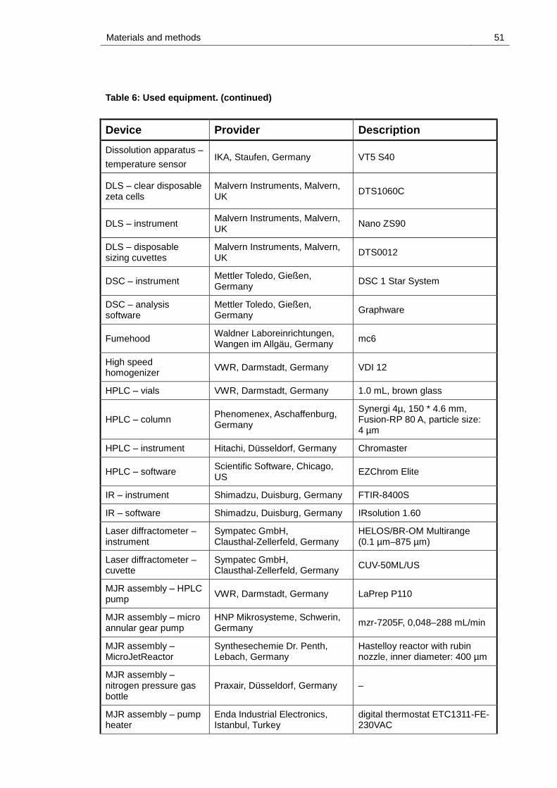
Materials and methods 51

Table 6: Used equipment. (continued)

Device Provider Description

Dissolution apparatus –

temperature sensor IKA, Staufen, Germany VT5 S40

DLS – clear disposable zeta cells

Malvern Instruments, Malvern, UK

DTS1060C

DLS – instrument Malvern Instruments, Malvern, UK

Nano ZS90

DLS – disposable sizing cuvettes

Malvern Instruments, Malvern, UK

DTS0012

DSC – instrument Mettler Toledo, Gießen, Germany

DSC 1 Star System

DSC – analysis software

Mettler Toledo, Gießen, Germany

Graphware

Fumehood Waldner Laboreinrichtungen, Wangen im Allgäu, Germany

mc6

High speed homogenizer

VWR, Darmstadt, Germany VDI 12

HPLC – vials VWR, Darmstadt, Germany 1.0 mL, brown glass

HPLC – column Phenomenex, Aschaffenburg, Germany

Synergi 4µ, 150 * 4.6 mm, Fusion-RP 80 A, particle size: 4 µm

HPLC – instrument Hitachi, Düsseldorf, Germany Chromaster

HPLC – software Scientific Software, Chicago, US

EZChrom Elite

IR – instrument Shimadzu, Duisburg, Germany FTIR-8400S

IR – software Shimadzu, Duisburg, Germany IRsolution 1.60

Laser diffractometer – instrument

Sympatec GmbH, Clausthal-Zellerfeld, Germany

HELOS/BR-OM Multirange (0.1 µm–875 µm)

Laser diffractometer – cuvette

Sympatec GmbH, Clausthal-Zellerfeld, Germany

CUV-50ML/US

MJR assembly – HPLC pump

VWR, Darmstadt, Germany LaPrep P110

MJR assembly – micro annular gear pump

HNP Mikrosysteme, Schwerin, Germany

mzr-7205F, 0,048–288 mL/min

MJR assembly –MicroJetReactor

Synthesechemie Dr. Penth, Lebach, Germany

Hastelloy reactor with rubin nozzle, inner diameter: 400 µm

MJR assembly – nitrogen pressure gas bottle

Praxair, Düsseldorf, Germany –

MJR assembly – pump heater

Enda Industrial Electronics, Istanbul, Turkey

digital thermostat ETC1311-FE-230VAC

52 Materials and methods

Table 6: Used equipment. (continued)

Device Provider Description

MJR assembly – water bath

VWR, Darmstadt, Germany VWB 6

pH meter Mettler Toledo, Gießen, Germany

Seven Multi S40

Rotary evaporator VWR, Darmstadt, Germany IKA RV 10 digital

SEM – instrument Carl Zeiss Microscopy, Oberkochen, Germany

EVO HD15

SEM – sputter coater Quorum, East Grinstead, UK Q150R ES

SEM – image analysis software

National Institutes of Health, Bethesda, US

ImageJ

Spreadsheet software Microsoft, Redmond, US Excel 2010

Ultrasonic bath VWR, Darmstadt, Germany USC300TH

UV-Vis –cuvette Hellma Analytics, Müllheim,Germany

101-QS, 10x10 mm, quartz

UV-Vis – instrument VWR, Darmstadt, Germany UV/VIS-1600PC

Materials and methods 53

The used chemical reagents are listed in Table 7 and were used as received.

Table 7: Chemical reagents.

Reagent Provider Description

Celecoxib Fraken Biochem,

Qingdao, China

CAS: 169590-42-5, MW: 381, batch: 201108054

Cetrimide Sigma Aldrich, Munich, Germany

CAS: 9004-34-6, MW: 364, hexadecyltrimethyammonium-

bromide ≥ 98%, batch: SLBC8213V

Distilled water Siemens, Munich, Germany CAS: 7732-18-5, MW: 18, prepared with: LaboStar 3 TWF-DI/-UV

Ethyl acetate VWR, Darmstadt, Germany CAS: 141-78-6, MW: 88, analytical grade

Eudragit E 100 Evonik Industries, Essen,

Germany

CAS: 24938-16-7, MW: ~47,000, poly(butyl methacrylate-co-(2-dimethylaminoeethyl)methylate-co-methylmethacrylate) 1:2:1, batch: E080501129

Hydrochloric acid, 37 %

Universität des Saarlandes–Zentrales Chemikalienlager, Saarbrücken, Germany

CAS: 7647-01-0, MW: 36

Methanol VWR, Darmstadt, Germany CAS: 67-56-1, MW: 32, HPLC grade

Phosphoric acid

VWR, Darmstadt, Germany CAS: 7664-38-2, MW: 98, batch: 10F240536, orthophosphoric acid 85%

Poloxamer 407 VWR, Darmstadt, Germany

CAS: 9003-11-6, MW: 1200, Pluronic F-127, polyoxypropylene polyoxyethylene co- polymer, batch: BCBC6633

Polyvinyl alcohol

Sigma Aldrich, Munich,

Germany

CAS: 9002-89-5, MW: ~27,000, Mowiol 4-98, Lot#BCBD5639V

Potassium dihydrogen phosphate

VWR, Darmstadt, Germany CAS: 7778-77-0, MW: 136, batch: 10H230005

Sodium chloride

VWR, Darmstadt, Germany CAS: 7647-14-5, MW: 58, batch: 10J11040

Sodium dodecyl sulfate

VWR, Darmstadt, Germany CAS: 151-21-3, MW: 288, batch: K41859334

Sodium hydroxide

VWR, Darmstadt, Germany CAS: 1310-73-2 , MW: 40, batch: 13B050037

54 Materials and methods

The used dissolution media are listed in Table 8.

Table 8: Dissolution media.

Dissolution medium Preparation

HCl pH 1.2 8.00 mL of hydrochloric acid, 37 % are diluted to 1000 mL with distilled water and the pH adjusted to 1.2 ± 0.05 with hydrochloric acid, 37 %

HCl pH 1.2 + 0.15 M NaCl 8.77 g of sodium chloride are dissolved in 1000 mL of HCl pH 1.2

HCl pH 1.2 +

0.001/0.01/0.05/0.3/1.0 %

cetrimide

0.010/0.10/0.50/3.0/10.0 g of cetrimide are dissolved in 1000 mL of HCl pH 1.2

0.02 M Phosphate buffer solution

pH 5.2 + 0.3 % cetrimide

2.72 g of potassium dihydrogen phosphate and 3.0 g of cetrimide are dissolved in 1000 ml of distilled water. The pH of the solution is 5.2 ± 0.05

0.05 M phosphate buffer

solution pH 4.5 + 0.3 %

cetrimide

6.80 g of potassium dihydrogen phosphate and 3.0 g of cetrimide are dissolved in 1000 ml of distilled water. The pH of the solution is adjusted with phosphoric acid to 4.5 ± 0.05

0.5 M Phosphate buffer solution

pH 3.5 + 0.3 % cetrimide

68.0 g of potassium dihydrogen phosphate and 3.0 g of cetrimide are dissolved in 1000 ml of distilled water. The pH of the solution is adjusted with phosphoric acid to 3.5 ± 0.05

0.73 M Phosphate buffer solution

pH 2.5 + 0.3 % cetrimide

100.0 g of potassium dihydrogen phosphate and 3.0 g of cetrimide are dissolved in 1000 ml of distilled water. The pH of the solution is adjusted with hydrochloric acid to 2.5 ± 0.05

0.73 M Phosphate buffer solution

pH 2.0 + 0.3 % cetrimide

100.0 g of potassium dihydrogen phosphate and 3.0 g of cetrimide are dissolved in 1000 ml of distilled water. The pH of the solution is adjusted with hydrochloric acid to 2.0 ± 0.05

Materials and methods 55

2.2 Methods

2.2.1 Nanoparticle preparation

2.2.1.1 Bench-top

First, a solution of celecoxib (5–100 mg/mL) and Eudragit E 100

(10–200 mg/mL) in ethyl acetate (1–5 mL) was poured into 10 mL of an

aqueous solution of PVA, SDS or Poloxamer 407 (0.01–5.0 % w/v). The

resulting emulsion was agitated three times for 30 s each using a high speed

homogenizer (see Table 6) at 30,000 rpm. Time intervals of 30 s were left

after the first and the second homogenization step. Then, ethyl acetate was

evaporated under vacuum. The manufacturing process is depicted

schematically in Figure 21. The resulting nanosuspensions were used

without further processing.

Figure 21: NP preparation procedure (bench top/emulsification-solvent evaporation).

56 Materials and methods

2.2.1.2 MicroJetReactor

Celecoxib (2.5 %) and Eudragit E 100 (5.0 %) were dissolved together in

ethyl acetate (emulsification-diffusion) or methanol (nanoprecipitation). Non-

solvent was an aqueous solution of Poloxamer 407 (1.25 %). The solvent jet

speed was varied between 100 and 1200 rpm by micro annular gear pumps,

while the non-solvent jet speed was respectively five times higher. The flow

rates corresponding to the respective pump rotational speed are stated in

Table 9. The operation temperature (water bath and pump heaters) was

chosen between 25 and 60 °C and the solutions equilibrated to the

respective temperature in the water bath prior to preparation. The nitrogen

flow was varied between 0 and 0.5 bar. For the setting 0 bar the nitrogen

access on top of the reactor was closed to prevent liquid flow into the gas

channel. The yielded suspensions were collected and remaining organic

solvent evaporated at ambient conditions.

Table 9: Flow rates of MJR assembly – micro annular gear pump at selected rotational

speeds (manufacturer specification).

The previous MJR preparation methods were applied for the studies

described in chapters 3.1, 3.2 (except of AFM characterization, see 3.2.4)

and 3.3.2 (Dissolution behavior of differently-sized NPs). The NPs used for

the dissolution studies described in chapter 3.3.1 were prepared with an

alternative method. Hence, preparative HPLC pumps (without pump heaters)

were used instead of micro annular gear pumps, while the remaining design,

including the reactor part, complies with the MJR assembly depicted in

Figure 10. This setup did not allow precise adjustment of nitrogen pressure.

Pump rotational speed

/rpm

Flow rate

/mL*min-1

300 14.4

750 36

1200 57.6

1500 72

3750 180

6000 288

Materials and methods 57

The preparation technique was nanoprecipitation (solvent: methanol). A co-

stabilizer (like Poloxamer 407) was not used. By this means white turbid

solutions were obtained and poured in polypropylene storage tubes. To

remove excessive methanol the tubes were opened and put in an operating

fumehood for approximately 18 h at ambient temperature. Table 10

summarizes the preparation details. With this method small NPs of narrow

size distribution can be obtained (see Table 16). Furthermore, it is not

necessary to use of a co-stabilizer and the energy-consumption (heating and

pumping energy) is lower. Though, this method does not facilitate the

production of NPs in a larger size range. Moreover the throughput of the first

method is much higher (maximum flow rates 288 mL/min versus 50 mL/min),

which is a decisive advantage for transfer to industry.

Table 10: Technical parameters of MJR preparation of celecoxib-Eudragit E 100-NPs

by nanoprecipitation – alternative method (without use of co-stabilizer).

Parameter Details

Solvent methanol

Non-solvent water

API celecoxib

Polymer Eudragit E 100

API concentration in solvent 4 mg/mL

Polymer concentration in non-solvent 8 mg/mL

Solvent flow rate 50 mL/min

Non-solvent flow rate 50 mL/min

Temperature (water bath) 25 °C

Nitrogen pressure approximately 0-0.5 bar

58 Materials and methods

2.2.2 Nanoparticle characterization

2.2.2.1 Dynamic light scattering

To determine Z-Average, PDI and ZP the nanosuspensions were diluted with

distilled water to a final concentration of 10-1–10-3 % (weight percentage of

celecoxib + Eudragit E 100) and transferred to a disposable sizing cuvette or

a zeta cell for measurement. This dilution factor is a compromise as, on one

hand, the used instrument requires a certain dilution to be able to measure

properly, whereas on the other hand, the dilution factor should be lower than

10-2–10-4 [148]. Prior to measurement samples were allowed to equilibrate in

the apparatus for 1 min at 25 °C. ZP was calculated using the Smoluchowski

equation [146]. Each measurement was performed in triplicate and the

arithmetic mean calculated.

2.2.2.2 Entrapment efficiency

Entrapment efficiency of NPs was determined by HPLC. Based on a

procedure from Baboota et al. [10] a HPLC method for the analysis of

celecoxib in aqueous media was developed. After adaption of the eluent

composition a sharp and symmetric peak was obtained at a retention time of

4.2 min. The HPLC parameters are summarized in Table 11. Linearity was

evaluated through injection of five celecoxib solutions (1–50 µg/mL) in mobile

phase. The correlation of the calibration curve was 0.9995.

Materials and methods 59

Table 11: HPLC method parameters for the determination of celecoxib content in NPs.

Parameter Details

Column Synergi Fusion-RP C-12, 4 µm, 150 * 4.6 mm

Column oven temperature 25 °C

Detector wavelength 250 nm

Elution system isocratic

Flow rate 1 mL/min

Injection volume 20 µL

Mobile phase methanol : water 73 : 27 (v/v)

Standard solution celecoxib 25 µg/mL in mobile phase

An aliquot of the respective nanosuspension was centrifuged for 30 min at

57950 g. The supernatant was carefully removed, appropriately diluted with

mobile phase and applied to HPLC. To remove excessive celecoxib and co-

stabilizer the residue was washed with water, the centrifugation step

repeated, the supernatant removed and the residue dried at ambient

conditions. Then, methanol was given to the pellet followed by 60 min

ultrasonication to ascertain complete dissolution. The obtained solution was

appropriately diluted with mobile phase and applied to HPLC. The EE was

calculated from equation (17),

EE =crf

c0*100 % (17)

where cr is the measured celecoxib concentration in dissolved residue, c0 the

total celecoxib concentration (content of residue and supernatant) and f the

dilution factor.

60 Materials and methods

2.2.2.3 Differential scanning calorimetry

10 ± 0.5 mg of each sample (celecoxib: 5 ± 0.5 mg) were sealed in pierced

aluminium pans of 40 µL. To obtain dry NP samples, aliquots of the

respective nanosuspensions were centrifuged and washed. After removal of

the supernatant they were dried for 24 h at ambient temperature. The

measurements were done at a scanning speed of 10 K/min from 298 up to

463 K with 80 mL/min of nitrogen purge.

2.2.2.4 Infrared spectroscopy

Approximately 10 mg of each sample were put on the diamond ATR crystal

and firmly pressed against it. For the preparation of the NP samples see

chapter 2.2.2.3. Celecoxib sodium and protonated Eudragit E 100 were

prepared by adding respectively 10 mL of either sodium hydroxide or

hydrochloric acid solution to equimolar amounts of celecoxib and

Eudragit E 100. Then, the liquid was evaporated under stirring at ambient

conditions followed by two washing steps with methanol to remove excessive

celecoxib or Eudragit E 100. The samples were scanned at wave numbers

ranging from 600 to 4000 cm-1 with a resolution of 4.0 cm-1.

2.2.2.5 Scanning electron microscopy

10 µL of a 1:100 aqueous dilution of each nanosuspension was mounted

onto a specimen stub and 24 h incubated at ambient conditions to evaporate

the liquid. Thereafter, the samples were sputtered with gold at 20 mA for 50 s

in order to prevent charging effects (layer thickness approximately 15 nm).

SEM imaging was carried out under high vacuum at ambient temperature

and an acceleration voltage of 10 kV. The secondary electron emission was

recorded using an Everhart-Thornley detector. To determine the particle size

an image analysis software (see Table 6) was used. Hereby, 20 particles

were randomly selected and measured.

Materials and methods 61

2.2.2.6 Atomic force microscopy

Prior to the examination the nanosuspensions were 1:10 diluted with distilled

water. A drop of each of these dilutions was placed on a freshly cleaved mica

sheet, respectively. Then, the mica sheet was dried for 24 h at ambient

conditions to evaporate the liquid. The AFM imaging was performed under

atmospheric conditions with a standard non-contact mode cantilever in

tapping mode at scan rates of 0.6 Hz.

62 Materials and methods

2.2.3 Dissolution tests

2.2.3.1 Verification of cross-flow filtration

Prior to the performance of dissolution tests with the nanosuspensions the

suitability of the used cross-flow filtration modules (see Table 6) was verified.

The modules (see Figure 22: schematic(a), photograph(b)) consist of a

hollow shaft, which contains several hollow fibers. The shaft has two side

ports, an inlet on the top and an outlet at the bottom. The inlet and the outlet

are sealed, except of the openings of the hollow fibers. As these fibers have

pores, which are permeable for substances below the size of 100 kDa

(MWCO: 10 nm) respectively 500 kDa (MWCO: 50 nm), they represent the

actual filtration system (this is depicted in the enlargement of Figure 22 (a)).

The dissolution medium with undissolved NPs and the dissolved API passes

the hollow fibers from the inlet to the outlet (the complete liquid circulation

from the beaker over the pump to the CF-module is shown in Figure 25).

Ideally, NPs shall be retained and liquid with dissolved API (filtrate)

penetrates the filter pores to the cavity between the fibers and the wall of the

shaft. Then, from the lower side port, filtrate can be collected and applied to

analysis. For the dissolution tests the upper side port has no function and is

closed with a Luer-Lok cap (this is shown in the photograph Figure 22 (b)).

The relevant properties of the cross-flow filtration modules are listed in Table

12.

Materials and methods 63

Table 12: Properties of the used cross-flow filtration modules.

Parameter Details

MWCO 10 nm (100 kDa CF module)

50 nm (500 kDa CF module)

Fiber inner diameter 0.5 mm

Fiber material modified polyether sulfone

Number of fibers 5-6

Filter surface area 20 cm2

Effective length 20 cm

Total length 23 cm

Housing inner diameter 3.1 mm

Housing outer diameter 4.6 mm

Inlet/retentate inner diameter 3 mm

In/out ports Male Luer-Lok

Side port Female Luer-Lok

64 Materials and methods

Figure 22: Cross-flow filtration module: Schematic of a MicroKros filter module (image

derived from http://eu.spectrumlabs.com/filtration/MicroKros.html?xfr=1373374033;)

with an enlargement of the hollow fibers (a) and photograph of this module as used in

the dissolution apparatus (b).

Materials and methods 65

As proof of principle the absence of NPs in the filtrate must be shown.

Thereto, celecoxib Eudragit E 100 NPs were prepared with MJR method

(alternative method, without usage of a surfactant, see chapter 2.2.1.2). The

volume-weighted size distribution of these particles is depicted in Figure 23

(a) (Z-Average: 143 nm, PDI: 0.237). Approximately 20 mL of this

nanosuspension passed along the hollow fibers of the filtration module using

the peristaltic pump. A DLS measurement of the filtrate was done. According

to the obtained result (see Figure 23 (b)) the filtrate does not contain NPs in a

significant amount, although this measurement was taken without previous

dilution while a 1 : 20 aqueous dilution was prepared for measurement of the

unfiltered nanosuspension. The peak one (0.78 nm) in Figure 23 (b) is near

to the lower measuring limit (0.3 nm) of the used DLS instrument. It can be

attributed to dissolved molecules of celecoxib or Eudragit E 100. Most

remarkable is the nearly complete absence of the distribution curve between

approximately 40 and 1000 nm. Figure 24 shows the results of the same test,

which was done with a 500 kDa CF-module. Hence, a 1 : 100 dilution of

another nanosuspension was measured versus the undiluted filtrate. The

result is comparable to the other experiment and reveals that > 99 % of the

NPs are retained by the filter.

As second test to verify the filter function, the UV absorbance of both

nanosuspension and filtrate (respectively 1 : 100 aqueous dilution) was

measured (λ = 252 nm). Hence, the nanosuspension showed a strong

absorbance (~ 1.8) whereas the filtrate absorbance was nearly zero (data not

shown). Thus, the suitability of the cross-flow filtration module for the

separation of polymer NPs was demonstrated.

The DLS verification test was successfully repeated for every CF-module

(100 kDa and 500 kDa) prior to use.

66 Materials and methods

Figure 23: DLS size distribution reports (volume-weighted) of a celecoxib-

Eudragit E 100 aqueous nanosuspension; NP-preparation: nanoprecipitation

technique–alternative method using HPLC pumps and a non-solvent phase without

surfactant (see chapter 2.2.1.2); unfiltered nanosuspension (1 : 20 dilution in water) (a)

versus liquid obtained from filtration of this nanosuspension through a 100 kDa CF

module (b); NP properties: 143 nm (Z-Average), 0.237 (PDI).

Materials and methods 67

Figure 24: DLS size distribution reports (volume-weighted) of a celecoxib-

Eudragit E 100 aqueous nanosuspension; NP-preparation: nanoprecipitation

technique–alternative method using HPLC pumps and a non-solvent phase without

surfactant (see chapter 2.2.1.2); unfiltered nanosuspension (1 : 100 dilution in water)

(a) versus liquid obtained from filtration of this nanosuspension through a 500 kDa CF

module (b); NP properties: 216 nm (Z-Average), 0.108 (PDI).

68 Materials and methods

2.2.3.2 Dissolution test methodology

The conduction of drug release tests of nanosuspensions involving cross-

flow filtration required the development of an individual experimental setup.

Figure 25 shows photographs of the complete assembly (a), the filtrate outlet

(b) and the sample withdrawal (c). A 150 mL-beaker, containing 99–99.75 mL

of dissolution medium and a cylindrical magnetic bar (length: 1.2 cm,

diameter: 0.45 cm), were put onto a magnetic stirrer. The temperature sensor

of the magnetic stirrer was attached to the magnetic stirrer and dived to a

depth of circa 2 cm into the dissolution medium to maintain a temperature of

37 ± 0.5 °C throughout the complete experiment. The rotational speed was

set to 300 rpm. The beaker was covered with plastic paraffin film to prevent

evaporation of the medium (loss of medium after 120 min at 37 °C and

stirring at 300 rpm: without cover ~ 3–4 mL, with cover < 1 mL).

To start the dissolution test 0.25–1 mL of the respective nano- or API

powder-suspension were given into the medium. The API powder sample

was prepared by suspending celecoxib to a concentration of 4 mg/mL in

water. Immediately prior to the test this suspension was ultrasonicated for

2 min followed by manual shaking for 30 s to avoid the formation of

agglomerates. For sample withdrawal a rubber hose was inserted into the

medium and the liquid aspirated by a peristaltic pump, which was operated

throughout the complete experiment. Then, before being returned to the

beaker, the medium passed the CF-module. From the lower open end at the

side of the module up to 2.0 mL of filtered liquid were collected with a

polypropylene reaction tube at every sampling point and applied to UV-Vis

API analysis. After each sampling the collected volume was replaced with

fresh medium.

After the experiment the filtration module was carefully rinsed with 0.1 M

sodium hydroxide followed by distilled water. For storage the modules were

emptied and the openings closed.

Materials and methods 69

Fig

ure

25: P

ho

tog

rap

h o

f the d

isso

lutio

n te

st a

ss

em

bly

(a), w

ith im

ag

e d

eta

ils o

f the filtra

te o

utle

t (b) a

nd

the s

am

ple

with

dra

wal (c

).

70 Materials and methods

2.2.3.3 Dead-end filtration

To compare the performance of the CF setup to conventional approaches

implementing dead-end filters, the samples were withdrawn from the beaker

using disposable syringes instead of aspiration with the peristaltic pump.

Thereto, 30 s prior to the defined sampling timepoint 5 mL of dissolution

medium were withdrawn and given back to the beaker immediately as

washing step of the filter. At the sampling timepoint the syringe was filled

again with the same volume, a 0.2 µm syringe filter holder attached and 2 mL

of liquid transferred through the filter. Then, the filter was removed from the

syringe, the remaining liquid given back to the beaker and the collected

volume replaced with fresh medium, which was previously equilibrated to

37 °C.

2.2.3.4 Flow properties

According to the specification of the used peristaltic pump the flow rate can

be varied between 0.8 and 105 mL/min. In combination with the used

Pharmed BPT tubes, this corresponds to pressure values between

approximately 0.01 and 2 bar. To examine the flow-through performance of

the complete system (permeate and retentate flow) the arrangement was

prepared as described in chapter 2.2.3.2 with the exception that a second

beaker was used to collect liquid from the respective outlets. Then, the first

beaker was filled with distilled water and attached to the pump, which was

operated at maximum speed. The water from both outlets was collected for

60 s and the amount weighed.

A second experiment was conducted to examine the permeation rate. Hence,

the water volume from the lower side outlet of the module (filtrate outlet) was

collected for 10 s at maximum pump speed. Additionally, the time span

between turning on of the pump and the first appearance of water at the side

outlet (dead time) was determined. All trials were performed in triplicate

(results listed in Table 13).

Materials and methods 71

Table 13: Flow-through properties of the cross-flow filtration system (permeate plus

retentate and permeate), n=3, values are mean ± SD.

Outlet Permeate and retentate Permeate

Water volume collected

/mL

131.7 ± 0.9 (after 60 s) 1.75 ± 0.035 (after 10 s)

Flow-through /mL*min-1

131.7 10.5

Dead time /s n/a 12.7 ± 0.6

The results reveal that the flow-through rate is with a value of 131.7 mL/min

even above the specification (105 mL/min). Provided that the used volume of

the dissolution medium is approximately 100 mL more than the complete

content of the beaker passes the CF-membrane in less than one minute.

Though, since pharmaceutical compendia demand the withdrawal of

specimen within a limited time span, the more important value is the

permeation rate. To gather 2 mL of filtrate for analysis circa 11.4 s are

required considering the above obtained results. For instance, after 1 min this

represents a deviation of 19.2 %. The USP allows a tolerance of only ± 2 %

at the stated sampling time [150].

However, it is to consider that this regulation applies to conventional

withdrawal of a specimen if one uses USP Apparatus 1 (Basket) or 2

(Paddle). Hence, the specimen is withdrawn in a single drawing operation

with a syringe. In detail, this means that the timepoint of withdrawal

corresponds to the current status of drug release. Conversely, using the CF

system, the specimen is collected over a certain period, analogously to USP

Apparatus 4 (Flow-Through Cell). In this context, the sampling period will

include the timepoint of interest. Thus, provided that the dissolution process

is linear within the respective range, the measured concentration of dissolved

API will be that of the center of the period. Under these circumstances, the

filtrate collection time may exceed the compendial tolerance.

Furthermore, it was observed during conduction of the dissolution tests that

the filtration rate also depends on the individual properties of the used

72 Materials and methods

dissolution medium. Hence, the usage of a surfactant decelerated the filtrate

flow rate by factor two to three, depending on the concentration. This was

compensated through individual adaption of start and end point of sampling.

Finally, it must be stated that the experimental value of the sampling points

does not correspond to the respective value since the dead time has to be

added. Though, this is the same difference for each dissolution test.

2.2.3.5 API quantification

As a less time-consuming alternative compared to HPLC, UV-Vis

spectroscopy was applied to quantify celecoxib in the filtrate. For verification

of the method specificity, spectra of methanolic solutions of celecoxib,

Eudragit E 100 and Poloxamer 407 were taken over a wavelength range from

190 to 400 nm (data not shown). Poloxamer 407 did not show UV

absorbance over the investigated range. A local absorbance maximum of

celecoxib, which was not significantly affected by Eudragit E 100

absorbance, was found at 252 nm.

For determination of the linearity a methanolic solution of celecoxib (without

additives) was prepared (c = 1 mg/mL). This solution was respectively diluted

to three different concentrations with the currently used dissolution medium.

These concentrations covered the range resulting from the dissolution

experiments. Then, a spectrum of the highest concentrated dilution was

recorded to detect the respective absorbance maximum (248–255 nm). In

every case calibration yielded a correlation of 0.999 or more. Thus, UV-Vis

spectroscopy was considered to be appropriate for quantification of celecoxib

in presence of Eudragit E 100 and Poloxamer 407. Additionally, this is in

good agreement with literature [2].

To determine the celecoxib concentration of the tested nanosuspensions

corresponding to 100 % API release, six aliquots of the suspension were

dissolved in methanol. These mixtures were appropriately diluted with the

respective dissolution medium for measurement. Thereafter, the dilutions

were applied to analysis. In the results part the degree of dissolution is given

Materials and methods 73

as percentage of this concentration considering the dilution factor of the

suspension in the medium.

2.2.3.6 Statistical evaluation of dissolution profile equivalence

The statistical comparison of dissolution profiles of differently-sized

celecoxib-Eudragit E 100-NPs and celecoxib (API) powder was performed

under application of the model independent approach according to FDA

“Guidance for Industry: Dissolution Testing of Immediate Release Solid Oral

Dosage Forms” [153]. This approach implements the calculation of a

difference factor f1 and a similarity factor f2, while the respective results

confirm or deny equivalence of two curves.

The difference factor (f1) which is a measurement of the relative error

between the two curves is calculated from equation (18),

f1 = {[∑ |Rt − Tt|n

t=1] / [∑ Rt

n

t=1]} ∙100 (18)

where n is the number of time points and Rt and Tt are the respective

dissolution values of the two compared curve at time t. In this study, the

points at 20, 40 and 60 s have been used for evaluation.

The similarity factor (f2) is a measurement of the similarity in percentage

dissolution between the two curves and is calculated from equation (19).

f2 = 50 ∙ {log [1+ ( 1 n) ∑ (Rt − Tt)2

n

t=1⁄ ]

-0,5

∙ 100} (19)

Two dissolution profiles were considered to be equivalent if f1 values were

between 0–15 and f2 values between 50–100.

74 Results

3 Results

3.1 Nanoparticle preparation

3.1.1 Bench-top

3.1.1.1 Influence of type of co-stabilizer, solvent : non-solvent ratio and

drug : polymer ratio

To optimize the bench-top preparation of celecoxib-Eudragit E 100-NPs, type

of co-stabilizer, solvent : non-solvent ratio and drug : polymer ratio were

varied and the effect on Z-Average, PDI, ZP and EE investigated.

Thereto, three different stabilizers (Poloxamer 407, PVA and SDS) were

respectively dissolved to a concentration of 0.1 % (w/v) in the non-solvent

phase. Furthermore, celecoxib : Eudragit E 100 ratios (w/w) of 1 : 1 and 1 : 2

and solvent : non-solvent ratios (v/v) of 1 : 2, 1 : 5 and 1 : 10 were examined.

Hence, stabilization with Poloxamer 407 resulted in NP diameters from

approximately 270 to 370 nm with PDI values in the range from 0.1 to 0.2, a

ZP from circa 45 to 60 mV and an EE between 62 and 90 %. At

solvent : non-solvent ratios of 1 : 5 and 1 : 10 no agglomerates appeared,

neither instantaneous nor after 24 h, while slight agglomeration occurred at

the 1 : 2 ratio. These results are graphically depicted in Figure 26 and the

data given in Table 19. Figure 27 shows the volume-weighted DLS size

distribution report of the nanosuspension prepared with 1 : 5 solvent : non-

solvent ratio and 1 : 2 celecoxib : Eudragit E 100 ratio.

Results 75

Figure 26: Bench-top preparation (emulsification-diffusion) of celecoxib-

Eudragit E 100 – NPs with Poloxamer 407 as co-stabilizer, (a) Z-Average and PDI, (b)

ZP and EE: Solvent phase: 5 mg/mL celecoxib and 5/10 mg/mL Eudragit E 100 in

1/2/5 mL of ethyl acetate, non-solvent phase: 1 mg/mL Poloxamer 407 in 10 mL of

water, n=1, Z-Average, PDI and ZP values are mean of three measurements, EE values

respectively single measurement, red lines represent SD.

76 Results

Figure 27: DLS size distribution report (volume-weighted) of celecoxib-Eudragit E 100

– NPs with Poloxamer 407 as co-stabilizer: Solvent phase: 5 mg/mL celecoxib and

10 mg/mL Eudragit E 100 in 2 mL of ethyl acetate, non-solvent phase: 1 mg/mL

Poloxamer 407 in 10 mL of water; Preparation method: Bench-top (emulsification-

diffusion).

Results 77

Using SDS, particles between approximately 200 and 7200 nm diameter, PDI

values between 0.03 and 0.67, a ZP from circa -10 to 50 mV and EEs from

55 to 90 % were obtained. In every sample of this setup agglomeration

occurred directly after preparation. The particles prepared with a 1 : 2

solvent : non-solvent ratio completely agglomerated after 24 h storage at

ambient temperature.

With PVA the particle diameter ranged from about 270 nm to large

microparticles with PDI values between 0.5 and 1.0 and a ZP between -4 and

12 mV. The EE did not exceed 1 %. The suspensions exclusively contained

agglomerates.

These results are listed in the appendix (SDS Table 20, PVA Table 21).

78 Results

3.1.1.2 Influence of Poloxamer 407 (co-stabilizer) concentration

To elaborate the influence of Poloxamer 407, it was dissolved to different

concentrations (0.1-10 mg/mL) in water as non-solvent phase, while the

solvent phase was prepared according to the previously elaborated

conditions (see chapter 3.1.1.1). The results of this experimental setup are

listed in Table 22 and shown in Figure 28. Figure 29 shows the volume-

weighted DLS size distribution report of one nanosuspension prepared with

2.5 mg/mL of Poloxamer 407 in non-solvent phase.

The resulting NP diameters decreased with increasing stabilizer

concentration from more than 400 nm at 0.1 mg/mL to slightly more than

200 nm at 2.5 mg/mL which basically remained constant at higher

concentrations. The PDI values were between 0.25 and 0.30 for 0.1 mg/mL

and 0.5 mg/mL, at approximately 0.15 for 1 mg/mL and at 0.05 or slightly

below at the higher concentrations. While the ZP values did not particularly

differ from 0.1 mg/mL to 1 mg/mL (50 mV or slightly less), they decreased

over circa 40 mV at 2.5 mg/mL to around 30 mV at 5 mg/mL and 10 mg/mL.

The EE values decreased from 90 % to 50 % with increasing Poloxamer 407

concentration. Decreasing EE values were accompanied by increasing API

concentrations in the supernatant. In every case white, turbid suspensions

were yielded, while with 5 mg/mL and 10 mg/mL of Poloxamer 407 the color

tended to slightly bluish. Using 0.1 mg/mL, 0.5 mg/mL or 1 mg/mL sediments

appeared on the flask wall during evaporation.

Results 79

Figure 28: Bench-top preparation (emulsification-diffusion) of celecoxib

Eudragit E 100 – NPs with varying amounts of Poloxamer 407, (a) Z-Average and PDI,

(b) ZP and EE: Solvent phase: 5 mg/mL celecoxib and 10 mg/mL Eudragit E 100 in

2 mL of ethyl acetate, non-solvent phase:0.1/0.5/1/2.5/5/10 mg/mL Poloxamer 407 in

10 mL of water, n=3, red lines represent SD.

80 Results

Figure 29: DLS size distribution report (volume-weighted) of celecoxib-Eudragit E 100

– NPs with Poloxamer 407 as co-stabilizer: Solvent phase: 5 mg/mL celecoxib and

10 mg/mL Eudragit E 100 in 2 mL of ethyl acetate, non-solvent phase: 2.5 mg/mL

Poloxamer 407 in 10 mL of water; Preparation method: Bench-top (emulsification-

diffusion).

Results 81

3.1.1.3 Increase of celecoxib and excipients quantity

The celecoxib concentration in the solvent phase was increased from

5 mg/mL to 25, 50 and 100 mg/mL. Simultaneously the concentrations of

Eudragit E 100 and Poloxamer 407 were increased to maintain the previously

elaborated ratios. A celecoxib : Eudragit E 100 : Poloxamer 407 ratio of

1 : 2 : 0.025 was once employed to examine the influence of a very low co-

stabilizer concentration at relatively high celecoxib amount. Then, the effect

on NP size, PDI, ZP and EE was investigated. The results of these

experiments are listed in Table 14. Both formulations produced with 100 mg

celecoxib agglomerated already during the preparation process and solidified

after 24 h storage at ambient conditions. With a Poloxamer 407 concentration

of 2.5 mg/mL and 50 mg/mL the Z-Average was 810 ± 126 nm and

1002 ± 261 nm, the ZP 53 ± 1 mV and 34 ± 1 mV and the EE (HPLC) circa

97 % and 86 %, respectively. The PDI was 1 in both cases. The usage of

50 mg celecoxib likewise resulted in agglomeration, while the Z-Average was

579 ± 66 nm, the PDI was 1, the ZP 37 ± 1 mV and the EE (HPLC)

approximately 80 %. With the lowest tested celecoxib concentration

(25 mg/mL), the Z-average was around 350 nm, the PDI was slightly below

0.1, the ZP was circa 36 mV and the EE circa 85 %. Figure 30 shows a

volume-weighted DLS size distribution report of this nanosuspension.

82 Results

Table 14: Bench-top preparation (emulsification-diffusion) of celecoxib-Eudragit E 100

– NPs with Poloxamer 407 as co-stabilizer. Solvent phase: 25/50/100 mg/mL celecoxib

and 50/100/200 mg/mL Eudragit E 100 in 2 mL ethyl acetate, non-solvent phase:

2.5/12.5/25/50 mg/mL Poloxamer 407 in 10 mL of water, 3 x 30 s homogenization at

30000 rpm, removal of ethyl acetate in rotary evaporator (5 min at 40 °C, 220 mbar and

280 rpm followed by 10 min at 40 °C, 180 mbar, and 280 rpm), n=3 (25 mg/mL

celecoxib, 50 mg/mL Eudragit E 100 and 12.5 mg/mL Poloxamer 407) and n=1 (other

formulations), n=1: Z-Average, PDI and ZP values are mean of three measurements ±

SD, EE values respectively single measurement, n=3: values are mean ± SD.

c(celecoxib) ; c(Eudragit E 100) /mg*mL-1

c

(Poloxamer 407)

/mg*mL-1

Visual

inspection

Z-Average

/nm

PDI ZP

/mV

EE

/%

25 ; 50 12.5 a 352 ± 6 0.09 ± 0

36 ± 0.3

85.3 ± 2.6

50 ; 100 25 b 579 ± 66 1 37 ±

1 79.5

100 ; 200 50 c 1002 ± 261 1 34 ±

1 85.7

100 ; 200 2.5 d 810 ± 126 1 53 ±

1 97.2

a: white, turbid liquid

b: slight agglomeration on the flask wall, white, turbid liquid

c: agglomeration on the flask wall, white, turbid liquid, sample entirely agglomerated after 24 h

d: strong agglomeration on the flask wall, white, turbid liquid, sample entirely agglomerated after 24 h

Results 83

Figure 30: DLS size distribution report (volume-weighted) of celecoxib-

Eudragit E 100 – NPs with Poloxamer 407 as co-stabilizer: Solvent phase: 25 mg/mL

celecoxib and 50 mg/mL Eudragit E 100 in 2 mL of ethyl acetate, non-solvent phase:

12.5 mg/mL Poloxamer 407 in 10 mL of water; Preparation method: Bench-top

(emulsification-diffusion).

84 Results

3.1.1.4 Stability study

To choose an appropriate formulation as template for optimization with MJR

technology the stability of the formulations containing 5 mg/mL (see

chapter 3.1.1.2) and 25 mg/mL (see chapter 3.1.1.3) celecoxib was

investigated over 28 d. Thereto, each formulation was prepared in triplicate

and respectively split into two parts to be stored at ambient temperature and

at 5 ± 2 °C. NP size, PDI, ZP and EE were determined on the day of

preparation and after 1, 2, 3, 4, 7 and 14 d storage. After 28 d all samples

had been crystallized (sharp needles on the container interior wall, clear

liquid). Figure 31 shows photographs of the formulations after preparation

(a), 7 d ((b) and (c)) and 28 d ((d), (e) and (f)). The results are listed in Table

23 (5 mg/mL celecoxib, storage at ambient temperature), Table 24 (5 mg/mL

celecoxib, storage at 5 °C), Table 25 (25 mg/mL celecoxib, storage at

ambient temperature) and Table 26 (25 mg/mL celecoxib, storage at 5 °C).

The results are graphically displayed in Figure 32 (Z-Average and PDI),

Figure 33 (ZP) and Figure 34 (EE).The results of the statistical evaluation

(t-tests for comparison of Z-Average, PDI, ZP and EE: storage at room

temperature versus storage at 5 °C and usage of 5 mg/mL versus 25 mg/mL

celecoxib in solvent phase) are stated in Table 27.

On the basis of a 95 % confidence interval the storage temperature (first

comparison) had no significant influence on the examined parameters.

Concerning the second comparison (between the two formulations) both

Z-Average and EE showed a significant difference if considering a storage

period of 14 d. Hence there also was a difference in PDI for those samples

being stored at room temperature.

The Z-Average after preparation was about 220 nm for the formulation with

low and about 290 nm for the formulation with high celecoxib content. From

days three to seven the Z-Average values increased while they were

constant for the formulation with high celecoxib content, which was stored at

ambient temperature.

The PDI was overall approximately 0.1 at the beginning and was likewise

constant for the formulation with high celecoxib content, which was stored at

ambient temperature. If this formulation was stored at 5 °C it increased to

Results 85

about 0.37 after 4 d. With low celecoxib content it changed to 0.15–0.16 after

2 d of storage and further increased thereafter regardless of the storage

conditions.

The ZP values were initially 39 ± 1 mV in every case. With low celecoxib

content they continuously increased over the storage period to about 56 mV

(RT) respectively 52 mV (5 °C). With high celecoxib content values reached

approximately 45 mV.

The EE values varied between circa 70 % and 80 % (formulations with low

celecoxib content) and between 80 % and 90 % (formulations with high

celecoxib content) without a trend. Thus, this parameter is obviously not

stability-related.

Figure 35 shows volume-weighted DLS size distribution reports of one

nanosuspension prepared with the higher celecoxib concentration

immediately after preparation and after 14 d of storage (RT).

86 Results

Fig

ure

31:

Ph

oto

gra

ph

s o

f cele

co

xib

-Eu

dra

git

E 1

00-N

Ps s

tab

iliz

ed

wit

h P

olo

xam

er

40

7, aft

er

pre

para

tio

n (

a),

7 d

at

am

bie

nt

tem

pe

ratu

re (

b),

7 d

at

5 °

C (

c),

28

d a

t am

bie

nt

tem

pera

ture

(d

), 2

8 d

at

5 °

C (

e)

an

d 2

8 d

at

5 °

C (

top

vie

w)

(f):

C =

cele

co

xib

, E

= E

ud

rag

it E

100,

P =

Po

loxam

er

407, R

T =

ro

om

/am

bie

nt

tem

pera

ture

.

Results 87

Fig

ure

32: S

tab

ility s

tud

y o

f cele

co

xib

-Eu

dra

git E

100 –

NP

s s

tab

ilized

with

Po

loxam

er 4

07 (Z

-Ave

rag

e a

nd

PD

I): So

lven

t ph

ase:

5/2

5 m

g/m

L c

ele

co

xib

an

d 1

0/5

0 m

g/m

L E

ud

rag

it E 1

00 in

2 m

L e

thyl a

ceta

te, n

on

-so

lven

t ph

as

e: 2

.5/1

2.5

mg

/mL

Po

lox

am

er 4

07 in

10 m

L w

ate

r, resp

ectiv

ely

sto

red

at ro

om

tem

pe

ratu

re (R

T) a

nd

at 5

°C, n

=3

, valu

es

are

me

an

of th

ree

measu

rem

en

ts, re

d lin

es

rep

resen

t SD

.

88 Results

Fig

ure

33:

Sta

bil

ity s

tud

y o

f cele

co

xib

-Eu

dra

git

E 1

00 –

NP

s s

tab

iliz

ed

wit

h P

olo

xam

er

40

7 (

ZP

): S

olv

en

t p

hase:

5/2

5 m

g/m

L

cele

co

xib

an

d 1

0/5

0 m

g/m

L E

ud

rag

it E

100 in

2 m

L e

thyl ac

eta

te, n

on

-so

lve

nt

ph

ase:

2.5

/12.5

mg

/mL

Po

loxam

er

407 i

n 1

0 m

L w

ate

r,

resp

ecti

vely

sto

red

at

roo

m t

em

pera

ture

(R

T)

an

d a

t 5

°C

, n

=3

, valu

es a

re m

ean

of

thre

e m

easu

rem

en

ts,

red

lin

es

rep

res

en

t S

D.

Results 89

Figure 34: Stability study of celecoxib-Eudragit E 100 – NPs stabilized with

Poloxamer 407 (EE), (a) 5 mg/mL celecoxib and (b) 25 mg/mL celecoxib: Solvent

phase: 5/25 mg/mL celecoxib and 10/50 mg/mL Eudragit E 100 in 2 mL ethyl acetate,

non-solvent phase: 2.5/12.5 mg/mL Poloxamer 407 in 10 mL water, respectively stored

at room temperature (RT) and at 5 °C, n=3, single measurements, red lines represent

SD.

90 Results

Figure 35: DLS size distribution reports (volume-weighted) of celecoxib-

Eudragit E 100 – NPs with Poloxamer 407 as co-stabilizer: Solvent phase: 25 mg/mL

celecoxib and 50 mg/mL Eudragit E 100 in 2 mL of ethyl acetate, non-solvent phase:

12.5 mg/mL Poloxamer 407 in 10 mL of water; immediately after preparation (day 0) (a)

and after two weeks storage at ambient temperature (day 14) (b); Preparation method:

Bench-top (emulsification-diffusion).

Results 91

3.1.2 MicroJetReactor

3.1.2.1 Emulsification-diffusion

Since stable NPs of narrow size distribution should be prepared in three

different sizes the MJR technology was applied (see chapter 2.2.1.2) based

on the elaborated formulation made with 25 mg/mL celecoxib and 50 mg/mL

Eudragit E 100 (see Table 28). To reduce the experimental effort DoE was

used. As independent variables temperature, nitrogen pressure and pump

rotational speed were chosen. Thereby, the effect on the Z-Average

(dependent variable) was investigated. According to findings from pre-

experiments (data not shown) the temperature was varied between 40 and

60 °C, the nitrogen pressure between 0 and 0.50 bar and the pump rotational

speed between 300 : 1500 and 1200 : 6000 rpm. In this way, NPs of

Z-Averages between 260 and 750 nm and of PDI values between 0.06 and 1

were yielded. The experimental setup and the corresponding results are

summarized in Table 28.

For the evaluation a response surface reduced quadratic model was chosen.

This model is significant due to a p-value of the fit function < 0.0001 and a

Model F-value of 65.80 (Program conclusion: “There is only a 0.01% chance

that a "Model F-Value" this large could occur due to noise...Values of "Prob >

F" [p-values] less than 0.0500 indicate model terms are significant. Values

greater than 0.1000 indicate the model terms are not significant.”). The

R-squared value is 0.9869. The design cube is shown in Figure 36. The

model is represented by equation (20) where A represents the operation

temperature, B the nitrogen pressure and C the rotational speed of the pump,

which carries the solvent.

Z-Average =

310.475 + (17.35 * A) - (22.575*B) - (57.5*C) −

(91.025*AC)+(158.125*BC) − (52.725*A2)+

(48.725*B2)+(130.875*C

2)

(20)

92 Results

Figure 36: Design cube (particle size) of the DoE model. Values at the cube edges

represent the Z-Average in nm (dependent variable). The x-axis (A) represents the

temperature (in °C), the y-axis (C) the flow rate (expressed as pump rotational speed

in rpm) and the z-axis (B) the nitrogen pressure (in bar).

Results 93

For the validation of the previously obtained DoE model solutions of equation

(20) were calculated for four different Z-Average values (300, 350, 400 and

450 nm). In addition to the Z-Average, PDI, ZP and EE were measured

(results stated in Table 29). The PDI values ranged from 0.08 to 0.22, the ZP

values were circa 45 ± 3 mV and the EE ranged from 81–91 %. The

Z-Average values corresponded to the predicted values with deviations of

less than 10 % except of one formulation (59.0 °C_0.36 bar_350 : 1750 rpm)

whose Z-Average differed 12.4 % from the predicted result. The actual

Z-Average values are plotted against the predicted values in Figure 37.

Hence, the R-squared value is 0.8792. Figure 38 shows the volume-weighted

DLS size distribution report of one nanosuspension with a predicted value of

350 nm.

Figure 37: Design of experiments – validation: Actual Z-Average values of ten

approaches in three sizes (300, 350, 400 and 450 nm) plotted against predicted values

obtained from DoE equation.

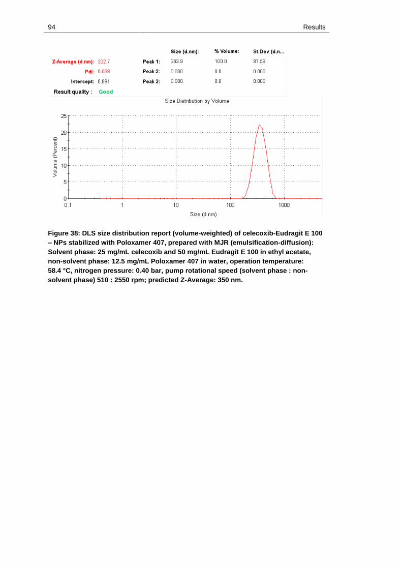
94 Results

Figure 38: DLS size distribution report (volume-weighted) of celecoxib-Eudragit E 100

– NPs stabilized with Poloxamer 407, prepared with MJR (emulsification-diffusion):

Solvent phase: 25 mg/mL celecoxib and 50 mg/mL Eudragit E 100 in ethyl acetate,

non-solvent phase: 12.5 mg/mL Poloxamer 407 in water, operation temperature:

58.4 °C, nitrogen pressure: 0.40 bar, pump rotational speed (solvent phase : non-

solvent phase) 510 : 2550 rpm; predicted Z-Average: 350 nm.

Results 95

3.1.2.2 Nanoprecipitation

As an alternative to the emulsification-diffusion method nanoprecipitation was

applied for the preparation of NPs. Thereto, methanol was employed as

solvent instead of ethyl acetate while the NP composition and preparation

were analogous to emulsification-diffusion. Concerning the MJR parameters

the nitrogen pressure was varied between 0 and 0.50 bar and the pump

rotational speed between 300 : 1500 and 1200 : 6000 rpm as previously (see

chapter 3.1.2.1). Contrary to emulsification-diffusion the temperature was set

to 30 or 50 °C since the boiling point of methanol (65 °C) is lower than that of

ethyl acetate (77 °C). The results are stated in Table 15. The Z-Average

values were mainly in a range between 300 and 500 nm at a PDI from 0.1 to

0.5 except of one setting (run 5) which led to strong agglomeration directly

after preparation (Z-Average: ~ 960 nm, PDI: ~ 1). The ZP values were

36 ± 3 mV throughout all settings. The EE was consistently higher if the

pump rotational speed was 300 : 1500 (~ 83–95 %), while using the ratio of

1200 : 6000 smaller values were obtained (~ 57–70 %) except of one setting

(run 3: ~ 83 %). Figure 39 shows the volume-weighted DLS size distribution

report of one of the prepared nanosuspensions.

96 Results

Table 15: MJR preparation of celecoxib-Eudragit E 100-NPs stabilized with

Poloxamer 407, nanoprecipitation technique: Solvent phase: 25 mg/mL celecoxib and

50 mg/mL Eudragit E 100 in methanol, non-solvent phase: 12.5 mg/mL Poloxamer 407

in water, operation temperature: 40 and 60 °C, nitrogen pressure: 0 and 0.5 bar, pump

rotational speed (solvent phase : non-solvent phase) 300 : 1500 rpm and 1200 :

6000 rpm, n=1, Z-Average, PDI and ZP values are mean of three measurements ± SD,

EE values respectively single measurement.

Run

Tempera-ture

/°C

Nitrogen pressure

/bar

Pump rotational speed

/rpm

Z-Average

/nm

PDI ZP

/mV

EE

/%

1 30.0 0.50 300 : 1500 416.9 ± 5.3 0.136

± 0.070

34.5 ± 0.7

94.9

2 50.0 0.50 300 : 1500 517.7 ±

35.8

0.178 ±

0.155

35.3 ± 0.252

85.7

3 30.0 0.50 1200 : 6000 384.7 ±

17.0

0.441 ±

0.026

33.3 ± 1.4

83.1

4 50.0 0.50 1200 : 6000 313.7 ±11.5 0.339

± 0.084

38.2 ± 0.7

56.9

5 30.0 0 300 : 1500 964.2 ± 180.8

0.993 ±

0.012

34.5 ± 0.6

87.1

6 50.0 0 300 : 1500 335.4 ± 9.3 0.482

± 0.076

37.2 ± 0.7

83.4

7 30.0 0 1200 : 6000 313.7 ±

10.3

0.362 ±

0.059

34.7 ± 0.6

70.3

8 50.0 0 1200 : 6000 321.9 ± 7.9 0.253

± 0.036

40.7 ± 0.6

64.1

Results 97

Figure 39: DLS size distribution report (volume-weighted) of celecoxib-Eudragit E 100

– NPs stabilized with Poloxamer 407, prepared with MJR (nanoprecipitation): Solvent

phase: 25 mg/mL celecoxib and 50 mg/mL Eudragit E 100 in methanol, non-solvent

phase: 12.5 mg/mL Poloxamer 407 in water, operation temperature: 50.0 °C, without

nitrogen, pump rotational speed (solvent phase : non-solvent phase) 1200 : 6000 rpm.

98 Results

3.2 Nanoparticle characterization

3.2.1 Differential scanning calorimetry

To elucidate the structure of the prepared NPs DSC measurements were

performed. Figure 40 shows DSC traces of celecoxib, Eudragit E 100, a

physical 1:2 mixture of celecoxib and Eudragit E 100 as well as celecoxib-

Eudragit E 100-NPs prepared by emulsification-diffusion and

nanoprecipitation technique.

The glass transition (Tg) of Eudragit E 100 was detected at circa 45 °C

(inflection point of the decline of the Eudragit E 100 trace between 33 °C and

58 °C) followed by a negative peak indicating enthalpy relaxation at 60 °C.

The celecoxib melting point (Tm) was at approximately 164 °C. In the physical

mixture the Eudragit E glass transition was shifted to circa 42 °C, while the

melting peak of celecoxib was bimodal with minima at 154 °C and 158 °C.

The NPs, which were prepared with the emulsification-diffusion technique,

showed a glass transition at 37 °C, while further distinct signals were

missing. Concerning the comparison of the two NP preparation methods

(nanoprecipitation and emulsification-diffusion) there was no difference in the

glass transition. However, the NPs, which were prepared by

nanoprecipitation, exhibited an additional broad signal from 96 °C to 160 °C,

which was attributed to a melting process.

Results 99

Fig

ure

40: D

SC

trac

es o

f Eu

dra

git E

100, c

ele

co

xib

, a p

hysic

al m

ixtu

re o

f cele

co

xib

an

d E

ud

rag

it E 1

00 a

s w

ell a

s o

f

cele

co

xib

-Eu

dra

git E

10

0-N

Ps p

rep

are

d b

y M

JR

(em

uls

ificatio

n-d

iffusio

n a

nd

nan

op

recip

itatio

n te

ch

niq

ue

).

100 Results

3.2.2 Infrared spectroscopy

In order to examine chemical interactions between celecoxib and

Eudragit E 100 in the NPs, IR spectra of these substances, their ionized

forms (celecoxib sodium and protonated Eudragit E 100), physical 1:2

mixtures of both non-ionized and ionized forms, as well as of celecoxib-

Eudragit E 100-NPs prepared by emulsification-diffusion and

nanoprecipitation technique were taken.

The celecoxib spectrum (see Figure 41) inter alia exhibited doublet N–H

stretching signals at approximately 3300 cm-1, aromatic C–H bands slightly

above 3000 cm-1, C=C signals between 1400 and 1600 cm-1, SO2 band at

circa 1350 cm-1, multiple vibrations around 1100 cm-1, due to CF3 group and

out-of-plane vibrations below 1000 cm-1. In the spectrum of celecoxib sodium

distinct signals disappeared except of a broad band at circa 1400 cm-1 and a

band between 800 and 900 cm-1 [34].

The Eudragit E 100 (see Figure 42) spectrum mainly contained two N–CH3

stretching bands at 3200 and 3300 cm-1, a C–H stretching band at 3000 cm-1,

C=O vibration at approximately 1700 cm-1, N–CH3 vibration at 1500 cm-1, two

C–N vibrations between 1200 and 1300 cm-1 and ester band at 1150 cm-1. At

the protonated form of Eudragit E 100 the signals which are attributed to

nitrogen bonds changed in the sense that doublet signals merged into one

[34].

Concerning the comparison of the NP samples to the physical mixtures (see

Figure 43) it can be stated that NPs prepared by emulsification-diffusion

resemble more the signal pattern of the mixture of ionized substances. For

instance, the N–H/N–CH3 stretching bands at 3200 and 3300 cm-1 lack

completely in both spectra and N–H/N–CH3 vibrations at circa 1500 cm-1 are

not clearly distinguished. In contrast, the patterns from NPs prepared by

nanoprecipitation are similar to the mixture of non-ionized substances.

Results 101

Fig

ure

41: F

TIR

sp

ectra

of c

ele

co

xib

so

diu

m s

alt (c

harg

ed

) an

d c

ele

co

xib

(no

n-c

harg

ed

).

102 Results

Fig

ure

42:

FT

IR s

pe

ctr

a o

f E

ud

rag

it E

100 (

no

n-c

ha

rged

) an

d p

roto

nate

d E

ud

rag

it E

(ch

arg

ed

).

Results 103

Fig

ure

43: F

TIR

sp

ectra

of p

hysic

al m

ixtu

res o

f cele

co

xib

an

d E

ud

rag

it E 1

00 a

nd

ch

arg

ed

cele

co

xib

an

d

Eu

dra

git E

100 a

s w

ell a

s c

ele

co

xib

-of E

ud

rag

it E 1

00-N

Ps p

rep

are

d b

y M

JR

(em

uls

ificatio

n-d

iffusio

n a

nd

nan

op

recip

itatio

n te

ch

niq

ue

).

104 Results

3.2.3 Scanning electron microscopy

To determine the shape SEM images of MJR-produced celecoxib-

Eudragit E 100-NPs prepared by nanoprecipitation (see Figure 44 and Figure

45) and emulsification-diffusion (see Figure 46 and Figure 47) were taken.

Hence, respectively two different parameter settings were applied in the NP

preparation to obtain different sizes (see legends of Table 16). In the figures

image detail (b) respectively shows the volume-weighted DLS size

distribution report of the nanosuspension. In the appendix further SEM

images of these particles at higher magnification are shown (Figure 64 –

Figure 67).

A SEM image and the related DLS size distribution report of NPs, which were

prepared by the alternative nanoprecipitation method (see chapter 2.2.1.2), is

depicted in Figure 48.

The Z-Average and the PDI (measured by DLS) as well as the NP shape and

diameter (determined by SEM) are summarized in Table 16. The Z-Average

values, which were obtained from DLS, are approximately 30–40 nm higher

compared to those determined by SEM, except of the NPs, which were

prepared by the alternative method (sample 3 in Table 16). Since the first

sample, which was prepared by nanoprecipitation (sample 1), agglomerated,

its size was only measured by DLS. The particle diameters, which were

obtained from volume-weighted scaling, were higher compared to the

Z-Average. Though, due to high standard deviations of the volume-weighted

diameters this difference cannot be regarded as significant. In case of the

NPs, which were prepared by the alternative method this value was lower

than the Z-Average and equal to the diameter, which was obtained by SEM

image analysis. This correlates well with the fact that larger particles are

usually overweighted if the size distribution is weighted by the scattered light

intensity (as it is done to obtain the Z-Average) and not by the particle

volume (see also chapter 1.4.1).

Sample 2 (nanoprecipitation method) was of a spherical, slightly wrinkled

shape, while the NPs, which were prepared by emulsification-diffusion

(samples 4 and 5) and those, prepared by the alternative nanoprecipitation

method, possessed a spherical shape.

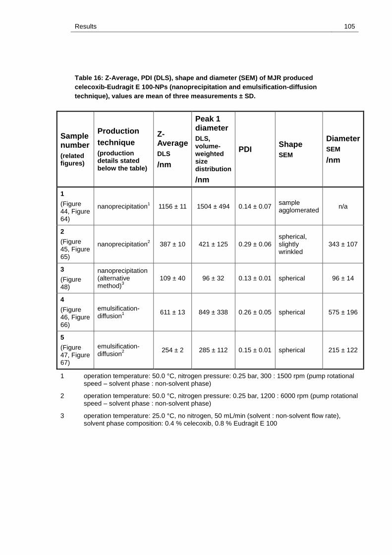
Results 105

Table 16: Z-Average, PDI (DLS), shape and diameter (SEM) of MJR produced

celecoxib-Eudragit E 100-NPs (nanoprecipitation and emulsification-diffusion

technique), values are mean of three measurements ± SD.

Sample number

(related figures)

Production

technique

(production details stated below the table)

Z-Average

DLS

/nm

Peak 1 diameter

DLS, volume-weighted size distribution

/nm

PDI Shape

SEM

Diameter

SEM

/nm

1

(Figure 44, Figure 64)

nanoprecipitation1 1156 ± 11 1504 ± 494 0.14 ± 0.07

sample agglomerated

n/a

2

(Figure 45, Figure 65)

nanoprecipitation2 387 ± 10 421 ± 125 0.29 ± 0.06

spherical, slightly wrinkled

343 ± 107

3

(Figure 48)

nanoprecipitation (alternative method)

3

109 ± 40 96 ± 32 0.13 ± 0.01 spherical 96 ± 14

4

(Figure 46, Figure 66)

emulsification-diffusion

1

611 ± 13 849 ± 338 0.26 ± 0.05 spherical 575 ± 196

5

(Figure 47, Figure 67)

emulsification-diffusion

2

254 ± 2 285 ± 112 0.15 ± 0.01 spherical 215 ± 122

1 operation temperature: 50.0 °C, nitrogen pressure: 0.25 bar, 300 : 1500 rpm (pump rotational speed – solvent phase : non-solvent phase)

2 operation temperature: 50.0 °C, nitrogen pressure: 0.25 bar, 1200 : 6000 rpm (pump rotational speed – solvent phase : non-solvent phase)

3 operation temperature: 25.0 °C, no nitrogen, 50 mL/min (solvent : non-solvent flow rate), solvent phase composition: 0.4 % celecoxib, 0.8 % Eudragit E 100

106 Results

Figure 44: SEM image (a) and volume-weighted DLS size distribution report (b) of MJR

produced celecoxib-Eudragit E 100-particles (nanoprecipitation technique): NP

properties (determined by DLS, mean of three measurements): 1156 nm (Z-Average),

0.144 (PDI).

Results 107

Figure 45: SEM image (a) and volume-weighted DLS size distribution report (b) of MJR

produced celecoxib-Eudragit E 100-NPs (nanoprecipitation technique): NP properties

(determined by DLS, mean of three measurements): 387 nm (Z-Average), 0.285 (PDI).

108 Results

Figure 46: SEM image (a) and volume-weighted DLS size distribution report (b) of MJR

produced celecoxib-Eudragit E 100-NPs (emulsification-diffusion technique): NP

properties (determined by DLS, mean of three measurements): 611 nm (Z-Average),

0.258 (PDI).

Results 109

Figure 47: SEM image (a) and volume-weighted DLS size distribution report (b) of MJR

produced celecoxib-Eudragit E 100-NPs (emulsification-diffusion technique): NP

properties (determined by DLS, mean of three measurements): 254 nm (Z-Average),

0.148 (PDI).

110 Results

Figure 48: SEM image (a) and volume-weighted DLS size distribution report (b) of MJR

produced celecoxib-Eudragit E 100-NPs (nanoprecipitation technique–alternative

method using HPLC pumps and a non-solvent phase without surfactant, see chapter

2.2.1.2): NP properties (determined by DLS, mean of three measurements): 109 nm (Z-

Average), 0.132 (PDI).

Results 111

3.2.4 Atomic force microscopy

Figure 49 shows AFM images (two different enlargements of the same

sample) of MJR produced celecoxib-Eudragit E 100-NPs. These NPs were

prepared by the alternative nanoprecipitation method (see chapter 2.2.1.2

usage of HPLC pumps instead of micro annular gear pumps and of water

without surfactant as non-solvent phase). The volume-weighted size

distribution report of these NPs is shown in Figure 48.

In these images length and width of the NPs can be derived from the axis

below and at the side of the images. The color scale between the images

indicates the height of the NPs ranging from white (≥ 150 nm) over yellow

(75 nm) to black (0 nm).

The NPs exhibited a narrow size-distribution with diameter values between

circa 50 to 100 nm. All particles were of spherical or almost spherical shape.

This correlates well with the SEM characterization of these NPs (see the third

sample in Table 16 and Figure 48).

112 Results

Fig

ure

49:

AF

M im

ag

es

(tw

o d

iffe

ren

t en

larg

em

en

ts o

f th

e s

am

e s

am

ple

) o

f M

JR

pro

du

ced

cele

co

xib

-Eu

dra

git

E 1

00-N

Ps

(nan

op

recip

itati

on

te

ch

niq

ue

–alt

ern

ati

ve

meth

od

usin

g H

PL

C p

um

ps a

nd

a n

on

-so

lven

t p

hase w

ith

ou

t su

rfacta

nt,

see c

hap

ter

2.2

.1.2

): N

P

pro

pert

ies (

dete

rmin

ed

by D

LS

, m

ean

of

thre

e m

ea

su

rem

en

ts):

109 n

m (

Z-A

vera

ge),

0.1

32 (

PD

I);

vo

lum

e-w

eig

hte

d D

LS

siz

e d

istr

ibu

tio

n

rep

ort

sh

ow

n in

Fig

ure

48

(b

).

Results 113

3.3 Dissolution testing

3.3.1 Evaluation of a suitable dissolution medium for the API release of

celecoxib-Eudragit E 100-NPs

3.3.1.1 Dissolution test in diluted HCl (pH 1.2)

All nanosuspensions, which were used for the dissolution tests in chapter

3.3.1, were prepared by the alternative MJR nanoprecipitation method

(without addition of a surfactant to the non-solvent phase, see

chapter 2.2.1.2). First, a dissolution test of MJR-produced celecoxib-

Eudragit E 100-NPs in diluted HCl (pH 1.2) was performed as described in

chapter 2.2.3.2 (experimental set-up depicted in Figure 25). In short, 1 mL of

the nanosuspension to be tested was added to a 150 mL beaker containing

99 mL of the dissolution medium. The medium was stirred, using the

magnetic stirrer (for details see Table 6), at 300 rpm, and maintained at

37 ± 0.5 °C using the temperature sensor and the heating plate of the

magnetic stirrer. The peristaltic pump with the attached tubes carried the

medium continuously through the CF module. Respectively 2 mL of filtrate,

containing the dissolved API/analyte, were withdrawn at the defined sampling

points and applied to UV-Vis analysis.

The results are shown in Figure 50 and Table 30. Hence, more than 50 %

drug release occurred within 9 min. Up to 12 min this value remained

constant followed by a successive decline of the concentration until 34 % at

60 min.

114 Results

Figure 50: Dissolution of celecoxib-Eudragit E 100-NPs in HCl pH 1.2: NP properties:

80 nm (Z-Average), 0.131 (PDI) and 2.573 mg/mL (celecoxib concentration of the

nanosuspension, i.e. a 2.573 mg dose of celecoxib), detection: UV-Vis (248 nm), n=3,

red lines represent SD.

For the purpose of a detailed investigation of the analyte concentration

decline, a SEM image of the same nanosuspension in HCl pH 1.2 was taken

(see Figure 51). Thereto, a 1:100 dilution of the nanosuspension in HCl

pH 1.2 (dilution factor corresponds to the dissolution experiment) was stored

for 24 h at ambient temperature in a closed container. This was done to

simulate the reaction of the NPs with the dissolution medium. Then, this

sample was prepared for the SEM analysis without further dilution or washing

as described in chapter 2.2.2.5.

Thereby, rectangular particles in a size range of a few microns appeared,

while no NPs were visible.

Results 115

Figure 51: SEM image with precipitations of a 1:100 dilution of celecoxib-

Eudragit E 100-NPs in 0.1 M HCl after 24 h storage at ambient temperature; NP

preparation parameters: MJR, nanoprecipitation technique-alternative method

(without usage of a surfactant).

116 Results

3.3.1.2 Dissolution test in diluted HCl (pH 1.2) containing NaCl

The second dissolution test was performed with HCl pH 1.2 containing

0.15 M NaCl to examine the influence of electrolyte addition. Hence, another

NP batch was used than in chapter 3.3.1.1, but the preparation method was

the same and Z-Average, PDI and API concentration are similar. The test

parameters were the same as in chapter 3.3.1.1. The dissolution profile is

shown in Figure 52 (values stated in Table 31) together with the profile

without NaCl (from Figure 50) for comparison.

Hence, the dissolution rate was, in the presence of NaCl, faster and

celecoxib was completely dissolved at 12 min. Thereafter, a concentration

decline again occurred up to a value corresponding to 54 % dissolution.

Figure 52: Dissolution of celecoxib-Eudragit E 100-NPs in HCl pH 1.2 + 0.15 M NaCl:

NP properties: 100 nm (Z-Average), 0.100 (PDI) and 2.331 mg/mL (celecoxib

concentration of the nanosuspension, i.e. a 2.331 mg dose of celecoxib), detection:

UV-Vis (248 nm), n=1.

Results 117

3.3.1.3 Dissolution tests in diluted HCl (pH 1.2) containing cetrimide

Albers et al. [5] used cetrimide to ascertain sink conditions for release testing

of celecoxib-Eudragit E-extrudates. Thus, the dissolution behavior of the NPs

was examined in HCl pH 1.2 including 0.001, 0.01, 0.3 and 1.0 % (see Figure

53 and Table 32). Hence, the nanosuspension and the test parameters were

the same as in chapter 3.3.1.1.

Hereby, the dissolution profile obtained with 0.001 % cetrimide resembled

that one of pure HCl pH 1.2 (see Figure 50) with the exception that both initial

increase and following decrease were more intensive. Using 0.01 %, a

maximum concentration of 34 % was reached at 21 min followed by slight

decrease up to 30 % at 120 min. In contrast to these profiles a concentration

decline did not occur if 0.3 % (sink conditions [2]) or 1.0 % of surfactant was

used, while the slope was higher for 0.3 % than for 1.0 % with maxima at

39 % and 25 % API dissolved, respectively.

118 Results

Figure 53: Dissolution of celecoxib-Eudragit E 100-NPs in HCl pH 1.2 +

0.001/0.01/0.3/1.0 % cetrimide: NP properties: 80 nm (Z-Average), 0.131 (PDI) and

2.573 mg/mL (celecoxib concentration of the nanosuspension, i.e. a 2.573 mg dose of

celecoxib), detection: UV-Vis (248 nm), n=1.

Results 119

3.3.1.4 Dissolution tests in diluted HCl (pH 1.2) containing cetrimide

using cross-flow- and dead-end filtration

With regard to the issue that the dissolution process, even under sink

conditions, was not completed after 120 min (see chapter 3.3.1.3) the effect

of filter type and filter pore size were investigated. Hence, a nanosuspension

was used with a Z-Average of 160 nm, a PDI of 0.094 and a celecoxib

concentration of 2.388 mg/mL (same preparation method as in chapter

3.3.1.1).

These dissolution tests were performed under sink conditions (HCl pH 1.2 +

0.3 % cetrimide) using three different filters: the 100 kDa CF module

(MWCO: 10 nm), which was already used in the previous dissolution tests,

and a 500 kDa CF module (MWCO: 50 nm) as well as 0.2 µm syringe filter

holders to represent dead-end filtration. The sample withdrawal with the

syringe filter holders was performed analogously to conventional dissolution

tests and is described in chapter 2.2.3.3. The applicability of the new module

to retain these NPs was proven with the same procedure, which is described

in chapter 2.2.3.1. In the same way the 0.2 µm syringe filter holders were

tested successfully. The volume-weighted DLS size distribution reports of the

verification of both filters are shown in the appendix (see Figure 68). Apart

from the different filtration types the dissolution tests were performed as

described in chapter 3.3.1.1

Figure 54 reveals a great difference between the dissolution profiles obtained

with, on one hand, the 500 kDa CF module and 0.2 µm syringe filter holders

and, on the other hand, the 100 kDa CF module (values stated in Table 33).

In the latter case the experimental values did not exceed 10 % of the

maximum amount after 120 min. Conversely, nearly 100 % dissolution were

reached after only 3 min with both the 500 kDa CF module and the 0.2 µm

syringe filter holder at slightly higher initial increase with the syringe filter

holder.

To investigate whether the NPs are dissolved, 1:100 dilutions of the tested

nanosuspension in both water and 0.1 M HCl + 0.3 % cetrimide were

prepared. These dilutions were respectively filled without filtration in a cuvette

of the DLS instrument and measured at 37 °C (dissolution test temperature).

120 Results

The sample in dissolution medium was measured at several timepoints from

0–15 min (incubation time in the cuvette at 37 °C). The measurement at

15 min and the comparison in water are shown in the appendix (see Figure

69). Hence, it was observed that the NPs were completely dissolved in the

dissolution medium.

Figure 54: Dissolution of celecoxib-Eudragit E 100-NPs in diluted HCl pH 1.2 + 0.3 %

cetrimide: NP properties: 160 nm (Z-Average), 0.094 (PDI) and 2.388 mg/mL (celecoxib

concentration of the nanosuspension, i.e. a 2.388 mg dose of celecoxib), filters: CF

modules of 100 kDa and 500 kDa and 0.2 µm syringe filter holders (dead-end),

detection: UV-Vis (248 nm), n=3, red lines represent SD.

To achieve a slower dissolution rate the cetrimide concentration in the

medium was decreased to 0.05 % (m/V) and the dissolution tests performed

as described above. Hence, if using the 100 kDa CF modules, the maximum

release increased, compared to the medium with 0.3 % cetrimide, from 9 %

to 14 % maximum release (see Figure 55 and

Results 121

Table 34). Concerning the 500 kDa CF module, a similar curve progression

as previously was obtained with the exception that the release after 120 min

did not exceed 89 %. This was similar if the 0.2 µm syringe filter holders were

used, while the related profile exhibited a slower increase between 3 min and

20 min (~72 % to 84 %). This indicates insufficient solubilization of celecoxib

(see chapter 4.2).

Figure 55: Dissolution of celecoxib-Eudragit E 100-NPs in diluted HCl pH 1.2 + 0.05 %

cetrimide: NP properties: 160 nm (Z-Average), 0.094 (PDI) and 2.509 mg/mL (celecoxib

concentration of the nanosuspension, i.e. a 2.509 mg dose of celecoxib), filters: cross-

flow filtration modules of 100 and 500 kDa and 0.2 µm syringe filter holders (dead-

end), detection: UV-Vis (248 nm), n=3, red lines represent SD.

122 Results

3.3.1.5 Dissolution tests in phosphate buffers of different pH containing

0.3 % cetrimide

As the usage of a strongly acidic medium (HCl pH 1.2) in combination with

0.3 % cetrimide led to immediate and nearly complete release of celecoxib

(see Figure 54), different phosphate buffers of higher pH values were tested

towards their suitability to generate a dissolution profile, which is more

suitable to compare differently-sized NP batches. Furthermore, a high degree

of dissolution should be achieved. Hence, a nanosuspension was used with a

Z-Average of 220 nm, a PDI of 0.086 and a celecoxib concentration of

3.666 mg/mL (same preparation method as in chapter 3.3.1.1). The test

parameters were the same as in chapter 3.3.1.1 except that a 500 kDa CF

module was used.

Hence, the respective values after 120 min dissolution increased from

32.4 ± 3.6 API release at pH 5.2 to 88.8 ± 1.2 API release at pH 2.0 (see

Figure 56 and Table 35). The slope of the dissolution curves from the first

sampling point at 3 min to 120 min became smaller with decreasing pH (~23–

31 % release at pH 5.2 versus ~81–89 % at pH 2.0).

Results 123

Figure 56: Dissolution of celecoxib-Eudragit E 100-NPs in phosphate buffer

pH 2.0/2.5/3.5/4.5/5.2+ 0.3 % cetrimide: NP properties: 220 nm (Z-Average), 0.086 (PDI)

and 3.666 mg/mL (celecoxib concentration of the nanosuspension, i.e. a 3.666 mg

dose of celecoxib), filter: 500 kDa cross-flow filtration module, detection: UV-Vis

(248 nm), n=3, red lines represent SD.

124 Results

3.3.2 Comparison of the dissolution behavior of nanoparticles of

different size and unprocessed celecoxib particles

Finally, the dissolution profiles of NPs of different size (220, 250, 300, 350

and 500 nm) and unprocessed celecoxib particles were compared in

phosphate buffer pH 2.0 + 0.3 % cetrimide as medium to achieve a high

degree of dissolution (see chapter 3.3.1.5). The size of the unprocessed

particles was determined by laser light diffraction (volume-weighted median

diameter: 22.58 µm, size distribution report shown in the appendix Figure

70). Thereto, API powder was suspended in water and the suspension

simultaneously ultrasonicated and stirred before it was measured. The NPs

of different size were prepared by MJR technology as described in chapter

3.1.2.1 (emulsification-diffusion, with usage of Poloxamer 407 in the non-

solvent phase). The test parameters were the same as in chapter 3.3.1.1

except that a 500 kDa CF module was used and that 0.25 mL of each

nanosuspension were used for each dissolution test.

Hence, the profiles obtained for nanosuspensions strongly resemble each

other (see Figure 57). From start to 20 s they moderately increased up to

circa 10 % release, followed by sharp increase between 20 and 40 s to

approximately 80 % release. After 60 s circa 85 % of API were released.

From 60 s to the end of the test at 120 s there was no distinct change. In

contrast, the API powder samples showed nearly no release below 20 s.

Only from this timepoint on there was an increase to approximately 60 %

release at 120 s, while the slope of the curves slightly decreased up to this

point (see Figure 57). After 60 min 84.5 ± 12.6 % of API powder was

dissolved (see Table 36).

The statistical evaluation (for description see chapter 2.2.3.6), results stated

in Table 17) did not reveal significant changes between any of the

nanosuspension dissolution profiles with f1 values below 15 and f2 values

from 50–100 for every comparison. Though, the dissolution behavior of the

unprocessed API particles was clearly distinguished from all

nanosuspensions (f1 > 15 and f2 < 50).

Results 125

Figure 57: Dissolution of celecoxib-Eudragit E 100-NPs of different size and celecoxib

(API) powder in phosphate buffer pH 2.0 + 0.3 % cetrimide: NP properties:

221/255/293/362/497 nm (Z-Average), < 0.25 (PDI) and ~ 2.650–4.850 mg/mL (celecoxib

concentration of the nanosuspension, i.e. 0.663 mg-1.213 mg celecoxib dose), API

powder: 2537 µg/mL (celecoxib concentration of the suspension), filter: 500 kDa

cross-flow filtration module, detection: UV-Vis (248 nm), n=6, red lines represent SD.

126 Results

Table 17: Statistical comparison of dissolution profiles of celecoxib-Eudragit E 100-

NPs of different size and celecoxib (API) powder: Evaluation performed with model

independent approach using a similarity factor according to FDA “Guidance for

Industry: Dissolution Testing of Immediate Release Solid Oral Dosage Forms” [153],

equivalence is given if f1 < 15 (0–15) and f2 > 50 (50–100).

Comparison Difference

factor f1

similarity factor f2

Equivalence of dissolution curves

221 nm - 255 nm 5.3 74.5 yes

221 nm - 293 nm 3.8 77.7 yes

221 nm - 362 nm 4.0 75.7 yes

221 nm - 497 nm 3.6 81.9 yes

221 nm - API powder 61.6 26.9 no

255 nm - 293 nm 2.8 81.2 yes

255 nm - 362 nm 1.6 89.6 yes

255 nm - 497 nm 3.3 76.3 yes

255 nm - API powder 61.8 26.1 no

293 nm - 362 nm 1.6 99.2 yes

293 nm - 497 nm 1.7 98.1 yes

293 nm - API powder 62.5 26.8 no

362 nm - 497 nm 3.3 84.9 yes

362 nm - API powder 61.8 26.5 no

497 nm - API powder 61.8 27.2 no

Results 127

Since the performed evaluation did not reveal differences between the

dissolution behavior of the differently-sized NPs a second evaluation was

done. To detect the respective endpoints of dissolution the reciprocals of the

release percentages were plotted against the reciprocals of dissolution time.

Then, the y-intercept of the line through the last three sampling points was

determined (1/y-intercept = maximum release Rmax). The Rmax-values are

given in Table 18 and the graph for the NPs of ~350 nm diameter is

exemplarily shown below (see Figure 58).

In the next step the natural logarithm of the release was plotted against the

dissolution time. Hence, the release was corrected through division of the

respective values by the above-obtained Rmax-values. The dissolution time

was corrected by subtraction of the dead time td (~13 s, determined

experimentally, see chapter 2.2.3.4). To compare the dissolution velocities

the value k was determined as slope of the regression line through the first

three sampling points. The k-values are given in Table 18 and the graph for

the NPs of ~350 nm diameter is exemplarily shown below (see Figure 59).

Concerning the determined k-values there is a great difference between the

API powder (k = 0.017) and the NPs. Additionally the k-values of the NP

batches of 220 nm (0.124), 250 nm (0.138) and 500 nm (0.117) differ from

those of 300 nm (0.059) and 350 nm (0.087).

128 Results

Table 18: Rmax- and k-values of the dissolution of the differently-sized NP batches.

Rmax values obtained as y-intercept of a line through the last three sampling points

after plotting of the reciprocal of release percentage against the reciprocal of

dissolution time. k-values obtained as slope of the regression line through the first

three sampling points after plotting of the natural logarithm of release against

dissolution time.

Particle size /nm Rmax k

221 85.5 ± 0.6 0.124 ± 0.041

255 85.4 ± 0.5 0.138 ± 0.01

293 96.0 ± 1.8 0.059 ± 0.01

362 93.6 ± 0.1 0.087 ± 0.024

497 83.8 ± 1.4 0.117 ± 0.006

22580 (API powder)

84.5 ± 0.5 0.017 ± 0

Results 129

Figure 58: Plot of the reciprocal of release percentage against the reciprocal of

dissolution time for the NP batch of 362 nm diameter. The Rmax corresponds to the

reciprocal of the y-intercept of the red line through the last three sampling points.

130 Results

Figure 59: Plot of the natural logarithm of release against dissolution time for the NP

batch of 362 nm diameter (vertical bars represent the standard deviation). The k-value

corresponds to the slope of the red regression line through the first three sampling

points.

Discussion 131

4 Discussion

4.1 Nanoparticle preparation

The usage of the MJR technology for the production of NPs was based on

the doctoral thesis of Akif Emre Türeli [13]. Türeli prepared different NP

formulations using hydroxypropyl methyl cellulose phthalate (HPMCP 50),

low molecular weight chitosan and Eudragit S 100 as polymers. Fenofibrate,

Danazol and Gliclazide served as APIs. These formulations were gastro-

resistant. Additionally, he adapted the MJR technology (Penth, 2005 [11]) to

enable the custom preparation of NPs (see also 1.3.2). In the present study,

NPs were manufactured that can dissolve in the stomach by using Eudragit E

instead of Eudragit S. The API Celecoxib does not require a gastro-resistant

formulation, as it is an NSAR without harmful effect on the gastric mucosa

(see 1.2). Hence, the focus is on fast dissolution of the poorly-soluble API.

The most significant difference of the present study to the thesis of Türeli is

the development of a new and robust approach for dissolution testing of

nanoparticulate dosage forms. Türeli used the conventional USP 2 apparatus

with standard syringe filter holders to perform dissolution studies. The

disadvantages of this technique were intensively discussed above (see

chapters 1.5.2 and 1.5.3). Thereto, the prepared Celecoxib-Eudragit E-NPs

served as a model.

The combination of celecoxib and Eudragit E proved to be suitable to

produce extrudates by hot-melt extrusion [1][5]. After the extrusion the molten

mass was cooled and milled to obtain powders in different size fractions up to

500 µm. This process is a top-down approach (see chapter 1.3.1.1). In the

present study NPs of celecoxib and Eudragit E 100 were produced by a

bottom-up approach (see chapter 1.3.1.2) either as bench-top method or by

MJR technology. This study revealed that the bench-top preparation of

celecoxib-Eudragit E 100-NPs with emulsification-diffusion technique

requires an adequate co-stabilizer. Thereto, the applicability of three

stabilizers, two steric (PVA and Poloxamer 407) and one negatively charged

electrostatic stabilizer (SDS), for the NP production was tested (see

132 Discussion

chapter 3.1.1.1). Since the system already contained a positively charged

stabilizer (Eudragit E 100), the implementation of a further one was

considered to be ineffective due to repulsion between them.

Of this choice only Poloxamer 407 was appropriate. Concerning SDS,

aggregation with Eudragit E 100 molecules due to ionic interactions may

reduce surface charge and therefore stability. In case of PVA, the

arrangement with Eudragit E 100 molecules on the NP surface is obviously

unfavourable leading to relatively low ZP values (see Table 21) and likewise

poor stability. In contrast, the use of Poloxamer 407 resulted in significantly

higher ZP values (above 40 mV). Accordingly, every PDI value did not

exceed 0.25 while all values were higher for PVA stabilization. In summary,

every approach with Poloxamer 407 met the desired criteria of a Z-Average

between 100 and 500 nm, a PDI not more than 0.25 and a ZP of at least

20 mV while this did not apply for the most approaches with PVA or SDS.

Since Poloxamer molecules both include hydrophilic and hydrophobic

segments this effectively prevents aggregation due to steric hindrance [132].

Regarding the solvent : non-solvent ratio, only Poloxamer 407 at 1 : 5 and

1 : 10 ratios did not cause visible agglomeration after 24 h. A possible

explanation for the instability of the 1 : 2 ratio may be that celecoxib and

Eudragit E 100 precipitation continued after preparation due to delayed

evaporation of remaining ethyl acetate. Without agitation this can provoke

coalescence of solvent droplets leading to formation of larger particles and

finally agglomeration [21]. From current literature concerning preparation of

polymeric NPs, with both emulsification-diffusion and nanoprecipitation

technique, it is known that the use of higher concentrations of API/polymer in

smaller amounts of organic solvent is more common than vice versa and that

the preparation of suitable nanosuspensions generally requires a high degree

of supersaturation [28].

The smallest particles were obtained if using a 1 : 5 solvent : non-solvent

ratio (see Table 19). A possible explanation is that lower amounts of organic

solvent result in precipitation of API and polymer immediately after mixing. If

this occurs before the formation of a homogeneous nanoemulsion, the NP

size can be influenced since deposition on already existing nuclei is

Discussion 133

thermodynamically favoured [90]. Further explanations deliver the findings

from Deng et al. who prepared paclitaxel nanocrystals stabilized by

Poloxamer 407 [30]. They found that, at higher concentration, Poloxamer 407

can form micelles which pull Poloxamer molecules off the NP surface and

therefore lead to reduced stability and larger size. Due to the low particle

size, an adequate PDI and the relatively higher API content, the 1 : 5

solvent : non-solvent ratio was used in further experiments.

Concerning the Eudragit E 100 concentration, the use of 10 instead of

5 mg/mL in the solvent phase increased the NP size (about 50 nm for the

1 : 5 solvent : non-solvent ratio) at constant PDI. Though, the EE values were

consistently higher, which, according to literature, can be explained by an

increase in organic phase viscosity due to higher polymer content. Higher

viscosity might, in turn, reduce drug partitioning to the aqueous phase [39]. In

consideration of the molar masses of celecoxib (≈380 Da) and Eudragit E

monomers (≈400 Da) the higher Eudragit E : celecoxib ratio leads to a molar

excess of Eudragit E. This enables the complete molecular complexation of

celecoxib with Eudragit E (see Figure 60). Thus, it was given preference to a

Eudragit E 100 concentration of 10 mg/mL in the solvent phase.

Type and concentration of stabilizers are known to play an essential role to

inhibit crystal growth, which would cause instability of nanosuspensions [56].

Electrostatic stabilization depends on an interaction between repulsive

electrostatic forces and attractive van-der-Waals forces, the so-called DLVO

forces [31,158]. The charge on the particle surface provokes the formation of

an electrostatic double-layer in the direct environment of the particles, which

results in the zeta potential (see chapter 1.4.2). Ideally, a sufficiently high ZP

avoids approximation of the particles and prevents agglomeration. The use of

ionic surfactants and polymers is regarded to be the most effective way to

stabilize NP dispersions [151].

Since the system of combined stabilization (Eudragit E 100 and

Poloxamer 407) proved to be suitable for the production of celecoxib NPs,

the influence of the stabilizer concentration was examined in the next step

(see chapter 3.1.1.2). It is in good agreement with literature data that the NP

diameter tends to decrease with increasing Poloxamer concentration (see

134 Discussion

Figure 28 (a)) [64]. Higher concentrations of stabilizer molecules will more

effectively protect the creating nuclei from agglomeration. This likewise

explains the decrease of the PDI, i.e. the higher homogeneity of the NPs.

However, an increase from 2.5 mg/mL to higher concentrations of

Poloxamer 407 did not lead to further improvement of PDI or decline of size.

Additionally, at these concentrations the ZP values were lower. Thus, it can

be assumed that an optimal arrangement of Eudragit E 100 and

Poloxamer 407 molecules on the NP surface is achieved between 1 and

2.5 mg/mL Poloxamer 407 concentration in the non-solvent phase leading to

the lowest size at adequate PDI and ZP.

Figure 60 (a) depicts a schematic of the NPs according to the assumed

model. Hence, the NP surface is positively charged due to the tertiary amino

groups of Eudragit E 100, which are protonated at neutral or acidic pH [82].

Dissolved Poloxamer 407 molecules act as steric stabilizer. The combination

of non-ionic with ionic stabilizers is regarded to be more effective than ionic

or non-ionic stabilization alone. This is due to inclusion of non-ionic between

ionic stabilizer molecules, which reduces self-repulsion and therefore

facilitates a more suitable arrangement on the NP surface [164]. Celecoxib

molecules form complexes (ionic interaction) with Eudragit E molecules. This

is facilitated by the protonated tertiary amino groups of Eudragit E and the

deprotonated sulfone amide groups of celecoxib (Figure 60 (b), chemical

equation shown in Figure 61). Figure 60 (c) shows the aromatic (celecoxib)

and aliphatic (Eudragit E and Poloxamer 407) hydrophobic domains of the

molecules. Hence, hydrophobic interactions are possible between all

involved molecules. These interactions are much weaker than electrostatic

interactions [8]. In case of the bonding between Eudragit E and

Poloxamer 407 it is the sole interaction. In-vivo the hydrophobic domain and

the rigid ring structure of celecoxib advise an interaction with bile salts

(solubilization in the duodenum) [10]. Further results (DSC and IR, see

chapters 3.2.1 and 3.2.2 and discussion below) reinforce this model in case

of the NPs prepared with emulsification-diffusion technique. However, these

methods indicate different chemical interactions in the NPs, which were

prepared using the nanoprecipitation technique.

Discussion 135

Figure 60: (a) Schematic of a celecoxib-Eudragit E 100-NP in aqueous suspension co-

stabilized by Poloxamer 407: Celecoxib (white spheres) molecular complexes

embedded in a matrix of Eudragit E 100 (orange sphere). Surface charge is positive

due to protonated Eudragit molecules (orange lines). Poloxamer 407 (blue lines)

molecules contribute to stabilization by inclusion between Eudragit molecules. (b)

Molecular complex of celecoxib and Eudragit E 100, dotted line shows ionic

interaction. (c) Hydrophobic domains (dotted circles) of Eudragit, Poloxamer and

celecoxib molecules.

The EE values (see Figure 28 (b)) decreased over the examined range with

increasing Poloxamer 407 concentration. These results show that higher

Poloxamer concentrations are accompanied by higher celecoxib

concentrations in the supernatant. With regard to the surface-active

properties of Poloxamer this is very probably due to enhanced solubilization

of celecoxib. Finally, a 2.5 mg/mL Poloxamer 407 concentration in the non-

solvent phase is regarded to be optimal. Beyond this point the size and the

PDI could not be improved by increasing the concentration, while the EE

decreased.

136 Discussion

The lowest therapeutic single dose of celecoxib is 50 mg [47]. An EE of 70 %

provided (value of the optimized formulation, see above), circa 70 mL of the

nanosuspension would be necessary to administer this amount. Thereto,

NPs with higher celecoxib and Eudragit E 100 concentrations were prepared

(see chapter 3.1.1.3). For each nanosuspension was the absolute value of

the ZP sufficiently high (> 30 mV) to ascertain adequate stabilization.

According to literature, a ZP value of at least ± 20 mV is convenient, provided

that the system is, in combination, electrostatically and sterically stabilized

[164].

Though, the pre-defined criteria concerning size and homogeneity

(Z-Average < 500 nm and PDI < 0.25) were not met if using a celecoxib

concentration in the solvent phase of 50 mg/mL or more. At higher

concentrations the stabilizers were obviously not able to protect the NPs from

agglomeration, why these nanosuspensions are inappropriate despite the

high EE values. In conclusion, the formulations prepared with 25 mg/mL

celecoxib and 50 mg/mL Eudragit E 100 in the solvent phase and

12.5 mg/mL Poloxamer 407 in the non-solvent phase were not equivalent to

those prepared with 5 mg/mL celecoxib and 10 mg/mL Eudragit E 100.

However, they still fulfil the required criteria regarding size and homogeneity

to a particularly high degree (Z-Average ~350 nm versus 200 nm, ZP of ~36

versus 39 mV and PDI ~0.1 versus 0.05) and provide higher EE (85 %

versus 72 %).

In a stability study two formulations, one prepared with 5 mg/mL, the other

with 25 mg/mL celecoxib in solvent phase, were compared if stored at 5 °C

and room temperature, respectively (see chapter 0). In this context, it

emerged that the formulation with the higher celecoxib content was superior

if it was stored at room temperature. First, both Z-Average and PDI remained

constant over a period of 14 d (see Figure 32) while the other samples under

test became inhomogeneous after three or four days storage. Analogously,

the ZP values changed (see Figure 33). The EE was significantly higher over

the complete storage period if more celecoxib and Eudragit E 100 were used

independent on the storage temperature (see Figure 34).

Discussion 137

Hence, it is to consider that the use of higher API and excipient

concentrations in the solvent phase provokes a more intense supersaturation

after contact with the non-solvent phase, which is only partially compensated

by the use of more surfactant. First of all, this explains the higher EE values

obtained at the higher concentration, i.e. higher amounts of celecoxib and

Eudragit E 100 precipitate as NPs and smaller amounts are dissolved in the

surrounding liquid (determined as concentration in the supernatant). This has

two consequences: First, it is desirable to achieve high EE values to increase

the yield of nanoparticulate API. Second, higher concentrations of dissolved

API/excipient are accompanied by higher probability of delayed and therefore

uncontrolled precipitation.

Concerning the storage conditions room temperature was more

advantageous than 5 °C. While there was no significant change in the

Z-Average over the complete period the PDI values of the approaches stored

at 5 °C increased after day three compared to room temperature. This may

be caused by crystallization, which, as an exothermic process, is enhanced

at lower temperatures. After 28 d at every sample sharp needles appeared

on the interior wall of the container, while the liquid was clear. This was

attributed to crystallization. The storage temperature had no apparent

influence on ZP and EE.

Since, as mentioned above, the highest possible API concentration is

preferred and due to better stability, was the optimization of the NP

preparation with MJR technology based on the higher-concentrated

composition of API and excipients. Thereby, implementing DoE, NPs in size

range from 300 to 450 nm of narrow size distribution (PDI < 0.25) could be

produced. The ZP and EE values were very similar to those obtained from

NPs prepared with the BT procedure. The DoE equation (20), which

implements three MJR variables (temperature, nitrogen pressure and flow

rate), provided a good correlation. The calibration function (see Figure 37),

which was obtained by comparing the measured Z-Average values of certain

NP preparations to the corresponding predicted values, likewise has a good

correlation of approximately 0.88. Additionally, there was no obvious trend

concerning deviation of the single values. Thus, the developed model proved

138 Discussion

to be appropriate for the fast and controlled manufacture of celecoxib NPs in

different size ranges.

As an alternative to emulsification-diffusion technique, NPs were prepared by

the nanoprecipitation technique. However, these NPs were not equivalent to

those prepared by emulsification-diffusion. First, their size distribution was

broader being demonstrated by higher PDI values, which failed to meet the

criterion to be lower than 0.25. Additionally, lower ZP values (~ 35 mV versus

~ 45 mV) indicated worse stability. Concerning the EE, equivalent values

were obtained if using a pump rotational speed of 300 : 1500 rpm

(solvent : non-solvent), while a 1200 : 6000 rpm ratio mainly led to

significantly lower values. Thus, this setting was obviously inappropriate to

generate adequate mixing conditions in the reactor chamber. Additionally,

NPs were produced by the nanoprecipitation technique with an alternative

method (see chapter 2.2.1.2). Hence, the non-solvent phase was water

without addition of a surfactant and HPLC pumps with lower flow rates were

used. With this setup NPs of diameters from approximately 80–200 nm

(Z-Average), PDI values below 0.15 and ZP values from circa 40–60 mV

were obtained (see chapter 3.3.1 and Figure 68 (a)). These NPs had a

spherical shape, which was shown by SEM (see Figure 48) and AFM (see

Figure 49). The related nanosuspensions were stable over at least one

month. However, this method did not allow a reproducible production of NPs

of different sizes.

In general, it is to consider that, concerning a comparison between

nanoprecipitation and emulsification-diffusion method, a reliable statement

cannot be made since a full experimental design was not performed.

However, it can be concluded that nanoprecipitation is a suitable alternative

for preparation of celecoxib-Eudragit E 100-NPs but the controlled

manufacture of different sizes would require further experiments.

The obtained DSC curves (see chapter 3.2.1) provide an insight into the

thermal behavior of the NP components. Furthermore, they reveal

differences between the NPs and the blend of their components. Celecoxib is

a crystalline substance with a defined melting point Tm. From Figure 40 this

Discussion 139

value was determined to 164 °C as minimum of the endothermic peak, which

correlates well with the literature value of 162 °C [5]).

As a polymeric substance Eudragit E has no crystalline structure and,

therefore, a glass transition range instead of a defined melting point. From

the Eudragit E DSC trace the glass transition temperature Tg was determined

to 45 °C. This is likewise in good agreement with the literature value of 48 °C

[136]. The endothermic peak, which follows the glass transition range, may

be due to enthalpy relaxation. This is a typical phenomenon, which arises

from the fact that amorphous substances change their structure time-

dependent if they are stored below Tg to attain a thermodynamic equilibrium

[113]. The respective sample was manufactured approximately three years

before measurement.

In the curve of the physical mixture with Eudragit E 100 Tg was shifted to a

slightly lower value (42 °C). It is known that drug molecules can impede

intermolecular interactions leading to lower Tg, if they are located between

polymer chains, [5]. The melting peak of celecoxib was significantly

broadened indicating the presence of amorphous celecoxib, i.e. a solid

dispersion [27,137].

While this peak was further broadened and appeared at lower temperature in

case of the NPs prepared by nanoprecipitation it disappeared at NPs

prepared by emulsification-diffusion. This indicates that, in first case, a solid

dispersion with crystalline portion of celecoxib was formed while, in the

second case, celecoxib mainly exists in amorphous form.

In combination with the fact that Tg of Eudragit E was circa 8 °C lower, these

findings clearly indicate that, in both cases, the API molecules are embedded

in a matrix of the excipient as postulated above (see Figure 60). Furthermore,

the possibility to produce solid dispersions of celecoxib in Eudragit E has

already been shown [5].

Concerning the IR measurements (see chapter 3.2.2) it can first be stated

that ionization of celecoxib and Eudragit E 100 led to substantial changes in

the spectra. At celecoxib sodium the sulfone amide is deprotonated, which is

clearly recognizable from the missing SO2 and NH signals. Additionally, the

140 Discussion

CF3 bands were missing and out-of-plane vibrations were significantly

reduced. This may be attributed to distribution of the free electron over the

π-system of the molecule.

If the tertiary amino function of Eudragit E 100 was protonated, the doublet

signals being related to nitrogen bonds (N–CH3 and C–H vibrations)

coalesced. Contrary to celecoxib the molecule provides no mesomeric

system and further substantial changes, especially regarding the carbonyl

and ester signals, were missing.

Concerning the NP samples it was evident that those prepared with ethyl

acetate (emulsification-diffusion technique) were very similar to the blend of

the charged compounds while the opposite was the case for those prepared

with methanol (nanoprecipitation technique). In addition to the obtained DSC

results (see above) this confirms the assumption that NPs produced by

emulsification-diffusion are entirely amorphous while the others are partially

crystalline. This can possibly be explained by polarity differences between

the two solvents. Methanol, as a protic solvent, can be a competitor to the

very weak acid celecoxib as a proton donor. Consequently, less celecoxib

would be ionized, which is prerequisite for dissolution in the Eudragit E 100

matrix. In contrast, ethyl acetate, as an aprotic solvent, has no influence on

the acid-base reaction between celecoxib and Eudragit E 100.

Finally, SEM imaging revealed that most of the produced NPs were of

spherical shape (see chapters 3.2.3 and 3.2.4). This is advantageous since

the dissolution rate of spherical particles is increased towards equal-sized

particles of irregular shape [94]. Furthermore, they have in solid form more

favourable flow properties due to the relatively lower surface area and

consequently lower cohesive forces between the particles. This, in turn,

ensures more uniform packing and, therefore, increased dose uniformity [62].

Slight deviations from spherical shape appeared at NPs, which were

prepared by nanoprecipitation. This is in agreement with the findings

obtained from DSC and IR, which indicated a partially crystalline structure of

these NPs. Furthermore, size and uniformity of spherical NPs can reliably be

determined by non-imaging techniques like DLS [12]. This was corroborated

Discussion 141

by a good correlation between the NP diameters, which were determined

with DLS and SEM (see Table 16).

142 Discussion

4.2 Dissolution testing

The FDA database of dissolution methods [154] recommends two types of

media for the dissolution test of celecoxib capsules. The first is 1000 mL of a

0.04 M tribasic sodium phosphate buffer (pH 12) containing 1 % SDS as a

tier 1 medium. Alternatively, a tier 2 medium can be used. Thereto, the

dissolution test is started in 750 mL of simulated gastric fluid (USP) including

pepsin. After 20 min 180 mL of a SDS solution is added to reach a final

concentration of 1 % SDS, followed by circa 70 mL of 1.2 M NaOH to adjust

the pH to 12. The sampling points are at 10, 20, 30, 45 and 60 min. The

selection of these media relies on the fact that celecoxib is, as a weak acid,

soluble in strong alkalis and that the usage of surfactants can enhance the

solubility.

However, a basic or neutral medium is not applicable for the dissolution of

celecoxib-Eudragit E 100-NPs since Eudragit E is intended to be dissolved in

gastric fluid up to pH 5.0 [40]. Dissolution media of basic or neutral pH would

inhibit the disintegration of the Eudragit E 100 matrix and, consequently, the

release of celecoxib. Thus, the dissolution behavior in diluted HCl without any

surfactant was examined first. As the stomach is the intended dissolution site

for the NPs in-vivo, the pH was adjusted to 1.2. This value is recommended

by the FDA to simulate gastric fluid [153].

The dissolution profile obtained with this medium showed an uncommon

course (see Figure 50). Usually the API concentration reaches a maximum at

a certain timepoint that either corresponds to 100 % dissolution or the

saturation solubility of the analyte. Then, this value remains constant until the

end of the test. A curve progression showing a maximum followed by a

decline indicates that dissolved API precipitates after a certain time span.

This circumstance was confirmed by taking a SEM image of the same

nanosuspension after 24 h incubation in HCl pH 1.2. Thereby, microparticles

of non-spherical shape appeared. The same observation has been made by

Albers et al. [2].

These findings can be explained if considering the specific structure of the

NPs (see Figure 60). Since the API (celecoxib) is embedded in a matrix of

Discussion 143

the excipient (Eudragit E 100) the presence of a so-called solid dispersion

can be presumed. A plethora of publications exists in this field while Craig

(2002) [27] has reviewed the release mechanisms of drugs out of solid

dispersions in detail. Hence, there exist two mechanisms: carrier-controlled

and drug-controlled dissolution. Both mechanisms implement a layer around

the particles that is rich of dissolved polymer (matrix material) and has to be

passed by the drug. How this occurs in detail depends on the viscosity of the

polymer-rich layer which itself is controlled by the polymer concentration. At

carrier-controlled dissolution the time for the particles to be released into the

medium is insufficient. Therefore, dissolution of the drug in the polymer-rich

layer is provoked. Here, diffusion through this layer is the rate-determining

step and can be described by the Stokes-Einstein equation (5). In contrast, at

drug-controlled dissolution, the drug particles dissolve comparatively slow in

the polymer layer and reach the medium mainly intact. In this case, the

dissolution process is determined by the physicochemical properties of the

drug like, for instance, the particle size.

Which of these mechanisms dominates in the present system cannot be

postulated with utmost certainty. Dubois and Ford (1985) [35] examined the

dissolution rates of ten drugs as solid dispersions in PEG 6000 using the

rotating disc methodology. Their results indicate that carrier-controlled

dissolution might only occur up to a certain drug-polymer ratio. On this basis

one may assume that drug-controlled dissolution is the favored mechanism in

the present system. However, as even the initial particle size is in nanometer

range, this is not necessarily an obstacle for fast and effective release of the

API.

Albers et al. (2009) [5] produced different hot-melt extrudates, also consisting

of celecoxib and a polymethacrylate carrier. They, inter alia, performed

dissolution experiments in 0.1 M HCl and measured for one formulation after

5 min an API release being 58-fold higher than the saturation solubility at this

pH. Though, they observed thereafter a distinct decline within a few minutes.

This resembles the obtained results (see Figure 50) and can be explained by

the fact that the solubility of amorphous substances is higher than that of the

corresponding crystalline form due to their lower thermodynamic stability.

144 Discussion

However, when the amorphous drug gets into contact with the dissolution

medium two processes start: on one hand the dissolution, but on the other

hand crystallization of the API as this is the thermodynamically preferred

form. Therefore, recrystallization of dissolved API can lead to a decline of the

measured concentration [5].

Since 100 % dissolution was not obtained if using diluted HCl the next issue

was to achieve complete dissolution of celecoxib and to inhibit

recrystallization. Therefore, it is commonly recommended to provide sink

conditions [153]. In USP chapter <1092> sink conditions are defined as “the

volume of medium at least three times that required in order to form a

saturated solution of drug substance” [150]. The used nanosuspension

volume for the previous dissolution tests contained a celecoxib amount of

nearly ten-fold above the saturation solubility at pH 1 (3.15 mg/L) [4].

In general, there are two approaches to counter this issue: first, one can

increase the volume of dissolution medium to a level that grants sink

conditions. However, it is to consider that API amounts used for dissolution

tests should reflect a single therapeutic dose. Consequently this would

necessitate a medium volume of at least 17 L which is hardly feasible in

practice. The second approach is to add substances being able to enhance

the API solubility which would allow keeping the medium volume lower.

Different research groups have shown that electrolytes can improve

dissolution of complexes consisting of Eudragit E and anionic drugs [77,120].

Quinteros et al. (2008) [120] titrated several such complexes with a NaCl

solution and plotted the pH value against the time. They mainly attributed the

occurring pH shift to an exchange of the deprotonated acid, i.e. the API, by a

chloride ion. Then, the acid withdraws the proton from Eudragit leading to an

increase in pH. Taking the example of a system of celecoxib and Eudragit E

this process is described in the chemical equations below (see Figure 61).

Since both the chloride of Eudragit E and the sodium salt of celecoxib are

well water-soluble this is favorable for dissolution.

Discussion 145

[Cel−

EUH+] + NaCl ⇌ [EUH

+Cl

−] + Cel−

+ Na+ (a)

Cel−

+ H+⇌ CelH (b)

Figure 61: Equations of the reaction of celecoxib-Eudragit E complex with NaCl

leading to exchange of deprotonated celecoxib by a chloride ion (a) followed by

protonation of celecoxib (b) (Cel = celecoxib and EU = Eudragit E).

Kindermann et al. (2011) [77] performed dissolution studies of hot-melt

extruded complexes of naproxen and Eudragit E. As dissolution medium they

added different electrolytes in various concentrations to a 0.001 % aqueous

solution of polysorbate 20. After electrolyte addition the dissolution rate

increased depending on type and concentration of the electrolyte, while a

0.15 M NaCl solution was found to be most suitable.

The addition of NaCl in this concentration to the medium was proven to be

beneficial for both rate and degree of dissolution. Though, even if 100 %

dissolution were obtained, this value could not be maintained and a

concentration decline occurred, which was even more intense than with

diluted HCl alone (see Figure 52). Here, it must be kept in mind that the

concentration of dissolved API is at maximum about ten-fold higher than its

saturation solubility. In summary, this means that electrolyte addition can be

used to increase the dissolution rate of polyelectrolyte complexes but is not

appropriate to improve the solubility. This meets the results obtained from

Kindermann et al. who observed that the dissolution process of naproxen,

even in presence of electrolytes, stopped in its saturation solubility [77].

Since electrolyte addition to the medium was not sufficient to achieve a

satisfactory dissolution profile it was necessary to search for an appropriate

alternative. In pharmaceutical dissolution testing, surfactants are extensively

used to improve dissolution profiles of sparingly water-soluble APIs

[12,139,153]. Bates et al. discussed in 1966 that addition of surfactants to the

dissolution medium enhances the saturation solubility and, therefore, the

dissolution rate [12]. This is due to the fact that this rate, according to the

Noyes-Whitney equation (15), linearly depends on the saturation solubility.

This effect is caused by two mechanisms: first, surfactants decrease the

146 Discussion

interfacial tension between API and dissolution medium, second, the API can

be solubilized within micelles. Naturally, the latter mechanism is only relevant

if surfactants are used in a concentration above the CMC, i.e. the point from

which micelles are formed to a significant extent. If solubilization in micelles

occurs, Bates et al. consider this to play the major role [12].

The compendial dissolution method for Celebrex© capsules involves the

usage of 1 % SDS [154], which is a wide-spread and well-suitable additive to

dissolution media [139]. However, this surfactant may not be suitable for drug

release out of a Eudragit E matrix as cationic Eudragit E could possibly

interact with anionic SDS. Thus, a cationic or non-ionic surfactant would be

recommendable. Since Albers et al. (see above) performed dissolution

studies of extrudates also consisting of celecoxib and Eudragit E, it was

decided to utilize cetrimide (see Figure 62). This is a cationic surfactant

which was added to 0.1 M HCl to ascertain sink conditions (solubility of

celecoxib in HCl pH 1.2 + 0.3 % cetrimide: 254.19 mg/L) [5].

Figure 62: Structure of cetrimide.

First, the use of cetrimide did, regardless of the concentration, not have the

expected effect of fast and complete dissolution of the API. If cetrimide

concentration was in a range, which cannot provide sink conditions, a decline

after a certain time occurred as already observed (see Figure 50 and Figure

53). This decline did not appear at higher concentrations of cetrimide where

sink conditions are given. This can be explained by the fact, that solubility

enhancement due to nanoscaling may not be sufficient to have a decisive

influence on saturation solubility in the present case. However, it is

contradictory that the dissolution rate decreases with increasing surfactant

concentration. This can possibly be explained if considering the mechanisms

of solubility and dissolution rate enhancement of surfactants (see above).

Hence, Bates et al. consider solubilization within micelles to be of essential

importance besides the reduction of interfacial tension [12].

Discussion 147

At 30 °C cetrimide forms micelles with an aggregation number of 75-120 [19].

Shanthi et al. determined the CMC of cetrimide in water to 3.88 mM at

ambient temperature [140], which corresponds to a concentration of

1.4 mg/mL respectively 0.14 % (m/V). As the formation of micelles is a

thermodynamic process this value will not be the same at 37 °C, which is

standard temperature in dissolution experiments of most dosage forms.

Results from Perger et al., who measured micellization of different alkyl

ammonium halogenides, show that CMC decreases with increasing

temperature [114]. Moreover, this effect is augmented at higher alkyl chain

length. However, even though a substance with a chain length of 16 C atoms

like cetrimide was not included in that study, it can be assumed based on

those results that the respective values for cetrimide at 25 and 37 °C will not

deviate substantially from each other. In conclusion, this means that the

presence of micelles can be expected at cetrimide concentrations of 0.3 %

(m/V) or more. To investigate the presence of micelles two dissolution media,

HCl pH 1.2 + 0.05 % cetrimide and HCl pH 1.2 + 0.3 % cetrimide, were

examined by DLS. Thereby, structures of approximately 5 nm diameter

(Peak 1, 100 % volume) were detected at the higher cetrimide concentration

(> CMC) while this peak had a considerably smaller proportion (Peak 2,

0.7 % volume) at the lower concentration (< CMC) (see Figure 71, appendix).

According to literature micelles usually have a diameter of 5–15 nm [90].

Furthermore, it is known from literature that it is feasible to separate micelles

from the surrounding liquid with cross-flow filtration modules [115]. According

to the specification are particles up to a size of 10 nm retained by the used

100 kDa CF module, which is an approximate value and very near to the

measured micelle size. As discussed above it can be assumed that the

majority of celecoxib molecules are solubilized within micelles if these are

available. In this context, the unexpected slow dissolution rate obtained at

higher cetrimide concentrations is probably due to retention of micelles

containing the API. Since pharmaceutical dissolution tests generally

implement the usage of syringe filter holders with much larger pore sizes

(0.45 µm or, more rarely, 0.1 µm) this issue has no greater relevance for the

current compendial methodologies.

148 Discussion

Thus, dissolution tests were performed to compare the used CF module to

one of larger pore size and to conventional syringe filter holders. The results,

which were obtained using filters of higher pore size (see Figure 54), clearly

indicate that micelle formation prevented the passage of celecoxib across the

membrane if the dissolution medium contained higher amounts of surfactant.

Additionally, in contrast to previous tests, the concentration of dissolved API

did not decline throughout the complete experiment. Thus, the FDA

recommendation for immediate release dosage forms to reach at least 85 %

dissolution after 60 min was fulfilled [153]. However, precise comparison of

different dissolution profiles requires at least two points below 85 % release

[93].

With a dissolution medium containing 0.05 % cetrimide instead of 0.3 % the

initial increase was slower with several sampling points below 85 % release

(see Figure 55). However, it cannot be proclaimed with certainty that this is

due to slower dissolution of NPs but maybe to insufficient solubilization of

celecoxib. If considering, that size-dependent differences of the dissolution

behavior of different NP batches shall be examined in the latter course, this

may restrict the suitability of the method. Thereto, it should be searched for

an alternative dissolution medium. The influence of physicochemical factors

like pH, ionic strength or surfactant has been discussed above. Apart from

that, physical factors like temperature and mechanical agitation likewise play

a role. While it is uncommon to choose another temperature than 37 °C, the

agitation rate can be matter of variation. In conventional USP apparatus 1 or

2 applications this would be the shaft rotational speed. In the present system,

the agitation depends on the stirring rate of the magnetic bar and the flow

rate of the peristaltic pump. However, although it is commonly known that

agitation has a deep impact on drug dissolution, it is to consider that this is

rather due to variation of dosage form disintegration than to API dissolution

rate [72]. Since, nanosuspensions were directly applied to dissolution test

without being previously converted to a dosage form like tablets or capsules,

agitation is not regarded to have a decisive influence on the dissolution rate.

Thus, it was decided to vary the medium pH and the effect of different

phosphate buffers containing 0.3 % cetrimide was investigated.

Discussion 149

Thereby, the dissolution rate decreased with increasing pH value. Solely at

pH 2.0 85 % of API release were reached after 60 min (see Figure 56).

Furthermore, this value is comparable to the pH of the stomach (fasted state

between pH 1 and pH 3 [3]) as the intended in-vivo site of dissolution of the

NPs. Thus, this medium was used to compare the release behavior of NPs of

different size. However, since the dissolution was relatively slow from the first

sampling point at 3 min to the last at 60 min it was decided to collect

additional samples at earlier points, while some of the latter points can be

waived.

Using the FDA model independent approach potential (see chapter 3.3.2)

differences regarding the dissolution behavior of NPs of different size could

not be detected using the developed methodology. Hence, it is first to

consider that the analysis occurred with a delay due to the sampling

procedure. In-situ techniques allow contemporary detection of the analyte

concentration and can eliminate potential mistakes occurring at sampling. For

instance, Sarnes et al., conducted dissolution experiments of differently sized

indomethacin nanocrystals using a channel flow method with continuous UV-

spectroscopic data acquisition [132]. Hence, they detected significant

differences if the NP size varied in the range of a few hundred nanometers.

Another explanation for the lack of discriminative power may be the choice of

the medium. It is theoretically possible that the use of other surfactants would

enable discrimination. Though, the difference between all nanoparticulate

samples and the unprocessed API is very pronounced giving evidence of the

superior release properties of the NPs.

The second evaluation (see chapter 3.3.2), which included semilogarithmic

plots to obtain k-values of the dissolution process, additionally revealed slight

differences between, on one hand, NPs with a diameter of approximately

220 nm (k = 0.124 ± 0.041), 250 nm (k = 0.138 ± 0.01) and 500 nm

(k = 0.117 ± 0.006) and, on the other hand, NPs of approximately 300 nm

(k = 0.059 ± 0.01) and 350 nm (k = 0.087 ± 0.024). Hence, it seems to be

contradictory that the k-value of the largest NPs is increased towards the

smaller ones. This may be explained by the degradation mechanism of the

NP. In Figure 60 two different possibilities of polymer NP degradation are

150 Discussion

schematically depicted. The first is a continuous surface erosion of the NP,

the second starts with a disintegration of the NP in several fragments, which

is followed by surface erosion of these fragments. The second mechanism

might lead to a burst release of celecoxib molecules within a low time span

(<1 min), which is in good agreement with the experimental results. Structural

differences of differently-sized NPs may either hinder or promote the

disintegration process. Thus, the results indicate that the effective release

does not linearly depend on the particle size.

Figure 63: Schematic of two theoretical degradation pathways of celecoxib-

Eudragit E 100-NPs. (a) continuous surface erosion of the NP in the dissolution liquid

with release of dissolved celecoxib and Eudragit E 100 and (b) disintegration of the

NP in several fragments followed by erosion of these fragments.

Summary 151

5 Summary

In the present study celecoxib nanoparticles (NPs) were produced using both

a bench-top and a MicroJetReactor approach. They were used as a model to

examine differences in the dissolution behavior of differently-sized NPs. As

production technique emulsification-diffusion was chosen, a method, which

has already been successfully applied to produce celecoxib NPs [33]. In

preliminary studies it was first tried to produce nanocrystals, i.e. NPs

consisting of the active pharmaceutical ingredient (API) and one or more

stabilizing agents. Thereto, solutions of celecoxib in ethyl acetate were mixed

with aqueous solutions of different stabilizers. As it was not feasible to yield

stable nanosuspensions, polymeric NPs instead of nanocrystals were

produced. Thereto, the polymer Eudragit E 100 was chosen as matrix and

electrostatic stabilizer, a combination which has already been utilized for the

preparation of microparticles by hot-melt extrusion [5]. Additionally, aqueous

solutions of different steric stabilizers (Poloxamer 407, polyvinyl alcohol and

sodium dodecyl sulfate) were employed in the production as non-solvent

phase while Poloxamer 407 evolved to be the most suitable candidate. The

Poloxamer 407 concentration was optimized and the concentration of

celecoxib/Eudragit E 100 in the solvent phase increased. Hence, if using

25 mg/mL celecoxib, 50 mg/mL Eudragit E 100 in the solvent phase and a

12.5 mg/mL aqueous solution of Poloxamer 407 as non-solvent phase, NPs

with a Z-Average of circa 350 ± 6 nm, a zeta potential (ZP) of 36 ± 0.3 mV, a

polydispersity index (PDI) of 0.09 and an entrapment efficiency (EE) of

85.3 ± 2.6 % were yielded. This formulation was shown to be stable

regarding size and -distribution, ZP and EE for 14 d at ambient temperature.

This optimized composition of API and excipients was transferred to

MicroJetReactor (MJR) preparation. Design of experiments (DoE) was

applied to investigate the influence of temperature, nitrogen pressure and

pump rotational speed, i.e. solvent : non-solvent flow rate, on the NP size. By

this means, NPs in a size range from 300 nm to 450 nm of narrow size

distribution (PDI < 0.25) were produced. Additionally, the emulsification-

diffusion technique was compared to the nanoprecipitation technique by

152 Summary

using methanol as solvent. However, these NPs were not equivalent to those

prepared by emulsification-diffusion since their PDI was higher and the ZP

lower.

The NP characterization was performed by dynamic light scattering (DLS)

(size, -distribution and ZP), high performance liquid chromatography with UV-

Vis detection (HPLC-UV) (EE), differential scanning calorimetry (DSC) and

infrared spectroscopy (IR) (structure) as well as scanning electron

microscopy (SEM) and atomic force microscopy (AFM) (size and shape).

To characterize the NP formulation by dissolution testing (second part of the

thesis), the ability of cross-flow filtration (CF) modules to retain NPs was

successfully tested by comparative DLS- and UV-Vis-measurements of both

the nanosuspension and the filtrate. Further, the flow velocities in the

developed dissolution apparatus were examined. Hence, the whole volume

of dissolution medium passed the CF module in less than one minute and the

dead time of liquid to reach the filtrate outlet was only 12.7 ± 0.6 s.

As an alternative with higher ease in performance compared to HPLC, a UV-

Vis-spectroscopic method was developed which facilitates the quantification

of celecoxib in the presence of Eudragit E 100 and Poloxamer 407. The next

step was the screening for a suitable dissolution medium which on one hand

grants complete dissolution of the NPs and on the other hand enables

discriminative properties between the dissolution profiles of differently-sized

NPs. As first medium hydrochloric acid of pH 1.2 was chosen due to the

solubility of Eudragit E at acidic pH and the intended site of dissolution in-vivo

(stomach in fasted state). Since diluted HCl without additive did not facilitate

the complete dissolution, sodium chloride was added to the medium.

Thereby, celecoxib was completely dissolved but precipitated again after

12 min. This concentration decline was attributed to recrystallization, which

was confirmed by SEM imaging. Thus, different concentrations of a

surfactant (cetrimide) were added to the medium. Though, at higher

concentrations the dissolution rate decreased which can be explained by the

fact that micelles containing celecoxib, are retained by the CF module. To

counter this issue CF modules of different pore size and, for comparison, a

dead-end filter, were examined at cetrimide concentrations of 0.05 % and

Summary 153

0.3 % (m/v) in the dissolution medium, respectively. Hence, if 0.3 % of

cetrimide was used, more than 95 % of celecoxib were dissolved within three

minutes. With 0.05 % of cetrimide, the dissolution stopped slightly below

90 %. Thus, this medium was not considered to be suitable. To be able to

compare dissolution profiles of NPs of different size, the effect of phosphate

buffers of different pH values containing 0.3 % cetrimide was examined.

Hence, using a pH 2.0 buffer, 85 % of the API was dissolved after 60 min,

while the release at the higher pH values stopped at lower values. Since a

high extent of dissolution was favored and as the stomach pH (site of in-vivo-

dissolution) is in fasted state between 1 and 3 [3], this medium was chosen

for comparison of the different NP sizes.

In detail, the dissolution behavior of NPs of five different sizes between

approximately 220 nm and 500 nm and unprocessed celecoxib particles

(~ 22 µm volume-weighted median diameter determined by laser light

diffraction) was investigated. The statistical evaluation, which was performed

according to the FDA guideline (model independent approach) [153], did not

find a significant distinction between the NP samples, while the dissolution

rate of unprocessed particles was significantly slower. Though, a second

evaluation, including semilogarithmic plots of the release, revealed

differences between the dissolution rates of the NP samples.

In future, the prepared NPs can be part of solid dosage forms like tablets or

capsules. Due to their significantly higher dissolution rate towards microscale

API, an increased bioavailability can be assumed. Furthermore, the

complexation of the API with the polymer positively impacts the dissolution

properties, which is an advantage compared to pure API NPs. Concerning

the dissolution testing, the adoption of CF can be a well-promising approach.

For instance, CF modules could be installed into automatic sampling devices.

To reduce the experimental effort and to obtain more detailed dissolution

profiles the filtrate could be continuously measured using flow-through

analytical systems. Hence, it is to consider that, if surfactants are added

above their critical micellar concentration (CMC) to the medium, the filter

pore size must be large enough. This may be a restriction since very small

NPs could be excluded from determination by this methodology. Though, in

154 Summary

summary, the CF technique is a robust, less cost-intensive approach with

high ease in performance that excludes the risk of filter clogging. In this

context, the findings of this study can serve as a basis for the development of

devices being suitable for the routine testing of nanoparticulate dosage

forms.

Zusammenfassung 155

6 Zusammenfassung

In der vorliegenden Arbeit wurden Celecoxib-NP (NP), sowohl mittels eines

Bench-Top- als auch eines Mikrojetreaktorverfahrens, hergestellt. Diese

dienten als ein Modell um Unterschiede im Freisetzungsverhalten

verschieden großer NP zu untersuchen. Als Produktionstechnik wurde die

Emulgierungsdiffusionsmethode verwendet, welche bereits erfolgreich

eingesetzt wurde um Celecoxib-NP herzustellen [5]. In vorangegangenen

Versuchen wurde zunächst versucht Nanokristalle herzustellen, welche aus

einem pharmazeutischen Wirkstoff und einem oder mehreren Stabilisatoren

bestehen. Hierzu wurden Lösungen von Celecoxib in Ethylacetat mit

wässrigen Lösungen verschiedener Stabilisatoren gemischt. Da es nicht

möglich war stabile Nanosuspensionen zu erhalten, wurden statt

Nanokristallen Polymer-NP hergestellt. Dazu wurde das Polymer

Eudragit E 100 als Matrix und elektrostatischer Stabilisator eingesetzt. Diese

Kombination aus Celecoxib und Eudragit E wurde bereits für die Produktion

von Mikropartikeln mittels Schmelzextrusion genutzt [2]. Zusätzlich wurden

als Antisolvens wässrige Lösungen verschiedener sterischer Stabilisatoren

(Poloxamer 407, Polyvinylalkohol und Natriumdodecylsulfat) verwendet,

wovon Poloxamer 407 sich als der am meisten geeignete herausstellte. Die

Poloxamer 407-Konzentration wurde optimiert und die Konzentration an

Celecoxib/Eudragit E 100 in der Solvens-Phase erhöht. Hierbei wurden, bei

Konzentrationen von 25 mg/mL celecoxib und 50 mg/mL Eudragit E 100 in

der Solvens-Phase und 12,5 mg/mL Poloxamer 407 in der Antisolvens-

Phase, NP mit einem Z-Average von etwa 350 ± 6 nm, einem Zetapotenzial

(ZP) von 36 ± 0,3 mV, einem Polydispersitätsindex (PDI) von 0,09 und einer

Einschlusseffizienz (EE) von 85,3 ± 2,6 % erhalten. Diese Formulierung

erwies sich als stabil für 14 Tage hinsichtlich Größe und Größenverteilung,

ZP sowie EE.

Diese optimierte Zusammensetzung von Wirkstoff und Hilfsstoffen wurde auf

die Herstellung mittels Mikrojetreaktor (MJR) übertragen. Statistische

Versuchsplanung wurde angewendet um den Einfluss von Temperatur,

Stickstoffdruck und Pumpenumdrehungsgeschwindigkeit, also

156 Zusammenfassung

Solvens : Antisolvens-Flussrate, auf die Größe der NP zu untersuchen. Auf

diese Weise wurden NP in einem Größenbereich zwischen 300 nm und

450 nm hergestellt, welche zudem eine enge Größenverteilung (PDI < 0,25)

aufwiesen. Zusätzlich wurde die Emulgierungsdiffusionsmethode mit der

Technik der Nanopräzipitation, bei welcher Methanol als Solvens diente,

verglichen. Diese NP waren jedoch, aufgrund höheren PDIs und niedrigeren

ZPs, denen nicht äquivalent, welche mit der Emulgierungsdiffusionsmethode

produziert wurden. Die Charakterisierung der NP erfolgte mit dynamischer

Lichtstreuung (DLS) ( Größe, Größenverteilung und ZP),

Hochleistungsflüssigchromatographie mit UV-Vis-Detektion (HPLC-UV)

( EE), Differentialthermoanalyse (DSC) und Infrarotspektroskopie (IR)

( Struktur) sowie Rasterelektronenmikroskopie (REM) und

Rasterkraftmikroskopie (RKM). ( Größe und Gestalt).

Um die NP-Formulierung durch Untersuchung der Wirkstofffreisetzung zu

charakterisieren (zweiter Teil der Arbeit), wurden Querstromfiltrations (QF)-

Module, hinsichtlich ihrer Eignung NP zurückzuhalten, mit DLS- und UV-Vis-

Vergleichsmessungen von Nanosuspension und Filtrat erfolgreich getestet.

Des Weiteren wurden die Fließgeschwindigkeiten in dem entwickelten

Freisetzungsapparat untersucht. Es zeigte sich, dass das gesamte Volumen

des Freisetzungsmediums das QF-Modul in weniger als einer Minute passiert

und die Totzeit bis zum Austritt von Flüssigkeit am Filtratauslass lediglich

12,7 ± 0,6 s beträgt.

Als eine, im Vergleich zur HPLC einfacher durchführbare, Alternative, wurde

eine UV-Vis-spektroskopische Methode entwickelt, welche die

Quantifizierung von Celecoxib in Gegenwart von Eudragit E 100 und

Poloxamer 407 ermöglicht. Der nächste Schritt war das Screening nach

einem geeigneten Freisetzungsmedium, welches zum einen in der Lage ist

die NP komplett aufzulösen und es zum anderen ermöglicht Unterschiede im

Freisetzungsprofil verschieden großer NP zu erkennen. Als erstes Medium

wurde, aufgrund der Löslichkeit von Eudragit E im sauren Milieu sowie des

beabsichtigten Ortes der in-vivo-Freisetzung (Magen im nüchternen

Zustand), Salzsäure mit einem pH von 1,2 gewählt. Da die verdünnte

Salzsäure ohne Zusätze keine komplette Freisetzung bewirkte, wurde

Zusammenfassung 157

Natriumchlorid zum Medium zugegeben. Dadurch löste sich Celecoxib

vollständig fiel aber nach 12 min wieder aus. Dieses Absinken der

Konzentration von gelöstem Celecoxib wurde auf Rekristallisation

zurückgeführt, was durch eine REM-Aufnahme bestätigt wurde. Daher

wurden dem Medium verschiedene Konzentrationen eines Tensids (Cetrimid)

zugefügt. Jedoch sank bei höheren Konzentrationen die Freisetzungsrate,

was dadurch erklärt werden kann, dass Mizellen, welche Celecoxib

einschließen, vom QF-Modul zurückgehalten werden. Als Lösung hierfür,

sowie um einen Vergleich anzustellen, wurden QF-Module mit verschiedenen

Porengrößen sowie, zum Vergleich, ein Tiefenfilter, bei

Cetrimidkonzentrationen von 0,05 % und 0,3 % (m/V) im

Freisetzungsmedium, untersucht. Bei Verwendung von 0,3 % Cetrimid

gingen mehr als 95 % des Celecoxibs innerhalb von 3 min in Lösung,

während mit 0,05 % Cetrimid die Freisetzung knapp unterhalb von 90 %

endete, weshalb dieses Medium als ungeeignet erachtet wurde. Um die

Freisetzungsprofile verschieden großer NP miteinander vergleichen zu

können, wurde der Effekt von Phosphatpuffern verschiedener pH-Werte mit

einem Zusatz von jeweils 0,3 % Cetrimid untersucht. Hierbei wurden mit dem

Puffer pH 2,0 85 % Wirkstofffreisetzung nach 60 min erreicht, während bei

den höheren pH-Werten die Freisetzung bei niedrigeren Werten endete. Da

ein hohes Ausmaß an Freisetzung favorisiert wurde und der Nüchtern-pH-

Wert des Magens zwischen 1 und 3 liegt [3], wurde dieses Medium für den

Vergleich der verschiedenen NP-Größen ausgewählt.

Im Detail wurde das Freisetzungsverhalten von NP in fünf verschiedenen

Größen von ungefähr 220 nm bis 500 nm und unverarbeiteten

Celecoxibpartikeln (~ 22 µm volumengewichteter Median des

Durchmessers ermittelt mit Laserlichtbeugung) untersucht. Die statistische

Bewertung, welche gemäß FDA-Richtlinie (modellunabhängiger Ansatz) [14]

durchgeführt wurde, zeigte keinen signifikanten Unterschied zwischen den

verschieden großen Nanopartikeln, während die Freisetzungsrate der

unverarbeiteten Wirkstoffpartikel signifikant niedriger war. Eine zweite

Auswertung, welche eine semilogarithmische Auftragung der Freisetzung

beinhaltet, wies jedoch Unterschiede in den Freisetzungsraten der

Nanopartikel auf.

158 Zusammenfassung

Zukünftig können die hergestellten NP Bestandteil fester Arzneiformen wie

Tabletten oder Kapseln sein. Aufgrund ihrer erheblich höheren

Freisetzungsrate gegenüber Wirkstoffpartikeln im Mikrometerbereich, kann

von einer erhöhten Bioverfügbarkeit ausgegangen werden. Auch hat die

Komplexbildung des Wirkstoffs mit dem Polymer einen positiven Einfluss auf

die Freisetzungseigenschaften, was einen Vorteil zu reinen Wirkstoff-NP

darstellt. Hinsichtlich der Durchführung von Freisetzungsuntersuchungen

kann die Anwendung der QF ein vielversprechender Ansatz sein. Zum

Beispiel könnten QF-Module in automatische Probenahmesysteme installiert

werden. Um den experimentellen Aufwand zu reduzieren und um

aussagekräftigere Freisetzungsprofile zu erhalten könnten kontinuierliche

Messungen mit einem Durchflusssystem durchgeführt werden. Hierbei ist

jedoch zu beachten, dass, falls dem Medium Tenside oberhalb der kritischen

Mizellbildungskonzentration (CMC) zugefügt werden, die Porengröße des

Filters ausreichend hoch sein muss. Dies könnte insofern eine

Einschränkung sein, als sehr kleine NP von der Bestimmung mit dieser

Methode ausgeschlossen sein könnten. Zusammenfassend lässt sich jedoch

feststellen, dass die QF-Technik einen robusten, sehr leicht durchführbaren

und kostengünstigen Ansatz darstellt, welcher das Risiko der

Filterverstopfung ausschließt. In diesem Zusammenhang, können die in

dieser Arbeit gewonnenen Erkenntnisse als Basis für die Entwicklung von

Geräten dienen, welche für Routineuntersuchungen von nanopartikulären

Arzneiformen geeignet sind.

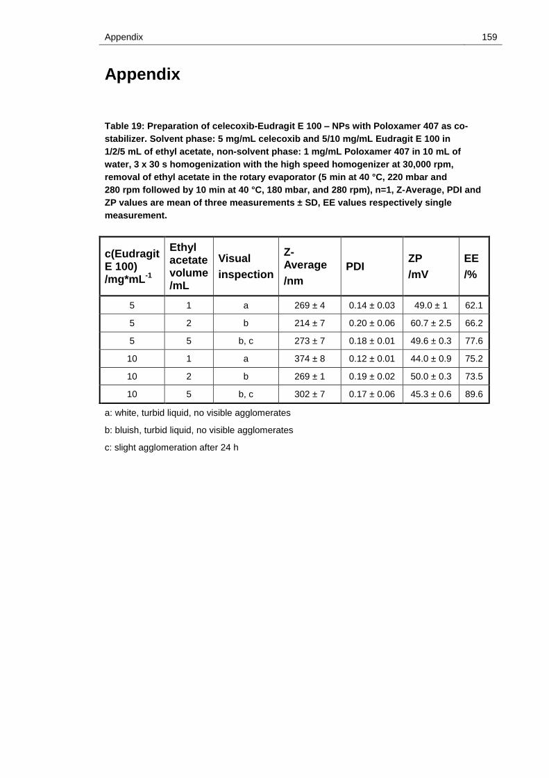
Appendix 159

Appendix

Table 19: Preparation of celecoxib-Eudragit E 100 – NPs with Poloxamer 407 as co-

stabilizer. Solvent phase: 5 mg/mL celecoxib and 5/10 mg/mL Eudragit E 100 in

1/2/5 mL of ethyl acetate, non-solvent phase: 1 mg/mL Poloxamer 407 in 10 mL of

water, 3 x 30 s homogenization with the high speed homogenizer at 30,000 rpm,

removal of ethyl acetate in the rotary evaporator (5 min at 40 °C, 220 mbar and

280 rpm followed by 10 min at 40 °C, 180 mbar, and 280 rpm), n=1, Z-Average, PDI and

ZP values are mean of three measurements ± SD, EE values respectively single

measurement.

c(Eudragit E 100) /mg*mL-1

Ethyl acetate volume /mL

Visual

inspection

Z-Average

/nm

PDI ZP

/mV

EE

/%

5 1 a 269 ± 4 0.14 ± 0.03 49.0 ± 1 62.1

5 2 b 214 ± 7 0.20 ± 0.06 60.7 ± 2.5 66.2

5 5 b, c 273 ± 7 0.18 ± 0.01 49.6 ± 0.3 77.6

10 1 a 374 ± 8 0.12 ± 0.01 44.0 ± 0.9 75.2

10 2 b 269 ± 1 0.19 ± 0.02 50.0 ± 0.3 73.5

10 5 b, c 302 ± 7 0.17 ± 0.06 45.3 ± 0.6 89.6

a: white, turbid liquid, no visible agglomerates

b: bluish, turbid liquid, no visible agglomerates

c: slight agglomeration after 24 h

160 Appendix

Table 20: Preparation of celecoxib-Eudragit E 100 – NPs with SDS as co-stabilizer.

Solvent phase: 5 mg/mL celecoxib and 5/10 mg/mL Eudragit E 100 in 1/2/5 mL of ethyl

acetate, non-solvent phase: 1 mg/mL SDS in 10 mL of water, 3 x 30 s homogenization

with the high speed homogenizer at 30,000 rpm, removal of ethyl acetate in the rotary

evaporator (5 min at 40 °C, 220 mbar and 280 rpm followed by 10 min at 40 °C,

180 mbar, and 280 rpm), n=1, Z-Average, PDI and ZP values are mean of three

measurements ± SD, EE values respectively single measurement.

c(Eudragit E 100) /mg*mL-1

Ethyl acetate volume /mL

Visual

inspection

Z-Average

/nm PDI

ZP

/mV

EE

/%

5 1 a 260 ± 17 0.27 ± 0.11 - 11 ± 0.4 95.4

5 2 a 552 ± 86 0.13 ± 0.12 4.4 ± 0.2 95.5

5 5 a, b 393 ± 6 0.06 ± 0.04 39.2 ± 1.1 99.7

10 1 a 825 ± 74 0.15 ± 0.02 2.7 ± 0.5 88.5

10 2 a 205 ± 5 0.03 ± 0.02 27.1 ± 0.6 99.0

10 5 a, b 7,205 ± 2,069 0.67 ± 0.27 51.8 ± 1.3 99.8

a: appearance of large agglomerates

b: crystallization after 24 h, no visible turbidity

Appendix 161

Table 21: Preparation of celecoxib-Eudragit E 100 – NPs with PVA (MW: 27,000) as co-

stabilizer. Solvent phase: 5 mg/mL celecoxib and 5/10 mg/mL Eudragit E 100 in

1/2/5 mL of ethyl acetate, non-solvent phase: 1 mg/mL PVA in 10 mL of water, 3 x 30 s

homogenization with the high speed homogenizer at 30,000 rpm, removal of ethyl

acetate in the rotary evaporator (5 min at 40 °C, 220 mbar and 280 rpm followed by

1 min at 40 °C, 180 mbar, and 280 rpm), n=1, Z-Average, PDI and ZP values are mean

of three measurements ± SD, EE values respectively single measurement.

c(Eudragit E 100) /mg*mL-1

Ethyl acetate volume /mL

Visual

inspection

Z-Average

/nm PDI

ZP

/mV

EE

/%

5 1 a, b 278 ± 74 0.49 ± 0.14 - 3.8 ± 1.3 7.7

5 2 a, b 548 ± 214 0.77 ± 0.20 2.5 ± 0.8 13.5

5 5 a, b 31,183 ± 14,732

0.94 ± 0.11 11.3 ± 1.6 36.5

10 1 a, b 484 ± 32 0.47 ± 0.04 1.9 ± 0.2 34.4

10 2 a, b 431 ± 155 0.74 ± 0.16 2.1 ± 1.1 14.6

10 5 a, b 982 ± 321 0.87 ± 0.19 4.1 ± 0.5 39.3

a: appearance of large agglomerates

b: suspension not turbid

162 Appendix

Table 22: Preparation of celecoxib-Eudragit E 100 – NPs with varying amounts of

Poloxamer 407. Solvent phase: 5 mg/mL celecoxib and 10 mg/mL Eudragit E 100 in

2 mL of ethyl acetate, non-solvent phase: 0.1/0.5/1/2.5/5/10 mg/mL Poloxamer 407 in

10 mL of water, 3 x 30 s homogenization with the high speed homogenizer at

30,000 rpm, removal of ethyl acetate in the rotary evaporator (5 min at 40 °C, 220 mbar

and 280 rpm followed by 10 min at 40 °C, 180 mbar, and 280 rpm), n=3, values are

mean ± SD.

c

(Poloxamer 407)

/mg*mL-1

Visual

inspection

Z-Average

/nm PDI

ZP

/mV

EE

/%

0.1 a 417 ± 38 0.26 ± 0.01 50 ± 3 94.6 ± 0

0.5 a 315 ± 17 0.28 ± 0.01 49 ± 1 84.0 ± 3

1 a 254 ± 17 0.17 ± 0.03 46 ± 4 75.7 ± 3

2.5 b 215 ± 11 0.05 ± 0.01 39 ± 2 72.3 ± 5

5 c 204 ± 5 0.05 ± 0.02 31 ± 1 61.4 ± 3

10 c 199 ± 3 0.07 ± 0.03 29 ± 0 51.6 ± 2

a: white, turbid liquid, sediments on the flask wall

b: white, turbid liquid

c: white, slightly bluish, turbid liquid

Appendix 163

Table 23: Stability study of celecoxib-Eudragit E 100 – NPs stabilized with

Poloxamer 407: Solvent phase: 5 mg/mL celecoxib and 10 mg/mL Eudragit E 100 in

2 mL of ethyl acetate, non-solvent phase: 2.5 mg/mL Poloxamer 407 in 10 mL of water,

3 x 30 s homogenization with the high speed homogenizer at 30,000 rpm, removal of

ethyl acetate in the rotary evaporator (5 min at 40 °C, 220 mbar and 280 rpm followed

by 10 min at 40 °C, 180 mbar, and 280 rpm), stored at room temperature, n=3, values

are mean ± SD.

Storage

/d

Z-Average

/nm PDI

ZP

/mV

EE

/%

0 223 ± 5 0.10 ± 0.03 38.2 ± 4.3 72.2 ± 3.6

1 214 ± 6 0.11 ± 0.04 36.8 ± 5.3 70.0 ± 6.6

2 222 ± 8 0.15 ± 0.06 43.3 ± 1.2 72.0 ± 11.0

3 226 ± 9 0.19 ± 0.06 51.8 ± 4.3 76.2 ± 11.6

4 237 ± 10 0.23 ± 0.09 53.2 ± 2.0 73.1 ± 6.2

7 265 ± 34 0.33 ± 0.16 61.0 ± 0.7 80.2 ± 5.5

14 263 ± 52 0.32 ± 0.14 55.9 ± 2.3 70.2 ± 8.6

Table 24: Stability study of celecoxib-Eudragit E 100 – NPs stabilized with

Poloxamer 407: Solvent phase: 5 mg/mL celecoxib and 10 mg/mL Eudragit E 100 in

2 mL of ethyl acetate, non-solvent phase: 2.5 mg/mL Poloxamer 407 in 10 mL of water,

3 x 30 s homogenization with the high speed homogenizer at 30,000 rpm, removal of

ethyl acetate in the rotary evaporator (5 min at 40 °C, 220 mbar and 280 rpm followed

by 10 min at 40 °C, 180 mbar, and 280 rpm), stored at 5 °C, n=3, values are mean ± SD.

Storage

/d

Z-Average

/nm PDI

ZP

/mV

EE

/%

0 223 ± 5 0.10 ± 0.03 38.2 ± 4.3 72.2 ± 3.6

1 211 ± 2 0.09 ± 0.03 39.7 ± 0.9 72.0 ± 0.1

2 218 ± 4 0.16 ± 0.08 41.0 ± 1.5 76.2 ± 2.4

3 214 ± 3 0.14 ± 0.03 44.3 ± 1.1 83.3 ± 1.1

4 254 ± 19 0.32 ± 0.06 47.8 ± 1.9 80.3 ± 1.0

7 278 ± 53 0.33 ± 0.15 55.9 ± 2.0 69.7 ± 1.9

14 249 ± 36 0.21 ± 0.08 51.6 ± 0.8 65.0 ± 10.5

164 Appendix

Table 25: Stability study of celecoxib-Eudragit E 100 – NPs stabilized with

Poloxamer 407: Solvent phase: 25 mg/mL celecoxib and 50 mg/mL Eudragit E 100 in

2 mL of ethyl acetate, non-solvent phase: 12.5 mg/mL Poloxamer 407 in 10 mL of

water, 3 x 30 s homogenization with the high speed homogenizer at 30,000 rpm,

removal of ethyl acetate in the rotary evaporator (5 min at 40 °C, 220 mbar and

280 rpm followed by 10 min at 40 °C, 180 mbar, and 280 rpm), stored at room

temperature, n=3, values are mean ± SD.

Storage

/d

Z-Average

/nm PDI

ZP

/mV

EE

/%

0 290 ± 7 0.12 ± 0.02 39.4 ± 0.6 85.6 ± 4.3

1 276 ± 6 0.15 ± 0.04 38.3 ± 0.2 83.2 ± 0.5

2 280 ± 10 0.08 ± 0.02 40.6 ± 2.2 81.0 ± 1.5

3 280 ± 6 0.11 ± 0.03 42.5 ± 0.8 80.3 ± 2.5

4 284 ± 7 0.11 ± 0.01 44.3 ± 0.5 81.3 ± 10.2

7 277 ± 6 0.08 ± 0.04 51.7 ± 4.0 80.3 ± 1.8

14 241 ± 8 0.09 ± 0.02 46.1 ± 0.5 84.6 ± 1.0

Table 26: Stability study of celecoxib-Eudragit E 100 – NPs stabilized with

Poloxamer 407: Solvent phase: 25 mg/mL celecoxib and 50 mg/mL Eudragit E 100 in

2 mL of ethyl acetate, non-solvent phase: 12.5 mg/mL Poloxamer 407 in 10 mL of

water, 3 x 30 s homogenization with the high speed homogenizer at 30,000 rpm,

removal of ethyl acetate in the rotary evaporator (5 min at 40 °C, 220 mbar and

280 rpm followed by 10 min at 40 °C, 180 mbar, and 280 rpm), stored at 5 °C, n=3,

values are mean ± SD.

Storage

/d

Z-Average

/nm PDI

ZP

/mV

EE

/%

0 290 ± 7 0.12 ± 0.02 39.4 ± 0.6 85.6 ± 4.3

1 275 ± 5 0.14 ± 0.04 37.1 ± 0.7 83.3 ± 3.0

2 284 ± 6 0.12 ± 0.02 38.9 ± 0.7 82.2 ± 3.4

3 278 ± 6 0.14 ± 0.04 42.3 ± 0.5 80.1 ± 3.5

4 354 ± 66 0.37 ± 0.24 42.9 ± 2.4 85.1 ± 1.4

7 380 ± 77 0.45 ± 0.18 55.2 ± 0.9 84.9 ± 0.9

14 252 ± 12 0.18 ± 0.03 45.2 ± 1.1 87.0 ± 3.3

Appendix 165

Table 27: Stability study of celecoxib-Eudragit E 100 – NPs stabilized with

Poloxamer 407: t-test for comparison of storage at room temperature versus storage

at 5 °C and usage of 5 mg/mL versus 25 mg/mL celecoxib in solvent phase, data rows

from days 0 to 14 are respectively compared.

Comparison Parameter p-value

5 mg/mL_RT

versus

5 mg/mL_5 °C

Z-Average 0.9708

PDI 0.8023

ZP 0.4839

EE 0.8069

25 mg/mL_RT

versus

25 mg/mL_5 °C

Z-Average 0.1799

PDI 0.0561

ZP 0.9180

EE 0.1800

5 mg/mL_RT

versus

25 mg/mL_RT

Z-Average 0.0016

PDI 0.0214

ZP 0.1985

EE 0.0001

5 mg/mL_5 °C

versus

25 mg/mL_5 °C

Z-Average 0.0061

PDI 0.7014

ZP 0.4703

EE 0.0021

166 Appendix

Table 28: MJR preparation of celecoxib-Eudragit E 100 – NPs stabilized with

Poloxamer 407 using DoE: Solvent phase: 25 mg/mL celecoxib and 50 mg/mL

Eudragit E 100 in ethyl acetate, non-solvent phase: 12.5 mg/mL Poloxamer 407 in

water, operation temperature: 40-60 °C, nitrogen pressure: 0-0.50 bar, pump rotational

speed (solvent phase : non-solvent phase) 300 : 1500 rpm to 1200 : 6000 rpm, removal

of remaining ethyl acetate by evaporating for 18 h in the fume hood, values are mean

of three measurements.

Run Temperature /°C

Nitrogen pressure

/bar

Pump rotational speed

/rpm

Z-Average

/nm PDI

1 60.0 0.25 1200 : 6000 263.6 0.157

2 60.0 0.25 300 : 1500 539.3 0.352

3 60.0 0.50 750 : 3750 297.7 0.14

4 50.0 0.50 300 : 1500 369.6 0.08

5 40.0 0.50 750 : 3750 286 0.145

6 40.0 0 750 : 3750 283.2 0.163

7 50.0 0 300 : 1500 746.9 1

8 50.0 0.25 750 : 3750 320.5 0.259

9 50.0 0.25 750 : 3750 327.4 0.249

10 50.0 0.50 1200 : 6000 549.5 0.836

11 50.0 0.25 750 : 3750 301.2 0.164

12 60.0 0 750 : 3750 359 0.101

13 40.0 0.25 1200 : 6000 420 0.46

14 40.0 0.25 300 : 1500 331.6 0.157

15 50.0 0 1200 : 6000 294.3 0.103

16 50.0 0.25 750 : 3750 292.8 0.06

17 50.0 0.25 750 : 3750 560.1 0.804

Appendix 167

Table 29: MJR preparation of celecoxib-Eudragit E 100 – NPs stabilized with

Poloxamer 407, validation of DoE model: Solvent phase: 25 mg/mL celecoxib and

50 mg/mL Eudragit E 100 in ethyl acetate, non-solvent phase: 12.5 mg/mL

Poloxamer 407 in water, operation temperature: 55-59 °C, nitrogen pressure: 0.31-

0.47 bar, pump rotational speed (solvent phase : non-solvent phase) 300 : 1500 rpm to

719 : 3595 rpm, removal of remaining ethyl acetate by evaporating for 18 h in the fume

hood, n=1, Z-Average, PDI and ZP values are mean of three measurements ± SD, EE

values respectively single measurement.

Experimental conditions

Z-Average

(predicted value)

/nm

Z-Average

(actual value)

/nm

PDI ZP

/mV

EE

/%

57.4 °C_0.39 bar_

719 : 3595 rpm 300 287.5 ± 2.4 0.156 ± 0.045 41.9 ± 0.3 84.3

58.4 °C_0.40 bar_

510 : 2550 rpm 350 330.6 ± 3.0 0.081 ± 0.066 46.2 ± 1.0 86.5

56.0 °C_0.45 bar_

491 : 2455 rpm 350 331.3 ± 26.5 0.126 ± 0.057 44.1 ± 1.0 88.3

55.0 °C_0.31 bar_

571 : 2855 rpm 350 364.3 ± 9.3 0.086 ± 0.057 43.5 ± 0.9 91.2

58.1 °C_0.32 bar_

457 : 2285 rpm 400 396.7 ± 6.6 0.219 ± 0.077 44.4 ± 0.2 81.0

56.2 °C_0.47 bar_

349 : 1745 rpm 400 431.6 ± 15.4 0.146 ± 0.077 45.3 ± 0.5 83.7

55.8 °C_0.35 bar_

433 : 2165 rpm 400 380.1 ± 11.8 0.144 ± 0.075 47.2 ± 2.1 90.4

55.7 °C_0.41 bar_

300 : 1500 rpm 450 442.7 ± 20.0 0.223 ± 0.078 44.0 ± 1.0 85.4

57.5 °C_0.40 bar_

313 : 1565 rpm 450 444.3 ± 23.4 0.168 ± 0.092 43.7 ± 3.4 87.7

59.0 °C_0.36 bar_

350 : 1750 rpm 450 505.6 ± 9.7 0.202 ± 0.074 44.6 ± 3.5 82.3

168 Appendix

Table 30: Dissolution of celecoxib-Eudragit E 100-NPs in HCl pH 1.2: NP properties:

80 nm (Z-Average), 0.131 (PDI) and 2.573 mg/mL (celecoxib concentration of the

nanosuspension), detection: UV-Vis (248 nm), n=3, values are mean ± SD.

Sampling point

/min 3 6 9 12 15 18 21 30 60 120

API dissolved

/%

HCl pH 1.2

22.1

±

12.0

47.1

±

3.8

53.8

±

3.4

53.9

±

6.3

51.9

±

7.3

49.5

±

7.7

47.0

±

7.3

40.6

±

4.4

34.3

±

4.2

33.5

±

1.7

Table 31: Dissolution of celecoxib-Eudragit E 100-NPs in diluted HCl pH 1.2 + 0.15 M

NaCl: NP properties: 100 nm (Z-Average), 0.100 (PDI) and 2.331 mg/mL (celecoxib

concentration of the nanosuspension), detection: UV-Vis (248 nm), n=1.

Sampling point

/min 3 6 9 12 15 18 21 30 60 120

API dissolved

/%

HCl pH 1.2 + 0.15 M NaCl

13.1 30.6 34.7 35.3 34.1 32.1 29.5 23.9 18.0 5.0

Appendix 169

Table 32: Dissolution of celecoxib-Eudragit E 100-NPs in diluted HCl pH 1.2 +

0.001/0.01/0.3/1.0 % cetrimide: NP properties: 80 nm (Z-Average), 0.131 (PDI) and

2.573 mg/mL (celecoxib concentration of the nanosuspension), detection: UV-Vis

(248 nm), n=1.

Sampling point

/min 3 6 9 12 15 18 21 30 60 120

AP

I d

iss

olv

ed

/%

HCl pH 1.2 + 0.001 % cetrimide

0.5 15.2 14.2 11.8 10.6 9.8 9.5 8.9 8.2 7.4

HCl pH 1.2 + 0.01 % cetrimide

3.2 4.9 7.9 9.8 10.7 11.1 11.3 11.3 10.8 10.1

HCl pH 1.2 + 0.3 % cetrimide

4.8 5.5 5.9 6.2 6.4 7.2 7.5 7.9 10.0 12.9

HCl pH 1.2 + 1.0 % cetrimide

4.5 5.3 5.2 5.6 5.5 6.1 6.6 7.0 7.3 8.2

Table 33: Dissolution of celecoxib-Eudragit E 100-NPs in diluted HCl pH 1.2 + 0.3 %

cetrimide: NP properties: 160 nm (Z-Average), 0.094 (PDI) and 2.388 mg/mL (celecoxib

concentration of the nanosuspension), filters: cross-flow filtration modules of 100 and

500 kDa and 0.2 µm syringe filter holders (dead-end), detection: UV-Vis (248 nm), n=3,

values are mean ± SD.

Sampling point

/min 3 6 9 12 15 18 21 30 60 120

AP

I d

iss

olv

ed

/%

100 kDa cross-flow

3.7 ±

0.6

5.9 ±

0.5

6.8 ±

0.7

7.1 ±

0.3

7.4 ±

0.4

7.7 ±

0.2

7.6 ±

0.6

7.8 ±

0.7

8.3 ±

0.7

9.0 ±

0.6

500 kDa cross-flow

96.6 ±

5.1

95.7 ±

0.4

95.8 ±

0.5

96.3 ±

1.1

96.8 ±

1.1

96.3 ±

1.7

97.2 ±

2.6

97.4 ±

2.7

98.9 ±

3.1

101.4 ±

3.7

0.2 µm dead-end

95.6 ±

1.3

98.2 ±

0.6

99.1 ±

0.7

98.0 ±

2.9

99.5 ±

2.4

99.1 ±

1.0

101.0 ± 1.9

101.3 ± 1.4

100.8 ±

0.4

101.1 ±

1.0

170 Appendix

Table 34: Dissolution of celecoxib-Eudragit E 100-NPs in diluted HCl pH 1.2 + 0.05 %

cetrimide: NP properties: 160 nm (Z-Average), 0.094 (PDI) and 2.509 mg/mL (celecoxib

concentration of the nanosuspension), filters: cross-flow filtration modules of 100 and

500 kDa and 0.2 µm syringe filter holders (dead-end), detection: UV-Vis (248 nm), n=3,

values are mean ± SD.

Sampling point

/min 3 6 9 12 15 18 21 30 60 120

AP

I d

iss

olv

ed

/%

100 kDa cross-flow

1.0 ±

1.1

9.0 ±

1.1

12.1 ±

1.5

12.9 ±

1.3

13.6 ±

1.9

13.7 ±

1.3

13.4 ±

0.6

13.3 ±

1.0

13.4 ±

0.7

14.0 ±

0.4

500 kDa cross-flow

78.4 ±

1.8

81.3 ±

2.6

82.1 ±

2.5

82.2 ±

2.3

82.8 ±

2.1

83.2 ±

2.1

83.9 ±

2.6

84.8 ±

2.7

85.5 ±

3.0

86.7 ±

3.6

0.2 µm dead-end

71.8 ±

2.3

78.1 ±

3.4

82.2 ±

2.6

83.6 ±

2.6

86.4 ±

1.6

86.8 ±

1.5

87.3 ±

1.3

88.0 ±

1.2

88.0 ±

1.7

88.6 ±

0.8

Table 35: Dissolution of celecoxib-Eudragit E 100-NPs in phosphate buffer

pH 2.0/2.5/3.5/4.5/5.2+ 0.3 % cetrimide: NP properties: 220 nm (Z-Average), 0.086 (PDI)

and 3.666 mg/mL (celecoxib concentration of the nanosuspension), filter: 500 kDa

cross-flow filtration module, detection: UV-Vis (248 nm), n=3, values are mean ± SD.

Sampling point

/min

3 6 9 12 15 18 21 30 45 60 120

AP

I d

iss

olv

ed

/%

pH 2.0

81.0 ±

1.5

80.9 ±

1.1

81.4 ±

1.2

81.6 ±

1.1

82.2 ±

0.8

82.7 ±

0.6

83.0 ±

0.7

83.6 ±

0.5

84.6 ±

0.5

85.4 ±

0.9

88.8 ±

1.2

pH 2.5

74.6 ±

1.5

76.1 ±

1.0

77.1 ±

1.5

77.5 ±

1.6

78.0 ±

1.4

78.4 ±

1.3

78.8 ±

1.2

79.3 ±

1.7

79.7 ±

1.3

80.3 ±

1.8

83.4 ±

0.7

pH 3.5

64.5 ±

1.6

65.6 ±

1.3

66.0 ±

1.6

66.4 ±

2.2

66.7 ±

2.4

67.2 ±

2.6

67.3 ±

2.3

67.4 ±

2.2

67.7 ±

1.9

68.1 ±

2.1

69.7 ±

1.9

pH 4.5

36.6 ±

1.5

38.1 ±

0.8

39.0 ±

0.6

40.0 ±

0.8

40.6 ±

1.1

41.1 ±

1.0

41.4 ±

0.8

42.5 ±

1.3

43.4 ±

1.5

44.6 ±

1.8

46.8 ±

2.1

pH 5.2

23.0 ±

4.6

25.2 ±

4.6

26.5 ±

4.1

27.1 ±

4.2

27.6 ±

3.9

28.2 ±

4.1

28.6 ±

3.8

29.2 ±

3.8

30.2 ±

3.4

30.8 ±

3.8

32.4 ±

3.6

Appendix 171

Table 36: Dissolution of celecoxib-Eudragit E 100-NPs of different size and celecoxib

powder in phosphate buffer pH 2.0 + 0.3 % cetrimide: NP properties:

221/255/293/362/497 nm (Z-Average), < 0.25 (PDI) and ~ 2.650–4.850 mg/mL (celecoxib

concentration of the nanosuspension), API powder: 2537 µg/mL (celecoxib

concentration of the suspension), filter: 500 kDa cross-flow filtration module,

detection: UV-Vis (248 nm), n=6, values are mean ± SD.

Sampling point

/s 20 40 60 90 120 900 1800 3600

AP

I d

iss

olv

ed

/%

221 nm

8.6

±

6.3

79.2

±

1.8

85.5

±

0.9

85.8

±

0.7

85.4

±

0.9

- - -

255 nm

13.4

±

8.3

82.1

±

1.8

87.0

±

1.2

86.7

±

0.9

86.1

±

1.1

- - -

293 nm

13.4

±

8.1

78.0

±

15.3

86.0

±

10.5

89.8

±

3.4

90.4

±

2.8

- - -

362 nm

13.8

±

17.1

79.3

±

4.8

87.2

±

4.8

89.3

±

4.5

90.3

±

4.3

- - -

497 nm

12.2

±

5.1

77.5

±

4.2

84.6

±

3.5

85.0

±

4.1

83.9

±

3.6

- - -

API powder

0.8

±

2.0

24.7

±

3.1

41.0

±

5.4

55.4

±

8.5

63.7

±

10.2

80.8

±

13.3

82.0

±

13.1

84.5

±

12.6

172 Appendix

Figure 64: SEM image of MJR produced celecoxib-Eudragit E 100-particles

(nanoprecipitation technique): NP properties (determined by DLS, mean of three

measurements): 1156 nm (Z-Average), 0.144 (PDI).

Figure 65: SEM image of MJR produced celecoxib-Eudragit E 100-NPs

(nanoprecipitation technique): NP properties (determined by DLS, mean of three

measurements): 387 nm (Z-Average), 0.285 (PDI).

Appendix 173

Figure 66: SEM image of MJR produced celecoxib-Eudragit E 100-NPs (emulsification-

diffusion technique): NP properties (determined by DLS, mean of three

measurements): 611 nm (Z-Average), 0.258 (PDI).

Figure 67: SEM image of MJR produced celecoxib-Eudragit E 100-NPs (emulsification-

diffusion technique): NP properties (determined by DLS, mean of three

measurements): 254 nm (Z-Average), 0.148 (PDI).

174 Appendix

Figure 68: DLS size distribution reports (volume-weighted) of celecoxib-

Eudragit E 100-NPs; NP-preparation: nanoprecipitation technique–alternative method,

non-solvent phase without surfactant, see chapter 2.2.1.2; unfiltered nanosuspension

(a) versus liquid obtained from filtration of this nanosuspension through a 500 kDa CF

module (b) and from filtration through a syringe filter holder with 0.2 µm pore size (c);

NP properties: 160 nm (Z-Average), 0.094 (PDI).

Appendix 175

Figure 69: Simulation of the NP dissolution process in dissolution medium: DLS size

distribution reports (volume-weighted) of celecoxib-Eudragit E 100-NPs; same

nanosuspension as in Figure 68, but respectively measured at 37 °C (dissolution test

temperature); 1:100 aqueous dilution of the nanosuspension (a) versus 1:100 dilution

in 0.1 M HCl + 0.3 % cetrimide after 15 min incubation time in the cuvette of the DLS

instrument (b).

176 Appendix

Figure 70: Laser light diffraction size distribution report of unprocessed celecoxib

particles; density distribution and cumulative distribution; volume-weighted median

diameter (VMD) in red rectangle.

Appendix 177

Figure 71: DLS size distribution reports (volume-weighted) of two dissolution media:

HCl pH 1.2 + 0.05 % cetrimide (a) and HCl pH 1.2 + 0.3 % cetrimide (with micelles) (b).

178 References

References

[1] M.M.A. Abdel-Mottaleb, N.D. Mortada, A.A. El-Shamy, G.A.S. Awad, Physically cross-linked polyvinyl alcohol for the topical delivery of fluconazole, Drug Dev Ind Pharm 35 (2009) 311–320.

[2] M.M.A. Abdel-Mottaleb, D. Neumann, A. Lamprecht, In vitro drug release mechanism from lipid nanocapsules (LNC), Int J Pharm 390 (2010) 208–213.

[3] W. Abdelwahed, G. Degobert, S. Stainmesse, H. Fessi, Freeze-drying of nanoparticles: formulation, process and storage considerations, Adv Drug Deliver Rev 58 (2006) 1688–1713.

[4] J. Albers, Hot-melt extrusion with poorly soluble drugs. Ph.D. Thesis, Düsseldorf, 2008.

[5] J. Albers, R. Alles, K. Matthée, K. Knop, J.S. Nahrup, P. Kleinebudde, Mechanism of drug release from polymethacrylate-based extrudates and milled strands prepared by hot-melt extrusion, Eur J Pharm Biopharm 71 (2009) 387–394.

[6] G.L. Amidon, H. Lennernäs, V.P. Shah, J.R. Crison, A theoretical basis for a biopharmaceutic drug classification: the correlation of in vitro drug product dissolution and in vivo bioavailability, Pharm Res 12 (1995) 413–420.

[7] A.N. Ananth, S.C.G.K. Daniel, T.A. Sironmani, S. Umapathi, PVA and BSA stabilized silver nanoparticles based surface-enhanced plasmon resonance probes for protein detection, Colloid Surface B 85 (2011) 138–144.

[8] G. Askarieh, M. Hedhammar, K. Nordling, A. Saenz, C. Casals, A. Rising, J. Johansson, S.D. Knight, Self-assembly of spider silk proteins is controlled by a pH-sensitive relay, Nature 465 (2010) 236–238.

[9] M. Baalousha, J. Lead, Characterization of natural and manufactured nanoparticles by atomic force microscopy: Effect of analysis mode, environment and sample preparation, Colloid Surface A 419 (2013) 238–247.

[10] S. Baboota, S. Faiyaz, Ahuja A., Ali J., Shafiq S., S. Ahmad, Development and validation of stability-indicating HPLC method for analysis of Celecoxib (CXB) in bulk drug and microemulsion formulations, Acta Chromatogr (2007) 116–129.

[11] Y. Barenholz, Doxil®--the first FDA-approved nano-drug: lessons learned, J Control Release 160 (2012) 117–134.

[12] T.R. Bates, M. Gibaldi, J.L. Kanig, Rate of dissolution of griseofulvin and hexoestrol in bile salt solutions, Nature 210 (1966) 1331–1333.

[13] K.H. Bauer, B.C. Lippold, H. Egermann, Lehrbuch der Pharmazeutischen Technologie: Mit einer Einführung in die Biopharmazie ; 95 Tabellen, 8 ed., Wissenschaftliche Verlagsgesellschaft, Stuttgart, 2006.

[14] U. Bilati, E. Allémann, E. Doelker, Development of a nanoprecipitation method intended for the entrapment of hydrophilic drugs into nanoparticles, Eur J Pharm Sci 24 (2005) 67–75.

[15] G. Binnig, C.F. Quate, C. Gerber, Atomic Force Microscope, Phys Rev Lett 56 (1986) 930–934.

References 179

[16] G. Bisker, D. Yeheskely-Hayon, L. Minai, D. Yelin, Controlled release of Rituximab from gold nanoparticles for phototherapy of malignant cells, J Control Release 162 (2012) 303–309.

[17] BMBF, Nanopartikel - kleine Dinge, große Wirkung, 2008, http://www.bmbf.de/pub/nanopartikel_kleine_dinge_grosse_wirkung.pdf, accessed 15 April 2013.

[18] A. Bohr, J. Kristensen, E. Stride, M. Dyas, M. Edirisinghe, Preparation of microspheres containing low solubility drug compound by electrohydrodynamic spraying, Int J Pharm 412 (2011) 59–67.

[19] C.A. Bunton, F. Nome, F.H. Quina, L.S. Romsted, Ion Binding and Reactivity at Charged Aqueous Interfaces, Acc. Chem. Res. (Accounts of Chemical Research) 24 (1991) 357–364.

[20] Carl Zeiss Microscopy, ZEISS EVO Your High Definition SEM with Workflow Automation: Product Information Version 1.0, 2013, http://applications.zeiss.com/C125792900358A3F/0/A7A32858228B4D46C1257BBB004E6E74/$FILE/EN_42_011_092_EVO.pdf, accessed 9 October 2013.

[21] H.-K. Chan, P.C.L. Kwok, Production methods for nanodrug particles using the bottom-up approach, Adv Drug Deliv Rev 63 (2011) 406–416.

[22] X. Chen, J.M. Vaughn, M.J. Yacaman, R.O. Williams, K.P. Johnston, Rapid dissolution of high-potency danazol particles produced by evaporative precipitation into aqueous solution, J Pharm Sci 93 (2004) 1867–1878.

[23] Y. Chen, Y. Lu, J. Chen, J. Lai, J. Sun, F. Hu, W. Wu, Enhanced bioavailability of the poorly water-soluble drug fenofibrate by using liposomes containing a bile salt, Int J Pharm 376 (2009) 153–160.

[24] K.Y. Choi, K.H. Min, H.Y. Yoon, K. Kim, J.H. Park, I.C. Kwon, K. Choi, S.Y. Jeong, PEGylation of hyaluronic acid nanoparticles improves tumor targetability in vivo, Biomaterials 32 (2011) 1880–1889.

[25] C. Colliex, H. Kohl, Elektronenmikroskopie: Eine anwendungsbezogene Einführung, Wiss. Verlagsges., Stuttgart, 2008.

[26] E.R. Cooper, Nanoparticles: A personal experience for formulating poorly water soluble drugs, J Control Release 141 (2010) 300–302.

[27] D.Q.M. Craig, The mechanisms of drug release from solid dispersions in water-soluble polymers, Int J Pharm 231 (2002) 131–144.

[28] S.M. D'Addio, R.K. Prud'homme, Controlling drug nanoparticle formation by rapid precipitation, Adv Drug Deliv Rev 63 (2011) 417–426.

[29] S. Das, P.K. Suresh, R. Desmukh, Design of Eudragit RL 100 nanoparticles by nanoprecipitation method for ocular drug delivery, Nanomedicine 6 (2010) 318–323.

[30] J. Deng, L. Huang, F. Liu, Understanding the structure and stability of paclitaxel nanocrystals, Int J Pharm 390 (2010) 242–249.

[31] B. Derjaguin, L. Landau, Theory of the stability of strongly charged lyophobic sols and of the adhesion of strongly charged particles in solutions of electrolytes, Prog Surf Sci 43 (1993) 30–59.

[32] A. Dokoumetzidis, P. Macheras, A century of dissolution research: from Noyes and Whitney to the biopharmaceutics classification system, Int J Pharm 321 (2006) 1–11.

[33] A. Dolenc, J. Kristl, S. Baumgartner, O. Planinšek, Advantages of celecoxib nanosuspension formulation and transformation into tablets, Int J Pharm 376 (2009) 204–212.

180 References

[34] A. Dominik, D. Steinhilber, Instrumentelle Analytik: Kurzlehrbuch und kommentierte Originalfragen für Pharmazeuten, 2 ed., Dt. Apotheker-Verl., Stuttgart, 2002.

[35] J.L. Dubois, J.L. Ford, Similarities in the release rates of different drugs from polyethylene glycol 6000 solid dispersions, J Pharm Pharmacol 37 (1985) 494–495.

[36] L. Edwards, The dissolution and diffusion of aspirin in aqueous media, Trans Faraday Soc (1951) 1191–1210.

[37] J.M. Edwardson, R.M. Henderson, Atomic force microscopy and drug discovery, Drug Discov Today 9 (2004) 64–71.

[38] M.H. El-Shabouri, Positively charged nanoparticles for improving the oral bioavailability of cyclosporin-A, Int J Pharm 249 (2002) 101–108.

[39] A.H. Elshafeey, A.O. Kamel, G.A. Awad, Ammonium methacrylate units polymer content and their effect on acyclovir colloidal nanoparticles properties and bioavailability in human volunteers, Colloid Surface B 75 (2010) 398–404.

[40] Evonik Industries AG, Eudragit E 100 Product Information, http://eudragit.evonik.com/product/eudragit/en/products-services/eudragit-products/protective-formulations/e-100/Pages/default.aspx, accessed 31 May 2014.

[41] H.M. Fadda, H.A. Merchant, B.T. Arafat, A.W. Basit, Physiological bicarbonate buffers: stabilisation and use as dissolution media for modified release systems, Int J Pharm 382 (2009) 56–60.

[42] T. Feczkó, J. Tóth, G. Dósa, J. Gyenis, Influence of process conditions on the mean size of PLGA nanoparticles, Chem Eng Process 50 (2011) 846–853.

[43] H. Fessi, J.-P. Devissaguet, F. Puisieux, C. Thies, Process for the preparation of dispersible colloidal systems of a substance in the form of nanoparticles, United States Patent 5118528 (1990).

[44] H. Fessi, F. Puisieux, J. Devissaguet, N. Ammoury, S. Benita, Nanocapsule formation by interfacial polymer deposition following solvent displacement, Int J Pharm 55 (1989) R1-R4.

[45] J. Finholt, Influence of formulation on dissolution rate, in: L. Leeson, J. Carstensen (Eds.), Dissolution Technology, Washington, DC, 1974, pp. 106–146.

[46] B. Finn, CELEBREX ® (celecoxib) capsules, 1998, http://labeling.pfizer.com/ShowLabeling.aspx?id=793, accessed 16 April 2013.

[47] B. Finn, HIGHLIGHTS OF PRESCRIBING INFORMATION, 2013, http://labeling.pfizer.com/ShowLabeling.aspx?id=793, accessed 16 January 2013.

[48] E.J. Fraser, R.H. Leach, J.W. Poston, A.M. Bold, L.S. Culank, A.B. Lipede, Dissolution-rates and bioavailability of digoxin tablets, Lancet 1 (1973) 1393.

[49] C. Freitas, R.H. Müller, Spray-drying of solid lipid nanoparticles (SLN TM), Eur J Pharm Biopharm 46 (1998) 145–151.

[50] A. Frick, C. Stern, DSC-Prüfung in der Anwendung, Hanser, München, Wien, 2006.

[51] J. Gajendran, J. Kraemer, P. Langguth, In vivo predictive release methods for medicated chewing gums, Biopharmaceutics & drug disposition 33 (2012) 417–424.

References 181

[52] E. Galia, E. Nicolaides, D. Hörter, R. Löbenberg, C. Reppas, J.B. Dressman, Evaluation of various dissolution media for predicting in vivo performance of class I and II drugs, Pharmaceutical Research 15 (1998) 698–705.

[53] C.V. Garcia, C.S. Paim, M. Steppe, E.E. Schapoval, Development and validation of a dissolution test for rabeprazole sodium in coated tablets, J Pharmaceut Biomed 41 (2006) 833–837.

[54] J. Garside, A. Mersmann, J. Nývlt, Measurement of crystal growth and nucleation rates, 2 ed., IChemE, Rugby, 2002.

[55] N. Garti, M. Avrahami, A. Aserin, Improved solubilization of Celecoxib in U-type nonionic microemulsions and their structural transitions with progressive aqueous dilution, J Colloid Interface Sci 299 (2006) 352–365.

[56] I. Ghosh, S. Bose, R. Vippagunta, F. Harmon, Nanosuspension for improving the bioavailability of a poorly soluble drug and screening of stabilizing agents to inhibit crystal growth, Int J Pharm 409 (2011) 260–268.

[57] V. Guieu, C. Ravelet, S. Perrier, Z. Zhu, S. Cayez, E. Peyrin, Aptamer enzymatic cleavage protection assay for the gold nanoparticle-based colorimetric sensing of small molecules, Anal Chim Acta 706 (2011) 349–353.

[58] J. Hazarika, A. Kumar, Controllable synthesis and characterization of polypyrrole nanoparticles in sodium dodecylsulphate (SDS) micellar solutions, Synthetic Met 175 (2013) 155–162.

[59] D. Heng, D.J. Cutler, H.-K. Chan, J. Yun, J.A. Raper, What is a suitable dissolution method for drug nanoparticles?, Pharm Res 25 (2008) 1696–1701.

[60] A. Hildebrand, Physikochemische Charakterisierung von Gallensalz-Mischmizellen als Grundlage für innovative Arzneistoffträgersysteme. Ph.D. Thesis, Halle, 2002.

[61] R. Hill, B. Snider, A widely applicable automated sampling apparatus for dissolution testing, Int J Pharm 2-3 (1987) 175–183.

[62] A. Homayouni, F. Sadeghi, J. Varshosaz, H.A. Garekani, A. Nokhodchi, Comparing various techniques to produce micro/nanoparticles for enhancing the dissolution of celecoxib containing PVP, Eur J Pharm Biopharm 88 (2014) 261–274.

[63] X. Hu, K.L. Tulsieram, Q. Zhou, L. Mu, J. Wen, Polymeric nanoparticle-aptamer bioconjugates can diminish the toxicity of mercury in vivo, Toxicol Lett 208 (2012) 69–74.

[64] D. Jain, R. Athawale, A. Bajaj, S. Shrikhande, P.N. Goel, R.P. Gude, Studies on stabilization mechanism and stealth effect of poloxamer 188 onto PLGA nanoparticles, Colloid Surface B 109 (2013) 59–67.

[65] J. Jaiswal, S.K. Gupta, J. Kreuter, Preparation of biodegradable cyclosporine nanoparticles by high-pressure emulsification-solvent evaporation process, J Control Release 96 (2004) 169–178.

[66] D.M.K. Jensen, D. Cun, M.J. Maltesen, S. Frokjaer, H.M. Nielsen, C. Foged, Spray drying of siRNA-containing PLGA nanoparticles intended for inhalation, J Control Release 142 (2010) 138–145.

[67] J. Johansson, M. Cauchi, M. Sundgren, Multiple fiber-optic dual-beam UV/Vis system with application to dissolution testing, J Pharm Biomed Anal 29 (2002) 469–476.

182 References

[68] W.J. Jones, Dependence on curvature of surface of condensed phase, Ann Phys (1913) 441–448.

[69] D. Juenemann, H. Bohets, M. Ozdemir, R. de Maesschalck, K. Vanhoutte, K. Peeters, L. Nagels, J.B. Dressman, Online monitoring of dissolution tests using dedicated potentiometric sensors in biorelevant media, Eur J Pharm Biopharm 78 (2011) 158–165.

[70] J.-U.A.H. Junghanns, R.H. Müller, Nanocrystal technology, drug delivery and clinical applications, Int J Nanomed 3 (2008) 295–310.

[71] M. Kakran, N.G. Sahoo, L. Li, Z. Judeh, Fabrication of quercetin nanoparticles by anti-solvent precipitation method for enhanced dissolution, Powder Technol 223 (2012) 59–64.

[72] M. Kamba, Y. Seta, N. Takeda, T. Hamaura, A. Kusai, H. Nakane, K. Nishimura, Measurement of agitation force in dissolution test and mechanical destructive force in disintegration test, Int J Pharm 250 (2003) 99–109.

[73] N. Khayata, W. Abdelwahed, M. Chehna, C. Charcosset, H. Fessi, Stability study and lyophilization of vitamin E-loaded nanocapsules prepared by membrane contactor, Int J Pharm 439 (2012) 254–259.

[74] P. Khoshakhlagh, R. Johnson, P. Langguth, T. Nawroth, L. Schmueser, N. Hellmann, H. Decker, N.K. Szekely, Fasted-State Simulated Intestinal Fluid "FaSSIF-C", a Cholesterol Containing Intestinal Model Medium for In Vitro Drug Delivery Development, Journal of Pharmaceutical Sciences 104 (2015) 2213–2224.

[75] P. Khoshakhlagh, R. Johnson, T. Nawroth, P. Langguth, L. Schmueser, N. Hellmann, H. Decker, N.K. Szekely, Nanoparticle structure development in the gastro-intestinal model fluid FaSSIF mod6.5 from several phospholipids at various water content relevant for oral drug administration, Eur. J. Lipid Sci. Technol. 116 (2014) 1155–1166.

[76] J. Kiefer, Crossflow-Membranfiltration - Eine verfahrenstechnische Betrachtung, Getränkeindustrie (2006) 40–47.

[77] C. Kindermann, K. Matthée, J. Strohmeyer, F. Sievert, J. Breitkreutz, Tailor-made release triggering from hot-melt extruded complexes of basic polyelectrolyte and poorly water-soluble drugs, Eur J Pharm Biopharm 79 (2011) 372–381.

[78] L.F. Knapp, The solubility of small particles and the stability of colloids, T Faraday Soc (1922) 457–465.

[79] P. Kocbek, S. Baumgartner, J. Kristl, Preparation and evaluation of nanosuspensions for enhancing the dissolution of poorly soluble drugs, Int J Pharm 312 (2006) 179–186.

[80] D.E. Koppel, Analysis of Macromolecular Polydispersity in Intensity Correlation Spectroscopy: The Method of Cumulants, J Chem Phys (The Journal of Chemical Physics) 57 (1972) 4814–4820.

[81] H.-J. Krause, P. Rohdewald, Preparation of Gelatin Nanocapsules and Their Pharmaceutical Characterization, Pharm Res (1985) 239–243.

[82] H.P. Latscha, U. Kazmaier, H.A. Klein, Chemie für Pharmazeuten: Unter Berücksichtigung des "GK" Pharmazie mit 57 Tab, 5 ed., Springer, Berlin [u.a.], 2002.

[83] P. Lertsutthiwong, K. Noomun, N. Jongaroonngamsang, P. Rojsitthisak, U. Nimmannit, Preparation of alginate nanocapsules containing turmeric oil, Carbohyd Polym 74 (2008) 209–214.

References 183

[84] X.-X. Li, Y. Wang, P.-P. Xu, Q.-Z. Zhang, K. Nie, X. Hu, B. Kong, L. Li, J. Chen, Effects of temperature and wavelength choice on in-situ dissolution test of Cimetidine tablets, J Pharm Anal 3 (2013) 71–74.

[85] S.B. Lim, A. Banerjee, H. Önyüksel, Improvement of drug safety by the use of lipid-based nanocarriers, J Control Release 163 (2012) 34–45.

[86] F. Lince, D.L. Marchisio, A.A. Barresi, Strategies to control the particle size distribution of poly-epsilon-caprolactone nanoparticles for pharmaceutical applications, J Colloid Interface Sci 322 (2008) 505–515.

[87] J. Lindenbaum, M.H. Mellow, M.O. Blackstone, V.P. Butler, Variation in biologic availability of digoxin from four preparations, N Engl J Med 285 (1971) 1344–1347.

[88] Y. Liu, C. Sun, Y. Hao, T. Jiang, L. Zheng, S. Wang, Mechanism of dissolution enhancement and bioavailability of poorly water soluble celecoxib by preparing stable amorphous nanoparticles, J Pharm Pharm Sci 13 (2010) 589–606.

[89] S. Lutter, J. Koetz, B. Tiersch, A. Boschetti-de-Fierro, V. Abetz, Formation of gold nanoparticles in triblock terpolymer-modified inverse microemulsions, Colloid Surface A 329 (2008) 169–176.

[90] A.N. Martin, H. Leuenberger, Physikalische Pharmazie: Pharmazeutisch angewandte physikalisch-chemische Grundlagen ; mit 163 Tabellen, 4 ed., Wiss. Verl.-Ges., Stuttgart, 2002.

[91] A. Mihranyan, M. Strømme, Solubility of fractal nanoparticles, Surf Sci 601 (2007) 315–319.

[92] C.E. Mora-Huertas, H. Fessi, A. Elaissari, Polymer-based nanocapsules for drug delivery, Int J Pharm 385 (2010) 113–142.

[93] S.E. Morgan, K. Havelka, R. Lochhead (Eds.), Cosmetic Nanotechnology. ACS Symposium Series, 2007.

[94] M. Mosharraf, C. Nyström, The effect of particle size and shape on the surface specific dissolution rate of microsized practically insoluble drugs, Int J Pharm 122 (1995) 35–47.

[95] D. Mou, H. Chen, J. Wan, H. Xu, X. Yang, Potent dried drug nanosuspensions for oral bioavailability enhancement of poorly soluble drugs with pH-dependent solubility, Int J Pharm 413 (2011) 237–244.

[96] R. Müller, B. Böhm, M. Grau, Nanosuspensions: a formulation approach for poorly soluble and poorly bioavailable drugs, in: D.L. Wise (Ed.), Handbook of pharmaceutical controlled release technology, Marcel Dekker, New York, 2000, pp. 345–357.

[97] R.H. Müller, S. Gohla, C.M. Keck, State of the art of nanocrystals--special features, production, nanotoxicology aspects and intracellular delivery, Eur J Pharm Biopharm 78 (2011) 1–9.

[98] R.H. Müller, C. Jacobs, O. Kayser, Nanosuspensions as particulate drug formulations in therapy. Rationale for development and what we can expect for the future, Adv Drug Deliv Rev 47 (2001) 3–19.

[99] E. Mutschler, Mutschler Arzneimittelwirkungen: Lehrbuch der Pharmakologie und Toxikologie, 9 ed., Wiss. Verl.-Ges, Stuttgart, 2008.

[100] T. Nawroth, P. Buch, K. Buch, P. Langguth, R. Schweins, Liposome formation from bile salt-lipid micelles in the digestion and drug delivery model FaSSIF(mod) estimated by combined time-resolved neutron and dynamic light scattering, Molecular pharmaceutics 8 (2011) 2162–2172.

[101] E. Nelson, Solution rate of theophylline salts and effects from oral administration, J Am Pharm Assoc 46 (1957) 607–614.

184 References

[102] J. Ní Mhurchú, G. Foley, Dead-end filtration of yeast suspensions: correlating specific resistance and flux data using artificial neural networks, J Membr Sci 281 (2006) 325–333.

[103] M. Nicklasson, A. Orbe, J. Lindberg, B. Borga, A.-B. Magnusson, G. Nilsson, R. Ahlgren, L. Jacobsen, A collaborative study of the in vitro dissolution of phenacetin crystals comparing the flow through method A collaborative study of the in vitro dissolution of phenacetin crystals, Int J Pharm 69 (1991) 255–264.

[104] A. Noyes, W. Whitney, The rate of solution of solid substances in their own solutions, J Am Chem Soc 19 (1897) 930–934.

[105] W. Ostwald, On the supposed isomerism of red and yellow mercury oxide and the surface tension of solid bodies, Z Phys Chem (1900) 495–503.

[106] J. Park, P.M. Fong, J. Lu, K.S. Russell, C.J. Booth, W.M. Saltzman, T.M. Fahmy, PEGylated PLGA nanoparticles for the improved delivery of doxorubicin, Nanomed-Nanotechnol 5 (2009) 410–418.

[107] S.-H. Park, H.-K. Choi, The effects of surfactants on the dissolution profiles of poorly water-soluble acidic drugs, Int J Pharm 321 (2006) 35–41.

[108] Particle size analysis: Dynamic light scattering (DLS) = Analyse granulométrique: dispersion lumineuse dynamique (DLD), 1 ed., International Organization for Standardization, Geneva, Switzerland, 2008.

[109] J. Patel, Patel D.J., V. Pandya, An Overview: Nanoparticles, Int J Pharm Sci Nanotech 1 (2008) 215–220.

[110] G. Pearce, Introduction to membranes: Filtration for water and wastewater treatment, Filtr Separat 44 (2007) 24–27.

[111] K. Peeters, R. de Maesschalck, H. Bohets, K. Vanhoutte, L. Nagels, In situ dissolution testing using potentiometric sensors, Eur J Pharm Biopharm 34 (2008) 243–249.

[112] B. Penth, Kontinuierliche Fällung von nanoskaligen Produkten in Mikroreaktoren, Patent DE102005048201A1 20.04.2006 (2005).

[113] A. Pérez, A.J. Sandoval, A. Cova, A.J. Müller, Glass transitions and physical aging of cassava starch - corn oil blends, Carbohydr Polym 105 (2014) 244–252.

[114] T.-M. Perger, M. Bester-Rogac, Thermodynamics of micelle formation of alkyltrimethylammonium chlorides from high performance electric conductivity measurements, J Colloid Interface Sci 313 (2007) 288–295.

[115] R. Peschka, T. Purmann, R. Schubert, Cross-flow filtration--an improved detergent removal technique for the preparation of liposomes, Int J Pharm 162 (1998) 177–183.

[116] C. Pinto Reis, R.J. Neufeld, A.J. Ribeiro, F. Veiga, Nanoencapsulation I. Methods for preparation of drug-loaded polymeric nanoparticles, Nanomed-Nanotechnol 2 (2006) 8–21.

[117] E.-M. Prinz, Multi-functionalized magnetic nanoparticles as drug-delivery systems. Ph.D. Thesis, Saarbrücken, 2012.

[118] D. Quintanar-Guerrero, E. Allémann, H. Fessi, Doelker E., Preparation Techniques and Mechanisms of Formation of Biodegradable Nanoparticles from Preformed Polymers, Drug Dev Ind Pharm 24 (1998) 11 13-1 128.

References 185

[119] D. Quintanar-Guerrero, D. Tamayo-Esquivel, A. Ganem-Quintanar, E. Allémann, E. Doelker, Adaptation and optimization of the emulsification-diffusion technique to prepare lipidic nanospheres, Eur J Pharm Sci 26 (2005) 211–218.

[120] D.A. Quinteros, V.R. Rigo, A.F.J. Kairuz, M.E. Olivera, R.H. Manzo, D.A. Allemandi, Interaction between a cationic polymethacrylate (Eudragit E100) and anionic drugs, Eur J Pharm Sci 33 (2008) 72–79.

[121] S.A. Qureshi, I.J. McGilveray, Typical variability in drug dissolution testing: study with USP and FDA calibrator tablets and a marketed drug (glibenclamide) product, Eur J Pharm Sci 7 (1999) 249–258.

[122] A. Ravazzini, A. van Nieuwenhuijzen, J. van der Graaf, Direct ultrafiltration of municipal wastewater: comparison between filtration of raw sewage and primary clarifier effluent, Desalination 178 (2005) 51–62.

[123] S.C.P. Rekha M.R., in: C. van der Walle (Ed.), Peptide and Protein Delivery, Elsevier Science, Burlington, 2011, pp. 165–194.

[124] G. Romero, S. Moya, Chapter 4 – Synthesis of Organic Nanoparticles, in: J.M.d.l. Fuente, V. Grazu (Eds.), Nanobiotechnology: Inorganic nanoparticles vs organic nanoparticles, Elsevier, [S.l.], 2012, pp. 115–141.

[125] M.S. Romero-Cano, B. Vincent, Controlled release of 4-nitroanisole from poly(lactic acid) nanoparticles, J Control Release 82 (2002) 127–135.

[126] Rote Liste 2012: Arzneimittelverzeichnis für Deutschland (einschliesslich EU-Zulassungen und bestimmter Medizinprodukte), 52 ed., Rote Liste Service, Frankfurt/Main, 2012.

[127] J. Salazar, A. Ghanem, R.H. Müller, J.P. Möschwitzer, Nanocrystals: Comparison of the size reduction effectiveness of a novel combinative method with conventional top-down approaches, Eur J Pharm Biopharm 81 (2012) 82–90.

[128] S. Samanman, P. Kanatharana, P. Asawatreratanakul, P. Thavarungkul, Characterization and application of self-assembled layer by layer gold nanoparticles for highly sensitive label-free capacitive immunosensing, Electrochim Acta 80 (2012) 202–212.

[129] R.M. Samstein, K. Perica, F. Balderrama, M. Look, T.M. Fahmy, The use of deoxycholic acid to enhance the oral bioavailability of biodegradable nanoparticles, Biomaterials 29 (2008) 703–708.

[130] M. Sangwai, P. Vavia, Amorphous ternary cyclodextrin nanocomposites of telmisartan for oral drug delivery: Improved solubility and reduced pharmacokinetic variability, Int J Pharm 453 (2013) 423–432.

[131] N.C. Santos, M.A. Castanho, An overview of the biophysical applications of atomic force microscopy, Biophys Chem 107 (2004) 133–149.

[132] A. Sarnes, J. Østergaard, S.S. Jensen, J. Aaltonen, J. Rantanen, J. Hirvonen, L. Peltonen, Dissolution study of nanocrystal powders of a poorly soluble drug by UV imaging and channel flow methods, Eur J Pharm Sci 50 (2013) 511–519.

[133] T. Scheper, Diplom Chemie Grundoperationen Filtration 1, 2011, http://www.tci.uni-hannover.de/index.php?eID=tx_nawsecuredl&u=0&file=uploads/media/diplom-chemie-grundoperationen-filtration-

186 References

1.pdf&t=1373373828&hash=7910faa499098566460d8a57f9276ab628867a4d, accessed 8 July 2013.

[134] O. Scherzer, Über einige Fehler von Elektronenlinsen, Zeitschrift für Physik 9 (1936) 593–603.

[135] F. Schwertfirm, J. Gradl, H.C. Schwarzer, W. Peukert, M. Manhart, The low Reynolds number turbulent flow and mixing in a confined impinging jet reactor, Int J Heat Fluid Fl 28 (2007) 1429–1442.

[136] C. Selbach, Polymerpartikel zur ektoparasitären Anwendung am Tier. Dissertation, Universitäts- und Landesbibliothek Bonn, Bonn, 2010.

[137] S. Sethia, E. Squillante, Solid dispersion of carbamazepine in PVP K30 by conventional solvent evaporation and supercritical methods, Int J Pharm 272 (2004) 1–10.

[138] M. Shah, Dissolution Apparatus and Detail As Per USP, 2011, http://pharmatips.doyouknow.in/, accessed 13 February 2013.

[139] Shah V. P., A. Noory, C. Noory, B. McCullough, S. Clarke, R. Everett, H. Naviasky, B.N. Srinivasan, D. Fortman, J.P. Skelly, In vitro dissolution of sparingly water-soluble drug dosage forms, Int J Pharm 125 (1995) 99–106.

[140] P.M.S.L. Shanthi, R.V. Mangalaraja, A.P. Uthirakumar, S. Velmathi, T. Balasubramanian, M. Ashok, Synthesis and characterization of porous shell-like nano hydroxyapatite using cetrimide as template, J Colloid Interface Sci 350 (2010) 39–43.

[141] T.R. Shaw, M.R. Howard, J. Hamer, Recent changes in biological availability of digoxin. Effect of an alteration in 'Lanoxin' tablets, Br Heart J 36 (1974) 85–89.

[142] J. Skelly, Bioavailability of sustained release dosage forms - relationship with in-vitro dissolution, in: A. Yacobi, E. Holperin-Walega (Eds.), Oral Sustained Release Formulations, Pergamon, New York, 1988, p. 57.

[143] D.F. Stamatialis, B.J. Papenburg, M. Gironés, S. Saiful, S.N. Bettahalli, S. Schmitmeier, M. Wessling, Medical applications of membranes: Drug delivery, artificial organs and tissue engineering, J Membrane Sci 308 (2008) 1–34.

[144] T. Sugimoto, Preparation of monodispersed colloidal particles, Adv Colloid Interfac 28 (1987) 65–108.

[145] B. Sun, Y. Yeo, Nanocrystals for the parenteral delivery of poorly water-soluble drugs, Curr Opin Solid St M 16 (2012) 295–301.

[146] A. Sze, D. Erickson, L. Ren, D. Li, Zeta-potential measurement using the Smoluchowski equation and the slope of the current-time relationship in electroosmotic flow, J Colloid Interface Sci 261 (2003) 402–410.

[147] Z. Tan, H. Abe, M. Naito, S. Ohara, Oriented growth behavior of Ag nanoparticles using SDS as a shape director, J Colloid Interface Sci 348 (2010) 289–292.

[148] R. Tantra, P. Schulze, P. Quincey, Effect of nanoparticle concentration on zeta-potential measurement results and reproducibility, Particuology 8 (2010) 279–285.

[149] R.E. Thach, S.S. Thach, Damage to biological samples caused by the electron beam during electron microscopy, Biophys J (Biophysical Journal) 11 (1971) 204–210.

References 187

[150] The United States Pharmacopeia 2011: USP 34 ; The national formulary NF 29, United States Pharmacopeial Convention, Rockville, MD, 2010.

[151] A.A. Thorat, S.V. Dalvi, Liquid antisolvent precipitation and stabilization of nanoparticles of poorly water soluble drugs in aqueous suspensions: Recent developments and future perspective, Chem Eng J 181-182 (2012) 1–34.

[152] A.E. Türeli, Nanoparticle Preparation Process Using Novel Microjet Reactor Technology for Enhancing Dissolution Rates of Poorly Water Soluble Drugs. Ph.D. Thesis, Mainz, 2015.

[153] U.S. Department of Health and Human Services, Food and Drug Administration, Center for Drug Evaluation and Research (CDER), Guidance for Industry: Dissolution Testing of Immediate Release Solid Oral Dosage Forms, 1997, http://www.fda.gov/downloads/Drugs/GuidanceComplianceRegulatoryInformation/Guidances/ucm070237.pdf, accessed 21 February 2013.

[154] U.S. Food and Drug Administration, Dissolution Methods Database, 2010, http://www.accessdata.fda.gov/scripts/cder/dissolution/dsp_SearchResults_Dissolutions.cfm?PrintAll=1, accessed 25 November 2014.

[155] C.-M.L. Udo Bakowsky, Nanopartikel als Wirkstoffträger, Pharmazeutische Zeitung (2003).

[156] I. Valente, E. Celasco, D. Marchisio, A. Barresi, Nanoprecipitation in confined impinging jets mixers: Production, characterization and scale-up of pegylated nanospheres and nanocapsules for pharmaceutical use, Chem Eng Sci 77 (2012) 217–227.

[157] S. Verma, R. Gokhale, D.J. Burgess, A comparative study of top-down and bottom-up approaches for the preparation of micro/nanosuspensions, Int J Pharm 380 (2009) 216–222.

[158] E. Verwey, J. Overbeek, Theory of the stability of lyophobic colloids, J Coll Sci Imp u Tok 10 (1955) 224–225.

[159] J.-X. Wang, Q.-X. Zhang, Y. Zhou, L. Shao, J.-F. Chen, Microfluidic synthesis of amorphous cefuroxime axetil nanoparticles with size-dependent and enhanced dissolution rate, Chem Eng J 162 (2010) 844–851.

[160] X.-Q. Wang, Q. Zhang, pH-sensitive polymeric nanoparticles to improve oral bioavailability of peptide/protein drugs and poorly water-soluble drugs, Eur J Pharm Biopharm 82 (2012) 219–229.

[161] C. Weiler, Generierung leicht dispergierbarer Inhalationspulver mittels Sprühtrocknung. Dissertation, 09: Chemie, Pharmazie und Geowissenschaft. 09: Chemie, Pharmazie und Geowissenschaft, Mainz, 2009.

[162] D.L. Wise (Ed.), Handbook of pharmaceutical controlled release technology, Marcel Dekker, New York, 2000.

[163] C.-Y. Wu, L.Z. Benet, Predicting Drug Disposition via Application of BCS: Transport/Absorption/ Elimination Interplay and Development of a Biopharmaceutics Drug Disposition Classification System, Pharm Res 22 (2005) 11–23.

[164] L. Wu, J. Zhang, W. Watanabe, Physical and chemical stability of drug nanoparticles, Adv Drug Deliv Rev 63 (2011) 456–469.

188 References

[165] J.-W. Yoo, N. Giri, C.H. Lee, pH-sensitive Eudragit nanoparticles for mucosal drug delivery, Int J Pharm 403 (2011) 262–267.

[166] S. Zhang, R. Ruiz SR., Fast Bonding Hair/Eyelash Extension Adhesive Compositions Based on Medical Grade High Viscosity Cyanoacrylates Fast Bonding Hair/Eyelash Extension Adhesive Compositions Based on Medical Grade High Viscosity Cyanoacrylates, Patent US20120247497 A1 (2011).

[167] Z. Zhang, D.W. Grijpma, J. Feijen, Poly(trimethylene carbonate) and monomethoxy poly(ethylene glycol)-block-poly(trimethylene carbonate) nanoparticles for the controlled release of dexamethasone, J Control Release 111 (2006) 263–270.

[168] M.X. Zhou, D. Shoudt, G. Calderon, M. Feng, Application of USP Apparatus 7 to In Vitro Drug Release in Scopolamine Transdermal Systems, Dissolution Technol. 14 (2007) 25–29.

List of Tables 189

List of Tables

Table 1: Advantages of nanoparticulate towards coarsely-dispersed API for

oral administration of drugs. ....................................................................... 3

Table 2: Classification of electron microscopy techniques according to type of

detection and instrument (according to Colliex and Kohl, 2008 [25]). ....... 31

Table 3: Compendial dissolution tests (USP) [138,150]. ................................... 37

Table 4: Biopharmaceutics Classification System (BCS) according to Amidon

et al. [6]. .................................................................................................... 38

Table 5: Modes of membrane filtration according to Scheper [133]. ................. 45

Table 6: Used equipment. (continued) .............................................................. 50

Table 7: Chemical reagents. ............................................................................. 53

Table 8: Dissolution media. ............................................................................... 54

Table 9: Flow rates of MJR assembly – micro annular gear pump at selected

rotational speeds (manufacturer specification). ........................................ 56

Table 10: Technical parameters of MJR preparation of celecoxib-

Eudragit E 100-NPs by nanoprecipitation – alternative method (without

use of co-stabilizer). ................................................................................. 57

Table 11: HPLC method parameters for the determination of celecoxib

content in NPs. ......................................................................................... 59

Table 12: Properties of the used cross-flow filtration modules. ......................... 63

Table 13: Flow-through properties of the cross-flow filtration system

(permeate plus retentate and permeate), n=3, values are mean ± SD. .... 71

Table 14: Bench-top preparation (emulsification-diffusion) of celecoxib-

Eudragit E 100 – NPs with Poloxamer 407 as co-stabilizer. Solvent

phase: 25/50/100 mg/mL celecoxib and 50/100/200 mg/mL

Eudragit E 100 in 2 mL ethyl acetate, non-solvent phase:

2.5/12.5/25/50 mg/mL Poloxamer 407 in 10 mL of water, 3 x 30 s

homogenization at 30000 rpm, removal of ethyl acetate in rotary

evaporator (5 min at 40 °C, 220 mbar and 280 rpm followed by 10 min

at 40 °C, 180 mbar, and 280 rpm), n=3 (25 mg/mL celecoxib, 50 mg/mL

Eudragit E 100 and 12.5 mg/mL Poloxamer 407) and n=1 (other

formulations), n=1: Z-Average, PDI and ZP values are mean of three

measurements ± SD, EE values respectively single measurement, n=3:

values are mean ± SD. ............................................................................. 82

Table 15: MJR preparation of celecoxib-Eudragit E 100-NPs stabilized with

Poloxamer 407, nanoprecipitation technique: Solvent phase: 25 mg/mL

celecoxib and 50 mg/mL Eudragit E 100 in methanol, non-solvent

phase: 12.5 mg/mL Poloxamer 407 in water, operation temperature: 40

and 60 °C, nitrogen pressure: 0 and 0.5 bar, pump rotational speed

(solvent phase : non-solvent phase) 300 : 1500 rpm and 1200 :

190 List of Tables

6000 rpm, n=1, Z-Average, PDI and ZP values are mean of three

measurements ± SD, EE values respectively single measurement. ........ 96

Table 16: Z-Average, PDI (DLS), shape and diameter (SEM) of MJR

produced celecoxib-Eudragit E 100-NPs (nanoprecipitation and

emulsification-diffusion technique), values are mean of three

measurements ± SD. ............................................................................. 105

Table 17: Statistical comparison of dissolution profiles of celecoxib-

Eudragit E 100-NPs of different size and celecoxib (API) powder:

Evaluation performed with model independent approach using a

similarity factor according to FDA “Guidance for Industry: Dissolution

Testing of Immediate Release Solid Oral Dosage Forms” [153],

equivalence is given if f1 < 15 (0–15) and f2 > 50 (50–100). ................... 126

Table 18: Rmax- and k-values of the dissolution of the differently-sized NP

batches. Rmax values obtained as y-intercept of a line through the last

three sampling points after plotting of the reciprocal of release

percentage against the reciprocal of dissolution time. k-values obtained

as slope of the regression line through the first three sampling points

after plotting of the natural logarithm of release against dissolution time.128

Table 19: Preparation of celecoxib-Eudragit E 100 – NPs with Poloxamer 407

as co-stabilizer. Solvent phase: 5 mg/mL celecoxib and 5/10 mg/mL

Eudragit E 100 in 1/2/5 mL of ethyl acetate, non-solvent phase:

1 mg/mL Poloxamer 407 in 10 mL of water, 3 x 30 s homogenization

with the high speed homogenizer at 30,000 rpm, removal of ethyl

acetate in the rotary evaporator (5 min at 40 °C, 220 mbar and 280 rpm

followed by 10 min at 40 °C, 180 mbar, and 280 rpm), n=1, Z-Average,

PDI and ZP values are mean of three measurements ± SD, EE values

respectively single measurement. .......................................................... 159

Table 20: Preparation of celecoxib-Eudragit E 100 – NPs with SDS as co-

stabilizer. Solvent phase: 5 mg/mL celecoxib and 5/10 mg/mL

Eudragit E 100 in 1/2/5 mL of ethyl acetate, non-solvent phase:

1 mg/mL SDS in 10 mL of water, 3 x 30 s homogenization with the high

speed homogenizer at 30,000 rpm, removal of ethyl acetate in the

rotary evaporator (5 min at 40 °C, 220 mbar and 280 rpm followed by

10 min at 40 °C, 180 mbar, and 280 rpm), n=1, Z-Average, PDI and ZP

values are mean of three measurements ± SD, EE values respectively

single measurement. .............................................................................. 160

Table 21: Preparation of celecoxib-Eudragit E 100 – NPs with PVA (MW:

27,000) as co-stabilizer. Solvent phase: 5 mg/mL celecoxib and

5/10 mg/mL Eudragit E 100 in 1/2/5 mL of ethyl acetate, non-solvent

phase: 1 mg/mL PVA in 10 mL of water, 3 x 30 s homogenization with

the high speed homogenizer at 30,000 rpm, removal of ethyl acetate in

the rotary evaporator (5 min at 40 °C, 220 mbar and 280 rpm followed

by 1 min at 40 °C, 180 mbar, and 280 rpm), n=1, Z-Average, PDI and

List of Tables 191

ZP values are mean of three measurements ± SD, EE values

respectively single measurement. .......................................................... 161

Table 22: Preparation of celecoxib-Eudragit E 100 – NPs with varying

amounts of Poloxamer 407. Solvent phase: 5 mg/mL celecoxib and

10 mg/mL Eudragit E 100 in 2 mL of ethyl acetate, non-solvent phase:

0.1/0.5/1/2.5/5/10 mg/mL Poloxamer 407 in 10 mL of water, 3 x 30 s

homogenization with the high speed homogenizer at 30,000 rpm,

removal of ethyl acetate in the rotary evaporator (5 min at 40 °C,

220 mbar and 280 rpm followed by 10 min at 40 °C, 180 mbar, and

280 rpm), n=3, values are mean ± SD. ................................................... 162

Table 23: Stability study of celecoxib-Eudragit E 100 – NPs stabilized with

Poloxamer 407: Solvent phase: 5 mg/mL celecoxib and 10 mg/mL

Eudragit E 100 in 2 mL of ethyl acetate, non-solvent phase: 2.5 mg/mL

Poloxamer 407 in 10 mL of water, 3 x 30 s homogenization with the

high speed homogenizer at 30,000 rpm, removal of ethyl acetate in the

rotary evaporator (5 min at 40 °C, 220 mbar and 280 rpm followed by

10 min at 40 °C, 180 mbar, and 280 rpm), stored at room temperature,

n=3, values are mean ± SD. ................................................................... 163

Table 24: Stability study of celecoxib-Eudragit E 100 – NPs stabilized with

Poloxamer 407: Solvent phase: 5 mg/mL celecoxib and 10 mg/mL

Eudragit E 100 in 2 mL of ethyl acetate, non-solvent phase: 2.5 mg/mL

Poloxamer 407 in 10 mL of water, 3 x 30 s homogenization with the

high speed homogenizer at 30,000 rpm, removal of ethyl acetate in the

rotary evaporator (5 min at 40 °C, 220 mbar and 280 rpm followed by

10 min at 40 °C, 180 mbar, and 280 rpm), stored at 5 °C, n=3, values

are mean ± SD. ...................................................................................... 163

Table 25: Stability study of celecoxib-Eudragit E 100 – NPs stabilized with

Poloxamer 407: Solvent phase: 25 mg/mL celecoxib and 50 mg/mL

Eudragit E 100 in 2 mL of ethyl acetate, non-solvent phase: 12.5 mg/mL

Poloxamer 407 in 10 mL of water, 3 x 30 s homogenization with the

high speed homogenizer at 30,000 rpm, removal of ethyl acetate in the

rotary evaporator (5 min at 40 °C, 220 mbar and 280 rpm followed by

10 min at 40 °C, 180 mbar, and 280 rpm), stored at room temperature,

n=3, values are mean ± SD. ................................................................... 164

Table 26: Stability study of celecoxib-Eudragit E 100 – NPs stabilized with

Poloxamer 407: Solvent phase: 25 mg/mL celecoxib and 50 mg/mL

Eudragit E 100 in 2 mL of ethyl acetate, non-solvent phase: 12.5 mg/mL

Poloxamer 407 in 10 mL of water, 3 x 30 s homogenization with the

high speed homogenizer at 30,000 rpm, removal of ethyl acetate in the

rotary evaporator (5 min at 40 °C, 220 mbar and 280 rpm followed by

10 min at 40 °C, 180 mbar, and 280 rpm), stored at 5 °C, n=3, values

are mean ± SD. ...................................................................................... 164

192 List of Tables

Table 27: Stability study of celecoxib-Eudragit E 100 – NPs stabilized with

Poloxamer 407: t-test for comparison of storage at room temperature

versus storage at 5 °C and usage of 5 mg/mL versus 25 mg/mL

celecoxib in solvent phase, data rows from days 0 to 14 are respectively

compared. .............................................................................................. 165

Table 28: MJR preparation of celecoxib-Eudragit E 100 – NPs stabilized with

Poloxamer 407 using DoE: Solvent phase: 25 mg/mL celecoxib and

50 mg/mL Eudragit E 100 in ethyl acetate, non-solvent phase:

12.5 mg/mL Poloxamer 407 in water, operation temperature: 40-60 °C,

nitrogen pressure: 0-0.50 bar, pump rotational speed (solvent phase :

non-solvent phase) 300 : 1500 rpm to 1200 : 6000 rpm, removal of

remaining ethyl acetate by evaporating for 18 h in the fume hood,

values are mean of three measurements. .............................................. 166

Table 29: MJR preparation of celecoxib-Eudragit E 100 – NPs stabilized with

Poloxamer 407, validation of DoE model: Solvent phase: 25 mg/mL

celecoxib and 50 mg/mL Eudragit E 100 in ethyl acetate, non-solvent

phase: 12.5 mg/mL Poloxamer 407 in water, operation temperature: 55-

59 °C, nitrogen pressure: 0.31-0.47 bar, pump rotational speed (solvent

phase : non-solvent phase) 300 : 1500 rpm to 719 : 3595 rpm, removal

of remaining ethyl acetate by evaporating for 18 h in the fume hood,

n=1, Z-Average, PDI and ZP values are mean of three measurements

± SD, EE values respectively single measurement. ............................... 167

Table 30: Dissolution of celecoxib-Eudragit E 100-NPs in HCl pH 1.2: NP

properties: 80 nm (Z-Average), 0.131 (PDI) and 2.573 mg/mL

(celecoxib concentration of the nanosuspension), detection: UV-Vis

(248 nm), n=3, values are mean ± SD. .................................................. 168

Table 31: Dissolution of celecoxib-Eudragit E 100-NPs in diluted HCl pH 1.2

+ 0.15 M NaCl: NP properties: 100 nm (Z-Average), 0.100 (PDI) and

2.331 mg/mL (celecoxib concentration of the nanosuspension),

detection: UV-Vis (248 nm), n=1. ........................................................... 168

Table 32: Dissolution of celecoxib-Eudragit E 100-NPs in diluted HCl pH 1.2

+ 0.001/0.01/0.3/1.0 % cetrimide: NP properties: 80 nm (Z-Average),

0.131 (PDI) and 2.573 mg/mL (celecoxib concentration of the

nanosuspension), detection: UV-Vis (248 nm), n=1. .............................. 169

Table 33: Dissolution of celecoxib-Eudragit E 100-NPs in diluted HCl pH 1.2

+ 0.3 % cetrimide: NP properties: 160 nm (Z-Average), 0.094 (PDI) and

2.388 mg/mL (celecoxib concentration of the nanosuspension), filters:

cross-flow filtration modules of 100 and 500 kDa and 0.2 µm syringe

filter holders (dead-end), detection: UV-Vis (248 nm), n=3, values are

mean ± SD. ............................................................................................ 169

Table 34: Dissolution of celecoxib-Eudragit E 100-NPs in diluted HCl pH 1.2

+ 0.05 % cetrimide: NP properties: 160 nm (Z-Average), 0.094 (PDI)

and 2.509 mg/mL (celecoxib concentration of the nanosuspension),

List of Tables 193

filters: cross-flow filtration modules of 100 and 500 kDa and 0.2 µm

syringe filter holders (dead-end), detection: UV-Vis (248 nm), n=3,

values are mean ± SD. ........................................................................... 170

Table 35: Dissolution of celecoxib-Eudragit E 100-NPs in phosphate buffer

pH 2.0/2.5/3.5/4.5/5.2+ 0.3 % cetrimide: NP properties: 220 nm (Z-

Average), 0.086 (PDI) and 3.666 mg/mL (celecoxib concentration of the

nanosuspension), filter: 500 kDa cross-flow filtration module, detection:

UV-Vis (248 nm), n=3, values are mean ± SD. ....................................... 170

Table 36: Dissolution of celecoxib-Eudragit E 100-NPs of different size and

celecoxib powder in phosphate buffer pH 2.0 + 0.3 % cetrimide: NP

properties: 221/255/293/362/497 nm (Z-Average), < 0.25 (PDI) and

~ 2.650–4.850 mg/mL (celecoxib concentration of the nanosuspension),

API powder: 2537 µg/mL (celecoxib concentration of the suspension),

filter: 500 kDa cross-flow filtration module, detection: UV-Vis (248 nm),

n=6, values are mean ± SD. ................................................................... 171

194 List of Figures

List of Figures

Figure 1: Classification scheme of NPs. Differentiation between nanospheres

and nanocapsules and among them between nanoemulsions and

enveloped solid systems (based on [3]). .................................................... 4

Figure 2: Structure of celecoxib. ......................................................................... 6

Figure 3: Structure of Eudragit E. ....................................................................... 7

Figure 4: Structure of SDS. ................................................................................. 7

Figure 5: Structure of PVA. ................................................................................. 8

Figure 6: Structure of Poloxamers (Poloxamer 407: x=101 y=56 z=101 [166]). . 8

Figure 7: Schematic of pharmaceutical top-down production techniques.

From diminution steps like milling microparticles are obtained. These

can either be directly transferred to dosage forms or further diminuted

(e.g. through wet milling) to yield NPs. ..................................................... 11

Figure 8: Schematic of the production of polymeric NPs with

emulsification/solvent-diffusion technique. ............................................... 13

Figure 9: Schematic of steps of precipitation process. ..................................... 16

Figure 10: Functional principle of MicroJetReactor. (a) Schematic of MJR

(mode of operation): Two opposed high velocity linear jets collide in

reactor chamber (shown as original photograph). The left stream carries

the non-solvent (alone or with co-stabilizer), the right stream the solvent

containing API (nanocrystal production) or API and polymer (polymeric

NP production). The third access (on the top) leads inert gas (usually

nitrogen N2) to the reactor chamber. The resulting nanosuspension

leaves the outlet (on the bottom). (b) Enlargement (side view) of reactor

part (jets collision in the middle). The solvent is evaporated by

increased temperature (water bath + pump heaters), while the non-

solvent containing the NPs (nanosuspension) leaves the outlet together

with the inert gas. (c) Enlargement of jets collision and NP formation

process (coaxial view liquid jets come from below and above the

visual plane). The red circle exhibits mixing of solvent and non-solvent.

NPs grow consistently from the collision point on the way to the edge of

the lens. The gas stream limits the liquid jets collision to the center of

the reactor. ............................................................................................... 17

Figure 11: Schematic of zeta potential. ............................................................ 23

Figure 12: Schematic of DSC measuring cell. .................................................. 26

Figure 13: Schematic of a typical DSC heating-up curve. ................................ 27

Figure 14: Schematic of an IR instrument (double-beam system). ................... 28

Figure 15: Schematic of the Airy disc. .............................................................. 29

Figure 16: Beam path in a light microscope (simplified). .................................. 29

List of Figures 195

Figure 17: Schematic of a SEM with secondary electron detection (based on

Zeiss Evo Series product in-formation [20]). ............................................. 32

Figure 18: Schematic of an AFM including an image detail of the sample

scanning operation. .................................................................................. 34

Figure 19: Classification of pressure driven filtration techniques according to

filtration range. .......................................................................................... 46

Figure 20: Schematic of dead-end- and cross-flow filtration. ............................ 47

Figure 21: NP preparation procedure (bench top/emulsification-solvent

evaporation). ............................................................................................ 55

Figure 22: Cross-flow filtration module: Schematic of a MicroKros filter

module (image derived from

http://eu.spectrumlabs.com/filtration/MicroKros.html?xfr=1373374033;)

with an enlargement of the hollow fibers (a) and photograph of this

module as used in the dissolution apparatus (b). ..................................... 64

Figure 23: DLS size distribution reports (volume-weighted) of a celecoxib-

Eudragit E 100 aqueous nanosuspension; NP-preparation:

nanoprecipitation technique–alternative method using HPLC pumps and

a non-solvent phase without surfactant (see chapter 2.2.1.2); unfiltered

nanosuspension (1 : 20 dilution in water) (a) versus liquid obtained from

filtration of this nanosuspension through a 100 kDa CF module (b); NP

properties: 143 nm (Z-Average), 0.237 (PDI). .......................................... 66

Figure 24: DLS size distribution reports (volume-weighted) of a celecoxib-

Eudragit E 100 aqueous nanosuspension; NP-preparation:

nanoprecipitation technique–alternative method using HPLC pumps and

a non-solvent phase without surfactant (see chapter 2.2.1.2); unfiltered

nanosuspension (1 : 100 dilution in water) (a) versus liquid obtained

from filtration of this nanosuspension through a 500 kDa CF module (b);

NP properties: 216 nm (Z-Average), 0.108 (PDI). .................................... 67

Figure 25: Photograph of the dissolution test assembly (a), with image details

of the filtrate outlet (b) and the sample withdrawal (c). ............................. 69

Figure 26: Bench-top preparation (emulsification-diffusion) of celecoxib-

Eudragit E 100 – NPs with Poloxamer 407 as co-stabilizer, (a) Z-

Average and PDI, (b) ZP and EE: Solvent phase: 5 mg/mL celecoxib

and 5/10 mg/mL Eudragit E 100 in 1/2/5 mL of ethyl acetate, non-

solvent phase: 1 mg/mL Poloxamer 407 in 10 mL of water, n=1, Z-

Average, PDI and ZP values are mean of three measurements, EE

values respectively single measurement, red lines represent SD. ........... 75

Figure 27: DLS size distribution report (volume-weighted) of celecoxib-

Eudragit E 100 – NPs with Poloxamer 407 as co-stabilizer: Solvent

phase: 5 mg/mL celecoxib and 10 mg/mL Eudragit E 100 in 2 mL of

ethyl acetate, non-solvent phase: 1 mg/mL Poloxamer 407 in 10 mL of

water; Preparation method: Bench-top (emulsification-diffusion). ............ 76

196 List of Figures

Figure 28: Bench-top preparation (emulsification-diffusion) of celecoxib

Eudragit E 100 – NPs with varying amounts of Poloxamer 407, (a) Z-

Average and PDI, (b) ZP and EE: Solvent phase: 5 mg/mL celecoxib

and 10 mg/mL Eudragit E 100 in 2 mL of ethyl acetate, non-solvent

phase:0.1/0.5/1/2.5/5/10 mg/mL Poloxamer 407 in 10 mL of water, n=3,

red lines represent SD. ............................................................................ 79

Figure 29: DLS size distribution report (volume-weighted) of celecoxib-

Eudragit E 100 – NPs with Poloxamer 407 as co-stabilizer: Solvent

phase: 5 mg/mL celecoxib and 10 mg/mL Eudragit E 100 in 2 mL of

ethyl acetate, non-solvent phase: 2.5 mg/mL Poloxamer 407 in 10 mL

of water; Preparation method: Bench-top (emulsification-diffusion). ........ 80

Figure 30: DLS size distribution report (volume-weighted) of celecoxib-

Eudragit E 100 – NPs with Poloxamer 407 as co-stabilizer: Solvent

phase: 25 mg/mL celecoxib and 50 mg/mL Eudragit E 100 in 2 mL of

ethyl acetate, non-solvent phase: 12.5 mg/mL Poloxamer 407 in 10 mL

of water; Preparation method: Bench-top (emulsification-diffusion). ........ 83

Figure 31: Photographs of celecoxib-Eudragit E 100-NPs stabilized with

Poloxamer 407, after preparation (a), 7 d at ambient temperature (b),

7 d at 5 °C (c), 28 d at ambient temperature (d), 28 d at 5 °C (e) and

28 d at 5 °C (top view) (f): C = celecoxib, E = Eudragit E 100, P =

Poloxamer 407, RT = room/ambient temperature. ................................... 86

Figure 32: Stability study of celecoxib-Eudragit E 100 – NPs stabilized with

Poloxamer 407 (Z-Average and PDI): Solvent phase: 5/25 mg/mL

celecoxib and 10/50 mg/mL Eudragit E 100 in 2 mL ethyl acetate, non-

solvent phase: 2.5/12.5 mg/mL Poloxamer 407 in 10 mL water,

respectively stored at room temperature (RT) and at 5 °C, n=3, values

are mean of three measurements, red lines represent SD. ...................... 87

Figure 33: Stability study of celecoxib-Eudragit E 100 – NPs stabilized with

Poloxamer 407 (ZP): Solvent phase: 5/25 mg/mL celecoxib and

10/50 mg/mL Eudragit E 100 in 2 mL ethyl acetate, non-solvent phase:

2.5/12.5 mg/mL Poloxamer 407 in 10 mL water, respectively stored at

room temperature (RT) and at 5 °C, n=3, values are mean of three

measurements, red lines represent SD. ................................................... 88

Figure 34: Stability study of celecoxib-Eudragit E 100 – NPs stabilized with

Poloxamer 407 (EE), (a) 5 mg/mL celecoxib and (b) 25 mg/mL

celecoxib: Solvent phase: 5/25 mg/mL celecoxib and 10/50 mg/mL

Eudragit E 100 in 2 mL ethyl acetate, non-solvent phase:

2.5/12.5 mg/mL Poloxamer 407 in 10 mL water, respectively stored at

room temperature (RT) and at 5 °C, n=3, single measurements, red

lines represent SD. ................................................................................... 89

Figure 35: DLS size distribution reports (volume-weighted) of celecoxib-

Eudragit E 100 – NPs with Poloxamer 407 as co-stabilizer: Solvent

phase: 25 mg/mL celecoxib and 50 mg/mL Eudragit E 100 in 2 mL of

List of Figures 197

ethyl acetate, non-solvent phase: 12.5 mg/mL Poloxamer 407 in 10 mL

of water; immediately after preparation (day 0) (a) and after two weeks

storage at ambient temperature (day 14) (b); Preparation method:

Bench-top (emulsification-diffusion). ......................................................... 90

Figure 36: Design cube (particle size) of the DoE model. Values at the cube

edges represent the Z-Average in nm (dependent variable). The x-axis

(A) represents the temperature (in °C), the y-axis (C) the flow rate

(expressed as pump rotational speed in rpm) and the z-axis (B) the

nitrogen pressure (in bar). ........................................................................ 92

Figure 37: Design of experiments – validation: Actual Z-Average values of

ten approaches in three sizes (300, 350, 400 and 450 nm) plotted

against predicted values obtained from DoE equation. ............................ 93

Figure 38: DLS size distribution report (volume-weighted) of celecoxib-

Eudragit E 100 – NPs stabilized with Poloxamer 407, prepared with

MJR (emulsification-diffusion): Solvent phase: 25 mg/mL celecoxib and

50 mg/mL Eudragit E 100 in ethyl acetate, non-solvent phase:

12.5 mg/mL Poloxamer 407 in water, operation temperature: 58.4 °C,

nitrogen pressure: 0.40 bar, pump rotational speed (solvent

phase : non-solvent phase) 510 : 2550 rpm; predicted Z-Average:

350 nm. .................................................................................................... 94

Figure 39: DLS size distribution report (volume-weighted) of celecoxib-

Eudragit E 100 – NPs stabilized with Poloxamer 407, prepared with

MJR (nanoprecipitation): Solvent phase: 25 mg/mL celecoxib and

50 mg/mL Eudragit E 100 in methanol, non-solvent phase: 12.5 mg/mL

Poloxamer 407 in water, operation temperature: 50.0 °C, without

nitrogen, pump rotational speed (solvent phase : non-solvent phase)

1200 : 6000 rpm. ...................................................................................... 97

Figure 40: DSC traces of Eudragit E 100, celecoxib, a physical mixture of

celecoxib and Eudragit E 100 as well as of celecoxib-Eudragit E 100-

NPs prepared by MJR (emulsification-diffusion and nanoprecipitation

technique). ................................................................................................ 99

Figure 41: FTIR spectra of celecoxib sodium salt (charged) and celecoxib

(non-charged). ........................................................................................ 101

Figure 42: FTIR spectra of Eudragit E 100 (non-charged) and protonated

Eudragit E (charged). ............................................................................. 102

Figure 43: FTIR spectra of physical mixtures of celecoxib and Eudragit E 100

and charged celecoxib and Eudragit E 100 as well as celecoxib-of

Eudragit E 100-NPs prepared by MJR (emulsification-diffusion and

nanoprecipitation technique). ................................................................. 103

Figure 44: SEM image (a) and volume-weighted DLS size distribution report

(b) of MJR produced celecoxib-Eudragit E 100-particles

(nanoprecipitation technique): NP properties (determined by DLS, mean

of three measurements): 1156 nm (Z-Average), 0.144 (PDI). ................ 106

198 List of Figures

Figure 45: SEM image (a) and volume-weighted DLS size distribution report

(b) of MJR produced celecoxib-Eudragit E 100-NPs (nanoprecipitation

technique): NP properties (determined by DLS, mean of three

measurements): 387 nm (Z-Average), 0.285 (PDI). ............................... 107

Figure 46: SEM image (a) and volume-weighted DLS size distribution report

(b) of MJR produced celecoxib-Eudragit E 100-NPs (emulsification-

diffusion technique): NP properties (determined by DLS, mean of three

measurements): 611 nm (Z-Average), 0.258 (PDI). ............................... 108

Figure 47: SEM image (a) and volume-weighted DLS size distribution report

(b) of MJR produced celecoxib-Eudragit E 100-NPs (emulsification-

diffusion technique): NP properties (determined by DLS, mean of three

measurements): 254 nm (Z-Average), 0.148 (PDI). ............................... 109

Figure 48: SEM image (a) and volume-weighted DLS size distribution report

(b) of MJR produced celecoxib-Eudragit E 100-NPs (nanoprecipitation

technique–alternative method using HPLC pumps and a non-solvent

phase without surfactant, see chapter 2.2.1.2): NP properties

(determined by DLS, mean of three measurements): 109 nm (Z-

Average), 0.132 (PDI). ........................................................................... 110

Figure 49: AFM images (two different enlargements of the same sample) of

MJR produced celecoxib-Eudragit E 100-NPs (nanoprecipitation

technique–alternative method using HPLC pumps and a non-solvent

phase without surfactant, see chapter 2.2.1.2): NP properties

(determined by DLS, mean of three measurements): 109 nm (Z-

Average), 0.132 (PDI); volume-weighted DLS size distribution report

shown in Figure 48 (b). .......................................................................... 112

Figure 50: Dissolution of celecoxib-Eudragit E 100-NPs in HCl pH 1.2: NP

properties: 80 nm (Z-Average), 0.131 (PDI) and 2.573 mg/mL

(celecoxib concentration of the nanosuspension, i.e. a 2.573 mg dose of

celecoxib), detection: UV-Vis (248 nm), n=3, red lines represent SD. ... 114

Figure 51: SEM image with precipitations of a 1:100 dilution of celecoxib-

Eudragit E 100-NPs in 0.1 M HCl after 24 h storage at ambient

temperature; NP preparation parameters: MJR, nanoprecipitation

technique-alternative method (without usage of a surfactant). ............... 115

Figure 52: Dissolution of celecoxib-Eudragit E 100-NPs in HCl pH 1.2 +

0.15 M NaCl: NP properties: 100 nm (Z-Average), 0.100 (PDI) and

2.331 mg/mL (celecoxib concentration of the nanosuspension, i.e.

a 2.331 mg dose of celecoxib), detection: UV-Vis (248 nm), n=1. ......... 116

Figure 53: Dissolution of celecoxib-Eudragit E 100-NPs in HCl pH 1.2 +

0.001/0.01/0.3/1.0 % cetrimide: NP properties: 80 nm (Z-Average),

0.131 (PDI) and 2.573 mg/mL (celecoxib concentration of the

nanosuspension, i.e. a 2.573 mg dose of celecoxib), detection: UV-Vis

(248 nm), n=1. ........................................................................................ 118

List of Figures 199

Figure 54: Dissolution of celecoxib-Eudragit E 100-NPs in diluted HCl pH 1.2

+ 0.3 % cetrimide: NP properties: 160 nm (Z-Average), 0.094 (PDI) and

2.388 mg/mL (celecoxib concentration of the nanosuspension, i.e.

a 2.388 mg dose of celecoxib), filters: CF modules of 100 kDa and

500 kDa and 0.2 µm syringe filter holders (dead-end), detection: UV-Vis

(248 nm), n=3, red lines represent SD. .................................................. 120

Figure 55: Dissolution of celecoxib-Eudragit E 100-NPs in diluted HCl pH 1.2

+ 0.05 % cetrimide: NP properties: 160 nm (Z-Average), 0.094 (PDI)

and 2.509 mg/mL (celecoxib concentration of the nanosuspension, i.e.

a 2.509 mg dose of celecoxib), filters: cross-flow filtration modules of

100 and 500 kDa and 0.2 µm syringe filter holders (dead-end),

detection: UV-Vis (248 nm), n=3, red lines represent SD. ...................... 121

Figure 56: Dissolution of celecoxib-Eudragit E 100-NPs in phosphate buffer

pH 2.0/2.5/3.5/4.5/5.2+ 0.3 % cetrimide: NP properties: 220 nm (Z-

Average), 0.086 (PDI) and 3.666 mg/mL (celecoxib concentration of the

nanosuspension, i.e. a 3.666 mg dose of celecoxib), filter: 500 kDa

cross-flow filtration module, detection: UV-Vis (248 nm), n=3, red lines

represent SD. ......................................................................................... 123

Figure 57: Dissolution of celecoxib-Eudragit E 100-NPs of different size and

celecoxib (API) powder in phosphate buffer pH 2.0 + 0.3 % cetrimide:

NP properties: 221/255/293/362/497 nm (Z-Average), < 0.25 (PDI) and

~ 2.650–4.850 mg/mL (celecoxib concentration of the nanosuspension,

i.e. 0.663 mg-1.213 mg celecoxib dose), API powder: 2537 µg/mL

(celecoxib concentration of the suspension), filter: 500 kDa cross-flow

filtration module, detection: UV-Vis (248 nm), n=6, red lines represent

SD. ......................................................................................................... 125

Figure 58: Plot of the reciprocal of release percentage against the reciprocal

of dissolution time for the NP batch of 362 nm diameter. The Rmax

corresponds to the reciprocal of the y-intercept of the red line through

the last three sampling points. ................................................................ 129

Figure 59: Plot of the natural logarithm of release against dissolution time for

the NP batch of 362 nm diameter (vertical bars represent the standard

deviation). The k-value corresponds to the slope of the red regression

line through the first three sampling points. ............................................ 130

Figure 60: (a) Schematic of a celecoxib-Eudragit E 100-NP in aqueous

suspension co-stabilized by Poloxamer 407: Celecoxib (white spheres)

molecular complexes embedded in a matrix of Eudragit E 100 (orange

sphere). Surface charge is positive due to protonated Eudragit

molecules (orange lines). Poloxamer 407 (blue lines) molecules

contribute to stabilization by inclusion between Eudragit molecules. (b)

Molecular complex of celecoxib and Eudragit E 100, dotted line shows

ionic interaction. (c) Hydrophobic domains (dotted circles) of Eudragit,

Poloxamer and celecoxib molecules. ..................................................... 135

200 List of Figures

Figure 61: Equations of the reaction of celecoxib-Eudragit E complex with

NaCl leading to exchange of deprotonated celecoxib by a chloride ion

(a) followed by protonation of celecoxib (b) (Cel = celecoxib and EU =

Eudragit E). ............................................................................................ 145

Figure 62: Structure of cetrimide. ................................................................... 146

Figure 63: Schematic of two theoretical degradation pathways of celecoxib-

Eudragit E 100-NPs. (a) continuous surface erosion of the NP in the

dissolution liquid with release of dissolved celecoxib and Eudragit E 100

and (b) disintegration of the NP in several fragments followed by

erosion of these fragments. .................................................................... 150

Figure 64: SEM image of MJR produced celecoxib-Eudragit E 100-particles

(nanoprecipitation technique): NP properties (determined by DLS, mean

of three measurements): 1156 nm (Z-Average), 0.144 (PDI). ................ 172

Figure 65: SEM image of MJR produced celecoxib-Eudragit E 100-NPs

(nanoprecipitation technique): NP properties (determined by DLS, mean

of three measurements): 387 nm (Z-Average), 0.285 (PDI). .................. 172

Figure 66: SEM image of MJR produced celecoxib-Eudragit E 100-NPs

(emulsification-diffusion technique): NP properties (determined by DLS,

mean of three measurements): 611 nm (Z-Average), 0.258 (PDI). ........ 173

Figure 67: SEM image of MJR produced celecoxib-Eudragit E 100-NPs

(emulsification-diffusion technique): NP properties (determined by DLS,

mean of three measurements): 254 nm (Z-Average), 0.148 (PDI). ........ 173

Figure 68: DLS size distribution reports (volume-weighted) of celecoxib-

Eudragit E 100-NPs; NP-preparation: nanoprecipitation technique–

alternative method, non-solvent phase without surfactant, see chapter

2.2.1.2; unfiltered nanosuspension (a) versus liquid obtained from

filtration of this nanosuspension through a 500 kDa CF module (b) and

from filtration through a syringe filter holder with 0.2 µm pore size (c);

NP properties: 160 nm (Z-Average), 0.094 (PDI). .................................. 174

Figure 69: Simulation of the NP dissolution process in dissolution medium:

DLS size distribution reports (volume-weighted) of celecoxib-

Eudragit E 100-NPs; same nanosuspension as in Figure 68, but

respectively measured at 37 °C (dissolution test temperature); 1:100

aqueous dilution of the nanosuspension (a) versus 1:100 dilution in

0.1 M HCl + 0.3 % cetrimide after 15 min incubation time in the cuvette

of the DLS instrument (b). ...................................................................... 175

Figure 70: Laser light diffraction size distribution report of unprocessed

celecoxib particles; density distribution and cumulative distribution;

volume-weighted median diameter (VMD) in red rectangle. .................. 176

Figure 71: DLS size distribution reports (volume-weighted) of two dissolution

media: HCl pH 1.2 + 0.05 % cetrimide (a) and HCl pH 1.2 + 0.3 %

cetrimide (with micelles) (b).................................................................... 177

List of Equations 201

List of Equations

(1) Nernst-Brunner equation ........................................................................... 2

(2) Ostwald-Freundlich equation ..................................................................... 2

(3) Nucleation rate ........................................................................................ 15

(4) Particle growth rate .................................................................................. 15

(5) Stokes-Einstein relationship ..................................................................... 20

(6) Particle size distribution ........................................................................... 20

(7) Calculation of volume-weighted distributions ........................................... 21

(8) Smoluchowski formula ............................................................................. 23

(9) Specific thermal heat capacity (DSC) ....................................................... 24

(10) Specific heat flow (DSC) ........................................................................... 24

(11) Wave number ........................................................................................... 27

(12) Diameter of the Airy disc (SEM ................................................................ 29

(13) Numeric aperture (SEM) ........................................................................... 30

(14) Resolution (SEM) ..................................................................................... 30

(15) Noyes-Whitney equation ......................................................................... 35

(16) Hagen-Poiseuilles law ............................................................................. 47

(17) Entrapment efficiency .............................................................................. 59

(18) Difference factor (f1) ................................................................................ 73

(19) Similarity factor (f2) .................................................................................. 73

(20) DoE model equation ................................................................................ 91

202 Acknowledgement

Acknowledgement

Acknowledgement 203

204 Curriculum vitae

Curriculum vitae

Personal Information

Name Julian Schichtel

Date of birth April 7th 1983

Place of birth Saarbrücken

Nationality German

Present address Elversberger Straße 76e, D-66299 Friedrichsthal

Doctoral Thesis

02/2011 – Department of Biopharmaceutics and

Pharmaceutical Technology, Johannes Gutenberg

University, Mainz

Diploma Thesis

05/2009 Department of Pharmaceutical Nanotechnology,

Saarland University, Saarbrücken

Title: Template-Size-Dependency of the

Fluorescence of Polyelectrolyte-modified Gold

Nanoparticles

Undergraduate Study

12/2008 Certification as a pharmacist

10/2003 – 10/2007 Pharmaceutical studies, Saarland University,

Saarbrücken

Curriculum vitae 205

Military Service

10/2002 – 12/2002 8./Sanitätsregiment 5, Rennerod/Westerwald

01/2003 – 06/2003 Sanitätszentrum Merzig

Internships

06/2015 – Qualified Person at URSAPHARM Arzneimittel,

Saarbrücken

01/2015 – 05/2015 Branch manager of Adler-Apotheke, Zweibrücken

02/2012 – 12/2014 Scientist at MJR PharmJet, Homburg

09/2009 – 12/2011 Junior scientist at PHAST quality standards,

Homburg

06/2007 – 11/2007 Practical training for pharmacists at Rochus

Apotheke, Spiesen-Elversberg

Publications

03/2015 Partikelmessung von F&E bis GMP; Stand der

Technik und Einsatz in Entwicklung und

Qualitätskontrolle-Regulatorische Anforderungen.

Authors: Julian Schichtel, Akif Emre Türeli,

Markus Limberger. Book chapter in „Partikel in der

Pharmaproduktion“, Frank Stieneker (Ed.), Editio

Cantor Verlag

07/2012 Dissolution testing of orally disintegrating tablets.

Authors: Kraemer J., Gajendran J., Guillot A.,

Schichtel J., Tuereli A., Journal of Pharmacy and

Pharmacology 2012 July; 64(7): 911-918

206 Curriculum vitae

Oral Presentations

03/2015 FAH-Seminar „Pharmaproduktion und Partikel“

(Bonn), Lecture: Partikelmessung von F&E bis

GMP; Stand der Technik und Einsatz in

Entwicklung und Qualitätskontrolle.

Author: Julian Schichtel

09/2014 Annual Meeting of the German Pharmaceutical

Society DPhG Trends and Perspectives in

Pharmaceutical Sciences,

Short lecture: Determination of the Dissolution

Behaviour of Celecoxib-Eudragit E 100-

Nanoparticles using Cross-Flow Filtration.

Author: Julian Schichtel

Poster Presentations

09/2014 Annual Meeting of the German Pharmaceutical

Society DPhG Trends and Perspectives in

Pharmaceutical Sciences

Determination of the Dissolution Behaviour of

Celecoxib-Eudragit E 100-Nanoparticles using

Cross-Flow Filtration

Authors: Julian Schichtel, Eva-Marie Prinz, Akif

Emre Türeli, Peter Langguth