1  

Determination of Particle Deposition in Enclosed Spaces by Detached Eddy Simulation with the Lagrangian Method

Miao Wang1, Chao-Hsin Lin2 and Qingyan Chen1,3*

1School of Mechanical Engineering, Purdue University, West Lafayette, IN 47907, USA 22Environmental Control Systems, Boeing Commercial Airplanes, Everett, WA 98124,

USA 3School of Environmental Science and Technology, Tianjin University, Tianjin 300072,

China *Phone: (765) 496-7562, FAX: (765) 496-0539, Email: yanchen@purdue.edu

Abstract

Accurate prediction of particle deposition in airliner cabins is important for estimating the

exposure risk of passengers to infectious diseases. This study developed a Detached-Eddy

Simulation (DES) model with a modified Lagrangian method. The computer model was

validated with experimental data for particle deposition in a cavity with natural

convection and with air velocity, air temperature, and particle concentration data from a

four-row, twin-aisle cabin mockup. The validation showed that the model performed well

for the two cases. Then the model was further used to study particle deposition in the

cabin mockup with seven sizes of particles. The particles were assumed to be released

from an index passenger due to breathing or talking at zero velocity and due to coughing

at a suitable jet velocity. This study can provide quantitative particle deposition

distributions for different surfaces and particles removed by cabin ventilation.

Keywords: CFD, experiment, particle, deposition, indoor

Nomenclature

A = Model constant

dAN = Number of particles deposited on surface area

C = Particle deposition density

totalN Total number of particles

generated

1C , 2C , 2C ,

3C , 3C , DESC

= Model constants , p = Density of air and particle

Wang, M., Lin, C.-H., and Chen, Q. 2011. “Determination of particle deposition in enclosed spaces by detached

eddy simulation with the Lagrangian method,” Atmospheric Environment, 45(30), 5376-5384.

dA = Small surface area ijS = Strain rate

max = Maximum local grid spacing

k = Model constant

= Turbulence dissipation rate

t = Time

F

= Other forces for particle motion

u , 'u = Mean and fluctuating air velocity

DF = Drag coefficient *u Friction velocity

g = Gravitational force pu = Particle velocity

kG , bG = Turbulence generation terms

jx = Spatial coordinate

k = Turbulence kinetic energy

y = Normalized wall distance

DESl , LESl , rkel = Length scale for DES, LES and k-ε models

kY = Dissipation term in k

equation , t = Laminar and

turbulence viscosity

i = Normal random number

1. Introduction

Over four billion people arrive at and depart from airports all over the world every year.

This figure will double by 2025, according to a long term traffic forecast (ACI, 2006).

Commercial airplane passengers travel in an enclosed cabin environment at close

proximity (Spengler and Wilson, 2003). During the long time of air travel, the exposure

risk to infectious diseases can be very high. Mangili and Gendreau (2005) evaluated the

risk of infectious disease transmission in commercial airplane cabins and concluded that

air travel was an important factor in the worldwide spread of infectious diseases.

Infectious disease transmission in airplane cabins can occur in many ways, such as direct

contact with contagious particles generated from an infected person, inhaling pathogenic

airborne agents or droplets, or touching contaminated surfaces. These different disease

transmission paths are all closely related to the deposition and transport of contaminant

particles or droplets. For example, saliva droplets generated by an index person through

coughing or sneezing can deposit directly on the mouth or eyes of another person. The

dose of airborne infectious agents and droplets is associated with their deposition rate and

transport path, and a surface in an airplane cabin can be contaminated by the trapping of

contaminant particles. As the commercial airplane cabins are crowded and packed with

different solid surfaces, their influence on particle deposition and transport can be

significant. Therefore, it is essential to evaluate the level and distribution of particle

deposition in a cabin environment.

The rapid growth of computer power makes CFD a promising tool for predicting airflows,

particle transportation, and deposition in enclosed environments (Spalart and Bogue,

2003; Chen, 2008). For cabin airflow and contaminant transport simulation, Baker et al.

(2006, 2008) validated their CFD prediction of air velocity and mass transport inside an

aircraft cabin using measurement data. Zhang et al. (2009) measured and simulated

gaseous and particulate contaminant transport in a four-row cabin mockup. Poussou et al.

(2010) simulated transient flow and contaminant concentration field in a small-scale

cabin mockup with a moving body. These studies explored complicated airflow and

contamination concentration fields inside a cabin environment. However, particle

deposition on cabin surfaces was neglected in these cases, which could be significant for

a crowded cabin environment.

Particle deposition has been studied by many researchers, however, for other enclosed

environments. Lai and Nazaroff (1999) applied an analogous model for particle

deposition to smooth indoor surfaces and predicted a reasonable result for simple

geometry. Lai and Chen (2006) conducted a Lagrangian simulation for aerosol particle

transport and deposition in a chamber and found good agreement between their CFD

result and the empirical estimation. Zhao et al. (2008) simulated particle deposition in

ventilated rooms. Their deposition results agreed with the measured data at low

turbulence level, but failed to match the experimental data when the turbulence was high.

Zhang and Chen (2009) simulated particle deposition on differently oriented surfaces

inside a cavity using a modified Lagrangian method and predicted improved results.

Although reasonable prediction of deposition was reported by many studies, the relatively

simple geometry and airflow conditions in these cases may not guarantee a good result in

a much more complex environment such as an airplane cabin. A study of the literature

showed that particle deposition inside an airplane cabin has not been well investigated by

either numerical or experimental studies.

Using numerical simulations, this paper aims to extend the understanding of contagious

particle depositions inside an airplane cabin environment. This investigation first

evaluated a modified Lagrangian particle deposition model with Detached Eddy

Simulation (DES) and applied it to a four-row cabin mockup. The simulation included

two flow scenarios, one breathing and talking case, and the other a coughing case. The

particle depositions on different cabin surfaces were determined from the simulation

results. The study discussed the deposition statistics and identified key factors related to

particle depositions in airplane cabins.

2. Model formulation and verification

2.1. Modeling the airflow and turbulence

Accurate models of airflow and turbulence in an indoor environment are important for

predicting the particle transportation and deposition process (Tian and Ahmadi, 2007).

Many turbulence models, including RANS, LES, and DES, have been intensively tested

for indoor airflow (Zhang et al., 2007). The LES and DES models showed superior

overall performance over the RANS models in many benchmark tests, especially for a

complicated airflow field (Wang and Chen, 2009). For a cabin simulation, LES may not

be feasible since it requires very fine computational mesh near a solid wall. Alternatively,

the DES model uses the RANS model in the boundary layers and LES in the main stream,

which greatly reduces the computational cost of LES, while still providing comparable

accuracy (Wang and Chen, 2009).

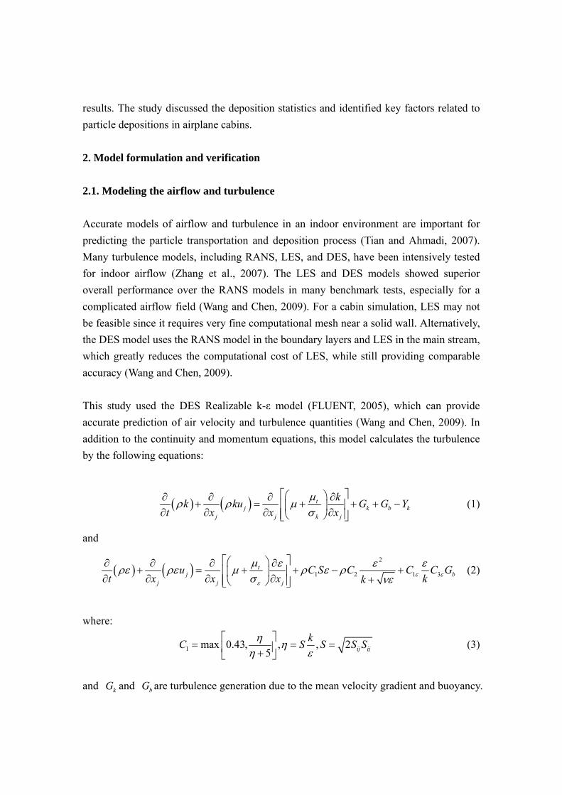
This study used the DES Realizable k-ε model (FLUENT, 2005), which can provide

accurate prediction of air velocity and turbulence quantities (Wang and Chen, 2009). In

addition to the continuity and momentum equations, this model calculates the turbulence

by the following equations:

tj k b k

j j k j

kk ku G G Yt x x x

(1)

and

2

1 2 1 3t

j bj j j

u C S C C C Gt x x x kk

(2)

where:

1 max 0.43, , , 25 ij ij

kC S S S S

(3)

and kG and bG are turbulence generation due to the mean velocity gradient and buoyancy.

1C , 2C , 1C and 2C are constants. The dissipation term in the k equation can be

modeled as: 3/2

kDES

kYl

(4)

where:

min ,DES rke LESl l l (5)

and 3/2

rkekl

(6)

maxLES DESl C (7)

where 0.61DESC is a constant, and max is the maximum local grid spacing

max , ,x y z .

Note that Equation (5) compares the turbulence length scale and the grid spacing. In the

attached boundary layer, the turbulence length scale is smaller than the grid spacing.

Equations (2) and (3) have the same form as the Realizable k-ε model, which calculates

the turbulence kinetic energy and generates the “RANS-like” solution. In the fully

turbulent region, the turbulence length scale is usually larger than the grid spacing.

Equations (2) and (3) become the LES subgrid-scale model, which calculates the

subgrid-scale turbulence kinetic energy and provides a “LES-like” solution.

2.2. Modeling Lagrangian particle motion

With the airflow information, the particle phase can be modeled by both the Eulerian and

Lagrangian methods. The Eulerian method assumes the particle phase to be a continuum

and calculates the particle concentration by solving a scalar transport equation.

Alternatively, the Lagrangian method calculates the motion of a large number of

individual particles and obtains their trajectories. Some studies from the literature have

compared the two methods for particle transportation in an indoor environment (Zhang

and Chen, 2006) and concluded that the Lagrangian method is more accurate and robust,

especially for complex and unsteady airflow cases, which is why the Lagrangian method

was applied in this study.

The Lagrangian method can be expressed as a force balance equation for an individual

particle:

ppD p

p

gduF u u F

dt

(8)

where pu and u are the particle and air velocities, respectively; p and are the

densities of particles and air respectively; g is the gravitational force; F

is other forces

considered in the simulation, including the Thermophoretic force, Saffman lift force, and

Brownian force; and DF is the drag coefficient. Due to the limited space available in

this paper, the formulations of F

and DF are not included, but can be found in the

literature (FLUENT, 2005).

2.3. Modeling particle turbulence dispersion and deposition

Particle deposition occurs within a thin layer near the wall (Lai and Chen, 2006), where

the mean airflow velocity is zero in the wall-normal direction due to the no-slip boundary

condition. However, the turbulence velocity component may not be zero and is a key

factor for particle deposition. Therefore, it is essential to correctly model the turbulence

velocity component, especially near the wall.

In Equation (8), the term u represents the actual airflow velocity, which should be

obtained by solving the airflow models. However, the airflow solution provided by the

DES model may not be sufficient. In the attached boundary layer, where the DES model

switches to RANS mode, the velocity can be written as:

'u u u

(9)

where u is the “RANS-like” mean velocity solved by the DES model, 'u turbulence

velocity component that should be properly modeled.

In the core turbulence region, the DES model switches to LES mode. The air velocity has

the same form as Equation (9) except the term u is the “LES-like” velocity field resolved

by the DES model, and 'u represents the subgrid-scale turbulence fluctuation, which

should also be modeled.

The turbulence dispersion and deposition can be modeled by the Discrete Random Walk

(DRW) model as:

'iζ 2k/3iu (10)

where k is the turbulence kinetic energy in the RANS region and the subgrid-scale

turbulence kinetic energy in the LES region. iζ is a normal random number (FLUENT,

2005).

This model relates the fluctuating air velocity at the particle to the value of the

(subgrid-scale) turbulence kinetic energy in the center of the computational cell in which

the particle is located. This assumption holds if a particle is far from solid walls, where

the variation in turbulence kinetic energy within one cell is negligible. However, in a

wall-adjacent cell, the turbulence kinetic energy decreases to zero all the way from the

cell center to the wall. For a near-wall particle, Equation (10) may overpredict the

fluctuating velocity component, thus causing overprediction of the particle deposition

(Matida et al., 2000).

To correctly predict the fluctuating velocity for the near wall particles, a deposition model

should be applied. Although there is no deposition model available for the DES models,

many models have been developed for different RANS models, which may be used by

the DES in its near wall region. He and Ahmadi (1999) assumed the quadratic variation

of normal Reynolds stress and developed a deposition model for the Reynolds stress

turbulence model. Zhang and Chen (2009) applied the v2f turbulence model and used the

v2 value as the wall normal fluctuation to account for the near wall damping effect. These

two models correctly modeled the near wall behavior and generated a reasonable particle

deposition result. However, these models are only valid for the turbulence models for

which they were developed. For the k-ε family models, Matida et al. (2004) used the

dumping function proposed by Wang and James (1999) for all velocity components. Lai

and Chen (2006) combined the methods of Matida et al. (2004) and He and Ahmadi

(1999) and developed a deposition model with a more concise formulation:

* 2

' 4

42k/3

ii

i

Au y yu

y

(11)

where 0.008A is a constant proposed by Bernard and Wallace (2002), *u is the shear

velocity, and y is the distance from a particle to the nearest wall in the wall unit.

Equation (11) has the same form as Equation (10) if 4y and only applies the

correction in the near wall region. Note that near the wall, this model uses a correlation

instead of the cell center value for the turbulence kinetic energy and thus does not require

a refined near wall mesh. In this study, this model was applied with the DES Realizable

k-ε model to calculate the particle deposition.

2.4. Model verification

This study first validated the DES model with the dispersion and deposition model by

simulating the particle deposition in a cavity with natural convection (Thatcher et al.,

1996). Figure 1 shows the schematic of the cavity, which was a cubic chamber with a

floor and a heated wall, as well as a ceiling and a cooled wall. The front and back walls

were well insulated and adiabatic. This setting generated a counter-clockwise circulation

in the room. Particles of five different sizes were released at the center of the cavity, and

gradually mixed with the air in the cavity. Their deposition was measured at four

differently oriented surfaces.

Figure 1 Schematic and the flow pattern of the inside of the cavity with natural convection (Thatcher et al.

1996).

The numerical simulation was based on ANSYS FLUENT (version 12.1). The

computational mesh contained 262,144 hex cells (64x64x64) with a refined boundary

layer. The DES Realizable k-ε model was applied together with the modified DRW

model.

Figure 2 compares the predicted and measured particle deposition velocity on the four

surfaces. With the DES model, the modified DRW model predicted reasonable results at

the ceiling, floor, and cold wall, but overpredicted the deposition velocity at the warm

wall, which was also found by Zhang and Chen (2009). When used with RANS model

(RNG k-ε), the modified DRW model showed similar performance. Without the near wall

modification, the standard DRW model with DES model overpredicted the deposition

velocity by two orders of magnitude. This was because the near wall grid size was much

larger than the particle size. The turbulence dispersion evaluated at the cell center may be

too large if a particle is close to the wall. In general, the modified DRW model showed

significant improvement over the standard DRW model and will be used in the following

simulation.

Figure 2 Comparison of predicted and measured particle deposition velocity on different surfaces: (a)

ceiling, (b) floor, (c) cool wall, (d) warm wall.

3. Prediction of particle deposition in a four-row airplane cabin

The DES Realizable k-ε model with the modified DRW model has been applied to the

study of the particle deposition in a full-scale four-row cabin mockup. Detailed

experimental data on airflow velocity and particle concentration (Zhang et al., 2009) was

available for further model verification. This study was also modified to study particle

deposition from the breathing and coughing of a passenger.

3.1. Case description

Figure 3 depicts the schematic of the four-row twin-aisle cabin mockup. In the

experiment (Zhang et al., 2009), the cabin mockup had 28 seats, 14 of which were

occupied by human simulators, as shown in red in the figure. The air was supplied from

two groups of linear diffusers located near the center of the ceiling. The total airflow rate

was 0.23 m3/s, or 8.2 L/s per passenger seat. Three-dimensional air velocity and air

temperature were measured at two planes, as depicted in green in Figure 3. The air

velocity and temperature profiles at the inlet diffuser and the temperature of different

surfaces were also measured.

The particle source was located at the center seat of the third row (seat 3D), as shown in

Figure 3. Non-evaporative, monodispersed Di-Ethyl-Hexyl-Sebacat (DEHS) particles

were released from the source into the cabin with a small momentum. After the airflow

and particle field reached a steady-state, the particle concentration was measured at eight

positions, as shown in Figure 3. The particle used in the experiment had a diameter of

0.7μm. However, in the CFD simulation, seven sizes of particles (0.1, 0.7, 2.5, 5, 10, 20,

and 100μm) were simulated to study the influence of particle size on the particle

deposition.

Figure 3 Schematic of the four-row cabin mockup (Zhang et al. 2009).

The numerical simulation was conducted based on CFD code ANSYS FLUENT (version

12.1). The study applied the DES Realizable k-ε model with the modified Lagrangian

method as discussed before. The simulation used a solution from the RNG k-ε model as

the initial field and calculated 10 minutes of flow time to reach the steady-state flow field.

Then, the particles were continuously released from the source into the cabin and were

mixed with the cabin air. For each particle size, 1000 particles were generated every

second. The particle concentration at seats 1A, 1D, 3D and 4D, and the total number of

particles in the cabin were monitored during the calculation. The case was calculated for

another 15 minutes (six complete air changes) of flow time until the particle

concentration field reached steady-state, when the monitored values became stable. The

averaged air velocity, particle concentration, and deposition results were obtained in the

next five minutes of flow time.

3.2. Air velocity and particle concentration field

Figure 4 compares the simulated (DES and RNG k-ε) and measured air velocity vectors

at the cross-section through the third row and at the mid-section along the longitudinal

direction. In the cross-sectional view (Figure 4 (a)), the ceiling diffusers and the thermal

plume in the middle generated two large circulations at each side of the cabin. The DES

prediction agreed with the measurement in terms of circulation pattern. But significant

discrepancies can be found in a quantitative comparison. The result from the RNG k-ε

model was comparable with the DES result, which was also reported by Zhang et al.

(2009), who further concluded that the simulation was very sensitive to the accuracy of

the boundary conditions. In the experiment, the velocity magnitude was accurately

measured, while the direction was not, which generated error for quantitative comparison,

but still preserved qualitative character of the velocity field. Note that the airflow field

was asymmetrical due to the inlet and wall-boundary conditions.

0.3 m/s

(a)

0.3 m/s

(b)

Figure 4 Comparison of simulated (black vectors for DES, and green vectors for RNG k-ε) and measured

(red vectors) airflow field at: (a) the cross-section through the third row, and (b) the mid-section along the

longitudinal direction.

In the mid-section along the longitudinal direction, the vector field shows an upward

motion due to the two circulations and the thermal plume in the middle of the cabin. The

DES result agreed reasonably well with the measured data as shown in Figure 4 (b),

though differences can be found at some positions. For example, at the third row, the DES

model predicted a backward airflow motion, which was not supported by the

measurements. At the same location, the DES results also predicted a smaller upward

velocity than did the experiment. Comparing with the DES model, the RNG k-ε model

predicted larger errors in this section. For such a complex case, a DES model may be

more suitable than the RANS models.

C

Z(m

)

0 1 2 3 4 50

0.5

1

1.5

2

Position 1

C

Z(m

)

0 1 2 3 4 50

0.5

1

1.5

2

Position 2

C

Z(m

)

0 5 10 150

0.5

1

1.5

2

Position 3

C

Z(m

)

0 1 2 3 4 50

0.5

1

1.5

2

Position 4

C

Z(m

)

0 1 2 3 4 50

0.5

1

1.5

2

Position 6

C

Z(m

)

0 1 2 3 4 50

0.5

1

1.5

2

Position 8

C

Z(m

)

0 1 2 3 4 50

0.5

1

1.5

2

Position 7

C

Z(m

)

0 1 2 3 4 50

0.5

1

1.5

2

Position 5

Figure 5 Comparison of the measured (symbols) and predicted (lines) particle concentration profiles in

different positions (C = Clocal/Cexhaust).

Figure 5 compares the simulated and measured concentrations for particles with 0.7 μm

diameter at eight different positions. In general, the DES model predicted reasonably

good results. At position 3 where the source was located, the DES model predicted a

correct shape and magnitude of the concentration peak. However, the peak was slightly

shifted down due to the underpredicted upward velocity. Far from the particle source, the

particle concentration was approximately in a well-mixed condition, which was nicely

captured by the DES model. However at position 8, the DES model overpredicted the

concentration level due to the erroneous backward airflow prediction. For the same

reason, the concentration at position 6 was underpredicted. At position 4, the particle

concentration was underpredicted especially near the ceiling due to the incorrect airflow

prediction closed to the ceiling diffuser. Note that, the predicted concentration profile

shows fluctuation due to the discrete nature of the Lagrangian method, which was also

observed by Zhang et al., (2009). Since the air temperature is not essential for particle

deposition and the space of this paper is limited, this paper did not show validation for the

air temperature. However, good agreement was found between the predicted and

measured air temperature field.

3.3. Particle deposition onto different surfaces

3.3.1. Breathing and talking

In the experiment, the particles were released with a jet flow of velocity magnitude equal

to 1 m/s, which could be representative of the particle release from the breathing (2.5 m/s)

or talking (1.1 m/s) of a passenger (Gupta et al., 2010). The distribution of the particle

deposition at solid walls and exhaust vents was also calculated for five minutes of flow

time in this investigation. The particle deposition density was calculated as:

dA

total

NCN dA

(11)

where dAN was the number of particles deposited on surface area, dA, during a certain

amount of time; totalN was the total number of particles generated during the same time;

and dA was a small surface area, which was the same as the local computational mesh.

This study simulated the particle deposition with seven different particle sizes, which can

be divided into three groups: small particles (0.1, 0.7 and 2.5μm), medium particles (5, 10

and 20μm), and large particles (100μm). Due to the limited space available, this paper

only shows results for the 0.7, 10, and 100 μm particles to represent each category.

Figure 6 shows the particle deposition density of the 0.7, 10, and 100 μm particles. Due

to the asymmetrical airflow pattern, the deposition was also asymmetrical. For the small

(0.7 μm) particles, a high particle deposition density was observed at the ceiling and side

walls along the path of the major circulation (Figure 6(a)), while the floor and seat had

relatively low particle deposition density (Figure 6(d)). This is because the particles were

small and they mainly followed the airflow pattern. The small 0.7 μm particles were

carried by the thermal plume to reach the ceiling, where most particles joined the airflow

circulation formed by the supply jets. The particles deposited at the ceiling and side walls

along their path to the exhaust.

For the medium (10 μm) particles, Figure 6(b) shows that their deposition at the ceiling

and side walls was similar to that of the small particles, but the deposition rate was much

lower. The particle deposition density at the floor was higher. As the particle size

increased, the gravitational force became comparable to the drag force, which changed

the deposition distribution.

For the large (100 μm) particles, Figure 6(c) shows no deposition on the ceiling and side

walls. All the particles were deposited at the surfaces of passenger 3D, as shown in Figure

6(f). For particles of this size, the gravitational force was dominant. The particles had a

free fall motion from its source (mouth/nose) and deposited within a very small area on

passenger 3D.

X

Y

Z

Particle deposition density: 0 0.02 0.04 0.06 0.08 0.1

(a) (b) (c)

(d) (e) (f)

Figure 6 Particle depositions at different surfaces for the breathing and talking case: the top row is for the

ceiling and side wall surfaces and the bottom row for the floor and seats surfaces (a) and (d) for 0.7 μm

particles, (b) and (e) for 10 μm particles, and (c) and (f) for 100 μm particles.

3.3.2. Coughing

This study further modified the initial conditions for the particles so as to study the

particle deposition with a cough from a passenger. As suggested by Gupta et al. (2009),

the coughing jet was injected from the mouth of the passenger 3D with area of opening of

4 cm2, and air velocity of 11.5 m/s. The direction of the jet flow was 22.5 degree

downward along the -y direction. As in the previous case, seven sizes of particles were

continuously released from the cough by the passenger at seat 3D. All the models and

simulation procedures were the same as in the breathing and talking case.

Figure 7(a) shows the particle deposition density of the 0.7 μm particles at the ceiling and

side walls. Compared with the previous case, the deposition on the ceiling and side walls

was significantly reduced. This was because the jet flow that carried the particles could

penetrate the thermal plume. Therefore, most of the particles did not enter the major

circulation so they could not reach the ceiling. For the deposition on the floor and seats,

Figure 7(d) shows a high particle deposition density on the seat back of passenger 2D, the

surface of passenger 3D, and the floor area close to seat 3D, due to the jet impingement.

X

Y

Z

Particle deposition density: 0 0.02 0.04 0.06 0.08 0.1

(a) (b) (c)

(d) (e) (f)

Figure 7 Particle depositions at different surfaces for the coughing case: the top row is for the ceiling and

side wall surfaces and the bottom row is for the floor and seats surfaces (a) and (d) for 0.7 μm particles, (b)

and (e) for 10 μm particles, and (c) and (f) for 100 μm particles.

For the 10 μm particles, Figure 7(b) shows a lower particle deposition density at the

ceiling and side walls than that for the breathing and talking case. As shown in Figure

7(e), a high particle deposition density was observed in the areas of jet impingement.

Unlike the 0.7 μm particles that mostly suspended in the air after entering the air, a

majority of the 10 μm particles deposited due to the jet momentum and the gravity.

For the 100 μm particles, Figure 7(c) shows that no particles deposited on the ceiling and

side walls. All the particles deposited on the back surface of seat 2D, the surface of

passenger 3D, and the floor close to seat 3D due to direct impingement and gravity

because these particles were too heavy to be carried by the airflow.

4. Discussion

The previous section discussed the distribution of particle deposition. For assessing the

infection risk, it is also essential to count the number of particle depositions on different

surfaces, especially at the surfaces in close proximity to the passengers. This

investigation first classified all surfaces into nine categories based on their locations,

properties, and functions. As shown in Figure 8, the nine types of surfaces included:

exhaust, passengers, floor, ceiling, side walls, section ends, seat back, seat front, and tray

tables.

Figure 9 shows the statistics of the particle deposition on different types of surfaces. For

the breathing and talking case (Figure 9 (a)), 65% of the 0.7 μm particles were removed

by air through the exhaust. The side walls and ceiling trapped a large portion of the

particles (12% and 8%, respectively). These surfaces may not be frequently contacted by

passengers. The passenger surfaces had 7% of the 0.7 μm particles. Despite the large area,

the floor only received 3% of the particles. The two section ends trapped 2% of the

particles because the airflow along the longitudinal direction was small. The seat front,

seat back, and tray tables trapped 3% of the particles that could likely be touched by the

passengers. For the 10 μm particles as shown in Figure 9(b), the number of particles

exhausted was reduced to 55%, but was still a majority. The deposition on the ceiling

decreased to 2% since gravity became important for this size of particle. For the 100 μm

particle as shown in Figure 9(c), 100% of the particles deposited on the surface of the

index passenger, which can be explained by their free fall motion. In general, the gravity

force played a major role in the particle deposition.

 

Figure 8 Definitions of the nine different types of surfaces.

Figure 9 Statistics of particle deposition on different types of surfaces: (a) 0.7 μm particles in the breathing

case, (b) 10 μm particles in the breathing case, (c) 100 μm particles in the breathing case, (d) 0.7 μm

particles in the coughing case, (e) 10 μm particles in the coughing case, and (f) 100 μm particles in the

coughing case.

In the coughing case, the jet could penetrate the thermal plumes and could transport the

particles to the lower part of the cabin. The jet impingement enhanced particle deposition

on the floor, thus increasing the total particle deposition by 13% and 14% for the 0.7 μm

and the 10 μm particles, respectively, as shown in Figures 9(d) and 9(e). For the two

particle sizes, the deposition on the passenger also increased. The deposition on the

ceiling and side walls decreased slightly. As shown in Figure 9(f), 91% of the 100 μm

particles deposited on the floor, with the rest on the seat back and tray table in front of the

index passenger.

5. Conclusion

This study applied the DES model with a modified Lagrangian method to predict the

particle dispersion in a cavity with natural convection and in a four-row airplane cabin

mockup. By comparing with the experimental data, this investigation found that this new

model can predict reasonably good results for air velocity, particle concentration, and

particle deposition for the two cases.

For the cabin case, seven sizes of particles were assumed to be released by an index

passenger sitting in the middle of the cabin due to breathing with zero velocity and due to

coughing with suitable jet velocity. This study found that the distribution of particle

deposition onto surfaces depended on particle size, particle release mode, and the airflow

pattern in the cabin. In the breathing case, 35% of the small (0.7μm) particles, 55% of the

medium (10μm) particles, and 100% of the large (100μm) particles deposited onto the

cabin surface and the rest were removed by the cabin ventilation. In the coughing case,

the number of small, medium and large particles particles deposited changed to 48%,

69%, and 100%, respectively.

References

ACI. The Global Airport Community, 2007. www.airports.org/aci/aci/file/Annual

Report/ACI Annual Report 2006 FINAL.pdf

Baker, A. J., Ericson S.C., Orzechowski, J.A., Wong K.L. and Garner, R.P., 2006. Aircraft

passenger cabin ECS-generated ventilation velocity and mass transport CFD

simulation: Velocity field validation. Journal of the IEST (Online) 49(2), 51-83.

Baker, A. J., Ericson S.C., Orzechowski, J.A., Wong, K.L. and Garner, R.P., 2008.

Aircraft passenger cabin ECS-generated ventilation velocity and mass transport CFD

simulation: Mass transport validation exercise. Journal of the IEST (Online) 51(1),

90-113.

Bernard, P. S., and Wallace, J. M., 2002. Turbulent flow: Analysis, measurement and

prediction, New Jersey: Wiley.

Chen, Q., 2008. Ventilation performance prediction for buildings: A method overview and

recent applications. Building and Environment 44(4), 848-58.

FLUENT, 2005. Fluent 6.2 Documentation. Fluent Inc., Lebanon, NH.

Gunther, G., Bosbach, J., Pennecot, J., Wagner, C., Lerche, T. and Gores, I., 2006.

Experimental and numerical simulations of idealized aircraft cabin flows. Aerospace

Science and Technology 10(7), 563-573.

Gupta, J.K., Lin, C.-H. and Chen, Q., 2009. Flow dynamics and characterization of a

cough. Indoor Air 19, 517-525.

Gupta, J.K., Lin, C.-H., and Chen, Q., 2010. Characterizing exhaled airflow from

breathing and talking. Indoor Air 20, 31-39.

He, C. and Ahmadi, G., 1999. Particle deposition in a nearly developed turbulent duct

flow with electrophoresis. Journal of Aerosol Science 30, 739-758.

Lai, A. C. K. and Nazaroff, W.W., 2000. Modeling indoor particle deposition from

turbulent flow onto smooth surfaces. Journal of Aerosol Science 31, 463-476.

Lai A. C. K. and Chen F., 2006. Modeling of particle deposition and distribution in a

chamber with a two-equation Reynolds-averaged Navier–Stokes model. Journal of

Aerosol Science 37(12), 1770-80.

Mangili, A. and Gendreau, M.A., 2005. Transmission of infectious diseases during

commercial air travel. Lancet 365, 989-996.

Matida, E. A., Nishino, K. and Torii, K., 2000. Statistical simulation of particle deposition

on the wall from turbulent dispersed pipe flow. International Journal of Heat and

Fluid Flow 21, 389-402.

Matida, E. A., Finlay, W. H., Lange, C. F. and Grgic, B., 2004. Improved numerical

simulation of aerosol deposition in an idealized mouth–throat. Journal of Aerosol

Science 35, 1-19.

Poussou, S., Mazumdar, S., Plesniak, M.W., Sojka, P. and Chen, Q., 2010. Flow and

contaminant transport in an airliner cabin induced by a moving body: Scale model

experiments and CFD predictions. Atmospheric Environment 44(24), 2830-2839.

Spalart, P. R. and Bogue, D. R., 2003. The role of CFD in aerodynamics, off-design.

Aeronautical Journal 107(1072), 323-329.

Spengler, J. D. and Wilson, D. G.., 2003. Air Quality in Aircraft, Proceedings of the

Institution of Mechanical Engineers, Part E: Journal of Process Mechanical

Engineering 217, 323-335.

Thatcher, T.L., Fairchild, W.A. and Nazaroff, W.W., 1996. Particle deposition from

natural convection enclosure flow onto smooth surfaces. Aerosol Science and

Technology 25, 359-374.

Tian, L. and Ahmadi, G., 2007. Particle deposition in turbulent duct flows - comparisons

of different model predictions. Journal of Aerosol Science 38, 377-397.

Wang, M. and Chen, Q., 2009. Assessment of various turbulence models for transitional

flows in enclosed environment, HVAC&R Research 15(6), 1099-1119.

Wang, Y. and James, P. W., 1999. On the effect of anisotropy on the turbulent dispersion

and deposition of small particles. International Journal of Multiphase Flow 5,

551-558.

Zhang, Z. and Chen, Q., 2006. Experimental measurements and numerical simulations of

particle transport and distribution in ventilated rooms. Atmospheric Environment

40(18), 3396-3408.

Zhang Z, Zhai ZQ, Zhang W, Chen Q., 2007. Evaluation of various turbulence models in

predicting airflow and turbulence in enclosed environments by CFD: Part

2-comparison with experimental data from literature. HVAC&R Research

13(6):871-886.

Zhang, Z. and Chen, Q., 2009. Prediction of particle deposition onto indoor surfaces by

CFD with a modified Lagrangian method. Atmospheric Environment 43(2),

319-328.

Zhang, Z., Chen, X., Mazumdar, S., Zhang, T. and Chen, Q., 2009. Experimental and

numerical investigation of airflow and contaminant transport in an airliner cabin

mockup. Building and Environment 44(1), 85-94.

Zhao B., Yang C., Yang X. and Liu S., 2008. Particle dispersion and deposition in

ventilated rooms: Testing and evaluation of different Eulerian and Lagrangian

models. Building and Environment 43(4), 388-97.