Determination of Parameters of EVP Material Model in ... · Determination of Parameters of EVP...

Determination of Parameters of EVP Material Model in Numerical Welding Simulations

JOSEF BRADÁČ

Department of Automobile Technology Škoda Auto University

V. Klementa 869, Mladá Boleslav CZECH REPUBLIC [email protected]

Abstract: Numerical simulations are used more and more frequently in technological processes, including welding processes. They are used especially for the selection of the right welding procedure, prediction and analysis of resulting deformations and distortions and also for the resulting structure of the weld metal. Size and placement determination of the residual inner stresses in the material after welding are equally important, mainly in reference to the capacity and stability of the welded structures and the prediction of their behavior during different types of load. The submission deals with determination of parameters of EVP (elastic viscoplastic) material model, by help of these parameters it is possible to describe more precisely the residual stresses during and after the welding process. In comparison with commonly used constitutive models, the advantage of this model is that it also covers viscoplastic processes, which in reality take place by stress relaxation at high temperatures. Key-Words: EVP material model, numerical simulations, viscoplastic processes, relaxation, Sysweld program 1 Introduction Dynamical development of information technologies in the last few years has also lead to the progress in numerical simulations. These programs work mainly on the basis of the finite element method. Thanks to that it is then possible to solve more complex tasks while shorter computation times. The Sysweld simulation program from French company ESI also has these mentioned advantages and belongs to the most sophisticated programs for fusion welding and heat treatment [2]. The actual computation in this program is divided into two stages: thermal-metallurgic analysis and mechanical analysis.

The thermal-metallurgical analysis solves the computation of non-stationary temperature fields, phase transformation, hardness of the structure, and of the austenitic grain size, as appropriate. This is quadrated with the material input data, which should be entered in a temperature dependent form [1]. The mechanical analysis follows the thermal-metallurgical analysis and it is not possible to carry it out without a previous thermal load of the scale. It enables to compute a time curve of the individual stress tensor factors, main stress values, spatial stress-strain state according to the HMH theory, as well as the shear stress Tresc analysis. The computation of elastic and plastic deformation of

the individual components as well as of the residual stress tensor is also possible [4,20].

In current time two constitutive models for computation of residual stresses after welding are used. The first one is the elastic-plastic material model with isotropic hardening and the second one is the elastoplastic material model with kinematic hardening. In general by using the elastoplastic material model with isotropic hardening, the values of residual stresses are higher comparing to the elastoplastic material model with kinematic hardening [8]. However the real welding process involves relaxation of stresses due to high temperatures, meaning that the real values of residual stresses are lower than both of the elastoplastic material models show [7]. The reason is that elastoplastic material model is not, by its own physical virtue, able to reflect the viscoplastic processes, which in reality proceed during the stress relaxation. The submission aims to explain the methodology of determination of parameters of EVP material model of steel X5CrNi1810 and the way of entering the determined data into the computation module in the Sysweld simulation program.

WSEAS TRANSACTIONS on APPLIED and THEORETICAL MECHANICS Josef Bradáč

E-ISSN: 2224-3429 202 Issue 3, Volume 8, July 2013

2 Numerical Simulations in Sysweld program Sysweld is a program which is based on final element method (FEM). This approach has been developed to cover the need for broad shape variability and to satisfy a demand for individual solutions in the case of single subgroups of special model. That‘s why it is possible in this case to use any shape of individual elements as opposed to the final difference method (FDM). This access arisen reason was to requirement of high shape variability and needs to solve individual subgroups of solid model separately [6]. That is the reason why it is there possible to use random shape of individual elements, comparing in case to finite difference method. From mathematical point of view it is possible to use the finite element method for finding the approximated solutions for partial differential and integral formulas, e.g. for the heat conduction formula [3].

The overall process is divided according to the SYSWELD program into the two basic parts, the thermo-metallurgical part and the mechanical part. 2.1 Thermo-metallurgical analysis The thermo-metallurgical analysis enables the calculations of the temperature field for given space and time, the calculation and the depiction of phase structures during the overall welding cycle and during the cooling off period. It enables to calculate the structural hardness and the size of austenitic grain.

This is quadrated with the material input data, which should be entered in a temperature dependent form. The thermal-metallurgical analysis input data are [14]:

- chemical composition, - CCT transformation diagram, only with

materials which undergo a phase transformation,

- temperature dependence of specific heat conductivity λ,

- temperature dependence of specific heat c, - temperature dependence of density ρ, - temperature dependence of heat transfer

coefficient β. 2.2 Mechanical analysis The mechanical analysis is based on the thermo-metallurgical analysis and it cannot be done without

previous heating of a system. The program enables to define the time evolution for elasticity and plasticity deformations and relative and absolute values for individual nodes points shifting. The program can above all calculate the deformation energy density. The mechanical analysis input data are [16,19]:

- Temperature dependence of Poisson´s ratio µ,

- Temperature dependence of Young’s modulus (modulus of elasticity) E,

- Temperature dependence of distensibility coefficient α,

- Temperature dependence of Yeld strength Re,

- Temperature dependence of material strain hardening H,

- Input values for viscoplastic material behavior.

2.3 Output data presentation possibilities Each shape model is deposit of elements and nodes points. Whole model is divided to several zones, whereas several element sizes are from district to district different. That’s why element density is based on element size in given district is different. District with high node points density are there, where we can get more detailed informations, e.g. weld metal district, heating affected zone, fixation places of weld parts, see figure 1.

Fig. 1 Shape model of butt weld

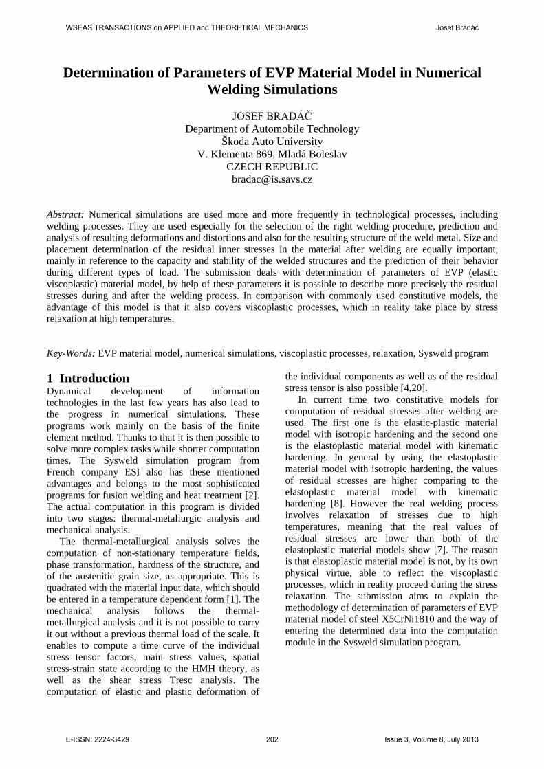
On the figure 2 we can see part of model which

is composited of elements and node points. Node points are in green and elements in red color. Simplified say, we can computed data presented



either by elements, or by node points, whereas computed results presentation can slip in graphical form or data files.

The basic difference between element and node point is at that, that element or element group represent quantity always in one computed time. So for disposal chosen time is by graphical form of commutations presentation, see the interval of depict quantity values [2,3].

Fig. 2 Part of model composited of elements and node points

So in the case of diagram computation

presentation we can see the interval of values of presented quantity for the selected time. On the figure 3 there is a graphical depiction of quantity scheme (in our case temperature) on the surface of weld model hand made using the method 141 at the time t=50s, where the heat source is in the middle of weldment.

Fig. 3 Temperature field on the butt weld shape model

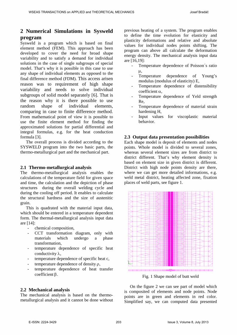
The node point, which is the boundary point of the element on the contrary, depicts only time dependence of presented quantity. It means, that for one computed time we get only one examined quantity value. On the figure 4 we can see time dependence of presented value (temperature) in graphical form for selected node points in heat affected zone [17,18].

Fig. 4 Temperature-time dependence scheme for selected node points

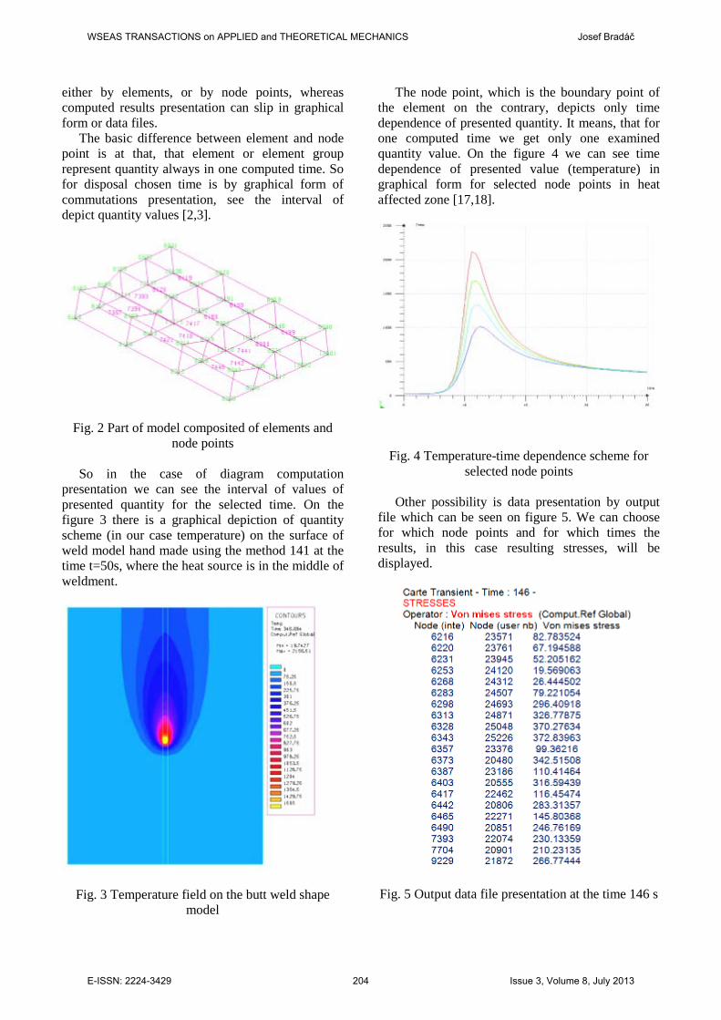
Other possibility is data presentation by output

file which can be seen on figure 5. We can choose for which node points and for which times the results, in this case resulting stresses, will be displayed.

Fig. 5 Output data file presentation at the time 146 s



2.3 Output data fault Although we can obtain many important and usable data from thermal metallurgical and mechanical analysis and even that it is possible to use such data in order to explore in detail any zone of shape model, this program does not solve the issue of critical places analyses.

Although it is possible to focus on the zones with high stresses and then solve the issues of these zones by detailed analysis of individual node points, this procedure is at first rather complicated and time consuming and at second maximal stresses areas can change during welding and consequent cooling and do change indeed. It means, that for detailed numerical weld analyses examination, we should examine the areas with maximal stresses in each defined time and in parallel also examine temperature at given point and time, because all mechanical properties used for comparative analysis are temperature dependent [5]. That is the reason why we cannot come to the conclusion, that the site of maximal stresses must be also the critical place for crack creation. For us, the critical places are these where the spatial stress reaches or overreaches the strength limit of the material for given temperature. Unfortunately the program Sysweld as well as other simulations programs conversant with welding technology cannot detect such places [1].

Next element of high importance is the size of plastic deformation. If we consider only the resulting stress state at given time, which is even much lower than the strength limit for given temperature, it does not mean that we have reached the correct result. The way of how we reached this stress value is of relevance as well. It gives answers to the question whether the plasticity has been already exhausted due to the tensile and compressive stress changes.

3 Material Behavior Patterns When solving tasks related to plastic deformation we cannot manage only with two constants that characterize material behavior in the linear elasticity theory. On the contrary it is important to know characteristics ( )εσσ = under given conditions, i.e. temperature, stress rate as well as the size and shape of the solid. Very slow processes, when ε < 1510 −− s by constant force effects, .const=σ cause deformation dependent on time [13]. This deformation is known as viscous and the process is known as creep process. In the range of deformation

124 10,10 −−−∈ sε the viscous transformation does

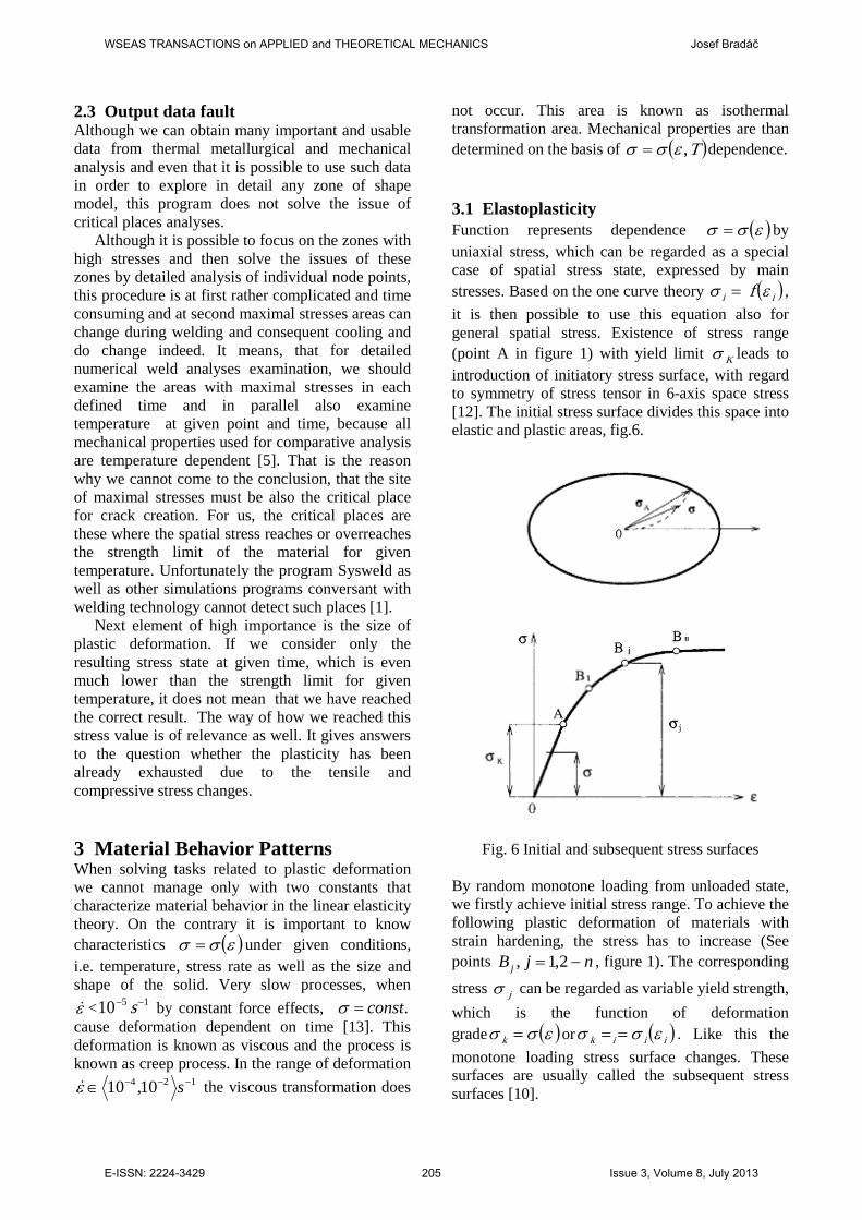
not occur. This area is known as isothermal transformation area. Mechanical properties are than determined on the basis of ( )T,εσσ = dependence. 3.1 Elastoplasticity Function represents dependence ( )εσσ = by uniaxial stress, which can be regarded as a special case of spatial stress state, expressed by main stresses. Based on the one curve theory ( )ii f εσ = , it is then possible to use this equation also for general spatial stress. Existence of stress range (point A in figure 1) with yield limit Kσ leads to introduction of initiatory stress surface, with regard to symmetry of stress tensor in 6-axis space stress [12]. The initial stress surface divides this space into elastic and plastic areas, fig.6.

Fig. 6 Initial and subsequent stress surfaces

By random monotone loading from unloaded state, we firstly achieve initial stress range. To achieve the following plastic deformation of materials with strain hardening, the stress has to increase (See points njBj −= 2,1, , figure 1). The corresponding

stress jσ can be regarded as variable yield strength, which is the function of deformation grade ( )εσσ =k or ( )iiik εσσ == . Like this the monotone loading stress surface changes. These surfaces are usually called the subsequent stress surfaces [10].



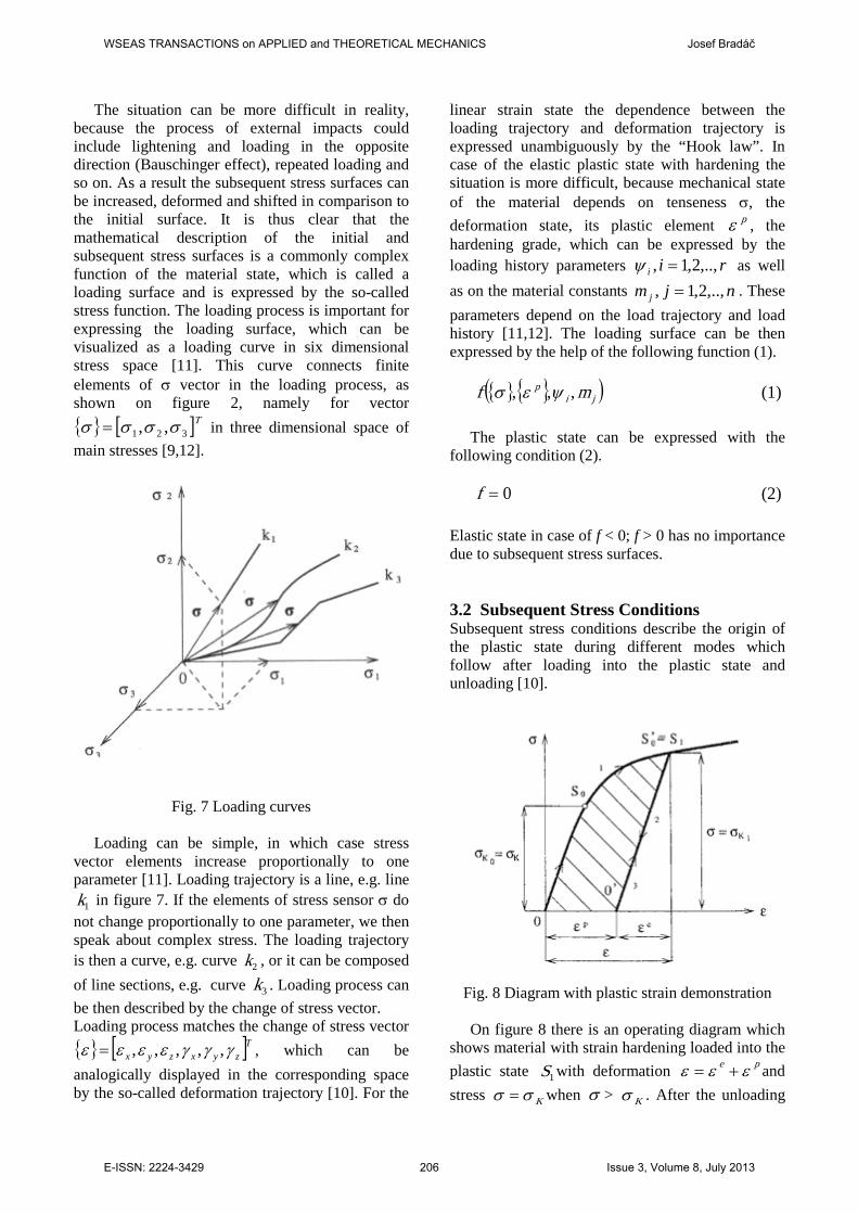
The situation can be more difficult in reality, because the process of external impacts could include lightening and loading in the opposite direction (Bauschinger effect), repeated loading and so on. As a result the subsequent stress surfaces can be increased, deformed and shifted in comparison to the initial surface. It is thus clear that the mathematical description of the initial and subsequent stress surfaces is a commonly complex function of the material state, which is called a loading surface and is expressed by the so-called stress function. The loading process is important for expressing the loading surface, which can be visualized as a loading curve in six dimensional stress space [11]. This curve connects finite elements of σ vector in the loading process, as shown on figure 2, namely for vector { } [ ]T321 ,, σσσσ = in three dimensional space of main stresses [9,12].

Fig. 7 Loading curves

Loading can be simple, in which case stress vector elements increase proportionally to one parameter [11]. Loading trajectory is a line, e.g. line

1k in figure 7. If the elements of stress sensor σ do not change proportionally to one parameter, we then speak about complex stress. The loading trajectory is then a curve, e.g. curve 2k , or it can be composed of line sections, e.g. curve 3k . Loading process can be then described by the change of stress vector. Loading process matches the change of stress vector { } [ ]Tzyxzyx γγγεεεε ,,,,,= , which can be analogically displayed in the corresponding space by the so-called deformation trajectory [10]. For the

linear strain state the dependence between the loading trajectory and deformation trajectory is expressed unambiguously by the “Hook law”. In case of the elastic plastic state with hardening the situation is more difficult, because mechanical state of the material depends on tenseness σ, the deformation state, its plastic element pε , the hardening grade, which can be expressed by the loading history parameters rii ,..,2,1, =ψ as well as on the material constants njm j ,..,2,1, = . These parameters depend on the load trajectory and load history [11,12]. The loading surface can be then expressed by the help of the following function (1).

{ } { }( )ji

p mf ,,, ψεσ (1) The plastic state can be expressed with the

following condition (2).

0=f (2)

Elastic state in case of f < 0; f > 0 has no importance due to subsequent stress surfaces. 3.2 Subsequent Stress Conditions Subsequent stress conditions describe the origin of the plastic state during different modes which follow after loading into the plastic state and unloading [10].

Fig. 8 Diagram with plastic strain demonstration

On figure 8 there is an operating diagram which shows material with strain hardening loaded into the plastic state 1S with deformation pe εεε += and stress Kσσ = when σ > Kσ . After the unloading



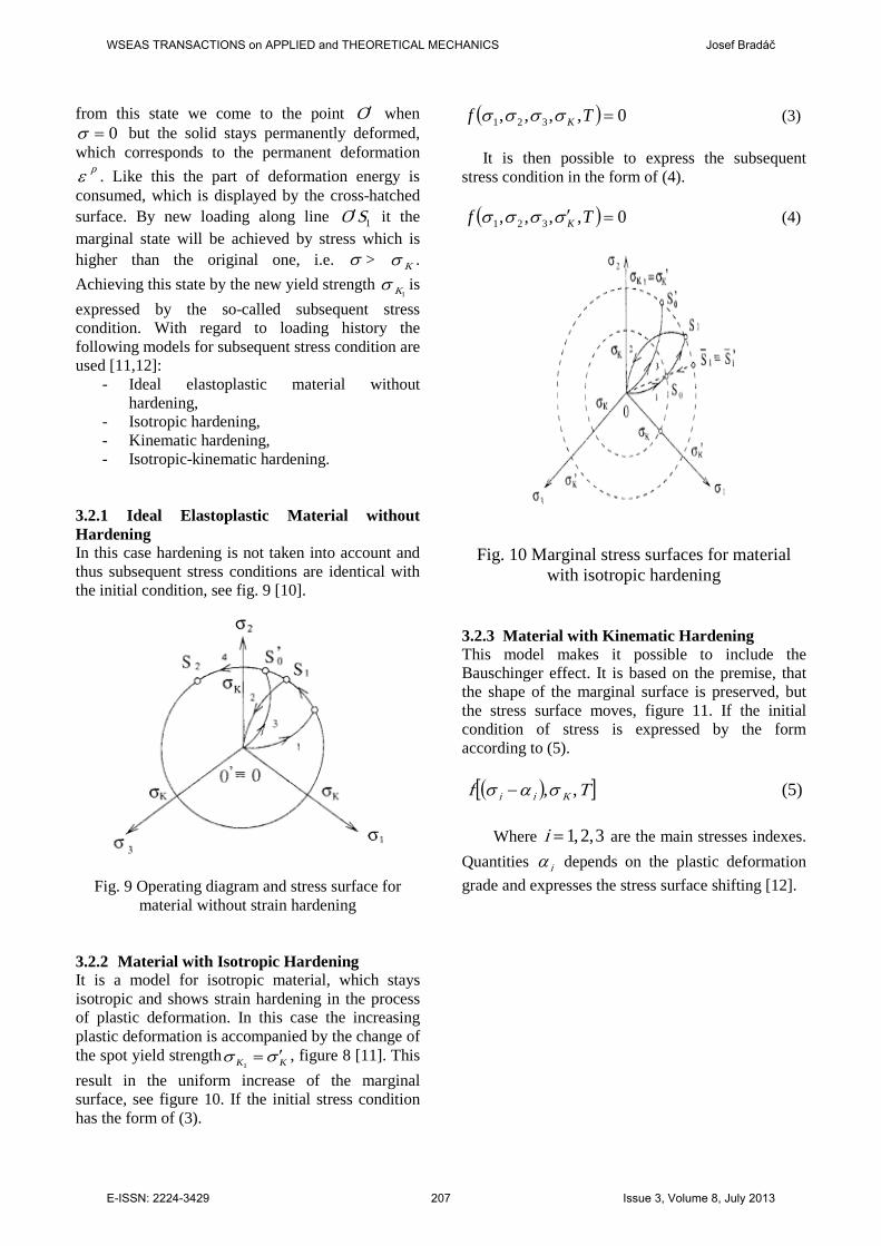
from this state we come to the point O′ when 0=σ but the solid stays permanently deformed,

which corresponds to the permanent deformation pε . Like this the part of deformation energy is

consumed, which is displayed by the cross-hatched surface. By new loading along line 1SO′ it the marginal state will be achieved by stress which is higher than the original one, i.e. σ > Kσ . Achieving this state by the new yield strength

1Kσ is expressed by the so-called subsequent stress condition. With regard to loading history the following models for subsequent stress condition are used [11,12]:

- Ideal elastoplastic material without hardening,

- Isotropic hardening, - Kinematic hardening, - Isotropic-kinematic hardening.

3.2.1 Ideal Elastoplastic Material without Hardening In this case hardening is not taken into account and thus subsequent stress conditions are identical with the initial condition, see fig. 9 [10].

Fig. 9 Operating diagram and stress surface for material without strain hardening

3.2.2 Material with Isotropic Hardening It is a model for isotropic material, which stays isotropic and shows strain hardening in the process of plastic deformation. In this case the increasing plastic deformation is accompanied by the change of the spot yield strength KK σσ ′=

1, figure 8 [11]. This

result in the uniform increase of the marginal surface, see figure 10. If the initial stress condition has the form of (3).

( ) 0,,,, 321 =Tf Kσσσσ (3)

It is then possible to express the subsequent stress condition in the form of (4). ( ) 0,,,, 321 =′ Tf Kσσσσ (4)

Fig. 10 Marginal stress surfaces for material with isotropic hardening

3.2.3 Material with Kinematic Hardening This model makes it possible to include the Bauschinger effect. It is based on the premise, that the shape of the marginal surface is preserved, but the stress surface moves, figure 11. If the initial condition of stress is expressed by the form according to (5).

( )[ ]Tf Kii ,,σασ − (5)

Where 3,2,1=i are the main stresses indexes. Quantities iα depends on the plastic deformation grade and expresses the stress surface shifting [12].



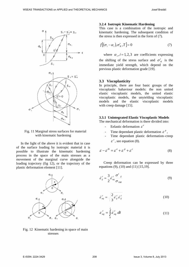
Fig. 11 Marginal stress surfaces for material with kinematic hardening

In the light of the above it is evident that in case

of the surface loading by isotropic material it is possible to illustrate the kinematic hardening process in the space of the main stresses as a movement of the marginal curve alongside the loading trajectory (fig 12), or the trajectory of the plastic deformation element [11].

Fig. 12 Kinematic hardening in space of main stresses

3.2.4 Isotropic Kinematic Hardening This case is a combination of the isotropic and kinematic hardening. The subsequent condition of the stress is then expressed in the form of (7).

( )[ ] 0,, =′− Tf Kii σασ (7)

where 3,2,1, =iiα are coefficients expressing the shifting of the stress surface and Kσ ′ is the immediate yield strength, which depend on the previous plastic deformation grade [19].

3.3 Viscoplasticity In principle, there are four basic groups of the viscoplastic bahaviour models: the non united elastic viscoplastic models, the united elastic viscoplastic models, the unyielding viscoplastic models and the elastic viscoplastic models with creep damage [15]. 3.3.1 Unintegrated Elastic Viscoplastic Models The mechanical deformation is there divided into:

- Eelastic deformation eε - Time dependant plastic deformation pε , - Time dependant plastic deformation–creep

cε , see equation (8).

cpeth εεεεε ++=− (8)

Creep deformation can be expressed by three equations (9), (10) and (11) [15,19].

VM

ijceq

cij σ

σεε

′=

23 (9)

cij

cij

ceq εεε

32

= (10)

∫=t

ceq

ceq dt

0

εε (11)



3.3.2 United Elastic Viscoplastic Models Compared to the previous model, this model uses only one plastic deformation in its computation, which is the viscoplastic deformation pε (12).

thpe εεεε ++= (12)

This model counts on the existence of the elasticity area, inside which the reversible elastic deformation occurs only for a short period of time. This area is defined on the basis of the scalar value of function F, see (13).

( ) 0,, ≤= peqijijFF εχσ (13)

Function F depends on the transformation state.

Inner changes reflect the material yield strength. As in the case of elastic-plasticity we can distinguish between two types of strain hardening, and thus isotropic, kinematic or their combination [11,15].

3.3.3 Universal Elastic Viscoplastic Model The mathematical and physical principle of the universal elastic viscoplastic (EVP) material model is given by the following equations (14) and (15) [3,15].

( )

i

i

N

Meffii

yi

eqieq

i

K

−

= 1

ε

σσε (14)

( ) ( ) 0/1/1=−−= ii Neq

iMeff

iiyi

eqii Kf εεσσ (15)

Where

•eqiε is viscoplastic deformation rate

corresponds to the parallel phase, eqiσ is reduced

stress effiε is scalar parameter of the actual

viscoplastic deformation, yiσ is relaxation stress and

iK , iM , iN are parameters which express viscoplastic behaviour of the material [3]. 4 Determination of EVP Material Model Parameters This section briefly describes the procedure of the determination of parameters of the EVP material

model for stainless steel X5CrNi1810. The elastic viscoplastic material model, which takes into account relaxation procedures in the material during and after the welding process, is described by four parameters [7].

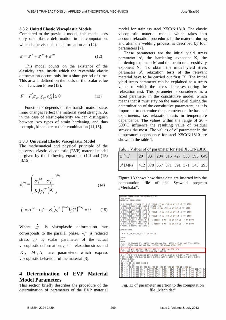
These parameters are the initial yield stress parameter σy, the hardening exponent K, the hardening exponent M and the strain rate sensitivity exponent N. To obtain the initial yield stress parameter σy, relaxation tests of the relevant material have to be carried out first [3]. The initial yield stress parameter can be explained as a stress value, to which the stress decreases during the relaxation test. This parameter is considered as a fixed parameter in the constitutive model, which means that it must stay on the same level during the determination of the constitutive parameters, as it is important to determine the parameter on the basis of experiments, i.e. relaxation tests in temperature dependence. The values within the range of 20 - 500°C influence the resulting value of residual stresses the most. The values of σy parameter in the temperature dependence for steel X5CrNi1810 are shown in the table 1.

Tab. 1 Values of σy parameter for steel X5CrNi1810

T [°C] 20 93 204 316 427 538 593 649

σy [MPa] 412 378 357 371 391 371 343 295

Figure 13 shows how these data are inserted into the computation file of the Sysweld program „Mech.dat“.

Fig. 13 σy parameter insertion to the computation file „Mech.dat“



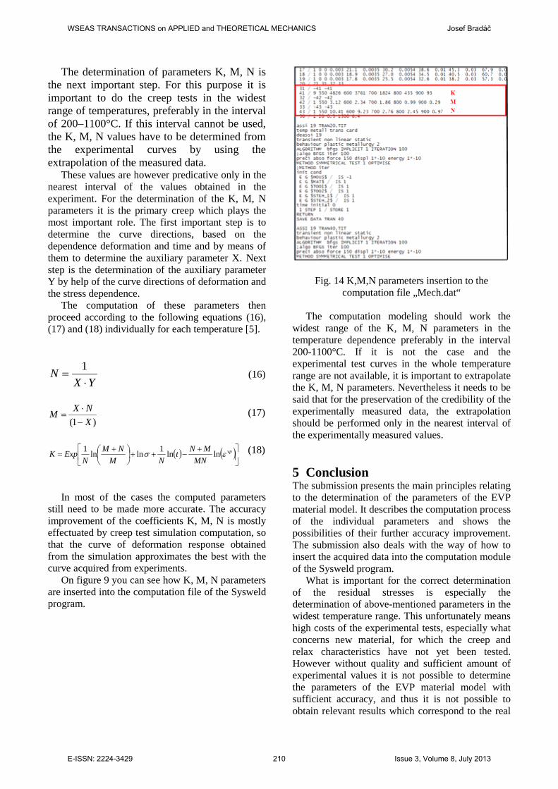
The determination of parameters K, M, N is the next important step. For this purpose it is important to do the creep tests in the widest range of temperatures, preferably in the interval of 200–1100°C. If this interval cannot be used, the K, M, N values have to be determined from the experimental curves by using the extrapolation of the measured data.

These values are however predicative only in the nearest interval of the values obtained in the experiment. For the determination of the K, M, N parameters it is the primary creep which plays the most important role. The first important step is to determine the curve directions, based on the dependence deformation and time and by means of them to determine the auxiliary parameter X. Next step is the determination of the auxiliary parameter Y by help of the curve directions of deformation and the stress dependence.

The computation of these parameters then proceed according to the following equations (16), (17) and (18) individually for each temperature [5].

YXN

⋅=

1 (16)

)1( XNXM

−⋅

= (17)

( ) ( )

+−++

+

= vp

MNMNt

NMNM

NExpK εσ lnln1lnln1 (18)

In most of the cases the computed parameters

still need to be made more accurate. The accuracy improvement of the coefficients K, M, N is mostly effectuated by creep test simulation computation, so that the curve of deformation response obtained from the simulation approximates the best with the curve acquired from experiments.

On figure 9 you can see how K, M, N parameters are inserted into the computation file of the Sysweld program.

Fig. 14 K,M,N parameters insertion to the computation file „Mech.dat“

The computation modeling should work the

widest range of the K, M, N parameters in the temperature dependence preferably in the interval 200-1100°C. If it is not the case and the experimental test curves in the whole temperature range are not available, it is important to extrapolate the K, M, N parameters. Nevertheless it needs to be said that for the preservation of the credibility of the experimentally measured data, the extrapolation should be performed only in the nearest interval of the experimentally measured values.

5 Conclusion The submission presents the main principles relating to the determination of the parameters of the EVP material model. It describes the computation process of the individual parameters and shows the possibilities of their further accuracy improvement. The submission also deals with the way of how to insert the acquired data into the computation module of the Sysweld program.

What is important for the correct determination of the residual stresses is especially the determination of above-mentioned parameters in the widest temperature range. This unfortunately means high costs of the experimental tests, especially what concerns new material, for which the creep and relax characteristics have not yet been tested. However without quality and sufficient amount of experimental values it is not possible to determine the parameters of the EVP material model with sufficient accuracy, and thus it is not possible to obtain relevant results which correspond to the real



state of the residual stresses in the material after welding. From these reasons it is recommended to verify the computed residual stresses with the EVP material model by means of a suitable experimental method, and thus also the credibility of the computed results. References: [1] Moravec, J., Bradáč, J., Selection of Right

Technological welding Procedure on the Simulations Computations Basis, New Findings in Technologies, 2008, ISBN 978-80-7044-969-1.

[2] Bradáč J., Using Welding Simulations to Predict Deformations and Distortions of Complex Car Body Parts with more Welds, Machines, Technologies, Materials, vol. VII, No. 1/12, 2013, ISSN 1313-0226.

[3] Wen, S.W., Finite Element Modelling of Residual Stress and Distortion in SAW Weld, Swinden Technology Centre England, 2004.

[4] Souloumiac, B., Boitout, F., Bergheau, J.M., New Local-Global Approach for the Modeling of Welded Steel Component Distortions, International Scientific Union, 2004.

[5] Radaj, D., Welding Residual Stresses and Distortion - Calculation and Measurement, DVS Verlag, 2003.

[6] Miakami, Y., Morikage, Y., Mochizuki, M., Toyoda, M., Welding Distortion through Numerical Simulation Considering Phase Transformation Effect, International Institute of Welding, 2005.

[7] Yanagida, N., Residual Stress Improvement in Multi-Layer Welding of Austenitic Stainless Steel Plates Using Water-Shower Cooling During Welding Process, International Institute of Welding, 2006.

[8] Li, J., Localized Thermal Tensioning Technique to Prevent Buckling Distortion, Welding in The World, vol. 49, No. 11/12, 2005, ISSN 0043-2288.

[9] Ogden, R.W., Nonlinear Elastic Deformations, Dover Publications, 1997.

[10] Chaboche, J.L., Time-Independent Constitutive Theories for Cyclic Plasticity, International Journal of Plasticity, Vol. 2, No 2, 1986, ISSN 0749-6419.

[11] Kachanov, L.M., Foundations of the Theory of Plasticity, North-Holland Publishing, 1971.

[12] Plánička, F., Kuliš, Z., Stress Theory, ČVUT Prague, 2004.

[13] Sysweld Program Reference Manual, Isotropic Linear Elasticity, ESI Group, 2006.

[14] Sysweld Program Reference Manual, Anisotropic Linear Elasticity, ESI Group, 2006.

[15] Sysweld Program Reference Manual, Viscoplasticity, ESI Group, 2006.

[16] Sysweld Program Reference Manual, Metallurgical Transformation Model, ESI Group, 2006.

[17] Sysweld Program Reference Manual, Heat Input Fitting Module, ESI Group, 2006.

[18] Sysweld Program Reference Manual, Heat exchange and welding heat source, ESI Group, 2006.

[19] Sysweld Program Reference Manual, Numerical Determination of Hardness, ESI Group, 2006.

[20] Sysweld Program Reference Manual, Hardness Analysis Module, ESI Group, 2006.



Determination of Parameters of EVP Material Model in ... · Determination of Parameters of EVP...

Documents

Transcript of Determination of Parameters of EVP Material Model in ... · Determination of Parameters of EVP...