The cost of assuming a lateral density distribution in corrections to Helmert orthometric heights
International Journal of Electronics,
Communication & Instrumentation Engineering
Research and Development (IJECIERD)
ISSN(P): 2249-684X; ISSN(E): 2249-7951
Vol. 4, Issue 1, Feb 2014, 123-134
© TJPRC Pvt. Ltd.
DETERMINATION OF ORTHOMETRIC HEIGHTS FROM GPS AND LEVELLING DATA
EDAN J. D, IDOWU, T. O, ABUBAKAR T & ALIYU, M. R
Department of Surveying & Geoinformatics, Modibbo Adama University of Technology,
Yola, Adamawa State, Nigeria
ABSTRACT
One of the major tasks of geodesy is the determination of geoid. This task is getting more crucial due to the
development of global positioning systems (GPS). This is due to the fact that GPS provide ellipsoidal heights instead of
orthometric heghts. To convert ellipsoidal heights into orthometric heights, precise geoid heights are required. Nowadays,
the most effective universal technique used for the determination of orthometric heights is the GPS and Levelling
technique. This paper focuses on this technique and multiple regression analysis method was used to further determine the
geoid undulations .ArcGIS 9.2 software was used for generating the grid map of the area using the corrected orthometric
heights obtained by the regression method.
The regression parameters a0, x1 and x2 were obtained as 1166.721268, -0.00085137265 and -0.00089422771399
respectively. From the analysis, the standard error of estimates Sϰ1 and Sϰ2 associated with x1 and x2 were obtained as
0.0001291688765 and 0.0001351270512 respectively. The coefficient of multiple determination R2 was found to be
0.992049442. the computed F-statistic was 5157.59101, while the value from F-distribution table was 3.97. Hence, the
parameter estimators ϰ1 and ϰ2 are good estimates of the actual regression parameters x1 and x2.
KEYWORDS: Geoid, Orthometric Heights, Ellipsoidal Heights, Geoid Undulation
INTRODUCTION
Distances observed along plumb lines between equipotential gravitational surfaces and the physical surface are
known as orthometric heights. The datum to which orthometric heights are reference to is the geoid which is approximated
to the Mean Sea Level (Ghilani and Wolf, 2008). In engineering and survey applications, orthometric heights are required.
The advent of satellite-based positioning technique especially the global positioning system (GPS), which is
currently used in a wide range of geodetic and surveying applications, has brought tremendous changes in the processes of
precise geodetic control establishment. Data acquisition technique have become more efficient, accuracies greatly
improved with new areas of application opened up, orthometric heights can thus be acquired indirectly through ellipsoidal
heights from GPS if the geoid over the area is known (Moka and Agajelu, 2006) and ( Ghilani and Wolf,2008). Since the
ellipsoidal heights from GPS are basically geometric in nature and, therefore, do not reflect the direction of flow under the
influence of gravity, heights from GPS are of little or no direct meaning in engineering construction and geodetic
applications (Ghilani and Wolf,2008).
To utilize the opportunities provided by this technique, the need for the transformation between ellipsoidal heights
and orthometric heights is very important. Using GPS technique, the positions are determined with reference to geocentric
World Geodetic System, 1984 (WGS84) reference ellipsoid. Since orthometric heights are determined with reference to the
geoid, an accurate geoid model for transforming the ellipsoidal heights from GPS to the highly needed orthometric heights
is used.By measuring heights of few GPS stations by spirit levelling and the ellipsoidal heights from GPS, the geoid
124 Edan J. D, Idowu, T. O, Abubakar T & Aliyu, M. R
undulations can be modelled, which enables the GPS to be used for orthometric heights determination in a much faster and
more economical way than terrestrial methods (Rozsa, 1999). Thus a combination of GPS derived ellipsoidal heights and
an accurate geoid model provides a new alternative method for orthometric height determination.
Various methods for determination of orthometric heights from GPS and levelling data include among others;
Inverse Distance Weighting (IDW) interpolation method, Geometric Interpolation and Multiple Regression Analysis
methods. This paper however, emphasized on the application of multiple regression analysis as a tool for determining the
orthometric heights in a local area using GPS/ levelling data.
Using the levelling heights and ellipsoidal heights from GPS geoidal undulations (Ngps) for all points selected
such that they represent the trend of the geoid surface are computed. With the plane coordinates of the points known and
using multiple regression analysis, a model is formulated to derive model undulations (Nmodel) from observations.
The differences between the GPS undulations and the model undulations (DN) is computed, hence average (DNavg) for
several points. Thus orthometric heights are computed by adding the average difference to model undulations and
subtracting the result from the ellipsoidal heights.
Problem and Objective of the Study
Heights determined by levelling do not produce true orthometric heights and thus a correction
(orthometric correction) must be applied (Soyan, 2005). Since orthometric corrections are a function of gravity data which
are insufficient and/or unevenly distributed in Nigeria, orthometric heights cannot be determine directly from spirit
levelling.In addition, orthometric heights determine by other techniques such as astrogeodetic techniques are less accurate
since assumptions are been made for undulations and the components of the deflection of the vertical for the initial point;
in some cases assuming the geoid and the ellipsoid having the same surface normal, disregarding the curvature of the
plumb line.Though other accurate techniques exist such as satellite technique, the cost of operation is relatively costly.
Therefore, GPS/Levelling technique is hereby advocated as an interim measure to solve the age-long problem of
insufficient gravity data and less accurate astrogeodetic approach for orthometric height determination.To convert geodetic
heights h (ellipsoidal heights) to elevations H (orthometric heights), the geoid undulations N
(geoid heights/geoid separation) must be known (Ghilani and Wolf, 2008).
Unfortunately, the geoid for Nigeria has not been accurately determined. Thus geoid undulations are not readily
available. Hence orthometric heights which are necessary for most of the routine geodetic applications are not easily
determined. Therefore, there is need to device a suitable means of solving the problem at hand.This paper is aimed at
determining the orthometric heights of points (benchmarks) of an area using GPS and Levelling data to serve practical
geodetic applications such as topographical map production, geographic information system (GIS) based studies,
engineering applications, etc.
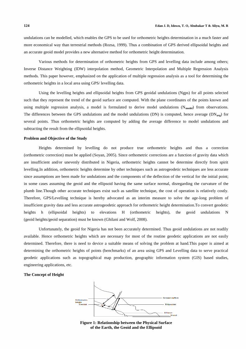
The Concept of Height
Figure 1: Relationship between the Physical Surface
of the Earth, the Geoid and the Ellipsoid
Determination of Orthometric Heights from GPS and Levelling Data 125
The fundamental relationship between ellipsoidal height (h) obtained from GPS measurements and orthometric
heights (H) with respect to a vertical geodetic datum established from spirit levelling data with gravimetric corrections
referred to the geoid is given by Heiskanen and Moritz (1969) and Moka and Agajelu (2006) as:
N = h - H
Thus H = h - N (1)
Where N =geoid undulation/ geoid height
h = ellipsoidal height measured along the ellipsoidal normal
H = orthometric height measured along the curved plumb line.
The GPS observed geoidal undulations can be determined as
Ngps = h – H (2)
Where H = elevations determined by levelling.
The value of Ngps obtained in this manner is to be compared with the values of N from a model and the differences
computed as (Ghilani and Wolf, 2008):
DN = Ngps - Nmodel (3)
To determined the model undulations (Nmodel), we use a base function f(e,n), to functionally represent the geoid
undulations (N) as a function of the coordinates of the points observed (Nwilo et al, 2009) as:
N = h – H = ao + f(e,n) (4)
If the geoid is approximated to a flat surface, which is correct over small areas, then we can write an expression
for N at any point in terms of some base functions which depend on the coordinates of that point. Hence we have:
hi –Hi = Ni = ao + fi(e,n) (5)
The function fi(e,n) can be expressed in terms of linear combination of some base function as (Opaluwa,2008):
fi(e,n) = eix1+ nix2 (6)
Therefore, at any point where ellipsoidal heights from GPS and heights from levelling are known, we can solve
for geiod undulation N, using a least square regression model of the form (Featherstone et al, 1998):
Ni = hi – H = ao + eix1 + nix2 (7)
Where ao = error term,
x1, x2 are tilts of the geoid plane with respect to the WGS84 ellipsoid,
ei and ni are the eastings and northings in the same plane coordinate system.
Using multiple regression analysis, the three parameters (a0, x1 and x2) is determined as follows:
ao = (hi –Hi)mean - x1ê - x2ñ (8)
x1=[∑(℮i-ê)[(h-Ĥ)i-(hi-Ĥi)mean]∑(ni-ñ)2]-[∑(ni-ñ)[(h-Ĥ)i
-(hi-Ĥi)mean]][∑(ei-ê)(ni-ñ)]

126 Edan J. D, Idowu, T. O, Abubakar T & Aliyu, M. R
(∑(ei-ê)2∑(ni-ñ)2)-[∑(ei-ê)(ni-ñ)]2 (9a)
X2=[∑(ni-ñ)[(h-Ĥ)i-(hi-Ĥi)mean]∑(ei-ê)2]-[∑(ei-ê)[(h-Ĥ)i
-(hi-Ĥi)mean]][∑(ei-ê)(ni-ñ)]
(∑(ei-ê)2∑(ni-ñ)2)-[∑(ei-ê)(ni-ñ)]2 (9b)
Equation 7 is formed at the points and solved using multiple regression analysis. The solution yields the value of
the model parameters; ao, x1 and x2, and subsequently the adjusted undulations for the benchmarks. Therefore, the model
undulations are substituted in equation 3 to compute the differences in undulations (DN), hence its average for several
benchmarks in the area. Using an average DN for the survey area, the orthometric heights are computed as
(Ghilani and Wolf, 2008):
H = h – ( Nmodel + DNavg ) (10)
The Study Area
The area of study is High Level ward in Makurdi local government area, Benue State, north-central Nigeria.
The study area has an approximate area of 8.164861742 square kilometres with approximate perimeter of 11.460514
kilometres.
Makurdi, the capital of Benue state is delimited by 16km radius with the centre of the town taken at a control near
the post office. It lies between latitudes 7˚ 28 and 8˚00’ North, and longitude 8˚28’and 8˚35’ East of Greenwich meridian.
It is bounded by Guma local government in the north-east, Tarkaa local government in the east, Gwer local government in
the south, Gwer-West local government in the west and Doma local government area of Nassarawa State in the north-west.
Source: Ministry of Lands & Survey Makurdi
Figure 2: Map of Makurdi Local Government Showing the Distribution of Points in the Study Area
Methodology
The methodology adapted in this study involves data acquisition, data processing, as well as numerical
investigations.
Data Acquisition
Field surveys were conducted to obtain data used in this study. These include heights obtained from spirit
levelling, ellipsoidal heights obtained from GPS as well as positional data using Promark3 GPS receivers. Benchmarks
Determination of Orthometric Heights from GPS and Levelling Data 127
well-dispersed in the area were observed using both GPS and levelling instrument. The GPS was used in static relative
mode for twenty minutes per station with epoch rate of fifteen seconds. Nevertheless, data for existing GPS controls and
levelling benchmarks were obtained from the office of the Surveyor General of the Federation, Makurdi zonal office.
Data Processing
Most of the data utilized in this study were digitally processed using computer hardware and software. Least
squares adjustment of the levelling network was done using WOLFPACK software while positional data from GPS were
done using SURVCARD software.
Equations 2, 3, 7, 8, 9 and 10 were programmed using spreadsheet and solved. Thus, the model parameters
(ao, x1 and x2), GPS observed geoid undulations (Ngps), model undulations (Nmodel), difference in undulations
(DN = Ngps – Nmodel) and its mean (DNavg), orthometric heights (H) were derived. ArcGIS9.2 software was used for
generating the grid map of the area utilizing corrected orthometric heights obtained from equation 10.
Numerical Investigation
The total variation in the dependent variable Ni in equation 2.16 in which Ni is regressed on ‘e’ and ‘n’ in a
3- variable model was tested using the coefficient of multiple determination R2.This coefficient was calculated using the
formula given by Erol and Celik (2003):
R2=(x1 [(h-Ĥ)i-(hi-Ĥi)mean ](℮i-ê)+ x2∑[(h-Ĥ)i -(hi-Ĥi)mean](ni-ñ))
(∑[(h-Ĥ)i-(hi-Ĥi)mean]2 )
-1 (11)
The computed coefficient of multiple determinations was 0.992049442. Generally, the higher the value of R2 the
greater the percentage of variation in Ni explained by the regression model which means also that the better the goodness
of fit of the regression model to the sample observation. Since this value is greater than zero and less than one (0<R2<1),
and also closer to one, it shows that the model is a good fit to the sample observation (Fotopoulos, et al 1999).
Presentation of Results
Since observations were carried out on 85 different stations, the results presented in tabular form became large.
Hence, a sample of each table is hereby presented. The results from observations and computations based on equation 2 are
shown in the Table 1; while results computed from Equations 8 and 9 are in Tables 2 and 3 respectively.
Table 1: Sample Results From Observations and Equation 2
Station No. e (m) n (m) h (m) H (m) Ngps[h-H] (m)
BSS12 450044.111 855487.444 123.99528 105.612 18.38328
H01 449844.023 854987.401 125.44997 106.433 19.01697
H02 449744.172 854687.125 126.67209 107.170 19.50209
H03 449619.166 854462.244 127.52025 107.603 19.91725
H04 449524.521 854137.587 128.52991 108.116 20.41391
H05 449694.482 853737.591 128.93002 108.316 20.61402
- - - - - -
- - - - - -
- - - - - -
H79 448404.268 852850.098 131.11661 109.877 22.23961
H80 447994.118 852897.453 132.64732 110.046 22.60132
H81 447644.562 852946.198 133.46933 110.569 22.90033
∑=38121932.03
ē=448493.318
∑=72574937.540
=853822.7646
∑=1813.2296
=21.33211

128 Edan J. D, Idowu, T. O, Abubakar T & Aliyu, M. R
Table 2: Sample Data for the Computation of Parameters in Equation 8
Stn/No. Ngps – Ñ gps (m) e – ē (m) n – (m) (Ngps– Ñ gps)2 (m
2) (e–ē)
2 (m
2) (n- )
2 (m
2)
BSS12 -2.9488329 1550.790 1664.649 8.69561571 2404958.929 2771057.625
H01 -2.3151429 1350.700 1164.606 5.35988683 1824403.997 1356308.067
H02 -1.8300229 1250.850 864.3304 3.34898396 1564635.729 747067.040
H03 -1.4148629 1125.840 639.4494 2.00183714 1267533.719 408895.535
H04 -0.9182029 1031.200 314.7924 0.84309663 1063379.627 99094.2551
H05 -0.7180929 1201.160 -85.2036 0.51565747 1442794.955 7259.653453
- - - - - - -
- - - - - - -
- - - - - - -
H79 0.90749706 -89.0500 --972.69 0.82355091 7929.902500 946138.6757
H80 1.26920706 -499.200 -925.341 1.61088656 249200.6400 856257.076
H81 1.56821706 -848.756 -876.596 2.45930475 720386.7475 768421.599
∑=92.9637785 ∑=68307748.03 ∑=62416747.33
Table 3: Sample Data for the Computation of Parameters in Equation 9
Stn/No. (e–ē) (n- ) (m) (e–ē) (Ngps– Ñgps) (m) (n- ) (Ngps– Ñ gps) (m)
BSS12 2581526.637 -4573.029482 -4908.772984
H01 1573039.688 -3127.075145 -2696.230285
H02 1081151.138 -2289.091515 -1581.744460
H03 719922.8281 -1592.020611 -904.7332581
H04 324614.8673 -946.8536263 -289.0433072
H05 -102343.497 -862.5473882 61.18410362
- - - -
- - - -
- - - -
H79 86618.63223 -80.81261319 -1174.450092
H80 461930.5267 -633.5881644 -1374.693743
H81 744016.6238 -1331.033639 -1574.851242
∑=4730893.259 ∑=53924.61927
Table 4: Sample Data for the Computation of Parameters in Equation 10
Stn/No. Nmodel (m) DN=Ngps - Nmodel (m) Nmodel + DNavg (m) H = h – ( Nmodel + DNavg ) (m)
BSS12 18.52315259 -0.13987259 18.52378381 105.4714962
H01 19.14067906 -0.12370906 19.14131028 106.3086597
H02 19.49421944 0.00787056 19.49485066 107.1772393
H03 19.80175206 0.115497937 19.80238328 107.7178667
H04 20.17266356 0.241246438 20.17329478 108.3566152
H05 20.38567069 0.228349308 20.38630191 108.5437181
- - - - -
- - - - -
- - - - -
H79 22.27778832 -0.038178315 22.27841954 109.8381905
H80 22.58463032 0.016689683 22.58526154 110.0620585
H81 22.83864120 0.061688801 22.83927242 110.6300576
∑=0.053653453
DÑ=0.0006312170953
Thus the values of the Model parameters; a0, x1, x2 were solved using multiple regression analysis as shown in
Equations 8 and 9. From Tables 2 and 3,
Σ(e-ē)[(h-Ĥ)i-(hi- Ĥi)mean] = 53924.61927 Σ(n-ñ)2 = 62416747.33 Σ(n-ñ)[(h-Ĥ)i-(hi- Ĥi)mean] = 51790.11711
Σ(e-ē)(n-ñ) = 4730893.259 Σ(e-ē)2 = 68307748.03
X1 = -0.0008513726575
Determination of Orthometric Heights from GPS and Levelling Data 129
Similarly, substituting the values in equation 2.18b gives X2 = -0.0008942771399
Substituting X1 and X2 in equation 2.17 gives
a0 = 1166.721268.
Therefore, with the values of a0, x1 and x2, Model 2.16 becomes:
N i= hi-Ĥ = 1166.721268-0.0008513726575ei-0.0008942771399ni+Vi (12)
Where Vi is the error term.
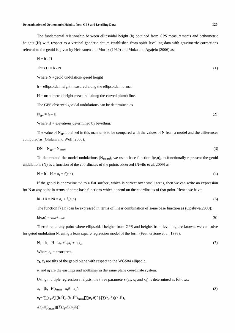
Using Equation 12 the parameters of Equation 3, Model undulations (Nmodel) and Equation 2.19 were computed
and presented in Table 4. The last column of table 4 gives the orthometric heights of the points. The gridded contour map
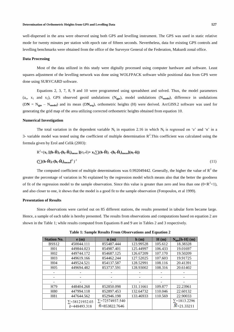
and digital elevation model of the elevations obtained from observations (eqn. 2) were presented in figures 3 and 4, while
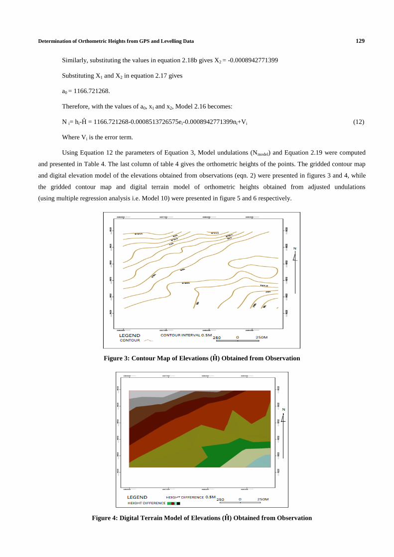
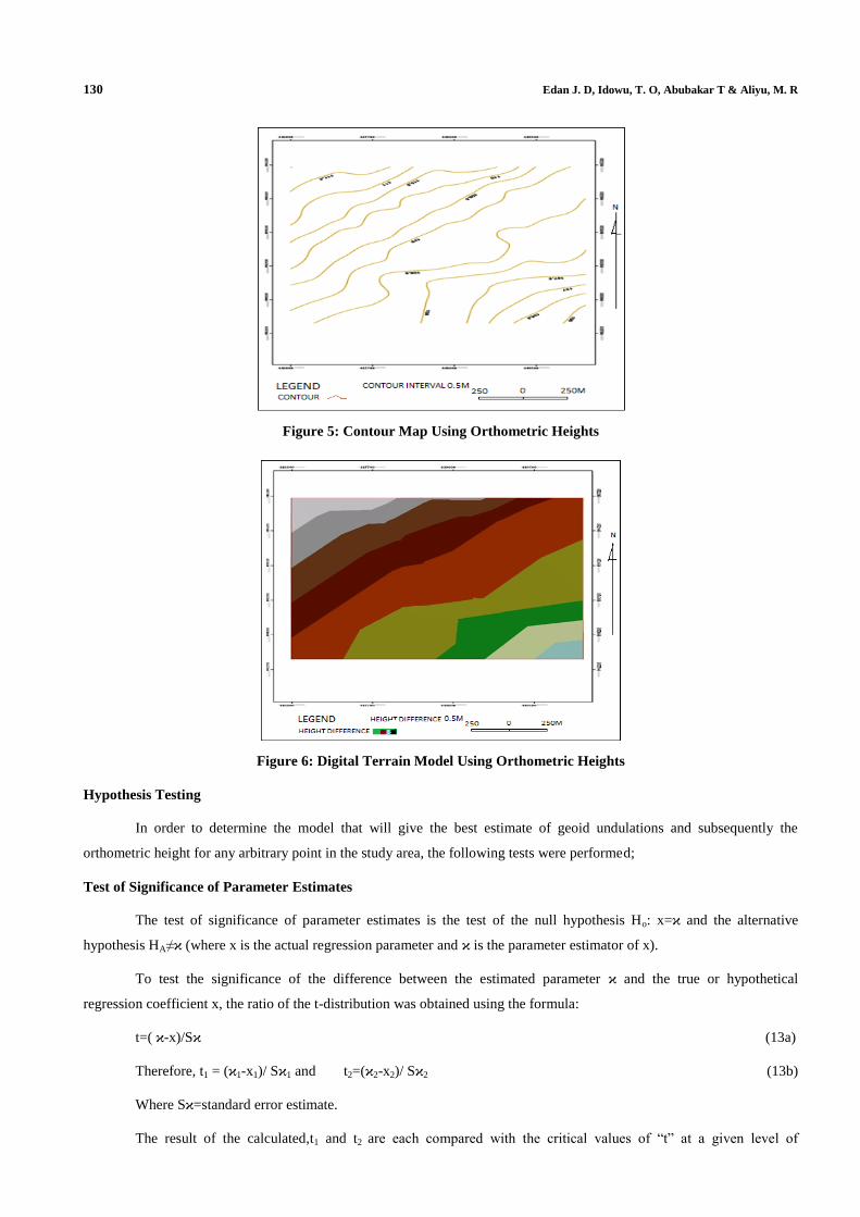
the gridded contour map and digital terrain model of orthometric heights obtained from adjusted undulations
(using multiple regression analysis i.e. Model 10) were presented in figure 5 and 6 respectively.
Figure 3: Contour Map of Elevations (Ĥ) Obtained from Observation
Figure 4: Digital Terrain Model of Elevations (Ĥ) Obtained from Observation
130 Edan J. D, Idowu, T. O, Abubakar T & Aliyu, M. R
Figure 5: Contour Map Using Orthometric Heights
Figure 6: Digital Terrain Model Using Orthometric Heights
Hypothesis Testing
In order to determine the model that will give the best estimate of geoid undulations and subsequently the
orthometric height for any arbitrary point in the study area, the following tests were performed;
Test of Significance of Parameter Estimates
The test of significance of parameter estimates is the test of the null hypothesis Ho: x=ϰ and the alternative
hypothesis HA≠ϰ (where x is the actual regression parameter and ϰ is the parameter estimator of x).
To test the significance of the difference between the estimated parameter ϰ and the true or hypothetical
regression coefficient x, the ratio of the t-distribution was obtained using the formula:
t=( ϰ-x)/Sϰ (13a)
Therefore, t1 = (ϰ1-x1)/ Sϰ1 and t2=(ϰ2-x2)/ Sϰ2 (13b)
Where Sϰ=standard error estimate.
The result of the calculated,t1 and t2 are each compared with the critical values of “t” at a given level of
Determination of Orthometric Heights from GPS and Levelling Data 131
significance (usually 0.05) and degree of freedom N-P. When the value of either t1or t2 exceed the value of critical “t”
obtained from table then ϰ1or ϰ2 is statistically significant and the null hypothesis is rejected. But if t1or t2 or both are less
than or equal to the value of critical “t”, the parameter estimates are not statistically significant.
In this case, the actual regression parameters x1 and x2 are unknown, but it is assumed that whatever value of x
provided, it is less than ϰ and the value of Sϰ is relatively small, “t” calculated must be greater than “t” tabulated. Based on
this assumption, only the standard error of estimates Sϰ1 and Sϰ2 were computed since x1 and x2 are not known.
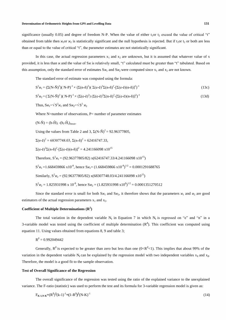
The standard error of estimate was computed using the formula:
S2ϰ1 = (Σ(N-Ñ)
2)( N-P)
-1 × (Σ(n-ñ)
2)( Σ(e-ē)
2Σ(n-ñ)
2-[Σ(e-ē)(n-ñ)]
2)
-1 (13c)
S2ϰ2 = ( Σ(N-Ñ)
2 )( N-P)
-1 × (Σ(e-ē)
2) (Σ(e-ē)
2Σ(n-ñ)
2-[Σ(e-ē)(n-ñ)]
2)
-1 (13d)
Thus, Sϰ1=√ S2ϰ1 and Sϰ2=√ S
2 ϰ2
Where N=number of observations, P= number of parameter estimates
(N-Ñ) = (h-Ĥ)i -(hi-Ĥi)mean.
Using the values from Table 2 and 3, Σ(N-Ñ)2 = 92.96377805,
Σ(e-ē)2 = 68307748.03, Σ(n-ñ)
2 = 62416747.33,
Σ(e-ē)2Σ(n-ñ)
2-[Σ(e-ē)(n-ñ)]
2 = 4.241166098 x10
15
Therefore, S2ϰ1 = (92.96377805/82) x(62416747.33/4.241166098 x10
15)
S2ϰ1 =1.668459866 x10
-8, hence Sϰ1= (1.668459866 x10
-8)
1/2 = 0.0001291688765
Similarly, S2ϰ2 = (92.96377805/82) x(68307748.03/4.241166098 x10
15)
S2ϰ2 = 1.825931998 x 10
-8, hence Sϰ2 = (1.825931998 x10
8)1/2
= 0.0001351270512
Since the standard error is small for both Sϰ1 and Sϰ2, it therefore shows that the parameters ϰ1 and ϰ2 are good
estimators of the actual regression parameters x1 and x2.
Coefficient of Multiple Determinations (R2)
The total variation in the dependent variable Ni in Equation 7 in which Ni is regressed on “e” and “n” in a
3-variable model was tested using the coefficient of multiple determination (R2). This coefficient was computed using
equation 11. Using values obtained from equations 8, 9 and table 3;
R2 = 0.992049442
Generally, R2
is expected to be greater than zero but less than one (0<R2<1). This implies that about 99% of the
variation in the dependent variable Ni can be explained by the regression model with two independent variables x1 and x2.
Therefore, the model is a good fit to the sample observation.
Test of Overall Significance of the Regression
The overall significance of the regression was tested using the ratio of the explained variance to the unexplained
variance. The F-ratio (statistic) was used to perform the test and its formula for 3-variable regression model is given as:
FK-1,N-K=(R2)
2(k-1)
-1+(1-R
2)
2(N-K)
-1 (14)
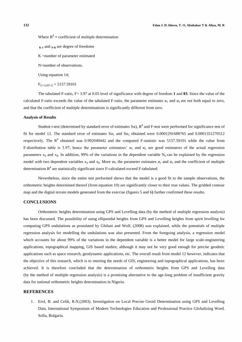
132 Edan J. D, Idowu, T. O, Abubakar T & Aliyu, M. R
Where R2 = coefficient of multiple determination
K-1 and N-K are degree of freedoms
K =number of parameter estimated
N=number of observations.
Using equation 14;
F(2-1),(85-2) = 5157.59101
The tabulated F-ratio, F= 3.97 at 0.05 level of significance with degree of freedom 1 and 83. Since the value of the
calculated F-ratio exceeds the value of the tabulated F-ratio, the parameter estimates ϰ1 and ϰ2 are not both equal to zero,
and that the coefficient of multiple determinations is significantly different from zero.
Analysis of Results
Student t-test (determined by standard error of estimates Sϰ), R2 and F-test were performed for significance test of
fit for model 12. The standard error of estimates Sϰ1 and Sϰ2 obtained were 0.0001291688765 and 0.0001351270512
respectively. The R2 obtained was 0.992049442 and the computed F-statistic was 5157.59101 while the value from
F-distribution table is 3.97; hence the parameter estimators’ ϰ1 and ϰ2 are good estimators of the actual regression
parameters x1 and x2. In addition, 99% of the variations in the dependent variable Ni can be explained by the regression
model with two dependent variables x1 and x2. More so, the parameter estimates ϰ1 and ϰ2 and the coefficient of multiple
determination R2 are statistically significant since F-calculated exceed F-tabulated.
Nevertheless, since the entire test performed shows that the model is a good fit to the sample observations, the
orthometric heights determined thereof (from equation 10) are significantly closer to their true values. The gridded contour
map and the digital terrain models generated from the exercise (figures 5 and 6) further confirmed these results.
CONCLUSIONS
Orthometric heights determination using GPS and Levelling data (by the method of multiple regression analysis)
has been discussed. The possibility of using ellipsoidal heights from GPS and Levelling heights from spirit levelling for
computing GPS undulations as postulated by Ghilani and Wolf, (2008) was explained, while the potentials of multiple
regression analysis for modelling the undulations was also presented. From the foregoing analysis, a regression model
which accounts for about 99% of the variations in the dependent variable is a better model for large scale-engineering
applications, topographical mapping, GIS based studies; although it may not be very good enough for precise geodetic
applications such as space research, geodynamic applications, etc. The overall result from model 12 however, indicates that
the objective of this research, which is to meeting the needs of GIS, engineering and topographical applications, has been
achieved. It is therefore concluded that the determination of orthometric heights from GPS and Levelling data
(by the method of multiple regression analysis) is a promising alternative to the age-long problem of insufficient gravity
data for national orthometric heights determination in Nigeria.
REFERENCES
1. Erol, B. and Celik, R.N.(2003). Investigation on Local Precise Geoid Determination using GPS and Levelling
Data. International Symposium of Modern Technologies Education and Professional Practice Globalizing Word.
Sofia, Bulgaria.

Determination of Orthometric Heights from GPS and Levelling Data 133
2. Featherstone, W.E., Denith, M.C. and Kirby, J.F. (1998). Strategies for Accurate Determination of Orthometric
Heights from GPS. Survey Review. January, PP267-278.
3. Fotopoulos, G., Kotsakis, C. and Sideris, M.G.(1999). Evaluation of Geiod Models and their Use in Combined
GPS/Levelling/Geiod Height Network Adjustment. Technical Reports of the Department of Geoidesy and
Geoinformatics, University Stuttgart.November4.
4. Ghilani, C. D., and Wolf, P.R. (2008). Elementary Surveying: An Introduction to Geomatics.12th
edition, Pearson
Education Ltd, London.
5. Heiskanen, W. A. and Moritz, H. (1969). Physical Geodesy. W.H. Freeman, Austria.
6. Moka, E.C. and Agajelu, S.I. (2006). On the Problems of Computing Orthometric Heights from GPS Data.
Proceedings of the first International Workshop on Geodesy and Geodynamics. November. PP 85-91.
7. Opaluwa, Y.D. (2008). Determination of Optimum Geometrical Interpolation Technique for Modelling Local
Geoid and Evaluation of GPS-Derived Orthometric Height. Unpublished M.Sc. Dissertation, Department of
Surveying and Geoinformatics, University of Lagos, Akoka, Nigeria.
8. Rozsa, S. (1999). Geoid Determination for Engineering Purposes in Hungary. Proceedings of the International
Students’ Conference on Environmental Development and Engineering, pp 125-132, Zakopane.
9. Soyan, M. (2005). A Cost Effective GPS Leveling Method Versus Conventional Leveling Methods For Typical
Surveying Applications, Yildiz Technical University, Istanbul, Turkey.