DETERMINATION OF EVAPORATION AND SEEPAGE LOSSES, UPPER LAKE MARY NEAR FLAGSTAFF, ARIZONA

By J. W. H. Blee

U.S. GEOLOGICAL SURVEY

Water-Resources Investigations Report 87-4250

Prepared in cooperation with the

CITY OF FLAGSTAFF, ARIZONA

Tucson, Arizona May 1988

DEPARTMENT OF THE INTERIOR

DONALD PAUL MODEL, Secretary

U.S. GEOLOGICAL SURVEY

Dallas L. Peck, Director

For additional information Copies of this report can bewrite to: purchased from:

District Chief U.S. Geological SurveyU.S. Geological Survey, WRD Books and Open-File Reports SectionFederal Building, Box FB-44 Federal Center, Bldg. 810300 West Congress Street Box 25425Tucson, Arizona 85701-1393 Denver, Colorado 80225Telephone: (602) 629-6671 Telephone: (303) 236-7476

CONTENTS

Page

Abstract ............................................................ 1

Introduction......................................................... 1

Purpose and scope ............................................. 1

Acknowledgments ............................................... 2

Description of study area ........................................... 2

Instrumentation ..................................................... 4

Measurement of stage and contents ............................. 5

Measurement of mass-transfer variables ......................... 11

Wind measurement ......................................... 11

Psychrometric measurement ................................ 11

Water-surface temperature measurement .................... 15

Evaporation ......................................................... 15

Mass-transfer method ........................................... 16

Mass-transfer coefficient .................................. 16

Evaporation computation ................................... 20

Estimates of mean annual lake evaporation ...................... 21

Method 1 .................................................. 21

Method 2 .................................................. 22

Seepage losses ...................................................... 24

Short-term water budgets ...................................... 26

Relation between stage and seepage ....................... 27

Relation between stage and seepage by selected zones ..... 27

Seepage-duration curve ................................... 34

Distribution of outflow .................................... 35

Sealing of lake bottom ............................................... 35

Conclusions ......................................................... 36

References cited .................................................... 37

Glossary of terms ................................................... 39

V

ILLUSTRATIONS

Page

Figure 1-2. Maps showing:

1. Upper Lake Mary study area ................... 3

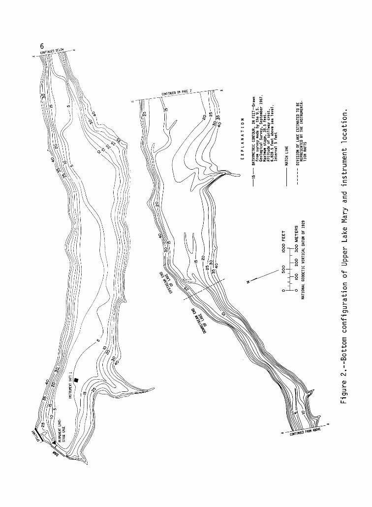
2. Bottom configuration of Upper LakeMary and instrumentation location ............ 6

3. Hydrograph showing contents for UpperLake Mary, 1949-71 ................................ 8

4-8. Photographs showing:

4. Permanent lake-stage gage attached to water- withdrawal tower located at the dam at the downstream end of Upper Lake Mary ......... 9

5. Temporary lake-stage gage located at theupstream end of Upper Lake Mary ............ 10

6. Instrumentation raft 1 located near thedownstream end of Upper Lake Mary ......... 12

7. Digital recorder Smoot servoprogrammer for recording wet-bulb, dry-bulb, and water-surface temperatures ................... 13

8. Automatic motorized psychrometers andradiation shield .............................. 14

9-11. Graphs showing:

9. Estimated average water-surface temperaturesfor Upper Lake Mary ......................... 23

10. Average evaporation rates for evaporation pans at Sierra Ancha and McNary and estimated average evaporation rate for Upper Lake Mary ............................. 25

11. Relation between lake stage and seepage lossdeveloped from short-term water budgets ..... 30

V

ILLUSTRATIONS

Page

Figure 12-14. Graphs showing:

12. Relation between lake stage and surfacearea for Upper Lake Mary .................... 31

13. Relation between lake stage and seepage loss developed from water budgets and lake stage and surface area .................. 32

14. Relations between lake stage and stage duration, stage duration and seepage duration, and seepage duration and seepage ...................................... 33

TABLES

Page

Table 1. Comparison of results between mass-transfer equations3 and 5 ................................................ 19

2. Comparison between evaporation rates measured atrafts 1 and 2 .......................................... 21

3. Summer short-term water-budget computation ............. 28

4. Winter short-term water-budget computation .............. 29

5. Average annual seepage losses, 1950-71 .................. 35

6. Distribution of outflow, 1950-71 .......................... 36

V

CONVERSION FACTORS

For readers who prefer to use the metric (International System) units, the conversion factors for the inch-pound units used in this report are listed below:

Multiply inch-pound unit

inch (in.)

foot (ft)

mile (mi)

acre

acre-foot (acre-ft)

gallon (gal)

ounce (oz)

foot per mile (ft/mi)

acre-foot per day per acre [(acre-ft/d)/acre]

degree Fahrenheit (°F)

25.4

0.3048

1.609

0.4047

0.001233

3.785

0.02957

0.1894

0.0030

'C = 5/9 (°F-32)

To obtain metric unit

millimeter (mm)

meter (m)

kilometer (km)

hectare (ha)

cubic hectometer (hm 3 )

liter (L)

liter (L)

meter per kilometer (m/km)

cubic hectometer per day per hectare [(hm3/d)/ha]

degree Celsius (°C)

Sea level: In this report "sea level" refers to the National Geodetic Vertical Datum of 1929 (NGVD of 1929) A geodetic datum derived from a general adjustment of the first-order level nets of both the United States and Canada, formerly called "Mean Sea Level of 1929."

DETERMINATION OF EVAPORATION AND SEEPAGE LOSSES, UPPER LAKE MARY NEAR FLAGSTAFF, ARIZONA

By

J. W. H. Blee

ABSTRACT

Two mass-transfer equations were developed to compute evapor­ ation as a part of the evaporation- and seepage-loss study for the Upper Lake Mary. Reservoir near Flagstaff, Arizona, which has a capacity of 15,620 acre-feet and a surface area of 876 acres. The mass-transfer equations do not require an independent measure of evaporation to define the mass-transfer coefficient. Data from other evaporation studies were used to define the mass-transfer coefficient as a function of wind shear and atmospheric stability. Long-term seepage losses were determined by use of a seepage-probability curve derived from a stage-seepage relation and defined by several selected short-term water budgets and a lake-stage probability curve. Seepage curves were derived for several different amounts of assumed reservoir sealing. The long-term water savings that would result from each increment of lake-bottom sealing were computed. The study revealed that the evaporation loss was 27 percent or 2,100 acre-feet per year of the total reservoir inflow during 1950-71; seepage loss was 45 percent or 3,500 acre-feet per year.

INTRODUCTION

Upper Lake Mary is about 10 mi southeast of Flagstaff, Arizona, and supplies an average of 75 percent of the water supply for the city. Although the natural water loss from the lake was known to be large, the volume of loss and the amount attributable to seepage and evaporation were not known. During 1964-70, increased withdrawal caused the possibility of a shortage. Artificial sealing of the reservoir to eliminate seepage losses was considered, but information was needed to determine the amount of water that would be saved. A study to evaluate water losses was done in cooperation with the city of Flagstaff.

Purpose and Scope

This report describes the results of a study to determine (1) the evaporation losses, (2) the real and potential seepage losses, and (3) the amount of water savings that would result from total sealing and from different degrees of partial sealing.

1

Modifications of existing techniques were used to determine evaporation and seepage. Evaporation was determined using the mass- transfer equations developed by G. E. Koberg (U.S. Geological Survey, written commun., 1971; written commun., 1972). The techniques define the mass-transfer coefficient as a function of wind shear by using fetch and the ratio of wind speed at 2 and 4 meters above the water surface as an index to wind shear. Seepage was determined by a stage-seepage relation developed from several short-term water budgets. The relation was used in conjunction with 22 years of stage record to define a seepage-probability curve. The curve, in turn, was used to estimate long-term seepage losses.

A set of seepage-probability curves that represented the seepage losses that would occur with various degrees of sealing was defined. The estimated long-term water savings that would result from various degrees of sealing were determined from the probability curves. The ratio for total savings to total area sealed was computed for each interval of partial sealing so that cost-benefit ratios could be determined for the various degrees of sealing.

Acknowledgments

The author wishes to thank Gordon E. Koberg, U.S. Geological Survey, for his assistance and for the use of unpublished work on evaporation mass-transfer equations. James L. Rawlinson and Herman F. Dunnam, Flagstaff City Water Department, provided data from the records of the city of Flagstaff and assisted with the installation of the instruments. Alex M. Sturrock, Jr., and Glenn A. Hearne, U.S. Geological Survey, provided assistance with instrumentation and automatic data processing.

DESCRIPTION OF STUDY AREA

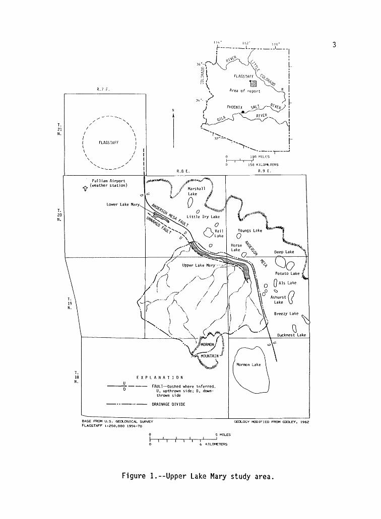
Upper Lake Mary valley is in the high plateau region of north- central Arizona about 10 mi southeast of Flagstaff (fig. 1). The mean annual air temperature in the area of the lake is about 44°F. The mean annual precipitation is about 19 in.; about 11 in. occurs in the form of snowfall. The vegetation consists mainly of Ponderosa pine, scrub oak, and short grasses. Many flat treeless valleys are interspersed in the area. Upper Lake Mary valley is a typical example of these valleys.

The regional water table in the area,is at least several hundred feet below the land surface. Shallow perched water tables occur in a few small valleys. Generally, the lakes in the area are not hydraulically connected with the regional water table. Seepage rates in most lakes are controlled by the porous materials immediately underlying the lakes. Because of unsaturated zones of highly fractured limestone and basalt, most lakes in this region are subject to high seepage losses, particularly

/ II FLAGSTAFF |* /

150 KILOMETERS

R.9 E.

Pul11 am Airport (weather station)

Upper Lake Hary - -^

EXPLANATION

FAULT Dashed where inferred. U, upthrown side; D, down- thrown side

BASE FROM U.S. GEOLOGICAL SURVEY FLAGSTAFF 1:250.000 1954-70

GEOLOGY MODIFIED FROM COOLEY. 1962

I I 1 I6 KILOMETERS

Figure 1.--Upper Lake Mary study area.

artificial lakes that have not existed long enough for thick bottom sediments to have been deposited.

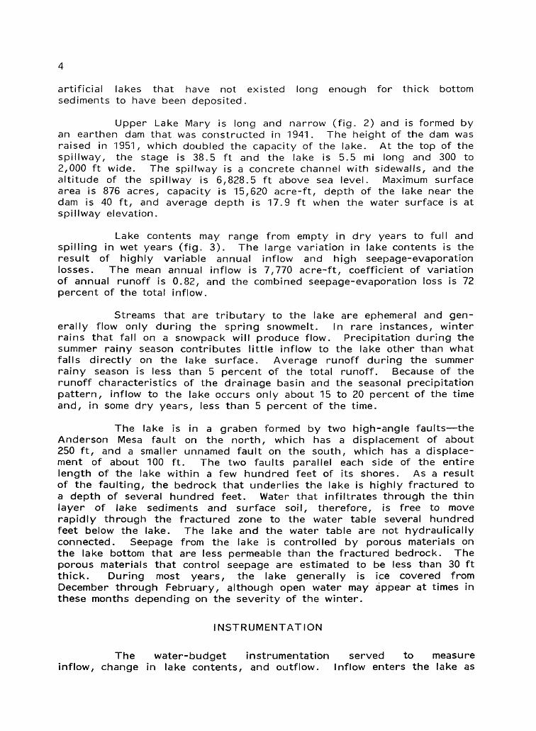
Upper Lake Mary is long and narrow (fig. 2) and is formed by an earthen dam that was constructed in 1941. The height of the dam was raised in 1951, which doubled the capacity of the lake. At the top of the spillway, the stage is 38.5 ft and the lake is 5.5 mi long and 300 to 2,000 ft wide. The spillway is a concrete channel with sidewalls, and the altitude of the spillway is 6,828.5 ft above sea level. Maximum surface area is 876 acres, capacity is 15,620 acre-ft, depth of the lake near the dam is 40 ft, and average depth is 17.9 ft when the water surface is at spillway elevation.

Lake contents may range from empty in dry years to full and spilling in wet years (fig. 3). The large variation in lake contents is the result of highly variable annual inflow and high seepage-evaporation losses. The mean annual inflow is 7,770 acre-ft, coefficient of variation of annual runoff is 0.82, and the combined seepage-evaporation loss is 72 percent of the total inflow.

Streams that are tributary to the lake are ephemeral and gen­ erally flow only during the spring snowmelt. In rare instances, winter rains that fall on a snowpack will produce flow. Precipitation during the summer rainy season contributes little inflow to the lake other than what falls directly on the lake surface. Average runoff during the summer rainy season is less than 5 percent of the total runoff. Because of the runoff characteristics of the drainage basin and the seasonal precipitation pattern, inflow to the lake occurs only about 15 to 20 percent of the time and, in some dry years, less than 5 percent of the time.

The lake is in a graben formed by two high-angle faults the Anderson Mesa fault on the north, which has a displacement of about 250 ft, and a smaller unnamed fault on the south, which has a displace­ ment of about 100 ft. The two faults parallel each side of the entire length of the lake within a few hundred feet of its shores. As a result of the faulting, the bedrock that underlies the lake is highly fractured to a depth of several hundred feet. Water that infiltrates through the thin layer of lake sediments and surface soil, therefore, is free to move rapidly through the fractured zone to the water table several hundred feet below the lake. The lake and the water table are not hydraulically connected. Seepage from the lake is controlled by porous materials on the lake bottom that are less permeable than the fractured bedrock. The porous materials that control seepage are estimated to be less than 30 ft thick. During most years, the lake generally is ice covered from December through February, although open water may appear at times in these months depending on the severity of the winter.

INSTRUMENTATION

The water-budget instrumentation served to measure inflow, change in lake contents, and outflow. Inflow enters the lake as

precipitation on the lake surface and as surface runoff. Precipitation was the only inflow component measured because the water budgets used to define the stage-seepage relation were conducted only during periods of no surface runoff, which eliminated the need for streamflow gages. Changes in lake stage, which were used to determine changes in contents, were recorded at each end of the lake because of the effects of seiches on the water elevation and also to lessen the chance of losing stage record as a result of instrument malfunction. The two forms of measured outflow were withdrawals for city use measured by a recording flowmeter at the city's water-treatment plant and evaporation.

During the 3-year period of collecting continuous stage records, the stage of the lake ranged from 25.2 to 37.2 ft and seiche or oscillation of the water surface occurred almost constantly. Amplitudes were between 0.01 ft and 0.20 ft in a period of about 1 hour. The seiche was mostly wind induced, but the greatest amplitudes were a result of rapid barometric pressure changes associated with local summer thunderstorms moving across the lake. Evaporation was measured by equipment that was installed on rafts anchored near each end of the lake. The reasons for using two rafts were the length of the lake, the differences in topography and tree cover on the prevailing upwind side, and differences in water-surface temperature. The upwind side of the lower half of the lake is a heavily timbered ridge; the upwind side of the upper half of the lake is fairly flat and sparsely timbered. Wind velocities therefore are somewhat higher on the upper half of the lake. Data from a raft at only one end of the lake would not give a true representation of evaporation for the entire lake.

Measurement of Stage and Contents

Two lake-stage gages one at each end of the lake were used to measure changes in lake stage. The gage at the lower end of the lake was a permanent structure attached to the concrete water-withdrawal tower (fig. 4). The stilling well was a 40-foot long, 24-inch-diameter corrugated-metal culvert pipe. The only intake opening to the well was a 0.5-inch-diameter hole about 2 ft from the bottom. The water-stage recorder was housed in a steel shelter. Inside gage heights were measured from a permanent reference mark to the water surface. The gage was operated continuously and was kept free of ice during the winter by an infrared propane heater suspended in the well about 5 ft above the water surface.

The gage at the upper end of the lake was a temporary installation (fig. 5) and was in operation only during May through October. The stilling well was made from a 55-gallon drum with a 0.25-inch-diameter intake hole near the bottom. The drum was held in place by attaching three 2-inch pipes to the drum with U-bolts and then driving a 1.5-inch pipe through the inside of each 2-inch pipe into the bottom of the lake. When the lake level was near the bottom of the gage,

1000

F

EE

T_I

0

100

200

300

ME

TE

RS

NATI

ONA

L G

EODE

TIC

VER

TIC

AL D

ATUM

OF

1929

EXPLANATION

BATHYMETRIC

CONT

OUR,

IN

FE

ET O

rawn

fr

om s

urve

y ma

de by t

he U

.S.

Geol

ogic

al Su

rvey

, September

1967

. Maximum

stage, 3B

.5 fe

et.

Alti

tude

of

spil

lway

cre

st,

6,82

8.5

feet ab

ove

sea

leve

l.

Interval 5

feet

MATC

H LI

NE

DIVISION O

F LA

KE E

STIMATED T

O BE

REPRESENTED

BY T

HE IN

STRU

MENT

A­

TION

RAF

TS

Figu

re 2

.--Bottom

configuration

of U

pper La

ke M

ary

and

inst

rume

nt location.

0 100

200

300 METERS

NATIONAL G

EODE

TIC

VERTICAL D

ATUM

OF

1929 Fi

gure

2.--Continued.

CO

NTE

NTS

, IN

AC

RE-

FEET

00

CQ c. -5

(V C

O o o o -5 c:

-o T3

fD -J n> 10

Figure 4.--Permanent lake-stage gage attached to water-withdrawal tower located at the dam at the downstream end of Upper Lake Mary.

10

Figure 5.--Temporary lake-stage gage located at the upstreamend of Upper Lake Mary.

11

the gage was moved to deeper water. The recorder was housed in a tip-open submersible shelter.

The stage gages were equipped with Stevens A-35 continuous water-stage recorders 1 , which have a gage-height ratio of 10:12 (10 units of change on the chart equal 12 units of change in water level). Both recorders were equipped with 16-inch floats. Measured changes of lake elevation probably were accurate within 0.003 ft.

Measurement of Mass-Transfer Variables

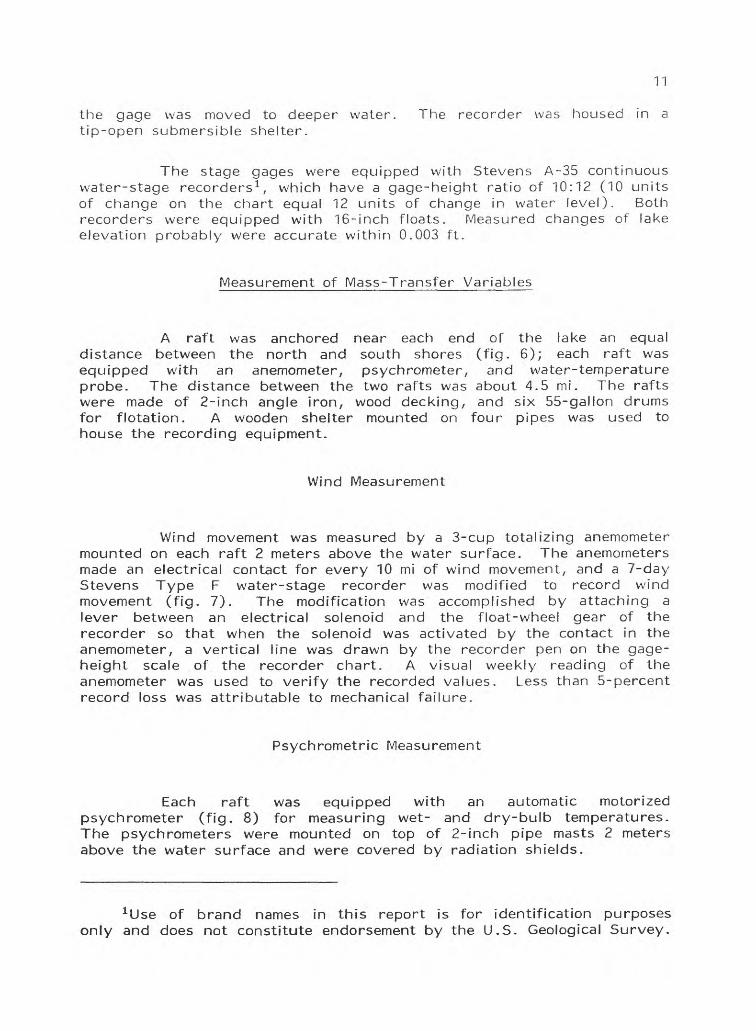
A raft was anchored near each end of the lake an equal distance between the north and south shores (fig. 6); each raft was equipped with an anemometer, psychrometer, and water-temperature probe. The distance between the two rafts was about 4.5 mi. The rafts were made of 2-inch angle iron, wood decking, and six 55-gallon drums for flotation. A wooden shelter mounted on four pipes was used to house the recording equipment.

Wind Measurement

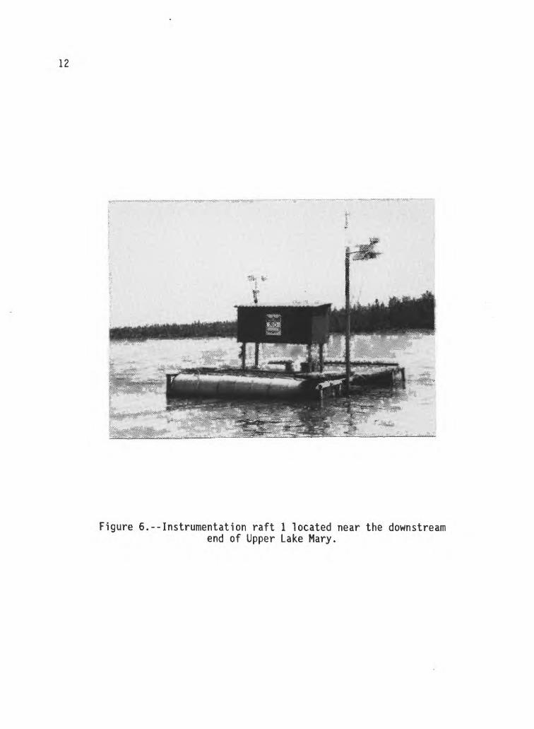
Wind movement was measured by a 3-cup totalizing anemometer mounted on each raft 2 meters above the water surface. The anemometers made an electrical contact for every 10 mi of wind movement, and a 7-day Stevens Type F water-stage recorder was modified to record wind movement (fig. 7). The modification was accomplished by attaching a lever between an electrical solenoid and the float-wheel gear of the recorder so that when the solenoid was activated by the contact in the anemometer, a vertical line was drawn by the recorder pen on the gage- height scale of the recorder chart. A visual weekly reading of the anemometer was used to verify the recorded values. Less than 5-percent record loss was attributable to mechanical failure.

Psychrometric Measurement

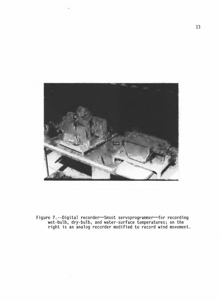
Each raft was equipped with an automatic motorized psychrometer (fig. 8) for measuring wet- and dry-bulb temperatures. The psychrometers were mounted on top of 2-inch pipe masts 2 meters above the water surface and were covered by radiation shields.

1 Use of brand names in this report is for identification purposes only and does not constitute endorsement by the U.S. Geological Survey.

12

Figure 6.--Instrumentation raft 1 located near the downstreamend of Upper Lake Mary.

13

Figure 7.--Digital recorder Smoot servoprogrammer for recording wet-bulb, dry-bulb, and water-surface temperatures; on the right is an analog recorder modified to record wind movement,

14

Figure 8.--Automatic motorized psychrometers and radiation shield. The psychrometer in the center right of photograph is the primary instrument. The psychrometer in the lower left of photograph is an experimental model that was tested for several weeks.

15

The psychrometers consisted of a water reservoir and two temperature probes one wet and one dry mounted inside a 2-inch aluminum tube with a motor-driven fan at the end of the tube. The fan was turned on automatically about 2 minutes before the wet-bulb temperature was recorded to allow enough time for a maximum drop in wet-bulb temperature. Wet- and dry-bulb temperatures were recorded every hour by a 7-channel Smoot servoprogrammer attached to a Fisher-Porter digital recorder. The values recorded on the 16-channel digital-recorder tape were not temperatures but recorder units that had to be converted to temperature when the tapes were processed by computer. During the weekly inspection, a conversion table was used to determine the recorded temperatures. A Bendix motorized psychrometer was used to check and calibrate the recording psychrometers on a weekly basis. The two psychrometer readings generally agreed within 0.3°C. A regression analysis of the data from the two types of psychrometers was made using the Bendix temperatures as the independent variable. A standard least-squares line of best fit showed good correlation between the two instruments; the slope of the least-squares lines was 1.03 and 1.01 for the wet and dry bulbs, respectively.

Water-Surface Temperature Measurement

The water-surface temperature was measured at each raft by a temperature probe at the center of the raft and about 0.5 to 0.75 in. below the water surface. Data were recorded hourly at the same time and in the same manner as the psychrometric temperatures. Water temperatures were checked on a weekly basis with a mercury thermometer and generally agreed within 0.2°C.

EVAPORATION

The mass-transfer method of measuring evaporation was used rather than other available methods, such as pan evaporation or water and energy budgets, because the mass-transfer method offers the best short-term estimate of evaporation loss that can be computed independently of other losses at a moderate cost. A decided advantage of the mass-transfer method was that instruments were readily available that could record the data in a digital form for automatic-data processing.

Although the pan-evaporation method provides an independent measure of evaporation, it is not suitable for computing evaporation for short periods, such as a week or a month, because the coefficient for converting pan-evaporation rates to lake-evaporation rates is unstable and difficult to define except on an annual basis (Ficke, 1972). The water-budget method can be used successfully in some instances, but only if the seepage rates are known or are a negligibly small part of the water-budget residual. In the study of Upper Lake Mary, a water budget

16

was used to define the seepage rates; therefore, the method could not be used as an independent measure of evaporation. The energy-budget method may have been more accurate than the mass-transfer method in the form in which it was used; however, the difference in accuracy, if any, did not justify the additional expense required to install and maintain the instrumentation needed for the energy-budget method.

Mass-Transfer Method

The mass-transfer method of evaporation computation has been used widely. In general, all mass-transfer equations agree that evapora­ tion is proportional to the product of wind speed (£/) times the vapor pressure gradient ( e0 ~ ea )- Marciano and Harbeck (1952) developed a mass-transfer equation that is expressed as:

0 -ea), (D

where

E = evaporation, N = mass-transfer coefficient,U = wind speed at some height above the water surface,

e = saturation vapor pressure that corresponds to thetemperature of the water surface, and

«a = vapor pressure of the air at some height above thewater surface or shore.

One of the difficulties in using equation 1 for measuring evaporation is defining N. In most evaporation studies, N is defined by relating N to some other independent measure of evaporation generally the energy- or water-budget method. At Upper Lake Mary, an independent measure of evaporation was not made. N was determined from empirical equations that were developed by G. E. Koberg (U.S. Geological Survey, written commun., 1971; written commun., 1972).

Two mass-transfer equations were used to compute evaporation. The first equation related N to wind shear by equating wind shear to fetch or distance between the upwind shore and the point of measurement and correcting N for changes in the viscosity of the water. The second equation related N to wind shear by equating wind shear to the ratio of wind speed measured at 2 and 4 meters above the water surface and correcting for atmospheric stability. The second equation was used in the final estimate of evaporation rates.

Mass-Transfer Coefficient

N was determined as a function of wind shear and atmospheric stability (G. E. Koberg, U.S. Geological Survey, written commun., 1971;

17

written commun., 1972). Wind shear is not constant and is a function of water temperature and fetch. Atmospheric stability is a function of the difference in temperature and moisture content between the ambient air and the air that is in contact with the water surface. If the air in contact with the water is colder and drier than the ambient air, a stable condition will exist the air at the water surface is heavier than the ambient air and will not rise. If the air in contact with the water is warmer and has more moisture than the ambient air, the air at the water surface will be lighter, will tend to rise, and create an unstable condition. Because wind shear is a function of more than one variable, a relation that is based on all known variables is difficult to define. Koberg (U.S. Geological Survey, written commun., 1971; written commun., 1972), however, established that a relation exists between water temperature and the ratio of wind speed at 2 and 4 meters above the water surface (Marciano and Harbeck, 1952). The ratio of wind speed is an index to wind shear. The relation indicates that wind shear increases as the temperature of the water surface decreases. The reason for the change in the relation of wind shear to temperature is due to a change in the relation between viscosity and temperature. As the viscosity of water increases, it becomes more difficult for the wind to move the water at the surface. Because water flux is a function of wind shear, a water- temperature correction factor should be applied to equations 1 and 3. The correction factor can be expressed as:

273 \ , (2)273 + T o\

where

TO = the temperature of the water, in degrees Celsius.

Wind shear is also a function of fetch; as fetch increases, wind shear decreases. The reason for the change in the relation between shear and fetch is that the movement of water at the surface tends to approach that of the wind as the water moves downwind. Thus, less energy is expended by the wind in accelerating the water, and in turn, the shear is reduced.

Koberg (U.S. Geological Survey, written commun., 1971) made an analysis to determine if N can be corrected for fetch. The analysis is based on three values of N that were determined by water or energy budgets for Lake Hefner, Oklahoma; Salton Sea, California; and a 1-acre stock pond near Laredo, Texas. The respective values of N are 0.00473, 0.00435, and 0.00510. The respective fetch values are 5,300, 67,000, and 100 ft. The following equation was derived to include the correction for fetch:

0.00510 / x 2 Q\ 0./

550 \ 0.0342 -,650 / o

18

where

E = evaporation, in inches per day;F = fetch, distance from upwind shore to point of

measurement, in feet; TO = the temperature of the water, in degrees Celsius;

U = wind speed at 2 meters above water surface, inmiles per hour;

eQ = saturation vapor pressure that corresponds to thetemperature of the water surface, in millibars; and

e~ - vapor pressure of the air at 2 meters above watersurface, in millibars.

As mentioned previously, N is a function of wind shear, and the 2- and 4-meter wind ratio is an index to the wind shear. Koberg (U.S. Geological Survey, written commun., 1971; written commun., 1972) found in the analysis of N for Lake Hefner, Salton Sea, and the 1-acre stock pond that a relation does exist between the 2- and 4-meter wind ratio and N that can be expressed as:

I/2°- 75(eo-e2 ), (4)

where

U = wind speed at 4 meters above the water surface, in miles per hour.

N also is a function of atmospheric stability. Because equations 3 and 4 do not have a correction for atmospheric stability, their use is limited to conditions of neutral atmospheric stability. High mountain lakes such as Upper Lake Mary, however, are subject to a large degree of atmospheric instability.

Later investigations by Koberg (written commun., 1972) produced an atmospheric stability correction (p~/p0 ) for equation 4:

2 ' 2

where

'0

and

273 + T\ Ip- 0.378e2

S * V 273 + rjU - 0.378e /'

Log = 3.6872 - 2.3283 -^ )- 0.0366t79/ n \ Pf

19

where

p.. =

P n

= density of air at 2 meters above water surface;

density of air at water surface;

air temperature at 2 meters above water surface,in degrees Celsius; andatmospheric pressure, in millibars; andan exponent.

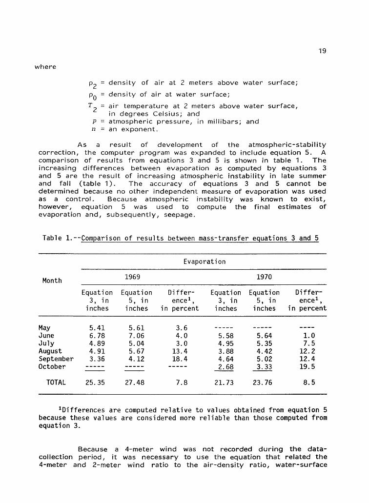
As a result of development of the atmospheric-stability correction, the computer program was expanded to include equation 5. A comparison of results from equations 3 and 5 is shown in table 1. The increasing differences between evaporation as computed by equations 3 and 5 are the result of increasing atmospheric instability in late summer and fall (table 1). The accuracy of equations 3 and 5 cannot be determined because no other independent measure of evaporation was used as a control. Because atmospheric instability was known to exist, however, equation 5 was used to compute the final estimates of evaporation and, subsequently, seepage.

Table 1. Comparison of results between mass-transfer equations 3 and 5

Month

Evaporation

1969 1970

May June July August SeptemberOctober

Equation 3, in inches

5 41 *j » i j_

6.78 4.89 4.91 3.36

Equation 5, in inches

5.61 7.06 5.04 5.67 4.12

Differ­ ence 1 ,

in percent

3 C. b 4.0 3.0

13.4 18.4

Equation 3, in inches

5.58 4.95 3.88 4.642 C.Q. bo

Equation 5, in inches

5.64 5.35 4.42 5.023 33\J +J +J

Differ­ ence 1 ,

in percent

1.0 7.5

12.2 12.4 19 5LJ » %J

TOTAL 25.35 27.48 7.8 21.73 23.76 8.5

Differences are computed relative to values obtained from equation 5 because these values are considered more reliable than those computed from equation 3.

Because a 4-meter wind was not recorded during the data- collection period, it was necessary to use the equation that related the 4-meter and 2-meter wind ratio to the air-density ratio, water-surface

20

temperature, and 2-meter wind speed (G. E. Koberg, U.S. Geological Survey, written commun., 1972). Koberg developed equation 6 from Lake Hefner data and suggested its application to Upper Lake Mary because fetch on both lakes is similar:

P2 (1.80 - 0.0695f/2 )(23.25 - 21.25 )

^ = [1-148 - 0.0008To]( ^ 1 ° , (6)

Evaporation Computation

Wet-bulb, dry-bulb, and water temperatures from the digital tapes were translated to 7-channel magnetic tape. Wind speeds of 6-hour averages were computed manually from the recorder charts, and the data were input to the computer. After the data were translated to 7-channel magnetic tape or put on punch cards and checked, the evaporation computation was made.

The computer program solves equations 3 and 5 for each hourly set of records and prints out the results. Although the computed hourly evaporation rates may be subject to large error, the computation was done in this manner because a sum of the hourly rates will produce a more accurate daily estimate than temperatures that are averaged over a longer period and because the relation between temperature and vapor pressure is curvilinear. At Upper Lake Mary, it is not uncommon to have temperature changes of 15° to 18°C, which may occur in 3 hours or less, during the early morning and evening.

After the daily evaporation rates were determined, the total amount of evaporation for each water-budget period was computed for both rafts, and a weighted average was made for the total lake evaporation. The evaporation rate computed for each raft was weighted by the lake-surface area that the raft represented (fig. 2), therefore,

£-1 A i + E 2 A 2T ~ ~A ~A ' 1 A 1 + A2

where

ET - total lake evaporation,

E~ = evaporation computed from raft 1,

A 1 = lake-surface area represented by raft 1,

#P = evaporation computed from raft 2, and

AQ = lake-surface area represented by raft 2.

21

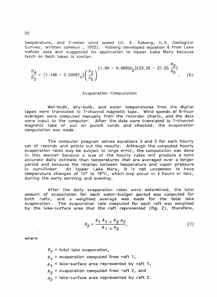
The computed evaporation rates for 1969 and 1970 for each raft and the weighted averages are shown in table 2. The seasonal distribution is somewhat different for 1970 than for 1969 because the lake was thermally stratified in 1969 and nearly isothermal in 1970. The change in lake condition was caused by the installation of an air-bubbling device to artificially induce mixing and keep the lake from thermally stratifying. Mixing the cold water normally found in the hypolimnion with warm water in the eplimnion during May through July reduces the surface temperature and decreases evaporation during those months. Because of the decrease in evaporation rate, there is a net gain in energy from incoming radiation and conduction. More energy is stored in the lake until the surface reaches its normal temperature in late summer (Koberg and Ford, 1965). The net gain in energy is carried over through late summer and early fall and causes a higher-than-normal evaporation rate for the period. The comparison of evaporation rates for rafts 1 and 2 (table 2) illustrates the different rates that can be obtained in a narrow or canyon-type mountain lake because of instrument exposure and location. The comparison points out the need for careful preliminary investigation before placing equipment on such lakes.

Table 2.--Comparison between evaporation rates measured atrafts 1 and 2

Evaporation, in inches

Month

May. ...........June. ..........July. ..........August. ........September. .....October. .......

Raft

4.275.663.984.403 72

1969

1 Raft 2

6.44 7.92 5.69 6.45 4.36

Raft

4.92 4.13 3.16 4.66 3.18

1970

1 Raft 2

6.11 6.16 4.98 5.27 3.44

1969 1970

Weighted mean

5.61 7.06 5.64 5.04 5.35 5.66 4.42 4.11 5.02 3.33

TOTAL. 22.03 30.86 20.50 25.96

Estimates of Mean Annual Lake Evaporation

Method 1

Estimates of mean annual and mean monthly evaporation for Upper Lake Mary were computed by correlating selected meteorological elements that were measured at the Pulliam Airport near Flagstaff and evaporation rates computed from raft-installation data. A least-squares

22

regression analysis was made of computed daily evaporation rates for each raft and the product of:

where

U = daily average wind speed, eo = estimated average daily water-surface temperature

recorded by raft equipment (fig. 9), and e - daily average partial vapor pressure from average

daily dewpoint temperatures measured at PulliamAirport.

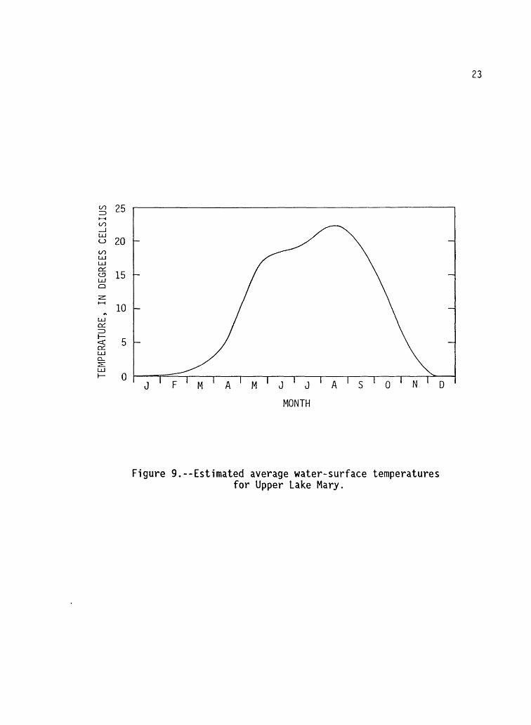
A mass-transfer coefficient for each raft was derived from the regression analysis and was substituted for N in equation 1. Equation 1 was solved for E for each month of the year using the monthly normal temperatures for the terms in equation 8. The water-surface tempera­ tures were determined from (1) recorded temperatures between May and October 1969, (2) miscellaneous temperature measurements, and (3) an estimate of the normal period of ice cover. The sums of the monthly mean evaporation for each raft were then weighted by the estimated area that each raft represented when the lake was at median stage. The total of the weighted sums gave an estimated mean annual lake evaporation of 41.8 in./yr.

The determination of annual evaporation is limited by the estimate of the water-surface temperature from which e0 is computed and the assumption that the relation between lake evaporation and U and ea is the same for the winter ice-covered period as for the May through October open-water period. Because the evaporation rate is small during the winter as compared to the rest of the year, little error is reflected in the annual rate. Kohler and others (1959) indicate that 72 percent of the annual evaporation occurs from May through October.

Method 2

An estimate of mean annual evaporation was made by taking the average May through October evaporation rate for 1969 and 1970 as computed from the raft data and dividing by the average ratio 0.72 of May through October evaporation to the annual evaporation. The estimated mean annual evaporation rate is 41.4 in./yr for Upper Lake Mary.

The estimated monthly evaporation rates were determined by using the average of monthly evaporation for May through October 1969 and for May through October 1970 and subtracting the total for May through October from the mean annual evaporation rate. The remainder was distributed among the months of November through April in the same

23

25GO_UJ<-> 20

15

~ 10*t

UJCti ID h-

Figure 9.--Estimated average water-surface temperaturesfor Upper Lake Mary.

24

proportions as the evaporation rate from the class A pan at Sierra Ancha, which had a 12-month record (fig. 10).

Sierra Ancha is 96 mi south of Upper Lake Mary at 5,100 ft above sea level. The annual evaporation rate, applying a 0.70 pan-to- lake coefficient, is 49.8 in. on the basis of 25 years of record. The average ratio between the May through October evaporation rate and the annual evaporation rate at Sierra Ancha is 0.71.

Another class A evaporation pan is at McNary, Arizona, which is 126 mi southeast of Upper Lake Mary at 7,320 ft above sea level. The pan at McNary is operated only from May through October; however, an annual pan-evaporation rate can be estimated by dividing the evaporation rate from the pan by the ratio of May through October evaporation to the annual evaporation (0.72). An estimated annual pan-evaporation rate of 55 in. multiplied by a pan-to-lake coefficient of 0.70 yields an estimated annual lake evaporation of 39 in. for the station at McNary. The data for McNary compared well with data for Upper Lake Mary.

The seasonal ratios can be applied to annual lake evaporation only for shallow lakes where energy storage can be ignored. At Upper Lake Mary, the data for the May through October evaporation follows the same trend as the data for Sierra Ancha and McNary, which is a good indication that the energy storage is small (fig. 10). If the trend in lake evaporation tends to lag behind pan evaporation in the summer and early fall, energy storage may be large and may cause inaccuracies in the method.

The agreement between the two estimates of annual evaporation is good. An average of the annual rates determined from methods 1 and 2 is used to estimate the average annual lake evaporation. The average of the two methods, rounded to the nearest inch, is 42 in. At a median surface area of 600 acres, the mean annual loss through evaporation is 2,100 acre-ft.

The estimated average monthly lake evaporation (fig. 10) should be used cautiously because it is subject to much more error than the annual rate. Caution is also advised against the use of such estimates for determining monthly evaporation in any given year because the monthly evaporation can vary greatly from year to year depending on changes in conditions, such as thermostratification, depth, inflow, and normal seasonal meteorological changes that do not occur at precisely the same time each year. Method 2, which uses actual measured evaporation for May through October and the ratio of monthly pan evaporation to total evaporation for the remaining months, probably gives the best estimates of average monthly evaporation.

SEEPAGE LOSSES

Seepage losses for Upper Lake Mary were determined from several short-term water budgets that ranged from 3 to 60 days. The

25

12

10

McNaryevaporationpan

UJ:r o

o

O O.<C

Sierra Anchaevaporationpan

Lake Mary evaporation Method 1 Method 2

Jan ' Feb ' Mar ' Apr May I June ' July I Aug ' Sept ' Oct

MONTH

Nov I Dec

Figure 10.--Average evaporation rates for evaporation pans at Sierra Ancha and McNary and estimated average evaporation rate for Upper Lake Mary. Method 1 is from the regression analysis; method 2 is from the ratio of May-October evaporation rate to the total annual evaporation rate.

26

water budgets were computed only for periods of no surface inflow. All the variables in the budgets were measured except seepage, which was computed as a residual. Seepage rates were computed for as many different stages as possible. A relation between stage and seepage was determined from the computed seepage rates and corresponding stages. Using the stage-seepage relation in conjunction with a stage-duration curve, a seepage-duration curve was developed. Because the seepage- duration curve was derived from a long-term record of stage 22 years it can be considered representative of long-term conditions. Therefore, the average annual seepage rate computed from this curve represents the long-term average loss.

Short-Term Water Budgets

Seepage rates were determined from the short-term water budget by using the equation

ip - E - QV , (9)

where

s - seepage, in feet; H« - lake stage at the beginning of the water-budget

period, in feet; H~ = lake stage at the end of the water-budget period,

in feet; ^P = precipitation on the lake surface, in feet;

E - evaporation, in feet; and Qw - withdrawal, in feet.

Changes in storage (#--#-) were determined from recorded

changes in stage. E was measured at the raft installations on Upper Lake Mary. Q was metered by personnel of the city of Flagstaff at the water- treatment plant. I was measured at one rain gage at the upper end of the lake and was used in the water budget only when precipitation represented a small part of the residual. Days having large amounts of precipitation were omitted from the water budgets because an accurate measure of precipitation volume cannot be made by one rain gage owing to the areal variability of the summer rainstorms. Sustained heavy rain may have produced some local runoff around the perimeter of the lake.

After the seepage for a water-budget period was determined, the seepage was divided by the number of days in the period, thereby reducing seepage to a common rate of feet per day. Seepage rates were then adjusted to the viscosity of water at 11 °C, which is the mean water temperature of the lake. During the water-budget periods May through September 1969 and June through October 1970, the lake was at a level that is reached less than 20 percent of the time; therefore, seepage could

27

be determined for stages that seldom occur and when seepage rates are highest (tables 3 and 4).

Because a stage-seepage relation for the full range in stage was needed, seepage rates for stages lower than stages during the study period had to be estimated from records of stage and withdrawal collected by personnel of the city of Flagstaff prior to 1969. Because the stage was read only to the nearest 0.10 ft, water-budget periods were longer than those of 1969-70. The longer periods were used so that the error in determination of the change in lake stage would be a smaller percentage of the water-budget residual.

Generally, November, December, January, and February were the only months for which seepage was computed using only data collected by personnel of the city of Flagstaff. Ice cover was present most of the time, and evaporation rates were low, which reduced the error in the water-budget residual.

Relation Between Stage and Seepage

Seepage is a function of the permeability of the controlling porous material, wetted area, hydraulic gradient, and the viscosity of the water. Because the magnitude of all the components that control seepage may change in relation to stage or time, the relation between seepage and stage is complex.

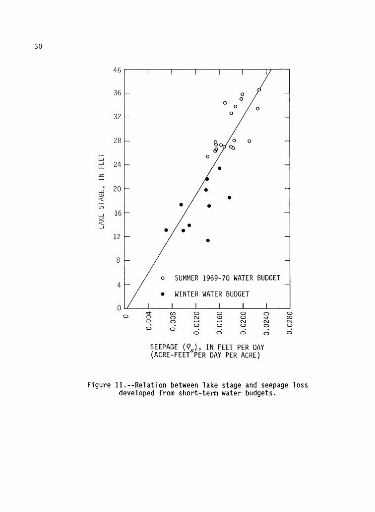
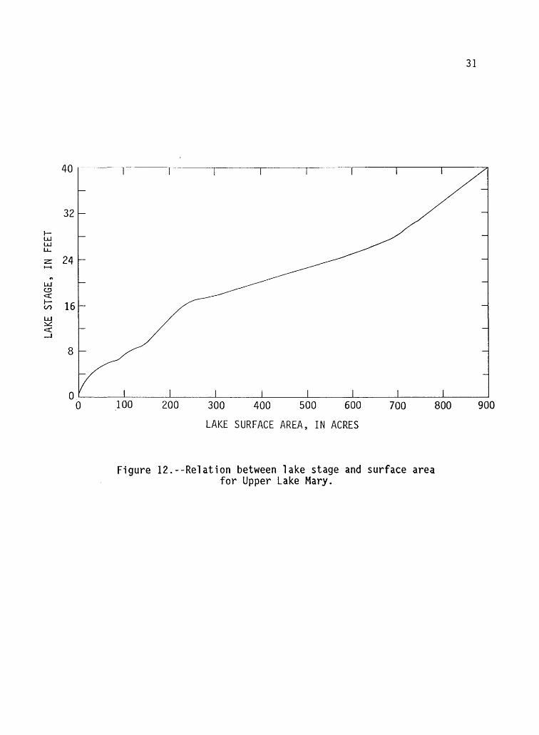
The stage-seepage relation in which seepage is expressed in terms of a volume per unit area rate is shown in figure 11; a total volume rate was computed by applying the unit area rate to the stage-area relation in figure 12. The total volume seepage rate is shown in figure 13. The seepage-loss curve in figure 11 was constructed by plotting the results of the water budgets. The total seepage-loss curve shown in figure 13 was used to compute actual long-term volume losses.

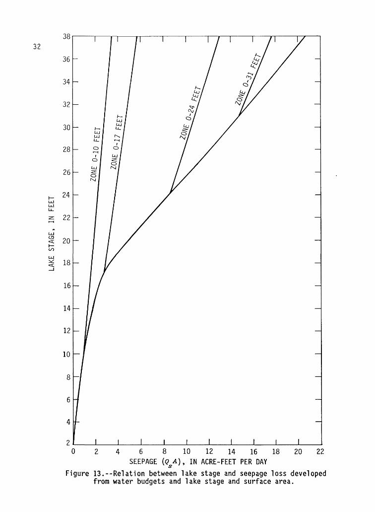
Relation Between Stage and Seepage by Selected Zones

Because part of the objective of the study was to determine the amount of water savings that would result from sealing different amounts of reservoir, estimates of seepage losses through different vertical zones were made. The zones selected for estimating partial seepage losses were for stages 0 to 10 ft, 0 to 17 ft, 0 to 24 ft, and 0 to 31 ft. The set of curves shown in figure 13 and 14 labeled with the appropriate zone is the volume seepage loss that can be attributed to that zone through the entire range in stage. For example, figure 13 shows that in zone 0-24 ft the seepage is about 7.5 acre-ft/d at a lake stage of 24 ft and about 13 acre-ft/d at a lake stage of 38 ft. The stage-seepage curve for any given zone will coincide with the total seepage curve to a stage equal to the top of the zone. For higher stages, seepage through the zone will increase

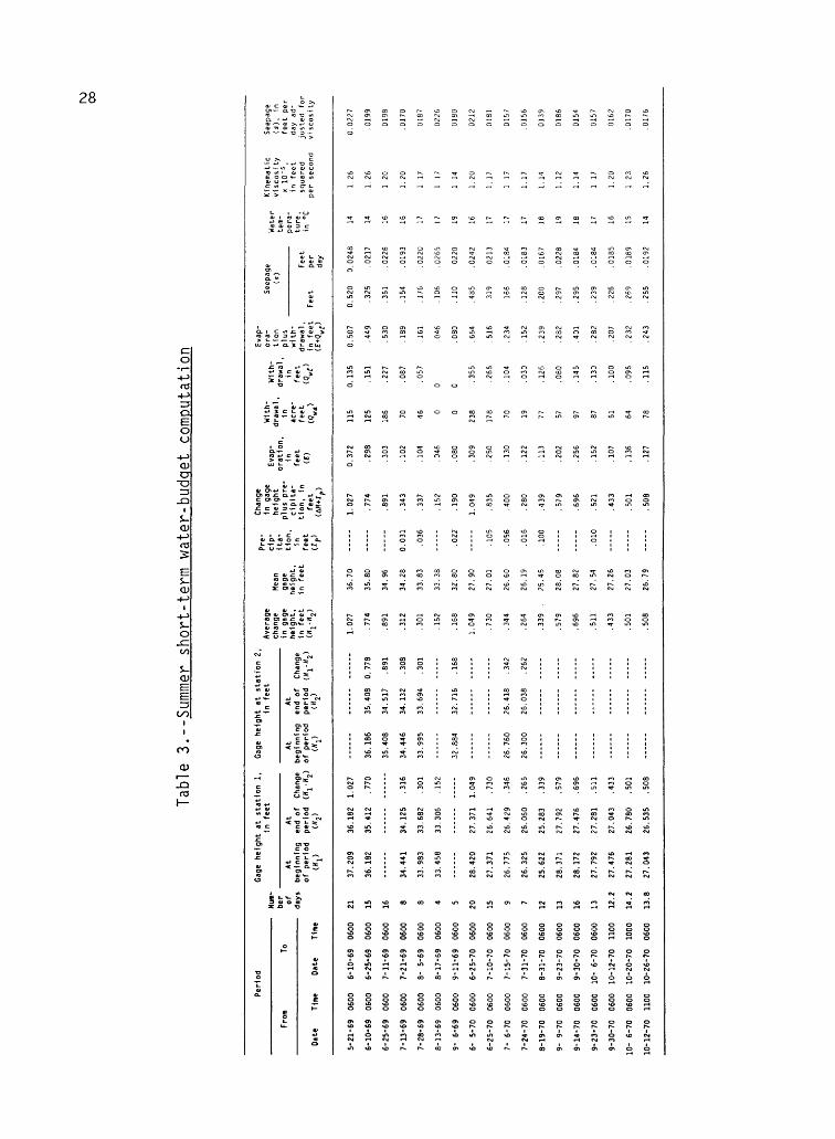
Table

3. --Summer

shor

t-te

rm

Period

From

Date

5-21

-69

6-10

-69

6-25

-69

7-13

-69

7-28-69

8-13-69

9- 6-

69

6- 5-70

6-25-70

7- 6-70

7-24

-70

8-19-70

9- 9-

70

9-14

-70

9-23-70

9-30-70

10-

6-70

Time

0600

0600

0600

0600

0600

0600

0600

0600

0600

0600

0600

0600

0600

0600

0600

0600

0600

To

Date

6-10

-69

6-25-69

7-11-69

7-21-69

8- 5-69

8-17

-69

9-11-69

6-25

-70

7-10-70

7-15

-70

7-31

-70

8-31

-70

9-23-70

9-30

-70

10-

6-70

10-1

2-70

10-2

0-70

Time

0600

0600

0600

0600

0600

0600

0600

0600

0600

0600

0600

0600

0600

0600

0600

1100

1000

Num­

ber

of

da

ys

21

15

16 8 8 4 5 20

15 9 7 12

13

16

13

12.2

14.2

Gage

height at

st

atio

n 1,

Gage

height at station

2,

In feet

In feet

At

begi

nnin

g of pe

riod

37.209

36.1

82

34.4

41

33.9

83

33.458

28.420

27.371

26.7

75

26.3

25

25.6

22

28.3

71

28.1

72

27.792

27.476

27.2

81

At

end

of

period

36.182

35.4

12

34.125

33.682

33.3

06

27.3

71

26.641

26.4

29

26.0

60

25.283

27.792

27.4

76

27.281

27.0

43

26.780

At

At

Chan

ge

begi

nnin

g en

d of

Change

(H^-H2

) of

period

peri

od

(H^-

H^)

.770

36.186

35.408

0.778

.316

34.446

34.132

.308

.301

33.995

33.6

94

.301

.346

26.7

60

26.418

.342

.265

26.3

00

26.038

.262

Average

change

In g

age

heig

ht,

In fe

et

1.027

.774

.891

.312

.301

.152

.168

1.04

9

.730

.344

.264

.339

.

.579

.696

.511

.433

.501

<;nB

Mean

gage

he

ight

, In fe

et

36.7

0

35.8

0

34.96

34.2

8

33.8

3

33.3

8

32.8

0

27.9

0

27.0

1

26.6

0

26. 19

25.4

5

28.0

8

27.8

2

27.54

27.2

6

27.0

3

If. 70

water-budqet co

mput

atio

n

pre.

Ch

ange

ci

p.

In^a

g*

0.03

1 .3

43

.036

.337

-----

.152

.022

.1

90

----

- 1.

049

.105

.835

.056

.400

.016

.280

.100

.439

----

- .5

79

.010

.521

----

- .4

33

----

- .5

01

Evap­

oration,

in

feet

0.37

2

.298

.303

.102

.104

.046

.080

.309

.250

.130

.122

.113

.202

.256

.152

.107

.136

With

­ dr

awal

In

ac

re-

feet

« .>

115

125

186 70

46 0 0

238

178 70

19

77

57

97

87

61

64

Wlth

- '

draw

al ,

in

feet

0.13

5

.151

.227

.087

.057

0 0 .355

.266

.104

.030

.126

.080

.145

.130

.100

.096

Evap­

ora­

tion

plus

with

­ dr

awal

, in

fe

et

0.50

7

.449

.530

.189

.161

.046

.080

.664

.516

.234

.152

.239

.282

.401

.282

.207

.232

Seepage

(*)

Feet

0.52

0

.325

.361

.154

.176

. 106

. 110

.485

319

166

.128

.200

.297

.295

.239

.226

.269

9C-.

Feet

pe

r da

y

0.02

48

.0217

.0226

.0193

.0220

,026

rj

0220

.0242

0213

.018

4

.0183

.0167

.0228

.018

4

.018

4

.0185

.0189

Wate

r te

m­

pera­

ture,

in °C 14

14

16

16

17

17

19

16

17

17

17

18

19

18

17

16

15

Kine

mati

c vi

scos

ity

x ID

'5

, in

fe

et

squared

per

second

1.26

1.26

1 20

1.20

1 17

1 17

1 14

1.20

1. 1

7

1 17

1.17

1. 14

1. 1

2

1.14

1 17

1.20

1 23

r>o 00

Seep

age

(s),

in

fe

et p

er

day

ad­

justed for

visc

osit

y

0.02

27

.0199

0198

.0170

0187

0220

0180

0212

0181

0157

.015

6

0139

0186

0154

0157

0162

.0170

ni7s

Tabl

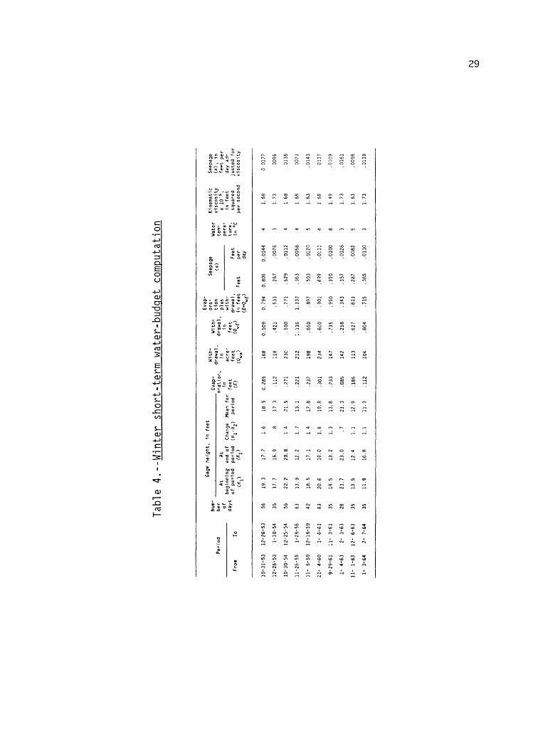
e 4.

--Wi

nter

short-term w

ater

-bud

get

computation

Peri

od

From

10-3

1-53

12-2

6-53

10-3

0-54

11-2

6-55

11-

6-59

11-

4-60

9-29-61

1- 4-63

11-

1-63

1- 3-64

To

12-2

6-53

1-30

-54

12-2

5-54

1-28

-56

12-1

8-59

1- 6-

61

11-

3-61

2- 1-63

12-

6-63

2- 7-64

Num­

ber of days 56 35 56 63 42 63 35 28 35 35

Gage

Atbe

ginn

ing

of pe

riod

19.3

17.7

22.2

13.9

18.5

20.6

14.5

23.7

13.5

11.9

height,

1n fe

et

Aten

d of

Change

period

(tf.

-tf,

)

17.7

1.

6

16.9

.8

20.8

14

12.2

1.7

17.1

1.

4

19.0

1.6

13.2

1.3

23.0

.7

12.4

1.1

10.8

1.1

Evap

-or

atio

n,

Mean

for

peri

od

18.5

17

3

21.5

13.1

17.8

19.8

13.8

23.3

12.9

11.3

7" 0.285

.112

.271

.221

.237

.301

.233

.085

.186

.112

With

­ dr

awal

,

1nac

re-

feet 168

118

230

212

198

234

147

142

113

104

With­

drawal ,

infe

et

«*/>

0.509

.421

.500

1. 116

.660

.600

.735

.258

.627

.604

Evap

­ or

a­

tion

plus

with­

draw

al ,

1n feet

(E-K?^)

0.79

4

.533

.771

1.33

7

.897

.901

.950

.343

.813

.715

Seepage

Feet

0.80

6

.267

.629

.363

.503

.699

.350

.357

.287

.385

Feet

per

day

0.01

44

.0076

.0112

.005

8

.0120

.011

1

.010

0

.012

8

.0082

.011

0

Wate

r Ki

nema

tic

"""

VlSi

o!*t

y£e

ra

in feet

"Po

A sq

uare

d per

seco

nd

4 1.68

3 1.73

4 1

68

4 1

68

5 1.63

4 1

68

8 1.49

3 1.

73

5 1.

63

3 1.73

Seep

age

(s)

, in

feet per

day

ad­

justed for

visc

osi ty

0 0177

0096

.0138

0071

.014

3

0137

.010

9

.016

1

.0098

.0139

ro <£>

30

<: i oo

46

36

32

28

24

20

16

12

o o

o SUMMER 1969-70 WATER BUDGET

WINTER WATER BUDGET

o o

00o o

oC\J

o o

oVO

o o

o oCOo

COo

o00 C\Jo

SEEPAGE (Q), IN FEET PER DAY (ACRE-FEET PER DAY PER ACRE)

Figure 11.--Relation between lake stage and seepage loss developed from short-term water budgets.

31

40

32

UJ UJu_z 24 i i

«\UJ C3

£ 16UJ

.100 200 300 400 500 600

LAKE SURFACE AREA, IN ACRES

700 800 900

Figure 12.--Relation between lake stage and surface areafor Upper Lake Mary.

32

6 8 10 12 14 16 18 SEEPAGE (<? A), IN ACRE-FEET PER DAY

20 22

Figure 13.--Relation between lake stage and seepage loss developed from water budgets and lake stage and surface area.

33

950

98 99 99.5

PERCENTAGE OF TIME THAT A GIVEN STAGE OR SEEPAGE RATE WAS EQUALED OR EXCEEDED

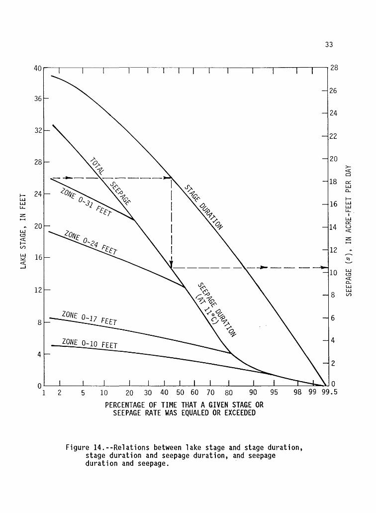
Figure 14.--Relations between lake stage and stage duration, stage duration and seepage duration, and seepage duration and seepage.

34

only as a function of increased head because the area remains constant. For the assumed model, the stage-seepage relation above the stage equal to the top of the zone will be linear because seepage is a linear function of head when all other variables are constant. The surface area and wetted area are considered equal for purposes of analyses because they differ by less than half a percent.

Seepage-Duration Curve

Because seepage rates are a function of stage, actual seepage losses are a function of the characteristics of stage fluctuation, which in turn is a function of reservoir inflow and outflow. Owing to the nonlinear relation between stage and volume rate of seepage (fig. 13), the seepage rate of the average stage of the lake does not necessarily represent the average seepage losses. This is particularly true where the range in stage fluctuation is as great as it is at Upper Lake Mary (fig. 3). Therefore, the actual average total seepage and average seepage losses from the separate zones were determined by seepage- duration curves (fig. 14). The duration curve is a cumulative-frequency curve that shows the percentage of time that a specified component value was equaled or exceeded during a given period. Characteristics of a component throughout the range of values is combined in one curve without regard to sequence of occurrence. A stage-duration curve was derived on the basis of 22 years of stage record, which shows the average percentage of time a particular stage was equaled or exceeded. For example, a lake stage of 26 ft was equaled or exceeded about 45 percent of the time.

A seepage-duration curve was then derived by plotting the seepage rates for the different stages (fig. 13) versus the percentage of time the particular stage was equaled or exceeded. The area under the seepage-duration curves is a measure of the seepage that occurs 100 percent of the time. Dividing the area by 100 gives the average ordinate, which, when multiplied by the appropriate scale factor, will give the average seepage. During 1950-71, the average annual seepage loss was 3,500 acre-ft as determined from an analysis of the seepage-duration curve (table 5).

In a strict sense, the seepage-duration curve applies only to the period for which the data were used to develop the curve. The analysis is based on the assumption that the stage-seepage relation remained constant for the 22-year period and that the annual withdrawal rates also were steady. If, however, the record on which the stage- duration curve is based is large enough to be considered a long-term record, the seepage-duration curve is a seepage-probability curve. The seepage-probability curve may be used to estimate future losses (Searcy, 1959).

35

Table 5.--Average annual seepage losses, 1950-71

Zone

0-10 feet0-17 feet0-24 feet0-31 feet0-38 feet

Average annual loss, inacre-feet

6601,3502,8503,3603,500

Average annual loss peracre, in acre- feet

4.295.365.094.494.04

Average annual seepage,

in percent of total

19498196

100

Zone, in

acres

154252560748866

Percentage of

acres

18296486

100

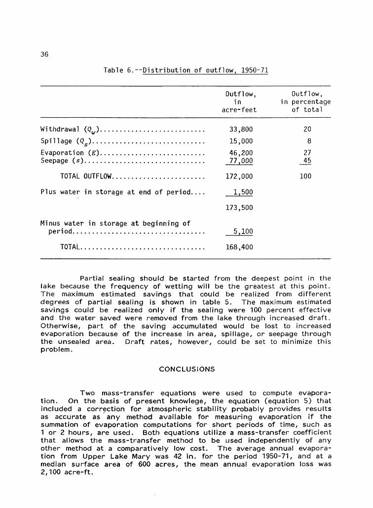
Distribution of Outflow

The different forms of outflow include municipal use, spillage, evaporation, and seepage. Municipal use was determined from city water records, and spillage was determined volumetrically from stage records for Lower Lake Mary. The evaporation and seepage for 1950-71 were determined by multiplying the average annual rates by 22 years. The sum of the computed outflow and the water in storage at the end of the period should equal the total inflow for the 22-year period. As a check on the sum of 168,400 acre-ft, inflow was computed volumetrically from the stage record. The volumetrically computed inflow for the 22-year period equaled 170,890 acre-ft, which is within 1.5 percent of the sum of the computed outflow distribution (table 6).

SEALING OF LAKE BOTTOM

A large percentage of the available water can be saved by total or partial sealing of the lake bottom. The amount of sealing would have to be determined by economic and engineering considerations, which are beyond the scope of this report.

Table 5 shows that the long-term water saving per acre sealed would generally decrease as more area is sealed. The amount of sealing would depend on the results of a cost-benefit study. Sealing the reservoir to a stage of 24 ft, or 64 percent of the area, would result in a savings of 81 percent of the average annual seepage. Sealing to a stage of 31 ft, or 86 percent of the area, would result in a savings of 96 percent of the average annual seepage. The additional 4 percent of the average annual seepage would require the sealing of 100 percent of the reservoir, or an additional 118 acres.

36

Table 6.--Distribution of outflow, 1950-71

Outflow,in

acre-feet

Outflow,in percentage

of total

Withdrawal (Qw )

Spillage (Qs )...

Evaporation (E) Seepage (s)....

TOTAL OUTFLOW.....................

Plus water in storage at end of period.

Minus water in storage at beginning of period...............................

TOTAL.

33,800

15,000

46,20077,000

172,000

1,500

173,500

5,100

168,400

20

8

2745

100

Partial sealing should be started from the deepest point in the lake because the frequency of wetting will be the greatest at this point. The maximum estimated savings that could be realized from different degrees of partial sealing is shown in table 5. The maximum estimated savings could be realized only if the sealing were 100 percent effective and the water saved were removed from the lake through increased draft. Otherwise, part of the saving accumulated would be lost to increased evaporation because of the increase in area, spillage, or seepage through the unsealed area. Draft rates, however, could be set to minimize this problem.

CONCLUSIONS

Two mass-transfer equations were used to compute evapora­ tion. On the basis of present knowlege, the equation (equation 5) that included a correction for atmospheric stability probably provides results as accurate as any method available for measuring evaporation if the summation of evaporation computations for short periods of time, such as 1 or 2 hours, are used. Both equations utilize a mass-transfer coefficient that allows the mass-transfer method to be used independently of any other method at a comparatively low cost. The average annual evapora­ tion from Upper Lake Mary was 42 in. for the period 1950-71, and at a median surface area of 600 acres, the mean annual evaporation loss was 2,100 acre-ft.

37

Computing seepage losses by use of a seepage-duration curve or seepage-probability curve will give an accurate estimate of long-term seepage losses, if all the variables that are used to define the curve are measured accurately. Although this method of determining seepage requires more data reduction and computation time than the conventional water-budget method, it provides more information about the interrelation among components governing seepage and the consequences if one or more of these components is altered.

The average annual seepage loss was computed to be 3,500 acre-ft or 45 percent of the long-term average inflow. Estimates of seepage losses through four selected lake-bottom zones were made to determine the effects of partial sealing. The estimates of seepage through the different zones indicated that the long-term water savings per acre of sealed lake bottom would generally decrease as more area is sealed.

The amount of water that the city of Flagstaff would gain from sealing would depend on the rate at which water was withdrawn from the reservoir. If some of the water saved in storage were allowed to accumulate in the reservoir, the contents and surface area would be larger than normal; therefore, part of the water saved from loss to seepage would be lost to increased evaporation and spillage. An analysis of the economic and engineering feasibility of sealing the reservoir is beyond the scope of this report; however, the hydrologic data needed for such an analysis were collected as part of this study.

REFERENCES CITED

Cooley, M. E., 1962, Physiographic map of the San Francisco Plateau- lower Little Colorado River area: Tucson, University of Arizona, Geochronology Laboratory report.

Ficke, J. F., 1972, Comparison of evaporation computation methods, Pretty Lake, Lagrange County, northeastern Indiana: U.S. Geological Survey Professional Paper 686-A, 49 p.

Koberg, G. E., and Ford, M. E., Jr., 1965, Elimination of thermal stratification in reservoirs and the resulting benefits, hi Contributions to the hydrology of the United States, 1964: U.S. Geological Survey Water-Supply Paper 1809-M, 28 p.

Kohler, M. A., Nordenson, T. J., and Baker, D. R., 1959, Evaporation maps of the United States: U.S. Weather Bureau Technical Paper 37.

38

Marciano, J. J., and Harbeck, G. E., Jr., 1952, Mass-transfer studies, u Water-loss investigations, Lake Hefner studies, technical report: U.S. Geological Survey Professional Paper 269, 158 p.

Searcy, J. K., 1959, Flow-duration curves: U.S. Geological Survey Water-Supply Paper 1542-A, 33 p.

39

GLOSSARY OF TERMS

Terms used in the report are defined below.

Anemometer An instrument that is used for measuring the force or speed of wind.

Atmospheric stability The ratio of the density of the air at a specified point to the air at the water surface.

Epilimnion The upper, warmer, lighter oxygen-rich zone of water that overlies the thermocline.

Fetch The distance that wind blows along open water or land. Also, the distance that waves can travel without obstruction.

Hypolimnion The part of the lake below the thermocline made up of water that is stagnant and of essentially uniform temperature except during periods of overturn.

Isothermal Relating to or marked by equality of temperature.

Mass transfer The concept of the turbulent transfer of water vapor from an evaporating surface to the atmosphere.

Psychrometer A wet and dry bulb-type temperature recorder that measures vapor pressure in the air.

Seiche An oscillation of the surface of a lake or landlocked sea that varies from a few minutes to several hours.

Thermal stratification An air or water mass that is divided into layers by temperature.

Thermocline A layer in a thermally stratified body of water that separates an upper, warmer, lighter oxygen-rich zone (epilimnion) from a lower, colder, heavier oxygen-poor zone (hypolimnion).

Viscosity Property of a fluid that enables it to develop and maintain an amount of shearing stress dependent upon the velocity of flow and then to offer continued resistance to the flow.

Water flux The continuous movement of water.

Wind shear The action of the wind on the water.