DETERMINANTS OF STOCK MARKET VOLATILITY: EVIDENCE FROM MALAYSIA...
108
A01 DETERMINANTS OF STOCK MARKET VOLATILITY: EVIDENCE FROM MALAYSIA BY CALEB CHAN JIA-LE CHEONG TZUN HOE FOO WEN SENG HENG ZHEN XUAN HO YONG FENG A research project submitted in partial fulfillment of the requirement for the degree of BACHELOR OF FINANCE (HONS) UNIVERSITI TUNKU ABDUL RAHMAN FACULTY OF BUSINESS AND FINANCE DEPARTMENT OF FINANCE AUGUST 2015
Transcript of DETERMINANTS OF STOCK MARKET VOLATILITY: EVIDENCE FROM MALAYSIA...

A01
DETERMINANTS OF STOCK MARKET
VOLATILITY: EVIDENCE FROM MALAYSIA
BY
CALEB CHAN JIA-LE
CHEONG TZUN HOE
FOO WEN SENG
HENG ZHEN XUAN
HO YONG FENG
A research project submitted in partial fulfillment of the
requirement for the degree of
BACHELOR OF FINANCE (HONS)
UNIVERSITI TUNKU ABDUL RAHMAN
FACULTY OF BUSINESS AND FINANCE
DEPARTMENT OF FINANCE
AUGUST 2015

Determinants of Stock Market Volatility
ii
Copyright @ 2015
ALL RIGHTS RESERVED. No part of this paper may be reproduced, stored in a
retrieval system, or transmitted in any form or by any means, graphic, electronic,
mechanical, photocopying, recording, scanning, or otherwise, without the prior
consent of the authors.

Determinants of Stock Market Volatility
iii
DECLARATION
We hereby declare that:
(1) This undergraduate research project is the end result of our own work and that
due acknowledgement has been given in the references to ALL sources of
information be they printed, electronic, or personal.
(2) No portion of this research project has been submitted in support of any
application for any other degree or qualification of this or any other university, or
other institutes of learning.
(3) Equal contribution has been made by each group member in completing the
research project.
(4) The word count of this research report is 15,769 words.
Name of Student: Student ID: Signature:
1. Caleb Chan Jia-Le 1301022
2. Cheong Tzun Hoe 1200304
3. Foo Wen Seng 1300664
4. Heng Zhen Xuan 1300109
5. Ho Yong Feng 1106494
Date: 1st September 2015

Determinants of Stock Market Volatility
iv
ACKNOWLEDGMENT
First and foremost, we are grateful to God for the good health and wellbeing that
were necessary to complete this research.
We are grateful to Encik Aminuddin Bin Ahmad, our main supervisor, for the
provision of expertise, and technical support. Without his superior knowledge and
experience, we wouldn’t have achieved this outcome. He is like a mentor and
friend, guiding us through the research. We truly are thankful to be under his
supervision.
We are also grateful to Ms Chia Mei Si, our second examiner, in the Department
of Finance. We are extremely thankful and indebted to her for sharing expertise,
and sincere and valuable guidance and encouragement extended to us.
We would like to take this opportunity to express gratitude to all of the department
faculty members for their help and support. We also thank our parents for the
unceasing encouragement and support.
We also place on record, our sense of gratitude to one and all, who directly or
indirectly, have lent their hand in this exciting research.

Determinants of Stock Market Volatility
v
TABLE OF CONTENTS
Page
Copyright Page……………………….…………………………………….... ii
Declaration ………………………………………………………………….. iii
Acknowledgement…..……………………………………………………….. iv
Table of Contents …………………………………………………………..v-ix
List of Tables ………………………………………………………………….x
List of Figures ………………………………………………………………..xi
List of Abbreviations …………………………………………………...…...xii
List of Appendices…………………………………………………………..xiii
Preface ………………………………………………………………………xiv
Abstract……………………………………………………………………... xv
CHAPTER 1 INTRODUCTION ………………………………………...1
1.1 Research Background…………………………………...1-3
1.2 Problem Statement………………………………………3-5
1.3 Research Objectives……………………………………….5
1.3.1 General Objective………………………………….5
1.3.2 Specific Objective……………………………….5-6
1.4 Research Questions………………………………………..6
1.5 Hypothesis of the study………………………………….6-7
1.6 Significance of Study……………………………………7-8
1.7 Chapter Layout…………………………………………8-10
1.8 Conclusion………………………………………………..10

Determinants of Stock Market Volatility
vi
CHAPTER 2 LITERATURE REVIEW…….….……….……………...11
2.0 Introduction….…………………………………………...11
2.1 Literature Review……….………………………………..11
2.1.1 Stock Index…………………………………...11-13
2.1.2 Interest Rate……......…………………………13-15
2.1.3 Exchange Rate………………………………..15-17
2.1.4 Inflation Rate…………………………………17-19
2.1.5 Gross Domestic Production Growth Rate……19-21
2.2 Review of Relevant Theories…………………………….21
2.2.1 Stock Price……………………………………….21
2.2.1.1 Arbitrage pricing theory…………………21
2.2.2 Interest Rate……………………………………...22
2.2.2.1 Dividend Discount Valuation Model…22-23
2.2.3 Exchange Rate……………………………………23
2.2.3.1 The Classical Economy Theory………23-24
2.2.3.2 Good Market Theory………………….24-25
2.2.4 Inflation Rate……………………………………..25
2.2.4.1 Fisher Effect Hypothesis……………...25-26
2.2.5 Growth Domestic Production Growth Rate……...26
2.2.5.1 The Flight-to-Quality Behavior Theory.....26
2.2.6 Relevant Theoretical Framework……………..26-27
2.3 Proposed Theoretical Framework……………………......27
CHAPTER 3 METHODOLOGY…………………………………….....28
3.0 Introduction………………………………………………28
3.1 Research Design………………………………………….28
3.2 Data Collection Method………………………………….28

Determinants of Stock Market Volatility
vii
3.2.1 Secondary Data…………………………………..29
3.3 Data Processing Procedures……………………………...30
3.4 Economic Regression Model…………………………30-31
3.5 Econometric Method and Data Analysis………………....31
3.5.1 Introduction to Eviews 6…………………………31
3.5.2 P-value………….………………………...………32
3.5.3 T-statistic Hypothesis Test……………………32-34
3.5.4 Multicollinearity…………...............................34-35
3.5.5 Heteroscedasticity…………………………….35-37
3.5.6 Autocorrelation……………………………….37-38
3.6 Conclusion………………………………………………..38
CHAPTER 4 DATA ANALYSIS………………………………………39
4.0 Introduction………………………………………………39
4.1 Diagnostic Checking……………………………………..39
4.1.1 Jarque-Bera Normality Test (JB Test)………..39-40
4.1.2 Ramsey’s Regression Specification Error Test…..40
4.1.3 Heteroscedasticity Test…………………………...41
4.1.4 Autocorrelation…………………………………...42
4.1.5 Multicollinearity Test…………………………….43
4.1.5.1 High 𝑅2 but few Significant t-ratios……..43
4.1.5.2 High pairwise correlation among X’s……44
4.1.5.3 Variance Inflation Factor (VIF)………….44
4.1.5.4 Tolerance Factor (TOL)………………….45
4.2 Hypothesis Testing……………………………………….46
4.2.1 Hypothesis for Model Fit (F-test)...………………46
4.2.2 Hypothesis Testing (t-test)……………………46-47

Determinants of Stock Market Volatility
viii
4.2.2.1 Interest Rate………………………………47
4.2.2.2 Inflation Rate……………………………..48
4.2.2.3 Gross Domestic Production…………..48-49
4.2.2.4 Exchange Rate……………………………49
4.3 Interpretation……………………………………………..49
4.3.1 Parameters Interpretation……………………..49-50
4.3.2 Goodness of Fit…………………………………..50
4.4 Conclusion………………………………………………..51
CHAPTER 5 DISCUSSION, CONCLUSION AND IMPLICATION….52
5.0 Introduction………………………………………………52
5.1 Summary of Results…………………………………..52-53
5.2 Discussion of Major Findings……………………………53
5.2.0 Expected Sign vs. Actual Output………………...53
5.2.1 Interest Rate…………………………………..53-56
5.2.2 Inflation Rate…………………………………56-57
5.2.3 GDP Growth Rate……………………………57-58
5.2.4 Exchange Rate………………………………...58-60
5.3 Implication of this Study…………………………………61
5.3.1 Interest Rate…………………………………..61-62
5.3.2 Inflation Rate…………………………………62-63
5.3.3 GDP Growth Rate……………………………63-65
5.3.4 Exchange Rate………………………………..65-67
5.4 Limitation of this Study………………………………….67
5.4.1 Stock Index Restriction…………………………..67
5.4.2 Debatable Sample Size…………………………...68
5.4.3 Limitation of Linear Regression Method………...68

Determinants of Stock Market Volatility
ix
5.4.4 Findings is Subjected to Malaysia only…………..68
5.5 Recommendation for Future Research…………………...69
5.5.1 Substitution of FTSE stock index………………...69
5.5.2 Conduct Future Research in Different Countries
with Dual Financial System…………………………..69-70
5.6 Conclusion……………………………………………….70
References ………………………………………………………….…….71-83
Appendices …………………………………………………………….....84-93

Determinants of Stock Market Volatility
x
LIST OF TABLES
Page
Table 3.1: Data Sources 29
Table 4.1: JB Normality Test Output 39
Table 4.2: Ramsey’s Regression Specification Error Test Output 40
Table 4.3: Correlation Analysis 44
Table 4.4: Pearson’s Correlation Coefficient Range Table 44
Table 4.5: Variance Inflation Factor (VIF) 45
Table 4.6: Tolerance Factors 45
Table 5.1: Summary Result of OLS Regression 52-53

Determinants of Stock Market Volatility
xi
LIST OF FIGURES
Page
Figure 2.1 Theoretical Framework By Schwert (1989) 27
Figure 2.2 Proposed Theoretical Framework 27
Figure 3.1 Illustration of Data Processing 30
Figure 3.2 Normal Distribution Curve 33
Figure 3.3 Variance of Error Term 35
Figure 3.4 Processes to Detect Heteroscedasticity 36
Figure 3.5 Distribution of Error Term 37
Figure 5.1 Relationship Between Exchange Rate and Stock Market Index 59
Determinants of Stock Market Volatility
xii
LIST OF APPENDICES
Page
Appendix 4.1: Jarque-Bera Normality Test Output 84
Appendix 4.2: Ramsey’s Regression Specification Error Output 85
Appendix 4.3: Heteroscedasticity Test: Breusch-Pagan-Godfrey Test Output 86
Appendix 4.4: Autocorrelation: Breusch-Godfrey Serial Correlation LM Test
Output 87
Appendix 4.5: Auxiliary Model 1 88
Appendix 4.6: Auxiliary Model 2 89
Appendix 4.7: Auxiliary Model 3 90
Appendix 4.8: Auxiliary Model 4 91
Appendix 4.9: OLS Final Output 92
Appendix 5.0: Correlation Output 93

Determinants of Stock Market Volatility
xiii
LIST OF ABBREVIATION
APT Arbitrage Pricing Theory
ARCH Autoregressive Conditional Heteroscedasticity
BLUE Best Linear Unbiased Efficient
CAPM Capital Asset Pricing Model
CLRM Classical Linear Regression Model
CPI Consumer Price Index
EXC Exchange Rate
FDI Foreign Direct Investment
FTSE Financial Times Stock Exchange
GDP Gross Domestic Production
INT Interest Rate
IPO Initial Public Offering
JB Jarque-Bera
KLCI Kuala Lumpur Composite Index
KLSE Kuala Lumpur Stock Exchange
LM Test Breusch Godfrey Langrange Multiplier Test
MUI Market Uncertainty Index
OLS Ordinary Least Square
OPR Overnight Policy Rate
RESET Ramsey’s Regression Specification Error Test
SC Security Commission
UK United Kingdom
US United States
VIF Variance Inflating Factor

Determinants of Stock Market Volatility
xiv
PREFACE
Market participant are concern with the volatility of stock market.
Macroeconomic can determine the stock market fluctuation in the market. By
proving the relationship between the macroeconomic variables and the stock
market, market participant can interpret and understand the volatility of stock
market more accurately and precisely.
Besides that, this research also includes the implication for various market
participants that are actively engaging in investment activities in the Malaysia
stock market.
This research is intended to establish a significant contribution to those parties
who have concerns about Malaysia stock price fluctuations as well as macro
financial environment of Malaysia.

Determinants of Stock Market Volatility
xv
ABSTRACT
This paper studied the four macroeconomic determinants of FTSE Kuala Lumpur
Composite Index volatility from 1980 to 2013 which consists of annual data of 34
sample sizes. The four macroeconomic variables are inflation rate, interest rate,
exchange rate, and gross domestic production (GDP). This study used Ordinary
Least Square (OLS) method to compute the statistical result. Based on the result,
all the variables are significant except for interest rates. According to the
statistical relationships, there are some inconsistencies between the actual and
expected outcome for inflation rate and interest rate.

Determinants of Stock Market Volatility
Page 1 of page 93
CHAPTER 1: RESEARCH OVERVIEW
1.0 Introduction
The main highlight of this chapter is on the backgrounds of this research, problem
statements, objectives, hypothesis, as well as the significance of this study. The
layouts for the following chapters are also included together with the conclusion
for this chapter.
1.1 Research Background
When people talk about stocks, it usually refers to the companies that are listed on
the stock exchange all around the world. In 1300s, the Venetians were the first to
trade securities with governments by using slates with information for sale and
meet clients which act like brokers nowadays. In 1531, Belgium started the first
stock exchange- Sans stock exchange, which brokers and moneylenders would
meet there to make dealing with notes and bonds which is quite odd. In fact in
1500s, there was no real stock. Then in 1600s France, Britain and the Netherlands
chartered voyages to the East Indies, it is very risky as the weather is
unpredictable, navigations is poor and there were pirates back in the days. So to
lessen the risk, ship owners seek investors to put money for the voyage and they
will give part of their revenue to the investors if the voyage was successful. Those
are the starting point of investment in stock market and it evolved into electronic
stock exchange that we use to make investments in domestic or foreign stock
market today.
Based on Capital Markets and Services Act 2007, Kuala Lumpur Stock Exchange
(KLSE) is a financial institution which categorized under stock exchange industry
in Malaysia. Bursa Malaysia provides various services such as trading, depository

Determinants of Stock Market Volatility
Page 2 of page 93
services, clearing and settlement. In fact, it plays an important part in Malaysia’s
open market for large organization and government to raise capital (Erzen, 1995).
KLSE has established sophisticated system to facilitate the computerization of
services and process in order to improve the market efficiency and infrastructure
in the mid-1990s. On the other hand, the initial public offerings (IPO) and the
equity investment have also been reviewed. As a result, some of big privatized
companies such as TenagaNasionalBerhad and Telekom Malaysia Berhad were
listed on KLSE and led to fast growing in the market. In addition, KLSE and
Securities Commission (SC) have work together to improve the transparency of
the market, disclosure, accounting and corporate governance. Unfortunately, the
degree of conformation is still under the international standard. So, most of the
investors are focused on short-term placements instead of long-term. In order to
promote long-term investment, the issuers tend to increase the dividend payments
(Shimomoto, 1999).
According Asian Institute of Chartered Bankers, the equity market is a place that
provides a trading platform for those corporations that wish to raise fund through
equity by issuing new stocks on Bursa Malaysia. Equity market can spread into
two main sectors. The primary market operates with the objective to raise the new
funds for enterprises whereas secondary market is to provideinvestment liquidity
for investors to achieve investment goals.
KLCI is calculated based on 86 major Malaysian stocksusingpaasche formula and
with 1977 as the base level. In 1995, KLSE has 492 listed companies (Yao &Poh,
1997). The Malaysian stock market was set in year 1986 with 70 constituents and
it increased to 100 in 1995. While in 2009, the indices split into two new indices
which are FTSE BM KLCI 30 (KLCI) and FTSE BM MID 70 (KLCI 70)
(Azevedoet al., 2014). Malaysia’s stock market was the fifth biggest share market
in terms of market capitalization prior to the Asian financial crisis (Poobalan,
2001).
Walid, Chaker, Masood and Fry (2011) has stated that stock market crash (1987),
Mexican currency crisis (1994), Asian currency crisis (1997) and the subprime
loan crises (2007 -2008) had been experienced by emerging countries. These

Determinants of Stock Market Volatility
Page 3 of page 93
crises have brought big impact to the world as it reduced the confidence of
investors which reduced the volume of investments in the stock market. It then
influenced corporations as they cannot get the funds that they needed for
development of businesses and eventually brought negative impact to the
countries’ economy.
In the earlier 1990s, Malaysia uses monetary policy strategy to control inflation in
Malaysia by adjusting its interest rate. Later, Bank Negara Malaysia (BNM) had
implied the Overnight Policy Rate (OPR) as a new framework in April 2004 in
order to raise the effectiveness of its monetary policy. It provided a signal to the
market on the posture of monetary policy and acts as a target rate for Bank Negara
Malaysia’s daily liquidity operations (Goh and McNown, 2015). “Malaysia
current monetary policy is still providing an essential support to economic growth
adequately”, said Tan Sri Dr ZetiAkhtar Aziz, Bank Negara Governor (The Star,
2013).
Previous studies have been very useful and provided much important information
regarding the field of stock market research. Several studies also studied the
relationship between macroeconomic factors and stock market return.
Nevertheless, results generated by previous authors are not conclusive. Abrugi
(2008) stated that large gap still exist in the identification of relationship between
macroeconomic factors and return, especially emerging market. Therefore, this
study intends to serve as a bridge to identify any linkage between the selected
macroeconomic variables and stock equity market return in Malaysia.
1.2 Problem Statement
Policy makers and many market practitioners have been studying the origins of
the equity market fluctuation for long time. The main objective of policy maker is
to identify the determinants of equity market and the effects and consequences of
manipulating the macroeconomics variable to the country economic while the
market practitioners focus on the use of the financial instruments to speculate or

Determinants of Stock Market Volatility
Page 4 of page 93
hedge the equity market. Both of the parties have the same objective which is
speculating profit and manage the risk exposure in the equity market by using the
fundamental analysis on the future outlook of the economic factors. Abugri (2006)
stated that there are many theoretical justifications to justify the relationship
between macroeconomic factors and stock return. Besides, market participants
also paid attention to the news of economic outlook and changes of the country
policy. Therefore, large corporation may be put at risk if they are unable to detect
or predict any movement in the stock market due to changes or manipulation of
macroeconomic factors. In fact, certain risk may also be reduced to a minimal
level if the important factors can be taken into consideration and monitor
frequently.
Many previous studies have contributed to the literature of this field (Maskay and
Chapman, 2007; Cook and Halm, 1988; Tsai, 2012; Feldstien, 1978).
Unfortunately, the results of the empirical analysis are still ambiguous due to
many factors such as different economy cycle stages, exchange rate policy,
currency control policies and etc.
Another inconsistency of findings can also be found regarding the relationship
between interest rates and stock market by studies conducted by many authors.
Cook and Hahn (1988) reported the public generally agreed that the central bank
has the power to manipulate the market interest rate throughinfluencing the fund
rate. In other words, the changes in interest rate are significantly correlatedwith
the stock market situation. In addition to that, Abugri (2006) found that interest
rates in several emerging countries such as Brazil, Argentina and Chile yield
negative effects relative to respective equity market, but not in Mexico. However,
Abrugi (2006) did not provide clear explanation as to why the interest rate
variable is not significant in Mexico.
Last but not least, this study found that there are still insufficient literatures and
studies carried out in the aspects of emerging countries. Abrugi (2006)
emphasized the existence of large gap in identifying the macroeconomic variables
affect equitymarket returns and most of them primary emphasis on the growth of
markets rather than emerging markets. In the study of Schwert (1989), Wu and

Determinants of Stock Market Volatility
Page 5 of page 93
Lee (2015), Beetsma and Giuliodori (2012) and by Beltratti and Monara (2005),
the data used are from DataStream of other countries like USA and UK. Therefore,
the result from their researches might not be consistent with the findings in this
study. Yet, it is still important to carry out this study because Aitken (1996)
argued that investors may fail to seize the available arbitrage opportunities if
investor lack of knowledge and not understanding local policy of a specific
country's characteristics and treat them all the same. Therefore, this study intends
to address the problems above by conducting a research to identify any linkage
between the selected macroeconomic variables and the equity market, specifically
in Malaysia.
1.3 Research Objectives
1.3.1 General Objective
This study intends to examine various macroeconomic factors influencing
the stock market return particularly in Malaysia. In addition to that, this
study also intends to identify which factor contributes the most to stock
market fluctuations. However, most importantly, this study’s primary goal
is to study the impact and relationship between the selected
macroeconomic variables and movement in Malaysian stock market
movement.
1.3.2 Specific Objectives
1) To analyze the relationship between inflation rate and Malaysian stock
price movement.
2) To analyze the relationship between interest rate and Malaysian stock
price movement.

Determinants of Stock Market Volatility
Page 6 of page 93
3) To analyze the relationship between gross domestic production growth
rate and Malaysian stock price movement.
4) To analyze the relationship between exchange rate and Malaysian stock
price movement.
5) To analyze the impact of interest rate, exchange rate, gross domestic
production growth rate and exchange rate on Malaysian stock price
movement as a whole.
1.4 Research Questions
1) Are there any significant relationship between gross domestic production
growth rate and volatility of stock market?
2) Are there any significant relationship between interest rate and volatility of
stock market?
3) Are there any significant relationship between inflation rate and volatility of
stock market?
4) Are there any significant relationship between exchange rate and volatility of
stock market?
5) Can the stock market volatility be explained by growth domestic production
growth rate, exchange rate, inflation rate and interest rate as a whole?
1.5 Hypothesis of the study
H0 = Therelationship between gross domestic production growth rate and
volatility of stock price is not significant.

Determinants of Stock Market Volatility
Page 7 of page 93
H1 = The relationship between gross domestic production growth rate and
volatility of stock price is significant.
H0 = Therelationship between interest rate and volatility of stock price is not
significant.
H1 = The relationship between interest rate and volatility of stock price is
significant.
H0 = The relationship between inflation rate and volatility of stock price is not
significant.
H1 = The relationship between inflation rate and volatility of stock price is
significant.
H0 = The relationship between exchange rate and volatility of stock price is not
significant.
H1= The relationship between exchange rate and volatility of stock price is
significant.
1.6 Significance of Study
This study analyzes the relationship between independent variables (exchange rate,
consumer price index, interest rate and gross domestic production) and dependent
variable (stock market index), whether the relationship is positive or negative and
what is the changes of dependent variable when there are changes in independent
variables with the use of data from 1980 to 2013. Azevedo, Karim, Gregoriou and
Rhodes (2013) stated that for the past decade, Malaysia is one of the leaders in
Asian emerging market which accompanied by notable growth and many analysts
used Malaysia KLCI to evaluate the economic view not only for Malaysian
economy but also other economies in the Asian market. This is because Malaysia
has been recognized internationally by Asia pacific region as one of the top
benchmarks for equity markets.By conducting this study, it would be able to help
investors to avoid stock market crashes as investors will be clear whether these

Determinants of Stock Market Volatility
Page 8 of page 93
independent variables would bring positive or negative relationship to the stock
market and how much changes would it bring to the stock market. This will act as
an indicator for investors and to prevent stock market crashes.
This study can also provide policy makers and investor with more insight how
Malaysia stock market will react to the independent variables because most of the
studies conducted by other researches focus mainly on developed countries for
instances United States and United Kingdom but do not focus on emerging
countries like Thailand and Malaysia. For example, Walid, Chaker, Masood and
Fry (2011) stated that very little research has been made on emerging market and
most of the empirical investigation has focused on developed market when
examining the linkage between changes of foreign exchange rate and volatility of
stock market. By conducting this study, it could provide policy makers and
investors with a higher level of understanding on the performance of stock market
and the factors that make the stock market to be volatile in emerging markets
because Malaysia is one of the best references in Asia- pacific market.
Although many studies have been conducted to examine how macroeconomic
variables affect stock market, the results are not consistent. Some researchers
found that the variable will have positive relationship but some researchers found
that it has negative relationship with the dependent variable. Some researches
even found that there is no relationship between some of themacroeconomic
variables and stock market. This study would provide clearer view of Malaysia
stock market by trying to investigate the relationship and changes between
dependent and independent variables.
1.7 Chapter Layout
1.7.1 Chapter 1
This chapter covers a brief overview, which begin with an introduction and
followed by research background.This chapter also includes problem

Determinants of Stock Market Volatility
Page 9 of page 93
statement as well as the objectives and hypothesis of this study. Lastly,
significance of the study is discussed following and a conclusion.
1.7.2 Chapter 2
This chapter describes the literature review on previous research paper
which related to our topic. For instances, the dependent variables (KLCI’s
stock index) and few macroeconomic factors as independent variables
(inflation rates, interest rates, gross domestic production growth rate, and
exchange rates). The review of literature consists of sample period,
significance relationship, methodologies, findings, and implications.
Nevertheless, this chapter also contained the relevant theoretical models or
theories regarding to each of the variables.
1.7.3 Chapter 3
Chapter 3 mainly presents the research methodology as well as the data
collections. Specifically, this chapter explains the structure of research
designs, including the type of econometrics model and the way for data
collection.
1.7.4 Chapter 4
Chapter 4 provides the empirical findings with result analysis. In details,
this chapter discussed about the decision making and conclusion for each
of the test (multicollinearity, heteroscedasticity, autocorrelation, model
specification bias, and error-term normality test) as well as providing the
remedial for problem solving, if any.

Determinants of Stock Market Volatility
Page 10 of page 93
1.7.5 Chapter 5
Last but not least, this chapter concludes every highlight in this paper by
outlining the discussion, conclusion and implications of this research paper.
Statistical analysis, major findings, limitation as well as suggestions for
future research will be summarized in this chapter.
1.8 Conclusion
The research background and brief history of the stock market and Malaysia have
been discussed following the problem statement. Besides, the objectives and
significance of this study were also clearly addressed. Lastly, hypothesis of this
study were clearly stated out above.

Determinants of Stock Market Volatility
Page 11 of page 93
CHAPTER 2: LITERATURE REVIEW
2.0 Introduction
Findings regarding the linkage between the selected macroeconomic variables by
previous studies will be discussed in detail in this chapter to provide a better
understanding on the current status of the research in this field. The variables
being discussed are stock prices, interest rates, exchange rates and inflation rate.
Relevant theories are also being discussed.
2.1 Literature Review
2.1.1 Stock Index
There are numerous previous research studies about the relationship
between the macroeconomics variable and stock index. In the study of
Schwert (1989), he discovered that the direction of causality between
volatility of return and macroeconomic variables is not consistent but
significant. The extend study of Schwert (1989) was carry out by Beltratti
and Monara (2005), they confirmed the relationship of the macroeconomic
variable and stock index volatility. Furthermore, they used updated data to
test the new empirical model. They studied the relationship between the
volatility of some macroeconomic factors and S&P500 index returns
volatility and found that the causality from volatility of macroeconomic to
stock market is stronger. The influence of stock market volatility on
macroeconomic volatility is not much. (Beltratti and Monara,2005).
While, Beetsma and Giuliodori (2012) found the macroeconomic change
overtime in order to respond to equity market volatility impact. Their
result show the pattern of US macroeconomic has changed due to the

Determinants of Stock Market Volatility
Page 12 of page 93
volatility of market. The negative response of GDP growth to those effects
has become smaller and smaller. The consumption growth which has a
negative response has disappeared. The response of investment
development which is negative stays the same. Furthermore, the volatility
of equity market has become more important when dealing with
investment in highly volatile world. (Beetsma and Gioliodori,2012).
There are a group of study support that macroeconomic variable might use
as indicator to predict the volatility of future index movement. According
to Wu and Lee (2015), macroeconomic variable act as indicators of stock
market and may affect future consumption and investment opportunities.
Hence, they play an important role in determining asset prices.
Among the macroeconomic variables, term spread and inflation have the
strongest predictability of a bearish market. Hence it shows the
significance and predictability of macroeconomic variable to stock index
volatility.Similar research has been conduct by Rapach, Wohar and
Rangvid (2004). They highlight the predictability of the relationship of
macroeconomic variable and stock index volatility in the international
level, they used cross-border data to run their model. They investigate the
predictability of equity returns using macroeconomic variables in twelve
industrialized countries. The result shows among all the macro variables,
interest rate appears to be the most predictable macro variables. The
finding was the same withWu and Lee (2004) which interest rate has
strongest predictability among other macroeconomic variables.
The stock market of Malaysia was the fifth biggest market in Asia in terms
of capitalization before the Asian financial crisis (Corradi, Distaso and
Mele,2013).Their result indicates thatmacroeconomic factors can explain
approximate 75% of the changes stock market variation. In addition, some
of the components that are yet to be observed may affect the volatility of
the stock consistent with rational asset valuation.

Determinants of Stock Market Volatility
Page 13 of page 93
A study by Dopke,Pierdzioch and Hartmann(2008) shows two
significances. For those investors who act in real time, they can actually
use real-time macroeconomics data to forecast the volatility of the stock
market. Secondly, for those researchers who ex post analyze financial and
macroeconomics data, the result indicates that they can apply revised
macroeconomics data to study the equilibrium relation between volatility
of stock market and macroeconomics variables
The Malaysian equity market is one of developing markets with significant
development in the last 20 year and KLCI is recognized as one of the
outstanding references for not only Asian countries but also in Malaysia
(Azevedoetc al, 2014). Rahman, Sidek and Tafri (2009) investigate the
linkages between macroeconomic variables and stock market index in
Malaysia and found that industrial production, money supply, exchange
rate and reserves have linkage with KLCI. On the other hand, Ibrahim and
Aziz (2003) examine stock price and four macroeconomic variables’ co-
integration and result shows that relationships exist among those variables.
2.1.2 Interest rate
Flannery and James (1984), Sweeney and Warga (1986), Choi, Elyasiani
and Kopecky(1992), Elyasiani and Mansur (1998) and Reilly, Wright and
Johnson (2007) examine the ex- post linkages between interest rate
variation and changes in price of stock and stated that the proportionate
change in equity’s market value of firms is due to alteration in interest rate,
supporting the notion that interest rate significantly affects stock
market.There are two ways that interest rate will have impacts on stock
prices which are the impact on present value of future cash flow of a firm
and it will also affect the expectations of firms toward future cash flows.
First, the discount rate used in equity valuation will directly be affected by
the movements in interest rates. Second, changes in interest rate will have
impact on firm’s expectations about future cash flows by changing the cost

Determinants of Stock Market Volatility
Page 14 of page 93
of financing mostly in debt oriented companies (Moya-Martinez, Ferrer-
Lapena and Escribano-Scotos, 2014).
The finding of Moya- Martinez et al. (2014) also supported by Bernanke
and Kuttner (2005). There are three possible linkages between alteration
in interest rates and stock return.Bernanke and Kuttner (2005) stated that,
the discounted cash flows and future dividend for shareholders will be
lowered as a rise in interest rate will increase the interest expenses of a
firm. Second, the value of future nominal cash flows to shareholders will
be lesser because changes in interest rate could indicate that real interest
rate is expected to rise. Third, investors move out their funds from stock to
other investment instruments either because of effect of portfolio
rebalancing or increase in financing cost when tight monetary policy is
implemented.
Theoretically, the impact of interest rate on stock market performance is
unfavourable. As stated by the flight-to-quality behaviour theory, an
increase in interest rates will stimulate investors to buy fixed income
deposits such as certificates of deposits, bond and Treasury bill because
the risk of investments in stock market is higher but investment in fixed
income securities risk is lower when there is a rise in interest rate (French,
Schwert and Stambaugh, 1987).When the interest rate is higher, the
interest rate for fixed income securities will also be higher and normally
fixed income securities has lower risks as the monthly income which is
coupon payment is known and company may get into law suits if they do
not meet their obligations. Investors will invest more in fixed income
securities and reduce their investment in stock market because of the risks
that will face and the return that they will receive. It is clear that when
interest rate is higher, stock prices is lower as demand for stock will be
lowered thus the relationship between rate of interest and stock market is
negative. However, whether this theory is applicable in Malaysia is still
debatable as the bond market in Malaysia is not as developed as other
countries.

Determinants of Stock Market Volatility
Page 15 of page 93
Moya-Martinez et al. (2014) found that the Spanish firms can benefit from
interest rate falls. This is because reduction in long term interest rate will
lead to reduction of borrowing cost for companies thus the profits of a
company will increase and equity stock price will increase because
demand of the company’s stock will increase as investors mainly focus on
profit of a company. This result implies that the relationship between rate
of interest and index of stock market is negative. Korkeamaki (2011) also
found that interest rate is a significant factor and it has negative influence
on stock returns.
By investigating fifteen countries, Mahmudul and Gazi (2009) found that
only six countries have negative and significant relationship with share
price variation, which are Malaysia, Japan, Bangladesh, Columbia, Italy
and South Africa. On the other hand, Abugri (2006) found that interest rate
negatively affect the stock market return in Brazil, Argentina and Chile
because the cost of capital increases as interest rate increase.
According to Alam and Uddin (2009), the consequences of interest rate on
stock market indicate a crucial implication for monitoring policy, risk
management and financial securities valuation. They used the sample from
1988 to 2003 and the data of interest and stock index of 15 developed
countries and found that the linkages between rate of interest and price of
share in all countries are negative and significant. All these findings show
that relationship between index of stock and rate of interest is negative and
it significantly affects stock index.
2.1.3 Exchange rate
Based on Phylaktis and Ravazzolo (2005) studies, result shows that is it
essential to apply exchange rate policies because foreign exchange market
and stock market are closely correlated. The authors also provided various
results but only few are significant to our research area, which was the

Determinants of Stock Market Volatility
Page 16 of page 93
author has suggested that the stock market of U.S and the real exchange
rates are positively related, and the stock market of U.S is clarified as a
crucial variable because it acts as a channel for the linkage between
foreign exchange market and the local markets (Phylaktis and Ravazzolo,
2005).
Aggrawal (1981) reveals the relationships of exchange rates towards stock
prices of U.S are found to be positively correlated by using floating rate
basis, which means that an increase in the value of U.S dollar would lead
to a hoist in stock prices, vice versa. The author also emphasize that the
U.S stock market prices are more correlated with the value of the U.S
Dollar, instead of prediction by U.S capital market.
Aggrawal (1981) also mentioned that the changes within the exchange rate
not only directly influence the multinational and export oriented firms
share price, yet it may also indirectly affect the domestic firms. For a
multinational firm, the change of exchange rates will immediately
influences the value of its foreign operations and continuously affects the
profitability of the firm. Domestic firms are also influenced by the change
of exchange rates, since they still may import their input and export their
output.
Last but not least, Richards, Simpson and Evans (2009) study the
relationship between prices of stock and rate of exchange in Australia and
result shows the linkages are positive. This is proved when the value of
stock market increased by approximately sixty-seven percent while the
Australian currency value appreciated by almost thirty-three percent.
On the other hand, based on Tsai (2012) research, the author had collected
a data from six Asian countries to study the linkages between index of
stock and exchange rate. The result shows a fascinating pattern of this
relationship, which is negatively correlated, when the currency are awfully
either high or low.In other country,Rjoub (2012)has examined the linkages
between Turkish exchange rates and stock prices based on a floating rate

Determinants of Stock Market Volatility
Page 17 of page 93
basis. The result shows the impact on Turkish stock market is negative,
which indicates that a decline value of Turkish lira is expected to arouse
domestic economic activity. However, the depreciation of Turkish lira may
help the economy, but it will not overcome the trade problem.
By investigating the linkages between the Islamic stock market and the
macroeconomic variables, Ibrahim and Aziz (2003) have concluded that
foreign exchange rate and Islamic stock market is negatively correlated.
These findings also found to be the same as the stock market data from
Kuala Lumpur Composite Index (KLCI), which is long-term equal
relationship with a set of almost similar macroeconomic variables.
2.1.4 Inflation rate
This study uses consumer price index in Malaysia as a measurement for
inflation rate. Based on previous studies, most authors concluded that
inflation rate deemed to have a significant negative impact and relationship
on the country’s growth as well as the stock market (Yang and Doong,
2004; Apergis, 2003; Abugri, 2008; Emara, 2012). For example, Yang and
Doong (2004) claim that a higher domestic inflation rate may lead to
depreciation of home country’s currency. Therefore, encourages foreign
investors to withdraw or reduce their portfolio investment and leading to
falls in stock markets. In other words, high inflation rate reduces investors
return and therefore influencing investor behaviour. Thus, high inflation
rate negatively affect the stock market by creating high uncertainty. This
finding is further supported by Abrugi (2006) who stated that the effects of
inflation are accompanied by high money supply. He claims that high
money supply will lead to high inflation which is followed by higher
uncertainty in the market and low returns for investors in the stock markets.
Apergis (2003) did not clearly state that higher inflation leads to negative
impact on the stock market. However, he did clearly mentioned that a

Determinants of Stock Market Volatility
Page 18 of page 93
country’s output will be negatively affected by higher inflation due to
inefficiencies in resources.
In addition to that, other researchers such as Okun (1978) and Friedman
(1968) have contributed to the literature of the cost of inflation. However,
none of them uses stock price to measure the impact of disinflation.
Fortunately, Henry (2002) studied the cost-and-benefit analysis of a
country’s attempt in stabilizing inflation by simply analyzing the stock
market responses after a disinflationary announcement being made. He
found that the coefficient for “high inflation” is significant at 1 percent. In
other words, the stock markets in countries with high inflation rate
experienced an increase in real dollar term after government announced
that stabilizing high inflation measures to be taken. On the contrary,
coefficient for “Moderate inflation” and “low inflation” are insignificant,
meaning there is no significant responses from the stock markets in
countries with relatively low inflation rate when government announced to
stabilize inflation.
As opposed to the findings above, some authors argued that stock markets
may be a good hedge against inflation in countries other than U.S.
According to Fisher effect hypothesis, stock market returns typically
includes real rate of return and expected rate of inflation, and these two
rates are independent from each other (Firth, 1979). This means that there
should be a positive linkage between return of stock market and inflation if
investors in the stock market were to be compensated for the dropping
purchasing power. Gultekin (1983) results showed strong positive linkage
between return of stock market and expected rates of inflation. This backs
the Fisher Effect hypothesis mentioned earlier. Besides, he also found that
nominal stock market returns has a one-to-one responses with expected
inflation.
Similar findings by Firth (1979) also supported the Fisher Effect
hypothesis, claiming that the stock market return responded positively to
the expected inflation rate in U.K. Both, Firth (1979) and Gultekin (1983)

Determinants of Stock Market Volatility
Page 19 of page 93
also found that the inflationary coefficient were greater than unity. In order
words, investors in the stock market were overly compensated for the
expected inflation rate.
In this study, inflation is expected to affect the stock market return
negatively taking into account the rising price level of goods and the
depreciating Ringgit Malaysia currency. The expected sign for consumer
price index estimates (CPI) in Chapter 3 is negative, supporting
researchers such as Abrugi (2006), Henry (2002) and Yang and Doong
(2004). Therefore, predicting that Malaysia’s stock market is not a good
hedge against inflation for investors.
2.1.5 Gross domestic production growth rate
Based on previous studies, most researchers agree that GDP positively
affects the stock market and it is an important variable that affects the
stock market (Gan et al., 2006). Their findings showed GDP is positively
related to the expected stock return because stock index captures the effect
of GDP growth. Similar findings by Maysami and Koh(2000) whom
argued that any movement in production level should affect the stock
market due to the impact of changes in expected dividends. Moreover,
Ang and McKibbin (2005) claimed that economic growth may stimulate
demand for more financial services and hence the financial system will
grow in response to economic expansion reflected in the stock market
performance.
On the other hand, other authors argued that the relationship between GDP
and stock market is bi-directional instead of unilateral (Lewis,
1955;Arestis andDemetriades, 1997). Lewis (1955) stated that economic
growth facilitates the creation and development of financial markets in
which further promotes economic growth, thus proving a two way
relationship between financial development and economic growth. The

Determinants of Stock Market Volatility
Page 20 of page 93
argument is that the relationship between GDP and stock market are both
demand-following and supply-following. Demand-following means that
demand for financial service increases when there is economic growth
hence stipulate stock market performance, which is supported by Ang and
McKibbin (2005), Asgharian et al. (2015). Supply-following means that
the creation of financial market induces economic growth. This is
supported by Arestis and Demetriades (1997) whom explained that a
holistic and complete financial market can stimulate the GDP growth of
the country, specifically it increase equity market capitalism which will
result a positive impact to the stock index.
Liang and Teng (2006) found that the creation and development of
financial does not stipulate economic growth in the long-run and should be
the other way round, supporting findings of Robinson (1952) whom
claimed that finance does not exert a causal impact on growth and insisted
that financial development is an outcome of economic growth.
In addition to the literature on relationship between stock market and
economy condition, Asgharian, Christiansen and Hou (2015) studied the
effects of macroeconomic uncertainty on stock market and bond market
volatility. Results showed that the stock market tends to move in an
opposite direction from the macroeconomic uncertainty index while the
bond market tends to move in the same direction with the macroeconomic
uncertainty index. This finding can be explained using the flight-to-quality
behaviour theory. Besides, this indicates a negative relationship between
economy uncertainty and stock market performance whereas the bond
market is positively related to the uncertainty of the economy. In addition
to his study, they claimed that GDP growth rate and macroeconomic
uncertainty index has only low correlation. Hence, GDP growth rate does
not reflect information regarding market uncertainty. Furthermore, they
found that the stock market respond to GDP growth rate positively. In fact,
the volatility of stock market increases as GDP growth rate increases.
Therefore, this finding supports the notion that GDP growth rate affects
the stock market volatility in a positive direction.

Determinants of Stock Market Volatility
Page 21 of page 93
Lastly, Ngare, Nyamongo and Misati (2014) found thateconomic growth
does not affect stock market return.Nevertheless, majority studies support
the notion that GDP growth rate affects the stock market volatility in a
positive direction as Fama (1981) claimed that there is significant prove
that stock returns are positively and significantly related to production
index which reflects the real economic.
2.2 Review of Relevant Theories
2.2.1 Stock Price
2.2.1.1 Arbitrage pricing theory
Stephen Ross established Arbitrage pricing theory in 1976, it is an asset
pricing model which stated that asset return can be predicted by usingthe
linear combination of return on an asset or portfolio and many independent
macroeconomic variables for example inflation rate and industrial
production. The APT is a good alternative of CAPM model because it
agrees faultlessly with the intuition of CAPM model (Roll & Ross, 1980).
Unlike the CAPM model, APT takes multi and single period cases into
consideration and it does not require the market portfolio mean variance to
be efficient. APT uses risky assets return and risk premium of the
macroeconomic factors whereas CAPM model require expected market
return.There are three assumptions in APT: arbitrage opportunities are not
allowed in the market, a factor structure can model an assets returns and
risk can be eliminated by diversifying the portfolio (Kelsey and Yalcin,
2007).

Determinants of Stock Market Volatility
Page 22 of page 93
2.2.2 Interest Rate
2.2.2.1Dividend-Discount Valuation Model
Dividend- discount valuation modelis used to predict the dividends of
stock and discount the dividend back to present value. This will allow
investors to value a stock and compare the value price with the market
price. The most common used model is Gordon Growth Model which
established by Myron J. Gordon in 1956.Foerster and Sapp (2011) found
that the simple Gordon Growth Model performs better than other more
sophisticated valuation model. When the growth rate in dividends remain
the same in perpetuity, it is suitable to use Gordon Growth Model to
determine the value of preferred stock.
P = 𝐷1
(𝐾−𝐺)
Where:
P= Value of stock
D1= Dividend per share one year from now
K= Required rate of return for investors
G= Growth rate in dividends
To value a stock, especially common stock, which does not have constant
growth rate, we could use multistage growth model,
P=𝐷1
(1+𝑘)1 +𝐷2
(1+𝑘)2 + ⋯ +𝐷𝑛
(1+𝑘)𝑛
Where:
P= Value of stock
D1= dividend growth rate, year 1
D2= Dividend growth rate, year 2
Dn= Dividend growth rate thereafter
K= Required rate of return
n= no. of year

Determinants of Stock Market Volatility
Page 23 of page 93
Intrinsic value of a stock can be determined by using dividend discount
valuation model. The stock is undervalued when underlying value is lesser
than market value while the stock is overvalued when underlying value is
greater than market value. The interest rate will have impact on stock price
as when interest rate increases, the stock price will be decreased.
Dividend discount valuation is important when computing stock market
index. It is used to determine a company’s present value of the share price,
which is essential to compute the market capitalization and determine the
current stock market index. The stock market index can be computed by
weighted average market capitalization.
Step 1: Compute the market capitalization by taking the outstanding shares
of each company and multiply the current price of the company that
composed in the index.
Step 2: After getting all the market capitalization, sum it up to get the total
market capitalization and use it to compute the index weight or market
weight. The market weight of each company can be computed by dividing
the market capitalization of a company by the total market capitalization.
Current price of the stock market is important when determining stock
market index of a country. When there arechanges in prices of share of the
company composed in the index, the index of stock market will react to the
changes of the underlying stock price. When the stock price of a company
increases, the stock market index will also increases, vice versa.
2.2.3 Exchange Rate
2.2.3.1 The classical economic theory (traditional approach and
portfolio approach)
Recently, the linkage among stock index and exchange rates has drawn
many attentions of researcher and policy makers. Based on Rjoub (2012)

Determinants of Stock Market Volatility
Page 24 of page 93
studies, the author has showed some theoretical economic model which
relevant to the linkage between exchange rates and index of stock in
literature, which is the classical economic theory. Literally, it classified
into two approaches, such as traditional approach and portfolio approach.
According to Dornbusch and Fischer (1980), the traditional approach is
mainly focus on how the flow of current account will have an effect on the
trade balance position and subsequently react to real income and country’s
output, which eventually affect the cash flow of companies as well as the
stock prices. For examples, a decline of domestic currency value will
affects the local firm become more competitive, leading to a rise in export
as well as higher stock prices.
Whereas, the portfolio oriented approach view exchange rate as equity like
demand and supply of assets such as stocks and bonds. In detail, portfolio
approach stated that exchange rates are usually indicated by the market
mechanism; show that exchange rate and stock prices are negatively
correlated.
Yau and Nieh (2006) explained that traditional approach is more feasible
compared to portfolio approach in long-run, like in the Taiwanese
financial market. Conversely, portfolio approach is more supported for
short-term like in the Japanese stock market.
2.2.3.2Good market theory
Basically, the good market theory explained that the fluctuation of
exchange rate will typically influences the stock market volatility due to
consequences on international competitiveness. According to Staf and
Farthi (2013), the changes of exchange rate will affect the profitability of
an exporter as the differences in relative to price of goods and services
which eventually will be reflected in stock prices. Moreover, an income or
expenses of a particular company with any international transaction, such
Determinants of Stock Market Volatility
Page 25 of page 93
as import and export will be also affected by the fluctuation of exchange
rates, and subsequently be reflected in the changes on particular
company’s stock prices.
Within this relevant international trade theory, Aggarwal (1981)
investigated the linkage among the U.S stock prices and exchange rate by
using a sample period of four years with monthly compounded, range from
1974 to 1978 and eventually found that trade-weighted exchange rate (in
dollar) and stock prices is positively correlated, which is, a change in
exchange rate also can contribute a profit or loss to the balance of payment
of a particular country, which involved a transaction of multinational
companies as well as affects their stock prices.
2.2.4 Inflation Rate
2.2.4.1 Fisher Effect Hypothesis
The Fisher Effect Hypothesis is a theory developed by an economist Irving
Fisher. This theory states that stock market returns typically includes real
rate of return and expected rate of inflation, and these two rates are
independent from each other (Firth, 1979). This finding is further
supported by Woodward (1992), claiming that the real rates are affected by
other factors and are independent and unaffected by the inflation rate. In
fact, the nominal rate is expected to have a one-for-one movement with the
inflation rate. In other words, investors in stock market should be
compensated by the increasing inflation through the increase in nominal
rate of return.
Several studies proved that investors are well compensated in the stock
market as the nominal return move together with the inflation rate (Firth,
1979 andGultekin, 1983). In fact, Gultekin (1983) claimed that investors
are more than well compensated because the movement nominal return

Determinants of Stock Market Volatility
Page 26 of page 93
exceeds the expected inflation. As opposed to these findings, Abrugi
(2006), Henry (2002), Carmichael (1985) & Yang and Doong (2004)
argued that the Fisher Effect Theory does not hold.
2.2.5 Gross domestic production growth rate
2.2.5.1 The Flight-to-Quality behaviour Theory
According to this theory, investors in the stock market react negatively
towards a dropping GDP performance. For example, the transfer of
investment from high-risk investment such as stocks to low-risk
investment such as bonds. Arestis and Demetriades (1997) have proven
this theory in their research by analyzing the effects of economy
uncertainty towards the stock market. By using Market Uncertainty Index
(MUI) as a proxy of the stability of economy, they found that bond market
acts as a substitute of stock market for investors when the MUI is high. In
other words, this theory states that money flows from high-risk investment
to high-quality investment as market uncertainty increases. This theory
serves as a foundation for this study to analyze how GDP growth rate
affect the stock market return in Malaysia. This theory may not be
applicable in Malaysia because the bond market in Malaysia is not well
developed yet. However, Malaysia is experiencing a huge growth in the
sukuk Islamic bond market and is rated as the largest issuer (Kit, n.d.).
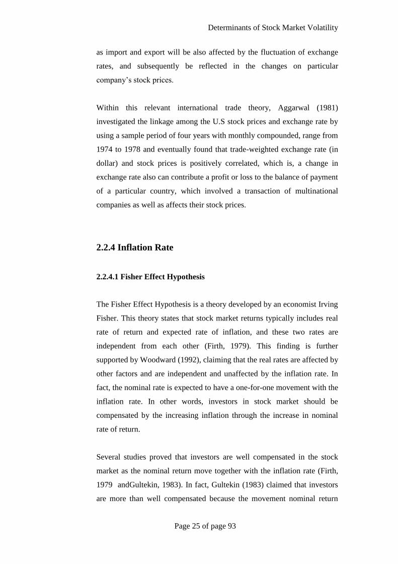
2.2.6 Relevant Theoretical Framework
Schwert (1989) investigated the stock market volatility which involved
macroeconomic variables volatility such as inflation, money growth,
federal fund rate and industrial production. The author also found that the
direction of causality between volatility of return and macroeconomic
variables is not consistent but significant, proving that there is linkage
Determinants of Stock Market Volatility
Page 27 of page 93
between macroeconomic variables and stock market volatility. The
theoretical framework implemented by Schwert (1989) is shown as below:
Figure 2.1 Theoretical Framework By Schwert (1989)
2.3 Proposed Theoretical Framework
Figure 2.2Proposed Theoretical Framework
The proposed theoretical framework for this research is shown above and adapted
partially from Schwert (1989), excluding money growth, including exchange rate.
Stock market volatility
Inflation
Money growth
Federal funds rate
Industrial production
Interest rate
Inflation rate
Exchange rate
Stock market
index
Gross domestic
production growth
rate

Determinants of Stock Market Volatility
Page 28 of page 93
CHAPTER 3: METHODOLOGY
3.0 Introduction
The main objective of chapter 3 is to exhibit the methodology of this study in a
structured and well-organized manner. Necessary data are collected through the
data collection method discussed in this section following the data processing
procedures and econometric model and methods applied. This chapter mainly
consists of the following part: 1) research design, 2) data collection method, 3)
data processing procedures, 4) econometric models and econometric methods.
3.1 Research Design
This research purely uses quantitative data. This research includes one dependent
variable and four macroeconomics variables as independent variables. There are
four independent variables which are interest rates, exchange rate, inflation rate
and gross domestic production. A total of 34 observations used in this research
which is from 1980 to 2013. EViews 6 software has been applied as the method to
determine the relationship between the stock price and the four macroeconomic
variables.
3.2 Data Collection Method
This study focuses on secondary data. This research employed time series data
which extracted from the same database which is Datastream database.

Determinants of Stock Market Volatility
Page 29 of page 93
3.2.1 Secondary Data
This study uses time series data which consist of 34 observations from
1980 to 2013. The dependent variable is FTSE Bursa Malaysia Index. The
four independent variables are interest rate, exchange rate, consumer price
index (CPI) and gross domestic production (GDP) growth rate.
Table 3.1 Data Sources
Variable Proxy Unit
measurement
Description Sources
Stock market
index
KLCI Index Stock market
index in Malaysia
Datastream
Interest rate INT Percentage (%) Government
securities,
Treasury bill rate
(3 months)
Datasttream
Exchange rate EXC Index Exchange rate of
Malaysia Ringgit
(Base rate
2010=100)
Datastream
Consumer price
index
CPI Index Consumer price
index are used as
indicator of
inflation rate in
Malaysia (Base
rate 2010=100)
Datastream
Gross domestic
production
growth rate
GDP Percentage (%) Malaysia GDP
annual growth
rate
Datastream

Determinants of Stock Market Volatility
Page 30 of page 93
3.3 Data Processing Procedures
Figure 3.1 Illustration of Data Processing
In this study, data processing comprises four steps. Firstly, relevant data will be
collected from secondary sources (DataStream). Next, the collected data will be
filtered and rearranged. Then, the data are edited and transformed into useable
form by using statistical tool (E-views). The transformed data are then being
studied and analyzed using statistic tool. Finally, the results generated are ready
for interpretation.
3.4 Econometric Regression Model
Econometric Function
KLCI= f (Interest rate, Inflation rate, GDP growth, Exchange rate)
Expected sign for the selected independent variables
Interest rate: negative
Inflation rate: negative
Gross domestic production growth rate: positive
Exchange rate: positive
1st Step: Collect necessary data from secondary sources (DataStream)
2nd Step: Screen, edit and transform data into useable information
3rd Step: Study and analyze data using statistic tools (E-views)
4th Step: Interpret and explain the results generated
Determinants of Stock Market Volatility
Page 31 of page 93
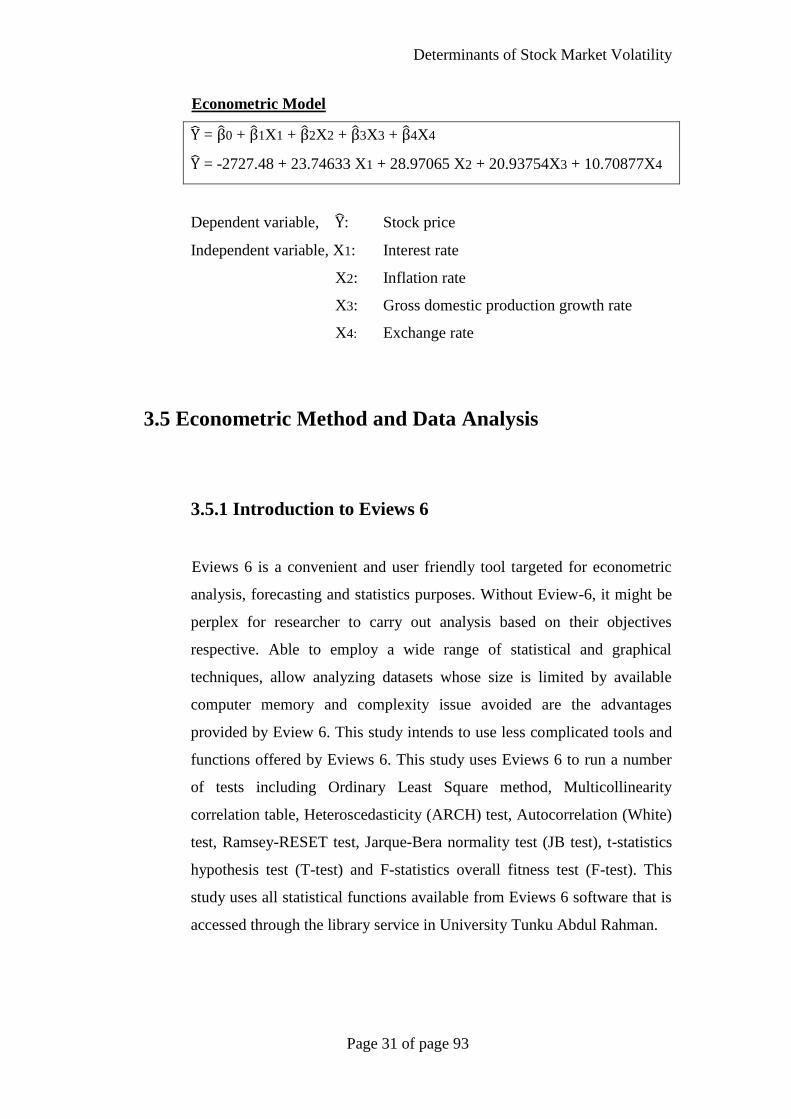
Econometric Model
Y = β0 + β1X1 + β2X2 + β3X3 + β4X4
Y = -2727.48 + 23.74633 X1 + 28.97065 X2 + 20.93754X3 + 10.70877X4
Dependent variable, Y: Stock price
Independent variable, X1: Interest rate
X2: Inflation rate
X3: Gross domestic production growth rate
X4: Exchange rate
3.5 Econometric Method and Data Analysis
3.5.1 Introduction to Eviews 6
Eviews 6 is a convenient and user friendly tool targeted for econometric
analysis, forecasting and statistics purposes. Without Eview-6, it might be
perplex for researcher to carry out analysis based on their objectives
respective. Able to employ a wide range of statistical and graphical
techniques, allow analyzing datasets whose size is limited by available
computer memory and complexity issue avoided are the advantages
provided by Eview 6. This study intends to use less complicated tools and
functions offered by Eviews 6. This study uses Eviews 6 to run a number
of tests including Ordinary Least Square method, Multicollinearity
correlation table, Heteroscedasticity (ARCH) test, Autocorrelation (White)
test, Ramsey-RESET test, Jarque-Bera normality test (JB test), t-statistics
hypothesis test (T-test) and F-statistics overall fitness test (F-test). This
study uses all statistical functions available from Eviews 6 software that is
accessed through the library service in University Tunku Abdul Rahman.

Determinants of Stock Market Volatility
Page 32 of page 93
3.5.2 P-value
P-value is used when performing a hypothesis testing in an analysis or
statistics. Hypothesis tests are basically used to test whether the claim
about a population is valid. Hence, P-value helps to determine the
significance of the results. There are two hypothesis for the claim, which
called the null hypothesis and alternative hypothesis. Null hypothesis is the
claim that is on trial, whereas the alternative hypothesis is the one that
believe to conclude the null hypothesis to be untrue. How to interpret?
When the p-value is not more the α (significance level assume =
0.05), it points to strong evidence against the null hypothesis, thus,
reject null hypothesis.
When the p-value is more than the α (significance level assume =
0.05), it points to weak evidence against the null hypothesis, thus,
do not reject null hypothesis.
Therefore, p-value allows the readers to draw their own conclusion.
3.5.3 T-statistic hypothesis test
T-test helps researcher to compare whether two groups have dissimilar
average values. In layman’s term, whether male and female have different
average score during an exam. The differences between these two groups
happened due to the random probability in the selection of sample. It is
considered to be more accurate and actual if the variances between the
mean is bigger, as well as the sample size, and low standard deviation.
The main output of t-test is the t-test’s statistical significance, which
determines whether the variation between the sample averages is close to
the real variation between the populations.

Determinants of Stock Market Volatility
Page 33 of page 93
Figure 3.2 Normal Distribution Curve
𝑁𝑢𝑙𝑙𝐻𝑦𝑝𝑜𝑡ℎ𝑒𝑠𝑖𝑠: 𝐻0: µ = µ0
𝐴𝑙𝑡𝑒𝑟𝑛𝑎𝑡𝑒𝐻𝑦𝑝𝑜𝑡ℎ𝑒𝑠𝑖𝑠: 𝐻1: µ > µ0
Reject the null hypothesis if F-statistic value is larger than the
critical value at a specific α (significance level assume = 0.05).
Reject the null hypothesis if F-statistic value is lower than the
critical value at a specific α (significance level assume = 0.05).
For two-tailed test, reject the null hypothesis if t-statistic value is
larger than the upper critical value, or less than lower critical value
at a specific significance level (assume = 0.05). Otherwise, do not
reject null hypothesis.
F-test
F-test is different from T-test, where it is a statistical test which used to
indicate whether the normal distribution is having the similar variances or
standard deviation between two populations. In other word, the result will
tell whether the model is significance. It is an essential part for Analysis of
Variance (ANOVA). However, the procedure is still the same as T-test
when carrying out the F-test, which required indicating the level of
significance and resolving the critical value by finding out the degrees of
freedom (d.f) of numerator and denominator.
𝐼𝑓𝐹𝑐𝑎𝑙𝑐𝑢𝑙𝑎𝑡𝑒𝑑 > 𝐹𝑐𝑟𝑖𝑡𝑖𝑐𝑎𝑙 , 𝑁𝑢𝑙𝑙ℎ𝑦𝑝𝑜𝑡ℎ𝑒𝑠𝑖𝑠𝑖𝑠𝑟𝑒𝑗𝑒𝑐𝑡𝑒𝑑.
𝐼𝑓𝐹𝑐𝑎𝑙𝑐𝑢𝑙𝑎𝑡𝑒𝑑 < 𝐹𝑐𝑟𝑖𝑡𝑖𝑐𝑎𝑙 , 𝑁𝑢𝑙𝑙ℎ𝑦𝑝𝑜𝑡ℎ𝑒𝑠𝑖𝑠𝑐𝑎𝑛𝑛𝑜𝑡𝑏𝑒𝑟𝑒𝑗𝑒𝑐𝑡𝑒𝑑.
Reject the null hypothesis if the F-statistic value is larger than
critical value at a specific significance level (assume = 0.05).
Determinants of Stock Market Volatility
Page 34 of page 93
Reject the null hypothesis if the F-statistic value is lower than
critical value at a specific significance level (assume = 0.05).
3.5.4 Multicollinearity
Multicollinearitymeans that the situation of independent variables is
greatly correlated with each other. Besides that, R-Squared can be use for
detection of multicollinearity between the paired independent variables
(Gujarati & Porter, 2009).
Frisch (1934) definedMulticollinearity as a linear relationship among the
independent variables in a particular regression model. In a deeper direct
explanation, multicollinearity refers to more than one relationship among
the variables whereascollinearity refers to a single relationship. However,
multicollinearity refers to both casesin most practices.
According to Montgomery and Elizabeth (1975),there are few factor in the
model will causes multicollinearity happen:
1) The method of collection of data is not fit with the model.
2) Limitation on the population being sample or constraint in the model.
3) Model specification bias.
4) An over-explained model.
5) The independent variable exhibit same trend of pattern overtime.
There are a few ways to detect Multicollinearity in a model. First, a high
R-square or high F statistic and few significantT-statistics will encourage
us to reject the null hypothesis,indicating that the independent variables
are correlated. Second,VIF=1/(1-R2) can compute the condition number.
However, this may not always be useful as the standard errors of the
estimates depend on the ratios of elements of the characteristic vectors to
the roots. High sample correlation coefficients are sufficient but not
necessary for multicollinearity(Gujarati & Porter, 2009).

Determinants of Stock Market Volatility
Page 35 of page 93
There are some effects of Multicollinearity in the model. Firstly, the large
standard errors mean will be large. This may due to small observed test
statistics. Secondly, there will be a tendency for large standard errors of
the estimates. Thirdly, the OLS regression model is still BLUE and
consistent even when multicollinearity exist (Gujarati & Porter, 2009).
3.5.5 Heteroscedasticity
In econometrics, Autoregressive Conditional Heteroscedasticity (ARCH),
which introduced by Engle (1982), is one of the tests that observed
whether a time series model is suffering from heteroscedasticity problem
(Nelson, 1991).To make it simple, one out of nine assumption of Classical
Linear Regression Model stated that the error term should be
homoscedasticity, or equal variances of the error term. Thus,
heteroscedasticity violates the assumption of (CLRM) classical linear
regression model, where the model does not have an equal variance of the
disturbance:
Figure 3.3 Variance of Error Term
𝑬(𝒆𝒊𝟐) = 𝝈𝒊
𝟐
HOMOSCEDASTICITY HETEROSCEDASTICITY
Heteroscedasticity happens for a few reasons. First and foremost, the
model misspecification, which mean an incorrect data or incorrect
functional form for linear model may leads to heteroscedasticity problem.
Secondly, including too much of independent variables might cause more

Determinants of Stock Market Volatility
Page 36 of page 93
error to exist and eventually cause heteroscedasticity problem. Thirdly,
heteroscedasticity also arises with the presence of outlier as it leads to
extrapolation. Also, the incorrect data provided by the respondent will
cause measurement error as well as heteroscedasticity problem. Last but
not least, an extremely positive or negative value in independent variables
also will leads to heteroscedasticity problem.
There are several impact of heteroscedasticity in the disturbances of a
linear model, including unbiased but consistent, and they no longer the
Best Linear Unbiased Efficient (BLUE), hence, the inefficient parameter
estimates would eventually affect the hypothesis to be invalid with the
presence of heteroscedasticity (White, 1980).
There are several tests that can be applied in order for detection whether
there is heteroscedasticity problem exists, such as:
Figure 3.4 Processes to Detect Heteroscedasticity
This study employed the Autoregressive Conditional Heteroscedasticity
(ARCH) because our model is time series data. Firstly, the null hypothesis
states that error term are homoscedasticity, while alternatives hypothesis as
heteroscedasticity. Secondly, this study rejects the null hypothesis by
comparing the p-value and significance level (assume 5%). Reject the null
Detection of Heteroscedasticity
Informal
Nature of problems
Graphical Method
Formal
Park Test
Glesjer Test
Breusch-Pagan Test
White Test
ARCH Test

Determinants of Stock Market Volatility
Page 37 of page 93
hypothesis if the p-value is smaller than the significance level (assume
5%), otherwise, do not reject null hypothesis, which indicate the model
does not suffer from heteroscedasticity problem. It means that the variance
of error term is constant.
Some solving action would have to carry out if any heteroscedasticity
problem has found in the model. For instances, logs can be added into the
dependent or independent variables or re-specifying the model by
transforming the variables in order to reduce the problem.
3.5.6 Autocorrelation
Autocorrelation is mean that the correlation between elements of series of
observation ordered in time series data or in cross sectional data (Kendall
and Buckland,1971)
There are two way to detect auto correlation problem in the model. It can
be find out by using graphical way or running the formal test, example of
the test are:
1. The Durbin Watson Test
2. The Breusch-Godfrey Test
3. The Durbin’s h Test (for the existing of lagged in dependent variables)
4. Engle’s ARCH Test
The following graphs show the model with positive and negative
autocorrelation problem.
Figure 3.5Distribution of Error Term

Determinants of Stock Market Volatility
Page 38 of page 93
Consequence of autocorrelation are first, when the error terms (µ’s) are
seriously correlated then the OLS estimator are unbiased but optimality
property (Minimum variances property) is not satisfy .Second, if the error
term µ’s are autocorrelated then the OLS variance is greater than the
variance of estimate calculated by other method then the usual t and F test
of significance are no longer misleading conclusion about the estimate
regression. Third, if the disturbance terms are autocorrelated then the OLS
estimate are non-asymptotic. Fourth, the variance of random term is may
be seriously under estimated if the µi’s are autocorrelated (Greene,2000)
There are some measure can be taken as a remedial for autocorrelation
problem. First, identify the independent variable that caused the model
tend to be specification bias. Second, generalised least square model or
GLS model can be used to transform the model which have exhibit the
pure correlation problem. Third, if lager sample size can use Newey-West
method to get standard error of OLS estimators that are correlated from
autocorrelation. This method is derivate from whites’
heteroscedasticity(Gujarati & Porter, 2009).
3.6 Conclusion
In the nutshell, this chapter has provided clear explanation on the research design,
data collection and processing methods. Econometric model applied in this study
is also clearly stated in this chapter. Lastly, this chapter also covered and provided
explanation for all econometric methods and statistical test applied in this research.

Determinants of Stock Market Volatility
Page 39 of page 93
CHAPTER 4: DATA ANALYSIS
4.0 Introduction
This chapter highlights the diagnostic checking for this study using various
method including Jarque-Bera normality test (JB test), regression specification test
(Ramsey’s Regression Specification Error Test), Heteroskedasticity Test
(Breusch-Pagan-Godfrey test), Autocorrelation (Breusch-Godfrey Serial
Correlation LM Test) and multicollinearity test. This study uses all tools available
from Eviews 6 to conduct the test for robustness of this study.
4.1 Diagnostic Checking
4.1.1 Jarque-Bera Normality Test (JB Test)
Hypothesis
H0: The error term is normality distributed.
H1: The error term is not normality distributed.
Significance level
α = 0.05
Decision rule
Reject H0 if p-value of Jarque-Bera statistic is less than α = 0.05.
Otherwise, do not reject H0.
Table 4.1 JB Normality Test Output
Jarque-Bera Probability
0.762680 0.682946

Determinants of Stock Market Volatility
Page 40 of page 93
Decision
Do not reject H0 since p-value of Jarque-Bera statistic (0.682946) is more
than significance level (α = 0.05).
Conclusion
There is insufficient evidence to conclude that the error term is not
normally distributed at significance level α = 0.05. Therefore, the model
does not face normality problem.
4.1.2 Regression Specification Test (Ramsey’s Regression
Specification Error Test)
Hypothesis
H0: Model is correctly specified.
H1: Model is incorrectly specified.
Significance level
α = 0.05
Decision rule
Reject H0 if p-value of is less than α = 0.05. Otherwise, do not reject H0.
Table 4.2 Ramsey’s Regression Specification Error Test Output
F- Statistics Probability
0.125810 0.7255
Decision
Do not reject H0 since p-value (0.7255) is more than significance level
(0.05).
Conclusion
There is insufficient evidence to conclude that the model is incorrectly
specified at significance level α = 0.05

Determinants of Stock Market Volatility
Page 41 of page 93
4.1.3 Heteroskedasticity Test (Breusch-Pagan-Godfrey test)
Hypothesis
H0: There is not heteroskedasticity problem.
H1: There is heteroskedasticity problem.
Significance level
α = 0.05
Decision Rule
Reject 𝐻0 if the P-value is smaller than the significance level, α = 0.05.
Otherwise, do not reject H0.
Decision Making
Heteroskedasticity Test: Breusch-Pagan-Godfrey
F-statistic 0.773326 Prob. F(4,29) 0.5515
Obs*R-squared 3.277080 Prob. Chi-Square(4) 0.5126
Scaled explained SS 1.775376 Prob. Chi-Square(4) 0.7770
Since the P-value, 0.5126 is greater than the significance level, α = 0.05,
do not reject H0.
Conclusion
There is insufficient evidence to conclude that there is heteroskedasticity
problem in the model at 5% significance level.

Determinants of Stock Market Volatility
Page 42 of page 93
4.1.4 Autocorrelation (Breusch-Godfrey Serial Correlation
LM Test)
Hypothesis
H0: There is not autocorrelation problem.
H1: There is autocorrelation problem.
Significance level
α = 0.05
Decision Rule
Reject H0 if the p-value is less than the significance level, α = 0.05.
Otherwise, do not reject H0.
Decision Making
Breusch-Godfrey Serial Correlation LM Test:
F-statistic 0.055384 Prob. F(2,27) 0.9462
Obs*R-squared 0.138915 Prob. Chi-Square(2) 0.9329
Since the P-value, 0.9329 is greater than the significance level, α = 0.05,
do not reject H0.
Conclusion
There is insufficient evidence to conclude that there is autocorrelation
problem in the model at 5% significance level.

Determinants of Stock Market Volatility
Page 43 of page 93
4.1.5 Multicollinearity Test
Detection of Multicollinearity (4 Methods)
4.1.5.1 High 𝐑𝟐 but few significant t-ratio
Dependent Variable: KLCI
Method: Least Squares
Date: 06/23/15 Time: 12:07
Sample: 1980 2013
Included observations: 34
Variable Coefficient Std. Error t-Statistic Prob.
INT 23.74633 14.82988 1.601249 0.1202
INF 28.97065 1.693967 17.10225 0.0000
GDP 20.93754 5.662064 3.697863 0.0009
EXC 10.70877 1.661624 6.444760 0.0000
C -2727.480 284.9492 -9.571811 0.0000
R-squared 0.934313 Mean dependent var 794.4709
Adjusted R-squared 0.925253 S.D. dependent var 415.2933
S.E. of regression 113.5407 Akaike info criterion 12.43725
Sum squared resid 373853.3 Schwarz criterion 12.66172
Log likelihood -206.4333 Hannan-Quinn criter. 12.51380
F-statistic 103.1224 Durbin-Watson stat 1.997425
Prob(F-statistic) 0.000000
Interpretation: Our model consists of high R2 which is 0.934313 with a
major of significant t-ratio which is inflation rates, gross domestic product
(GDP), and exchange rate. But only with one insignificant t-ratio which is
interest rates. Thus, this method suggests this model does not suffer from
serious multicollinearity problem.

Determinants of Stock Market Volatility
Page 44 of page 93
4.1.5.2 High pairwise correlation among X’s
Table 4.3 Correlation Analysis
KLCI INT INF GDP EXC
KLCI 1.000000 -0.318710 0.855870 0.106762 -0.421134
INT -0.318710 1.000000 -0.526848 0.188786 0.511867
INF 0.855870 -0.526848 1.000000 -0.219124 -0.785225
GDP 0.106762 0.188786 -0.219124 1.000000 0.370743
EXC -0.421134 0.511867 -0.785225 0.370743 1.000000
Interpretation: Correlation is a method to indicate the relationship between
two quantitative variables. In other words, it is a measurement of the
strength of the association between these two variables. These correlation
ranges from -1 to +1. However, only correlation between Exchange rate
and Inflation rate indicates a strong negative relationship of -0.785225
while other variables remained weak and moderate relationship based on
Pearson’s correlation coefficient range table:
Table 4.4 Pearson’s Correlation Coefficient Range Table
< 0.2 Very weak relationship
0.2 – 0.4 Weak relationship
0.4 – 0.6 Moderate relationship
0.6 – 0.8 Strong relationship
> 0.8 Very strong relationship
4.1.5.3 Variance inflation Factor, VIF = (1/1-𝑹𝒂𝒖𝒙𝟐 )
Decision Rule
There is serious multicollinearity problem if VIF is more than 10.
Otherwise, there is no serious multicollinearity problem.

Determinants of Stock Market Volatility
Page 45 of page 93
Decision Making
Calculating VIF:
Table 4.5 Variance Inflation Factor (VIF)
VARIABLES 𝟏
𝟏 − 𝐑𝐢𝟐
= 𝐕𝐈𝐅
VARIANCE
INFLATION FACTOR
(VIF)
INTEREST RATES 1
1 − 0.303300= 1.435338022 1.44
INFLATION 1
1 − 0.643703= 2.806647263 2.81
EXCHANGE RATES 1
1 − 0.667624= 3.008640816 3.01
GROSS DOMESTIC
PRODUCT
1
1 − 0.151692= 1.178817128 1.18
Conclusion
Base on the VIF calculated, the highest VIF is only 3.01. This indicates
that there is no serious multicollinearity problem among the variables.
4.1.5.4 Tolerance (TOL) factors = (1/VIF)
Table 4.6 Tolerance Factors
VARIABLES TOLERANCE FACTOR (TOL)
INTEREST RATES 1
1.435338022= 0.6967
INFLATION 1
2.806647263= 0.6967
EXCHANGE RATES 1
3.008640816= 0.3324
GROSS DOMESTIC PRODUCT 1
1.178817128= 0.8483

Determinants of Stock Market Volatility
Page 46 of page 93
4.2 Hypothesis testing
4.2.1 Hypothesis for Model Fit (F- Test)
In order to test the overall significance of the estimated regression model,
this research decided to use F- test with P- value at significance level of
0.05 to examine it.
Hypothesis
H0: β1=β2=β3=β4=0
H1: At least one of theβi is not equal to zero, where i = 1,2,3,4
Decision rule
Reject H0, if the p-value is less than the significance level 0.05. Otherwise
we do not reject H0.
Decision making
Reject H0 since the Prob(F- statistic) = 0.000000 is less than the
significance level of 0.05.
Conclusion
There is sufficient evidence to conclude that at least one of the βi is not
equal to zero, where i= 1,2,3,4 at significance level of 0.05. This result
shows that the model is overall significant.
4.2.2 Hypothesis testing (t- test)
In order to test whether each independent variable is significant or not, this
research decided to use t- test with p- value approach at significance level
of 0.05 to examine it.

Determinants of Stock Market Volatility
Page 47 of page 93
Hypothesis
H0= There is no significant relationship between independent variable and
dependent variable.
H1= There is significant relationship between independent variable and
dependent variable.
Decision rule
Reject H0 of the p- value is lesser than the significance level, otherwise do
not reject H0.
4.2.2.1 Interest rate
Hypothesis
H0:β1=0
H1:β1≠0
Decision rule
Reject H0 of the p- value is lesser than the significance level, otherwise do
not reject H0.
Decision Making
Do not reject H0 since the p-value (0.1202) is greater than the significance
level (0.05).
Conclusion
There is insufficient evidence to conclude that β1≠0. This result shows that
there is no significant relationship between interest rate and KLCI stock
market index.

Determinants of Stock Market Volatility
Page 48 of page 93
4.2.2.2 Inflation rate
Hypothesis
H0:β2=0
H1:β2≠0
Decision rule
Reject H0 of the p- value is lesser than the significance level, otherwise do
not reject H0.
Decision Making
Reject H0 since the p-value (0.0000) is lesser than the significance level
(0.05).
Conclusion
There is sufficient evidence to conclude that β2≠0. This result shows that
there is significant relationship between inflation rate and KLCI stock
market index.
4.2.2.3 Gross Domestic Product
Hypothesis
H0:β3=0
H1:β3≠0
Decision rule
Reject H0 of the p- value is lesser than the significance level, otherwise do
not reject H0.
Decision Making
Reject H0 since the p-value (0.0009) is lesser than the significance level
(0.05).

Determinants of Stock Market Volatility
Page 49 of page 93
Conclusion
There is sufficient evidence to conclude that β3≠0. This result shows that
there is significant relationship between Gross Domestic Product and
KLCI stock market index.
4.2.2.4 Exchange rate
Hypothesis
H0:β4=0
H1:β4≠0
Decision rule
Reject H0 of the p- value is lesser than the significance level, otherwise do
not reject H0.
Decision Making
Reject H0 since the p-value (0.0000) is lesser than the significance level
(0.05).
Conclusion
There is sufficient evidence to conclude that β4≠0. This result shows that
there is significant relationship between exchange rate and KLCI stock
market index.
4.3 Interpretation
4.3.1 Parameters interpretation
β1 = 23.74633
When interest rate (INT) increases by 1 percentage point, on average, KLCI
stock index will increased by 23.74633 basis point, holding other variable
constant.

Determinants of Stock Market Volatility
Page 50 of page 93
β2 = 28.97065
When the consumer price index (CPI) increases by one basis point, on
average, KLCI stock market index in Malaysia will increase by 28.97065
basis points, ceteris paribus.
β3 = 20.93754
When the Gross Domestic Product growth (GDP) increases by one percent
point, on average, the stock price index in Malaysia will be increased by
20.93754 basis points, holding other variables constant.
β4 = 10.70877
When the exchange rate index increases by one basis point, on average, KLCI
stock market index in Malaysia will increase by 10.70877 basis points, while
holding other variables constants.
4.3.2 Goodness of fit
R-squared= 0.934313
There are 93.4313% of the total variation in the KLCI stock index can be
explained by the total variation in Interest rate, inflation rate, gross domestic
product and exchange rate.
Adjusted R-squared= 0.925253
There are 92.5253% of the total variation in the KLCI stock index can be
explained by the total variation in Interest rate, inflation rate, gross domestic
product and exchange rate after taking the sample size and degree of freedom
into account.
Determinants of Stock Market Volatility
Page 51 of page 93
4.4 Conclusion
This chapter basically covers five robustness tests which includes testing for
normality problems, model specification errors, multicollinearity among variables,
heteroskedasticity as well as autocorrelation problems. Lastly, this chapter covers
hypothesis t-testing to estimate the parameters of each variable in the regression
model as well as to test the significance of model as a whole.
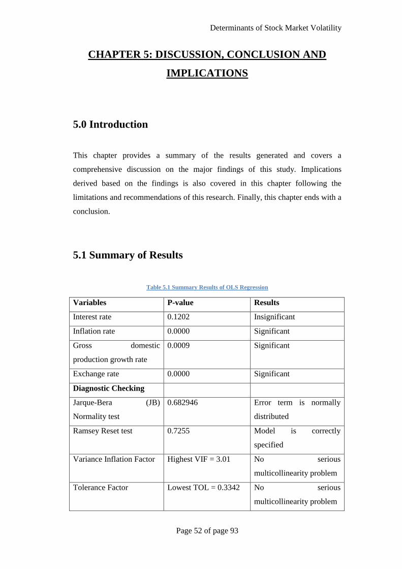
Determinants of Stock Market Volatility
Page 52 of page 93
CHAPTER 5: DISCUSSION, CONCLUSION AND
IMPLICATIONS
5.0 Introduction
This chapter provides a summary of the results generated and covers a
comprehensive discussion on the major findings of this study. Implications
derived based on the findings is also covered in this chapter following the
limitations and recommendations of this research. Finally, this chapter ends with a
conclusion.
5.1 Summary of Results
Table 5.1 Summary Results of OLS Regression
Variables P-value Results
Interest rate 0.1202 Insignificant
Inflation rate 0.0000 Significant
Gross domestic
production growth rate
0.0009 Significant
Exchange rate 0.0000 Significant
Diagnostic Checking
Jarque-Bera (JB)
Normality test
0.682946 Error term is normally
distributed
Ramsey Reset test 0.7255 Model is correctly
specified
Variance Inflation Factor Highest VIF = 3.01 No serious
multicollinearity problem
Tolerance Factor Lowest TOL = 0.3342 No serious
multicollinearity problem

Determinants of Stock Market Volatility
Page 53 of page 93
Breusch-Pagan-Godfrey
Heteroskedasticity test
0.5126 No heteroscedasticity
problem in this model
Breusch-Godfrey Serial
Correlation LM test
0.9329 No autocorrelation
problem in this model
5.2 Discussion of major findings
5.2.0 Expected sign vs. Actual output
Based on the empirical result generated, this research found that only GDP
growth rate and exchange rate have the same sign with what this study
expected. On the other hand, interest rate and inflation rate have the
opposite sign, which is inconsistent with what this study expected.
5.2.1 Interest rate
The interest rate used in this research is 3-month Treasury bill rate issued
by Malaysia government. As T- bill rate is risk free rate and it is the
minimum return that investors required, it is useful to examine how
interest rate will affect stock market index.
This research shows that interest rate positively affect stock market index.
This result is inconsistent with most of the study. The reason is that this
research used 3- month T- bill rate which is different from other researches
which used long term interest rate. Mukherjee and Naka (1995) stated that
although there is an ordinary negative correlation among the market return
and the long-term government bond rate, yet there is a controversial
positive correlation among the short-term call money rate and the return.
Nasseh and Strauss (2000) also supported this view as they found a similar
results which is positive relationship between short- term interest rate and

Determinants of Stock Market Volatility
Page 54 of page 93
stock price but negative relationship between long- term interest rate and
stock price in six European markets.
There are three sectors that will be benefited from a rise of interest rate,
which is consumer discretionary, technology and financial sector.O’Hare,
chief market analyst at Briefing.com reported by Brecht (2015) stated that
the beginning part of a rise in interest rate should be beneficial to the
consumer sector, higher rates are almost certainly the result of an
improvement in economic growth that is an advanced levels of
employment will establish a formidable sense of job security, better wage
growth and a rise of lending activity, which will eventually leads to higher
levels of spending (Brecht, 2015). When individuals have higher wages,
the demand of nonessential goods, luxury goods and investment will
increase. This will improve the company stock price as demand of goods
and service and investment in companies stock is higher.
Financial sector will also benefited from a rise in interest rate as the
interest margin which is the difference between borrowings and lending
cost is higher, this will bring higher profit to the financial sector, in other
words rise in interest rate will bring positive effect to financial sector.
Blain, chief executive officer at New Bern, North Carolina-based BlueSky
Wealth Advisor, reported by Brecht (2015) pointed out that, financial
market are beneficial from the rising of interest rates due to an interest
margin expands, profit raising, and the increased economic activity that
affected the interest rate increase generally means more loan demand.
Tech companies tend to carry low debt load and a stable fixed- capital
structure. This paradigm frequently leads to widening margins when sales
accelerate, which would also leads to a rise in dividends (Wyatt
Investment Research, 2014). As higher interest rates usually indicate
economic growth, it would bring positive effect to technology sector
because the spending in technology goods will increase due to higher
wages and the demand of technology stocks will be higher as it pays out
more dividends which imply that technology corporation is making

Determinants of Stock Market Volatility
Page 55 of page 93
profit.KLCI stock index consists of companies from seven sectors which
are financial, plantation, telecommunications, gaming, utilities, consumers
and transportation sectors. All these sectors are highly related to financial
and consumer spending activities, which will be benefited from a rise in
interest rate. This may be the reason why Malaysia stock market index has
positive relationship with interest rate.
Nevertheless, this research shows that the linkage between stock market
index and interest rate is not significant. The Islamic banking sector in
Malaysia has outperformed conventional banking sector in recent years.
Malaysian Islamic banking sector has average annual asset growth rate of
18.6 percent from 2008 to 2012 compared to the conventional bank growth
of 9.3 percent. In 2013, Malaysia was the largest Sukuk (bond) issuer
which issued 69 percent of total issuance in the world.
Malaysia also has the largest number of funds by domicile which is 28
percent and in term of Islamic funds’ assets by domicile and Malaysia (22
percent) is the second largest Islamic fund market just below Saudi Arabia
(44 percent) (Malaysia International Islamic Financial Centre, 2014). All
these data shows that Malaysia has shifted their focus on mode of finance
from conventional to Islamic in recent years. As Islamic finance prohibits
the use of interest (Riba) and Malaysia has focused more on Islamic
finance rather than conventional finance, interest rate may not have
significant relationship with stock market index.
The development if Islamic financial system is represented by Islamic law,
also known as Shari’ah, which forbid interest (Riba), uncertainty (Gharar),
gambling (Maysir), and promotes risk sharing, profit-sharing, asset-backed
financial transactions, and ethical investment (Shamsuddin, 2014). It is
clear that with the prohibition of interest (Riba), Islamic finance does not
focus on interest as the main source when conducting business, thus stock
market should not have sensitivity towards interest rate. This is supported
by Shamsuddin(2014), who examines the interest rate sensitivity of
Islamic equity of Dow Jones (DJ) Islamic Market Index, has found that

Determinants of Stock Market Volatility
Page 56 of page 93
there volatility or changes in long-term interest rate do not influence DJ
Islamic Market Index, DJ Islamic emerging market and Islamic non-US
market portfolios.
5.2.2 Inflation rate
According to the Fisher effect hypothesis discussed earlier in chapter 2, it
states that nominal interest rates equivalent to the combination of real
interest rate and expected inflation rate. Therefore, for the purpose of
maintaining a balance in that equation, nominal interest rates will increase
when the expected inflation rate increases. This finding is supported by
Firth (1979) in U.S market and Gultekin (1983) in countries other than
U.S.Firth (1979) claimed that the stock market provided some hedge
against inflation in the UK but his findings are in contrast with the work of
other researchers in the U.S.A. On the other hand, Yang and Doong (2004),
Apergis (2003), Abrugi (2008) and Emara (2012) argued that inflation rate
is significant negatively related to stock market return. They explained that
a higher domestic inflation rate may lead to depreciation of home currency
and may encourage foreign investors to withdraw or reduce their
investment in the home market due to higher market uncertainty.
Nevertheless, based on the result generated, this study claims that inflation
rate in Malaysia has significant positive relationship with the Malaysia
stock market, which is in agreement with Gultekin (1983), Firth (1979)
and Adam and Tweneboah (2008).In other words, Malaysian stock market
may provide some degree of hedging towards inflation in Malaysia. In fact,
inflation rate has the most impact on the Malaysia stock market among all
variables. Besides, another possible explanation for the positive linkage
between stock market and inflation in Malaysia is that the inflation rate in
Malaysia is relatively low, less than 10 percent, compared to other country
with negative correlation between inflation rate and stock market with
inflation rate more than 10 percent such as Brazil (Abugri, 2006).

Determinants of Stock Market Volatility
Page 57 of page 93
Moreover, based on the inflation level standards of Henry (2002),
countries with inflation rates less than 10 percent will fall under the low
inflation category. His study claims that country with originally low
inflation rate does not enjoy benefits in terms of an increase in stock
market condition from disinflationary actions. According to addition raw
data obtained from World Bank website, this study found that Malaysia hit
its highest inflation peak of 9.7 percent, which is still considered low by
Henry (2002). This means that Malaysia would not have enjoyed any
improvement in the stock market condition if government take
disinflationary actions given that some authors argued that the relationship
between inflation rate and stock market return is negative.
5.2.3 GDP growth rate
The result of this study shows GDP significant positively affects the stock
market index which means that an increase GDP will increase the stock
price. It is consistent with the result from Noormahayu, Norsilawati,
Zarul&Fauzi(2013) who investigate the elements that determine the stock
market return. Researchers found gross domestic product shows positive
relationship with the stock market in term of long run. In addition,
Christopher et al. (2006) also supported the result by examined stock
market in New Zealand.
In 1985, Malaysia’s GDP growth rate has recorded a -1.12% growth rate
while this cause the KLCI decreases from 353.64 to 285.98. In addition to
that, Malaysia suffers the financial crisis in 1997 and has a -7.36% of GDP
growth rate. While the KLCI decline from 1097.54 to 457.61. The same
condition in 2009, GDP growth with -1.51% leads to a decrease of roughly
160 point. This can be explained by GDP reflect the health of economic of
the nation. When the economy is healthy and growing, the firm will be
affected positively with a better earning. The higher profit would

Determinants of Stock Market Volatility
Page 58 of page 93
encourage investors and firm invests more in stock market. Simultaneously,
a negative growth rate of GDP will have a negative effect on stock market.
In the 11th Malaysia Plan the Malaysian government set the goal of 5-6%
of growth rate in the next five years, based on sustained local demand
(Chin, 2015). This is because the continuous structural change will
enhance the momentum for economic growth, including productivity
advancement and innovation. Therefore gives the economic a boost in the
near future. This will gain further momentum for growth, higher household
income per capital as well as increased welfare of the people of Malaysia.
In other words, the economy of Malaysia will be able to grow at a faster
pace.
In addition to that, this movement may be one of the justifications for the
results of this study which found positive linkage between the equity
market return and the GDP growth rate in Malaysia. Normally, economists
look at GDP to measure economic growth. The findings of this study is
supported by Chin (2015) whom implied that productivity advancement by
improved capital efficiency and the contribution of multi-factor
productivity (MFP) productivity from multiple inputs will be important for
the nation’s economic and financial growth. According to the findings of
this study, the stock market in Malaysia will benefit from the improvement
of productivity of the country. This finding is consistence with
Kalyanaraman and Tuwajri (2014) that increase in Malaysia’s GDP can
affect the company earning eventually give a positive impact to the stock
market.
5.2.4 Exchange rate
This study investigates whether the exchange rate has affected the stock
index in Malaysia. While literature suggests that the actuality of significant

Determinants of Stock Market Volatility
Page 59 of page 93
interactions between them, the empirical results provides that exchange
rates is significance to the stock index.
The results of this study found that exchange rate is positive correlated
with the stock market index, which is in the same line with the literature
review discussed in chapter 2, evidence from United States and Australia
by Phylaktis and Ravazzolo (2005), Aggrawal (1981), Richards, Simpson
and Evans (2009). This means that, an increase in exchange rates would
lead to a rise in stock market index.
First and foremost, this relationship could be explained by using demand
and supply theory, where the changes of the currency value would affect
the volume international trade (Hooper and Kohlhagen, 1978) and
eventually affect the nation’s stock index (Huang, Nakamor and Wang,
2005). When a buyer in a country demand goods and services from seller
in another country, is it necessary for the buyer to enter into foreign
exchange market first, in order to buy that particular country’s currency,
before proceed to purchase the foreign products. For instances, assume that
Malaysia has a strong Ringgit Malaysia, and the Ringgit Malaysia is very
valuable compared to other currencies. With this opportunity, Malaysia
could increase their import due to lower prices, and offer these foreign
goods to the customer at lower prices which eventually increase the
quantity demanded for these products. These would probably increase our
profits; consequently, the profits would leads to the growth of the nation’s
stock index.
Figure 5.1Relationship Between Exchange Rate and Stock Market Index
Another possible explanation for the relationship between exchange rate
and stock market is the dependency of the nation’s commodities revenue
income. Based on the Malaysian news, the person in charge of economic
planning, The Malaysian Insider (2015) reported that Datuk Seri Abdul
Strong Malaysia Currency
(MYR)
Increase import of raw material due
to lower prices
Sell with lower cost and gain profits
Leads to a rise in
Malaysia Stock Market
Index

Determinants of Stock Market Volatility
Page 60 of page 93
Wahid Omar claimed that Malaysia is too dependent on oil industry in the
sense of contribution to national income. Theoretically, there is a strong
correlation between the commodities and the exchange rates if a country is
more dependent on a primary domestic industry. This has supported by
Fong (2006), which the author has stated that the commodity price
movements will be associated with the exchange rates if and only if a
country’s export has involved major of that specific commodities. In other
words, the commodity price movement is sensitive to the strength of the
particular currencies (Fong, 2006).
Recently, Liau and Chong (2014) from Bloomberg have reported a news
regarding the stock slump and exposed a risk to crude oil revenues on the
1st of December 2014. They said that after the dropped of the Malaysia
ringgit (MYR) amount to 2.5 percent in two days, the Malaysia KLCI
Index of shares fell 2.3 percent, mostly was dragged down by gas, oil and
plantation stocks. This shows that the relationship between exchange rates
and stock index is positively correlated even after taking the correlation
between commodities price and currency value into account.
Besides, foreign direct investments (FDI) also act as an important role in
between the relationship among exchange rates and stock index. Investors
tend to invest more in countries with strong and stable currency value in
order to safeguard their capital while earning income that is less subjected
to inflation risk. Hence, a strong currency will eventually lead to a better
performing stock market by attracting foreign direct investments to
stimulate growth and expand domestic business in the country.

Determinants of Stock Market Volatility
Page 61 of page 93
5.3 Implications of this study
5.3.1 Interest rate
5.3.1.1 Policy Makers
When implementing monetary policy, policy makers should take into account
the effectiveness of interest rate in affect Malaysia stock market. This study
found positive yet insignificant relationship between interest rate and stock
market. Hence, it is important for policy makers to know that interest rate
may not be the most effective tools to stimulate the Malaysia stock market.
5.3.1.2 Economist and Researchers
The result shows that interest rate is positively and insignificantly affects
stock market is inconsistent with most of the studies, which stated that
interest rate has negative relationship and significantly affects stock market.
This implies that when doing research, researchers need to determine whether
the specific country is Islamic finance-oriented or conventional finance-
oriented as this will bring effect to the result of studies.
5.3.1.3 Market Investors
Investors need to have sufficient knowledge of conventional or Islamic
finance when making investment in securities, as there is some difference
between the way conventional and Islamic conduct business.The main
difference is prohibition and allowance of interest. This makes a huge
difference as changes in interest rate will have immediate effect on investors’
portfolio value. By having sufficient knowledge investors can protect
themselves from the fluctuation of interest rates.
Determinants of Stock Market Volatility
Page 62 of page 93
5.3.1.4 Corporate Management Teams
Although normally an increase in interest rate would bring negative influence
to a corporation as the cost of capital of a corporation will be higher, but
when there is a rise in interest, there is usually an economic growth which
could bring positive effects to company that produce consumer discretionary,
financial product or services and technology product. This benefit may
outperform the negative effect and bring positive effect to corporation when
there is a rise in interest rate.
5.3.2 Inflation rate
5.3.2.1 Policy Makers
The results of this study may be used by policy makers when making
economic policy decisions to prevent causing a crash in the stock market.
Policy makers in Malaysia may have to take into account the fluctuations in
stock market return when controlling the overall price of goods in Malaysia
since the stock market is correlated with the movement of inflation in
Malaysia. Hence, Malaysia policy makers can implement inflation rate
stabilization efforts when they wish to maintain a stable stock market. This
study also suggests that increasing inflation rate may provide certain benefits
such as an increase in the stock market return. However, policy makers
should also consider the impact of fluctuation upon the stock market when
inflation rate is not controlled properly.
5.3.2.2 Market investors
Results in this study suggest that inflation rate is significant and positively
related to stock market return. In order words, investors may be able to hedge
against inflation risk by investing in Malaysia stock market. This study
implies that investing in Malaysia stock market is one of the possible methods
to provide stability in the purchasing power in the event of increasing

Determinants of Stock Market Volatility
Page 63 of page 93
inflation rate. Hence, investing in Malaysia stock market may serve as an
efficient channel to store monetary value and prevent loss in purchasing
power.
5.3.2.3 Corporate Management Teams
The results of this study also provide some implications to corporate and
firms with shares listed on Bursa Malaysia. Assuming Malaysia stock market
is very efficient; the stock price reflects the future expectations and conditions
of a company. Normally, steady increase in inflation rate is a sign of growing
economy. Hence, company that wishes to raise funds in countries with
increasing inflation rate but at the same time wishes to attract investors may
look for countries with steady increasing trend in inflation rate. By doing so,
the corporate may provide a higher possibility of increasing stock return to
hedge against the inflation rate risk and at the same time maintain its stock
price stability. This will help the corporate to gain more certainty over its
stock return to investor and in turn attract more investors.
5.3.3 GDP growth rate
5.3.3.1 Policy Makers
Based on this study, policy makers may want to take into consideration the
GDP growth rate to prevent a market crash such as during the Asian Financial
Crisis in 1997 and 2008 Global Financial Crisis. It is an important note to
policy makers that not only the amount of GDP is important but also the
growth rate. A slowing down growth rate may impose negative impact on
Malaysia stock market and may lead to various stock market troubles.

Determinants of Stock Market Volatility
Page 64 of page 93
5.3.3.2 Economist and Researchers
In general, higher GDP will lead to a better performing stock market.
However, this study suggests that the greater the growth rate, the better the
performance of Malaysia stock market. Not only the volume of GDP but also
the speed of improvement in GDP may bring benefits to Malaysia stock
market. Hence, economist may be able to improve Malaysia stock market by
identifying what factors contribute most to the growth of GDP. In addition to
that, market researchers may be able to boost Malaysia economy by
identifying and developing potential and new market sector in Malaysia.
5.3.3.3 Market investors
Current GDP growth rate reflects the current condition and moving pace of
Malaysia economy. Hence, Investors may study and analyze the current
situation of Malaysia before making an investment in Malaysia stock market.
Malaysian investors may be able to reduce investment risk by having a clear
understand knowledge about the current condition as well as the future
aspects of Malaysia economy which can be reflected through the growth rate
of GDP. Besides, foreign investors may also gain higher return by investing
in a market that possesses high growth rate in which is reflected by high GDP
growth rate. More importantly, international investors may be able to reduce
the market risk in their portfolio by taking into account the current market and
economy condition of the target country because this study found positive
relationship between GDP growth rate and stock market return.
5.3.3.4 Small and Medium Enterprise
SMEs act as an important role in contributing to the GDP of a nation. The
development of human capital and the management capability is crucial for
the performance of the SMEs firm in order to expand the contribution to
Malaysia’s GDP. SMEs may utilize the support given by the government

Determinants of Stock Market Volatility
Page 65 of page 93
fully to strengthen their management skills, financial and learning capacities
in order to contribute more to Malaysia’s GDP. In turn, SMEs that are listed
on Bursa Malaysia may find favour in their stock performances when the
GDP in Malaysia is doing well. SMEs may also focus on productivity instead
of being solely profit-oriented because an increase in the productivity of
Malaysia may provide favourable movements in the stock performance in
Malaysia.
5.3.4 Exchange rate
5.3.4.1 Policy Makers
Considering the impact of heavy reliance on specific sources of income,
Malaysian government may diversify its income from various sources. By
doing so, Malaysian government may reduce the impact of Ringgit currency
fluctuations when Malaysia suffers from the fall of oil prices, which later will
cause the stock market to decline. For example, Malaysian government may
want to develop and nourish sectors such as banking, tourism, construction
and services to diversify its income sources. Besides, by doing so, it can help
to accommodate the losses from oil and gas sector (Kamari, 2015). The Prime
Minister’s Department Datuk Seri Abdul Wahid Omar also says that, soon the
Malaysia’s oil and gas revenue dependency will be reduce to 22 percent in
2015 from 31 percent in 2014 (The Malaysian Insider, 2015).
In addition to that, this study has proven that the nation’s exchange rate is
move in the same way as the nation’s stock market. Therefore, it is an
important decision for the Malaysia Government to choose whether should
imply fixed exchange rate or remain it to be floated in order to sustain the
value of the Malaysia Ringgit. For instances, in the past, former Prime
Minister Tun Dr Mahathir Mohamad once has pegged Malaysia Ringgit for
almost five years despite the Asian financial crisis in 1998 in order to
maintain and control the value of the currency against depreciation. However,
Determinants of Stock Market Volatility
Page 66 of page 93
a common thing that the Malaysia Government need to take note is, pegging
exchange rates require huge amounts of the country’s reserve for the
Malaysia Government to buy or sell the local currency constantly.
Nevertheless, this may provide more certainty and stability for the stock
market in Malaysia in which will be more appealing for investors including
foreign investors.
5.3.4.2 Economist and Researchers
When conducting the research, it is crucial for the economist and researcher
to identify the currency movement from different country because various
countries may have different policy and issues that might act as one of the
factor affecting the fluctuation of exchange rates. Hence, the effect of
movement of exchange rates towards the fluctuation of stock market from
different country can be measure accurately.
5.3.4.3 Market Investors
It is better for the foreign market investor to identify and perform some
analysis such as fundamental or technical analysis to get sufficient
information and knowledge regarding the movement of exchange rates before
participating into it. This is to ensure that the investor could minimize the risk
of losses to a certain desire level of risk based on different investor’s
perspective. Besides, investors may reduce risk by analyzing any situation in
which may affect exchange rate fluctuation to be able to anticipate any
movement in the stock market.
5.3.4.4 Corporate Management Teams
The multinational firm would need to be more concern on the movement of
currency in the market due to the reason that their business transaction is

Determinants of Stock Market Volatility
Page 67 of page 93
strongly related with the fluctuation of exchange rates. If this issue cannot be
well taken care, it could leads to a loss of the multinational firm because of
foreign exchange risk and eventually causes the stock market to fall. In
addition to that, manufacturing firms may find it favourable during an
increase in the local currency value due to lower raw material purchase cost.
Hence, this may send off false signals indicating an increase in efficiency and
effectiveness while the actual reason for the good performance is purely due
to currency exchange effect and may only be temporal.
5.4 Limitations of this study
5.4.1 Stock Index Restrictions
The stock market index used in this research is FTSE Bursa Malaysia
KLCI index which consists of 30 largest companies in FTSE Bursa
Malaysia Emas Index (FBMEMAS) by full market capitalization.
FBMEMAS is the constituents of the FTSE Bursa Malaysia Top 100 index
and FTSE Bursa Malaysia Small Cap Index (FTSE Bursa Malaysia Index
Series, n.d.). This indicates that KLCI index includes companies that is
Shariah compliant and non- Shariah compliant companies, in other words
KLCI index does not exclude Shariah compliant companies. This is the
limitation of this research as this research found that independent variable
interest rate will not have any effect on Islamic index nor Islamic product,
in essence the effect of interest on KLCI index cannot be captured
accurately as it includes both Shariah compliant and non- compliant
companies.

Determinants of Stock Market Volatility
Page 68 of page 93
5.4.2 Debatable sample size
This study consists of only 34 sample size. One of the reasons that this
study did not include a larger sample is due to the restraint of the
methodology. This study employed the Ordinary Least Square method in
estimating the parameters and significance of the selected macro-economic
variables. This study runs the risk of having autocorrelation and
heteroscedasticity problem if sample size is too big. Besides, this paper is
only limited to analyzing the linkage between the selected macroeconomic
variables and Malaysia stock market in a general sense unlike the others,
which studied the relationships in difference ways such as long-term,
short-term, unidirectional or bidirectional effects and requires a larger
sample size of more than 100. However, the results from this study have
proven its robustness through several diagnostic checking procedures and
are found to be free from autocorrelation, heteroskedasticity and serious
multicorrelation problem.
5.4.3 Limitations of linear regression method
Linear regression method technically is not the best model specification
choice when considering “linear” relationships between the independent
and dependent variables, since in reality there are no such optimal
situations (Dowling and Reinke, 2008). In ecology, there are seldom
situation when the data is modelled adequately by regression model, which
have to fulfilled a whole series of assumptions, including normality,
homoscedasticity, fixed X (explanatory variables), independence, and no
model specification bias. The problem arises when all the assumption is
violated, because the model need be rejected (Schneider, Hommel and
Blettner, 2010). Secondly, linear regression method also creates a problem
when considering modelling a non-linear relationships variable.

Determinants of Stock Market Volatility
Page 69 of page 93
5.4.4 Findings is subjected to Malaysia only
The results generated and implication of this study is exclusively for
Malaysia only. This is because all data and information gathered are from
Malaysia. In addition to that, findings of this study may not be similar to
findings of previous studies due to its nature diversity from other countries
such as interest rate structure and exchange rate structure. Besides, the
findings of this study may not be applicable to countries with difference
culture and investor behaviour
5.5 Recommendations for future research
5.5.1 Substitution of FTSE stock index
Interest rate will have significant impact on conventional finance- oriented
countries rather than Islamic finance- oriented countries. Also, interest rate
will not affect stock market index that only consist of companies that are
complying with Shari’ah law. To capture the relationship and effect
between interest rates and stock market index more accurately, future
researchers are recommended to indicate the mode of finance of the
countries and the stock market index that they want to use. Further studies
can use FTSE Bursa Malaysia HidhrahShari’ah index to give more robust
result.
5.5.2 Conduct further research in different countries with
dual financial system
This study encourages future researchers to extend this study into various
stock markets globally to gain a better understanding on the impacts of the
selected macro-economic variables on the stock market, especially interest

Determinants of Stock Market Volatility
Page 70 of page 93
rate. However, one should always be aware of the differences in terms on
nature, culture, structure and behaviour of the government, citizens and
country as it has proven to be an essential role in determining the
relationships and impact of the variables on the stock market. In addition
to that, this study recommends future research to be conducted in countries
similar to Malaysia such that it has the elements of both conventional and
Islamic banking to gain a better understanding on the impact of interest
rate on stock market return.
5.6 Conclusion
This chapter provides a summary for the results generated and includes a
comprehensive discussion of each independent variables base on the results
generated. Furthermore, this chapter offers several implications for each variable
towards a variety of participants. Lastly, this chapter addresses the limitations of
this study following suggestion to overcome it in future research.

Determinants of Stock Market Volatility
Page 71 of page 93
REFERENCES
A brief history of the stock market.(n.d.). Retrieved from http://stock-
market.laws.com/stock-market-history
Abugri, B. A. (2006). Empirical relationship between macroeconomic volatility
and stock returns: Evidence from Latin American Markets. International
Review of Financial Analysis, 17, 396-410.
Abugri, B. A. (2008). Empirical relationship between macroeconomic volatility
and stock returns: Evidence from Latin American markets. International
Review of Financial Analysis, 17(2), 396-410.
Adam. A. M. & Tweneboah. G. (2008). Macroeconomic factors and stock market
movement: Evidence from Ghana. MPRA Paper No.11256, Munich,
Munich Personal RePEc Archives.
Aggarwal, R. (1981). Exchange Rates and Stock Prices: A Study of the U.S.
Capital Markets Under Floating Exchange Rates. Akron Business And
Economic Review,7-12.
Aitken, B. (1998). Have institutional investors destabilized emerging markets?
Contemporary Economic Policy, 16(2), 173-184.
Alam, M. M., & Uddin, M. G. S. (2009). Relationship between interest rate and
stock price: empirical evidence from developed and developing countries.
International journal of business and management, 4(3), 43.
Ang, B. J., & McKibbin, W. J. (2005). Financial liberalization, financial sector
development and growth: Evidence from Malaysia. Journal of
Development Economics, 84(1), 215-233.
Apergis, N. (2003). Inflation, output growth, volatility and causality: evidence
from panel data and the G7 countries. Economics Letters, 83(2), 185-191.
Arbitrage Priceing Theory- APT. (n.d.). Retrieved
fromhttp://www.investopedia.com/terms/a/apt.asp

Determinants of Stock Market Volatility
Page 72 of page 93
Arestis, P., & Demetriades, P. (1997). Financial development and economic
growth: Assessing the evidence*. The Economic Journal, 107(442), 783-
799.
Asgharian. H., Christiansen. C.,& Hou. A. J. (2015). Effects of macroeconomic
uncertainty on the stock and bond markets.Finance Research Letters, 13,
10-16.
Azevedo, A., Karim, M., Gregoriou, A., & Rhodes, M. (2014). Stock price and
volume effects associated with changes in the composition of the FTSE
Bursa Malaysian KLCI. Journal of International Financial Markets,
Institutions and Money, 28, 20-35.
Bai, Z. (2014). Study on the impact of inflation on the stock market in China,
International Journal of Business and Social Science, 5(7), 261-271
Beattire, A. (n.d.). The birth of stock exchange. Retrieved
fromhttp://www.investopedia.com/articles/07/stock-exchange-history.asp
Beetsma, R., & Giuliodori, M. (2012). The changing macroeconomic response to
stock market volatility shocks. Journal of Macroeconomics, 34(2), 281-
293.
Beltratti, A., &Morana, C. (2006). Breaks and persistency: macroeconomic causes
of stock market volatility. Journal of econometrics, 131(1), 151-177.
Bernama. (2014 November 17). MITI to increase SME market growth and GDP
contribution.Free Malaysia Today. Retrieved from:
http://www.freemalaysiatoday.com/category/nation/2014/11/17/miti-to-
increase-sme-market growth-and-gdp-contribution/
Bernanke, B. S., &Kuttner, K. N. (2005). What explains the stock market’s
reaction toFederal Reserve Policy? Journal of Finance, 60, 1221-1257.
Bloomenthal, A. (n. d.). These Sectors benefit from rising interest rate. Retrieved
from http://www.investopedia.com/articles/investing/052814/these-
sectors-benefit-rising- interest-rates.asp

Determinants of Stock Market Volatility
Page 73 of page 93
Brecht, K. (2015). 3 sectors that could benefit from rising interest rate.Retrieved
from http://money.usnews.com/money/personal-finance/mutual-
funds/articles/2015/04/07/3-sectors-that-could-benefit-from-rising-interest-
rates
Caporale, G. M., Hunter, J., & Ali, F. M. (2014). On the linkages between stock
prices and exchange rates: Evidence from the banking crisis of 2007–
2010. International Review of Financial Analysis, 33, 87-103.
Carmichael. B. (1985).Anticipated inflation and the stock market.The Canadian
Journal of Economics, 18(2), 285-293.
Chin (2015). 11th Malaysia Plan: GDP to grow 5% to 6% per annum.The
Star.Retrieved from:http://www.thestar.com.my/Business/Business-
News/2015/05/21/11th-Malaysia-Plan-GDP-growth/?style=biz
Choi, J. J., Elyasiani, E., & Kopecky, K. J. (1992). The sensitivity of bank stock
returns to market interest and exchange rate risks. Journal of Banking
Finance, 16, 983-1004.
Cole, H. L., & Obstfeld, M. (1991). Commodity trade and international risk
sharing: How much do financial markets matter? Journal of Monetary
Economics, 28(1), 3-24.
Cook, T. Q., & Hahn, T. K. (1988). The information content of discount rate
announcements and their effect on market interest rates.Journal of Money,
Credit, and Banking, 20(2), 167-180.
Corradi, V., Distaso, W., &Mele, A. (2013).Macroeconomic determinants of stock
volatility and volatility premiums. Journal of Monetary Economics, 60(2),
203-220.
del Camino Torrecillas, M., &Jareño, F. (2013). Inflation news impact on stock
market: A Review. Pensee, 75(11), 414-419.
Dividend Discount Model. (n.d.). Retrieved from
http://www.investopedia.com/terms/d/ddm.asp

Determinants of Stock Market Volatility
Page 74 of page 93
Docs.statwing.com. (2015).T-Test (Independent Samples) Example and Definition.
Retrieved from http://docs.statwing.com/examples-and-definitions/t-test/
Döpke, J., Pierdzioch, C, & Hartmann, D. (2008).Forecasting stock market
volatility with macroeconomic variables in real time.Journal of Economics
and Business, 60(3), 256-276.
Dornbusch, R., & Fischer, S. (1980). Exchange rates and the current account.The
American Economic Review, 70(5), 960-971.
Dowling, R., Flannery, A., Landis, B., Petritsch, T., Rouphail, N., & Ryus, P.
(2008).Multimodal level of service for urban streets. Transportation
Research Record: Journal of the Transportation Research Board, (2071),
1-7.
Dowling, R. G., & Reinke, D. (2008).Multimodal Level of Service Analysis for
Urban Streets.Washington, United States: Transportation Research Board.
Dummies.com. (2015). What a p-Value Tells You about Statistical Data - For
Dummies. Retrieved from http://www.dummies.com/how-to/content/what-
a-pvalue-tells-you-about-statistical-data.html
Elyasiani, E., & Mansur, I. (1998). Sensitivity of the bank stock returns
distribution to changes in the level and volatility of interest rates: a
GARCH-M model. Journal of Banking Finance, 22(5), 535-563.
Emara, N. (2012). Inflation volatility, institutions and economic growth. Global
Journal of Emrging Market Economies, 4(1), 29-53.
Eviews.com. (2015). EViews 6 Student Version. Retrieved from
http://www.eviews.com/eviews6/eviews6s/evstud6.html
Ezren Zeffirelli, Z. (1995). Performance of the stock market (KLSE) with the
fluctuation of Kuala Lumpur Inter Bank offer rates (KLIBOR).
UniversitiTeknologi MARA
Fama, E. F. (1981). Stock returns, real activity, inflation, and money. The
American Economic Review, 71(4), 545-565.

Determinants of Stock Market Volatility
Page 75 of page 93
Feldstein, M. (1980).Inflation and the Stock Market.The American Economic
Review, 70(5), 839-847.
Firth.M. (1979).The relationship between stock market returns and rates of
inflation.The Journal of Finance, 34(3), 743-749.
Flannery, M. J., & James, C. M. (1984). The effect of interest rate changes on the
common stock returns of financial institutions, Journal of Finance, 39,
1141-1153.
Foerster, S. R., & Sapp, S. G. (2011). Back to fundamentals: The role of expected
cash flows in equity valuation. North American Journal of Economics and
Finance,22, 320-343.
Fong, F. (2006). Determinants of the Canada-US Exchange Rate: From
Commodities to Current Account. Western Undergraduate Economics
Review, 7-14.
French, k. R., Schwert, G. W., &Stambaugh, R. E. (1987).Expected stock returns
and volatility.Journal of Finance Economics, 19, 3-29.
Friedman. M. (1968).The role of monetary policy.The American Economic Review,
57(1), 1-17.
Frisch, R. (1934). Statistical confluence analysis by means of complete regression
systems.Oslo University Institute of Economics, 77(2), 160-163.
FTSE Bursa Malaysia KLCI 30 component stocks. (n. d.). Retrieved from
http://bursa-malaysia.blogspot.com/2009/06/ftse-bursa-malaysia-klci-30-
component.html
FTSE. (n.d.). FTSE Bursa Malaysia Index Series. Retrieved from
http://www.ftse.com/products/indices/bursa-malaysia
Gan, C., Lee, M., Yong, H. H. A., & Zhang, J. (2006). Macroeconomic variables
and stock market interactions: New Zealand evidence. Investment
Management and Financial Innovations, 3(4), 89-101.

Determinants of Stock Market Volatility
Page 76 of page 93
Goh, S. K., & McNown, R. (2015).Examining the exchange rate regime–monetary
policy autonomy nexus: Evidence from Malaysia. International Review of
Economics & Finance, 35, 292-303.
Greene, W. H. (2003). Econometric analysis. New Jersey, United States: Pearson
Education LTD.
Gultekin. N. B. (1983). Stock market returns and inflation forecasts. The Journal
of Finance, 38(3), 663-673.
Gultekin. N. B. (1983). Stock market returns and inflation: Evidence from other
countries. The Journal of Finance, 38(1), 49-65.
Gujarati, D. N., & Porter, D. (2009). Basic Econometrics. New York, United
States: McGraw-Hill. Inc.
Henry. P. B. (2002). Is Disinflation Good for the Stock Market.The Journal of
Finance, 57(4), 1617-1648.
Hooper, P., & Kohlhagen, S. W. (1978).The effect of exchange rate uncertainty on
the prices and volume of international trade. Journal of International
Economics, 8(4), 483-511.
How is the value of the S&P 500 calculated. (n.d.). Retrieved
fromhttp://www.investopedia.com/ask/answers/05/sp500calculation.asp
Huang, W., Nakamori, Y., & Wang, S. Y. (2005).Forecasting stock market
movement direction with support vector machine. Computers &
Operations Research, 32(10), 2513-2522.
Hussin, M., Yahya, M., Muhammad, F., & Awang, S. A. (2012). Macroeconomic
variables and Malaysian Islamic stock market: a time series analysis. The
Journal of Business Studies Quarterly (JBSQ), 3(4), 1-13.
Ibrahim, M. H., & Aziz, H. (2003). Macroeconomic variables and the Malaysian
equity market: a view through rolling subsamples. Journal of economic
studies, 30(1), 6-27.

Determinants of Stock Market Volatility
Page 77 of page 93
Imdadullah, M. (2012). Introduction, Reasons and Consequences of
Heteroscedasticity. Basic Statistics and Data Analysis. Retrieved from
http://itfeature.com/correlation-and- regression-analysis/introduction-
reasons-and-consequences-of-heteroscedasticity
Iqbal, J., & Haider, A. (2005). Arbitrage Pricing Theory: Evidence from an
Emerging Stock Market. The Lahore Journal of Economies, 10(1), 123-
139.
Isaac, O. A., Adedeji, A. A., & Ismail, I. R. (2012). Polynomial Regression
Model of Making Cost Prediction In Mixed Cost Analysis. Mathematical
Theory and Modeling, 2(2), 14-23.
Jones, C. I. (2002). Introduction to economic growth.New York: W. W. Norton
and Co.
Kamari, E. (2015). Oil Prices, Government Revenue And Malaysia’s Economy –
Pt 1. The Establishment Post. Retrieved from
http://www.establishmentpost.com/oil- prices-government-revenue-
malaysias-economy-pt-1/
Kar, M., Nazlıoğlu, S., & Ağır, H. (2010). Financial development and economic
growth nexus in the MENA countries: Bootstrap panel granger causality
analysis. Economic Modelling, 28, 685-693.
Kelsey, D., & Yalcin, E. (2007).The arbitrage pricing theorem with incomplete
preferences.Mathematical Social Sciences, 54, 90-105.
Kendall, M. G., & Buckland, W. R. (1957).A dictionary of statistical terms.A
dictionary of statistical terms.
Kit, Y. B. (n.d.). Malaysia woos sukuk trade. Retrieved from
http://www.ifre.com/malaysia-woos-sukuk-trade/1518935.fullarticle
Korkeamaki, T. (2011). Interest rate sensitivity of the European stock markets
before and after the euro introduction. Journal of International Financial
Markets, Institutions & Money, 21, 811-831.

Determinants of Stock Market Volatility
Page 78 of page 93
Kalyanaraman, L., & Al Tuwajri, B. (2014). Macroeconomic forces and stock
prices: some empirical evidence from Saudi Arabia. International Journal
of Financial Research, 5(1), 81-92.
Lastrapes, W. D., & Koray, F. (1990). International transmission of aggregate
shocks under fixed and flexible exchange rate regimes: United Kingdom,
France and Germany, 1959-1985. Journal of International Money and
Finance, 9, 402-423.
Lewis Jr., R. E. (1955). The theory of Economic Growth.London, England:
George Allen and Unwin.
Liang, Q., & Teng, J. Z. (2005). Financial development and economic growth:
Evidence from China. China Economic Review, 17, 395-411.
Liau, Y., & Choong, E. (2014).Ringgit Slides With Stocks as Oil Slump Poses Risk
to Revenues. Retrieved from
http://www.bloomberg.com/news/articles/2014-12-01/ringgit-set-for-
biggest-two-day-drop-since-1998-on-oil-decline
Mahmudul, A., & Gazi Salah, U. (2009). The relationship between interest rate
and stockprice: Empirical evidence from developed and developing
countries. International Journal of Business and Management, 4(3), 43-51.
Malaysia International Islamic Financial Centre.(2014). MIFC Insights Report.
Retrieved from
http://www.mifc.com/?ch=28&pg=72&ac=62&bb=uploadpdf
Maskay, B., & Chapman, M. (2007).Analyzing the relationship between change in
Money Supply and Stock Market Prices. Illinois Wesleyan University
Economics Department.
Maysami, R. C., Howe, L. C., & Hamzah, M. A. (2004). Relationship
betweenmacroeconomic variables and stock market indices: cointegration
evidence from stock exchange of Singapore’s all-S sector
indices. JurnalPengurusan, 24(1), 47-77.
MBA Skool-Study.Learn.Share.(2015). F-Test Definition | Statistics Dictionary |
MBA Skool-Study.Learn.Share. Retrieved from
http://www.mbaskool.com/business concepts/statistics/8633-f-test.html

Determinants of Stock Market Volatility
Page 79 of page 93
McMillin, W. D. (1991). The velocity of M1 in the 1980s: Evidence from
multivariate time series model. Southern Economic Journal, 57, 34-48.
Montgomery, D. C., Peck, E. A., & Vining, G. G. (2012).Introduction to linear
regression analysis: John Wiley & Sons.
Moya-Martinez, P., Ferrer-Lapena, R., & Escrbano-Sotos, F. (2014). Interest
ratechanges and stock return in Spain: A wavelet analysis. BRQ Business
Research Quartely, 1-16.
Mukherjee, T. K., & Naka, A. (1995). Dynamic relations between macroeconomic
variables and the Japanese stock market: an application of a vector error
correction model. Journal of Financial Research, 18, 223-237.
Murtagh, F., Strack, J. L., & Renaud, O. (2004).On neuro-wavelet
modelling.Decision Support Systems, 37, 475-484.
Ngare, E., Nyamongo, E. M., & Misati, R. N. (2014).Stock market development
and economic growth in Africa.Journal of Economics and Business, 74,
24-39.
Nasseh, A., & Strauss, J. (2000). Stock process and domestic and international
macroeconomic activity: a cointegration approach. Quarterly Review of
Economic and Finance, 40, 229-245.
Nelson, D. (1991). Conditional Heteroskedasticity in Asset Returns: A New
Approach. Econometrica, 59(2), 347.
Noormahayu, N., Norsilawati, H., Zarul, A., &Fauzi, H. (2013). Macroeconomic
Factors as the Determinants of Stock Market Return in Malaysia:
Multivariate Cointegration and Causality Analysis. Terengganu
International Finance and Economics Journal, 3(1), 38-49.
Okun.A M. (1978).Efficient Disinflationary Policies.The American Economic
Review, 68(2), 348-352.
Omran, M., &Pointon, J. (2001). Does the inflation rate affect the performance of
the stock market? The case of Egypt. Emerging Markets Review, 2(3),
263-279.

Determinants of Stock Market Volatility
Page 80 of page 93
Patrick, H.T. (1966). Financial development and economic growth in
underdeveloped countries.Economic Development and Cultural Change,
14, 174-189.
Phylaktis, K., & Ravazzolo, F. (2005).Stock prices and exchange rate
dynamics. Journal of International Money and Finance, 24(7), 1031-1053.
Pierdzioch, C., Döpke, J., & Hartmann, D. (2008).Forecasting stock market
volatility with macroeconomic variables in real time. Journal of
Economics and Business, 60(3), 256-276.
Poobalan, S. (2002). Performance of cyclical sectors on the KLSE.Faculty of
Economics and Business in University Malaysia Sarawak.
Pradhan, R. R., Arvin, M. B., & Ghoshray, A. (2015). The dynamic of economic
growth, oil prices, stock market depth, and other macroeconomic variables:
Evidence from the G20 countries. International Review of Financial
Analysis, 39, 84-95.
Rahman, A. A., Sidek, N. Z. M., & Tafri, F. H. (2009). Macroeconomic
determinants of Malaysian stock market. African Journal of Business
Management, 3(3), 95-106.
Rapach, D. E., Wohar, M. E., &Rangvid, J. (2005). Macro variables and
international stock return predictability. International Journal of
Forecasting, 21(1), 137-166.
Reilly, F. K., Wright, D. J., & Johnson, R. R. (2007).Analysis of the interest rate
sensitivity of common stock.Journal of Portfolio Management, 33, 85-107.
Richards, N. D., Simpson, J., & Evans, J. (2009). The interaction between
exchange rates and stock prices: An Australian context. International
Journal of Economics and Finance, 1(1), 3.
Rjoub, H. (2013). Stock prices and exchange rates dynamics: Evidence from
emerging markets. African Journal of Business Management, 6(13), 4728-
4733.
Robinson, J. (1952). The rate of interest and other essays.Macmillan, London.

Determinants of Stock Market Volatility
Page 81 of page 93
Roll, R., & Ross, S. (1980). An empirical investigation of the arbitrage pricing
theory. Journal of Finance, 35, 1073-1103.
Schneider, A., Hommel, G., & Blettner, M. (2010). Linear regression analysis:
part 14 of a series on evaluation of scientific
publications. DeutschesÄrzteblatt International, 107(44), 776.
Schwert, G. W. (1989). Why does stock market volatility change over time? The
Journal of Finance, 44(5), 1115-1153.
Schwert, G. W. (1990). Stock volatility and the crash of' 87.Review of Financial
Studies, 3(1), 77-102.
Shamsuddin, A. (2014). Are Dow Jones Islamic equity indices exposed to interest
rate? Economic Modelling, 39, 273-281.
Shimomoto, Y. (1999). The capital market in Malaysia.Manilla, Philippine.
Staf, C., & Fathi, A. (2013). Exchange rates and stock markets: A cointegrated
vector autoregressive approach to model the dynamics of the U.S
exchange rate and the Swedish stock market. Magister Thesis In Financial
Economics And Law.
Statistics Help @ Talk Stats Forum. (2009). What F value stands for in ANOVA
analysis? Retrieved from http://www.talkstats.com/showthread.php/7481-
What F-value-stands-for-in-ANOVA-analysis
Sweeney, R., & Warga A. (1986). The pricing of interest-rate risk: evidence from
the stock market. Journal of Finance, 41, 393-410.
Taylor, J., & Taylor, J. (2014). Confusing Stats Terms Explained:
Heteroscedasticity (Heteroskedasticity). Stats Make Me Cry. Retrieved
from http://www.statsmakemecry.com/smmctheblog/confusing-stats-
terms-explained-heteroscedasticity-heteroske.html
The Malaysian Insider. (2014). Low oil prices, weak ringgit can hurt economy.
Retrieved from http://www.themalaysianinsider.com/malaysia/article/low-
oil-prices-weak-ringgit-can-hurt-economy-says-dr-m

Determinants of Stock Market Volatility
Page 82 of page 93
The Malaysian Insider. (2015). Malaysia committed to cut oil revenue dependence,
says minister. Retrieved from
http://www.themalaysianinsider.com/business/article/malaysia-committed-
to-cutoil-revenue-dependence-says-minister
The Star Online. (2013). Malaysia's monetary policy able to support growth,
nomodification seen - Business News | The Star Online. Retrieved
fromhttp://www.thestar.com.my/business/business-
news/2013/11/15/monetary-policy able-to-support-growth-says-zeti-
even-if-a-response-is-needed-there-are-other/?style=biz
Toraman, C., & Basarir, C. (2014). The long run relationship between stock
market capitalization rate and interest rate: co-integration approach.
Procedia-Social and Behavioral Sciences, 143, 1070-1073.
Tsai, I. (2012). The relationship between stock price index and exchange rate in
Asian markets: A quantile regression approach. Journal Of International
Financial Markets, Institutions And Money, 22(3), 609-621.
Umezaki, S. (2006).Monetary and Exchange Rate Policy in Malaysia before Asian
Crisis.Institute Of Developing Economies.
Walid, C., Chaker, A., Masood, O., & Fry, J. (2011). Stock market volatility and
exchange rates in emerging countries: A Markov-state switching approach.
Emerging Markets Review, 12, 272-292.
White, H. (1980). A Heteroskedasticity-Consistent Covariance Matrix Estimator
and a Direct Test for Heteroskedasticity.Econometrica, 48(4), 817.
Woodward. G. T. (1992). Evidence of the fisher effect from U.K. indexed bonds.
The Review of Economics and Statistics, 74(2), 315-320.
Wu, S. J., & Lee, W. M. (2015).Predicting severe simultaneous bear stock markets
using macroeconomic variables as leading indicators.Finance Research
Letters, 13, 196-204.
Wyatt Investment Research. (2014). How will rising interest rate impact dividend
stocks? Retrieved from http://www.nasdaq.com/article/how-will-rising-
interest-rates- impact-dividend-stocks-cm341670

Determinants of Stock Market Volatility
Page 83 of page 93
Yang, S. Y., & Doong, S. C. (2004). Price and volatility spillovers between stock
prices and exchange rates: empirical evidence from the G- 7 countries.
International Journal of Business and Economics, 3, 139-153
Yao, J. T., & Poh, H. L. (1995). Equity forecasting: a case study on the KLSE
index. In Neural Networks in Financial Engineering. Proceedings of 3rd
International Conference On Neural Networks in the Capital Markets,
341-353.
Yau, H., & Nieh, C. (2006). Interrelationships among stock prices of Taiwan and
Japan and NTD/Yen exchange rate. Journal Of Asian Economics, 17(3),
535-552.

Determinants of Stock Market Volatility
Page 84 of page 93
APPENDIX
Appendix 4.1:Jarque-Bera Normality Test Output
0
1
2
3
4
5
6
-200 -150 -100 -50 0 50 100 150 200
Series: Residuals
Sample 1980 2013
Observations 34
Mean -4.14e-13
Median -17.55814
Maximum 217.4087
Minimum -198.1337
Std. Dev. 106.4372
Skewness 0.263436
Kurtosis 2.489344
Jarque-Bera 0.762680
Probability 0.682946

Determinants of Stock Market Volatility
Page 85 of page 93
Appendix 4.2: Ramsey’s Regression Specification Error Test Output
F-statistic 0.125810 Prob. F(1,28) 0.7255
Log likelihood ratio 0.152427 Prob. Chi-Square(1) 0.6962
Test Equation:
Dependent Variable: KLCI
Method: Least Squares
Date: 06/23/15 Time: 12:02
Sample: 1980 2013
Included observations: 34
Variable Coefficient Std. Error t-Statistic Prob.
INT 23.20632 15.13535 1.533253 0.1364
INF 25.46310 10.03734 2.536837 0.0170
GDP 20.08770 6.228645 3.225051 0.0032
EXC 8.968097 5.189436 1.728145 0.0950
C -2320.268 1183.954 -1.959762 0.0600
FITTED^2 6.16E-05 0.000174 0.354697 0.7255
R-squared 0.934607 Mean dependent var 794.4709
Adjusted R-squared 0.922930 S.D. dependent var 415.2933
S.E. of regression 115.2917 Akaike info criterion 12.49159
Sum squared resid 372181.0 Schwarz criterion 12.76095
Log likelihood -206.3571 Hannan-Quinn criter. 12.58345
F-statistic 80.03624 Durbin-Watson stat 2.017243
Prob(F-statistic) 0.000000

Determinants of Stock Market Volatility
Page 86 of page 93
Appendix 4.3: Heteroscedasticity Test: Breusch-Pagan-Godfrey Test Output
F-statistic 0.773326 Prob. F(4,29) 0.5515
Obs*R-squared 3.277080 Prob. Chi-Square(4) 0.5126
Scaled explained SS 1.775376 Prob. Chi-Square(4) 0.7770
Test Equation:
Dependent Variable: RESID^2
Method: Least Squares
Date: 06/23/15 Time: 12:03
Sample: 1980 2013
Included observations: 34
Variable Coefficient Std. Error t-Statistic Prob.
C -26761.43 34663.14 -0.772043 0.4463
INT 1043.481 1804.007 0.578424 0.5674
INF 186.8203 206.0655 0.906606 0.3721
GDP 760.5539 688.7717 1.104218 0.2786
EXC 137.3868 202.1312 0.679691 0.5021
R-squared 0.096385 Mean dependent var 10995.69
Adjusted R-squared -0.028252 S.D. dependent var 13620.79
S.E. of regression 13811.86 Akaike info criterion 22.03950
Sum squared resid 5.53E+09 Schwarz criterion 22.26396
Log likelihood -369.6714 Hannan-Quinn criter. 22.11604
F-statistic 0.773326 Durbin-Watson stat 2.177774
Prob(F-statistic) 0.551486
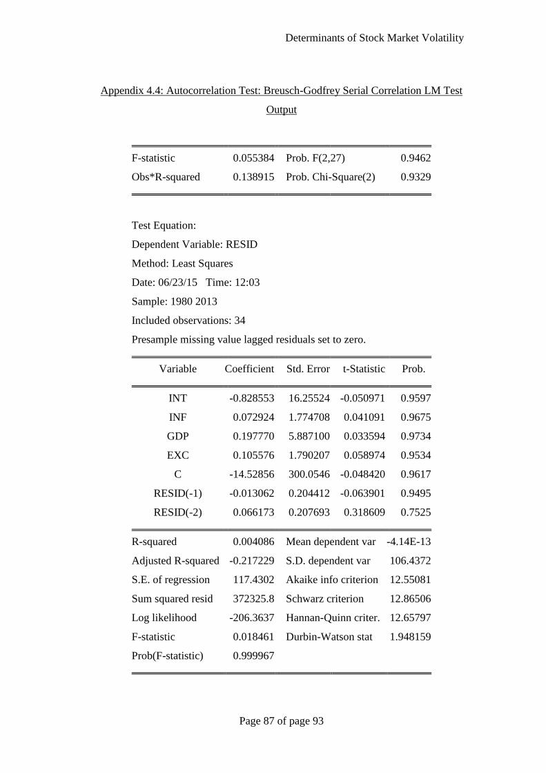
Determinants of Stock Market Volatility
Page 87 of page 93
Appendix 4.4: Autocorrelation Test: Breusch-Godfrey Serial Correlation LM Test
Output
F-statistic 0.055384 Prob. F(2,27) 0.9462
Obs*R-squared 0.138915 Prob. Chi-Square(2) 0.9329
Test Equation:
Dependent Variable: RESID
Method: Least Squares
Date: 06/23/15 Time: 12:03
Sample: 1980 2013
Included observations: 34
Presample missing value lagged residuals set to zero.
Variable Coefficient Std. Error t-Statistic Prob.
INT -0.828553 16.25524 -0.050971 0.9597
INF 0.072924 1.774708 0.041091 0.9675
GDP 0.197770 5.887100 0.033594 0.9734
EXC 0.105576 1.790207 0.058974 0.9534
C -14.52856 300.0546 -0.048420 0.9617
RESID(-1) -0.013062 0.204412 -0.063901 0.9495
RESID(-2) 0.066173 0.207693 0.318609 0.7525
R-squared 0.004086 Mean dependent var -4.14E-13
Adjusted R-squared -0.217229 S.D. dependent var 106.4372
S.E. of regression 117.4302 Akaike info criterion 12.55081
Sum squared resid 372325.8 Schwarz criterion 12.86506
Log likelihood -206.3637 Hannan-Quinn criter. 12.65797
F-statistic 0.018461 Durbin-Watson stat 1.948159
Prob(F-statistic) 0.999967

Determinants of Stock Market Volatility
Page 88 of page 93
Appendix 4.5: Multicollinearity Test: Auxiliary Model 1
Dependent Variable: INT
Method: Least Squares
Date: 06/23/15 Time: 12:04
Sample: 1980 2013
Included observations: 34
Variable Coefficient Std. Error t-Statistic Prob.
INF -0.027019 0.020263 -1.333410 0.1924
GDP 0.011150 0.069677 0.160018 0.8739
EXC 0.018754 0.020168 0.929895 0.3598
C 4.051066 3.429223 1.181336 0.2467
R-squared 0.303300 Mean dependent var 4.224706
Adjusted R-squared 0.233630 S.D. dependent var 1.596740
S.E. of regression 1.397827 Akaike info criterion 3.617845
Sum squared resid 58.61758 Schwarz criterion 3.797417
Log likelihood -57.50337 Hannan-Quinn criter. 3.679084
F-statistic 4.353381 Durbin-Watson stat 0.678919
Prob(F-statistic) 0.011646

Determinants of Stock Market Volatility
Page 89 of page 93
Appendix 4.6: Multicollinearity Test: Auxiliary Model 2
Dependent Variable: INF
Method: Least Squares
Date: 06/23/15 Time: 12:05
Sample: 1980 2013
Included observations: 34
Variable Coefficient Std. Error t-Statistic Prob.
INT -2.070777 1.552993 -1.333410 0.1924
GDP 0.429474 0.605194 0.709647 0.4834
EXC -0.691146 0.127082 -5.438580 0.0000
C 155.6055 11.66609 13.33828 0.0000
R-squared 0.643703 Mean dependent var 72.88223
Adjusted R-squared 0.608074 S.D. dependent var 19.54717
S.E. of regression 12.23731 Akaike info criterion 7.956987
Sum squared resid 4492.555 Schwarz criterion 8.136559
Log likelihood -131.2688 Hannan-Quinn criter. 8.018227
F-statistic 18.06650 Durbin-Watson stat 0.195002
Prob(F-statistic) 0.000001

Determinants of Stock Market Volatility
Page 90 of page 93
Appendix 4.7: Multicollinearity Test: Auxiliary Model 3
Dependent Variable: GDP
Method: Least Squares
Date: 06/23/15 Time: 12:05
Sample: 1980 2013
Included observations: 34
Variable Coefficient Std. Error t-Statistic Prob.
INF 0.038441 0.054169 0.709647 0.4834
INT 0.076487 0.477988 0.160018 0.8739
EXC 0.093671 0.050777 1.844765 0.0750
C -7.552773 9.084170 -0.831421 0.4123
R-squared 0.151692 Mean dependent var 5.943824
Adjusted R-squared 0.066861 S.D. dependent var 3.790033
S.E. of regression 3.661139 Akaike info criterion 5.543556
Sum squared resid 402.1181 Schwarz criterion 5.723128
Log likelihood -90.24046 Hannan-Quinn criter. 5.604796
F-statistic 1.788169 Durbin-Watson stat 1.632660
Prob(F-statistic) 0.170677

Determinants of Stock Market Volatility
Page 91 of page 93
Appendix 4.8: Multicollinearity Test: Auxiliary Model 4
Dependent Variable: EXC
Method: Least Squares
Date: 06/23/15 Time: 12:06
Sample: 1980 2013
Included observations: 34
Variable Coefficient Std. Error t-Statistic Prob.
INF -0.718314 0.132077 -5.438580 0.0000
INT 1.493852 1.606474 0.929895 0.3598
GDP 1.087650 0.589587 1.844765 0.0750
C 150.3020 15.07488 9.970359 0.0000
R-squared 0.667624 Mean dependent var 110.7256
Adjusted R-squared 0.634386 S.D. dependent var 20.63226
S.E. of regression 12.47551 Akaike info criterion 7.995542
Sum squared resid 4669.147 Schwarz criterion 8.175114
Log likelihood -131.9242 Hannan-Quinn criter. 8.056781
F-statistic 20.08638 Durbin-Watson stat 0.232396
Prob(F-statistic) 0.000000

Determinants of Stock Market Volatility
Page 92 of page 93
Appendix 4.9: OLS FinalOutput
Dependent Variable: KLCI
Method: Least Squares
Date: 06/23/15 Time: 12:07
Sample: 1980 2013
Included observations: 34
Variable Coefficient Std. Error t-Statistic Prob.
INT 23.74633 14.82988 1.601249 0.1202
INF 28.97065 1.693967 17.10225 0.0000
GDP 20.93754 5.662064 3.697863 0.0009
EXC 10.70877 1.661624 6.444760 0.0000
C -2727.480 284.9492 -9.571811 0.0000
R-squared 0.934313 Mean dependent var 794.4709
Adjusted R-squared 0.925253 S.D. dependent var 415.2933
S.E. of regression 113.5407 Akaike info criterion 12.43725
Sum squared resid 373853.3 Schwarz criterion 12.66172
Log likelihood -206.4333 Hannan-Quinn criter. 12.51380
F-statistic 103.1224 Durbin-Watson stat 1.997425
Prob(F-statistic) 0.000000

Determinants of Stock Market Volatility
Page 93 of page 93
Appendix 5.0: Correlation Output
KLCI INT INF GDP EXC
KLCI 1.000000 -0.318710 0.855870 0.106762 -0.421134
INT -0.318710 1.000000 -0.526848 0.188786 0.511867
INF 0.855870 -0.526848 1.000000 -0.219124 -0.785225
GDP 0.106762 0.188786 -0.219124 1.000000 0.370743
EXC -0.421134 0.511867 -0.785225 0.370743 1.000000