Determinants of Household Saving in Australia*

Mark N. Harris, Joanne Loundes and Elizabeth WebsterMelbourne Institute of Applied Economic and Social Research

The University of Melbourne

Melbourne Institute Working Paper No. 22/99

ISSN 1328-4991

ISBN 0 7340 1476 7

October 1999

* The authors are grateful for helpful comments from John Creedy and seminarparticipants at the Melbourne Institute and the 28th Annual Conference of Economists atLa Trobe University.

Melbourne Institute of Applied Economic and Social ResearchThe University of Melbourne

Parkville, Victoria 3052 AustraliaTelephone (03) 9344 5330

Fax (03) 9344 5630Email melb.inst@iaesr.unimelb.edu.au

WWW Address http://www.ecom.unimelb.edu.au/iaesrwww/home.html

Abstract

This paper uses a unique survey of consumers (incorporating theMelbourne In-

stitute Household Savings Survey and the Westpac-Melbourne Institute Survey of

Consumer Sentiment) to examine the determinants of Australian household sav-

ing. Unit records from 17,700 Australian households are available, which enables

the incorporation of a range of household characteristics that may be important

factors for saving behaviour, but which are not typically available to researchers

undertaking macroeconomic analyses. An ordered probit estimation method is

used, and the results support the view that current incomes are perhaps the most

important determinant of saving. However, it can also be seen that demographics

and householders level of economic optimism play a key role.

2

1. Introduction

This paper uses a unique survey of consumers (incorporating the Melbourne In-

stitute Household Savings Survey and the Westpac-Melbourne Institute Survey of

Consumer Sentiment) to examine the determinants of Australian household sav-

ing. Unit records from 17,700 Australian households are available, which enables

the incorporation of a range of household characteristics that may be important

factors for saving behaviour, but which are not typically available to researchers

undertaking macroeconomic analyses. For example, the distribution of savings

across households is important to governments who uphold an economic safety

net function, such that an even distribution of assets across families should lessen

the burden on welfare payments that buffer against unforeseen contingences. Ad-

ditionally, as an economy’s population ages, it may lower the dependence on gov-

ernment aged pensions. Changing household demographics can also play a role

in shaping national saving. Perhaps most importantly however is that an under-

standing of household saving behaviour can assist policy makers in assessing the

likely impact on saving of changes in economic circumstances facing households

[both anticipated (the introduction of the GST or retirement) and unanticipated

(an unexpected depreciation of the exchange which adversely influences prices)].

High savings ratios do not of course necessarily imply high levels of saving, for

the latter also depends on the level of national income.1 Nor are higher saving

ratios of unlimited benefit, for they come at the cost of lower current consumption

ratios. If, for example, households tend to save more if they are pessimistic about

their economic future, then a negative external shock to the economy may be

compounded by the associated contraction in consumption. It is a question of

balance.

Most theories of saving are developed in terms of individuals’ motives, but

(in Australia at least) the majority of empirical work has utilised aggregate times

series data. In some cases this is because of a paucity of reliable household in-

formation sets on Australian household saving ((Defris 1977); (Lattimore 1994);

(Lester 1996)), although in others it has been suggested that private rather than

1The ‘paradox of thrift’ dilemma can be managed however by compensating stimulus toconsumption or other sources of final demand.

1

household saving per se is a more appropriate focus for macro policy purposes

(Edey and Britten-Jones 1990). These studies find that household disposable in-

come provides most of the explanatory power; the inclusion of variables such as

interest rates and wealth is found to have little or no effect.2 Aggregate analy-

sis also suggests that consumption smoothing behaviour is only important over

relatively short periods (Edey and Britten-Jones 1990).

More recently, there has been a shift in the empirical literature from aggre-

gate time series studies toward individual household analysis, partly because of

the observation that very little has been learned about individual saving behaviour

from time series work. Aggregate analysis tends to ignore demographics (primar-

ily because they change only gradually in the aggregate), but it is exactly such

demographics that can be potentially important sources of variation in saving at

the micro level (Browning and Luscardi 1996). This was one of the original moti-

vations behind establishing an Australian household saving survey, as well as the

view that survey data are more likely to quickly pick up information on changes

in household behaviour in response to changes in economic or political conditions

(McDonnell and Williams 1994).

Section 2 further describes the data set to be utilised and presents cross tabu-

lated results on households stated motives for saving. An outline of the models to

be used is given in Section 3. These models incorporate a range of variables that

were chosen to reflect some of the key determinants of savings as outlined in such

hypotheses as the life-cycle hypothesis, the absolute income hypothesis, the rela-

tive income hypothesis, and precautionary motives for saving. The results from

the ordered probit estimation are then discussed in Section 4. One of the difficul-

ties with interpreting ordered probit estimates is that the impact of a change in an

explanatory variable on the intermediate classification of the dependent variable

cannot be determined a priori. In order to overcome this problem, some extra

analysis is presented that investigates this intermediate impact. Section 5 finishes

with a short conclusion.

2One of the major criticisms of this work is that imputing savings from national accountsestimates includes a high degree of measurement error, a problem that is also encountered inthe cross sectional Household Expenditure Survey.

2

2. Data set

The Melbourne Institute Household Saving Survey is conducted by telephone,

and the questions are put to a random sample of 1200 households each quarter.3

The survey records several qualitative measures on the extensiveness of household

saving, reasons for saving and asset allocation. In addition it includes information

on the age of the respondent, household incomes, respondents gender and the

presence of children. The data used in the estimation were derived from the

pooled results of the quarterly surveys over the period August 1994 to February

1999, giving a total sample size of 17,700 people 18 years and over across Australia.

To complement the formal estimation of what influences household saving,

self enumerated reasons for saving from the survey are given in Table 2.1. Such

an exercise is important, because characterising why people save can have impli-

cations for the amount they save. The top three motives are for retirement (a

life-cycle motive), holidays, and a rainy day (the precautionary motive). There

is a relatively large break between the top three and the next four reasons for

saving, which are to invest in the family home, pay off debt, education and to buy

durables. The bequest motive is relatively unimportant.

Comparing across income groups, there is a substantially higher proportion

of low-income individuals (under $20,000 per annum) who have no savings. Of

those who do save, the most important reason is for precautionary factors (rainy

day), followed by the retirement and holiday motives. Compared to the other

income categories, saving for educational purposes rates very poorly. As income

increases, saving for retirement becomes the most important reason for saving,

although for households with an annual income of between $21,000 and $40,000,

precautionary saving still ranks quite highly.

Table 2.2 presents data on motives for saving by age group, and whether or

not there are children in the household. For the youngest age group (18 to 24)

holidaying and buying durables are the most important reasons for saving. Middle

aged respondents (25 to 44) also rate holidays as a high priority, followed closely

by investing in the family home and saving for retirement. Saving for education

3The sample was stratified by sex and location and age was randomised. The NorthernTerritory was not included.

3

Table 2.1: Main reasons for saving by income category (per cent of householdsstating each reason, 1994 to 1999) a

Total Under $20k $20k to $40k $40k to $60k $60k and over

Sample size 17690 4148 5373 3911 4258Retirement 34 22 33 40 44Holiday 31 20 27 36 40Rainy day (e.g. unemployment) 29 29 30 29 26Buy, improve, upgrade home 22 10 21 27 30Pay off debt 21 13 21 25 24Education 20 9 21 25 22Buy durables (e.g. car) 17 10 17 19 21Bequest 9 7 9 10 8Other 8 8 7 7 8Don’t know 1 1 1 0 0No saving 12 24 11 6 5

Source: Melbourne Institute Household Savings Survey, unpublished data

Notes: aMultiple reasons were permitted.

is also considered relatively important for this age group. Saving for retirement

is the single most important reason for saving for respondents over the age of 45.

This age group also appears more risk averse than other age groups; precautionary

saving ranks second, whereas it only ranks 6th for the 18 to 24 year olds and 5th

for the 25 to 44 year olds. A higher proportion of this category has no savings

at all, which is not surprising given that this group contains a number of retired

individuals. Compared with the youngest respondents, buying durables does not

rate very highly for people over the age of 25.

The primary difference in saving motives between households with and without

children is in saving for educational purposes. Two out of every five respondents

that had children present in the household indicated they saved for this purpose,

compared to only one in fourteen for households without children. Paying off

debt also rated as a high priority for households with children compared to those

without children.

In sum, householders stated reasons provides further depth on the motives for

saving, and give a useful counterpoint for the indirect evidence from the regression

analysis. These results indicate that income is going to be an important factor

in determining saving, but also add support to the life cycle and precautionary

hypotheses.

4

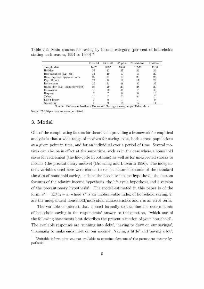
Table 2.2: Main reasons for saving by income category (per cent of householdsstating each reason, 1994 to 1999) a

18 to 24 25 to 44 45 plus No children Children

Sample size 1467 8337 7886 10552 7138Holiday 37 32 27 32 29Buy durables (e.g. car) 34 19 10 15 20Buy, improve, upgrade home 29 31 10 20 25Pay off debt 27 28 12 17 28Retirement 26 31 41 35 33Rainy day (e.g. unemployment) 25 29 29 28 29Education 18 29 9 7 40Bequest 6 7 8 6 13Other 10 7 7 8 7Don’t know 0 0 1 1 0No saving 4 9 16 12 11

Source: Melbourne Institute Household Savings Survey, unpublished data

Notes: aMultiple reasons were permitted.

3. Model

One of the complicating factors for theorists in providing a framework for empirical

analysis is that a wide range of motives for saving exist, both across populations

at a given point in time, and for an individual over a period of time. Several mo-

tives can also be in effect at the same time, such as in the case where a household

saves for retirement (the life-cycle hypothesis) as well as for unexpected shocks to

income (the precautionary motive) (Browning and Luscardi 1996). The indepen-

dent variables used here were chosen to reflect features of some of the standard

theories of household saving, such as the absolute income hypothesis, the custom

features of the relative income hypothesis, the life cycle hypothesis and a version

of the precautionary hypothesis4. The model estimated in this paper is of the

form, s∗ = Σβixi + ε, where s∗ is an unobservable index of household saving, xi

are the independent household/individual characteristics and ε is an error term.

The variable of interest that is used formally to examine the determinants

of household saving is the respondents’ answer to the question, “which one of

the following statements best describes the present situation of your household”.

The available responses are ‘running into debt’, ‘having to draw on our savings’,

‘managing to make ends meet on our income’, ‘saving a little’ and ‘saving a lot’.

4Suitable information was not available to examine elements of the permanent income hy-pothesis.

5

The answers are used as a proxy for a saving ratio, as it is assumed that re-

spondents answers are relative to their income. As these responses are (ordered)

categorical (i.e. the choices range from 0 to 4), the estimation method used here

is an ordered probit. For identification purposes, all boundary parameters can

be estimated without a constant, or, if a constant is included, the first boundary

parameter must be restricted to zero (the latter method is utilised here). Addi-

tionally, the error term is specified as having a mean of zero and a variance of

one.

The model assumes that the observed saving response, s, is related to an

underlying latent variable–that of the actual monetary amount describing the

household’s financial position with regard to savings and debt, s∗. Saving is de-

termined not only by s∗, but also by its relationship to the boundary parameters,

µj which jointly determine the observed outcome. That is, given the five alterna-

tives outlined above, the following is observed

s =

0 if s∗ ≤ 0,1 if 0 < s∗ ≤ µ1,2 if µ1 < s

∗ ≤ µ2,3 if µ2 < s

∗ ≤ µ3,4 if µ3 ≤ s∗.

Dependent on the hypothesis of interest, s∗ is a function of certain personal

(and macroeconomic) variables xi, with unknown weights β. Assuming a linear

relationship and a random sample of N individuals i = 1, . . . ,N , the following is

obtained

s∗i = x"iβ + ui. (3.1)

If the ui of equation (3.1) are independently standard normally distributed,

the probability that individual i “chooses” alternative j ( j = 0, . . . , J − 1)5 isProb (si = 0) = Φ

%−x"iβ

&,

Prob (si = 1) = Φ%µ1 − x"iβ

&−Φ

%−x"iβ

&,

Prob (si = 2) = Φ%µ2 − x"iβ

&−Φ

%µ1 − x"iβ

&,

Prob (si = 3) = Φ%µ3 − x"iβ

&−Φ

%µ2 − x"iβ

&, and

Prob (si = 4) = 1− Φ%µ3 − x"iβ

&,

5J is the total number of alternatives, here J = 5.

6

with the requirement that 0 < µ1 < . . . < µJ−2 and where Φ is the standard nor-

mal cumulative distribution function. Maximum likelihood parameter estimates

are obtained by maximising the likelihood

log L =N'

i=1

J'j=0

zijlog (Pij) (3.2)

with respect to β and µ, where zij is an indicator variable equal to unity if indi-

vidual i chooses alternative j and zero otherwise.

The variables used in the estimation (along with their mean values) are con-

tained in Table 3.1, and a full explanation follows. Most are entered as zero-one

indicator (dummy) variables. Variables that are ordered qualitative in nature are

also entered as dummies to avoid forcing quantitative effects onto a qualitative

variable.6

The household saving ratio is measured on the 5 point scale discussed above.7

This variable could be criticised on the grounds that it is a self-reported qualita-

tive measure, and that there is no way of telling what types of saving respondents

have included in their views on how much they are saving (such as superannua-

tion or mortgage repayments). However it can still be considered a useful proxy

given that it avoids the measurement bias found in any of the available direct

measures of income, consumption and saving. Household incomes were grouped

into $10,000 per annum sets, starting from $21,000 or below, up to $100,000 and

over. Respondent’s age was grouped as 18 to 24, 25 to 34, 35 to 44, 45 to 49, 50 to

54, 55 to 64 and 65 years and over. The rate of interest was the average quarterly

rate offered by major trading banks on fixed deposits. Children were measured

by the number of people living in the household under the age of 18. There were

two variables to indicate comparative wealth. The first was a dummy variable to

indicate whether the respondent wholly or partially owned a house. The second

was a dummy variable to indicate whether their main asset holdings were in the

form of shares, bonds, debentures, managed trusts, holiday homes or investment

properties.

6The main drawback of this is that sources of variation in the data are potentially being lost.7Theoretically, savings should also include debt repayments, but it has not been possible to

include these factors in the dependent variable given the ordinal nature of the survey response.

7

Table 3.1: Sample means

Means Standard DeviationMale 51 50.0

Interest rate 6 1.6Optimism 1 0.2

Below median income 41 49.2Above median income 38 48.5

Income 44538 29001.018-24 years old 8 27.625-34 years old 21 40.935-44 years old 26 43.845-49 years old 11 31.050-54 years old 9 28.355-64 years old 11 31.6Home owner 80 40.3

Wealth 36 47.9Number of children 1 1.2Children present 40 49.1Urban dweller 58 49.4

New South Wales 27 44.4Victoria 24 42.9

Queensland 17 37.3South Australia 13 33.6

Western Australia 13 33.3

8

According to the relative income hypothesis, people spend according to what

is normal for their reference group and past consumption levels (i.e. they save if

income is high relative to their peers or income has risen and vice versa). In order

to calculate relative income, the peer group for respondents was proxied using the

median income level for the respondents occupation, as measured by the survey.

A variable was then constructed to denote whether household income was above,

below or at this median occupational income level. Occupations were classified at

the major Australian Standard Classification of Occupations (1st edition) level.

As the data are cross sectional, it was not possible to construct a variable for that

enabled the habit aspect of Duesenberry’s hypothesis to be examined.

There is evidence to suggest that subjective factors are an important deter-

minant of household savings (Carroll and Samwick 1995, Browning and Luscardi

1996), and the primary problem has been finding an observable and exogenous

variable to signify the householders’ degree of uncertainty or economic pessimism.

Typically, these studies use indirect measures of the subjective motives for savings

such as income variance and insurance coverage. However, the data set used here

incorporates a direct question on consumer sentiment which allows household sav-

ing to be cross classified against their degree of economic optimism/pessimism.

This precautionary variable was calculated as an average of responses to questions

about the future of family finances, the Australian economy over the coming year

and over the next 5 years, and expectations about unemployment over the next

year. Responses were rated on a 5 point scale. These responses were weighted

evenly around the neutral response of 3 and summed. Unfortunately, this measure

of expectations shows a significant positive correlation with the householder’s cur-

rent circumstances and is thus likely to be endogenous to the dependent variable.

To obtain a variable that was free from these effects, the constructed expectations

variable was divided by two responses about the householder’s current economic

circumstances. These referred to householders financial situation over the last

year and their views on current buying conditions. The resulting variable ‘opti-

mism’ should give a measure of householders optimism regarding future economic

prosperity for themselves and the Australian economy, given their current circum-

stances.

9

4. Results

Table 4.1 gives the results for the model that conditions on relative income, and ta-

ble 4.2 presents results conditioning on the absolute income levels of respondents.

Care should be taken when interpreting coefficients on ordered probit estimates,

as they do not represent marginal values. A positive and significant coefficient

indicates that a particular characteristic implies a greater probability of being

in a higher saving category, and vice versa for a negative and significant coeffi-

cient. Additionally, the absolute magnitude of the coefficients cannot be given

any meaning, because of the identifying restriction that the variance on ε equals

one.

The positive and significant coefficient on the male variable may possibly re-

flect the accepted view that men have higher saving in the form of superannuation

than women. A cross classification of gender by size of household indicates that

the male is more likely to be the respondent for two and four-person households,

which could suggest that the male respondent knows more about the financial

position of the household (i.e. the size of superannuation contributions) than the

female respondent.

Changes in the real rate of interest are hypothesised to have an ambiguous

effect on the level of saving, because there is both an income and substitution

effect.8 Empirical estimation usually finds at most only weak evidence of a small

positive impact on aggregate saving ((Callen and Thimann 1997); (Edey and

Britten-Jones 1990)). The results in Table 4.1 indicate that the interest rate has

no significant effect on Australian household saving ratios. It is more likely that

a change in interest rates will change the mix of saving, but may not necessarily

change the level.

Following Keynes’s early emphasis on the influence of expectations on savings

decisions, there has been a recent spate of models in the USA which have sought

to test the sensitivity of households savings ratios toward subjective factors, both

cyclical and irregular ((Browning and Luscardi 1996); (Carroll and Samwick 1998);

(Juster and Taylor 1975)). Specifically, these precautionary theories maintain that

the more uncertain or pessimistic are consumers about the future, the higher are

8See Keynes ([1936], 1973: Ch 8).

10

Table 4.1: Nested Model - Income Variable Omitted

Coefficient Standard Error

Constant 1.911 0.080∗∗

×1 (male) 0.150 0.016∗∗

Interest rate -0.009 0.005Optimism -0.644 0.049∗∗

×1 (Rel. low income) 0.001 0.022×1 (Rel. high income) 0.394 0.022∗∗

×1 (18-24 years old) 0.406 0.038∗∗

×1 (25-34 years old) 0.401 0.033∗∗

×1 (35-44 years old) 0.222 0.033∗∗

×1 (45-49 years old) 0.108 0.037∗∗

×1 (50-54 years old) 0.095 0.037∗∗

×1 (55-64 years old) -0.047 0.035Home owner 0.101 0.021∗∗

Wealth 0.365 0.018∗∗

# of children -0.040 0.012∗∗

×1 (children) -0.185 0.030∗∗

×1 (urban area) 0.064 0.017∗∗

×1 (New South Wales) 0.013 0.037×1 (Victoria) -0.009 0.037×1 (Queensland) -0.036 0.039×1 (South Australia) -0.049 0.040×1 (Western Australia) -0.006 0.040µ1 0.565 0.014∗∗

µ2 1.877 0.018∗∗

µ3 3.326 0.022∗∗

Log Likelihood -21,419.85Notes: ∗∗ and ∗ significant at 5% 2-sided and 1-sided levels, respectively.

11

their savings in order to meet both unforeseen and anticipated contingencies. As

such, it is expected that the sign on the coefficient of the precautionary variable

‘optimism’ will be negative. The results in Table 4.1 show that this coefficient is

negative and significant, indicating that if individuals are pessimistic about their

future financial situation and economic conditions, they are likely to be saving

more.

The relative income hypothesis (Duesenberry 1949) suggests that tastes, the

parameters of the utility function, are endogenous to past and present saving de-

cisions. In particular, tastes are shaped by social comparisons (custom) and past

consumption decisions (habit). As a result, the saving ratio is posited to depend

on the household’s income relative to their peers and current income relative to

past income but not absolute income levels. Due to the cross sectional nature

of the data, it is not possible to examine current income relative to past income.

The results on the distribution of income are given in Table 4.1 and show that the

coefficient on ‘relative high income’ significant and, as expected, positive, indicat-

ing that this group is more likely to be represented in the ‘saving a lot’ category.

This is in line with other microeconomic empirical work on the determinants of

household savings, which find that relative incomes are the most important deter-

minant of the saving ratio (Browning and Luscardi 1996). At the other end of the

income scale, the coefficient on ‘relative low income’ is not significantly different

from the omitted category, relative median income. Duesenberry (1949) suggested

that families with low relative occupational incomes would have to balance their

budgets on average, with dissaving only being a temporary phenomenon.

Modigliani and Brumberg’s (1953) life cycle hypothesis contends that saving

and dissaving are undertaken to smooth consumption and utility as yearly income

varies over the stages of the life-cycle. Over the course of a life time, young agents

borrow to consume in advance of future income, repay their debt and save through

the middle years (at which point they have a rising saving ratio) and finally, draw

down their savings after retirement.9 The coefficients on the age parameters

9Identifying life cycle profiles however is complicated by ‘cohort effects’; for example, a groupof 45 year olds in 1979 may have different savings patterns to a group of 45 year olds in 1999.See, for example, (Attanasio 1998). Additionally, different members of a household may havedifferent propensities to save. See, for example, (Browning 1994).

12

indicate that saving is positive relative to the omitted category (individuals aged

65 years and over) with the exception of respondents aged between 55 and 64.

Assets based theories of savings ((Houthakker and Taylor 1970); (Tobin 1951))

are an adaptation of the absolute income hypothesis. It includes a stock adjust-

ment process so that saving is positive when the level of wealth falls below the op-

timal level and negative otherwise, implying that households have a target wealth

to income ratio. Although it is not possible to examine optimal levels of wealth

for each household, it is possible to look at whether holding wealth or owning a

home influences saving ratios. From these estimates it appears that home owners

are likely to be saving more. Although the saving question does not explicitly

include mortgage repayments as savings, there is a possibility that respondents

view such repayments as saving, and may therefore indicate that they are ‘saving

a lot’. Respondents indicating they had any form of wealth also appeared more

likely to be in the higher saving categories, and could be attributed to the flows

of income from this stock of wealth going back in to some form of saving.

Given that the saving and consumption needs of households with children are

different to those without ((Kooreman and Wunderink 1997); (Pashardes 1991)),

it is expected that the presence of children will influence Australian household

saving ratios. Empirical estimates for the USA indicate that the saving of couples

is negatively correlated with the number of children and the age of the youngest

child (Wang 1994). The reasoning (apart from the obvious increased implied

expenditure) is that the addition of children to the household increases the price

of time. This makes leisure more expensive, thereby causing couples to increase

their labour force participation, consume more time saving goods and services, and

save less. Browning and Luscardi (1996, p 1815) also corroborate these results,

reporting that saving ratios are higher for couples with no children, lower for

households with children, and the least for lone parents. As can be seen from

Table 4.1, the coefficient is negative and significant for both the number of children

and whether or not there are children in the household, which is in line with the

evidence mentioned above. This indicates that the presence of children has a

detrimental effect on the probability of having a higher saving ratio, and the more

children a household has, the more difficulty a household has in saving anything.

13

Over time, this may have implications for aggregate saving if – as is the case

with a number of industrialised countries – fertility rates decline to the extent

where there are significantly fewer households with larger numbers of children.

The boundary parameters (µ1 to µ3) are strongly significant, indicating ev-

idence of ordering in the data. In order to capture any possible heterogeneity

relating to location, State dummies were also included, but proved to be insignif-

icant. However, the coefficient on the variable indicating whether the respondent

resided in an urban area was significant, although this may reflect the observation

that urban residents have a higher disposable income.10

Table 4.2 presents results conditioning on the absolute income levels of respon-

dents. The archetypal ‘Keynesian’ absolute income hypothesis depicts saving as

a positive linear function of income, wealth and interest rates, with a positive in-

tercept. It is generally recognised that relatively high income earners account for

a large share of aggregate savings ((Carroll 1998); (Callen and Thimann 1997))

and that a substantial proportion of households never accumulate large stocks of

financial wealth ((Poterba and Samwick 1997); (Browning and Luscardi 1996)).

Evidence from the USA suggests that households with higher levels of lifetime in-

come also tend to have higher lifetime savings ratios (Carroll 1998), and estimates

for Australia indicate that the wealthiest 10 per cent of the population hold more

than half of Australian wealth (Dilnot 1990). In their review of the literature,

Browning and Luscardi (1996) suggest that saving is usually negative for the first

and second income quintile and highest in the top quintile. In line with evidence

from elsewhere, the coefficient on the absolute income variable is (as expected)

positive and significant, suggesting that saving ratios rise with the level of income.

It has been suggested that lower saving may in fact be an optimal choice for low-

income households if welfare payments are means-tested (Hubbard, Skinner, and

Zeldes 1995). Other evidence from Australia indicates that a relatively large share

of individuals who are not working have no savings at all (Loundes 1999). This

is consistent with evidence from other OECD countries, where unemployment is

so detrimental to saving that the ‘lower income’ effect outweighs the ‘need for

precautionary saving’ effect (Callen and Thimann 1997).

10Remembering that this version of the model does not condition on levels of income.

14

Table 4.2: Nested Model - RIH Variables Omitted

Coefficient Standard Error

Constant 1.822 0.078∗∗

×1 (male) 0.070 0.017∗∗

Interest rate -0.003 0.005Income 0.142 0.003∗∗

Optimism -0.576 0.049∗∗

×1 (18-24 years old) 0.220 0.038∗∗

×1 (25-34 years old) 0.164 0.033∗∗

×1 (35-44 years old) -0.026 0.034×1 (45-49 years old) -0.140 0.037∗∗

×1 (50-54 years old) -0.095 0.038∗∗

×1 (55-64 years old) -0.131 0.036∗∗

Home owner 0.030 0.021Wealth 0.252 0.018∗∗

# of children -0.029 0.012∗∗

×1 (children) -0.172 0.030∗∗

×1 (urban area) 0.004 0.017×1 (New South Wales) -0.044 0.037×1 (Victoria) -0.020 0.037×1 (Queensland) -0.045 0.039×1 (South Australia) -0.034 0.040×1 (Western Australia) -0.031 0.040µ1 0.575 0.014∗∗

µ2 1.926 0.018∗∗

µ3 3.438 0.023∗∗

Log Likelihood -20,905.55Notes: ∗∗ and ∗ significant at 5% 2-sided and 1-sided levels, respectively.

15

‘Residual’ hypotheses of saving (Marglin 1975) maintain that apart from the

decision to save for a house, most household saving is the residual of income after

consumption and does not emanate from a deliberate decision to save.11 Such an

argument implies that, a priori, low-income households will save less than high

income, simply because they have a lower disposable income (although it should

be noted that the relationship between saving and income is two-way). This

proposition would be difficult to test, because although this may be the case,

there are very few households who are likely to explicitly state, even when asked

why they save, that this is the reason they currently have any savings.

Conditioning on absolute incomes does produce some differences with the re-

sults presented in Table 4.1. The major difference concerns the estimated coeffi-

cients on the age variables. In this model, the coefficient on individuals over the

age of 45 are negative and significant. What this implies is that absolute incomes

account for the bulk of saving once an individual is over the age of 35. Once

the absolute level of income is conditioned on for these age groups, it is found

that older individuals are actually more likely to have a lower saving rate than

the youngest. The other changes in the estimates are that home ownership and

residing in an urban area are no longer significant explanators of saving ratios,

which suggests that income levels account for the bulk of the explanatory power

of these two variables in the previous estimation.

4.1. Effects of Selected Variables on Saving Patterns

In an ordered probit model, the marginal effects of explanatory variables on the

choice probabilities are not the estimated coefficients. Moreover, although a pos-

itive coefficient unambiguously shifts probability mass out of the ‘running into

debt’ option and into ‘saving a lot’, it is unclear what happens to probabilities

in the other three options without undertaking further analysis. Essentially the

technique utilised to examine these effects involves estimating the choice proba-

bilities for two given sets of personal characteristics, where the two sets differ by

virtue of the variable(s) under consideration. The difference in these two sets of

11According to Keynes ([1936], 1973: 97) ‘satisfaction of immediate primary needs of a manand his family is usually a stronger motive than the motives towards accumulation’.

16

probabilities can be interpreted as the marginal effect on the choice probabilities

of this (these) variable(s). The variable of interest is given a range of “likely” val-

ues (zero/one for dummy variables), whilst the remaining explanatory variables

are evaluated at their sample means.12 Such an exercise was undertaken and the

results illustrated in Figures 1 to 8 below.

Figure 4.1: Effect on the saving ratio of increasing the interest rate from 1 to 10per cent.

0.0

0.1

0.2

0.3

0.4

0.5

running into debt drawing on savings no net saving saving a little saving a lot

saving pattern

1%

10%

pro

ba

bili

ty

In line with the results presented earlier, Figure 4.1 indicates that a relatively

large change in the interest rate (from 1 to 10 per cent) has virtually no effect

on saving ratios. Figure 4.2 shows that home ownership gives similar results.

However, more interesting estimates are obtained when the other variables are

examined.

A change in optimism also has an impact on the intermediate saving choices.

Figure 4.3 illustrates that nearly 70 per cent of ‘optimistic’ respondents are rep-

resented in the bottom three categories, compared just over 40 per cent of the

least optimistic. Based on these estimates, a negative shock to the economy that

12In terms of the parameters under analysis here, the likely values are: 1% and 10% for theinterest rate; 0.5 and 1.5 for the degree of optimism; below and above median income; 7 agegroups ranging from 18 to 24 up to 65 plus; wealth and no wealth; 0, 1 and 5 children; householdincome up to $20k, between $51 and $60k and over $100k; and whether the individual ownstheir own home or not.

17

Figure 4.2: Effect on the saving ratio of home ownership.

0.0

0.1

0.2

0.3

0.4

0.5

running into debt drawing on savings no net saving saving a little saving a lot

saving pattern

own house

not house ownerp

rob

ab

ility

increases consumer pessimism will increase the number of people saving by a

considerable proportion.

Figure 4.3: Effect on the saving ratio of an increase in optimism.*

0.0

0.1

0.2

0.3

0.4

0.5

running intodebt drawingon savings nonet saving savinga little savinga lot

savingpattern

0.5 (morepessimistic)1.5 (moreoptimistic)

pro

bab

ility

*Theoptimismvariable is approximately~N(1, 0.17).

Figure 4.4 shows how being in different age groups affects the saving ratio.

These results belie the expected profile, that is, the youngest and oldest age groups

will be disproportionately represented in the bottom three saving categories, and

the middle age group will have a higher share of the top two categories. However,

conditioning on incomes removes this effect, resulting in the observation that

18

young individuals are saving more than their elders.

Figure 4.4: Effect on the saving ratio of different age groups.

0.0

0.1

0.2

0.3

0.4

0.5

running intodebt drawingonsavings nonet saving savinga little savinga lot

savingpattern

18 to24 35 to44 50 to54 65+

pro

bab

ility

Figure 4.5: Effect on the saving ratio of the number of children.

0.0

0.1

0.2

0.3

0.4

0.5

running into debt drawing on savings no net saving saving a little saving a lot

saving pattern

0

1

5

pro

ba

bili

ty

Figure 4.5 illustrates the impact on saving if there are children in the house-

hold. Having one child increases the chance if the household only managing to

‘make ends meet’ by about 5 per cent, as compared to the case where there are no

children present. Households with five children are not particularly worse off than

households with one child, as the chance of being in the bottom three categories

19

is only around 6 per cent higher. There is however a relatively large difference

in being represented in the ‘saving a little’ category depending on whether the

household has no children, one child or five children, with about a five per cent

difference between each of these groups.

Figure 4.6: Effect on the saving ratio of wealth.

0.0

0.1

0.2

0.3

0.4

0.5

running into debt drawing on savings no net saving saving a little saving a lot

saving pattern

wealth

no wealth

pro

ba

bili

ty

Figure 4.7: Effect on the saving ratio of different income levels.

0.0

0.1

0.2

0.3

0.4

0.5

0.6

running intodebt drawingonsavings nonet saving saving a little savinga lot

savingpattern

incomeupto$20k income$51- 60k

income$100k+

pro

bab

ility

The estimates on the wealth variable shows a considerable impact on the

probability of shifting between saving categories. The bulk of the movement is

20

in the ‘no net saving’ and ‘saving a little’ categories, with wealthier individuals

around 10 per cent more likely to be ‘saving a little’ than respondents with no

wealth, and about 8 per cent less likely to be ‘managing to make end meet’.

Absolute income levels have a large impact on saving rates, as is illustrated

in Figure 4.7. Less than one quarter of households earning over $100,000 are in

the ‘no net saving’ category or below, compared to 70 per cent of households who

earn up to $20,000. More than 1 in 5 high income households are ‘saving a lot’,

which is by far the largest share of any of the categories presented here.

Figure 4.8 shows the effect of having above or below the median level of income

(for the respondents occupation) on the probability of falling within a particular

saving bracket. Households with a low relative income for their occupation are

15 per cent more likely to be running into debt, drawing on their savings, or

just managing to make ends meet as compared to the relatively high in come

households.

Figure 4.8: Effect on the saving ratio of differences in relative occupational income.

0.0

0.1

0.2

0.3

0.4

0.5

running intodebt drawingonsavings nonet saving savinga little savinga lot

savingpattern

abovemedian incomebelowmedian income

pro

bab

ility

5. Conclusion

The analysis of Australian household saving data support the view that incomes

are perhaps the most important determinant of saving. However, it can also be

seen that demographics and householders level of economic optimism play a key

21

role. Several issues can be addressed using these results. The observation that

saving rates are positively influenced by household income levels (relative and

absolute) and wealth could suggest that a more even distribution of income across

the population may encourage greater saving. From a macroeconomic viewpoint,

these estimates also support the general consensus that the level of the interest rate

has little or no influence on household saving ratios. Additionally, they suggest

that precautionary factors are an important determinant of household saving,

implying that shocks to the economy that unduly influence consumer sentiment

may lead to a temporary change in saving levels. The ability to draw numerous

inferences from this analysis that is not readily available from the standard time

series aggregates suggests that there is some merit in examining household level

data.

22

References

Attanasio, O. P. (1998): “A Cohort Analysis of Saving Behaviour by U.S.Households,” Journal of Human Resources, 33(3), 575—609.

Browning, M. (1994): “The Saving Behaviour of a Two-Person Household,”Working Paper 9406, Department of Economics, McMaster University.

Browning, M., and A. Luscardi (1996): “Household Saving: Micro Theoriesand Micro Facts,” Journal of Economic Literature, XXXIV(4), 1797—1855.

Callen, T., and C. Thimann (1997): “Empirical Determinants of HouseholdSaving: Evidence from O.E.C.D. Countries,” Working Paper 181, InternationalMonetary Fund.

Carroll, C. D. (1998): “Why Do the Rich Save so Much?,” Working Paper338, Department of Economics, John Hopkins University.

Carroll, C. D., and A. A. Samwick (1998): “How Important is Precaution-ary Saving?,” Review of Economics and Statistics, 80(3), 410—19.

Defris, L. V. (1977): “Australian Consumer Expectations Evaluations, Uncer-tainty and the Saving Ratio,” Australian Economic Review, 1st Quarter, 36—42.

Dilnot, A. W. (1990): “The Distribution and Composition of Personal SectorWealth in Australia,” Australian Economic Review, 1st Quarter, 33—40.

Duesenberry, J. S. (1949): Income, Saving and the Theory of Consumer Be-havior. Harvard University Press, Cambridge.

Edey, M., and M. Britten-Jones (1990): “Saving and Investment in the1980s,” in The Australian Macro-Economy in the 1980s, ed. by S. Grenville,pp. 79—145, Sydney. Reserve Bank of Australia, Reserve Bank of Australia.

Houthakker, H., and L. Taylor (1970): Consumer Demand in the UnitedStates. Harvard University Press, Cambridge, 2nd edn.

Hubbard, R. G., J. Skinner, and S. P. Zeldes (1995): “PrecautionarySaving and Social Insurance,” Journal of Political Economy, 103(2), 360—99.

Juster, F. T., and L. D. Taylor (1975): “Personal Savings in the Post-war World: Implications for the Theory of Household Behaviour,” AmericanEconomic Review, 65(2), 203—209.

Kooreman, P., and S. Wunderink (1997): The Economics of HouseholdBehaviour. Macmillan Press, Houndmills, Basingstoke.

Lattimore, R. (1994): “Australian Consumption and Saving,” Oxford Reviewof Economic Policy, 10, 54—70.

Lester, L. H. (1996): “The Saving to Income Ratio,” Economic Analysis andPolicy, 26, 59—76.

23

Loundes, J. (1999): “Household Saving Behaviour in Australia,” Working Paper17/99, Melbourne Institute of Applied Economic and Social Research, Univer-sity of Melbourne, Melbourne.

Marglin, S. A. (1975): “What Do Bosses Do? Part II,” Review of RadicalPolitical Economics, 7(1), 20—37.

McDonnell, J., and R. Williams (1994): “Measuring Saving Intentions,”Australian Economic Review, 3rd Quarter, 64—74.

Pashardes, P. (1991): “Contemporaneous and Intertemporal Child Costs:Equivalent Expenditure vs Equivalent Income Scales,” Journal of Public Eco-nomics, 45(2), 191—213.

Poterba, J. M., and A. A. Samwick (1997): “Household Portfolio Allocationover the Life Cycle,” Working Paper 6185, N.B.E.R., Cambridge.

Tobin, J. (1951): Relative Income, Absolute Income and Savingpp. 135—56.Macmillan, New York.

Wang, Y. (1994): “Effects of the Price of Time on Household Saving: A Life-Cycle Consistent Model and Evidence from Micro-Data,” Southern EconomicJournal, 60(4), 832—844.

24