
Detektion und Identifikation von Figur-Grund-Unterschieden...
177
DETEKTION UND IDENTIFIKATION VON FIGUR-GRUND-UNTERSCHIEDEN: Psychophysik, Elektrophysiologie und Magnetresonanztomographie Sirko Straube DISSERTATION zur Erlangung des akademischen Grades DOKTOR DER NATURWISSENSCHAFTEN (Dr. rer. nat.) vorgelegt dem Fachbereich 02 (Biologie/Chemie) der Universität Bremen Bremen 2009
Transcript of Detektion und Identifikation von Figur-Grund-Unterschieden...
DETEKTION UND IDENTIFIKATION
VON
FIGUR-GRUND-UNTERSCHIEDEN:
Psychophysik, Elektrophysiologie
undMagnetresonanztomographie
Sirko Straube
DISSERTATION
zur Erlangung des akademischen Grades
DOKTOR DER NATURWISSENSCHAFTEN
(Dr. rer. nat.)
vorgelegt dem
Fachbereich 02 (Biologie/Chemie)
der Universität Bremen
Bremen 2009


1. Gutachter: Prof. Dr. Manfred Fahle
2. Gutachter: Prof. Dr. Michael Bach
Dissertationskolloquium: 25.05.2009


„Ein Tier muß nicht nur Dinge identifizieren und klassifi-
zieren, sondern außerdem entscheiden, was es zu tun ge-
denkt angesichts der Tatsache, dass es –von einigen festste-
henden Programmen (...) abgesehen, die es der Evolution
verdankt– keine detaillierten Beschreibungsprogramme
vorfindet.”
(Gerald M. Edelman „Unser Gehirn - ein dynamisches Sys-
tem”)

Publikationsliste
Die vorliegende Arbeit beruht auf denmit einem (*) gekennzeichneten
Arbeiten. Die betreffenden Artikel sind zur Veröffentlichung in interna-
tionalen neurowissenschaftlichen Zeitschriften eingereicht.
Artikel
• (*) Straube, S.& Fahle,M. (2009). The electrophysiological correlate
of saliency: evidence from a figure-detection task. Brain Research
(eingereicht)
• (*) Straube, S., Grimsen, C. & Fahle, M. (2009). Electrophysiological
correlates of figure-ground segregation directly reflect perceptual
saliency. Psychophysiology (eingereicht)
• (*) Straube, S. & Fahle, M. (2009). Visual detection and identifi-
cation are not the same: evidence from psychophysics and fMRI.
NeuroImage (eingereicht)
• Morrison, A., Straube, S., Plesser, H. E. & Diesmann, M. (2007). Ex-
act subthreshold integrationwith continuous spike times in discrete
time neural network simulations.Neural Computation 19, 47-79
• Hoffmann, M.B., Straube S. & BachM. (2003). Pattern-onset stimu-
lation boosts central multifocal VEP responses. Journal of Vision
3(6), 432-439
I
Kurzbeiträge
• (*) Straube, S. & Fahle, M. (2008). ERP correlates of detection in
visual segregation. Perception 37, ECVP Abstract Supplement, 123
• Dorgau, B., Straube, S. & Fahle, M. (2008). Category conjunction in
ultra-rapid visual categorization: an EEG study. Perception 37, ECVP
Abstract Supplement, 30
• (*) Straube, S. & Fahle, M. (2007). What ERPs tell us about the per-
ception of a figure defined by multiple visual cues. 31st Göttingen
Neurobiology Conference, Poster T17-5A
• (*) Straube, S. & Fahle, M. (2007). Identification of a figure defi-
ned by multiple visual cues. An ERP study., Brain Topography 20,
Proceedings of the 15th German EEG/EPMapping Meeting, 51
• Morrison, A., Straube, S., Hake, J., Plesser, H. E. & Diesmann, M.
(2005) Precise Spike Timing with exact subthreshold integration in
discrete time network simulations. 30th Göttingen Neurobiology
Conference, Poster 205b
II
Externe Vorträge
• (*) Straube, S. (2009). Salienz als kritisches Merkmal bei Figur-
Detektion und Identifikation. Neurobiologisches Kolloquium der
Universität Oldenburg, 09.01.2009
• (*) Straube, S. (2008). The central role of perceptual saliency in ob-
ject recognition: evidence from event-related potentials. Bernstein-
Seminar der Universität Bremen, 28.02.2008
III

Inhaltsverzeichnis
1 Einleitung 5
1.1 Visuelle Merkmale . . . . . . . . . . . . . . . . . . . . . . . . 7
1.2 Detektion und Identifikation . . . . . . . . . . . . . . . . . . 8
1.3 Salienz . . . . . . . . . . . . . . . . . . . . . . . . . . . . . . . 9
2 Visuelle Informationsverarbeitung 11
2.1 Das visuelle System . . . . . . . . . . . . . . . . . . . . . . . . 12
2.2 Verarbeitungspfade und Kommunikationswege . . . . . . . 15
2.3 Zur Rolle von Aufmerksamkeit . . . . . . . . . . . . . . . . . 17
3 VerwendeteMethodik 19
3.1 Psychophysik . . . . . . . . . . . . . . . . . . . . . . . . . . . 19
3.1.1 Verfahren zumMessen der psychometrischen Funk-
tion . . . . . . . . . . . . . . . . . . . . . . . . . . . . . 22
3.1.1.1 Adaptives Verfahren: QUEST . . . . . . . . . 22
3.1.1.2 Die Methode der konstanten Stimuli . . . . 23
3.1.2 Die Signal-Entdeckungstheorie . . . . . . . . . . . . . 24
3.1.2.1 Das Entscheidungskriterium . . . . . . . . . 24
3.1.2.2 Das SDT-Experiment . . . . . . . . . . . . . 25
3.1.2.3 Der SDT-Parameter d’ . . . . . . . . . . . . . 27
3.1.3 2-Alternative Forced-Choice . . . . . . . . . . . . . . 29
3.2 EEG . . . . . . . . . . . . . . . . . . . . . . . . . . . . . . . . . 30
3.2.1 Ereigniskorrelierte Potentiale . . . . . . . . . . . . . . 33
3.2.2 Zeit-Frequenz Analysen . . . . . . . . . . . . . . . . . 36
3.3 Funktionelle Magnetresonanztomographie (fMRT) . . . . . 39
1
INHALTSVERZEICHNIS
3.3.1 funktionelle Kartierung visueller Areale . . . . . . . . 41
3.3.2 Cortex Based Alignment . . . . . . . . . . . . . . . . . 45
4 Zusammenfassung & Fazit 47
4.1 Fragestellung undMotivation . . . . . . . . . . . . . . . . . . 47
4.2 Merkmalskombination im EEG bei Detektion und
Identifikation . . . . . . . . . . . . . . . . . . . . . . . . . . . 48
4.3 Vergleich von Detektion und Identifikation im fMRT . . . . 51
4.4 Fazit . . . . . . . . . . . . . . . . . . . . . . . . . . . . . . . . . 52
5 The electrophysiological correlate of saliency: evidence from a
figure-detection task 55
5.1 Introduction . . . . . . . . . . . . . . . . . . . . . . . . . . . . 56
5.2 Results . . . . . . . . . . . . . . . . . . . . . . . . . . . . . . . 59
5.3 Discussion . . . . . . . . . . . . . . . . . . . . . . . . . . . . . 69
5.4 Conclusions . . . . . . . . . . . . . . . . . . . . . . . . . . . . 74
5.5 Experimental Procedure . . . . . . . . . . . . . . . . . . . . . 75
6 Electrophysiological correlates of figure-ground segregation di-
rectly reflect perceptual saliency 83
6.1 Introduction . . . . . . . . . . . . . . . . . . . . . . . . . . . . 84
6.2 Materials andMethods . . . . . . . . . . . . . . . . . . . . . . 86
6.3 Results . . . . . . . . . . . . . . . . . . . . . . . . . . . . . . . 94
6.4 Discussion . . . . . . . . . . . . . . . . . . . . . . . . . . . . . 106
6.5 Conclusions . . . . . . . . . . . . . . . . . . . . . . . . . . . . 113
7 Visual detection and identification are not the same: evidence
from psychophysics and fMRI 115
7.1 Introduction . . . . . . . . . . . . . . . . . . . . . . . . . . . . 116
7.2 Materials andMethods . . . . . . . . . . . . . . . . . . . . . . 119
7.3 Results . . . . . . . . . . . . . . . . . . . . . . . . . . . . . . . 126
7.4 Discussion . . . . . . . . . . . . . . . . . . . . . . . . . . . . . 131
7.5 Conclusions . . . . . . . . . . . . . . . . . . . . . . . . . . . . 137
Literaturverzeichnis 139
2

INHALTSVERZEICHNIS
Anhang 159
Abkürzungen . . . . . . . . . . . . . . . . . . . . . . . . . . . . . . 161
Danksagung . . . . . . . . . . . . . . . . . . . . . . . . . . . . . . . 163
Eigenständigkeitserklärung . . . . . . . . . . . . . . . . . . . . . . 165
Lebenslauf . . . . . . . . . . . . . . . . . . . . . . . . . . . . . . . . 167
3

Kapitel 1
Einleitung
„Warum untersucht man in der Hirnforschung Objekterkennung?” Diese
Frage wurde mir schon oft gestellt, wenn ich mich mit Menschen außer-
halb der Wissenschaft über das Themameiner Doktorarbeit unterhalten
habe. Eigentlich zeigt bereits die Tatsache, dass man diese Frage stellt,
dass wir uns kaum der Prozesse bewusst werden, die uns dazu befähigen
jegliche Objekte in unserer Außenwelt wahrzunehmen. Erst wennman
versucht, Schritt für Schritt den Vorgang der Objekterkennung nachzu-
vollziehen, wird einem klar, dass in der Evolution viel Aufwand betrieben
worden sein muss, damit unser Gehirn eine solche Fähigkeit so selbst-
verständlich einsetzen kann. Objekte, also Dinge in unserer Außenwelt
(z.B. Gegenstände, Menschen, Tiere und Pflanzen), zeigen eine enorme
Vielfalt des Aussehens und der Eigenschaften. Beispielsweise begegnen
wir ständig unterschiedlich geformten, gefärbten, sich bewegenden und
unbewegten Objekten. Trotz dieser Vielfalt fällt es uns leicht, Objekte zu
erkennen, sie in bestehende Konzepte einzuordnen bzw. neue Konzep-
te zu entwerfen: Auch wenn wir einen bestimmten Hut noch nie zuvor
gesehen haben, so wissen wir doch, dass es ein Hut ist und wozu dieser
dient. Dieses Beispiel liefert einen weiteren Grund, warum das Verständ-
nis der Objekterkennung auch viel über die Prinzipien der Verarbeitung
im Gehirn aussagen kann: Neben Erkenntnissen über die sensorische
Verarbeitung visueller Information, untersucht man bei der Objekterken-
nung auch die Art undWeise, wie das Gehirn Informationen einordnet,
5
KAPITEL 1. EINLEITUNG
so dass unser Organismus in der Lage ist, angemessen zu reagieren und
die Vorgänge in der Außenwelt zu verstehen. Da die Einordnung und
das Verständnis der Außenwelt im Gehirn nicht nur für visuelle Objekte
gilt, ist es wahrscheinlich, dass die zugrunde liegenden Prinzipien der
Objekterkennung auch für viele andere Aspekte der neuronalen Informa-
tionsverarbeitung gelten.
Je länger man sich mit der Objekterkennung beschäftigt, desto klarer
wird, dass sich dahinter ein komplexer Vorgang und eine unglaubliche
Leistung unseres Gehirns verbirgt. Wie kompliziert es ist, die Prozesse,
die uns zur Objekterkennung befähigen, zu verstehen, zeigt der bislang
misslungene Versuch eine Maschine zu bauen, die dieselbe Leistung wie
unser Gehirn vollbringt. Maschinen werden von Menschen entworfen
und für eine erfolgreiche Imitation des visuellen Systems haben wir noch
zu wenig verstanden, wie dieses eigentlich funktioniert. Die meisten
Computeralgorithmen und Rechenmodelle verfolgen außerdem ganz
andere Strategien bei der Lösung von Problemen als unser Gehirn (für
eine ausführliche Diskussion siehe Edelman & Griese, 1993, S. 73 ff.,
Perkins, 1983).
Die vorliegende Arbeit beschäftigt sich mit einem Teilaspekt der Ob-
jekterkennung, nämlich der Figur-Grund-Unterscheidung. Der Begriff
der Figur soll verdeutlichen, dass die hier behandelten Objekte durch
eine einfache, zweidimensionale Form charakterisiert sind. Visuelle Ob-
jekte sind dagegen in einer natürlichen Umgebung dreidimensional und
wir verknüpfen sie meist mit einer Kategorie (z.B. Auto, Tier, Tisch). Die
Figur-Grund-Unterscheidung ist ein fundamentaler Prozess bei der Ob-
jekterkennung, denn sie ist notwendig, um Objekte aus ihrem Hinter-
grund zu lösen: Bevor man in der Lage ist, einen Tisch zu erkennen,
muss bereits ein Eindruck seiner Form entstanden sein. Dieser Eindruck
basiert auf denMerkmalen, die den Tisch von seiner Umgebung unter-
scheiden (z.B. seine Farbe oder seine Tiefe im Raum). Eine Kernfrage
der vorliegenden Arbeit ist, wann und wo diese verschiedenen Merk-
male in der neuronalen Verarbeitung integriert werden und inwieweit
mehrere, gleichzeitig auftretende Merkmale unsere Wahrnehmung ver-
6
1.1. VISUELLE MERKMALE
bessern. Die zweite Kernfrage beleuchtet unsere Wahrnehmung unter
dem Aspekt der Verhaltensrelevanz: Unterliegen derWahrnehmung expe-
rimentell trennbare Prozesse, die es uns ermöglichen –abhängig von der
Verhaltensrelevanz– optimal auf unterschiedlichste Anforderungen zu
reagieren? Als Beispiel hierfür werdenmögliche Unterschiede zwischen
einer Figur-Detektion und einer Figur-Identifikation untersucht. Verhal-
tensrelevant für eine Detektion ist nicht dasWas eines Objekts, sondern
dasOb, wohingegen eine Identifikation eindeutig nach demWas fragt.
In den folgenden Abschnitten dieses Kapitels werden die grundlegen-
den Begriffe dieser Arbeit kurz erläutert. Diese Abschnitte sollen dem
Leser einen Zugang zu den Fragestellungen der in dieser Arbeit beschrie-
benen Studien geben. Weitere Grundlagen liefern die folgenden Kapitel
mit einem kurzen Überblick über die Verarbeitung im visuellen System
(Kapitel 2) und die verwendeten Methoden (Kapitel 3). Anschließend
folgt eine Zusammenfassung der durchgeführten Studien (Kapitel 4), die
in den Kapiteln 5-7 beschrieben werden.
1.1 Visuelle Merkmale
Jegliches Auffinden eines Zielreizes basiert auf einem oder mehreren
Merkmalen, welche den Zielreiz von seiner Umgebung unterscheiden.
Einfache Merkmale für das visuelle System können z.B. Farbe, Helligkeit
oder räumliche Orientierung sein. Gibt es ein eindeutigesMerkmal, so
„springt” einem der Zielreiz unmittelbar ins Auge (engl. pop-out). So wird
man beispielsweise keine Mühe haben, eine rote Jacke unter blauen
Jacken zu finden.
Definiert man ein Merkmal über diesen pop-out Effekt, so ist es
schwierig, den Begriff genau einzugrenzen, da man selbst mit komplexen
Objekt-Kategorien (wie z.B. der Kategorie Tier) ein pop-out Phänomen
erzeugen kann (Thorpe et al., 1996; Thorpe & Fabre-Thorpe, 2001). Au-
ßerdem können pop-out Effekte auch durch persönliche Erfahrung ver-
ändert werden, da beispielsweise Spinnenphobiker im Entdecken einer
Spinne deutlich schneller sind als Normalprobanden (Ohman et al., 2001;
Ohman &Mineka, 2001). Die grundlegenden Bausteine für eine Objek-
7
KAPITEL 1. EINLEITUNG
terkennung (zu denen die Merkmale gehören) scheinen daher auch von
Erfahrung abzuhängen, und es ist Gegenstand der aktuellen Forschung,
den Begriff des Merkmals in der visuellen Informationsverarbeitung zu
charakterisieren.
Um diesen Begriff in der vorliegenden Arbeit stärker einzugrenzen,
wird eine Definition benutzt, die sich auf die visuelle Verarbeitungshierar-
chie stützt (siehe Kapitel 2): Als visuelles Merkmal wird all das angesehen,
was bereits in den ersten visuellen Arealen (bis etwa V4) verarbeitet wird.
Beispiele hierfür sind Kanten und deren Orientierung, die räumliche
Frequenz von Kanten (Ortsfrequenz), sowie Farb-, Bewegungs- und Tie-
feninformation. Ein Objekt in unserer natürlichen Umgebung ist fast
immer über eine Vielzahl dieser Merkmale definiert, und unsere Objekt-
Wahrnehmung ist immer ganzheitlich: Wir trennen nicht bewusst, ob
wir z.B. ein Auto sehen, weil es rot ist (Merkmal: Farbe) oder weil es fährt
(Merkmal: Bewegung). Für unsere interne Repräsentation eines Objektes
scheint die genaue Merkmals-Zusammensetzung unerheblich, aber alle
Merkmale, aufgrund derer wir das Objekt sehen, gehören in demMoment
untrennbar zumObjekt. Dies zeigt, dass die Information dieserMerkmale
während der Verarbeitung zusammenkommt. Inwiefern eine Merkmals-
kombination die Wahrnehmung eines Objektes verbessert, ist in der
Literatur recht strittig und scheint von den verwendetenMerkmalskom-
binationen und der Aufgabenstellung abzuhängen. Eine systematische
Aufklärung der in der Literatur beschriebenen Effekte durchMerkmals-
kombination würde aber entscheidende Hinweise darüber liefern, wie
das visuelle System ein Objekt vom Hintergrund trennt, und wie es zu
einer Repräsentation des Objektes kommt. Genau hier setzen zwei der
vorgestellten Studien an (Kapitel 5 und 6).
1.2 Detektion und Identifikation
Die Außenwelt stellt zwei unvereinbare Forderungen an unser visuelles
System: Sei schnell und sei genau! Ist man zu langsam, so kann man
der nahenden Gefahr nicht schnell genug begegnen. Andererseits, falls
die Erkennung unserer Außenwelt nicht ausreichend genau ist, kann
8
1.3. SALIENZ
man echte Gefahren nicht von unechten unterscheiden. Das Beispiel
der vermeintlichen Schlange im Gras zeigt, dass unser visuelles System
versucht, beiden Anforderungen gerecht zu werden: Man reagiert auf
etwas bevor man erkennt, dass es doch nur ein Ast ist.
In der vorliegenden Arbeit wird der Versuch unternommen, diese
verschiedenen Wahrnehmungsebenen der Figur-Grund-Unterscheidung
durch zwei spezifische Aufgabenstellungen zu trennen. In der einen Auf-
gabe sollen die Versuchspersonen eine Figur detektieren, in der anderen
identifizieren.
Bei der Detektion fragt man die Versuchsperson nach dem Vorhan-
densein der Figur. Hierfür ist es nicht zwingend notwendig, tatsächlich
zu erkennen, was es für eine Figur war. Um experimentell eineWahl zu
erzwingen (siehe Kapitel 3), soll die Versuchsperson im Experiment an-
geben, ob die Figur links oder rechts zu sehen war. Die Detektion wird
hierbei also über die Angabe des Ortes erfragt. Bei der Identifikation hin-
gegen spielt der Ort keine Rolle, sondern es soll die Form erkannt werden.
Durch diese unterschiedlichen Fragestellungen soll geklärt werden, ob (i)
die Art der Aufgabe die Kombination der Figurmerkmale beeinflusst und
(ii) der Verarbeitungsprozess bei beiden Aufgaben derselbe ist.
1.3 Salienz
Die Salienz (aus dem engl. Hervorspringen) ist ein Maß dafür, wie deut-
lich wir etwas wahrnehmen und hängt von den sensorischen Eigenschaf-
ten unserer Sinne und verschiedenen internen Faktoren ab:
• Die rein sensorische Wahrnehmung ist nicht absolut (siehe Ab-
schnitt 3.1), sondern wir nehmen Reize in der Außenwelt immer
im Kontext wahr: Sitzt man in einem abgedunkelten Raum und
jemand macht das Licht an, so erlebt man dieses Licht zunächst
viel greller, als wennman sich daran adaptiert hat.
• Es hängt von der konkreten Situation und unserer Interpretation
ab, wie viel Bedeutung wir Ereignissen in unserer Umgebung bei-
9
KAPITEL 1. EINLEITUNG
messen: Das Klingeln eines Telefons wird umso wichtiger, je mehr
man auf einen Anruf wartet.
Der Begriff der Salienz bezieht sich in dieser Arbeit auf denwahrgenom-
menenUnterschied einer Figur zu ihremHintergrund. Demgegenüber
steht der tatsächliche, physikalisch definierte Unterschied (z.B. ein Ori-
entierungsunterschied zumHintergrund von 10°). Wie man die Salienz
messen kann, wird in Abschnitt 3.1 beschrieben.
Auch die experimentelle Aufgabenstellung beeinflusst die Salienz,
denn sie gehört zu den internen Faktoren. Den Versuchspersonen wurde
gesagt, worauf sie achten sollen, d.h. man beeinflusst im Experiment die
Situation und auch die Interpretation der jeweiligen Person. Mit einer
neuen Aufgabe wird auch die Salienz verändert: Eine Figur, die ich nicht
mehr richtig erkennen kann, ist für eine Identifikation wenig salient, aber
für eine Detektion deutlich salienter, da ich Letztere noch durchführen
könnte. Dieser Salienzbegriff ist grundlegend für das Verständnis dieser
Arbeit: Salienz ist die Stärke des im jeweiligen Kontext wahrgenommenen
Unterschieds zwischen Figur und Hintergrund.
10
Kapitel 2
Visuelle
Informationsverarbeitung
Das vorliegendeKapitel gibt einenÜberblick über die Signal-Verarbeitung
im visuellen System. Abschnitt 2.1 liefert in vereinfachter Darstellung die
Stationen der visuellen Informationsverarbeitung –von der Netzhaut bis
zu den in Kapitel 7 untersuchten kortikalen Arealen– und erläutert diese.
Die Darstellung beschränkt sich auf den primären Verarbeitungspfad,
es sei aber darauf verwiesen, dass noch weitere Pfade existieren. Die
Charakteristika der einzelnen Stationen des primären Pfades sind unter-
schiedlich gut bekannt: Man kennt beispielsweise sehr genau den Aufbau
des primären visuellen Kortex (V1), weiß aber vergleichsweise wenig über
die exakten Verbindungen im dritten visuellen Verarbeitungskomplex
(V3).
Die Areale des visuellen Kortex weisen eine Verarbeitungshierarchie
auf, die von zahlreichen reziproken Verbindungen gekennzeichnet ist
(Van Essen et al., 1992). Abschnitt 2.2 beleuchtet die Verarbeitung jenseits
von V1 unter globalen Aspekten und nennt dabei in der Literatur etablier-
te Konzepte von Verarbeitungspfaden und neuronalen Kommunikations-
wegen. Die Aufgaben der verschiedenen visuellen Areale und deren Kom-
munikation sind weiterhin Gegenstand der aktuellen Forschung. Man
kennt bislang nicht alle Wege und alle Aufgaben der einzelnen Areale,
weshalb die postulierte Verarbeitungshierarchie nur ein Modell darstellt.
11
KAPITEL 2. VISUELLE INFORMATIONSVERARBEITUNG
Der letzte Abschnitt dieses Kapitels (Abschnitt 2.3) liefert einen kurzen
Überblick über den Begriff der Aufmerksamkeit, da diese in erheblichem
Maße die visuelle Verarbeitung beeinflusst und auch auf die in der vorlie-
genden Arbeit untersuchte Salienz Einfluss nimmt.
2.1 Das visuelle System
Die Verarbeitung visueller Signale beginnt mit dem Auftreffen von Pho-
tonen auf lichtempfindliche Moleküle in der Netzhaut (Retina). Dies ist
der Auslöser, durch den eine Signalkaskade in Gang gesetzt wird, die
schließlich Bioelektrizität in der Retina erzeugt. Schon auf diesen ersten
Stufen wird das Signal vorverarbeitet (für eine detaillierte Darstellung
siehe Kandel et al., 2000, S. 507 ff.; Kolb, 2003). Auf der Retina liegen
verschiedene Rezeptortypen in unterschiedlicher Dichte vor. BeimMen-
schen z.B. ist der Ort der höchsten räumlichen Auflösung, die Fovea,
auch das Zentrum der Fixation. Das elektrische Signal wird über mehrere
Zellschichten, die Horizontal- und Vertikalverbindungen enthalten, an
die Ganglienzellen weitergeleitet. Signale in diesen Ganglienzellen ent-
halten bereits Informationen über Zentrum und Umgebung des Ortes
der sie über Zwischenstufen innervierenden Rezeptoren. Die Axone der
Ganglienzellen verlassen in einem dichten Bündel (dem Sehnerv) die
Netzhaut am sogenannten „Blinden Fleck”, dem Ort auf der Netzhaut,
auf dem daher keine Photorezeptoren existieren. Die Sehnerven beider
Augen kreuzen sich im „Chiasma Opticum” (der Sehnervkreuzung), so
dass Information aus dem linken Gesichtsfeld in die rechte Hemisphäre
des Gehirns wandert und umgekehrt. Ein Großteil der Ganglienzellaxone
(etwa 90%) enden im „Corpus Geniculatum Laterale” (CGL - seitlicher
Kniehöcker), einer Region imThalamus, in der die Ganglienzellen auf wei-
tere Neurone verschaltet werden (Kandel et al., 2000, S. 528 ff.). Das CGL
besteht aus sechs Schichten, von denen jede nur von den Ganglienzel-
len jeweils eines Auges innerviert werden. Die Schichten unterscheiden
sich zudem durch die funktionellen Eigenschaften (z.B. Farbsensitivi-
tät) der sie innervierenden Ganglienzellen. Neben seiner Funktion als
Umschaltstation, werden dem CGL noch weitere Filter- und Vorverar-
12
2.1. DAS VISUELLE SYSTEM
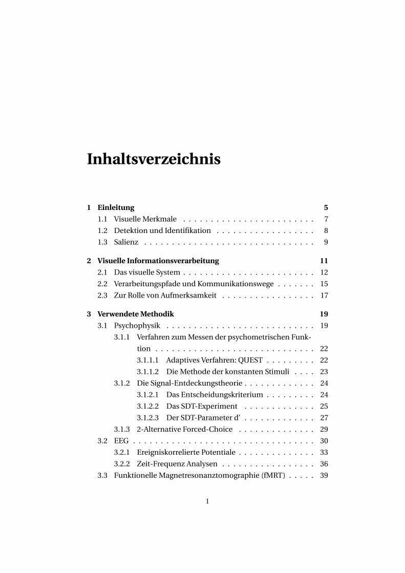
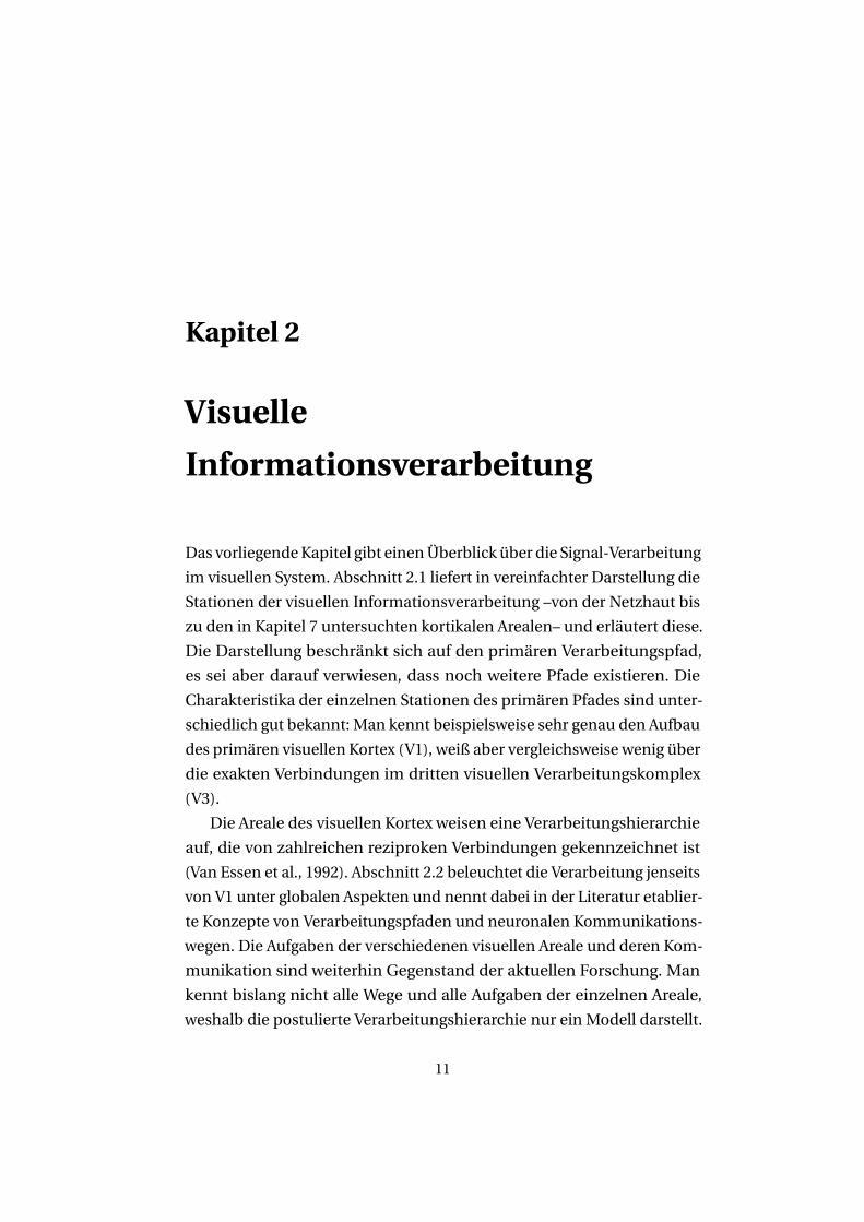
Abbildung 2.1:Der Weg der visuellen Information und Lage der visuellenAreale (verändert nach Logothetis, 2002). (A) Gesamtdarstellung. (B) Pri-märer visueller Pfad. (C) Lage der visuellen Areale in der Innenansicht derrechten Hemisphäre (Sagittalschnitt).
beitungsfunktionen zugesprochen, da es auch nicht-retinale Eingänge,
sowie Querverbindungen innerhalb der Schichten hat (Kastner et al.,
2006; Sherman, 2007; Suder & Worgotter, 2000). Vom CGL aus ziehen die
Axone der Neurone als „Radiatio Optica” (Sehstrahlung) zu V1 (siehe Abb.
2.1A und B).
Die Verarbeitung in V1 ist funktionell säulenartig organisiert (Kan-
del et al., 2000, S. 532 ff.). Eine Säule ist ein kleiner Bereich des Kortex
(inklusive der darunter senkrecht zur Oberfläche liegenden sechs Schich-
ten), dessen Neurone Information über einen definierten Bereich in der
Außenwelt (dem sogenannten rezeptiven Feld) kodieren. In V1 werden
13
KAPITEL 2. VISUELLE INFORMATIONSVERARBEITUNG
in diesen Säulen Information über Orientierung, Farbe, Bewegung und
binokuläre Interaktion (Stereopsis) kodiert. Die Anordnung der Säulen
zueinander entspricht den Rezeptorbeziehungen auf der Retina, d.h. be-
nachbarte Orte auf der Retina sind auch in V1 (und im CGL) benachbart.
Man nennt diese Ordnung retinotop (Tootell et al., 1982). Da die Rezep-
tordichte auf der Retina, wie oben erwähnt, unterschiedlich ist, sind
auch verschiedene Bereiche der Retina dementsprechend unterschied-
lich stark in V1 ausgeprägt. So ist die Fovea im Verhältnis zur Größe des
Bereichs, den sie in der Außenwelt kodiert, überrepräsentiert (vgl. Abb.
3.9). Die Repräsentationen des oberen und unteren Gesichtsfeldes sind in
V1 an einer anatomischen Einfaltung des Kortex, der „Fissura Calcarina”
getrennt: Anatomisch gesehen oberhalb (dorsal) der Fissura Calcarina
liegt die Repräsentation des unteren Gesichtsfeldes, wohingegen unter-
halb (ventral) die Repräsentation des oberen Gesichtsfeldes liegt. Die
sich jeweils zu beiden Seiten anschließenden dorsalen und ventralen
Teile der Areale V2 und V3 enthalten ebenfalls Repräsentationen nur des
unteren bzw. des oberen Gesichtsfeldes (siehe Abb. 2.1A und C). Erst
beide Teile dieser Areale bilden gemeinsam das gesamte Gesichtsfeld ab.
Im Folgenden wird diese zusätzliche Unterteilung vernachlässigt. Die
Areale V3A (eine funktionale Untereinheit von V3) und V4 enthalten dann
wieder vollständige Repräsentationen der jeweiligen Gesichtsfeldhälfte
(McKeefry & Zeki, 1997; Tootell et al., 1997), getrennt in linker und rechter
Hemisphäre.
Das Areal V2 wird als Schnittstelle zwischen V1 und dem restlichen
visuellen Kortex angesehen (Sincich & Horton, 2002), da ein Großteil
der aus V1 kommenden Neurone V2 innerviert. Somit integriert V2 In-
formation aus V1. Es ist funktionell und anatomisch gut geeignet, um
entscheidend an Figur-Grund Unterscheidungsprozessen beteiligt zu
sein (Shipp & Zeki, 2002a,b). Gestützt wird diese Ansicht durch den Be-
fund, dass Neurone in V2 zeitlich vor V1 auf Scheinkonturen reagieren
(Ffytche & Zeki, 1996; Lee & Nguyen, 2001).
Das sich an V2 anschließende Areal V3 (ventral auch als VP bezeich-
net) wird auf der dorsalen Seite mit der Verarbeitung von globaler Bewe-
14
2.2. VERARBEITUNGSPFADE UND KOMMUNIKATIONSWEGE
gung in Verbindung gebracht (Braddick et al., 2001; Moutoussis & Zeki,
2008; Tootell et al., 1998), sowie auf der ventralen Seite mit der Verar-
beitung von Form- und Tiefeninformation (Georgieva et al., 2009). Die
genaue funktionelle Bedeutung von V3 ist allerdings weitgehend unbe-
kannt, da es hohe interindividuelle Unterschiede in den Größen von V3
gibt und auch zahlreiche Primaten bekannt sind, bei denen man kein
homologes Areal gefunden hat (Kaas, 1996; Kaas & Lyon, 2001). Auf der
ventralen Seite schließt sich Areal V4 an (siehe Abb. 2.1A und C), wel-
ches eine große Rolle bei der Verarbeitung von Farben und komplexen
Formen spielt (McKeefry & Zeki, 1997; Pasupathy & Connor, 2002; Zeki,
1973, 1980). Das klassische Areal für die Auswertung von Bewegung ist
V5 (auch bezeichnet als MT – Zeki, 1974; Zeki et al., 1991). Bis zu diesem
Punkt ist die retinotope Ordnung weitgehend erhalten geblieben. Auch
die Trennung zwischen linkem und rechten Gesichtsfeld ist noch vor-
handen, allerdings gibt es bereits in V1 Querverbindungen in die andere
Hemisphäre, so dass sich die visuellen Areale beider Hemisphären auch
gegenseitig beeinflussen.
Die weitere Spezialisierung der in der Hierarchie noch höher liegen-
den Areale geht einher mit einer Abnahme der retinotopen Ordnung. So
reagieren Areale im „Lateral Occipital Complex” (LOC) auf das Vorhan-
densein von Objekten, relativ unabhängig davon, wo sie im Gesichtsfeld
auftauchen (Malach et al., 1995).
2.2 Verarbeitungspfade und Kommunikationswege
Die Verarbeitungswege im visuellen System wurden überschaubarer
durch das Postulat zweier von V1 wegführender Pfade, den dorsalen
und den ventralen Pfad (Mishkin et al., 1983). Funktionell wurden diesen
Pfaden unterschiedliche Bedeutungen zugeteilt: Im dorsalen Pfad (in
Abb. 2.1 von V1 in Richtung V3A) wird die räumliche Lage von Objek-
ten ausgewertet, wohingegen der ventrale Pfad (in Abb. 2.1 von V1 in
Richtung V4) die Objekte an sich verarbeitet. Die oben erwähnten objekt-
sensitiven Areale des LOC gehören beispielsweise zum ventralen Pfad.
Neuere Studien erweitern dieses Konzept, indem sie zeigen, dass Objekte
15
KAPITEL 2. VISUELLE INFORMATIONSVERARBEITUNG
im dorsalen Pfad in egozentrischen (d.h. auf die Position des Individu-
ums zentrierten) Koordinaten repräsentiert sind, wohingegen Objekte im
ventralen Pfad in allozentrischen (d.h. auf das Objekt selbst zentrierten)
Koordinaten repräsentiert sind (Carey et al., 2006; Schenk, 2006). Der
dorsale Pfad führt hin zum somatosensorischen undmotorischen Kortex,
was ein weiterer Hinweis darauf sein könnte, dass im dorsalen Pfad die
handlungsrelevante, eben auf das Individuum zentrierte, Information
verarbeitet wird. Um die Kommunikationswege entlang dieser Pfade bes-
ser verstehen zu können, werden im Folgenden kurz deren Prinzipien
auf der Ebene einzelner Zellen bzw. Areale behandelt.
In vielen kortikalen Arealen finden sich oftmals Zellen mit unter-
schiedlichen Antworteigenschaften innerhalb des gleichen Areals. Bei-
spielsweise reagieren in V1 verschiedene Zellen auf Orientierungs- und
Farbinformation. Diese Unterschiede auf gleicher hierarchischer Ebene
führten zu der Ansicht, dass das visuelle System Information parallel aus-
wertet, also z.B. Orientierungs-, Farb- undTiefeninformation unabhängig,
nebeneinander und gleichzeitig verarbeitet werden (Hubel & Livingstone,
1987; Lennie, 1980; Livingstone &Hubel, 1988; Merigan &Maunsell, 1993;
Zeki, 1978). Die Filterung von Signalen, sowie deren spezialisierte Auswer-
tung sind wesentliche Prinzipien der visuellen Verarbeitung. Allerdings
ist eine strikte Trennung verschiedener Subsysteme unwahrscheinlich,
da es innerhalb nahezu aller Stufen Interaktionen zwischen Neuronen,
sowie in der Hierarchie vorwärts- und rückwärtsgerichtete Verbindungen
zwischen visuellen Arealen gibt (Van Essen et al., 1992). So hat beispiels-
weise V1 auch direkte Hin- und Rückprojektionen zu V3 oder V4. Das
visuelle Signal steigt also nicht, ähnlich einer Treppe, in der Hierarchie
Stufe um Stufe hinauf, sondern es wird permanent zwischen und inner-
halb der Stufen interagiert. Trotzdem unterliegt diese Interaktion einer
strengen Ordnung, die aber bislang nur in Teilen verstanden ist.
Die Wege der neuronalen Kommunikation werden auf der Ebene der
(z.B. visuellen) Areale folgendermaßen klassifiziert: Neurone, die inner-
halb eines Areals kommunizieren, interagieren „lateral”. Wird ein Signal
in der Verarbeitungshierarchie aufsteigend weitergeleitet, so spricht man
16
2.3. ZUR ROLLE VON AUFMERKSAMKEIT
von einem „bottom-up” Signal (übersetzt: von unten nach oben). Dem-
gegenüber steht das „top-down” Signal (übersetzt: von oben nach unten),
in dem die Signalleitung von einem hierarchisch höher gelegenen Areal
zu einem niedrigeren Areal verläuft. In diesem Zusammenhang steht
das Konzept vom Zusammenspiel externer und interner Faktoren: Eine
sensorische, von externen Reizen getriebene neuronale Aktivität verur-
sacht das bottom-up Signal, wohingegen interne Zustände das top-down
Signal verursachen und bestimmen, wie bottom-up Signale verarbeitet
werden. Im Hinblick auf die Salienz eines Reizes gibt es also bottom-up
Signale, welche durch den Reiz selbst ausgelöst werden, sowie top-down
Signale, die z.B. von der Aufgabenstellung beeinflusst werden. Teilwei-
se werden die Begriffe „feedforward” (übersetzt: vorwärtsgerichtet) und
„feedback” (übersetzt: Rückkopplung) im Kontext der Kommunikation
zwischen Arealen als Synonyme für bottom-up und top-down verwendet
(Lamme et al., 1998; Lamme & Roelfsema, 2000).
Das Konzept der Aufmerksamkeit stellt einen der wichtigsten top-
down Einflüsse auf die visuelle Informationsverarbeitung dar und wird
daher im folgenden Abschnitt näher beleuchtet.
2.3 Zur Rolle von Aufmerksamkeit
Im alltäglichen Sprachgebrauch wird dasWort Aufmerksamkeit u.a. als
Synonym für Wachsamkeit, Teilnahme und Sorgfalt benutzt. Manmuss
sich also auf etwas konzentrieren, um aufmerksam zu sein und damit
anderes vernachlässigen. Auch unser Gehirn filtert und selektiert perma-
nent Information, um ein optimales Verhalten zu ermöglichen. Auf das
visuelle System bezogen bedeutet das: Wenn wir basierend auf visuel-
ler Information handeln wollen, können wir nicht immer die gesamte
Information verarbeiten undmüssen daher unsere Aufmerksamkeit auf
etwas Bestimmtes richten. Diese kontextabhängige Selektion der visu-
ellen Information bezeichnet man als den Prozess der Aufmerksamkeit
(Wolfe, 2000). Allerdings sei darauf verwiesen, dass es unterschiedliche
Definitionen von Aufmerksamkeit gibt, da dieser Begriff für viele, z.T.
17
KAPITEL 2. VISUELLE INFORMATIONSVERARBEITUNG
verschiedene Aspekte verwendet wird (für eine ausführliche Diskussion
des Begriffes siehe Pashler, 1999, S. 1 ff.).
Der oben genannte Selektionsprozess ist auf der neuronalen Verarbei-
tungsebene ein top-down Einfluss auf bottom-up Information (Maunsell
& Treue, 2006; Treue, 2003). Das visuelle System nimmt also nicht einfach
passiv die Information auf, sondern es filtert und selektiert (Heeger &
Ress, 2004). Bezüglich dieser Selektion können räumliche (Assad, 2003;
Reynolds & Chelazzi, 2004; Yantis & Serences, 2003), Objekt-basierte
(O’Craven et al., 1999; Scholl, 2001) undMerkmals-basierte Aufmerksam-
keitseffekte (Corbetta et al., 1990; Maunsell & Treue, 2006) unterschieden
werden. Die räumliche Aufmerksamkeit liegt, ähnlich einem Scheinwer-
fer, auf einem bestimmten Ort des Gesichtsfeldes. Jede visuelle Infor-
mation, die innerhalb dieses Scheinwerfers liegt, wird stärker gewichtet
als Information außerhalb. Bei der Objekt-basierten Aufmerksamkeit
wird das Objekt selbst stärker gewichtet als andere Objekte, wohingegen
bei der Merkmals-basierten Aufmerksamkeit nur die Verarbeitung des
Merkmals gewichtet wird.
Durch die oben genannten Definitionen von Aufmerksamkeit wird
unmittelbar klar, dass Aufmerksamkeit auch die Salienz eines Objekts be-
einflusst. Steht das Objekt im Fokus eines Aufmerksamkeitsprozesses (z.B.
durch seinen Ort, seine Merkmale oder weil das Objekt selbst relevant
ist), so wird es deutlich salienter sein, als wenn es nicht in diesem Fokus
liegt. Um diese Effekte zu berücksichtigen, wurde in den Studien dieser
Arbeit versucht, die Bedingungen für den Einfluss von Aufmerksamkeit
jeweils konstant zu halten.
18
Kapitel 3
VerwendeteMethodik
Im folgenden Kapitel werden die Grundlagen der in dieser Arbeit ver-
wendetenMethoden kurz erläutert. Die drei Abschnitte –Psychophysik,
Elektrophysiologie und funktionelle Magnetresonanztomographie– be-
schreiben die Methodik nur insoweit, wie es für das Verständnis der drei
Studien (Kapitel 5, 6 und 7) notwendig ist.
3.1 Psychophysik
Die Messung vonWahrnehmungsleistungen auf der Basis des Verhaltens
stellt die zugleich intuitivste und indirekteste Methode dar. Die große
Schwierigkeit liegt hierbei in der Frage, wie man die subjektive Empfin-
dung jedes Einzelnen charakterisieren kann, um schließlich generelle
Aussagen über die Wahrnehmung treffen zu können. Eine Antwort hier-
für liefert die Psychophysik, die versucht, den scheinbarenWiderspruch
zu lösen, subjektive Empfindung objektiv messbar zu machen. Gewis-
sermaßen Vater der Psychophysik ist Gustav Fechner (1801-1887), der
diese 1860 in seinemWerk „Elemente der Psychophysik“ begründete. Er
definiert die Psychophysik als die Lehre von der Beziehung „zwischen
körperlicher und geistiger, physischer und psychischer, Welt“ (Fechner,
1860, S. 8).
Ausgangspunkt der Psychophysik ist die Tatsache, dass unsere Wahr-
nehmung nicht exakt physikalische Verhältnisse widerspiegelt. Bereits
19
KAPITEL 3. VERWENDETE METHODIK
vor Fechner stellte Ernst Heinrich Weber (1795-1878) fest, dass unsere
Wahrnehmung vom Kontext abhängig ist. Nimmtman ein Gewicht von
1 g in die eine und eines von 2 g in die andere Hand, so wirdman leicht sa-
gen können, welches Gewicht schwerer wiegt. Macht man denselben Ver-
such aber mit 101 g und 102 g, so wird man es nicht mehr sagen können,
denn beides wird sich gleich schwer anfühlen. Die Physik misst in bei-
den Fällen einen Unterschied von 1g, unsere Wahrnehmung allerdings
nimmt eher prozentuale Unterschiede wahr. Weber untersuchte daher
gerade wahrnehmbare Unterschiede (engl. just noticeable differences)
unserer Sinne. Offensichtlich muss eine äußere physikalische Größe ei-
neWahrnehmungsschwelle überschreiten, um von uns überhaupt erst
bemerkt zu werden. Das Messen dieser Wahrnehmungsschwellen ist bis
heute einer der Schwerpunkte der Psychophysik. Fechner unterteilte
die Wahrnehmungsschwellen in Reiz- und Unterschiedsschwellen. Die
Reizschwelle ist der absolute Mindestwert, ab dem überhaupt innerhalb
der betrachteten Sinnesmodalität wahrgenommen werden kann. Zur
Beschreibung der Reizschwelle schreibt Fechner für das Hören: „So hö-
ren wir eine zu ferne Glocke nicht mehr. Sollten aber 100 Glocken, deren
keine wir einzeln hören, in derselben Ferne zusammen lauten, so würden
wir sie hören. Also muss doch auch jede einzelne Glocke in dieser Ferne
ihren Beitrag zum Hören geben (...)“ (Fechner, 1860, S. 242). Die Unter-
schiedsschwelle hingegen betrachtet den Punkt, ab demman in der Lage
ist, zwei Reize voneinander zu trennen. Das oben erwähnte Beispiel zur
Unterscheidung von Gewichten beschreibt auch das Wesen der Unter-
schiedsschwelle. Diese ist im ersten Fall (1 g gegenüber 2 g) überschritten
und im zweiten Fall (101 g gegenüber 102 g) unterschritten.
Das Konzept einer Wahrnehmungsschwelle suggeriert, dass es einen
festen Punkt in der Reizintensität gibt, ab dem der Reiz von nicht wahr-
nehmbar aufwahrnehmbar springt (illustriert in Abb. 3.1B). Tatsächlich
aber hat die gemessene Beziehung zwischen Reizintensität und Wahr-
nehmung den Charakter einer sigmoiden Funktion, d.h. es gibt keinen
diskreten Übergang, sondern einen Bereich, in dem die Wahrnehmung
(gemessen als Detektionsleistung) langsam ansteigt. Diese gemessene
20
3.1. PSYCHOPHYSIK
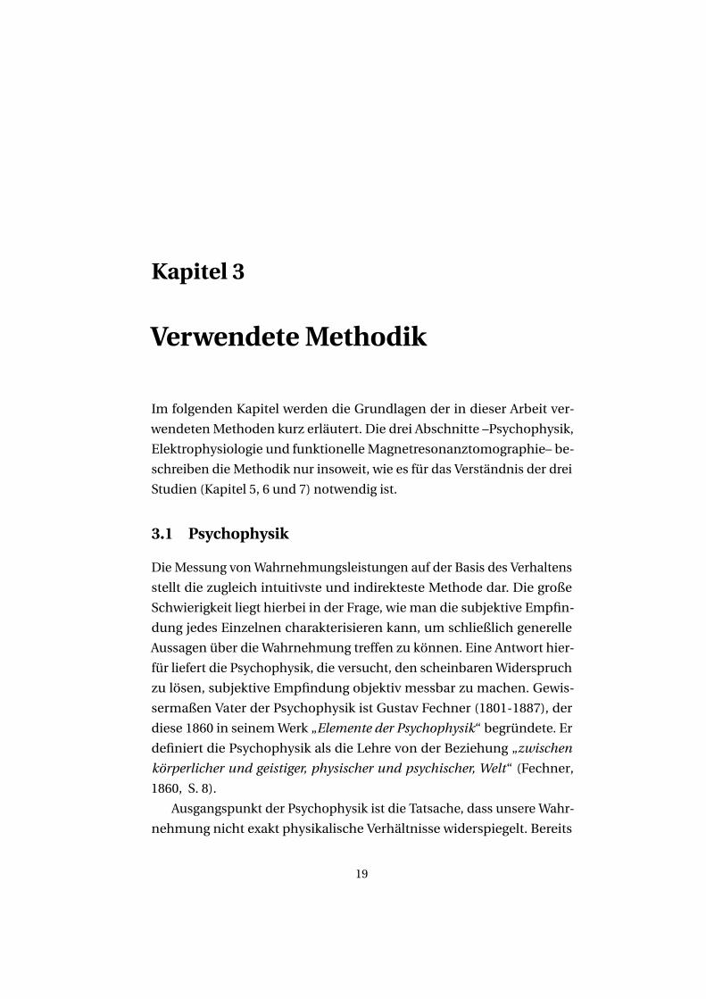
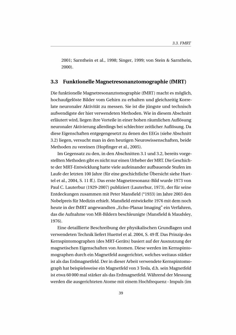
Abbildung 3.1: Psychometrische Funktionen. (A) Rot markiert ist dieSchwelle (hier Detektionsleistung von 50%) einer psychometrischenFunktion (durchgezogene Linie). Die gestrichelten Linien illustrieren dieVeränderung der Funktion bei Verschiebung der Steigung (�) oder der La-ge desWendepunktes (μ). Eine Änderung der Steigung alleine ändert nichtden Schwellenwert, wohingegen eine Verschiebung desWendepunktesauch die Schwelle verschiebt. (B) Ideale Schwellenfunktion, d.h. es erfolgtentweder keine oder zu 100% erfolgreiche Detektionen.
Beziehung zwischen Reizintensität und Wahrnehmung nennt man psy-
chometrische Funktion (dargestellt in Abb. 3.1A). Man misst die psycho-
metrische Funktion über mehrere „Versuchsdurchgänge” (engl. trials).
Hierbei wird einer Versuchsperson der Reiz bei verschiedenen Intensi-
täten gezeigt, und sie muss wiederholt die gestellte Aufgabe lösen (z.B.
angeben, ob der Reiz da war). Für jede Reizintensität berechnet man nun
den Anteil richtiger Antworten und trägt die beiden Werte, wie in Abb.
3.1, gegeneinander auf. Die psychometrische Funktion ist dann gekenn-
zeichnet durch einen prozentualen Anstieg der richtigen Antworten und
die Schwelle ist definiert als der Intensitätswert, bei dem die Versuchsper-
son den Zielreiz in 50% der Fälle entdecken kann (siehe Abb. 3.1). Auch
andere Schwellendefinitionen sind möglich, werden aber nicht weiter
ausgeführt, da sie hier nicht verwendet werden. Im Folgenden werden
die in dieser Arbeit angewandten Verfahren vorgestellt, mit denenman
21
KAPITEL 3. VERWENDETE METHODIK
die psychometrische Funktion messen kann. Diese Methoden gründen
sich auf die von Fechner vorgeschlagenenMethoden zur Messung von
Wahrnehmungsschwellen.
3.1.1 Verfahren zumMessen der psychometrischen Funktion
Die psychometrische Funktion ermittelt man, indemman die Funktion
durch die gemessenen Daten legt (engl. fit). Da man die Parameter der
tatsächlichen (d.h. dem Prozess unterliegenden) Funktion nicht kennt,
benutzt man eine Modellfunktion (wie z.B. die in Abb. 3.1 dargestellte
Funktion). Dieses Problem haben auch alle Verfahren, mit denen man
psychometrische Funktionen misst (für eine ausführliche Diskussion
siehe Macmillan & Creelman, 2005, S. 273 ff.). Es wird immer eine vorher
definierte Modellfunktion benutzt, deren Parameter für die Repräsentati-
on der Daten angepasst werden.
3.1.1.1 Adaptives Verfahren: QUEST
Die „Quick Estimation by Sequential Testing“ (QUEST – übersetzt: schnel-
le Schätzung durch sequentielles Testen) gehört zu den adaptiven Stairca-
se Verfahren (engl. Treppenstufe). Diese haben sich aus der von Fechner
vorgeschlagenen „Methode der richtigen und falschen Fälle” entwickelt
(Fechner, 1860, S. 71 ff.). Das Prinzip der adaptiven Staircase (für eine
Übersicht siehe Treutwein, 1995) beginnt mit einem Startwert für die
Reizintensität. Die Versuchsperson versucht nun, die gestellte Aufgabe
zu lösen (z.B. „War der Reiz links oder rechts?”). In Abhängigkeit von
der Antwort ändert der Staircase-Algorithmus nun die Reizintensität. Bei
falscher Antwort wird die Intensität erhöht, bei richtiger Antwort wird
sie verringert. Auf diese Art nähert man sich schrittweise der gesuchten
Schwelle auf der psychometrischen Funktion.
Bei der QUEST-Strategie (Watson & Pelli, 1983) wird von vornherein ei-
ne bestimmte psychometrische Funktion benutzt und auf deren Schwel-
lenwert getestet. Die hierbei angenommene psychometrische Funktion
(z.B. die Sigmoidfunktion) ist eindeutig durch Wendepunkt und Steigung
beschrieben. In Abhängigkeit von der Antwort werden nun der geschätz-
22
3.1. PSYCHOPHYSIK
te Wendepunkt und die Steigung neu ermittelt und es wird wiederum
auf dem resultierenden Schwellenwert getestet. Man erhält nach dem
letzten Versuchsdurchlauf den Wendepunkt und die Steigung der zu ver-
wendenden Funktion nach dem zuletzt getesteten Wert. In Ergänzung
der ursprünglichen QUEST-Strategie, stammen die Schwellen- und Stei-
gungswerte in der vorliegenden Arbeit aus einer post-hoc Analyse des
gesamten Versuchs. Diese Erweiterung wurde auch schon von Watson
& Pelli (1983) vorgeschlagen, da sie den Vorteil hat, dass der gesamte
Versuchsverlauf miteinbezogen wird.
Die Verwendung der QUEST-Strategie ist sehr effizient in der Ermitt-
lung der gesuchten Schwelle, daher werden nur relativ wenige Versuchs-
durchgänge benötigt (etwa 50-100). Mit QUEST wird sehr schnell auf
der tatsächlichen Schwelle getestet, daher ist dieses Verfahren nicht so
genau bezüglich der Bestimmung der Steigung der psychometrischen
Funktion. Um diese Genauigkeit zu erhöhen, wurde in der vorliegenden
Arbeit zusätzlich die „Methode der konstanten Stimuli” angewandt.
3.1.1.2 DieMethode der konstanten Stimuli
Das heute als „Methode der konstanten Stimuli” (engl. Method of Con-
stant Stimuli) bekannte Verfahren, wurde von Fechner als die „Methode
der mittleren Fehler” (Fechner, 1860, S. 71 ff.) eingeführt. Im Gegensatz
zu adaptiven Verfahren wird bei dieser Methode auf feststehenden In-
tensitätswerten getestet. Diese werden nicht von einem Rechenalgorith-
mus ermittelt, sondern vom Experimentator vorgegeben und wieder-
holt in zufälliger Reihenfolge präsentiert. Die Reizintensitäten sollten so
gewählt sein, dass sie sowohl überschwellige als auch unterschwellige
Werte enthalten und auf dem Anstieg der psychometrischen Funktion,
d.h. zwischen den beiden Extrema 0% und 100% Detektionsleistung
(Abb. 3.1), liegen. Man wählt also z.B. fünf Werte (zwei über der Schwelle,
die Schwelle selbst und zwei unter der Schwelle), präsentiert sie jeweils
50 mal in zufälliger Reihenfolge, und wertet am Schluss aus, wie oft die
Versuchsperson auf jedemWert richtig geantwortet hat (man erhält ei-
ne Prozentzahl richtiger Antworten). Durch die erhaltenen fünf Werte
23
KAPITEL 3. VERWENDETE METHODIK
legt man die psychometrische Funktion (vgl. Abb. 3.1) und erhält somit
Wendepunkt und Steigung.
Die Anwendung dieser Methode ist nur sinnvoll, wenn man vorher
ungefähr abschätzen kann, wo die Schwelle liegt. Die Versuchsreihen dau-
ern deutlich länger (Watson & Fitzhugh, 1990), als beispielsweise bei der
QUEST-Strategie (im obigen Beispiel bräuchte man 250 Versuchsdurch-
gänge), aber, falls man die Intensitätswerte geschickt wählt, erhält man
eine genauere Bestimmung des Anstiegs der psychometrischen Funktion.
Ummöglichst genaue psychometrische Funktionen zu erhalten, wur-
de in beiden EEG-Studien (Kapitel 5 und 6) erst die Schwelle mit der
QUEST-Strategie bestimmt und dann auf der von QUEST vorhergesagten
psychometrischen Funktion die Steigung mit der „Methode der konstan-
ten Stimuli” nachgemessen.
3.1.2 Die Signal-Entdeckungstheorie
Die Signal-Entdeckungstheorie (engl. Signal Detection Theory, abgekürzt
SDT) beinhaltet einen neueren psychophysikalischen Ansatz, um Detek-
tionsleistung zu messen. Im Jahre 1966 veröffentlichten David M. Green
und John A. Swets das Buch „Signal Detection Theory and Psychophy-
sics”, in dem sie das einheitliche Schwellenkonzept durch zwei Prozesse
ersetzten: einen unveränderlichen sensorischen Prozess und einen strate-
gischen Entscheidungsprozess. Sie charakterisierten die Versuchsperson
als einen „Betrachter” (engl. observer) mit dem Ziel, sich optimal in einer
Umgebung unvorhersagbarer Variabilität zu verhalten. Auf Basis dieser
Theorie beschrieben sie experimentelle und analytischeMethoden, um
Entscheidungs- von sensorischen Faktoren zu trennen.
3.1.2.1 Das Entscheidungskriterium
Irgendwann währendmeines Studiums beschloss ich mit meiner Freun-
din, eine Nachtwanderung zu machen. Wir zogen also los, völlig naiv
ohne Taschenlampe nachts in den Wald. Anfangs ging es uns gut, wir
haben uns unterhalten und fühlten uns auch nicht unwohl, obwohl man
fast nichts sah. Mit der Zeit aber begannen wir uns gegenseitig aufzuzie-
24
3.1. PSYCHOPHYSIK
hen, links oder rechts vomWeg wäre ein Wildschwein oder ein anderes
Tier. Anfangs war das nur ein Scherz, um den Anderen zu verunsichern,
aber es führte dazu, dass wir beide extrem verunsichert waren und tat-
sächlich überall Tiere sahen. Ich bin mir bis heute sicher, dass nichts von
dem, was wir da sahen, ein Tier war.
Dieses Beispiel zeigt, dass wir nicht einfach nur automatisch auf sen-
sorische Information reagieren, sondern sie immer im Kontext wahrneh-
men. Vergleichbare visuelle Erfahrung wurde zu Beginn der Nachtwan-
derung als unkritisch betrachtet und später als Bedrohung interpretiert.
Dies stellt eine Verschiebung des Entscheidungskriteriums (engl. respon-
se bias) dar. Das Entscheidungskriterium hängt von der Situation, aber
auch von der Persönlichkeit (vorsichtig gegenüber mutig) der Versuchs-
person ab. In einem klassischen psychophysikalischen Experimentwürde
man für obiges Beispiel eine Verschiebung der Wahrnehmungschwelle
messen, ungeachtet ob sich nun die visuelle Erfahrung oder die Motiva-
tion verändert hat. Die SDT hingegen nimmt an, dass die Sensorik die
gleiche ist, und unterschiedliches Verhalten aus dem veränderten Ent-
scheidungskriterium resultiert. Gleichzeitig liefert die SDT eine Methode,
um sensorische Wahrnehmung und Entscheidungskriterium zu trennen.
Die sensorischeWahrnehmung wird hierbei durch den Parameter d ge-
kennzeichnet, das Entscheidungskriterium durch den Parameter β. Um
d und β zu berechnen, schlägt die SDT ein spezifisches experimentelles
Vorgehen vor, welches im folgenden Abschnitt erläutert wird. Die Be-
rechnung von d wird dann in Abschnitt 3.1.2.3 erklärt. Es wird gezeigt,
dass das Entscheidungskriterium im SDT-Experiment eine große Rolle
spielt, auf genaue Beschreibung seiner Berechnung wird hier allerdings
verzichtet, da es in der vorliegenden Arbeit nicht verwendet wird.
3.1.2.2 Das SDT-Experiment
Auch vor der SDTwar das Problem des Entscheidungskriteriums bekannt
(für Übersichtsartikel siehe Ehrenstein & Ehrenstein, 1999; Palmer, 2002,
S. 665 ff.). Um das Entscheidungskriterium in die Auswertung mitein-
zubeziehen, benutzte man sogenannte „Catch-Trials”, d.h. zufällig im
25
KAPITEL 3. VERWENDETE METHODIK
Zielreiz „Ja” „Nein”
korrekteErkennungen
Auslassungen
vorhanden 80 % 20 % 100 %
falsch Positive korrekteAblehnungen
nicht vorhanden 40 % 60 % 100 %
60 % 40 %
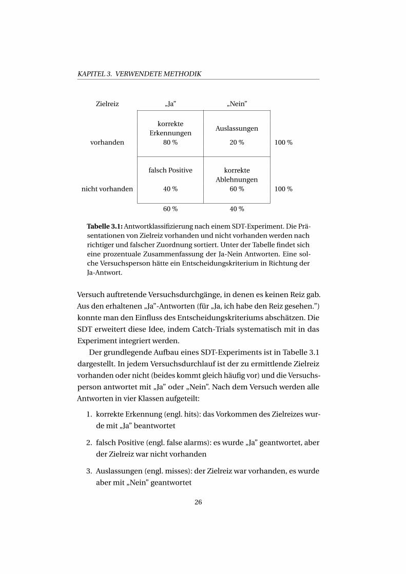
Tabelle 3.1: Antwortklassifizierung nach einem SDT-Experiment. Die Prä-sentationen von Zielreiz vorhanden und nicht vorhanden werden nachrichtiger und falscher Zuordnung sortiert. Unter der Tabelle findet sicheine prozentuale Zusammenfassung der Ja-Nein Antworten. Eine sol-che Versuchsperson hätte ein Entscheidungskriterium in Richtung derJa-Antwort.
Versuch auftretende Versuchsdurchgänge, in denen es keinen Reiz gab.
Aus den erhaltenen „Ja”-Antworten (für „Ja, ich habe den Reiz gesehen.”)
konnte man den Einfluss des Entscheidungskriteriums abschätzen. Die
SDT erweitert diese Idee, indem Catch-Trials systematisch mit in das
Experiment integriert werden.
Der grundlegende Aufbau eines SDT-Experiments ist in Tabelle 3.1
dargestellt. In jedem Versuchsdurchlauf ist der zu ermittlende Zielreiz
vorhanden oder nicht (beides kommt gleich häufig vor) und die Versuchs-
person antwortet mit „Ja” oder „Nein”. Nach dem Versuch werden alle
Antworten in vier Klassen aufgeteilt:
1. korrekte Erkennung (engl. hits): das Vorkommen des Zielreizes wur-
de mit „Ja” beantwortet
2. falsch Positive (engl. false alarms): es wurde „Ja” geantwortet, aber
der Zielreiz war nicht vorhanden
3. Auslassungen (engl. misses): der Zielreiz war vorhanden, es wurde
aber mit „Nein” geantwortet
26
3.1. PSYCHOPHYSIK
4. korrekte Ablehnungen (engl. correct rejections): der Zielreiz war
nicht vorhanden, es wurde entsprechendmit „Nein” geantwortet
Wie der folgende Abschnitt zeigt, kann man nach einer solchen Zuord-
nung der Antworten ausrechnen, wie hoch die vom Entscheidungskrite-
rium unabhängige, sensorische Wahrnehmung d ist.
3.1.2.3 Der SDT-Parameter d’
Der SDT-Parameter d ist ein Maß für die sensorisch wahrgenommene
Stärke des Zielreizes. Die SDT nimmt an, dass sensorische Systeme ver-
rauscht sind, d.h. die Entdeckung eines Eingangssignals (des Zielreizes)
wird ebenfalls mit Rauschen belegt sein. Das ist auch der Grund, weshalb
dieWiederholung eines Versuchsdurchgangs allein auf Basis sensorischer
Information zu unterschiedlichen Ergebnissen führen kann. Die Ausga-
be des Systems ist nicht von einer festen Schwelle abhängig, sondern
charakterisierbar durch Wahrscheinlichkeitsdichtefunktionen. Um so
höher die Zielreizintensität ist, um so wahrscheinlicher ist auch seine
korrekte Entdeckung. Es gibt also zwei Verteilungen der Wahrschein-
lichkeitsdichte (siehe Abb. 3.2): eine Verteilung ohne eingegangenes Si-
gnal (die Rauschverteilung) und eine Verteilung mit einem Signal (die
Signal +Rausch -Verteilung). Zur Vereinfachung nimmt man an, dass die-
se Verteilungen durchNormalverteilungen beschriebenwerden, und dass
die Varianz beider Verteilungen gleich ist. Dieser vereinfachte Fall wird als
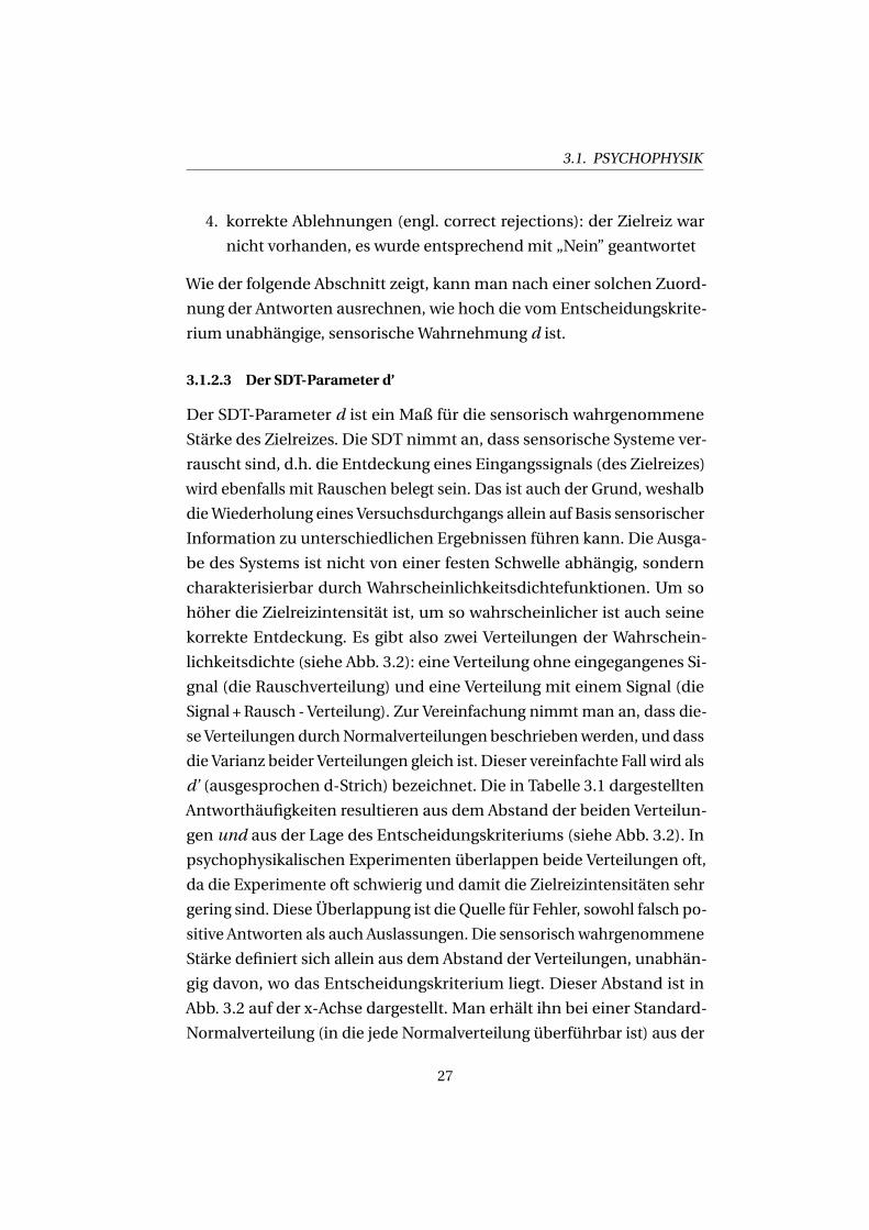
d’ (ausgesprochen d-Strich) bezeichnet. Die in Tabelle 3.1 dargestellten
Antworthäufigkeiten resultieren aus dem Abstand der beiden Verteilun-
gen und aus der Lage des Entscheidungskriteriums (siehe Abb. 3.2). In
psychophysikalischen Experimenten überlappen beide Verteilungen oft,
da die Experimente oft schwierig und damit die Zielreizintensitäten sehr
gering sind. Diese Überlappung ist die Quelle für Fehler, sowohl falsch po-
sitive Antworten als auch Auslassungen. Die sensorischwahrgenommene
Stärke definiert sich allein aus dem Abstand der Verteilungen, unabhän-
gig davon, wo das Entscheidungskriterium liegt. Dieser Abstand ist in
Abb. 3.2 auf der x-Achse dargestellt. Man erhält ihn bei einer Standard-
Normalverteilung (in die jede Normalverteilung überführbar ist) aus der
27
KAPITEL 3. VERWENDETE METHODIK
��
��������� ����������������������������������������
������������������������
����������������������������
!�" #��"
���������$%���������
$�����������
��������������������
&�����'���(�
)��
���
���
��
���
��
��
Abbildung 3.2: Wahrscheinlichkeitsdichten für Rausch-und Signal+Rausch-Verteilung. Gezeigt sind zwei Standard-Normalverteilungen. Der Parameter d’ ist definiert als der Abstandder beiden Verteilungen. Die gemessenen Antworthäufigkeiten ausTabelle 3.1 entstammen aus dem Abstand der beiden Verteilungenund der Lage des Entscheidungskriteriums. Hierbei gibt beispiels-weise die gemessene Rate korrekter Erkennungen die Fläche unterder Signal+Rausch-Verteilung bis zum Entscheidungskriterium an.Das Entscheidungskriterium liegt in dieser Abbildung etwa bei einersensorisch wahrgenommenen Intensität von 0.5, d.h. Reize links davon (<0.5) werdenmit „Nein” beantwortet, Reize rechts davon (> 0.5) mit „Ja”.
z-Transformation der gemessenen Häufigkeiten (Tabelle 3.1). Läge das
Entscheidungskriterium in Abb. 3.2 bei 0, ergäbe sich der Wert für d’ aus
der z-Transformation der korrekten Erkennungen. Liegt es nicht bei 0
(was der Normalfall ist), so muss der Abstand des Entscheidungskriteri-
ums miteinfließen. Allgemein erhält man d’ aus
d ′ = z(kor rekte Erkennungen)− z( f al schPosi t i ve) (3.1)
28
3.1. PSYCHOPHYSIK
(Green & Swets, 1988, S. 58 ff.; Macmillan & Creelman, 2005, S. 3 ff.).
Die z-Transformation überführt die entsprechende Rate in den soge-
nannten z-score, d.h. in Einheiten auf einer Standard-Normalverteilung
(Mittelwert = 0, Varianz = 1). Im Beispiel aus Tabelle 3.1 erhält man für
z(korrekte Erkennungen) = 0.84 und für z(falsch Positive) = -0.25, d.h. die
sensorische wahrgenommene Reizstärke beträgt anhand von Gleichung
3.1: d’ = 1.09.
3.1.3 2-Alternative Forced-Choice
Da in den Studien dieser Arbeit sensorische Prozesse untersucht werden,
ist das Entscheidungskriterium in allen Studien eine mögliche Störva-
riable. Eine Messmethode, um das Entscheidungskriterium direkt zu
umgehen, liefern die „Forced-Choice” Verfahren (übersetzt: erzwungene
Wahl). Auch sie haben ihre Grundlagen in der Mitte des 19. Jahrhunderts
(Bergmann, 1858, S. 88 ff.; Fechner, 1860, S. 242 ff.; für eine Übersicht sie-
he Ehrenstein & Ehrenstein, 1999). Anstatt der Versuchsperson die Wahl
zu lassen, ob sie etwas gesehen hat oder nicht, lässt man sie wählenwas
sie gesehen hat, d.h. man erzwingt eine Ja-Antwort in jedem Versuchs-
durchgang. Die Wahl kann entweder räumlicher (z.B. links oder rechts),
zeitlicher (z.B. erste oder zweite Darbietung) oder kategorialer Natur (z.B.
Hund oder Katze) sein. Das zugrundeliegende Entscheidungskriterium
gilt per Definition immer, d.h. durch den in der 2-AFC erzwungenen
Vergleich „War es dieses oder jenes?” fällt es heraus.
Bei der „2-Alternative Forced-Choice” (Abk.: 2-AFC; übersetzt: er-
zwungene Wahl mit zwei Alternativen) muss man sich zwischen zwei
Alternativen entscheiden.Wenn sich die Versuchsperson also nicht sicher
ist, muss sie raten, was bedeutet, dass eine Versuchsperson, die immer
rät, durchschnittlich 50% richtige Antworten erreicht. Dementsprechend
verläuft die psychometrische Funktion einer 2-AFC nicht zwischen 0%
und 100% (wie in Abb. 3.1), sondern zwischen 50% und 100% korrekter
Antworten. Ihr Wendepunkt liegt demnach bei 75% korrekter Antwor-
ten. Gemessene %-korrekt Antworten und d’ sind verbunden über die
29
KAPITEL 3. VERWENDETE METHODIK
Beziehung
d ′ =�2∗ z(pc) (3.2)
(Macmillan &Creelman, 2005, S. 165 ff.). Der Parameter pc steht für die ge-
messene Rate richtiger Antworten, die mit Hilfe der z-Transformation in
eine Standard-Normalverteilung überführt wird. Anhand von Gleichung
3.2 ergibt eine 2-AFCMessung auf der Schwelle ein d’ von 1.0.
Zwar fällt bei Forced-Choice Verfahren das Entscheidungskriterium
heraus, die Instruktion und Kontrolle des Versuchs ist aber dennoch
unverzichtbar. Grundvoraussetzung für ein Forced-Choice Verfahren ist,
dass die Versuchsperson tatsächlich rät, falls sie sich nicht sicher ist.
Dies sollte nach einem Versuch überprüft werden, denn of entwickeln
Versuchspersonen eine Tendenz für die Antwort, wenn sie nichts sehen
(z.B. „Wenn ich nichts sehe, sage ich immer links!”). Eine solche Strategie
führt aber zu falschenHäufigkeiten für korrekte Antworten und verfälscht
deutlich den Verlauf der psychometrischen Funktion.
3.2 EEG
1875 berichtete der englische Arzt Richard Caton (1842-1926) von elek-
trischer Spontanaktivität des Gehirns bei Hunden und Affen, die sich
in Wach- und Schlafzuständen unterscheidet und nach dem Tod nicht
mehr nachzuweisen ist. Caton erhielt seine Daten mit Elektroden, die er
auf dem intakten Gehirn oder der Schädeldecke anbrachte. Es handel-
te sich also um ein erstes Electroencephalogramm (EEG) bei Tieren. Es
sollte aber noch 50 Jahre dauern, bis das EEG beimMenschen beschrie-
ben wurde. Hans Berger (1873-1941) veröffentlichte 1929 seine Arbeit
„Über das Elektroenkephalogramm des Menschen“ und legte damit den
Grundstein für das heutige EEG. Wie zuvor Caton erkannte auch Ber-
ger, dass die gemessene elektrische Aktivität Zustände des Probanden
widerspiegelte. Im konzentrierten Zustand gab es kleine schnelle Wellen
(genannt β-Wellen), bei Entspannung gab es größere langsamere Wellen
(genannt α-Wellen). Heute wird das EEG als praktikable, nicht invasive
Methode in Medizin und Forschung vielfach (wenn auch z.T. sehr unter-
30
3.2. EEG
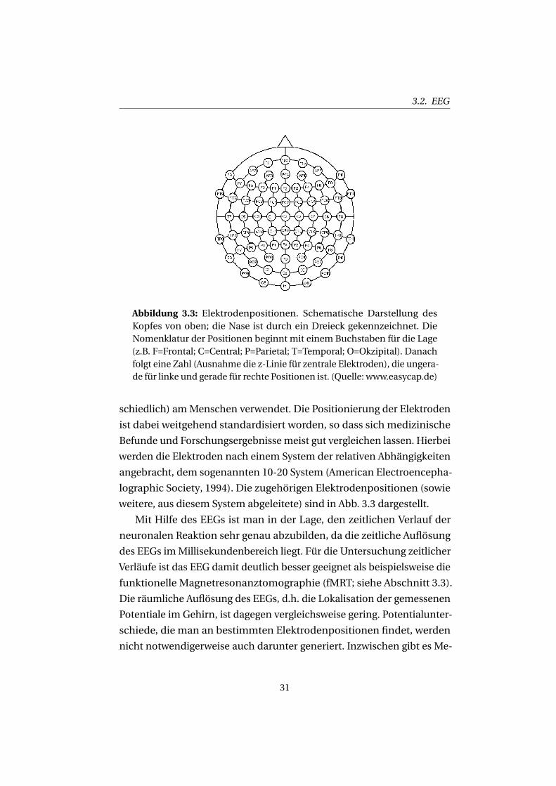
Abbildung 3.3: Elektrodenpositionen. Schematische Darstellung desKopfes von oben; die Nase ist durch ein Dreieck gekennzeichnet. DieNomenklatur der Positionen beginnt mit einem Buchstaben für die Lage(z.B. F=Frontal; C=Central; P=Parietal; T=Temporal; O=Okzipital). Danachfolgt eine Zahl (Ausnahme die z-Linie für zentrale Elektroden), die ungera-de für linke und gerade für rechte Positionen ist. (Quelle: www.easycap.de)
schiedlich) amMenschen verwendet. Die Positionierung der Elektroden
ist dabei weitgehend standardisiert worden, so dass sich medizinische
Befunde und Forschungsergebnisse meist gut vergleichen lassen. Hierbei
werden die Elektroden nach einem System der relativen Abhängigkeiten
angebracht, dem sogenannten 10-20 System (American Electroencepha-
lographic Society, 1994). Die zugehörigen Elektrodenpositionen (sowie
weitere, aus diesem System abgeleitete) sind in Abb. 3.3 dargestellt.
Mit Hilfe des EEGs ist man in der Lage, den zeitlichen Verlauf der
neuronalen Reaktion sehr genau abzubilden, da die zeitliche Auflösung
des EEGs imMillisekundenbereich liegt. Für die Untersuchung zeitlicher
Verläufe ist das EEG damit deutlich besser geeignet als beispielsweise die
funktionelle Magnetresonanztomographie (fMRT; siehe Abschnitt 3.3).
Die räumliche Auflösung des EEGs, d.h. die Lokalisation der gemessenen
Potentiale im Gehirn, ist dagegen vergleichsweise gering. Potentialunter-
schiede, die man an bestimmten Elektrodenpositionen findet, werden
nicht notwendigerweise auch darunter generiert. Inzwischen gibt es Me-
31
KAPITEL 3. VERWENDETE METHODIK
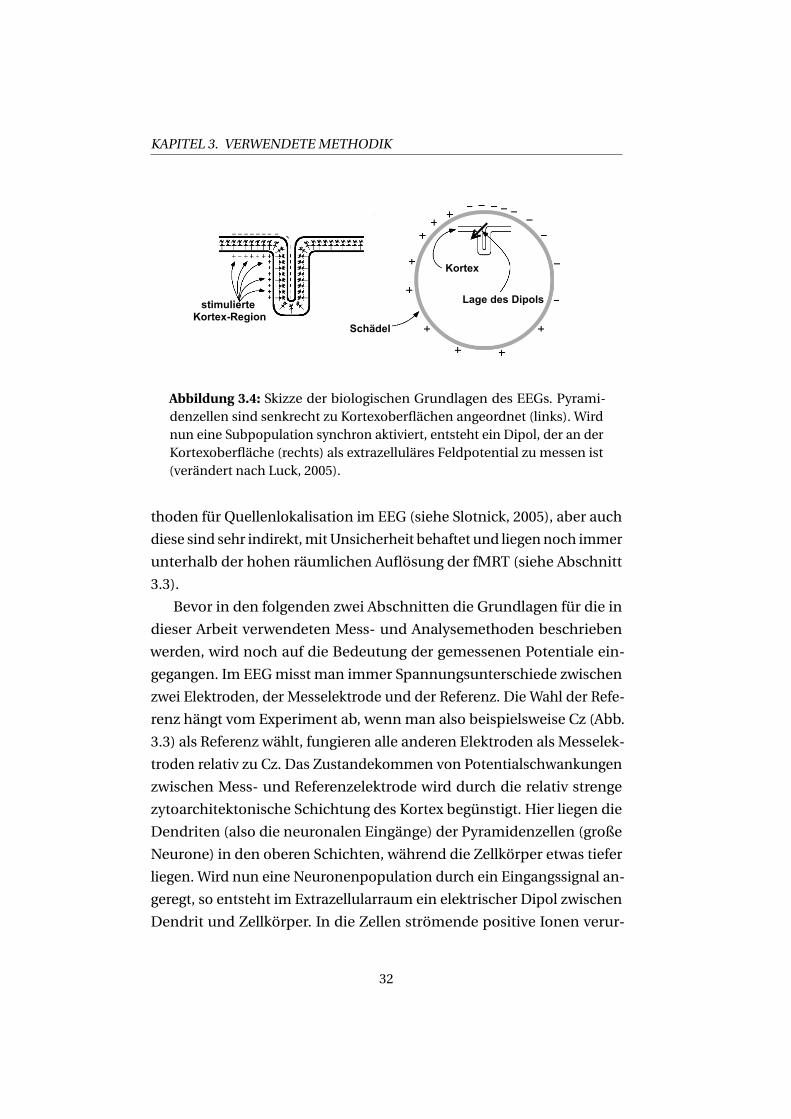
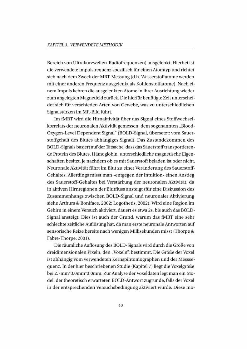
�����������*��+��� ��
�������
,� ������-�.��
*��+
Abbildung 3.4: Skizze der biologischen Grundlagen des EEGs. Pyrami-denzellen sind senkrecht zu Kortexoberflächen angeordnet (links). Wirdnun eine Subpopulation synchron aktiviert, entsteht ein Dipol, der an derKortexoberfläche (rechts) als extrazelluläres Feldpotential zu messen ist(verändert nach Luck, 2005).
thoden für Quellenlokalisation im EEG (siehe Slotnick, 2005), aber auch
diese sind sehr indirekt,mitUnsicherheit behaftet und liegennoch immer
unterhalb der hohen räumlichen Auflösung der fMRT (siehe Abschnitt
3.3).
Bevor in den folgenden zwei Abschnitten die Grundlagen für die in
dieser Arbeit verwendeten Mess- und Analysemethoden beschrieben
werden, wird noch auf die Bedeutung der gemessenen Potentiale ein-
gegangen. Im EEGmisst man immer Spannungsunterschiede zwischen
zwei Elektroden, der Messelektrode und der Referenz. Die Wahl der Refe-
renz hängt vom Experiment ab, wennman also beispielsweise Cz (Abb.
3.3) als Referenz wählt, fungieren alle anderen Elektroden als Messelek-
troden relativ zu Cz. Das Zustandekommen von Potentialschwankungen
zwischen Mess- und Referenzelektrode wird durch die relativ strenge
zytoarchitektonische Schichtung des Kortex begünstigt. Hier liegen die
Dendriten (also die neuronalen Eingänge) der Pyramidenzellen (große
Neurone) in den oberen Schichten, während die Zellkörper etwas tiefer
liegen. Wird nun eine Neuronenpopulation durch ein Eingangssignal an-
geregt, so entsteht im Extrazellularraum ein elektrischer Dipol zwischen
Dendrit und Zellkörper. In die Zellen strömende positive Ionen verur-
32
3.2. EEG
sachen im Extrazellularraum der Dendritenregion eine Negativierung
gegenüber der Zellkörperregion. Da die Pyramidenzellen außerdem noch
senkrecht zur Kortexoberfläche ausgerichtet sind, sorgt die synchrone
Aktivierung dieser Neurone für die Ausbildung eines Dipols, den man
als elektrisches Feldpotential an der Kortexoberfläche messen kann (sie-
he Abb. 3.4). Im EEG werden die Potentiale am deutlichsten gesehen,
deren Dipole möglichst direkt zwischen Mess- und Referenzelektrode
ausgerichtet sind. Die eigentlichenWährung neuronaler Kommunikati-
on, das Aktionspotential, wird im EEG nicht direkt gemessen. Stattdessen
misst man postsynaptische Aktivierung, die durch Aktionspotentiale ver-
ursacht wurde, und die ihrerseits wieder zu Aktionspotentialen führt.
3.2.1 Ereigniskorrelierte Potentiale
Ereigniskorrelierte Potentiale (EKPs) sind diejenigen Potentiale im EEG,
die spezifischmit einer Reizpräsentation zusammenhängen, d.h. die re-
lativ zeitgenau vor, während oder nach einem Reiz auftreten. Sie sind im
Roh-EEG nicht unmittelbar sichtbar, da sie von Spontanaktivität (d.h. an-
derer, nicht spezifisch von dem Reiz ausgelöster Aktivität) überlagert wer-
den. Zeigt man nun wiederholt den zu untersuchenden Reiz, so wird die
mit dem Reiz korrelierte Aktivität immer wieder im EEG auftauchen. Für
die Berechnung der EKPs braucht man nun den genauen Zeitpunkt der
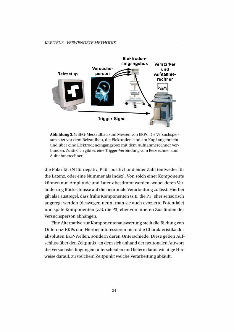
Reizpräsentation. Diesen bekommtman in einem geeigneten Messauf-
bau (siehe Abb. 3.5) durch das Trigger-Signal (übersetzt: Auslöser), das
vom Reizrechner zum EEG-Aufnahmerechner geschickt wird. Nach der
Datenaufnahme legt man einen festen Zeitbereich relativ zur Reizdarbie-
tung fest (die sogenannte Epoche, z.B. -100ms bis 500ms). Anschließend
mittelt man alle Epochen, so dass sich die nicht mit dem Reiz korre-
lierte Spontanaktivität herausmittelt. Beispielhaft ist dieser Vorgang in
Abb. 3.6 dargestellt. Das resultierende EKP enthält dann charakteristi-
sche Wellenformen, sogenannte Komponenten, die abhängig von der
untersuchten Sinnesmodalität vielfach charakterisiert sind (für Übersich-
ten siehe Fabiani et al., 2000; Key et al., 2005; Luck, 2005, S. 34 ff.). Die
Benennung dieser Komponenten verläuft nach einem Buchstaben für
33
KAPITEL 3. VERWENDETE METHODIK
Abbildung 3.5: EEG-Messaufbau zumMessen von EKPs. Die Versuchsper-son sitzt vor dem Reizaufbau, die Elektroden sind am Kopf angebrachtund über eine Elektrodeneingangsbox mit dem Aufnahmerechner ver-bunden. Zusätzlich gibt es eine Trigger-Verbindung vom Reizrechner zumAufnahmerechner.
die Polarität (N für negativ, P für positiv) und einer Zahl (entweder für
die Latenz, oder eine Nummer als Index). Von solch einer Komponente
können nun Amplitude und Latenz bestimmt werden, wobei deren Ver-
änderung Rückschlüsse auf die neuronale Verarbeitung zulässt. Hierbei
gilt als Faustregel, dass frühe Komponenten (z.B. die P1) eher sensorisch
angeregt werden (deswegen nennt man sie auch evozierte Potentiale)
und späte Komponenten (z.B. die P3) eher von inneren Zuständen der
Versuchsperson abhängen.
Eine Alternative zur Komponentenauswertung stellt die Bildung von
Differenz-EKPs dar. Hierbei interessieren nicht die Charakteristika der
absoluten EKP-Wellen, sondern deren Unterschiede. Diese geben Auf-
schluss über den Zeitpunkt, an dem sich anhand der neuronalen Antwort
die Versuchsbedingungen unterscheiden und liefern damit wichtige Hin-
weise darauf, zu welchem Zeitpunkt welche Verarbeitung abläuft.
34
3.2. EEG
/��������
/��������
�
0 1
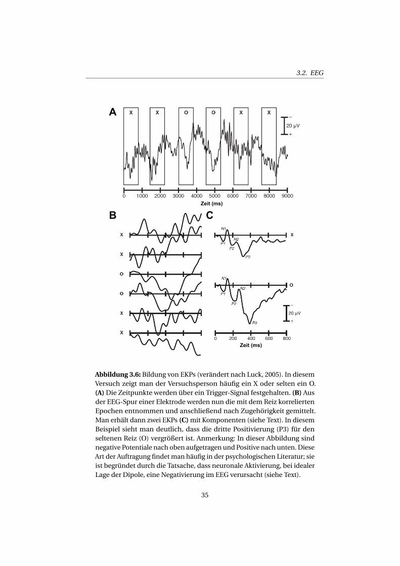
Abbildung 3.6: Bildung von EKPs (verändert nach Luck, 2005). In diesemVersuch zeigt man der Versuchsperson häufig ein X oder selten ein O.(A)Die Zeitpunkte werden über ein Trigger-Signal festgehalten. (B) Ausder EEG-Spur einer Elektrode werden nun die mit dem Reiz korreliertenEpochen entnommen und anschließend nach Zugehörigkeit gemittelt.Man erhält dann zwei EKPs (C)mit Komponenten (siehe Text). In diesemBeispiel sieht man deutlich, dass die dritte Positivierung (P3) für denseltenen Reiz (O) vergrößert ist. Anmerkung: In dieser Abbildung sindnegative Potentiale nach oben aufgetragen und Positive nach unten. DieseArt der Auftragung findet man häufig in der psychologischen Literatur; sieist begründet durch die Tatsache, dass neuronale Aktivierung, bei idealerLage der Dipole, eine Negativierung im EEG verursacht (siehe Text).
35
KAPITEL 3. VERWENDETE METHODIK
Frequenz Name (Symbol)
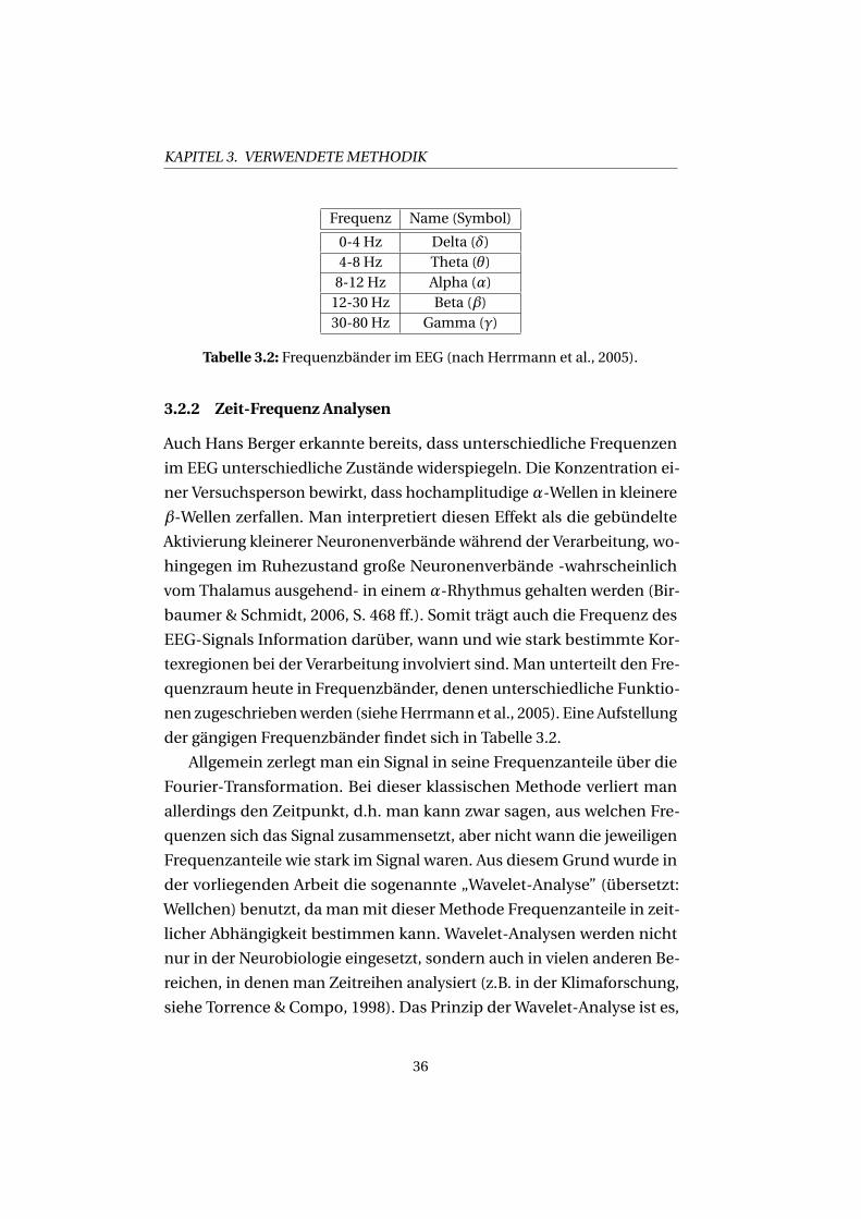
0-4 Hz Delta (δ)4-8 Hz Theta (θ)8-12 Hz Alpha (α)12-30 Hz Beta (β)30-80 Hz Gamma (γ)
Tabelle 3.2: Frequenzbänder im EEG (nach Herrmann et al., 2005).
3.2.2 Zeit-Frequenz Analysen
Auch Hans Berger erkannte bereits, dass unterschiedliche Frequenzen
im EEG unterschiedliche Zustände widerspiegeln. Die Konzentration ei-
ner Versuchsperson bewirkt, dass hochamplitudige α-Wellen in kleinere
β-Wellen zerfallen. Man interpretiert diesen Effekt als die gebündelte
Aktivierung kleinerer Neuronenverbände während der Verarbeitung, wo-
hingegen im Ruhezustand große Neuronenverbände -wahrscheinlich
vom Thalamus ausgehend- in einem α-Rhythmus gehalten werden (Bir-
baumer & Schmidt, 2006, S. 468 ff.). Somit trägt auch die Frequenz des
EEG-Signals Information darüber, wann und wie stark bestimmte Kor-
texregionen bei der Verarbeitung involviert sind. Man unterteilt den Fre-
quenzraum heute in Frequenzbänder, denen unterschiedliche Funktio-
nen zugeschriebenwerden (sieheHerrmann et al., 2005). Eine Aufstellung
der gängigen Frequenzbänder findet sich in Tabelle 3.2.
Allgemein zerlegt man ein Signal in seine Frequenzanteile über die
Fourier-Transformation. Bei dieser klassischen Methode verliert man
allerdings den Zeitpunkt, d.h. man kann zwar sagen, aus welchen Fre-
quenzen sich das Signal zusammensetzt, aber nicht wann die jeweiligen
Frequenzanteile wie stark im Signal waren. Aus diesem Grund wurde in
der vorliegenden Arbeit die sogenannte „Wavelet-Analyse” (übersetzt:
Wellchen) benutzt, da manmit dieser Methode Frequenzanteile in zeit-
licher Abhängigkeit bestimmen kann. Wavelet-Analysen werden nicht
nur in der Neurobiologie eingesetzt, sondern auch in vielen anderen Be-
reichen, in denen man Zeitreihen analysiert (z.B. in der Klimaforschung,
siehe Torrence & Compo, 1998). Das Prinzip der Wavelet-Analyse ist es,
36
3.2. EEG
zu testen, wie gut eine Funktion endlicher Dauer und definierter Fre-
quenz die Daten abbildet. Welche Funktion man dabei zugrunde legt ist
variabel und sollte von den Eigenschaften der zugrundeliegenden Daten
bestimmt werden (vgl. Samar et al., 1999). Die Wavelet-Funktion wird
in alle zu testenden Frequenzbereiche skaliert, und man testet nun an
jedem Zeitpunkt, wie gut die Funktion zu den Daten passt. Anders gesagt,
man schiebt das Wavelet über das EEG-Signal und berechnet an jedem
Punkt einen Koeffizienten, der die Ähnlichkeit von Funktion und Signal
ausdrückt. Ein Beispiel, wie man die Frequenzanteile eines EKPs mit
Hilfe einer Wavelet-Analyse darstellt, findet sich in Abb. 3.7. Analog zur
Heisenbergschen Unschärferelation, nimmt bei der Wavelet-Analyse die
zeitliche Genauigkeit mit sinkender Frequenz ab (vgl. Abb. 3.7A) und die
Genauigkeit in der Frequenz zu (nicht dargestellt). Die Wavelet-Analyse
bietet einige ergänzendeMöglichkeiten, um die EEGDaten über die EKPs
hinaus zu analysieren:
• Hohe Frequenzen werden in EKPs oftmals herausgefiltert; mit der
Wavelet-Analyse kannman gerade Effekte in hohen Frequenzen gut
nachweisen.
• Man sieht im EKP ausschließlich die zeitlich präzise, durch den
Reiz ausgelöste neuronale Aktivität, aber nicht jede Verarbeitung
im Gehirn wird mit dieser hohen zeitlichen Präzision arbeiten und
somit im EKP sichtbar sein. Mit Hilfe der Wavelet-Analyse lassen
sich gut einzelne Epochen der EEG Daten analysieren, so dass man
auch in der Lage ist, nicht zeitlich präzise auftretende Potentiale,
die sogenannten induzierten Potentiale, aufzuspüren (Herrmann
et al., 2005).
• Nach Frequenzen zerlegte Daten enthalten nicht nur Amplituden,
sondern auch Phaseninformationen. Durch Auswertung dieser In-
formation ist man in der Lage, neuronale Kommunikationswege im
Gehirn funktional sichtbar zu machen, da entfernte Gehirn-Areale
sich während ihrer Kommunikation in Phase befinden (Mima et al.,
37
KAPITEL 3. VERWENDETE METHODIK
23
43
53
33
�3�6 �566 �266 �766 �866 ��9��
�3:3
�5:3
�4:3
/��������
;�<�����=��
/��������
36�=�
56�=�
26�=� /��������266 766566
9�
36
��>
3>
�>
� 00
1
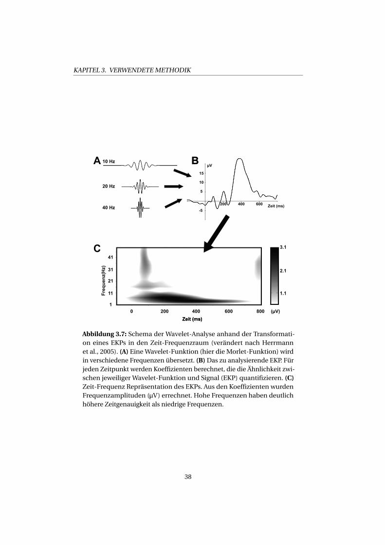
Abbildung 3.7: Schema der Wavelet-Analyse anhand der Transformati-on eines EKPs in den Zeit-Frequenzraum (verändert nach Herrmannet al., 2005). (A) EineWavelet-Funktion (hier die Morlet-Funktion) wirdin verschiedene Frequenzen übersetzt. (B)Das zu analysierende EKP. Fürjeden Zeitpunkt werden Koeffizienten berechnet, die die Ähnlichkeit zwi-schen jeweiliger Wavelet-Funktion und Signal (EKP) quantifizieren. (C)Zeit-Frequenz Repräsentation des EKPs. Aus den Koeffizienten wurdenFrequenzamplituden (μV) errechnet. Hohe Frequenzen haben deutlichhöhere Zeitgenauigkeit als niedrige Frequenzen.
38
3.3. FMRT
2001; Sarnthein et al., 1998; Singer, 1999; von Stein & Sarnthein,
2000).
3.3 Funktionelle Magnetresonanztomographie (fMRT)
Die funktionelle Magnetresonanztomographie (fMRT) macht es möglich,
hochaufgelöste Bilder vom Gehirn zu erhalten und gleichzeitig Korre-
late neuronaler Aktivität zu messen. Sie ist die jüngste und technisch
aufwendigste der hier verwendeten Methoden. Wie in diesem Abschnitt
erläutert wird, liegen ihre Vorteile in einer hohen räumlichen Auflösung
neuronaler Aktivierung allerdings bei schlechter zeitlicher Auflösung. Da
diese Eigenschaften entgegengesetzt zu denen des EEGs (siehe Abschnitt
3.2) liegen, versucht man in den heutigen Neurowissenschaften, beide
Methoden zu vereinen (Hopfinger et al., 2005).
Im Gegensatz zu den, in den Abschnitten 3.1 und 3.2, bereits vorge-
stelltenMethoden gibt es nicht nur einenUrheber derMRT. Die Geschich-
te der MRT-Entwicklung hatte viele aufeinander aufbauende Stufen im
Laufe der letzten 100 Jahre (für eine geschichtliche Übersicht siehe Huet-
tel et al., 2004, S. 11 ff.). Das erste Magnetresonanz-Bild wurde 1973 von
Paul C. Lauterbur (1929-2007) publiziert (Lauterbur, 1973), der für seine
Entdeckungen zusammen mit Peter Mansfield (*1933) im Jahre 2003 den
Nobelpreis für Medizin erhielt. Mansfield entwickelte 1976 mit dem noch
heute in der fMRT angewandten „Echo-Planar Imaging” ein Verfahren,
das die Aufnahme vonMR-Bildern beschleunigte (Mansfield &Maudsley,
1976).
Eine detaillierte Beschreibung der physikalischen Grundlagen und
verwendeten Technik liefert Huettel et al. 2004, S. 49 ff. Das Prinzip des
Kernspintomographen (des MRT-Geräts) basiert auf der Ausnutzung der
magnetischen Eigenschaften von Atomen. Diese werden im Kernspinto-
mographen durch einMagnetfeld ausgerichtet, welches weitaus stärker
ist als das Erdmagnetfeld. Der in dieser Arbeit verwendete Kernspintomo-
graph hat beispielsweise ein Magnetfeld von 3 Tesla, d.h. sein Magnetfeld
ist etwa 60 000 mal stärker als das Erdmagnetfeld. Während der Messung
werden die ausgerichteten Atomemit einemHochfrequenz - Impuls (im
39
KAPITEL 3. VERWENDETE METHODIK
Bereich von Ultrakurzwellen-Radiofrequenzen) ausgelenkt. Hierbei ist
die verwendete Impulsfrequenz spezifisch für einen Atomtyp und richtet
sich nach dem Zweck der MRT-Messung (d.h. Wasserstoffatome werden
mit einer anderen Frequenz ausgelenkt als Kohlenstoffatome). Nach ei-
nem Impuls kehren die ausgelenkten Atome in ihrer Ausrichtung wieder
zum angelegtenMagnetfeld zurück. Die hierfür benötigte Zeit unterschei-
det sich für verschieden Arten von Gewebe, was zu unterschiedlichen
Signalstärken imMR-Bild führt.
Im fMRT wird die Hirnaktivität über das Signal eines Stoffwechsel-
korrelats der neuronalen Aktivität gemessen, dem sogenannten „Blood-
Oxygen-Level Dependent Signal” (BOLD-Signal, übersetzt: vom Sauer-
stoffgehalt des Blutes abhängiges Signal). Das Zustandekommen des
BOLD-Signals basiert auf der Tatsache, dass das Sauerstoff transportieren-
de Protein des Blutes, Hämoglobin, unterschiedliche magnetische Eigen-
schaften besitzt, je nachdem ob es mit Sauerstoff beladen ist oder nicht.
Neuronale Aktivität führt im Blut zu einer Veränderung des Sauerstoff-
Gehaltes. Allerdings misst man -entgegen der Intuition- einen Anstieg
des Sauerstoff-Gehaltes bei Verstärkung der neuronalen Aktivität, da
in aktiven Hirnregionen der Blutfluss ansteigt (für eine Diskussion des
Zusammenhangs zwischen BOLD-Signal und neuronaler Aktivierung
siehe Arthurs & Boniface, 2002; Logothetis, 2002). Wird eine Region im
Gehirn in einem Versuch aktiviert, dauert es etwa 2s, bis auch das BOLD-
Signal ansteigt. Dies ist auch der Grund, warum das fMRT eine sehr
schlechte zeitliche Auflösung hat, da man erste neuronale Antworten auf
sensorische Reize bereits nach wenigenMillisekundenmisst (Thorpe &
Fabre-Thorpe, 2001).
Die räumliche Auflösung des BOLD-Signals wird durch die Größe von
dreidimensionalen Pixeln, den „Voxeln”, bestimmt. Die Größe der Voxel
ist abhängig vom verwendeten Kernspintomographen und der Messse-
quenz. In der hier beschriebenen Studie (Kapitel 7) liegt die Voxelgröße
bei 2.7mm*3.0mm*3.0mm. Zur Analyse der Voxeldaten legt man ein Mo-
dell der theoretisch erwarteten BOLD-Antwort zugrunde, falls der Voxel
in der entsprechenden Versuchsbedingung aktiviert wurde. Diese mo-
40
3.3. FMRT
dellierte Antwort nennt man die „hämodynamische Antwortfunktion”.
Ein Beispiel für Rohdaten eines Voxels und die modellierte hämodyna-
mische Antwortfunktion für eine Versuchsbedingung sind in Abb. 3.8A
dargestellt. Mit Hilfe einer statistischenMethode, dem „Allgemeinen Li-
nearenModell” (ALM), bestimmtman bei der hohen Anzahl von Voxeln
(in der in Kapitel 3.3 beschriebenen Studie besteht allein eine Aufnahme
des Gehirns aus über 150000 Voxeln) welche Voxel signifikant in der je-
weiligen Versuchsbedingung aktiviert wurden (siehe Huettel et al., 2004,
S. 336 ff.). Die Auftragung der aktivierten Voxel erfolgt gewöhnlich als
signifikanter Kontrast zwischen Versuchsbedingung und Ruhebedingung
(siehe Abb. 3.8B), bzw. zwischen zwei Versuchsbedingungen. Hierbei wer-
den die funktionellen Daten auf das Ergebnis eines anatomischen Scans
projiziert.
3.3.1 funktionelle Kartierung visueller Areale
Es steht ein einfacher Grundgedanke hinter dem Bestreben, das Gehirn
in separate Bereiche einzuteilen: Hätte man eine Karte des Gehirns, so
bräuchte man nur noch die für den jeweiligen Versuch relevanten Areale
zu untersuchen undmüsste nicht mehr das gesamte Gehirn betrachten.
Schon früh verwendete man Karten des Gehirns basierend auf anatomi-
schen und histologischen Unterschieden, wie z.B. die auch heute noch
verwendeten Karten des Neuroanatomen Korbinian Brodmann (1868-
1918). Solche Karten sind allerdings sehr grob, und nicht immer sind
anatomische und histologische Unterschiede gleichbedeutendmit funk-
tionellen Unterschieden. Die genaue Position von funktionellen Arealen
ist darüber hinaus nicht immer anatomisch exakt zu bestimmen (z.B.
ist die Lage des visuellen Areals LOC individuell sehr verschieden). Aus
diesen Gründen (und weil man die individuelle Histologie nicht kennt)
verwendet man, soweit möglich, funktionelle Karten, d.h. man macht
sich die spezifischen Eigenschaften einzelner Areale zu Nutze. So kann
man auch für das visuelle System individuelle funktionelle Karten er-
stellen, die aus einem separaten fMRT-Versuch stammen. Der konkrete
Vorteil einer vom eigentlichen Versuch unabhängigen Kartierung liegt
41
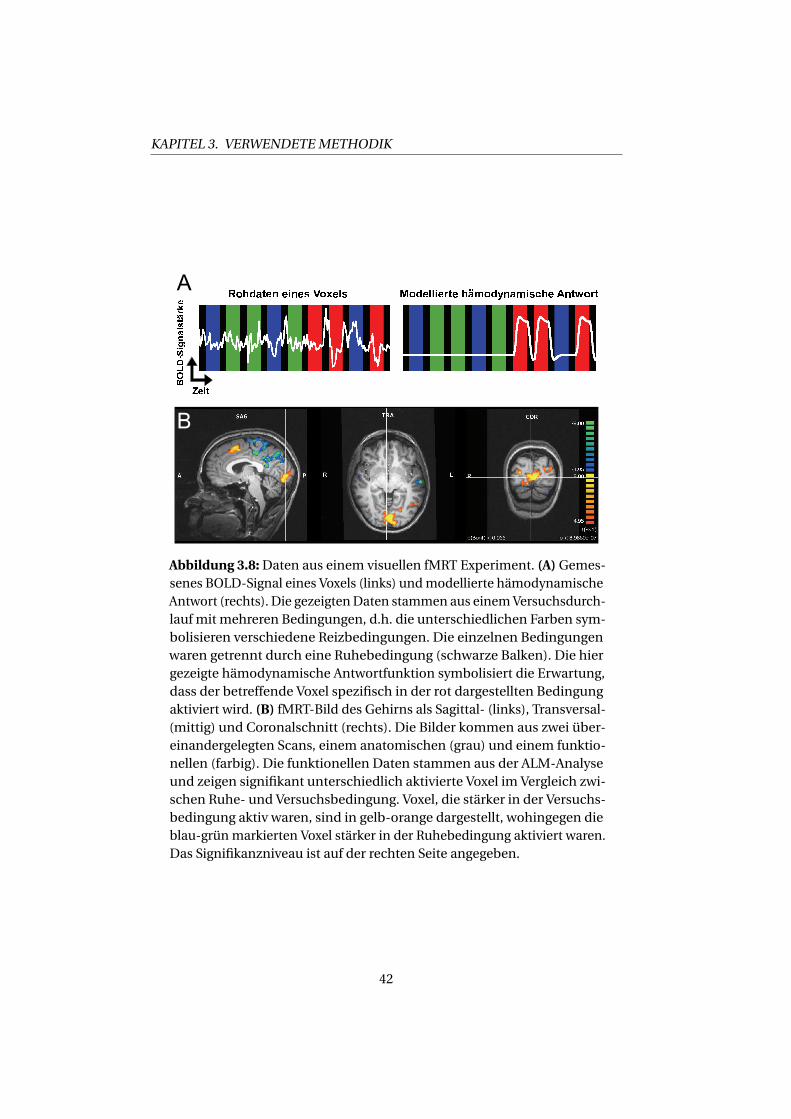
KAPITEL 3. VERWENDETE METHODIK
Abbildung 3.8:Daten aus einem visuellen fMRT Experiment. (A) Gemes-senes BOLD-Signal eines Voxels (links) undmodellierte hämodynamischeAntwort (rechts). Die gezeigtenDaten stammen aus einemVersuchsdurch-lauf mit mehreren Bedingungen, d.h. die unterschiedlichen Farben sym-bolisieren verschiedene Reizbedingungen. Die einzelnen Bedingungenwaren getrennt durch eine Ruhebedingung (schwarze Balken). Die hiergezeigte hämodynamische Antwortfunktion symbolisiert die Erwartung,dass der betreffende Voxel spezifisch in der rot dargestellten Bedingungaktiviert wird. (B) fMRT-Bild des Gehirns als Sagittal- (links), Transversal-(mittig) und Coronalschnitt (rechts). Die Bilder kommen aus zwei über-einandergelegten Scans, einem anatomischen (grau) und einem funktio-nellen (farbig). Die funktionellen Daten stammen aus der ALM-Analyseund zeigen signifikant unterschiedlich aktivierte Voxel im Vergleich zwi-schen Ruhe- und Versuchsbedingung. Voxel, die stärker in der Versuchs-bedingung aktiv waren, sind in gelb-orange dargestellt, wohingegen dieblau-grün markierten Voxel stärker in der Ruhebedingung aktiviert waren.Das Signifikanzniveau ist auf der rechten Seite angegeben.
42
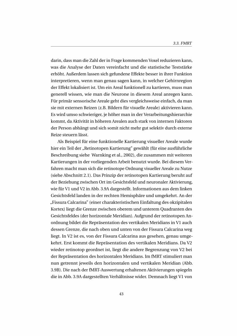
3.3. FMRT
darin, dass man die Zahl der in Frage kommenden Voxel reduzieren kann,
was die Analyse der Daten vereinfacht und die statistische Teststärke
erhöht. Außerdem lassen sich gefundene Effekte besser in ihrer Funktion
interpretieren, wenn man genau sagen kann, in welcher Gehirnregion
der Effekt lokalisiert ist. Um ein Areal funktionell zu kartieren, muss man
generell wissen, wie man die Neurone in diesem Areal anregen kann.
Für primär sensorische Areale geht dies vergleichsweise einfach, da man
sie mit externen Reizen (z.B. Bildern für visuelle Areale) aktivieren kann.
Es wird umso schwieriger, je höher man in der Verarbeitungshierarchie
kommt, da Aktivität in höheren Arealen auch stark von internen Faktoren
der Person abhängt und sich somit nicht mehr gut selektiv durch externe
Reize steuern lässt.
Als Beispiel für eine funktionelle Kartierung visueller Areale wurde
hier ein Teil der „Retinotopen Kartierung” gewählt (für eine ausführliche
Beschreibung siehe Warnking et al., 2002), die zusammenmit weiteren
Kartierungen in der vorliegenden Arbeit benutzt wurde. Bei diesem Ver-
fahren macht man sich die retinotope Ordnung visueller Areale zu Nutze
(siehe Abschnitt 2.1). Das Prinzip der retinotopen Kartierung beruht auf
der Beziehung zwischen Ort im Gesichtsfeld und neuronaler Aktivierung,
wie für V1 und V2 in Abb. 3.9A dargestellt. Informationen aus dem linken
Gesichtsfeld landen in der rechten Hemisphäre und umgekehrt. An der
„Fissura Calcarina” (einer charakteristischen Einfaltung des okzipitalen
Kortex) liegt die Grenze zwischen oberem und unterem Quadranten des
Gesichtsfeldes (der horizontale Meridian). Aufgrund der retinotopen An-
ordnung bildet die Repräsentation des vertikalen Meridians in V1 auch
dessen Grenze, die nach oben und unten von der Fissura Calcarina weg
liegt. In V2 ist es, von der Fissura Calcarina aus gesehen, genau umge-
kehrt. Erst kommt die Repräsentation des vertikalen Meridians. Da V2
wieder retinotop geordnet ist, liegt die andere Begrenzung von V2 bei
der Repräsentation des horizontalen Meridians. Im fMRT stimuliert man
nun getrennt jeweils den horizontalen und vertikalen Meridian (Abb.
3.9B). Die nach der fMRT-Auswertung erhaltenen Aktivierungen spiegeln
die in Abb. 3.9A dargestellten Verhältnisse wider. Demnach liegt V1 von
43
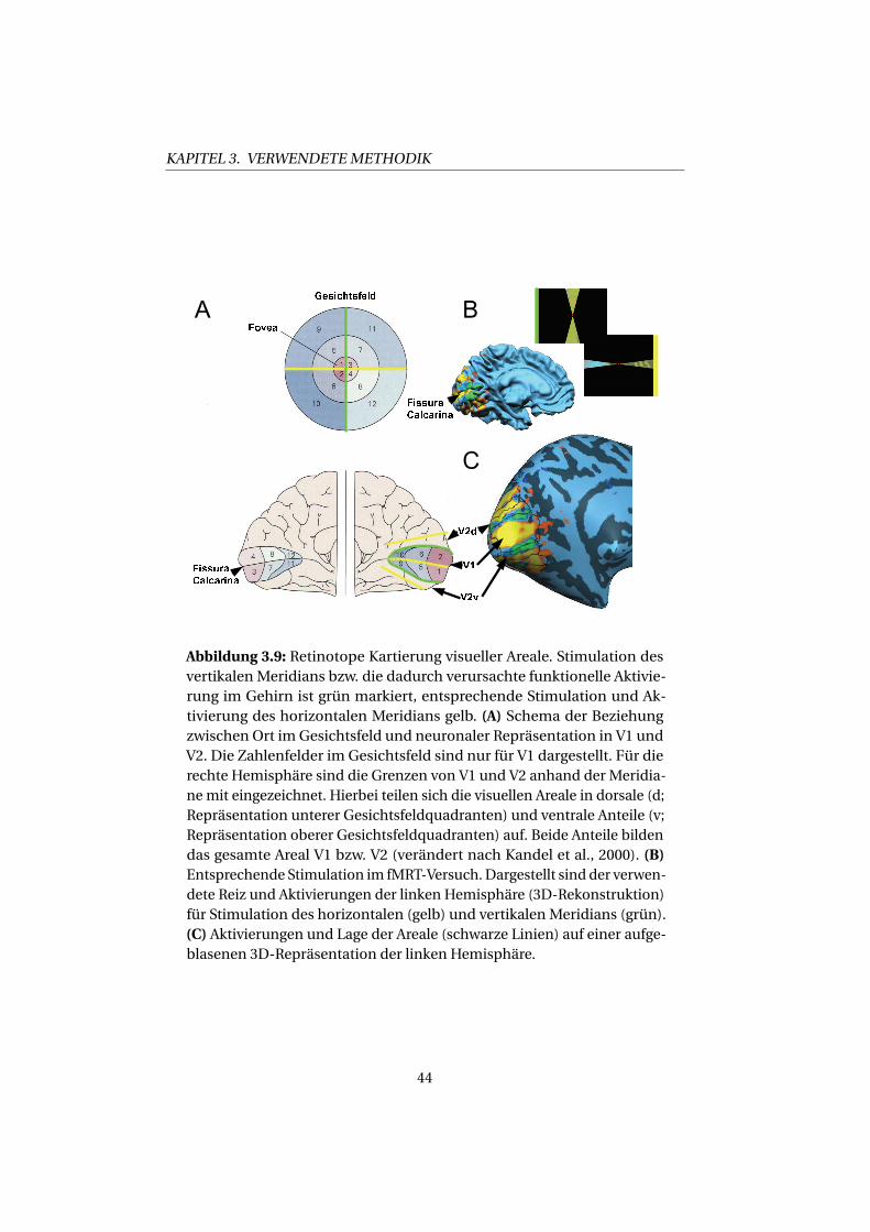
KAPITEL 3. VERWENDETE METHODIK
Abbildung 3.9: Retinotope Kartierung visueller Areale. Stimulation desvertikalen Meridians bzw. die dadurch verursachte funktionelle Aktivie-rung im Gehirn ist grün markiert, entsprechende Stimulation und Ak-tivierung des horizontalen Meridians gelb. (A) Schema der Beziehungzwischen Ort im Gesichtsfeld und neuronaler Repräsentation in V1 undV2. Die Zahlenfelder im Gesichtsfeld sind nur für V1 dargestellt. Für dierechte Hemisphäre sind die Grenzen von V1 und V2 anhand der Meridia-ne mit eingezeichnet. Hierbei teilen sich die visuellen Areale in dorsale (d;Repräsentation unterer Gesichtsfeldquadranten) und ventrale Anteile (v;Repräsentation oberer Gesichtsfeldquadranten) auf. Beide Anteile bildendas gesamte Areal V1 bzw. V2 (verändert nach Kandel et al., 2000). (B)Entsprechende Stimulation im fMRT-Versuch. Dargestellt sind der verwen-dete Reiz und Aktivierungen der linken Hemisphäre (3D-Rekonstruktion)für Stimulation des horizontalen (gelb) und vertikalen Meridians (grün).(C) Aktivierungen und Lage der Areale (schwarze Linien) auf einer aufge-blasenen 3D-Repräsentation der linken Hemisphäre.
44
3.3. FMRT
der Fissura Calcarina bis zur Mitte der Aktivierungen auf dem vertikalen
Meridian. Dann schließt sich V2 an, dessen Grenze bis zur Mitte der Ak-
tivierungen auf den horizontalen Meridian geht, usw. (siehe Abb. 3.9C).
Auf diese Art kann man Grenzen bis in das vierte visuelle Areal finden.
Danach löst sich die retinotope Ordnung immer mehr auf.
Nach erfolgreicher Kartierung kann man nun im Hauptversuch unter-
suchen, inwieweit das BOLD-Signal in den einzelnen visuellen Arealen
entsprechend der jeweiligen Versuchsbedingung verändert ist.
3.3.2 Cortex Based Alignment
Hat man nicht die Möglichkeit, kartierte Gehirne zu verwenden, da
nicht klar ist, wo die Effekte lokalisiert sind, so muss man unter Um-
ständen das gesamte Gehirn betrachten. Hierbei hat man das Problem,
dass bereits auf anatomischer Ebene individuelle Unterschiede existie-
ren. Eine Möglichkeit, damit umzugehen, liefert das „Cortex Based Ali-
gnment” (übersetzt: Angleichung basierend auf dem Kortex). Das Cor-
tex Based Alignment reduziert individuelle Unterschiede, indem 3D-
Rekonstruktionen der untersuchten Gehirne einer Studie ineinander
überführt werden (Goebel et al., 2006). Dabei werden beide Hemisphären
getrennt behandelt. Das Verfahren basiert rein auf der Anatomie und
ist daher dazu geeignet, anatomische Unterschiede zu kompensieren;
individuelle Unterschiede in der Lage funktioneller Areale werden nicht
berücksichtigt. Das Cortex Based Alignment wurde in der fMRT-Studie
dieser Arbeit (Kapitel 7) verwendet, umUnterschiede außerhalb der kar-
tierten visuellen Areale zu finden.
Das Prinzip des Cortex Based Alignments ist in Abb. 3.10 dargestellt.
Die eigentliche Angleichung benutzt eine Kugel-Repräsentation der He-
misphäre, welche bereits eine Standardisierung darstellt, da individuelle
Größenunterschiede herausfallen (die Kugel hat eine definierte Größe).
Anhand der Lage der Gyri (Windungen) und Sulci (Furchen) gleicht das
Verfahren die individuellen Gehirne aneinander an. Das Ergebnis ist eine
Durchschnittsrepräsentation der Hemisphäre über alle Versuchsperso-
nen einer Studie. Die funktionellen Daten werden ebenfalls in das so
45
KAPITEL 3. VERWENDETE METHODIK
$ �
�
Abbildung 3.10: Cortex Based Alignment. (A) Für jede Hemisphäre je-der Versuchsperson wird eine 3D-Rekonstruktion erstellt. (B)Diese 3D-Rekonstruktion wird in eine Kugel transformiert, auf deren Basis alleHemisphären (links und rechts getrennt) aneinander angeglichen wer-den. Gyri sind in gelb dargestellt, Sulci in blau. (C) Die funktionelle Datenwerden ebenfalls transformiert und können nun auf dem angeglichenenGehirn der Gruppe analysiert werden.
gewonnene Gruppengehirn überführt und anschließend analysiert, z.B.
mit dem ALM (siehe Abschnitt 3.3).
46

Kapitel 4
Zusammenfassung & Fazit
Die vorliegende Arbeit beschäftigt sich mit den psychophysikalischen
und neuronalen Eigenschaften der Figur-Grund-Unterscheidung i) bei
unterschiedlicher Zusammensetzung der zur Wahrnehmung der Figur
führendenMerkmale und ii) unter verschiedenen Aufgabenstellungen
(Detektion und Identifikation). Die EEG-Studien behandeln Veränderun-
gen der Figur-Salienz in Abhängigkeit zu den verwendetenMerkmalen.
Dies wurde getrennt für Detektion (Kapitel 5) und Identifikation (Kapitel
6) untersucht. Mit Hilfe der funktionellen Bildgebung wurden schließ-
lich die neuronalen Korrelate der Detektion und Identifikation direkt
verglichen (Kapitel 7).
4.1 Fragestellung undMotivation
Wir sehen Objekte immer als Ganzes, unsere Wahrnehmung basiert je-
doch oft auf Unterschieden bezüglich mehrerer Merkmale (z.B. Tiefe,
Helligkeit oder Farbe), die unterschiedlich stark ausgeprägt sein können.
Bis heute ist weitgehend unklar, inwieweit spezifische Merkmale bei der
Objektverarbeitung interagieren, da psychophysikalische Studien unter-
schiedliche Resultate erhielten, die von den verwendeten Merkmalen
und der Art der Aufgabe abhingen. In den Studien dieser Arbeit wurde
die Salienz der Figur benutzt um i) unterschiedliche Figur-Merkmale und
deren Kombination miteinander zu vergleichen und ii) Detektion und
47
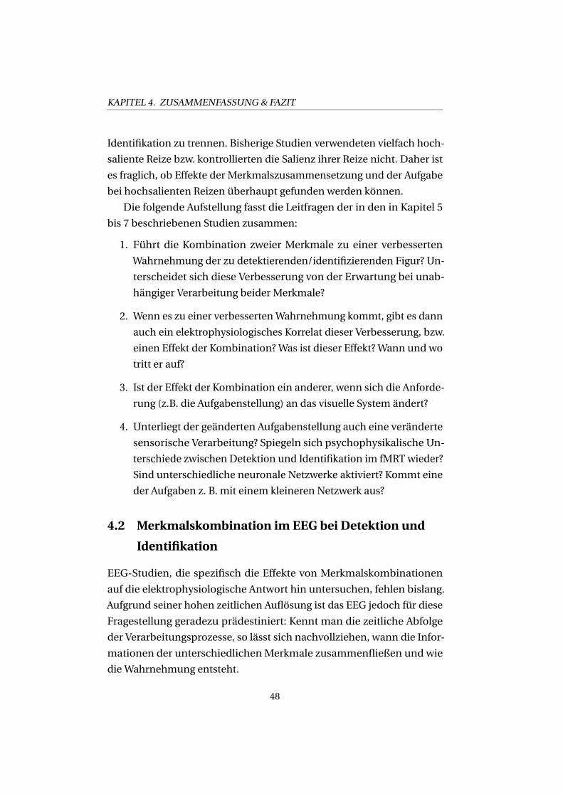
KAPITEL 4. ZUSAMMENFASSUNG & FAZIT
Identifikation zu trennen. Bisherige Studien verwendeten vielfach hoch-
saliente Reize bzw. kontrollierten die Salienz ihrer Reize nicht. Daher ist
es fraglich, ob Effekte der Merkmalszusammensetzung und der Aufgabe
bei hochsalienten Reizen überhaupt gefunden werden können.
Die folgende Aufstellung fasst die Leitfragen der in den in Kapitel 5
bis 7 beschriebenen Studien zusammen:
1. Führt die Kombination zweier Merkmale zu einer verbesserten
Wahrnehmung der zu detektierenden/identifizierenden Figur? Un-
terscheidet sich diese Verbesserung von der Erwartung bei unab-
hängiger Verarbeitung beider Merkmale?
2. Wenn es zu einer verbesserten Wahrnehmung kommt, gibt es dann
auch ein elektrophysiologisches Korrelat dieser Verbesserung, bzw.
einen Effekt der Kombination? Was ist dieser Effekt? Wann und wo
tritt er auf?
3. Ist der Effekt der Kombination ein anderer, wenn sich die Anforde-
rung (z.B. die Aufgabenstellung) an das visuelle System ändert?
4. Unterliegt der geänderten Aufgabenstellung auch eine veränderte
sensorische Verarbeitung? Spiegeln sich psychophysikalische Un-
terschiede zwischen Detektion und Identifikation im fMRT wieder?
Sind unterschiedliche neuronale Netzwerke aktiviert? Kommt eine
der Aufgaben z. B. mit einem kleineren Netzwerk aus?
4.2 Merkmalskombination im EEG bei Detektion und
Identifikation
EEG-Studien, die spezifisch die Effekte von Merkmalskombinationen
auf die elektrophysiologische Antwort hin untersuchen, fehlen bislang.
Aufgrund seiner hohen zeitlichen Auflösung ist das EEG jedoch für diese
Fragestellung geradezu prädestiniert: Kennt man die zeitliche Abfolge
der Verarbeitungsprozesse, so lässt sich nachvollziehen, wann die Infor-
mationen der unterschiedlichenMerkmale zusammenfließen und wie
die Wahrnehmung entsteht.
48
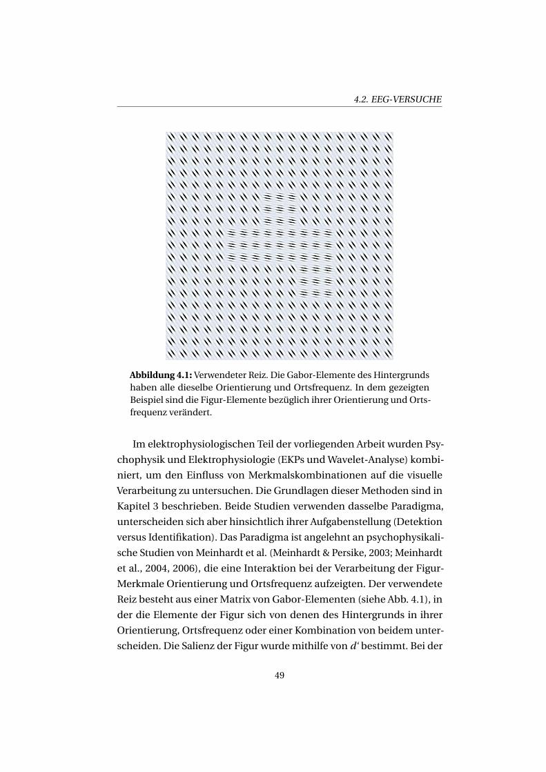
4.2. EEG-VERSUCHE
Abbildung 4.1: Verwendeter Reiz. Die Gabor-Elemente des Hintergrundshaben alle dieselbe Orientierung und Ortsfrequenz. In dem gezeigtenBeispiel sind die Figur-Elemente bezüglich ihrer Orientierung und Orts-frequenz verändert.
Im elektrophysiologischen Teil der vorliegenden Arbeit wurden Psy-
chophysik und Elektrophysiologie (EKPs undWavelet-Analyse) kombi-
niert, um den Einfluss von Merkmalskombinationen auf die visuelle
Verarbeitung zu untersuchen. Die Grundlagen dieser Methoden sind in
Kapitel 3 beschrieben. Beide Studien verwenden dasselbe Paradigma,
unterscheiden sich aber hinsichtlich ihrer Aufgabenstellung (Detektion
versus Identifikation). Das Paradigma ist angelehnt an psychophysikali-
sche Studien vonMeinhardt et al. (Meinhardt & Persike, 2003; Meinhardt
et al., 2004, 2006), die eine Interaktion bei der Verarbeitung der Figur-
Merkmale Orientierung und Ortsfrequenz aufzeigten. Der verwendete
Reiz besteht aus einer Matrix von Gabor-Elementen (siehe Abb. 4.1), in
der die Elemente der Figur sich von denen des Hintergrunds in ihrer
Orientierung, Ortsfrequenz oder einer Kombination von beidem unter-
scheiden. Die Salienz der Figur wurdemithilfe von d‘ bestimmt. Bei der
49
KAPITEL 4. ZUSAMMENFASSUNG & FAZIT
Detektionsstudie beantworteten die Versuchspersonen in einer 2-AFC,
ob sie die Figur links oder rechts des Fixationspunktes gesehen hatten.
Hierbei war es nicht zwingend notwendig, die ganze Figur zu erkennen.
Bei der Identifikationsstudie mussten die Probanden hingegen zwischen
Bild und Spiegelbild der Figur unterscheiden und somit genau wiederge-
ben,was sie gesehen hatten.
Beide Studien konnten psychophysikalisch die Ergebnisse vonMein-
hardt et al. bestätigen. Orientierung und Ortsfrequenz interagieren als
Figur-Merkmale, so dass ihre Kombination die Salienz deutlich erhöht.
In der Elektrophysiologie zeigt sich, dass die frühesten Effekte mit der Sa-
lienz (d‘) korrelieren. Dies drückt sich in einer sinkenden Amplitude der
posterioren P2-Komponente mit steigender Salienz aus, was zusätzlich
durch eine Reduktion im θ-Frequenzband nachgewiesen werden konnte.
Dieser Befund deutet darauf hin, dass der durch das Zusammenspiel der
Merkmalewahrgenommene Figur-Grund-Unterschied (die Salienz) die
neuronale Antwort viel direkter prägt als der physikalische Figur-Grund-
Unterschied an sich: Der gefundene Amplituden-Effekt der P2 erwies
sich in der Tat als sensitiv für die Salienz der Figur, nicht aber als ebenso
sensitiv für ihre physikalischen Eigenschaften (beispielsweise ob sie nur
ein Merkmal oder zwei beinhaltete).
Dieses Ergebnis wurde in beiden Studien, d.h. für Detektion und Iden-
tifikation, gefunden, was die Robustheit der psychophysikalischen und
elektrophysiologischen Ergebnisse über die Aufgabenstellung hinweg
verdeutlicht. Die Identifikation war die schwierigere Aufgabe, d.h. um
zu gleicher Leistung (in Anteilen richtiger Antworten) wie bei der De-
tektion zu kommen, benötigten die Probanden der Identifikationsstudie
einen höheren physikalischen Figur-Grund-Unterschied. Anders gesagt,
bei gleichem d‘ für Detektion und Identifikation gibt es einen physikali-
schen Unterschied der Merkmalsausprägung. Demnach unterscheiden
sich beide Studien in der Aufgabe und den verwendeten Figur-Grund
Unterschieden. Trotzdemwurden qualitativ dieselben Effekte mit einer
vergleichbaren Amplitude der P2-Komponente in beiden Studien ge-
funden. Diese Ergebnisse beider Studien deuten darauf hin, dass der
50
4.3. VERGLEICH VON DETEKTION UND IDENTIFIKATION IM FMRT
gemessene Salienz-Effekt in der elektrophysiologischen Antwort unab-
hängig von der Aufgabe ist. Der physikalische Figur-Grund-Unterschied
(der zu der gemessenen Salienz führt) hängt hingegen immer von der
jeweiligen Aufgabe ab. Diese Idee der aufgabenspezifischen Beziehung
zwischen physikalischem Figur-Grund-Unterschied und Salienz wurde
in der im Folgenden beschriebenen fMRT-Studie benutzt, um die beiden
Aufgaben zu trennen.
4.3 Vergleich von Detektion und Identifikation im fMRT
Bisherige fMRT-Studien zur Trennung von Detektion und Identifikation
berücksichtigten nicht die Salienz ihrer Reize und fanden –eventuell des-
halb– keine Unterschiede zwischen beiden Aufgaben. Bei Figur-Grund-
Unterschieden, die eine Identifikation ermöglichen, kann eine Detektion
immer miterfolgen, da sie die einfachere Aufgabe ist. Umgekehrt aber ist
nicht bei jeder erfolgreichen Detektion auch eine Identifikation möglich.
In der fMRT Studie wurde ein ähnlicher Reiz wie in den beiden EEG-
Studien verwendet (siehe Abb. 4.1), allerdings gab es nur noch ein Merk-
mal für die Figur, nämlich die Orientierung ihrer Elemente.
Die psychophysikalischen Ergebnisse dieser Studie bestätigen die
im Vergleich der EEG-Studien gefundenen Unterschiede der Wahrneh-
mungsschwellen zwischen beiden Aufgaben: Bei vergleichbarer Salienz
lag der benötigte Figur-Grund-Unterschied für die Detektion weit un-
ter dem erforderlichen Unterschied für die Identifikation. Dieser Effekt
wurde von Anfang an gefunden und blieb auch nach Training stabil. Au-
ßerdem zeigten Reaktionszeit-Messungen, dass längere Reaktionszeiten
für die Identifikation benötigt wurden als für die Detektion. Dieses Er-
gebnis legt nahe, dass die Identifikation mehr Zeit benötigt, evtl. sogar
zusätzliche spezialisierte Areale im Gehirn.
Alle kartierten visuellen Areale zeigten während der Detektion und
der Identifikation erhöhte Aktivierung im Vergleich zu einer Ruhebe-
dingung. Statistische Tests zeigten, dass diese Aktivierung sich erst in
spezialisierten, objektsensitiven Arealen für Detektion und Identifika-
tion unterschied, indem diese während der Identifikation ein höheres
51
KAPITEL 4. ZUSAMMENFASSUNG & FAZIT
BOLD-Signal aufwiesen. Diese Unterschiede wurden in zwei Unterein-
heiten (LO und pFs) des Lateralen-Okzipitalen-Komplex (LOC) sowie in
einer benachbarten Region (CoS) im kollateralen Sulcus gefunden. Dieser
Aktivierungsunterschied konnte nicht auf den erhöhten Figur-Grund-
Unterschied bei der Identifikation zurückgeführt werden, da diese Areale
in einer Kontrollbedingung mit gleichem physikalischen Figur-Grund-
Unterschied aber ohne erkennbare Figur ebenfalls schwächer aktiviert
wurden als bei der Identifikation. Zusammenmit der Psychophysik legen
diese Ergebnisse nahe, dass objektsensitive Areale nicht zwingend an der
Detektion beteiligt sind.
4.4 Fazit
Die Salienz einer Figur ist die entscheidende Einheit unserer Wahrneh-
mung. Sie hat ihr elektrophysiologisches Korrelat etwa bei 200ms, da sie
in beiden EEG-Studien die Amplitude der posterioren P2-Komponente
beeinflusste. Salienz entsteht aus dem Zusammenspiel der vorhandenen
Figur-Merkmale, die zumindest teilweise bei der Verarbeitung interagie-
ren, wie für die Merkmale Orientierung und Ortsfrequenz gezeigt wurde.
Es bleibt zu klären, ob die gefundenen Effekte auch für andere Merkmals-
kombinationen bestätigt werden können. Des Weiteren wird die Salienz
nicht nur durch die Physik des Reizes beeinflusst, sondern auch durch die
Relevanz des Gesehenen: Um einem Tier mit dem Auto auszuweichen,
muss ich es nicht unbedingt identifizieren; es reicht aus, wenn ich dort
etwas detektiere.
Die Psychophysik zeigt in allen drei Studien, dass Detektion und
Identifikation verschiedene Charakteristika haben. Die Detektion ist der
schnellere Prozess, und man kann sie bereits erfolgreich durchführen,
wennmandie ganze Figur noch gar nicht erkennt. Die fMRT-Daten zeigen
zudem übereinstimmend, dass objektsensitive Areale stärker während
der Identifikation angeregt werden als nur durch die Detektion. Offen
bleibt die Frage, ob beide Aufgaben von z.T. unterschiedlichen neuro-
nalen Verarbeitungspfaden gelöst werden, was in der fMRT-Studie nicht
eindeutig zu zeigen war. Beispielsweise bleibt es zu klären, ob Areale im
52

4.4. FAZIT
LOC wirklich für eine Detektion notwendig sind, oder ob die gefundene
Aktivierung von LOC während der Detektion lediglich bedeutet, dass das
Gehirn versucht hat, etwas zu identifizieren.
53

Kapitel 5
The electrophysiological
correlate of saliency: evidence
from a figure-detection task
Sirko Straube &Manfred Fahle
Abstract
Although figure-ground segregation in a natural environment usually
relies on multiple cues, we experience a coherent figure without usu-
ally noticing the individual single cues. It is still unclear how various
cues interact to achieve this unified percept and whether this interaction
depends on task demands. Studies investigating the effect of cue com-
bination on the human EEG are still lacking. In the present study, we
combined psychophysics, ERP and time-frequency analysis to investigate
the interaction of orientation and spatial frequency as visual cues in a
figure detection task. The figure was embedded in a matrix of Gabor
elements, and we systematically varied figure saliency by changing the
underlying cue configuration. We found a strong correlation between the
posterior P2 amplitude and the perceived saliency of the figure: The P2
55
KAPITEL 5. SALIENCY-ERP & DETECTION TASK
amplitude decreased with increasing saliency. Analogously, the power
of the θ-band decreased for more salient figures. At longer latencies,
the posterior P3 component was modulated in amplitude and latency,
possibly reflecting increased decision confidence at higher saliencies.
In conclusion, when the cue composition (e.g. one or two cues) or cue
strength is changed in a figure detection task, first differences in the elec-
trophysiological response reflect the perceived saliency and not directly
the underlying cue configuration.
5.1 Introduction
The first cue for object presence in a visual scene is the local difference of
a visual feature (e.g. a difference in colour, luminance, depth or motion).
The detection of such basic differences at a glance is a powerful tool
to rapidly evaluate which locations might contain objects and to start
preparing appropriate actions. Accordingly, it has been suggested that
a large amount of attention is caught by such bottom-up, image-based
saliency cues (for reviews see e.g. Itti & Koch, 2001; Treue, 2003). But how
is the saliency formed when figure-ground segregation can rely onmulti-
ple cues? Is the processing of these cues independent or do cues interact?
The answers to these questions seem to depend both on task and on cue
type: The majority of studies observe cue interaction (Kubovy et al., 1999;
Kubovy & Cohen, 2001; Meinhardt & Persike, 2003; Meinhardt et al., 2004,
2006; van Mierlo et al., 2007; Nothdurft, 2000; Persike & Meinhardt, 2006;
Rivest & Cavanagh, 1996), while others report independent processing
(Leonards & Singer, 2000; Pashler, 1988; Phillips & Craven, 2000; Phillips,
2001; Treisman & Gelade, 1980; Tsujimoto & Tayama, 2004). Additionally,
there is growing evidence that the effects caused by combination of visual
cuesmight not be the outcome of a hard-wired system, but rather that of a
dynamic system allowing for optimal combination depending on the reli-
ability of the cues and the nature of the task (Blake et al., 1993; Hillis et al.,
2004; Jacobs & Fine, 1999; Landy & Kojima, 2001; Oruc et al., 2003; Triesch
et al., 2002). The neuronal mechanisms underlying these behavioural
findings in humans are unclear, and the effect of cue combination on the
56
5.1. INTRODUCTION
human electroencephalogram (EEG) remains unexplored, although the
high temporal resolution of the EEGmight indicate if and when neural
responses reflect primarily the physical figure-ground properties or the
perceived saliency. Combined with behavioural measurements on cue
combination (providing evidence that cue interaction occurred), such
data could provide insights on where and when the coherent percept is
formed. Existing electrophysiological studies mainly concentrated on
the general effect of textures or figures on the EEG. They found that tex-
tures induce a texture-segregation visual evoked potential (tsVEP) with a
latency between 100 ms and 300 ms (Bach &Meigen, 1992, 1997; Bach
et al., 2000; Caputo & Casco, 1999; Fahle et al., 2003; Lamme et al., 1992).
The tsVEP is mostly a negative shift of the ‘low-level VEP’ that is similar
for a variety of cues (Bach & Meigen, 1997; Fahle et al., 2003). It shows
an early segregation component affected by the presence of low-level
differences between segregated and homogeneous patterns while not by
task-demands or attention, and a later component modulated by both
attention and task (Heinrich et al., 2007). Other studies, decomposing the
electrophysiological signal into specific frequency bands and investigat-
ing propagation of activity in these bands over time, found segregation-
specific activations in the γ-band (Eckhorn et al., 1988). In the EEG, an
early evoked activation was modulated by stimulus properties (such as
size or eccentricity) in object detection and discrimination (Busch et al.,
2004, 2006; Senkowski & Herrmann, 2002) while a late induced activation
was related to object representation (Tallon-Baudry & Bertrand, 1999).
Taken together, a common characteristic of the electrophysiological
response in both, ERP and time-frequency analysis, is an early segregation-
specific effect (around 100 ms), which is modulated by stimulus-driven,
object-based properties, and a later effect (around 200-250 ms), which is
influenced by perceptual, attentional and/or task-related factors. How-
ever, it remains unclear in what way these correlates of figure-ground
segregation are influenced by cue combination. All the effects reported
may reflect the stimulus changes caused by cue combination, since both
the physical figure-ground properties and the perceived saliency are
57
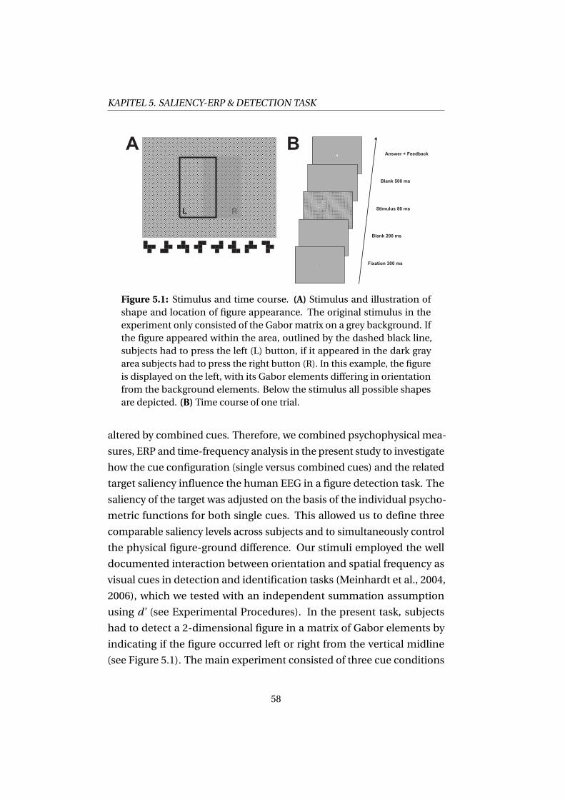
KAPITEL 5. SALIENCY-ERP & DETECTION TASK
L R
A B
Fixation 300 ms
Blank 200 ms
Stimulus 80 ms
Blank 500 ms
Answer + Feedback
Figure 5.1: Stimulus and time course. (A) Stimulus and illustration ofshape and location of figure appearance. The original stimulus in theexperiment only consisted of the Gabor matrix on a grey background. Ifthe figure appeared within the area, outlined by the dashed black line,subjects had to press the left (L) button, if it appeared in the dark grayarea subjects had to press the right button (R). In this example, the figureis displayed on the left, with its Gabor elements differing in orientationfrom the background elements. Below the stimulus all possible shapesare depicted. (B) Time course of one trial.
altered by combined cues. Therefore, we combined psychophysical mea-
sures, ERP and time-frequency analysis in the present study to investigate
how the cue configuration (single versus combined cues) and the related
target saliency influence the human EEG in a figure detection task. The
saliency of the target was adjusted on the basis of the individual psycho-
metric functions for both single cues. This allowed us to define three
comparable saliency levels across subjects and to simultaneously control
the physical figure-ground difference. Our stimuli employed the well
documented interaction between orientation and spatial frequency as
visual cues in detection and identification tasks (Meinhardt et al., 2004,
2006), which we tested with an independent summation assumption
using d’ (see Experimental Procedures). In the present task, subjects
had to detect a 2-dimensional figure in a matrix of Gabor elements by
indicating if the figure occurred left or right from the vertical midline
(see Figure 5.1). The main experiment consisted of three cue conditions
58
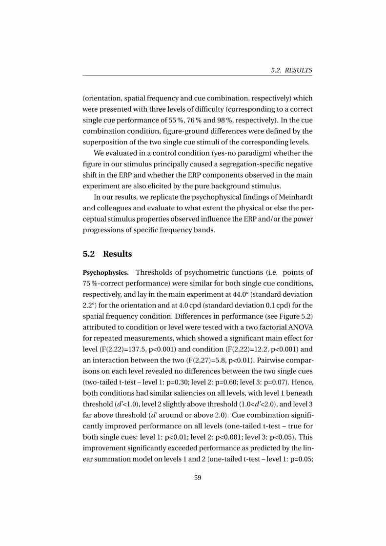
5.2. RESULTS
(orientation, spatial frequency and cue combination, respectively) which
were presented with three levels of difficulty (corresponding to a correct
single cue performance of 55%, 76% and 98%, respectively). In the cue
combination condition, figure-ground differences were defined by the
superposition of the two single cue stimuli of the corresponding levels.
We evaluated in a control condition (yes-no paradigm) whether the
figure in our stimulus principally caused a segregation-specific negative
shift in the ERP and whether the ERP components observed in the main
experiment are also elicited by the pure background stimulus.
In our results, we replicate the psychophysical findings of Meinhardt
and colleagues and evaluate to what extent the physical or else the per-
ceptual stimulus properties observed influence the ERP and/or the power
progressions of specific frequency bands.
5.2 Results
Psychophysics. Thresholds of psychometric functions (i.e. points of
75%-correct performance) were similar for both single cue conditions,
respectively, and lay in the main experiment at 44.0° (standard deviation
2.2°) for the orientation and at 4.0 cpd (standard deviation 0.1 cpd) for the
spatial frequency condition. Differences in performance (see Figure 5.2)
attributed to condition or level were tested with a two factorial ANOVA
for repeatedmeasurements, which showed a significant main effect for
level (F(2,22)=137.5, p<0.001) and condition (F(2,22)=12.2, p<0.001) and
an interaction between the two (F(2,27)=5.8, p<0.01). Pairwise compar-
isons on each level revealed no differences between the two single cues
(two-tailed t-test – level 1: p=0.30; level 2: p=0.60; level 3: p=0.07). Hence,
both conditions had similar saliencies on all levels, with level 1 beneath
threshold (d’<1.0), level 2 slightly above threshold (1.0<d’<2.0), and level 3
far above threshold (d’ around or above 2.0). Cue combination signifi-
cantly improved performance on all levels (one-tailed t-test – true for
both single cues: level 1: p<0.01; level 2: p<0.001; level 3: p<0.05). This
improvement significantly exceeded performance as predicted by the lin-
ear summationmodel on levels 1 and 2 (one-tailed t-test – level 1: p=0.05;
59
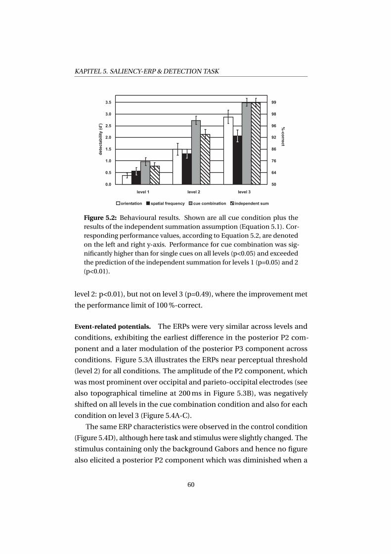
KAPITEL 5. SALIENCY-ERP & DETECTION TASK
0.0
0.5
1.0
1.5
2.0
2.5
3.0
3.5
level 1 level 2 level 3
orientation spatial frequency cue combination independent sum
de
tec
tab
ilit
y(d
’) %-c
orre
ct
50
64
76
86
92
96
98
99
Figure 5.2: Behavioural results. Shown are all cue condition plus theresults of the independent summation assumption (Equation 5.1). Cor-responding performance values, according to Equation 5.2, are denotedon the left and right y-axis. Performance for cue combination was sig-nificantly higher than for single cues on all levels (p<0.05) and exceededthe prediction of the independent summation for levels 1 (p=0.05) and 2(p<0.01).
level 2: p<0.01), but not on level 3 (p=0.49), where the improvement met
the performance limit of 100%-correct.
Event-related potentials. The ERPs were very similar across levels and
conditions, exhibiting the earliest difference in the posterior P2 com-
ponent and a later modulation of the posterior P3 component across
conditions. Figure 5.3A illustrates the ERPs near perceptual threshold
(level 2) for all conditions. The amplitude of the P2 component, which
was most prominent over occipital and parieto-occipital electrodes (see
also topographical timeline at 200ms in Figure 5.3B), was negatively
shifted on all levels in the cue combination condition and also for each
condition on level 3 (Figure 5.4A-C).
The same ERP characteristics were observed in the control condition
(Figure 5.4D), although here task and stimulus were slightly changed. The
stimulus containing only the background Gabors and hence no figure
also elicited a posterior P2 component which was diminished when a
60
5.2. RESULTS
Figure 5.3: Grand-average ERPs (n=12) and topographical timeline atlevel 2. (A) ERPs of the main experiment at all electrodes recorded. Blackarrows denote P2 and P3 component and black underlined electrodenamesmark ROI used for their analysis. (B) Voltage maps (top and backview of the head) of orientation condition at level 2, plotted in intervals of50ms.
61
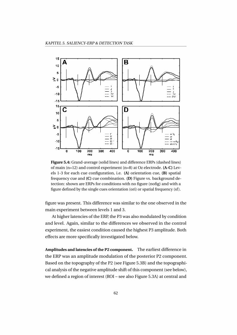
KAPITEL 5. SALIENCY-ERP & DETECTION TASK
Figure 5.4: Grand-average (solid lines) and difference ERPs (dashed lines)of main (n=12) and control experiment (n=8) at Oz electrode. (A-C) Lev-els 1-3 for each cue configuration, i.e. (A) orientation cue, (B) spatialfrequency cue and (C) cue combination. (D) Figure vs. background de-tection: shown are ERPs for conditions with no figure (nofig) and with afigure defined by the single cues orientation (ori) or spatial frequency (sf).
figure was present. This difference was similar to the one observed in the
main experiment between levels 1 and 3.
At higher latencies of the ERP, the P3 was alsomodulated by condition
and level. Again, similar to the differences we observed in the control
experiment, the easiest condition caused the highest P3 amplitude. Both
effects are more specifically investigated below.
Amplitudes and latencies of the P2 component. The earliest difference in
the ERP was an amplitude modulation of the posterior P2 component.
Based on the topography of the P2 (see Figure 5.3B) and the topographi-
cal analysis of the negative amplitude shift of this component (see below),
we defined a region of interest (ROI – see also Figure 5.3A) at central and
62
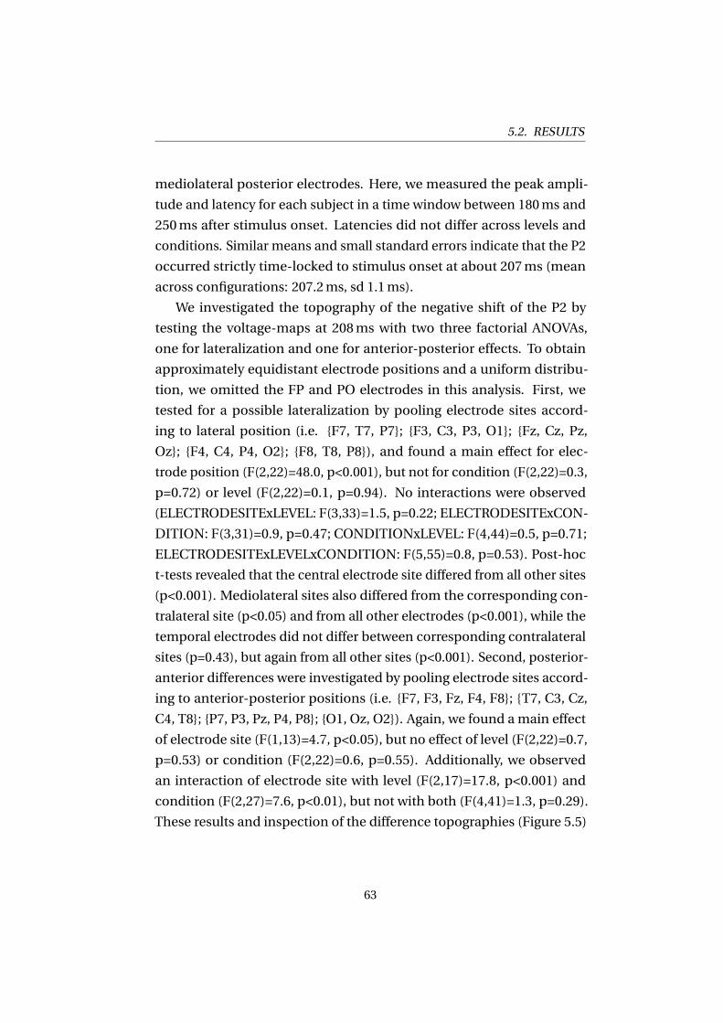
5.2. RESULTS
mediolateral posterior electrodes. Here, we measured the peak ampli-
tude and latency for each subject in a time window between 180ms and
250ms after stimulus onset. Latencies did not differ across levels and
conditions. Similar means and small standard errors indicate that the P2
occurred strictly time-locked to stimulus onset at about 207ms (mean
across configurations: 207.2ms, sd 1.1ms).
We investigated the topography of the negative shift of the P2 by
testing the voltage-maps at 208ms with two three factorial ANOVAs,
one for lateralization and one for anterior-posterior effects. To obtain
approximately equidistant electrode positions and a uniform distribu-
tion, we omitted the FP and PO electrodes in this analysis. First, we
tested for a possible lateralization by pooling electrode sites accord-
ing to lateral position (i.e. {F7, T7, P7}; {F3, C3, P3, O1}; {Fz, Cz, Pz,
Oz}; {F4, C4, P4, O2}; {F8, T8, P8}), and found a main effect for elec-
trode position (F(2,22)=48.0, p<0.001), but not for condition (F(2,22)=0.3,
p=0.72) or level (F(2,22)=0.1, p=0.94). No interactions were observed
(ELECTRODESITExLEVEL: F(3,33)=1.5, p=0.22; ELECTRODESITExCON-
DITION: F(3,31)=0.9, p=0.47; CONDITIONxLEVEL: F(4,44)=0.5, p=0.71;
ELECTRODESITExLEVELxCONDITION: F(5,55)=0.8, p=0.53). Post-hoc
t-tests revealed that the central electrode site differed from all other sites
(p<0.001). Mediolateral sites also differed from the corresponding con-
tralateral site (p<0.05) and from all other electrodes (p<0.001), while the
temporal electrodes did not differ between corresponding contralateral
sites (p=0.43), but again from all other sites (p<0.001). Second, posterior-
anterior differences were investigated by pooling electrode sites accord-
ing to anterior-posterior positions (i.e. {F7, F3, Fz, F4, F8}; {T7, C3, Cz,
C4, T8}; {P7, P3, Pz, P4, P8}; {O1, Oz, O2}). Again, we found amain effect
of electrode site (F(1,13)=4.7, p<0.05), but no effect of level (F(2,22)=0.7,
p=0.53) or condition (F(2,22)=0.6, p=0.55). Additionally, we observed
an interaction of electrode site with level (F(2,17)=17.8, p<0.001) and
condition (F(2,27)=7.6, p<0.01), but not with both (F(4,41)=1.3, p=0.29).
These results and inspection of the difference topographies (Figure 5.5)
63
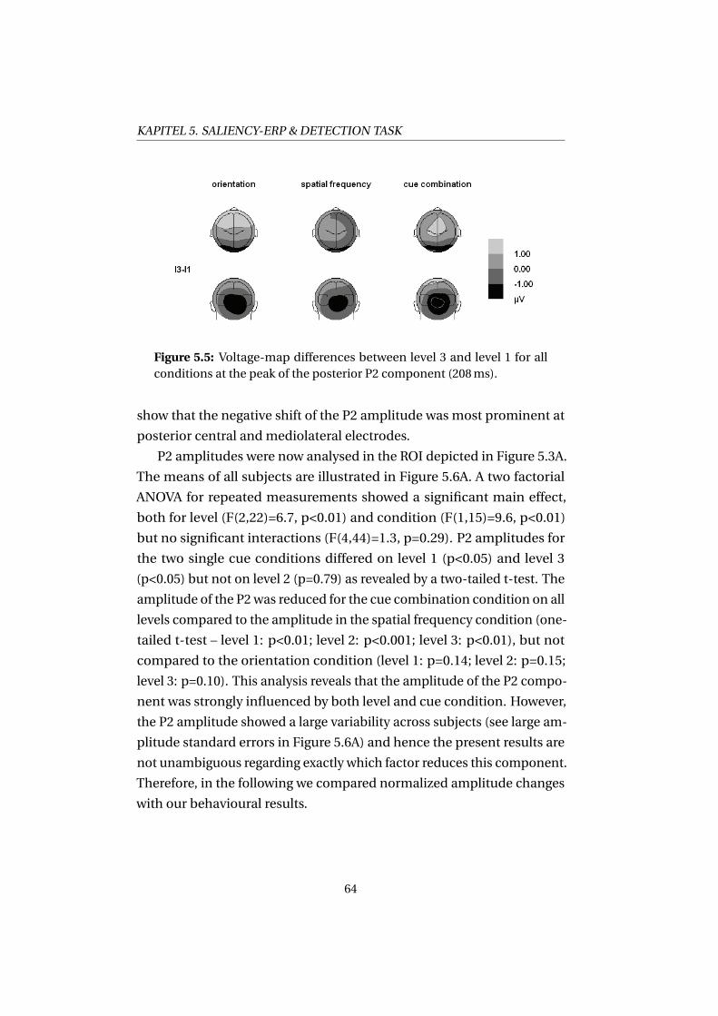
KAPITEL 5. SALIENCY-ERP & DETECTION TASK
Figure 5.5: Voltage-map differences between level 3 and level 1 for allconditions at the peak of the posterior P2 component (208ms).
show that the negative shift of the P2 amplitude was most prominent at
posterior central and mediolateral electrodes.
P2 amplitudes were now analysed in the ROI depicted in Figure 5.3A.
The means of all subjects are illustrated in Figure 5.6A. A two factorial
ANOVA for repeated measurements showed a significant main effect,
both for level (F(2,22)=6.7, p<0.01) and condition (F(1,15)=9.6, p<0.01)
but no significant interactions (F(4,44)=1.3, p=0.29). P2 amplitudes for
the two single cue conditions differed on level 1 (p<0.05) and level 3
(p<0.05) but not on level 2 (p=0.79) as revealed by a two-tailed t-test. The
amplitude of the P2 was reduced for the cue combination condition on all
levels compared to the amplitude in the spatial frequency condition (one-
tailed t-test – level 1: p<0.01; level 2: p<0.001; level 3: p<0.01), but not
compared to the orientation condition (level 1: p=0.14; level 2: p=0.15;
level 3: p=0.10). This analysis reveals that the amplitude of the P2 compo-
nent was strongly influenced by both level and cue condition. However,
the P2 amplitude showed a large variability across subjects (see large am-
plitude standard errors in Figure 5.6A) and hence the present results are
not unambiguous regarding exactly which factor reduces this component.
Therefore, in the following we compared normalized amplitude changes
with our behavioural results.
64
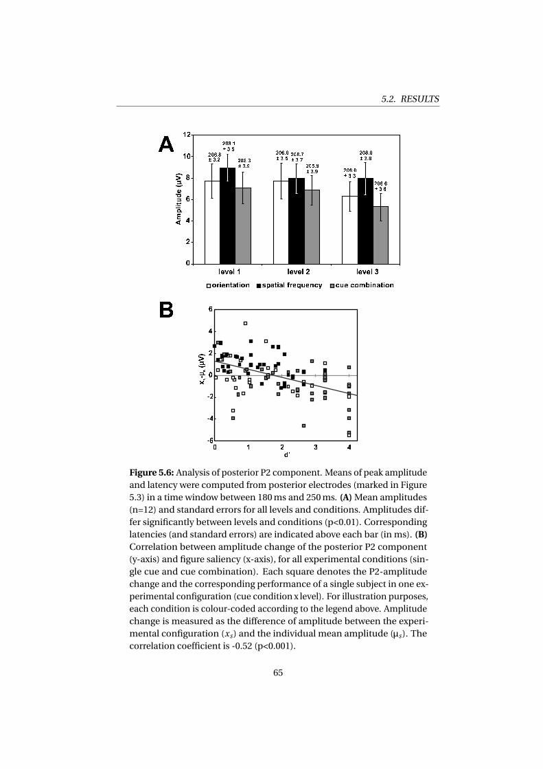
5.2. RESULTS
Figure 5.6: Analysis of posterior P2 component. Means of peak amplitudeand latency were computed from posterior electrodes (marked in Figure5.3) in a time window between 180ms and 250ms. (A)Mean amplitudes(n=12) and standard errors for all levels and conditions. Amplitudes dif-fer significantly between levels and conditions (p<0.01). Correspondinglatencies (and standard errors) are indicated above each bar (in ms). (B)Correlation between amplitude change of the posterior P2 component(y-axis) and figure saliency (x-axis), for all experimental conditions (sin-gle cue and cue combination). Each square denotes the P2-amplitudechange and the corresponding performance of a single subject in one ex-perimental configuration (cue condition x level). For illustration purposes,each condition is colour-coded according to the legend above. Amplitudechange is measured as the difference of amplitude between the experi-mental configuration (xs) and the individual mean amplitude (μs). Thecorrelation coefficient is -0.52 (p<0.001).
65
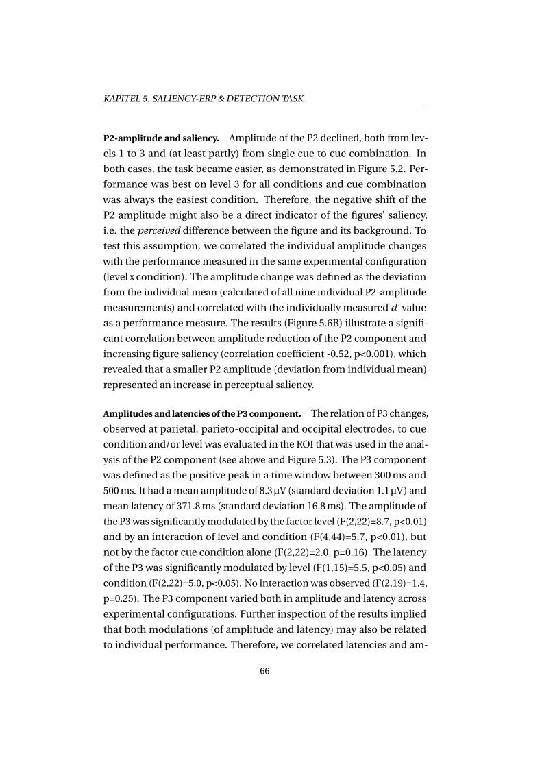
KAPITEL 5. SALIENCY-ERP & DETECTION TASK
P2-amplitude and saliency. Amplitude of the P2 declined, both from lev-
els 1 to 3 and (at least partly) from single cue to cue combination. In
both cases, the task became easier, as demonstrated in Figure 5.2. Per-
formance was best on level 3 for all conditions and cue combination
was always the easiest condition. Therefore, the negative shift of the
P2 amplitude might also be a direct indicator of the figures’ saliency,
i.e. the perceived difference between the figure and its background. To
test this assumption, we correlated the individual amplitude changes
with the performance measured in the same experimental configuration
(level x condition). The amplitude change was defined as the deviation
from the individual mean (calculated of all nine individual P2-amplitude
measurements) and correlated with the individually measured d’ value
as a performance measure. The results (Figure 5.6B) illustrate a signifi-
cant correlation between amplitude reduction of the P2 component and
increasing figure saliency (correlation coefficient -0.52, p<0.001), which
revealed that a smaller P2 amplitude (deviation from individual mean)
represented an increase in perceptual saliency.
Amplitudes and latencies of theP3component. The relation of P3 changes,
observed at parietal, parieto-occipital and occipital electrodes, to cue
condition and/or level was evaluated in the ROI that was used in the anal-
ysis of the P2 component (see above and Figure 5.3). The P3 component
was defined as the positive peak in a time window between 300ms and
500ms. It had amean amplitude of 8.3μV (standard deviation 1.1μV) and
mean latency of 371.8ms (standard deviation 16.8ms). The amplitude of
the P3was significantlymodulated by the factor level (F(2,22)=8.7, p<0.01)
and by an interaction of level and condition (F(4,44)=5.7, p<0.01), but
not by the factor cue condition alone (F(2,22)=2.0, p=0.16). The latency
of the P3 was significantly modulated by level (F(1,15)=5.5, p<0.05) and
condition (F(2,22)=5.0, p<0.05). No interactionwas observed (F(2,19)=1.4,
p=0.25). The P3 component varied both in amplitude and latency across
experimental configurations. Further inspection of the results implied
that both modulations (of amplitude and latency) may also be related
to individual performance. Therefore, we correlated latencies and am-
66
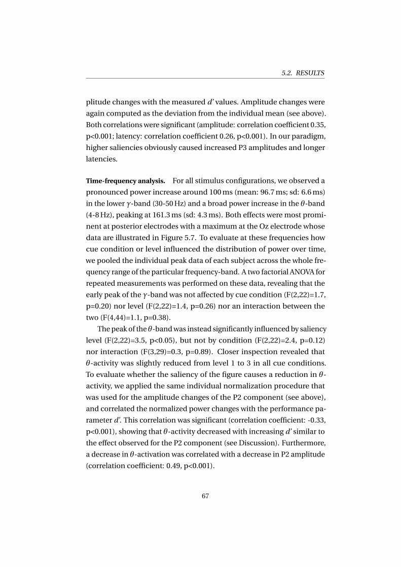
5.2. RESULTS
plitude changes with the measured d’ values. Amplitude changes were
again computed as the deviation from the individual mean (see above).
Both correlationswere significant (amplitude: correlation coefficient 0.35,
p<0.001; latency: correlation coefficient 0.26, p<0.001). In our paradigm,
higher saliencies obviously caused increased P3 amplitudes and longer
latencies.
Time-frequency analysis. For all stimulus configurations, we observed a
pronounced power increase around 100ms (mean: 96.7ms; sd: 6.6ms)
in the lower γ-band (30-50Hz) and a broad power increase in the θ-band
(4-8Hz), peaking at 161.3ms (sd: 4.3ms). Both effects were most promi-
nent at posterior electrodes with a maximum at the Oz electrode whose
data are illustrated in Figure 5.7. To evaluate at these frequencies how
cue condition or level influenced the distribution of power over time,
we pooled the individual peak data of each subject across the whole fre-
quency range of the particular frequency-band. A two factorial ANOVA for
repeated measurements was performed on these data, revealing that the
early peak of the γ-band was not affected by cue condition (F(2,22)=1.7,
p=0.20) nor level (F(2,22)=1.4, p=0.26) nor an interaction between the
two (F(4,44)=1.1, p=0.38).
The peak of the θ-bandwas instead significantly influencedby saliency
level (F(2,22)=3.5, p<0.05), but not by condition (F(2,22)=2.4, p=0.12)
nor interaction (F(3,29)=0.3, p=0.89). Closer inspection revealed that
θ-activity was slightly reduced from level 1 to 3 in all cue conditions.
To evaluate whether the saliency of the figure causes a reduction in θ-
activity, we applied the same individual normalization procedure that
was used for the amplitude changes of the P2 component (see above),
and correlated the normalized power changes with the performance pa-
rameter d’. This correlation was significant (correlation coefficient: -0.33,
p<0.001), showing that θ-activity decreased with increasing d’ similar to
the effect observed for the P2 component (see Discussion). Furthermore,
a decrease in θ-activation was correlated with a decrease in P2 amplitude
(correlation coefficient: 0.49, p<0.001).
67
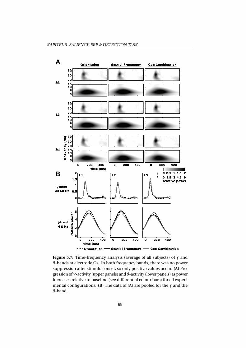
KAPITEL 5. SALIENCY-ERP & DETECTION TASK
Figure 5.7: Time-frequency analysis (average of all subjects) of γ andθ-bands at electrode Oz. In both frequency bands, there was no powersuppression after stimulus onset, so only positive values occur. (A) Pro-gression of γ-activity (upper panels) and θ-activity (lower panels) as powerincreases relative to baseline (see differential colour bars) for all experi-mental configurations. (B) The data of (A) are pooled for the γ and theθ-band.
68
5.3. DISCUSSION
5.3 Discussion
Consistent with previous studies (Meinhardt & Persike, 2003; Meinhardt
et al., 2004, 2006) we observed an interaction between the orientation
and spatial frequency cues during the detection of a figure. This interac-
tion was revealed on all saliency levels by a performance benefit for cue
combination, exceeding the prediction of an independent summation
assumption. In the present study we moreover demonstrated that the
electrophysiological response reflects this performance benefit by means
of an amplitude decrease of the posterior P2 component between 150ms
and 250ms and a corresponding reduction in θ-power, indicating that
neural activity at these latencies is closely related to perception, which is
non-linearly related to the underlying cues. In addition, the posterior P3
component of the ERP increases in amplitude and latency from level 1 to
3 at higher latencies.
The P2-effect and physical stimulus properties. The figure present in the
stimulus as compared to the stimulus without a figure (Figure 5.4D)
causes the well-known segregation-specific negativity in the ERP (Bach
& Meigen, 1992, 1997; Bach et al., 2000; Caputo & Casco, 1999; Fahle
et al., 2003; Heinrich et al., 2007; Mathes et al., 2006; Mathes & Fahle,
2007). This negativity has similar characteristics for both single cues
(Figure 5.4D). Since the figure is always present in the main experiment,
the segregation-specific shift becomes considerably blurred in the ERPs
(see difference ERPs in Figure 5.4A-C). The remaining differences can
either be attributed to the different physical cue configurations or to
different saliencies. The correlation between physical figure-ground
difference and saliency (measured as performance) is given by the psy-
chometric function. The P2 amplitude modulation is clearly related to
figure saliency (Figure 5.6B), but it is not unambiguously clear that this
modulation indeed reflects the percept rather than the physical figure-
ground properties. To clarify this point, we correlated the P2 changes
with the corresponding physical single cue values, both for the single cue
and the cue combination condition (see Figure 5.8A for the orientation
69
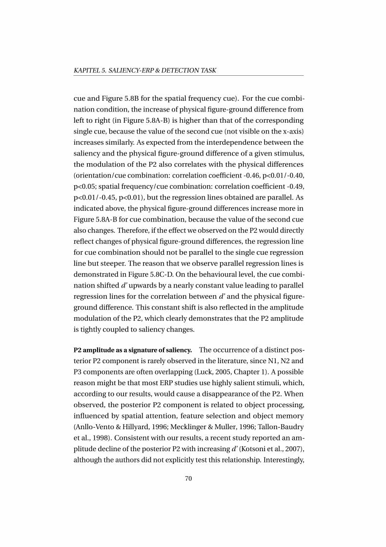
KAPITEL 5. SALIENCY-ERP & DETECTION TASK
cue and Figure 5.8B for the spatial frequency cue). For the cue combi-
nation condition, the increase of physical figure-ground difference from
left to right (in Figure 5.8A-B) is higher than that of the corresponding
single cue, because the value of the second cue (not visible on the x-axis)
increases similarly. As expected from the interdependence between the
saliency and the physical figure-ground difference of a given stimulus,
the modulation of the P2 also correlates with the physical differences
(orientation/cue combination: correlation coefficient -0.46, p<0.01/-0.40,
p<0.05; spatial frequency/cue combination: correlation coefficient -0.49,
p<0.01/-0.45, p<0.01), but the regression lines obtained are parallel. As
indicated above, the physical figure-ground differences increase more in
Figure 5.8A-B for cue combination, because the value of the second cue
also changes. Therefore, if the effect we observed on the P2 would directly
reflect changes of physical figure-ground differences, the regression line
for cue combination should not be parallel to the single cue regression
line but steeper. The reason that we observe parallel regression lines is
demonstrated in Figure 5.8C-D. On the behavioural level, the cue combi-
nation shifted d’ upwards by a nearly constant value leading to parallel
regression lines for the correlation between d’ and the physical figure-
ground difference. This constant shift is also reflected in the amplitude
modulation of the P2, which clearly demonstrates that the P2 amplitude
is tightly coupled to saliency changes.
P2 amplitude as a signature of saliency. The occurrence of a distinct pos-
terior P2 component is rarely observed in the literature, since N1, N2 and
P3 components are often overlapping (Luck, 2005, Chapter 1). A possible
reason might be that most ERP studies use highly salient stimuli, which,
according to our results, would cause a disappearance of the P2. When
observed, the posterior P2 component is related to object processing,
influenced by spatial attention, feature selection and object memory
(Anllo-Vento & Hillyard, 1996; Mecklinger &Muller, 1996; Tallon-Baudry
et al., 1998). Consistent with our results, a recent study reported an am-
plitude decline of the posterior P2 with increasing d’ (Kotsoni et al., 2007),
although the authors did not explicitly test this relationship. Interestingly,
70
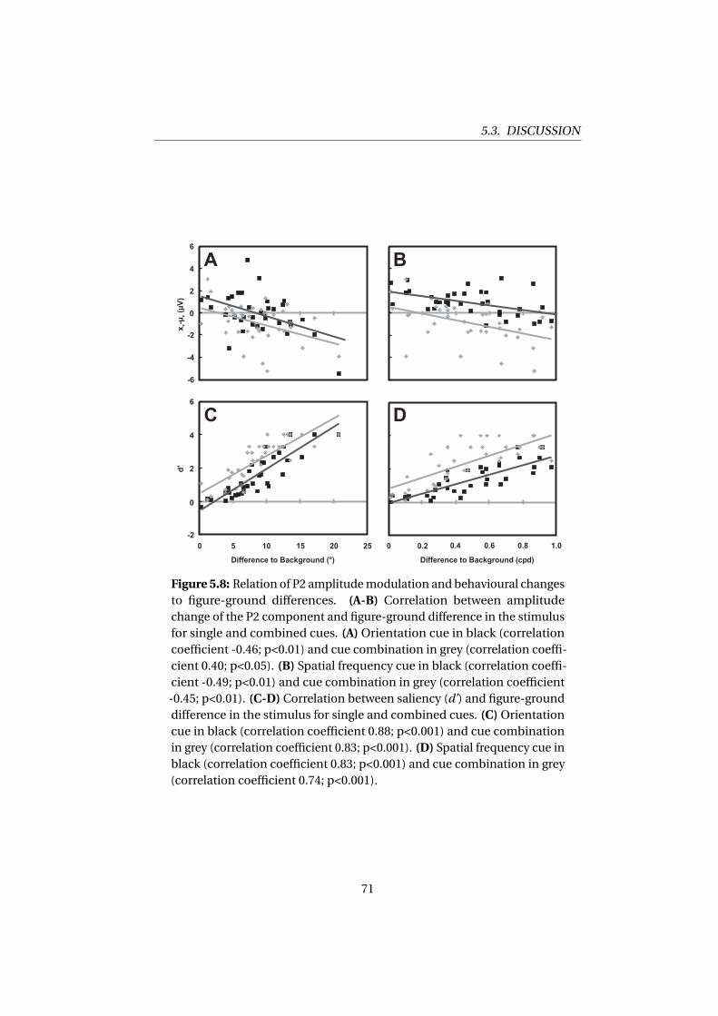
5.3. DISCUSSION
-6
-4
-2
0
2
4
6
0 5 10 15 20 25
Difference to Background (°)
x-μ
(μV
)s
s
-2
2
4
6
d’
0
0 0.2 0.4 0.6 0.8 1.0
Difference to Background (cpd)
A B
DC
Figure 5.8: Relation of P2 amplitudemodulation and behavioural changesto figure-ground differences. (A-B) Correlation between amplitudechange of the P2 component and figure-ground difference in the stimulusfor single and combined cues. (A)Orientation cue in black (correlationcoefficient -0.46; p<0.01) and cue combination in grey (correlation coeffi-cient 0.40; p<0.05). (B) Spatial frequency cue in black (correlation coeffi-cient -0.49; p<0.01) and cue combination in grey (correlation coefficient-0.45; p<0.01). (C-D) Correlation between saliency (d’) and figure-grounddifference in the stimulus for single and combined cues. (C)Orientationcue in black (correlation coefficient 0.88; p<0.001) and cue combinationin grey (correlation coefficient 0.83; p<0.001). (D) Spatial frequency cue inblack (correlation coefficient 0.83; p<0.001) and cue combination in grey(correlation coefficient 0.74; p<0.001).
71
KAPITEL 5. SALIENCY-ERP & DETECTION TASK
stimulus and paradigm of this study (common-onset visual masking)
profoundly differed from our study suggesting that the saliency-effect
on the P2 amplitude is robust across tasks and stimuli. This notion is
further supported by recent results from our lab, where subjects had to
identify the figure in a stimulus similar to the one reported here (Straube,
Grimsen & Fahle, submitted for publication). In this study, the same
effect of decreasing P2 amplitude with increasing d’ was observed, al-
though the task differed and the figure-ground differences required to
solve the identification task were much higher than for the detection task
described here. In summary, the P2 effect we find seems to be directly
correlated to saliency, an effect which is robust across tasks and stimulus
configurations. This finding supports the theory of a common saliency-
map (for a review see Treue, 2003) which is a cue-independent neural
representation of the object/target, formed by the combined responses of
selectively modulated neurons. The P2 modulation reported here could
well be a correlate of this saliency representation, since it is affected by
saliency irrespective the specific type of cue.
Alternatively, themodulation of the P2 could be interpreted as a corre-
late of top-down attentional resource allocation. Psychophysical studies
demonstrated that highly salient stimuli are effortlessly perceived (they
‘pop-out’ of the scene), while the same stimuli embedded in a display
with similar distractors will only be perceived when attention is directed
towards them (Nothdurft, 2000). Similarly, more difficult trials in our
study (i.e. trials of level 1) require more elaborate computation for an ap-
propriate behavioural result (correct answer). This increased processing
in more difficult trials might be mediated by attention. Then, increased
saliency means less attentional resource allocation, which is reflected in
the amplitude modulation of the posterior P2.
The neural resources performing this increased processing could
principally be situated in the earliest cortical visual areas. Neurons of the
primary visual cortex (V1) detect orientation and spatial frequency, but
interaction between these detectors is mandatory to segregate the figure
from the background. Either lateral interaction in V1 or an intermediate
72
5.3. DISCUSSION
area like the secondary visual cortex (V2) is required. It has been shown
that V2 is anatomically and functionally ideally suited for segregation
processes (Shipp & Zeki, 2002b,a). The feedback onto these very early
areas could principally originate in the lateral-occipital complex (LOC),
an area related to object processing. Indeed, it has been shown that
both, an early negative ERP-shift during processing of illusory contours
(Murray et al., 2002, 2004) and a later shift associated with closure of
contours (Doniger et al., 2000, 2001; Sehatpour et al., 2006) are located
in LOC. On the other hand, the detection of a figure can rely on local
differences or object parts in the stimulus, so the percept of the object
is not necessary for successful detection. Therefore, it is questionable if
the LOC is really involved in our paradigm, because the figure-ground
differences in our stimulus may not be sufficient to activate LOC.
Time-frequency analysis. All stimuli evoked a clear peak in the γ-band
around 100ms (see Figure 5.7). This activation of the γ-band is known to
occur strictly time-locked in object detection and discrimination tasks
(Busch et al., 2004, 2006; Senkowski & Herrmann, 2002). However, we
could not provide evidence that this early activation is sensitive to cue
condition or saliency, since there was no significant effect of any of these
on the γ-peak. Induced activations at higher latencies that have been
hypothesized to be involved in object representation (Tallon-Baudry &
Bertrand, 1999) were not observed in our study (compare Figure 5.7). As
argued above, the recognition of the figure was not necessary for success-
ful detection, so there was no real need for an object representation.
Similar to the reduction of the P2 amplitude, we observed a decrease
of θ-activation with increasing saliency and, akin to the P2 component,
modulations of the θ-band have been reported for short termmemory
and selective attention (Basar et al., 1999). The temporal resolution of a
wavelet analysis at such low frequencies is rather poor (i.e. at 4Hz a single
wavelet with 6 cycles has a time span of 1500ms), so the latency of the
θ-peak is necessarily imprecise. Nevertheless, the timing and direction of
changes observed are strikingly similar to the effect on the P2 observed
and a significant correlation was revealed. Furthermore, the P2 has a
73
KAPITEL 5. SALIENCY-ERP & DETECTION TASK
strong θ-component and the peak of the θ-band is mainly evoked (and
not induced), as was tested by analyzing θ-activity in the ERP. Therefore,
both effects strongly depend on each other, if they are not the same. In
summary, the effect of increased saliency is reflected by a decrease in P2
amplitude and a decrease in θ-activation.
The P3 component near perceptual threshold. About 150ms after the P2
effect, we observed a second modulation in the ERP which influenced
amplitude and latency of the posterior P3 component. The P3 is an ex-
tensively studied ERP component which is elicited in a large variety of
paradigms, and it has been shown that it is a major endogenous com-
ponent often related to decisionmaking and response certainty (for an
overview see Fabiani et al., 2000; Key et al., 2005; Luck, 2005, Chapter
1). Consistent with the literature (Picton, 1992; Polich & Kok, 1995), we
observe higher P3 amplitudes in trials where subjects were more certain
of their response. Accordingly, we find a positive correlation between
P3 amplitude and saliency, because -in our paradigm- higher response
certainty is at least partly mediated by higher saliency.
However, we also observe increasing P3 latencywith increasing saliency
as opposed to the classical view (Polich & Kok, 1995; Polich, 2004) that
postulates increased latencies for more difficult trials. Generally, the
figure in our stimulus is hardly visible and it has been shown that visual
noise distorts the P3 (McCarthy & Donchin, 1981). Most research on the
P3 has been performed with highly salient stimuli and hence our result
of increased latency may reflect the emergence of the P3 out of noise.
Possibly some classical characteristics of the P3, such as a negative corre-
lation between latency and amplitude, do not hold close to the perceptual
threshold.
5.4 Conclusions
In agreement with existing studies, we demonstrated that orientation
and spatial frequency interact as visual cues during figure detection.
Differences in the recorded potentials are strongly coupled with saliency
74
5.5. EXPERIMENTAL PROCEDURE
irrespective of the precise cue configuration, as revealed by an amplitude
decrease of the posterior P2 component and a reduction in θ-activity with
increasing saliency. No direct correlates of the physical stimulus changes
were observed, although we varied cue configuration (i.e. cue type and
number of cues) and cue intensity. This observation indicates that after
200ms, a target representation is established which is independent of the
precise type of cues. According to this view, it should make no difference
for the neural response if the figure-ground difference is increased by
higher cue intensity alone, an additional cue, or both.
5.5 Experimental Procedure
Subjects. Twelve undergraduate students (4 men, 8 women) aged be-
tween 21 and 28 years (mean 24.1, standard deviation 2.5) participated in
this study. All participants had normal or corrected-to-normal vision as
assessed by means of the Freiburger Visual Acuity Test (Bach, 1996) and
reported no neurological or psychiatric disorders. All subjects were naive
to task and stimulus. Each subject was informed about the nature and
the purpose of this study and gave written consent to participate. The
study was conducted in accordance with The Code of Ethics of the World
Medical Association (Declaration of Helsinki).
Task and stimulus. The stimulus consisted of a matrix of 33 x 25 Gabor
patches on a grey background, as demonstrated in Figure 5.1A, which
were presented at a distance of 70 cm on a Samsung Syncmaster 1100 MB
monitor with a resolution of 1600 x 1200 pixels at a frame rate of 100Hz.
The Gabor patches had a centre-to-centre distance of 1° of visual angle
and a size defined by the width of the Gaussian envelope of �=10 arcmin.
The target figure was part of this matrix with its elements differing from
the background either in orientation, spatial frequency, or both (cue
combination). The background elements had a spatial frequency of
3.5 cpd (cycles per degree) and an orientation of 36°.
In a two-alternative forced choice task, subjects had to indicatewhether
the figure occurred left or right of the vertical midline of themonitor. This
75
KAPITEL 5. SALIENCY-ERP & DETECTION TASK
position (left/right) was varied in a pseudorandomized order. Correct
detection was complicated by two further uncertainties: First, there was
a randomized positional jitter with the limitation that outer edges of the
figure were nomore eccentric than 7° of visual angle (in horizontal and
vertical direction) and that inner edges always intruded into the oppo-
site half of the visual field by 1° (Figure 5.1A). Second, the figure was
presented in one of eight possible versions (Figure 5.1A bottom). The
procedure of the experiment was as follows: A trial started with a fixation
period (300ms – black fixation point) followed by a blank screen (200ms).
Subsequently, the stimulus appeared for 80ms, again followed by a blank
screen (500ms). Finally, a small white square in the centre of the screen
indicated the answering period. There was no time limit for this period,
so subjects were free to answer whenever they wanted to (Figure 5.1B).
Auditory error-feedback was given (a 2000Hz tone for 100ms). The back-
ground colour of the monitor was grey during the whole sequence of
each trial.
Procedure
Training. Subjects were familiarized with the task and stimulus during
training sessions with a highly salient figure. These sessions were con-
ducted for both single cue conditions (30 trials per session), with the
figures’ Gabor elements oriented at 86° (i.e. 50° difference to the back-
ground) in the orientation condition, and with a spatial frequency above
5 cpd (i.e. 1.5 cpd difference to the background) in the spatial frequency
condition. The training session ended when observers reached at least 90
percent correct answers, otherwise the training was repeated. No subject
needed more than two repetitions.
Psychometric Functions of Single Cues. Saliency levels of the main exper-
iment were defined by the percent correct (pc) performance in the single
cue conditions. These performances were estimated by measuring the
psychometric functions for the detection of a figure purely defined by
a difference in orientation or else spatial frequency. The psychometric
76
5.5. EXPERIMENTAL PROCEDURE
function was characterized by its slope (�) and by the turning point (μ).
These parameters were used to evaluate the figure-ground difference
leading to the aspired performances (see below). The goodness of the
fit was evaluated with a chi-square test. Measurements were repeated in
case of insufficient fit.
To achieve an accurate measure of the psychometric function, we
used both an adaptive staircase procedure and themethod of constant
stimuli (MCS). First, we estimated thresholds –defined as the figure-
ground difference corresponding to 75 percent correct performance–
and slope of the psychometric function using the QUESTmethod (Wat-
son & Pelli, 1983) with 50 trials. Second, we validated these results using
aMCS by pseudorandomizing five values of the estimated function (pa-
rameters corresponding to a correct performance of 55%, 65%, 75%,
85% and 95%) andmeasuring the performance corresponding to these
values with 30 trials per value (i.e. 150 trials per MCS).
The psychometric functions thus measured were then used for the
main experiment.
Main Experiment. The three conditions of the main experiment were:
detection of a figure defined by a figure-ground difference in i) orienta-
tion (single cue), ii) spatial frequency (single cue) or iii) orientation and
spatial frequency (cue combination). Each condition was tested with
three levels of difficulty, which were derived from the psychometric func-
tions of the single cue conditions (see above). These levels were defined
as stimuli corresponding to a correct performance of 55%, 76% and 98%,
respectively. The values of both cues were combined for the correspond-
ing level in the cue combination condition. For instance, on level 1 of the
cue combination condition, the Gabor patches of the figure displayed the
figure-ground difference corresponding to level 1 regarding both single
cue conditions. Each configuration (condition x level) was repeated 100
times and presented in a pseudo-randomized order. Therefore the main
experiment consisted of three runs (one run=one condition, 300 trials
per run), with a sequence counterbalanced between subjects. All partic-
77
KAPITEL 5. SALIENCY-ERP & DETECTION TASK
ipants were instructed to blink only during the answer phase to avoid
blink artefacts in the time span of the ERP.
Control Experiment – Figure present or not? Eight subjects performed the
control experiment in the same session. Stimulus, sequence and position-
ing of the figure were the same as in the previous experiments, but here
the stimulus either contained a figure or else none. Subjects reported
the presence of the figure in a yes-no detection paradigm. When a figure
was present, it consisted of the single cue differences (either spatial fre-
quency or orientation) corresponding to level 3. Trials without the figure
contained only the background elements described above. The control
experiment again consisted of 300 trials (100 trials per cue condition plus
100 trials without any figure).
Electrophysiological Recording. The electroencephalogram (EEG) was
recorded in the main experiment from 25 recording sites (FP1, FP2, F7,
F3, Fz, F4, F8, T7, C3, Cz, C4, T8, P7, P3, Pz, P4, P8, PO7, PO3, POz,
PO4, PO8, O1, Oz, O2) chosen from standard electrode positions (Ameri-
can Electroencephalographic Society, 1994) using Ag/AgCl sintered elec-
trodes placed in an electrode cap (Easycap, Herrsching-Breitbrunn). Elec-
trode Cz served as reference during data acquisition. The data were
re-referenced off-line to the averaged earlobes (A1 and A2) to allow a
direct comparison with published studies. Electrode impedance was
kept below 10k�. Eye movements, such as blinks, were monitored with
two additional electrodes above and lateral to the left eye. The electrode
potentials were amplified using a Nihon Kohden system (Neurofax EEG-
1100). During recording, a time constant of 0.3 s (cutoff frequency: 0.5Hz)
and a high-frequency cutoff of 120Hz were used. The EEG was digitized
at a sampling rate of 500Hz.
Data Analysis
Performancemeasures and independent summationmodel. The work by
Meinhardt and colleagues demonstrated that orientation and spatial
78
5.5. EXPERIMENTAL PROCEDURE
frequency interact as visual cues for detection and identification (Mein-
hardt & Persike, 2003; Meinhardt et al., 2004, 2006). Interaction during
cue combination can be tested by comparing the actual performance
for combined cues with the prediction of an independent summation
assumption of both single cues. Under this assumption, provided by
signal detection theory, independent cue processing should produce a
combined performance (d ′⊥) that is based on the performances of the
single cues alone, according to
d ′⊥ =
√(d ′
f )2+ (d ′
φ)2, (5.1)
(Ashby & Townsend, 1986; Green & Swets, 1988, p.271 ff.; Macmillan &
Creelman, 1991, p. 240 ff.). The parameter d’ is a measure of the dis-
tance between the noise and signal distributions, hence an increase in
d’ denotes an increase in performance. The two single-cue distributions
(index f for spatial frequency cue, indexφ for orientation cue) are orthog-
onal to each other in case of independent summation (d ′⊥) (Tanner, 1956),
so the resulting perceptual object saliency is defined by the Euclidean
distance between them.
Percent correct performance in a 2-alternative forced choice task and
d’ are related by
d ′ =�2∗Θ−1(pc). (5.2)
Here,Φ is the normal distribution function, and thereforeΦ−1(pc) givesthe z-score of the percent correct value (Macmillan & Creelman, 1991,
p. 124 ff.). Due to this direct relationship, we can rescale performance
values to d’ and evaluate the prediction of the independent summation
model (see Equation 5.1).
In the case of perfect performance (100%-correct) the value of d’
becomes infinite. In order to compute a finite value of d’ in this case,
we set its value to a maximum of 4.0, which corresponds to a correct
performance of 99.8% according to the relationship in Equation 5.2.
79
KAPITEL 5. SALIENCY-ERP & DETECTION TASK
Event-related potentials. ERPs were investigated in a time span from
-100ms to 500ms relative to stimulus onset, filtered with a 30Hz (slope
24dB/oct) low-pass filter prior to averaging. Trials with blink artefacts,
large eye movements, extensive muscle activity or other noise transients
within this time span were rejected automatically on all recorded chan-
nels through an amplitude limitation of ±70μV (5 subjects at ±100μV)
and by visual inspection. Further control of eyemovement was not neces-
sary, since saccades to specifically search for the figure were not possible
due to the short stimulus duration (80ms). Only trials with correctly
detected stimuli were included in the analysis. Remaining trials after arte-
fact rejection for each level (mean and standard deviation) were: 63 trials
(sd 7 trials) for level 1, 81 trials (sd 9 trials) for level 2 and 88 trials (sd
3 trials) for level 3.
Themean signal of the 100ms time window prior to stimulus onset
served for baseline correction. Filtering, artefact rejection and ERP gener-
ation were performed using BESA 5.1.8 software (MEGIS Software GmbH,
Munich). Evaluation of grand average ERPs was carried out with in-house
software usingMatlab (Release 12.1, TheMathWorks Inc., Massachusetts).
Amplitudes were defined as distance to baseline.
Time-frequency analysis. Trials with artefacts identified in the ERP anal-
ysis were also not included in the time-frequency analysis, which was
computed over a time span from -1500 ms to 1250 ms relative to stimulus
onset to avoid border artefacts. We used aMorlet basedwavelet transform
with a width of 6 cycles for the inspection of power changes of defined
frequencies (4–80Hz). The core routine was provided by Torrence and
Compo (1998). Only trials with correctly identified stimuli were included
in the analysis (see above). In contrast to the ERP analysis, the data were
not filtered to avoid filter distortions. We investigated normalized me-
dian power values of total activity (evoked and induced – for details see
Herrmann et al., 2005). The procedure was as follows: For each subject
separately, we computed the power values (in μV²) in each trial for each
frequency (f ) and summarized all trials by taking the median power at
each frequency and time point. Moreover, we normalized the power
80
5.5. EXPERIMENTAL PROCEDURE
value (Pf ) at each time point t by the mean of the baseline power (P̄0f )
according to
Pnormf (t )=
Pf (t )− P̄0f
P̄0f
. (5.3)
Therefore the resulting normalized power value (Pnormf ) at time has no
unit and represents the activity in proportion to baseline activity. As
baseline, we used the time window 750ms prior to stimulus onset. Since
the normalization factor (P̄0f ) here is frequency-dependent, the normal-
ization also accounts for the fact that high frequencies have less power in
the EEG than low frequencies do. Hence, the normalized power values
represent the frequency-specific increase compared to baseline power.
Finally, the normalized data were averaged over all subjects. Due to
nine experimental configurations (condition x level) we obtained nine
time-frequency plots for each electrode.
Statistics. The statistical analysis was performed using SPSS 15.0 (SPSS
Inc., Chicago). All results (performance, ERPs and time-frequency analy-
sis) were validated by using repeatedmeasurement ANOVAs. Wherever
appropriate, p-values were adjusted by Greenhouse-Geisser corrections.
Pairwise comparisons were conducted by using post-hoc t-tests. The cor-
relations computed in this study report Pearson’s correlation coefficient.
Acknowledgements
We would like to thank C. Grimsen for invaluable support throughout the
project.
81

Kapitel 6
Electrophysiological correlates of
figure-ground segregation
directly reflect perceptual
saliency
Sirko Straube, Cathleen Grimsen &Manfred Fahle
Abstract
During visual processing, we constantly separate figures from their back-
ground. It is currently under debate whether multiple figure cues are
processed independently. We investigated the influence of different cue
configurations on the human EEG in a figure identification task. In a
Gabor matrix, either spatial frequency, orientation or both (cue combi-
nation) served as figure cues. Psychophysically, we observed an inter-
action for cue combination. Combining psychophysics with ERP and
time-frequency analysis, we show that the neural response at a latency
of 200 ms reflects perceptual saliency rather than physical cue contrast.
Increasing saliency caused a negative shift of the posterior P2 compo-
nent coinciding with a decrease in the posterior θ-band (4-8Hz), while
83
KAPITEL 6. SALIENCY-ERP & IDENTIFICATION TASK
decision confidence was reflected in the posterior P3. We demonstrate
that visual cues interact for a percept that is non-linearly related to the
physical figure-ground properties.
6.1 Introduction
When looking at a visual scene, we simultaneously identify different ob-
jects without caring about the visual features underlying this percept.
However, we often recognize objects based on a conjunction of cues
instead of using only one single visual cue (e.g. depth, colour or orienta-
tion in space). The percept of the object is coherent, meaning that the
information from various cues is integrated by the visual system.
To what extent is it easier to perceive an object defined by multiple
cues instead of one defined by a single cue? Several behavioural studies
dealing with cue combination tried to answer this important question
with the result that combination seems to depend on task and cue type.
Therefore, the amount of behavioural benefit from cue combination is
still under debate, with the majority of studies observing cue interaction
(Abele & Fahle, 1995; Kubovy et al., 1999; Kubovy & Cohen, 2001; Mein-
hardt & Persike, 2003; Meinhardt et al., 2004, 2006; van Mierlo et al., 2007;
Nothdurft, 2000; Persike & Meinhardt, 2006; Rivest & Cavanagh, 1996),
while others find independent processing (Leonards & Singer, 2000; Pash-
ler, 1988; Phillips & Craven, 2000; Phillips, 2001; Treisman & Gelade, 1980;
Tsujimoto & Tayama, 2004). A deeper understanding of the underly-
ing processes could be provided by electrophysiological measurements
which allow to link physical stimulus properties and behavioural mea-
surements with the timing of the neural response and are therefore ideal
to examine the effect of cue combination on figure-ground segregation.
Although a number of electrophysiological studies investigated the effect
of figure-ground segregation on the electroencephalogram (EEG), there
is no study specifically testing the effect of cue combination. Hence, an
electrophysiological correlate of the combination process is still missing.
At least it is known from a lot of studies that segregation of textures and
figures causes a similar segregation-specific negative potential shift for a
84
6.1. INTRODUCTION
number of cues, suggesting that objects are recognized by the visual sys-
tem with a high temporal and spatial congruence across cue types. This
shift occurs between 100 ms and 300 ms in the event-related potential
(ERP) and was termed the texture-segregation visual evoked potential
(tsVEP – Bach &Meigen, 1992, 1997; Bach et al., 2000; Caputo & Casco,
1999; Fahle et al., 2003). Similarly, a contour-specific negative response
was found for contour integration paradigms (Mathes et al., 2006; Mathes
& Fahle, 2007), whereas later parts (maximally at 290 ms) were associ-
ated with closure processes (Doniger et al., 2000, 2001). Even when the
contour was not physically present (i.e. it was illusory), an early negative
modulation of the ERP was reported (Herrmann & Bosch, 2001; Murray
et al., 2002, 2006). Although these potentials occur partly at different
latencies in the ERP and likely reflect different aspects of object recog-
nition, it seems to be a common observation that the ERP is negatively
modulated when objects are recognized.
An alternative way of looking at the electrophysiological response to
a given stimulus is the investigation of specific frequency modulations
in the EEG over time. Here, segregation-specific activity has been found
in the γ-band (Eckhorn et al., 1988) and it has been shown that an early
evoked activation in the γ-band is sensitive to stimulus properties in
object detection and discrimination (Busch et al., 2004, 2006; Senkowski
&Herrmann, 2002), while an induced activation at higher latencies seems
to be involved in object representation (Tallon-Baudry & Bertrand, 1999).
Both effects, the segregation-specific negativity of the ERP and the mod-
ulation of the γ-band are closely related to figure-ground segregation,
which suggests that bothmay be sensitive to cue combination and/or the
corresponding effect on the saliency of an object.
In the present study we specifically investigate for the effect of cue
combination and the related saliency changes on the human EEG (both,
ERPs and specific frequency bands). Combining signal-detection the-
ory and electrophysiology, we tested how the identification of a figure is
altered by the underlying cue configuration, specifically by comparing
single cues with cue combination, and how these changes influence the
85
KAPITEL 6. SALIENCY-ERP & IDENTIFICATION TASK
electrophysiological data. The paradigm is inspired by work fromMein-
hardt and colleagues who found an interaction in psychophysical tests
when combining orientation and spatial frequency as visual cues (Mein-
hardt et al., 2004, 2006). They also reported differences in cue interaction
between detection and identification tasks. Here, we concentrate on iden-
tification by using a figure discrimination task requiring identification of
the target. Segregation of the figure from its background is not sufficient
to solve this task but a classification is required. According to the results
of Meinhardt et al., we expect a synergy effect for cue combination on the
behavioural level. Our study focuses on the earliest electrophysiological
changes (ERP and/or time frequency analysis) that can be attributed
either to the physical properties of the stimulus and/or the percept. Due
to the fact that orientation and spatial frequency interact as visual cues
during figure-ground segregation, the expected changes should occur
in the time range of the segregation specific negativity of the ERP (i.e.
between 100ms and 300ms). As outlined above, we also consider the
γ-band (evoked and induced activity) as a candidate, possibly reflecting
the cue configuration of the target or the perceived saliency of the figure.
6.2 Materials andMethods
Subjects
Twelve undergraduate students (6 men, 6 women) aged between 22 and
27 (mean 23.7, sd 1.3) participated in this study. All participants had nor-
mal or corrected-to-normal vision as assessed bymeans of the Freiburger
Visual Acuity Test (Bach, 1996) and reported no history of neurological or
psychiatric disorders. Each subject was informed about the nature and
the purpose of this study and gave written consent to participate. The
study was conducted in accordance with The Code of Ethics of the World
Medical Association (Declaration of Helsinki) and approved by the local
ethics committee.
86
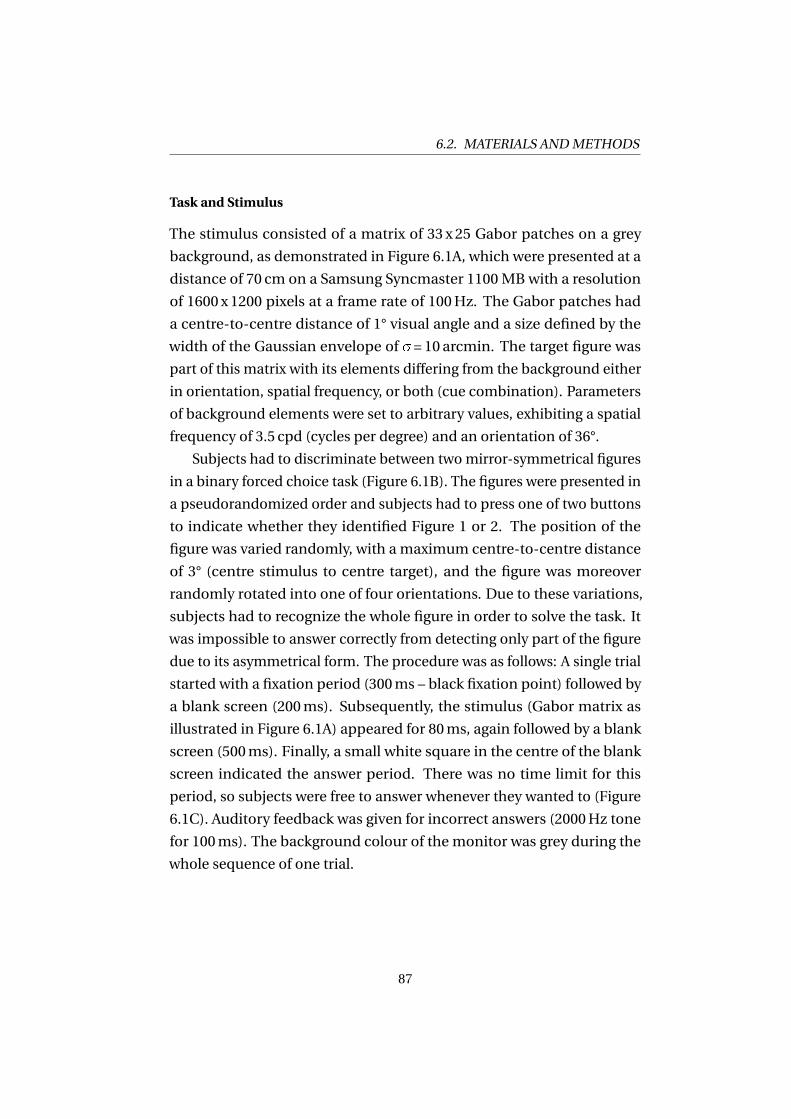
6.2. MATERIALS AND METHODS
Task and Stimulus
The stimulus consisted of a matrix of 33 x 25 Gabor patches on a grey
background, as demonstrated in Figure 6.1A, which were presented at a
distance of 70 cm on a Samsung Syncmaster 1100MBwith a resolution
of 1600 x 1200 pixels at a frame rate of 100Hz. The Gabor patches had
a centre-to-centre distance of 1° visual angle and a size defined by the
width of the Gaussian envelope of �=10arcmin. The target figure was
part of this matrix with its elements differing from the background either
in orientation, spatial frequency, or both (cue combination). Parameters
of background elements were set to arbitrary values, exhibiting a spatial
frequency of 3.5 cpd (cycles per degree) and an orientation of 36°.
Subjects had to discriminate between twomirror-symmetrical figures
in a binary forced choice task (Figure 6.1B). The figures were presented in
a pseudorandomized order and subjects had to press one of two buttons
to indicate whether they identified Figure 1 or 2. The position of the
figure was varied randomly, with a maximum centre-to-centre distance
of 3° (centre stimulus to centre target), and the figure was moreover
randomly rotated into one of four orientations. Due to these variations,
subjects had to recognize the whole figure in order to solve the task. It
was impossible to answer correctly from detecting only part of the figure
due to its asymmetrical form. The procedure was as follows: A single trial
started with a fixation period (300ms – black fixation point) followed by
a blank screen (200ms). Subsequently, the stimulus (Gabor matrix as
illustrated in Figure 6.1A) appeared for 80ms, again followed by a blank
screen (500ms). Finally, a small white square in the centre of the blank
screen indicated the answer period. There was no time limit for this
period, so subjects were free to answer whenever they wanted to (Figure
6.1C). Auditory feedback was given for incorrect answers (2000Hz tone
for 100ms). The background colour of the monitor was grey during the
whole sequence of one trial.
87
KAPITEL 6. SALIENCY-ERP & IDENTIFICATION TASK
Fixation 300 ms
Blank 200 ms
Stimulus 80 ms
Blank 500 ms
Answer +Feedback
A B
C
Figure 1 Figure 2
0°
90°
180°
270°
Rotation
Figure 6.1: Stimulus and task. (A) Amatrix of Gabor elements containinga figure (shown here is the cue combination condition). The dashedline is shown for illustration purposes only and was not present in theoriginal stimulus. All background elements had the same orientation andspatial frequency. Figure elements differed either in orientation, spatialfrequency or both (cue combination). (B) Subjects had to discriminatebetween two mirror symmetrical figures, which were presented randomlyat one of four orientations. Figure 1 is rotated counterclockwise (indicatedby arrow), while Figure 2 is rotated clockwise, so that opposite pairs arealways mirror images. (C) Sequence of one trial. The white square at theend of each trial indicated the answering period, which had no time limit.Auditory error feedback was given.
88
6.2. MATERIALS AND METHODS
Procedure
Training. To ensure that all subjects were able to identify the figure prop-
erly, they were trainedwith a highly salient figure prior to the experiments.
Training sessions were conducted for both single cue conditions (30 tri-
als per session), with the figures’ Gabor elements having an orientation
of above 86° (i.e. 50° difference to the background) in the orientation
condition and a spatial frequency above 5 cpd (i.e. 1.5 cpd difference
to the background) in the spatial frequency condition, respectively. If
the subject reached an accuracy of at least 90 percent correct answers,
the training session was finished, otherwise it was repeated. No subject
needed more than one repetition.
Psychometric Functions of SingleCues. The levels of difficulty in themain
experiment were defined by the percent correct (pc) performance in the
single cue conditions. Performance was estimated by measuring the
psychometric functions for the identification of a figure defined purely
by a difference in orientation or else spatial frequency. Any parameter-
performance pair can be evaluated in this way due to the fact that the
psychometric function is characterized by the location of a perceptual
threshold and by its slope.
To achieve an accurate measure of the psychometric function, we
sequentially used both an adaptive staircase procedure and the method
of constant stimuli (MCS). First, we estimated the threshold – defined as
the figure-ground difference corresponding to 75 percent correct perfor-
mance – and the slope of the psychometric function using the QUEST
method (Watson & Pelli, 1983) with 50 trials. Second, we validated these
results with the MCS by taking 5 values of the estimated function (param-
eters corresponding to a correct performance of 55%, 65%, 75%, 85%
and 95%) presented pseudorandomized with 30 trials per configuration,
which leads to 150 trials per MCS.
The psychometric functions thus measured were then used for the
main experiment.
89
KAPITEL 6. SALIENCY-ERP & IDENTIFICATION TASK
Main Experiment. Three conditions were tested in the main experiment:
identification of a figure defined by a figure-ground difference in i) orien-
tation (single cue), ii) spatial frequency (single cue) or iii) orientation and
spatial frequency (cue combination). Each of these conditions was tested
with three levels of difficulty, which were derived from the psychometric
functions of the single cue conditions (see above). These levels were de-
fined as stimuli corresponding to a correct performance of 55%, 76% and
98%, respectively. In the cue combination condition, figure-ground dif-
ferences were defined by the superposition of the two single cue stimuli
of the corresponding levels. For instance, on level 1 of the cue combi-
nation condition, the Gabor patches of the figure had a figure-ground
difference corresponding to level 1 regarding both single cue conditions.
Each configuration (condition x level) was repeated 100 times and pre-
sented in pseudo-randomized order. Therefore, the main experiment
consisted of three runs (one run=one condition, 300 trials per run), with
the sequence counterbalanced between subjects. All participants were
instructed only to blink during the answer phase to avoid blink artefacts
in the time span of the ERP.
Control Experiment – Figure versus Background. In a separate session,
five of the subjects that took part in the main experiment performed
a control experiment. The purpose of this experiment was to evaluate
whether the figure in our stimulus by itself caused a segregation-specific
negative shift in the ERP and whether the rarely observed P2 component
(see Results and Discussion) is also observed in the pure background
stimulus with a slightly modified task.
Stimulus, sequence and positioning of the figure were the same as in
the previous experiments, but here the stimulus either contained a figure
or else none. Subjects reported the presence of the figure in a yes-no
detection paradigm. When a figure was present, it consisted of the single
cue differences (either spatial frequency or orientation) corresponding to
level 3. Trials without the figure contained only the background elements
described above. The control experiment again consisted of 300 trials
(100 trials per cue condition plus 100 trials without any figure).
90
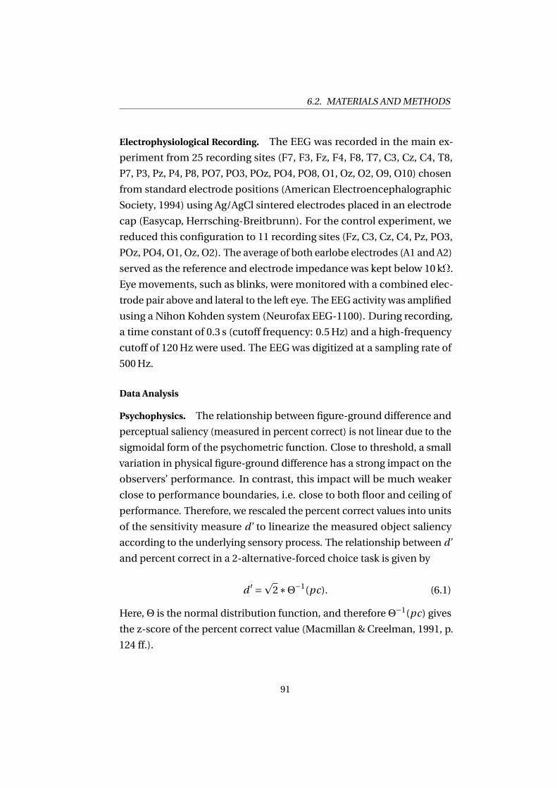
6.2. MATERIALS AND METHODS
Electrophysiological Recording. The EEG was recorded in the main ex-
periment from 25 recording sites (F7, F3, Fz, F4, F8, T7, C3, Cz, C4, T8,
P7, P3, Pz, P4, P8, PO7, PO3, POz, PO4, PO8, O1, Oz, O2, O9, O10) chosen
from standard electrode positions (American Electroencephalographic
Society, 1994) using Ag/AgCl sintered electrodes placed in an electrode
cap (Easycap, Herrsching-Breitbrunn). For the control experiment, we
reduced this configuration to 11 recording sites (Fz, C3, Cz, C4, Pz, PO3,
POz, PO4, O1, Oz, O2). The average of both earlobe electrodes (A1 and A2)
served as the reference and electrode impedance was kept below 10k�.
Eye movements, such as blinks, were monitored with a combined elec-
trode pair above and lateral to the left eye. The EEG activity was amplified
using a Nihon Kohden system (Neurofax EEG-1100). During recording,
a time constant of 0.3 s (cutoff frequency: 0.5Hz) and a high-frequency
cutoff of 120Hz were used. The EEG was digitized at a sampling rate of
500Hz.
Data Analysis
Psychophysics. The relationship between figure-ground difference and
perceptual saliency (measured in percent correct) is not linear due to the
sigmoidal form of the psychometric function. Close to threshold, a small
variation in physical figure-ground difference has a strong impact on the
observers’ performance. In contrast, this impact will be much weaker
close to performance boundaries, i.e. close to both floor and ceiling of
performance. Therefore, we rescaled the percent correct values into units
of the sensitivity measure d’ to linearize the measured object saliency
according to the underlying sensory process. The relationship between d’
and percent correct in a 2-alternative-forced choice task is given by
d ′ =�2∗Θ−1(pc). (6.1)
Here,Θ is the normal distribution function, and thereforeΘ−1(pc) givesthe z-score of the percent correct value (Macmillan & Creelman, 1991, p.
124 ff.).
91
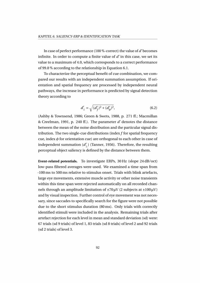
KAPITEL 6. SALIENCY-ERP & IDENTIFICATION TASK
In case of perfect performance (100%-correct) the value of d’ becomes
infinite. In order to compute a finite value of d’ in this case, we set its
value to a maximum of 4.0, which corresponds to a correct performance
of 99.8% according to the relationship in Equation 6.1.
To characterize the perceptual benefit of cue combination, we com-
pared our results with an independent summation assumption. If ori-
entation and spatial frequency are processed by independent neural
pathways, the increase in performance is predicted by signal detection
theory according to
d ′⊥ =
√(d ′
f )2+ (d ′
φ)2, (6.2)
(Ashby & Townsend, 1986; Green & Swets, 1988, p. 271 ff.; Macmillan
& Creelman, 1991, p. 240 ff.). The parameter d’ denotes the distance
between the mean of the noise distribution and the particular signal dis-
tribution. The two single-cue distributions (index f for spatial frequency
cue, index φ for orientation cue) are orthogonal to each other in case of
independent summation (d ′⊥) (Tanner, 1956). Therefore, the resulting
perceptual object saliency is defined by the distance between them.
Event-related potentials. To investigate ERPs, 30Hz (slope 24dB/oct)
low-pass filtered averages were used. We examined a time span from
-100ms to 500ms relative to stimulus onset. Trials with blink artefacts,
large eye movements, extensive muscle activity or other noise transients
within this time span were rejected automatically on all recorded chan-
nels through an amplitude limitation of ±70μV (2 subjects at ±100μV)
and by visual inspection. Further control of eyemovement was not neces-
sary, since saccades to specifically search for the figure were not possible
due to the short stimulus duration (80ms). Only trials with correctly
identified stimuli were included in the analysis. Remaining trials after
artefact rejection for each level in mean and standard deviation (sd) were:
67 trials (sd 9 trials) of level 1, 83 trials (sd 8 trials) of level 2 and 92 trials
(sd 2 trials) of level 3.
92
6.2. MATERIALS AND METHODS
The mean signal of the 100ms time window prior to stimulus on-
set served for baseline correction. The ERPs were sorted according to
stimulus level and to the observers’ answers. Filtering, artefact rejection
and ERP generation were carried out using BESA 5.1.8 (MEGIS Software
GmbH, Munich). Grand average ERPs, amplitude and latency measure-
ments of components were computed with in-house software using Mat-
lab (Release 12.1, The MathWorks Inc., Massachusetts). Amplitudes were
defined as distance to baseline.
Time-frequency analysis. AMorlet based wavelet transform with a width
of 6 cycles was used for the inspection of power changes within defined
frequency bands (4–80Hz). The core routine was provided by Torrence
and Compo (1998). Trials with artefacts identified in the ERP analysis
were again not included in the time-frequency analysis, which was com-
puted over a time span between -1500ms and 1250ms relative to stimulus
onset to avoid border artefacts. Only trials with correctly identified stim-
uli were included in the analysis. In contrast to the ERP analysis, the
data were not filtered. We investigated normalized median power values
of total activity (evoked and induced – for details see Herrmann et al.,
2005). The procedure was as follows: For each subject separately, we
computed the power values (in μV²) in each trial for each frequency (f )
and summarized all trials by taking the median power at each frequency
and point in time. Moreover, we normalized the power value (Pf ) at each
time point t by the mean of the baseline power (P̄0f ) according to
Pnormf (t )=
Pf (t )− P̄0f
P̄0f
. (6.3)
Therefore the resulting normalized power value (Pnormf ) at time has no
unit and represents the activity relative to baseline. As baseline, we
used the time window 750ms prior to stimulus onset. Since the nor-
malization factor (P̄0f ) is frequency-dependent, the normalization also
accounts for the fact that high frequencies have less power in the EEG
93
KAPITEL 6. SALIENCY-ERP & IDENTIFICATION TASK
than low frequencies. Hence, the normalized power values represent the
frequency-specific increase compared to baseline power.
Finally, the normalized data were averaged over all subjects. We ob-
tained nine time-frequency plots for each electrode for the nine experi-
mental configurations (condition x level).
Statistics. Statistical analysis was performed using SPSS 12.0 (SPSS Inc.,
Chicago). All results (performance, ERPs and time-frequency analysis)
were validated by using repeatedmeasurement ANOVAs. Wherever ap-
propriate, p-values were adjusted by Greenhouse–Geisser corrections.
Pairwise comparisons were conducted by using post-hoc t-tests. The cor-
relations computed in this study report Pearson’s correlation coefficient.
6.3 Results
Psychophysics. The measurement of the psychometric functions for
both single cue conditions in the main experiment revealed similar
thresholds (points of 75 %-correct performance) for all subjects, which
lay at 50.8° (sd 2.2°) for the orientation and at 4.7 cpd (sd 0.2 cpd) for
the spatial frequency condition. Figure 6.2 shows an increase in per-
formance from levels 1 to 3 in all conditions. Furthermore, both single
cue conditions had similar saliencies at all levels, with level 1 beneath
threshold (d’<1.0), level 2 slightly above threshold (1.0<d’<2.0), and level 3
way above threshold (d’>2.0) and close to the performance limit. A two
factorial ANOVA for repeated measurements showed a significant main
effect for both level (F(2,22)=70.0, p<0.001) and condition (F(2,22)=14.2,
p<0.001), whereas we observed no significant interactions (F(4,44)=2.3,
p=0.08). Pairwise comparisons of the three conditions on each level
yielded no differences between the two single cue performances (two-
tailed t-test – level 1: p=0.35; level 2: p=0.19; level 3: p=0.57), while there
was a significant improvement for the cue combination (one-tailed t-test
– true for both single cues: level 1: p<0.01; level 2: p<0.001; level 3: p<0.05).
Hence, the combination of both cues increased object-saliency compared
to single cues on all levels. On levels 1 and 2, the perceptual improve-
94
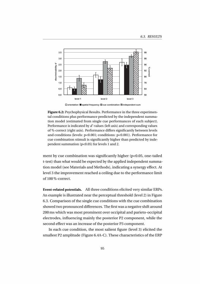
6.3. RESULTS
0.0
0.5
1.0
1.5
2.0
2.5
3.0
3.5
level 1 level 2 level 3
orientation spatial frequency cue combination independent sum
50
64
76
86
92
96
98
99
dis
crim
inab
ilit
yd
’
%-c
orrect
Figure 6.2: Psychophysical Results. Performance in the three experimen-tal conditions plus performance predicted by the independent summa-tion model (estimated from single cue performances of each subject).Performance is indicated by d’-values (left axis) and corresponding valuesof %-correct (right axis). Performance differs significantly between levelsand conditions (levels: p<0.001; conditions: p<0.001). Performance forcue combination stimuli is significantly higher than predicted by inde-pendent summation (p<0.05) for levels 1 and 2.
ment by cue combination was significantly higher (p<0.05, one-tailed
t-test) than what would be expected by the applied independent summa-
tionmodel (see Materials andMethods), indicating a synergy effect. At
level 3 the improvement reached a ceiling due to the performance limit
of 100%-correct.
Event-related potentials. All three conditions elicited very similar ERPs.
An example is illustrated near the perceptual threshold (level 2) in Figure
6.3. Comparison of the single cue conditions with the cue combination
showed two pronounced differences. The first was a negative shift around
200ms which was most prominent over occipital and parieto-occipital
electrodes, influencing mainly the posterior P2 component, while the
second effect was an increase of the posterior P3 component.
In each cue condition, the most salient figure (level 3) elicited the
smallest P2 amplitude (Figure 6.4A-C). These characteristics of the ERP
95
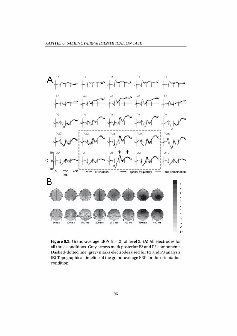
KAPITEL 6. SALIENCY-ERP & IDENTIFICATION TASK
Figure 6.3: Grand-average ERPs (n=12) of level 2. (A) All electrodes forall three conditions. Grey arrows mark posterior P2 and P3 components.Dashed-dotted line (grey) marks electrodes used for P2 and P3 analysis.(B) Topographical timeline of the grand-average ERP for the orientationcondition.
96
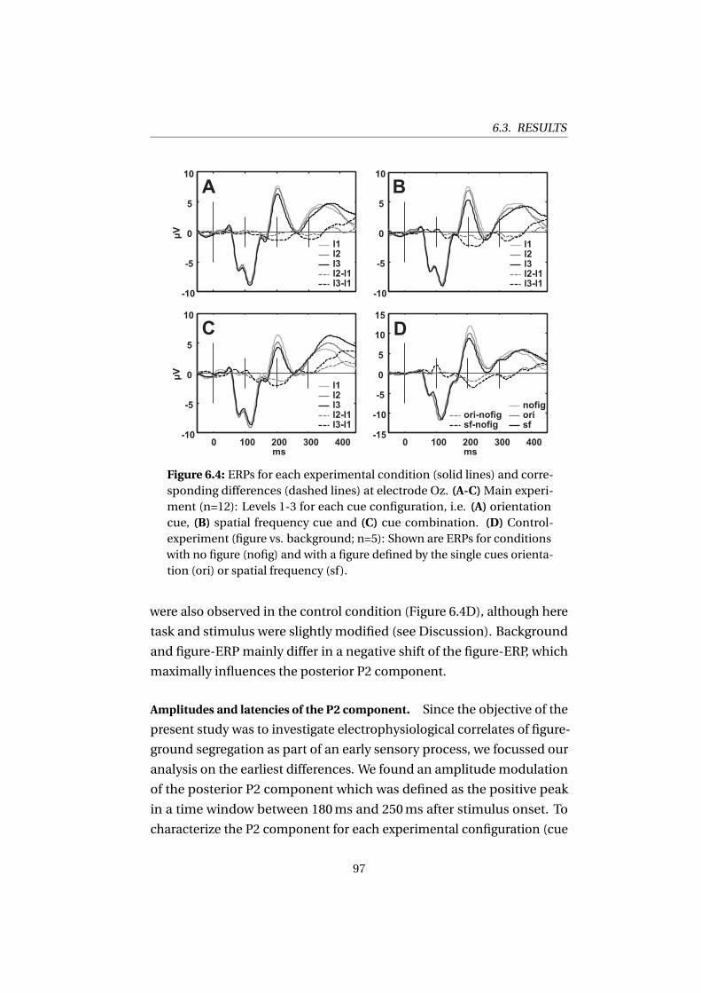
6.3. RESULTS
-10
-5
0
5
10μ
V
l1
l2
l3
l2-l1
l3-l1
A
0 100 200 300 400-10
-5
0
5
10
ms
μV
l1
l2
l3
l2-l1
l3-l1
C
0 100 200 300 400-15
-10
-5
0
5
10
15
ms
nofig
ori
sf
ori-nofig
sf-nofig
D
l1
l2
l3
l2-l1
l3-l1
B
-10
-5
0
5
10
Figure 6.4: ERPs for each experimental condition (solid lines) and corre-sponding differences (dashed lines) at electrode Oz. (A-C)Main experi-ment (n=12): Levels 1-3 for each cue configuration, i.e. (A) orientationcue, (B) spatial frequency cue and (C) cue combination. (D) Control-experiment (figure vs. background; n=5): Shown are ERPs for conditionswith no figure (nofig) and with a figure defined by the single cues orienta-tion (ori) or spatial frequency (sf).
were also observed in the control condition (Figure 6.4D), although here
task and stimulus were slightly modified (see Discussion). Background
and figure-ERPmainly differ in a negative shift of the figure-ERP, which
maximally influences the posterior P2 component.
Amplitudes and latencies of the P2 component. Since the objective of the
present study was to investigate electrophysiological correlates of figure-
ground segregation as part of an early sensory process, we focussed our
analysis on the earliest differences. We found an amplitude modulation
of the posterior P2 component which was defined as the positive peak
in a time window between 180ms and 250ms after stimulus onset. To
characterize the P2 component for each experimental configuration (cue
97
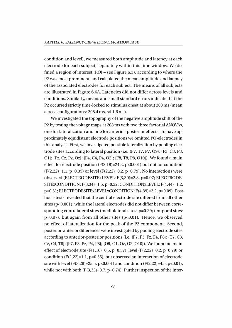
KAPITEL 6. SALIENCY-ERP & IDENTIFICATION TASK
condition and level), wemeasured both amplitude and latency at each
electrode for each subject, separately within this time window. We de-
fined a region of interest (ROI – see Figure 6.3), according to where the
P2 was most prominent, and calculated the mean amplitude and latency
of the associated electrodes for each subject. Themeans of all subjects
are illustrated in Figure 6.6A. Latencies did not differ across levels and
conditions. Similarly, means and small standard errors indicate that the
P2 occurred strictly time-locked to stimulus onset at about 208ms (mean
across configurations: 208.4ms, sd 1.6ms).
We investigated the topography of the negative amplitude shift of the
P2 by testing the voltage maps at 208ms with two three factorial ANOVAs,
one for lateralization and one for anterior-posterior effects. To have ap-
proximately equidistant electrode positions we omitted PO-electrodes in
this analysis. First, we investigated possible lateralization by pooling elec-
trode sites according to lateral position (i.e. {F7, T7, P7, O9}; {F3, C3, P3,
O1}; {Fz, Cz, Pz, Oz}; {F4, C4, P4, O2}; {F8, T8, P8, O10}). We found a main
effect for electrode position (F(2,18)=24.3, p<0.001) but not for condition
(F(2,22)=1.1, p=0.35) or level (F(2,22)=0.2, p=0.79). No interactions were
observed (ELECTRODESITExLEVEL: F(3,30)=2.8, p=0.07; ELECTRODE-
SITExCONDITION: F(3,34)=1.5, p=0.22; CONDITIONxLEVEL: F(4,44)=1.2,
p=0.31; ELECTRODESITExLEVELxCONDITION: F(4,39)=2.2, p=0.09). Post-
hoc t-tests revealed that the central electrode site differed from all other
sites (p<0.001), while the lateral electrodes did not differ between corre-
sponding contralateral sites (mediolateral sites: p=0.29; temporal sites:
p=0.97), but again from all other sites (p<0.01). Hence, we observed
no effect of lateralization for the peak of the P2 component. Second,
posterior-anterior differenceswere investigated by pooling electrode sites
according to anterior-posterior positions (i.e. {F7, F3, Fz, F4, F8}; {T7, C3,
Cz, C4, T8}; {P7, P3, Pz, P4, P8}; {O9, O1, Oz, O2, O10}). We found nomain
effect of electrode site (F(1,16)=0.5, p=0.57), level (F(2,22)=0.2, p=0.79) or
condition (F(2,22)=1.1, p=0.35), but observed an interaction of electrode
site with level (F(3,28)=25.5, p<0.001) and condition (F(2,22)=4.5, p<0.01),
while not with both (F(3,33)=0.7, p=0.74). Further inspection of the inter-
98
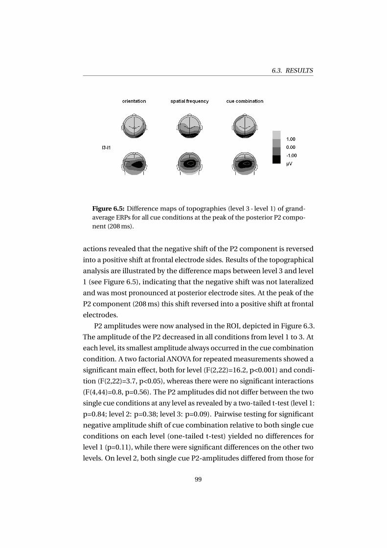
6.3. RESULTS
Figure 6.5: Difference maps of topographies (level 3 - level 1) of grand-average ERPs for all cue conditions at the peak of the posterior P2 compo-nent (208ms).
actions revealed that the negative shift of the P2 component is reversed
into a positive shift at frontal electrode sides. Results of the topographical
analysis are illustrated by the difference maps between level 3 and level
1 (see Figure 6.5), indicating that the negative shift was not lateralized
and was most pronounced at posterior electrode sites. At the peak of the
P2 component (208ms) this shift reversed into a positive shift at frontal
electrodes.
P2 amplitudes were now analysed in the ROI, depicted in Figure 6.3.
The amplitude of the P2 decreased in all conditions from level 1 to 3. At
each level, its smallest amplitude always occurred in the cue combination
condition. A two factorial ANOVA for repeatedmeasurements showed a
significant main effect, both for level (F(2,22)=16.2, p<0.001) and condi-
tion (F(2,22)=3.7, p<0.05), whereas there were no significant interactions
(F(4,44)=0.8, p=0.56). The P2 amplitudes did not differ between the two
single cue conditions at any level as revealed by a two-tailed t-test (level 1:
p=0.84; level 2: p=0.38; level 3: p=0.09). Pairwise testing for significant
negative amplitude shift of cue combination relative to both single cue
conditions on each level (one-tailed t-test) yielded no differences for
level 1 (p=0.11), while there were significant differences on the other two
levels. On level 2, both single cue P2-amplitudes differed from those for
99
KAPITEL 6. SALIENCY-ERP & IDENTIFICATION TASK
cue combination (p<0.05). Whereas this also held for the comparison
between the orientation and the cue combination condition on level 3
(p<0.05), the difference between spatial frequency and cue combination
conditions did not reach statistical significance (p=0.08). This hetero-
geneity of results was due to a large diversity in P2-amplitudes across
subjects (see amplitude standard errors in Figure 6.6A). In the further
analysis we dealt with this fact by using an amplitude normalization
technique.
Relationship betweenP2-component and saliency. Subjects’ performance
increased monotonically with increasing object saliency. This fact makes
performance a direct indicator for saliency, irrespective of the underlying
cue configuration. The behavioural data (Figure 6.2) show that all subjects
benefited perceptually in the cue combination condition (as indicated by
better performance). Hence, within a given level, the cue combination
condition differed not only in its physical parameters (two cues), but
also in its saliency. Is the observed effect at the posterior P2 component
primarily related the physical stimulus properties or else to perceived
saliency?
To disclose the nature of the reduction in P2-amplitude, we re-exam-
ined the individual P2-amplitude changes in relation to individual per-
formance in each particular experimental configuration (cue condition
and level). The amplitude change was defined as the deviation from the
individual mean (composed of all nine individual P2-amplitude mea-
surements) and correlated with the individually measured d’ value as a
performance measure. Figure 6.6B illustrates the significant correlation
between amplitude reduction of the P2 component and increasing object
saliency (correlation coefficient -0.42, p<0.001), revealing that a smaller
P2 amplitude represents an increase in perceptual saliency.
Amplitudes and latencies of the P3 component. We also observed an ef-
fect of level and cue condition on the P3 component at parietal, parieto-
occipital and occipital electrodes and evaluated these differenceswith the
samemethod and ROI as was used in the analysis of the P2 component
100
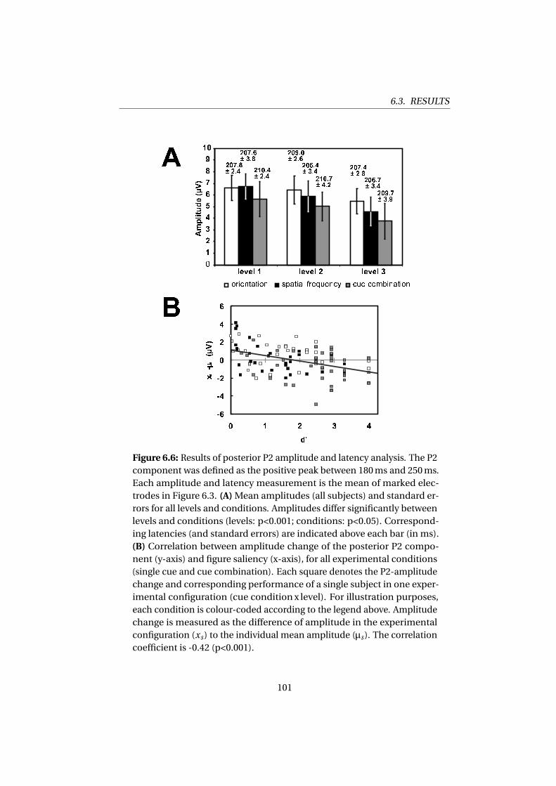
6.3. RESULTS
Figure 6.6: Results of posterior P2 amplitude and latency analysis. The P2component was defined as the positive peak between 180ms and 250ms.Each amplitude and latency measurement is the mean of marked elec-trodes in Figure 6.3. (A)Mean amplitudes (all subjects) and standard er-rors for all levels and conditions. Amplitudes differ significantly betweenlevels and conditions (levels: p<0.001; conditions: p<0.05). Correspond-ing latencies (and standard errors) are indicated above each bar (in ms).(B) Correlation between amplitude change of the posterior P2 compo-nent (y-axis) and figure saliency (x-axis), for all experimental conditions(single cue and cue combination). Each square denotes the P2-amplitudechange and corresponding performance of a single subject in one exper-imental configuration (cue condition x level). For illustration purposes,each condition is colour-coded according to the legend above. Amplitudechange is measured as the difference of amplitude in the experimentalconfiguration (xs) to the individual mean amplitude (μs). The correlationcoefficient is -0.42 (p<0.001).
101
KAPITEL 6. SALIENCY-ERP & IDENTIFICATION TASK
(see above and Figure 6.3). The P3 component was defined as the positive
peak in a time window between 300ms and 500ms. It had a mean am-
plitude of 7.0μV (sd 3.3μV) and a mean latency of 375.5ms (sd 38.0ms).
A two factorial ANOVA for repeatedmeasurements showed nomain ef-
fect for condition (amplitude: F(2,22)=0.5, p=0.62; latency: F(2,22)=1.1,
p=0.36), but a significant main effect for level regarding both amplitude
(F(2,22)=4.0, p<0.05) and latency (F(2,22)=11.1, p<0.001). Additionally,
the amplitude was modulated by an interaction between condition and
level (F(4,44)=4.0, p<0.01), while the latency was not (F(4,44)=1.1, p=0.36).
The P3 component varied both in amplitude and latency across experi-
mental configurations. The results imply that this modulation is mainly
based on saliency level, while the influence of the cue conditions is rather
limited. To evaluate the relation between the amplitude of the P3 compo-
nent and the saliency of the object, we correlated its amplitude changes
with the results of the behavioural analysis using the same method as
applied for the P2 component (see above and Figure 6.6B). There was no
significant correlation (see Discussion). In contrast, the peak of the P3 oc-
curred significantly later with increasing saliency (correlation coefficient
0.45, p<0.001).
Time-frequencyanalysis. Generally, we found apower increase in a broad
frequency range up to 50Hz after stimulus onset, most prominent at oc-
cipital and parieto-occiptal electrodes, with maximum activity at Oz.
Power changes at central and frontal electrodes were relatively small. We
observed no significant power reduction compared to the pre-stimulus
period. The averaged power of normalized single-subject data (see Ma-
terials andMethods) is illustrated in Figure 6.7 for all experimental con-
figurations (condition x level) at electrode Oz. This figure demonstrates
highly similar power progressions across cue conditions or performance
levels at all frequencies.
The Oz-electrode, where the power increases were most pronounced,
served as basis for our analysis. Here, we evaluated the peak of the power
increase in each frequency band (for definitions see Herrmann et al.,
2005) after stimulus onset across the whole epoch in the normalized
102
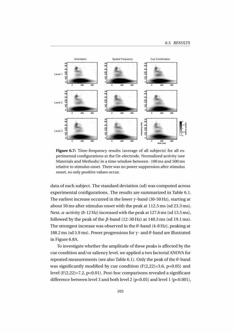
6.3. RESULTS
0 200 400
70 50
30 20 15 10 8
50 200 400
70 50
30 20 15 10 8
50 200 400
70 50
30 20 15 10 8
5
0 200 400
70 50
30 20 15 10 8
50 200 400
70 50
30 20 15 10 8
50 200 400
70 50
30 20 15 10 8
5
0 200 400
70 50
30 20 15 10 8
50 200 400
70 50
30 20 15 10 8
5
time (ms)fr
eque
ncy
(Hz)
0 200 400
70 50
30 20 15 10 8
5
rela
tive
pow
er
0
0.5
1
1.5
2
Orientation Spatial Frequency Cue Combination
Level 1
Level 2
Level 3
Figure 6.7: Time-frequency results (average of all subjects) for all ex-perimental configurations at the Oz-electrode. Normalized activity (seeMaterials andMethods) in a time window between -100ms and 500msrelative to stimulus onset. There was no power suppression after stimulusonset, so only positive values occur.
data of each subject. The standard deviation (sd) was computed across
experimental configurations. The results are summarized in Table 6.1.
The earliest increase occurred in the lower γ-band (30-50Hz), starting at
about 50ms after stimulus onset with the peak at 112.5ms (sd 23.3ms).
Next,α-activity (8-12Hz) increasedwith the peak at 127.6ms (sd 13.5ms),
followed by the peak of the β-band (12-30Hz) at 140.3ms (sd 19.1ms).
The strongest increase was observed in the θ-band (4-8Hz), peaking at
188.2ms (sd 5.9 ms). Power progressions for γ- and θ-band are illustrated
in Figure 6.8A.
To investigate whether the amplitude of these peaks is affected by the
cue condition and/or saliency level, we applied a two factorial ANOVA for
repeated measurements (see also Table 6.1). Only the peak of the θ-band
was significantly modified by cue condition (F(2,22)=3.6, p<0.05) and
level (F(2,22)=7.2, p<0.01). Post-hoc comparisons revealed a significant
difference between level 3 and both level 2 (p<0.05) and level 1 (p<0.001),
103
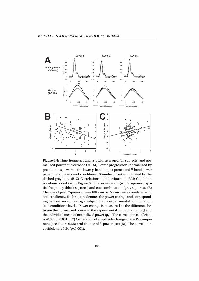
KAPITEL 6. SALIENCY-ERP & IDENTIFICATION TASK
0 200 400
ms
rela
tive
po
wer
0 200 400 0 200 400
0 200 4000
1
2
3
ms
rela
tive
po
wer
0 200 4000
1
2
3
0 200 4000
1
2
3
0
-0.2
0.2
0.4
0.6
0.8
0
-0.2
0.2
0.4
0.6
0.8
0
-0.2
0.2
0.4
0.6
0.8
orientation spatial frequency cue combination
Level 1 Level 2 Level 3
lower -band
(30-50 Hz)
�
�-band
(4-8 Hz)
A
B C
-1
1
0 1 2 3 4
d'
ch
an
ge
of
po
wer
-6
-4
-2
0
2
4
6
-2 -1 0 1 2
change of power
ch
an
ge
of
P2
(μV
)
Figure 6.8: Time-frequency analysis with averaged (all subjects) and nor-malized power at electrode Oz. (A) Power progression (normalized bypre-stimulus power) in the lower γ-band (upper panel) and θ-band (lowerpanel) for all levels and conditions. Stimulus onset is indicated by thedashed grey line. (B-C) Correlations to behaviour and ERP. Conditionis colour-coded (as in Figure 6.6) for orientation (white squares), spa-tial frequency (black squares) and cue combination (grey squares). (B)Changes of peak θ-power (mean 188.2ms, sd 5.9ms) were correlated withobject saliency. Each square denotes the power change and correspond-ing performance of a single subject in one experimental configuration(cue condition x level). Power change is measured as the difference be-tween the normalized power in the experimental configuration (xs) andthe individual mean of normalized power (μs). The correlation coefficientis -0.38 (p<0.001). (C) Correlation of amplitude change of the P2 compo-nent (see Figure 6.6B) and change of θ-power (see (B)). The correlationcoefficient is 0.34 (p<0.001).
104
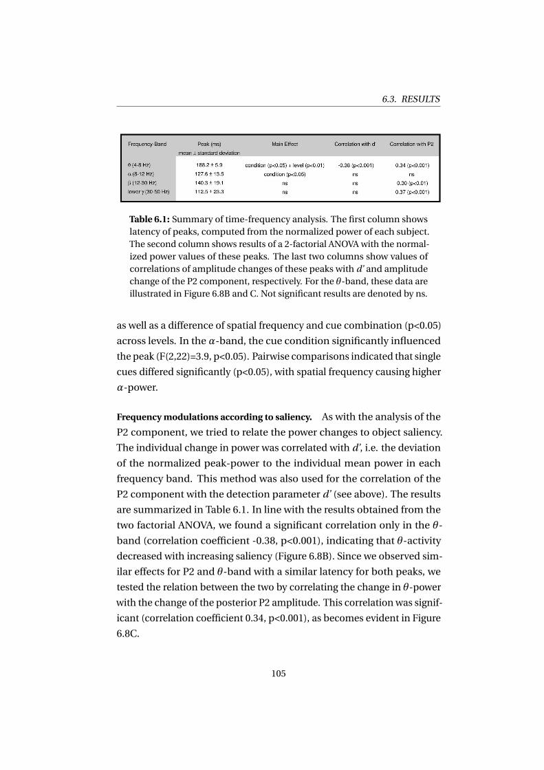
6.3. RESULTS
Table 6.1: Summary of time-frequency analysis. The first column showslatency of peaks, computed from the normalized power of each subject.The second column shows results of a 2-factorial ANOVA with the normal-ized power values of these peaks. The last two columns show values ofcorrelations of amplitude changes of these peaks with d’ and amplitudechange of the P2 component, respectively. For the θ-band, these data areillustrated in Figure 6.8B and C. Not significant results are denoted by ns.
as well as a difference of spatial frequency and cue combination (p<0.05)
across levels. In the α-band, the cue condition significantly influenced
the peak (F(2,22)=3.9, p<0.05). Pairwise comparisons indicated that single
cues differed significantly (p<0.05), with spatial frequency causing higher
α-power.
Frequencymodulations according to saliency. As with the analysis of the
P2 component, we tried to relate the power changes to object saliency.
The individual change in power was correlated with d’, i.e. the deviation
of the normalized peak-power to the individual mean power in each
frequency band. This method was also used for the correlation of the
P2 component with the detection parameter d’ (see above). The results
are summarized in Table 6.1. In line with the results obtained from the
two factorial ANOVA, we found a significant correlation only in the θ-
band (correlation coefficient -0.38, p<0.001), indicating that θ-activity
decreased with increasing saliency (Figure 6.8B). Since we observed sim-
ilar effects for P2 and θ-band with a similar latency for both peaks, we
tested the relation between the two by correlating the change in θ-power
with the change of the posterior P2 amplitude. This correlation was signif-
icant (correlation coefficient 0.34, p<0.001), as becomes evident in Figure
6.8C.
105
KAPITEL 6. SALIENCY-ERP & IDENTIFICATION TASK
Surprisingly, we also observed such a significant correlation for the
β- (correlation coefficient 0.30, p<0.01) and lower γ-bands (correlation
coefficient 0.37, p<0.001), although the corresponding peaks occurred
much earlier and we found no effect of cue condition or saliency onto
these peaks (see also Table 6.1).
6.4 Discussion
A definition of an object by cue combination improves its identification
by the visual system. At least for spatial frequency and orientation this
improvement is synergistic. Both behavioural and electrophysiological
results imply that the visual system uses both cues for the recognition
process. The first correlates of this process are observed as a negative
amplitude shift, influencing mainly the peak amplitude of the poste-
rior P2 component at about 200ms. We demonstrated that this shift is
strongly correlated to the perceived saliency of the figure and therefore
only indirectly related to the underlying physical cue configuration. The
same effect can be demonstrated by a relative power decrease of the
θ-band. In the following, we integrate the findings of our study in the
present literature and further discuss the relationship between saliency
and the underlying physical figure-ground differences, as well as the ob-
served P2 effect. Finally, we briefly deal with the changes of the P3, whose
characteristics slightly change near perceptual threshold.
Synergy through combination of cues. Our results confirm that the com-
bination of spatial frequency and orientation improves the identification
of a figure, exceeding the predictions of an independent summation
assumption (Meinhardt & Persike, 2003; Meinhardt et al., 2004, 2006;
Persike &Meinhardt, 2006). This result was obtained, although subjects
trained the single cue conditions (during QUEST andMCSmeasures) and
were first confronted with the cue combination in the main experiment,
indicating that the strong perceptual benefit of cue combination is a very
robust and reliable effect.
106
6.4. DISCUSSION
The electrophysiological data showmarked changes for cue combi-
nation even on level 3, where behavioural improvement was limited due
to ceiling effects, indicating that ERPs reflect easier recognition even
for perfect performance. The main finding is an early ERP modulation
that is linearly related to object saliency, which in turn is based on all
cues. Therefore, the process of cue combination occurs before or during
the segregation of the figure. Visual cues like orientation and spatial
frequency are detected in the primary visual cortex (V1), while the pro-
cessing of cue differences requires interactions between the detectors
for figure and background regions. The earliest intermediate area, inte-
grating information from V1, is area V2, which seems to be anatomically
and functionally ideally suited for segregation processes (Shipp & Zeki,
2002a,b). Computational models of texture segregation have demon-
strated that the actual segregation process is accomplished by feedback
from higher onto early visual areas (Bullier, 2001; Deco & Rolls, 2004;
Itti & Koch, 2001; Roelfsema et al., 2002; Zwickel et al., 2007) and there-
fore occurs later in time. Saliency, which is a rather perceptual object
property, is certainly related to these reactivations of early visual areas
by top-down control. Indeed, it has been shown that an early negative
shift in the ERP during the processing of illusory contours was caused by
the lateral-occipital complex (LOC) or at least modulated via feedback
from the LOC (Murray et al., 2002, 2004), a region which is known to be
involved in object recognition. Also the later negativity associated with
closure has been attributed to LOC (Doniger et al., 2000, 2001; Sehatpour
et al., 2006).
Saliency as a non-linear function of physical figure-ground difference. The
earliest electrophysiological difference between both performance levels
and cue conditions is an amplitude change of the posterior P2-amplitude.
Unfortunately, there are only a few studies that observe a posterior P2,
since N1, N2 and P3 components are often overlapping (Luck, 2005,
Chapter 1). The present study shows that the amplitude change of the
P2 represents a change in perceptual saliency rather than directly rep-
resenting the physical properties of the stimulus. Saliency is of course
107
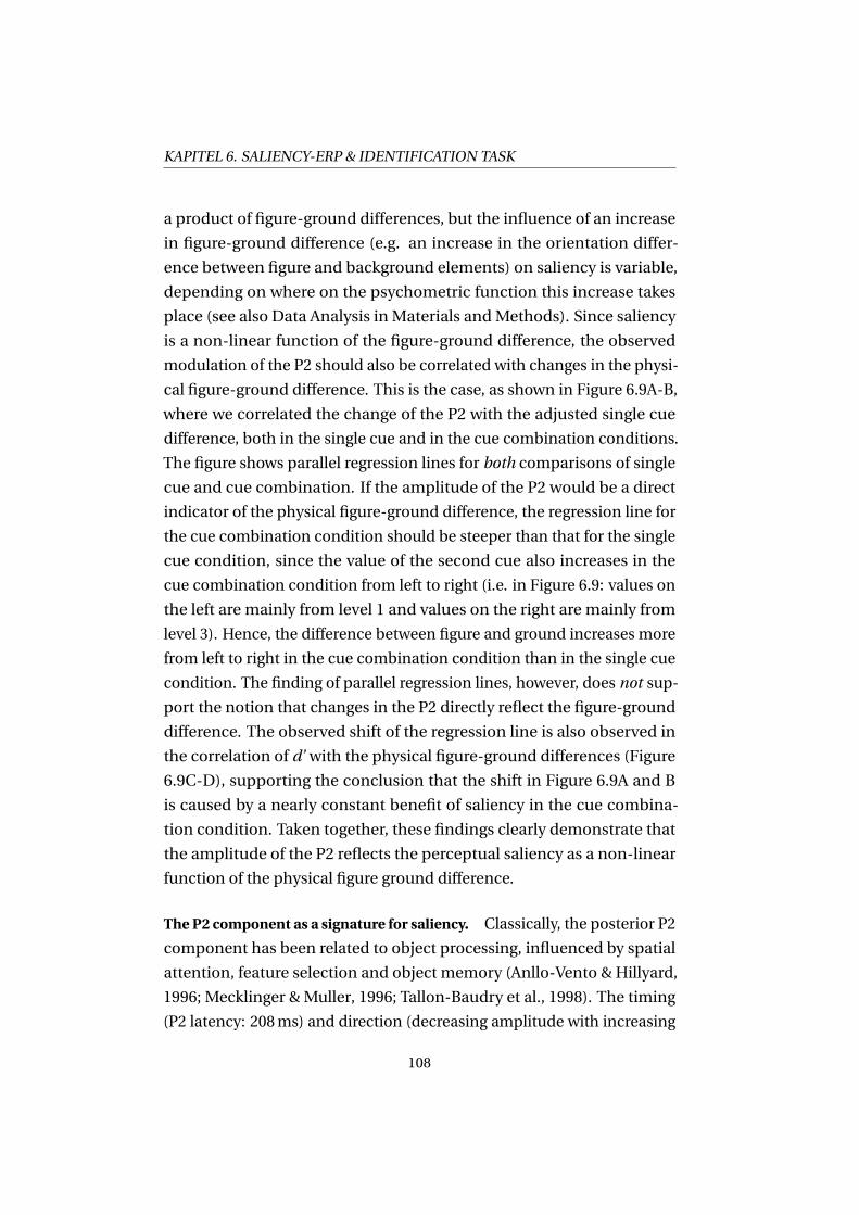
KAPITEL 6. SALIENCY-ERP & IDENTIFICATION TASK
a product of figure-ground differences, but the influence of an increase
in figure-ground difference (e.g. an increase in the orientation differ-
ence between figure and background elements) on saliency is variable,
depending on where on the psychometric function this increase takes
place (see also Data Analysis inMaterials andMethods). Since saliency
is a non-linear function of the figure-ground difference, the observed
modulation of the P2 should also be correlated with changes in the physi-
cal figure-ground difference. This is the case, as shown in Figure 6.9A-B,
where we correlated the change of the P2 with the adjusted single cue
difference, both in the single cue and in the cue combination conditions.
The figure shows parallel regression lines for both comparisons of single
cue and cue combination. If the amplitude of the P2 would be a direct
indicator of the physical figure-ground difference, the regression line for
the cue combination condition should be steeper than that for the single
cue condition, since the value of the second cue also increases in the
cue combination condition from left to right (i.e. in Figure 6.9: values on
the left are mainly from level 1 and values on the right are mainly from
level 3). Hence, the difference between figure and ground increases more
from left to right in the cue combination condition than in the single cue
condition. The finding of parallel regression lines, however, does not sup-
port the notion that changes in the P2 directly reflect the figure-ground
difference. The observed shift of the regression line is also observed in
the correlation of d’ with the physical figure-ground differences (Figure
6.9C-D), supporting the conclusion that the shift in Figure 6.9A and B
is caused by a nearly constant benefit of saliency in the cue combina-
tion condition. Taken together, these findings clearly demonstrate that
the amplitude of the P2 reflects the perceptual saliency as a non-linear
function of the physical figure ground difference.
The P2 component as a signature for saliency. Classically, the posterior P2
component has been related to object processing, influenced by spatial
attention, feature selection and object memory (Anllo-Vento & Hillyard,
1996; Mecklinger &Muller, 1996; Tallon-Baudry et al., 1998). The timing
(P2 latency: 208ms) and direction (decreasing amplitude with increasing
108
6.4. DISCUSSION
x-μ
(μV
)s
s
-6
-4
-2
0
2
4
6
A B
0 5 10 15 20 25 30
Difference to Background (°)
C
-2
0
2
4
6
d’
'
0 0.5 1.0 1.5 2.0
Difference to Background (cpd)
D
Figure 6.9: Electrophysiological and behavioural changes with increasingfigure-ground differences. (A-B) Correlation between amplitude changeof the P2 component and figure-ground difference in the stimulus forsingle and combined cues. (A) Orientation cue in black (correlation coef-ficient -0.38; p<0.05) and cue combination in grey (correlation coefficient-0.30; p=0.07). (B) Spatial frequency cue in black (correlation coefficient-0.54; p<0.01) and cue combination in grey (correlation coefficient -0.55;p<0.001). (C-D) Correlation between saliency (d’) and figure-ground dif-ference in the stimulus for single and combined cues. (C)Orientation cuein black (correlation coefficient 0.68; p<0.001) and cue combination ingrey (correlation coefficient 0.69; p<0.001). (D) Spatial frequency cue inblack (correlation coefficient 0.70; p<0.001) and cue combination in grey(correlation coefficient 0.65; p<0.001).
109
KAPITEL 6. SALIENCY-ERP & IDENTIFICATION TASK
saliency) of the P2 differences we find are in line with previous studies
reporting a segregation-specific negative amplitude shift between 100ms
and 300ms (Bach &Meigen, 1992, 1997; Bach et al., 2000; Caputo & Casco,
1999; Fahle et al., 2003; Mathes et al., 2006; Mathes & Fahle, 2007). The
present findings extend these results by indicating that the negative shift
is not only segregation-specific, but at some point in time directly corre-
lated with perceptual saliency. In an overview article, Bach andMeigen
(1998) reported a correlation between the tsVEP and saliency, when they
increased saliency by changing the line length of a checkerboard stimulus.
In their report, the normal VEP did not show a consistent modulation as
a result of varying saliency, while the amplitude of the tsVEP increased.
Here, we substantiate their conclusion by measuring individual salien-
cies and by systematically varying figure-ground difference and cue. The
saliency-effect we find in the ERP ismostly unaffected by the number and
type of cues. Contrary to Bach and Meigen, we observe a strong effect on
the normal ERP (i.e. a modulation of the P2 component) which is blurred
in the difference-ERPs (compare Figure 6.4). Even when task and stimu-
lus were slightly changed, as in the control experiment, we observed the
occurrence of a P2 component which was diminished when the figure
was present in the stimulus. The task in this control was much simpler,
since only detection (yes/no) of the figure was necessary while recogni-
tion was not mandatory. Therefore, the task was easier to accomplish,
so the task-related saliency was even higher than the adjusted level 3
of the identification experiment. This observation suggests that the P2
effect found in this study is task independent and exclusively related to
saliency. We therefore propose that amplitude changes of the posterior
P2 component generally indicate changing saliency.
Our findings support theories of a common saliency map, which is
created by the combined responses of selectively modulated neurons (for
a review see Treue, 2003). The P2 modulation we observed could well be
a correlate of this saliency representation, since it is mainly affected by
saliency irrespective of cue condition.
110
6.4. DISCUSSION
Butwhy doweobserve an amplitude reduction of the P2when saliency
increases? If the amplitude decrease is interpreted as less neural activ-
ity, one possible explanation would be that the processes involved are
mediated by attention. Global attentional effects were controlled in our
experiment by pseudorandomizing stimulus levels within conditions and
order of blocks between subjects. However, selective attention might
mediate enhanced population activity in order to improve the perfor-
mance for weakly salient stimuli (Maunsell & Treue, 2006; Treue, 2003),
whereas highly salient stimuli needed little or no attentional allocation
in psychophysical tasks (see e.g. Nothdurft, 2000). Then the decrease of
attentional allocation required to solve the task would be inversely pro-
portional to figure saliency, which is exactly what we observe. Consistent
with this view a recent study observed a similar effect on the posterior
P2 component in a masking paradigm (Kotsoni et al., 2007), the ampli-
tude of the posterior P2 also decreasing with increasing d’. The authors
interpret the P2 as a reactivation of primary and secondary visual areas
by feedback from higher areas subserving appropriate representation
of the stimulus. While not specifically quantifying the relationship to d’,
they suggest that an amplitude reduction represents a higher congruence
between bottom-up and top-down signals and therefore less interference
through feedback.
Another indirect support for our findings is given by a study, reporting
a temporal blurring of the posterior P2 with increasing eccentricity (Shoji
& Ozaki, 2006). Here, the saliency of the target (a circle) depended on
the distractor type (squares, hexagons or octagons) and the P2 amplitude
also declined with increasing saliency.
Relation of θ-power to ERP and saliency. We found the earliest increase
of energy in the lower γ-band around 40Hz, a well known phenomenon
in object detection and discrimination tasks (Busch et al., 2004, 2006;
Senkowski & Herrmann, 2002). Yet, this energy was stable across ex-
perimental conditions, so we conclude that the early onset γ-activity
is not specific to the visual cues modified here and neither to object
saliency. Later activations in the γ-band (e.g. induced γ-activity) were
111
KAPITEL 6. SALIENCY-ERP & IDENTIFICATION TASK
not observed in our paradigm. It has been suggested that induced γ-band
activity is a candidate for active binding of visual features (Tallon-Baudry
& Bertrand, 1999). However, this does not seem to be the case for simple
visual cues such as orientation and spatial frequency.
At lower frequencies, we observed amodulation of the θ-band (4-8Hz).
Functionally, θ is related to short termmemory and selective attention
(Basar et al., 1999), whereas it is unlikely that it has a single functional
role (Kahana et al., 2001). In our study, θ-activity decreased with increas-
ing saliency at a latency around 188ms. The maximum of θ-activity
is near the peak of the P2 component, which in turn has a strong θ-
component, suggesting that both strongly depend on each other. Ac-
cordingly, a wavelet transformation of the ERP shows a strong θ-peak
at a latency near the P2, indicating that most of the θ-activity is time
locked and therefore shows up in the ERP. However, the temporal reso-
lution of the wavelet analysis is very poor at these low frequencies, and
we could, nevertheless, clearly demonstrate that the effect of increased
cue-independent saliency is related to a reduction in the θ-band.
Moreover, we found significant correlations of activity changes at
other frequency bands with changes of the P2 even at earlier latencies
(compare Table 6.1), although these were unrelated to saliency. These
changes could probably be a hint of how the P2 component is generated,
but this issue should be a subject of future studies.
The P3 component. The P3 represents a major endogenous component,
which is moreover influenced by a number of experimental parameters
(Fabiani et al., 2000; Key et al., 2005; Luck, 2005, Chapter 1). In our study,
the amplitude and latency of the P3 were influenced mainly by perfor-
mance levels, which affect many endogenous parameters (in addition to
exogenous ones), for example by making subjects less confident about
their decision, rendering the task more difficult, requiring longer process-
ing and increasing the proportion of guesses.
Classically, the amplitude of the P3 component has been related to
working memory update (Polich & Kok, 1995; Polich, 2004), although
such update processes seem not mandatory (Picton, 1992). The P3 ampli-
112
6.5. CONCLUSIONS
tude decreases while its latency increases when the task becomes more
difficult, indicating that the P3 is involved in stimulus classification and
decision making processes (Picton, 1992; Polich & Kok, 1995). Although
the ANOVA showed a significant effect of performance level on the P3 am-
plitude, the correlation of P3 amplitude with saliency was not significant,
possibly because a large proportion of trials was near or below perceptual
threshold (d’=1.0) and might have been correctly guessed while not really
recognized. In other words, below perceptual threshold the fraction of
really recognized figures is small compared to the correctly guessed trials
(50 percent correct). Excluding all trials with d’<1.0 and correlating the
remaining trials with the P3 amplitude observed yielded indeed a signifi-
cant correlation between amplitude and saliency (correlation coefficient
0.26, p<0.05). Hence, the classical relationship of increasing P3 amplitude
with decreasing task difficulty holds at least above perceptual threshold.
The latency of the P3 has been attributed to stimulus classification
and processing (Polich & Kok, 1995; Polich, 2004), with longer latencies
occurring in more difficult trials. Quite contrary, we observe longer la-
tencies with easier trials. In contrast to classical studies investigating
the P3, our target is hardly visible even on the easiest performance level.
Visual noise distorts the P3 (McCarthy & Donchin, 1981), so the trend
we observe here may reflect the emergence of the P3 out of noise with
higher saliencies. Our results imply that the characteristics of the P3 near
perceptual threshold have to be reviewed.
6.5 Conclusions
Orientation and spatial frequency interact as visual cues during the iden-
tification of a figure. This interaction, based on cue combination, is
neither specifically reflected in the ERP nor in the power distribution
of frequencies up to 80Hz. Instead, the crucial feature of the neural re-
sponse is a negative shift in the ERP, which occurs on an intermediate
stage (about 200ms after stimulus onset) correlated to saliency. This shift
is measurable as an amplitude modulation of the posterior P2 compo-
nent as well as a power reduction in the θ-band (4-8Hz). A posterior P2
113
KAPITEL 6. SALIENCY-ERP & IDENTIFICATION TASK
component is rarely described in the literature which may be based on
the fact that other studies used highly salient stimuli. With the present
work, we explored the direct relationship between the P2 amplitude and
object saliency, probably reflecting the existence of a cue independent
saliency map and/or reflecting the fact that the more salient an object
is, the less computation is required to detect or identify it. This saliency
effect on the ERP is robust across different cues and number of cues,
maybe even across tasks, and should be considered in future studies as
an important factor affecting the results. Furthermore, our study pro-
vides the basis for the development of an electrophysiological method
to evaluate the strength of perceptual impressions in humans, either by
utilising the negative shift of the ERP (in particular the P2 component) or
the power decrease of the θ-band.
Acknowledgements
The authors like to thank B. Mathes, D. Trenner, U. Ernst and G. Mein-
hardt for valuable suggestions. Supported by grant 01GQ0705 (Bernstein
programme) of the German Federal Ministry of Education and Research
(BMBF).
114
Kapitel 7
Visual detection and
identification are not the same:
evidence from psychophysics
and fMRI
Sirko Straube &Manfred Fahle
Abstract
The remarkable speed of human categorization performance in natural
scenes led to the assumption that detection and identification processes
rely on the same mechanism (Grill-Spector & Kanwisher, 2005). In the
present study we test this assumption by combining psychophysical
measurements and functional magnetic resonance imaging (fMRI) for
both a detection and an identification task. A target was embedded in
a matrix of Gabor elements with its elements differing from the back-
ground ones in their orientation. We yielded equal performance levels for
detection and identification bymeasuring the individual psychometric
functions and adjusting orientation differences accordingly for each ob-
115
KAPITEL 7. DETECTION VERSUS IDENTIFICATION
server. Hence, stimulus saliency was constant allowing a differentiation
between the activations specific for detection versus identification pro-
cesses. There were three task conditions: (i) figure detection (left/right;
based on small orientation differences), (ii) figure identification (sym-
metrical/asymmetrical; requiring larger orientation differences) and (iii)
detection of a scrambled figure (left/right; using the larger orientation dif-
ferences of the identification task). Identification led to higher thresholds
on the psychometric functions and to slower reaction times than detec-
tion. The fMRI data showed increased hemodynamic activations during
the identification task in subdivisions of the lateral-occipital complex
(LOC) and in a neighbouring area in the collateral sulcus. In addition,
analysis using cortex-based alignment revealed four voxel-clusters dif-
ferently activated by the tasks, situated in the inferior parietal lobe, the
precuneus, the anterior cingulum and the medial frontal gyrus. Our re-
sults indicate at least partly separated cortical mechanisms for object
detection and identification.
7.1 Introduction
Visual perception of an object is instantly connected with an idea of
what we see and usually this first impression is correct. Nevertheless,
sometimes we fail and sometimes we just have the impression that there
was something. Our visual system permanently trades off between speed
and accuracy, allowing us to react fast to a snake hidden in the woods and
at the same time preventing us from reacting to every stick thatmight
be a snake. Hence, the detection and the identification of an object are
closely related, one influencing the other (Peterson & Gibson, 1994), and
it is an old questionwhether detection and identification rely on the same
mechanism operating with different outcomes depending on stimulus
strength and task demand, or on at least partly separate mechanisms
operating with different time constants. In the early 1980s, Sagi and
Julesz (1984) characterized detection as a preattentive, parallel process as
opposed to identification as a serial process requiring attention. Since
116
7.1. INTRODUCTION
both processes have different characteristics, it has been suggested they
rely on at least partly different mechanisms.
Nowadays this dichotomy is not so clear anymore. Two behavioural
studies draw opposite conclusions when using backward masking of nat-
ural scenes. They compared the stimulus-onset asynchrony thresholds
of detection, basic-level categorization and within-category identifica-
tion (Grill-Spector & Kanwisher, 2005; Mack et al., 2008). Grill-Spector
and Kanwisher (2005) claim in the title of their article that “As soon as
you know it is there, you know what it is”, implying that detection and
identification of objects in complex scenes are inseparable. Functional
magnetic resonance imaging (fMRI) studies only compared detection and
within-category identification (and not basic-level categorization), also
concluding that detection and recognition are inseparable (Grill-Spector,
2003a; Grill-Spector et al., 2004). On the other hand, Mack and colleagues
(2008) demonstrated that additional stimulus manipulations reducing
object saliency can indeed result in dissociation between detection and
identification. Hence, detecting an object does not necessarily mean to
know what that object is.
In these studies, the term identification is used for discrimination
within a category, which differs clearly from the definition of Sagi and
Julesz (see above) who associate identification more with recognition.
When they refer to recognition, Grill-Spector and Kanwisher use the term
basic-level categorization. In the following, we will follow the nomencla-
ture of Sagi and Julesz and speak of detection, identification (in the sense
of recognition) and within-category identification (i.e. discrimination
within a category).
An fMRI study directly comparing detection and identification (in
the sense of recognition) is still lacking. Our study is a first step in this
direction where we used a novel approach to successfully separate the
two processes. Although our stimulus differs from that of Mack and col-
leagues, the basic idea for dissociating both tasks is similar: detection
does not require global shape perception, so it can be achieved based
on local differences in the stimulus. Therefore, it is crucial to carefully
117
KAPITEL 7. DETECTION VERSUS IDENTIFICATION
control the saliency of the target. The perceived saliency of an object at
detection threshold differs from the saliency of that same object when
it should be identified: As mentioned above, sometimes wemay detect
a snake in the woods without recognizing it. Here, we create a similar
situation by individually adjusting the physical figure-ground difference
according to task demands based on the percept of each individual sub-
ject. We then investigated whether the different tasks of detection versus
identification at identical saliency caused different blood oxygenation
level-dependent (BOLD) responses in visual and object-selective areas,
which were functionally mapped in a separate session. Additionally, we
applied a cortex-based alignment procedure to find further differences
in the processing of these tasks across the whole brain.
Three tasks had to be performed: (i) detection of the figure, i.e. to
indicate whether the figure was left or right, (ii) identification of the
figure, i.e. to indicate whether it was symmetrical or asymmetrical, and
(iii) detection of a scrambled figure, i.e. to indicate whether it was left or
right. The third condition served to control for the effect possibly caused
purely by variation of the figure-ground difference due to the fact that this
difference is larger in the identification task than in the detection task.
This scrambled-figure condition was a detection task, where the target
exhibits the figure-ground difference of the identification task. Here,
performance was varied by distributing the target elements across the
whole area where the figure could appear in the other two tasks. Hence,
subjects had to detect the side with more target elements (left or right).
With this design we kept the target saliency constant and thereby sep-
arated detection and identification processes, while making sure that all
tasks yielded the same level of performance. Differences in behavioural
measurements and/or in BOLD activations would indicate that detection
and identification are at least partly differentially processed, suggesting
that also partly separated mechanisms operate. For neural activations
in the visual system, this could mean that the two tasks do not activate
exactly the same areas. For example, as argued above, shape perception
118
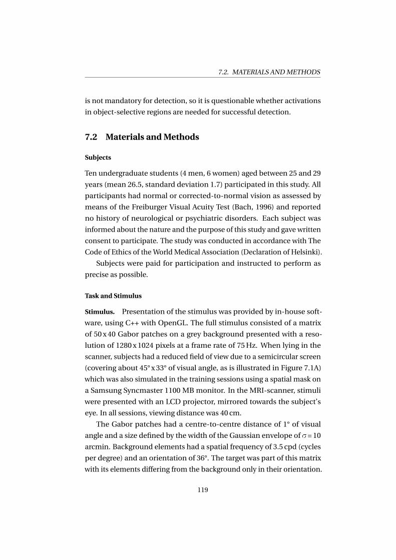
7.2. MATERIALS AND METHODS
is not mandatory for detection, so it is questionable whether activations
in object-selective regions are needed for successful detection.
7.2 Materials andMethods
Subjects
Ten undergraduate students (4 men, 6 women) aged between 25 and 29
years (mean 26.5, standard deviation 1.7) participated in this study. All
participants had normal or corrected-to-normal vision as assessed by
means of the Freiburger Visual Acuity Test (Bach, 1996) and reported
no history of neurological or psychiatric disorders. Each subject was
informed about the nature and the purpose of this study and gave written
consent to participate. The study was conducted in accordance with The
Code of Ethics of the World Medical Association (Declaration of Helsinki).
Subjects were paid for participation and instructed to perform as
precise as possible.
Task and Stimulus
Stimulus. Presentation of the stimulus was provided by in-house soft-
ware, using C++ with OpenGL. The full stimulus consisted of a matrix
of 50 x 40 Gabor patches on a grey background presented with a reso-
lution of 1280 x 1024 pixels at a frame rate of 75Hz. When lying in the
scanner, subjects had a reduced field of view due to a semicircular screen
(covering about 45° x 33° of visual angle, as is illustrated in Figure 7.1A)
which was also simulated in the training sessions using a spatial mask on
a Samsung Syncmaster 1100 MB monitor. In the MRI-scanner, stimuli
were presented with an LCD projector, mirrored towards the subject’s
eye. In all sessions, viewing distance was 40 cm.
The Gabor patches had a centre-to-centre distance of 1° of visual
angle and a size defined by the width of the Gaussian envelope of �=10
arcmin. Background elements had a spatial frequency of 3.5 cpd (cycles
per degree) and an orientation of 36°. The target was part of this matrix
with its elements differing from the background only in their orientation.
119
KAPITEL 7. DETECTION VERSUS IDENTIFICATION
Figure 7.1: Stimulus, Targets and Conditions. (A) Trial sequence (left).Stimulus was presented for 80ms on a semicircular screen. Colour of thefixation point during the fixation phase instructed the subjects which taskto perform. Answer was given after the stimulus disappeared, i.e. duringfixation phase for the next trial. The shapes of the possible figures (exceptscrambled-figure condition) are depicted on the right. Symmetrical orasymmetrical figures occurred balanced in pseudorandomized order. (B)20 x 20 elements cut-out of the original stimulus (see above) to illustrateexperimental conditions. Instruction to subjects is indicated below thestimuli. Arrows denote lower border of the target.
120
7.2. MATERIALS AND METHODS
A trial started with a fixation point in the middle of a grey background
(2000ms), followed by a short flash of the stimulus (80ms). In the subse-
quent fixation phase, subjects had to respond to the previous stimulus
by pressing one of two buttons (2-alternative forced choice). There were
three tasks and a baseline condition (see Figure 7.1B): (i) detection of a fig-
ure, (ii) identification of a figure and (iii) detection of a scrambled figure.
We calibrated the saliency of all three tasks individually for each observer
to a similar level before subjects performed the tasks pseudorandomized
in a block design (see below). The colour of the fixation point indicated
the task demand (detection or else identification). Tasks and baseline
condition are described next, the experimental procedure is illustrated
thereafter.
Figure Detection. A black fixation point instructed the subjects to indi-
cate whether the target appeared left or right of the vertical midline. A
figure (symmetrical or else asymmetrical — see Figure 7.1A) was ran-
domly rotated into one of four orientations to produce the stimulus, but
its appearance was irrelevant for the correct answer. Instead, observers
had to indicate whether its centre of gravity was left or right of themidline.
Its inner edges always intruded into the opposite half by 1° while its outer
edges were no more eccentric than 7° of visual angle.
Figure Identification. A red fixation point instructed the subjects to indi-
cate whether the target was symmetrical or asymmetrical (Figure 7.1A).
The composition of the stimuli was identical to those of the figure de-
tection task, but here subjects had to ignore the position of the figure.
To solve this task, they had to recognize nearly the whole figure, since
detection of single edges was not sufficient to discriminate between the
two figure types.
Detection of Scrambled Figure. Just like in the figure detection task, a
black fixation point instructed the subjects to indicate whether the target
appeared left or right of the midline. The stimuli of the detection and
the identification task differed between each other in two aspects: the
121
KAPITEL 7. DETECTION VERSUS IDENTIFICATION
task itself (which is the object of the current study) and the underlying
physical figure-ground difference in element orientation. To rule out
the possibility that differences in the results are attributable to the latter,
we added this third task which is a detection task without a solid figure,
where the targets’ Gabor elements have the same orientation difference
as in the identification task. Saliency was controlled by variation of the
target position over the whole visual field (see Figure 7.1B). Therefore,
both shape and target position were blurred in this task. To solve the
task, subjects again had to estimate the centre of gravity of this scrambled
figure.
BaselineCondition. This conditionwas as similar as possible to the three
tasks. The Gabor matrix contained no target and consisted only of ho-
mogenous Gabor elements identical to the background elements in the
other conditions. A white fixation point indicated the baseline condition,
and subjects were instructed to alternately press the left and right buttons
once after each stimulus in the answer/fixation phase.
Procedure
Before subjects performed the experiment in the MRI-scanner, they
trained on three days with exactly the same procedure as in the scanner.
Nomore than ten days lay between the first day of training and the final
MRI-experiment. The procedure of these experimental sessions was as
follows: First, we individually measured the turning point and slope of
the psychometric function for each task (detection, identification, scram-
bled figure detection) using a QUEST staircase procedure (Watson & Pelli,
1983) with 100 trials each. Second, the values obtained by the QUEST
measurements were used for six consecutive runs where all conditions
including the baseline condition occurred in a block design paradigm.
QUEST staircase. The psychometric function was scaled between guess-
ing probability (50%) and performance limit (100%). In the figure detec-
tion or identification conditions, the parameter varied by QUEST was the
122
7.2. MATERIALS AND METHODS
orientation difference between the figure elements and the background
elements, starting with a difference of 90°. In the scrambled figure detec-
tion task, the staircase in contrast varied the number of elements that
were presented outside the area of the original target. Here the orien-
tation difference between the target elements and the background was
adopted from the figure identification task (see description of the scram-
bled figure task). The first trial of this procedure startedwith the complete
figure.
In the training sessions auditory error feedback was provided, which
was omitted in the scanner session (day 4). The order of the staircase
measurements was pseudorandomized between sessions and subjects,
with the restriction that the identification task had to be performed before
the scrambled figure detection task, since the figure-ground difference of
the former had to be known for the latter.
Blocked Runs. After measuring the individual psychometric functions
for each task using QUEST, we calculated the differences corresponding
to a correct performance of 90%. Thus, all stimuli had the same saliency.
As indicated above (see task description) the colour of the fixation point
instructed the subjects which task to perform. During each run, each
task occurred three times (10 volumes per block) with the baseline con-
dition separating task blocks (5 volumes). The order of these tasks was
randomized. Thus, we acquired 30 volumes of each task and 50 baseline
volumes per run from each subject. Because six runs were performed, we
obtained 180 volumes of each task and 300 baseline volumes per subject
in total. At the end of each run, a feedback screen informed the subject
about his or her performance.
Mapping Experiments. In a separate scanner-session, subjects under-
went mapping experiments to functionally separate early visual and
object-selective regions for the region-of-interest analysis (ROI-analysis).
During these experiments, subjects were lying in the scanner, fixating
and attending the stimulus.
123
KAPITEL 7. DETECTION VERSUS IDENTIFICATION
Borders between early visual areas (V1, V2, V3d, V3v, V4) were drawn
using a retinotopic mapping procedure in two block-design experiments
(for a detailed description of these procedures, see Spang & Morgan,
2008): First, we mapped the representation of the vertical and horizontal
visual field meridians to delineate the borders between these areas. To
that aim, we alternately stimulated a small wedge of visual field around
the horizontal or else the vertical meridian with a cartoonmovie (6 vol-
umes each block), interrupted by the baseline condition consisting of
a blank screen with a central fixation point (8 volumes/block). We per-
formed two runs, with one run consisting of 72 volumes per condition
(horizontal versus vertical) and 32 baseline volumes. Second, inner and
outer boundaries of these areas weremapped in an additional run, where
the cartoon movie was shown in one of four rings of defined eccentricity
(rings covered eccentricities between 0.8° and 23.8°). Parameters of this
run were adopted from themeridianmapping (see above), such that each
circle was also shown for 72 volumes, interrupted by a baseline condition
with a total of 32 volumes.
Object sensitive visual areas were mapped using gray-scale images of
novel objects (sculptures) contrastedwith scrambled versions of these im-
ages. The basic procedure was adopted fromGrill-Spector and colleagues
(2000). Each stimulus condition (object versus scrambled object) was
presented for 6 stimulus blocks (5 volumes per block) with interleaved
fixation periods (3 volumes per block). The order of the two conditions
was balanced. Each of 20 images for each condition was presented for
500 ms. We conducted two runs, measuring 60 volumes per condition
and 78 baseline volumes in total.
Data Acquisition. All imaging was conducted on a 3.0 T Siemens Allegra
scanner at the University of Bremen, Germany. An echo planar imaging
sequence with gradient echo sampling (TR=2.51ms, TE=30ms) was
used to acquire the functional imaging data. Thirty-eight axial slices
(2.7mm thick with 3.00mm×3.00mm in-plane resolution), covering the
whole brain, were collected with a circular-polarized head coil. The field
of view was 19.2 cm×19.2 cm with an in-plane resolution of 64×64 pixel.
124
7.2. MATERIALS AND METHODS
Data Analysis
Behavioural data. On each experimental day, we measured the parame-
ters (turning point and slope) of the psychometric function for each task
using QUEST (see above). The orientation difference leading to a correct
performance of 90% was extracted from these functions and used for the
block designed runs. During the scanner session (day 4), we additionally
recorded the reaction times for each task with a resolution of 13ms.
fMRI data. Analysis of fMRI data was based on BrainVoyagerQXTM 1.9
software (Brain Innovation, Maastricht). Functional data were pre-proc-
essed, including slice scan time correction, headmovement correction
and removal of linear trends. No spatial filter was applied. The 2D
functional images were aligned to 3D anatomical data, transformed
to Talairach & Tournoux standard coordinates (Talairach et al., 1993).
ROI-analysis and cortex-based alignment were based on segmented,
smoothed and inflated 3D-cortical surface representations (Dale et al.,
1999; Fischl et al., 1999).
We defined the regions-of-interest for each individual subject using
the data of the mapping experiments (see above). Borders between early
visual areas (V1, V2, V3d, VP, V4) were defined by the activations elicited
by stimulation of the vertical and horizontal field meridians (for method-
ology seeWarnking et al., 2002), inner and outer boundaries were defined
with the help of the eccentricity mapping and anatomical criteria. Object-
selective areas were defined by voxels responding stronger to images
containing objects compared to scrambled images (false discovery rate:
p<0.05). For three subjects we lowered this statistical threshold here to
uncorrected p<0.05, because they had very noisy data for this experiment.
Object-selective regions in the ventral pathway were separated according
to Grill-Spector et al. (2000) into three areas (lateral occipital: LO, pos-
terior fusiform gyrus: pFs, collateral sulcus: CoS) based on anatomical
criteria and their location relative to other visual areas. LO and pFs be-
long to the lateral-occiptal complex (LOC), while CoS is an area adjacent
to the LOC. For each subject, we computed for each ROI the beta-values
125
KAPITEL 7. DETECTION VERSUS IDENTIFICATION
of the general linear model (GLM) across all conditions compared to the
baseline condition. These values were normalized to %-signal change.
Effects outside the mapped ROIs were investigated using the Cortex-
Based Alignment (CBA) procedure, implemented in BrainVoyagerTM (see
e.g. Goebel et al., 2006). Hence, for each hemisphere separately, anatomi-
cal 3D-representations of the cortical surface were inflated to a sphere
and then aligned (on the basis of the sphere) for the whole group of
subjects. This procedure reduces the noise caused by inter-individual
anatomical differences during the averaging process of the functional
data. Volume time courses of the aligned brains were then used to evalu-
ate statistically significant differences between the experimental condi-
tions using a random-effects GLM.
Statistics. Statistical analysis of behavioural results and ROI-analysis
was performed using repeated measurement ANOVAs of SPSS 16.0 (SPSS
Inc., Chicago). Wherever appropriate, p-values were adjusted by Green-
house-Geisser corrections. Post-hoc pairwise comparisons were con-
ducted by using t-tests.
Regions outside the investigated ROIs showing differences in activa-
tion after the CBA were statistically tested with the repeated measure-
ments random-effects ANCOVA of the BrainVoyagerTM software package.
7.3 Results
Psychophysics. In the figure identification task, subjects needed higher
orientation differences between figure and background elements to yield
a performance equal to that in the figure detection task. This differ-
ence was evident right from the first day of training through the final
experiment in the scanner and is illustrated by the turning points of the
psychometric function. At these points, subjects perform equally well at
75%-correct for all tasks, while the elements of the figure have different
orientation differences to the background depending on the task (see Fig-
ure 7.2A). A two factorial ANOVA for repeatedmeasurements (with factors
condition and experimental day) revealed that this difference between
126
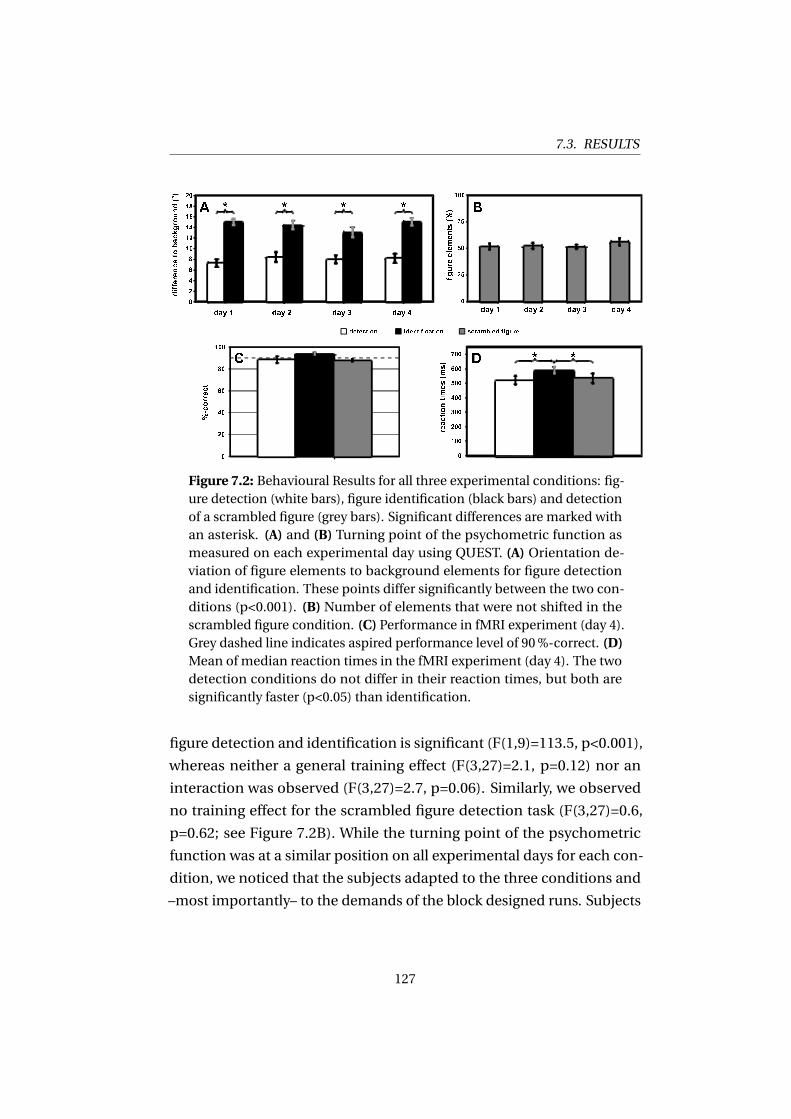
7.3. RESULTS
Figure 7.2: Behavioural Results for all three experimental conditions: fig-ure detection (white bars), figure identification (black bars) and detectionof a scrambled figure (grey bars). Significant differences are marked withan asterisk. (A) and (B) Turning point of the psychometric function asmeasured on each experimental day using QUEST. (A) Orientation de-viation of figure elements to background elements for figure detectionand identification. These points differ significantly between the two con-ditions (p<0.001). (B) Number of elements that were not shifted in thescrambled figure condition. (C) Performance in fMRI experiment (day 4).Grey dashed line indicates aspired performance level of 90%-correct. (D)Mean of median reaction times in the fMRI experiment (day 4). The twodetection conditions do not differ in their reaction times, but both aresignificantly faster (p<0.05) than identification.
figure detection and identification is significant (F(1,9)=113.5, p<0.001),
whereas neither a general training effect (F(3,27)=2.1, p=0.12) nor an
interaction was observed (F(3,27)=2.7, p=0.06). Similarly, we observed
no training effect for the scrambled figure detection task (F(3,27)=0.6,
p=0.62; see Figure 7.2B). While the turning point of the psychometric
function was at a similar position on all experimental days for each con-
dition, we noticed that the subjects adapted to the three conditions and
–most importantly– to the demands of the block designed runs. Subjects
127
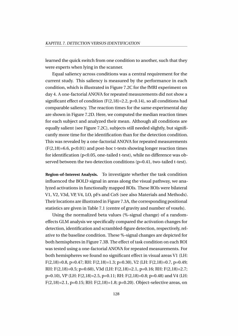
KAPITEL 7. DETECTION VERSUS IDENTIFICATION
learned the quick switch from one condition to another, such that they
were experts when lying in the scanner.
Equal saliency across conditions was a central requirement for the
current study. This saliency is measured by the performance in each
condition, which is illustrated in Figure 7.2C for the fMRI experiment on
day 4. A one-factorial ANOVA for repeated measurements did not show a
significant effect of condition (F(2,18)=2.2, p=0.14), so all conditions had
comparable saliency. The reaction times for the same experimental day
are shown in Figure 7.2D. Here, we computed the median reaction times
for each subject and analyzed their mean. Although all conditions are
equally salient (see Figure 7.2C), subjects still needed slightly, but signifi-
cantly more time for the identification than for the detection condition.
This was revealed by a one-factorial ANOVA for repeated measurements
(F(2,18)=6.6, p<0.01) and post-hoc t-tests showing longer reaction times
for identification (p<0.05, one-tailed t-test), while no difference was ob-
served between the two detection conditions (p=0.41, two-tailed t-test).
Region-of-Interest Analysis. To investigate whether the task condition
influenced the BOLD signal in areas along the visual pathway, we ana-
lyzed activations in functionally mapped ROIs. These ROIs were bilateral
V1, V2, V3d, VP, V4, LO, pFs and CoS (see also Materials and Methods).
Their locations are illustrated in Figure 7.3A, the corresponding positional
statistics are given in Table 7.1 (centre of gravity and number of voxels).
Using the normalized beta values (%-signal change) of a random-
effects GLM analysis we specifically compared the activation changes for
detection, identification and scrambled-figure detection, respectively, rel-
ative to the baseline condition. These %-signal changes are depicted for
both hemispheres in Figure 7.3B. The effect of task condition on each ROI
was tested using a one-factorial ANOVA for repeated measurements. For
both hemispheres we found no significant effect in visual areas V1 (LH:
F(2,18)=0.8, p=0.47; RH: F(2,18)=1.3; p=0.30), V2 (LH: F(2,18)=0.7, p=0.49;
RH: F(2,18)=0.5; p=0.60), V3d (LH: F(2,18)=2.1, p=0.16; RH: F(2,18)=2.7;
p=0.10), VP (LH: F(2,18)=2.5, p=0.11; RH: F(2,18)=0.8; p=0.48) and V4 (LH:
F(2,18)=2.1, p=0.15; RH: F(2,18)=1.8; p=0.20). Object-selective areas, on
128
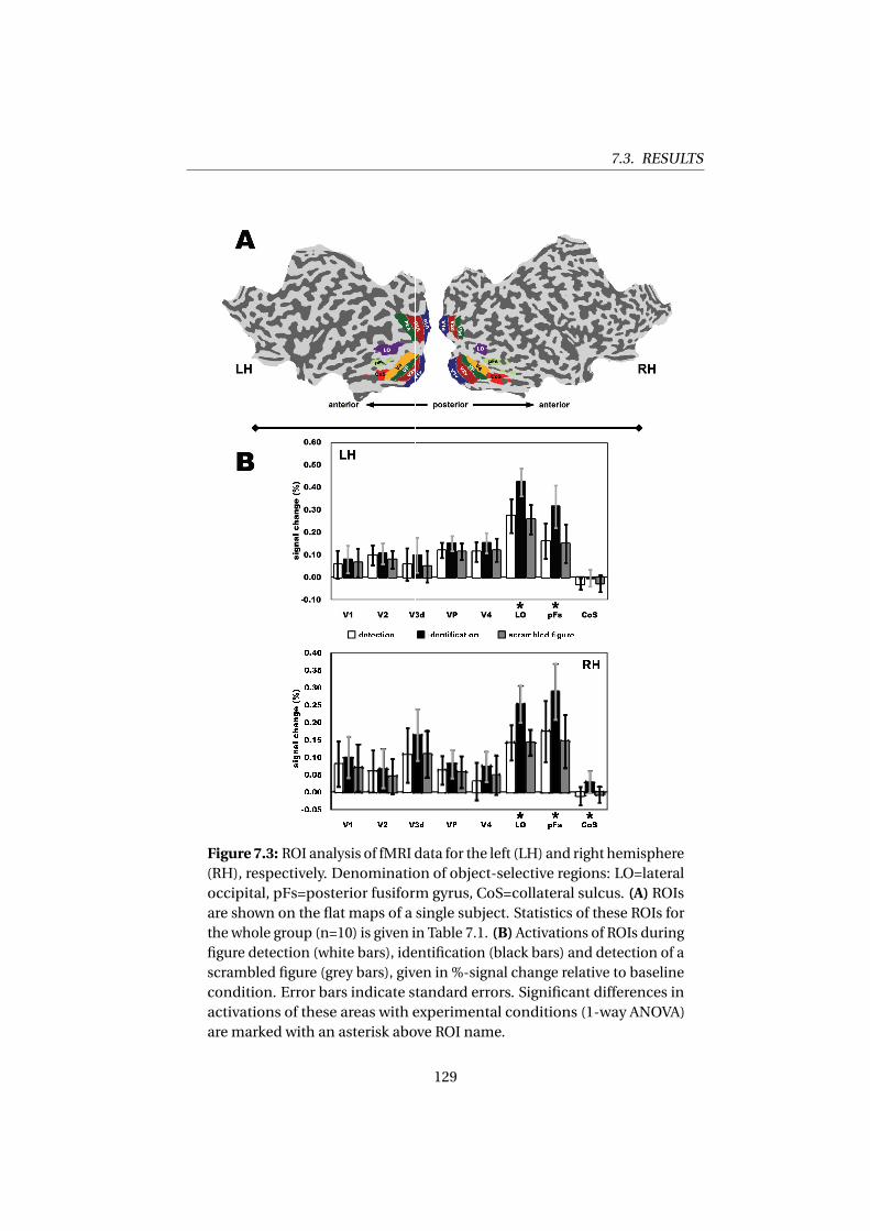
7.3. RESULTS
Figure 7.3: ROI analysis of fMRI data for the left (LH) and right hemisphere(RH), respectively. Denomination of object-selective regions: LO=lateraloccipital, pFs=posterior fusiform gyrus, CoS=collateral sulcus. (A) ROIsare shown on the flat maps of a single subject. Statistics of these ROIs forthe whole group (n=10) is given in Table 7.1. (B) Activations of ROIs duringfigure detection (white bars), identification (black bars) and detection of ascrambled figure (grey bars), given in %-signal change relative to baselinecondition. Error bars indicate standard errors. Significant differences inactivations of these areas with experimental conditions (1-way ANOVA)are marked with an asterisk above ROI name.
129
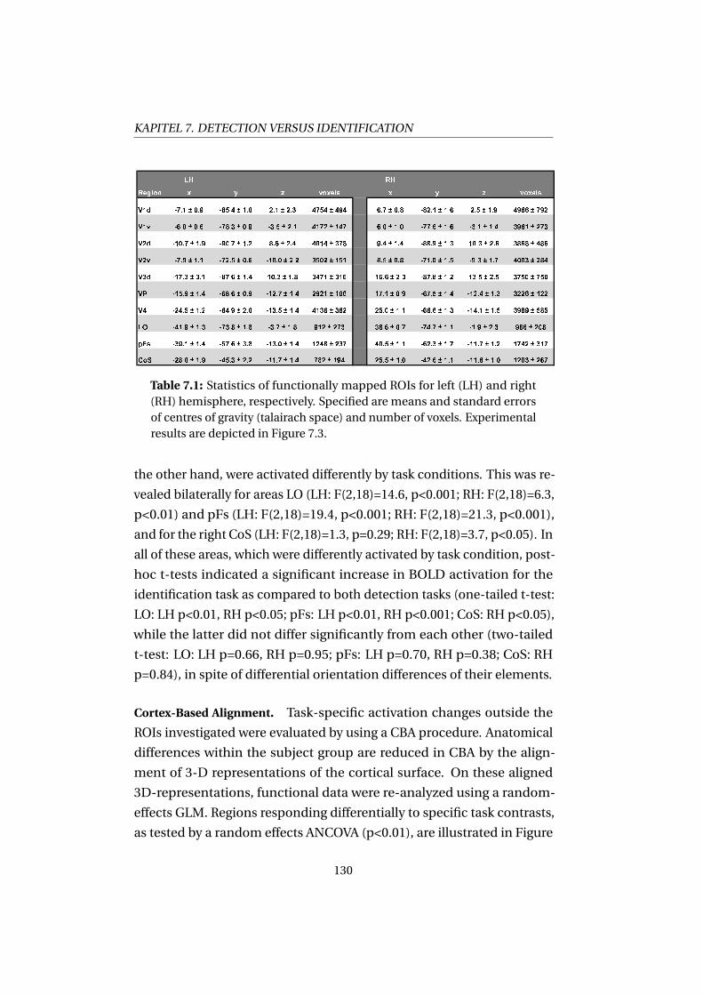
KAPITEL 7. DETECTION VERSUS IDENTIFICATION
Table 7.1: Statistics of functionally mapped ROIs for left (LH) and right(RH) hemisphere, respectively. Specified are means and standard errorsof centres of gravity (talairach space) and number of voxels. Experimentalresults are depicted in Figure 7.3.
the other hand, were activated differently by task conditions. This was re-
vealed bilaterally for areas LO (LH: F(2,18)=14.6, p<0.001; RH: F(2,18)=6.3,
p<0.01) and pFs (LH: F(2,18)=19.4, p<0.001; RH: F(2,18)=21.3, p<0.001),
and for the right CoS (LH: F(2,18)=1.3, p=0.29; RH: F(2,18)=3.7, p<0.05). In
all of these areas, which were differently activated by task condition, post-
hoc t-tests indicated a significant increase in BOLD activation for the
identification task as compared to both detection tasks (one-tailed t-test:
LO: LH p<0.01, RH p<0.05; pFs: LH p<0.01, RH p<0.001; CoS: RH p<0.05),
while the latter did not differ significantly from each other (two-tailed
t-test: LO: LH p=0.66, RH p=0.95; pFs: LH p=0.70, RH p=0.38; CoS: RH
p=0.84), in spite of differential orientation differences of their elements.
Cortex-Based Alignment. Task-specific activation changes outside the
ROIs investigated were evaluated by using a CBA procedure. Anatomical
differences within the subject group are reduced in CBA by the align-
ment of 3-D representations of the cortical surface. On these aligned
3D-representations, functional data were re-analyzed using a random-
effects GLM. Regions responding differentially to specific task contrasts,
as tested by a random effects ANCOVA (p<0.01), are illustrated in Figure
130
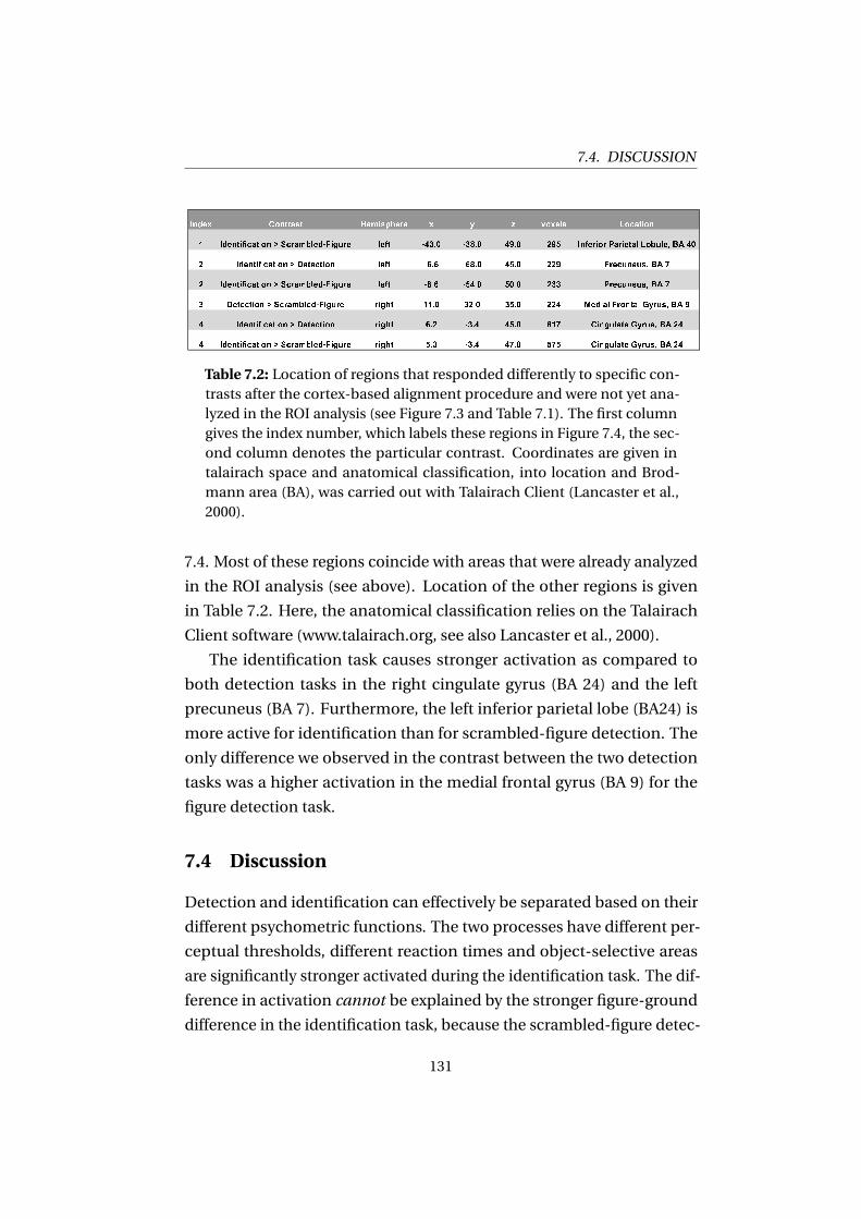
7.4. DISCUSSION
Table 7.2: Location of regions that responded differently to specific con-trasts after the cortex-based alignment procedure and were not yet ana-lyzed in the ROI analysis (see Figure 7.3 and Table 7.1). The first columngives the index number, which labels these regions in Figure 7.4, the sec-ond column denotes the particular contrast. Coordinates are given intalairach space and anatomical classification, into location and Brod-mann area (BA), was carried out with Talairach Client (Lancaster et al.,2000).
7.4. Most of these regions coincide with areas that were already analyzed
in the ROI analysis (see above). Location of the other regions is given
in Table 7.2. Here, the anatomical classification relies on the Talairach
Client software (www.talairach.org, see also Lancaster et al., 2000).
The identification task causes stronger activation as compared to
both detection tasks in the right cingulate gyrus (BA 24) and the left
precuneus (BA 7). Furthermore, the left inferior parietal lobe (BA24) is
more active for identification than for scrambled-figure detection. The
only difference we observed in the contrast between the two detection
tasks was a higher activation in the medial frontal gyrus (BA 9) for the
figure detection task.
7.4 Discussion
Detection and identification can effectively be separated based on their
different psychometric functions. The two processes have different per-
ceptual thresholds, different reaction times and object-selective areas
are significantly stronger activated during the identification task. The dif-
ference in activation cannot be explained by the stronger figure-ground
difference in the identification task, because the scrambled-figure detec-
131
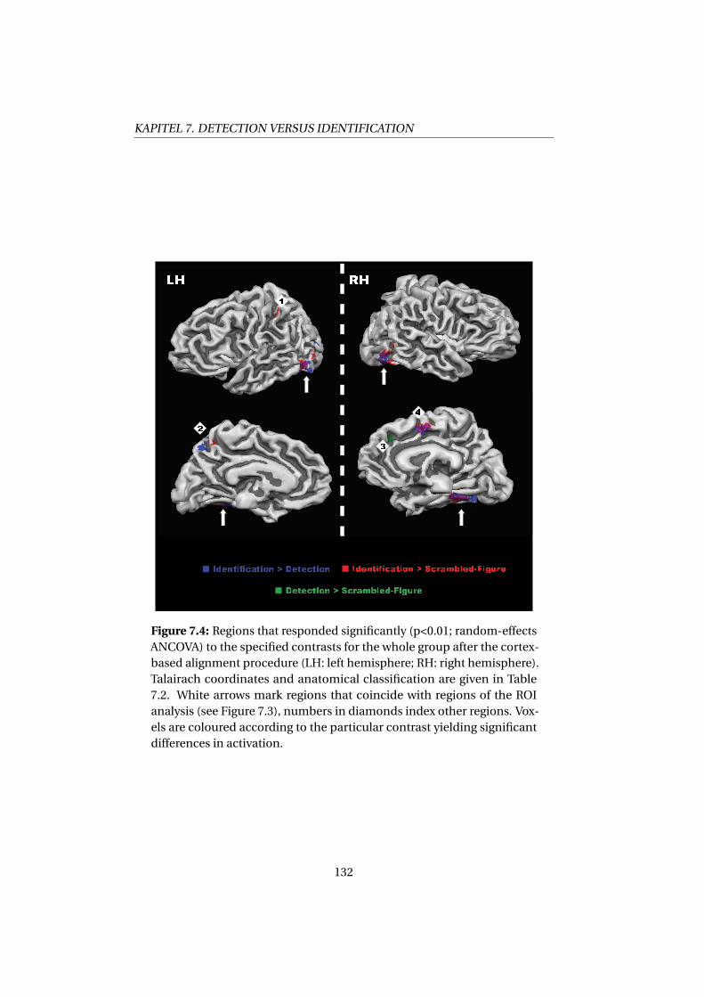
KAPITEL 7. DETECTION VERSUS IDENTIFICATION
Figure 7.4: Regions that responded significantly (p<0.01; random-effectsANCOVA) to the specified contrasts for the whole group after the cortex-based alignment procedure (LH: left hemisphere; RH: right hemisphere).Talairach coordinates and anatomical classification are given in Table7.2. White arrows mark regions that coincide with regions of the ROIanalysis (see Figure 7.3), numbers in diamonds index other regions. Vox-els are coloured according to the particular contrast yielding significantdifferences in activation.
132
7.4. DISCUSSION
tion condition has exactly the same figure-ground difference. Further
BOLD-effects corresponding to the different tasks appear in distinct pari-
etal, central and frontal regions of the cortex, as revealed by the cortex
based alignment. All these results challenge the conclusions drawn in
several previous studies, namely that detection and identification rely on
the samemechanism and that detecting an object is equivalent to identi-
fying it (Grill-Spector, 2003a,b; Grill-Spector et al., 2004; Grill-Spector &
Kanwisher, 2005). In the following, we will deal with this issue and further
interpret the results.
Differences inmapped visual areas. Location of functionally mapped ar-
eas (Table 7.1) is roughly in agreement with previous reports (for V1 to
V4 see Hasnain et al., 1998, ; for object-selective regions see Grill-Spector
et al., 2000). For analysis of activation (%-signal change) in these areas
each task was contrasted to the baseline condition. The bars in Figure
7.3B clearly show that neural processing is enhanced across all mapped
visual areas for all tasks. However, the low-level properties of the stimulus
are identical for the baseline condition and all other tasks, since the base-
line condition contained as many Gabor elements as the task conditions,
and also stimulus duration andmotor response were the same. Therefore,
only two factors can account for this enhanced activation: First, subjects
knew the current task (colour coded fixation point) and increased their
attentional allocation during the task conditions as compared to the base-
line condition. Indeed, it has been shown that attentionmodulates neural
activity on multiple levels of the visual system (for reviews see Kastner &
Pinsk, 2004; Rees & Lavie, 2001). Second, enhanced activations during the
task conditions might be caused by segregation processes which would
not occur in the baseline condition. Several studies reported the involve-
ment of the primary visual cortex (V1) in segregation processes (Kapadia
et al., 1995; Li et al., 2006; Murray et al., 2006; Polat et al., 1998; Zipser
et al., 1996) implying that figure-ground segregation maymodulate the
activity of neurons in V1 and subsequent areas. In the current study we
cannot dissociate between attentional and segregation effects, but since
attention here operates on the global level, because subjects did not know
133
KAPITEL 7. DETECTION VERSUS IDENTIFICATION
where the figure would appear, we conclude that the enhancement we
see has to be attributedmainly to attentional effects. Then, the amount
of attentional allocation should be roughly the same for detection and
identification, since all tasks were equally salient. Furthermore, it is ques-
tionable if the BOLD-signal, having a poor temporal resolution, reflects
the possible segregation effects mentioned above, since the presentation
time of the stimulus is rather short (80ms versus 2000ms fixation/answer
time) and the target saliency was limited (90%-correct responses).
Regions revealed by the cortex-based alignment. Consistent with the ROI-
analysis we found a higher hemodynamic response for the identification
task in voxel-clusters overlapping with object-selective areas LO, pFs
and CoS. Besides these, we observed further effects of specific contrasts
between the conditions in four distinct regions (illustrated in Figure 7.4).
All of these regions belong to a well known network that has been linked
with attentional control, working memory and conscious perception (for
a meta-analysis see Naghavi & Nyberg, 2005). All response differences we
observe were located unilaterally, which is common for this network.
In the left hemisphere, the identification task caused higher activa-
tions in parts of the precuneus (BA 7) and the inferior parietal lobe (BA
40). Activations in the vicinity of the coordinates we report here are of-
ten attributed to visuospatial processing (Deng et al., 2008), shifting of
attention (Booth et al., 2004; Corbetta et al., 1993; Le et al., 1998) and
spatial workingmemory (Buckner et al., 1996), but also their involvement
in non-spatial attentional allocation has been reported (for a review see
Kanwisher &Wojciulik, 2000). Attentional shifts to recognize the figures’
shape are only mandatory during the identification task, because here,
once the location of the target has been detected, spatial information has
to be integrated for successful recognition. In contrast, for detection the
target location is already sufficient to solve the task. Moreover, a region
comparable to the one we found in the inferior parietal lobe has been
related to orientation judgement (see area pCs in Altmann et al., 2005).
In our experiment this region showed enhanced activation during iden-
tification compared to detection of the scrambled figure, which can be
134
7.4. DISCUSSION
explained by the fact that orientation judgement aids the identification
process and the scrambled figure in turn had no orientation.
In the right hemisphere we found strongly overlapping regions of
enhanced activation for identification compared to both detection tasks
in the anterior cingulate gyrus (BA 24). Generally the anterior cingulate
cortex is considered to contribute to conflict monitoring and cognitive
control (Barch et al., 2001; Botvinick et al., 2001; Mayr, 2004). After per-
forming the experiments, subjects reported that during the identification
task they had to consciously suppress the reaction to push the answer key
according to the side where the figure appeared in order to answer cor-
rectly if it was symmetrical or asymmetrical. Indeed, a similar region has
been reported when subjects had to control opposite finger movement
(Paus et al., 1993).
The only difference we found between the two detection tasks was
an increased activation during figure detection in the right hemisphere
in the medial frontal gyrus (BA 9), close to the border to BA 6. A similar
frontal region (if not the same) was reported to be involved in orientation
judgements (Lee et al., 2005). This possible frontal involvement in ori-
entation judgement might be due to the fact that the figure and hence
its orientation is hardly visible in the figure detection task and therefore
higher cognitive control may be required to optimize performance. The
argument is similar to that for the observed parietal activation related to
orientation judgement: The scrambled figure has no orientation, but in
the figure detection condition it is useful to judge the figures’ orientation,
since its position always slightly crossed the vertical stimulus midline
and the orientation can be a hint to judge whether it is right or left.
Detection versus Identification: Same or different? The behavioural data
of this study corroborate that it is not necessary to recognize the shape
of an object to detect it. Indeed, the differences in the psychometric
functions reveal that even when subjects detect the figure correctly in 90
% of presentations, they are still only marginally above guessing proba-
bility regarding identification. This relation was robust across training
days. The differences in perceptual thresholds between the two tasks ob-
135
KAPITEL 7. DETECTION VERSUS IDENTIFICATION
viously are an intrinsic property of the visual system. Moreover, although
our tasks were saliency-matched, both detections were still significantly
faster (about 40 ms) than identification. These findings support the in-
terpretation of Mack et al. (2008) rather than that of Grill-Spector and
Kanwisher (2005). Our interpretation of partly separate neural mecha-
nisms is supported by additional behavioural studies showing that the
two processes differentially depend on the number of target elements
(Sagi & Julesz, 1984) and on cue combination (Meinhardt et al., 2006).
In addition to the behavioural evidence, we found different hemo-
dynamic responses in object-selective areas of the visual system. These
task-related differences cannot easily be attributed to propagation from
earlier visual areas, because we do not find task-related activation dif-
ferences in any of these. However, all areas showed increased activation
compared to the baseline condition, so we cannot definitely preclude
that object-selective areas are not involved in object detection. On the
other hand, we find this increased activation in all visual areas as com-
pared to the baseline condition and, as argued above, attentional and
segregation effects can account for this finding. A faint exception is the
region we termed CoS, which was activated only in the identification task
in the right hemisphere (compare Figure 7.3B). This special lateralized
activation (although small) strengthens the hypothesis that parts of the
brain are exclusively involved in recognition and not in detection. It will
be worthwhile in future studies investigating detection and identifica-
tion to especially scrutinize this region. Moreover, we did not observe a
hemodynamic response difference between the two detection tasks in
all visual areas considered indicating that the increased activation for
the identification task in object-selective areas reflects shape perception
and not figure-ground segregation. Shape perception was only relevant
(and possible) in the identification task. Therefore we conclude that the
activations of object-selective areas in both detection tasks rather reflect
the effort of the visual system to identify the target.
Further evidence for partly separate mechanisms for detection and
identification comes from fMRI studies investigating how the visual sys-
136
7.5. CONCLUSIONS
tem selects and encodes individual objects from a crowded scene. Here
the first process is termed object individuation and the latter object iden-
tification. In this framework, object individuation in a crowded scene is
the result of multiple, probably parallel detection. Consistent with the
results reported here, it has been found that both processes are realized
by two distinct mechanisms working together to enable fast and accurate
recognition performance (Xu & Chun, 2007; Xu, 2009).
7.5 Conclusions
The visual systemmay successfully detect an object even if identification
fails. We separated the two processes by measuring individual psycho-
metric functions and adjusting the figure-ground differences such that
subjects performed equally well in both tasks. Hence, stimulus salience
was matched for the two tasks. In our study, the BOLD-signal showed
larger activations for identification in object-selective subdivisions of the
LOC (LO and pFs) and an adjacent area (CoS). Area CoS was the only area
that seemed to be exclusively activated during identification. The ab-
sence of differences between the two detection tasks in object-selective
areas indicates that the additional activation during identification re-
flects shape recognition which was impossible during both detection
tasks. This finding underscores the fact that detection does not require
recognition and may rely on a partly separate mechanism. It will be
worthwhile to more specifically investigate if object selective areas are
in fact not essential for successful detection (e.g. by inducing virtual
lesions).
Acknowledgements
The authors like to thank M. Löbe and B. Dorgau for helping throughout
the data acquisition phase. We also like to thank D. Högl, C. Grimsen, P.
Erhard and D. Trenner for improving this study with valuable suggestions.
137

Literaturverzeichnis
Abele,M. & Fahle,M. (1995). Interactions between orientation, luminance
and color cues in figure-ground discrimination. Perception 24, 11.
Altmann, C. F., Grodd, W., Kourtzi, Z., Bulthoff, H. H. & Karnath, H. O.
(2005). Similar cortical correlates underlie visual object identification
and orientation judgment. Neuropsychologia 43(14), 2101–2108.
American Electroencephalographic Society (1994). Guideline thirteen:
guidelines for standard electrode position nomenclature. Journal of
Clinical Neurophysiology 11(1), 111–113.
Anllo-Vento, L. & Hillyard, S. A. (1996). Selective attention to the color
and direction of moving stimuli: electrophysiological correlates of hier-
archical feature selection. Perception & Psychophysics 58(2), 191–206.
Arthurs, O. J. & Boniface, S. (2002). Howwell do we understand the neural
origins of the fMRI bold signal? Trends in Neurosciences 25(1), 27–31.
Ashby, F. G. & Townsend, J. T. (1986). Varieties of perceptual independence.
Psychological Review 93(2), 154–179.
Assad, J. A. (2003). Neural coding of behavioral relevance in parietal
cortex. Current Opinion in Neurobiology 13(2), 194–197.
Bach, M. (1996). The freiburg visual acuity test–automatic measurement
of visual acuity. Optometry and Vision Science 73(1), 49–53.
Bach,M. &Meigen, T. (1992). Electrophysiological correlates of texture se-
gregation in the human visual evoked potential. Vision Research 32(3),
417–424.
139
LITERATURVERZEICHNIS
Bach, M. &Meigen, T. (1997). Similar electrophysiological correlates of
texture segregation induced by luminance, orientation, motion and
stereo. Vision Research 37(11), 1409–1414.
Bach, M. &Meigen, T. (1998). Electrophysiological correlates of human
texture segregation, an overview. Documenta Ophthalmologica. Ad-
vances in Ophthalmology 95(3-4), 335–347.
Bach,M., Schmitt, C., Quenzer, T.,Meigen, T. & Fahle,M. (2000). Summati-
on of texture segregation across orientation and spatial frequency: elec-
trophysiological and psychophysical findings. Vision Research 40(26),
3559–3566.
Barch, D. M., Braver, T. S., Akbudak, E., Conturo, T., Ollinger, J. & Snyder,
A. (2001). Anterior cingulate cortex and response conflict: effects of
response modality and processing domain. Cerebral Cortex 11(9), 837–
848.
Basar, E., Basar-Eroglu, C., Karakas, S. & Schurmann, M. (1999). Are
cognitive processes manifested in event-related gamma, alpha, theta
and delta oscillations in the EEG? Neuroscience Letters 259(3), 165–168.
Berger, H. (1929). Über das Elektroenkephalogramm des Menschen.
European Archives of Psychiatry and Clinical Neuroscience 87(1), 527–
570.
Bergmann, C. (1858). Anatomisches und Physiologisches über die Netz-
haut des Auges. In Henle, J. & Pfeufer, C. (Eds.). Zeitschrift für rationelle
Medicin (3 Ed.)., Band 2. Leipzig & Heidelberg: Winter’sche Verlags-
handlung, S. 83–108.
Birbaumer, N. & Schmidt, R. F. (2006). Biologische Psychologie : mit 41
Tabellen ; [Bonusmaterial imWeb]. Heidelberg: Springer Medizin.
Blake, A., Bulthoff, H. H. & Sheinberg, D. (1993). Shape from texture:
ideal observers and human psychophysics. Vision Research 33(12),
1723–1737.
140
LITERATURVERZEICHNIS
Booth, J. R., Burman, D. D., Meyer, J. R., Gitelman, D. R., Parrish, T. B.
& Mesulam, M. M. (2004). Development of brain mechanisms for
processing orthographic and phonologic representations. Journal of
Cognitive Neuroscience 16(7), 1234–1249.
Botvinick, M. M., Braver, T. S., Barch, D. M., Carter, C. S. & Cohen, J. D.
(2001). Conflict monitoring and cognitive control. Psychological Re-
view 108(3), 624–652.
Braddick, O. J., O’Brien, J. M., Wattam-Bell, J., Atkinson, J., Hartley, T.
& Turner, R. (2001). Brain areas sensitive to coherent visual motion.
Perception 30(1), 61–72.
Buckner, R. L., Raichle, M. E., Miezin, F. M. & Petersen, S. E. (1996). Func-
tional anatomic studies of memory retrieval for auditory words and
visual pictures. The Journal of Neuroscience 16(19), 6219–6235.
Bullier, J. (2001). Integratedmodel of visual processing. Brain Research
Reviews 36(2-3), 96–107.
Busch, N. A., Debener, S., Kranczioch, C., Engel, A. K. & Herrmann, C. S.
(2004). Size matters: effects of stimulus size, duration and eccentricity
on the visual gamma-band response. Clinical Neurophysiology 115(8),
1810–1820.
Busch, N. A., Herrmann, C. S., Muller, M. M., Lenz, D. & Gruber, T. (2006).
A cross-laboratory study of event-related gamma activity in a standard
object recognition paradigm. NeuroImage 33(4), 1169–1177.
Busch, N. A., Schadow, J., Frund, I. & Herrmann, C. S. (2006). Time-
frequency analysis of target detection reveals an early interface bet-
ween bottom-up and top-down processes in the gamma-band. Neu-
roImage 29(4), 1106–1116.
Caputo, G. & Casco, C. (1999). A visual evoked potential correlate of global
figure-ground segmentation. Vision Research 39(9), 1597–1610.
141
LITERATURVERZEICHNIS
Carey, D. P., Dijkerman, H. C., Murphy, K. J., Goodale, M. A. & Milner,
A. D. (2006). Pointing to places and spaces in a patient with visual form
agnosia. Neuropsychologia 44(9), 1584–1594.
Corbetta, M., Miezin, F. M., Dobmeyer, S., Shulman, G. L. & Petersen, S. E.
(1990). Attentional modulation of neural processing of shape, color,
and velocity in humans. Science 248(4962), 1556–1559.
Corbetta, M., Miezin, F. M., Shulman, G. L. & Petersen, S. E. (1993). A
PET study of visuospatial attention. The Journal of Neuroscience 13(3),
1202–1226.
Dale, A. M., Fischl, B. & Sereno, M. I. (1999). Cortical surface-based
analysis. i. segmentation and surface reconstruction. NeuroImage 9(2),
179–194.
Deco, G. & Rolls, E. T. (2004). A neurodynamical cortical model of visual
attention and invariant object recognition. Vision Research 44(6), 621–
642.
Deng, Y., Booth, J. R., Chou, T. L., Ding, G. S. & Peng, D. L. (2008). Item-
specific and generalization effects on brain activation when learning
chinese characters. Neuropsychologia 46(7), 1864–1876.
Doniger, G. M., Foxe, J. J., Murray, M. M., Higgins, B. A., Snodgrass, J. G.,
Schroeder, C. E. & Javitt, D. C. (2000). Activation timecourse of ventral vi-
sual streamobject-recognition areas: high density electricalmapping of
perceptual closure processes. Journal of Cognitive Neuroscience 12(4),
615–621.
Doniger, G. M., Foxe, J. J., Schroeder, C. E., Murray, M. M., Higgins, B. A. &
Javitt, D. C. (2001). Visual perceptual learning in human object reco-
gnition areas: a repetition priming study using high-density electrical
mapping. NeuroImage 13(2), 305–313.
Eckhorn, R., Bauer, R., Jordan, W., Brosch, M., Kruse, W., Munk, M. &
Reitboeck, H. J. (1988). Coherent oscillations: a mechanism of feature
142
LITERATURVERZEICHNIS
linking in the visual cortex? Multiple electrode and correlation analyses
in the cat. Biological Cybernetics 60(2), 121–130.
Edelman, G. M. & Griese, F. (1993). Unser Gehirn - ein dynamisches
System : die Theorie des neuronalen Darwinismus und die biologischen
Grundlagen der Wahrnehmung. München: Piper.
Ehrenstein, W. H. & Ehrenstein, A. (1999). Psychophysical Methods. In
Windhorst, U. & Johansson, H. (Eds.). Modern techniques in neuros-
cience research. Berlin: Springer, S. 1211–1241.
Fabiani, M., Gratton, G. & Coles, M. G. H. (2000). Event-related brain po-
tentials: Methods, theory, and applications. In Cacioppo, J. T., Tassinary,
L. G. & Berntson, G. G. (Eds.). Handbook of psychophysiology (2 Ed.).
Cambridge: Cambridge University Press, S. 53–84.
Fahle, M., Quenzer, T., Braun, C. & Spang, K. (2003). Feature-specific elec-
trophysiological correlates of texture segregation. Vision Research 43(1),
7–19.
Fechner, G. T. (1860). Elemente der Psychophysik. Leipzig: Breitkopf und
Härtel.
Ffytche, D. H. & Zeki, S. (1996). Brain activity related to the perception of
illusory contours. NeuroImage 3(2), 104–108.
Fischl, B., Sereno, M. I. & Dale, A. M. (1999). Cortical surface-based
analysis. ii: Inflation, flattening, and a surface-based coordinate system.
NeuroImage 9(2), 195–207.
Georgieva, S., Peeters, R., Kolster, H., Todd, J. T. & Orban, G. A. (2009). The
processing of three-dimensional shape from disparity in the human
brain. The Journal of Neuroscience 29(3), 727–742.
Goebel, R., Esposito, F. & Formisano, E. (2006). Analysis of functional
image analysis contest (FIAC) data with Brainvoyager QX: From single-
subject to cortically aligned group general linear model analysis and
self-organizing group independent component analysis. Human Brain
Mapping 27(5), 392–401.
143
LITERATURVERZEICHNIS
Green, D. M. & Swets, J. A. (1988). Signal detection theory and psychophy-
sics. Los Altos, CA: Peninsula Publ.
Grill-Spector, K. (2003a). The functional organization of the ventral visual
pathway and its relationship to object recognition. In Kanwisher, N. &
Duncan, J. (Eds.). Functional neuroimaging of visual cognition: attenti-
on and performance XX. Oxford: Oxford University Press, S. 169–193.
Grill-Spector, K. (2003b). The neural basis of object perception. Current
Opinion in Neurobiology 13(2), 159–166.
Grill-Spector, K. & Kanwisher, N. (2005). Visual recognition: as soon as
you know it is there, you know what it is. Psychological Science 16(2),
152–160.
Grill-Spector, K., Knouf, N. & Kanwisher, N. (2004). The fusiform face area
subserves face perception, not generic within-category identification.
Nature Neuroscience 7(5), 555–562.
Grill-Spector, K., Kushnir, T., Hendler, T. &Malach, R. (2000). The dyna-
mics of object-selective activation correlate with recognition perfor-
mance in humans. Nature Neuroscience 3(8), 837–843.
Hasnain, M. K., Fox, P. T. & Woldorff, M. G. (1998). Intersubject varia-
bility of functional areas in the human visual cortex. Human Brain
Mapping 6(4), 301–315.
Heeger, D. J. & Ress, D. (2004). Neuronal correlates of visual attention and
perception. In Gazzaniga, M. S., Ivry, R. B., Mangun, G. R. & Steven,
M. S. (Eds.). Cognitive neuroscience: the biology of the mind (3 Ed.).
New York, NY: Norton, S. 339–350.
Heinrich, S. P., Andres, M. & Bach, M. (2007). Attention and visual texture
segregation. Journal of Vision 7(6), 6.
Herrmann, C. S. & Bosch, V. (2001). Gestalt perceptionmodulates early
visual processing. Neuroreport 12(5), 901–904.
144
LITERATURVERZEICHNIS
Herrmann, C. S., Grigutsch, M. & Busch, N. A. (2005). EEG oscillations
and wavelet analysis. In Handy, T. (Ed.). Event-Related Potentials: A
Methods Handbook. Cambridge, Mass: MIT Press, S. 229–259.
Hillis, J. M., Watt, S. J., Landy, M. S. & Banks, M. S. (2004). Slant from
texture and disparity cues: optimal cue combination. Journal of Visi-
on 4(12), 967–992.
Hopfinger, J. B., Khoe, W. & Song, A. (2005). Combining Electrophysiology
with Structural and Functional Neuroimaging: ERPs, PET, MRI, and fM-
RI. In Handy, T. (Ed.). Event-Related Potentials: A Methods Handbook.
Cambridge, Mass: MIT Press, S. 345–379.
Hubel, D. H. & Livingstone, M. S. (1987). Segregation of form, color,
and stereopsis in primate area 18. The Journal of Neuroscience 7(11),
3378–3415.
Huettel, S. A., Song, A. W. & McCarthy, G. (2004). Functional magnetic
resonance imaging. Sunderland, Mass.: Sinauer.
Itti, L. & Koch, C. (2001). Computational modelling of visual attention.
Nature Reviews Neuroscience 2(3), 194–203.
Jacobs, R. A. & Fine, I. (1999). Experience-dependent integration of tex-
ture andmotion cues to depth. Vision Research 39(24), 4062–4075.
Kaas, J. H. (1996). Theories of visual cortex organization in primates:
areas of the third level. Progress in Brain Research 112, 213–221.
Kaas, J. H. & Lyon, D. C. (2001). Visual cortex organization in primates:
theories of V3 and adjoining visual areas. Progress in Brain Research 134,
285–295.
Kahana, M. J., Seelig, D. & Madsen, J. R. (2001). Theta returns. Current
Opinion in Neurobiology 11(6), 739–744.
Kandel, E. R., Schwartz, J. H. & Jessell, T. M. (2000). Principles of neural
science. New York: McGraw-Hill, Health Professions Division.
145
LITERATURVERZEICHNIS
Kanwisher, N. &Wojciulik, E. (2000). Visual attention: insights from brain
imaging. Nature Reviews Neuroscience 1(2), 91–100.
Kapadia, M. K., Ito, M., Gilbert, C. D. &Westheimer, G. (1995). Improve-
ment in visual sensitivity by changes in local context: parallel studies in
human observers and in V1 of alert monkeys. Neuron 15(4), 843–856.
Kastner, S. & Pinsk, M. A. (2004). Visual attention as a multilevel selection
process. Cognitive, Affective & Behavioral Neuroscience 4(4), 483–500.
Kastner, S., Schneider, K. A. & Wunderlich, K. (2006). Beyond a relay
nucleus: neuroimaging views on the human LGN. Progress in Brain
Research 155, 125–143.
Key, A. P., Dove, G. O. &Maguire, M. J. (2005). Linking brainwaves to the
brain: an ERP primer. Developmental Neuropsychology 27(2), 183–215.
Kolb, H. (2003). How the retina works. American Scientist 91(1), 28–35.
Kotsoni, E., Csibra, G., Mareschal, D. & Johnson, M. H. (2007). Electro-
physiological correlates of common-onset visual masking. Neuropsy-
chologia 45(10), 2285–2293.
Kubovy, M. & Cohen, D. J. (2001). What boundaries tell us about binding.
Trends in Cognitive Sciences 5(3), 93–95.
Kubovy, M., Cohen, D. J. & Hollier, J. (1999). Feature integration that
routinely occurs without focal attention. Psychonomic Bulletin & Re-
view 6(2), 183–203.
Lamme, V. A. & Roelfsema, P. R. (2000). The distinct modes of vision
offered by feedforward and recurrent processing. Trends in Neuros-
ciences 23(11), 571–579.
Lamme, V. A., Super, H. & Spekreijse, H. (1998). Feedforward, horizon-
tal, and feedback processing in the visual cortex. Current Opinion in
Neurobiology 8(4), 529–535.
146
LITERATURVERZEICHNIS
Lamme, V. A., Van Dijk, B. W. & Spekreijse, H. (1992). Texture segregation
is processed by primary visual cortex in man and monkey. evidence
from VEP experiments. Vision Research 32(5), 797–807.
Lancaster, J. L., Woldorff, M. G., Parsons, L. M., Liotti, M., Freitas, C. S.,
Rainey, L., Kochunov, P. V., Nickerson, D.,Mikiten, S. A. & Fox, P. T. (2000).
Automated talairach atlas labels for functional brain mapping. Human
Brain Mapping 10(3), 120–131.
Landy, M. S. & Kojima, H. (2001). Ideal cue combination for localizing
texture-defined edges. Journal of the Optical Society of America A 18(9),
2307–2320.
Lauterbur, P. C. (1973). Image formation by induced local interactions:
Examples employing nuclear magnetic resonance. Nature 242(5394),
190–191.
Le, T. H., Pardo, J. V. & Hu, X. (1998). 4 t-fMRI study of nonspatial shifting
of selective attention: cerebellar and parietal contributions. Journal of
Neurophysiology 79(3), 1535–1548.
Lee, T. M., Liu, H. L., Hung, K. N., Pu, J., Ng, Y. B., Mak, A. K., Gao, J. H.
& Chan, C. C. (2005). The cerebellum’s involvement in the judgment
of spatial orientation: a functional magnetic resonance imaging study.
Neuropsychologia 43(13), 1870–1877.
Lee, T. S. & Nguyen, M. (2001). Dynamics of subjective contour formation
in the early visual cortex. Proceedings of the National Academy of
Sciences of the United States of America 98(4), 1907–1911.
Lennie, P. (1980). Parallel visual pathways: a review. Vision Research 20(7),
561–594.
Leonards, U. & Singer, W. (2000). Conjunctions of colour, luminance and
orientation: the role of colour and luminance contrast on saliency and
proximity grouping in texture segregation. Spatial Vision 13(1), 87–105.
Li, W., Piech, V. & Gilbert, C. D. (2006). Contour saliency in primary visual
cortex. Neuron 50(6), 951–962.
147
LITERATURVERZEICHNIS
Livingstone, M. &Hubel, D. (1988). Segregation of form, color, movement,
and depth: anatomy, physiology, and perception. Science 240(4853),
740–749.
Logothetis, N. K. (2002). The neural basis of the blood-oxygen-level-
dependent functional magnetic resonance imaging signal. Philoso-
phical Transactions of the Royal Society of London. Series B 357(1424),
1003–1037.
Luck, S. J. (2005). An introduction to the event-related potential technique.
Cambridge, Mass: MIT Press.
Mack, M. L., Gauthier, I., Sadr, J. & Palmeri, T. J. (2008). Object detection
and basic-level categorization: sometimes you know it is there before
you know what it is. Psychonomic Bulletin & Review 15(1), 28–35.
Macmillan, N. A. & Creelman, C. D. (1991). Detection theory : a user’s
guide. Cambridge: Cambridge Univ. Press.
Macmillan, N. A. & Creelman, C. D. (2005). Detection theory : a user’s
guide. Mahwah, NJ: Lawrence Erlbaum Associates.
Malach, R., Reppas, J. B., Benson, R. R., Kwong, K. K., Jiang, H., Kennedy,
W. A., Ledden, P. J., Brady, T. J., Rosen, B. R. & Tootell, R. B. (1995). Object-
related activity revealed by functional magnetic resonance imaging
in human occipital cortex. Proceedings of the National Academy of
Sciences of the United States of America 92(18), 8135–8139.
Mansfield, P. &Maudsley, A. A. (1976). Line scan proton spin imaging in
biological structures by NMR. Physics in Medicine and Biology 21(5),
847–852.
Mathes, B. & Fahle, M. (2007). The electrophysiological correlate of con-
tour integration is similar for color and luminance mechanisms. Psy-
chophysiology 44(2), 305–322.
Mathes, B., Trenner, D. & Fahle, M. (2006). The electrophysiological
correlate of contour integration is modulated by task demands. Brain
Research 1114(1), 98–112.
148
LITERATURVERZEICHNIS
Maunsell, J. H. & Treue, S. (2006). Feature-based attention in visual cortex.
Trends in Neurosciences 29(6), 317–322.
Mayr, U. (2004). Conflict, consciousness, and control. Trends in Cognitive
Sciences 8(4), 145–148.
McCarthy, G. & Donchin, E. (1981). A metric for thought: a comparison
of p300 latency and reaction time. Science 211(4477), 77–80.
McKeefry, D. J. & Zeki, S. (1997). The position and topography of the
human colour centre as revealed by functional magnetic resonance
imaging. Brain: A Journal of Neurology 120, 2229–2242.
Mecklinger, A. & Muller, N. (1996). Dissociations in the processing of
”what” and ”where” information in working memory: An event-related
potential analysis. Journal of Cognitive Neuroscience 8(5), 453–473.
Meinhardt, G. & Persike, M. (2003). Strength of feature contrast mediates
interaction among feature domains. Spatial Vision 16(5), 459–478.
Meinhardt, G., Persike, M., Mesenholl, B. & Hagemann, C. (2006). Cue
combination in a combined feature contrast detection and figure iden-
tification task. Vision Research 46(23), 3977–3993.
Meinhardt, G., Schmidt,M., Persike,M. &Roers, B. (2004). Feature synergy
depends on feature contrast and objecthood. Vision Research 44(16),
1843–1850.
Merigan, W. H. & Maunsell, J. H. (1993). How parallel are the primate
visual pathways? Annual Review of Neuroscience 16, 369–402.
Mima, T., Oluwatimilehin, T., Hiraoka, T. &Hallett, M. (2001). Transient in-
terhemispheric neuronal synchrony correlates with object recognition.
The Journal of Neuroscience 21(11), 3942–3948.
Mishkin, M., Ungerleider, L. & Macko, K. (1983). Object vision and spatial
vision: two cortical pathways. Trends in Neurosciences 6, 414–417.
149
LITERATURVERZEICHNIS
Moutoussis, K. & Zeki, S. (2008). Motion processing, directional selectivity,
and conscious visual perception in the human brain. Proceedings of the
National Academy of Sciences of the United States of America 105(42),
16362–16367.
Murray, M.M., Foxe, D.M., Javitt, D. C. & Foxe, J. J. (2004). Setting bounda-
ries: brain dynamics of modal and amodal illusory shape completion
in humans. The Journal of Neuroscience 24(31), 6898–6903.
Murray, M. M., Imber, M. L., Javitt, D. C. & Foxe, J. J. (2006). Boundary
completion is automatic and dissociable from shape discrimination.
The Journal of Neuroscience 26(46), 12043–12054.
Murray, M. M., Wylie, G. R., Higgins, B. A., Javitt, D. C., Schroeder, C. E.
& Foxe, J. J. (2002). The spatiotemporal dynamics of illusory contour
processing: combined high-density electrical mapping, source analysis,
and functional magnetic resonance imaging. The Journal of Neuros-
cience 22(12), 5055–5073.
Murray, S. O., Boyaci, H. & Kersten, D. (2006). The representation of
perceived angular size in human primary visual cortex. Nature Neuros-
cience 9(3), 429–434.
Naghavi, H. R. & Nyberg, L. (2005). Common fronto-parietal activity in at-
tention, memory, and consciousness: shared demands on integration?
Consciousness and Cognition 14(2), 390–425.
Nothdurft, H. (2000). Salience from feature contrast: additivity across
dimensions. Vision Research 40(10-12), 1183–1201.
O’Craven, K. M., Downing, P. E. & Kanwisher, N. (1999). fMRI evidence for
objects as the units of attentional selection. Nature 401(6753), 584–587.
Ohman, A., Flykt, A. & Esteves, F. (2001). Emotion drives attention: de-
tecting the snake in the grass. Journal of Experimental Psychology:
General 130(3), 466–478.
150
LITERATURVERZEICHNIS
Ohman, A. & Mineka, S. (2001). Fears, phobias, and preparedness: to-
ward an evolved module of fear and fear learning. Psychological Re-
view 108(3), 483–522.
Oruc, I., Maloney, L. T. & Landy, M. S. (2003). Weighted linear cue com-
bination with possibly correlated error. Vision Research 43(23), 2451–
2468.
Palmer, S. E. (2002). Vision science : photons to phenomenology. Cam-
bridge, Mass: MIT Press.
Pashler, H. (1988). Cross-dimensional interaction and texture segregation.
Perception & Psychophysics 43(4), 307–318.
Pashler, H. E. (1999). The psychology of attention. Cambridge, Mass.: MIT
Press.
Pasupathy, A. & Connor, C. E. (2002). Population coding of shape in area
V4. Nature Neuroscience 5(12), 1332–1338.
Paus, T., Petrides, M., Evans, A. C. &Meyer, E. (1993). Role of the human
anterior cingulate cortex in the control of oculomotor, manual, and
speech responses: a positron emission tomography study. Journal of
Neurophysiology 70(2), 453–469.
Perkins, D. N. (1983). Why the Human Perceiver Is a BadMachine. In Beck,
J., Hope, B. & Rosenfeld, A. (Eds.). Human andmachine vision, Notes
and reports in computer science and applied mathematics, Band 8.
Orlando, Fla: Academic Press, S. 341–364.
Persike, M. &Meinhardt, G. (2006). Synergy of features enables detection
of texture defined figures. Spatial Vision 19(1), 77–102.
Peterson, M. & Gibson, B. (1994). Must figure-ground organization
precede object recognition? An assumption in peril. Psychological
Science 5(5), 253–259.
Phillips, W. A. (2001). Contextual modulation and dynamic grouping in
perception. Trends in Cognitive Sciences 5(3), 95–97.
151
LITERATURVERZEICHNIS
Phillips, W. A. & Craven, B. J. (2000). Interactions between coincident
and orthogonal cues to texture boundaries. Perception & Psychophy-
sics 62(5), 1019–1038.
Picton, T. W. (1992). The P300 wave of the human event-related potential.
Journal of Clinical Neurophysiology 9(4), 456–479.
Polat, U., Mizobe, K., Pettet, M. W., Kasamatsu, T. & Norcia, A. M. (1998).
Collinear stimuli regulate visual responses depending on cell’s contrast
threshold. Nature 391(6667), 580–584.
Polich, J. (2004). Clinical application of the P300 event-related brain
potential. Physical Medicine and Rehabilitation Clinics of North Ameri-
ca 15(1), 133–161.
Polich, J. & Kok, A. (1995). Cognitive and biological determinants of P300:
an integrative review. Biological Psychology 41(2), 103–146.
Rees, G. & Lavie, N. (2001). What can functional imaging reveal about
the role of attention in visual awareness? Neuropsychologia 39(12),
1343–1353.
Reynolds, J. H. & Chelazzi, L. (2004). Attentional modulation of visual
processing. Annual Review of Neuroscience 27, 611–647.
Rivest, J. & Cavanagh, P. (1996). Localizing contours defined bymore than
one attribute. Vision Research 36(1), 53–66.
Roelfsema, P. R., Lamme, V. A., Spekreijse, H. & Bosch, H. (2002). Figure-
ground segregation in a recurrent network architecture. Journal of
Cognitive Neuroscience 14(4), 525–537.
Sagi, D. & Julesz, B. (1984). Detection versus discrimination of visual
orientation. Perception 13(5), 619–628.
Samar, V. J., Bopardikar, A., Rao, R. & Swartz, K. (1999). Wavelet analysis
of neuroelectric waveforms: a conceptual tutorial. Brain and Langua-
ge 66(1), 7–60.
152
LITERATURVERZEICHNIS
Sarnthein, J., Petsche, H., Rappelsberger, P., Shaw, G. L. & von Stein, A.
(1998). Synchronization between prefrontal and posterior association
cortex during human working memory. Proceedings of the National
Academy of Sciences of the United States of America 95(12), 7092–7096.
Schenk, T. (2006). An allocentric rather than perceptual deficit in patient
DF. Nature Neuroscience 9(11), 1369–1370.
Scholl, B. J. (2001). Objects and attention: the state of the art. Cogniti-
on 80(1-2), 1–46.
Sehatpour, P., Molholm, S., Javitt, D. C. & Foxe, J. J. (2006). Spatiotempo-
ral dynamics of human object recognition processing: an integrated
high-density electrical mapping and functional imaging study of "clos-
ure"processes. NeuroImage 29(2), 605–618.
Senkowski, D. & Herrmann, C. S. (2002). Effects of task difficulty on evo-
ked gamma activity and ERPs in a visual discrimination task. Clinical
Neurophysiology 113(11), 1742–1753.
Sherman, S. M. (2007). The thalamus is more than just a relay. Current
Opinion in Neurobiology 17(4), 417–422.
Shipp, S. & Zeki, S. (2002a). The functional organization of area V2, I:
specialization across stripes and layers. Visual Neuroscience 19(2),
187–210.
Shipp, S. & Zeki, S. (2002b). The functional organization of area V2, II:
the impact of stripes on visual topography. Visual Neuroscience 19(2),
211–231.
Shoji, H. & Ozaki, H. (2006). Topographic change in ERP due to discrimi-
nation of geometric figures in the peripheral visual field. International
Journal of Psychophysiology 62(1), 115–121.
Sincich, L. C. & Horton, J. C. (2002). Divided by cytochrome oxidase: a
map of the projections from V1 to V2 in macaques. Science 295(5560),
1734–1737.
153
LITERATURVERZEICHNIS
Singer, W. (1999). Neurobiology: Striving for coherence. Nature 397(6718),
391, 393.
Slotnick, S. D. (2005). Source Localization of ERP Generators. In Handy,
T. (Ed.). Event-Related Potentials: AMethods Handbook. Cambridge,
Mass: MIT Press, S. 149–166.
Spang, K. &Morgan, M. (2008). Cortical correlates of stereoscopic depth
produced by temporal delay. Journal of Vision 8(9), 10.1–12.
Suder, K. & Worgotter, F. (2000). The control of low-level information flow
in the visual system. Reviews in the Neurosciences 11(2-3), 127–146.
Talairach, J., Tournoux, P., Missir, O. & Turak, B. (1993). Referentially
oriented cerebral MRI anatomy: an atlas of stereotaxic anatomical cor-
relations for gray and white matter. Stuttgart: Thieme u.a.
Tallon-Baudry, C. & Bertrand, O. (1999). Oscillatory gamma activity in
humans and its role in object representation. Trends in Cognitive
Sciences 3(4), 151–162.
Tallon-Baudry, C., Bertrand, O., Peronnet, F. & Pernier, J. (1998). Induced
gamma-band activity during the delay of a visual short-termmemory
task in humans. The Journal of Neuroscience 18(11), 4244–4254.
Tanner, W. P. (1956). Theory of recognition. Journal of the Acoustical
Society of America 28, 882–888.
Thorpe, S., Fize, D. &Marlot, C. (1996). Speed of processing in the human
visual system. Nature 381(6582), 520–522.
Thorpe, S. J. & Fabre-Thorpe, M. (2001). Neuroscience. seeking categories
in the brain. Science 291(5502), 260–263.
Tootell, R. B., Mendola, J. D., Hadjikhani, N. K., Ledden, P. J., Liu, A. K.,
Reppas, J. B., Sereno, M. I. & Dale, A. M. (1997). Functional analysis of
V3A and related areas in human visual cortex. The Journal of Neuros-
cience 17(18), 7060–7078.
154
LITERATURVERZEICHNIS
Tootell, R. B., Mendola, J. D., Hadjikhani, N. K., Liu, A. K. & Dale, A. M.
(1998). The representation of the ipsilateral visual field in human
cerebral cortex. Proceedings of the National Academy of Sciences of the
United States of America 95(3), 818–824.
Tootell, R. B., Silverman, M. S., Switkes, E. & Valois, R. L. D. (1982). Deoxy-
glucose analysis of retinotopic organization in primate striate cortex.
Science 218(4575), 902–904.
Torrence, C. & Compo, G. P. (1998). A practical guide to wavelet analysis.
Bulletin of the American Meteorological Society 79, 61–78.
Treisman, A. M. & Gelade, G. (1980). A feature-integration theory of
attention. Cognitive Psychology 12(1), 97–136.
Treue, S. (2003). Visual attention: the where, what, how and why of
saliency. Current Opinion in Neurobiology 13(4), 428–432.
Treutwein, B. (1995). Adaptive psychophysical procedures. Vision Rese-
arch 35(17), 2503–2522.
Triesch, J., Ballard, D. H. & Jacobs, R. A. (2002). Fast temporal dynamics
of visual cue integration. Perception 31(4), 421–434.
Tsujimoto, S. & Tayama, T. (2004). Independent mechanisms for dividing
attention between the motion and the color of dynamic random dot
patterns. Psychological Research 68(4), 237–244.
Van Essen, D. C., Anderson, C. H. & Felleman, D. J. (1992). Information
processing in the primate visual system: an integrated systems perspec-
tive. Science 255(5043), 419–423.
van Mierlo, C. M., Brenner, E. & Smeets, J. B. (2007). Temporal aspects of
cue combination. Journal of Vision 7(7), 8.1–11.
von Stein, A. & Sarnthein, J. (2000). Different frequencies for different sca-
les of cortical integration: from local gamma to long range alpha/theta
synchronization. International Journal of Psychophysiology 38(3), 301–
313.
155
LITERATURVERZEICHNIS
Warnking, J., Dojat, M., Guerin-Dugue, A., Delon-Martin, C., Olympieff,
S., Richard, N., Chehikian, A. & Segebarth, C. (2002). fMRI retinotopic
mapping–step by step. NeuroImage 17(4), 1665–1683.
Watson, A. B. & Fitzhugh, A. (1990). The method of constant stimuli is
inefficient. Perception & Psychophysics 47(1), 87–91.
Watson, A. B. & Pelli, D. G. (1983). QUEST: a bayesian adaptive psycho-
metric method. Perception & Psychophysics 33(2), 113–120.
Wolfe, J. M. (2000). Visual attention. In DeValois, K. K. (Ed.). Seeing. San
Diego: Acad. Press, S. 335–386.
Xu, Y. (2009). Distinctive neural mechanisms supporting visual object in-
dividuation and identification. Journal of Cognitive Neuroscience 21(3),
511–518.
Xu, Y. & Chun, M. M. (2007). Visual grouping in human parietal cortex.
Proceedings of the National Academy of Sciences of the United States of
America 104(47), 18766–18771.
Yantis, S. & Serences, J. T. (2003). Cortical mechanisms of space-based
and object-based attentional control. Current Opinion in Neurobiolo-
gy 13(2), 187–193.
Zeki, S. (1980). The representation of colours in the cerebral cortex.
Nature 284(5755), 412–418.
Zeki, S., Watson, J. D., Lueck, C. J., Friston, K. J., Kennard, C. & Frackowiak,
R. S. (1991). A direct demonstration of functional specialization in
human visual cortex. The Journal of Neuroscience 11(3), 641–649.
Zeki, S. M. (1973). Colour coding in rhesus monkey prestriate cortex.
Brain Research 53(2), 422–427.
Zeki, S. M. (1974). Functional organization of a visual area in the posterior
bank of the superior temporal sulcus of the rhesusmonkey. The Journal
of Physiology 236(3), 549–573.
156
LITERATURVERZEICHNIS
Zeki, S. M. (1978). Functional specialisation in the visual cortex of the
rhesus monkey. Nature 274(5670), 423–428.
Zipser, K., Lamme, V. A. & Schiller, P. H. (1996). Contextual modulation in
primary visual cortex. The Journal of Neuroscience 16(22), 7376–7389.
Zwickel, T., Wachtler, T. & Eckhorn, R. (2007). Coding the presence of
visual objects in a recurrent neural network of visual cortex. Bio Sys-
tems 89(1-3), 216–226.
157


Anhang
159

ABKÜRZUNGEN
Abkürzungen
Physikalische Einheiten
cpd Schwingungen pro Sehwinkelgrad (aus dem engl. cycles
per degree)
dB Dezibel
g Gramm
Hz Hertz
ms Millisekunde
oct Oktave (aus dem engl. octave)
s Sekunde
T Tesla
V Volt (mV=Millivolt; μV=Microvolt)
Andere Abkürzungen
ALM/GLM allgemeines lineares Modell (engl. general linear model)
ANOVA Varianzanalyse (aus dem engl. analysis of variance)
BOLD-Signal vom Sauerstoffgehalt des Blutes abhängiges Signal in der
fMRT (aus dem engl. blood-oxygen-level dependent signal)
CGL Corpus Geniculatum Laterale (seitlicher Kniehöcker)
EEG Elektroencephalogramm
EKP/ERP ereigniskorreliertes Potential (engl. ERP)
fMRT/fMRI funktionale Magnetresonanztomographie (engl. fMRI)
LOC lateraler okzipitaler Komplex (engl. complex)
QUEST schnelle Schätzung durch sequentielles Testen (aus dem
engl. quick estimation by sequential testing)
SD Standardabweichung (aus dem engl. standard deviation)
161

ANHANG
SDT Signal-Entdeckungstheorie (aus dem engl. signal detection
theory)
TE Echozeit im fMRT (aus dem engl. time of echo)
TR Wiederholzeit im fMRT (aus dem engl. time of repetition)
V1 primärer visueller Kortex (nachfolgende Areale aufwärts
nummeriert)
162
DANKSAGUNG
Danksagung
Zunächst einmal möchte ich meinemDoktorvater Prof. Manfred Fahle
danken, dass er mir die Möglichkeit gegeben hat, an seinem Institut die
Doktorarbeit durchzuführen. Sie haben mich immer dabei unterstützt,
die methodischen Möglichkeiten auszuschöpfen und mir durch eine
Vielzahl an Diskussionen gezeigt, wie wissenschaftliches Arbeiten funk-
tioniert. Meinem Zweitgutachter Prof. Michael Bach danke ich für die
freudige Bereitschaft sich mit meiner Arbeit auseinanderzusetzen und
den damit verbundenenWeg nach Bremen auf sich zu nehmen.
Mein besonderer Dank gilt Dr. Cathleen Grimsen, die mir während
der gesamten Doktorarbeit zur Seite stand und nicht müde wurde, meine
wirren Gedanken zu ordnen. Zahlreiche Steinzeichnungen sind dabei
entstanden, die aber wohl inzwischen dem Bremer Wetter zum Opfer
gefallen sind. Nicht zuletzt durch diese Gespräche habe ich viel über das
visuelle System gelernt („Ganz klar: Ich hatte recht!”).
Für Hilfestellung in der Anfangszeit danke ich herzlich Dr. Birgit Ma-
thes, die mich in Sinn und Unsinn des EEGs einführte und mir bei der
Interpretation der erstenMessergebnisse half. In dem Zusammenhang
möchte ich auch Dennis Trenner erwähnen, der mir die Mysterien der
Sing-Programmierung offenbarte und immer bereit war auf meine z.T.
sehr detaillierten Fragen eine Antwort zu finden.
Für die außergewöhnliche Arbeitsatmosphäre möchte ich mich auch
ganz herzlich bei Dr. SvenWischhusen („EyMann!”) und Daniela Högl
(„Duhu Dani?”) bedanken, die zu unterschiedlichen Zeiten das Büro mit
mir teilten, meine Launen ertrugen, und mir über das kollegiale Verhält-
nis hinaus immer zur Seite standen. Generell sind mir einige Mitarbeiter
des Instituts sehr ans Herz gewachsen: Ich danke Euch allen, dass ihr in
dieser Zeit für mich da wart und freue mich auf den hoffentlich weiteren
Kontakt zu Euch!
Allen Probanden, die an den Studien dieser Arbeit beteiligt waren,
möchte ich an dieser Stelle auch sehr für ihr Engagement und für ihre Be-
reitschaft wiederzukommen, danken. Darüberhinaus bedanke ich mich
163
ANHANG
für alle weiteren direkten und indirekten Hilfen, die zum Gelingen dieser
Arbeit beigetragen haben.
Auf privater Seite haben mich meine Eltern Marita Straube und Lutz
Straube immer unterstützt und fest daran geglaubt, dass ich diesen Weg
gehen kann. Auch meiner sonstigen Verwandtschaft (auf Kölner und
Berliner Seite) ein ganz herzliches Dankeschön für Euer aufrichtiges
Interesse an meinem Tun und der damit verbundenen Unterstützung.
Meinemweit über dieses Land versprengten Freundeskreis möchte
ich hiermit auch deutlich zum Ausdruck bringen, dass ich es sehr zu
schätzen weiß, wieviel Verständnis ihr mir in der letzten Zeit entgegenge-
bracht habt, denn gemeldet habe ich mich fast nie und ihr habt es alle
verstanden. Von jetzt an wird sich wieder einiges ändern!
Zu guter Letzt noch ein mit einem dicken Ausrufezeichen versehe-
ner Dank an meine Freundin, Karin Mörtel: Du hast, egal ob es gerade
für Dich selbst schwierig war oder nicht, immer Deine gesamte Kraft
aufgebracht, um für mich da zu sein. Danke für Deinen unglaublichen
Halt!
Danke Rechner, dass Du in all der Zeit nicht abgestürzt bist!
164

EIGENSTÄNDIGKEITSERKLÄRUNG
Eigenständigkeitserklärung
Hiermit versichere ich, dass ich die vorliegende Arbeit selbstständig unter
Hinzunahme der angegebenenHilfsmittel und Quellen verfasst habe. Die
der Arbeit zugrunde liegenden Studien habe ich selbst durchgeführt und
ausgewertet. Sämtliche inhaltlich und wörtlich entnommene Stellen sind
als solche gekennzeichnet.
Ort, Datum Unterschrift
165

LEBENSLAUF
Lebenslauf
Name, Vorname Straube, Sirko
Geburtsdatum 11.05.1979
Geburtsort Berlin
Staatsangehörigkeit deutsch
e-mail [email protected]
SchulischerWerdegang
1985 - 1989 1. Oberschule Arnold-Zweig, Berlin
1989 - 1998 Georg-Büchner Gymnasium, Köln
Abschluss: Abitur
BeruflicherWerdegang
1998 - 1999 Zivildienst
Rheinische Schule für Körperbehinderte, Köln
1999 - 2005 Biologie-Studium
Albert-Ludwigs-Universität, Freiburg
2002 - 2005 Hilfswissenschaftler
AG Neurobiologie und Biophysik
Albert-Ludwigs-Universität, Freiburg
2004 - 2005 Diplomarbeit
Reinforcement Learning in Spiking Neural
Networks
11/2005 Diplom der Biologie
12/2005 - 03/2009 Wissenschaftlicher Mitarbeiter
Institut für Human-Neurobiologie
Universität Bremen
167