Detection of Moving Objects with Non-Stationary Cameras in 5.8ms: BringingMotion Detection to your Mobile Device

Kwang Moo Yi, Kimin Yun, Soo Wan Kim, Hyung Jin Chang, Hawook Jeong and Jin Young ChoiSeoul National University, ASRI

Daehak-dong, Gwanak-gu, Seoul, Korea{kmyi, ykmwww, soowankim, changhj, hwjeong, jychoi}@snu.ac.kr

Abstract

Detecting moving objects on mobile cameras in real-timeis a challenging problem due to the computational limitsand the motions of the camera. In this paper, we proposea method for moving object detection on non-stationarycameras running within 5.8 milliseconds (ms) on a PC,and real-time on mobile devices. To achieve real time ca-pability with satisfying performance, the proposed methodmodels the background through dual-mode single Gaussianmodel (SGM) with age and compensates the motion of thecamera by mixing neighboring models. Modeling throughdual-mode SGM prevents the background model from beingcontaminated by foreground pixels, while still allowing themodel to be able to adapt to changes of the background.Mixing neighboring models reduces the errors arising frommotion compensation and their influences are further re-duced by keeping the age of the model. Also, to decreasecomputation load, the proposed method applies one dual-mode SGM to multiple pixels without performance degra-dation. Experimental results show the computational light-ness and the real-time capability of our method on a smartphone with robust detection performances.

1. Introduction

Detection of moving objects in a scene is without doubt

an important topic in the field of computer vision. It is

one of the basic steps in many vision-based systems. For

example, applications such as human computer interface

(HCI), robot visions, and intelligent surveillance systems

[6] require detection of moving objects. Various methods

have been proposed and have proven to be successful for

detection of moving objects in case of stationary cameras

[15, 2, 9, 14], but in case of mobile or pan-tilt-zoom (PTZ)

cameras these methods do not work well due to many unac-

counted factors that arise when using of movable camers.

Many methods have been proposed for moving object

Figure 1. Example of the proposed method running on a mobile

device (foreground pixels highlighted in red). Our implementation

runs approximately 20 frames per second, comfortably in realtime.

detection with a non-stationary camera, but the applicabil-

ity of them are still doubtful. The most critical reason re-

stricting the applicability of these methods is the amount

of computation they require to work. In [4], the authors

noted that it took 30 to 60 seconds per frame with their un-

optimized MATLAB implementation, and also noted that

[13] takes over 2.6 seconds. The method proposed in [10]

also requires much computation and cannot run in realtime

since they use dense optical flows and nonparametric be-

lief propagation (BP) to optimize a Markov random field

(MRF). Therefore, even though these algorithms may pro-

vide promising results off-line, in realtime, they are un-

usable unless a machine with great computation power is

provided. The methods presented in [8, 7] work in real-

time, but they are still not enough when considering that

other visual inference task are usually performed after de-

tection, or when considering platforms with less computa-

tion power. Smart phones or embedded platforms, such as

robots or head mount displays, would be examples of plat-

forms with relatively low computational power which could

benefit much from fast motion detection.

To reduce the computation load of methods targeted for

non-stationary cameras, it is important that the model de-

sign itself also considers the computation load required for

2013 IEEE Conference on Computer Vision and Pattern Recognition Workshops

978-0-7695-4990-3/13 $26.00 © 2013 IEEE

DOI 10.1109/CVPRW.2013.9

27

2013 IEEE Conference on Computer Vision and Pattern Recognition Workshops

978-0-7695-4990-3/13 $26.00 © 2013 IEEE

DOI 10.1109/CVPRW.2013.9

27

2013 IEEE Conference on Computer Vision and Pattern Recognition Workshops

978-0-7695-4990-3/13 $26.00 © 2013 IEEE

DOI 10.1109/CVPRW.2013.9

27

2013 IEEE Conference on Computer Vision and Pattern Recognition Workshops

978-0-7695-4990-3/13 $26.00 © 2013 IEEE

DOI 10.1109/CVPRW.2013.9

27

applying the model, such as the computation load arising

from motion compensation. For example, the method pro-

posed by Barnich and Droogenbroeck [1] is one of the

well-known fast background subtraction algorithms show-

ing robust performances. However, when applied to non-

stationary cameras, the motion compensation procedure for

the algorithm requires computation load proportional to

the number of samples used for a pixel. This could slow

down the method in significant amounts (usually requiring

more computation than the detection algorithm itself), un-

less there is some sort of hardware support.

Besides the computation load, when modeling the scene,

it is also important that the model considers not only the er-

rors and noises that arise in stationary cameras, but also the

errors that arise when compensating for the motion of the

camera. This is a critical reason that we cannot just sim-

ply apply background subtraction algorithms for stationary

cameras with simple motion compensation techniques. Sta-

tionary camera background modeling algorithms usually fo-

cus on building a precise model for each pixel. But for non-

stationary case, we cannot guarantee that the model used

to evaluate a pixel is actually relavant to that pixel. Even

the slightest inaccuracy in motion compensation could end

up in making the algorithm use wrong models for some

pixels. To account for such motion compensation errors,

in [12, 8, 11], small nearby neighborhoods are considered.

However, considering neighborhoods increases the neces-

sary computation, slowing down the whole algorithm.

In this paper, we propose a method for detecting mov-

ing objects on a non-stationary camera in realtime. Fur-

thermore, our method is not aimed to work in realtime

for PC environments only, but for mobile devices as well.

Our background model is designed in a way that mini-

mizes computational requirements and shows robust detec-

tion performances. The novel dual-mode SGM with age

in the proposed model prevents our relatively simple model

from being harmed by the foreground. The motion compen-

sation is performed in a way specifically tuned to our model.

The compensation is done in a way so that not much warp-

ing computation is required, and the model tries to learn

compensation errors within the model itself. Experimental

results show that our method requires average of 5.8 mil-

liseconds to run for a 320× 240 image sequence on a desk-

top PC, with acceptable detection performance compared

to other state-of-the-art methods. Also, our implemetation

of the proposed method on a smart phone is able to run in

real-time.

2. Proposed MethodThe proposed method consists of three major parts; pre-

processing to reduce noise, background modeling through

the novel dual-mode SGM with age, and the specifically

tuned motion compensation for the background movements

by mixing models. Figure 2 is an illustration of the frame-

work. Pre-processing on the image is performed with sim-

ple spatial gaussian filtering and median filtering on the im-

age. To reduce the amount of computation required, the

same model is used for multiple pixels (grids). To cope

with the errors arising from this configuration, dual-mode

SGM with age is proposed. The proposed model prevents

the background model being contaminated by foreground

and noise, while still robustly learning the background. The

motion compensation is performed in a simple manner, with

traditional KLT [16]. However, rather than moving the SGM

model to its correct positions, similar to [10], we mix the

background models from the previous frame to construct a

model for the present frame. Finally, we obtain the detec-

tion results using the trained model.

2.1. SGM model with Age

One of the main reasons for background subtraction

methods with statistical models failing for non-stationary

cameras is that they usually have a fixed learning rate. Hav-

ing a fixed learning rate means that for a pixel, the first

observation of the pixel is being considered as the mean

of an infinitely learned model. This does not cause crit-

ical problems for stationary camera since for many cases

the pixel value of a certain pixel does not change much

for background pixels. However, for non-stationary cam-

eras, motion compensation errors are apt to exist no matter

how accurate the compensation is, and we cannot assume

that the first observation of a pixel would be similar to the

mean value we would actually get by acquiring further ob-

servations. Therefore, we need a varying learning rate. Al-

though the authors of [5] thought it to be a problem with

initialization and fast adaptation, the notion of constructing

a model with expected sufficient statistics works nicely for

non-stationary cameras as well. In [8], the authors also use

the age of a pixel to define a variable learning rate, which is

actually the same as using expected sufficient statistics.

To model the scene, we use SGMs. With the notion of

sufficient statistics, to use only the observed data to form a

model, as in [8] we keep the age of a SGM as well as its

mean and variance. Also, to reduce the computation load,

we divide the input image into equal grids of size N × Nand keep one SGM for each grid. If we denote the group

of pixels in grid i at time t as G(t)i , the number of pixels in

G(t)i as

∣∣∣G(t)i

∣∣∣, and the observed pixel intensity of a pixel j

at time t as I(t)j , then the mean μ

(t)i , the variance σ

(t)i , and

the age α(t)i of the SGM model applied to G

(t)i is updated

as

μ(t)i =

α̃(t−1)i

α̃(t−1)i + 1

μ̃(t−1)i +

1

α̃(t−1)i + 1

M(t)i (1)

28282828

Dual-Mode SGM – Sec.2.2

Input Image Detection Result (Sec. 2.4)

Compare &

Swap Models

Motion Compensation By Mixing Models

(Sec. 2.3)

Match Models Candidate Background Model

(SGM with age – Sec. 2.1)

Mean Var Age

Apparent Background Model (SGM with age – Sec. 2.1)

Mean Var Age

Figure 2. Framework of the proposed method

σ(t)i =

α̃(t−1)i

α̃(t−1)i + 1

σ̃(t−1)i +

1

α̃(t−1)i + 1

V(t)i (2)

α(t)i = α̃

(t−1)i + 1 (3)

where M(t)i and V

(t)i are defined as

M(t)i =

1

|Gi|∑j∈Gi

I(t)j (4)

V(t)i = max

j∈Gi

(μ(t)i − I

(t)j

)2

(5)

and μ̃(t−1)i , σ̃

(t−1)i , and α̃

(t−1)i denote the SGM model of

time t− 1 compensated for use in time t which will be dis-

cussed in detail at Section 2.3. Note that (5) is used instead

of

V(t)i =

(μ(t)i −M

(t)i

)2

. (6)

Since the SGM model is for grid Gi, (6) would seem log-

ical. However, in our case, because the model is applied

to multiple pixels, some pixels within the grid may be con-

sidered to be outliers with (6). Therefore, we learn (5) in-

stead to prevent such false foregrounds. The advantage of

the proposed SGM model for grids with age is that it allows

the motion compensation errors to be learned in the model

properly with a variable learning rate based on the age of

a model. Also, having the number of SGMs less than the

number of pixels reduces computation load.

2.2. Dual-Mode SGM

Using a SGM to model the scene usually works well in

simple cases, however, when fast learning rates are used, the

background model suffers from getting contaminated with

the data coming from foreground pixels. In our method,

since we have a variable learning rate, having a fast learn-

ing rate is a common case. For example at initialization, all

pixels start with age of one, meaning that the learning rate

of these pixels at next frame would be 0.5. As illustrated

in Figure 3 (a), the fast learning rate causes the background

model to describe some portion of the foreground as well.

FG BG

-0.5 0 0.5 1 1.5 2 2.5 3 3.5 40

0.1

0.2

0.3

0.4

0.5

0.6

0.7

0.8

0.9

1

(a) SGM

FG BG

-0.5 0 0.5 1 1.5 2 2.5 3 3.5 40

0.1

0.2

0.3

0.4

0.5

0.6

0.7

0.8

0.9

1

(b) Dual-Mode SGM

Figure 3. Illustration of the effects of using dual-mode SGM.

Learning results of (a) SGM and (b) dual-mode SGM with the

same data. The same 1-D data generated with gaussian noise cen-

tered at 1 and 2.5 with standard deviation 0.5 is given. In (b),

the solid line denotes the apparent background model whereas the

dotted line denotes the candidate background model.

This can be seen easily in the case of large objects passing

through the scene. A naive solution to this problem would

be to update with only the pixels determined as the back-

ground. However, in this case, a single misclassification of

pixel would have an everlasting effect on the model since

false foregrounds would never be learned.

To overcome this defect, we use another SGM which

acts like a candidate background model. The candidate

background model remains ineffective until its age becomes

older than the apparent background model, when, at that

time, the two models are swapped. This dual-mode SGM

is different from Gaussian mixture models (GMM) [15]

with two modals, considering the fact that using a bi-modal

GMM would still have the foreground data contaminating

the background whereas our method does not. If we denote

the mean, variance, and age of the candidate background

model and the apparent background model at time t for grid

i as μ(t)C,i, σ

(t)C,i, and α

(t)C,i, and μ

(t)A,i, σ

(t)A,i, and α

(t)A,i, respec-

tively, then, if the squared difference between the observed

mean M(t)i and μ

(t)A,i is less than a threshold with respect to

σ(t)A,i, i.e. (

M(t)i − μ

(t)A,i

)2

< θsσ(t)A,i, (7)

29292929

we update μ(t)A,i, σ

(t)A,i, and α

(t)A,i according to (1), (2), and

(3), where θs is a threshold parameter. Also if the above

condition does not hold and if the observed mean matches

the candidate background model,

(M

(t)i − μ

(t)C,i

)2

< θsσ(t)C,i, (8)

then we update μ(t)C,i, σ

(t)C,i, and α

(t)C,i according to (1), (2),

and (3). If none of the conditions hold, we initialize the

candidate background model with the current observation.

When updating according to this process, only one of the

two models is updated and the other remains untouched.

Afther updating, the two background models for grid iare swapped if the age of the candidate exceeds the apparent

meaning,

α(t)C,i > α

(t)A,i. (9)

The candidate background model is initialized after swap-

ping. Finally, we only use the apparent background model,

which is now an uncontaminated background model, when

determining foreground pixels in Section 2.4. Through the

dual-mode SGM, we can prevent the background model

from being corrupted by the foreground data. As in Figure 3

(b), the foreground data is learned by the candidate back-

ground model rather than the apparent background model.

Also, we do not have to worry about false foregrounds never

being learned into the model since if the age of the candi-

date background model becomes larger than the apparent

background model, the models will be swapped and correct

background model will be used.

2.3. Motion Compensation by Mixing Models

For image sequences obtained from a non-stationary

camera, the model learned until time t − 1 cannot be used

directly for detection in time t. To use the model, motion

compensation is required. However, since we use a single

model for all the pixels inside a grid (i.e. a single model

for all j such that j ∈ G(t)i ), simple warping on the back-

ground model based on interpolation strategies would cause

too much error. Thus, instead of simply warping the back-

ground model, we construct the compensated background

model at time t by merging the statistics of the model at

time t− 1. For obtaining the background motion, we divide

the input image at time t into 32 × 24 grids, and perform

KLT [16] on every corner of the grid with the image from

time t − 1. With these point tracking results, we perform

RANSAC [3] to obtain a homography matrix Ht:t−1 which

warps all pixels in time t to pixels in time t − 1 through a

perspective transform. We consider this to be the movement

of the background. For further explanation, we will denote

the position of pixel j as xj , the position of the center for

G(t)i as x̄

(t)i , and the perspective transform of x according

to Ht:t−1 as fPT (x,Ht:t−1).

��

G�(�)

R�

Models from � � 1

Compensated model

x��(�)

H�:�

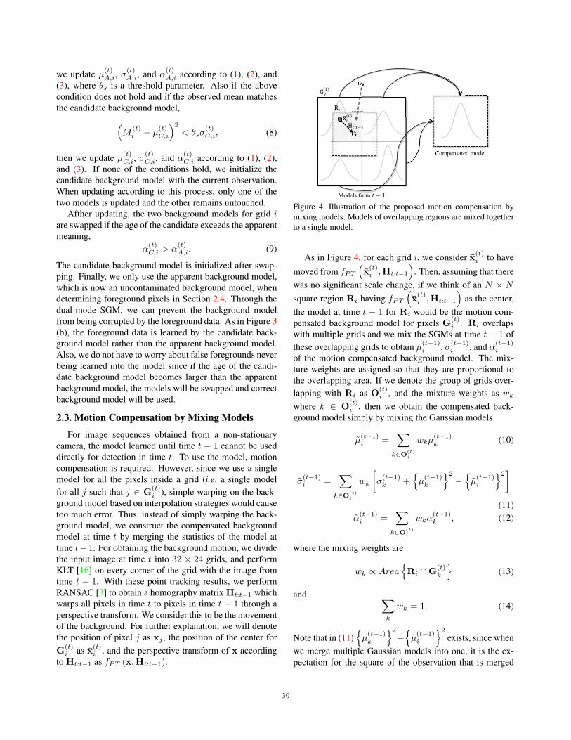
Figure 4. Illustration of the proposed motion compensation by

mixing models. Models of overlapping regions are mixed together

to a single model.

As in Figure 4, for each grid i, we consider x̄(t)i to have

moved from fPT

(x̄(t)i ,Ht:t−1

). Then, assuming that there

was no significant scale change, if we think of an N × N

square region Ri having fPT

(x̄(t)i ,Ht:t−1

)as the center,

the model at time t − 1 for Ri would be the motion com-

pensated background model for pixels G(t)i . Ri overlaps

with multiple grids and we mix the SGMs at time t − 1 of

these overlapping grids to obtain μ̃(t−1)i , σ̃

(t−1)i , and α̃

(t−1)i

of the motion compensated background model. The mix-

ture weights are assigned so that they are proportional to

the overlapping area. If we denote the group of grids over-

lapping with Ri as O(t)i , and the mixture weights as wk

where k ∈ O(t)i , then we obtain the compensated back-

ground model simply by mixing the Gaussian models

μ̃(t−1)i =

∑k∈O(t)

i

wkμ(t−1)k (10)

σ̃(t−1)i =

∑k∈O(t)

i

wk

[σ(t−1)k +

{μ(t−1)k

}2

−{μ̃(t−1)i

}2]

(11)

α̃(t−1)i =

∑k∈O(t)

i

wkα(t−1)k , (12)

where the mixing weights are

wk ∝ Area{Ri ∩G

(t)k

}(13)

and ∑k

wk = 1. (14)

Note that in (11){μ(t−1)k

}2

−{μ̃(t−1)i

}2

exists, since when

we merge multiple Gaussian models into one, it is the ex-

pectation for the square of the observation that is merged

30303030

with weight wk and not the variance itself. During the mix-

ing process, as in Figure 4, models where nearby regions

differ a lot (e.g. edges) will have excessively large variances

after compensation (as in (11)). Normally, a SGM would

not have too large variances, and having such large variance

would mean that the model has not learned much of the tar-

get object. Therefore, after compensation, if the variance is

over a threshold θv , i.e. σ̃(t−1)i > θv , we reduce the age of

the model as

α̃(t−1)i ← α̃

(t−1)i exp

{−λ

(σ̃(t−1)i − θv

)}, (15)

where λ is a decaying parameter. Through this decaying of

age, we prevent the model from having a model with too

large variance. This especially helps removing false fore-

grounds near edges.

2.4. Detection of Foreground Pixels

After obtaining the background model for time t as in

Section 2.1, 2.2, and 2.3, we select pixels that have dis-

tances larger than threshold from the mean as foreground

pixels. This is not an exact solution to the problem the-

oretically, since to be exact, we should find pixels with

lower probability of being the background with respect to

the learned background model. However, finding such pix-

els require much computation, due to the square-root and

natural logarithms operations in the exact equation [15]. We

found empirically that the results are useable even with sim-

ple thresholding with respect to the variance, without com-

plicated computation. Mathematically, for each pixel j in

group i, we classify the pixel as a foreground pixel if

(I(t)j − μ

(t)A,i

)2

> θdσ(t)A,i, (16)

where θd is a threshold parameter. Note that we only use the

apparent background model in determining the foreground.

Through this way, we can avoid false backgrounds arising

from contamination of the background model.

3. ExperimentsFor the experiments, the proposed method was imple-

mented using C++ with the KLT from OpenCV1 library.

For the parameters, the grid size N = 4, the thresh-

old for matching θs = 2, the decaying parameter for age

λ = 0.001, the threshold for decaying age θv = 50 × 50,

and the threshold for determining detection θd = 4. For the

initialization of the variance, we simply set variance to be a

moderate value (e.g. 20× 20). The age was truncated at 30

to keep a minimum learning rate. The method was experi-

mented with eight image sequences, where six is identical

to the sequences used in [8], one is our own, and the last

one is downloaded from YouTube2.

1http://opencv.org/downloads.html2http://www.youtube.com/watch?v=0K4XKTx7T4g

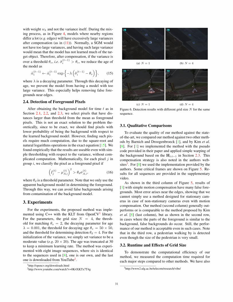
(a) N = 1 (b) N = 4

(c) N = 1 (d) N = 4

Figure 6. Detection results with different grid size N for the same

sequence.

3.1. Qualitative Comparisons

To evaluate the quality of our method against the state-

of-the-art, we compared our method against two other meth-

ods by Barnich and Droogenbroeck [1], and by Kim et al.[8]. For [1] we implemented the method with the pseudo

code provided in their paper and applied simple warping of

the background based on the Ht:t−1 in Section 2.3. This

compensation strategy is also noted in the authors web-

sites3. For [8] we used the implementation provided by the

authors. Some critical frames are shown on Figure 5. Re-

sults for all sequences are provided in the supplementary

video.

As shown in the third column of Figure 5, results of

[1] with simple motion compensation have many false fore-

grounds. Most error arises near the edges, showing that we

cannot simply use a method designed for stationary cam-

eras in case of non-stationary cameras even with motion

compensation. Our method (second column) generally out-

performs or is comparable to the method proposed by Kim

et al. [8] (last column), but as shown in the second row,

in cases where the parts of the foreground is similar to the

background, false backgrounds do occur. Still, the perfor-

mance of our method is acceptable even in such cases. Note

that in the third row, a pedestrian walking by is detected

even though the size of the pedestrian is very small.

3.2. Runtime and Effects of Grid Size

To demonstrate the computational efficiency of our

method, we measured the computation time required for

each major steps compared to other methods. We have also

3http://www2.ulg.ac.be/telecom/research/vibe/

31313131

Figure 5. Comparison results against other methods. Input frames (first column), proposed method (second column), method of Barnich

and Droogenbroeck [1] with simple motion compensation (third column), and method by Kim et al. [8] (fourth column).

Pre-Processing Motion Comp. Modeling Post-Processing Total

Ours with N = 4 and OpenMP 0.82ms 2.00ms 0.88ms - 3.71ms

Ours with N = 4 0.84ms 2.65ms 2.31ms - 5.81ms

Ours with N = 1 0.84ms 18.72ms 6.40ms - 25.96ms

Barnich & Droogenbroeck [1] - 7.20ms 4.15ms - 11.35ms

[1] with our motion compensation - 39.22ms 3.64ms - 42.86ms

Kim et al. [8] 1.15ms 5.90ms 2.32ms 7.85ms 17.23ms

Table 1. Average computation time for each method.

measured our method with parallel processing used (imple-

mented with OpenMP), and in case of N = 1, which means

that all pixels have their own dual-mode SGM. All experi-

ments were performed on an Intel Core i5-3570 3.4GHz PC

with 320×240 image sequences. Table 1 is the average run-

time required for each algorithm. As shown in Table 1, our

method outperforms other methods with respect to compu-

tation load. Even our method with N = 1 runs in average of

25.96ms assuring real-time performance. The computation

time of the method by Barnich and Droogenbroeck [1] is

comparable to our method (11.35ms) but shows relatively

poor performance considering the quality of detection re-

sults (as previously discussed in detail in Section 3.1.) Also,

the influence of the computation load arising from mo-

tion compensation increases when a more precise motion

compensation method, such as our compensation method,

is used rather than simple warping. The method by Kim

et al. [8] also require computation time suitable for real-

32323232

(a) (b)

(c) (d)

Figure 8. Example results when simple nearest neighbor warping

is performed ((a) and (b)) and when the proposed motion compen-

sation by mixing models is performed ((c) and (d)). (a) and (c) are

the means of the apparent background model, and (b) and (d) are

the detection results.

time performance on a PC, but is still computationally ex-

pensive to run on a machine with relatively less computa-

tion power. Furthermore, a simple parallel implementation

with OpenMP reduces the required computation even more,

making our method run in 3.71ms on average. As shown in

Figure 6, the detection performance of our method does not

degrade with respect to N . Rather, false foregrounds arising

from motion compensation errors near edges are reduced.

3.3. Effects of Dual-Mode SGM

As noted in Section 2.2, using one SGM model causes

the background model to be contaminated by the fore-

ground. This causes problems when the scene contains ob-

jects that are relatively large or moving slowly, since they

will contaminate the background significantly and affect the

final detection result. An example of this is shown in Fig-

ure 7. In Figure 7 (a), it can be seen that traces of mov-

ing objects are left in the background model when using

one SGM model, whereas in (b) and (c), with dual-mode

SGM, the traces are learned in the candidate background

model (c) and the apparent background model (b) is pre-

served and clear. As in (d) and (e), this degradation of the

background model decreases the performance of the detec-

tion algorithm.

3.4. Effects of Motion Compensation

Since we use the same dual-mode SGM for multiple pix-

els inside a grid, the motion compensation method proposed

in Section 2.3 plays a critical role for the performance of

the whole algorithm. If we simply apply a nearest neigh-

bor warping to move the pixels, even the SGM model with

age is not able to cope with such compensation errors. Fig-

ure 8 is an example showing the effectiveness of the pro-

posed compensation scheme. In the case of simple nearest

neighbor warping, as shown in (a), the background model

becomes distorted due to quantization effects. This results

in bad detection performance as shown in (b). However,

with the proposed motion compensation scheme, the back-

ground motion is well compensated as in (c). Also, as in

(d), detection performance is unharmed.

3.5. Mobile Results

We have also implemented our method on a mobile de-

vice to further test its real-time capability. The implementa-

tion was done on an Quad-core 1.4 GHz Cortex-A9 android

device with OpenCV for android4 used to implement KLT.

The implementation does not have any optimization tech-

niques used and is basically the same code for PC tweaked

so that it matches the android interface. Our method runs

approximately 20 frames per second with the live capture

resolution set to 160×120. Figure 9 shows actual still shots

of our algorithm running on a mobile device. Although

some small details are not detected due to low resolution,

it is possible to see that our method performs well in real-

time even on a mobile device.

4. ConclusionsA novel method for detecting moving objects in a scene

with non-stationary cameras was proposed. The proposed

method modeled the background through dual-mode SGM

with age to cope with motion compensation errors and to

prevent the background model from being contaminated by

the foreground. A single dual-mode SGM was applied to

multiple pixels to reduce the required computation load,

without performance degradation. To reduce errors arising

from motion compensation, models were mixed together

in the compensation process. Experimental results showed

that our method requires significantly less amount of com-

putation, running within 5.8ms, and yet with robust detec-

tion performances. Also, our method was implemented on

a mobile device, confirming its real-time capability.

AcknowledgementThe research was sponsored by the SNU Brain Korea 21

Information Technology program.

References[1] O. Barnich and M. Van Droogenbroeck. ViBe: A universal

background subtraction algorithm for video sequences. IEEE

4http://opencv.org/platforms/android.html

33333333

(a) (b) (c) (d) (e)

Figure 7. Example result with SGM and dual-mode SGM. (a) mean of the background model for SGM, (b) mean of the apparent background

model of the dual-mode SGM, (c) mean of the candidate background model of the dual-mode SGM, (d) SGM result, and (e) dual-mode

SGM result. The mean of the background model of SGM (a) is contaminated by the foreground, whereas the mean of the apparent

background model of dual-mode SGM (b) remains unharmed. This leads to different results as in (d) and (e).

Figure 9. Example detection results of our method on a mobile device (foreground pixels highlighted in red). Our implementation runs

approximately 20 frames per second, assuring real-time performance.

Transactions on Image Processing, 20(6):1709–1724, June

2011. 2, 5, 6

[2] A. Elgammal, R. Duraiswami, D. Harwood, L. S. Davis,

R. Duraiswami, and D. Harwood. Background and fore-

ground modeling using nonparametric kernel density for vi-

sual surveillance. In Proceedings of the IEEE, pages 1151–

1163, 2002. 1

[3] M. A. Fischler and R. C. Bolles. Random sample consensus:

a paradigm for model fitting with applications to image anal-

ysis and automated cartography. Commun. ACM, 24(6):381–

395, June 1981. 4

[4] G. Georgiadis, A. Ayvaci, and S. Soatto. Actionable saliency

detection: Independent motion detection without indepen-

dent motion estimation. In Proceedings of the IEEE Con-ference on Computer Vision and Pattern Recognition. June

2012. 1

[5] P. KaewTrakulPong and R. Bowden. A real time adaptive

visual surveillance system for tracking low-resolution colour

targets in dynamically changing scenes. Image and VisionComputing, 21(10):913 – 929, 2003. 2

[6] I. Kim, H. Choi, K. Yi, J. Choi, and S. Kong. Intelligent vi-

sual surveillance? survey. International Journal of Control,Automation and Systems, 8(5):926–939, 2010. 1

[7] J. Kim, X. Wang, H. Wang, C. Zhu, and D. Kim. Fast moving

object detection with non-stationary background. Multime-dia Tools and Applications, pages 1–25, 2012. 1

[8] S. Kim, K. Yun, K. Yi, S. Kim, and J. Choi. Detection of

moving objects with a moving camera using non-panoramic

background model. Machine Vision and Applications, pages

1–14. 10.1007/s00138-012-0448-y. 1, 2, 5, 6

[9] T. Ko, S. Soatto, and D. Estrin. Warping background subtrac-

tion. In The Twenty-Third IEEE Conference on Computer

Vision and Pattern Recognition, CVPR 2010, San Francisco,CA, USA, 13-18 June 2010, pages 1331–1338. IEEE, 2010.

1

[10] S. Kwak, T. Lim, W. Nam, B. Han, and J. H. Han. Gener-

alized background subtraction based on hybrid inference by

belief propagation and bayesian filtering. In Computer Vi-sion (ICCV), 2011 IEEE International Conference on, pages

2174 –2181, nov. 2011. 1, 2

[11] A. Mittal and D. Huttenlocher. Scene modeling for wide area

surveillance and image synthesis. In In IEEE Conference onComputer Vision and Pattern Recognition, pages 160–167,

2000. 2

[12] N. I. Rao, H. Di, and G. Xu. Panoramic background model

under free moving camera. In Proceedings of the FourthInternational Conference on Fuzzy Systems and KnowledgeDiscovery - Volume 01, FSKD ’07, pages 639–643, Wash-

ington, DC, USA, 2007. IEEE Computer Society. 2

[13] Y. Sheikh, O. Javed, and T. Kanade. Background subtrac-

tion for freely moving cameras. In ICCV, pages 1219–1225.

IEEE, 2009. 1

[14] Y. Sheikh and M. Shah. Bayesian modeling of dynamic

scenes for object detection. PAMI, 27:1778–1792, 2005. 1

[15] C. Stauffer and W. Grimson. Adaptive background mixture

models for real-time tracking. In Computer Vision and Pat-tern Recognition, 1999. IEEE Computer Society Conferenceon., volume 2, pages 2 vol. (xxiii+637+663), 1999. 1, 3, 5

[16] C. Tomasi and T. Kanade. Detection and tracking of point

features. Technical report, Carnegie Mellon University, Apr.

1991. 2, 4

34343434