HAL Id: halshs-01513123https://halshs.archives-ouvertes.fr/halshs-01513123

Submitted on 24 Apr 2017

HAL is a multi-disciplinary open accessarchive for the deposit and dissemination of sci-entific research documents, whether they are pub-lished or not. The documents may come fromteaching and research institutions in France orabroad, or from public or private research centers.

L’archive ouverte pluridisciplinaire HAL, estdestinée au dépôt et à la diffusion de documentsscientifiques de niveau recherche, publiés ou non,émanant des établissements d’enseignement et derecherche français ou étrangers, des laboratoirespublics ou privés.

Detection of landfill cover damage using geophysicalmethods

Fanny Genelle, Colette Sirieix, Joëlle Riss, Véronique Naudet, StéphaneRenie, Michel Dabas, Philippe Begassat, Fabien Naessens

To cite this version:Fanny Genelle, Colette Sirieix, Joëlle Riss, Véronique Naudet, Stéphane Renie, et al.. Detection oflandfill cover damage using geophysical methods. Near Surface Geophysics, European Association ofGeoscientists and Engineers (EAGE), 2014, 12 (5), pp.599-611. �10.3997/1873-0604.2014018�. �halshs-01513123�

1

DETECTION OF LANDFILL COVER DAMAGES WITH GEOPHYSICAL

METHODS

Fanny GENELLE1,2

, Colette SIRIEIX1, Joëlle RISS

1, Véronique NAUDET

1,3, Stéphane

RENIE2, Michel DABAS

4, Philippe BEGASSAT

5, Fabien NAESSENS

1

1Univ. Bordeaux, I2M, UMR 5295, F-33400 Talence, France ;

2HYDRO INVEST, 514 route d’Agris, 16430 Champniers, France;

3BRGM, 3 avenue Claude Guillemin, 45060 Orléans, France;

4GEOCARTA, 5 rue de la banque, 75002 Paris, France ;

5ADEME, 20 avenue du Grésillé, BP 90406, 49004 Angers cedex 1, France ;

Abstract

On closed landfills, impermeable covers are capping the waste in order to

minimize water infiltration and accumulation of leachate inside the waste. In France, the

cover composition depends notably on the kind of stored waste. In cases of hazardous

waste, the cover must be composed of a drainage layer under the top soil and a

geomembrane or a Geosynthetic Clay Liner (GCL) associated with an underlying 1.0 m

thick low permeability material to ensure its tightness. However, this protection cover is

sometimes damaged leading to an escape of landfill gazes and an unusual increase of

leachate within the waste after rainy events. As leachate treatment is very expensive, it

appears necessary to locate the weakness zones of the cover and assess their sizes in

order to limit maintenance cost on landfills. In order to detect damages in the cover, the

2

following geophysical methods have been carried out on a French landfill: cartography

with an Automatic Resistivity Profiling (ARP©), the Electrical Resistivity Tomography

(ERT) and the Self Potential method (SP). The joint use of these methods has given us

the opportunity to determine the contribution of each of them for cover’s

characterization. The ARP survey has put in evidence the lateral heterogeneity of cover

materials on the whole landfill. The ERT has confirmed the variability of the cover

composition but also provided information about the cover thickness and the damaging

of the GCL. SP measurements have revealed a negative anomaly at the top of the

landfill, possibly linked with a thin and damaged cover and therefore a greater

proximity of waste. Finally, manual augers holes have enabled to associate electrical

resistivity properties with different materials used in the cover and the damaged GCL.

This study on a hazardous waste landfill shows that geophysical methods associated

with manual auger holes have allowed to improve the knowledge of the cover. Thus, the

damaged areas detected thanks to measurements performed on site may be useful for the

landfill manager who can optimize the drilling survey necessary to check the nature of

defects and then choose a suited remediation of the cover.

1. Introduction

Landfills are consisted of several cells filled with waste that are separated from

the underlying soil by a passive security barrier (low permeability clay) associated with

an active barrier (for example a geomembrane). At the end of the waste storage, cells

are protected with a cover so as to minimize infiltration of water into the waste and

therefore reduce the quantity of leachate. In cases of hazardous waste landfills, the

3

cover must contain a geomembrane or a Geosynthetic Clay Liner (GCL) which notably

takes part in the cover impermeability (law of December 18th

1992 published in the

French journal officiel on March 30th

1993). Although ideal barriers would never be

damaged, real covers are often cracked and eroded due to mechanical, climatic and

hydraulic stresses acting on their surface (ageing processes), or even be damaged during

their laying. As leachate treatment is very expensive and proportional to its quantity,

tightness properties of covers must be ensured over time to limit maintenance cost on

landfills. Thus, locating damaged areas is crucial to limit leachate increase within the

landfill, that’s why covers monitoring is a topical subject.

Just after geomembrane installation at the bottom of cells, several electrical

methods have proved their efficiency for checking the geomembrane integrity (Forget et

al. 2005; ASTM D6747). One of these methods consists in applying an electrical

current between one electrode placed above the geomembrane and a second one at a

remote location outside the cells, and then measuring electrical potentials thanks to a

permanent grid of electrodes placed beneath the liner (White and Barker 1997). These

potential measurements can also be performed using the Electrical Leak Imaging

Method (ELIM) thanks to a couple of electrodes moving above the geomembrane,

either in the waste material (Colucci et al. 1999) or in the drainage layer (Laine et al.

1997). Since most synthetic geomembranes are effective electrical insulators, the

presence of a leak creates a localized passage of current, which perturbs the potential

field in a characteristic way. Moreover, the ELIM method can be applied when the

geomembrane takes part in the landfill cap system (Hansen and Beck 2009; Beck 2011).

However, the detection of defects in this latter case is only possible in particular

conditions depending on the nature of the soil and its thickness. All these methods are

4

mainly efficient before waste storage but not in old closed landfills as some electrodes

must be placed in the waste or beneath the liner. Therefore in cases of old landfills,

checking the integrity of covers in a cost and effective way requires to find non invasive

techniques. Thus, the anomalous areas detected by these methods, and possibly linked

with cover damages, would then be checked by a drilling survey performed on these

locations.

As they are non-destructive, geophysical methods can be very interesting tool

for detecting damages in covers. Up to now, these methods have mainly been used to

characterize contaminated plumes (Ogilvy et al. 2002; Naudet et al. 2004; Chambers et

al. 2010; Gallas et al. 2010), or to precise the nature of materials and waste in place

(Guérin et al. 2004; Leroux et al. 2007; Boudreault et al. 2010; Vaudelet et al. 2011).

As leachate is electrically very conductive, it is a suitable target for the electrical

methods especially to monitor leachate recirculation in bioreactor (Grellier et al. 2008;

Clément et al. 2011). To our knowledge, little attention and few published studies have

used geophysical methods to characterize cover on landfills (Carpenter et al. 1991;

Cassiani et al. 2008). Other works have been undertaken on experimental sites in more

controlled conditions to test the feasibility of geophysical methods in the detection of

cover heterogeneities (Guyonnet et al. 2003; Genelle et al. 2011a).

In this study, we attempt to test three geophysical methods on an old hazardous

waste French landfill : the Automatic Resistivity Profiling (ARP©), the Self Potential

(SP) and the Electrical Resistivity Tomography (ERT). These methods have been

previously carried out on an experimental site, which reproduces two kinds of covers

containing heterogeneities incorporated in a controlled fashion (Genelle et al. 2010;

Genelle et al. 2011b). They have been chosen as they are sensitive to several parameters

5

such as lithology (clay content), water content, water flow, and compaction. As the

ARP© system is tracked by a quad, its data acquisition is rapid and therefore interesting

to scan the overall surface of the landfill in a time effective way. Then, the SP and ERT

methods can be used on selected anomalous zones detected by ARP. By combining

these methods, the knowledge of the cover should be improved by locating its possible

damages and assessing their size. Geophysical results should help the site managers to

carry out the necessary drilling survey with the aim of controlling damages, and then to

optimize a suited remediation of the cover (total rebuilding or just on a specific area).

2. Site description and methods

2.1 The landfill

The studied site is an old French hazardous waste landfill settled on a former

clay quarry of lower Permian age. During the exploitation of the landfill, around 400

000 tons of hazardous waste were stored from 1978 to 1988 on a 42 000 square meters

area. Twelve cells were filled by alternate layers of a one meter-thick waste (previously

mixed with clay) and a 0.3 meter-thick clay, leading to a waste dome of around 13 m

height. In 1992, all the cells have been leveled and reshaped to the extent that they were

no more distinguishable from one to each other. After this remodeling phase, an

impermeable barrier covers the entire waste in order to limit vertical water seepage.

Figure 1 presents the theoretical log of the 2.3 m thick cover composed of an alternation

of clayey sand and clay layers. The 7 mm thick Geosynthetic Clay Liner (GCL) is

placed at around 1.1 m deep. A vertical cement-bentonite cutoff wall encloses the

landfill to prevent water entry inside the landfill (Fig. 2). Despite this cover and the

6

wall, the amount of leachate inside the landfill is considered abnormally high after all

rainy events, suggesting water infiltration.

Figure 1 The theoretical cover composition installed in 1992 on the French hazardous waste

landfill.

Manual auger hole

SP measurements

a)

Cement-bentonite cutoff wall

ERT profile

Supposed waste storage area

Leachate convergence well

Leachate drains

A

B

Track

b)

Manual auger hole

7

Figure 2 a) Map of the landfill with topographic lines and location of geophysical

measurements b) Topography along the ERT profile named AB with location of manual auger

holes

2.2 Geophysical methods

The Automatic Resistivity Profiling (ARP©) system uses a patented multi-electrode

device connected to wheel-based electrodes which roll over the ground surface (Dabas

2009). The rolling electrodes are arranged in a trapezoid pattern. Electrical current is

injected into the ground by a pair of electrodes and resistance is measured by three other

pairs of electrodes acting as potential dipoles (Fig. 3). The different electrode spacings

between injection dipole and potential ones (respectively 0.5, 1.0 and 2.0 m) allow

simultaneous acquisition of apparent electrical resistivity data at three increasing

investigation depths.

Figure 3 Sketch of electrodes configuration used in the ARP system. C1 and C2 are

current injection electrodes, P1 and P2, P’1 and P’2 P’’1 and P’’2 are potential

measurements electrodes.

The system includes a differential GPS and is towed by a quad bike for quicker data

acquisition. Site coverage follows a grid of parallel survey lines in a bi-directional

8

pattern, guided by on-board navigation. Data is plotted as apparent resistivity maps for

each channel. The ARP© system (Dabas 2009) is already used in archeological surveys

(Papadopoulos et al. 2009; Campana and Dabas 2011), viticultural farming (Costantini

et al. 2009; Ghinassi et al. 2010) and geology in an alluvial landscape (Tye et al. 2011).

Because of its speed of data acquisition it would seem to be interesting to carry out it on

landfills.

ARP measurements were performed in November 2009 on the overall landfill

with a 1 m line spacing. The survey lasted about six hours, with a speed quad of 10 km

per hour and a measurement each 0.1 m. Data processing involved a spline interpolation

on a 0.5 m regular mesh.

The Self-Potential (SP) method consists in measuring the natural electrical

potential at the ground surface. The SP signals are associated with different polarization

mechanisms occurring naturally in the ground (e.g. Jouniaux et al. 2009). The main

sources are due to water fluxes in the vadose zone (Thony et al. 1997; Doussan et al.

2002; Linde et al. 2011) and/or saturated zone (Rizzo et al. 2004; Maineult et al. 2008;

Bolève et al. 2009) through the electrokinetic coupling, gradients in chemical potential

through the electrochemical coupling and redox processes (Maineult et al. 2004; Naudet

and Revil 2005). These sources constitute the primary sources of the SP signals. The

secondary sources are due to electrical resistivity contrasts of the subsurface. Therefore,

a detailed knowledge of the electrical resistivity distribution is necessary to accurately

modelize SP responses. The multiplicity of sources mirrors the main limitation of the

SP method as many different processes contribute to the measured response. In this

study, we expect to detect three main sources : electrokinetic effect and electrical

9

contrasts in zones where cracks in the cover facilitate surface water infiltration, and

oxido-reduction reactions due to waste biodegradation.

The equipment used for the measurement were a MX20 Metrix voltmeter with a high

input impedance (~108 Ω), one cable reel and two non-polarisable Pb/PbCl2 electrodes

(Petiau 2000). The SP survey was carried out just after ARP measurements and was

focused on the area delimited by the black rectangle, characterized by a high electrical

resistivity contrast on the slope (Fig. 5). Measurements were performed between a

roving electrode and a fixed electrode at a base station. The measurement mesh was 5 m

square with profiles oriented from West North-West to East South-East. To ensure

uniform ground contact between the electrodes, small holes were dug at each station and

filled with bentonite mud. The SP signal at each measurement point was stable, the

maximum variation was estimated at more or less 1 mV. During the mapping, several

SP measurements were performed with the two electrodes placed in the base station

hole in order to make a linear drift correction of the data.

The Electrical Resistivity Tomography (ERT) is based on the injection of

electrical current into the ground followed by the measurement of resulting potential

differences between a set of electrodes. This method has already been used to locate

seepage or erosion in dams (Johansson and Dahlin 1996; Sjödhal et al. 2008) or to map

landfill geometry (Reynolds and Taylor 1996; Bernstone and Dahlin 1997). The ERT

applications has been also applied to estimate the soil water content (Michot et al. 2003;

Schwartz et al. 2008; Brunet et al. 2010) or to characterize the soil heterogeneity

(Samouëlian et al. 2003; Besson et al. 2004) and its compaction (Abu-Hassanein et al.

1996).

10

As it is time-consuming to perform ERT measurements on the whole cover of the

landfill, a specific zone observed with the ARP was selected to carry out the ERT

profile (see location on Fig. 2). Measurements were performed in June 2010 thanks to

72 electrodes installed every 0.5 m connected to a Syscal Pro resistivimeter. Different

arrays, defined according to measurements formerly carried out on an experimental site,

were at first implemented on a test panel in order to choose the appropriate acquisition

parameters. Since the dipole-dipole array has given good results on the experimental

site (Genelle et al. 2011b), especially in the detection of a 0.1 m wide crack by a

pronounced electrical contrast with the surrounding gravelly-clay material, it was

consequently used on this site with a roll-along technique (24 electrodes overlap

between each panel). In order to reach the waste depth and knowing that the theoretical

thickness of the cover is 2.3 m, measurements were performed using two different

sequences on the AB profile without moving electrodes : the first sequence with a

distance between potential electrodes “a” equals to 0.5 m and the second one with a

distance “a” equals to 1.0 m (Fig. 4). These two sequences provide data until

investigation depths of 2.3 and 5.7 m respectively.

Figure 4 Sketch of electrodes configuration for dipole-dipole array used for the ERT

measurements. C1 and C2 are current injection electrodes, P1 and P2 are potential

measurements electrodes.

Data inversion was carried out with the RES2DINV software (Loke 2010) using

2D regularized least square optimization method with robust (L1-norm) model

constraints inversion (Loke et al. 2003) combined with a model refinement. Due to a

high electrical resistivity contrasts on site, the L1-norm was more adapted as it produces

11

a more accurate resistivity pattern with sharper boundaries than with the smoothness

constrained L2-norm.

2.3 Manual auger holes

Sixteen manual auger holes were dug along the ERT profile in order to improve

the knowledge of the cover in this part of the landfill (Fig. 2). The description of the

cover materials was done macroscopically and their lithology chosen according to the

more or less ratio of sand and clay estimated qualitatively with the help of experienced

geologists. The GCL condition (undamaged or not) was put in connection with the more

or less resistance of the manual auger. As the GCL is known to be mechanically very

resistant, when it was crossed without any resistance, the GCL was defined as “very

damaged” and most of the time the presence of textile fibers or bentonite was observed

in samples extracted from the auger. When it was not crossed, we assumed that it was in

“good” condition e.g. less damaged.

3. Results

ARP measurements

The three maps obtained with the 0.5, 1.0 and 2.0 m electrode spacing (Fig. 5)

show apparent electrical resistivity variations between 10 and 200 Ω.m. The spatial

layout of electrical resistivities can be divided into four areas which differently behave.

The first area, located in the north part of the landfill, gathers high electrical resistivities

12

(more than 70 Ω.m) whatever the electrode spacing. The second area, focused on the

south part of the landfill, brings together all the places where apparent electrical

resistivity decreases with the electrode spacing. This behavior may be linked with the

theoretical cover composed of sandy materials upon clayey ones (Fig. 1).

The third area shows low resistivities (<40 Ω.m) on the 0.5 m electrode spacing,

resistivities that tend to decrease with the increasing investigation depth. It could result,

among a lot of other causes, from the presence of a higher clay content in the shallow

cover materials. Finally, the fourth area is pinpointed on the north and the east

boundaries of the landfill in a thin and straight area where electrical resistivity values

are the lowest with the three electrode spacings. Their delimitation corresponds to the

zone between leachate drains and the cutoff wall (Fig. 2). Thus, this saturated area at the

foot of slope, outside the waste cells, can be due to the concentration of water fallen

during the seven days before the survey (accumulation equals to 19 mm).

These observations underline the heterogeneity of the cover that can be either due to the

materials itself (more or less clayey materials) or to variation of compaction, water

content, weathering, lithology and a more or less damaged GCL.

The area delimited by the black rectangle on Figure 5, where a high apparent electrical

resistivity contrast can be seen on the slope, is the zone where SP measurements were

performed in order to improve the knowledge of the cover in this part of the landfill.

13

a) 0.5 m electrode spacing b) 1.0 m electrode spacing c) 2.0 m electrode spacing

Apparent electrical resistivity (Ω.m)

Figure 5 The three apparent electrical resistivity maps obtained with the ARP with the 0.5 m electrode spacing (a), the 1.0 m electrode spacing (b) and

the 2.0 m electrode spacing (c). The SP measurement area is delimited by the black rectangle. The location of leachate drains are represented by white

lines.

N N N 20 m 20 m 20 m

10 30 50 70 100 150 200

14

SP measurements

Figure 6 displays the five SP profiles oriented East South-East to West North-

West on the black rectangle seen on Figure 5. The SP signal ranges from -81 to +42

mV, with a similar behavior on each profile. Based on the signal dynamic, three

different zones have been defined. Zone A, at the foot of the landfill, is marked by

positive SP values (from +2 and +42 mV). Zone B is characterized by a rather stable

signal with about 70 % of values contained between -10 and +10 mV. Zone C, located

at the top of the landfill, shows a sharp decrease of SP signal (until -81 mV on the

profile y=5 m) followed by an increase of SP.

Figure 6 a) East South-East to West NorthWest profiles b) Location of the SP profiles (black

lines) and the ERT profile (red line AB)

Since measurements along the profile y=5 m show the most variation of SP signal, an

ERT profile was performed on the same location.

a)

b)

Zone A Zone B Zone C E.SE W.NW

E.SE

W.NW A

B

15

ERT measurements

The two ERT profiles (measurements acquired with a=0.5 m and a=1.0 m) highlight

electrical resistivity variations between 0.5 and 400 Ω.m, not only laterally but also

vertically (Fig. 7). The deeper model resistivity ERTa clearly shows the presence of low

resistivity values (<4 Ω.m symbolized by grey color) at each end of the profile

(respectively at about -2.3 and -1.3 m deep). These low electrical resistivity values

would indicate the occurrence of waste, closer to the surface at the top of the landfill

where the cover thickness is thinner than the theoretical one (Fig. 1). On the central part

of the model resistivity, the waste are not seen on the model resistivity and appears to be

deeper.

The two model resistivity display a different spatial layout of electrical resisitivity

above waste, particularly between 5 and 25 m of the origin of the profile : the model

resisitivity ERTa displays two cover layers (Fig. 7 a) whereas the ERTb shows three

layers (Fig. 7 b). Moreover, the waste depth is lower on the model resistivity ERTb than

on the ERTa. The waste depth estimated on the ERTb is more in accordance with the

auger holes dug along the AB profile. However, we can note that it exist a small

difference (less than 10%) between the waste depth estimated on ERTb and their real

depth at the location of the most part of the auger holes. It is probably related to the

thickness inversion model blocks.

The central zone (between 30 and 90 m) displays the highest electrical resistivity values

from 1 to 2 m deep, especially between 32 and 60 m (140<ρ<450 Ω.m). According to

the theoretical log of the cover (Fig. 1), these values would be the signature of the GCL,

which is normally present at a 1.1 m depth over the whole landfill and then should be

observed on the entire profile. Nevertheless, measurements performed on the

16

experimental site (Genelle et al. 2011a) on a cover made of an undamaged and

unsaturated GCL (6 mm thick) have shown very high electrical resistivity values (~4000

Ω.m) associated with an overestimated thickness (over 1 m) on the model resistivity.

That’s why we assume that lower electrical resistivity values (ρ<140 Ω.m) observed on

site should be explained by a saturated and/or damaged GCL. In order to check this

hypothesis, manual auger holes and forward modeling have been made.

Figure 7 Model resistivity of the ERT profile and location of manual auger holes

a) ERTa : dipole-dipole array obtained with a=1.0 m (investigation depth = 5.7 m; Iteration 5 –

Abs error= 1.80 %) b) ERTb : dipole-dipole array obtained with a =0.5 m (investigation depth

= 2.3 m; Iteration 5 – Abs error= 0.94 %).

17

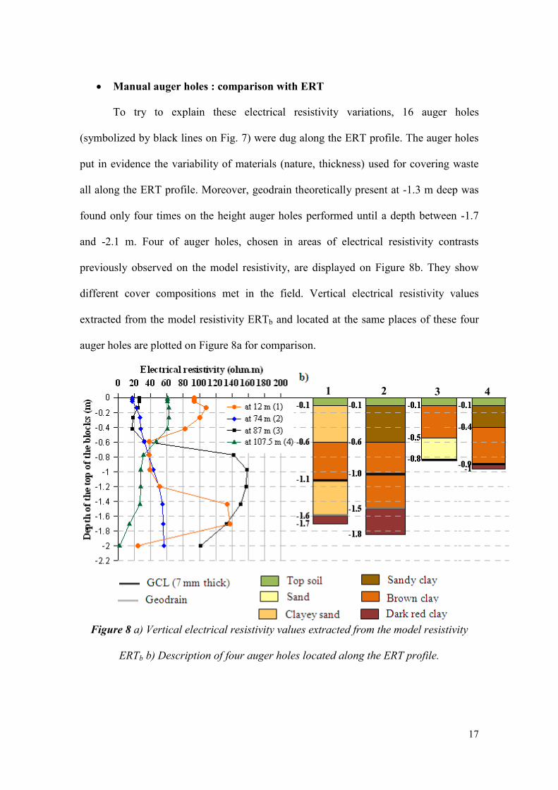
Manual auger holes : comparison with ERT

To try to explain these electrical resistivity variations, 16 auger holes

(symbolized by black lines on Fig. 7) were dug along the ERT profile. The auger holes

put in evidence the variability of materials (nature, thickness) used for covering waste

all along the ERT profile. Moreover, geodrain theoretically present at -1.3 m deep was

found only four times on the height auger holes performed until a depth between -1.7

and -2.1 m. Four of auger holes, chosen in areas of electrical resistivity contrasts

previously observed on the model resistivity, are displayed on Figure 8b. They show

different cover compositions met in the field. Vertical electrical resistivity values

extracted from the model resistivity ERTb and located at the same places of these four

auger holes are plotted on Figure 8a for comparison.

Figure 8 a) Vertical electrical resistivity values extracted from the model resistivity

ERTb b) Description of four auger holes located along the ERT profile.

1 2 3 4

18

At first, one can see that at the location of the three auger holes for which the

GCL was crossed (1, 2, 4), the thickness cover is smaller than the theoretical one

because waste mixed with dark red clay were found at about -1.6 m deep at 12 m (1), at

-1.5 m deep at 74 m (2) and only at -1 m deep at 107.5 m (4) whereas they should be

reached from 2.3 m deep (Fig. 1). Then, the material just above the GCL identified as

brown clay at these three auger holes, whereas it was sand at 87 m (3), is well

characterized by an electrical resistivity of about 35 Ω.m on the vertical profiles.

Different lithology exist in the upper part of the cover : clayey sand at 12 m is

characterized by high electrical resistivity (ρ ~100 Ω.m), sandy clay at 74 and 107.5 m

by a resistivity all the more so low that the sand content is small in the material (here

values between 20 and 60 Ω.m) and brown clay at 87 m. Even if the nature of materials

above the GCL is not the same on these four auger holes, we can note that the thickness

of the two first cover layers is close to the theoretical one, with a GCL in the right place.

The main difference between the four auger holes occurs at the GCL’s depth, between -

0.8 and -1.1 m deep : electrical resistivity increases until 160 Ω.m at 87 m from -1.6 m

deep and 140 Ω.m at 12 m from -1.2 m deep. At the two other places, electrical

resistivity at these depths remains lower than 60 Ω.m.

To explain these different behaviors, we have computed several forward

modelings with RES2MOD. As the cover composition at the auger hole located at 12 m

is the closest to the theoretical one, we have reproduced it using the electrical resistivity

variations met at this location (Tab. 1). Several cases have been studied but here we

present only two of them that are considered to be the most representative. A first

modeling was created with an unsaturated and undamaged GCL (ρ=8400 Ω.m and 0.1

m thick) that corresponds to a value of at least 120 000 Ω.m measured on laboratory on

19

a 7 mm thick undamaged GCL (in applying the equivalence principle). A second

modeling was made with a more saturated and torn GCL (ρ=840 Ω.m and 0.1 m thick).

Thickness layers (m) Forward modeling 1 Forward modeling 2

0 – 0.6 Clay sand ( 102 Ω.m)

0.6 – 1.1 Clay (33 Ω.m)

1.1 – 1.2 GCL (8400 Ω.m)

Equivalent to 120 000 Ω.m

for 7 mm thick

GCL (840 Ω.m)

Equivalent to 12 000 Ω.m

for 7 mm thick

1.2 – 1.6 Saturated clay sand (50 Ω.m)

>1.6 Waste (4 Ω.m)

Table 1 Electrical resistivity and thickness of cover materials layers chosen for forward

modelings.

In order to compare at best the data of these two forward modelings with the

measurements on site along the ERT profile, they have been inverted using the same

kind of inversion, that is to say robust model constraints combined with a model

refinement (Fig. 9).

Electrical resistivity (Ω.m)

Figure 9 a) Model resistivity resulted from the inversion of the forward modeling 1

(with an undamaged and unsaturated GCL) b) Model resistivity resulted from the inversion of

the forward modeling 2 (with a saturated GCL and a 0.125 m wide tear at the vertical of 14 m).

Both the model resistivity resulted from the inversion of the forward modelings show an

overestimated thickness of the GCL from -1.1 m deep. In the case of the undamaged

a)

b)

20

GCL, electrical resistivities are higher than 200 Ω.m (Fig. 9 a). These values have been

observed on the central part of the model resistivity (until 450 Ω.m). In the case of the

more saturated GCL, electrical resistivities are about 100 Ω.m (Fig. 9 b). Moreover, a

decrease of resistivity (ρ~80 Ω.m) is seen at the GCL’s depth at the vertical of 14 m, at

the place of the tear previously created. Furthermore, we can note that low resistivities

are seen in deep even in the part where the GCL was not torn. They are linked with the

materials present below the GCL.

These modeling let us link the electrical resistivity variations previously seen on the

model resistivity at the GCL’s depth with its damaging condition, especially at the

location of the three auger holes 1,2 and 4 described on Figure 8. Thus, on the one hand,

the lack of high electrical resistivity from the GCL’s depth at the auger holes 2 and 4

means that the GCL is damaged and/or saturated. On the other hand, electrical

resistivities reaches 120 Ω.m at the auger hole 1 and seems to be representative of a less

damaged and/or saturated GCL.

Finally, the variation of electrical resistivity seen on the model resistivity ERTb (a=0.5

m) until the GCL’s depth can be related to different nature of cover materials for all the

manual auger holes. Moreover, the use of forward modeling has demonstrated the link

of electrical resistivity variations at -1.1 m depth with the damaging condition of the

GCL.

4. Discussion

In this part, we have compared more particularly the ARP and ERT

measurements in order to know if similarities exist between them. Then, we have

21

studied together the measurements acquired by the three geophysical methods (ARP,

ERT and SP) along the AB profile.

Even if the geophysical methods were not carried out simultaneously on the

landfill, we attempt to compare in a first time apparent electrical resistivities obtained

with the ARP and the ERT along the AB profile (Fig. 10) thanks to statistical methods.

Figure 10 a) Apparent electrical resistivity extracted from ARP measurements along

the AB profile b) Apparent electrical resistivity pseudosection of the ERTb profile

(dipole-dipole array obtained with a=0.5 m).

The apparent electrical resistivity provided by the ARP survey displays similar

variations along the AB profile whatever the electrode spacing (Fig. 10 a) : values are

globally higher than 80 Ω.m from the beginning of the profile to 60 m while they are

lower than 60 Ω.m in the second part of the profile. The apparent electrical resistivity

22

obtained with the ERT shows globally the same resistivity range on the shallow part of

the pseudosection. The values in the deep part of the pseudosection (from about 1.0 m

deep) are lower than these seen on the ARP 2.0 m electrode spacing, especially at each

end of the profile.

On the most part of the profile, ARP apparent electrical resistivity tends to decrease

with the increasing electrode spacing. For example, at 12 m the electrical resistivity

respectively equals to 122 Ω.m and 82 Ω.m for the ARP 0.5 and 2.0 m electrode

spacings. An opposite behavior can be seen between 65 and 90 m : apparent electrical

resistivity are higher with the ARP 2.0 m electrode spacing, about 60 Ω.m compared to

40 Ω.m with the two others electrode spacings. On the pseudosection, electrical

contrasts between the shallow material and the underlying one is more pronounced : at

12 m, resistivities decrease from 150 to 40 Ω.m with depth whereas, in the area between

65 and 90 m, they are contained between 15 and 40 Ω.m. These two different vertical

variations of apparent electrical resistivity can be linked with the variability of cover

materials. For instance, the shallow material at 74 m is characterized by higher clay

content than it is at the same depth at 12 m (Fig. 8). The lowest apparent electrical

resistivity values (<60 Ω.m) on the ARP 2.0 m electrode spacing are focused at the end

of the profile where the cover is thin. In this zone, the pseudosection also shows lower

apparent electrical resistivity with increasing depth, in connection with the influence of

waste.

In order to investigate relationships between ARP and ERT data, we have

computed the Pearson correlation coefficient for all pairs of the twenty-three variables

corresponding to the resistivity acquired with the three ARP devices (electrode spacing

0.5, 1.0 and 2.0 m - Fig. 3) and the twenty configurations characterized by a different

23

distance L of the dipole-dipole array (ERT) (Fig. 4). This correlation matrix has been

calculated for a set of 23 per 29 values of resistivity sampled each 5 m between -15 and

125 m along the AB profile (Tab. 2).

N° variable 1 2 3 4 5 6 7-21 22 23

Variable ARP

(0.5)

ARP

(1.0)

ARP

(2.0)

ERT

(1.5)

ERT

(2.0)

ERT

(2.5) …

ERT

(9.0)

ERT

(9.5)

ARP (0.5) 1.00 0.98 0.74 0.84 0.84 0.76 … … -0.04 -0.04

ARP (1.0) 0.98 1.00 0.80 0.79 0.80 0.75 … … 0.06 0.07

ARP (2.0) 0.74 0.80 1.00 0.49 0.52 0.55 … … 0.52 0.53

ERT (1.5) 0.84 0.79 0.49 1.00 0.92 0.75 … … -0.20 -0.20

ERT (2.0) 0.84 0.80 0.52 0.92 1.00 0.86 … … -0.26 -0.26

ERT (2.5) 0.76 0.75 0.55 0.75 0.86 1.00 … … -0.25 -0.25

… … … … … … … 1.00 … 0.02 0.01

… … … … … … … 1.00 0.99 0.98

ERT (9.0) -0.04 0.06 0.52 -0.20 -0.26 -0.25 0.02 0.99 1.00 0.99

ERT (9.5) -0.04 0.07 0.53 -0.20 -0.26 -0.25 0.01 0.98 0.99 1.00

Table 2 Correlation matrix computed between apparent electrical resistivity obtained

with the ARP and the ERT.

The correlation coefficient is a measurement of how two variables are related. High

positive values indicate possible relations among pairs of variables. We can see in

particular that the highest correlation for the ARP (0.5) and ARP (1.0) is found with the

L=2.0 m configuration of the dipole-dipole array. Focusing our attention on the possible

relation among ARP resistivity variable and ERT resistivity variable (Tab. 3), the

highest correlation (r=0.87) is found for the L=4.0 m configuration of the dipole-dipole

array and ARP (2.0). It means that 76 % (r²=0.87²) of the variability of the ERT

resistivity is accounted by ARP (2.0) resistivity. Moreover, testing the null hypothesis

H0 that the two variables are independent, shows that the null hypothesis should not be

accepted, at a very high significant level (α<0.001). A strictly similar conclusion arises

when computing the Kendall non parametric rank correlation as it has already been

24

done for geophysical purposes by Gebbers et al. (2009) : the null hypothesis is

respected with a statistically highly significant level (p value<0.001).

ARP

(0.5)

ERT

(1.5)

ERT

(2.0)

ERT

(2.5)

ERT

(3.5)

ERT

(4.0)

ARP (0.5) 1.00 0.84 0.84 0.76 0.67 0.57

ARP (1.0) 0.98 0.79 0.80 0.75 0.72 0.65

ARP (2.0) 0.74 0.49 0.52 0.55 0.81 0.87

ERT (1.5) 0.84 1.00 0.92 0.75 0.46 0.40

Table 3 Extract of the correlation matrix computed between apparent electrical

resistivity obtained with the ARP and the ERT.

Table 2 and Table 3 show Pearson coefficients relating ARP and ERT measurements

from the studied area; they should not be considered as universal. Nevertheless, in the

present case, the ARP (2.0) is effectively the most correlated with the L=4.0 m

configuration of the dipole-dipole array of the ERT that corresponds to a pseudodepth

of about 0.87 m (Edwards 1977). This pseudodepth of investigation is defined as the

depth where the earth above it has the same influence on the measured potential as the

lower part. According to these results, we could conclude that ARP 2.0 m electrode

spacing is not able to detect the GCL present at a 1.1 m depth, knowing that the Edward

pseudodepth of investigation has been defined for homogeneous grounds although it is

not the case in our study. Dabas et al. (2009) studied, in the case of two-layers, the

depth from which the presence of a layer is not anymore detectable. Taking a

detectability threshold of 10 %, they showed that the ARP (2.2) could be able to detect a

resistive layer whose top is located between 2 and 3 m depth when the resistivity

contrast with the upper conductive layer varies between 2 and 12. In this study, layers

are still considered as homogeneous. It appears actually in our site (Fig. 10) that ARP

(2.0) could detect the effect of a resistive layer between 60 and 90 m. However, it is not

the case between 35 and 60 m where a resistive layer has been put in evidence by TRE.

We outline here the difficulty in only observing apparent electrical resistivity maps

25

faced with very heterogeneous shallow fields. It confirms that the ARP is mainly

influenced by the cover materials close to the surface and does not reach the GCL.

After the previous comparison between apparent electrical resistivity acquired with

ARP and ERT, we have analyzed together the measurements acquired by the three

geophysical methods (ARP, ERT and SP) along the AB profile.

To facilitate the comparison of these methods between 10 and 120 m along the AB

profile, electrical resistivity values were regularly sampled from the model resistivity

ERTb between -1.4 and -2.0 m and apparent electrical resistivity values from the 2.0 m

electrode spacing of the ARP, and then were plotted with the SP values of the y=5 m

profile (Fig. 11). The depths of blocks chosen for the electrical resistivity values are

these characterizing at best the GCL (Fig. 8).

26

Figure 11 Comparison of the three geoelectrical methods a) Profiles showing electrical

resistivity values extracted from the model resistivity ERTb (obtained with a =0.5 m) at two

different depths, apparent electrical resistivity values extracted from the 2.0 m electrode

spacing of the ARP, and SP profile y=5 m b) Model resistivity ERTb of the AB profile.

The beginning of the profile shows a decrease of SP signal from +40 to +10 mV while

ARP and ERT values, lower than 140 Ω.m, do not reveal high variations of resistivity.

On the central part of the profile (between 30 and 90 m), electrical resistivity between -

1.4 and -2.0 m are contained between 80 and 140 Ω.m (with high values focused from

27

30 to 60 m). A similar variation of apparent electrical resistivity is observed on the ARP

values. In this area, the GCL seems to be in better condition and could prevent SP signal

from going through it. This assumption could explain the relative stability of the SP

signal (variations from -10 to +10 mV) in this part of the profile.

The end of the profile (Fig. 11) displays a decrease of electrical resistivity until 3 Ω.m

from -1.7 to -2.0 m : the waste depth, checked by manual auger holes is really closer to

the surface at the top of the landfill. The apparent electrical resistivity of the 2.0 m

electrode spacing also tends to decrease but only from 110 m and weakly. The SP signal

also shows a great anomaly of around -70 mV at the top of the landfill. We can assume

that this negative SP anomaly can be mainly associated with the shallow presence of

biodegradation waste that are known to produce a strong negative SP signal (Naudet

and Revil 2005; Arora et al. 2007). Moreover, a correlation matrix, made on the

electrical resistivity (ERT, ARP) and SP, has highlighted that the maximum correlation

of SP signal, equals to 0.40, is obtained with the ARP 2.0 m electrode spacing. Given

that electrical resistivities of the ARP (2.0 m) and the ERT (L=4.0 m) are correlated to

each other (r=0.87) whereas they are not to the SP, we can conclude that the physical

phenomena influencing each method are in a certain way independent.

Finally, the high apparent electrical resistivity contrasts seen with the ARP 0.5 and 1.0

m electrode spacing, due to the very heterogeneous nature of cover materials, lead in a

certain way to a difficult detection of the GCL with the ARP (2.0). An inversion of the

ARP data would be necessary to have accurate information about the cover. Moreover,

a bigger electrode spacing would allow to increase the ARP investigation depth. Finally,

the ERT is not only sensitive to the nature of materials (especially the clay content) but

28

also to the GCL’s condition (damaged, saturated or not) and the waste depth located

between -1.6 and -0.9 m along the AB profile.

5. Conclusion

Three geophysical methods, the Electrical Resistivity Tomography (ERT), the

Automatic Resistivity Profiling (ARP©) and the Self Potential (SP), have been applied

on a French hazardous waste landfill in order to determine their ability to detect

damages in the cover. Knowledge of the defect location is important because they can

induce preferential water pathways and unusual increase of leachate within the waste

mass.

ARP and ERT (with a=1.0 m) have together enabled to discover numerous

heterogeneities unsuspected given the knowledge of the theoretical log of the cover. The

ARP has highlighted lateral variations of cover materials on the overall landfill thanks

to maps obtained at three different investigation depths. Apparent electrical resistivity

variations have been shown to mainly correspond to different lithologies in the shallow

cover materials. These high electrical contrasts in the shallow part of the cover have in a

certain way prevented the detection of deeper variations at the GCL’s depth. That’s why

the only use of the ARP is not up to date sufficient to fully understand the cover

behavior because of a too much limited number of investigation depths in available

instrumentation. Ideally, the addition of potential dipoles with several electrode

spacings on the actual configuration of the ARP would allow to inverse all the data,

providing a more reliable result.

A more detailed analysis performed with the ERT with a 0.5 m electrode spacing

in spite of 1.0 m has allowed to detect fine lateral and vertical changes in the cover. The

29

use of two measurements sequences along the same profile has allowed us to notice

differences in the resulting model resistivity. The presence of three different layers

(between 5 and 25 m of the origin of the AB profile) on the model resistivity with a=0.5

m has been observed whereas they are only two on the model resistivity with a=1.0 m

for which the third layer between 1.1 and 1.8 m deep has not been identified. As the

cover composition displays on the 0.5 m model resistivity is in agreement with the

materials met at the manual auger holes, we realize that the inversion taking account

very low resistivities (waste) provides a biased model resistivity. That’s why it appears

necessary to inverse data without the bottom conductive levels (ρ<10 Ω.m)

corresponding to the waste in order to have a more realistic image of the cover.

The ERT has also put in evidence the existence of high electrical resistivity

variations at the GCL’s depth (-1.1 m deep). Low electrical resistivities (ρ<140 Ω.m)

displayed on the model resistivity correspond to a GCL characterized by a value of

12 000 Ω.m thanks to forward modeling. It means that in this case the GCL is damaged

and/or saturated because electrical resistivities reach about 4000 Ω.m on the model

resistivity in the case of an undamaged and less saturated GCL defined by a value of at

least 120 000 Ω.m for a 7 mm thickness.

The variability of the damaging condition of the GCL has an influence on the estimation

of the waste depth on the model resistivity. Thus, when the GCL is the most resistive,

the waste depth on the model resistivity is overestimated in comparison to the reality.

On the contrary, when the GCL is damaged, the waste depth estimated on the 0.5 m

model resistivity is close to the depth found with manual auger holes. In this case, a

small difference (less than 10 %) has been noticed between the estimated and real

depths.

30

SP measurements have revealed a sharp negative anomaly observed at the top of

the landfill that seems to be linked with the presence of waste shallower that somewhere

else.

Based on these results, the area located at the top of the landfill characterized by a

cover with a damaged and/or saturated GCL and the presence of waste near to the

surface could be considered as a preferential water infiltration zone. Numerous defects

have also been noticed along the ERT profile, linked more particularly with low

resistivity at the GCL’s depth.

This study has shown the contribution brought by the geophysical methods to

improve the knowledge of the cover. Use these non-destructive tools associated with

manual auger holes can help the site managers to optimize a suited remediation of the

cover (total rebuilding or just on a specific area).

References

Abu-Hassanein Z.S., Benson C.H. and Blotz L.R. 1996. Electrical resistivity of

compacted clays. Journal of Geotechnical Engineering 122, 397-406.

Arora T., Linde L., Revil A. and Castermant J. 2007. Non-intrusive characterization of

the redox potential of landfill leachate plumes from self-potential data. Journal

of Contaminant Hydology 92, 274-292.

ASTM D6747. Standard Guide for Selection of Techniques for Electrical Detection of

Potential Leak Paths in Geomembranes.

31

Beck A. 2011. Technical improvements in Dipole Geoelectric Survey Methods.

Symposium on geosynthetics (GEOFRONTIERS), Dallas, USA.

doi: 10.1061/41165(397)290.

Bernstone C., Dahlin T., Ohlsson T. and Hogland W. 2000. DC-resistivity mapping of

internal landfill structures: two pre-excavation surveys. Environmental

Geology 39, 360–371.

Besson A., Cousin I., Samouëlian A., Boizard H. and Richard G. 2004. Structural

heterogeneity of the soil tilled layer as characterized by 2D electrical resistivity

surveying. Soil and Tillage Research, 239-249.

Bolève A., Revil A., Janod F., Mattiuzzo J.L. and Fry J.-J. 2009. Preferential fluid flow

pathways in embankment dams imaged by self-potential tomography. Near

Surface Geophysics, 447-462.

Boudreault J.P., Dube J.S., Chouteau M., Winiarski T. and Hardy, E. 2010. Geophysical

characterization of contaminated urban fills. Engineering Geology 116, 196-206.

Brunet P., Clément R. and Bouvier C. 2010. Monitoring soil water content and deficit

using Electrical Resistivity Tomography (ERT) – A case study in the Cevennes

area, France. Journal of Hydrology 380, 146-153.

Campana S. and Dabas D. 2011. Archeological Impact Assessment : The BREBEMI

Project (Italy). Archeological Prospection 18, 139-148.

Carpenter P.J., Calkin S.F. and Kaufmann R.S. 1991. Assessing a fractured landfill

cover using electrical resisitivty and seismic refraction techniques. Geophysics

56, 1896-1904.

32

Cassiani G., Fusi N., Susanni D. and Deiana R. 2008. Vertical radar profiling for the

assessment of landfill capping effectiveness. Near Surface Geophysics 6, 133-

142.

Chambers J.E., Kuras O., Meldrum P.I., Ogilvy R.D. and Hollands J. 2002. Electrical

resistivity tomography applied to geologic, hydrogeologic, and engineering

investigations at a former waste-disposal site. Geophysics 71, 231–239.

Clément R., Oxarango L. and Descloitres M. 2011. Contribution of 3-D time-lapse ERT

to the study of leachate recirculation in a landfill. Waste Management 31, 457-

467.

Colucci P., Darilek G.T., Laine D.L. and Binley A. 1999. Locating landfill leaks

covered with waste. Symposium on Waste Management and Landfill, Cagliari,

Italy.

Costantini E.A.C., Andrenelli M.C., Bucelli P., Magini S., Natarelli L., Pellegrini S.,

Perria R., Storchi P. and Vignozzi N. 2009. Strategies of ARP application

(Automatic Resistivity Profiling) for viticultural precision farming. Geophysical

Research Abstracts 11, EGU2009-8061-1.

Dabas M. 2009. Theory and practice of the new fast electrical imaging system ARP©.

In : Seeing the Unseen. Geophysics and Landscape Archaeology (eds S.

Campana and S. Piro), 105-126. CRC Press.

Doussan C., Jouniaux L. and Thony J.L. 2002. Variations of self-potential and

unsaturated water flow with time in sandy loam and clay loam soils. Journal

of Hydrology 267, 173-185.

Edwards L.S. 1977. A modified pseudosection for resistivity and IP. Geophysics 42,

1020- 1036.

33

Forget B., Rollin A.L. and Jacquelin T. 2005. Lessons learned from 10 years of leak

detection surveys on geomembrane. Symposium on Waste Management and

Landfill, Sardinia, Italy.

Gallas J.D.F., Taioli F. and Filho W.M. 2010. Induced polarization, resistivity, and self-

potential : a case history of a contamination evaluation due to landfill leakage.

Environmental Earth Sciences 63, 251-261. ISSN : 1866-6280.

Gebbers R., Lück E., Dabas M. and Domsch H. 2009. Comparison of instruments for

geoelectrical soil mapping at the field scale. Near Surface Geophysics 7, 179-

190.

Genelle F., Sirieix C., Naudet V., Dubearnes B., Riss J., Naessens F., Renié S., Trillaud

S., Dabas M. and Bégassat P. 2010. Test de méthodes géophysiques sur

couvertures de CSD : site expérimental. Journées nationales de géotechnique et

de géologie de l’ingénieur. Grenoble, France.

Genelle F., Sirieix C., Naudet V., Riss J., Naessens F., Renié S., Dubearnes B.,

Bégassat P., Trillaud S. and Dabas M. 2011a. Geophysical methods applied to

characterize landfill covers with geocomposite. Symposium on geosynthetics

(GEOFRONTIERS), Dallas, USA. doi:10.1061/41165(397)199.

Genelle F., Sirieix C., Riss J., Naessens F., Renié S., Dubearnes B., Bégassat P. and

Naudet V. 2011b. Suivi par tomographie de résistivité électrique d’une

couverture de centres de stockage de déchets, à l’échelle d’un site expérimental.

Congrès sur le thème de la géophysique et des milieux poreux (GEOFCAN-

GFHN), Orléans, France. ISSN : 0997-1076. pp 45-48.

Ghinassi G., Pagni P.P and Vieri M. 2010. Optimizing vineyard irrigation through the

automatic resistivity profiling (ARP) technology. The proposal of a

34

methodological approach. 10th

International Conference on Precision

Agriculture, Denver, USA.

Grellier S., Guérin R., Robain H., Bobachev A., Vermeersch F. and Tabbagh A. 2008.

Monitoring of leachate recirculation in a bioreactor landfill by 2D electrical

resistivity imaging. Journal of Environmental and Engineering Geophysics 13,

351-359.

Guérin R., Bégassat P., Benderitter Y., David J., Tabbagh A., and Thiry M. 2004.

Geophysical study of the industrial waste land in Mortagne-du-Nord (France)

using electrical resistivity. Near Surface Geophysics 3, 137-143.

Guyonnet D., Gourry J.-C., Bertrand L. and Amraoui N. 2003. Heterogeneity

detection in an experimental clay liner. Can. Geotech 40, 149-160.

Hansen R. and Beck A. 2009. Electrical Leak Location Surveys for Landfill Caps.

Symposium on the perspective on environmental and water resources

(Environmental and Water Resources Institute conference), Bangkok, Thailand.

Johansson S. and Dahlin T. 1996. Seepage monitoring in an earth embankment dam by

repeated resistivity measurements. European Journal of Environmental and

Engineering Geophysics 1, 229-247.

Journal Officiel de la République Française (30 mars 1993). Arrêté du 18 décembre

1992 relatif au stockage de certains déchets industriels spéciaux ultimes et

stabilisés pour les installations existantes.

Jouniaux L., Maineult A., Naudet V., Pessel M. and Sailhac, P. 2009. Review of self-

potential methods in hydrogeophysics. Comptes Rendus Geosciences 341, 928-

936.

35

Laine D.L., Binley A.M. and Darilek G.T. 1997. Locating Geomembrane Liner Leaks

Under Waste in a Landfill. Symposium on geosynthetics, Long Beach

California, USA.

Leroux V., Dahlin T. and Svensson M. 2007. Dense resistivity and induced polarization

profiling for a landfill restoration project at Härlöv, Southern Sweden. Waste

Management and Research 25, 49-60.

Linde N., Doetsch J., Jougnot D., Genoni O., Dürst Y., Minsley B. J., Vogt T., Pasquale

N. and Luster J. 2011. Self-potential investigations of a gravel bar in a restored

river corridor. Hydrology and Earth System Sciences 15, 729-742.

Loke M.H., Acworth I. and Dahlin T. 2003. A comparison of smooth and blocky

inversion methods in 2D electrical imaging surveys. Exploration Geophysics

34, 182-187.

Loke M.H. 2010. Tutorial : 2-D and 3-D electrical imaging surveys.

Maineult A., Bernabé Y. and Ackerer P. 2004. Electrical response of flow, diffusion and

advection in a laboratory sand-box, Vadose Zone Journal 3, 1180-1192.

Maineult A., Strobach E. and Renner J. 2008. Self-potential signals induced by periodic

pumping tests, Journal of Geophysical Research 113.

Michot D., Benderitter Y., Dorigny A., Nicoullaud B., King D. and Tabbagh A. 2003.

Spatial and temporal monitoring of soil water content with an irrigated corn crop

cover using surface electrical resistivity tomography. Water Resources

Research 39, 1138.

Naudet V., Revil A., Rizzo E., Bottero J.-Y. and Bégassat P. 2004. Groundwater redox

conditions and conductivity in a contaminant plume from geoelectrical

investigations. Hydrology and Earth System Sciences 8, 8 – 22.

36

Naudet V.and Revil A. 2005. A sandbox experiment to investigate bacteria-mediated

redox processes on self-potential signals, Geophysical Research Letters 32,

L11405.

Ogilvy R.D., Meldrum P.I.., Chambers J.E. and Williams G. 2002. The use of 3D

electrical resistivity tomography to characterise waste and leachate distributions

within a closed landfill, Thriplow, UK. Journal of Environmental

and Engineering Geophysics 7, 11–18.

Papadopoulos N.G., Tsokas G.N., Dabas M.,Yi M-J., Kim J-H. and Tsourlos P. 2009.

Three-dimensional inversion of Automatic Resistivity Profiling data.

Archeological Prospection 16, 267-278.

Petiau, G. 2000. Second generation of lead-lead chloride electrodes for geophysical

applications. Pure and Applied Geophysics 157, 357-382.

Reynolds J.M. and Taylor D.I. 1996. Use of geophysical surveys during the planning,

construction and remediation of landfills. Engineering Geology Special

Publications 11, 93-98

Rizzo E., Suski B., Revil A., Straface S. and S. Troisi. 2004. Self-potential signals

associated with pumping tests experiments. Journal of Geophysical Research.

doi:10.1029/2004JB003049.

Samouëlian A., Cousin I., Richard G., Tabbagh A. and Bruand A. 2003. Electrical

Resistivity Imaging for Detecting Soil Cracking at the Centimetric Scale. Soil

Science Society of America 67, 1319-1326.

Schwartz B.F., Schreiber M.E. and Yan T. 2008. Quantifying field-scale soil moisture

using electrical resistivity imaging. Journal of Hydrology 362, 234-246.

37

Sjödahl P., Dahin T., Johansson S. and Loke M.H. 2008. Resistivity monitoring for

leakage and internal erosion detection at Hällby embankment dam. Journal of

Applied Geophysics 65, 155-164.

Thony J.L., Morat P., Vachaud G.and Le Mouël J.L., 1997. Field characterization of the

relationship between electrical potential gradients and soil water flux. CR Acad.

Sci. Paris, Earth Planetary Sci. 325, 317–321.

Tye A.M., Kessler H., Ambrose K., Williams J.D.O., Tragheim D., Scheib A., Raines

M. and Kuras O. 2011. Using integrated near-surface geophysical surveys to aid

mapping and interpretation of geology in an alluvial landscape within a 3D soil-

geology framework. Near Surface Geophysics 9, 15-31.

Vaudelet P., Schmutz M., Pessel M., Franceschi M., Guérin R., Atteia O., Blondel A.,

Ngomseu C., Galaup S., Rejiba F. and Bégassat P. 2011. Mapping of

contaminant plumes with geoelectrical methods. A case study in urban context.

Journal of Applied Geophysics. doi: 10.1016/j.jappgeo.2011.09.023

White C.C. and Barker R.D. 1997. Electrical leak detection system for landfill liners: a

case history. GWMR, 153-159