Real-Time Digital Watermarking System for Audio Signals Using ...

DETECTION AND MODELING OF TRANSIENT AUDIO
SIGNALS WITH PRIOR INFORMATION
a dissertation
submitted to the department of electrical engineering
and the committee on graduate studies
of stanford university
in partial fulfillment of the requirements
for the degree of
doctor of philosophy
Harvey Thornburg
September 2005

c© Copyright by Harvey Thornburg 2005
All Rights Reserved
ii

I certify that I have read this dissertation and that, in
my opinion, it is fully adequate in scope and quality as a
dissertation for the degree of Doctor of Philosophy.
Julius O. Smith, III (Principal Adviser)
I certify that I have read this dissertation and that, in
my opinion, it is fully adequate in scope and quality as a
dissertation for the degree of Doctor of Philosophy.
Robert M. Gray
I certify that I have read this dissertation and that, in
my opinion, it is fully adequate in scope and quality as a
dissertation for the degree of Doctor of Philosophy.
Jonathan Berger
Approved for the University Committee on Graduate
Studies.
iii

Abstract
Many musical audio signals are well represented as a sum of sinusoids with slowly
varying parameters. This representation has uses in audio coding, time and pitch scale
modification, and automated music analysis, among other areas. Transients (events
where the spectral content changes abruptly, or regions for which spectral content is
best modeled as undergoing persistent change) pose particular challenges for these
applications. We aim to detect abrupt-change transients, identify transient region
boundaries, and develop new representations utilizing these detection capabilities to
reduce perceived artifacts in time and pitch scale modifications. In particular, we
introduce a hybrid sinusoidal/source-filter model which faithfully reproduces attack
transient characteristics under time and pitch modifications.
The detection tasks prove difficult for sufficiently complex and heterogeneous mu-
sical signals. Fortunately, musical signals are highly structured – both at the signal
level, in terms of the spectrotemporal structure of note events, and at higher levels, in
terms of melody and rhythm. These structures generate context useful in predicting
attributes such as pitch content, the presence and location of abrupt-change transients
associated with musical onsets, and the boundaries of transient regions. To this end,
a dynamic Bayesian framework is proposed for which contextual predictions may
be integrated with signal information in order to make optimal decisions concerning
these attributes. The result is a joint segmentation and melody retrieval for nom-
inally monophonic signals. The system detects note event boundaries and pitches,
also yielding a frame-level sub-segmentation of these events into transient/steady-
state regions. The approach is successfully applied to notoriously difficult examples
like bowed string recordings captured in highly reverberant environments.
iv

The proposed transcription engine is driven by a probabilistic model of short-time
Fourier transform peaks given pitch content hypotheses. The model proves robust to
missing and spurious peaks as well as uncertainties about timbre and inharmonicity.
The peaks’ likelihood evaluation marginalizes over a number of observation-template
linkages exponential in the number of observed peaks; to remedy this, a Markov-chain
Monte Carlo (MCMC) traversal is developed which yields virtually identical results
with greatly reduced computation.
v

Preface
This dissertation concerns the detection and modeling of transient phenomena in
musical audio signals, and applications in audio segmentation, analysis-based sound
transformation, and related areas. Since musical signals are often highly structured,
at the signal level in terms of the spectrotemporal evolution of note events, and at
higher levels, in terms of melody and rhythm, the primary focus is on how we can use
this information to improve detection and modeling capabilities. This is not a mere
academic exercise, since real-world musical recordings can be highly complex. One
needs to make use of as many sources of information as possible.
The systematic integration of structural aspects with signal information is perhaps
the key point of this dissertation. Everything else (while possibly interesting in its
own right) plays a supporting role. Additional material may demonstrate applications
(hence, situating the dissertation work in the greater context of past literature), or
it may provide tools which are necessary to fully implement the proposed integration
in the context of real-world signals.
I have organized this material in a linear fashion, which may not be the best choice
for any particular reader. Nonetheless, it makes for the most concise presentation.
Acknowledging this, I have also attempted to make each chapter self-contained, sum-
marizing at the beginning of each the necessary information from previous chapters,
although one must often take this information at face value.
Chapter 1 introduces the transient detection and modeling problems, surveys ap-
proaches from past literature, and (in light of this background) previews the contri-
butions most specific to this dissertation. Chapter 2 details modeling applications
and develops a set of detection requirements common to these applications. Chapter
vi

3, perhaps the heart of the dissertation, develops a systematic approach for the use of
signal-level and higher-level musical structures to improve the detection capabilities
in light of the requirements discussed in Chapter 2. An application towards the joint
segmentation and melody extraction for nominally monophonic recordings (which,
however, may be corrupted by significant reverberation, note overlaps due to legato
playing, and background instrumentation) is shown for a variety of piano and violin
recordings. Chapter 4 discusses methods for robust pitch hypothesis evaluation which
are vital towards implementing the methods covered in Chapter 3. Several appen-
dices provide more details concerning the algorithms proposed in Chapter 3. These
appendices can probably be skipped unless one is considering implementation issues.
Since the main focus is on the role of musical structure, I would encourage the
beginning reader to skim Chapter 1 then read Chapter 3 as early as possible, taking
the “transient detection requirements” stated at the beginning of that chapter at
face value. Then if the reader desires further background on detection or modeling
issues, a full development can be found in Chapter 2. If the reader is more interested
in low-level implementation issues concerning the material in Chapter 3, Chapter 4
and the two appendices may immediately prove useful. However, the reader may be
interested in robust pitch detection (and pitched/non-pitched classification) in more
general scenarios, in which case Chapter 4 may be the best place to start. From
that perspective, Chapter 3 serves as a way to adapt the pitch detection methods
developed in Chapter 4 towards tracking pitch content over time, in a way that is
robust to transients and nominally silent portions of the audio.
vii

Acknowledgements
I would like to thank my principal advisor, Prof. Julius O. Smith III, for fostering
the type of research environment which encourages one to take risks and rethink
fundamental approaches, rather than pursue incremental improvements on existing
ideas. He also provided tremendous help in the form of a continuous stream of signal
processing insights delivered in his classes and during the DSP seminars. I am also
indebted to my frequent collaborator Randal Leistikow who helped me tremendously
with practical approaches and also in prompting me to clarify and refine my often
“crazy” ideas in our many discussions. Next, I’d like to give special thanks to Prof.
Jonathan Berger, who contributed much regarding music-theoretic ideas and perspec-
tives from music cognition, and I especially appreciated his almost infinite patience
as I attempted to learn the relevant material from music theory. Most importantly he
brought to the table the mind of a composer, continually refreshing and illuminating
the musical purpose behind many of these ideas. Next, Jonathan Abel provided a
great sounding board in our many discussions and contributed much regarding gen-
eral mathematical and estimation-theoretic insights. My educational experience as a
whole was transformative; to this end I would especially like to thank again Julius O.
Smith, also in particular Profs. Daphne Koller, Thomas Kailath and Thomas Cover,
each through their coursework responsible for my completely changing the way I think
about and approach problems. Lastly, I’d like to thank countless others both at and
outside of CCRMA who helped and inspired me, especially Tareq Al-Naffouri, John
Amuedo, Dave Berners, Fabien Gouyon, Arvindh Krishnaswamy, Yi-Wen Liu, Juan
Pampin, Stefania Serafin, Tim Stilson, Steve Stoffels, and Caroline Traube.
viii

Contents
Abstract iv
Preface vi
Acknowledgements viii
1 Introduction 1
1.1 Definition of “transient” . . . . . . . . . . . . . . . . . . . . . . . . . 2
1.2 Modeling and detection requirements . . . . . . . . . . . . . . . . . . 5
1.3 The role of musical structure in transient detection . . . . . . . . . . 10
1.4 Conclusion . . . . . . . . . . . . . . . . . . . . . . . . . . . . . . . . . 19
2 Modeling and detection requirements 21
2.1 Introduction . . . . . . . . . . . . . . . . . . . . . . . . . . . . . . . . 21
2.2 Transient processing in the phase vocoder . . . . . . . . . . . . . . . 23
2.2.1 Time and pitch scaling . . . . . . . . . . . . . . . . . . . . . . 23
2.2.2 Phase vocoder time scaling . . . . . . . . . . . . . . . . . . . . 24
2.2.3 Phase locking at the transient boundary . . . . . . . . . . . . 29
2.2.4 Phase locking throughout transient regions . . . . . . . . . . . 33
2.3 Improved transient region modeling via hybrid sinusoidal/source-filter
model . . . . . . . . . . . . . . . . . . . . . . . . . . . . . . . . . . . 36
2.3.1 The driven oscillator bank . . . . . . . . . . . . . . . . . . . . 37
2.3.2 State space representation, Kalman filtering and residual ex-
traction . . . . . . . . . . . . . . . . . . . . . . . . . . . . . . 41
ix

2.3.3 Tuning of the residual covariance parameters . . . . . . . . . . 43
2.3.4 Analysis, transformation and resynthesis . . . . . . . . . . . . 46
3 The role of musical structure 51
3.1 Introduction . . . . . . . . . . . . . . . . . . . . . . . . . . . . . . . . 51
3.2 The role of musical structure . . . . . . . . . . . . . . . . . . . . . . . 52
3.3 Integrating context with signal information . . . . . . . . . . . . . . . 56
3.3.1 Integrating a single predictive context . . . . . . . . . . . . . . 57
3.3.2 Integrating information across time . . . . . . . . . . . . . . . 59
3.3.3 Temporal integration and abrupt change detection . . . . . . . 66
3.4 Nominally monophonic signals and segmentation objectives . . . . . . 70
3.5 Probabilistic model . . . . . . . . . . . . . . . . . . . . . . . . . . . . 73
3.5.1 Variable definitions . . . . . . . . . . . . . . . . . . . . . . . . 73
3.5.2 Inference and estimation goals . . . . . . . . . . . . . . . . . . 77
3.6 Distributional specifications . . . . . . . . . . . . . . . . . . . . . . . 79
3.6.1 Prior . . . . . . . . . . . . . . . . . . . . . . . . . . . . . . . . 79
3.6.2 Transition dependence . . . . . . . . . . . . . . . . . . . . . . 79
3.6.3 Frame likelihood . . . . . . . . . . . . . . . . . . . . . . . . . 88
3.7 Inference methodology . . . . . . . . . . . . . . . . . . . . . . . . . . 92
3.7.1 Primary inference . . . . . . . . . . . . . . . . . . . . . . . . . 92
3.7.2 Estimation of free parameters in the mode transition dependence 96
3.8 Postprocessing . . . . . . . . . . . . . . . . . . . . . . . . . . . . . . . 97
3.9 Results . . . . . . . . . . . . . . . . . . . . . . . . . . . . . . . . . . . 100
3.9.1 Primary inference . . . . . . . . . . . . . . . . . . . . . . . . . 101
3.9.2 Estimation of mode transition dependence . . . . . . . . . . . 103
3.10 Conclusions and future work . . . . . . . . . . . . . . . . . . . . . . . 107
3.10.1 Modeling melodic expectations . . . . . . . . . . . . . . . . . 108
3.10.2 Modeling temporal expectations from rhythm via probabilistic
phase locking networks . . . . . . . . . . . . . . . . . . . . . . 112
3.10.3 Polyphonic extensions . . . . . . . . . . . . . . . . . . . . . . 117
3.10.4 Interactive audio editing . . . . . . . . . . . . . . . . . . . . . 118
x

4 Evaluating pitch content hypotheses 122
4.1 Introduction . . . . . . . . . . . . . . . . . . . . . . . . . . . . . . . . 122
4.2 The proposed model . . . . . . . . . . . . . . . . . . . . . . . . . . . 123
4.2.1 Preprocessing . . . . . . . . . . . . . . . . . . . . . . . . . . . 124
4.2.2 The harmonic template . . . . . . . . . . . . . . . . . . . . . . 125
4.2.3 Representing the linkage between template and observed peaks 128
4.3 Distributional specifications . . . . . . . . . . . . . . . . . . . . . . . 129
4.3.1 Dual linkmap representation . . . . . . . . . . . . . . . . . . . 130
4.3.2 Prior specification . . . . . . . . . . . . . . . . . . . . . . . . . 132
4.3.3 Template distribution specification . . . . . . . . . . . . . . . 133
4.3.4 Spurious distribution specification . . . . . . . . . . . . . . . . 142
4.4 Results for exact enumeration . . . . . . . . . . . . . . . . . . . . . . 142
4.5 MCMC approximate likelihood evaluation . . . . . . . . . . . . . . . 148
4.6 Deterministic approximate likelihood evaluation . . . . . . . . . . . . 154
4.6.1 Uniform linkmap prior approximation . . . . . . . . . . . . . . 154
4.6.2 Product linkmap space . . . . . . . . . . . . . . . . . . . . . . 157
4.6.3 Computational considerations . . . . . . . . . . . . . . . . . . 159
A Approximate Viterbi inference recursions 161
B Learning the mode transition dependence 169
B.1 Derivation of EM approach . . . . . . . . . . . . . . . . . . . . . . . . 169
B.2 Computation of smoothed pairwise mode posteriors . . . . . . . . . . 172
Bibliography 178
xi

List of Tables
3.1 Definitions of mode groupings . . . . . . . . . . . . . . . . . . . . . . 74
3.2 Generative Poisson model for the initialization of θM . . . . . . . . . 83
3.3 State transition table for component distributions of P (St+1|St, Mt+1, Mt)
87
3.4 Approximate Viterbi inference inputs and propagated quantities . . . 93
3.5 Transcription output quantities . . . . . . . . . . . . . . . . . . . . . 98
4.1 Model parameter settings for exact enumeration example . . . . . . . 145
4.2 Likelihood concentration for 1-3 top descriptors . . . . . . . . . . . . 148
4.3 Likelihood concentrations of MCMC vs. MQ-initialization . . . . . . 153
A.1 Quantities propagated in approximate Viterbi inference . . . . . . . . 163
B.1 Quantities propagated in standard Bayesian posterior inference . . . 173
xii

List of Figures
1.1 Modification of sinusoidal chirp via stationary Fourier model . . . . . 4
1.2 Hybrid sinusoidal/source-filter representation for attack transients . . 7
1.3 Residuals vs. original attack transient for ′D2′ piano tone . . . . . . 8
2.1 Analysis, transformation, and resynthesis . . . . . . . . . . . . . . . 22
2.2 Ideal resyntheses for playback speed alteration, time scaling, and pitch
scaling operations . . . . . . . . . . . . . . . . . . . . . . . . . . . . 24
2.3 Phase vocoder analysis section . . . . . . . . . . . . . . . . . . . . . 25
2.4 Resynthesis from single channel of phase vocoder analysis . . . . . . 26
2.5 Magnitude and phase interpolation for phase vocoder resynthesis . . . 27
2.6 Time scaling of single sinusoid with increasing frequency and amplitude 28
2.7 Effect of phase relationships on transient reproduction . . . . . . . . 31
2.8 Effect of frequency relationships on transient reproduction. The top
figure uses a fundamental frequency of 4 Hz, the bottom uses 6 Hz.
Despite the 50 % increase in all oscillator frequencies, little qualitative
difference can be seen or heard . . . . . . . . . . . . . . . . . . . . . 34
2.9 “Transients + sines + noise” representation, after [75] . . . . . . . . 36
2.10 “Transients ? sines + noise”, or convolutive representation . . . . . 36
2.11 Driven oscillator bank . . . . . . . . . . . . . . . . . . . . . . . . . . 37
2.12 Magnitude responses of oscillator components viewed as filters . . . . 40
2.13 Residuals vs. original attack transient for ′D2′ piano tone . . . . . . 44
2.14 Block diagram for analysis-transformation-resynthesis using the hybrid
sinusoidal/source-filter model . . . . . . . . . . . . . . . . . . . . . . 47
2.15 Sample frequency distribution for quasi-harmonic source . . . . . . . 48
xiii

3.1 Linear vs. maximal degree polynomial fits for linear trend . . . . . . 55
3.2 Integration of contextual predictions with signal information . . . . . 57
3.3 Integration of melodic context with signal information . . . . . . . . 58
3.4 Directed acyclic graph for pitch consistency model across time . . . . 60
3.5 Estimation weight profiles for different values of ρ . . . . . . . . . . 65
3.6 “Legato” model for pitch consistency with points of abrupt change . . 66
3.7 Canonical chicken-egg situation for segmentation applications . . . . 67
3.8 Factorization of joint distribution for legato model . . . . . . . . . . 68
3.9 Stochastic grammar for mode variables, legato model . . . . . . . . . 68
3.10 Region characterization for nominally monophonic signals . . . . . . 71
3.11 Aggregation of note events . . . . . . . . . . . . . . . . . . . . . . . . 72
3.12 Directed acyclic graph for nominally monophonic signal model . . . . 76
3.13 Block diagram of overall transcription process . . . . . . . . . . . . . 78
3.14 Schema for labeling frames according to the rightmost region assign-
ment. In this example, frame 2 is labeled ′OP′ even though the majority
of this frame is occupied by a null region, and this frame also contains
a transient region . . . . . . . . . . . . . . . . . . . . . . . . . . . . . 81
3.15 Markov transition diagram for P (Mt+1|Mt) . . . . . . . . . . . . . . 82
3.16 Observation layer dependence with Amax,t . . . . . . . . . . . . . . . 90
3.17 Piano example: Introductory motive of Bach’s Invention 2 in C minor
(BWV 773), performed by Glenn Gould . . . . . . . . . . . . . . . . 102
3.18 Primary inference results on an excerpt from the third movement of
Bach’s solo violin Sonata No. 1 in G minor (BWV 1001), performed
by Nathan Milstein . . . . . . . . . . . . . . . . . . . . . . . . . . . . 104
3.19 EM convergence results beginning from Poisson initialization . . . . 105
3.20 EM convergence results beginning from uniform initialization . . . . 106
3.21 Probabilistic phase locking network for modeling quasi-periodic stream
of abrupt-change events . . . . . . . . . . . . . . . . . . . . . . . . . 114
3.22 Probabilistic phase-locking network for nominally monophonic temporal
expectation model . . . . . . . . . . . . . . . . . . . . . . . . . . . . 115
xiv

3.23 Schematics for sample accurate segmentation and demixing of overlap-
ping audio sources . . . . . . . . . . . . . . . . . . . . . . . . . . . . 120
4.1 Preprocessing steps for pitch likelihood evaluation . . . . . . . . . . . 124
4.2 Example linkmap . . . . . . . . . . . . . . . . . . . . . . . . . . . . . 128
4.3 Sidelobe interference for rectangular window . . . . . . . . . . . . . . 136
4.4 Sidelobe interference for Hamming window . . . . . . . . . . . . . . . 137
4.5 Mainlobe interference for Hamming window . . . . . . . . . . . . . . 138
4.6 Likelihood evaluation results for exact enumeration, piano example . 146
4.7 Likelihood concentration for 1-3 top descriptors . . . . . . . . . . . . 147
4.8 Move possibilities for MCMC sampling strategy . . . . . . . . . . . . 151
4.9 Likelihood evaluation results for exact enumeration, MCMC approxi-
mation, and MQ-initialization for piano example . . . . . . . . . . . 152
4.10 Range of P (L) given φsurv = 0.95, λspur = 3.0 for No = Ni ∈ 1:10 . . 155
A.1 Directed acyclic graph for the factorization of P (M1:N , S1:N , Y1:N) . . 162
xv

Chapter 1
Introduction
The detection and modeling of transient phenomena in musical audio signals is a
long-standing problem with applications in areas as diverse as analysis-based sound
modification, lossy audio compression, and note segmentation for automated music
analysis, transcription, and performance parameter extraction. We begin by defining
“transient” in musical audio contexts and describing common transient phenomena
which occur in these contexts. We review extensively the past literature on transient
modeling, particularly in sound modification and compression applications which use
sinusoidal models; additionally, we introduce a model for attack transients which
hybridizes sinusoidal and source-filter modeling to facilitate novel, transient-specific
processing methodologies.
Most of these modeling applications, we find, concern essentially two types of
transient phenomena: abrupt changes in spectral information, usually associated with
musical onsets, and transient regions, during which spectral information undergoes
persistent, often rapid, change. To apply transient models, therefore, we must be able
to detect abrupt changes and identify transient region boundaries. These detection
tasks become quite challenging for real-world musical signals. For instance, consider
the class of nominally monophonic recordings; here, each is considered to have been
generated from a monophonic score. Nominally monophonic recordings often contain
significant interference as well as effective polyphony due to reverberation, overlap-
ping notes, and background instrumentation, all of which increase the possibility of
1

CHAPTER 1. INTRODUCTION 2
detection errors. On the other hand, musical signals are highly structured – both
at the signal level, in terms of the spectrotemporal evolution of note events, and at
higher levels, in terms of melody and rhythm. These structures generate context
useful in predicting attributes such as pitch content, the presence and location of
abrupt-change transients, and the boundaries of transient regions. Perhaps the key
contribution of this dissertation is the integration of these contextual predictions with
raw signal information in a Bayesian probabilistic framework, in order to minimize the
expected costs associated with errors which arise in transient detection. We present
not a single solution for one set of recording conditions, but an entire framework in
which musical domain knowledge may be systematically encoded (via prior or tran-
sitional probability distributions) and adapted for a wide variety of applications and
contexts.
1.1 Definition of “transient”
Both analysis-based sound modification and lossy audio compression make extensive
use of sinusoidal models. Traditional approaches include the phase vocoder [41, 90],
as well as methods based on short-time Fourier transform (STFT) analysis and peak-
picking [81, 110, 106]1. A primary reason for its widespread use is that the sinusoidal
model offers an explicitly parametric representation of a sound’s time-frequency evo-
lution. The sinusoidal model for input yt, t ∈ 1:N is given as follows:
yt =
p∑
k=1
Ak(t) cos
(
φk(t) +
t−1∑
s=0
ωk(s)
)
(1.1)
Here Ak(t) is the amplitude of the kth sinusoid, ωk(t) is the frequency, and φk(t) is
the phase offset2. Since the time-frequency paradigm, at least to first approximation,
1The method proposed in [106] by Serra and Smith, called “spectral modeling synthesis” (SMS),is of particular interest because it represents also the part of the signal which is not well-modeledby sinusoids. This part, known as the residual, is obtained by subtracting the sinusoidal part fromthe original signal. For lossy compression purposes, unless absolute perceptual fidelity is necessary,this residual may be modeled via filtered white noise; see also [74, 75, 77] for related applications.
2Since frequency is the time difference of phase, it is redundant to represent both frequencyand phase using time-varying functions. However, this redundancy becomes quite useful when we

CHAPTER 1. INTRODUCTION 3
reflects our “mental image” of sound [53, 44], sinusoidal models help us apply musical
intuition towards designing interesting and meaningful sound modification schema.
Furthermore, most regions in typical musical audio signals are considered steady-state
with respect to the sinusoidal representation; in other words, these regions may be
represented using either constant or slowly time-varying parameter trajectories. For
compression applications, this facilitates significant reductions in bitrate with minimal
perceptual distortion [81, 77, 91, 76].
Unfortunately, real-world musical signals contain many instances, called tran-
sients, which violate these steady-state conditions. Common instances include:
• Abrupt changes in amplitudes, phases, or frequencies: in recordings of acous-
tic material, these changes are often due to energy inputs on the part of the
performer; hence, abrupt change transients often associate with onsets of note
events or other phenomena that may be notated in the score
• Rapid decays in amplitudes, usually associated with attack regions following
onsets of percussive sources
• Fast transitions in frequencies and amplitudes: musical examples include ex-
pressive pitch variations (portamento, vibrato, etc.) and timbral transitions
(such as a rapid shift in the vocal formant structure)
• Noise and chaotic regimes, primarily responsible for textural effects: environ-
mental sounds, such as rain or crackling fire, exhibit persistent textures which
are important to preserve in resynthesis; textures can also arise from nonlinear
feedback mechanisms in acoustic sources, e.g., bowed string and wind instru-
ments [103, 99]; in most circumstances, the latter are likely to be found in short
regions near onsets, as such regimes are often activated when the performer’s
energy input becomes large
What is considered “transient”, however, depends on the details of the underlying
sinusoidal model. More than one model may represent a particular signal. To cite
constrain the variation of either quantity. For instance, if frequency is modeled as piecewise-constantor piecewise-linear over short regions, the phase-offset trajectory may absorb the remainder of thelocal frequency variations which actually do occur.

CHAPTER 1. INTRODUCTION 4
an extreme case, the Fourier theorem guarantees that any signal of finite length, for
instance a sinusoidal chirp sampled at 44100 Hz for which the pitch varies linearly
from zero to 2000 Hz in 0.01 seconds, may be represented as a sum of sinusoids with
constant amplitudes, frequencies, and phases (the chirp example requiring exactly
221 sinusoids). If one wants to warp a time-varying sinusoid’s frequency trajectory,
modifying the trajectories of each individual sinusoid in the “Fourier representation”
will likely not have the desired effect. Figure 1.1 displays the results of such an
experiment with the aforementioned chirp signal where the frequencies of all Fourier
component sinusoids are doubled. Contrary to one’s expectation, the result is no
longer a single chirp, and will hence be heard as an artifact.
0 50 100 150 200 250 300 350 400 450−1
−0.5
0
0.5
1
Am
plitu
de
Before frequency−warping transformation
0 50 100 150 200 250 300 350 400 450−1
−0.5
0
0.5
1
Am
plitu
de
After frequency−warping transformation: desired result
0 50 100 150 200 250 300 350 400−1
−0.5
0
0.5
1
Time (samples)
Am
plitu
de
After frequency−warping transformation: actual result
Figure 1.1: Modification of sinusoidal chirp via stationary Fourier model
The sinusoidal modeling ambiguity manifests in more common scenarios, such as
amplitude and frequency modulation. For example, let yt be a sinusoid with zero
phase and constant frequency ω1, and time-varying amplitude At = 1 + cos(ω1t):
yt = (1 + cosω1t) cos ω0t (1.2)

CHAPTER 1. INTRODUCTION 5
But yt, as defined via (1.2), is equivalently the sum of three sinusoids with constant
parameters:
yt =1
2cos(ω0 + ω1)t +
1
2cos(ω0 − ω1)t + cos(ω0t) (1.3)
Which representation is heard depends on the relationships between ω0, ω1, and the
integration time of the ear. Generally, if |ω1 − ω0| is less than the critical bandwidth
about ω0, the result will be heard as time-varying, according to the representation
(1.2).
1.2 Modeling and detection requirements
As the discussion throughout Chapter 2 attempts to motivate, the types of transient
phenomena introduced in the previous section (abrupt changes, rapid decays, fast
timbral transitions, and noise/chaotic regimes), may for the vast majority of mod-
eling applications discussed in the literature, be combined into two types: abrupt
changes and transient regions of nonzero width. The associated detection require-
ments become as follows.
• Detect the presence of all abrupt changes, and estimate their locations
• Detect the presence of all transient regions, and estimate their beginning and
end points
Chapter 2 summarizes key applications of transient modeling in analysis-based
sound modifications which use sinusoidal models (cf. [31, 81, 93, 67, 74, 75, 68, 39, 35],
among others). In particular, time and pitch scaling3 are addressed. Since pitch scal-
ing is usually implemented by time scaling followed by sampling rate conversion [67],
we focus on time scaling. Traditional time scaling methods assume a steady-state
representation; as such, they focus on preserving the magnitudes and instantaneous
3Changing the playback speed of a recording modifies both duration and pitch; time and pitchscaling attempt to allow us independent control of each attribute. As such, time and pitch scalingare among the most well-known modification possibilities. Further definitions and relevant examplesare given in Section 2.2.1.

CHAPTER 1. INTRODUCTION 6
frequencies of each sinusoidal component in the resynthesis. In the steady-state rep-
resentation, the phase relationships become perceptually unimportant4. However, at
abrupt-change transients, the situations become reversed: phase relationships instead
play vital roles in the perception of these events whereas instantaneous frequency rela-
tionships become less important [93, 39]. Additionally, for high-fidelity applications,
it becomes necessary to either preserve or guarantee appropriate scaling of instanta-
neous magnitude time differences [93]. Failure to preserve phase relationships (and to
a lesser extent magnitude time differences) may generate audible artifacts in resyn-
thesis. In Section 2.2.3, we illustrate the importance of phase relationships at the
abrupt-change transient boundary using the simple example of a sub-audio impulse
train. This impulse train is normally heard as a series of “ticks”. Simply by modifying
phase relationships, we can generate entirely different-sounding results ranging from
sinusoidal chirps to noise textures (Figure 2.8), though the instantaneous frequency
and magnitude content remains the same.
With transient regions, it becomes additionally necessary to maintain phase rela-
tionships throughout [39, 35]. By so doing, we preserve textures and other nonstation-
ary phenomena which are otherwise difficult to model. A fundamental conflict exists
between the maintenance of phase relationships throughout a contiguous region and
the appropriate scaling of magnitude time differences at the beginning of that region,
at least within the framework of existing methods; Section 2.2.4 discusses this conflict
at length. It is usually resolved in favor of preserving phase relationships [74, 35], be-
cause perceptually, this is the more important goal [35]. However, significant portions
of some signals (e.g., some percussion sources) consist entirely of transient regions.
In this case, failure to appropriately modify the initial decay envelopes will cause the
resynthesis to be perceived as “same instrument, different tempo” [35]. If one wishes
to speed up a drum loop by a factor of, say, 25 percent, failure to shorten the decay
envelopes by this amount may lead to an unnaturally “dense” resynthesis, leaving
less room for other instruments in the mix.
4This fact has been well-known in even the earliest literature on modern psychoacoustics. Theear’s insensitivity to absolute phase during steady-state portions was proposed by Ohm and givenpsychoacoustic verification by Helmholtz [98, 17].

CHAPTER 1. INTRODUCTION 7
On the other hand, these perceptual artifacts become less pronounced if transient
regions are sufficiently short [74]. If the conflict between phase relationship preserva-
tion and magnitude time-difference scaling cannot be resolved within the framework
of existing methods, one is hence motivated to seek an extended signal representation
such that the transient regions (or, the signal information necessary to reconstruct
these regions) become as short as possible. This leads down the path of source-filter
modeling [116]. To this end, a hybrid sinusoidal/source-filter representation for at-
tack transients is developed (Figure 1.2), as discussed in Section 2.3. The main idea
TRANSIENTS SINES
NOISE
(source)(filter)
OUTPUT
Figure 1.2: Hybrid sinusoidal/source-filter representation for attack transients
is that signals of effectively short duration called input residuals excite a bank of
exponentially-decaying sinusoidal oscillators (Figure 2.11). Added to these oscillators
is an output residual which for noise added during the recording process. Absent
modification, the model is perfect reconstruction; i.e., the resynthesis is identical to
the input.
A piano attack transient and the extracted input residuals associated with the first
and 32nd partials, respectively, are displayed in Figure 1.3. The effective temporal
support of the input residuals appears substantially less than that of the input. Sec-
tion 2.3.4 discusses the improved time and pitch scaling methods facilitated by this
hybrid representation as well as some novel, “transient-specific” effect possibilities
involving residual modifications.
In summary, the discussion in Chapter 2 establishes that a tremendous variety
of transient modeling goals for analysis-based sound modification, especially those
involving sinusoidal models, require the detection and location estimation of abrupt-
change transients, and the identification of beginning and end points of transient
regions. These detection capabilities find use as well in lossy audio compression. For

CHAPTER 1. INTRODUCTION 8
Original piano waveform
Residual for oscillator #1
Residual for oscillator #32
Figure 1.3: Residuals vs. original attack transient for ′D2′ piano tone
instance, window switching [36] has helped increase the efficiency and perceptual fi-
delity of transform audio codecs (e.g., MP3, AAC) in the reproduction of transient
sound material [16, 15, 120, 14]. At least two reasons exist for the efficacy of window
switching. First, the spectral content of transient regions is generally broadband and
rapidly time-varying. Hence, it is appropriate to use shorter windows for these re-
gions and longer windows for the steady-state regions, because shorter windows have
less frequency resolution but more time resolution than longer windows. Second, the
asymmetric nature of temporal masking about abrupt change transients [82] makes
it necessary to limit the scope of pre-echo artifacts in reconstruction by applying
shorter and possibly differently-shaped windows at these occurrences [14]. A further
application concerns lossy compression schema which allow compressed-domain mod-
ifications [74, 75]. The spectrotemporal properties of transient regions as well as the
need to preserve phase relationships throughout these regions after modification and
resynthesis imply that different encodings and modification strategies must be used

CHAPTER 1. INTRODUCTION 9
for these regions [74].
Finally, the detection of abrupt-change transients and identification of transient
regions both have direct applications in automated music analysis and performance
parameter extraction5. The main reasons concern the spectrotemporal structures
commonly associated with “note events”. Most often in acoustic recordings, abrupt-
change transients result from energy inputs or decisions on the part of the performer.
Ideally, we would like to say that abrupt changes associate always with musical onsets,
defined as the beginnings of note events, as this is often the case. Unfortunately, the
level of detail provided by most traditional score-based representations may be too
coarse to adequately represent all of the performer’s energy inputs and decisions. For
instance, consider a recording of an overblown flute. During a single notated event,
multiple pitched regions may occur due to the different regimes of oscillation. Tran-
sient regions may exist between these pitched regions because of chaotic behaviors
activated upon transitioning between oscillatory regimes [99]. Nevertheless, despite
what may or may not be explicitly notated, the navigation between oscillatory regimes
is under the performer’s control, and may hence be characterized as a sequence of
discrete decisions. Discovering these decision points provides valuable information
for performance parameter extraction, which may be of use, for instance, in driving
a physical model of the same instrument [52, 79, 29], or animating a virtual per-
former [104]. Since this low-level segmentation based on abrupt-change events and
transient regions may err on the side of too much, rather than too little, detail for
score extraction purposes, this information may be clustered in a subsequent pass.
As Chapter 3 discusses, the transient detection problem may be considered jointly
with note segmentation. Particularly in the violin examples analyzed in Section 3.9,
ornamentations such as portamento and vibrato do not cause extraneous detail in the
note segmentation.
5Perhaps the primary difference in detection requirements for automated music analysis andperformance parameter extraction is that less temporal accuracy may be required for music analysistasks when compared with applications in analysis-based sound modification and audio compression;see the beginning of Section 3.10 and also 3.10.2 for further details.

CHAPTER 1. INTRODUCTION 10
1.3 The role of musical structure in transient de-
tection
With sufficiently complex musical signals, the transient detection tasks required for
the modeling applications summarized in the previous section may be difficult to
reliably perform. Even restricting to simpler cases such as nominally monophonic
signals (which may be considered as lead melodies, arising from monophonic scores),
we encounter difficulties such as noise, interference, and effective polyphony due to
background instrumentation, overlapping notes, and reverberation. These difficulties
may lead to false alarms or missed detections for both abrupt-change events and
transient regions, as well as estimation errors in the locations of abrupt-change events
and transient region boundaries.
On the other hand, musical signals are highly structured; both at the signal level,
in terms of the spectrotemporal evolution of note events, and at higher levels, in terms
of melody and rhythm. This structure manifests by constraining what is possible con-
cerning attributes such as pitch content or the presence and location of abrupt-change
events and transient region boundaries. These tendencies generate contextual predic-
tions regarding these attributes; such predictions may be combined with raw signal
information to improve detection and estimation capabilities in ways that are robust
to uncertainties in this contextual knowledge and noise in the signal. For instance,
Sections 3.3.2 and 3.3.3 demonstrate how the consistency of pitch information dur-
ing steady-state regions of note events influences our ability to detect abrupt-change
transients associated with note onsets. The beginning of Section 3.3 as well as Sec-
tion 3.10.1 discusses the role of melodic expectations, while Section 3.10.2 addresses
temporal expectations of note onsets due to the presence of rhythm.
Let us now demonstrate what is meant in a general sense by “the ability of contex-
tual predictions to improve estimation capabilities” using the framework of a linear
Gaussian model. This framework is useful because everything we wish to demon-
strate follows in closed algebraic form. Suppose y1:N is an independent and identi-
cally distributed Gaussian sequence with unknown mean x and known variance σ2y ,
and consider the estimation of x. An estimate, x, is derived as a function of y1:N ; we

CHAPTER 1. INTRODUCTION 11
want this estimate to be “best” in the sense that it minimizes the expected squared
error, E|x − x|2.A well-known lower bound on the expected squared error; i.e., the Cramer-Rao
bound [26] applies in this case:
E|x − x|2 ≥ σ2y/N (1.4)
It is easily shown (in this example) that the Cramer-Rao bound is achieved by xMLE :
xMLE = argmaxx
p(y1:N |x, σ2y)
=1
N
N∑
t=1
yt (1.5)
where p(y1:N |x, σ2y) is the conditional probability density function of the observations
given x and σ2y .
If conditions are such that σ2y/N becomes unacceptably large, (1.4) indicates that
nothing further can be done with the current set of observations, since no estimator
exists with less mean square error. Nevertheless, many problems contain additional
sources of information, which do not take the form of extra observations. Suppose a
context is established, where we expect that x lies “close to” some value, say x0. To
be precise, suppose that x is Gaussian with mean x0 and variance σ2x. Now construct
the following estimator:
xMAP = argmaxx
p(x|y1:N , σ2x, σ
2y)
=σ−2x0 + σ−2
y
∑Nt=1 yt
σ−2x + Nσ−2
y
(1.6)
where p(x|y1:N , σ2x, σ
2y) is the posterior density of x given the observations and variance
parameters σ2x and σ2
y . Some algebra shows that the expected squared error, E|x−x|2,

CHAPTER 1. INTRODUCTION 12
is
E|xMAP − x|2 = (σ−2x + Nσ−2
y )−1
< (Nσ−2y )−1
= σ2y/N (1.7)
The strict inequality in (1.7) holds provided that σ2x < ∞. That is, we have
constructed an estimator, given an additional source of contextual knowledge as rep-
resented by a prior distribution on x, with expected squared error less than that of
the Cramer-Rao lower bound. Hence, this example demonstrates in concrete, quanti-
tative terms, what is meant by prior contextual knowledge “extending our abilities”
to estimate unknown attributes from data. Analogous properties for the signal-level
structures encountered in musical audio signals (e.g., the consistency of pitch infor-
mation during pitched portions of note events) are derived in Section 3.3.2.
Unfortunately, the vast majority of transient detection approaches in the music
signal processing literature are fundamentally heuristic in nature. It is hence unclear
how we can adapt them to exploit contextual knowledge from musical structure in
ways which are robust to uncertainties in this knowledge. Most commonly, these
methods threshold “novelty functions” [48] (usually filtered derivatives; cf. [9, 7])
based on signal characteristics such as amplitude [102], phase [10], combined phase
and amplitude [33, 34], sinusoidal-model-residual level [74, 35], or automatically-
weighted combinations of individual features [48], to detect abrupt-change transients.
(This novelty-function approach may be adapted for the detection of transient re-
gions; cf. [35].) While these heuristic methods may be easy to implement, they are
often difficult to adapt to changing problem conditions (e.g., signal-to-noise ratio, the
expected rates of change of the signal characteristic during nominally steady-state vs.
transient regions, and so forth.) because they lack explicit models for uncertainty in
these conditions. If a method fails under certain conditions, it is difficult to ascertain
by what extent that method can be improved.
On the other hand, a variety of statistical methods have been applied to the
problem of detecting abrupt changes in spectrotemporal structure. These methods

CHAPTER 1. INTRODUCTION 13
provide robustness to uncertainties; as well, they address portability and optimality
concerns. Of note are the online (real-time) methods based on sequential hypothesis
testing; e.g., the divergence algorithm [8], the forward-backward method [5], offline
maximum-likelihood methods [111, 61], and integrated online-offline approaches [115].
Unfortunately, few applications of these techniques exist in musical audio; known
exceptions being [56, 50, 115]. Perhaps the primary reason is that these methods fail
to incorporate contextual predictions from musical structure, so that the limitations
imposed by adverse problem conditions (i.e., poor signal-to-noise ratios, complex
model structures, and limited amounts of data) may be overcome.
To this end, Chapter 3 proposes a Bayesian probabilistic framework for joint
melody extraction and note segmentation of nominally monophonic signals for which
steady-state regions have discernible pitch content6. This framework may be con-
sidered as a transcription system with additional features for transient detection. A
block diagram is shown in Figure 3.13; objectives may be summarized:
• The recording is segmented into discrete note events, possibly punctuated by
null regions. Null regions are gaps between note events containing only silence,
recording noise, or spurious events such as the performer knocking the micro-
phone, or clicks and pops from vinyl transfer. For each event, we identify its
onset time, duration, and MIDI note value.
• Note events are further segmented into transient and steady-state regions, where
applicable. Hence, we identify all abrupt-change transients which associate
with musical onsets as well as all boundaries of transient regions. Transients
resulting from spurious events are suppressed; this becomes a key robustness
consideration when dealing with musical audio.
• The system makes efficient use of prior contextual knowledge from musical struc-
ture, both at the signal level and at the level of syntax (melody and rhythm).
6To conform to real-world cases involving instruments such as piano and marimba, inharmonicityand more generally, uncertainty in harmonic structure is tolerated; see Chapter 4 for further discus-sion of the evaluation of pitch hypotheses, in particular Section 4.3.3 which addresses the modelingof uncertainties in harmonic structure.

CHAPTER 1. INTRODUCTION 14
The system proposed in Chapter 3 operates on framewise short time Fourier
transform (STFT) peak features. Use of STFT peak features substantially reduces
computations when compared against sample-accurate methods, without sacrificing
too much information relevant for note identification. Unfortunately, this limits
the segmentation’s temporal resolution to the frame rate7. A frame-accurate seg-
mentation may suffice for automatic transcription, but finer resolutions may be re-
quired for sound transformation and compression applications. Nonetheless, a frame-
accurate segmentation may facilitate subsequent sample-accurate processing. The
frame-accurate method identifies local neighborhoods where abrupt-change events
and transient region boundaries are likely to be found; moreover, it provides infor-
mation regarding pitch content before and after the segment boundary locations.
Section 3.10.4 discusses how the present methods may be extended to produce a
sample-accurate segmentation.
Contextual knowledge from musical structure is incorporated at the signal level
via consistency of pitch and amplitude information during steady-state (pitched) re-
gions of note events. In conjunction we exploit prior knowledge that the signal arises
from a monophonic score, according to a stochastic grammar governing the succession
of transient, pitched, and null signal regions, null regions representing gaps between
note events. Section 3.4 introduces the grammar while Section 3.6 provides its dis-
tributional specification. Since tempo, the amount of legato playing, and the relative
presence of transient information in each note event (among other characteristics)
vary from piece to piece, and this variation is otherwise difficult to model, we spec-
ify the grammar’s transition distribution up to a number of free parameters which
must be estimated from the observations. This estimation process, introduced in
Section 3.7.2, is based on the expectation-maximization (EM) algorithm [28].
Additionally, the system enables higher-level, melodic structures to inform the
segmentation, as introduced in Section 3.6.2. Here we represent melodic expectations
(the predictive distributions for subsequent notes based on past information) using a
first-order Markov note transition model. Unfortunately, the latter fails to capture
7For the examples shown in Section 3.9, the frame rate is 11.6 ms.

CHAPTER 1. INTRODUCTION 15
common melodic expectations which arise, e.g., in the context of Western tonal mu-
sic. Forthcoming work by Leistikow [71], based on recent music cognition literature
(cf. Narmour [85], Krumhansl [64], Schellenberg [101], and Larson and McAdams
[69], among others) addresses the Markovian probabilistic modeling of melodic ex-
pectations. The resultant models may be integrated with the present signal-level
framework. Section 3.10.1 summarizes these extensions.
To allow rhythmic structure to inform the segmentation, we may extend the
stochastic grammar representing the succession of transient, pitched, and null re-
gions; Section 3.10.2 discusses a proposed extension using probabilistic phase-locking
structures. Previous approaches to modeling rhythmic onset patterns, from recent
literature on tempo and beat induction from the audio signal (cf. [49, 51, 18, 65])
make suboptimal early decisions about onset locations as they use the detected onsets
as “observations” for the higher-level tempo models. By contrast, the probabilistic
phase-locking method introduced in Section 3.10.2 is fully integrated with signal-level
observations, in the sense that onsets (and other transient boundaries) are identified
jointly with tempo and beat information. Which is to say, not only do the detected
onset (and region boundary) patterns inform the tempo and beat induction; a reverse
path of influence is established between the tempo/beat layer and the onset detection
via temporal expectations. Moreover, the use of probabilistic phase-locking structures
in tempo and beat induction may find application in music cognition research, be-
cause each temporal expectation therein explicitly encodes the anticipation that a
certain event is about to occur. One may investigate affective qualities: for instance,
the buildup of tension from sustained anticipation.
Structurally, the proposed Bayesian framework for joint transient detection and
region segmentation relates to recent work in automatic transcription; cf. Kashino
et al. [60], Raphael [95, 96], Walmsley et al. [119], Godsill and Davy [46], Sheh and
Ellis [107], Hainsworth [51], [20, 18], and Kashino and Godsill [59], among possibly
others. Indeed, the use of Bayesian methods in automatic transcription is presently
an emerging field. Regarding modeling aspects, perhaps the most similar work is
that of Cemgil et al. [20, 18]. The authors therein propose a generative probabilistic

CHAPTER 1. INTRODUCTION 16
model for note identification in both monophonic and polyphonic cases8. Their model
contains what can be interpreted as a simplified version of the stochastic grammar
proposed in Section 3.6.2, in that a discrete (in this case binary) variable indicates
if a note is sounding at a given time. However, [20] models the transient information
in an additive sense, as filtered Gaussian noise superposed with the sinusoidal part,
paralleling the “sines plus noise” approach of SMS [106]. This clearly fails to satisfy
the detection requirements for the transient modeling applications in sound modifi-
cation and lossy audio compression as previously discussed. These applications favor
the explicit characterization of abrupt-change transients as well as the restriction of
transient information to contiguous regions within each note event. By contrast, the
stochastic grammar proposed in Section 3.6.2 yields not only a segmentation into
individual note events, but also a sub-segmentation of each event into transient and
steady-state regions.
A further innovation of the present method is the use of cost functions which
adequately represent the effects of various types of transcription errors, rather than
relying on byproducts of standard Bayesian filtering, smoothing, or Viterbi inference
techniques. As an example, it is less problematic for the locations of note onsets to
be shifted by small amounts than it is for notes to be missing or extra notes intro-
duced. By using an appropriate cost function, the solution to the decision problem
yields the transcription. Since one goal of Bayesian inference methods is to produce
sufficient statistics for decision problems, this means that the inference results may
be immediately converted into MIDI data without requiring complex heuristics in
postprocessing. A straightforward conversion process is detailed in Section 3.8. Here
two hidden variables associate with each STFT frame: Mt, which encodes the seg-
mentation (i.e., an indication whether or not the current frame contains an onset, as
8In the framework proposed in Chapter 3, polyphonic extensions are not presently implemented.The primary reason is that the results would characterize all abrupt-change transients and transientregions for note events which overlap in time. To use these results in sound modification andcompression appliations, the transient modeling would need to perform also the source separationand demixing of individual note events which is by no means an easy task. However, the polyphonicextensions are readily applicable in performance analysis and parameter extraction. The extensionsare conceptually straightforward but may experience computational difficulties using the Bayesianinference methods discussed in Section 3.7. Section 3.10.3 provides a thorough discussion of theseissues, suggesting approximate inference schema which may greatly reduce computational costs.

CHAPTER 1. INTRODUCTION 17
well as the type of region containing this frame), and St, which encodes hidden sig-
nal characteristics representing inherent spectral content (pitch, sinusoidal amplitude,
and transient amplitude information). The result of standard Bayesian smoothing in-
ference is the computation of the smoothed posterior P (Mt, St|Y1:N) for all t ∈ 1 :N ,
where Yt is the vector of STFT peak observations (peak frequencies; amplitudes) as-
sociated with the tth frame. From P (Mt, St|Y1:N), P (Mt|Y1:N) may be extracted by
marginalizing out St. Now, via (3.38), the collection {P (Mt|Y1:N)}Nt=1 is a sufficient
statistic for the decision problem which minimizes the expected number of frames for
which the detected Mt is in error. In practice, most segmentation errors arise from
ambiguities concerning whether the onset boundary occurs in a given frame or the
adjacent frame. Two errors are particularly common: first, the detected onset could
occur in the wrong frame; second, onsets could be detected in both frames. Detecting
an onset in the wrong frame results in a shift of the onset location by the frame
resolution, which has only a slight effect, especially since onset times are quantized to
this resolution. Detecting onsets in both frames, however, introduces an additional
note event. This becomes disastrous for transcription-related purposes. Hence, mini-
mizing the expected number of frames for which the detected Mt is in error is clearly
not the proper cost objective for transcription.
Our solution is to preserve the integrity of the entire segmentation sequence M1:N .
That is, as described in Section 3.3.3, we estimate M1:N to minimize the probability
that any Mt is in error for the entire sequence M1:N , which leads naturally to a
Viterbi-type approach. Unfortunately, straightforward Viterbi inference chooses M1:N
and S1:N jointly to minimize the corresponding error probability in {M1:N , S1:N}, This
is clearly not the same thing as minimizing the probability that M1:N alone is in error
because it avoids the implicit marginalization over S1:N . Moreover, the estimated S1:N
should be synchronous with M1:N in that S1:N is chosen to satisfy some expected cost
objective under which Y1:N and M∗1:N are both entered into evidence. Inference and
estimation objectives which do satisfy these requirements are derived in Sections 3.3.3
and 3.5.2; Section 3.7.1 describes an approximate inference algorithm satisfying these
requirements.
Lastly, the present method proves robust to interference from recording noise

CHAPTER 1. INTRODUCTION 18
and actual instances of polyphony resulting from background instrumentation, note
overlaps from legato playing, and excessive reverberation. These results are demon-
strated in Section 3.9. We find that this robustness is largely due to the integration
of contextual predictions concerning the consistency of inherent pitch and amplitude
characteristics during pitched regions of note events with STFT peak observations.
For instance, suppose that a frame belonging to a pitched region of a note event is
occluded by interference. The method in this case automatically relies on the sur-
rounding frames within this region to estimate the instantaneous pitch and amplitude
characteristics for this frame, as demonstrated in Section 3.3.3. However, this robust-
ness is also partially due to the way pitch and amplitude information is extracted
from STFT peak observations, via the distributional model P (Yt|St). The quality
and robustness of this evaluation may be assessed by embedding it in a single-frame
maximum-likelihood pitch estimator, as the latter does not use information from
surrounding frames.
Chapter 4 introduces a model for evaluating P (Yt|St) based on a harmonic tem-
plate, demonstrating its use in robust maximum-likelihood pitch detection under
moderately adverse interference conditions. The harmonic template idea is intro-
duced in Section 4.2.2 and may be summarized as follows. Consider a pitch hypoth-
esis9 {f0, A0} generated from one of the possibilities for St: here f0 represents the
pitch value and A0 the corresponding (pitched) reference amplitude. The probabilis-
tic model of Chapter 4 generates a joint distribution over all frequency and amplitude
peak values potentially observed in the STFT. This model accounts for additive Gaus-
sian noise in the time domain plus uncertainties in harmonic structure resulting from
inharmonicity and other timbral variations. It may be considered an extension of the
template model in Goldstein’s probabilistic pitch detector [47], although Goldstein’s
approach ignores amplitude information.
Unfortunately, thanks to interference, we do not know which template peaks cor-
respond to peaks actually observed in the STFT. Without this linkage we cannot
evaluate P (Yt|f0, A0) via the template distributions described above. Our solution
9The necessary extension to non-pitch hypotheses, represented by the reference amplitude AQ0 ,
is discussed in Section 4.1.

CHAPTER 1. INTRODUCTION 19
is to marginalize over the unknown linkage possibility with respect to a prior (see
Section 4.3.2) favoring the survival of template peaks with a low harmonic index.
The exact marginalization, however, proves computationally intractable because the
number of linkage possibilities grows exponentially with Np where Np is the minimum
of the number of template peaks and the number of observed STFT peaks. Never-
theless, we recognize that in practice, virtually all but a few possibilities contribute
negligibly to the likelihood evaluation (see Section 4.4 for examples and further dis-
cussion). This motivates a fast Markov-chain Monte Carlo (MCMC) approximate
evaluation, developed in Section 4.5, which obtains virtually identical results for a
noisy (single-frame) piano example when compared against the exact evaluation, at
a small fraction of the computational cost. In either case, MCMC evaluation vs. ex-
act evaluation, maximum-likelihood pitch estimation yields acceptable results under
these conditions (as shown in Sections 4.4 and 4.5). On the other hand, the MCMC
evaluation may still be too slow for some applications. Alternatively, we derive a less
exact, but (in most circumstances) faster, determinstic approximation, as discussed in
Section 4.6. The computational cost of the deterministic approximation is quadratic
in Np, as opposed to the exponential cost of the exact method. This deterministic ap-
proximation is used to evaluate P (Yt|St) for the joint melody extraction and transient
detection results shown in Section 3.9.
1.4 Conclusion
In conclusion, the main contribution of this dissertation appears to be the introduction
of prior information from musical structure towards the transient detection problems
outlined above, which arise repeatedly in both established and newly introduced tran-
sient modeling contexts. Structural information is introduced both at the signal level,
in terms of the “standard note evolution” grammar, and at the level of syntax, in terms
of melodic structure. As the results of Section 3.9 demonstrate, the resultant system
for melody tracking, note onset identification and note sub-segmentation (revealing
both transient and steady-state regions within a particular note event) for nominally
monophonic musical audio appears robust to real-world interference phenomena and

CHAPTER 1. INTRODUCTION 20
actual instances of polyphony; e.g., reverberation, overlapping notes, and background
instrumentation. Moreover, because the relevant structural information is explicitly
represented using conditional probability distributions, it becomes straightforward to
adapt this system across varying musical contexts. Secondary contributions include
the robust evaluation of pitch hypotheses using a highly reduced feature set, that
of STFT peak data. This evaluation becomes useful in scenarios (e.g., maximum
likelihood pitch estimation) where prior structural information may not be readily
available, and it is easily extended to the polyphonic case as described in [72]. Ex-
tensions and further applications are discussed in Sections 3.10.1 (incorporation of
more sophisticated models of musical expectation), 3.10.2 (incorporation of temporal
expectations from rhythm via probabilistic phase-locking networks), 3.10.3 (extension
to the polyphonic case), and 3.10.4 (extension to sample-accurate segmentation and
applications in interactive audio editing).

Chapter 2
Modeling and detection
requirements
2.1 Introduction
Sinusoidal modeling is readily applicable to the analysis, transformation and resyn-
thesis of recorded sound. The main reason is that the sinusoidal model offers an
explicitly parametric representation of a sound’s time-frequency evolution. Since the
time-frequency paradigm, at least to first approximation, reflects our mental image of
sound, one may readily apply musical intuition towards specific strategies for sound
transformation.
When the realities of the signal model work contrary to musical intuition, the
result after transformation is not as expected. Here we say that artifacts occur. A
typical sinusoidal model is usually given as follows:
yt =
p∑
k=1
Ak(t) cos
(
φk(t) +
t−1∑
s=0
ωk(s)
)
(2.1)
where Ak(t) is the amplitude of the kth sinusoid, φk(t) is the phase, and ωk(t) is the
frequency at time t, where t ∈ 1:N .
Figure 2.1 depicts the usual “analysis-synthesis” framework for transforming sounds
21

CHAPTER 2. MODELING AND DETECTION REQUIREMENTS 22
via the model (2.1). In the figure, the labeling of canonical blocks analysis, transfor-
ANALYSIS TRANS-FORMATION RESYNTHESIS
PARAMETRIC SINUSOIDAL MODEL
y1:N z1:NY1:N Z1:NInput Resynthesis
Figure 2.1: Analysis, transformation, and resynthesis
mation, and resynthesis, is inspired by Serra [105]; also Pampin [86]. Analysis means
the estimation of the amplitude, phase, and frequency trajectories from the input
y1:N ; in the figure, we denote these trajectories collectively as Y1:N . Transformation
modifies these trajectories, producing Z1:N . The output, z1:N , is then resynthesized
from Z1:N , again using (2.1). We also refer to z1:N as the resynthesis.
The canonical assumption regarding the model (2.1) is that it is steady-state,
meaning that the amplitude, phase, and frequency trajectories do not vary rapidly
with time. In this way, a short time Fourier transform may be used as a front
end for the analysis, as originally proposed by Gabor [44] and adapted for digital
implementation by Portnoff [90]1.
However, musical signals contain many instances or time intervals, called tran-
sients, which violate the steady-state assumption. Transients are hence a common
source of resynthesis artifacts. We recall the types of transients defined in Section 1.1:
• Abrupt changes in amplitudes, phases, or frequencies: in recordings of acoustic
material, these changes are often due to the energy input on the part of the
1Among others, see also [31]. For a thorough overview of contemporary applications of the shorttime Fourier transform in sinusoidal modeling and music signal processing, see [108].

CHAPTER 2. MODELING AND DETECTION REQUIREMENTS 23
performer; hence, abrupt change transients often associate with onsets of note
events or other phenomena that may be notated in the score
• Rapid decays in amplitudes, usually associated with attack regions following
onsets of percussive sources
• Fast transitions in frequencies and amplitudes: musical examples include ex-
pressive pitch variations (portamento, vibrato, etc.) and timbral transitions
(such as a rapid shift in the vocal formant structure)
• Noise and chaotic regimes, primarily responsible for textural effects: environ-
mental sounds, such as rain or crackling fire, exhibit persistent textures which
are important to preserve in resynthesis; textures can also arise from nonlinear
feedback mechanisms in acoustic sources, e.g., bowed string and wind instru-
ments [103, 99]; in most circumstances, the latter are likely to be found in short
regions near onsets, as such regimes are often activated when the performer’s
energy input becomes large
What is considered “transient” depends greatly on the underlying signal model:
numerous examples are presented in Section 1.1.
2.2 Transient processing in the phase vocoder
2.2.1 Time and pitch scaling
Some of the most widespread applications of sinusoidal modeling (in the sense of
analysis-synthesis transformations) consist of time and pitch scaling and variants. It
is well known that changing the playback speed of a sound may be accomplished in
digital systems by a sampling-rate alteration; unfortunately, this operation modifies
both pitch and duration. Often we desire independent control, over these attributes.
In time scaling, the goal is to modify the sound’s duration while preserving its pitch.
This means that the amplitude and frequency trajectories for each sinusoidal compo-
nent (the parameters Ak(t) and ωk(t) in (2.1)) are interpolated over the resynthesis

CHAPTER 2. MODELING AND DETECTION REQUIREMENTS 24
time base, and φk(t) is adjusted to preserve instantaneous frequency relationships
between analysis and resynthesis. In pitch scaling, the goal is to modify the fre-
quencies of each sinusoidal component; specifically, in transposition, each frequency
is multiplied by a fixed amount. The ideal effect of each operation (playback speed
alteration, time scaling, and transposition pitch scaling) is displayed in Figure 2.2.
Since transposition is usually implemented by time scaling followed by playback speed
alteration [67], we consider only time scaling.
0 200 400 600 800 1000−1
−0.5
0
0.5
1ORIGINAL SIGNAL
0 200 400 600 800 1000−1
−0.5
0
0.5
1PLAYBACK SPEED ALTERATION
0 200 400 600 800 1000−1
−0.5
0
0.5
1TIME SCALING
0 200 400 600 800 1000−1
−0.5
0
0.5
1PITCH SCALING
Figure 2.2: Ideal resyntheses for playback speed alteration, time scaling, and pitchscaling operations
2.2.2 Phase vocoder time scaling
A common method for high quality time scaling makes use of a heterodyned filterbank
called the phase vocoder, originally developed for speech coding by Flanagan and
Golden [41], and adapted for digital implementation by Portnoff [90]. A schematic is
displayed in Figure 2.3. In the figure, j∆=
√−1.
Ideally, each component sinusoid of yt is isolated in exactly one analysis channel.

CHAPTER 2. MODELING AND DETECTION REQUIREMENTS 25
yt
L...
...
(N-1)BPF
ωc = 2π(N-1)/N
(k)ωc = 2πk/N
(0)ωc = 0
BPF
BPF
exp(-jtωc )(N-1)
exp(-jtωc )(k)
exp(-jtωc )(0)
L
L
Y(N-1)lL
Y(k)lL
Y(0)lL
Figure 2.3: Phase vocoder analysis section
This enables the time scaling process to proceed on a sinusoid-by-sinusoid basis.
Now, suppose the bandpass filters are ideal. This means, letting H(k)(ω) denote the
response of the bandpass filter for the kth channel:
H(k)(ω) =
{
1, |ω − ω(k)c | < πk
N
0, otherwise(2.2)
where ω(k)c , the channel center frequency, equals 2πk/N . Then, each channel’s output
may be reconstructed after heterodyning by e−jtω(k)c and downsampling by N , by
means of ideal sinc interpolation and subsequent modulation by ejtω(k)c . Since the
bandpass filters are generally non-ideal, their bandwidth will exceed 2πk/N and hence
a more conservative downsampling by factor L < N is advised.
To achieve time expansion by factor α, we reconstruct each Y(k)lL at instants t = lL′,
where L′ = αL, to produce the modified channel output Z(k)lL′ . If the component
is perfectly isolated by H(k)(ω) and the latter produces no phase distortion, this
component may be recovered at the frame boundaries t = lL, as Y(k)lL :
Y(k)lL
∆= ejlLω
(k)c Y
(k)lL (2.3)

CHAPTER 2. MODELING AND DETECTION REQUIREMENTS 26
according to the preceding discussion. Hence, if we define:
Z(k)lL′
∆= ejlL′ω
(k)c Z
(k)lL (2.4)
then, absent modification, the resynthesis may be taken at t = lL′ to be Z(k)lL′ . Between
these times, both the amplitude and phase of Z(k)lL′ may be interpolated to obtain Z
(k)t .
This is of course assuming the phase of Z(k)lL′ is appropriately unwrapped, which, as
we will see, is facilitated by the heterodyning process.
The resynthesis procedure is diagrammed in Figure 2.4, where the magnitude/phase
interpolation, detailed in Figure 2.5, proceeds according to the approach of McAulay
and Quatieri [81], which uses linear interpolation for the log amplitude and cubic
interpolation for the unwrapped phase2.
Y(k)lL
TRANS-FORMATION
Z(k)lL'
MAGNITUDEAND PHASE
INTERPOLATION
exp(jlL'ωc )(k)
Z(k)lL'
Z(k)tL'
Figure 2.4: Resynthesis from single channel of phase vocoder analysis
It remains to determine the mapping Y(k)lL → Z
(k)lL′ , such that the resyntheses, Z
(k)t
and Y(k)t , maintain desired relationships at frame boundaries. These relationships are
as follows [31, 68]:
• Preservation of magnitudes:
|Z(k)lL′ | = |Y (k)
lL | ∀k ∈ 0:M−1, l ∈ 1:Nl (2.5)
2Fitz et al. summarize the benefits of cubic phase interpolation for coding purposes (unmodifiedreconstruction) as follows: “In unmodified reconstruction, cubic interpolation prevents the propa-gation of phase errors introduced by unreliable parameter estimates, maintaning phase accuracy intransients, where the temporal envelope is important” [39].

CHAPTER 2. MODELING AND DETECTION REQUIREMENTS 27
MAG
PHASE
log(⋅) LIN.INTERP.
lL
exp(⋅)Z(k)lL'
Z(k)
L'
CUBICINTERP.
jlLZ(k)Z(k)t
Figure 2.5: Magnitude and phase interpolation for phase vocoder resynthesis
where Nl is the number of frames.
• Preservation of frequencies:
ω(k,Z)lL′ = ω
(k,Y )lL′ ∀k ∈ 0:M−1, l ∈ 1:Nl (2.6)
where each instantaneous frequency is defined as the average per-sample change
in the unwrapped phase:
ω(k,Y )lL
∆=
1
L
(
∠Y(k)(l+1)L − ∠Y
(k)lL
)
ω(k,Z)lL′
∆=
1
L′
(
∠Z(k)(l+1)L′ − ∠Z
(k)lL′
)
(2.7)
• Maintenance of phase continuity at frame boundaries
Figure 2.6 displays the time scaling of a sinusoid with linearly increasing frequency
and exponentially increasing amplitude. In the figure we observe the matching of
sinusoidal magnitudes and instantaneous frequencies across frame boundaries, as well
as the continuity of the phase in both analysis and resynthesis.
The standard phase propagation approach [83, 89, 31] maps Y(k)lL → Z
(k)lL (see Fig-
ure 2.4) in order to preserve the desired relations between Y(k)lL and Z
(k)lL . Magnitudes
and phases are treated separately. By the definitions (2.3 - 2.4) and the magnitude

CHAPTER 2. MODELING AND DETECTION REQUIREMENTS 28
Figure 2.6: Time scaling of single sinusoid with increasing frequency and amplitude
preservation criterion (2.5), it becomes equivalent to specify:
|Z(k)lL′ | = |Y (k)
lL | ∀k ∈ 0:N−1, l ∈ 1:Nl (2.8)
From (2.6), we see that instantaneous frequency preservation and phase continuity
are satisfied if we maintain:
∠Z(k)(l+1)L′ = ∠Z
(k)lL′ + L′ωlL ∀k ∈ 0: M−1, l ∈ 1:Nl (2.9)
where ωlL, the common instantaneous frequency, is derived:
ωlL∆=
∠Y(k)(l+1)L − ∠Y
(k)lL
L(2.10)

CHAPTER 2. MODELING AND DETECTION REQUIREMENTS 29
Now, from (2.3 - 2.4):
∠Yk,lL = ∠Yk,lL +2πklL
M
∠Zk,lL′ = ∠Zk,lL′ +2πklL′
M(2.11)
Substituting (2.10) and α = L′/L into (2.9), then applying (2.11) obtains:
∠Z(k)(l+1)L′ = ∠Z
(k)lL′ + α
(
∠Y(k)(l+1)L − ∠Y
(k)lL
)
(2.12)
Since analysis phases are sampled only at the frame boundaries, the role of hetero-
dyning in the phase vocoder analysis becomes clear: the heterodyned phase difference
∠Y(k)(l+1)L−∠Y
(k)lL used in the transformation (2.12) is likely to be small compared with
the actual phase difference ∠Y(k)(l+1)L−∠Y
(k)lL ; the actual difference is exactly 2πklL/M
greater than the heterodyned difference. As such, heterodyning facilitiates the req-
uisite phase unwrapping task implicit in the instantaneous frequency determination
(2.10).
2.2.3 Phase locking at the transient boundary
Unfortunately, the requirements for sound reproduction at the transient boundary [93,
39] differ somewhat with respect to the generic requirements proposed in the previous
section; i.e., instantaneous frequency/magnitude preservation and maintenance of
phase continuity at frame boundaries. For instance, suppose that frame l∗ contains
an abrupt-change transient, such as the onset of a new note event. Quatieri et al.
suggest that the following qualities of the transient’s instantaneous temporal envelope
be maintained in resynthesis:
• Preservation of magnitudes
|Z(k)lL′ | = |Y (k)
lL | ∀k ∈ 0:M−1, l ∈ 1:Nl (2.13)
• Preservation of phase relationships For all j, k ∈ 0 : M −1, wrapped phase

CHAPTER 2. MODELING AND DETECTION REQUIREMENTS 30
differences must be identical:
mod(
∠Z(k)l∗L′−∠Z
(j)l∗L′, [π, π)
)
= mod(
∠Y(k)l∗L −∠Y
(j)l∗L, [π, π)
)
(2.14)
• Appropriate scaling of magnitude time differences If one time-scales a percussive
event by a factor of two, we expect that the event will decay twice as slowly,
even initially. Hence, under scaling factor α, we desire that the per-sample time
difference of the resynthesis amplitude envelope be scaled by 1/α, immediately
after the transient boundary. In other words, we desire:
1
L′
(
|Z(k)(l∗+1)L′ |−|Z(k)
l∗L′ |)
=1
αL
(
|Y (k)(l∗+1)L|−|Y (k)
l∗L |)
∀k ∈ 0:M−1 (2.15)
The importance of preserving phase relationships as opposed to instantaneous fre-
quencies is demonstrated by the following example. Consider a bandlimited impulse
train at some sub-audio fundamental frequency, say 4 Hz. As this fundamental is
sufficiently low, the result is heard as a periodic repetition of individual “ticks”, each
comprising a distinct transient event. The impulse train may be synthesized using a
bank of sinusoidal oscillators for which each frequency is an integer multiple of the
fundamental, and all amplitudes and phases are the same, i.e.,
yt = A0
p(ω)∑
k=1
cos(kωt + φ0) (2.16)
The number of sinusoids, p(ω), is chosen such that the frequency, kω, is always less
than the Nyquist limit π rad/sample, i.e.,
p(ω) = dπ/ωe − 1 (2.17)
With φ0 = 0, ω = 5.699 · 10−4 rad/sample establishing a 4.0 Hz fundamental
at a sampling rate of 44.1 kHz , and A0 establishing a peak amplitude of 1.0, the
first 441 samples of the bandlimited impulse train are plotted in the top section
of Figure 2.7. The resyntheses displayed in the bottom sections of the figure have

CHAPTER 2. MODELING AND DETECTION REQUIREMENTS 31
0 50 100 150 200 250 300 350 400 450−0.5
0
0.5
1In−phase (zero phase)
Am
plitu
de
0 50 100 150 200 250 300 350 400 450−0.04
−0.02
0
0.02
0.04Random phase
Am
plitu
de
0 50 100 150 200 250 300 350 400 450−0.2
−0.1
0
0.1
0.2Quadratic phase
Am
plitu
de
Time (samples)
Figure 2.7: Effect of phase relationships on transient reproduction
identical amplitudes and frequencies for all sinusoidal components, but different phase
relationships:
yt = A0
p(ω)∑
k=1
cos(kωt + φk) (2.18)
In the middle section of the figure, φk is random, following a uniform distribution over
[−π, π). In the bottom section, φk = −1.0 · 10−5k2, producing a chirp with rapidly
increasing frequency. This example demonstrates the role of phase relationships to-
wards the perceived character of the transient reproduction.
To analyze the phase propagation algorithm with respect to the instantaneous
temporal envelope criteria outlined above, we recall that the magnitude preservation
is immediate from (2.8). As for the scaling of magnitude time differences, if we

CHAPTER 2. MODELING AND DETECTION REQUIREMENTS 32
multiply both sides of (2.15) by L′ and substitute the definition α = L′/L, we obtain:
|Z(k)(l∗+1)L′ | − |Z(k)
l∗L′ | = |Y (k)(l∗+1)L| − |Y (k)
l∗L | ∀k ∈ 0:M−1 (2.19)
But (2.19) is immediate from the magnitude preservation criterion (2.13).
Unfortunately, the phase propagation generally fails to preserve phase relation-
ships in the sense of (2.14). Even if (2.14) were true for a specific l∗, there is no
guarantee, unless α = 1, that this criterion will hold for subsequent frames. For
instance, suppose the first transient boundary occurs when t = 0 (frame l = 0),
and analysis phases are identically zero at this point. For this frame we may choose
the resynthesis phases to match the analysis phases, hence preserving phase relation-
ships. Now, suppose that the kth sinusoid has constant frequency ω(k). Suppose then
at t = l∗L, a second transient occurs, for which amplitudes and frequencies experi-
ence a sudden discontinuity but the phases remain continuous. In this example, the
analysis phases are as follows:
∠Y(k)l∗L = ω(k)l∗L ∀k = 0:M−1 (2.20)
Due to the phase propagation (2.9), the resynthesis phases obtain:
∠Z(k)l∗L = ω(k)l∗L′ ∀k = 0:M−1 (2.21)
From (2.20) and (2.21), it follows that analysis phase relationships are not preserved
in resynthesis. For j 6= k, the difference between analysis phases is (ω(k) − ω(j))l∗L;
the corresponding difference between resynthesis phases is (ω(k) − ω(j))l∗L′. Unless
L′ = L, meaning that there is no modification, the phase differences will fail to match
for arbitrary ω(j), ω(k), and l∗.

CHAPTER 2. MODELING AND DETECTION REQUIREMENTS 33
To remedy this, Quatieri et al. [93] propose locking resynthesis to analysis phases
at the transient boundary3; i.e.,
∠Z(k)l∗L′ = ∠Y
(k)l∗L′ (2.22)
While resetting the resynthesis phases modifies instantaneous frequencies for t ∈ (l∗−1)L′ : l∗L′, the latter becomes less problematic than modifying phase relationships in
the immediate vicinity of the transient boundary. For instance, consider the impulse
signal plotted in the top section of Figure 2.7. This signal is synthesized via (2.16)
using a fundamental frequency of 4 Hz. If instead the fundamental is 6 Hz and all
other parameters are unchanged4, the transient characteristics remain qualitatively
similar despite the 50% increase in all component frequencies. A comparison is shown
in Figure 2.8. Finally, it is important to emphasize that the phase locking at the
transient boundary, while an effective solution for reducing artifacts due to abrupt-
change transients, requires the detection of the frame l∗ in which the transient occurs.
2.2.4 Phase locking throughout transient regions
A problem with phase locking only at transient boundaries is that the lock is not
maintained during transient regions of nonzero duration unless α = 1. This is clear
from the discussion in the previous section surrounding (2.20 - 2.21). Maintaining
phase relationships throughout transient regions becomes especially important in the
resynthesis of textural sounds. Particularly problematic are textures composed of
a large collection of superposed, randomly spaced impulsive events, such as rain,
crackling fire, and so forth. Figure 2.7 displays the effects of various phase distortions
on a single impulsive event.
To this end, a number of authors, for instance Levine [74, 75], and later Duxbury
3The actual scheme is more general: it involves detecting specific groups of sinusoids whichundergo abrupt changes in amplitude, phase, or frequency characteristics. Phase locking is thenapplied individually to each group. In this way, the method can deal with more complex soundswhere transient phenomena may overlap significantly in time, but become more sparse throughouttime when restricted to particular subbands.
4The number of sinusoids, p(ω0), is also adjusted via (2.17) to avoid aliasing.

CHAPTER 2. MODELING AND DETECTION REQUIREMENTS 34
0 50 100 150 200 250 300 350 400 450−0.2
0
0.2
0.4
0.6
0.8
1In−phase resynthesis: Fundamental = 4 Hz
Am
plitu
de
0 50 100 150 200 250 300 350 400 450−0.2
0
0.2
0.4
0.6
0.8In−phase resynthesis: Fundamental = 6 Hz
Am
plitu
de
Time (samples)
Figure 2.8: Effect of frequency relationships on transient reproduction. The top figureuses a fundamental frequency of 4 Hz, the bottom uses 6 Hz. Despite the 50 % increasein all oscillator frequencies, little qualitative difference can be seen or heard
et al. [35] propose the locking of resynthesis to analysis phases at the beginning of
the transient region, as well as setting α = 1 to maintain phase locking throughout
the entire transient region. The scaling factor may be adjusted during steady-state
regions to achieve the desired resynthesis tempo which equals α times the analysis
tempo. For instance, if the input signal’s duration is 5000 samples and the desired
stretch factor equals 2.0, and the initial 1000 samples are designated as a transient
region, one specifies α = 1 for the first 1000 samples and α = 2.25 for the remainder.
One problem with this method of locking resynthesis phases to analysis phases
during transient regions is that the magnitude time differences are no longer scaled by
the inverse of the scaling factor throughout these regions. Instead, the resynthesis’s
initial decay envelope becomes identical to that for the analysis. If transient regions
are sufficiently long, the result will begin to sound like the same instrument, but

CHAPTER 2. MODELING AND DETECTION REQUIREMENTS 35
played at a different tempo. Duxbury et al. claim this as desirable: “...despite being
an ill-posed problem, it is generally agreed that when time scaling audio, the aim is for
the resulting signal to sound as if the piece is being played at a different tempo” [35].
However, this approach severely restricts the user’s ability to effect timbral changes.
Furthermore, it may generate artifacts in pitch scaling if the latter is implemented
by time scaling followed by sampling rate conversion. In pitch scaling, we expect the
initial decay rates of the resynthesis to match those of the original signal. If, instead,
these rates match after time scaling, they will no longer match after the sampling
rate conversion.
To this end, we seek a more flexible representation of transient regions within the
context of sinusoidal modeling in which the temporal support of the raw information
necessary to reconstruct these regions is as short as possible. One such representation,
introduced by the author and Leistikow [116], effectively hybridizes source-filter and
sinusoidal modeling to achieve this task. This approach relates to aspects of the
nonlinear parameter estimation by Wold [122], the Prony modeling by Laroche [66],
earlier transient modeling work by the author and Gouyon [115], spectral estimation
work by Qi et al. [92], as well as the signal-level models used in the transcription
methods of Cemgil et al. appearing around the same time [20, 19]. Section 2.3 presents
a brief overview of this hybrid sinusoidal/source-filter approach to time scaling, as
well as detailing new kinds of delay-based effects based on splitting the transient
information among different sinusoidal components.
In conclusion, essentially two types of detection are required to reduce time/pitch
scaling artifacts for sounds with significant transient content: first, the detection of
abrupt-change phenomena; second, the identification of transient regions of nonzero
width (meaning the determination of beginning and end points for these regions).
Furthermore, as the following section demonstrates, applications are by no means
limited to time and pitch scaling.

CHAPTER 2. MODELING AND DETECTION REQUIREMENTS 36
2.3 Improved transient region modeling via hybrid
sinusoidal/source-filter model
One may recall the sinusoidal modeling approaches of Levine and Smith [75], com-
monly called “transients + sines + noise”, for which the signal is segregated in time
into regions containing either transient information or “sines plus noise”. Figure 2.9
displays a schematic for this representation.
SINES + NOISE SINES + NOISE
TRANSIENT TRANSIENT
Time (frames)
Figure 2.9: “Transients + sines + noise” representation, after [75]
By contrast, [116] proposes a convolutive representation, which may be summa-
rized as “transients ? sines + noise”. Here each sinusoid consists of an exponentially
damped, quadrature oscillator which is driven by the information necessary to re-
construct the transient region. A block diagram of this approach is displayed in
Figure 2.10.
TRANSIENTS SINES
NOISE
(source)(filter)
OUTPUT
Figure 2.10: “Transients ? sines + noise”, or convolutive representation
The “transients ? sines + noise” representation facilitates the modeling of attack
transients, which consist of an abrupt-change event signifying the onset of a new note,

CHAPTER 2. MODELING AND DETECTION REQUIREMENTS 37
followed by a transient region where the sinusoidal amplitudes undergo a rapid, quasi-
exponential decay. Attack transients may also exhibit textural characteristics which
are difficult to represent by a direct sum of exponentially damped sinusoids. As later
demonstrated, the source-filter representation facilitates time-scaling modifications in
such a way that preserves textural characteristics as well as guarantees appropriate
scaling of the decay rate by the inverse of the time expansion factor, following (2.15),
because the effective temporal support of the “source” is greatly reduced with respect
to that of the original signal.
2.3.1 The driven oscillator bank
The filter (sines) component in Figure 2.10 consists of a driven oscillator bank, dis-
played in Figure 2.11. In the figure, s(I)t (k) denotes the in-phase component and
ro,tytOSCIL
St(k) s(Q)t
s(I)tr(I)i,t (k)r(Q)i,t (k)
(k)
(k)
OSCILSt(p) s(Q)t
s(I)tr(I)i,t (p)r(Q)i,t (p)
(p)
(p)
OSCILSt(k) s(Q)t
s(I)tr(I)i,t (1)r(Q)i,t (1)
(1)
(1)
INPU
T RE
SIDU
ALS
OSCILLATOR STATES
OUTPUTRESIDUAL
...
...
Figure 2.11: Driven oscillator bank
s(Q)t (k) the quadrature component of the kth oscillator at time t. The amplitude and

CHAPTER 2. MODELING AND DETECTION REQUIREMENTS 38
phase of this oscillator may be retrieved:
At(k) =
√
[
s(I)t (k)
]2
+[
s(Q)t (k)
]2
φt(k) = tan−1
[
s(Q)t (k)
s(I)t (k)
]
(2.23)
The in-phase and quadrature input residuals associated with the kth oscillator are
r(I)i,t (k) and r
(Q)i,t (k), which drive the respective oscillator states, s
(I)t (k) and s
(Q)t (k).
Starting from zero initial state for t ≤ 0, the residuals must supply the excitation for
subsequent oscillation. However, suppose r(I)t (k) and r
(Q)t (k) are identically zero for all
t ≥ T , where T is subsequent to the excitation, then the kth oscillator’s contribution
becomes for t ≥ T , a pure, exponentially decaying sinusoid. Residual contributions
which persist after the onset time contribute to non-sinusoidal qualities, such as the
perceived “texture” of the attack.
For the kth oscillator, the relation between the current oscillator state, the previous
oscillator state, and the residual at time t may be represented by the following (linear)
recursion:
[
s(I)t (k)
s(Q)t (k)
]
= eγt(k)
[
cos ωt(k) − sin ωt(k)
sin ωt(k) cos ωt(k)
][
s(I)t−1(k)
s(Q)t−1(k)
]
+
[
r(I)t (k)
r(Q)t (k)
]
(2.24)
The output, yt, sums over the in-phase oscillator states, adding a scalar output resid-
ual, ro,t:
yt =
p∑
k=1
s(I)t (k) + ro,t (2.25)
This output residual accounts for additive noise due to the recording process. It be-
comes important to distinguish additive noise from the possibly noise-like transient
information responsible for non-sinusoidal qualities of the attack, the latter encoded
by input residuals. In this way, the driven oscillator bank effectively generalizes the

CHAPTER 2. MODELING AND DETECTION REQUIREMENTS 39
canonical “sines + noise” model introduced by Serra and Smith, also known as “spec-
tral modeling synthesis” (SMS) [106], although it specializes this approach as well,
not allowing for arbitrary envelope shapes. In SMS, a single residual is obtained
by subtracting the sinusoidal resynthesis (absent modification) from the original sig-
nal. If all input residuals are identically zero except for the initial excitation, the
SMS residual equals ro,t; the present method augments this by separating residual
information inherent to the acoustic source (ri,t) from information inherent to the
recording process (ro,t). Furthermore, the association of input residuals with individ-
ual oscillators generates novel resynthesis possibilities which go beyond the canonical
time/pitch scaling paradigm; e.g., oscillator-variable delay effects. Further details
concerning these effects are discussed in Section 2.3.4.
The oscillator bank also may be viewed as a collection of second-order resonant
filters of bandpass/formant type, excited by input residuals: hence the “source-filter”
interpretation of Figure 2.10. This interpretation results from analyzing transfer
relations between r(I)i,t (k) and s
(I)t (k), and between r
(Q)i,t (k) and s
(I)t (k), since only
s(I)t (k) is observed in the output. Assuming ωt(k) and γt(k), are constant with respect
to t, taking z-transforms of both sides of (2.24) obtains as follows.
S(I)(z; k) = H(I→I)(z; k)R(I)(z; k) + H(Q→I)(z; k)R(Q)(z; k) (2.26)
where R(I)(z; k), R(Q)(z; k), and S(I)(z; k), assuming appropriate convergence of the
ensuing summations5, are defined as follows.
S(I)(z; k)∆=
∞∑
t=−∞
s(I)t (k)z−t
R(I)(z; k)∆=
∞∑
t=−∞
r(I)t (k)z−t
R(Q)(z; k)∆=
∞∑
t=−∞
r(Q)t (k)z−t (2.27)
5In other words, we consider r(I)t (k), r
(Q)t (k), and s
(I)t (k) bounded and causal and z ∈ C; |z| ≤ 1.
The boundedness of s(I)t (k) is guaranteed when γ(k), the assumed constant value of γt(k), is less
than 0.

CHAPTER 2. MODELING AND DETECTION REQUIREMENTS 40
and
H(I→I)(z; k) =1 − eγ(k) cos ω(k)z−1
1 − 2eγ(k) cos ω(k)z−1e2γ(k)z−2
H(Q→I)(z; k) =eγ(k) sin ω(k)z−1
1 − 2eγ(k) cos ω(k)z−1 + e2γ(k)z−2(2.28)
In (2.28), ω(k) is the (assumed) constant value of ωt(k) and γ(k) < 0 is the
constant value of γt(k). Both transfer functions share the same denominator; common
poles are z = eγ(k)±jω(k).
Figure 2.12 plots magnitude responses |H(I→I)(ω; k)| and |H(Q→I)(ω; k)| as a func-
tion of radian frequency ω, for γ(k) = −0.5 and ω(k) ∈ {π/10, π/5, π/2}. The
0 0.5 1 1.5 2 2.5 30
2
4
6
8
10
Frequency (rad)
Mag
nitu
de r
espo
nse
|H(I → I)(ej ω)|
0 0.5 1 1.5 2 2.5 30
2
4
6
8
10
Frequency (rad)
Mag
nitu
de r
espo
nse
|H(Q → I)(ej ω)|
Figure 2.12: Magnitude responses of oscillator components viewed as filters
in-phase response, |H(I→I)(ω; k)|, obtains a pure bandpass characteristic while the

CHAPTER 2. MODELING AND DETECTION REQUIREMENTS 41
quadrature response, |H(Q→I)(ω; k)|, obtains more of a formant/lowpass characteris-
tic at low values of ω(k), changing to a bandpass characteristic at high values.
2.3.2 State space representation, Kalman filtering and resid-
ual extraction
If we concatenate oscillator and residual states into the following vectors
st∆=
[
s(I)t (1) s
(Q)t (1) s
(I)t (2) s
(Q)t (2) . . . s
(I)t (p) s
(Q)t (p)
]T
ri,t∆=
[
r(I)i,t (1) r
(Q)i,t (1) r
(I)i,t (2) r
(Q)i,t (2) . . . r
(I)i,t (p) r
(Q)i,t (p)
]T
(2.29)
the model (2.24 - 2.25) may be expressed in state-space form:
st = Ftst−1 + ri,t
yt = Hst + ro,t (2.30)
where Ft ∈ R2p×2p is block diagonal with 2 × 2 blocks Ft(k):
Ft(k)∆= eγt(k)
[
cos ωt(k) − sin ωt(k)
sin ωt(k) cos ωt(k)
]
(2.31)
and H ∈ R1×2p sums over the in-phase components of st:
H∆=
[
1 0 1 0 . . . 1 0]
(2.32)
If we model input and output residuals as independent Gaussian vectors, i.e.,
ri,t ∼ N (02p×1, qI2p)
ro,t ∼ N (0, r) (2.33)
where, additionally, ro,t and ri,t are independent, one may estimate the oscillator state

CHAPTER 2. MODELING AND DETECTION REQUIREMENTS 42
recursively for all t ∈ 1:N using a Kalman filter [57]. This estimate is
st∆= E(st|y1:t) (2.34)
From [57], the Kalman filtering recursions are:
• Time Update
st+1|1:t = Ft+1st|1:t
Pt+1|1:t = Ft+1Pt|1:tFTt+1 + qI (2.35)
• Measurement Update
Kf,t+1 = Pt+1|1:tHT (HPt+1|1:tH
T + r)−1
st+1|1:t+1 = st+1|1:t + Kf,t+1
(
yt+1 − Hst+1|1:t
)
Pt+1|1:t+1 = (I − Kf,t+1H)Pt+1|1:t (2.36)
where, for 1 < r, t < N ,
st|1:r∆= E(st|y1:r)
Pt|1:r∆= Cov(st|y1:r) (2.37)
These recursions, which run for t ∈ 1 : N , are initialized:
s0 = 02p×1
P0 = ε−1I2p (2.38)
and the limit is taken as ε → 0. The estimate st, as defined in (2.34), is taken to be
st|1:t; the latter is commonly referred to as the filtered estimate. Combined with the
original state-space model (2.30), the filtered estimates are used to extract residual

CHAPTER 2. MODELING AND DETECTION REQUIREMENTS 43
quantities, as follows.
ri,t = st − Ftst−1
ro,t = yt − Hri,t (2.39)
Resynthesis proceeds by substituting ri,t and ro,t in place of ri,t and ro,t in the
original state-space model. Absent modification to the state dynamics parameters
γ(k)t, ω(k)t, or the Kalman parameters q, r, the resynthesis will be perfect recon-
struction, producing exactly yt. In general one may modify the residuals ri,t and ro,t,
and the state dynamics parameters to produce a variety of transformations; e.g., time
and pitch scaling, and other novel effects. Section 2.3.4 explores these possibilities in
greater detail.
Since the bulk of the residual energy accounts for the excitation, the input resid-
uals’ effective temporal support becomes significantly reduced with respect to the
original attack transient. Figure 2.13 compares the temporal supports of a ′D2′ piano
tone with those of the in-phase residuals corresponding to the first and 32nd partials,
using a 32-oscillator harmonic-comb model fit via the methods of [117]. Indeed, each
residual appears quite similar despite the difference in oscillator frequencies. The
excitation part where the energy of each residual is most significant occupies at most
a few hundred samples. As indicated via informal listening tests, one may truncate
the remainder without affecting the recognizable character of the original piano tone.
2.3.3 Tuning of the residual covariance parameters
If frequency and decay trajectories are modified, the residual covariance parameters
q and r, defined via (2.33), exert a considerable influence on the resynthesis. How-
ever, we show that the parameterization {q, r} is redundant; assuming 0 < q, r < ∞,
only the ratio ρ∆= r/q affects the resynthesis. Furthermore, the input residual be-
comes identically zero when ρ → ∞, and the output residual vanishes when ρ → 0.
Implications for intermediate values of ρ are as follows.
• A large ρ favors a small input residual and a large output residual. Here the

CHAPTER 2. MODELING AND DETECTION REQUIREMENTS 44
Original piano waveform
Residual for oscillator #1
Residual for oscillator #32
Figure 2.13: Residuals vs. original attack transient for ′D2′ piano tone
state estimation becomes more robust to additive noise, but it loses the ability
to track actual variations in state dynamics if γt(k) and ωt(k) are assumed
constant for any length of time.
• A small ρ favors a large input residual and a small output residual, yielding
increased ability to track variations in state dynamics at the expense of greater
sensitivity to additive noise. Furthermore, an excessively small ρ may lead to
envelope distortion artifacts in resynthesis. If input residuals are large, the
individual state resyntheses (each 2k − 1 component of st for k ∈ 1 : p) may
also be large, even with respect to yt. Since output residuals are small, how-
ever, the sum of these resyntheses (before the output residual is added) must
be close to yt. This suggests that the individual state resyntheses must undergo
phase cancellation in the summation producing yt − ro,t. With modifications
(e.g., pitch scaling), for sufficiently large t the individual state resyntheses will

CHAPTER 2. MODELING AND DETECTION REQUIREMENTS 45
begin to deviate from the specific phase relationships responsible for the can-
cellation. Even though the individual state resyntheses may decay over time,
their summation may grow substantially over time, leading to the perception of
an unnaturally soft attack. Such envelope distortion artifacts, if they exist only
at moderate levels, may be corrected in postprocessing by applying envelope
corrections. Nonetheless, one should avoid specifying ρ too small.
To analyze the effect of ρ on the residual extraction, we first establish that the
filtered estimates depend on q and r only through ρ. In other words, if for any c > 0,
we replace q → cq and r → cr in the Kalman recursions (2.35, 2.36), and replace P0
in the initialization (2.38) by cP0, an identical expression for st|1:t should result.
To begin, (2.35) and (2.36) obtain the following identities:
Pt+1|1:t+1 =[
(
Ft+1Pt|1:tFTt+1 + qI
)−1+ r−1HT H
]−1
(2.40)
Kf,t+1 =(
Ft+1Pt|1:tFTt+1+qI
)
HT[
H(
Ft+1Pt|1:tFTt+1+qI
)
HT +r]−1
(2.41)
st+1|1:t+1 = (I − Kf,t+1H) F st|1:t + Kf,t+1yt+1 (2.42)
Now, define:
P(c)t+1|1:t+1
∆=
[
(
Ft+1Pt|1:tFTt+1 + cqI
)−1+ (cr)−1HT H
]−1
= c[
(
Ft+1(c−1Pt|1:t)F
Tt+1 + qI
)−1+ r−1HTH
]−1
(2.43)
Hence, if q is replaced by cq and r by cr in (2.40),
P(c)t+1|1:t+1 = cPt+1|1:t+1 ∀t ∈ 1:N (2.44)
To achieve (2.44) for all t ∈ 1 : N , it suffices to set P(c)0 = cP0 in the initialization
(2.38). In the limit as ε → 0, however, these initializations each tend to the same
result.

CHAPTER 2. MODELING AND DETECTION REQUIREMENTS 46
Similarly, define K(c)f,t+1 by replacing q by cq and Pt|1:t by P
(c)t|1:t on the r.h.s. of
(2.42). With some algebra, it is easily shown:
K(c)f,t+1 = Kf,t+1 (2.45)
Since no other term in (2.42) besides K(c)f,t+1 depends on c, it follows that st|1:t remains
unchanged, as was to be shown.
To justify the assertions made at the beginning of this section concerning the
effect of ρ on the state estimates, we consider the limiting cases, ρ → ∞ and ρ → 0.
As established previously, no loss of generality results by fixing q = 1 and r = ρ. If
r → ∞, the term[
H(
Ft+1Pt|1:tFTt+1 + qI
)
HT+ r]−1
vanishes; by (2.41), all elements
of Kf,t+1 converge to 0. By (2.42):
st+1|1:t+1 → F st|1:t (2.46)
According to (2.39), (2.46) implies that ri,t → 02p×1, as was to be shown.
On the other hand, multiplying both sides of (2.42) on the left by H obtains:
Hst+1|1:t+1 = (H − HKf,t+1HT )Ft+1st|1:t + HKf,t+1yt+1 (2.47)
As ρ → 0, it follows from (2.41), that HKf,t+1 → 1. Substituting this limit into
(2.47) obtains Hst|1:t+1 → yt+1. As a result, (2.39), implies that ro,t → 0, as was to
be shown.
2.3.4 Analysis, transformation and resynthesis
The general analysis-transformation-resynthesis process is summarized by Figure 2.14.
• Analysis: The input signal y1:N is analyzed to extract frequency and decay
trajectories ω1:N(k) and γ1:N(k) for k ∈ 1 : p. These trajectories are converted
into the state transition matrix sequence F1:N by repeated application of (2.31).
Then y1:N and F1:N are passed to the Kalman filter consisting of the recursions

CHAPTER 2. MODELING AND DETECTION REQUIREMENTS 47
:ITERATIVE FILTERBANK(DYNAMICS ESTIMATION)
(INPUT/OUTPUT RESIDUAL
EXTRACTION)
KALMAN FILTER
INPUT OUTPUT
MODEL TRANSFORMATION RESIDUAL TRANSFORMATION
STATE−SPACE RESYNTHESIS
RESIDUAL
OUTPUT
RESIDUAL
INPUT
FREQS & DECAY RATES
RESIDUALS
RESIDUALS
FREQS & DECAY RATES
POSTPROCESSING(ENVELOPE MODIFICATION)
INPUT SIGNAL
OUTPUT SIGNAL
Figure 2.14: Block diagram for analysis-transformation-resynthesis using the hybridsinusoidal/source-filter model
(2.35, 2.36), initialized by (2.38). The Kalman filter produces the sequence of
filtered state estimates s1:N (defined via (2.34)), from which, given y1:N , the
residual sequences ri,1:N and ro,1:N are extracted via (2.39).
• Transformation The frequency and decay trajectories may be modified, along
with the residual sequences, to produce new versions of F1:N , ri,1:N , and ro,1:N .
If storage is at a premium, all but the initial excitation part of these residuals
may be discarded without too much effect on the quality of the resynthesis.
• Resynthesis The modified sequences: F1:N , ri,1:N , and ro,1:N , are presented to
the state-space model (2.30) which synthesizes a preliminary output signal. If
needed, envelope distortion artifacts caused by underspecification of the ratio
ρ∆= r/q (see Section 2.3.3) may be addressed in postprocessing which yields the
final output signal.
Extraction of the frequency and decay trajectories, γt(k) and ωt(k), is in general
a quite difficult problem for which the literature remains incomplete. Nevertheless,
there exist many special cases concerning acoustic sources for which feasible extraction

CHAPTER 2. MODELING AND DETECTION REQUIREMENTS 48
methods have been developed. For attack transients originating from quasi-harmonic
sources, for instance, the iterative filterbank method of [117] may be used. A quasi-
harmonic source obeys the following criteria [117]:
1. Frequency and decay trajectories are modeled as constant over frames. However,
variations in amplitude and phase characteristics, as encoded by the oscillator
state, may proxy for small, local variations in frequencies and decays.
2. The frequency distribution of spectral components admits a hierarchy in which
components cluster about principal harmonics. Figure 2.15 displays an example
frequency distribution. The frequency associated with the principal harmonic
0 0.5 1 1.5 2 2.5 3 3.50
0.1
0.2
0.3
0.4
0.5
0.6
0.7
0.8
0.9
1Quasi−Harmonic Signal: Distribution of Sinusoidal Frequencies
Frequency (radians)ω0
Figure 2.15: Sample frequency distribution for quasi-harmonic source
is defined as the amplitude-weighted average of all frequencies within its asso-
ciated cluster. Component frequencies assigned to a particular cluster may be
arbitrarily close.
3. Principal harmonic frequencies exist roughly about integer multiples of some

CHAPTER 2. MODELING AND DETECTION REQUIREMENTS 49
fundamental, hence the term quasi-harmonic. Even moderate amounts of in-
harmonicity are allowed, as long as the spacing between principal harmonics
varies smoothly over the entire frequency range.
Many attack transients from acoustic sources (piano, marimba, bowed string, some
bell/chime tones etc.) may be modeled as quasi-harmonic; some cannot, such as
cymbals and gongs. For more general sources the literature is by no means complete,
however Prony-based methods such as [66, 115] may be useful as long as the number
of sinusoidal components does not become too large. The advantage of methods such
as [117] as well as related “frequency zooming” work of Karjalainen et al. [58] and
Esquef et al. [37] is the use of spectral hierarchies to decompose the frequency/decay
estimation problem into a collection of smaller problems, each involving only a few
sinusoidal components.
Since input and output residuals as well as frequencies and decay trajectories
may be transformed, an almost limitless variety of resyntheses are possible using the
framework of Figure 2.14. We briefly discuss a few options relating to canonical
analysis-synthesis tasks (e.g., time and pitch scaling, cross-synthesis), as well as in-
troduce several types of effects specific to this framework, which process each residual
by different means.
• Time scaling The identified frequency and decay trajectories are resampled via
bandlimited sinc interpolation6 [109]. Each decay trajectory is then multiplied
by the inverse of the stretch factor to achieve the magnitude time difference
scaling indicated by (2.15). Input and output residuals are time scaled accord-
ing to the method discussed in Section 2.2.4, keeping in mind that the transient
regions for each residual are considerably shorter than the transient region for
the original signal. Alternatively, an ad hoc residual processing method follow-
ing [116] may be used; this method works especially well for quasi-harmonic
sources. This method defines the excitation region as the first M samples after
the onset, where M is chosen so that, averaging across all residuals, a certain
fraction of the overall residual energy is captured within the excitation region.
6If these trajectories are constant, they are extended to cover the new signal duration.

CHAPTER 2. MODELING AND DETECTION REQUIREMENTS 50
The excitation region remains unmodified, paralleling the “region locking” ap-
proach of Section 2.2.4, while the remainder of the residual is processed by
some adaptive pitch-synchronous overlap-add technique. In [116], the authors
find that the WSOLA (wave-synchronous overlap-add) protocol of Verhelst and
Roelands [118] achieves excellent results.
• Pitch scaling Transposition pitch scaling may be implemented by time scaling
followed by sampling rate conversion. However, the present method allows direct
modification of the frequency trajectories. For transposition, each trajectory is
multiplied by the transposition factor while residuals and decay trajectories
are preserved. This leads to more general types of pitch scaling effects; e.g.,
inharmonic scaling, timbre superposition (reassigning frequency components to
those obtained from a different source), and time-varying scaling, even at audio
rates.
• Cross synthesis If the analysis is performed on several sounds, residuals and
models (meaning the frequency and decay trajectories) may be interchanged.
Hybrid cross-syntheses become possible where some residuals come from one
source, and the rest from another. Furthermore, residuals extracted using dif-
ferent source-filter analyses; e.g., linear predictive coding (LPC; see [6]) may
replace the input residuals.
• Residual modifications Each input residual or groups of such may be pro-
cessed by independent means. A simple approach is to feed each pair of in-phase
and quadrature residuals corresponding to a single oscillator through an inde-
pendent delay line. If different delay times are set, this results in a splitting of
the excitation among the various harmonics, as if each harmonic were “plucked”
by a different excitation. If the delay time varies directly or inversely with fre-
quency, a “strumming” sound may be achieved. Moreover, if the independent
delay lines become regenerative, polyrhythmic textures may be superimposed
upon or seem to emerge from the original sound, creating quite striking effects.

Chapter 3
The role of musical structure
3.1 Introduction
In Chapter 1, two primary objectives are introduced for the transient detection as
applied to musical audio signals:
• First, the identification of abrupt changes in spectral content. These often arise
from a performer’s action, associating with musical onsets.
• Second, the identification of transient regions of nonzero width. Throughout
these regions, the signal fails to be “well modeled” by representations indicating
constant or slowly changing spectral content1. Transient regions are often found
near onset boundaries, for instance, during attack portions of note events.
Satisfying these objectives goes a long way towards obtaining high-quality, low-
storage analysis-based sound transformations for recordings with significant transient
1Here as in the abrupt-change designation, we are assuming some parsimonious, meaningful sig-nal representation, such as the superposition of a limited number of sinusoids with time-varyingparameters. It is these parameters, (i.e., amplitudes, frequencies, and phases), which we expect toundergo abrupt change; during transient regions we say only that no such parsimonious represen-tation may be found for which the parameters are constant or slowly varying. Of course, via thediscrete Fourier transform (DFT), one may represent any real-valued signal of finite length N withdN + 1e/2 complex sinusoidal components of constant frequencies and amplitudes. However, thisrepresentation lacks parsimony; it overfits noise elements; it is psychoacoustically and cognitivelyirrelevant and thus perceived artifacts result from most analysis-based sound transformations. SeeChapter 2 for a more involved discussion of these artifacts.
51

CHAPTER 3. THE ROLE OF MUSICAL STRUCTURE 52
content. Of particular interest are time and pitch scaling transformations. In Chap-
ter 2, we discuss phase-vocoder and sinusoidal-modeling approaches as proposed by
Quatieri et al. [93], Levine and Smith [75], Duxbury et al. [35]; and the hybrid
sinusoidal/source-filter representation of the author and Leistikow [117, 116]. The
latter is discussed at length in Section 2.3. Common to all these methods is the use
of abrupt-change detection or region identification to reduce perceived artifacts under
transformation.
3.2 The role of musical structure
Unfortunately, it becomes difficult to identify transient regions and points of abrupt
change for complex, heterogeneous musical sounds. Even near-optimal statistical
methods monitoring spectral change via piecewise constant autoregressive models, for
instance the online approaches of Basseville and Benveniste’s divergence algorithm [8]
and Andre-Obrecht’s forward-backward method [5], the offline approach of Svendsen
and Soong [111], and the integrated online-offline approach of the author and Gouyon
[115], may experience difficulties when presented with sufficiently complex signals.
Irrespective of algorithm quality, theoretical limits (e.g., Cramer-Rao bound [26, 88,
78]) exist as to how well we can estimate signal characteristics given certain noise
levels, model complexities, and amounts of data.
To surpass these limits, we restrict the application to musical signals. Fortunately,
musical signals are highly structured, both at the signal level, in terms of the expected
timbral evolution of note events, and at higher levels, in terms of melodic and rhythmic
tendencies. These structures constrain relationships among signal parameters and
restrict their variation over time. For instance, musical signals contain many regions
exhibiting significant pitch content. Throughout these regions sinusoidal component
frequencies are close to integer multiples of some fundamental. Neglecting variations
due to inharmonicity, the frequency parameterization reduces from one parameter
per sinusoid (say, on the order of 20–60 parameters) to a single parameter encoding
fundamental frequency2. Now let us consider the general problem of estimating a
2Advantages in terms of the Cramer-Rao bound are discussed in [112].

CHAPTER 3. THE ROLE OF MUSICAL STRUCTURE 53
signal corrupted by noise. If we have a variety of nested model structures, all of
which are able to fit the signal in the absence of noise, it is well known [2] that the
model with fewest parameters exhibits the least variance in its estimation of the signal
in the presence of noise3.
As an example, we consider the estimation of a linear trend with a succession of
nested polynomial models. Let observations {Yt} , t ∈ 1:N be generated as follows:
Xt =[
1 t]
[
a
b
]
Yt ∼ N (Xt, 1) (3.1)
The objective is to estimate the “signal” Xt. The true model structure (3.1) is
unknown; hence, we postulate a variety of polynomial models for Xt:
Xp,t = Hp,tθp
Yt ∼ N(
Xp,t, σ2)
(3.2)
where σ2 is known, and
Hp,t =[
1 t t2 . . . tp−1]
(3.3)
and θ ∈ Rp. Here p represents the number of free parameters, the degree of the
polynomial fit being p − 1.
We estimate Xt by substituting the maximum-likelihood estimate of θp into (3.2).
It becomes convenient to define the vector quantities X ∈ RN ∆
= X1:N , Y ∈ RN ∆
=
Y1:N , and Xp ∈ RN ∆
= Xp,1:N , as well as the matrix Hp ∈ RN×p:
Hp∆=
[
HTp,1 HT
p,2 . . . HTp,N
]T
(3.4)
3This is essentially a restatement of Ockham’s razor: Pluralitas non est ponenda sine necessitate;“Plurality should not be posited without necessity.”[121]

CHAPTER 3. THE ROLE OF MUSICAL STRUCTURE 54
Under the conditionally Gaussian model with known variance (3.2), the maximum-
likelihood estimate is nothing but the least squares estimate θp:
θp = (HTp Hp)
−1HTp Y (3.5)
Hence the estimate of X, denoted as Xp, is PpY , where the projection matrix Pp is
defined:
Pp∆= HT
p (HTp Hp)
−1HTp (3.6)
Similarly, we define P⊥p = IN −Pp and note that Pp is the projection matrix onto the
column space of Hp; P⊥p is the projection matrix onto the orthogonal complement
of this space. The following, easily verified, properties become useful: PpPp = Pp;
TrPp = p; P⊥p P⊥
p = P⊥p ; TrP⊥
p = N − p; for p ≥ 2; PpX = X → P⊥p X = 0N×1.
Consider now the expected fits: both to the observed data Yt, and to the signal
Xt, as a function of p ∈ 2 : N . The simplest model able to capture the linear trend
has p = 2; the most complex model has p = N . Let the quality of fit to tbe observed
data be measured by the squared error with regards to Yt, summed over all samples.
Taking expectation with respect to the “true model” (3.2) yields
E ‖ Y − Xp ‖2 = TrE(
Y − Xp
)(
Y − Xp
)T
= TrE(
P⊥p Y Y T P⊥
p
)
= TrP⊥p
(
XXT + σ2IN
)
P⊥p
= TrP⊥p XXTP⊥
p + σ2TrP⊥p
= σ2(N − p) (3.7)
The final step follows from P⊥p X = 0 and TrP⊥
p = N − p.
Figure 3.1 on the left side illustrates fits of the observed data for p = 2 and for
p = N , where N = 7. With p = N , the fit is error free as predicted by (3.7). However,
the lack of error is clearly due to overfitting noise elements in the data. The fit of the
underlying trend Xt, as shown on the right side of Figure 3.1, seems better for the

CHAPTER 3. THE ROLE OF MUSICAL STRUCTURE 55
1 2 3 4 5 6 70
2
4
6
8Linear trend fit with linear model
1 2 3 4 5 6 70
2
4
6
8Linear trend fit with 7th order polynomial model
Figure 3.1: Linear vs. maximal degree polynomial fits for linear trend
p = 2 case. We can verify this analytically: the expected squared error for the fit of
Xt under p ≥ 2 is as follows:
E ‖ X − Xp ‖2 = TrE(
XXT − XXTp − XpX
T + XpXTp
)
= Tr(
XXT − XXT Pp + PpXXT + PpXXT Pp + σ2Pp
)
= σ2TrPp
= σ2p (3.8)
From (3.8), we see the expected error in fitting the underlying trend actually increases
with p. The best results are achieved when p = 2; this model has the fewest parame-
ters and is hence most constrained among all models able to fit the linear trend. In
other words, assuming nothing about the model structure when correct assumptions
can be made yields an overly complex model. The latter detracts from our ability to
extract meaningful information from noisy data.
We can see the analogy to the multiple sinusoids case: for perfectly harmonic

CHAPTER 3. THE ROLE OF MUSICAL STRUCTURE 56
signals, the “best” model recognizes that all component frequencies are integer mul-
tiples of some fundamental, using one parameter to encode all frequency values. Un-
fortunately, parameter constraints implied by real-world musical signals are seldom
representable by “hard” restrictions on the parameter space (i.e., stipulations that
parameters belong to certain subsets of the nominal space). For example, many
pitched acoustic signals, such as piano and marimba, contain significant amounts of
inharmonicity. The degrees and qualities of inharmonicity vary from instrument to
instrument. Consequently, we desire a model which encodes the general trend (that
the frequencies of sinusoidal components lie close to integer multiples of some funda-
mental), while maintaining robustness to uncertain, incompletely specified deviations
from this trend. In general, when proposing model structures for real-world signals,
we must plan for deviations and uncertainties in these structures, while controlling the
range of allowed variation. We later demonstrate that a Bayesian decision theoretic
framework proves most amenable to these considerations, especially in its capacity to
represent uncertain prior or structural knowledge.
3.3 Integrating context with signal information
In a broader sense, we recognize that musical structure creates context which is useful
in predicting attributes of interest; i.e., pitch content, the presence and location of
musical onsets, and the locations of transient regions. The main goal becomes to inte-
grate these contextual predictions with information from the signal to make optimal
decisions concerning these attributes. A schematic is shown in Figure 3.2.
What means an “optimal decision” takes on a necessarily probabilistic formula-
tion: in the simplest case, we aim to minimize the probability of decision error. More
generally, we aim to minimize expected costs (Bayes risks) arising from the various
types of hypotheses that are confused for one another.

CHAPTER 3. THE ROLE OF MUSICAL STRUCTURE 57
FEATUREEXTRACTIONCONTEXTUAL
PREDICTIONS
INTEGRATIONCENTER
INPUT SIGNAL
DECISIONS(PITCH, ONSET, TRANSIENT)
Figure 3.2: Integration of contextual predictions with signal information
3.3.1 Integrating a single predictive context
To illustrate the integration of a single predictive context with signal information in
decision frameworks, consider a hypothetical example of piano recording containing
one note. Suppose the recording is extremely noisy and the piano content barely
audible. The task is to decide whether the current note, represented by Nk, equals′C4′ or ′C5′. No other possibilities are considered.
Context arises from the fact the previous note Nk−1, equals ′B4′; considering the
composer, it is nine times as likely the ′B4′ will step into ′C5′ than leap down to ′C4′4:
P (Nk = ′C5′|Nk−1 = ′B4′) = 0.9
P (Nk = ′C4′|Nk−1 = ′B4′) = 0.1 (3.9)
Signal information is summarized in the feature Yk, an estimate of the fundamental
pitch. Yk = 350 Hz is observed. From offline experiments, it is determined:
P (Yk|Nk) = N(
toHz(Nk), 8000 Hz2)
(3.10)
Here toHz(·) converts the symbolic note value into a corresponding Hz pitch value.
4Such a statement could be verified by taking all scores produced by this composer, counting thenumber of ′B4′ → ′C5′ transitions, and dividing by the number of ′B4′ → ′C4′ plus ′B4′ → ′C5′
transitions.

CHAPTER 3. THE ROLE OF MUSICAL STRUCTURE 58
In particular, toHz(′C4′) = 262 Hz, and toHz(′C5′) = 523 Hz.
The interaction of contextual and signal information is shown via the directed
acyclic graph of Figure 3.3, representing the factorization of the joint distribution
P (Nk−1, Nk, Yk).
P (Nk−1, Nk, Yk) = P (Nk−1)P (Nk|Nk−1)P (Yk|Nk) (3.11)
While Yk alone seems to indicate that Nk = ′C4′, melodic context predicts Nk = ′C5′.
Nk YkNk-1
{{MELODICCONTEXT
SIGNALINFORMATION
Figure 3.3: Integration of melodic context with signal information
Which tendency wins out? The objective becomes to minimize the probability of error,
P (Nk 6= Nk), where Nk is the estimate of the current note based on Nk−1 and Yt.
It is easily shown [13] that the error probability minimization is equivalent to the
maximization
Nk = argmaxNk
P (Nk|Nk−1, Yk) (3.12)
The posterior probability P (Nk|Nk−1, Yk), is computed via Bayes’ rule:
P (Nk|Nk−1, Yk) =P (Nk|Nk−1)P (Yk|Nk)
∑
NkP (Nk|Nk−1)P (Yk|Nk)
(3.13)
Essentially, (3.13) states that the posterior is proportional to the product of the

CHAPTER 3. THE ROLE OF MUSICAL STRUCTURE 59
contextual and signal dependences5. As a result:
P (Nt = ′C5′|Nt−1, Yt) = 0.692
P (Nt = ′C4′|Nt−1, Yt) = 0.308 (3.14)
Hence ′C5′ is the correct decision. Although the signal provides evidence to the
contrary, the uncertainty in this evidence as represented by P (Yk|Nk) is so great that
it is overridden by the contextual dependence. The signal information does shift the
balance somewhat: while ′C5′ is a priori nine times as likely than ′C4′, after observing
the signal, ′C5′ is only 0.692/0.308 ≈ 2.25 times as likely.
3.3.2 Integrating information across time
Often, the context inherent in musical signals manifests not as a single source of prior
information, but in the consistency of a given attribute (e.g., pitch) over time. While
we may lack prior information concerning the attribute at a specific point in time,
the fact that attributes evolve consistently suggests that we may combine features
observed at different points in time, to improve the estimation of a given attribute at
any point in time.
Consider, for instance, a recording of one note of a vocal passage, where the
vocalist exhibits slight, uncertain fluctuations in pitch. The inherent pitch of the
vocalist is consistent over time, while not being exactly the same. Let the recording
be dissected into N frames of equal length; for each frame, a pitch estimate, Yt, is
extracted. The inherent pitch of the vocalist is represented by the trajectory S1:N .
We model Yt as a noisy version of St, via
P (Yt|St) ∼ N (St, λy) (3.15)
The noise variance, λy, may be determined via offline experiments.
For any given frame, nothing is known a priori about its pitch. This lack of
5The purpose of the denominator is to renormalize the product such that it sums to unity and ishence a valid probability distribution.

CHAPTER 3. THE ROLE OF MUSICAL STRUCTURE 60
knowledge in the framework of Gaussian dependences, may be represented [57]:
P (St) ∼ N(
0, ε−1)
(3.16)
where ε > 0 is arbitrarily small.
The consistency of inherent pitch over time is represented by St+1 ≈ St. As a
Gaussian dependence, this is modeled:
P (St+1|St) ∼ N (St, λs) (3.17)
It can be shown that for any λs ≥ 0, if P (S1) is specified via (3.16), and ε ↓ 0, there
exists an equivalent representation for P (St):
P (St) ∼ N(
0, ε−1t (λs, ε)
)
(3.18)
where ε−1t (λs, ε) ↓ 0.
A complete specification of the joint distribution satisfying (3.15 - 3.17) follows:
P (S1:N , Y1:N) = P (S1)P (Y1|S1)
N∏
t=2
P (St|St−1) (3.19)
The factorization (3.19) is represented by the directed acyclic graph of Figure 3.4.
St-1 St St+1... ...
Yt-1 Yt Yt+1
Figure 3.4: Directed acyclic graph for pitch consistency model across time
Let S∗t , t ∈ 1 : N be the maximized posterior for each frame, which serves as an

CHAPTER 3. THE ROLE OF MUSICAL STRUCTURE 61
estimated pitch trajectory:
S∗t = argmax
St
P (St|Y1:N) ∀t ∈ 1 : N (3.20)
If the set of possibilities for St were countable, this choice of S∗t would minimize the
expected number of frame errors. Since S1:N and Y1:N are jointly Gaussian, P (St|Y1:N)
is Gaussian and thus peaks at its mean; hence, S∗t = E(St|Y1:N), also minimizes the
mean squared error, E|S∗t −St|2. It is well known [57] that for linear Gaussian models,
the minimum mean squared error estimator becomes a weighted linear combination
of the observations; i.e.:
S∗t =
N∑
τ=1
wt,τYτ ∀t, τ ∈ 1:N (3.21)
Moreover, S∗t via (3.20) depends only on the ratio ρ
∆= λs/λy, irrespective of the
actual values of λs and λy. If ρ = 0, each St becomes an identical copy of the same
underlying parameter: in this case we expect S∗t to be the unweighted average of Yt;
i.e.,
wt,τ = 1/N ∀t, τ ∈ 1:N. (3.22)
As ρ → ∞, the dependence among {St, Yt} across different values of t vanishes; we
expect that S∗t depends only on the current observation Yt. For intermediate values
of ρ, we expect wt,τ to peak about τ = t, emphasizing observations in the immediate
neighborhood of t while discounting observations that are further away. As ρ becomes
small, we expect wt,τ to decay more gradually on both sides of t.
These assertions may be verified by obtaining a closed form expression for the pos-
terior P (St|Y1:N) in terms of Y1:N , λs, and λy. This posterior is computed recursively
over time in two passes: the filtering pass updates P (St+1|Y1:t+1) given P (St|Y1:t),
and the smoothing pass updates P (St|Y1:N) given P (St+1|Y1:N).
Using conditional independence relations implicit in the factorization (3.19), fil-
tering and smoothing recursions can be derived. The filtering recursion begins with

CHAPTER 3. THE ROLE OF MUSICAL STRUCTURE 62
the time update step, updating P (St|Y1:t) → P (St+1|Y1:t):
P (St+1|Y1:t) =
∫
P (St, St+1|Y1:t) dSt
=
∫
P (St|Y1:t)P (St+1|St, Y1:t) dSt
=
∫
P (St|Y1:t)P (St+1|St) dSt (3.23)
The measurement update follows, updating P (St+1|Y1:t) → P (St+1|Y1:t+1).
P (St+1|Y1:t+1) =P (St+1, Yt+1|Y1:t)
∫
P (St+1, Yt+1|Y1:t) dSt+1
P (St+1, Yt+1|Y1:t) = P (St+1, Y1:t)P (Yt+1|St+1, Y1:t)
= P (St+1|Y1:t)P (Yt+1|St+1) (3.24)
The filtering recursion is initialized after the first time update step with P (S1), via
(3.18). The final stage of the filtering recursion obtains P (SN |Y1:N), which is used to
initialize the smoothing recursion. The smoothing recursion updates P (St+1|Y1:N) →P (St|Y1:N):
P (St+1|Y1:t) =
∫
P (St, St+1|Y1:N) dSt+1
=
∫
P (St+1|Y1:N)P (St|St+1, Y1:N) dSt+1
=
∫
P (St+1|Y1:N)P (St|St+1, Y1:t) dSt+1
= P (St|Y1:t)
∫
P (St+1|Y1:N)
P (St+1|Y1:t)P (St+1|St) dSt+1 (3.25)
where P (St|Y1:t) and P (St+1|Y1:t) are precomputed and stored in the filtering pass.
Since all of the intermediate computations in (3.15-3.17) involve multiplication,
conditioning, and marginalization operations on Gaussian distributions, all intermedi-
ate quantities encountered in the filtering and smoothing recursions remain Gaussian.
As such, these quantities are completely specified by mean and variance parameters
and we may write filtering and smoothing recursions in terms of these parameters. To

CHAPTER 3. THE ROLE OF MUSICAL STRUCTURE 63
this end, we use the “Gaussian potential” algebra introduced by Lauritzen [70] and
generalized to the multivariate case by Murphy [84]. Letting ε → 0 in (3.16) obtains
the standard Kalman filter and Rauch-Tung-Striebel smoother discussed in [84, 57]:
P1 = 1/λy
S∗,(f)1 = y1
Pt+1 =λy (λs + Pt)
λy + λs + Pt
S∗,(f)t+1 = Pt+1
(
S∗,(f)t
λs + Pt
+yt+1
λy
)
S∗N = S
∗,(f)N
S∗t =
λs
λs + Pt
S∗,(f)t +
Pt
λs + Pt
S∗t+1 (3.26)
where
S∗,(f)t
∆= E(St|Y1:t)
Pt∆= V ar(St|Y1:t)
S∗t
∆= E(St|Y1:N) (3.27)
Defining P ′t = λ−1
y Pt, (3.26) may be rewritten in terms of ρ∆= λs/λy:
P′
1 = 1
S∗,(f)1 = y1
P′
t+1 =ρ + P
′
t
1 + ρ + P′
t
S∗,(f)t+1 = P
′
t+1
(
S∗,(f)t
ρ + P′
t
+ yt+1
)
S∗N = S
∗,(f)N
S∗t =
ρ
ρ + P′
t
S∗,(f)t +
P′
t
ρ + P′
t
S∗t+1 (3.28)
By induction, it is easily shown that there exist weights w(f)t,τ and wt,τ satisfying

CHAPTER 3. THE ROLE OF MUSICAL STRUCTURE 64
S∗,(f)t =
∑Nt=1 w
(f)t,τ Yτ and S
∗,(f)t =
∑Nt=1 wt,τYτ . Substituting these expressions into
(3.28) and equalizing coefficients obtains:
P′
1 = 1
w(f)1,τ = δ1,τ , τ ∈ 1 : N
P′
t+1 =ρ + P
′
t
1 + ρ + P′
t
w(f)t+1,τ = P
′
t+1
(
w(f)t,τ
ρ + P′
t
+ δt+1,τ
)
, ∀τ ∈ 1 : N
wN,τ = w(f)N,τ
S∗t =
ρ
ρ + P′
t
S∗,(f)t +
P′
t
ρ + P′
t
S∗t+1 (3.29)
where δt,τ is the Kronecker delta function; i.e.,
δt,τ =
{
1, t = τ
0, otherwise(3.30)
Figure 3.5 displays the behavior of wt,τ , as ρ ranges from 0 to ∞. If ρ = 0, the
weights appear uniform; this may be verified by simple substitution of ρ = 0 into
(3.29):
P′
t = 1/t
w(f)t,τ =
{
1/t, τ ≤ t
0, τ > t
wt,τ = 1/t, ∀t, τ ∈ 1 : N (3.31)
Assuming λy > 0, ρ = 0 implies λs = 0; in other words, the trajectory S1:N is
constant. Here it makes sense to weight all observations equally since each Yt is a
conditionally independent noisy observation of the same underlying parameter.
Likewise, as ρ → ∞, it is readily shown that w(f)t,τ converges for each t, τ ∈ 1 : N
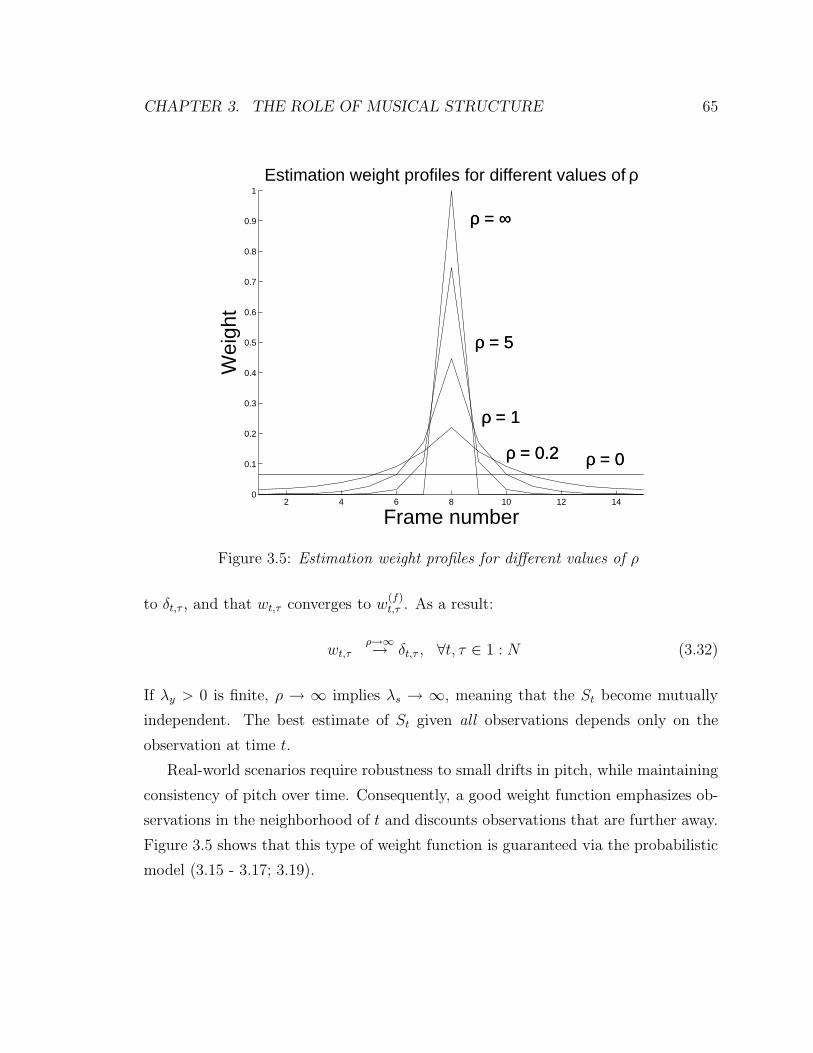
CHAPTER 3. THE ROLE OF MUSICAL STRUCTURE 65
2 4 6 8 10 12 140
0.1
0.2
0.3
0.4
0.5
0.6
0.7
0.8
0.9
1
Frame number
Wei
ght
Estimation weight profiles for different values of ρ
2 4 6 8 10 12 140
0.1
0.2
0.3
0.4
0.5
0.6
0.7
0.8
0.9
1
Frame number
Wei
ght
Estimation weight profiles for different values of ρ
ρ = ∞
ρ = 1
ρ = 0 ρ = 0.2
ρ = 5
ρ = ∞
ρ = 1
ρ = 0 ρ = 0.2
ρ = 5
Figure 3.5: Estimation weight profiles for different values of ρ
to δt,τ , and that wt,τ converges to w(f)t,τ . As a result:
wt,τρ→∞→ δt,τ , ∀t, τ ∈ 1 : N (3.32)
If λy > 0 is finite, ρ → ∞ implies λs → ∞, meaning that the St become mutually
independent. The best estimate of St given all observations depends only on the
observation at time t.
Real-world scenarios require robustness to small drifts in pitch, while maintaining
consistency of pitch over time. Consequently, a good weight function emphasizes ob-
servations in the neighborhood of t and discounts observations that are further away.
Figure 3.5 shows that this type of weight function is guaranteed via the probabilistic
model (3.15 - 3.17; 3.19).

CHAPTER 3. THE ROLE OF MUSICAL STRUCTURE 66
3.3.3 Temporal integration and abrupt change detection
Now we consider an example where pitch is consistent, but punctuated by points
of abrupt change: the “legato” model shown in Figure 3.6. The change points are
pitchedpitched pitched pitched
onset
onset
onset
onset
Figure 3.6: “Legato” model for pitch consistency with points of abrupt change
interpreted as note onsets ; they occur at unknown times. Each pair of onsets bounds
a note event. Throughout note events, pitch information is salient and consistent;
this corresponds to legato playing. We note that the legato model may be considered
as a reduction of the nominally monophonic model introduced in Section 3.4. Adding
transient regions within note events and “null” regions, which represent gaps between
note events, extends the legato model to the nominally monophonic situation.
Given the segmentation (onset times), a heuristic may be devised in which all
observations within a note event are used to estimate the pitch trajectory for any
time along that event. The observations’ weighting would follow the profiles shown
in Figure 3.5; however, zero weight would be given to observations from other note
events. Unfortunately, this segmentation is unknown. If instead we had a good
estimate of the inherent pitch trajectory, we could monitor jumps in this trajectory
to determine onset times. However, at any fixed point in time, nothing is known a
priori about the inherent pitch. As a result, we have a classic “chicken/egg” dilemma
(Figure 3.7) characteristic of such segmentation problems [50].
To resolve this situation, we encode the unknown segmentation in a hidden binary
mode variable Mt ∈ {′O′, ′C′} which indicates whether or not frame t contains an
onset. If Mt = ′O′ (onset), an onset occurs in frame t, meaning that frames t−1
and t belong to different note events. In this case we do not expect St and St−1 to

CHAPTER 3. THE ROLE OF MUSICAL STRUCTURE 67
Figure 3.7: Canonical chicken-egg situation for segmentation applications
be related. Otherwise, Mt = ′C′ (continuation), indicating that frames t − 1 and t
belong to the same note event. In this case St ≈ St−1. The directed acyclic graph of
Figure 3.8 displays the complete factorization of the joint P (M1:N , S1:N , Y1:N):
P (M1:N , S1:N , Y1:N) = P (M1)P (S1|M1)P (Y1|S1)
×N∏
t=2
P (Mt|Mt−1)P (St|St−1, Mt)P (Yt|St) (3.33)
Here P (Mt+1|Mt) follows the stochastic grammar and state transition diagram
displayed in Figure 3.9. Here the main restriction is that onsets cannot occur in
adjacent frames. The ′C′ → ′O′ transition probability p, 0 < p � 1 models the

CHAPTER 3. THE ROLE OF MUSICAL STRUCTURE 68
St-1 St St+1... ...
Yt-1 Yt Yt+1
Mt-1 Mt Mt+1
Figure 3.8: Factorization of joint distribution for legato model
O
C
p
1-p
GRAMMAR
CC C, OO(legato model)
ASSUMPTIONS:-No onsets in adjacent frames-New note events are infrequent
Figure 3.9: Stochastic grammar for mode variables, legato model
expectation that onsets are sparse6. P (Mt+1|Mt) obtains in closed form:
P (Mt+1|Mt) =
0, Mt = ′O′, Mt+1 = ′O′
1, Mt = ′O′, Mt+1 = ′C′
p, Mt = ′C′, Mt+1 = ′O′
1 − p, Mt = ′C′, Mt+1 = ′C′
(3.34)
Consistency of pitch is governed by P (St+1|St, Mt+1). If Mt+1 = ′C′, St+1 depends
6The actual value of p controls the mean note event length in the legato case. The latter isapproximately (slightly greater than) 1/p frames.

CHAPTER 3. THE ROLE OF MUSICAL STRUCTURE 69
on St in the manner of (3.17), encoding the consistency hypothesis St+1 ≈ St; oth-
erwise, if Mt+1 = ′O′, St+1 is statistically independent of St. Furthermore, the fact
that V ar(St+1|Mt+1 = ′C′) = ε−1 indicates that there lacks additional information
concerning St+1, which parallels the situation in (3.18). Hence, P (St+1|St, Mt+1) is
modeled as follows:
P (St+1|St, Mt+1 = ′C′) ∼ N (St, λs)
P (St+1|St, Mt+1 = ′O′) ∼ N(
0, ε−1)
(3.35)
The prior dependences are specified as noninformative: P (M1) uniform; P (S1|M1)
via (3.16). Finally, the observation dependence, P (Yt|St), is specified via (3.15).
The joint segmentation and pitch tracking amounts to estimating all values of the
hidden variables M1:N and S1:N , given observations Y1:N . We aim to preserve the
integrity of the entire mode sequence, M1:N , by minimizing the probability that any
such error in this sequence may occur:
M∗1:N = argmin
M1:N
P (M1:N 6= M1:N ) (3.36)
Once again, following (3.12), the optimal sequence satisfying (3.36) maximizes the
joint posterior:
M∗1:N = argmax
M1:N
P (M1:N |Y1:N) (3.37)
We note that the objective (3.36) comprises an “all or nothing” approach, penal-
izing estimates which differ from the true sequence M1:N in only one frame the same
as estimates which have nothing to do with M1:N . Furthermore, for sufficiently long
sequences and under sufficiently noisy conditions, P (M∗1:N 6= M1:N ) may approach
unity. As such, it may be preferable to minimize the expected number of frame er-
rors, following the criterion used for S1:N (3.20) in the previous section. However,
a common source of error is when the true onset sample location lies infinitesimally

CHAPTER 3. THE ROLE OF MUSICAL STRUCTURE 70
close to a frame boundary, though just preceding it; here, considerable ambiguity ex-
ists concerning whether to assign the onset to the frame in which it actually occured,
or to the subsequent frame, for which the change in the spectral content regarding
the previous frame is most salient. If M1:N declares onsets in both frames, this incurs
at most one frame error; if a single onset is declared in the wrong frame, two frame
errors result. But detecting onsets in adjacent frames is disastrous for the segmen-
tation objective, especially if the results are to be used in transcription, because this
detection introduces an extra note event. By contrast, shifting the onset location by
one frame is far less objectionable. A more striking consideration is that the joint
posterior P (M1:N |Y1:N) vanishes over sequences containing onsets in adjacent frames
because P (Mt+1|Mt) assigns these instances zero probability (3.34). Any particular
decision M∗1:N exhibiting adjacent onsets will be invalid with respect to the gener-
ative model, thus the global maximum a posteriori criterion, (3.36) guarantees the
validity of all detected mode sequences. As such, (3.37) is validated as the proper
segmentation criterion.
Regarding the estimated pitch trajectory, S∗1:N , the objective remains to minimize
the expected number of frame errors, following (3.20). However, we require addi-
tionally that S∗1:N synchronize with M∗
1:N . We cannot tolerate, for instance, a sudden
jump in S∗t+1 from S∗
t if frames t and t+1 belong to the same note event. The solution
is to choose S∗1:N minimizing expected frame error rate given M∗
1:N :
S∗t = argmax
St
P (St|Y1:N , M∗1:N) (3.38)
where M∗1:N follows via (3.36).
3.4 Nominally monophonic signals and segmenta-
tion objectives
Unfortunately, real-world musical audio signals contain regions for which steady-
state pitch content is not salient. Such regions include transients, which associate
with note events, and null regions, or gaps, which separate note events. Ideally null

CHAPTER 3. THE ROLE OF MUSICAL STRUCTURE 71
regions would contain nothing but silence. More realistically, these regions consist
of recording noise, background instrumentation, reverberation tails from past events,
and so forth.
To this end, we extend the “legato model” introduced in Section 3.3.3 to incorpo-
rate transient and null regions. The result we denote as the nominally monophonic
model, represented by the cyclic succession (transient → pitched → null) depicted in
Figure 3.10. Here each note event comprises a transient region followed by a pitched,
transient
null
transient
null
note event note event
pitched pitched
{{
onset
onset
Figure 3.10: Region characterization for nominally monophonic signals
steady-state region. Null regions separate note events. The lengths of transient and
null regions may be zero, to encode a certain flexibility towards cases where these
regions may be absent: if both transient and null lengths are zero, the legato model
results. A new note event is instantiated upon crossing of the transient boundary :
either null → transient, pitched → transient, or null → pitched transitions trigger
onsets.
We note that the nominally monophonic model fails to allow multiple pitched
and transient regions within a single note event. This becomes problematic, for
instance, in overblown flute recordings, where multiple pitched regions may occur due
to the different oscillatory regimes, and where multiple transient regions may occur
due to chaotic behavior [99]. However, the lack of an explicit model for multiple
transient/pitched regions does not cause problems in practice. First, multiple-region
instances rarely occur when dealing with single acoustic sources. Second, when these

CHAPTER 3. THE ROLE OF MUSICAL STRUCTURE 72
instances do occur, the resultant segmentation using the nominally monophonic model
retains all information concerning the locations of abrupt-change events and transient
region boundaries, the only difference being that this model declares a new note
event upon the crossing of each transient boundary within the actual event. This
information may be aggregated in postprocessing, to form the actual note events (see
Figure 3.11):
transient transient
pitched
onset
pitched pitched
transient
onset
pitchedonset
onset
note event (aggregate)true onset
null
Figure 3.11: Aggregation of note events
While the nominally monophonic model represents signals which may arise from
a monophonic “score”, the intent is to be robust to various types of polyphony; e.g.,
note overlaps due to legato playing, reverberation, or background instrumentation.
These instances occur in virtually all real-world recordings regardless of whether or not
the performance originates from a monophonic score. Such robustness considerations,
given limited computational resources, suggest the use of framewise short-time Fourier
transform (STFT) peaks as a feature set. This stands in opposition to time domain
approaches which do not attempt feature reduction, such as the methods summarized
in Chapter 1 [20, 51, 18], among possibly others. The latter methods deliver a global,
sample-accurate segmentation, but at considerable computational expense. Even in

CHAPTER 3. THE ROLE OF MUSICAL STRUCTURE 73
some offline applications such as interactive audio editing (Section 3.10.4), a sample-
accurate response may be desired.
To summarize, we obtain a robust segmentation and melody transcription for
nominally monophonic signals, defined in the sense of the transient → pitched →null cyclic succession (Figure 3.10). The segmentation operates on a quite limited yet
psychoacoustically relevant feature set (framewise sequences of STFT peaks). The
result amounts to a transcription, but is more general: not only do we detect all note
onsets, values, and durations, we provide a sub-segmentation of each event indicating
the locations of transient regions as well as steady-state regions containing pitch con-
tent. While this method fails to provide a sample accurate segmentation, it facilitates
the latter in postprocessing, by isolating region boundaries to frame neighborhoods
and identifying possible pitch content before and after the true boundary sample lo-
cation. (Given the fact that a single abrupt-change event occurs, as well as signal
models before and after change, a simple offline likelihood maximization may be used
to estimate the changepoint location; see [61], chapter 11 for further details.)
3.5 Probabilistic model
3.5.1 Variable definitions
To encode the cyclic succession (Figure 3.10) as well as label onsets at the frame
level, we introduce the mode variable Mt for frames t ∈ 1:N . Mt takes on any of the
following values:
• ′OT′ – the beginning frame of a transient region, of which there can be at most
one per note event.
• ′OP′ – the beginning frame of a note event in which the first frame already
contains salient pitch content, of which there can be at most one per note
event.
• ′CT′ – the continuation of a transient region in the event the region occupies
more than one frame; must follow a previous ′CT′ or ′OT′.

CHAPTER 3. THE ROLE OF MUSICAL STRUCTURE 74
• ′CP′ – the continuation of a pitched region; must follow an ′OP′ or ′CP′.
• ′N′ – a null frame which occurs anytime after the last frame of a note event. A
null frame is followed by another null frame, or an onset (′OT′ or ′OP′).
Table 3.1 defines special groupings of modes with common characteristics. For
Symbol Definition DescriptionP {′OP′, ′CP′} Pitched modesQ {′OT′, ′CT′, ′N′} Non-pitched modesT {′OT′, ′CT′} Transient modesO {′OT′, ′OP′} Onset modesC {′CT′, ′CP′} Continuation modes
Table 3.1: Definitions of mode groupings
instance, we represent an onset by Mt ∈ O, regardless of whether this onset occurs
in a transient or pitched frame. Additionally, it becomes convenient to define M as
the set of all modes:
M ∆= P ∪Q= O ∪ C ∪ {′N′} (3.39)
We introduce the state variable, St, to represent inherent signal characteristics
known to be consistent during steady-state portions of note events (and changing
abruptly across event boundaries) as these characteristics are primarily informative
for the segmentation. In the legato example of Section 3.3.3, St represents the inherent
pitch of the tth frame. In real-world acoustic signals, amplitude, as well as pitch,
is expected to be consistent in pitched regions. Depending on the instrument, the
amplitude may exhibit a downward bias over time (e.g., percussive instruments such as
piano and marimba), or it may exhibit equal tendencies to become softer or louder at
any point in time (wind, brass, bowed string). Hence, for the nominally monophonic
model, we encode both pitch and amplitude characteristics in St.
The pitch encoding is split among two quantities: an integer note value, plus a
fractional tuning offset. There are two advantages: first, it becomes convenient for

CHAPTER 3. THE ROLE OF MUSICAL STRUCTURE 75
the transcription task to marginalize out all but the note value, as the latter is usually
what is notated in the score. Handling note values separately also facilitates the incor-
poration of melodic expectations, as Section 3.10.1 details. Moreover, characterizing
the tuning offset as the main source of pitch drift allows the exploitation of structural
tendencies which are difficult to model otherwise. Several factors contribute to pitch
drift: first, global factors, such as the mistuning of an instrument or the playback of
the recording at a different speed. These global factors are likely to exhibit a high
degree of consistency throughout the entire recording, and they are largely indepen-
dent of the audio source and hence the region boundaries as indicated by Mt. Second,
local drifts may occur which are inherent to the acoustic source, hence responding
to note event boundaries. Examples include the pitch bend in the attack portions of
tuned percussion sources (e.g., timpani), or expressive variations such as portamento
and vibrato, found in vocals, bowed strings, and other acoustic sources.
Individual state components of note value, tuning, and amplitude are encoded as
follows:
• Nt ∈ SN = {Nmin, Nmin + 1, . . . , Nmax}, where each element of SN is an integer
representing the MIDI note value (e.g., the note C4 corresponds to Nt = 60).
• Tt ∈ ST , where ST is a uniformly spaced set of tuning values in [−0.5, 0.5), with
the minimum value equal to −0.5.
• At ∈ SA, where SA is an exponentially spaced set of reference amplitude values
active when Mt ∈ P.
• AQt ∈ SAQ, where SAQ is an exponentially spaced set of reference amplitudes
active when Mt ∈ Q.
St denotes the collection of valid possibilities for these components:
St ∈ S = SN ⊗ ST ⊗ (SA ∪ SAQ) . (3.40)
which is to say, either St = {Nt, Tt, At} if Mt ∈ P or St = {Nt, Tt, AQt }, if Mt ∈ Q.

CHAPTER 3. THE ROLE OF MUSICAL STRUCTURE 76
The STFT peak observations are represented by Yt, which consists of parallel lists
of peak frequencies and amplitudes. We represent Yt = {F, A}, where:
F∆= {F (1), F (2), . . . , F (No)}
A∆= {A(1), A(2), . . . , A(No)} (3.41)
where F (k) denotes the frequency of the kth lowest-frequency STFT peak, A(k) the
corresponding amplitude, and No the number of observed peaks. Peaks are chosen
from overlapping, Hamming windowed, zeropadded frames following the quadratic
interpolation methods described in [110, 1]; see Section 4.2.1 for further details.
The joint distribution over all variables of interest, P (M1:N , S1:N , Y1:N), factors
over the directed acyclic graph of Figure 3.12; i.e.:
P (M1:N , S1:N , Y1:N) = P (M1)P (S1|M1)P (Y1|S1)
×N∏
t=2
P (Mt|Mt−1)P (St|St−1, Mt−1, Mt)P (Yt|St) (3.42)
Mt-1 Mt
StSt-1
Yt-1 Yt
Mt+1
St+1
Yt+1
Figure 3.12: Directed acyclic graph for nominally monophonic signal model

CHAPTER 3. THE ROLE OF MUSICAL STRUCTURE 77
The essential difference between the factorization (3.42) and that of the legato
model (3.33) is the additional dependence on Mt−1 in P (St|St−1, Mt−1, Mt). The
necessity of this dependence is illustrated by the following example: if Mt = ′CP′,
either Mt−1 ∈ T or Mt−1 ∈ P. In this example t−1 and t belong to the same pitched
region of a note event; hence, we expect consistency of the corresponding pitch values:
St ≈ St−1. If Mt−1 ∈ T ⊂ Q, frame t− 1 belongs to a transient region, while frame t
belongs to a pitched region; in this case we do not expect the consistency St ≈ St−1 to
hold. We note that only the onset frame is explicitly encoded by Mt; in general, one
must examine the pair {Mt−1, Mt} to determine whether frame t crosses a particular
region boundary.
3.5.2 Inference and estimation goals
Again, recalling the legato model (Section 3.3.3), we pursue identical objectives in
terms of the segmentation. The optimal mode sequence is nothing but the global
maximum a posteriori trajectory, obtained following (3.36):
M∗1:N = argmax
M1:N
P (M1:N |Y1:N) (3.43)
We recall that M∗1:N chosen via (3.43) preserves the integrity of the entire mode
sequence, because it minimizes the probability that M∗1:N differs anywhere from the
true M1:N , regardless of how many frames make up the difference.
Individual state components, i.e., N1:N , T1:N , and (A1:N or AQ1:N) are chosen to
minimize the expected number of frame errors given M∗1:N . That is, if Zt represents
a particular state component for the tth frame, we choose:
Z∗t = argmax
Zt
P (Zt|Y1:N , M∗1:N) (3.44)
The primary inference and estimation goals consist of the computation of M∗1:N and
Z∗1:N . Secondary goals include estimating free parameters in the distributional specifi-
cation, in particular those concerning the transition dependence P (St+1, Mt+1|St, Mt),
and postprocessing for purposes of transcription, meaning the transcription of desired

CHAPTER 3. THE ROLE OF MUSICAL STRUCTURE 78
note event and transient region boundaries from M∗1:N and the assignment of pitch
information to each note via N∗1:N . Figure 3.13 summarizes the overall transcription
process.
PREPROCESSING(STFT, peak picking)
ESTIMATION OFDISTRIBUTIONAL(SIGNAL MODEL)
PARAMETERS
PRIMARYINFERENCE
P(St+1,Mt+1|St,Mt)M*1:N N*1:N T*1:N, A*1:N,A(*Q)1:N
Y1:N (framewise STFT peaks)
POSTPROCESSING
Input signal
Onsets, durations, note values, transient regions
(peaks) (notes) (tunings, amps,nullamps)
Figure 3.13: Block diagram of overall transcription process
The distributional specification is discussed below, in Section 3.6. Primary infer-
ence and parameter estimation methodologies are described in Section 3.8. However,
discussion of preprocessing stages (STFT; peak picking) is deferred to Section 4.2.1
because certain details regarding these stages relate to the modeling of peak frequency
and amplitude distributions, which is the central theme of that chapter.

CHAPTER 3. THE ROLE OF MUSICAL STRUCTURE 79
3.6 Distributional specifications
For the model in Figure 3.12, we must specify the priors P (M1), and P (S1|M1),
the transition dependence across frames: P (St+1, Mt+1|St, Mt), and the observation
likelihood P (Yt|St).
3.6.1 Prior
The role of the prior is to encode information about the first frame of the recording. If
it is known, for instance, that the recording begins with a note onset, we concentrate
P (M1) on O, the set of onset possibilities. In the most general case, however, such
knowledge is absent. Hence, we specify P (M1) as uniform and P (S1|M1) as factoring
independently among the components of S0:
P (S0|M0 ∈ P) = P (T0) P (N0) P (A0)
P (S0|M0 ∈ Q) = P (T0) P (N0) P (AQ0 ) (3.45)
where P (T0), P (N0), P (A0), and P (AQ0 ) are uniform.
3.6.2 Transition dependence
The transition dependence factors accordingly:
P (St+1, Mt+1|St, Mt) = P (Mt+1|Mt) P (St+1|Mt,Mt+1, St) (3.46)
It remains to specify mode and state dependences; respectively: P (Mt+1|Mt),
P (St+1|St, Mt, Mt+1).

CHAPTER 3. THE ROLE OF MUSICAL STRUCTURE 80
The mode transition dependence, P (Mt+1|Mt), is based around the following stan-
dard note evolution grammar encoding the cyclic succession depicted in Figure 3.10.
′OT′ → ′CT′, ′CP′
′OP′ → ′CP′, ′N′
′CT′ → ′CT′, ′CP′
′CP′ → ′CP′, ′N′, ′OT′, ′OP′
′N′ → ′OT′, ′OP′
(3.47)
The rationale behind this grammar is as follows. A primary governing princple
is that onsets, as they indicate the beginnings of note events, may not occur in
adjacent frames. In other words, an onset mode must be followed immediately by a
continuation or null mode:
P (Mt+1 ∈ C ∪N |Mt ∈ O) = 1 (3.48)
The latter ensures a well defined segmentation, especially when attack transients
occupy more than one frame. Additionally, each note event must have at least one
frame containing pitch content. The transition behavior adheres otherwise to the
cyclic succession (transient → pitched → null). where region lengths are modeled as
continuous valued random variables. Transient and null region lengths can be zero
whereas the pitched region length must be at least one frame. Since more than one
region may exist within a given frame, by convention we assign the mode Mt to be
the label of the rightmost region contained within that frame: see Figure 3.14.
The Markov transition diagram, displayed in Figure 3.15, encodes the standard
note evolution grammar, with additional tolerances for spurious incidents (e.g., an
attack transient followed immediately by silence). The latter may arise, for instance,
from the sudden “splicing” of recordings in the middle of note events. Solid lines
in Figure 3.15 represent transitions due to the standard note evolution grammar
while dotted lines represent transitions arising from spurious behaviors. The latter
transitions are assigned a small, fixed probability (on the order of 1 · 10−3).

CHAPTER 3. THE ROLE OF MUSICAL STRUCTURE 81
frame 1 frame 2 frame 3
pitchednull
transient
Figure 3.14: Schema for labeling frames according to the rightmost region assignment.In this example, frame 2 is labeled ′OP′ even though the majority of this frame isoccupied by a null region, and this frame also contains a transient region
The free parameters of P (Mt+1|Mt) are the transition probabilities for the stan-
dard note evolution grammar. Define:
pk|j∆= P (Mt+1 = k|Mt = j) ∀j, k ∈ M (3.49)
Then, let for each j ∈ M, Sj ⊂ M denote the set of possibilities for k for which pk|j
represents a transition probability in the standard note evolution grammar. Define
the vector θM as the collection of free parameters of P (Mt+1|Mt):
θM∆= Vec
⋃
j∈M
⋃
k∈Sj
{
pk|j
}
(3.50)
We estimate θM via the expectation-maximization (EM) algorithm [28]. Ideally,
θM is chosen to maximize the likelihood P (Y1:N |θM); however, the latter is generally
intractable due to the marginalization over the hidden trajectories M1:N , S1:N , of
which the number of possibilities grows exponentially with N . As such, the EM
algorithm encompasses iterations θ(i)M → θ
(i+1)M for which
{
θ(i)M , i ≥ 0
}
converges to
a local maximum of this likelihood; algorithm details are supplied in Section 3.7.2,
with additional derivations in Appendix B. A favorable initialization ensures rapid
convergence to the global likelihood maximum; we denote the latter as θ∗M .

CHAPTER 3. THE ROLE OF MUSICAL STRUCTURE 82
OT CT
CPOP
N
Figure 3.15: Markov transition diagram for P (Mt+1|Mt) .
To initialize the EM algorithm, we introduce a heterogeneous Poisson process
model representing the cyclic succession of a transient region of expected length NT ,
followed by a pitched region of expected length NP , followed by a null region of
expected length NN . Individual lengths are modeled as independent, exponentially
distributed random variables. Given the “rightmost region” assignment (Figure 3.14),
one may determine any transition probability in the initial value θ(0)M , as represented
by the nonzero elements in Table 3.2. Here, each term p(k)j,k denotes the probability
that the beginning of the next frame lies in a region of type y of the mth subsequent
cycle given that the beginning of the current frame lies in a region of type j, where
j, k ∈ {T, P, N}, and where T corresponds to a transient, P corresponds to a pitched,
and N corresponds to a null region. For example, if the current frame corresponds to
a pitched region, the probability that no transition occurs in the next frame is p(0)P,P .
The probability that the boundary of the next frame lies within the pitched region
of the subsequent note is p(1)P,P . Lastly, the probability of spurious transition, denoted
as ps, is set to some small, nonzero value; for instance, ps = 0.001 for the results of

CHAPTER 3. THE ROLE OF MUSICAL STRUCTURE 83
Section 3.9
Mt+1 = ′OT′ Mt+1 = ′OP′ Mt+1 = ′CT′
Mt =′OT′ 0 0 (1−ps)p
(0)T,T
Mt =′OP′ 0 0 0
Mt =′CT′ ps ps (1−3ps)p
(0)T,T
Mt =′CP′ p
(0)P,T p
(1)P,P 0
Mt =′N′ p
(0)N,T p
(1)N,P 0
Mt+1 = ′CP′ Mt+1 = ′N′
Mt =′OT′ (1−ps)(1 − p
(1)T,T ) ps
Mt =′OP′ p
(0)P,P 1 − p
(0)P,P
Mt =′CT′ (1−3ps)p
(1)T,T ps
Mt =′CP′ p
(0)P,P p
(0)P,N
Mt =′N′ 0 p
(0)N,N
Table 3.2: Generative Poisson model for the initialization of θM .
The state transition dependence, P (St+1|Mt, Mt+1, St), governs the expected con-
sistency between St and St+1 as a function of Mt and Mt+1. For instance, recalling
the legato model of Section 3.3.3, we expect pitch content (as represented by Nt and
Tt) to be highly consistent when frames t and t + 1 belong to pitched regions within
the same note event (Mt, Mt+1 ∈ P). In general, P (St+1|Mt, Mt+1, St) depends on Mt
at least through Mt ∈ P or Mt ∈ Q, as the relation between two temporally adjacent
pitched states is fundamentally different than the relation between a pitched state
following a non-pitched state7. No further dependence on Mt is assumed.
For fixed Mt, the variation of P (St+1|Mt, Mt+1, St) with respect to Mt+1 yields the
primary consideration for the detection of note region boundaries. Given Mt ∈ P,
Mt+1 = ′CP′ indicates that frames t and t + 1 belong to the same note event; hence
Nt+1, Tt+1, and At+1 are expected to be close to Nt, Tt, and At, respectively. On the
other hand, Mt+1 = ′OP′ signifies that frame t + 1 corresponds to the onset of a new
note event. Here, At+1 is independent of At, and Nt+1 depends only on Nt through
the probabilistic relation between the values of adjacent notes.
7This fact alone accounts for the diagonal links in Figure 3.12 which do not appear in thecorresponding graph (Figure 3.6) for the legato model, because in the latter every state is pitched.

CHAPTER 3. THE ROLE OF MUSICAL STRUCTURE 84
For fixed Mt, Mt+1 ∈ P, the transition behavior factors independently over the
components of St:
P (St+1|St, Mt+1 ∈ P, Mt ∈ P) = P (Tt+1|Tt, Mt+1, Mt ∈ P)
× P (Nt+1|Nt, Mt+1 ∈ P, Mt ∈ P) P (At+1|At, Mt+1 ∈ P, Mt ∈ P) (3.51)
Similar expressions result for Mt ∈ Q and Mt+1 ∈ Q, except in these cases At+1
is replaced by AQt+1, and At is replaced by AQ
t . We observe that the factoriza-
tion (3.51) assumes no a priori interdependence between state components when
Mt and Mt+1 are in evidence. In practice, such interdependence exists: for instance,
{Tt = 0.49, Nt = 60} and {Tt = 0.5, Nt = 61} refer to the same pitch hypothesis. The
latter ambiguity occurs upon portamento/legato transitions between notes as evi-
denced, for instance, in the violin recording analyzed in Section 3.9.1. Despite these
difficulties, the system correctly detects the onset of the second note in the transition,
and identifies the portamento pitch contour.
We discuss now the individual distributions on the r.h.s. of (3.51), considering
note, tuning, and amplitude, in that order. To begin, if Mt+1 = ′CP′, Mt ∈ Pwith probability one; hence, frames t and t + 1 belong to the same note event, and
Nt+1 ≈ Nt. In these cases, we choose the conditional distribution of Nt+1 given Nt
to concentrate about Nt. To express this concentration, we define the double-sided
exponential distribution:
E2 (X1, α+, α−|X0) =
c, X1 = X0
cαK(X1)−K(X0)+ , X1 > X0
cαK(X0)−K(X1)− , X0 > X1
(3.52)
where c is chosen such that the distribution sums to unity, and K(X) = k means that
X is the kth smallest element in the finite set of values for X. For Nt+1 given Nt, the
dependence is symmetric:
P (Nt+1|Nt, Mt+1 = ′CP′, Mt ∈ P) ∼ E2 (Nt+1|Nt, αN , αN) (3.53)

CHAPTER 3. THE ROLE OF MUSICAL STRUCTURE 85
Ideally αN = 0, but we must allow some small deviation for robustness to the
case where the tuning offset approaches ±0.5, as here some ambiguity may result as
to the note value. Now, if Mt+1 ∈ Q, no information about the note is reflected in
the observations. Here we adopt the convention that Nt+1 refers to the value of the
most recent note event; upon transition to a new event, we will have memorized the
value of the previous event and can thus apply knowledge from melodic expectations
insofar as note-to-note dependences are concerned8. Hence
P (Nt+1|Nt, Mt+1 ∈ Q, Mt ∈ M) ∼ E2 (Nt+1|Nt, αN−, αN+) (3.54)
where αN+ = αN−∆= αN . Finally, we let Pnote trans(N1|N0) be the dependence where
N0 and N1 are the values of adjacent note events; if such information is absent, the
dependence is uniform over N1, independent of N0. If Mt+1 = ′OP′, the frame t + 1
is the first frame where the value of the new note event can be observed. Since Nt
memorizes the value of the previous note, the conditional distribution of Nt+1 must
follow Pnote trans(N1|N0):
P (Nt+1|Nt, Mt+1 = ′OP′, Mt ∈ M) ∼ Pnote trans (N1|N0) (3.55)
The remaining cases involve certain (Mt, Mt+1) combinations which occur with
zero probability due to the mode transition dependence (Table 3.2). These distribu-
tions do not affect the inference outcome, so we specify them to minimize computa-
tional effort (see Table 3.3).
The conditional distribution of the tuning reflects the assumption that tuning is
8Of course, the implied first-order Markov characterization of the prior melodic structure becomesseverely inadequate when considering the structural forms implied by most musics, specifically West-ern tonal music. In the latter case, more sophisticated Markov models may be developed, such asthe model of Leistikow [71], which effectively augments Nt with past notes and intervals, as wellas higher-level contextual attributes such as key, harmony, meter, harmonic rhythm, and beat posi-tion. Leistikow’s model translates melodic expectations derived from the music cognition researchof Narmour [85], Krumhansl [64], Schellenberg [101], Lerdahl [73] Larson and McAdams [69], andothers into variable first-order Markov dependences of the form Pnote trans(N1|N0), where N0, N1
are the augmented states corresponding to successive note events; see Section 3.10.1 for furtherdetails. Whereas the simple note-to-note model is not very useful in practice, the key innovation inthe memorization of Nt in non-pitched states is to demonstrate how contextual predictions on thelevel of syntax (i.e., melodic expectations) may inform detection capabilities at the signal level.

CHAPTER 3. THE ROLE OF MUSICAL STRUCTURE 86
expected to be constant, or vary only slightly throughout the recording, indepen-
dently of onsets, offsets and note events. Of course, this is not entirely true, as some
instruments exhibit a dynamic pitch envelope. Hence
P (Tt+1|Tt, Mt+1 ∈ M, Mt ∈ M) ∼ E2 (Tt+1|Tt, αT+, αT−) (3.56)
where αT+ = αT−∆= αT indicates symmetry of the expected tuning variation. If it is
known that the pitch will decay, such as in tuned percussion sources, we may adjust
αT+ < αT− to reflect this possibility.
Finally, we consider the conditional distribution of both pitched and null ampli-
tudes. The case (Mt+1 = ′CP′, Mt ∈ P) implies that At and At+1 belong to the same
note event, At+1 concentrating about At as follows:
P (At+1|At, Mt+1 = ′CP′, Mt ∈ P) ∼ E2 (At+1|At, αA+, αA−) (3.57)
where αA+ ≤ αA−. Setting αA+ < αA− indicates a decaying amplitude evolu-
tion throughout the note duration, best adapted to percussive tones like piano and
marimba. On the other hand, setting αA+ = αA− may be more appropriate for violin,
voice, and other sustained tones, or instruments with lengthy attack regions. In all
other cases, At+1 is independent of At (or AQt ). Where Mt+1 = ′OP′, At+1 corresponds
to the pitch amplitude of the onset of a note event. In these cases, At+1 resamples
from a distribution favoring higher amplitudes:
P (At+1|At, Mt+1 = ′OP′, Mt ∈ P) ∼ E1(At+1, βA,′OP′)
P (At+1|AQt , Mt+1 = ′OP′, Mt ∈ Q) ∼ E1(At+1, βA,′OP′) (3.58)
where, using the notation of (3.52),
E1(X, β) = cβK(X) (3.59)
The constant c is chosen such that for fixed β, E1(X, β) sums to unity over
values of X. Setting βA,OP > 1 means that the pitched onset amplitude concentrates

CHAPTER 3. THE ROLE OF MUSICAL STRUCTURE 87
about higher amplitudes. Where Mt+1 ∈ ′OT′ or Mt+1 ∈ ′CT′ (i.e., Mt+1 ∈ T ), the
distribution is similar, but it concerns AQt+1 instead of At+1:
P (AQt+1|At, Mt+1 ∈ T , Mt ∈ P) ∼ E1(AQ
t+1, βA,T )
P (AQt+1|AQ
t , Mt+1 ∈ T , Mt ∈ Q) ∼ E1(AQt+1, βA,T ) (3.60)
where βA,T > 1. Where Mt+1 = ′N′, the distribution of AQt+1 follows either line of
(3.60), depending on Mt ∈ P or Q, but with βA,′N ′ < 1 in place of βA,T , since the
null mode favors lower amplitudes. Table 3.3 summarizes the aforementioned state
transition behavior, filling in ”don’t-care” possibilities.
Mt+1 Mt ∈ QP (Nt+1|Nt) ∼ E2 (Nt+1|Nt, αN , αN )
′OT′ P (Tt+1|Tt) ∼ E2 (Tt+1|Tt, αT , αT )
P (AQt+1|A
Qt ) ∼ E1(AQ
t+1, βA,T )
P (Nt+1|Nt) ∼ Pnote trans (Nt+1|Nt)′OP′ P (Tt+1|Tt) ∼ E2 (Tt+1|Tt, αT , αT )
P (At+1|AQt ) ∼ E1
`
At+1, βA,′OP′
´
P (Nt+1|Nt) ∼ E2 (Nt+1|Nt, αN , αN )′CT′ P (Tt+1|Tt) ∼ E2 (Tt+1|Tt, αT , αT )
P (AQt+1|A
Qt ) ∼ E1(AQ
t+1, βA,T )
P (Nt+1|Nt) ∼ Pnote trans (Nt+1|Nt)′CP′ P (Tt+1|Tt) ∼ E2 (Tt+1|Tt, αT , αT )
P (At+1|AQt ) ∼ E1(At+1, βA,′OP′)
P (Nt+1|Nt) ∼ E2 (Nt+1|Nt, αN , αN )′N′ P (Tt+1|Tt) ∼ E2 (Tt+1|Tt, αT , αT )
P (AQt+1|A
Qt ) ∼ E1(AQ
t+1, βA,′N′)
Mt+1 Mt ∈ PP (Nt+1|Nt) ∼ E2 (Nt+1|Nt, αN , αN )
′OT′ P (Tt+1|Tt) ∼ E2 (Tt+1|Tt, αT , αT )
P (AQt+1|At) ∼ E1(AQ
t+1, βA,T )
P (Nt+1|Nt) ∼ Pnote trans (Nt+1|Nt)′OP′ P (Tt+1|Tt) ∼ E2 (Tt+1|Tt, αT , αT )
P (At+1|At) ∼ E1`
At+1, βA,′OP′
´
P (Nt+1|Nt) ∼ E2 (Nt+1|Nt, αN , αN )′CT′ P (Tt+1|Tt) ∼ E2 (Tt+1|Tt, αT , αT )
P (AQt+1|At) ∼ E1(AQ
t+1, βA,T )
P (Nt+1|Nt) ∼ E2 (Nt+1|Nt, αN , αN )′CP′ P (Tt+1|Tt) ∼ E2 (Tt+1|Tt, αT , αT )
P (At+1|At) ∼ E2 (At+1|At, αA+, αA−)P (Nt+1|Nt) ∼ E2 (Nt+1|Nt, αN , αN )
′N′ P (Tt+1|Tt) ∼ E2 (Tt+1|Tt, αT , αT )
P (AQt+1|At) ∼ E1(AQ
t+1, βA,′N′)
Table 3.3: State transition table for component distributions of P (St+1|St, Mt+1, Mt)

CHAPTER 3. THE ROLE OF MUSICAL STRUCTURE 88
3.6.3 Frame likelihood
We wish to evaluate the likelihoods for frames with pitch content: P (Yt|Nt, Tt, At, Mt ∈P), and for frames without: P (Yt|AQ
t , Mt ∈ Q). For frames with pitch content,
P (Yt|Nt, Tt, At, Mt ∈ P) is computed by a modification of the method developed
in Chapter 4, to which we henceforth refer as the canonical evaluation. The latter
evaluates P (Yt|f0,t, A0,t) where f0,t is the radian fundamental frequency and A0,t the
reference amplitude for the tth frame, and Yt consists of the joint collection of peak
frequencies and amplitudes; i.e., Yt = {F, A}, where
F∆= {F (1), F (2), . . . , F (No)}
A∆= {A(1), A(2), . . . , A(No)} (3.61)
Here F (k) denotes the frequency of the kth lowest-frequency STFT peak and A(k)
the corresponding amplitude. We henceforth denote the canonical evaluation as
Pcan(Yt|f0,t, A0,t) to distinguish it from the subsequent modification.
The canonical evaluation proves robust to real-world phenomena such as inhar-
monicity, undetected peaks, and spurious peaks due to noise and other interfer-
ence phenomena, as indicated by the results shown in Section 4.4; see Further-
more, straightforward extensions exist for the polyphonic case; as implemented in
the Bayesian chord recognizer of Leistikow et al. [72]. However, care must be taken
in the association of the hypotheses (f0,t, A0,t) with those of the state (Nt, Tt and
At). While f0,t is uniquely determined by Nt and Tt, the relation between the ref-
erence amplitude, A0,t, and At becomes more involved. In the canonical evaluation,
the reference amplitude is estimated as the maximum amplitude over all peaks in
the frame, denoted as Amax,t. The latter yields favorable psychoacoustic properties
in the context of many real-world signals which are assumed to be monophonic, but
are actually polyphonic. For instance, consider a recording of the introductory mo-
tive of Bach’s Invention 2 in C minor (BWV 773) by Glenn Gould. Here the pianist
hums two octaves below the piano melody. The humming can barely be heard in
most frames; nevertheless, the likelihood evaluation sometimes favors the voice’s fun-
damental rather than that of the piano, especially when these fundamentals are in

CHAPTER 3. THE ROLE OF MUSICAL STRUCTURE 89
an exact harmonic relationship. While this result may be technically correct in the
absence of explicit timbral models, it fails to represent what is heard as salient. Now,
one may argue that the perceived salience of the piano melody arises from the con-
sistency of pitch and amplitude information across long segments of frames, as the
voice tends to fade in and out over these regions. We find, nevertheless, from in-
formal listening tests, that the perceived salience of the piano tone persists even in
the absence of contextual cues; for instance, when a single frame is extracted and
repeated for any given duration. A plausible explanation is that in the absence of
other contextual cues, we focus on the loudest of multiple pitch components, hence
the choice A0,t = Amax,t.
Unfortunately, use of Pcan(Yt|f0,t, A0,t) with A0,t = Amax,t ignores the state variable
At, thus preventing the conditional distribution of At from being influenced by the
signal, except indirectly via Mt. This in turn diminishes the capacity of jumps in
the signal’s amplitude envelope to inform the segmentation, which can be a critical
issue when detecting onsets of repeated notes. Our solution is to take A0,t = At
while introducing Amax,t as an independent noisy observation9 of At, as shown in
Figure 3.16. By so doing, we blend the strategy which derives A0,t from the state
(A0,t = At) with the strategy incorporating psychoacoustic salience (A0,t = Amax,t).
The conditional distribution for the observation layer becomes
P (Yt, Amax,t|Nt, Tt, At) = P (Yt|Nt, Tt, At) P (Amax,t|At) (3.62)
Here, P (Yt|Nt, Tt, At) is modeled by the canonical evaluation with A0,t = At and
f0,t the fundamental frequency corresponding to the pitch hypothesis indicated by Nt
and Tt, and Amax,t is modeled as At plus Gaussian noise:
P (Yt|Nt, Tt, At) = Pcan (Yt|f0(Nt, Tt), A0,t = At)
P (Amax,t|At) = N(
At, σ2A
)
(3.63)
9It may seem counterintuitive to model Amax,t and Yt as conditionally independent of At since,unconditionally speaking, Amax,t is a deterministic function of Yt. However, we wish not to introducebias by assuming specific dependences between the noise on Amax,t and the amplitude/frequencynoises on other peaks of Yt.

CHAPTER 3. THE ROLE OF MUSICAL STRUCTURE 90
Nt, Tt, At
Yt Amax,t
Figure 3.16: Observation layer dependence with Amax,t
We may interpolate between the rigid cases (A0,t = Amax,t vs. A0,t = At) by
varying σ2A between 0 and ∞. Assuming At ∈ R
+, as σ2A → 0, the pitch in-
ference P (Nt, Tt|Yt, Amax,t), becomes identical to the inference P ′ (Nt, Tt|Yt) where
P ′ (Yt|Nt, Tt, At) equals the canonical evaluation, P ∗ (Yt|f0(Nt, Tt), A0,t = At), with
A0,t = Amax,t. On the other hand, as σ2A → ∞, the pitch inference P (Nt, Tt|Yt, Amax,t)
converges to P (Nt, Tt|Yt), which is the canonical evaluation using A0,t = At, Amax,t
being ignored.
To show, we first consider σ2A → ∞; here the dependence on At vanishes:
P (Amax,t|At) → P (Amax,t). As a result, Amax,t and the collection {Yt, Nt, Tt, At}become mutually independent. Then P (Nt, Tt|Yt, Amax,t) → P (Nt, Tt|Yt), as was to
be shown.
Next we consider σ2A → 0; to begin, we note that in this case, P (Amax,t|At)
becomes impulsively concentrated about At; i.e.:
P (Amax,t|At) ∼ δ (Amax,t, At) (3.64)
It suffices to show that, given (3.64), P (Nt, Tt|Yt, Amax,t) becomes identical to the
inference P ′(Nt, Tt|Yt) where
P ′(Yt|Nt, Tt, At) = Pcan (Yt|f0(Nt, Tt), A0,t = Amax,t) (3.65)

CHAPTER 3. THE ROLE OF MUSICAL STRUCTURE 91
Expanding P (Nt, Tt|Yt, Amax,t) according to Bayes’ rule yields the following:
P (Nt, Tt|Yt, Amax,t) =
∑
ν,τ
∫
Atπ (At, ν, τ, Yt, Amax,t) dAt
∫
Atπ (At, Nt, Tt, Yt, Amax,t) dAt
∀ Nt, Tt (3.66)
where
π (At,Nt,Tt,Yt,Amax,t)∆= P (At,Nt,Tt,Yt,Amax,t) (3.67)
and
P (At, Nt, Tt, Yt, Amax,t) = P (At)P (Nt, Tt|At)
× Pcan (Yt|f0(Nt, Tt), A0,t = At) δ (Amax,t, At) (3.68)
Substituting (3.68) into (3.66) results in integral expressions with impulsive terms.
These expressions, and hence (3.66), simplify to
∫
At
P (At, Nt, Tt, Yt, Amax,t) dAt = P (Nt, Tt|At = Amax,t)
× Pcan (Yt|f0(Nt, Tt), A0,t = Amax,t) (3.69)
Now, since At and {Nt, Tt} are a priori independent, (3.69) simplifies further:
∫
At
P (At, Nt, Tt, Yt, Amax,t) dAt = P (Nt, Tt)
× Pcan (Yt|f0(Nt, Tt), A0,t = Amax,t) (3.70)
It follows that the substitution of (3.70) into (3.66) obtains the same relation as
the expansion of (3.65) via Bayes’ rule, in parallel fashion to (3.66). Hence
P (Nt, Tt|Yt, Amax,t) = P ′ (Nt, Tt|Yt, Amax,t) (3.71)
as was to be shown.
In the preceding development, the space of At was assumed to be R+ which is an
uncountably infinite space. In actuality the domain of At is limited and the space

CHAPTER 3. THE ROLE OF MUSICAL STRUCTURE 92
discretized to a finite set of possibilities. Nevertheless, provided the domain’s extent
is sufficiently large, and σ2A considerably exceeds the square of the largest spacing
between At values, the results realized “in practice” become virtually identical to the
analyzed situation where At ∈ R+.
As a final note, some frames may lack pitch content altogether; these correspond to
purely transient effects (e.g., percussion), background noise, or silence. In these cases
Mt ∈ Q. Since we still wish to model a general amplitude characteristic associated
with these frames, in order to distinguish transients from silence, for instance, we
model the frame via Pcan(Yt|f0(Nt, Tt), AQt ) under the restriction that all peaks are
spurious.
3.7 Inference methodology
3.7.1 Primary inference
The primary inference goals for the joint onset detection, transient region identifica-
tion, and melody transcription, as discussed in Section 3.5.2, are the determination
of the maximum a posteriori mode sequence M∗1:N ; i.e.,
M∗1:N = argmax
M1:N
P (M1:N |Y1:N) (3.72)
and the computation of the smoothed state posterior given M∗1:N ; denoted as σ∗
1:N ;
i.e.,
σ∗(St) = P (St|M∗1:N , Y1:N), ∀t ∈ 1 : N (3.73)
If, for any t ∈ 1 : N − 1, Yt+1 is conditionally independent of Y1:t and M1:t given
Mt+1, the Viterbi algorithm [94] may be used to identify M∗1:N . Unfortunately, the
implicit marginalization of S1:N in P (M1:N |Y1:N) precludes this possibility. As the
complexity of the Viterbi approach is linear in the number of frames and quadratic

CHAPTER 3. THE ROLE OF MUSICAL STRUCTURE 93
in the number of modes, we seek an approximate Viterbi inference with similar com-
putational cost. To this end, we approximate:
P (Yt+1|M1:t+1, Yt) ≈ P (Yt+1|M∗1:t−1(Mt), Mt, Mt+1, Y1:t) (3.74)
where
M∗1:t−1(Mt) ≈ argmax
M1:t−1
P (M1:t−1|Mt, Y1:t) (3.75)
We refer to M∗1:t−1(Mt) as the (approximate) Mt-optimal mode sequence, and define
M∗a:b(Mt) as the restriction of this sequence to frames a through b, and adopt the
shorthand M∗a
∆= M∗
a:a. This approximation, similar to that used by Pavlovic et al.
[87] for the learning of switching linear models of human motion, treats the history
of the mode sequence up to time t− 1 collectively as a nuisance parameter, replacing
its value with the corresponding maximum a posteriori estimate given Mt and Y1:t.
The inference proceeds in two passes, a forward, filtering pass, followed by a
backward, smoothing pass. Table 3.4 summarizes the quantities propagated in these
passes, as well as the necessary input distributions (the conditional dependences on
the r.h.s. of the factorization (3.42)). The designation (≈) means the referenced
quantity is approximate.
Symbol Quantity Descriptionτ∗(Mt, St) P (St|M∗
1:t−1(Mt), Mt, Y1:t−1) Predicted posterior givenMt-optimal mode sequence
µ∗(Mt, St) P (St|M∗1:t−1(Mt), Mt, Y1:t) Smoothed posterior given
Mt-optimal mode sequenceJ(Mt) maxM1:t−1
P (M1:t|Y1:t) (≈) Objective at time t
M∗t−1(Mt) argmaxMt−1
maxM1:t−2P (M1:t|Y1:t) (≈) Backpointer
M∗t argmaxMt
maxM1:t−1,Mt+1:NP (M1:N |Y1:N ) (≈) MAP mode at time t
σ∗t (St) P (St|M∗
1:N , Y1:N ) Smoothed posteriorµ0(Mt, St, Mt+1) P (St+1, Yt+1|M∗
1:t−1(Mt), Mt, Mt+1, Y1:t) Intermediate
τ(Mt, St, Mt+1) P (St+1|M∗1:t−1(Mt), Mt, Mt+1, Y1:t) Intermediate
µ(Mt, St, Mt+1) P (St+1|M∗1:t−1(Mt), Mt, Mt+1, Y1:t+1) Intermediate
Σ0(Mt, Mt+1) P (Yt+1|M∗1:t−1(Mt), Mt+1, Y1:t+1) Intermediate
J0(Mt, Mt+1) maxM1:t−1P (M1:t+1|Y1:t+1) (≈) Intermediate
Table 3.4: Approximate Viterbi inference inputs and propagated quantities
The computation of M∗1:N and {σ∗(St)}N
t=1 via Table 3.4 satisfies (3.72) and (3.73),
as desired.

CHAPTER 3. THE ROLE OF MUSICAL STRUCTURE 94
To begin, the filtering pass is initialized as follows.
µ∗(S1, M1) = P (M1, S1|Y1)
=P (S1|M1)P (Y1|S1)
∑
S1P (S1|M1)P (Y1|S1)
J(M1) = P (M1|Y1)
=P (M1)
∑
S1P (S1|M1)P (Y1|S1)
∑
M1P (M1)
∑
S1P (S1|M1)P (Y1|S1)
(3.76)
Then, for t ∈ 1 : N − 1, the filtering recursions proceed:
τ (Mt, St, Mt+1) =∑
St
µ∗ (Mt, St) P (St+1|Mt, Mt+1, St)
µ0 (Mt, St, Mt+1) = P (Yt+1|St+1) τ (Mt, St, Mt+1)
Σ0 (Mt, Mt+1) =∑
St+1
µ0 (Mt, St, Mt+1)
J0 (Mt, Mt+1) = J (Mt)P (Mt+1|Mt) Σ0 (Mt, Mt+1)
µ (Mt, St, Mt+1) =µ0 (Mt, St, Mt+1)
Σ0 (Mt, Mt+1)
M∗t (Mt+1) = argmax
Mt
J0 (Mt, Mt+1)
J (Mt+1) =J0 (Mt, Mt+1)
P (Yt+1|Yt)
µ∗ (St, Mt) = µ (St+1, M∗t (Mt+1) , Mt+1)
τ ∗ (St, Mt) = τ (St+1, M∗t (Mt+1) , Mt+1) (3.77)
For t ≥ 1, µ∗(Mt, St) and M∗t (Mt+1) are stored as well as τ ∗(Mt, St) for t ≥ 2, and
J(MN). These quantities are necessary for efficient computation of the smoothing
pass. The latter is initialized as follows.
M∗N = argmax
MN
J (MN )
σ∗(SN ) = µ∗(SN , M∗N) (3.78)

CHAPTER 3. THE ROLE OF MUSICAL STRUCTURE 95
Smoothing recursions proceed as t decreases from N − 1 down to 1, as follows:
M∗t = M∗
t (M∗t+1)
σ∗(St) = µ∗(St, M∗t )∑
St+1
σ∗(St+1)P (St+1|St, M∗t , M∗
t+1)
τ ∗(St+1, M∗t+1)
(3.79)
Recursions (3.76 - 3.78) are derived in Appendix A.
Finally, we still need to compute the smoothed posteriors for the individual com-
ponents of St as required by (3.44). These are given by marginalizing out the other
components of St according to the definitions (3.40). There are two cases: M∗t ∈ P,
or M∗t ∈ Q:
P (Nt|M∗1:N , Y1:N) =
∑
Tt,At
P (St|M∗1:N , Y1:N), M∗
t ∈ P
P (Nt|M∗1:N , Y1:N) =
∑
Tt,AQt
P (St|M∗1:N , Y1:N), M∗
t ∈ Q (3.80)
P (Tt|M∗1:N , Y1:N) =
∑
Nt,At
P (St|M∗1:N , Y1:N), M∗
t ∈ P
P (Tt|M∗1:N , Y1:N) =
∑
Nt,AQt
P (St|M∗1:N , Y1:N), M∗
t ∈ Q (3.81)
P (At|M∗1:N , Y1:N) =
∑
Tt,Nt
P (St|M∗1:N , Y1:N), M∗
t ∈ P
P (AQt |M∗
1:N , Y1:N) =∑
Tt,Nt
P (St|M∗1:N , Y1:N), M∗
t ∈ Q (3.82)

CHAPTER 3. THE ROLE OF MUSICAL STRUCTURE 96
3.7.2 Estimation of free parameters in the mode transition
dependence
Recall from Section 3.6.2 that the free parameters of the mode transition dependence
P (Mt+1|Mt), may be encoded in the vector θM :
θM∆= Vec
⋃
j∈M
⋃
k∈Sj
{
pk|j
}
(3.83)
where Sj ⊂ M denotes the set of possibilities for k for which pk|j∆= P (Mt+1 = k|Mt = j)
represents a transition probability in the standard note evolution grammar (3.47).
The EM algorithm for estimating θM , introduced in Section 3.6.2, begins with
an initial guess, i.e., θ(0)M , and proceeds over iterations i, updating the estimate θ
(i)M .
Iterations repeat until convergence. Each iteration updating θ(i)M → θ
(i+1)M consists of
two steps:
• E-step: Compute as follows:
σ(2)(Mt, Mt+1) = P (Mt, Mt+1|Y1:N , θ(i)M ) (3.84)
for all t ∈ 1 : N − 1 and Mt, Mt+1 ∈ M.
• M-step: Update for each j ∈ M, k ∈ Sj :
p(i+1)k|j =
∑N−1t=1 σ(2)(Mt = j, Mt+1 = k)
∑
k∈M
∑N−1t=1 σ(2)(Mt = j, Mt+1 = k)
(3.85)
A complete derivation of the EM algorithm steps is provided in Appendix B, Section
B.1 while the computation of the pairwise smoothed posterior P (Mt, Mt+1|Y1:N , θ(i)M )
is addressed in Section B.2.

CHAPTER 3. THE ROLE OF MUSICAL STRUCTURE 97
3.8 Postprocessing
The goal of postprocessing is to take the maximum a posteriori mode sequence,
M∗1:N , (3.43) and the smoothed note posterior P (Nt|M∗
1:N , Y1:N), and produce a string
of distinct note events. These events can be stored in a MIDI file. With additional
metrical information, one may further process the note event stream to produce a
score-based representation. However, doing so properly depends on the ability to
model uncertainties in metrical structure, and to integrate such models with signal
information, which lies beyond the scope of the current work. By augmenting the
state Nt with past note values and intervals, as well as higher-level information such
as key, harmony, meter, harmonic rhythm, and beat position, the transition distri-
bution Pnote trans(N1|N0) may represent such uncertainties. Since this distribution is
activated upon transition into the first pitched frame of a new note event, following
(3.55), it serves thus to integrate both signal-level and symbolic-level dependences.
Forthcoming work by Leistikow [71] makes explicit, among other things, the use of
the augmented Nt representation in the modeling of metrical structure (i.e., deter-
mination of bar lines) and hence the production of scores from MIDI files. The bar
line determination problem is well studied; see [3, 21, 30, 113] among others. Other
issues which aid the MIDI → score conversion, such as pitch spelling determination,
are addressed in [22, 23] and the listed references therein, among other sources.
In the present (MIDI file) output, each event consists of an onset time, note
value, and duration. Additionally, we provide a sub-segmentation into transient and
pitched regions. Since the nominally monophonic model (Figure 3.10) is restricted
to having for each note event, at most one transient region followed by a pitched
region, it suffices for the sub-segmentation to specify the duration of the transient
region. Table 3.5 summarizes the symbols defined to represent these quantities; here,
all symbols refer to the kth note event.
Now let Z be a collection of distinct integers, and let min(Z) be the minimum
integer in the collection if Z is nonempty. Define:
+
min(Z)∆=
{
∞, Z = ∅min(Z) otherwise
(3.86)

CHAPTER 3. THE ROLE OF MUSICAL STRUCTURE 98
Symbol Description
o(k) Onset frame for note event
p(k) First pitched frame in note event
d(k) Note event duration
e(k)+ One frame beyond end of note event
N∗(k) MIDI note value
Table 3.5: Transcription output quantities
The postprocessing algorithm iterates over note events k, stopping only when either
the onset frame, pitch boundary, or the advanced end point (o(k), p(k), or e(k)+ ), are
infinite. This stopping condition indicates that there is not enough signal to determine
information about the current or subsequent note events.
The onset frame for the first event is initialized as follows.
o(1) =+
min {t ≥ 1 : M∗t ∈ O} (3.87)
This search for an explicit onset automatically discards tail portions of note events
which are truncated by the beginning of the signal.
In general, the recursions used to extract note events information are as follows:
o(k) =+
min{
t ≥ e(k−1)+ : M∗
t ∈ O}
p(k) =+
min{
t ≥ o(k) : M∗t ∈ P
}
e(k)+ =
+
min{
t ≥ p(k) : M∗t /∈ C
}
(3.88)
If k = 1, the initialization (3.87) is used in place of (3.88) in case of o(k). As indicated,
e(k)+ lies one frame beyond the last frame of the note event. The duration of note k
is just the simple difference between e(k)+ and o(k), unless e
(k)+ has been truncated by
the end of the signal. In the latter case, the duration is that of the truncated part:
N − o(k) + 1.
d(k) = min(e(k)+ , N + 1) − o(k) (3.89)

CHAPTER 3. THE ROLE OF MUSICAL STRUCTURE 99
To obtain the MIDI note value, we extract:
N∗(k) = argmaxn
P (Np(1)+c = n|Y1:N) (3.90)
where
c = min(c0, e(k)+ − p(1) − 1). (3.91)
Here c is a margin variable ensuring that the maximum a posteriori pitch value
assigned to the entire event is sampled from a frame which is some distance away
from the end of the transient region. The canonical value of c, ignoring truncation
effects, is c0; c0 = 3 is used to generate the examples of Section 3.9.
We note that the the algorithm seems relatively insensitive to c0 due to consistency
of Nt during pitch regions.. Clearly, the greater the a priori consistency, the more
consistent the maximum a posteriori estimates: signal information is weighted more
uniformly during pitched regions to estimate Nt along any point in the region; as
apparent in the observation weightings for the legato model example of Figure 3.5.
Recalling (3.53), the consistency of Nt during pitched regions is captured by the
following distribution:
P (Nt+1|Nt, Mt+1 = ′CP′, Mt ∈ P) ∼ E2 (Nt+1|Nt, αN , αN) (3.92)
where the double-sided exponential, E2, is defined by (3.52). The amount of consis-
tency is governed by αN in the sense that αN ↓ 0 indicates that all note values must
be identical during the entire pitched region.
In practice, it is virtually unheard of for the maxmized note posterior to fail to be
identical during the pitched portions of note events, as even extreme vibrato effects
may be absorbed by tuning offset variations. Hence, there is no loss of generality in
setting αN = 0, implying that the actual value of c0 specified in (3.90) is immaterial,
as long as c0 > 0.

CHAPTER 3. THE ROLE OF MUSICAL STRUCTURE 100
3.9 Results
The system for joint onset detection, transient region identification, and melody tran-
scription developed in the preceding sections has been applied to a variety of piano
and violin recordings. While each recording arises from a monophonic score, in ac-
tuality they contain instances of polyphony due to reverberation, note overlaps from
legato playing, and background instrumentation. Furthermore, expressive pitch vari-
ations such as portamento and vibrato occur in the violin passages. The goal of this
section is to provide a detailed analysis of the system’s performance for one repre-
sentative example of each type: a piano recording in which the performer also sings
in the background, and a violin recording exhibiting significant reverberation, legato
playing and expressive pitch variation.
The piano recording consists of the introductory motive of Bach’s Invention II in
C minor (BWV 773), performed by Glenn Gould. The top section of Figure 3.17
displays the time domain waveform. While this recording lacks significant reverber-
ation, the legato playing style nevertheless causes many notes to overlap. A further
complication is that the performer (Gould) accompanies himself with low-amplitude
vocalizations, with fundamentals approximately two octaves below those of the pi-
ano10. Nevertheless, onsets are clearly visible and may be determined by standard
heuristic time domain approaches which monitor jumps in the amplitude envelope;
see, for instance, the algorithm of Schloss [102] used in the automatic transcription of
percussive music. The purpose of this example is mainly to show robustness to low
levels of background instrumentation.
The violin recording is an excerpt from the third movement of Bach’s solo violin
Sonata No. 1 in G minor (BWV 1001), performed by Nathan Milstein. The top
section of Figure 3.18 displays the time domain waveform. This recording is awash
in reverberation, which makes it difficult to detect onsets visually or by monitoring
the amplitude envelope. Furthermore, excessive reverberation combined with legato
playing induces significant polyphony due to overlapping notes. Expressive pitch
variations, particularly portamento, create ambiguities concerning onset locations. A
10This idiosyncrasy of Gould has been well documented; see Malone [80] for an interesting studyof counterpoint with regards to the piano material as appearing in Gould’s vocalizations.

CHAPTER 3. THE ROLE OF MUSICAL STRUCTURE 101
significant “slide” (legato/portamento transition), for instance, exists between the
third and fourth notes.
3.9.1 Primary inference
Primary inference concerns the determination of the maximum a posteriori mode se-
quence M∗1:N and the and the computation of the smoothed posteriors for note, tuning
offset, and pitched/non-pitched reference amplitude (3.80 - 3.82). Figure 3.17 displays
results for the piano example. The time domain waveform is displayed at the top of
Figure 3.17. Vertical lines designate frame boundaries. In the section labeled “On-
set”, a black rectangle is displayed for each frame t for which M∗t ∈ O. The section
labeled “Modes” displays for each M ∈ M, a black rectangle for each frame in which
M∗t = M . The remaining sections, entitled “Notes”, “Tunings”, “Amps”, and “Nul-
lAmps”, display rectangles with sizes depending on the value of the posterior for each
quantity and frame. (e.g., the “Tunings” section displays P (Tt|M∗1:N , Y1:N)). Rect-
angle sizes vary logarithmically according to posterior probability, with the smallest
visible rectangle corresponding to a probability of 0.03, and the largest, 1.0.
In this example, since visual inspection of the amplitude envelope essentially indi-
cates the proper segmentation, it is easy to check that the sequence M∗1:N and hence
the onset determination are valid. The note posteriors, P (Nt|M∗1:N , Y1:N) concentrate
almost perfectly about the correct note values during pitched portion of note events,
despite the occasional presence of the performer’s voice, and the overlapping decays
(significant overlaps are observed between the second and third notes, as well as be-
tween the third and fourth). The concentration of the note posterior extends beyond
the ends of these regions, encompassing null and transient regions until the beginning
of the pitched region for the following event. The latter observation is consistent with
the reuse of Nt during non-pitched regions to “memorize” the previous note value,
as discussed in Section 3.6.2. The tuning posterior, P (Tt|M∗1:N , Y1:N), seems remark-
ably consistent and only slightly influenced by note boundaries (the maximum of this
posterior deviates ±10 cents for the third and fifth notes). The (pitched) amplitude
posterior, P (At|M∗1:N , Y1:N), indicates decaying envelopes as expected for piano.

CHAPTER 3. THE ROLE OF MUSICAL STRUCTURE 102
10 20 30 40 50 60 70 80 90 100 110 120 130 140 150Frames
0.0501
0.0006NullAmps
55.2931
0.6911Amps
0.41
−0.50
Tunings
80
44
Notes
N CP CT OP OT
Modes
onOnset−1.0
0.0
1.0
Signal
Figure 3.17: Piano example: Introductory motive of Bach’s Invention 2 in C minor(BWV 773), performed by Glenn Gould

CHAPTER 3. THE ROLE OF MUSICAL STRUCTURE 103
Corresponding results for the violin example are displayed in Figure 3.18. Since
onsets are not directly visible by eye, checking the validity of the segmentation in the
violin example becomes a painstaking process in which one must repeatedly splice
and listen to various extracts, each time shifting the possible note boundaries. This
process may take several minutes for each second of music. Further complications
arise thanks the to shortness of the segments and the significant polyphony induced
by reverberation and legato playing. Nevertheless, it seems difficult to improve on
the resultant segmentation as indicated by M∗1:N .
Through maximizing the note posterior, P (Nt|M∗1:N , Y1:N), all notes are correctly
detected except for the initial “grace note” comprising the first three frames11. For
these frames, the detected pitch is one octave below the notated pitch. The tuning
posterior is less consistent than in the piano example, primarily due to portamento.
We see that the overt slide between the third and fourth notes manifests in the drift
of the maximized tuning posterior about the onset of the fourth note.
3.9.2 Estimation of mode transition dependence
The convergence of the EM iterations for estimating P (Mt+1|Mt) is displayed in
Figure 3.19 for the Poisson initialization and in Figure 3.20 for a uniform initialization.
The latter is provided for purposes of comparison. These figures refer to the piano
example generating the primary inference results of Figure 3.17. States labeled on the
horizontal axis correspond to Mt+1; the vertical axis, Mt. Black rectangles are used
to display the transition probabilities P (Mt+1|Mt); the size of each rectangle varies
logarithmically with the probability value according to the schema of the previous
section (Figures 3.17 and 3.18). That is, the smallest visible rectangle corresponds to
a transition probability of 0.03 while the largest corresponds to a probability of 1.0.
Recall that the Poisson initialization encodes knowledge of the “cyclic succession”
schema (Figure 3.10), where a transient region of expected length NT is followed by
a pitched region of expected length NP , followed by a null region of expected length
NN , and repeating until the end of the signal. Individual region lengths are modeled
11The note in question is not an actual grace note, but an artifact due to truncation of all butthree frames from the previous note event.

CHAPTER 3. THE ROLE OF MUSICAL STRUCTURE 104
10 20 30 40 50 60 70 80 90 100 110Frames
0.0501
0.0006NullAmps
55.2931
0.6911Amps
0.41
−0.50
Tunings
80
44
Notes
N CP CT OP OT
Modes
onOnset−1.0
0.0
1.0
Signal
Figure 3.18: Primary inference results on an excerpt from the third movement ofBach’s solo violin Sonata No. 1 in G minor (BWV 1001), performed by NathanMilstein

CHAPTER 3. THE ROLE OF MUSICAL STRUCTURE 105
OT OP CT CP N
N
CP
CT
OP
OT
(a) Init
OT OP CT CP N
N
CP
CT
OP
OT
(b) Iter. 1
OT OP CT CP N
N
CP
CT
OP
OT
(c) Iter. 2
OT OP CT CP N
N
CP
CT
OP
OT
(d) Iter. 3
OT OP CT CP N
N
CP
CT
OP
OT
(e) Iter. 4
OT OP CT CP N
N
CP
CT
OP
OT
(f) Iter. 5
Figure 3.19: EM convergence results beginning from Poisson initialization
as independent, exponentially distributed random variables. We choose mean lengths
of NT = 23 ms, NP = 580 ms, and NN = 348 ms 12. The EM convergence, however,
appears relatively insensitive to modest variations in mean lengths.
The uniform initialization attempts to remove all prior knowledge from the speci-
fication of θ(0)M , distributing transition probabilities in a conditionally uniform manner
given Sj ∈ M for each j ∈ M after accounting for spurious transitions. To represent
the latter, let Sspurj denote for each j ∈ M, the collection of k ∈ M for which the
j → k transition is spurious, meaning that it appears as a dotted line in Figure 3.15.
Then, according to (3.83), we may represent θ(0)M as follows:
θ(0)M
∆= Vec
⋃
j∈M
⋃
k∈Sj
{
p(0)k|j
}
(3.93)
12With 44100 Hz sampling rate and 1024-sample frames, these settings are achieved with NT = 1frame, NP = 25 frames, and NN = 15 frames.
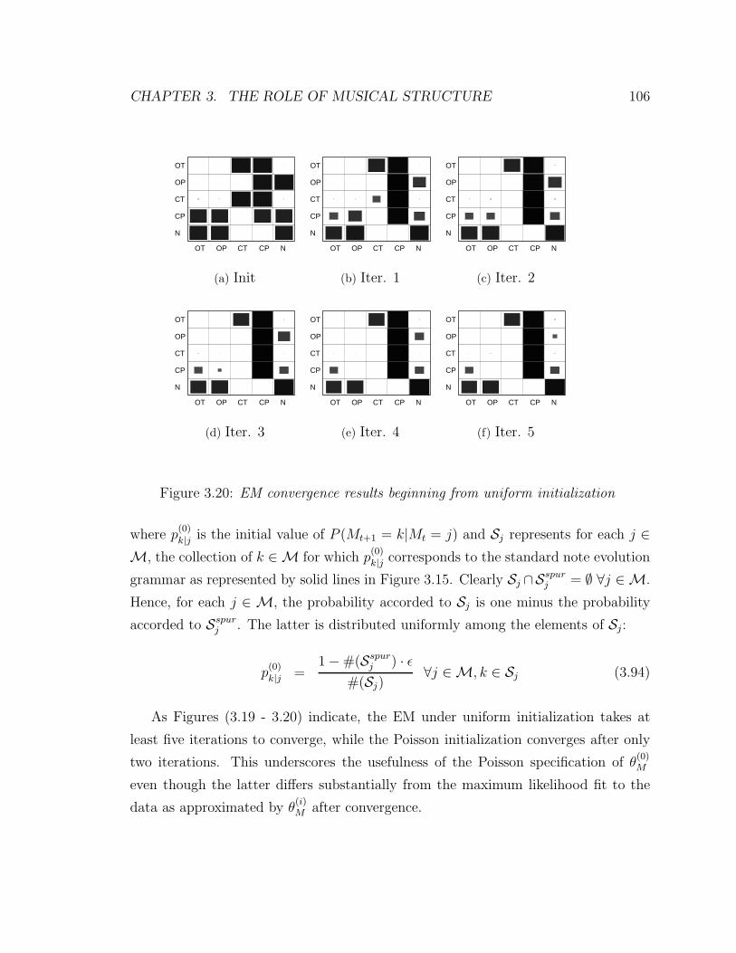
CHAPTER 3. THE ROLE OF MUSICAL STRUCTURE 106
OT OP CT CP N
N
CP
CT
OP
OT
(a) Init
OT OP CT CP N
N
CP
CT
OP
OT
(b) Iter. 1
OT OP CT CP N
N
CP
CT
OP
OT
(c) Iter. 2
OT OP CT CP N
N
CP
CT
OP
OT
(d) Iter. 3
OT OP CT CP N
N
CP
CT
OP
OT
(e) Iter. 4
OT OP CT CP N
N
CP
CT
OP
OT
(f) Iter. 5
Figure 3.20: EM convergence results beginning from uniform initialization
where p(0)k|j is the initial value of P (Mt+1 = k|Mt = j) and Sj represents for each j ∈
M, the collection of k ∈ M for which p(0)k|j corresponds to the standard note evolution
grammar as represented by solid lines in Figure 3.15. Clearly Sj ∩Sspurj = ∅ ∀j ∈ M.
Hence, for each j ∈ M, the probability accorded to Sj is one minus the probability
accorded to Sspurj . The latter is distributed uniformly among the elements of Sj:
p(0)k|j =
1 − #(Sspurj ) · ε
#(Sj)∀j ∈ M, k ∈ Sj (3.94)
As Figures (3.19 - 3.20) indicate, the EM under uniform initialization takes at
least five iterations to converge, while the Poisson initialization converges after only
two iterations. This underscores the usefulness of the Poisson specification of θ(0)M
even though the latter differs substantially from the maximum likelihood fit to the
data as approximated by θ(i)M after convergence.

CHAPTER 3. THE ROLE OF MUSICAL STRUCTURE 107
3.10 Conclusions and future work
As demonstrated in the previous section, the proposed method is able to accurately
segment and extract melodies from framewise STFT peak data obtained from nom-
inally monophonic recordings. The method not only identifies note boundaries, it
yields a sub-segmentation of each note into transient and steady-state regions. The
latter proves useful for the analysis-synthesis tasks of Chapter 2, for instance the time
and pitch scaling discussed in Section 2.2, and the transient-specific processing intro-
duced in Section 2.3. Additionally, the sub-segmentation finds application in adaptive
window switching for audio transform coding [36]. Since transient regions generally
contain broadband, rapidly time-varying spectral content, it is advantageous to use
short windows to analyze these regions, because short windows sacrifice frequency
resolution for increased time resolution. Shorter windows are used for transients and
longer windows for the steady-state parts.
The proposed method proves robust to noise, interference, expressive pitch vari-
ations resulting from portamento and vibrato, and instances of polyphony resulting
from background instrumentation, note overlaps due to legato playing, and rever-
beration. Robustness is aided by the temporal integration caused by modeling prior
structural information at the signal level as captured by the “standard note evolution”
grammar (3.47) as well as the expectation that pitch and amplitude characteristics
will be consistent throughout pitched regions of note events. As a result, all frames
within each pitched region are used to estimate signal characteristics (pitches and
amplitudes) during any point in the region.
Furthermore, the proposed method facilitates the modeling of higher-level struc-
tural attributes via melodic expectations, and the integration of such attributes
with the signal-level information. Melodic expectations are presently modeled via
Pnote trans(N1|N0), the note-to-note transition distribution introduced in Section 3.6.2.
Unfortunately, this first-order Markov dependence may not capture the majority of
expectations which arise in practice, particularly in the context of Western tonal
music [69]. Forthcoming work by Leistikow [71] considers the augmentation of the
Nt-encoding to include past notes and intervals, as well as higher-level context (e.g.,

CHAPTER 3. THE ROLE OF MUSICAL STRUCTURE 108
key, harmony, meter, harmonic rhythm, and beat position) so that these expecta-
tions may be represented using a first-order Markov dependence, which may be in-
corporated into the present method. Section 3.10.1 summarizes key features of this
approach.
In addition to melody, another important high-level structural attribute is rhythm.
Rhythm manifests in quasi-regular patterns of onset times (and other region boundary
times) about which listeners develop temporal expectations. The latter take the form
of a hazard rate influencing the distribution P (Mt+1|Mt). Temporal expectations
involving rhythmic structure may be modeled via probabilistic phase locking networks,
as introduced in Section 3.10.1.
Subsequent work should also address several limitations of the proposed method.
First, the method currently lacks the ability to encode actual instances of polyphony,
so it cannot be used to transcribe recordings generated from polyphonic scores. In Sec-
tion 3.10.3, a straightforward polyphonic extension is proposed. Second, the method’s
temporal resolution for determining segment boundaries is restricted by the frame rate
(equivalent to the STFT hop size). For instance, the results of Figures 3.17 and 3.18
use a frame rate of 512 samples at 44.1 kHz (11.6 ms), which may not suffice for
either analysis-synthesis or transform coding applications. Nevertheless, the frame-
resolution output yields significant information about the location of onsets and other
transient boundaries, as well as signal models before and after change. As discussed in
Section 3.10.4, this information may be useful in subsequent sample accurate process-
ing. In this section, we propose additional applications in interactive audio editing.
For instance, given a nominally monophonic recording with overlapping notes, one
may select all note events of a given type (such as the stable notes with respect to the
current harmony), demix them from the recording, process them individually, and
mix the processed versions in with the rest of the recording.
3.10.1 Modeling melodic expectations
Currently, one may integrate melodic expectations into the present system in the
form of a stationary, first-order Markov dependence, Pnote trans(N1|N0), where N1

CHAPTER 3. THE ROLE OF MUSICAL STRUCTURE 109
represents the current note and N0 the previous. However, this dependence proves
insufficient to model even the simplest melodic expectations which arise in most
musics, for instance Western tonal music.
Much recent work in the music cognition literature (cf. Krumhansl [64], Narmour
[85], Schellenberg [101], and Larson and McAdams [69]) addresses the fundamental
melodic expectations which arise in Western tonal music. Unfortunately, these ex-
pectations are given in rule based, instead of probabilistic, form. To be of use in the
present system, these models must admit a stationary first-order Markov probabilis-
tic representation with respect to some encoding which advances on a note-by-note
basis. In forthcoming work, Leistikow [71] solves this issue by expanding the note
representation to include additional state information which makes the Markov rep-
resentation possible. Leistikow’s representation augments the current note value with
past notes and intervals, as well as higher-level contextual attirbutes, for instance,
key, harmony, meter, harmonic rhythm, and beat position.
We may summarize Leistikow’s representation as follows. Let Xk denote the
augmented note representation, where k is the note index. The goal is to encode the
melodic expectations as described in the aforementioned music cognition work in the
form of P (X1|X0) (which by assumed stationarity equals P (Xk|Xk−1) for any k). A
common feature of the aforementioned music cognition work is that, given particular
values of Xk−1, certain values of Xk (or subsets of such values) are expected to
occur more frequently than others. This expectation does not determine P (Xk|Xk−1),
inasmuch as it constrains it; the form of such constraints are clearly convex over the
product space of simplices representing possibilities for P (Xk|Xk−1). For example,
consider the “musical force” expectations introduced by Larson and McAdams [69],
namely inertia, magnetism, and gravity.
• Inertia says that if a melody makes at least two stepwise transitions in a given
direction (up or down), the following note will be more likely to continue that
direction than reverse course.
• Magnetism involves the current key, which generates a collection of stable note
values corresponding to the tonic major triad (i.e., if the key is ′C Major′, the

CHAPTER 3. THE ROLE OF MUSICAL STRUCTURE 110
′C′, ′E′, and ′G′ notes constitute the stable notes for each octave). Magnetism
says that if the choice is between a stepwise transition towards or away from the
nearest stable note, the transition towards that note will be more likely; i.e., in
the ′C Major′ example, the transition ′F′ → ′E′ is more likely than ′F′ → ′G′.
• Similarly, gravity says that unstable notes are more likely to descend then ascend
along stepwise transitions.
Now, consider
Xk∆=
{
N(0)k , I
(1)k , I
(2)k , Kk
}
(3.95)
where N(0)k is the current (kth) note value, I
(1)k ∈ I is a type designation for the
interval leading up to N(0)k , I
(2)k is the preceding interval designation, and Kk is the
key. The set I consists of five interval types:
I = {′R′, ′SU′, ′SD′, ′LU′, ′LD′} (3.96)
where
• ′R′ means repeat ; the current and previous notes are identical
• ′SU′ means step up; the current note is one or two semitones above the previous
• ′SD′ means step down; the current note is one or two semitones below the
previous
• ′LU′ means leap up; the current note is at least three semitones above the
previous
• ′LD′ means leap down; the current note is at least three semitones below the
previous
Since many elements of the pair {Xk−1, Xk} are redundant (e.g., I(2)k = I
(1)k−1) P (Xk|Xk−1)
factors into P (Kk|Kk−1), P (N(0)k |N (0)
k−1, I(1)k−1, I
(2)k−1, Kk), and a number of degenerate

CHAPTER 3. THE ROLE OF MUSICAL STRUCTURE 111
(deterministic) distributions:
P (Xk|Xk−1) = P (Kk|Kk−1)P (N(0)k |N (0)
k−1, I(1)k−1, I
(2)k−1, Kk)
× P (I(1)k |N (0)
k−1)P (I(2)k |I(1)
k−1) (3.97)
Assuming P (Kk|Kk−1) is predetermined (the key may be considered constant for this
example), the specification of P (Xk|Xk−1) reduces to the specification of
P (N(0)k |N (0)
k−1, I(1)k−1, I
(2)k−1, Kk). The latter models the expectation for the current note
given the previous note, key, and preceding interval types.
Each of Larson and McAdams’ tendencies (inertia, gravity, magnetism) may be
represented as a linear constraint on a simplex representing possible values of N(0)k ,
for some fixed value of N(0)k−1, I
(1)k−1, I
(2)k−1, and Kk. Generally there exist many possible
distributions satisfying these constraints. The distribution proposed by Leistikow
[71] is that which effectively maximizes the number of pieces which are in some sense
“close” to those generated by P (Xk|Xk−1), namely the distribution which maximizes
the entropy rate of the note process {N (0)1 , N
(0)2 , . . .} (considering P (Kk|Kk−1) as
fixed). Let π(N(0)k−1, I
(1)k−1, I
(2)k−1, Kk) represent a certain prior distribution; define the
functional J(P, π) as follows:
J(P, π) = Eπ(N
(0)k−1,I
(1)k−1,I
(2)k−1,Kk)
[
log P (N(0)k |N (0)
k−1, I(1)k−1, I
(2)k−1, Kk)
]
(3.98)
For fixed π(N(0)k−1, I
(1)k−1, I
(2)k−1, Kk), it is easily shown that J(P, π) is concave on the prod-
uct of simplices representing free parameters in P (N(0)k |N (0)
k−1, I(1)k−1, I
(2)k−1, Kk). Since
the Larson-McAdams constraints are convex on this space, the determination of P
maximizing J(P, π) is a convex problem, and can be solved by one of the many
available software packages, for instance PDCO (primal-dual method for convex ob-
jectives) [100].
The entropy rate of the note process equals constant terms plus J(P, µ), where
µ(N(0)k−1, I
(1)k−1, I
(2)k−1, Kk) is the corresponding component of the stationary distribution
for P (Xk|Xk−1), this of course assuming the constraints allow this stationary distri-
bution to exist. Unfortunately, P (Xk|Xk−1) depends on P (N(0)k |N (0)
k−1, I(1)k−1, I
(2)k−1, Kk);

CHAPTER 3. THE ROLE OF MUSICAL STRUCTURE 112
this implicit circularity fails to guarantee convexity for the entropy rate maximization.
Preliminary studies, however, show excellent results in practice using an iterative ap-
proach: First π(N(0)k−1, I
(1)k−1, I
(2)k−1, Kk) is initialized as uniform. Then
P (N(0)k |N (0)
k−1, I(1)k−1, I
(2)k−1, Kk) is chosen to maximize J(P, π) as in (3.98). Subsequently
a new π is chosen by solving for the stationary distribution of P (Xk|Xk−1) given
P (N(0)k |N (0)
k−1, I(1)k−1, I
(2)k−1, Kk). The latter two steps repeat until convergence.
So far, stationary first-order Markov models of musical expectations have been
developed in [71] by translating rule-based constructs from the music cognition lit-
erature into probability distributions via entropy-rate maximization. The latter is
solvable as a sequence of convex optimization problems. A remaining task is to incor-
porate higher-level constructs involving meter and beat position, as metrical accents
greatly influence melodic expectations [73, 45, 12] , Another primary task is to in-
tegrate these melodic expectation models with the present signal-level models for
melody extraction and segmentation, and test the result on a representative corpus.
3.10.2 Modeling temporal expectations from rhythm via prob-
abilistic phase locking networks
The presence of rhythm in most musics guarantees some regularity as to the loca-
tions of segment boundaries, especially note onsets. Such regularity allows one to
accurately predict where the next boundary will occur. We call the associated pre-
dictive distributions temporal expectations, analogously to the melodic expectations
discussed above. Temporal expectations may be combined with subsequent signal
observations to improve the segment boundary detection. The end result is a fully
integrated Bayesian framework for joint tempo tracking and onset detection which
operates directly on signal observations. Presently, recent literature on audio-based
tempo tracking [49, 51, 18, 65] seems to consider onset detection separately from the
tempo induction, as the latter uses already detected onsets as observations. Such
decoupled approaches make it difficult for temporal expectations associated with the
tempo hypothesis to inform the onset detection, as is possible with an integrated
Bayesian approach.

CHAPTER 3. THE ROLE OF MUSICAL STRUCTURE 113
The simplest possible scenario concerns an unknown quasi-periodic structure,
which can be thought of as a jittery metronome with additional, smooth tempo
drift. To illustrate how temporal expectations are encoded by this structure, we
may consider once again the legato model of Section 3.3.3, where Mt ∈ {′O′, ′C′}; ′O′
indicating onset (abrupt change), and ′C′ indicating continuation of the underlying
state quantity St, for which Yt constitutes a noisy observation. Two additional hid-
den variables interact with the Mt-layer: Tt, the unknown tempo (representing the
inverse of the number of frames between onsets), and τt, the elapsed duration since
the last onset. To allow for quasi-perodicity rather than strict periodicity, Tt may
vary smoothly across frames; we expect the actual onset interarrival times to have
additional jitter.
While the elapsed duration is a function of the onset incidence, and the onset in-
cidence is influenced by the elapsed duration, this circularity does not cause problems
in practice. As such, the dependences among the aforementioned variables may be
encoded in a directed acyclic graph, as shown in Figure 3.21. We call the proposed
structure a probabilistic phase locking network.
We address each dependence not already discussed in Section 3.3.3 as follows.
• P (Tt+1|Tt) models tempo drift. Following [21], log Tt+1 equals log Tt plus Gaus-
sian noise.
• P (τt+1|τt, Mt+1) models the elapsed duration since the previous onset. This
distribution is deterministic, modeling a counter which resets upon Mt+1 = ′O′.
Onset locations are considered quantized to the beginning of the frame; more
precisely, the event Mt = ′O′ corresponds to the event that an onset occurs in
[t−1/2, t+1/2) where t is measured in frames. Elapsed durations (as a matter
of definition) are measured from the end of the frame. Hence, P (τt+1|τt, Mt+1 =′O′) concentrates on τt+1 = 1 (reset); P (τt+1|τt, Mt+1 = ′C′) concentrates on
τt+1 = τt + 1 (increment).
• The temporal expectation P (Mt+1|τt, Tt+1, Mt) models the probability that an
onset is assigned to frame t+1 given elapsed duration and tempo; for this simple
example Mt may be dropped from the conditioning if we allow onsets to occur

CHAPTER 3. THE ROLE OF MUSICAL STRUCTURE 114
Tt Tt+1
Mt Mt+1
St St+1
τt τt+1
Yt Yt+1
Figure 3.21: Probabilistic phase locking network for modeling quasi-periodic stream ofabrupt-change events
in adjacent frames. Now, let Z represent the random interarrival time between
successive onsets. Given Tt+1, we expect log Z to equal the logarithm of the
tempo period, which is log 1/Tt+1, plus Gaussian noise. The pdf of O is hence
completely specified given Tt+1 and we represent it as such: pZ(z|Tt+1).
Given additionally τt, the probability that Mt+1 = ′O′ is equal to the event that
Z < τt + 1/2. Since τt is observed we know that Z ≥ τt − 1/2, so P (Mt+1 =′O′|τt, Tt+1, Mt) is equal to the hazard rate, or P (Z < τt + 1/2|O ≥ τt − 1/2):
P (Mt+1 = ′O′|τt, Tt+1, Mt) =
∫ τt+1/2
τt−1/2pZ(z|Tt+1)dz
1 −∫ τt−1/2
0pZ(z|Tt+1)dz
(3.99)
In standard, nominally monophonic musical examples, the expected note durations
are not constant. They still relate to each other through the tempo period via notated
durations; e.g., quarter notes, eighth notes, triplets etc. We represent this situation
by introducing two additional variables. The anticipated duration between onsets

CHAPTER 3. THE ROLE OF MUSICAL STRUCTURE 115
Tt Tt+1
Mt Mt+1
St St+1
τt τt+1
Yt Yt+1
Dt Dt+1
Xt Xt+1
Figure 3.22: Probabilistic phase-locking network for nominally monophonic temporalexpectation model
is measured by 1/Dt in units of frames, while Xt represents the current notated
duration; Xt is permitted to change only upon the onset of a new note, Mt = ′O′.
One may compute Dt by knowing the frame rate, Tt, and Xt−1.
Figure 3.22 represents the nominally monophonic temporal expectation model.
Additional dependences represented in this figure which have not been previously
introduced are as follows.
• P (Mt+1 = ′O′|τt, Dt+1, Mt) is evaluated using (3.99) with Dt+1 in place of Tt+1.
• P (Dt|Tt, Xt) is deterministic. If the tempo is such that 1/Tt represents the
expected onset interarrival time in frames between quarter notes, the period
1/Dt may be adjusted according to the notated duration represented by Xt.

CHAPTER 3. THE ROLE OF MUSICAL STRUCTURE 116
• P (Xt+1|Xt, Mt+1 = ′C′) concentrates on Xt because the notated duration can-
not change until a new onset appears and we move on to the next note. Then
P (Xt+1|Xt, Mt+1 = ′O′) describes the anticipated distribution of notated du-
rations for the next note. Of course, it is difficult to model this distribution
without augmenting Xt to include metrical information (meter and beat posi-
tion); in the meantime we choose a uniform distribution among the available
possibilities for Xt+1 until an improved solution may be found. Alternatively,
P (Xt+1|Xt, Mt+1 = ′O′) may be adapted to a representative corpus using EM.
The proposed modeling of temporal expectations seems promising for two reasons:
first, it enables the joint tracking of tempo and note onsets directly from audio
signal observations, rather than tracking tempo from onset information alone, as
is done in recent literature [49, 51, 18, 65]; moreover, the probabilistic modeling
of temporal expectations may be of interest in music cognition research, because
these expectations explicitly encode the anticipation that an event is about to occur.
For instance, we may investigate how to create expectations which are continually
deferred, to build up tension.
A major challenge which has not been so far addressed is the adaptation of the
temporal expectation models in Figures 3.21 and 3.22 to account for transient infor-
mation. By so doing, Mt can take on the full set of possibilities in M, which enables
the temporal expectation models to be integrated into the current melody extraction
and segmentation method to further improve our abilities to detect all types of region
boundaries, not just onsets. A further task is to expand the encoding of Xt to include
metrical information as the latter also influences melodic expectations (i.e., given a
particular harmony, it is more likely for stable notes with respect to this harmony
to occur on downbeats than other beat positions [73]). Hence, we may assess the
interaction between melodic and rhythmic tendencies through different types of ac-
centual patterns involving the meter. This in turn will allow the tracking of melodic
patterns to improve our abilities to track rhythmic patterns and vice versa, as both
are influenced by metrical information.

CHAPTER 3. THE ROLE OF MUSICAL STRUCTURE 117
3.10.3 Polyphonic extensions
The extension to polyphony is conceptually straightforward. Unfortunately, the in-
ference methods of Section 3.7 encounter computational difficulties due to the combi-
natorial explosion in the number of aggregate mode possibilities. To see this, let the
range of note values N = Nmin :Nmax, and for each N ∈ N , assign hidden variables
M(N)t and S
(N)t to model the mode and state information for that particular note13.
The number of possibilities for the aggregate mode variable, M(Nmin:Nmax)t , grows ex-
ponentially with N . Both the primary inference, discussed in Section 3.7.1, and the
EM algorithm for estimating free parameters in the mode transition dependence (Sec-
tion 3.7.2) yield computational costs which are quadratic in the number of possibilities
for Mt. This quadratic cost arises from various quantities propagated in primary in-
ference and EM recursions which involve both Mt and Mt+1; i.e., τ (Mt, St, Mt+1) and
µ (Mt, St, Mt+1) in (3.77), and σ(2)(Mt, Mt+1) in (3.84) and (3.85).
Further difficulties arise in the modeling of P (Yt|S(Nmin:Nmax)t ), as the methods
discussed in Chapter 4 concern only single-pitch hypotheses. These methods must
be extended to the case of multiple pitches. Such an extension has already been
developed by Leistikow et al. and successfully applied in the context of Bayesian
chord recognition from single-frame STFT data [72]. Hence, the primary difficulty in
the polyphonic extension remains the computability of the inference. We believe this
difficulty may be resolved by sequential Monte Carlo (SMC) techniques, in particular
adaptations of the particle filter [38, 32].
To assess the applicability of SMC, we consider the expected concentration of the
posterior quantities which are actually propagated in the inference. These quantities
consist of various marginalizations of filtered or smoothed posteriors evaluated over
adjacent pairs of states; i.e.:
P(
M(Nmin:Nmax)t , S
(Nmin:Nmax)t , M
(Nmin:Nmax)t+1 , S
(Nmin:Nmax)t+1 |Y1:t
)
P(
M(Nmin :Nmax)t , S
(Nmin:Nmax)t , M
(Nmin:Nmax)t+1 , S
(Nmin:Nmax)t+1 |Y1:N
)
13Here the state information can be reduced because the Nt-component of S(N)t equals N .

CHAPTER 3. THE ROLE OF MUSICAL STRUCTURE 118
While the nominal space of joint possibilities for M(Nmin :Nmax)t , S
(Nmin:Nmax)t ,
M(Nmin:Nmax)t+1 , and S
(Nmin:Nmax)t+1 remains exponentially large in the size of the note
range, the vast majority of such possibilities, given adequate signal observations, are
expected to have negligible probability. For instance, usually we can expect only a
limited number of notes to be sounding at any given time, which means for most
N ∈ N , M(N)t concentrates on ′N′. Furthermore, rhythmic structure indicates that
onsets and the locations of transient regions will be highly synchronized, and har-
monic structure indicates that all but a few note combinations are likely to occur
simultaneously. As such, it is plausible that these posterior distributions may be
well-represented14 by a reasonably-sized collection of weighted particles, each particle
corresponding one of the joint possibilities with non-negligible posterior probabil-
ity. A byproduct is that since there is effectively no limit on the nominal size of
the space for S(Nmin:Nmax)t , we may forego the discretization of the remaining state
quantities (amplitudes, tuning offsets) altogether, since these quantities are naturally
continuous-valued. Rather than treating amplitudes and tuning offsets as nuisance
parameters, as is done formally in the postprocessing stage, we can extract more
meaningful information from the posteriors P (A(Nmin:Nmax)t |M (Nmin:Nmax)
1:N , Y1:N) and
P (T(Nmin:Nmax)t |M (Nmin:Nmax)
1:N , Y1:N) in order to track expressive pitch and amplitude
variations, following the interpretation of Figure 3.18 given in Section 3.9.1.
The proposed approximate inference strategies using SMC are presently under
development. This development proceeds in three stages: first, we replicate the
present nominally monophonic model in order to test the SMC approximation; second,
we eliminate the discretization of tuning offsets and amplitudes in the monophonic
case; third, we complete the polyphonic extension.
3.10.4 Interactive audio editing
In recording applications, it is common that individual instruments or small groups
of instruments are recorded on separate tracks. The majority of tracks hence satisfy
14The idea of “well-representation” means at the very least that, as the number of particlesbecomes sufficiently large, the weighted sample average converges to the posterior mean; see, e.g.[27] for more rigorous definitions and convergence properties.

CHAPTER 3. THE ROLE OF MUSICAL STRUCTURE 119
the nominally monophonic assumption. Often, prior to mixing, individual tracks are
edited to correct timing or intonation15 or to generate other, creative transformations
of the sound material. Using the standard “waveform only” visual representation, the
editing process may become quite time consuming, as sections of the recording must
be spliced by hand and repeatedly listened to in order to discern note boundaries and
regions containing pitch information.
To this end, the present method generates a map of detected onsets, transient
and pitched regions, and note values, as well as approximate trajectories for tuning
offset and amplitude envelope information for each individual track16, as long as the
latter satisfies the nominally monophonic assumption. This map may be displayed in
conjunction with, or overlaid on top of, the waveform representation. We expect that
the combined representation will facilitate the editing process, as the time consuming
detection problems become automated. Furthermore, making the map editable opens
up new creative possibilities: one can slide note regions around with the mouse,
modifying time and pitch information; one can also select certain types of notes
or note regions and apply specific processing to just these regions. For instance,
dynamic range modifications (e.g., compression or expansion) may be applied to just
transient regions in order to sharpen attacks and increase the track’s presence in
the mix without changing its volume. Another example concerns the “correction” of
a violinist’s intonation, taking care that the end result does not destroy expressive
qualities. If the current harmony is known, one may correct the intonation of just the
stable pitches while leaving other notes unprocessed. This might make the performer
sound more “in tune” with the rest of the ensemble while preserving more nuanced
performance characteristics which prove otherwise difficult to model [4].
Of course, to implement such region-dependent changes, due to the possibility
of overlapping notes it becomes necessary to demix these notes, extract them in-
dividually, apply transformations as desired, then reconstitute the results. Unfortu-
nately, the segmentation’s temporal resolution is limited to the frame rate; subsequent
sample-accurate segmentation may be required. Fortunately, the present, frame-based
15Time and pitch corrections are especially common in vocal recordings.16Imagine the posterior plot shown in Figure 3.18, but with segment boundaries and note regions
clearly delineated according to the postprocessing discussed in Section 3.8.

CHAPTER 3. THE ROLE OF MUSICAL STRUCTURE 120
τt0 t1
SEGMENTATION
τt0 t1Time t (samples)
DEMIXINGθ1,θ2
θ1
θ1
θ2
Figure 3.23: Schematics for sample accurate segmentation and demixing of overlap-ping audio sources
method greatly facilitates subsequent sample-accurate processing: it restricts bound-
aries to frame neighborhoods as well as yields approximate information about possible
signal models immediately before and after these boundaries.
Given appropriate signal models, both sample-accurate segmentation and demix-
ing may be performed by maximum-likelihood estimation as described in [61]. Fig-
ure 3.23 displays schematics for both the standard segmentation problem and the
demixing problem. This figure represents the situation where it is known that ex-
actly one segment boundary occurs at t = τ , where τ ∈ t0 : t1 and t, τ are measured
in samples. The joint distribution of these samples, yt0:t1 , may be modeled:
P (yt0:t1 |θ1, θ2, τ) =τ−1∏
t=t0
P (yt|y1:t−1, θ1)t1∏
t=τ
P (yt|y1:t−1, θ1, θ2), (3.100)
Here∏τ−1
t=t0P (yt|y1:t−1, θ1) represents the signal model before the segment boundary
parameterized by θ1. This parameter may encode pitch and amplitude characteristics,
as well as the type of model (transient, pitched, and so forth). The signal model for
the region after the segment boundary is given by P (yt|y1:t−1, θ1, θ2); where θ2 encodes
the new information present at time τ . The estimated segment boundary location, τ ,

CHAPTER 3. THE ROLE OF MUSICAL STRUCTURE 121
is the maximum-likelihood estimate:
τ = argmaxτ∈t0:t1
P (yt0:t1 |θ1, θ2, τ) (3.101)
Usually, these signal models may be represented as stationary Markov processes; in
many cases (e.g., autoregressive models, or the linear Gaussian state space models for
sinusoidal parameter estimation used by Cemgil et. al. [20, 18] for sample accurate
processing), each likelihood update as τ increments can be performed in constant
time, making the overall computational complexity of the likelihood maximization
linear in the region length. It is hoped that the identified frame neighborhood regions
are short enough to make such complexity issues irrelevant.

Chapter 4
Evaluating pitch content
hypotheses
4.1 Introduction
We begin by summarizing briefly several goals stated in Chapter 3 concerning the
evaluation of pitch content hypotheses with respect to STFT peak observations. Let
Yt denote the collection of peaks for the tth frame; we may represent Yt = {F, A},where:
F∆= {F (1), F (2), . . . , F (No)}
A∆= {A(1), A(2), . . . , A(No)} (4.1)
where F (k) denotes the frequency of the kth lowest-frequency STFT peak, A(k) the
corresponding amplitude, and No the number of observed peaks. The primary goal
consists of evaluating the likelihood of Yt with respect to both pitch and non-pitch
hypotheses, as there is no guarantee that the underlying signal contains significant
pitch content, for instance during transient regions. The pitch hypothesis likelihood
is denoted as P (Yt|Nt, Tt, At), where
• Nt is an integer representing the note semitone value; i.e., Nt = 60 corresponds
to the note ′C4′.
122

CHAPTER 4. EVALUATING PITCH CONTENT HYPOTHESES 123
• Tt ∈ [0.5, 0.5) is a fractional tuning offset, representing the deviation from Nt
in semitones.
• At is a reference amplitude, in the sense that amplification of the input signal
by some constant causes a proportionate change in At.
The non-pitch hypothesis likelihood is denoted as P (Yt|AQt ), where AQ
t is a reference
amplitude for the overall signal level1.
The proposed model for pitch hypotheses actually subsumes the model for non-
pitch hypotheses, because the former explicitly accounts for spurious peaks which
arise from signal content unrelated to the pitch hypothesis, for instance noise, in-
terference, and other non-pitched signals. Hence, the evaluation of P (Yt|AQt ) may
proceed using the evaluation for pitch hypotheses under the constraint that all peaks
are spurious.
4.2 The proposed model
The proposed model makes use of a harmonic template to govern the distribution
of spectral peak frequencies, inspired by the approach of Goldstein [47]. However,
many cases exist where there is prior information concerning timbre, resulting from
full or partial knowledge of the instruments used in the recording. Consequently, the
proposed template involves spectral peak amplitudes as well as frequencies to exploit
knowledge of timbre in the disambiguation of pitch determinations. For instance, if it
is known a priori that a certain instrument’s timbre emphasizes even harmonics, it will
be considerably less likely that the second harmonic is mistaken for the fundamental
in assigning pitch values to recordings using that instrument.
Another deviation from Goldstein’s template-based model is the explicit account-
ing for spurious peaks. The latter are peaks observed in the STFT which do not arise
1Currently, there are no efforts to model signal characteristics for non-pitch hypotheses beyond thereference amplitude. Subsequent revisions may focus on characterizing the spectral envelope in termsof psychoacoustically relevant features, for instance mel frequency cepstral coefficients (MFCC’s).The latter have been demonstrated quite useful in the perceptual discrimination of timbre [114],as well as a variety of musical information retrieval tasks which exploit timbral characteristics ofnon-pitched sounds [24, 43].

CHAPTER 4. EVALUATING PITCH CONTENT HYPOTHESES 124
from sinusoidal components indicated in the template. Spurious peaks arise primarily
from noise or background instrumentation. Under low noise conditions, sidelobes may
cause spurious detections, although the latter behavior is rare due to the thresholding
used in preprocessing stages.
Furthermore, the proposed model accounts for missing or undetected peaks. These
peaks exist in the template, but are not observed in the STFT. Three common causes
of missing peaks are as follows: the designated sinusoidal component may fall below
the preprocessing threshold; it may be of such low amplitude as to dissappear below
the noise floor, or be absent entirely from the input signal (e.g., clarinet sounds are
generally missing even harmonics); it may collide with neighboring peaks and hence
fail to be resolved.
4.2.1 Preprocessing
Issues surrounding spurious and missing peaks are clarified by considering the algo-
rithm’s preprocessing stages. The goal of preprocessing is to take a signal frame and
extract from it a peaklist Yt. Figure 4.1 shows the preprocessing stage for a frame
hopped every T/2 samples.
INPUTSIGNAL
HAMMING WINDOW
(8x zeropad)
DFT
cthresh
EXTRACTLOCAL
MAXIMAPRUNE
CANDIDATES
SPECTRAL ANALYSIS PEAK PICKING
PARABOLIC INTERP.
F A
Figure 4.1: Preprocessing steps for pitch likelihood evaluation
In the spectral analysis stage, a section of length T is extracted and multiplied
by a Hamming window of the same length, then zeropadded by a factor of eight. A
discrete Fourier transform (DFT) of length 8T is taken. All local maxima of the DFT
magnitude are first considered as candidate peaks; accepted candidates must satisfy
the following:

CHAPTER 4. EVALUATING PITCH CONTENT HYPOTHESES 125
• The local maximum’s magnitude must exceed all DFT magnitudes up to eight
bins to the right and left of the maximum’s bin position. The eight-bin distance
represents half of the Hamming window’s mainlobe width under the specified
zeropadding factor.
• The maximum’s magnitude must be no greater than cthresh times that of the
global maximum. Usually cthresh ∈ [0.01, 0.1].
Let Xt[k] denote the DFT evaluated at bin k. Suppose at bin k∗, an accepted candi-
date is found. The log magnitudes of DFT bins Xt[k∗ − 1], Xt[k
∗], and Xt[k∗ + 1] are
presented to a parabolic interpolation algorithm following the PARSHL approach of
Smith and Serra [110].
The fitted parabola approximates the log magnitude discrete time Fourier trans-
form (DTFT) of the input frame about the peak position; i.e., if Xt(ω) represents the
DTFT of the windowed frame:
log |Xt(ω)| ≈ A − B(ω − C)2 (4.2)
where the approximation is valid for ω ≈ 2πk∗/T (the latter is the radian frequency
corresponding to bin k∗). From (4.2), the peak frequency is estimated as C, and the
amplitude is estimated as eA.
4.2.2 The harmonic template
In the ideal case, in the absence of noise and other uncertainties, the harmonic tem-
plate describes peaks with frequencies in a harmonic series out to the Nyquist limit.
If Ni denotes the number of template peaks, and f0 the hypothesized fundamental
pitch, ideally Ni = dπ/f0e. Since most acoustic instruments have decreasing spec-
tral energies of their harmonic portions beyond some critical frequency, in practice
the number of template peaks is chosen between three and seven, unless doing so
generates template peak frequencies beyond the Nyquist limit.
The ideal frequency of the kth template peak is kf0; the ideal amplitude follows
the timbral hypothesis A0 · T (k), the latter arising from knowledge of the instrument.

CHAPTER 4. EVALUATING PITCH CONTENT HYPOTHESES 126
Here the role of A0 as a reference amplitude becomes apparent: if the input signal is
multiplied by a fixed constant, A0 will be multiplied by this constant. In practice, A0
is chosen such that argmaxk∈1:NiT (k) = 1. One may interpret A0 as the maximum
template peak amplitude in the absence of noise.
Of course, the ideal template as stated represents only deterministic effects. To be
robust to the variety of real-world signals perceived as pitched, we must account for
variations in the anticipated signal characteristics due to different source instruments,
recording conditions, interference, and the suboptimality of preprocessing stages. In-
terference from spurious events may perturb both peak frequencies and amplitudes;
additional deviations may result from the imperfect nature of the finite zeropadding
and quadratic DFT interpolation used in preprocessing, though we expect the lat-
ter to be insignificant2. There may also exist uncertainty concerning the harmonic
structure. Many sounds with perceptible pitch content contain significant amounts
of inharmonicity, such as piano and marimba. As the instrument may be unknown
a priori, it becomes important to account for some acceptable range of variation in
the harmonic structure. Likewise, the amplitudes of various harmonics may deviate
from the timbral hypothesis T (k). Even if the instrument is known, recording cir-
cumstances (equalization, distortion, etc.) may cause significant deviations from the
anticipated spectral envelope.
Hence, the harmonic template is represented probabilistically, as a set of joint
distributions over frequencies and amplitudes, one joint distribution for each tem-
plate peak. That is, if F (j) and A(j) constitute, respectively, the frequency and
amplitude of the jth observed STFT peak, the latter corresponding to the kth tem-
plate peak, the variation of F (j) and A(j) is encoded by the conditional distribution
Pk(F (j), A(j)|f0, A0).
2We define the “perfect” preprocessing stage as that which for a single sinusoid with frequencyω embedded in additive white Gaussian noise, estimates ω with zero bias and minimum variance. Itis well known [97] that the maximum-likelihood frequency estimate is the frequency of the DTFTmagnitude peak. The latter becomes asymptotically unbiased and minimum variance as the numberof samples tends to infinity, achieving the Cramer-Rao lower variance bound. The preprocessing andpeak extraction (Figure 4.1) closely approximates the maximum-likelihood estimate, as discussed inSection 4.3.3.

CHAPTER 4. EVALUATING PITCH CONTENT HYPOTHESES 127
The harmonic template, then, represents the collection of such distributions:
TEMPLATE = {Pk (F (j), A(j)|f0, A0)}Ni
k=1 (4.3)
The precise formulation of template distributions is discussed in Section 4.3.3. Tem-
plate indices are sorted in terms of increasing frequency mean; i.e.:
Ek+1 (F (i)|f0, A0) ≥ Ek (F (j)|f0, A0) ∀k ∈ 1:Ni (4.4)
where Ek denotes the expectation under Pk, F (i) is the frequency of the observed peak
originating from template peak k + 1, and F (j) is the observed frequency originating
from template peak k.
An additional consideration is the peak non-interaction hypothesis. In the ab-
sence of spurious or missing peaks; i.e., if every observed peak corresponds to ex-
actly one template peak, non-interaction stipulates that the observed peak likelihood,
P (F, A|f0, A0), factors as a product distribution over individual template distribu-
tions:
P (F, A|f0, A0) =
No∏
k=1
Pk(F (k), A(k)|f0, A0) (4.5)
The non-interaction hypothesis says, effectively, that neighboring template peaks ex-
ert no influence on an observed peak, given its correspondent. This hypothesis merits
criticism in the following sense: if template peaks are sufficiently close in frequency
that they approach the STFT’s resolution limit, neighboring components will clearly
bias observed frequencies and amplitudes corresponding to the given component.
Nevertheless, as tolerance for such interferences is already encoded in the distribu-
tion Pk(F (k), A(k)|f0, A0), the avoidance of an explicit encoding of peak interactions
seems not to cause problems in practice.

CHAPTER 4. EVALUATING PITCH CONTENT HYPOTHESES 128
4.2.3 Representing the linkage between template and ob-
served peaks
Real-world signals generally lead to spurious detections (observed peaks which have
no correspondent in the template) and missing peaks (template peaks which are
unobserved). Without knowing which observed peaks map to which template peaks,
it becomes difficult to evaluate the overall peak likelihood via template distributions.
Additionally we encode the distribution for the possibility that the observed peak
with frequency F (k) and amplitude A(k) is spurious, as P′S′(F (j), A(j)|f0, A0).
The correspondence between observed and template peaks (plus the spurious pos-
sibility) is encoded via the linkmap L : Jo → Ji where Jo∆= 1 : No denotes the set
of observed peak indices, Ji∆= 1 : Ni ∪ ′S′ denotes the set of template peak indices
plus ′S′, which is the spurious possibility. In other words, if j is the index of an
observed peak; L(j) returns the index of the corresponding input peak, except when
L(j) = ′S′, which means the jth observed peak is spurious. Figure 4.2 illustrates an
example linkmap where L(1) = 1, L(2) = 2, L(3) = ′S′, L(4) = ′S′, and L(5) = 4.
In the figure, template peaks are shown as circles and observed peaks as “X’s”. Fre-
TEMPLATEPEAKS
OBSERVEDPEAKS
Figure 4.2: Example linkmap
quencies (or mean frequencies in the case of template peaks) are represented by the
horizontal position of each peak symbol; amplitudes (mean amplitudes in the case of
template peaks) by the peak symbol’s relative size.

CHAPTER 4. EVALUATING PITCH CONTENT HYPOTHESES 129
Given linkmap L, the STFT peaks’ likelihood factors as a product distribution
over individual template distributions:
P (F, A|L, f0, A0) =
No∏
j=1
PL(j)(F (j), A(j)|f0, A0) (4.6)
Since L is unknown, we marginalize with respect to a prior P (L):
P (F, A|f0, A0) =∑
L∈L
P (L)P (F, A|L, f0, A0)
=∑
L∈L
P (L)
No∏
j=1
PL(j)(F (j), A(j)|f0, A0) (4.7)
where L denotes the set of valid linkmaps.
A linkmap is valid if and only if the map is one-to-one and the links as repre-
sented by segments conjoining peak symbol centers do not intersect in the graphical
representation (Figure 4.2), Formally, this means for any j(0) and j(1) in Jo, any of
the following statements are true:
• V1 if L(j(0)) ∈ 1:Ni and L(j(1)) ∈ 1:Ni, then j(1) > j(0) ↔ L(j(1)) > L(j(0)).
• V2 L(j(0)) = ′S′
• V3 L(j(1)) = ′S′
4.3 Distributional specifications
To evaluate the likelihood of the pitch hypothesis, P (F, A|f0, A0) using (4.7), we must
specify the following distributions:
• The linkmap prior P (L)
• The collection of template distributions {Pk (F (j), A(j)|f0, A0)}Ni
k=1
• The spurious distribution P′S′ (F (j), A(j)|f0, A0)

CHAPTER 4. EVALUATING PITCH CONTENT HYPOTHESES 130
Recall that the symbolic linkmap representation, L, is asymmetric in that it de-
scribes the assignment from observed to template peaks. With such a representation,
it becomes easy to evaluate both template and spurious distributions. However, the
evaluation of the prior concerns matters such as which template peaks are unobserved
in the STFT. In this case, it becomes convenient to access a dual representation of the
linkmap, which describes the reverse assignment, from template to observed peaks.
The following section gives an algorithm for obtaining the dual linkmap representa-
tion for any valid linkmap (and vice versa), establishing the inherent equivalency of
both representations.
4.3.1 Dual linkmap representation
Given a linkmap L ∈ L, define the dual linkmap M : Ki → Ko, where Ki∆= 1 :
Ni, Ko∆= 1 : No ∪ ′M′, where ′M′ designates the possibility of a missing peak. In
other words, for the kth template peak; M(k) returns the index of the corresponding
observed peak, except when M(j) = ′M′, meaning the kth template peak is unobserved
in the STFT. We derive M as follows.
M(k)∆=
{
j ∈ 1:No, L(j) = k′M′, L(j) 6= k ∀j ∈ 1:No
(4.8)
For instance, in the example of Figure 4.2, M(1) = 1, M(2) = 2, M(3) = ′M′,
M(4) = ′M′, and M(5) = 4.
For M : Ki → Ko to be a valid functional mapping, we must show additionally
that each j ∈ 1 : No for which M(k) = j is unique. Assume to the contrary there
exists j(0), j(1) ∈ 1:No and k ∈ 1:Ni for which L(j(0)) = k, L(j(1)) = k, but j(0) 6= j(1).
Either j(0) > j(1) or j(0) < j(1). If j(0) > j(1), by L ∈ L and validity condition V1,
L(j(0)) > L(j(1)) implies k > k which is a contradiction. Similarly, j(0) < j(1) implies
k < k. Hence M belongs to the set of functional mappings M∗ : Ki → Ko.
By the same reasoning, we may show that M is unique given L ∈ L. Assume
to the contrary there exists M, M ′ ∈ M∗, both satisfying (4.8), for which M 6= M ′.
Then there must exist some k ∈ Ki for which either:

CHAPTER 4. EVALUATING PITCH CONTENT HYPOTHESES 131
• (a) M(k) = j(0) ∈ 1:No, M ′(k) = j(1) ∈ 1:No, and j(0) 6= j(1)
• (b) M(k) = j(0) ∈ 1:No and M′
(k) = ′M′
• (c) M(k) = ′M′ and M′
(k) = j(1) ∈ 1:No
The latter two cases are similar, so only (b) will be addressed. If (a) holds, then
L(j(0)) = L(j(1)) with j(0) 6= j(1), but by preceding arguments, L 6= L, which is a
contradiction. If (b) holds, we have simultaneously L(j(0)) = k, L(j(1)) 6= k. Hence
M = M′
, so that M is unique.
By uniqueness of the correspondence L → M , we may query the range of this
correspondence, if indeed it is as large as M∗. However, if L ∈ L, it is readily shown
M ∈ M, where M constitutes the set of all mappings Ki → Ko for which any of the
following validity conditions apply:
• V1M if M(k(0))∈1:No, M(k(1))∈1:No, then k(1) >k(0) ↔ M(k(1))>M(k(0)).
• V2M M(j(0)) = ′M′
• V3M M(j(1)) = ′M′.
To show, suppose L ∈ L, yet none of the conditions V1M–V3M hold. Defining
j(0) = M(k(0)), j(1) = M(k(1)), then there exists j(0), j(1) ∈ Jo, j(0) ≥ j(1) but
L(j(0)) < L(j(1)), which contradicts L ∈ L. Clearly V1M–V3M are symmetric to
V1–V3.
Finally, for all M ∈ M, we may define the reverse correspondence M → L, where
L(j)∆=
{
k ∈ 1:No, M(k) = j′S′, M(k) 6= j ∀k ∈ 1:Ni
(4.9)
By symmetry of the definitions (4.8) and (4.9), it follows that L defined as such is
a unique member of L. Hence, the valid representation spaces L and M exist in
one-to-one correspondence, with each L ∈ L mapping to a unique M ∈ M and vice
versa. We conclude that L, M are equivalent (i.e., dual) representations for the same
underlying structure.

CHAPTER 4. EVALUATING PITCH CONTENT HYPOTHESES 132
4.3.2 Prior specification
When specifying the prior, P (L), it becomes convenient to consider L paired with its
dual representation: {L, M}, where M is defined by (4.8) in the preceding section.
We first model the process which accounts for missing peaks in the STFT, then
we account for the incidence of spurious peaks. The information concerning missing
peaks may be encoded in the vector 1M , defined as follows.
1M(k)∆= 1{M(k)=′M′}, ∀k = 1:Ni (4.10)
In other words, 1M(k) = 0 means that the kth template peak is observed; 1M(k) = 1
means that it is missing.
Similarly, the generation of spurious peaks may be encoded in the vector 1S:
1S(j)∆= 1{L(k)=′S′}, ∀l = 1:No (4.11)
The spurious peaks’ generation is modeled as statistically independent of the pro-
cess responsible for missing peaks. In reality, these processes are interdependent. For
instance, a prominent sinusoidal component from an interference event for which the
frequency matches the mean frequency of one of the template peaks may appear in
the STFT as a spurious peak, also annihilating the corresponding template peak. In
practice, acceptable results are achieved using the independence assumption, espe-
cially since the majority of spurious peaks’ frequencies are seen to differ substantially
from any template peak’s mean frequency. Hence:
P (L) ∝ P (1M)P (1S) (4.12)
where 1M and 1S are derived from L and 1M from M . The proportionality in (4.12)
ensures that the resultant distribution sums to unity. The process modeled by P (1S)
produces in general a variable number of spurious peaks, but the number of missing
peaks (via 1M) and the given number of observed peaks necessarily fixes the number
of spurious peaks. Hence, the model (4.12) actually describes the restriction of a more
general process to a fixed number of observed peaks. The proportionality effectively

CHAPTER 4. EVALUATING PITCH CONTENT HYPOTHESES 133
enforces the conditioning implied by this restriction.
The template peak survival is modeled according to the assumption that higher-
frequency peaks are less likely to survive, due to their lower expected amplitude. We
further assume the peak non-interaction hypothesis: the survival of any given peak is
not predicated upon the survival of other peaks. As such the distribution of 1M factors
as a product distribution over each 1M(k); the latter is modeled with geometrically
decaying survival probability:
P (1M) =
Ni∏
k=1
φk(1−1M (k))surv (1 − φk
surv)1M (k) (4.13)
Then the spurious peak generation is modeled as a Poisson process, which indicates
a Poisson-distributed number of spurious peaks:
P (1S) = e−λspurλ
N′S′spur
(N′S′)!(4.14)
where λspur denotes the expected number of spurious peaks in the frequency interval
[0, π) and N′S′ denotes the actual number of spurious peaks:
N′S′ =No∑
j=1
1S(k) (4.15)
4.3.3 Template distribution specification
We now consider the modeling of the template distributions in (4.7). Frequency and
amplitude observations are modeled as statistically independent, each depending only
on their respective (fundamental frequency; reference amplitude) hypotheses:
Pk(F (j), A(j)|f0, A0) = Pk(F (j)|f0)Pk(A(j)|A0) (4.16)

CHAPTER 4. EVALUATING PITCH CONTENT HYPOTHESES 134
The frequency observation is modeled as Gaussian, following the model of Goldstein
[47]:
Pk(F (j)|f0) ∼ N (F (j)|µf,k, σf,k) (4.17)
Absent knowledge of harmonic structure, mean frequencies are modeled as integer
multiples of f0. Uncertainties due to additive noise and inharmonicity are absorbed
in the variance term σf,k. Hence:
µf,k = kf0 (4.18)
Regarding the specification of σf,k, we find that variances due to the most common
sources of uncertainty admit the form of a multivariate polynomial relation with
respect to fundamental and harmonic number; i.e.:
σ2f,k =
nmax∑
n=0
mmax∑
m=0
Cm,nfn0 km (4.19)
We consider in turn, uncertainties due to additive white Gaussian noise, fourth-order
stiffness behavior (a common form of inharmonicity found in acoustic instruments
such as piano and marimba), and the psychoacoustic considerations addressed by
Goldstein’s model.
The case of additive noise in light of our peak extraction method (Figure 4.1)
is discussed briefly in Section 4.2.2. To review the argument, our peak extraction
approaches the DTFT magnitude estimator of Rife and Boorstyn [97], which the
authors derive as a maximum-likelihood estimator (MLE). Suppose y1:T is a single
complex sinusoid with true amplitude A, frequency ω, and phase φ. Suppose further
that A, ω, and φ are unknown, and that the signal is embedded in additive Gaussian
white noise with variance σ2n. Let ωMLE be the estimate of ω corresponding to the

CHAPTER 4. EVALUATING PITCH CONTENT HYPOTHESES 135
joint MLE. Then:
ω = argmaxω
∣
∣
∣
∣
∣
T∑
t=1
e−jωtyt
∣
∣
∣
∣
∣
(4.20)
where j∆=
√−1.
It follows that ω, being a MLE, is asymptotically unbiased, achieving the Cramer-
Rao lower variance bound[97]. In other words, for sufficiently large frame length
T :
V ar(ω) ≈ 12σ2n
A2T (T 2 − 1)(4.21)
The key differences between the proposed peak extraction method, discussed in
Section 4.2.1, and the MLE approach of Rife and Boorstyn are as follows. First,
the proposed method is encumbered by the finite resolution and imperfect interpola-
tion in the frequency domain. The eight-times-zeropadded DFT produces a sampling
of the DTFT at frequencies which are integer multiples of π/(4T ). The exact fre-
quency value maximizing the DTFT magnitude usually occurs between these values.
Quadratic interpolation of the log magnitude about zeropadded-DFT maxima recov-
ers substantial accuracy, but is only exact in the case of an infinite Gaussian window:
it cannot be exact for all analysis window shapes. Second (4.20) implies a rectangular
window, while the proposed method uses a tapered (Hamming) window. The rea-
son, which constitutes yet another primary difference, is that most signals of interest
contain multiple component frequencies. The DTFT peak caused by one compo-
nent frequency may interfere with either sidelobes or mainlobes caused by the other
components.
Figure 4.3 shows an example DTFT containing sidelobe interference. To gener-
ate this example, the input consists of a target sinusoid corrupted by an interfering
sinusoid at higher frequency and three times the magnitude of the target. The upper
graph displays DTFT magnitudes individually for each sinusoid (target = solid line;
interference = dotted line); the lower displays the DTFT magnitude of the target

CHAPTER 4. EVALUATING PITCH CONTENT HYPOTHESES 136
(dotted line) vs. the DTFT magnitude of the actually observed mixture (solid line).
Use of a tapered window suppresses sidelobe interference at the expense of widening
the mainlobe (see Figure 4.4); if two mainlobes interact (guaranteed for the Hamming
window if the distance between any two component frequencies is less than 4π/T : see
Figure 4.5), the estimated frequency may shift or the peak may disappear altogether.
0 0.5 1 1.5 2 2.5 30
10
20
30
40
50
60
70
Frequency
DT
FT
Mag
nitu
de
Sidelobe Interference, Rectangular Window
0 0.5 1 1.5 2 2.5 30
10
20
30
40
50
60
70
DTFT of Sum of Sinusoids vs. Original
Frequency
DT
FT
Mag
nitu
de
Figure 4.3: Sidelobe interference for rectangular window
Under an eight-fold zeropadding factor, quadratic interpolation frequency biases
appear negligible in light of high-noise operating conditions (0 to -20 dB noise with
frame lengths from 256 to 16384 samples). A zeropadding factor of two or four
usually suffices; i.e., the factor of eight is chosen to exist comfortably beyond the
point of diminishing returns3. Mainlobe interference remains a problem; however, if
template peaks’ mean frequencies are spaced far enough apart that the underlying
components are resolved in the DTFT, it becomes more likely that a linked peak is
replaced by a spurious peak caused by the interference. The latter is already handled
3See [1] for a recent study on frequency biases due to quadratic interpolation.

CHAPTER 4. EVALUATING PITCH CONTENT HYPOTHESES 137
0 0.5 1 1.5 2 2.5 30
5
10
15
20
25
30
35
Frequency
DT
FT
Mag
nitu
de
Sidelobe Interference, Hamming Window
0 0.5 1 1.5 2 2.5 30
5
10
15
20
25
30
35
DTFT of Sum of Sinusoids vs. Original
Frequency
DT
FT
Mag
nitu
de
Figure 4.4: Sidelobe interference for Hamming window
by the linkmap encoding. As such, gross frequency estimation errors are usually not
observed.
Hence, the form of the uncertainty due to additive Gaussian white noise via the
proposed preprocessing and peak extraction method seems adequately represented by
the Gaussian uncertainty of the MLE (4.21) under similar conditions. In practice,
the realized variance of the frequency estimate is two to three times greater than
that predicted by the Cramer-Rao bound, depending on the number of data samples.
This “Cramer-Rao” uncertainty appears independent of fundamental frequency and
harmonic number, accounting for the m = n = 0 term in (4.19).
Next, we consider a common source of uncertainty in harmonic structure, which
arises from an unknown fourth-order dispersion coefficient representing the inherent
stiffness of the wave propagation medium. Bar instruments such as marimba, vibra-
phone, and xylophone contain significant dispersion as well as instruments with thick
metallic strings such as piano.

CHAPTER 4. EVALUATING PITCH CONTENT HYPOTHESES 138
0 0.5 1 1.5 2 2.5 30
5
10
15
20
25
30
35
Frequency
DT
FT
Mag
nitu
de
Mainlobe Interference, Hamming Window
0 0.5 1 1.5 2 2.5 30
5
10
15
20
25
30
35
DTFT of Sum of Sinusoids vs. Original
Frequency
DT
FT
Mag
nitu
de
Figure 4.5: Mainlobe interference for Hamming window
Consider the general linear second-order-time wave equation [11]:
∂2y
∂t2+ 2
M∑
k=0
qk∂2k+1y
∂x2k∂t+
N∑
k=1
rk∂2ky
∂x2k= 0 (4.22)
where t denotes (continuous) time, y displacement, and x the spatial position. Odd-
order (spatial) terms (the qk-terms) contribute primarily frequency-dependent losses;
even-order terms influence primarily harmonic structure. A simplification of (4.22)
up to fourth-order spatial terms is as follows [11]:
∂2y
∂t2= c2 ∂2y
∂x2− κ2 ∂4y
∂x4− 2b1
∂y
∂t+ 2b2
∂3y
∂x2∂t(4.23)
Let us consider fixed boundary conditions; i.e., the displacements and second spatial

CHAPTER 4. EVALUATING PITCH CONTENT HYPOTHESES 139
derivatives are zero at x = 0 and x = L. Then, with small loss terms b1, b2 � 1 [42]:
fk ≈ kf0
∣
∣1 + k2B∣
∣
1/2(4.24)
where fk is the frequency of the kth partial, and [11]:
f0 =cπ
L
B =k2f 2
0
c4(4.25)
Physically B > 0; we consider B to be exponentially distributed with mean λB. The
latter reflects the desired level of inharmonicity to which we expect to be robust.
As the actual level is unknown, we absorb the expected total squared error in the
variance term; i.e., σf,k = E(fk − kf0)2. From (4.24) and (4.25), we obtain:
σ2f,k = k4f 2
0 λB (4.26)
Hence, variance scaling due to uncertainty about harmonic structure accounting for
fourth-order dispersive effects corresponds to the n = 2, m = 4 term in (4.19).
Finally, we recall the variance scaling used in Goldstein’s harmonic template
method [47], which is motivated by psychoacoustic considerations:
σ2f,k = K2k2f 2
0 (4.27)
This scaling may be derived from a supposed logarithmic tolerance for frequency
deviations. In other words, let:
fk = exp(Xk)
Xk∆= log(kf0) + ε
ε ∼ N(
0, σ2ε
)
(4.28)

CHAPTER 4. EVALUATING PITCH CONTENT HYPOTHESES 140
Then the moment generating function of Xk, M(α)∆= E(eαXk), is as follows:
E(eαXk) = (kf0)αeα2λ/2 (4.29)
From (4.29) the mean and variance terms for fk may be derived.
E(fk) = kf0eλ/2
V ar(fk) = k2f 20
(
e2λ − eλ)
(4.30)
For λ small, E(fk) ∼ kf0, and the variance remains proportional to k2f 20 as in Gold-
stein’s variance scaling (4.27).
We note that the latter variance expressions, (4.26, 4.27), conform to a simplified
version of the general term in (4.19):
σ2f,k ∝ (kf0)
2kp (4.31)
where p = 0 for the Goldstein model and p = 2 for the inharmonicity model. Only
the additive noise term fails to conform to (4.31). Thus, in practice, we consider only
two terms: a constant term accounting for additive noise, and a term accounting for
timbral variation via (4.31).
σ2f,k = σ2
F + Charm(kf0)2kp (4.32)
Empirical testing on a limited number of examples (mostly piano and violin) favors
p between 0 and 1. This lies between the variance scaling proposed by Goldstein, (p =
0), and our proposed scaling due to unknown stiffness (p = 2), although somewhat
closer to the Goldstein model.
We now consider the amplitude distribution Pk(A(j)|A0). Ideally, as previously
discussed in (Section 4.2.2) A(j) ∼ T (k), where T (k) is a timbral hypothesis describing
the spectral envelope4 as a function of harmonic number k. T (k) models a very
4For most acoustic instruments, timbre varies with fundamental frequency. The timbre of thelowest note on the piano is much brighter, for instance, than that of the highest note. However,since the exact manner of variation is difficult to generalize across different instruments, we do not

CHAPTER 4. EVALUATING PITCH CONTENT HYPOTHESES 141
coarse envelope, similar to the spectral envelopes derived from linear predictive coding
(LPC) or cepstral methods using very few coefficients. This modeling disregards
the fact that some template harmonics are missing or undetectable in the source.
For instance, clarinet timbres generally lack even harmonics, yet the proposed T (k)
decaying smoothly as a function of k. No problems arise, however, as the linkmap
already encodes the instance of missing harmonics. Any prior expectation concerning
missing harmonics may just as easily be addressed by the linkmap prior, rather than
explicitly via T (k).
In practice T (k) is unknown: we lack prior knowledge of the instrument(s) used
in the recording. Another source of uncertainty comes from additive noise. Suppose
that the input consists of a sinusoid corrupted by additive Gaussian white noise, and
the STFT peak amplitude in the absence of noise is T (k). If a rectangular window
is used in preprocessing, the distribution of an appropriately normalized version of
the squared peak amplitude can be modeled by a χ2 distribution with two degrees of
freedom [63, 54]:
Pk
(
A2(j)/σ2A
∣
∣A0, T (k))
∼ χ22,A2
0T 2(k)/σ2A
(4.33)
where σ2A is the variance of the additive noise in the frequency domain, and χ2
p,q
denotes the χ2 distribution with p degrees of freedom and noncentrality parameter q.
To address the unknown T (k), we assume a geometrically decaying envelope for the
noncentrality, absorbing the remaining uncertainty as excess variance in (4.33). As a
result:
Pk
(
A2(j)/σ2A
)
∼ χ2
2,A20c
2(k−1)A
/σ2A
(4.34)
Here cA represents the rolloff of upper harmonic amplitudes. This rolloff remains a
nuisance parameter; ideally, cA would be marginalized respect to some noninformative
prior; however, this step remains unexplored due to tractability issues. However, the
implied relation, T (k) = ck−1A , does reduce the number of unknown parameters from
Ni (the number of template peaks) down to one.
model it at present.

CHAPTER 4. EVALUATING PITCH CONTENT HYPOTHESES 142
4.3.4 Spurious distribution specification
Finally, we consider the distributional modeling for spurious peaks. Paralleling the
situation for template peaks (4.16), frequency and amplitude observations for spurious
peaks are modeled as statistically independent:
P′S′(F (j), A(j)|f0, A0) = P′S′(F (j))P′S′(A(j)) (4.35)
We note that the spurious distribution does not actually depend on f0 or A0.
The frequency distribution follows a generative Poisson model, discussed in Section
4.3.2. Since the linkmap fixes the number of spurious peaks, each frequency is modeled
as conditionally uniform:
P′S′(F (j)) ∼ U(0, π) (4.36)
The amplitude distribution is modeled as the result of pure Gaussian noise in
the time domain. From (4.33) and the preceding section’s discussion, the squared
amplitude normalized by the noise variance admits a central χ2 distribution with two
degrees of freedom, the deterministic component in (4.33) being absent. As such,
P′S′
(
A2(j)/σ2A,spur
)
∼ χ22,0 (4.37)
In the event we are not modeling a pitch hypothesis, but a transient or noise
hypothesis for which all peaks are spurious, we take σ2A,spur =
(
AQ)2
, where AQ
represents the overall signal level as defined in Section 4.1.
4.4 Results for exact enumeration
Recall (4.7) that the exact likelihood evaluation proceeds as a summation over all valid
linkmaps L ∈ L, where the latter is described according to the validity conditions
V1-V3 introduced in Section 4.2.3.
To describe an exact enumeration of L, we partition L according to the number

CHAPTER 4. EVALUATING PITCH CONTENT HYPOTHESES 143
of template linkages; i.e., the number of output peaks which map to template peaks.
The minimum such number is zero, and the maximum is min(No, Ni). Now let m
represent this number of template linkages, and let Lm denote the corresponding
partition of L. For each m ∈ {0 : min(No, Ni}, we form a linkmap by choosing
a subset of So,m ⊂ 1 : No containing m output peaks and mapping it to a subset
Si,m ⊂ 1 : Ni containing m template peaks. That is, if So,m and Si,m consist of the
index sets:
So,m = {so,m(1), so,m(2), . . . , so,m(m)}Si,m = {si,m(1), si,m(2), . . . , si,m(m)} (4.38)
the linkmap is defined by
L(so,m(k)) = si,m(k), ∀k = 1 : m
L(j) = ′S′, j /∈ So,m (4.39)
Now, there is no loss of generality if we fix the ordering of So,m; e.g., such that the
corresponding output peaks are sorted by increasing frequency:
F (so,m(k)) < F (so,m(l)), ∀1 ≤ k < l ≤ m (4.40)
But (4.39) and validity condition V1 of Section 4.2.3 require that Si,m be sorted in
the same way; i.e,
F (si,m(k)) < F (si,m(l)), ∀1 ≤ k < l ≤ m (4.41)
Hence, exactly one valid linkmap L ∈ Lm exists for each pair of subsets So,m,Si,m. It
follows that the enumeration of each Lm consists of an inner loop enumerating the(
No
m
)
distinct subsets of 1 :No with m elements enclosed in an outer loop enumerating
the(
No
m
)
distinct subsets of 1 :Ni with m elements. As such, the total number of valid

CHAPTER 4. EVALUATING PITCH CONTENT HYPOTHESES 144
linkmaps may be expressed:
# {L} =
min(No,Ni)∑
m=0
(
No
m
)(
Ni
m
)
(4.42)
If No = Ni = N , (4.42) simplifies accordingly:
# {L} =N∑
m=0
(
N
m
)2
=
N∑
m=0
(
N
m
)(
N
N − m
)
=
(
2N
N
)
(4.43)
The final step of (4.43) is justified by the following argument. Consider a collection
of 2N objects partitioned into two groups of N objects each. Choosing N from these
2N objects is the same as choosing m from the first group and N−m from the second
group. How the objects are chosen within each group is arbitrary, so there are(
Nm
)
times(
NN−m
)
possibilities for each m. Finally, we must sum over m: between 0 and
N objects may be chosen from the first group.
From Stirling’s approximation, the following asymptotic behavior is derived [62]:
(
2N
N
)
=4N
√πN
[
1 −O(
1
N
)]
(4.44)
Hence for the exact enumeration, the number of valid linkmaps (hence terms in
the likelihood summation) grows exponentially with the problem size as measured
by N = max(No, Ni). For large problems, computations may be reduced by pre-
computing the No(Ni + 1) = O(N2) individual peak likelihood terms of the form
PL(j)(F (j), A(j)|f0, A0) in (4.7). Nevertheless, one still must form an exponential
number of products and sum over an exponential number of terms. Although this
complexity may seem distressing, we find that in all of the examples investigated,
most of the likelihood concentrates in very few linkmaps, as long as the input signal

CHAPTER 4. EVALUATING PITCH CONTENT HYPOTHESES 145
contains salient pitch content. That observation motivates the stochastic approxima-
tion pursued in Section 4.5. The latter adaptively pursues just those linkmaps which,
collectively, contain virtually all of the likelihood. The stochastic approximation sums
over these, neglecting the remainder of the summation.
We now investigate results for a typical case. Here the input consists of a single
227 ms frame of an ′A4′ piano tone (nominally 440 Hz). The piano tone is recorded
at 44.1 kHz with -14 dB additive Gaussian white noise. The analysis is artificially
truncated to the first seven observed and template peaks to facilitate a tractable
computation. Of the seven observed peaks, at least two appear spurious, and two of
the seven template peaks appear missing. Here, L contains 3432 linkmaps.
Table 4.1 summarizes the model parameter settings used to generate this example.
Parameter Type Description In Equation Valueφsurv Linkmap prior Survival exponent (4.13) 0.55λspur Linkmap prior Spurious peak rate per [0, π) (4.14) 10.0σ2
FTemplate frequency Frequency variance (additive noise) (4.32) 0 (not used)
Charm Template frequency Degree of harmonic uncertainty (4.32) 0.05p Template frequency Frequency variance scaling exponent (4.32) 0
cA Template amplitude Expected timbral decay (4.34) 0.35σ2
ATemplate amplitude Timbral uncertainty/amplitude noise level (4.34) (0.5A0)2
σ2A,spur
Spurious amplitude Spurious level (synonymous w/`
AQ´2
) (4.37) (0.05A0)2
Table 4.1: Model parameter settings for exact enumeration example
Figure 4.6 displays the resultant likelihood P (F, A|f0, A0) raised to the 0.05 power
versus candidate frequency f0. Here the reference amplitude A0 is treated as an
unknown nuisance parameter. We estimate A0 as the maximum peak amplitude:
A0 = maxk=1:No
A(k) (4.45)
The reason that the 0.05 likelihood power is taken in Figure 4.6, is that interesting
secondary features, such as the local maxima of the likelihood surface near subhar-
monics of f0, may not be visible otherwise. We observe that the global likelihood
maximum occurs at f0 = 0.0628 radians per sample. At a sampling rate of 44.1 kHz,
this corresponds to a 441 Hz fundamental, which is virtually indistinguishable from
the nominal frequency of 440 Hz. Other local maxima correspond to subharmonics.

CHAPTER 4. EVALUATING PITCH CONTENT HYPOTHESES 146
Brute−Force Enumeration Results
Candidate f0 (rad)
Like
lihoo
d0.05
0.02 0.04 0.06 0.08 0.1 0.12 0.140
1
2
3
4
5
6
x 10−4
Figure 4.6: Likelihood evaluation results for exact enumeration, piano example
The likelihood ratio between the global maximum and any other local maximum is
at least 1.93 · 1010, indicating marked suppression of subharmonic ambiguity.
Now we consider the necessity of enumerating all linkmaps in L, as opposed to
a few linkmaps which contribute most to the likelihood evaluation. Via (4.7), the
contribution of each individual linkmap as a function of hypotheses f0 and A0, which
we designate as π0(L|f0, A0), may be expressed:
π0(L|f0, A0) = P (L)P (F, A|L, f0, A0) (4.46)
This means that via (4.7, 4.46),
P (F, A|f0, A0) =∑
L∈L
π0(L|f0, A0) (4.47)

CHAPTER 4. EVALUATING PITCH CONTENT HYPOTHESES 147
Now, define the likelihood concentration, ρconc (l|f0, A0) as follows:
ρconc (l|f0, A0)∆= sup
S⊂L:#(S)=l
∑
L∈S π0(L|f0, A0)∑
L∈L π0(L|f0, A0)(4.48)
In other words, ρconc (l|f0, A0) represents the fraction of the overall likelihood con-
tributed by the l linkmaps with the greatest contributions π0(L|f0, A0). Figure 4.7
displays ρconc (l|f0, A0) vs. f0 for the piano example for l ∈ 1:3; Table 4.2 displays the
concentration averaged over f0 and the percentage of f0 for which the concentration
exceeds 99%.
Likelihood Concentration of 1−3 Highest Probability Descriptors
Fra
c. T
ot. L
ik.
#D
escr
. = 1
0.02 0.04 0.06 0.08 0.1 0.12 0.140.5
0.6
0.7
0.8
0.9
Fra
c. T
ot. L
ik.
#D
escr
. = 2
0.02 0.04 0.06 0.08 0.1 0.12 0.140.9
0.95
1
Candidate f0 (rad)
Fra
c. T
ot. L
ik.
#D
escr
. = 3
0.02 0.04 0.06 0.08 0.1 0.12 0.140.9
0.95
1
Figure 4.7: Likelihood concentration for 1-3 top descriptors
For the typical piano example, virtually all of the likelihood concentrates in just
three linkmaps. If we knew in advance which linkmaps these were, we could just
evaluate π0(L|f0, A0) with respect to these and neglect the rest of the summation
(4.46).

CHAPTER 4. EVALUATING PITCH CONTENT HYPOTHESES 148
#Linkmaps Average Likelihood Fraction Exceed 99% Fraction1 .9581 .83122 .9970 .96103 .9997 .9870
Table 4.2: Likelihood concentration for 1-3 top descriptors
4.5 MCMC approximate likelihood evaluation
As discussed in the previous section, we are interested in identifying a small subset
of linkmaps which contribute virtually all of the likelihood to the summation (4.46),
so that we can sum over this subset and neglect the rest of the terms, resulting in
tremendous computational savings. To this end, we construct a Markovian random
walk on L, described by initial value L0 and transition distribution P (Li+1|Li), for
which the stationary distribution, π(L), is proportional to the likelihood contribution
π0(L|f0, A0) raised to some power κ > 1:
π(L) ∝ πκ(L|f0, A0) (4.49)
As κ → ∞, the stationary distribution concentrates on the set of linkmaps achiev-
ing the maximum contribution. (Under normal operating conditions, we expect with
probability one that there is just one linkmap in this set.) For the piano example, Ta-
ble 4.2 shows that the linkmap with the maximum likelihood contribution contributes
on average 95.8% of the likelihood, which is inadequate for most purposes. Selecting
κ ∈ [1.5, 5.0] seems to achieve desirable concentration levels when all the linkmaps
visited by the random walk are taken into account. As the random walk is likely to
revisit linkmaps, we hash likelihood computations for each linkmap.
Given π(L), we construct P (Li+1|Li) via the Metropolis-Hastings algorithm [40] as
follows. First, given Li, a candidate L′
i is chosen according to the sampling distribution
q(L′
i|Li). Second, we decide either to accept L′
i, upon which Li+1 = L′
i, or we reject

CHAPTER 4. EVALUATING PITCH CONTENT HYPOTHESES 149
it, taking Li+1 = Li. Acceptance occurs with probability min(1, r(Li, L′
i)), where
r(Li, L′
i) =π(L
′
i)q(Li|L′
i)
π(Li)q(L′
i|Li)(4.50)
If P (L′
i|Li) is irreducible, meaning that starting from any initial L0, any L ∈ Lcan be reached in a finite number of steps with positive probability, and aperiodic,
meaning that for each L ∈ L, the greatest common divisor of the set {n : pnL > 0}
is unity where pnL denotes the probability that the chain beginning in state L will
return to L in n steps, the convergence of the chain to π(L) is guaranteed [40]. If
π(L) > 0 for all L ∈ L, the irreducibility and aperiodicity of P (L′
i|Li) follows from
the irreducibility of q(L′
i|Li). To ensure rapid convergence, we adhere to the following
principles concerning initialization and sampling strategies:
• Favorable initialization The initial linkmap, L0, should be chosen such that
π(L0) is as large as possible.
• Sampling via adjacency The sampling distribution, q(L′
i|Li), should concen-
trate on those L′
i which are close to Li under π(·), meaning that the difference∣
∣π(L′
i) − π(Li)∣
∣ is minimized.
Favorable initialization is approached by taking L0 as the output of some heuristic
peak matching algorithm. Here we adopt a method of McAulay and Quatieri [81],
termed MQ-initialization5. For the piano example, the average likelihood concentra-
tion of the linkmap derived from MQ-initialization is 0.1149 (Table 4.3), while the
maximum achievable concentration for a single linkmap is 0.9581 (Table 4.2). Hence,
it seems there is significant room for improvement in the initialization strategy; in-
deed, alternative peak matching strategies such as [110] merit further investigation.
Nonetheless, the MQ-initialization followed by MCMC iterations adhering to the pro-
posed sampling strategy achieves excellent results (Table 4.3).
We now discuss our proposed sampling strategy which is irreducible and which
exploits some notion of adjacency in L. Candidate L′
i, is derived from Li via one of
5The peak matching strategy in [81] was originally designed to connect sinusoidal peak trajectoriesacross frames, rather than match peaks to a template. Nevertheless, the aims are similar.

CHAPTER 4. EVALUATING PITCH CONTENT HYPOTHESES 150
the following categories of moves:
• Q1 Remove a link We choose an index j ∈ 1:No for which L(j) ∈ 1:Ni and set
L(j) = ′S′.
• Q2 Add a non-intersecting link We choose j ∈ 1 :Ni for which L(j) = ′S′ and
k ∈ 1 : No for which no pair {l ∈ 1:No, m ∈ 1:Ni} exists with L(l) = m and
either of the following intersection conditions:
– l < k, m ≥ j
– l > k, m ≤ j
• Q3 Switch a link to adjacent template peak We choose j ∈ 1 : No for which
L(j) = k ∈ 1 :Ni and specify either L(j) = k − 1 or L(j) = k + 1. The target
value must remain in the range 1 :Ni and the resultant link must not intersect
any other. For instance, if L(j) = k + 1, we must have k ∈ 1 : Ni − 1 and no
pair {l ∈ 1:No, m ∈ 1:Ni} exists with L(l) = m, and either
– l < k + 1, m ≥ j
– l > k + 1, m ≤ j
The case L(j) = k − 1 is symmetric.
• Q4 Switch a link to adjacent observed peak We choose j ∈ 1 : No for which
L(j) = k ∈ 1 : Ni and either j − 1 for which L(j − 1) = ′S′ and j ∈ 2 : No,
or j + 1 for which L(j + 1) = ′S′ and j ∈ 1 : No−1, and assign L(j − 1) = k
(or L(j + 1) = k). The resultant link must not intersect any other. That
means additionally, for the j +1 case, no pair {l ∈ 1:No, m ∈ 1:Ni} exists with
L(l) = m, and either
– l < k, m ≥ j
– l > k, m ≤ j
The j − 1 case is symmetric.

CHAPTER 4. EVALUATING PITCH CONTENT HYPOTHESES 151
REMOVE A LINK ADD A NONINTER-SECTING LINK
ORIGINAL
MOVE ADJ.TEMPLATE POSITION
MOVE ADJ.OUTPUT POSITION
Figure 4.8: Move possibilities for MCMC sampling strategy
Example moves are displayed in Figure 4.8.
Given Li, the set of move possibilities for each category is computed. A category
is selected equiprobably over the categories with at least one possibility, then a move
is selected equiprobably among the possibilities for that category.
Note that we may reach any linkmap from any other by removing then adding
links one by one. This guarantees the irreducibility of q(L′
i|Li) because each re-
move/add possibility has positive probability, and the maximum number of links is
finite. Because q(L′
i|Li) is irreducible the entire chain is irreducible and aperiodic,
thus guaranteeing convergence to π(L). The role of the latter “switching” categories
is to speed convergence. A common source of ambiguity arises when two observed
peaks are closely spaced in frequency about the mean frequency of a template peak:
either observation may link to the template peak. Without the ability to switch links
among adjacent observed peaks, we are forced to traverse the unlikely possibility for

CHAPTER 4. EVALUATING PITCH CONTENT HYPOTHESES 152
which both observed peaks are considered spurious. The switching categories thereby
provide valuable “shortcuts” towards convergence.
Under identical conditions generating Figures 4.6 and 4.7, Figure 4.9 compares
the MCMC likelihood approximation averaged over 1000 trials and the likelihood
from MQ-initialization alone with the exact likelihood evaluation. Each trial involves
200 MCMC iterations. We vary parameter κ, defined via (4.49), according to the
annealing schedule
κ0 = 0.05 (4.51)
κi = min(1.03κi−1, 5.0) (4.52)
Figure 4.9 displays likelihood surfaces for exact evaluation, MCMC approxima-
tion, and the MQ-initialization alone. Here the exact and MCMC-approximate results
MCMC and MQ Enumeration Results
Candidate f0 (rad)
Like
lihoo
d0.05
0.02 0.04 0.06 0.08 0.1 0.12 0.140
1
2
3
4
5
6
x 10−4
Figure 4.9: Likelihood evaluation results for exact enumeration, MCMC approxima-tion, and MQ-initialization for piano example
are plotted via solid lines; the MQ-initialization result appears via dotted line. Exact

CHAPTER 4. EVALUATING PITCH CONTENT HYPOTHESES 153
and MCMC-approximate results appear indistinguishable, while the MQ-initialization
likelihood approaches the exact likelihood only about the correct frequency and sub-
harmonics; elsewhere, almost none of the likelihood is captured via initialization.
Likelihood concentration results are summarized in Table 4.3. On average (for
Method Average Likelihood Fraction Exceed 99% FractionMQ-Initialization Only .1991 .1948
MCMC 1 − 3.1819 · 10−13 1
Table 4.3: Likelihood concentrations of MCMC vs. MQ-initialization
1000 trials covering all f0-candidates), all but 3.1819 · 10−13 of the exact likelihood
is captured by the MCMC evaluation. Despite virtually identical results, the latter
obtains significant computational savings. Over 200 iterations the MCMC evaluation
visits on average 22.38 unique linkmaps per candidate f0, while the exact method
requires 3432 linkmaps. Hence the MCMC approximation yields over a hundredfold
reduction in computational effort. Due to the exponential complexity of the exact
evaluation (4.44), the computational savings are expected to be even greater as the
number of template or observed peaks increases.
Situations arise, however, where the accuracy of the MCMC approximation may
be unnecessary, for instance when pitch content is salient. If in addition we must
evaluate a large number of pitch hypotheses, it is important to have an alternative
approximation strategy, which may sacrifice some of the accuracy of the MCMC
approximation in favor of increased computational savings. For instance, the Bayesian
segmentation framework of Chapter 3 requires one evaluation per hypothesized note
value, tuning offset, and reference amplitude for each signal frame. There the total
number of hypotheses per frame may be in the hundreds of thousands or greater.
CHAPTER 4. EVALUATING PITCH CONTENT HYPOTHESES 154
4.6 Deterministic approximate likelihood evalua-
tion
In this section, we develop a deterministic approximate likelihood evaluation which
may save computations at the expense of accuracy when compared to the MCMC
method. While the resultant likelihood surface may not match the exact result, pri-
mary salient features are nevertheless retained. Moreover, the approximation has
been successfully incorporated into Bayesian contexts, for instance the joint segmen-
tation and melody retrieval engine discussed in Chapter 3. Here the method is seen
to yield acceptable results even though the input signal contains significant noise and
reverberation.
The deterministic approximation is motivated by the form of the exact evaluation,
recalling (4.7):
P (F, A|f0, A0) =∑
L∈L
P (L)
No∏
j=1
PL(j)(F (j), A(j)|f0, A0) (4.53)
If P (L) is uniform and L forms a Cartesian product space over the individual elements
L(j), we may exchange sums and products in (4.53) to obtain an expression requiring
only O(NoNi) template distribution evaluations of the form PL(j)(F (j), A(j)|f0, A0).
With No = Ni = N , the proposed approximation is quadratic in N , as opposed to
the exact method which is O(4N/√
N) (4.44).
4.6.1 Uniform linkmap prior approximation
Unfortunately, it becomes difficult to approximate P (L) as uniform. In theory, the
variation of P (L) over L may be quite significant. Via (4.12 - 4.15), we determine the
range of P (L) as a function of the survival exponent φsurv, the spurious rate λspur,

CHAPTER 4. EVALUATING PITCH CONTENT HYPOTHESES 155
and the number of template and observed peaks (Ni, No):
Pmin(L)∆= min
L∈LP (L)
=
[
minj=1:No
e−λspurλj
spur
j!
] N∏
k=1
min(
φksurv, 1 − φk
surv
)
Pmax(L)∆= max
L∈LP (L)
=
[
maxj=1:No
e−λspurλj
spur
j!
] N∏
k=1
max(
φksurv, 1 − φk
surv
)
(4.54)
Under typical conditions (φsurv = 0.95, λspur = 3.0), Figure 4.10 tracks the evolution
of Pmin(L) and Pmax(L) for Ni = No = N , N ∈ 1:10.
1 2 3 4 5 6 7 8 9 10−10
−9
−8
−7
−6
−5
−4
−3
−2
−1
0Minimum and maximum linkmap priors
log1
0(P
(L))
, min
and
max
val
ues
Number of observed/template peaks
Pmin
(L)
Pmax
(L)
Figure 4.10: Range of P (L) given φsurv = 0.95, λspur = 3.0 for No = Ni ∈ 1:10
Of course, this worst-case analysis somewhat exaggerates the effect of the P (L)-
variation on the overall likelihood evaluation. Recalling the primary motivation be-
hind the MCMC approximation, virtually all of the likelihood concentrates in just a

CHAPTER 4. EVALUATING PITCH CONTENT HYPOTHESES 156
few linkmaps: i.e., given ε > 0, there exists S ⊂ L, #(S) � #L, for which:
∑
L∈L
P (L)P (F, A|L, f0, A0) −∑
L∈S
P (L)P (F, A|L, f0, A0) < ε (4.55)
That is, we may discard the summation over L\S: we are only concerned with the
variation of P (L) over S. The latter is connected by the adjacency moves Q1–Q4 as
shown in Figure 4.8: each move modifies at most one link in the linkmap L. If S is
sufficiently small, each L ∈ S may be reached from some other L′ ∈ S by modifying
a small number of links. We expect, therefore, the effective variation of P (L), which
is the variation inside S, to be significantly smaller than the variation over the entire
space.
In the Bayesian segmentation context, the overall deterministic approximation,
which may be considered a further reduction of the uniform-P (L) approximation,
seems to yield acceptable results as presented in Section 3.9. For instance, the violin
example of Figure (3.18) contains significant regions of overlapping pitch content due
to reverberation and legato playing. Nevertheless, the values of all notes of significant
length are correctly determined, the initial grace note notwithstanding. Of course,
these results are aided by the integration of contextual information across frames.
Nonetheless, it is significant that the system as a whole is able to glean enough
pitch content to detect note events, correctly identify their values, and determine
expressive pitch fluctuations surrounding these events, which in some sense justifies
the applicability of the uniform linkmap prior approximation.
Perhaps a deeper explanation for the success of the uniform approximation in
Bayesian contexts comes via maximum entropy arguments [55]. The uniform linkmap
prior maximizes entropy over all choices of this prior, absent constraints [25]. In other
words, the uniform prior models probabilistically the largest class of linkmaps, hence
retaining the ability to generalize to the greatest variety of situations where nothing
else is known.
CHAPTER 4. EVALUATING PITCH CONTENT HYPOTHESES 157
4.6.2 Product linkmap space
The remainder of the deterministic approximation begins aacording to the uniform-
P (L) approximation:
P (F, A|f0, A0) ≈ 1
#L∑
L∈L
No∏
j=1
PL(j)(F (j), A(j)|f0, A0) (4.56)
Now, suppose L, the set of valid linkmaps, is replaced by L∗, defined as the set of
all such maps Jo → Ji, where (recalling the definitions in Section 4.2.3) Jo∆= 1:No,
Ji∆= 1:Ni ∪S, regardless of validity. We may write L∗ as a Cartesian product space:
L∗ = l∗1 ⊗ l∗2 ⊗ . . . ⊗ l∗No(4.57)
where l∗j denotes the set of possible maps from the index j to Ji. Each map j → Ji
corresponds to a possibility for L(j) in (4.56). Extending the summation over L∗
recasts (4.56) as
P (F, A|f0, A0) ≈ 1
#L∑
L∈L∗
No∏
j=1
PL(j)(F (j), A(j)|f0, A0)
=1
#L∑
L(1)∈Ji
∑
L(2)∈Ji
. . .∑
L(No)∈Ji
No∏
j=1
PL(j)(F (j), A(j)|f0, A0) (4.58)
Interchanging sums and products yields the final form of the approximation:
P (F, A|f0, A0) ≈ 1
#LNo∏
j=1
∑
L(j)∈Ji
PL(j)(F (j), A(j)|f0, A0) (4.59)
The challenge, of course, is to assess the degree by which summation over in-
valid linkmaps, meaning linkmaps in L∗ which are not in L, affects the quality of the

CHAPTER 4. EVALUATING PITCH CONTENT HYPOTHESES 158
approximation. Let L ∆= L∗\L and define η(F, A|f0, A0) as the latter-stage approxi-
mation error:
η(F, A|f0, A0) ≈ 1
#L∑
L∈L
No∏
j=1
PL(j)(F (j), A(j)|f0, A0) (4.60)
We obtain that each product term on the r.h.s. of (4.60), and hence η(F, A|f0, A0)
becomes negligible under the following conditions:
• The pitch content is salient, meaning that for L(j) ∈ 1 : Ni, the standard
deviation of each template distribution PL(j)(F (j), A(j)|f0, A0) with respect to
F (j) is negligible with respect to the difference in means among neighboring
distributions6.
• The observed peaks are well separated in frequency. In particular:
minj∈2:No
(F (j) − F (j − 1)) � maxk∈1:Ni
σ(F )k (4.61)
where σ(F )k denotes the standard deviation of F (j) under Pk(F (j), A(j)|f0, A0).
According to the validity conditions V1 – V3 defined in Section 4.2.3, each L ∈ Lhas the property that there exists j(0), j(1) ∈ 1 : Ni, for which one of the following
“invalidity” conditions hold7:
• IV1 Links intersect j(1) > j(0); L(j(1)) < L(j(0))
• IV2 Multiple links per template peak j(1) > j(0); L(j(1)) = L(j(0))
• IV3 Multiple links per observed peak j(1) = j(0); L(j(1)) < L(j(0))
Suppose that PL(j(0))(F (j(0)), A(j(0))|f0, A0) is negligibly small. Then, since this
term is one of the product terms (4.60), the entire product corresponding to L
is annihilated. Otherwise, by the pitch salience hypothesis, F (j(0)) must be close
6By “neighboring distributions” we mean PL(j)−1(F (j), A(j)|f0, A0) andPL(j)+1(F (j), A(j)|f0, A0), where applicable.
7The implicit assumption that j(1) ≥ j(0) is without loss of generality.

CHAPTER 4. EVALUATING PITCH CONTENT HYPOTHESES 159
to the frequency mean of the template distribution corresponding to L(j(0)). Let
us now consider each condition, IV1–IV3. By the peak separation hypothesis,
j(1) > j(0) implies that F (j(1)) exceeds F (j(0)) by a non-negligible amount. Either
condition (IV1 or IV2) requires L(j(1)) ≤ L(j(0)). By implication, F (j(1)) signifi-
cantly exceeds the frequency mean of the template distribution under L(j(1)); con-
sequently, PL(j(1))(F (j(1)), A(j(1))|f0, A0) becomes negligible, annihilating the prod-
uct corresponding to L in (4.60). For the remaining condition, IV3, j(1) = j(0),
but L(j(1)) < L(j(0)). By the pitch salience hypothesis, the frequency mean of the
template distribution under L(j(1)) will be significantly less than the mean under
L(j(0)) when compared with the frequency standard deviation under L(j(1)). Hence
PL(j(1)(F (j(1)), A(j(1)|f0, A0) = PL(j(1)(F (j(0)), A(j(1)|f0, A0) becomes negligible, anni-
hilating the product corresponding to L in (4.60). Since the error contribution for
each term L ∈ L becomes negligible, and there are a finite number of such terms,
η(F, A|f0, A0) hence becomes negligible.
4.6.3 Computational considerations
The computational cost of the deterministic approxmation, via (4.59), is O(NiNo).
Under Ni = No = N this becomes O(N2), as opposed to O(4N/√
N) (4.44) for the
exact method.
In theory, either the MCMC or the deterministic approximation may be faster
for a given application; in practice, the deterministic method seems to take 10-50%
of the time of the MCMC method for the Bayesian segmentation examples reviewed
in Section 3.9. Unfortunately, it becomes difficult to draw more general conclusions.
First, it becomes uncertain how these results generalize to the almost limitless variety
of instruments, recording conditions, and background noises manifest in typical sound
examples. Second, thanks to the algorithmic complexity of both approaches, it is dif-
ficult to verify that both algorithms have been implemented in an equally efficient (let
alone optimally efficient) manner. The reason the MCMC method may theoretically
require less computations is that the set of linkmaps spanned by the traversal may
not involve the exhaustive set of template distribution evaluations computed by the

CHAPTER 4. EVALUATING PITCH CONTENT HYPOTHESES 160
deterministic approach8. However, the latter lacks many sources of overhead inherent
to the MCMC approach; e.g., the linkmap prior evaluation, the Metropolis-Hastings
acceptance-rejection strategy, and the maintenance of numerous hashtables. Both
Metropolis-Hastings and hashtable maintenance incur costs once per MCMC itera-
tion as opposed to once per unique linkmap visited, or once per template distribution
evaluation.
Ultimately, the user is encouraged to implement both deterministic and MCMC
approximations, assessing computational costs in terms of how well each method
achieves the desired performance goals. However, the results of Section 3.9 seem
quite encouraging as regards the deterministic approximation.
8One would expect this to be the case for “clean” data, meaning signals for which most of thelikelihood concentrates in one or two linkmaps.

Appendix A
Approximate Viterbi inference
recursions
This appendix derives the filtering and smoothing recursions given in Section 3.7.1.
Recall that the goals are to compute:
M∗1:N = argmax
M1:N
P (M1:N |Y1:N) (A.1)
σ∗(St) = P (St|M∗1:N , Y1:N), ∀t ∈ 1:N (A.2)
from the distributions given in the factorization of P (M1:N , S1:N , Y1:N) (3.42):
P (M1:N , S1:N , Y1:N) = P (M1)P (S1|M1)P (Y1|S1)
×N∏
t=2
P (Mt|Mt−1)P (St|St−1, Mt−1, Mt)P (Yt|St) (A.3)
The factorization (A.3) is represented by the directed acyclic graph of Figure A.1.
Quantities propagated in filtering and smoothing recursions as well as the neces-
sary input distributions given on the r.h.s. of (A.3) are summarized in Table A.1,
161

APPENDIX A. APPROXIMATE VITERBI INFERENCE RECURSIONS 162
Mt-1 Mt
StSt-1
Yt-1 Yt
Mt+1
St+1
Yt+1
Figure A.1: Directed acyclic graph for the factorization of P (M1:N , S1:N , Y1:N)
where the following notation is used:
M∗1:t−1(Mt) ≈ argmax
M1:t−1
P (M1:t−1|Mt, Y1:t) (A.4)
In general, we refer to M∗1:t−1(Mt) as the Mt-optimal mode sequence; we define
M∗a:b(Mt) as the corresponding subsequence for frames between a and b, a ≤ b as-
sumed, and adopt the shorthand M∗a (Mt)
∆= M∗
a:a(Mt).
These recursions depend on the approximation:
P (Yt+1|M1:t+1, Yt) ≈ P (Yt+1|M∗1:t−1(Mt), Mt, Mt+1, Y1:t) (A.5)
The meaning and applicability of (A.5) are described in Section 3.7.1. With the
distributional terms on the r.h.s. of (A.3) serving as inputs, the outputs of the
recursions are taken as M∗1:N and σ∗(S1:N), which satisfy (A.1) and (A.2) as desired.

APPENDIX A. APPROXIMATE VITERBI INFERENCE RECURSIONS 163
Symbol Quantity Descriptionπ (M1, S1) P (M1, S1) Prior
P (Mt+1|Mt) Mode transition dependenceP (St+1|St, Mt, Mt+1) State transition dependenceP (Yt|St) Observation likelihood
τ∗(Mt, St) P (St|M∗1:t−1(Mt), Mt, Y1:t−1) Predicted posterior given
Mt-optimal mode sequenceµ∗(Mt, St) P (St|M∗
1:t−1(Mt), Mt, Y1:t) Smoothed posterior givenMt-optimal mode sequence
J(Mt) maxM1:t−1P (M1:t|Y1:t) (≈) Objective at time t
M∗t−1(Mt) argmaxMt−1
maxM1:t−2P (M1:t|Y1:t) (≈) Backpointer
M∗t argmaxMt
maxM1:t−1,Mt+1:NP (M1:N |Y1:N ) (≈) Maximum a posteriori mode
at time tσ∗
t P (St|M∗
1:N , Y1:N ) Smoothed posteriorµ0(Mt, St+1, Mt+1) P (St+1, Yt+1|M∗
1:t−1(Mt), Mt, Mt+1, Y1:t) Intermediate
τ(Mt, St+1, Mt+1) P (St+1|M∗1:t−1(Mt), Mt, Mt+1, Y1:t) Intermediate
µ(Mt, St+1, Mt+1) P (St+1|M∗1:t−1(Mt), Mt, Mt+1, Y1:t+1) Intermediate
Σ0(Mt, Mt+1) P (Yt+1|M∗1:t−1(Mt), Mt+1, Y1:t+1) Intermediate
J0(Mt, Mt+1) maxM1:t−1P (M1:t+1|Y1:t+1) (≈) Intermediate
Table A.1: Quantities propagated in approximate Viterbi inference
The filtering recursions update the following quantities:
J(Mt) ≈ maxM1:t−1
P (M1:t|Y1:t)
M∗1:t−1(Mt) ≈ argmax
M1:t−1
P (M1:t|Y1:t)
τ ∗(Mt, St) ≈ P (St|M∗1:t−1(Mt), Mt, Y1:t−1)
µ∗(Mt, St) ≈ P (St|M∗1:t−1(Mt), Mt, Y1:t) (A.6)
For purposes of interpretation, we assume that the approximations in (A.6) are exact.
In this case, the value of Mt maximizing J(Mt) retrieves the maximum a posteriori
mode trajectory given Y1:t; i.e., M∗1:t. Thanks to the nesting property:
M∗1:t−2 (Mt) = M∗
1:t−2
(
M∗t−1 (Mt)
)
(A.7)
it is necessary only to store M∗t−1(Mt), as the remainder of the past trajectory can be
unraveled by recursive application of (A.7), i.e.
M∗s = M∗
s (M∗s+1) ∀s ∈ 1 : t − 1 (A.8)
Assuming that the quantities of (A.6) have already been computed for frame t

APPENDIX A. APPROXIMATE VITERBI INFERENCE RECURSIONS 164
over all Mt and St, we update J(Mt+1):
J (Mt+1) = maxM1:t
P (M1:t, Mt+1|Y1:t+1)
= maxM1:t
P (M1:t, Mt+1, Yt+1|Yt)
P (Yt+1|Yt)
=1
P (Yt+1|Yt)maxMt
maxM1:t−1
[P (M1:t|Y1:t) P (Mt+1|M1:t, Y1:t)
× P (Yt+1|M1:t+1, Y1:t) ] (A.9)
The conditional independence relations of (A.3) yield the simplification:
P (Mt+1|M1:t, Y1:t) = P (Mt+1|Mt) (A.10)
Unfortunately, there lacks a corresponding simplification for P (Yt+1|M1:t+1, Y1:t); this
is addressed by the approximation (A.5). As a result, (A.5) may be expanded by
marginalizing over St+1:
P (Yt+1|M∗1:t−1(Mt), Mt, Mt+1, Y1:t) =
∑
St+1
P (Yt+1, St+1|M∗1:t−1(Mt), Mt+1, Mt+1, Y1:t)
=∑
St+1
P (Yt+1|St+1)τ(Mt, St+1, Mt+1) (A.11)
where τ(Mt, St+1, Mt+1), the precursor to the t+1-frame predicted posterior, is defined
as follows.
τ(Mt, St+1, Mt+1)∆= P (St+1|M∗
1:t−1(Mt), Mt, Mt+1, Y1:t) (A.12)

APPENDIX A. APPROXIMATE VITERBI INFERENCE RECURSIONS 165
This precursor is updated from the previously stored posterior, µ∗(Mt, St), accord-
ingly:
τ(Mt, St+1, Mt+1) = P(
St+1|M∗1:t−1(Mt), Mt, Mt+1, Y1:t
)
=∑
St
P(
St, St+1|M∗1:t−1(Mt), Mt, Mt+1, Y1:t
)
=∑
St
P(
St|M∗1:t−1 (Mt) , Mt, Y1:t
)
P (St+1|Mt, Mt+1, St)
=∑
St
µ∗ (Mt, St)P (St+1|Mt, Mt+1, St) (A.13)
The third step follows from the conditional independence relations indicated by the
factorization (A.3).
Now, defining the precursor to the t + 1-frame filtered posterior:
µ(Mt, St+1, Mt+1)∆= P (St+1|M∗
1:t−1(Mt), Mt, Mt+1, Y1:t+1)
(A.14)
it is easily verified:
µ(Mt, St+1, Mt+1) =µ0(Mt, St+1, Mt+1)
P (Yt+1|M∗1:t+1(Mt), Mt, Mt+1, Y1:t)
P (Yt+1|M∗1:t−1(Mt), Mt, Mt+1, Y1:t) =
∑
St+1
µ0(Mt, St+1, Mt+1) (A.15)
where
µ0(Mt, St+1, Mt+1)∆= P (St+1, Yt+1|M∗
1:t−1(Mt), Mt, Mt+1, Y1:t)
= P (Yt+1|St+1)τ(Mt, St+1, Mt+1) (A.16)
By substituting (A.14) into the approximation (A.5), and then the result into

APPENDIX A. APPROXIMATE VITERBI INFERENCE RECURSIONS 166
(A.9), the update of J(Mt+1) simplifies as follows.
J(Mt+1) ≈ 1
P (Yt+1|Yt)maxMt
maxM1:t−1
P (M1:t|Y1:t)P (Mt+1|Mt)∑
St+1
µ0(Mt, St+1, Mt+1)
=1
P (Yt+1|Yt)maxMt
J(Mt)P (Mt+1|Mt)∑
St+1
µ0(Mt, St+1, Mt+1) (A.17)
Then for each Mt+1, the value of Mt achieving the maximum on the r.h.s. of (A.17)
is stored as M∗t (Mt+1). Finally, the filtered and smoothed posteriors may be updated
from the respective precursors:
τ ∗(Mt+1, St+1) = τ(M∗t (Mt+1), St+1, Mt+1)
µ∗(Mt+1, St+1) = µ(M∗t (Mt+1), St+1, Mt+1) (A.18)
Hence, the filtering updates for J(Mt+1), M∗t (Mt+1), τ ∗(Mt+1, St+1), and
µ∗ (Mt+1, St+1) are now expressed in terms of the component distributions on the r.h.s.
of (A.3), as desired. Strictly speaking, it is not necessary to propagate τ ∗(Mt, St);
however, storing the latter for t ≥ 2 may reduce computations in the smoothing pass.
To initialize the filtering pass, it becomes necessary to supply µ∗(S1, M1) and
J(M1), as follows.
µ∗(S1, M1) = P (M1, S1|Y1)
=P (S1|M1)P (Y1|S1)
∑
S1P (S1|M1)P (Y1|S1)
J(M1) = P (M1|Y1)
=P (M1)
∑
S1P (S1|M1)P (Y1|S1)
∑
M1P (M1)
∑
S1P (S1|M1)P (Y1|S1)
(A.19)

APPENDIX A. APPROXIMATE VITERBI INFERENCE RECURSIONS 167
The filtering recursions, as derived via (A.9 – A.18) may be summarized:
τ (Mt, St+1, Mt+1) =∑
St
µ∗ (Mt, St)P (St+1|Mt, Mt+1, St)
µ0 (Mt, St+1, Mt+1) = P (Yt+1|St+1) τ (Mt, St+1, Mt+1)
Σ0 (Mt, Mt+1) =∑
St+1
µ0 (Mt, St+1, Mt+1)
J0 (Mt, Mt+1) = J (Mt)P (Mt+1|Mt) Σ0 (Mt, Mt+1)
µ (Mt, St+1, Mt+1) =µ0 (Mt, St+1, Mt+1)
Σ0 (Mt, Mt+1)
M∗t (Mt+1) = argmax
Mt
J0 (Mt, Mt+1)
J (Mt+1) =J0 (Mt, Mt+1)
P (Yt+1|Yt)
µ∗ (Mt+1, St+1) = µ (M∗t (Mt+1), St+1, Mt+1)
τ ∗ (Mt+1, St+1) = τ (M∗t (Mt+1), St+1, Mt+1) (A.20)
The initialization (A.19) and filtering recursions (A.20) verify the corresponding re-
lations in Section 3.7.1 (3.76, 3.77), as was to be shown.
The goal of the smoothing pass is to supply the optimal mode trajectory M∗1:N and
the smoothed posterior σ∗(S1:N) according to (A.1) and (A.2). As such, we initialize
this pass by taking M∗N as the maximum a posteriori choice, from the definitions in
Table A.1:
M∗N = argmax
MN
J(MN ) (A.21)
Then, via the nesting relation (A.8), past values obey the recursion:
M∗t = M∗
t (M∗t+1) ∀t ∈ 1 : N − 1 (A.22)

APPENDIX A. APPROXIMATE VITERBI INFERENCE RECURSIONS 168
At the time that M∗t is known, σ∗(St) may be updated from σ∗(St+1) and the poste-
riors computed in the filtering pass, µ∗(Mt, St) and τ ∗(Mt, St):
σ∗(St) = P (St|M∗1:N , Y1:N)
=∑
St+1
P (St+1|M∗1:N , Y1:N)P (St|St+1, M
∗1:N , Y1:N)
=∑
St+1
P (St+1|M∗1:N , Y1:N)P (St|St+1, M
∗1:t+1, Y1:t)
= P (St|M∗1:t, Y1:t)
∑
St+1
P (St+1|M∗1:N , Y1:N)
P (St+1|M∗1:t+1, Y1:t)
P (St+1|St, M∗t , M∗
t+1)
= µ∗(St, M∗t )∑
St+1
σ∗(St+1)P (St+1|St, M∗t , M∗
t+1)
τ ∗(St+1, M∗t+1)
(A.23)
Finally, the smoothed posterior is initialized:
σ∗(SN) = µ∗(M∗N , SN) (A.24)
To conclude the derivation, we note that the recursion (A.23) and associated
initialization (A.24) verify the corresponding relations in Section 3.7.1 (3.78, 3.79),
as was to be shown.

Appendix B
Learning the mode transition
dependence
The purpose of this appendix is to derive the expectation-maximization (EM) al-
gorithm steps discussed in Section 3.7.2. The appendix consists of two parts. First,
Section B.1 derives the overall approach as summarized by (3.84) and (3.85). However,
this approach depends on the smoothed pairwise mode posterior, P (Mt, Mt+1|Y1:N),
for all t ∈ 1:N − 1. To this end, Section B.2 derives the Bayesian inference method-
ology responsible for computing this posterior in an efficient manner.
B.1 Derivation of EM approach
To begin, define:
pk|j∆= P (Mt+1 = k|Mt = j) ∀j, k ∈ M
θM∆= Vec
⋃
j∈M
⋃
k∈Sj
{
pk|j
}
(B.1)
where Sj ⊂ M denotes the set of possibilities for k for which pk|j represents a tran-
sition probability in the standard note evolution grammar (3.47), which we recall as
169

APPENDIX B. LEARNING THE MODE TRANSITION DEPENDENCE 170
follows:′OT′ → ′CT′, ′CP′
′OP′ → ′CP′, ′N′
′CT′ → ′CT′, ′CP′
′CP′ → ′CP′, ′N′, ′OT′, ′OP′
′N′ → ′OT′, ′OP′
(B.2)
The generic EM algorithm, following [28], begins with an initial guess for θM ; i.e.
θ(0)M , and proceeds over iterations i, updating θM = θ
(i)M . Each iteration comprises two
steps. The expectation step computes the expected log likelihood of M1:N , S1:N , and
Y1:N given θM where M1:N and S1:N are generated according to P (M1:N , S1:N |Y1:N).
That is, we form
Q(θM |θ(i)M ) = E
P“
M1:N ,S1:N |Y1:N ,θ(i)M
”[ log P (M1:N , S1:N , Y1:N |θM) ] (B.3)
The maximization step chooses θ(i+1)M as a value of θM maximizing Q(θM |θ(i)
M ).
First evaluating the expectation step, the log likelihood decomposes via the fac-
torization (3.42):
P (M1:N , S1:N , Y1:N) = P (M1)P (S1|M1)P (Y1|S1)
×N∏
t=2
P (Mt|Mt−1)P (St|St−1, Mt−1, Mt)P (Yt|St) (B.4)
Using (B.4), (B.3) may be written:
log P (M1:N , S1:N , Y1:N |θM) = const +
N−1∑
t=1
log P (Mt+1|Mt, θM) (B.5)
where the “const” term absorbs terms which do not depend on θM . Hence, in place

APPENDIX B. LEARNING THE MODE TRANSITION DEPENDENCE 171
of Q(θM |θ(i)M ), it becomes equivalent to maximize Q′(θM |θ(i)
M ):
Q′(θM |θ(i)M )
∆= E
P“
M1:N ,S1:N |Y1:N ,θ(i)M
”
N−1∑
t=1
log P (Mt+1|Mt, θM)
=
N−1∑
t=1
EP
“
Mt,Mt+1|Y1:N ,θ(i)M
” log P (Mt+1|Mt, θM)
=N−1∑
t=1
∑
j∈M
∑
k∈M
log pk|jP (Mt = j, Mt+1 = k|Y1:N , θ(i)M ) (B.6)
Since the terms in the inner summation where k ∈ M\Sj do not depend on θM , as
evident from (B.1), they may be neglected. Hence, it becomes equivalent to maximize:
Q′′(θM |θ(i)M )
∆=
N−1∑
t=1
∑
j∈M
∑
k∈Sj
log pk|jP (Mt = j, Mt+1 = k|Y1:N , θ(i)M ) (B.7)
This maximization is constrained by the fact for each j ∈ M,{
pk|j
}
k∈Mforms a
probability distribution, i.e.:
pk|j ≥ 0 ∀j, k ∈ M∑
k∈M
pk|j = 1, ∀j ∈ M (B.8)
To accomplish the constrained minimization of (B.7), we form the Lagrangian:
J(θM ) = Q′′(θM |θ(i)M ) +
∑
j∈M
λj
(
∑
k∈M
pk|j − 1
)
(B.9)
Differentiating J(θM) with respect to each free parameter, pk|j ∈ Sj (for all j ∈ M)
obtains as follows.
pk|j, k∈Sj =−1
λj
N−1∑
t=1
P(
Mt = j, Mt+1 = k|Y1:N , θ(i)M
)
(B.10)

APPENDIX B. LEARNING THE MODE TRANSITION DEPENDENCE 172
If the {λj}j∈M are chosen to satisfy the constraints (B.8), we obtain for the max-
imization step:
θ(i+1)M =
⋃
j∈M
⋃
k∈Sj
{
p(i+1)k|j
}
(B.11)
with, for each j ∈ M, k ∈ Sj :
p(i+1)k|j =
∑N−1t=1 P
(
Mt = j, Mt+1 = k|Y1:N , θ(i)M
)
∑
k∈M
∑N−1t=1 P
(
Mt = j, Mt+1 = k|Y1:N , θ(i)M
) (B.12)
which verifies (3.84, 3.85), as was to be shown.
B.2 Computation of smoothed pairwise mode pos-
teriors
We now address the computation of the unknown terms in (B.12). In other words,
we need to compute, for all t ∈ 1 : N − 1 and Mt, Mt+1 ∈ M:
σ(2)(Mt, Mt+1)∆= P (Mt, Mt+1|Y1:N , θ
(i)M ) (B.13)
The inference of σ(2)(Mt, Mt+1) proceeds as a result of the standard Bayesian pos-
terior inference of the hidden variables, P (Mt, St|Y1:N), for all t ∈ 1 : N , with a few
modifications. This inference proceeds in two stages, taking as input the conditional
distributions on the r.h.s. of the factorization (B.4). In the filtering pass, we compute
the filtered posteriors P (Mt, St|Y1:N) recursively for all t ∈ 1 : N . In the smoothing
pass, we compute the smoothed posteriors P (Mt, St|Y1:N) recursively for t = N down
to 1, in conjunction with the pairwise mode posteriors P (Mt, Mt+1|Y1:N), to satisfy
(B.13). Quantities propagated in filtering and smoothing passes as well as necessary
inputs are summarized in Table B.1.

APPENDIX B. LEARNING THE MODE TRANSITION DEPENDENCE 173
Symbol Quantity Description
π (M1, S1) P (M1, S1) Prior
P (Mt+1|Mt) Mode transition dependence
P (St+1|St,Mt,Mt+1) State transition dependence
P (Yt|St) Observation likelihood
τ (Mt, St) P (Mt, St|Y1:t−1) Predicted posterior
µ (Mt, St) P (Mt, St|Y1:t) Filtered posterior
σ (Mt, St) P (Mt, St|Y1:T ) Smoothed posterior
σ(2) (Mt,Mt+1) P (Mt,Mt+1|Y1:T ) Pairwise mode posterior
Ψ (Mt, St+1,Mt+1)P (Mt,St+1,Mt+1)
P (Mt+1|Mt)Intermediate
φ (Mt, St)P (Mt,St|Y1:N )
P (Mt,St|Y1:t−1)Intermediate
Table B.1: Quantities propagated in standard Bayesian posterior inference
The filtering pass is initialized accordingly:
µ(M1, S1) = P (M1, S1|Y1)
=P (S1|M1)P (Y1|S1)
∑
S1P (S1|M1)P (Y1|S1)
(B.14)
The updating of µ(Mt+1, St+1) proceeds in two stages; first, the time update com-
putes the predicted posterior τ(Mt+1, St+1), and by so doing computes also the pre-
cursor Ψ(Mt, St+1, Mt+1), which is not a distribution itself, but actually the ratio
of two distributions; second, the measurement update computes µ(Mt+1, St+1) from
τ(Mt+1, St+1). Now, for the sake of filtering alone it is not strictly necessary to
compute the precursor, as the time update computations can just as easily be re-
arranged to compute only τ(Mt+1, St+1). The main additional cost of computing
Ψ(Mt, St+1, Mt+1) is storage. However, caching the latter facilitates computation of
the pairwise mode posteriors in the smoothing pass. The time update is
τ (Mt+1, St+1) = P (Mt+1, St+1|Y1:t)
=∑
Mt
P (Mt, Mt+1, St+1|Y1:t) (B.15)

APPENDIX B. LEARNING THE MODE TRANSITION DEPENDENCE 174
where
P (Mt, Mt+1, St+1|Y1:t) =∑
St
P (Mt, St, Mt+1, St+1|Y1:t)
=∑
St
P (Mt, St|Y1:t)[P (Mt+1|Mt, St, Y1:t)
× P (St+1|Mt, St, Mt+1, Y1:t)]= P (Mt+1|Mt)
∑
St
P (Mt, St|Y1:t)P (St+1|St, Mt, Mt+1)
= P (Mt+1|Mt)∑
St
µ(Mt, St|Y1:t)P (St+1|St, Mt, Mt+1)
(B.16)
The third step in (B.16) follows from the conditional independence relations indicated
by the factorization (B.4).
Then, by definition (Table B.1)
Ψ(Mt, St+1, Mt+1)∆=
∑
St
µ(Mt, St|Y1:t)P (St+1|St, Mt, Mt+1) (B.17)
the time update (B.15) may be written in terms of Ψ(Mt, St+1, Mt+1) and P (Mt+1|Mt):
τ(Mt+1, St+1) =∑
Mt+1
P (Mt+1|Mt)Ψ(Mt, St+1, Mt+1) (B.18)
The measurement update follows Bayes’ rule:
µ(Mt+1, St+1) = P (Mt+1, St+1|Y1:t)
=P (Mt+1, St+1, Yt+1|Y1:t)
∑
Mt+1,St+1P (Mt+1, St+1, Yt+1|Y1:t)
(B.19)
where
P (Mt+1, St+1, Yt+1|Y1:t) = P (Mt+1, St+1|Y1:t)P (Yt+1|Mt+1, St+1, Y1:t)
= τ(Mt+1, St+1)P (Yt+1|Mt+1, St+1) (B.20)

APPENDIX B. LEARNING THE MODE TRANSITION DEPENDENCE 175
As a result, the measurement update becomes:
µ (Mt+1, St+1) =τ (Mt+1, St+1) P (Yt+1|Mt+1, St+1)
∑
Mt+1,St+1τ (Mt+1, St+1) P (Yt+1|Mt+1, St+1)
(B.21)
This completes the recursion for the filtering pass.
For the smoothing pass, we initialize the posterior σ(MN , SN), defined in Table
B.1, with the final-stage filtered posterior:
σ(MN , SN) = P (MN , SN |Y1:N)
= µ(MN , SN) (B.22)
Assuming that σ(Mt+1, St+1) has been computed, the update for σ(Mt, St) is
σ (Mt, St) = P (Mt, St|Y1:N)
=∑
Mt+1,St+1
P (Mt, St, St+1, Mt+1|Y1:T )
=∑
Mt+1,St+1
P (Mt+1, St+1|Y1:T )P (Mt, St|Mt+1, St+1, Y1:t) (B.23)

APPENDIX B. LEARNING THE MODE TRANSITION DEPENDENCE 176
where
P (Mt, St|St+1, Mt+1, Y1:t) =∑
Mt+1,St+1
P (Mt+1, St+1|Y1:N)P (Mt, St|Mt+1, St+1, Y1:t)
=∑
Mt+1,St+1
[P (St+1, Mt+1|Y1:N)
× P (Mt+1, St+1|Mt, St, Y1:t) P (Mt, St|Y1:t)
P (Mt+1, St+1|Y1:t)]
= P (Mt, St|Y1:t)∑
Mt+1
[P (Mt+1|Mt)
×∑
St+1
P (St+1|St, Mt, Mt+1)P (Mt+1, St+1|Y1:N)
P (Mt+1, St+1|Y1:t)]
= µ(Mt, St)∑
Mt+1
[P (Mt+1|Mt)∑
St+1
φ(Mt+1, St+1)
× P (St+1|St, Mt, Mt+1)] (B.24)
where φ(Mt+1, St+1) is as defined in Table B.1.
Similarly, we obtain the pairwise mode posterior:
σ(2)(Mt, Mt+1) = P (Mt, Mt+1|Y1:N)
=∑
St,St+1
P (Mt+1, St+1|Y1:N)P (Mt+1, St+1|Mt, St, Y1:t)P (Mt, St|Y1:t)
P (Mt+1, St+1|Y1:t)
= P (Mt+1|Mt)∑
St+1
φ(Mt+1, St+1)Ψ(Mt, St+1, Mt+1) (B.25)
To summarize, the filtering and smoothing passes consist of the following:
• Filtering pass
Initialize:
µ(M1, S1) =P (S1|M1)P (Y1|S1)
∑
S1P (S1|M1)P (Y1|S1)
(B.26)

APPENDIX B. LEARNING THE MODE TRANSITION DEPENDENCE 177
For t ∈ 1 : N − 1, compute:
Ψ(Mt, St, Mt+1) =∑
St
µ(Mt, St)P (St+1|St, Mt, Mt+1)
τ(Mt+1, St+1) =∑
Mt
P (Mt+1|Mt)Ψ(Mt, St, Mt+1)
µ(Mt+1, St+1) =P (Mt+1, St+1, Yt+1|Y1:t)
∑
Mt+1,St+1P (Mt+1, St+1, Yt+1|Y1:t)
(B.27)
For t ∈ 1 : N , store µ(Mt, St); for t ∈ 1 : N − 1, store µ(Mt, St+1, Mt+1); for
t ∈ 2 : N ; store τ(Mt, St).
• Smoothing pass
Initialize:
σ(MN , SN) = µ(MN , SN) (B.28)
Then for t = N − 1 down to 1, compute:
φ(Mt+1, St+1) =σ(Mt+1, St+1)
τ(Mt+1, St+1)
σ(Mt, St) = µ(Mt, St)∑
Mt+1
P (Mt+1|Mt)∑
St+1
[φ(Mt+1, St+1)
× P (St+1|St, Mt, Mt+1)]σ(2)(Mt, Mt+1) = P (Mt+1|Mt)
∑
St+1
φ(Mt+1, St+1)Ψ(Mt, St+1, Mt+1)
(B.29)
The pairwise mode posterior, σ(2)(Mt, Mt+1), may be substituted into (3.84) and
(3.85), to complete the EM iteration, as desired.

Bibliography
[1] M. Abe and J.O. Smith III. Design criteria for simple sinusoidal parameter
estimation based on quadratic interpolation of FFT. In Proceedings of the
117th AES Convention, San Francisco, 2004.
[2] H. Akaike. A new look at the statistical model identification. IEEE Transactions
on Automatic Control, 19:716–723, 1974.
[3] P. Allen and R. Dannenberg. Tracking musical beats in real time. In Proceed-
ings of the International Computer Music Conference, pages 140–143, Glasgow,
1990.
[4] J. Amuedo. Personal communication, 2005.
[5] R. Andre-Obrecht. A new statistical approach for the automatic segmentation of
continuous speech signals. IEEE Transactions on Acoustics, Speech and Signal
Processing, 36(1), 1988.
[6] B.S. Atal and S.L. Hanauer. Speech analysis and synthesis by linear prediction
of the speech wave. Journal of the Acoustical Society of America, 50:637–655,
1971.
[7] M. Basseville. Edge detection using sequential methods for change in level - Part
II - Sequential detection of change in mean. IEEE Transactions on Acoustics,
Speech, and Signal Processing, 29(1):32–50, 1981.
178

BIBLIOGRAPHY 179
[8] M. Basseville and A. Benveniste. Sequential detection of abrupt changes in
spectral characteristics of digital signals. IEEE Transactions on Information
Theory, 29(5):709–723, 1983.
[9] M. Basseville, B. Espiau, and J. Gasnier. Edge detection using sequential meth-
ods for change in level - Part I - A sequential edge detection algorithm. IEEE
Transactions on Acoustics, Speech, and Signal Processing, 29(1):24–31, 1981.
[10] J.P. Bello. Phase-based note onset detection for music signals. In Proceedings of
the IEEE International Conference on Acoustics, Speech, and Signal Processing,
Hong Kong, 2003.
[11] J. Bensa, S. Bilbao, R. Kronland-Martinet, and J.O. Smith III. Piano string
modeling: from partial differential equations to digital wave-guide model. Jour-
nal of the Acoustical Society of America, 112(5):2239–2259, 2002.
[12] J. Berger. Personal communication, 2004.
[13] C. Bishop. Neural Networks for Pattern Recognition. Oxford University Press,
University of Oxford, UK, 1995.
[14] C. Bishop. Introduction to Digital Audio Coding and Standards. Kluwer, Dor-
drecht, the Netherlands, 2003.
[15] K. Brandenburg. MP3 and AAC explained. In Proceedings of the 17th AES
International Conference on High Quality Audio Coding, Florence, Italy, 1999.
[16] K. Brandenburg and M. Bosi. Overview of MPEG audio: current and future
standards for low bit rate audio coding. Journal of the Audio Engineering
Society, 45(1/2):4–21, 1997.
[17] M.A. Casey. Auditory Group Theory with Applications to Statistical Basis Meth-
ods for Structured Audio. PhD thesis, Massachusetts Institute of Technology,
Media Laboratory, Cambridge, MA, 1998.

BIBLIOGRAPHY 180
[18] A.T. Cemgil. Bayesian Music Transcription. PhD thesis, Radboud University,
Nijmegen, the Netherlands, 2004.
[19] A.T. Cemgil. Polyphonic pitch identification and Bayesian inference. In Pro-
ceedings of the International Computer Music Conference, Miami, FL, 2004.
[20] A.T. Cemgil, H.J. Kappen, and D. Barber. Generative model based polyphonic
music transcription. In Proceedings of the IEEE Workshop on Applications of
Signal Processing to Audio and Acoustics, New Paltz, NY, 2003.
[21] A.T. Cemgil, H.J. Kappen, P. Desain, and H. Honing. On tempo tracking: tem-
pogram representation and Kalman filtering. In Proceedings of the International
Computer Music Conference, pages 352–355, Berlin, 2000.
[22] E. Chew and Y. Chen. Mapping midi to the spiral array: disambiguating pitch
spellings. In Proceedings of the Eighth INFORMS Computer Society Conference,
pages 259–275, Chandler, AZ, 2003.
[23] E. Chew and Y. Chen. Real-time pitch spelling using the spiral array. Computer
Music Journal, 29(2), 2005.
[24] M. Cooper and J. Foote. Audio retrieval by rhythmic similarity. In Proceedings
of the Third International Symposium on Musical Information Retrieval, pages
81–85, Paris, 2002.
[25] T. Cover and J. Thomas. Elements of Information Theory. Wiley Interscience,
Yorktown Heights, NY, 1991.
[26] H. Cramer. Mathematical Methods of Statistics. Princeton University Press,
Princeton, NJ, 1946.
[27] D. Crisan and A. Doucet. Convergence of sequential Monte Carlo methods.
Technical Report CUED/F-INFENG/TR381, Cambridge University Depart-
ment of Engineering, 2000.

BIBLIOGRAPHY 181
[28] A.P. Dempster, J. Laird, and J. Rubin. Maximum likelihood from incomplete
data via the em algorithm. Journal of the Royal Statistical Society, B(39):1–38,
1977.
[29] W. D’Haes, X. Rodet, and D. V. Dyck. Control parameter estimation for a
physical model of a trumpet using pattern recognition. In Proceedings of the
1st IEEE Benelux Workshop on Model-based Processing and Coding of Audio
(MPCA-2002), Leuven, Belgium, 2002.
[30] S. Dixon. Automatic extraction of tempo and beat from expressive perfor-
mances. Journal of New Music Research, 30(1):39–58, 2001.
[31] M. Dolson. The phase vocoder: a tutorial. Computer Music Journal, 10(4):14–
27, 1986.
[32] A. Doucet. On sequential simulation-based methods for Bayesian filtering. Tech-
nical Report CUED/F-INFENG/TR310, Cambridge University Department of
Engineering, 1998.
[33] C. Duxbury, J.P. Bello, M. Davies, and M. Sandler. A combined phase and
amplitude based approach to onset detection for audio segmentation. In Pro-
ceedings of the 4th European Workshop on Image Analysis for Multimedia In-
teractive Services, Munich, 2003.
[34] C. Duxbury, J.P. Bello, M. Davies, and M. Sandler. Complex domain onset
detection for musical audio signals. In Proceedings of the 6th International
Conference on Digital Audio Effects, London, 2003.
[35] C. Duxbury, M. Davies, and M. Sandler. Improved time-scaling of musical audio
using phase locking at transients. In Proceedings of the 112th AES Convention,
Munich, 2002.
[36] B. Edler. Codierung von audiosignalen mit uberlappender transformation und
adaptiven fensterfunktionen. Frequenz, 43(9):252–256, 1989.

BIBLIOGRAPHY 182
[37] P.A. Esquef, M. Karjalainen, and V. Valimaki. Frequency-zooming ARMA
modeling for analysis of noisy string instrument tones. EURASIP Journal on
Applied Signal Processing: Special Issue on Digital Audio for Multimedia Com-
munications, 10:953–967, 2003.
[38] P. Fearnhead. Sequential Monte Carlo Methods in Filter Theory. PhD thesis,
University of Oxford, 1998.
[39] K. Fitz, L. Haken, and P. Christiansen. Transient preservation under transfor-
mation in an additive sound model. In Proceedings of the International Com-
puter Music Conference, Berlin, 2000.
[40] W.J. Fitzgerald. Markov chain Monte Carlo methods with applications to signal
processing. Elsevier Signal Processing, 81(1):3–18, 2001.
[41] J. Flanagan and R. Golden. Phase vocoder. Bell System Technical Journal,
45:1493–1509, 1966.
[42] H. Fletcher, E.D. Blackham, and R. Stratton. Quality of piano tones. Journal
of the Acoustical Society of America, 34(6):749–761, 1961.
[43] J. Foote, M. Cooper, and U. Nam. Audio retrieval by rhythmic similarity.
In Proceedings of the Third International Symposium on Musical Information
Retrieval, pages 265–272, Paris, 2002.
[44] D. Gabor. Theory of communication. Journal of the Institute of Electronic
Engineers, 93(26):429–457, 1946.
[45] D. Gang and J. Berger. Modeling the degree of realized expectation in func-
tional tonal music: a study of perceptual and cognitive modeling using neural
networks. In Proceedings of the International Computer Music Conference,
pages 454–457, Hong Kong, 1996.
[46] S. Godsill and M. Davy. Bayesian harmonic models for musical pitch estimation
and analysis. In Proceedings of the IEEE International Conference on Acoustics,
Speech, and Signal Processing, Orlando, FL, 2002.

BIBLIOGRAPHY 183
[47] J. Goldstein. An optimum processor theory for the central formation of the pitch
of complex tones. Journal of the Acoustical Society of America, 54:1496–1516,
1973.
[48] M.M. Goodwin and J. Laroche. Audio segmentation by feature-space clustering
using linear discriminant analysis and dynamic programming. In Proceedings of
the IEEE Workshop on Applications of Signal Processing to Audio and Acous-
tics, New Paltz, NY, 2003.
[49] M. Goto. An audio-based real-time beat tracking system for music with or
without drum-sounds. Journal of New Music Research, 30(2):159–171, 2001.
[50] F. Gouyon. Detection and modeling of transient regions in musical signals.
Master’s thesis, 1999. Report CCRMA, Stanford University/ DEA SIC thesis,
ENSEEIHT Toulouse, France.
[51] S.W. Hainsworth. Techniques for the Automated Analysis of Musical Audio.
PhD thesis, University of Cambridge, 2003.
[52] T. Helie, C. Vergez, J. Levine, and X. Rodet. Inversion of a physical model of a
trumpet. In Proceedings of the 1999 IEEE Conference on Decision and Control,
Phoenix, AZ, 1999.
[53] H.L. Helmholtz. Die Lehre von dem Tonempfindungen als physiologische Grund-
lage fr die Theorie der Musik. Braunschweig: F. Vieweg, 1870.
[54] C. Hory, N. Martin, and A. Chehikian. Spectrogram segmentation by means of
statistical features for non-stationary signal interpretation. IEEE Transactions
on Signal Processing, 50(12):2915–2925, 2002.
[55] E.T. Jaynes. On the rationale of maximum entropy methods. Proceedings of
the IEEE, pages 939–952, 1992.

BIBLIOGRAPHY 184
[56] T. Jehan. Musical signal parameter estimation. Master’s thesis, 1997. Report
CNMAT, University of California at Berkeley/ MS Thesis in Electrical Engi-
neering and Computer Sciences from IFSIC, University of Rennes 1, Rennes,
France.
[57] T. Kailath, A. Sayed, and B. Hassibi. Linear Estimation. Prentice Hall, Engle-
wood Cliffs, NJ, 2000.
[58] M. Karjalainen, P.A. Esquef, P. Antsalo, A. Makivirta, and V. Valimaki.
Frequency-zooming ARMA modeling of resonant and reverberant systems.
Journal of the Audio Engineering Society, 50(12):1012–1039, 2002.
[59] K. Kashino and S. Godsill. Bayesian estimation of simultaneous musical notes
based on frequency domain modeling. In Proceedings of IEEE International
Conference on Acoustics, Speech and Signal Processing, Montreal, 2004.
[60] K. Kashino, K. Nakadai, T. Kinoshita, and H. Tanaka. Application of Bayesian
probability network to music scene analysis. In Working Notes of ICJAI Work-
shop of Computational Auditory Scene Analysis, Montreal, 1995.
[61] S. Kay. Fundamentals of Statistical Signal Processing II: Detection Theory.
Prentice Hall, Englewood Cliffs, N.J., 1998.
[62] D. Knuth, I. Vardi, and R. Richberg. 6581 (the asymptotic expansion of the
middle binomial coefficient). American Mathematical Monthly, 97(7):626–630,
1990.
[63] L.H. Koopmans. The spectral analysis of time series. Academic Press, New
York, NY, 1974.
[64] C.L. Krumhansl. Music psychology and music theory: problems and prospects.
Music Theory Spectrum, 17(1):53–80, 1995.
[65] D. Lang and N. de Freitas. Beat tracking the graphical model way. In Proceed-
ings of Neural Information and Processing Systems (NIPS-17).

BIBLIOGRAPHY 185
[66] J. Laroche. A new analysis/synthesis system of musical signals using Prony’s
method: application to heavily damped percussive sounds. In Proceedings of
the International Conference on Acoustics, Speech, and Signal Processing, pages
2053–2056, Glasgow, 1989.
[67] J. Laroche and M. Dolson. Phase-vocoder: about this phasiness business. In
Proceedings of the IEEE Workshop on Applications of Signal Processing to Au-
dio and Acoustics, New Paltz, NY, 1997.
[68] J. Laroche and M. Dolson. Improved phase vocoder time-scale modification of
audio. IEEE Transactions on Speech and Audio Processing, 7(3):323–332, 1999.
[69] S. Larson and S. McAdams. Musical forces and melodic expectations: compar-
ing computer models and experimental results. Music Perception, 21(4):457–
498, 2004.
[70] S.L. Lauritzen. Propagation of probabilities, means and variances in mixed
graphical association models. Journal of the American Statistical Association,
87(420):1098–1108, 1992.
[71] R. Leistikow. Bayesian Modeling of Musical Expectations using Maximum En-
tropy Stochastic Grammars. PhD thesis, Stanford University, Department of
Music, Stanford, CA, 2006. To be published.
[72] R. Leistikow, H. Thornburg, J.O. Smith III, and J. Berger. Bayesian identifi-
cation of closely-spaced chords from single-frame stft peaks. In Proceedings of
the 7th International Conference on Digital Audio Effects, Naples, Italy, 2004.
[73] F. Lerdahl. Tonal Pitch Space. Oxford University Press, Oxford, 2001.
[74] S. Levine. Audio representations for data compression and compressed domain
processing. PhD thesis, Stanford University, Department of Electrical Engineer-
ing, Stanford, CA, 1998.

BIBLIOGRAPHY 186
[75] S. Levine and J.O. Smith III. A sines+transients+noise audio representation
for data compression and time-pitch-scale modifications. In Proceedings of the
105th Audio Engineering Society Convention, San Francisco, CA, 1998.
[76] S. Levine and J.O. Smith III. A switched parametric and transform audio coder.
In Proceedings of the International Conference on Acoustics, Speech, and Signal
Processing, Phoenix, AZ, 1999.
[77] S. Levine, T. Verma, and J.O. Smith III. Multiresolution sinusoidal modeling
for wideband audio with modifications. In Proceedings of the International
Conference on Acoustics, Speech, and Signal Processing, Seattle, WA, 1998.
[78] Y. Liu and J.O. Smith III. Watermarking sinusoidal audio representations by
quantization index modulation in multiple frequencies. In Proceedings of the In-
ternational Conference on Acoustics, Speech, and Signal Processing, Montreal,
2004.
[79] H.L. Lu and J.O. Smith III. Joint estimation of vocal tract filter and glottal
source waveform via convex optimization. In Proceedings of the 1999 IEEE
Workshop on Applications of Signal Processing to Audio and Acoustics, New
Paltz, NY, 1999.
[80] S. Malone. Much ado about humming: the Gould descant. Glenn Gould Mag-
azine, 6(1):35–38, 2000.
[81] R.J. McAulay and T.F. Quatieri. Speech analysis/synthesis based on a sinu-
soidal representation. IEEE Trans. ASSP, 34(4):744–754, 1986.
[82] B.C. Moore. An Introduction to the Psychology of Hearing. Academic Press,
London, 1997.
[83] J. Moorer. The use of the phase vocoder in computer music applications. Jour-
nal of the Audio Engineering Society, 26(1/2):42–45, 1978.
[84] K. Murphy. Filtering, smoothing, and the junction tree algorithm. http:
//citeseer.nj.nec.com/361819.html, 1998.

BIBLIOGRAPHY 187
[85] E. Narmour. The Analysis and Cognition of Basic Melodic Structures: the
Implication-Realization Model. University of Chicago Press, Chicago, 1990.
[86] J. Pampin. ATS – a Lisp environment for spectral modeling. In Proceedings of
the International Computer Music Conference, Beijing, 2000.
[87] V. Pavlovic, J.M. Rehg, and T. Cham. A dynamic Bayesian network approach
to tracking using learned switching dynamic models. In Proceedings of the
International Workshop on Hybrid Systems, Pittsburgh, PA, 2000.
[88] B. Porat. Digital Processing of Random Signals. Prentice Hall, Englewood
Cliffs, NJ, 1993.
[89] M.R. Portnoff. Time-scale modification of speech based on short-time Fourier
analysis.
[90] M.R. Portnoff. Implementation of the digital phase vocoder using the fast
Fourier transform. IEEE Transactions on Acoustics, Speech and Signal Pro-
cessing, 24(2):243–248, 1976.
[91] H. Purnhagen, B. Edler, and C. Ferekidis. Object-based analysis/synthesis
audio coder for very low bit rates. In Proceedings of the 104th Audio Engineering
Society Convention, Amsterdam, 1998.
[92] Y. Qi, T. Minka, and R. Picard. Bayesian spectrum estimation of unevenly
sampled nonstationary data. Technical Report Vismod-TR-556, MIT Media
Lab, 2002.
[93] T. Quatieri, R. Dunn, and T. Hanna. A subband approach to time-scale ex-
pansion of complex acoustic signals. IEEE Transactions on Speech and Audio
Processing, 3(6):515–519, 1995.
[94] L.R. Rabiner. A tutorial on hidden Markov models and selected applications
in speech recognition. Proceedings of the IEEE, 77(2):257–286, 1989.

BIBLIOGRAPHY 188
[95] C. Raphael. Automatic segmentation of acoustic musical signals using hidden
markov models. IEEE Transactions on Pattern Analysis and Machine Intelli-
gence, 21:360–370, 1999.
[96] C. Raphael. Automatic transcription of piano music. In Proceedings of the Third
International Symposium on Musical Information Retrieval, pages 81–85, Paris,
2002.
[97] D.C. Rife and R.R. Boorstyn. Single-tone parameter estimation from discrete-
time observations. IEEE Transactions on Information Theory, 20(5):591–598,
1974.
[98] J. Risset and M. Mathews. Analysis of musical instrument tones. Physics Today,
22(2), 1969.
[99] X. Rodet. Stability/instability of periodic solutions and chaos in physical models
of musical instruments. In Proceedings of the International Computer Music
Conference, pages 352–355, Copenhagen, 1994.
[100] M. Saunders and B. Kim. PDCO: primal-dual interior method for convex ob-
jectives. http://www.stanford.edu/group/SOL/software/pdco.html, 2003.
[101] E.G. Schellenberg. Simplifying the implication-realization model of melodic
expectancy. Music Perception, 14:295–318, 1997.
[102] W.A. Schloss. On the Automatic Transcription of Percussive Music: From
Acoustic Signal to High-Level Analysis. PhD thesis, Stanford University, Stan-
ford, CA, 1985.
[103] S. Serafin. The Sound of Friction: Real-Time Models, Playability and Musical
Applications. PhD thesis, Stanford University, Stanford, CA, 2004.
[104] S. Serafin, J.O. Smith III, H. Thornburg, F. Mazzella, G. Thonier, and A. Tel-
lier. Data-driven identification and computer animation of a bowed string
model. In Proceedings of the International Computer Music Conference, Ha-
vana, Cuba, 2001.

BIBLIOGRAPHY 189
[105] X. Serra. A System for Sound Analysis-Transformation-Resynthesis Based on a
Deterministic Plus Stochastic Decomposition. PhD thesis, Stanford University,
Stanford, CA, 1989.
[106] X. Serra and J.O. Smith III. Spectral modeling synthesis. In Proceedings of the
International Computer Music Conference, Columbus, OH, 1989.
[107] A. Sheh and D.P. Ellis. Chord segmentation and recognition of EM-trained
hidden Markov models. In Proceedings of the 4th International Symposium on
Music Information Retrieval, Baltimore, MD, 2003.
[108] J.O. Smith III. Spectral Audio Signal Processing. W3K Publishing, Stanford,
CA, 2006. To be published.
[109] J.O. Smith III and P. Gossett. A flexible sampling-rate conversion method.
In Proceedings of the International Conference on Acoustics, Speech, and Sig-
nal Processing, pages 19.4.1–19.4.4, San Diego, CA, 1984. http://ccrma.
stanford.edu/~jos/src.
[110] J.O. Smith III and X. Serra. PARSHL: an analysis/synthesis program for non-
harmonic sounds based on a sinusoidal representation. San Francisco, CA, 1987.
http://ccrma.stanford.edu/~jos/parshl/parshl.html.
[111] T. Svendsen and F.K. Soong. On the automatic segmentation of speech signals.
In Proceedings of the International Conference on Acoustics, Speech, and Signal
Processing, pages 77–80, Dallas, TX, 1987.
[112] J. Tabrikian, S. Dubnov, and Y. Dickalov. Maximum a-posteriori probability
pitch tracking in noisy environments using harmonic model. IEEE Transactions
on Speech and Audio Processing, 12(1):76–87, 2004.
[113] H. Takeda, T. Nishimoto, and S. Sagayama. Automatic rhythm transcription
from multiphonic MIDI signals. In Proceedings of the International Conference
on Music Information Retrieval, Baltimore, MD, 2003.

BIBLIOGRAPHY 190
[114] H. Terasawa, M. Slaney, and J. Berger. Perceptual distance in timbre space.
In Proceedings of the International Conference on Auditory Display, Limerick,
Ireland, 2005. To appear.
[115] H. Thornburg and F. Gouyon. A flexible analysis-synthesis method for tran-
sients. In Proceedings of the International Computer Music Conference, pages
400–403, Berlin, 2000.
[116] H. Thornburg and R.J. Leistikow. Analysis and resynthesis of quasi-harmonic
sounds: an iterative filterbank approach. In Proceedings of the 6th International
Conference on Digital Audio Effects, London, 2003.
[117] H. Thornburg and R.J. Leistikow. An iterative filterbank approach for ex-
tracting sinusoidal parameters from quasiharmonic sounds. In Proceedings of
the 2003 IEEE Workshop on Applications of Signal Processing to Audio and
Acoustics, New Paltz, NY, 2003.
[118] W. Verhelst and M. Roelands. An overlap-add technique based on waveform
similarity (WSOLA) for high-quality time-scale modification of speech. In Pro-
ceedings of IEEE International Conference on Acoustics, Speech and Signal
Processing, pages 554–557, Minneapolis, MN, 1993.
[119] P.J. Walmsley, S.J. Godsill, and P.J. Rayner. Polyphonic pitch tracking us-
ing joint Bayesian estimation of multiple frame parameters. In Proceedings of
the 1999 IEEE Workshop on Applications of Signal Processing to Audio and
Acoustics, New Paltz, NY, 1999.
[120] Y. Wang and M. Vilermo. The modified discrete cosine transform for audio
coding and error concealment. In Proceedings of the AES International Confer-
ence on Virtual, Synthetic, and Entertainment Audio (AES22), Espoo, Finland,
2002.
[121] Wikipedia. Occam’s razor. http://en.wikipedia.org/wiki/Occam’s_razor.

BIBLIOGRAPHY 191
[122] E. Wold. Nonlinear Parameter Estimation of Acoustic Models. PhD thesis,
University of California at Berkeley, Berkeley, CA, 1987.