Artificial Intelligence 105 (1998) 139-159

Artificial Intelligence

Detecting geometric infeasibility

Achim Schweikard *, Fabian Schwarzer ’

Technische Universitdt Miinchen, Infonatik, 80290 Miinchen, Germany

Received 22 May 1997; received in revised form 19 March 1998

Abstract

The problem of deciding whether one or more objects can be removed from a set of other planar

or spatial objects arises in assembly planning, computer-aided design, robotics and pharmaceutical drug design. In this context, it will be shown that certain D-dimensional arrangements of hyperplanes can be analyzed in the following way: only a single connected component is traversed, and the

arrangement is analyzed as an arrangement of surface patches rather than full hyperplanes. In special cases, this reduction allows for polynomial time bounds, even if the boundary of the set of reachable placements has exponential complexity. The described techniques provide the basis for an exact method for translational assembly planning with many degrees of freedom. Experiments obtained with an implementation suggest that problems with random planning methods, which are related to the choice of internal parameters can be avoided with this exact method. In addition, unsolvability can be established and the program can be applied to the verification of symbolic rules describing

the geometry. 0 1998 Elsevier Science B.V. All rights reserved.

Keywords: Geometric reasoning; Assembly planning; Motion planning; Complete algorithms; Arrangement computation in D dimensions

1. Introduction

We conjecture that certain human abilities in geometric reasoning and motion planning can be represented by a small number of basic principles. Consider the example in Fig. 1. Parts P and Q are movable; the container is fixed. The goal is to decide whether or not part P is removable by a sequence of translational motions of both P and Q. To explain

how P can be removed, one would examine a series of critical intermediate placements of P and Q, and test for removability in each placement.

* Corresponding author. Email: schweika@informatik.tu-muenchen.de. ’ Email: schwarzf@in.tum.de.

0004-3702/98/$ - see front matter 0 1998 Elsevier Science B.V. All rights reserved.

PII: SOOO4-3702(98)00076-9

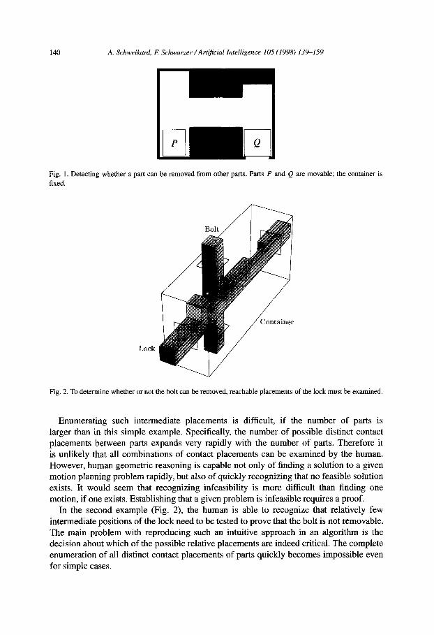
140 A. Schweikard, E Schwarzer/Artijicial Intelligence 105 (1998) 139-1.59

Fig. 1. Detecting whether a part can be removed from other parts. Parts P and Q are movable; the container is

fixed.

Fig. 2. To determine whether or not the bolt can be removed, reachable placements of the lock must be examined.

Enumerating such intermediate placements is difficult, if the number of parts is larger than in this simple example. Specifically, the number of possible distinct contact placements between parts expands very rapidly with the number of parts. Therefore it is unlikely that all combinations of contact placements can be examined by the human. However, human geometric reasoning is capable not only of finding a solution to a given motion planning problem rapidly, but also of quickly recognizing that no feasible solution

exists. It would seem that recognizing infeasibility is more difficult than finding one motion, if one exists. Establishing that a given problem is infeasible requires a proof.

In the second example (Fig. 2), the human is able to recognize that relatively few intermediate positions of the lock need to be tested to prove that the bolt is not removable. The main problem with reproducing such an intuitive approach in an algorithm is the decision about which of the possible relative placements are indeed critical. The complete enumeration of all distinct contact placements of parts quickly becomes impossible even for simple cases.

A. Schweikard, E Schwarzer/Art&ial Intelligence 105 (1998) 139-159 141

We are thus interested in methods for reducing the set of critical relative placements of parts, while retaining completeness. To obtain a practical method, it is necessary to recognize the essential contacts between parts. But notice that our detection of infeasibility would be in error if the set of examined contacts was too small.

In this context we will address the following problem:

Given an assembly of polygonal or polyhedral parts, decide whether one or more parts

can be removed from the remaining set of parts by an arbitrary sequence of translations.

Notice that we will restrict our attention to translational motion. This includes lock-and- key configurations, where several groups of parts must move simultaneously into distinct directions, and/or change direction during motion. The number of translations in such a sequence is not limited.

2. Related work

Toussaint [ 121 surveys earlier methods for separating sets in two and three dimensions. Applications in computer-aided design and medicine are considered in [5,6]. Agarwal, de

Berg, Halperin and Sharir [l] consider sequences of translations for separating polyhedra. In [ 1] the set of allowed motion directions is assumed to be given in advance. In [ 15 J the

concept of blocking graphs is introduced. This concept allows for deciding whether there is a subassembly S of a given assembly, such that S is removable by a single translation.

The output of the corresponding algorithm consists of S and a translational direction d for removing S, if there is such a subassembly S. This computation is possible in polynomial time, even though the number of removable subassemblies is exponential in general. The algorithm in [ 151 will thus compute a valid subassembly and a removal direction if there is

such a subassembly, but avoids enumerating the entire set of possible subassemblies. Specifically, the algorithm in [15] uses the following strategy. We pull on each of the

parts in turn with a series of given translational directions. For each direction in this set, we

compute the subset of parts which must follow the given pulling motion. Blocking graphs are used to compute this subset. The overall computing time is polynomial, since each translational direction can be analyzed in polynomial time, and the number of directions which must be analyzed is polynomial. This simple approach allows for several extensions (see, e.g., [4]), but inherently requires that all moving parts perform the same motion, and cannot be generalized to the case of multiple subassemblies moving independently.

Guibas and Halperin et al. [4] consider infinitesimal translations and rotations for partitioning three-dimensional sets. Such infinitesimal motions can indicate directions for removing parts in a single step. However, it cannot be guaranteed that the corresponding extended motion will be collision-free.

Pollack, Sharir and Sifrony [13] describe a near-optimal method for separating two polygons translating in the plane. The analysis in [ 131 is based on computing the boundary of a connected component in a two-dimensional arrangement. This connected component represents the set of placements reachable for the moving polygon. A generalization of the technique in [ 131 to the case of multiple moving polygons would compute the boundary of a connected component in a D-dimensional arrangement. An example in [3] provides

142 A. Schweikard, F: Schwarzer /Arrijicial Intelligence 105 (1998) 139-159

an exponential lower bound for the number of translations necessary to separate objects

(see also [ 111). This lower bound already holds for a restricted class of polygons in the plane. Interestingly, in special cases our technique allows for establishing infeasibility in

polynomial time, even if the boundary of the set of reachable placements has exponential

complexity. The next section gives an informal description of the basic principles in this context. The

main idea of the present approach is described in Section 4. Indeed, there is a remarkably simple way to compute certain multi-dimensional arrangements as arrangements of

surface patches, while avoiding the computation of the entire underlying arrangement

of hyperplanes. However, this is only possible for a particular class of arrangements. The arrangements to be considered here all belong to this class. Furthermore, we can

avoid computing the boundaries of connected components in the underlying arrangement.

As noted above, in special cases this allows for a complete search in polynomial time. Section 5 derives an algorithm from these principles and proves completeness. Section 6

describes a fast test for establishing whether a cell in a D-dimensional arrangement is bounded. Section 7 gives the analysis of the mentioned reductions. Section 8 describes

experimental results. The evaluation compares the derived methods with random motion

planners. The experiments suggest that it is possible to decide about infeasibility in a complete way. It is shown that the above principles lead to an exact algorithm of surprising performance in experiments.

3. Basic concepts

Let PI,..., Pk be an assembly of three-dimensional parts. Thus 9, . . . , Pk are nonintersecting polyhedra in given spatial placement. We allow for all parts to translate in

space independently. The position of each part is given by three parameters. A space ED of dimension D describes all simultaneous placements of all parts. Here D = 3k. A point in

this space is called forbidden if two or more parts intersect in the corresponding placement.

The origin in ED represents the initial placement of all parts and is not forbidden. We consider pairwise Minkowski-differences (C-obstacles, [S]) for each pair of parts

Pi, Pi. The C-obstacle for Pi and Pj is a three-dimensional region, defined by C( Pi, Pj) = {pi - pi 1 pi E Pi, pj E Pj}. The C-obstacles determine a set of halfspaces HI, _ . , , f& in ED, such that the forbidden regions are bounded by the corresponding hyperplanes in the following sense. HI, . . . , Hz determine an arrangement AD of halfspaces in ED, and partition ED into cells. A cell is a maximal connected region not containing any

points on any of the hyperplanes bounding HI, . . . , HS. Cells are thus open D-dimensional sets. Cells are regular, i.e., for each cell c either all or no points in c are forbidden. The

partitioning given by HI, . . . , H, also defines cells of dimension lower than D. Lower- dimensional cells are regular as well. (The construction of HI, . . . , Hs from the part set will be considered in more detail below.) Notice that AD contains unbounded ceils. An unbounded cell is a cell entirely containing a ray in its interior. A valid removal motion for one or more parts is a sequence of nonforbidden cells connecting the origin to one of the

unbounded cells.

A. Schweikard, E Schwarzer /Art$cial Intelligence 105 (1998) 139-159 143

A direct way to obtain an answer to the problem stated above is the following: we compute a graph representation of the arrangement AD [2]. Graph nodes for unbounded cells are labeled. Searching this graph will give an exact solution to the above problem. However, this direct method cannot be used in practice, because the graph representation of AD has an exponential number of nodes, and it is not possible to store this graph even for a small number of simple polyhedra.

To see whether parts are removable, it suffices to search a single connected component of the arrangement, namely the component containing the origin. It is obvious that searching only a single component will often reduce storage requirements to some extent, but this reduction is insufficient in practice. However, this simple idea provides a basis for a more effective reduction of search effort and storage requirements, described in the next section.

4. Floorgraphs

In the following we assume that all parts Pt , . . . , Pk are open sets. Thus placements

in which two parts are in contact, but do not overlap, are not regarded as intersections. Motions can consist of segments where two or more parts slide along each other. We also assume that all parts are bounded sets.

Constraintsforpairs ofparts. For two parts Pi and Pj, the bounding planes of C( Pi, Pj) define an arrangement of planes A(Pi, Pj) in three-dimensional space. We partition the complement of C( Pi, Pi) into convex regions. Each convex region thus obtained is given

as the intersection of halfspaces. Let Hy, . . . , Hj’ be the halfspaces stemming from Pi and Pj . These halfspaces are given as inequalities in the three parameters X, y and z.

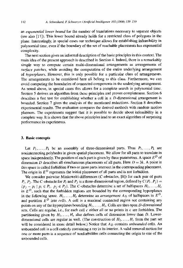
Let RI and R2 be two adjacent convex regions in the partitioning of the exterior of C( Pi, Pj). Then there is a cell c (of lower dimension) in the three-dimensional arrangement A( Pi, Pj) such that all points in R1 are visible from any point in c, and all points in R2 are

visible from any point in c (Fig. 3). We call c a passage or door cell. A j-loorgraph is defined in the following way. Each convex region in the above

partitioning of the exterior of C( Pi, Pj) corresponds to one node in the floorgraph. A door cell c shared by two regions RI and R2 defines an edge in the floorgraph. To each node/edge we assign a set of defining inequalities and equations.

Fig. 3. Door cell c. All points in both RI , R2 are visible from points in c.

144 A. Schweikard, E Schwarzer/Art@icial Intelligence 105 (1998) 139-159

Simultaneous motions of all parts. The D-dimensional arrangement AD is constructed

from the halfspace inequalities HI, . . . , Hs in the following way. The position of each part .

(i) Pi IS given by three parameters px , py (‘), pt) . These parameters describe the placement of

Pi with respect to the initial placement of Pi. Thus a point (p!l’ , py), pil), . . . , pik’, pik’,

pik’) describes a simultaneous placement of all parts PI, . . . , Pk. Each halfspace inequality Hi contains the three variables X, y and z. For an inequality

H stemming from a pair (Pi, Pj). we replace the variable x by the expression pt’ - pi”.

Similarly, we substitute pr’ - py’ for y and p!) - p6j’ for z. After this substitution, a pair

(Pj , Pi) gives the same inequalities as the pair (Pi, Pj). (This follows from the fact that

C( Pj, Pi) = -C(Pi, Pj) by definition.) Thus it is sufficient to consider each pair (Pi, Pj), wherei < j.

The inequalities are <-inequalities and not c-inequalities, because parts are open sets. We regard all inequalities thus obtained as D-dimensional inequalities, where at most six variables have nonzero coefficients.

The position of one (arbitrary) part must be fixed, since we are testing for removability. Otherwise all (D-dimensional) cells in A,g would be unbounded. We thus set the parameters pik’, pik’ and pik) of part Pk to zero.

Example 1. A simple assembly illustrates the above definitions (Fig. 4). In this example, we consider the two-dimensional case to simplify the description. The necessary modifi- cations of the definitions are straightforward. The assembly in Fig. 4 contains three parts P, Q, R. R is the (fixed) container. P and Q are rectangular. Here Q can only be moved

vertically. P can be translated arbitrarily. C( P, Q) is a rectangle (Fig. 5(a)). The exterior

p$ p-b start GOal

Fig. 4. Deciding whether a part can be removed from other parts. Part Q is constrained to move vertically only.

a) b) c)

Fig. 5. (a) Hyperplanes HI, . , H4 bounding C(P, Q). (b) Convex partitioning of the exterior of C(P, Q) into regions Ri. Door cell ‘12. (c) Floorgraph for pair (P. Q).

A. Schweikard, E Schwarzer/A@icial Intelligence 105 (1998) 139-159 145

a> b)

Fig. 6. (a) C-obstacle C( P, R) for parts P, R in Example 1. (b) Floorgraph for pair (P, R).

, I

‘. !

‘-,-,L _ ,‘I II

, , ’ ’

____ -__-. ‘\

‘. __--

-- ,

__-- _;,- I

‘\

*- ‘\ *- I , ‘8 ‘_)

, ,‘(I ‘\

I’ 2 ,’ ; I

\

,’

a) b)

Fig. 7. An arrangement of surface patches (a) has fewer cells than the corresponding arrangement of (extended)

hyperplanes (b) (c is a door cell).

of C(P, Q) is a union of halfspaces bounded by hyperplanes HI, . . . , H4. The orientations of HI, . . . , H4 are indicated by arrows in the figure.

By convention, the halfspace above Hi is denoted by Hi+. Hi- is the halfspace below Hi. The exterior of C(P, Q) is thus partitioned into four regions RI, . . . , R4, where RI, . . . , R4

are given by:

RI: H;“H;, R2: H; I-I H3-,

R3: H;nH,-, Rq: H4+ c-l HI-.

The floorgraph for C(P, Q) is shown in Fig. 5(c). The partitioning gives four door cells:

~-12: HI+ il Hz, ~3: H: fl H-3,

r34: H3+ n H4, r41: Hcfl HI.

The floorgraph for C(P, R) is shown in Fig. 6(b). Since we constrain Q to move vertically only, the floorgraph for (Q, R) can be represented by a single node Tt (not shown in the figure).

In the next section it will be shown that floorgraphs allow for searching AD in the following way:

146 A. Schweikard, E Schwarzer /Art$cial Intelligence 105 (1998) 139-159

l Only a single connected component within AD is traversed. We do not need to enumerate all free cells in AD.

l AD is searched as an arrangement of surface patches (Fig. 7), rather than an arrangement of full hyperplanes.

l The search avoids computing the boundaries of free connected components in AD.

5. Searching floorgraphs

In the above construction, one floorgraph corresponds to each pair of parts Pi, Pj where ic j.

Let GI,..., Gf be the floorgraphs thus obtained. Let nl , . . . , nf be nodes in the

floorgraphs, where ni is a node in Gi for each i. The tuple S = (nt , . . . , nf) will be called a D-node. Thus, a D-node contains exactly one node of each floorgraph. For a node n in one floorgraph, let C(n) be the set of defining constraint inequalities. Similarly C(e) gives the defining constraints for an edge e in one floorgraph. If x E ED satisfies the constraints

Chl>, . f. 3 C(nf) then S is called a feasible D-node. The D-nodes cover free space in ED, i.e., for each nonforbidden point a, there is a

D-node S = (nt, . . . , nf) such that a satisfies C(nt), . . . , C(nf). In particular, we can find a D-node for the origin in ED.

We define a successor of a D-node in the following way. Let

S=(nt,..., ni-1, ni, %+I,. . . , nf>

be a D-node. Then

S’=(Izr,..., I ni-l,ni,ni+l,..., nf)

is a successor of S, if ni is a successor of ni in the floorgraph Gi. Similarly, we define a successor-edge of a D-node:

S’= (nl, . . . . ni-l,e,ni+l, . . . . nf)

is a successor edge of

S=(nl,..., ni-i,ni,ni+i,...,nf)

if e is an edge emerging from ni in the floorgraph Gi . In general, a single D-node has several successors. Thus the successor relation on

D-nodes defines a graph. We search this graph in depth-first order, where all D-nodes previously visited are marked and not visited again:

(1) Compute all floorgraphs for pairs Pi, Pj with i c j.

(2) Compute a D-node S for the origin in ED.

(3) Set L = {S). (4) While L # empty

(a) Set P = first node in L and remove P from L. If P is unbounded, return the path from 0 to P and stop. Set L’ = successor edges of P.

(b) For each entry S in L’, test whether S is feasible. If so, store a point x satisfying the constraints in S, and a pointer from S to x . Otherwise, remove S from L’.

A. Schweikard, E: Schwarzer/Arti$cial Intelligence 105 (1998) 139-159 147

(c) Replace each successor edge in L’ by the corresponding successor node. Remove all previously visited nodes from L’. Insert all remaining entries of L’ at the front of L.

(5) If L = empty, return result ‘infeasible’, and stop. Notice that each intermediate point x stored with a D-node S (except the origin) is a

point in a door cell. Thus each point x computed in step 4(b) satisfies the constraints in one floorgraph edge and f - 1 floorgraph nodes. In step 4(c), the constraints for this edge are replaced by the constraints for the successor node in the corresponding floorgraph. New nodes generated at the initialization of the list L’ in step 4 again have constraints for f - 1

floorgraph nodes and one floorgraph edge. Segments of the paths can be contained entirely in cells of dimension less than D.

Let S = (n 1, . . , nf) be a D-node. In the remainder of this section we will regard S as a point set in E ‘, i.e., S is identified with the set of points satisfying the constraints in

C(nl ), . . . , C(~lf). Similarly, to simplify the notation, we will associate nodes and edges in floorgraphs with the corresponding point sets in E3.

We must show that the sequence of points thus computed indeed yields a feasible path.

Lemma 1. Let S1 be a feasible D-node and S2 be a feasible successor edge of SI . Let x1

be a point in Sl, and x2 be a point in S2. Then all points on the line se,qment connecting XI

to x2 in ED are in free space.

Proof. x1 is in a region defined by nodes n.1, . . . , nf . x2 satisfies the constraints

C(nt) U.. . U C(ni_1) U C(e) U C(ni+l) U . . . U C(nf),

where e is an edge emerging from ni in the floorgraph Gi Points satisfying C(e) also satisfy C(ni). Thus x2 satisfies

C(nl) U . . . U C(nj) U . . . U C(nf),

namely the constraints for xt. Each constraint set C(q) defines a convex set in ED, and their intersection is convex. Thus the entire line segment joining x1 and x2 is in free space. 0

Two D-nodes S and S’ will be called adjacent, if their intersection is nonempty.

Lemma 2. Let S = (nl, . . . , nf) and S’ = (n’,, . . . , n;) be two adjacent D-nodes. Then

for each i with ni # n:, the nodes ni and ni are connected by an edge e in thejoorgraph

G;. Both C(nl) , . . . , C(ni-I), C(e), C(ni+l), . . . , C(n,f) and C(n;), . . . , C(n:_,), C(e). C(ni+,), . . , C(n)) are feasible.

Proof. We require that the (3D) partitioning of the exterior of each C-obstacle be such that two distinct regions have disjoint interiors. Thus all points in the intersec- tion of two floorgraph nodes are points in door cells. Assume, pri # ni. If ni n ni

is empty, then S n S’ is also empty, contradicting the adjacency of S and S’. Thus ni and ni are connected by an edge e in Gi. Let x be in S n S’. Then x satis- fies both C(nl), . . ., C(nf) and C(n’,), . . . . C(n>). All points satisfying both C(ni)

148 A. Schweikard, E Schwarzer /Artificial Intelligence 105 (1998) 139-159

and C(ni) also satisfy C(e), due to the above property of the three-dimensional par- titioning. Thus x satisfies C(nr), . . ., C(ni_r),C(e), C(nj+l), . . ., C(nf) as well as

C(Q,. . ., C(n~_,>, C(e), C(n:+l), . . . , CC+). 0

The completeness of the above method follows from Lemma 3:

Lemma 3. Let u be a continuous path connecting the origin to an unbounded cell, such

that all points on u are in free space. Then there is a sequence Tl , . . . , Tr of D-nodes,

which covers u, such that Tj+l is a successor of Tj in the search graph.

Proof. The D-nodes cover free space in ED. Thus u traverses a sequence St, . . . , S, of D-nodes, covering u. Let j < r. The D-nodes are closed sets so that, due to the continuity of the path, Sj II Sj+t is nonempty, i.e., Sj and Sj+r are adjacent.

We must show that Sj+t will be expanded, once Sj has been expanded. Thus it remains to be shown that Sj+l is either a direct successor of Sj in the search graph, or Sj and Sj+l

are connected by a chain of feasible D-nodes in this graph. LetSj=(nl,..., nf)andSj+l=(n;,..., n;). Assume nl # ni. By Lemma 2, n1 and

n; are connected by an edge e, and C(e), C(nz), . . . , C(nf) is feasible. Thus the D-node

S(l) defined by St’) = (n;, 122, . . . , nf) is feasible. SC’) is a successor of Sj, since it is

connected to Sj by the (feasible) edge e.

Since Sj to Sj+t are adjacent, there is a point x satisfying both C(nl), . . . , C(nf) and

C(n;), . . . , C(n)). Thus x satisfies C(n;), C(nz), . . . , C(nf), i.e., the constraints for S(l).

But then x is a common point of S(l) and Sj+t, so that S(l) is adjacent to Sj+r. Thus we can apply the same argument to the pair n2, n;. If n2, n; are distinct, then the D-node

Sc2) = (nl,, n;, ng, . . . , nf) is feasible and adjacent to Sj+t . Furthermore Sc2) is a successor

of S(l). Repeating this replacement step at most f times, we obtain a sequence of D-nodes connecting Sj to Sj+l in the search graph via a chain of feasible edges. q

Remark. Let n and n’ be two nonadjacent nodes in one floorgraph G. The constraint hyperplanes in n do not partition the region corresponding to n’ and vice versa. Similarly,

a door cell between two regions is a patch, not intersecting regions determined by other nodes in G. In this sense, the regions in AD corresponding to floorgraph nodes are bounded

by surface patches rather than full hyperplanes.

6. Implementation

To obtain a practical algorithm, we must implement the test for feasibility in step 4(b) of the above algorithm. This test is implemented as a linear feasibility test [lo]. If positive, the test returns a point x satisfying the given constraints. In the feasibility test, we must

ensure that variables may become negative. Here standard methods apply. Furthermore, we must implement the test for boundedness in step 4(a) to decide whether

the current D-node contains a ray u. Let S be this D-node. u may have points in the

A. Schweikard, E Schwurzer /Arti&ial Intelligence 105 (1998) 139-159 149

boundary of S, i.e., on the defining hyperplanes of S, but must not cross these hyperplanes.

Let

HI: alx - dl = 0, . . . , Hr: a,x - d, = 0

be the equations of the hyperplanes defining S. al, . . . , a, are the normal vectors of the

hyperplanes HI, . . . , Hr. Let xc be the point in S computed in step 4(b). Assume these hyperplane equations are oriented such that x0 is above (or in) all hyperplanes HI, . . . , Hr, i.e., alx~ - dl 3 0, _ _ . , a,xo - d, 2 0. To decide whether there is a vector u such that

xe + tu does not cross one of HI, . . . , H,. for any t > 0 it suffices to test whether there is a

nonzero vector u with alu 3 0, . . . , a,u > 0. Let d # 0 and H: ax - d = 0 be an arbitrary hyperplane. Then H’: ax + d = 0 is

parallel to H. Since d # 0, both H and H’ do not contain the origin. To find u we use

two linear feasibility tests. The first test determines whether there is a u with au - d = 0, al u 3 0, . . , a,u 3 0. The second test determines whether there is a u with au + d = 0, alu > 0,. . . , aru 3 0. As above, in both tests we must allow for coordinates of u to

become negative. S is unbounded if one of the tests succeeds. However, the test may fail to detect unboundedness. This case occurs if the set of all vectors u representing valid removal directions is entirely contained in the hyperplane ax = 0. We can ignore this case,

for the following reason: all parts are bounded. Thus free space in ED contains a single

unbounded component. The unbounded component contains at least one D-node with full

dimension D This simple test assumes bounded parts. A more detailed analysis shows that the

latter restriction can be removed. Generally, a single linear range computation followed by a single linear feasibility test is sufficient for establishing whether a given cell is

unbounded [ 141.

7. Analysis

The above algorithm outputs a path-if one exists-as a sequence of line segments in ED. Each segment represents a simultaneous translation of one or more parts, possibly in

distinct directions. To find such a path, a tree of cells is expanded. We will first consider the number of node expansion steps for generating this tree. We

decompose the faces of each part into triangles. Let n be the maximum number of triangles

in each of the k parts. Then n is a bound for the number of vertices of each part. To compute the pair-wise Minkowski-differences, it suffices to compute the Minkowski-differences for

pairs of triangles on faces, and we then obtain O(n2) inequalities for each pair of parts. The number of such pairs is bounded by k2, so that we obtain a total of O(k2n2) halfspaces in AD. Each step will reach a new cell in AD, since each step reaches a yet unvisited D-node,

and crosses at least one hyperplane at the same time. It is well known that an arrangement of u hyperplanes in D dimensions has at most

O(uo) cehs, including cells of lower dimension (see, e.g., [2]). Tbus AD has at most 0((k2n2)D) cells. Here D = 3k - 3 for polyhedral assemblies and D = 2k - 2 in the

planar case.

1.50 A. Schweiknrd, F: Schwarzer/Artijicial Intelligence 105 (1998) 139-159

Lemma4 The number of node expansions in the above algorithm is bounded by 0(k2DmD), where m is the maximum number of nodes in a connected component of a

floor-graph and k is the number of parts.

Proof. Each node in each floorgraph represents a convex (generalized) cylinder in ED.

(The cylinders are called generalized cylinders because their bounding surfaces are linear, not curved, so that the cylinders are prisms with convex base.) The set of feasible points for a D-node is the intersection of 0(k2) such cylinders. At each step, we proceed from one convex cell of this cylinder arrangement to the next convex cell. Notice that the cylinder arrangement contains non-convex cells as well. At most one unbounded D-node will be examined, so we must only account for bounded nodes. There is a vector v in ED such that each bounded convex cell has exactly one extremal vertex in direction u. Each vertex is the intersection of exactly D hyperplanes, except in cases where hyperplanes are not in general position. After a sufficiently small displacement of all hyperplanes, we can reach a placement in which each u-extremal vertex is the intersection of exactly D distinct

hyperplanes. This displacement of each hyperplane can be made sufficiently small so that none of the convex cells of the cylinder arrangement will vanish. Therefore we can assume that the number of convex cells will not be decreased by the displacement. Of course, the displacement is only done for accounting purposes, not by the program.

Each v-extremal vertex of each convex cell is the intersection of, at most, D cylinders. There are O(k2m) cylinders. We consider the number of subsets with, at most, D elements in this set of size O(k2m). This number is bounded by

where e is the Euler constant. The first step in this chain of inequalities is the least obvious,

but becomes clear if we observe that for any a 3 i

a 0 1 . . . . . (a - i)(a - i + 1). . . . . a =

i i!.(l.....(a-i)) <;.

Thus there are O((k2m)D) extremal vertices of convex cells in the cylinder arrangement.

Each such convex cell has one v-extremal vertex, i.e., there are 0((k2m>D) convex cells in the cylinder arrangement. 0

Since k and D are related, the above bound on the number of node expansions can be reduced: in the following we consider only the case of three-dimensional assemblies.

Lemma 5. There is a constant Do such that the number of node expansions in the above algorithm is bounded by O(kf(D)mg(D)), wh ere f and g arefunctions with f(D) < D and

g(D) < D for any D larger than Do.

Proof. From the proof of the previous lemma, the expression

A. Schweikard, E Schwarzer /Artificial Intelligence 105 (1998) 139-159 1.51

is a bound for the number of node expansion steps. As noted in Section 4, the pair (Pi, Pj) of parts will give rise to the same constraints as the pair (Pj , Pi). Therefore we must only consider ordered pairs of parts (Pi, Pi) where i -c j, i.e., the total number of floorgraphs is bounded by k2/2. Then the value

equally bounds the number of node expansions. If k is sufficiently large, we have 20 < k2m/2, since D = 3k - 3.

By an elementary property of binomial coefficients, the values in a sequence of the form (t) , . . . , (;) grow monotonically, as long as 2 j < n.

Therefore

for each i = 1, . . . , D, if k is sufficiently large. Then

and by Stirling’s formula,

mD q<D-

k2’

2O &DDe-D’

Rearranging gives

With

,f (D) = 20 - D”;,“,, ’ +i and g(D)=D(l-E)

we can finally write q = O(kf(D)mg(D)).

In the three-dimensional case D = 3k - 3. Therefore (log D - l)/logk > 1 for sufficiently large k and D, so that f(D) < D and g(D) < D. •I

From the number of expansion steps, one can obtain a bound for the running time of the algorithm: let LP(s, D) be the number of steps required for solving a linear program with s constraints and D variables. Then each node expansion requires at most 0((k2r)LP(k2r, D)) steps, where r is the maximum number of constraints in each floorgraph. The total running time is thus bounded by 0((k2m)Dk2rLP(k2r, D)).

In this bound we have not accounted for the precomputation of pairwise floorgraphs. The analysis of this preprocessing step is straightforward and follows methods in [ 1 l] and [ 151.

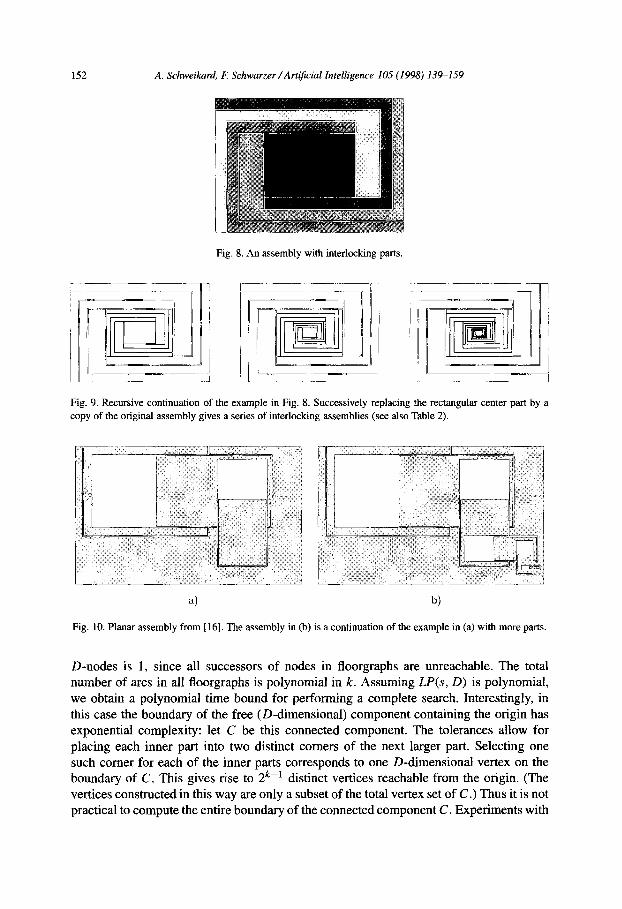
Remark 1. The parts in Fig. 8 interlock. A series of similar assemblies with growing number k of parts is shown in Fig. 9. Here m > 1. However, the total number of examined

152 A. Schweikard, E Schwarzer /Arti$cial Intelligence IO5 (1998) 13%159

Fig. 8. An assembly with interlocking parts.

1 L,__ --d _ IrEx:--.-- -.I

Fig. 9. Recursive continuation of the example in Fig. 8. Successively replacing the rectangular center part by a

copy of the original assembly gives a series of interlocking assemblies (see also Table 2).

4 b)

Fig. 10. Planar assembly from [ 161. The assembly in (b) is a continuation of the example in (a) with more parts.

D-nodes is 1, since all successors of nodes in floorgraphs are unreachable. The total number of arcs in all floorgraphs is polynomial in k. Assuming L&s, D) is polynomial, we obtain a polynomial time bound for performing a complete search. Interestingly, in this case the boundary of the free (D-dimensional) component containing the origin has exponential complexity: let C be this connected component. The tolerances allow for

placing each inner part into two distinct comers of the next larger part. Selecting one such comer for each of the inner parts corresponds to one D-dimensional vertex on the boundary of C. This gives rise to 2k-’ distinct vertices reachable from the origin. (The vertices constructed in this way are only a subset of the total vertex set of C.) Thus it is not practical to compute the entire boundary of the connected component C. Experiments with

A. Schweikard, E Schwarzer /Art$cial Intelligence 105 (1998) 139-159 153

the examples in Fig. 9 illustrate the growth of the computing time with growing number k of parts (see Table 2 in the next section).

The above remark does not only apply to infeasible assemblies. An example of a feasible assembly is shown in Fig. 10. In this case, the complexity of the cell containing the origin

is exponential as well (the boundary of this cell has an exponential number of vertices). However, the number of node expansions is only linear in the number of parts which results in a polynomial overall running time.

8. Experiments

To find practical limitations, the above algorithm was implemented for the planar case on a Unix-workstation HP 700 in C++ based on the LEDA-library [9]. Integer arithmetic

was used in the preprocessing steps, and simplex linear programming was used for the feasibility tests.

8.1. Simple examples

Figs. 1 l(a)-(c) show three simple examples (see also Table 1). In Fig. 1 l(b), a sliding motion is required for separating the parts. Specifically, the two center parts have total length equal to the width of the container opening. (All coordinates are integers.) Therefore the system must find and traverse a channel of width zero in the set of feasible placements to remove a part in case (b).

b)

Fig. 11. Simple examples.

154 A. Schweikard, E Schwarzer/Artijicial Intelligence 105 (1998) 139-159

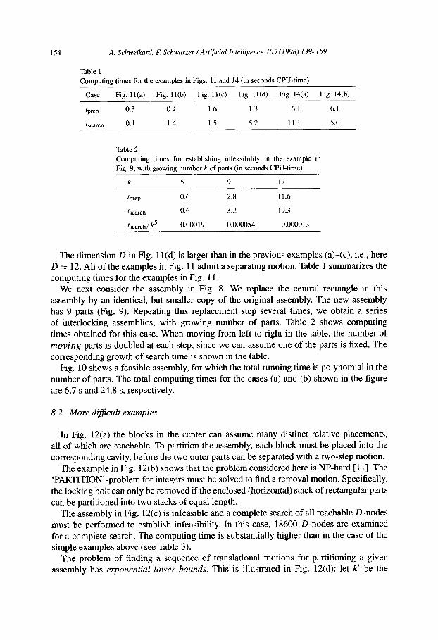
Table 1

Computing times for the examples in Figs. 11 and 14 (in seconds CPU-time)

Case Fig. 1 l(a) Fig. 11 (b) Fig. 11(c) Fig. 11(d) Fig. 14(a) Fig. 14(b)

tP=P 0.3 0.4 1.6 1.3 6.1 6.1

kearch 0.1 1.4 1.5 5.2 11.1 5.0

Table 2

Computing times for establishing infeasibility in the example in

Fig. 9, with growing number k of parts (in seconds CPU-time)

k 5 9 17

tP=P 0.6 2.8 11.6

&arch 0.6 3.2 19.3

kearch I k5 o.oOQ19 0.000054 0.000013

The dimension D in Fig. 1 l(d) is larger than in the previous examples (a)-(c), i.e., here D = 12. All of the examples in Fig. 11 admit a separating motion. Table 1 summarizes the computing times for the examples in Fig. 11.

We next consider the assembly in Fig. 8. We replace the central rectangle in this assembly by an identical, but smaller copy of the original assembly. The new assembly has 9 parts (Fig. 9). Repeating this replacement step several times, we obtain a series of interlocking assemblies, with growing number of parts. Table 2 shows computing times obtained for this case. When moving from left to right in the table, the number of

moving parts is doubled at each step, since we can assume one of the parts is fixed. The corresponding growth of search time is shown in the table.

Fig. 10 shows a feasible assembly, for which the total running time is polynomial in the number of parts. The total computing times for the cases (a) and (b) shown in the figure

are 6.7 s and 24.8 s, respectively.

8.2. More difJicult examples

In Fig. 12(a) the blocks in the center can assume many distinct relative placements, all of which are reachable. To partition the assembly, each block must be placed into the corresponding cavity, before the two outer parts can be separated with a two-step motion.

The example in Fig. 12(b) shows that the problem considered here is NP-hard [l 11. The ‘PARTITION’-problem for integers must be solved to find a removal motion. Specifically,

the locking bolt can only be removed if the enclosed (horizontal) stack of rectangular parts can be partitioned into two stacks of equal length.

The assembly in Fig. 12(c) is infeasible and a complete search of all reachable D-nodes must be performed to establish infeasibility. In this case, 18600 D-nodes are examined

for a complete search. The computing time is substantially higher than in the case of the simple examples above (see Table 3).

The problem of finding a sequence of translational motions for partitioning a given assembly has exponential lower bounds. This is illustrated in Fig. 12(d): let k’ be the

A. Schweikard, E Schwarzer /Artificial Intelligence 105 (I 998) 139-l-159

il

Fig. 12. More difficult examples. Example in (b) is feasible, (c) is infeasible.

Table 3 Computing times for the examples in Fig. 12 (in seconds CPU-time). Second line: search

times with modified ordering of node expansions (nodes with largest distance from the

origin are expanded first)

Case Fig. 12(a) Fig. 12(b) Fig. 12(c) Fig. 12(d)

t (depth-first search) 1380 19910 20180 1386

t (heuristic expansion ordering) 12.9 35.7 20193 18.3

number of u-shaped parts in the figure. If k’ is sufficiently large, we must follow a

variant of the rules for the Towers of Hanoi in order to remove a part 131. The number of distinct translational motions (i.e., motions with distinct directions or distinct part sets) for removing a part is exponential in k’. The computing times for the example in Fig. 12(d)

are shown in the last column of Table 3. Feasible problems can be solved more rapidly if the D-nodes are not expanded in an

uninformed depth-first order. A very simple modification is to use a heuristic search where the node with largest distance to the origin (among new nodes) is always expanded first. The second line of Table 3 shows computing times obtained with this modification. Notice

156 A. Schweikard, E Schwarzer/Art$cial Intelligence 105 (1998) 139-159

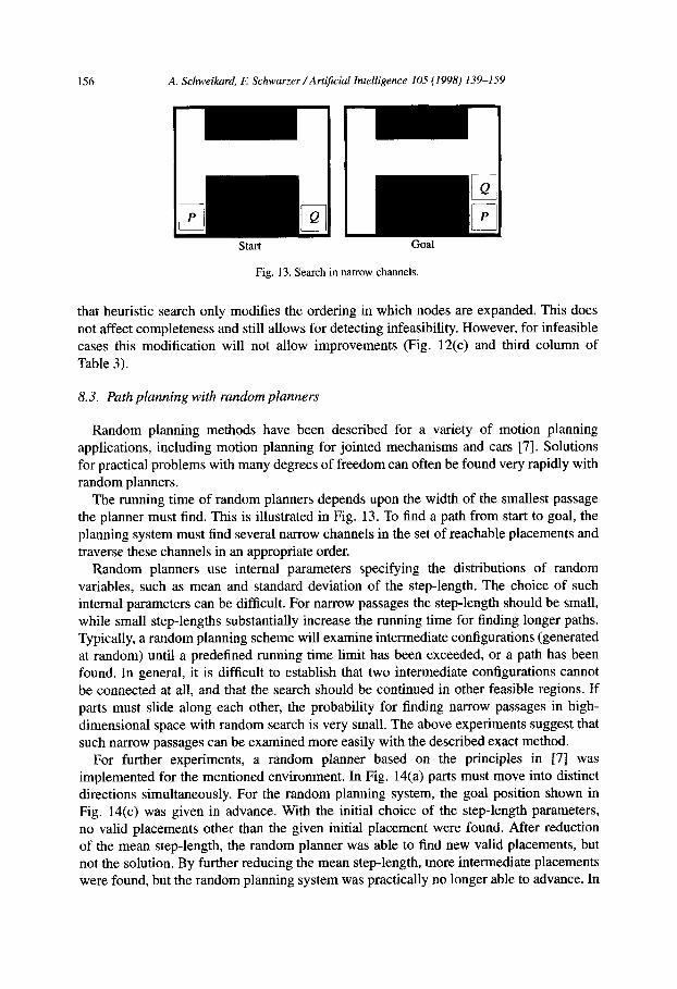
Fig. 13. Search in nanow channels.

that heuristic search only modifies the ordering in which nodes are expanded. This does not affect completeness and still allows for detecting infeasibility. However, for infeasible cases this modification will not allow improvements (Fig. 12(c) and third column of

Table 3).

8.3. Path planning with random planners

Random planning methods have been described for a variety of motion planning applications, including motion planning for jointed mechanisms and cars [7]. Solutions for practical problems with many degrees of freedom can often be found very rapidly with random planners.

The running time of random planners depends upon the width of the smallest passage the planner must find. This is illustrated in Fig. 13. To find a path from start to goal, the planning system must find several narrow channels in the set of reachable placements and

traverse these channels in an appropriate order. Random planners use internal parameters specifying the distributions of random

variables, such as mean and standard deviation of the step-length. The choice of such internal parameters can be difficult. For narrow passages the step-length should be small, while small step-lengths substantially increase the running time for finding longer paths. Typically, a random planning scheme will examine intermediate configurations (generated at random) until a predefined running time limit has been exceeded, or a path has been found. In general, it is difficult to establish that two intermediate configurations cannot be connected at all, and that the search should be continued in other feasible regions. If parts must slide along each other, the probability for finding narrow passages in high-

dimensional space with random search is very small. The above experiments suggest that such narrow passages can be examined more easily with the described exact method.

For further experiments, a random planner based on the principles in [7] was implemented for the mentioned environment. In Fig. 14(a) parts must move into distinct directions simultaneously. For the random planning system, the goal position shown in Fig. 14(c) was given in advance. With the initial choice of the step-length parameters, no valid placements other than the given initial placement were found. After reduction of the mean step-length, the random planner was able to find new valid placements, but not the solution. By further reducing the mean step-length, more intermediate placements were found, but the random planning system was practically no longer able to advance. In

A. Schweikard, F: Schwarzer/Am$cial Intelligence IO5 (1998) 139-159 157

b)

Fig. 14. Testing for removability of parts. (a) Removal motion exists. (b) No removal motion. (c) Goal position

for the random planner.

Figs. 14(a), (b) the running times for the exact method were 17.2 s and 11.1 s, respectively. Notice that the example in Fig. 14(b) is infeasible. The computing time in case (b) is

smaller than in case (a), since the set of reachable D-nodes is more restricted than in case (a).

8.4. Further examples

The problem of m-handed assembly planning is stated as follows: decide whether parts in a given assembly can be separated by a single translation, where parts or subassemblies may move into distinct translational directions. Here m denotes the number of subassemblies moving into distinct directions. The assembly in Fig. 1 l(a) can be partitioned with such a single-step motion.

After small modifications, the program can be used to decide whether a given assembly admits an m-handed assembly sequence. For planar parts it can be shown that this computation can always be performed in polynomial time if no pair of parts is separated

by a line in the initial configuration [ 141. Interestingly, the assembly in Fig. 15 allows for three-handed assembly which is

established by the program in less than 0.1 s. The program also establishes that no two- handed assembly motion exists in this case. For the human it is not obvious that the parts

in this figure can be separated by a singEe three-handed translation. The intuitive approach would be to move one pair of adjacent parts (vertically or horizontally) until a contact with one of the other parts occurs. Then one would select a different pair and remove it with a translation perpendicular to the first, which is possible from the intermediate placement. Finding a single translation (i.e., a three-handed motion) in this case is left to the reader.

158 A. Schweikard, E Schwarzer/Art$cial Intelligence 105 (1998) 139-1.59

Fig. 15. m-handed assembly planning.

9. Conclusions

In special cases, the proposed graph representation allows for a complete search in polynomial time, even if the boundary of the free component has exponential complexity.

A direct way to include heuristics into the search process (while retaining completeness) is to modify the ordering in which D-nodes are expanded. Experiments suggest that appropriate heuristics can reduce search times. However, heuristics can only give improvements for feasible assemblies.

In the experiments, computing times for establishing infeasibility are substantially

shorter, if the set of reachable D-nodes is small. This appears to be the case for tight assemblies in particular and suggests that the above approach is more suitable for applications in assembly planning than for general motion planning.

Assembly motions requiring many changes of directions or velocities increase assembly costs, and are often impractical due to fixturing and stability problems. From a practical point of view, finding one assembly motion-if there is such a motion-is the main objective of planning methods. In this context it seems useful to fix an upper bound for the number of allowed changes in direction/velocity of parts. The number of D-nodes along a path bounds the number of direction/velocity changes during the motions. However, the direct computation of paths with minimum number of direction/velocity changes has not yet been explored in the context of the above methods.

Acknowledgements

The authors thank Florian Bieberbach, Akos Czopf, Leo Joskowicz and Randy Wilson for comments and discussions.

References

[I] P.K. Agarwal, M. de Berg, D. Halperin, M. Sharir, Efficient generation of k-directional assembly sequences,

in: Proceedings 7th ACM-SIAM Symp. Discrete Algorithms (SODA), 1996, pp. 122-131. [2] H. Edelsbrunner, Algorithms in Combinatorial Geometry, Springer, Heidelberg, 1987. [3] B. Chazelle, T.A. Ottmann, E. Soisalon-Soininen, D. Wood, The complexity and decidability of SEPARA

TION, in: Proceedings 1 lth International Colloquium on Automata, Languages, and Programming, Lecture

Notes in Comput. Sci., Vol. 172, Springer, Berlin, 1984, pp. 119-127.

A. Schweikard, E Schwarzer/Art$cial Intelligence 105 (1998) 139-159 159

]4] L. Guibas, D. Halperin, H. Hirukawa et al., Polyhedral assembly partitioning using maximally covered cells

in arrangements of convex polytopes, Intemat. J. Comput. Geometry and Applications (to appear).

[5] L.S. Homem de Mello, A.C. Sanderson, Automatic generation of mechanical assembly sequences, Technical

Report CMU-RI-TR-8% 19, Robotics Institute - Carnegie-Mellon University, Pittsburgh, PA, 1988.

[6] L. Joskowicz, R.H. Taylor, Interference-free insertion of a solid body into a cavity: an algorithm and a

medical application, Intemat. J. Robotics Research 15 (3) (1996).

171 J.-C. Latombe, Robot Motion Planning, Kluwer Academic Publishers, Boston, 1991.

[S] T. Lozano-Perez, Spatial planning: a configuration space approach, IEEE Trans. Comput. C-32 (2) (1983)

108-120.

[9] K. Mehlhom, S. Naeher, LEDA: A Platform for Combinatorial and Geometric Computing, Max-Planck-

Institut fttr Informatik, Saarbrtlcken, 1995.

[lo] J.J. More’, S.J. Wright, Optimization software guide, SIAM J. Frontiers in Appl. Math. 14 (1993). See also:

http:Nwww.mcs.anl.govlhomelotc/Guide/Softw~eGuide/.

[ 1 l] J. O’Rourke, Computational Geometry, Cambridge University Press, Cambridge, 1994.

[ 121 G.T. Toussaint, Movable separability of sets, in: G.T. Toussaint (Ed.), Computational Geometry, Elsevier,

North Holland, Amsterdam, 1985.

[13] R. Pollack, M. Sharir, S. Sifrony, Separating two simple polygons by a sequence of translations, Discrete

Comput. Geom. 3 (1988) 123-136.

[14] E Schwarzer, F. Bieberbach, L. Joskowicz, A. Schweikard, Efficiently testing for unboundedness and I)Z-

handed assembly, Technical Report TUM-19750, Informatik, TU Mtinchen, 1997.

[15] A. Schweikard, R.H. Wilson, Assembly sequences for polyhedra, Algorithmica 13 (6) (1995) 539-552.

[ 161 J.D. Walter, On the automatic Generation of Plans for Mechanical Assembly, Ph.D. Thesis, University of

Michigan, Ann Arbor, MI, 1988.