Detecting Earnings Management Using Discontinuity … · Detecting Earnings Management Using...

Detecting Earnings Management Using Discontinuity Evidence*

David Burgstahler Julius A. Roller Professor of Accounting

University of Washington/Seattle

Elizabeth Chuk Assistant Professor

University of Southern California

January 20, 2014

Abstract

Evidence of earnings management based on discontinuities in earnings distributions at prominent benchmarks is pervasive, yet there is little evidence of significant abnormal accruals in settings where there is clear evidence of earnings management to meet benchmarks. Together with previous results on the characteristics of accruals-based tests, results in this paper on the statistical characteristics of discontinuity tests reconcile this apparent inconsistency. The distribution of the standardized difference statistic is derived, relaxing the Burgstahler and Dichev (1997) assumption that the two components in the numerator of the standardized difference are independent. Simulation results confirm the derivation and also suggest that the independence assumption is not likely to induce important errors in typical applications. The power of the standardized difference test is evaluated for alternative assumptions about the pattern of earnings management to meet benchmarks. In contrast to results from previous research that suggest abnormal accruals tests have reasonable power only in samples where there are high rates and large amounts of accruals management, discontinuity tests have the power to detect far smaller amounts and much lower rates of total earnings management to meet a benchmark.

Preliminary and incomplete draft prepared for discussion at UTS. Comments invited but please do not quote, cite, or distribute without permission

JEL classification: G14, M40 Key Words: Earnings management, discontinuities

* We appreciate helpful comments and suggestions from Russell Lundholm, Norman Strong, and seminar participants at the University of British Columbia and the University of Illinois.

1. Introduction

There is pervasive evidence of discontinuities in distributions of reported earnings at

prominent earnings benchmarks, where distributions comprise fewer observations immediately

below the benchmark and more observations immediately above the benchmark than would be

expected if the distribution were smooth.1 The body of evidence is consistent with the theory

that managers take actions to ensure that earnings meet benchmarks, e.g., earnings are managed

to avoid small losses, small earnings decreases, and small negative earnings surprises.2 This

interpretation is further supported by survey evidence in Graham, Harvey, and Rajgopal (2005)

indicating that managers are willing to incur real costs in order to meet benchmarks. However,

there has been no formal evaluation of the statistical properties of discontinuity tests to detect

earnings management.3

Inferences from empirical evidence depend on an understanding of the determinants of

the size and power of the statistical tests employed. If a test is sensitive to violations of

assumptions, a significant test statistic might be attributable to violations of assumptions rather

than to a false null hypothesis. On the other hand, if a test has low power, insignificant results

might be attributable to low power rather than to a true null hypothesis. Further, significant

results from a test with low power lead to little or no revision in beliefs.4

1 The smoothness assumption is discussed in more detail in Section 2. 2 For example, Burgstahler and Dichev (1997, hereafter BD) show that distributions of earnings levels and distributions of earnings changes exhibit discontinuities at zero and there is widespread evidence of discontinuities in distributions of earnings surprises, e.g., Degeorge, Patel, and Zeckhauser (1999), Brown (2001), Matsumoto (2002), Brown and Caylor (2005), Burgstahler and Eames (2006). There is also evidence of discontinuities at prominent non-zero earnings benchmarks, e.g., Carslaw (1988), Thomas (1989), Das and Zhang (2003), Grundfest and Malenko (2009), and Burgstahler and Chuk (2013). 3 In contrast, the power of methods of detecting earnings management based on measures of abnormal accruals is evaluated in Dechow, Sloan, and Sweeney (1995), Dechow et al (2010), and Ecker et al (2011). 4 See Burgstahler (1987) for further discussion of the roles of size and power in inference from empirical results.

The purpose of this paper is to (i) refine the derivation of the distribution of the

Burgstahler and Dichev (1997, hereafter BD) standardized difference statistic under the null and

alternative hypotheses, relaxing the BD simplifying assumption that the two numerator

components of the test statistic are independent, and (ii) analyze the determinants of the power of

standardized difference tests under various alternative hypotheses, i.e., various assumptions

about how earnings are managed to meet benchmarks.

The power analysis shows that the standardized difference test has power to detect

management of relatively small amounts of earnings by even a small proportion (such as .25–

.50% of MVE for .1-.2%) of sample firms.5 In contrast, previous research suggests that accruals-

based tests have reasonable power only for much larger amounts and much higher rates of

earnings management. Thus, discontinuity tests have far greater power to detect much less

pervasive, and much smaller amounts of, earnings management than do tests based on abnormal

accruals. These results reconcile what has sometimes been interpreted as an inconsistency in the

literature, namely the absence of significant abnormal accruals among firms with earnings that

fall just above significant benchmarks (Dechow, Richardson, and Tuna 2003, Ayers et al 2006).

The paper is organized as follows. Section 2 provides background. Section 3 reviews

and refines the theoretical derivation of the distribution of the standardized difference statistic.

Section 4 provides simulation evidence to confirm the derivation. Section 5 analyzes the

determinants of power of the standardized difference test and discusses implications for research

design. Section 6 concludes.

5 As explained further below, .1%-.2% is the proportion of firms managing earnings when, for example, 1% of the population has pre-managed earnings a small amount below a benchmark and 10%-20% of firms with earnings a small amount below a benchmark manage earnings upwards to meet the benchmark.

2. Background

Earnings management occurs when the perceived benefits of managing earnings

(including both benefits to the firm and potentially divergent benefits to the manager) exceed the

costs. Healy and Wahlen (1999) note: "Despite the popular wisdom that earnings management

exists, it has been remarkably difficult for researchers to convincingly document it." There is

pervasive evidence of discontinuities in earnings distributions at prominent benchmarks,

consistent with earnings management.6 In contrast, there is less evidence of significant abnormal

accruals in situations where earnings management behavior is hypothesized. Further, Ball

(2013) outlines a number of reasons to be skeptical about significant abnormal accruals results

that imply that management of “enormous amounts” of accruals is “rife.”

2.1 Evidence of discontinuities

Earnings management to meet a benchmark transforms some pre-managed earnings

observations below the benchmark into reported (i.e., post-managed) observations above the

benchmark.7 The result is a decrease in the frequency of earnings observations below the

benchmark and an increase in the frequency above the benchmark, creating a discontinuity at the

benchmark in the distribution of reported (post-managed) earnings.8

The set of alternative methods of earnings management is broad. To meet a benchmark,

managers might enter into real operating, investing, or financing transactions that generate

6 Two recent papers by Durtschi and Easton (2005 and 2009) purport to show that the discontinuities in earnings distributions are explained by “deflation, sample selection, and a difference between the characteristics of profit and loss observations.” Burgstahler and Chuk (2013) show that the Durtschi and Easton "explanations" for discontinuities are erroneous. 7 Researchers have examined incentives to manage earnings upward to create the appearance of better current performance, or downward to create the appearance of worse current performance or to transfer earnings to future periods from the current period. This paper focuses on upward management to increase current performance, the phenomenon that creates discontinuities at current earnings benchmarks. 8 Kerstein and Rai (2007) provide direct evidence that earnings management converts observations below the benchmark into observations above the benchmark.

additional current profits, where these transactions might be purely incremental with no effects

on future profitability or they might have adverse effects on future profitability.9 In addition,

managers might make accounting choices to increase current reported profits. For example,

managers might accelerate recognition of revenues or defer recognition of expenses as permitted

within GAAP. Managers might record transactions in a way that violates GAAP or record

fictitious or fraudulent transactions. Any combination of these actions can be used to manage

earnings to meet the benchmark, and managers are expected to choose the lowest-cost

combination. Because reported earnings reflect all of these actions, discontinuities provide

evidence that some combination of these actions has been taken to meet the benchmark, but do

not reveal which actions were taken.10

Multiple studies document discontinuities around various earnings benchmarks, including

the profit/loss benchmark (Hayn, 1995; BD, 1997; Degeorge et al., 1999); prior-year earnings

(BD, 1997; Degeorge et al., 1999; Beatty et al., 2002; Donelson et al., 2013); and analyst

forecasts (Degeorge et al., 1999; Burgstahler and Eames, 2006; Donelson et al., 2013). Leuz,

Nanda, and Wysocki (2003) report evidence of loss avoidance for an international sample of

firms from 31 countries. Suda and Shuto (2005) provide strong evidence that Japanese firms

engage in earnings management to avoid earnings decreases and losses. Haw et al. (2005)

document discontinuities for the return on equity (ROE), where there is an unusually high

proportion of firms reporting ROEs slightly greater than the 10% benchmark. Daske, Gebhardt,

9 See Jensen (2001, 2003) for multiple examples of transactions and decisions that increase current earnings but decrease expected future earnings and firm value. 10 Schipper (1989) defines "disclosure management" as "purposeful intervention in the external financial reporting process, with the intent of obtaining some private gain…"(p. 92) but also notes that there are additional forms of "real" earnings management. i.e. real operating, investing, or financing decisions that alter reported earnings. Healy and Whalen (1999) use a broad definition that encompasses a broad range of actions: "Earnings management occurs when managers use judgment in financial reporting and in structuring transactions to alter financial reports to either mislead some stakeholders about the underlying economic performance of the company or to influence contractual outcomes that depend on reported accounting numbers." (p. 368)

and McLeay (2006) report even more pronounced discontinuities in the European Union than in

the US for the profit/loss, prior year earnings, and analyst forecast benchmarks.

2.2 Evidence of abnormal accruals

Accruals tests identify as abnormal the effects of any transactions or events where

accruals deviate significantly from a model of "normal" accruals. Thus, abnormal accrual

models are not designed to detect earnings management via methods other than accruals.

Further, abnormal accrual models will not detect earnings management structured to fit the

model of normal accruals, such as fraudulent transactions structured so that the accruals fit

within the "normal" range. Also, as discussed further below, accrual models may incorrectly

identify other unusual circumstances, such as unusual growth or other forms of extreme financial

performance, as "abnormal accruals."

Previous research suggests that in order for accruals-based tests to have reasonable

power, earnings management amounts must be large and earnings management must be

pervasive among sample firms. Dechow, Sloan, and Sweeney (1995) show that the power of

accrual-based models for detecting earnings management is low even for relatively large

amounts of earnings management (1 to 5 percent of total assets) by 100% of sample firms. More

recently, Dechow et al (2010, p. 24-25) develop a test with greater, but still relatively low,

power. Similarly, Ecker et al (2011) examine the effect of peer firm selection on the power of

discretionary accruals models to detect earnings management and show that peer selection based

on lagged assets provides higher power than selection based on industry. However, the power to

detect moderate to large amounts of earnings management remains relatively low, even for high

rates and relatively large amounts of earnings management. For example, the Ecker et al (2011)

Figure 1 summary shows that for accruals management equal to 4% (10%) of total assets for

100% of sample firms, the power of tests conducted at the .05 level of significance is generally

on the order of .10 (.25).11

While the magnitude of accruals management required to achieve even modest power is

clearly large relative to total assets, the required magnitude is even more striking relative to

expected earnings. For example, assume long-run expected earnings is on average on the order

of 10% of book value of equity. For a firm with no debt in the capital structure where equity is

equal to total assets, the Ecker et al estimates suggest the power of tests based on discretionary

accruals is only .10 (.25) when abnormal accruals average 40% (100%) of long-run expected

earnings. For a firm with 50% debt in the capital structure where equity is equal to one-half of

total assets, the power is only .10 (.25) when abnormal accruals average 80% (200%) of expected

earnings.12

In addition to the limitations of low power and narrow focus on one specific method of

earnings management, accruals-based approaches are subject to substantial risk of spurious

significance due to factors other than earnings management. Accruals tests compare estimates of

pre-managed accruals with reported accruals for each individual observation. The estimates of

pre-managed earnings are prone to both estimation error and bias, so abnormal accruals are

subject to estimation error and bias.13 For example, Dechow, Sloan, and Sweeney (1995) show

that accruals-based models “reject the null hypothesis of no earnings management at rates

exceeding the specified test-levels when applied to samples of firms with extreme financial

performance.” Collins and Hribar (2002) show that the error in the balance-sheet approach to

estimating accruals is correlated with economic characteristics of the firm, which can lead to a

11 Stubben (2010) develops a test for abnormal revenue that appears to have somewhat greater power than accruals-based tests, though the test by design detects only revenue-based earnings management. 12 Consistent with Ball (2013), this numerical example illustrates why evidence of significant abnormal accruals implies earnings management of “enormous amounts.” 13 See McNichols (2000).

spurious relation between estimates of accruals management and the correlated economic

characteristics.14 Owens, Wu, and Zimmerman (2013) show that widespread business model

shocks result in unrealistically large “abnormal” accruals, and can also introduce biases into both

unsigned and signed discretionary accruals.

2.3 Reconciling discontinuity and abnormal accruals evidence

In several settings where discontinuity tests have identified significant discontinuities,

abnormal accruals tests have not identified significant abnormal accruals. For example, Dechow,

Richardson, and Tuna (2003) are unable to find any evidence that boosting of discretionary

accruals is the key driver of the discontinuity at zero earnings. Similarly, Ayers et al (2006) find

little or no evidence of abnormal accruals among firms with earnings that fall just above the

benchmark. One possible explanation for these seemingly inconsistent results is the broader

scope of discontinuity tests (which reflect all methods of earnings management) versus accruals

tests (which reflect only earnings management via accruals manipulation). A second possible

explanation is the low power of accruals-based tests shown in previous research coupled with

higher power of discontinuity tests. However, to date there has been no formal evaluation of the

power of discontinuity tests. Section 5 below provides this evaluation, showing that

discontinuity tests have the ability to detect much lower rates and much smaller amounts of

earnings management than do abnormal accruals tests.

3. Distribution of the standardized difference test statistic

The standardized difference test developed in BD is designed to detect effects of earnings

management to meet a benchmark.15 The standardized difference test relies on the assumption

14 See also Kothari, Leone, and Wasley (2005) and Dechow et al (2010). 15 The standardized difference statistic has also been used to test for effects of upward management of variables other than earnings (see, for example, Dichev and Skinner 2002 or Dyreng, Mayew, and Schipper 2012) and to test

that in the absence of earnings management, the pre-managed earnings distribution is

approximately smooth in the vicinity of the benchmark. A distribution is smooth at interval i

when the probability that an observation falls in interval i is equal to the average of the

probabilities for intervals i–1 and i+1. When there is no management in the vicinity of interval i,

the expected difference between the number of observations in interval i and the average number

in the two adjacent intervals is approximately zero, and the expectation of the standardized

difference is approximately zero.16

On the other hand, earnings management to meet a benchmark will create a non-zero

expectation for the interval immediately below the benchmark, referred to here as interval –1 and

for the interval immediately above the benchmark, referred to as interval +1. Earnings

management that transforms observations from interval –1 into intervals above the benchmark

creates a dearth of observations in interval –1 relative to the average in the adjacent intervals,

leading to a negative expectation for the standardized difference for interval –1. Earnings

management that transforms observations into interval +1 from intervals below the benchmark

creates an excess of observations in interval i relative to the average in the adjacent intervals,

leading to a positive expectation for the standardized difference for interval +1.

Two factors have an important effect on the extent to which smoothness of the

distribution of pre-managed earnings can be expected to hold. The first factor, interval width, is

a research design choice that is directly controllable by the researcher. For narrow intervals,

smoothness is likely to hold approximately for most intervals in a typical distribution of

earnings. For example, the simulation results below show that for interval widths equal to .04

for downward management of size variables (see, Bernard, Burgstahler, and Kaya 2013). However, to simplify the exposition, the examples and discussion in this paper focus specifically on upward management of earnings. 16 The name of the standardized difference test is derived from the fact that the test statistic for interval i is the difference between the number of observations in interval i and the average of the numbers in the two adjacent intervals standardized by the approximate standard deviation of the numerator difference.

standard deviations, the approximation to smoothness is sufficiently close that the effective

rejection rate for a test designed to have a rejection rate of 5% is never larger than 5.3% for any

of the intervals between ±2 standard deviations. On the other hand, much wider intervals can

result in substantial departures from smoothness. For example, interval widths of .5 standard

deviations for the same normal distribution will lead to rejection rates that far exceed the

designed level.

The second factor, location of the distribution relative to the benchmark is observable,

though not controllable, by the researcher. There are two cases where location of the distribution

has important effects on the test. First, when the location of the distribution is such that the

benchmark is further in the tail of the distribution, there are fewer pre-managed earnings

observations immediately below the benchmark to be managed, reducing the effective sample

size and reducing the power of the test. Second, for the case where the peak of the distribution

of pre-managed earnings falls in interval +1 (the interval immediately above the benchmark), the

expected number of observations in interval +1 is by definition greater than the average of the

numbers in intervals –1 and +2, so the expectation of the standardized difference for interval +1

is positive. In these cases, the location of the distribution relative to the benchmark potentially

leads to rejection rates that exceed the nominal rate.17

Denote the number of observations in the entire distribution by N, the number of

observations in interval i by ni and the number of observations in the intervals immediately

above and below interval i by ni-1 and ni+1. Similarly, denote the probability that an observation

17 However, for some distributions and interval widths, the practical effect on rejection rates may be small. For example, in the simulation reported below, the positive expectation for the standardized difference for the interval at the peak of the distribution results in an effective rejection rate of just 5.3% for a planned rejection rate of 5%. This issue is discussed in more detail with the simulation results.

falls in interval i by pi and the probabilities that an observation falls in either the interval

immediately below or the interval immediately above interval i by pi-1 and pi+1, respectively.

The numerator of the standardized difference is a function of two multinomial random

variables, the observed frequency in interval i, ni, and the sum of the frequencies in the intervals

immediately below and above interval i, ni-1 + ni+1. Specifically, the numerator can be interpreted

as the sum of ni and the quantity (ni-1 + ni+1) multiplied by –1/2 (to subtract the average of ni-1 +

ni+1). The marginal distributions for the two terms of the numerator sum are binomial, with

respective expectations Npi and –1/2N(pi–1+pi+1), variances Npi(1–pi) and 1/4N(pi–1+pi+1)(1–pi-1–

pi+1) and covariance (–1/2Npi (pi-1+pi+1)).18

Define δ as the difference between the probability for interval i and the average of the

probabilities for intervals i–1 and i+1,

δ ≡ pi – ½ (pi-1+pi+1). (1)

Thus, δ is positive when interval i is a local peak (i.e., when the probability in interval i is greater

than the average of the probabilities in the two adjacent intervals) and δ is negative when interval

i is a local trough.

Using the definition of δ, the expectation of the numerator of the standardized difference

is

E[ni – ½ (ni-1 + ni+1)] = N[pi – ½ (pi-1+pi+1)] (2)

= N δ.

18 See, for example, Johnson and Kotz (1969, p. 281 and 284).

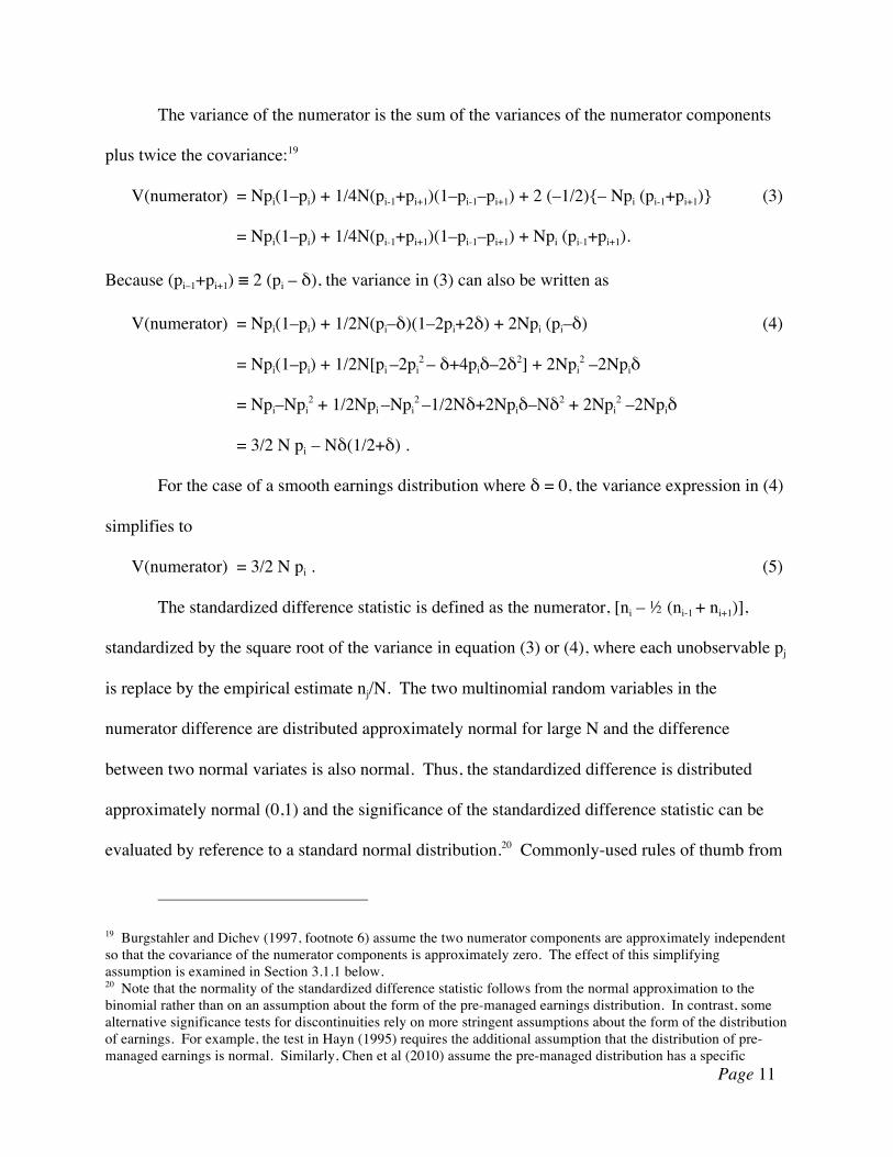
The variance of the numerator is the sum of the variances of the numerator components

plus twice the covariance:19

V(numerator) = Npi(1–pi) + 1/4N(pi-1+pi+1)(1–pi-1–pi+1) + 2 (–1/2){– Npi (pi-1+pi+1)} (3)

= Npi(1–pi) + 1/4N(pi-1+pi+1)(1–pi-1–pi+1) + Npi (pi-1+pi+1).

Because (pi–1+pi+1) ≡ 2 (pi – δ), the variance in (3) can also be written as

V(numerator) = Npi(1–pi) + 1/2N(pi–δ)(1–2pi+2δ) + 2Npi (pi–δ) (4)

= Npi(1–pi) + 1/2N[pi –2pi2

– δ+4piδ–2δ2] + 2Npi2 –2Npiδ

= Npi–Npi2 + 1/2Npi –Npi

2 –1/2Nδ+2Npiδ–Nδ2 + 2Npi

2 –2Npiδ

= 3/2 N pi – Nδ(1/2+δ) .

For the case of a smooth earnings distribution where δ = 0, the variance expression in (4)

simplifies to

V(numerator) = 3/2 N pi . (5)

The standardized difference statistic is defined as the numerator, [ni – ½ (ni-1 + ni+1)],

standardized by the square root of the variance in equation (3) or (4), where each unobservable pj

is replace by the empirical estimate nj/N. The two multinomial random variables in the

numerator difference are distributed approximately normal for large N and the difference

between two normal variates is also normal. Thus, the standardized difference is distributed

approximately normal (0,1) and the significance of the standardized difference statistic can be

evaluated by reference to a standard normal distribution.20 Commonly-used rules of thumb from

19 Burgstahler and Dichev (1997, footnote 6) assume the two numerator components are approximately independent so that the covariance of the numerator components is approximately zero. The effect of this simplifying assumption is examined in Section 3.1.1 below. 20 Note that the normality of the standardized difference statistic follows from the normal approximation to the binomial rather than on an assumption about the form of the pre-managed earnings distribution. In contrast, some alternative significance tests for discontinuities rely on more stringent assumptions about the form of the distribution of earnings. For example, the test in Hayn (1995) requires the additional assumption that the distribution of pre-managed earnings is normal. Similarly, Chen et al (2010) assume the pre-managed distribution has a specific

the statistics literature suggest that the normal approximation to the binomial is reasonably

accurate for Np(1-p) ≥ 25.21 In typical applications where p is small so that Np(1-p) ≅ Np, the

statistical rule of thumb is approximately equivalent to the condition that the expected interval

sample size, Npi , is 25 or larger.22 For sufficiently large expected values of Npi=E[ni] and N(pi–

1+pi+1)=E[ni–1+ni+1], the standardized difference statistic is distributed approximately normal. For

smaller interval sample sizes, the continuous normal approximation to the discrete multinomial

distribution may be more problematic, and we present simulation evidence on the behavior of the

standardized difference statistic for interval sample sizes much smaller than 25.

3.1 Relation to previous derivations in the literature

3.1.1 BD assumption of independence of the numerator components

BD invoke a simplifying assumption that the number of observations in interval i and the

sum of the numbers of observations in intervals i–1 and i+1 are independent. Therefore, the BD

variance expression omits the covariance term in (4), 2Npi (pi–δ). Omission of the covariance

term results in a misstatement relative to the correct variance in (4) of:

Relative Misstatement = –[2Npi (pi–δ)] / [3/2Npi –Nδ(1/2+δ)] .

distributional form. In both cases, a significant test statistic could be due to a discontinuity but could instead be due to departures from the assumed pre-managed earnings distribution. Other statistical tests assume the pre-managed distribution is known or can be estimated without error. For example, Bollen and Pool (2009) assume that the pre-managed distribution of hedge fund returns is perfectly described by a distribution fitted to the histogram of reported hedge fund returns, as they assume there is no variance in their test statistic attributable to the use of the fitted distribution as an estimate of the unmanaged hedge fund return distribution. Still other alternative tests rely on the assumption that variability of the test statistic for the test interval can be estimated based on variability of a similar statistic in non-test intervals. For example, Degeorge, Patel, and Zeckhauser (1999) test whether the increment in observations at the earnings benchmark is significant relative to the variance of increments in a symmetric set of 10 intervals surrounding the benchmark. 21 Although they are not considered here, corrections for small sample sizes, including a simple continuity correction (see Johnson and Kotz equations 33 and 36, p. 62-64) are available and could be used to improve evaluations of significance when Npi < 25. 22 When the interval sample size is 25 or larger, the error induced by using estimated probabilities in calculating the variance is likely to be small. However, when the standardized difference test is applied to much smaller interval sample sizes, the use of estimated probabilities can lead to more serious errors. For example, in the extreme case where a very low interval sample size gives rise to an empirical frequency of zero, the estimated variance based on the zero frequency is zero.

Because the expression –[2Npi (pi–δ)] is virtually always negative, the BD assumption generally

results in an understatement of the variance.23 Further, for the specific case of a smooth

distribution where δ=0, the understatement simplifies to

= –[2Npi2 ] / [3/2Npi ]

= –(4/3) pi

The understatement of the variance results in a corresponding (though slightly smaller)

percentage overstatement of the test statistics.24

3.1.2 BMN "correction"

BMN footnote 12 claims that the variance of the standardized difference test statistic

derived in BD and widely used in the literature is incorrect: "The correct variance, however, is

Npi(1-pi) + 1/4N(pi-1+pi+1)(2–pi-1–pi+1). Because of the difference in the first term in the last

parentheses, the estimated standard deviation used in BD and related papers is understated,

resulting in an overstatement of the standardized difference test statistic." However, BMN

provide neither a derivation for their "correction", nor an explanation of the purported error in

the BD derivation.

The BMN expression for variance is substantially larger than the variance in equation (4).

To see this, the BMN expression can be rewritten as the variance in equation (4) less the

covariance term (the term that is omitted in the BD simplification), 2Npi (pi–δ), plus a final

unexplained term, 1/4N(pi-1+pi+1):

VBMN = [Npi(1-pi) + 1/4N(pi-1+pi+1)(2-pi-1–pi+1) ] (6)

23 This expression is never positive but it can be equal to zero if pi=0 or if both pi-1 and pi+1 are equal to zero. 24 Since the standardized difference is standardized by the square root of the variance, a (4/3)pi relative understatement of the variance translates into understatement of the standard deviation by the square root of [1 - (4/3)pi] and a corresponding overstatement of the standardized difference statistic by the reciprocal of [1 - (4/3)pi]1/2. For example, when pi = .01, .03, or .05 and the distribution is smooth, the BD approximation overstates the test statistic by about .7%, 2.1%, or 3.5%, respectively.

= [Npi(1-pi) + 1/4N(pi-1+pi+1)(1-pi-1–pi+1) ] + [1/4N(pi-1+pi+1)]

= [Npi(1-pi)+1/4N(pi-1+pi+1)(1-pi-1–pi+1)] + [2Npi(pi–δ)] – [2Npi(pi–δ)] + [1/4N(pi-1+pi+1)]

= 3/2Npi – Nδ(1/2+δ) – [2Npi(pi–δ)] + [1/4N(pi-1+pi+1)]

The resulting misstatement relative to the correct variance in (4) is:

Relative Misstatement = {– [2Npi(pi–δ)] + [1/4N2(pi–δ)] } / [3/2Npi – Nδ(1/2+δ)] .

The BMN expression results in an overstatement of the variance by about 1/3. For example, for

the specific case of a smooth distribution where δ=0, the relative misstatement reduces to

Relative Misstatement = {– [2Npi2] + [1/4N2pi] } / [3/2Npi ]

= –(4/3)pi + [1/3 ] .

Because the variance is overstated by almost 1/3, standardized differences constructed using the

overstated variance have a standard deviation slightly less than the reciprocal of the square root

of 4/3 which is slightly greater than .866.

4. Simulation Evidence on the Distribution of the Standardized Difference Statistic

Table 1 reports the results of a simulation analysis that serves four purposes. First, in the

simulation the probabilities for each interval are known, and these known probabilities can be

used to compute the variance in equation (4) or (5). The means and variances of standardized

differences where the denominator variance is calculated using the known interval probabilities

are compared with the derived means and variances to verify the derivation. Second, the

simulation illustrates the behavior of the test statistic under conditions where the probabilities

that determine the denominator variance are estimated rather than known. Results are provided

for both large sample sizes, where the effect of using estimated probabilities should be minor,

and for smaller sample sizes where the effect may be more substantial. Third, the simulation

provides examples of the effect of 1) the use of estimated probabilities, and 2) departures from

the null hypothesis assumption of smoothness on tests of significance. While these examples are

based on the simulated normal earnings distribution, the examples illustrate how the effect of

departures from smoothness can be explored for any earnings distribution. Finally, the results

provide evidence on the behavior of the test statistic using the simplified variance approximation

from BD or using the incorrect expression suggested in BMN.

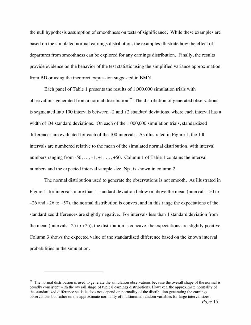
Each panel of Table 1 presents the results of 1,000,000 simulation trials with

observations generated from a normal distribution.25 The distribution of generated observations

is segmented into 100 intervals between –2 and +2 standard deviations, where each interval has a

width of .04 standard deviations. On each of the 1,000,000 simulation trials, standardized

differences are evaluated for each of the 100 intervals. As illustrated in Figure 1, the 100

intervals are numbered relative to the mean of the simulated normal distribution, with interval

numbers ranging from -50, …, -1, +1, …, +50. Column 1 of Table 1 contains the interval

numbers and the expected interval sample size, Npi, is shown in column 2.

The normal distribution used to generate the observations is not smooth. As illustrated in

Figure 1, for intervals more than 1 standard deviation below or above the mean (intervals –50 to

–26 and +26 to +50), the normal distribution is convex, and in this range the expectations of the

standardized differences are slightly negative. For intervals less than 1 standard deviation from

the mean (intervals –25 to +25), the distribution is concave, the expectations are slightly positive.

Column 3 shows the expected value of the standardized difference based on the known interval

probabilities in the simulation.

25 The normal distribution is used to generate the simulation observations because the overall shape of the normal is broadly consistent with the overall shape of typical earnings distributions. However, the approximate normality of the standardized difference statistic does not depend on normality of the distribution generating the earnings observations but rather on the approximate normality of multinomial random variables for large interval sizes.

Table 1 Panel A shows results for samples corresponding to 64,000 earnings

observations, corresponding to typical sample sizes encountered in earnings management

contexts.26 Panel B shows results for samples of 4,000 observations, illustrating the effects of a

far smaller sample size, where there will be more substantial divergence between the continuous

normal distribution that is used to approximate the discrete multinomial distribution.

4.1 Verification of distribution

In both Panels A and B, Columns 4 and 5 show the means and standard deviations when

the numerator of the generated standardized difference statistics is divided by the square root of

the variance computed using the known interval probabilities. These standardized difference test

statistics should have a mean equal to the theoretical expectation shown in column 3, and a

standard deviation equal to one. In both panels, the difference between the average empirical

mean in column 4 and the average theoretical mean in column 3 is less than .00001 and the

standard deviation of the differences between the empirical mean in column 4 and the theoretical

mean in column 3 is less than .001, the expected standard deviation for estimates of a random

variable with unit variance when the estimates are based on 1,000,000 simulation trials. Also,

the average of the standard deviations of the empirical standardized differences in column 5 is

1.00003 in Panel A and 1.0001 in Panel B, where the minimum of all the estimated standard

deviations is .99244 and the maximum is 1.00825. Thus, the results in columns 4 and 5 are

consistent with the distribution of the standardized difference derived in Section 3.

26 For example, BD examined distributions of earnings levels with a sample size of about 75,000 and distributions of earnings changes with a sample size of approximately 65,000.

4.2 Distribution using estimated variances

In any application of the standardized difference statistic, the computed variance of the

numerator must rely on estimated, rather than known, interval probabilities. Variances using

estimated interval probabilities are subject to greater estimation error for smaller expected

interval sample sizes (small N pi), so there can be more substantial differences between the

estimated and true variances.

Column 6 shows the average standardized differences when the variance is based on

estimated probabilities. The average difference between the standardized differences using

known versus estimated probabilities is less than .00001 and the standard deviation of the

differences using known versus estimated probabilities is less than .001 in both Panels A and B.

Column 7 shows the empirical standard deviation of the standardized difference statistics based

on estimated interval probabilities. In Panel A, where interval sample sizes are 16 times larger,

the mean standard deviation in Column 7 is 1.0036 and the range is .9947 to 1.0125. In Panel B,

the mean standard deviation in Column 7 is 1.0092 and the range is 1.0055 to 1.0182. Thus, the

use of estimated probabilities in applications appears to result in only a very small increase in the

standard deviation of the test statistic, with standard deviations that average about 1.004 for the

large interval sample sizes in Panel A and about 1.009 for the smaller interval sizes in Panel B.

The next section shows that these small increases in standard deviation lead to only small effects

on effective levels of significance.

4.3 Effects of departures from smoothness on significance tests

The null hypothesis of smoothness does not hold precisely for most plausible

distributions of pre-managed earnings. For example, the normal distribution used to generate

observations in the simulation is not smooth, but rather is concave within 1 standard deviation of

the mean and convex beyond 1 standard deviation. Thus, the results of the simulation illustrate

the effect of departures from smoothness for one example, the normal distribution. Perhaps more

importantly, the analysis illustrates how to assess the effect of departures from smoothness for

any other specified distribution.

The expectations shown in column 3 reflect the effect of departure from smoothness on

the standardized difference statistic. As the expectations become more positive, the proportion

of significant test statistics should begin to exceed 5%. Conversely, as expectations become

more negative, the proportion should be less than 5%.27 The proportions of significant test

statistic in column 10 are highly consistent with proportions predicted based on the expectation

for each interval.28 For the normal distribution and interval definitions in the simulation,

departures from the nominal 5% level are minimal – the maximum predicted proportion

significant is 5.22% (for simulation intervals –1 and +1) and the maximum proportion significant

realized in the simulation is 5.30% (for interval +2).

The width of the interval and the location of the distribution relative to the benchmark are

important determinants of the effect of departures from smoothness. The simulation results

suggest that the departures from smoothness for a normal generating distribution have little

practical effect on significance tests for interval widths of about .04. However, the effect can be

much larger for much wider intervals. For example, with the same normal generating

distribution, interval widths of .5 standard deviation, and the distribution located such that the

27 For example, when the expected standardized difference is .021, the expected rejection rate for a one-tailed test is .0522, the probability of observing a value greater than 1.645 for a normal variate with mean .021 and standard deviation of 1. Thus, the expected rejection rate is about 5.2% in intervals -3 to +3 in Panel A. Similarly, when the expected standardized difference is –.022, the expected rejection rate is .0478, the probability of a value greater than 1.645 for a normal variate with mean –.022 and standard deviation of 1. Thus, the expected rejection rate is about 4.8% in intervals -49 to –47 or +47 to +49 in Panel A. 28 The average difference (not reported in the table) between the realized proportion significant and the predicted rate is –.0014 in Panel A and –.0007 in Panel B and the standard deviation of the difference between the realized proportion significant and the predicted rate is .0011 in Panel A and .0025 in Panel B.

benchmark falls at the mean of the distribution, the expected standardized differences for

intervals –1 and +1 are each positive with identical expectations of 10.00 (2.50) for N = 64,000

(4,000). Thus, using intervals equal to .5 standard deviations (far wider than is typically used in

tests for earnings management) would lead to a rejection rate of essentially 100% for N=64,000

when there is no earnings management. As another example, with interval widths of .5 standard

deviation and the distribution located such that the benchmark falls .25 standard deviations

below the mean of the distribution so that interval +1 is centered at the peak of the distribution,

the expectation is 10.79 (2.70) for N = 64,000 (4,000).

4.4 Effects of BD and BMN variances

Column 8 shows the empirical standard deviation of the standardized difference statistics

generated for each interval when the denominator variance is calculated using the BD

independence assumption. Consistent with the analysis in section 3, the BD independence

assumption yields a test statistic with a standard deviation roughly 1% greater than the

theoretical standard deviation of 1. The average standard deviation in column 8 is 1.007 in Panel

A and 1.012 in Panel B. This small inflation of the standard deviation of the standardized

difference statistic leads to a small corresponding inflation of the proportion of significant test

statistics. In column 11, the additional proportion significant using the BD independence

assumption ranges from .01% to almost .1%, with an average of .055%. Thus, under the

simulation conditions, the effect of using the BD independence assumption in tests of the

significance of the standardized differences is very small.

Column 9 shows the empirical standard deviation of the standardized difference statistics

when the standard deviation of the statistic is calculated using the BMN expression for variance.

Consistent with the analysis in section 3, the average standard deviations in column 9 are slightly

greater than .866, specifically .8702 in Panel A and .8709 in Panel B. Column 11 shows that

using the BMN expression yields an effective level of about 3% for a test with a nominal level of

5%. The proportion of significant test statistics ranges from 1.11% to 2.15% below the 5% level,

with an average of 1.98% in Panel A and 1.60% in Panel B. This lower effective level will result

in substantially lower power of tests using the BMN expression.

4.5 Summary

In summary, the simulation results in Table 1 are consistent with the analysis in Section

3. When the variance of the numerator of the standardized difference statistic is computed using

the interval probabilities that are known in the simulation, the empirical distribution of the

standardized difference statistic is consistent with the theoretical distribution derived in Section

3. When the variance is computed using estimated, rather than known, interval probabilities the

distribution continues to be consistent with the standard normal distribution for intervals with an

expected sample size greater than 25. Even for the interval sample sizes in Panel B less than 25

where the normal approximation is more problematic, departures from the assumed standard

normal remain relatively minor. Finally, standardized differences relying on the simplifying BD

independence assumption to compute the denominator variance have standard deviations about

1% larger than standardized differences using the correct variance expression, resulting in

rejection rates no more than a fraction of one percent higher than rates using the correct variance

expression.

5. Power of the Standardized Difference Test for Discontinuities

Earnings management to meet a benchmark transforms pre-managed observations in

intervals below the benchmark into reported (post-managed) earnings above the benchmark.

When the unobservable distribution of pre-managed observations is smooth, earnings

management creates a trough below the benchmark and a peak above the benchmark in the post-

managed distribution. Standardized difference statistics are designed to be sensitive to

departures from smoothness due to earnings management.

The power of standardized difference tests to detect earnings management is determined

by 1) the pre-managed earnings distribution in the vicinity of the benchmark, and 2) the specific

way that earnings are managed.

5.1 Pre-managed earnings distribution

The power of tests for a discontinuity at the benchmark depends on the probabilities that

a pre-managed earnings observation will fall in the two intervals immediately below the

benchmark, referred to here as intervals –2 and –1, and in the two intervals immediately above

the benchmark, referred to here as intervals +1 and +2.29 These probabilities depend on where

the benchmark falls relative to the distribution, i.e., how far the benchmark is in the tail of the

distribution, and which side of the distribution the benchmark is on.

Tests for management with respect to benchmarks further in the tail will have lower

power because there are fewer pre-managed observations below the benchmark to be managed.

Power is determined by a combination of the total number of observations in the earnings

distribution, N, and the probability of pre-managed observations in the interval(s) below the

benchmark that could be managed to meet the benchmark. In the following analysis,, we

consider the specific case where only observations in the interval immediately below the

benchmark are managed to meet the benchmark, so power is determined by N and the probability

of pre-managed earnings observations in the interval immediately below the benchmark, referred

29 Note that in section 4 where we were considering the null hypothesis, intervals were numbered relative to the mean of the distribution, where –1 and +1 were the intervals immediately below and above the mean. In this section, intervals are numbered relative to the benchmark, where –1 and +1 are the intervals immediately below and above the benchmark.

to as the interval sample size for interval –1. Denoting the cumulative probability that a pre-

managed earnings observation falls in interval –1 as p-1, the interval sample size for interval –1 is

n–1 = Np–1.30 In the example power calculations below, p–1 is set at .01 and power is evaluated

for N ranging from 1,000 to 128,000, so the interval sample sizes range from 10 to 1,280.

Results in the N=1,000 and N=2,000 columns where interval sample sizes are 10 and 20,

respectively, should be interpreted cautiously in light of evidence from the statistics literature

that the normal provides a reasonable approximation to the multinomial for expected sample

sizes of 25 or greater.

Power also depends on which side of the distribution the benchmark falls. For example,

when the benchmark falls below the mode of a typical symmetric earnings distribution, p-2<p-

1<p+1<p+2. On the other hand, when the benchmark falls above the mode, the inequalities are all

reversed. Power will also depend on the relative values for probabilities in adjacent intervals

(e.g., how much larger is p+2 than p+1, or how much larger is p+1 than p–1) which in turn depends

on the specific earnings distribution and on the location of the benchmark relative to the

distribution. Because the inequalities relating the probabilities in the four intervals could go

either direction and because there is no general relationship among the relative values of the

probabilities, we adopt the simplifying assumption that the pre-managed probabilities are all

equal to the probability for interval –1, so that p-2 = p-1 = p+1 = p+2 = .01.

30 The location of the benchmark relative to the peak of the pre-managed earnings distribution can also affect the interpretation of the standardized difference test. This issue is relatively unimportant for well-behaved theoretical earnings distributions such as the normal distribution used in the simulation. (See the results in Table 1 for the intervals immediately adjacent to 0.) However, because empirical distributions often are far more leptokurtic than the normal distribution, sometimes modeled as mixtures of normal distributions or as symmetric stable distributions, empirical evidence of a significant standardized difference at the peak of the distribution should generally not be interpreted as evidence of earnings management.

5.2 Assumptions about how earnings are managed

The power of the standardized difference test also depends on how earnings are managed.

In this section, we illustrate power calculations for one assumption. To the extent this

assumption is a reasonable representation of how earnings are managed, these calculations are

interesting in their own right. However, the calculations also serve to illustrate how power can

be calculated for any assumption about how earnings are managed. We consider the specific

assumption that earnings management effects are concentrated entirely in the interval

immediately below and the interval immediately above the benchmark, i.e., earnings in interval

–1 are managed upward so that reported (post-managed) earnings is in interval +1.

5.2.1 Rate of earnings management (r)

We assume the probability of earnings management is r, representing the rate of earnings

management.31 Because earnings are managed from interval – to interval +1, the expected

number of reported earnings observations in interval –1 is less than the average of the numbers

of observations in the adjacent intervals, i.e., intervals –2 and +1. Thus, the left standardized

difference, the standardized difference for the first interval left of the benchmark has a negative

expectation. Similarly, the expected number of observations in interval +1 is greater than the

average of the adjacent intervals, i.e., intervals –1 and +2 and therefore the expectation of the

right standardized difference, the standardized difference for the first interval above the

benchmark, is positive.32 Other patterns of earnings management can be described in terms of

more complex concentration effects, considered next.

31 For example, BD estimate that the rate of earnings management among firms with small pre-managed losses is in the range of 30-44% and the rate among firms with small pre-managed earnings decreases is 8-12%. 32 For this simple form of earnings management, the left and right standardized difference are alternative, but highly-correlated, tests for the effect of earnings management. For more complex forms of earnings management, either the left or right standardized differences may provide a more appropriate test, as discussed in more detail later.

5.2.2 Concentration

Concentration is determined by both how earnings are managed and by the choice of

interval width in the research design. The results below analyze the research design choice of

interval width, holding constant the assumption about how earnings are managemed.

Specifically, we consider the effect on power 1) when interval width is cut in half so that

earnings are being managed from two intervals below the benchmark and managed to two

intervals above the benchmark, and 2) when interval width is doubled so that the first interval

below the benchmark includes both the original set of observations where earnings are being

managed and a second set of observations where earnings are not being managed.

More complex models might describe which pre-managed earnings observations are

subject to earnings management, and how the post-managed earnings observations are

distributed. For example, observations might be managed from more than one interval below the

benchmark, rather than only the single interval immediately below the benchmark, where the rate

of management likely decline for intervals further below the benchmark. Further, earnings might

be managed to more than one interval above the benchmark. Evaluation of these possibilities is

left for future research.

5.3 Analysis of the Power of the standardized difference test

The mean and variance of the standardized difference statistic given in equations (2) and

(4), respectively, can be used to compute power under any specified alternative hypothesis.

Power, denoted by 1–β, is a function of the level of the test, denoted by α.33 An observed

33 The logic for rejection of the null when a significant statistic is observed is that a significant statistic is more likely to occur under the alternative (with probability 1-β) than under the null (with probability α). Thus, the strength of the evidence that a significant result provides in favor of the alternative is described by the ratio (1–β)/α. As the ratio approaches one (i.e., as power falls close to the level of the test), the effect of a significant test statistic on belief in null versus the alternative disappears. For further discussion, see, for example, Burgstahler (1987).

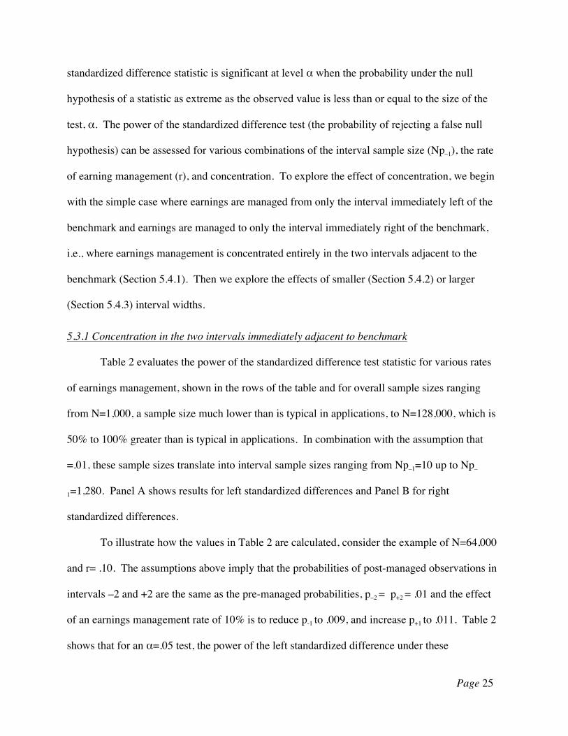
standardized difference statistic is significant at level α when the probability under the null

hypothesis of a statistic as extreme as the observed value is less than or equal to the size of the

test, α. The power of the standardized difference test (the probability of rejecting a false null

hypothesis) can be assessed for various combinations of the interval sample size (Np–1), the rate

of earning management (r), and concentration. To explore the effect of concentration, we begin

with the simple case where earnings are managed from only the interval immediately left of the

benchmark and earnings are managed to only the interval immediately right of the benchmark,

i.e., where earnings management is concentrated entirely in the two intervals adjacent to the

benchmark (Section 5.4.1). Then we explore the effects of smaller (Section 5.4.2) or larger

(Section 5.4.3) interval widths.

5.3.1 Concentration in the two intervals immediately adjacent to benchmark

Table 2 evaluates the power of the standardized difference test statistic for various rates

of earnings management, shown in the rows of the table and for overall sample sizes ranging

from N=1,000, a sample size much lower than is typical in applications, to N=128,000, which is

50% to 100% greater than is typical in applications. In combination with the assumption that

=.01, these sample sizes translate into interval sample sizes ranging from Np–1=10 up to Np–

1=1,280. Panel A shows results for left standardized differences and Panel B for right

standardized differences.

To illustrate how the values in Table 2 are calculated, consider the example of N=64,000

and r= .10. The assumptions above imply that the probabilities of post-managed observations in

intervals –2 and +2 are the same as the pre-managed probabilities, p–2 = p+2 = .01 and the effect

of an earnings management rate of 10% is to reduce p-1 to .009, and increase p+1 to .011. Table 2

shows that for an α=.05 test, the power of the left standardized difference under these

assumptions is .938 and the power of the right standardized difference is .916.34 The

assumptions in this example correspond to an expectation of 640 pre-managed observations in

the interval left of the benchmark, with just 640 x .1 = 64 observations expected to be managed

to exceed the benchmark. Thus, the results show that standardized difference tests have power in

excess of 90% to detect management for just 64 observations in a distribution of 64,000, or just

.1% of the total number of observations.

As another example, for N=16,000, an earnings management rate of just .20 yields power

in excess of 90%. Thus, .20 x 160 = 32 observations out of 16,000 observations managed to

exceed the benchmark or just .2% are sufficient for the standardized difference tests to have

power greater than 90%. As a final example, Panel A shows that the left standardized difference

is expected to be significant more than 90% of the time when just 8,000 x .01 x .300 = 24

observations are managed to meet the benchmark in a sample of 8,000 observations.

The shading in Panels A and B demarcates different strata of power. Cells where power

is 1.000 are shaded dark gray,35 cells with power greater than .900 are medium gray, and cells

with power greater than .500 are light gray. Overall, the results show that when the effects of

earnings management are concentrated entirely in the interval below and above the benchmark

and when the intervals in the vicinity of the benchmark contain about 1% of the distribution, the

standardized difference tests have power greater than .900 to detect small rates and small

numbers of observations managed to meet the benchmark.

34 These values are computed by using equations (2) and (4) to compute the mean and standard deviation, respectively, of the left-standardized difference given the values p-2 , p-1 , and p+1 and of the right-standardized difference given the values p-1 , p+1 , and p+2. Then, the mean and standard deviation of each standardized difference distribution are used to find the probability of a left-standardized difference less than the critical value of –1.64485 and the probability of a right-standardized difference greater than 1.64485. 35 More precisely, the power in these cells is greater than .9995, so the values round to 1.000 with three decimal places of accuracy.

Of course, in applications it is unlikely that interval widths can be identified such that the

effects of earnings management are concentrated entirely in the interval below and above the

benchmark. Instead, it is likely that the rate of earnings management declines for observations

further below the benchmark and that probability that an observation will be managed to exceed

the benchmark by a given amount will decline with the magnitude of the amount. Thus, interval

width is a difficult and important choice in designing tests of earnings management. While it is

not possible to delineate and evaluate all the possible effects of interval width choice for all

possible types of earnings management behavior, we provide results below showing the effect of

choosing an interval width that is too narrow or too wide relative to the case illustrated in Table

2, where earnings management behavior is such that all effects are concentrated in the interval

immediately below and above the benchmark. That is, we maintain the assumptions that

earnings are managed from an interval below the benchmark with pre-managed probability =.01

at some rate r that applies uniformly to the entire interval, and that the managed observations are

distributed uniformly in an interval above the benchmark with pre-managed probability =.01. In

Section 5.4.2, we evaluate the effect on power of using a research design with an interval width

that is only half as wide as the intervals in which earnings are concentrated (so that the

implemented intervals widths have pre-managed probabilities = .005). In Section 5.4.3, we

evaluate the effect on power of using a research design with an interval width that is twice as

wide as the intervals in which earnings are concentrated (so that the implemented intervals

widths have pre-managed probabilities = .02).

5.3.2 Intervals half as wide as the .01 interval in which earnings management is concentrated

Table 3 shows the power of the standardized difference test statistic when the pre-

managed interval width is .005 and the effects of earnings management are concentrated in two

intervals below the benchmark and in two intervals above the benchmark. The rates in the rows

of the table represent the rate of earnings management among pre-managed earnings

observations in the first two intervals below the benchmark, interval –2 and –1, where the

cumulative probability of pre-managed observations in these two interval p–2 + p–1, is assumed to

be .01. Managed observations are assumed to move to the first two intervals above the

benchmark, intervals +1 and +2. Panel A shows results for left standardized differences and

Panel B for right standardized differences.

Because the effects of earnings management are now spread across multiple intervals, the

prominence of the trough and peak relative to the surrounding intervals are reduced, and the

power of the standardized difference tests is also reduced. Focusing on the same example we

considered in Section 5.4.1 where N=64,000 and r= .10, the assumptions imply that the

probabilities of post-managed observations in the four intervals are p-2 = p-1 = .0045, and p+1 = p+2

= .0055. In words, earnings management is expected to transform 10% of the pre-managed

observations in intervals –2 and –1 into post-managed observations in intervals +1 and +2, so

that the probabilities of a post-managed observation in intervals –2 and –1 are .0045 (so the total

probability is .009, the same as in interval –1 in Section 5.4.1) and the probabilities of a post-

managed observation in interval +1 or +2 are .0055 (so the total probability in the two intervals

is .011, the same as in interval +1 in Section 5.4.1). Table 3 shows that for an α=.05 test, the

power of the left standardized difference under these assumptions is .447 and the power of the

right standardized difference is .409, computed by using equations (2) and (4) to compute the

mean and standard deviation and finding the probability of a left-standardized difference less

than –1.64485 and the probability of a right-standardized difference greater than 1.64485. Thus,

using interval width that is much narrower than the interval width in which earnings management

is concentrated results in a substantial loss of power for this example.

Panels C and D facilitate the comparison of the power results in Table 3 with the

corresponding amounts in Table 2, and shows that the use of a too narrow interval width can

result in a substantial loss of power. Panels C and D show gray shading for the cells where there

cannot be much loss of power when the interval width is too narrow, either because the power is

very high even with the narrow interval width in Table 3 (the dark gray shading corresponds to

cells where the power in Panels A and B exceeds .900) or because the power is very low even

with the optimal interval width in Table 2 (the light gray shading corresponds to cells where the

power in Table 2 is less than .100). The remaining, unshaded cells in Table 3 Panels C and D

show that the power using the too narrow interval width assumed in Table 3 is often on the order

of 40%-60% of the power using the optimal interval width in Table 2. Thus, too narrow

intervals can substantially reduce the power of standardized difference tests.

5.3.3 Intervals twice as wide as the .01 interval in which earnings management is concentrated

Table 4 shows the power of the standardized difference test statistic when the pre-

managed interval width is .02 so that observations affected by earnings management are

combined with observations not affected by earnings management in the interval below the

benchmark and the interval above the benchmark. The rates in the rows of the table represent

twice the rate of earnings management among pre-managed earnings observations in the interval

below the benchmark where the cumulative probability of pre-managed observations in the

interval, p–1, is now assumed to be .02. Managed observations are assumed to move to the first

interval above the benchmark, intervals +1. Panel A shows results for left standardized

differences and Panel B for right standardized differences.

Because intervals affected by earnings management are now combined with intervals not

affected by earnings management, the power of the standardized difference tests is again

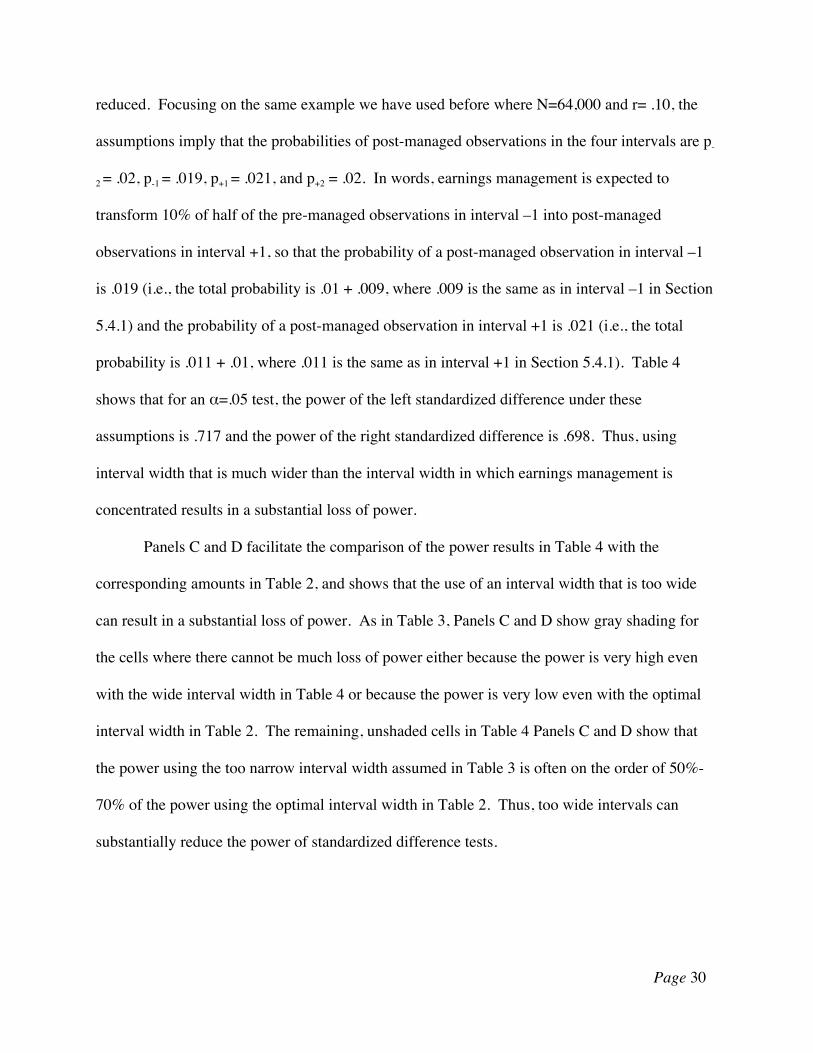
reduced. Focusing on the same example we have used before where N=64,000 and r= .10, the

assumptions imply that the probabilities of post-managed observations in the four intervals are p-

2 = .02, p-1 = .019, p+1 = .021, and p+2 = .02. In words, earnings management is expected to

transform 10% of half of the pre-managed observations in interval –1 into post-managed

observations in interval +1, so that the probability of a post-managed observation in interval –1

is .019 (i.e., the total probability is .01 + .009, where .009 is the same as in interval –1 in Section

5.4.1) and the probability of a post-managed observation in interval +1 is .021 (i.e., the total

probability is .011 + .01, where .011 is the same as in interval +1 in Section 5.4.1). Table 4

shows that for an α=.05 test, the power of the left standardized difference under these

assumptions is .717 and the power of the right standardized difference is .698. Thus, using

interval width that is much wider than the interval width in which earnings management is

concentrated results in a substantial loss of power.

Panels C and D facilitate the comparison of the power results in Table 4 with the

corresponding amounts in Table 2, and shows that the use of an interval width that is too wide

can result in a substantial loss of power. As in Table 3, Panels C and D show gray shading for

the cells where there cannot be much loss of power either because the power is very high even

with the wide interval width in Table 4 or because the power is very low even with the optimal

interval width in Table 2. The remaining, unshaded cells in Table 4 Panels C and D show that

the power using the too narrow interval width assumed in Table 3 is often on the order of 50%-

70% of the power using the optimal interval width in Table 2. Thus, too wide intervals can

substantially reduce the power of standardized difference tests.

6. Conclusion

A large body of literature documents discontinuities in earnings distributions at

prominent earnings benchmarks. These discontinuities have been widely interpreted as

consistent with the theory that managers take actions to ensure that earnings meet benchmarks.

This interpretation is supported by survey evidence in Graham, Harvey, and Rajgopal (2005)

indicating that managers are willing to incur real costs in order to meet such benchmarks.

However, in situations where both discontinuity evidence and accruals-based models have been

applied, abnormal accruals models have failed to find evidence that earnings management using

accruals explain discontinuities.

This paper reviews and refines the derivation of the distribution of the Burgstahler and

Dichev (1997) standardized difference statistic and corrects an error introduced into the literature

in Beaver, McNichols, and Nelson (2007). The paper also provides a formal evaluation of the

statistical properties of discontinuity tests to detect earnings management. The analysis shows

the importance of defining interval widths that result in concentration of the effects of earnings

management in the interval immediately below and the interval immediately above the

benchmark – much narrower or much wider interval widths can substantially reduce the power of

standardized difference tests.

The results show that standardized difference tests have the power to detect management

of relatively small amounts of earnings (say .25%–.50% of MVE) by a small proportion of firms

(say .1%–.2%). In contrast, previous research suggests that accruals-based tests have reasonable

power only for far larger amounts of earnings management by a much larger proportion of

sample firms (say 5% or more of total assets for all sample firms). Thus, together with evidence

from previous papers, the evidence suggests that discontinuity tests have far greater power to

detect smaller amounts and lesser rates of earnings management than do tests based on abnormal

accruals.

References

Ayers, B., J. Jiang, and P.E. Yeung. "Discretionary accruals and earnings management: An analysis of pseudo earnings targets." The Accounting Review 81 (October 2006): 617-652.

Ball, R. “Accounting Informats Investors and Earnings Management is Rife: Two Questionable Beliefts.” Unpublished Working Paper, University of Chcago, SSRN abstract=2211288 (2013).

Beaver, W., M. McNichols, and K. Nelson. “An Alternative Interpretation of the Discontinuity in Earnings Distributions,” Review of Accounting Studies (2007), Vol. 12, No. 4, 525-556.

Bollen, N., and V. Pool. Do hedge fund managers misreport returns? Evidence from the pooled distribution. The Journal of Finance 64:5 (2009), 2257-2288.

Brown, L. "A temporal analysis of earnings surprises: Profits versus losses," Journal of Accounting Research 39 (2001): 221–42.

Brown, L.D., and M.L. Caylor. "A Temporal Analysis of Quarterly Earnings Thresholds: Propensities and Valuation Consequences. The Accounting Review 80 (April 2005): 423-440.

Burgstahler, D. "Inference from Empirical Research." The Accounting Review, Vol. 62, No. 1 (January 1987): 203-214.

Burgstahler, D., and E. Chuk. “What Have We Learned About Earnings Management? Correcting Disinformation About Discontinuities.” Unpublished Working Paper, University of Washington (2013).

Burgstahler, D., and I. Dichev. “Earnings Management to Avoid Earnings Decreases and Losses.” Journal of Accounting & Economics 24 (1997): 99–126.

Burgstahler, D., and M. Eames. "Management of Earnings and Analysts’ Forecasts to Achieve Zero and Small Positive Earnings Surprise." Journal of Business Finance and Accounting. Vol. 33, No.5-6, (June/July 2006): 633-652.

Carslaw, C. “Anomalies in Income Numbers: Evidence of Goal Oriented Behavior.” The Ac- counting Review 63 (1988): 321–7.

Collins, D., and P. Hribar. , 2002. Errors in estimating accruals: implications for empirical research. Journal of Accounting Research 40, 105–135.

Das, S., and H. Zhang. "Rounding-up in reported EPS, behavioral thresholds, and earnings management." Journal of Accounting and Economics 35 (2003), 31-50.

Daske, H., G. Gebhardt, and S. McLeay. "The distribution of earnings relative to targets in the European Union." Accounting and Business Research 36:3 (2006), 137-167.

Dechow, P., A. Hutton, J. Kim, and R. Sloan. “Detecting Earnings Management: A New Approach.” Unpublished working paper, University of California, Berkeley, October 11, 2010.

Dechow, P., S. Richardson, and I. Tuna. “Why Are Earnings Kinky? An Examination of the Earnings Management Explanation,” Review of Accounting Studies (2003), Vol. 8, 355-384.

Dechow, P., R. Sloan and A. Sweeney, 1995, Detecting earnings management, The Accounting Review 70; 2: 193-225.

Degeorge, F., Patel, J., Zeckhauser, R. "Earnings manipulations to exceed thresholds." Journal of Business 72 (1999): 1–33.

Dichev, I., Skinner, D., 2002. Large sample evidence on the debt covenant hypothesis. Journal of Accounting Research 40, 1091–1123.

Donelson, D., McInnis, J., & Mergenthaler, R. "Discontinuities and earnings management: Evidence from restatements related to securities litigation." Contemporary Accounting Research 30:1 (2013): 242-268.

Durtschi, C., and P. Easton. “Earnings Management? The Shapes of the Frequency Distributions of Earnings Metrics Are Not Evidence ipso facto.” Journal of Accounting Research 43 (2005): 557–92.

Durtschi, C., and P. Easton. “Earnings Management? Erroneous Inferences Based on Earnings Frequency Distributions.” Journal of Accounting Research 47 (2009): 1249–1281.

Dyreng, S., Mayew, W., Schipper, K., 2012. Evidence that managers intervene in financial reporting to avoid working capital deficits. Working paper.

Ecker, F., J. Francis, P. Olsson, and K. Schipper. “Peer Firm Selection for Discretionary Accruals Models.” Unpublished working paper, Duke University, March 2011.

Graham, J., C. Harvey and S. Rajgopal. "The Economic Implications of Corporate Financial Reporting", Journal of Accounting and Economics 40 (2005): 3-73.

Grundfest, J. and N. Malenko. "Quadrophobia: Strategic Rounding of EPS Data." Stanford University Working paper, October 14, 2009.

Hayn, C., "The information content of losses." Journal of Accounting and Economics 20 [2] (1995): 125-153.

Healy, P., and J. Whalen. “A Review of the Earnings Management Literature and Its Implications for Standard Setting.” Accounting Horizons 13 (1999): 365–383.

Jensen, M. "Corporate Budgeting is Broken--Let’s Fix It." Harvard Business Review (November 2001).

Jensen, M. "Paying People to Lie: the Truth about the Budgeting Process." European Financial Management, Vol. 9, No. 3, 2003.

Johnson and Kotz (1969) Discrete Distributions, John Wiley & Sons : New York.

Kerstein, J., and A. Rai. "Intra-year shifts in the earnings distribution and their implications for earnings management"Journal of Accounting & Economics, Vol. 44 (2007): 399–419.

Kothari, S.P., A. Leone, and C. Wasley, 2005, Performance matched discretionary accruals measures, Journal of Accounting and Economics 39: 163-197.

Matsumoto, D. "Management's Incentives to Avoid Negative Earnings Surprises." The Accounting Review, Vol. 77, No. 3 (July 2002), pp. 483-514.

McNichols, M. "Research design issues in earnings management studies," Journal of Accounting and Public Policy 19 (2000), pp. 313–45.

Owens, E., J.S.Wu, and J. Zimmerman. “Business Model Shocks and Abnormal Accrual Models,” University of Rochester working paper, December 9, 2013.

Schipper, K. “Commentary on Earnings Management.” Accounting Horizons 3 (1989): 91–102.

Stubben, S. "Discretionary Revenues as a Measure of Earnings Management." The Accounting Review, Vol. 85, No. 2 (March 2010), pp. 695-717.

Thomas, J. "Unusual patterns in reported earnings." Accounting Review Vol. 64 No. 4 (1989): 773-787.

50 -26 -25 -1 +1 +25 +26 +50

Figure 1Intervals in Simulation

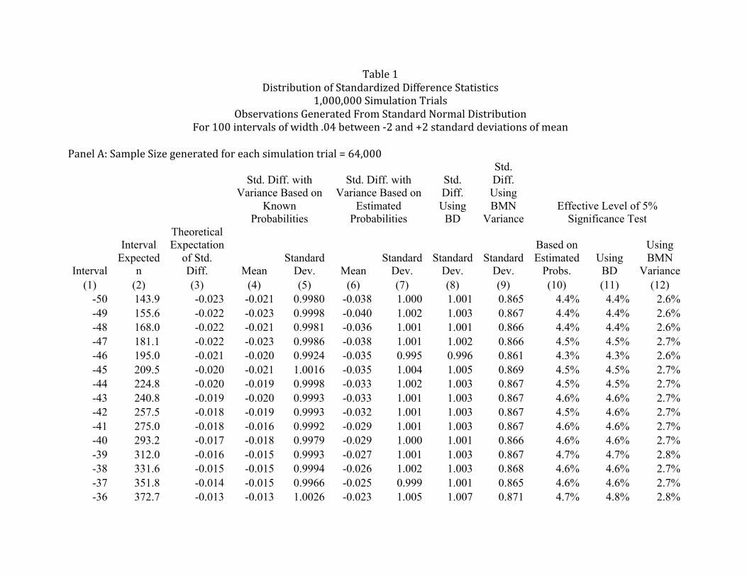
Table 1 Distribution of Standardized Difference Statistics

1,000,000 Simulation Trials Observations Generated From Standard Normal Distribution

For 100 intervals of width .04 between -‐2 and +2 standard deviations of mean Panel A: Sample Size generated for each simulation trial = 64,000

Std. Diff. with Variance Based on

Known Probabilities


Estimated Probabilities

Std. Diff. Using BD

Std. Diff. Using BMN

Variance Effective Level of 5%

Significance Test

Interval

Interval Expected

n

Theoretical Expectation

of Std. Diff. Mean

Standard Dev. Mean

Standard Dev.

Standard Dev.

Standard Dev.

Based on Estimated

Probs. Using BD

Using BMN

Variance (1) (2) (3) (4) (5) (6) (7) (8) (9) (10) (11) (12)

-50 143.9 -0.023 -0.021 0.9980 -0.038 1.000 1.001 0.865 4.4% 4.4% 2.6% -49 155.6 -0.022 -0.023 0.9998 -0.040 1.002 1.003 0.867 4.4% 4.4% 2.6% -48 168.0 -0.022 -0.021 0.9981 -0.036 1.001 1.001 0.866 4.4% 4.4% 2.6% -47 181.1 -0.022 -0.023 0.9986 -0.038 1.001 1.002 0.866 4.5% 4.5% 2.7% -46 195.0 -0.021 -0.020 0.9924 -0.035 0.995 0.996 0.861 4.3% 4.3% 2.6% -45 209.5 -0.020 -0.021 1.0016 -0.035 1.004 1.005 0.869 4.5% 4.5% 2.7% -44 224.8 -0.020 -0.019 0.9998 -0.033 1.002 1.003 0.867 4.5% 4.5% 2.7% -43 240.8 -0.019 -0.020 0.9993 -0.033 1.001 1.003 0.867 4.6% 4.6% 2.7% -42 257.5 -0.018 -0.019 0.9993 -0.032 1.001 1.003 0.867 4.5% 4.6% 2.7% -41 275.0 -0.018 -0.016 0.9992 -0.029 1.001 1.003 0.867 4.6% 4.6% 2.7% -40 293.2 -0.017 -0.018 0.9979 -0.029 1.000 1.001 0.866 4.6% 4.6% 2.7% -39 312.0 -0.016 -0.015 0.9993 -0.027 1.001 1.003 0.867 4.7% 4.7% 2.8% -38 331.6 -0.015 -0.015 0.9994 -0.026 1.002 1.003 0.868 4.6% 4.6% 2.7% -37 351.8 -0.014 -0.015 0.9966 -0.025 0.999 1.001 0.865 4.6% 4.6% 2.7% -36 372.7 -0.013 -0.013 1.0026 -0.023 1.005 1.007 0.871 4.7% 4.8% 2.8%

-35 394.1 -0.012 -0.010 1.0046 -0.021 1.007 1.009 0.873 4.8% 4.8% 2.9% -34 416.2 -0.011 -0.012 0.9996 -0.022 1.002 1.005 0.869 4.7% 4.7% 2.8% -33 438.7 -0.009 -0.009 1.0050 -0.019 1.008 1.010 0.873 4.9% 4.9% 2.9% -32 461.8 -0.008 -0.008 1.0036 -0.018 1.006 1.009 0.872 4.8% 4.9% 2.8% -31 485.2 -0.007 -0.007 0.9991 -0.016 1.002 1.005 0.869 4.7% 4.8% 2.8% -30 509.1 -0.006 -0.007 0.9998 -0.016 1.003 1.005 0.869 4.8% 4.8% 2.8% -29 533.3 -0.005 -0.003 1.0007 -0.012 1.004 1.007 0.870 4.8% 4.9% 2.8% -28 557.7 -0.003 -0.004 1.0036 -0.013 1.007 1.010 0.873 4.9% 5.0% 3.0% -27 582.3 -0.002 -0.002 1.0045 -0.010 1.008 1.011 0.874 5.0% 5.0% 3.0% -26 607.1 -0.001 -0.002 1.0034 -0.010 1.007 1.010 0.873 5.0% 5.0% 3.0% -25 631.8 0.001 0.002 0.9998 -0.006 1.003 1.007 0.870 4.9% 5.0% 2.9% -24 656.6 0.002 0.001 0.9975 -0.007 1.001 1.004 0.868 4.9% 4.9% 2.9% -23 681.2 0.003 0.005 0.9963 -0.003 1.000 1.004 0.867 4.9% 5.0% 2.9% -22 705.6 0.005 0.003 0.9980 -0.005 1.002 1.006 0.869 4.9% 5.0% 2.9% -21 729.7 0.006 0.006 0.9984 -0.002 1.003 1.006 0.870 4.9% 5.0% 2.9% -20 753.4 0.007 0.008 0.9965 0.000 1.001 1.005 0.868 4.9% 5.0% 2.9% -19 776.7 0.008 0.008 1.0000 0.000 1.004 1.008 0.871 5.0% 5.1% 3.0% -18 799.3 0.009 0.010 0.9996 0.003 1.004 1.008 0.871 5.0% 5.1% 3.0% -17 821.4 0.011 0.010 1.0026 0.002 1.007 1.011 0.874 5.1% 5.1% 3.0% -16 842.7 0.012 0.014 1.0048 0.007 1.009 1.014 0.876 5.2% 5.3% 3.1% -15 863.1 0.013 0.010 1.0043 0.003 1.009 1.014 0.876 5.1% 5.2% 3.1% -14 882.7 0.014 0.016 1.0077 0.009 1.012 1.017 0.879 5.2% 5.2% 3.1% -13 901.2 0.015 0.013 1.0063 0.006 1.011 1.016 0.878 5.2% 5.3% 3.1% -12 918.7 0.016 0.017 0.9947 0.010 1.000 1.004 0.868 5.0% 5.1% 3.0% -11 935.0 0.016 0.015 0.9954 0.008 1.000 1.005 0.868 5.0% 5.1% 3.0% -10 950.1 0.017 0.019 0.9961 0.013 1.001 1.006 0.869 5.1% 5.1% 3.0%

-9 963.9 0.018 0.016 0.9994 0.010 1.004 1.010 0.872 5.1% 5.2% 3.0% -8 976.3 0.019 0.020 0.9997 0.013 1.005 1.010 0.872 5.1% 5.2% 3.1% -7 987.3 0.019 0.019 0.9956 0.012 1.001 1.006 0.869 5.1% 5.2% 3.0% -6 996.8 0.020 0.020 0.9968 0.014 1.002 1.007 0.870 5.2% 5.3% 3.1% -5 1004.8 0.020 0.020 0.9959 0.014 1.001 1.006 0.869 5.1% 5.2% 3.0%

-4 1011.3 0.020 0.021 0.9952 0.014 1.001 1.006 0.869 5.0% 5.1% 3.0% -3 1016.1 0.021 0.020 0.9978 0.014 1.003 1.008 0.871 5.2% 5.3% 3.1% -2 1019.4 0.021 0.021 0.9991 0.014 1.005 1.010 0.872 5.1% 5.2% 3.0% -1 1021.0 0.021 0.021 1.0006 0.015 1.006 1.011 0.874 5.2% 5.3% 3.1% 1 1021.0 0.021 0.021 0.9995 0.014 1.005 1.010 0.873 5.1% 5.2% 3.0% 2 1019.4 0.021 0.021 1.0013 0.014 1.007 1.012 0.874 5.3% 5.4% 3.2% 3 1016.1 0.021 0.020 1.0065 0.014 1.012 1.017 0.879 5.3% 5.4% 3.2% 4 1011.3 0.020 0.021 1.0003 0.015 1.006 1.011 0.873 5.2% 5.3% 3.1% 5 1004.8 0.020 0.020 0.9991 0.013 1.004 1.010 0.872 5.1% 5.2% 3.0% 6 996.8 0.020 0.019 0.9966 0.013 1.002 1.007 0.870 5.0% 5.1% 3.0% 7 987.3 0.019 0.020 1.0001 0.013 1.005 1.011 0.873 5.1% 5.2% 3.1% 8 976.3 0.019 0.018 0.9987 0.012 1.004 1.009 0.872 5.1% 5.2% 3.0% 9 963.9 0.018 0.018 0.9988 0.011 1.004 1.009 0.872 5.1% 5.2% 3.0%

10 950.1 0.017 0.017 0.9963 0.011 1.001 1.006 0.869 5.1% 5.2% 3.0% 11 935.0 0.016 0.015 0.9964 0.009 1.001 1.006 0.869 5.0% 5.1% 3.0% 12 918.7 0.016 0.017 0.9973 0.010 1.002 1.007 0.870 5.1% 5.2% 3.1% 13 901.2 0.015 0.014 1.0070 0.008 1.012 1.017 0.878 5.3% 5.3% 3.2% 14 882.7 0.014 0.014 1.0038 0.007 1.009 1.013 0.875 5.0% 5.1% 3.0% 15 863.1 0.013 0.013 1.0013 0.006 1.006 1.010 0.873 5.1% 5.2% 3.0% 16 842.7 0.012 0.010 1.0041 0.003 1.009 1.013 0.875 5.1% 5.2% 3.0% 17 821.4 0.011 0.012 0.9984 0.005 1.003 1.007 0.870 4.9% 5.0% 2.9% 18 799.3 0.009 0.008 0.9986 0.001 1.003 1.007 0.870 5.0% 5.1% 3.0% 19 776.7 0.008 0.009 1.0040 0.001 1.008 1.012 0.875 5.1% 5.2% 3.0% 20 753.4 0.007 0.007 1.0005 -0.001 1.005 1.009 0.872 4.9% 5.0% 3.0% 21 729.7 0.006 0.006 0.9988 -0.002 1.003 1.007 0.870 5.0% 5.1% 3.0% 22 705.6 0.005 0.005 1.0028 -0.002 1.007 1.010 0.873 5.0% 5.1% 3.0% 23 681.2 0.003 0.003 1.0022 -0.005 1.006 1.010 0.873 5.0% 5.0% 3.0% 24 656.6 0.002 0.001 0.9982 -0.006 1.002 1.005 0.869 4.8% 4.9% 2.9% 25 631.8 0.001 0.002 0.9947 -0.007 0.998 1.002 0.866 4.8% 4.9% 2.8% 26 607.1 -0.001 -0.001 0.9984 -0.009 1.002 1.005 0.869 4.8% 4.8% 2.8% 27 582.3 -0.002 -0.003 1.0005 -0.012 1.004 1.007 0.870 4.8% 4.9% 2.9%

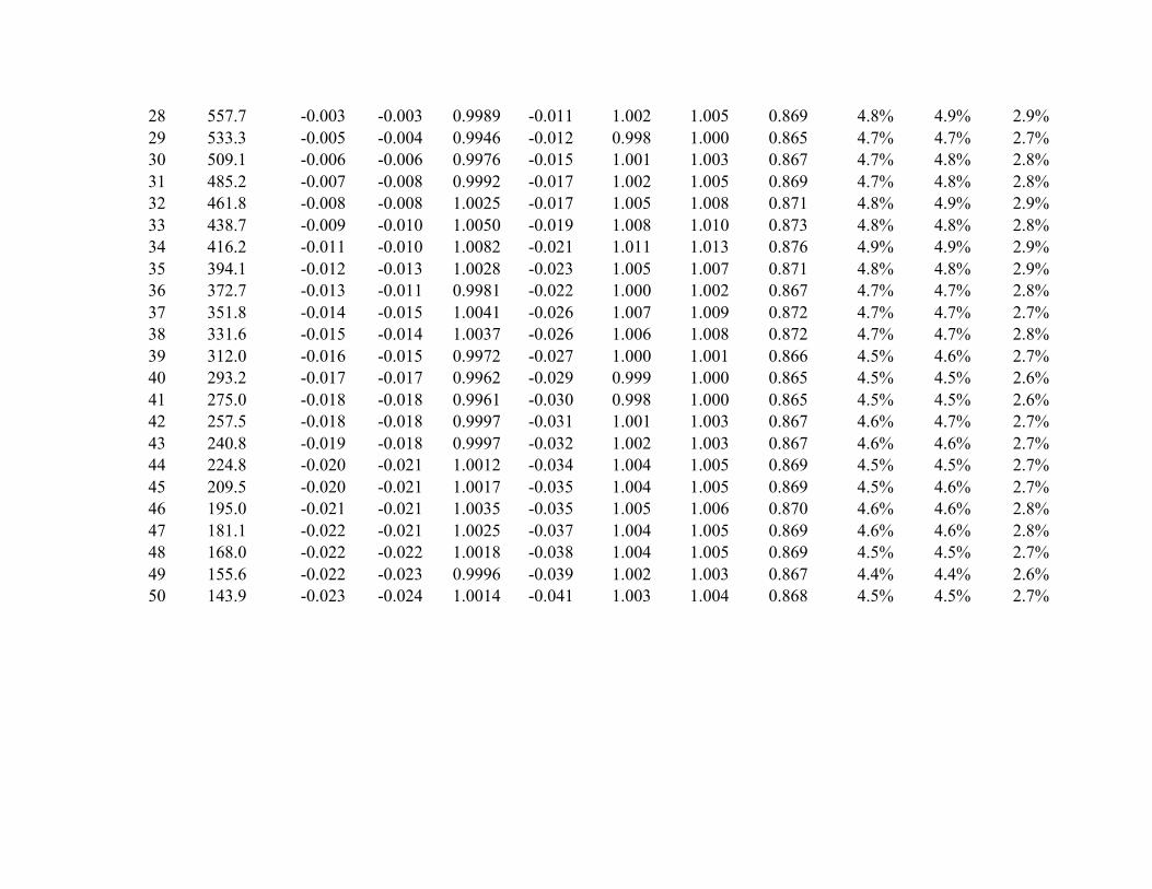
28 557.7 -0.003 -0.003 0.9989 -0.011 1.002 1.005 0.869 4.8% 4.9% 2.9% 29 533.3 -0.005 -0.004 0.9946 -0.012 0.998 1.000 0.865 4.7% 4.7% 2.7% 30 509.1 -0.006 -0.006 0.9976 -0.015 1.001 1.003 0.867 4.7% 4.8% 2.8% 31 485.2 -0.007 -0.008 0.9992 -0.017 1.002 1.005 0.869 4.7% 4.8% 2.8% 32 461.8 -0.008 -0.008 1.0025 -0.017 1.005 1.008 0.871 4.8% 4.9% 2.9% 33 438.7 -0.009 -0.010 1.0050 -0.019 1.008 1.010 0.873 4.8% 4.8% 2.8% 34 416.2 -0.011 -0.010 1.0082 -0.021 1.011 1.013 0.876 4.9% 4.9% 2.9% 35 394.1 -0.012 -0.013 1.0028 -0.023 1.005 1.007 0.871 4.8% 4.8% 2.9% 36 372.7 -0.013 -0.011 0.9981 -0.022 1.000 1.002 0.867 4.7% 4.7% 2.8% 37 351.8 -0.014 -0.015 1.0041 -0.026 1.007 1.009 0.872 4.7% 4.7% 2.7% 38 331.6 -0.015 -0.014 1.0037 -0.026 1.006 1.008 0.872 4.7% 4.7% 2.8% 39 312.0 -0.016 -0.015 0.9972 -0.027 1.000 1.001 0.866 4.5% 4.6% 2.7% 40 293.2 -0.017 -0.017 0.9962 -0.029 0.999 1.000 0.865 4.5% 4.5% 2.6% 41 275.0 -0.018 -0.018 0.9961 -0.030 0.998 1.000 0.865 4.5% 4.5% 2.6% 42 257.5 -0.018 -0.018 0.9997 -0.031 1.001 1.003 0.867 4.6% 4.7% 2.7% 43 240.8 -0.019 -0.018 0.9997 -0.032 1.002 1.003 0.867 4.6% 4.6% 2.7% 44 224.8 -0.020 -0.021 1.0012 -0.034 1.004 1.005 0.869 4.5% 4.5% 2.7% 45 209.5 -0.020 -0.021 1.0017 -0.035 1.004 1.005 0.869 4.5% 4.6% 2.7% 46 195.0 -0.021 -0.021 1.0035 -0.035 1.005 1.006 0.870 4.6% 4.6% 2.8% 47 181.1 -0.022 -0.021 1.0025 -0.037 1.004 1.005 0.869 4.6% 4.6% 2.8% 48 168.0 -0.022 -0.022 1.0018 -0.038 1.004 1.005 0.869 4.5% 4.5% 2.7% 49 155.6 -0.022 -0.023 0.9996 -0.039 1.002 1.003 0.867 4.4% 4.4% 2.6% 50 143.9 -0.023 -0.024 1.0014 -0.041 1.003 1.004 0.868 4.5% 4.5% 2.7%

Table 1 (continued)

Panel B: Sample Size generated for each simulation trial = 4,000


Known Probabilities


Estimated Probabilities

Std. Diff. Using BD

Std. Diff. Using BMN

Variance Effective Level of 5%

Significance Test

Interval

Interval Expected

n

Theoretical Expectation

of Std. Diff. Mean

Standard Dev. Mean

Standard Dev.

Standard Dev.

Standard Dev.

Based on Estimated

Probs. Using BD

Using BMN

Variance (1) (2) (3) (4) (5) (6) (7) (8) (9) (10) (11) (12)

-50 9.0 -0.006 -0.007 0.9996 -0.078 1.018 1.019 0.868 3.6% 3.6% 2.5% -49 9.7 -0.006 -0.005 0.9991 -0.073 1.016 1.017 0.868 3.6% 3.6% 2.5% -48 10.5 -0.006 -0.006 0.9989 -0.071 1.014 1.015 0.867 3.7% 3.7% 2.4% -47 11.3 -0.005 -0.004 0.9987 -0.067 1.013 1.014 0.867 3.7% 3.7% 2.4% -46 12.2 -0.005 -0.006 0.9971 -0.066 1.011 1.012 0.866 3.8% 3.8% 2.4% -45 13.1 -0.005 -0.005 0.9987 -0.063 1.012 1.013 0.868 3.8% 3.8% 2.5% -44 14.0 -0.005 -0.005 0.9993 -0.061 1.012 1.013 0.868 3.9% 3.9% 2.5% -43 15.0 -0.005 -0.005 1.0007 -0.059 1.012 1.014 0.869 4.0% 4.0% 2.5% -42 16.1 -0.005 -0.004 0.9993 -0.056 1.011 1.012 0.868 4.0% 4.0% 2.5% -41 17.2 -0.004 -0.004 0.9998 -0.054 1.011 1.012 0.869 4.0% 4.0% 2.5% -40 18.3 -0.004 -0.005 1.0011 -0.054 1.012 1.013 0.870 4.1% 4.1% 2.5% -39 19.5 -0.004 -0.004 0.9992 -0.050 1.009 1.010 0.868 4.1% 4.1% 2.5% -38 20.7 -0.004 -0.003 0.9998 -0.049 1.009 1.011 0.869 4.1% 4.1% 2.6% -37 22.0 -0.003 -0.004 1.0017 -0.048 1.011 1.013 0.871 4.2% 4.2% 2.6% -36 23.3 -0.003 -0.003 1.0012 -0.046 1.010 1.012 0.870 4.2% 4.2% 2.6% -35 24.6 -0.003 -0.003 1.0014 -0.045 1.010 1.012 0.871 4.2% 4.2% 2.6% -34 26.0 -0.003 -0.002 1.0018 -0.043 1.010 1.012 0.871 4.2% 4.2% 2.6% -33 27.4 -0.002 -0.001 1.0015 -0.041 1.010 1.012 0.871 4.2% 4.2% 2.7% -32 28.9 -0.002 -0.004 1.0009 -0.043 1.009 1.011 0.871 4.2% 4.2% 2.6%

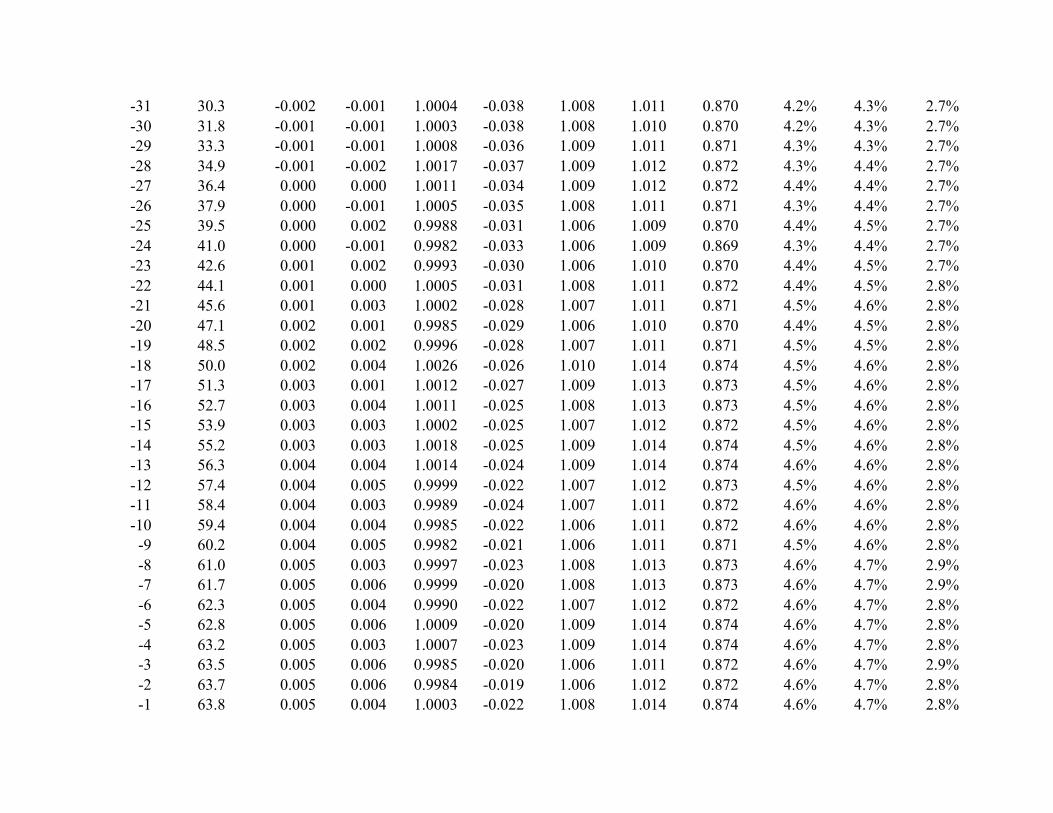
-31 30.3 -0.002 -0.001 1.0004 -0.038 1.008 1.011 0.870 4.2% 4.3% 2.7% -30 31.8 -0.001 -0.001 1.0003 -0.038 1.008 1.010 0.870 4.2% 4.3% 2.7% -29 33.3 -0.001 -0.001 1.0008 -0.036 1.009 1.011 0.871 4.3% 4.3% 2.7% -28 34.9 -0.001 -0.002 1.0017 -0.037 1.009 1.012 0.872 4.3% 4.4% 2.7% -27 36.4 0.000 0.000 1.0011 -0.034 1.009 1.012 0.872 4.4% 4.4% 2.7% -26 37.9 0.000 -0.001 1.0005 -0.035 1.008 1.011 0.871 4.3% 4.4% 2.7% -25 39.5 0.000 0.002 0.9988 -0.031 1.006 1.009 0.870 4.4% 4.5% 2.7% -24 41.0 0.000 -0.001 0.9982 -0.033 1.006 1.009 0.869 4.3% 4.4% 2.7% -23 42.6 0.001 0.002 0.9993 -0.030 1.006 1.010 0.870 4.4% 4.5% 2.7% -22 44.1 0.001 0.000 1.0005 -0.031 1.008 1.011 0.872 4.4% 4.5% 2.8% -21 45.6 0.001 0.003 1.0002 -0.028 1.007 1.011 0.871 4.5% 4.6% 2.8% -20 47.1 0.002 0.001 0.9985 -0.029 1.006 1.010 0.870 4.4% 4.5% 2.8% -19 48.5 0.002 0.002 0.9996 -0.028 1.007 1.011 0.871 4.5% 4.5% 2.8% -18 50.0 0.002 0.004 1.0026 -0.026 1.010 1.014 0.874 4.5% 4.6% 2.8% -17 51.3 0.003 0.001 1.0012 -0.027 1.009 1.013 0.873 4.5% 4.6% 2.8% -16 52.7 0.003 0.004 1.0011 -0.025 1.008 1.013 0.873 4.5% 4.6% 2.8% -15 53.9 0.003 0.003 1.0002 -0.025 1.007 1.012 0.872 4.5% 4.6% 2.8% -14 55.2 0.003 0.003 1.0018 -0.025 1.009 1.014 0.874 4.5% 4.6% 2.8% -13 56.3 0.004 0.004 1.0014 -0.024 1.009 1.014 0.874 4.6% 4.6% 2.8% -12 57.4 0.004 0.005 0.9999 -0.022 1.007 1.012 0.873 4.5% 4.6% 2.8% -11 58.4 0.004 0.003 0.9989 -0.024 1.007 1.011 0.872 4.6% 4.6% 2.8% -10 59.4 0.004 0.004 0.9985 -0.022 1.006 1.011 0.872 4.6% 4.6% 2.8%

-9 60.2 0.004 0.005 0.9982 -0.021 1.006 1.011 0.871 4.5% 4.6% 2.8% -8 61.0 0.005 0.003 0.9997 -0.023 1.008 1.013 0.873 4.6% 4.7% 2.9% -7 61.7 0.005 0.006 0.9999 -0.020 1.008 1.013 0.873 4.6% 4.7% 2.9% -6 62.3 0.005 0.004 0.9990 -0.022 1.007 1.012 0.872 4.6% 4.7% 2.8% -5 62.8 0.005 0.006 1.0009 -0.020 1.009 1.014 0.874 4.6% 4.7% 2.8% -4 63.2 0.005 0.003 1.0007 -0.023 1.009 1.014 0.874 4.6% 4.7% 2.8% -3 63.5 0.005 0.006 0.9985 -0.020 1.006 1.011 0.872 4.6% 4.7% 2.9% -2 63.7 0.005 0.006 0.9984 -0.019 1.006 1.012 0.872 4.6% 4.7% 2.8% -1 63.8 0.005 0.004 1.0003 -0.022 1.008 1.014 0.874 4.6% 4.7% 2.8%

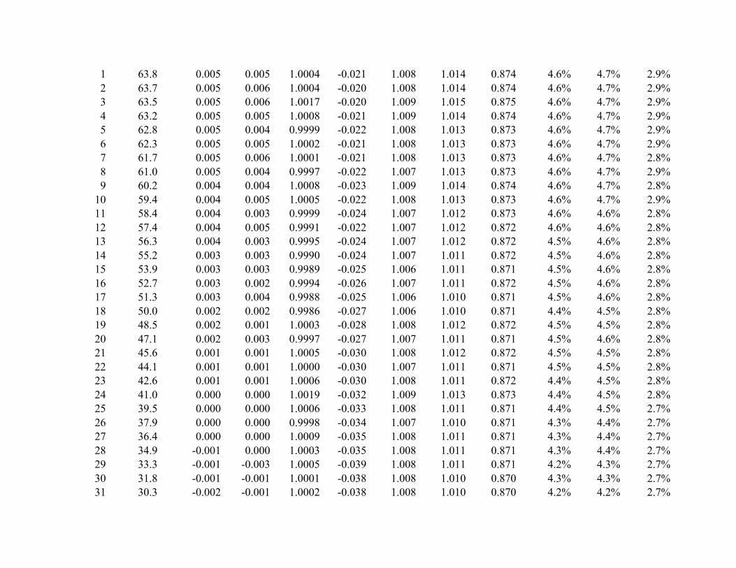
1 63.8 0.005 0.005 1.0004 -0.021 1.008 1.014 0.874 4.6% 4.7% 2.9% 2 63.7 0.005 0.006 1.0004 -0.020 1.008 1.014 0.874 4.6% 4.7% 2.9% 3 63.5 0.005 0.006 1.0017 -0.020 1.009 1.015 0.875 4.6% 4.7% 2.9% 4 63.2 0.005 0.005 1.0008 -0.021 1.009 1.014 0.874 4.6% 4.7% 2.9% 5 62.8 0.005 0.004 0.9999 -0.022 1.008 1.013 0.873 4.6% 4.7% 2.9% 6 62.3 0.005 0.005 1.0002 -0.021 1.008 1.013 0.873 4.6% 4.7% 2.9% 7 61.7 0.005 0.006 1.0001 -0.021 1.008 1.013 0.873 4.6% 4.7% 2.8% 8 61.0 0.005 0.004 0.9997 -0.022 1.007 1.013 0.873 4.6% 4.7% 2.9% 9 60.2 0.004 0.004 1.0008 -0.023 1.009 1.014 0.874 4.6% 4.7% 2.8%

10 59.4 0.004 0.005 1.0005 -0.022 1.008 1.013 0.873 4.6% 4.7% 2.9% 11 58.4 0.004 0.003 0.9999 -0.024 1.007 1.012 0.873 4.6% 4.6% 2.8% 12 57.4 0.004 0.005 0.9991 -0.022 1.007 1.012 0.872 4.6% 4.6% 2.8% 13 56.3 0.004 0.003 0.9995 -0.024 1.007 1.012 0.872 4.5% 4.6% 2.8% 14 55.2 0.003 0.003 0.9990 -0.024 1.007 1.011 0.872 4.5% 4.6% 2.8% 15 53.9 0.003 0.003 0.9989 -0.025 1.006 1.011 0.871 4.5% 4.6% 2.8% 16 52.7 0.003 0.002 0.9994 -0.026 1.007 1.011 0.872 4.5% 4.6% 2.8% 17 51.3 0.003 0.004 0.9988 -0.025 1.006 1.010 0.871 4.5% 4.6% 2.8% 18 50.0 0.002 0.002 0.9986 -0.027 1.006 1.010 0.871 4.4% 4.5% 2.8% 19 48.5 0.002 0.001 1.0003 -0.028 1.008 1.012 0.872 4.5% 4.5% 2.8% 20 47.1 0.002 0.003 0.9997 -0.027 1.007 1.011 0.871 4.5% 4.6% 2.8% 21 45.6 0.001 0.001 1.0005 -0.030 1.008 1.012 0.872 4.5% 4.5% 2.8% 22 44.1 0.001 0.001 1.0000 -0.030 1.007 1.011 0.871 4.5% 4.5% 2.8% 23 42.6 0.001 0.001 1.0006 -0.030 1.008 1.011 0.872 4.4% 4.5% 2.8% 24 41.0 0.000 0.000 1.0019 -0.032 1.009 1.013 0.873 4.4% 4.5% 2.8% 25 39.5 0.000 0.000 1.0006 -0.033 1.008 1.011 0.871 4.4% 4.5% 2.7% 26 37.9 0.000 0.000 0.9998 -0.034 1.007 1.010 0.871 4.3% 4.4% 2.7% 27 36.4 0.000 0.000 1.0009 -0.035 1.008 1.011 0.871 4.3% 4.4% 2.7% 28 34.9 -0.001 0.000 1.0003 -0.035 1.008 1.011 0.871 4.3% 4.4% 2.7% 29 33.3 -0.001 -0.003 1.0005 -0.039 1.008 1.011 0.871 4.2% 4.3% 2.7% 30 31.8 -0.001 -0.001 1.0001 -0.038 1.008 1.010 0.870 4.3% 4.3% 2.7% 31 30.3 -0.002 -0.001 1.0002 -0.038 1.008 1.010 0.870 4.2% 4.2% 2.7%

32 28.9 -0.002 -0.001 1.0023 -0.040 1.010 1.013 0.872 4.2% 4.2% 2.7% 33 27.4 -0.002 -0.003 1.0006 -0.043 1.009 1.011 0.870 4.2% 4.2% 2.6% 34 26.0 -0.003 -0.003 0.9994 -0.044 1.008 1.010 0.869 4.1% 4.1% 2.6% 35 24.6 -0.003 -0.003 0.9998 -0.045 1.008 1.010 0.869 4.1% 4.1% 2.6% 36 23.3 -0.003 -0.002 1.0011 -0.045 1.010 1.012 0.870 4.1% 4.1% 2.6% 37 22.0 -0.003 -0.005 1.0001 -0.049 1.009 1.011 0.869 4.1% 4.1% 2.6% 38 20.7 -0.004 -0.003 0.9995 -0.049 1.009 1.011 0.869 4.1% 4.1% 2.5% 39 19.5 -0.004 -0.004 1.0000 -0.051 1.010 1.011 0.869 4.1% 4.1% 2.5% 40 18.3 -0.004 -0.004 1.0005 -0.052 1.011 1.012 0.869 4.1% 4.1% 2.5% 41 17.2 -0.004 -0.006 1.0005 -0.056 1.011 1.013 0.869 4.1% 4.1% 2.5% 42 16.1 -0.005 -0.004 1.0002 -0.056 1.012 1.013 0.869 4.0% 4.0% 2.5% 43 15.0 -0.005 -0.004 0.9983 -0.057 1.010 1.011 0.867 3.9% 3.9% 2.5% 44 14.0 -0.005 -0.006 1.0001 -0.062 1.013 1.014 0.869 3.9% 3.9% 2.5% 45 13.1 -0.005 -0.005 1.0022 -0.063 1.015 1.016 0.870 3.9% 3.9% 2.5% 46 12.2 -0.005 -0.005 1.0021 -0.065 1.016 1.017 0.870 3.9% 3.9% 2.5% 47 11.3 -0.005 -0.005 1.0020 -0.068 1.017 1.018 0.870 3.8% 3.8% 2.5% 48 10.5 -0.006 -0.006 0.9999 -0.071 1.016 1.017 0.868 3.7% 3.7% 2.4% 49 9.7 -0.006 -0.006 0.9992 -0.074 1.017 1.017 0.868 3.6% 3.6% 2.4% 50 9.0 -0.006 -0.005 0.9994 -0.076 1.018 1.019 0.868 3.6% 3.6% 2.4%

Table 2 Power of Standardized Difference Tests

For Various Sample Sizes and Rates of Earnings Management With Earnings Management Concentrated Entirely in Intervals –1 and +1

Panel A : Power of Left Standardized Differences

Sample Size

1,000 2,000 4,000 8,000 16,000 32,000 64,000 128,000

Rate 0.025 0.061 0.066 0.074 0.085 0.105 0.137 0.193 0.294

0.050 0.074 0.086 0.105 0.138 0.195 0.296 0.470 0.717 0.075 0.089 0.110 0.146 0.210 0.323 0.512 0.765 0.956 0.100 0.106 0.139 0.198 0.301 0.478 0.727 0.938 0.998 0.200 0.204 0.312 0.495 0.747 0.948 0.999 1.000 1.000 0.300 0.351 0.555 0.810 0.973 1.000 1.000 1.000 1.000 0.400 0.536 0.791 0.966 0.999 1.000 1.000 1.000 1.000 0.500 0.725 0.936 0.998 1.000 1.000 1.000 1.000 1.000 0.600 0.874 0.989 1.000 1.000 1.000 1.000 1.000 1.000 0.700 0.959 0.999 1.000 1.000 1.000 1.000 1.000 1.000 0.800 0.992 1.000 1.000 1.000 1.000 1.000 1.000 1.000 0.900 0.999 1.000 1.000 1.000 1.000 1.000 1.000 1.000

Panel B : Power of Right Standardized Differences 0.025 0.061 0.066 0.073 0.085 0.104 0.136 0.191 0.289

0.050 0.073 0.085 0.103 0.135 0.189 0.287 0.454 0.698 0.075 0.087 0.107 0.141 0.201 0.307 0.487 0.738 0.943 0.100 0.103 0.133 0.187 0.282 0.447 0.689 0.916 0.996 0.200 0.182 0.274 0.434 0.672 0.905 0.994 1.000 1.000 0.300 0.287 0.456 0.700 0.922 0.996 1.000 1.000 1.000 0.400 0.409 0.640 0.882 0.991 1.000 1.000 1.000 1.000 0.500 0.536 0.791 0.966 0.999 1.000 1.000 1.000 1.000 0.600 0.654 0.893 0.993 1.000 1.000 1.000 1.000 1.000 0.700 0.756 0.952 0.999 1.000 1.000 1.000 1.000 1.000 0.800 0.837 0.981 1.000 1.000 1.000 1.000 1.000 1.000 0.900 0.897 0.993 1.000 1.000 1.000 1.000 1.000 1.000

Power represents the probability (rounded to three decimal places of accuracy) of significant left-‐ or right-‐standardized differences for tests of level α=.05.

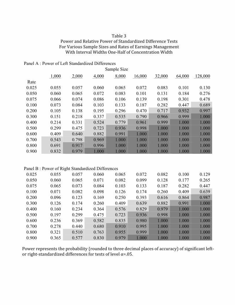
Table 3

Power and Relative Power of Standardized Difference Tests For Various Sample Sizes and Rates of Earnings Management

With Interval Widths One-‐Half of Concentration Width Panel A : Power of Left Standardized Differences

Sample Size

1,000 2,000 4,000 8,000 16,000 32,000 64,000 128,000

Rate 0.025 0.055 0.057 0.060 0.065 0.072 0.083 0.101 0.130

0.050 0.060 0.065 0.072 0.083 0.101 0.131 0.184 0.276 0.075 0.066 0.074 0.086 0.106 0.139 0.198 0.301 0.478 0.100 0.073 0.084 0.103 0.133 0.187 0.282 0.447 0.689 0.200 0.105 0.138 0.195 0.296 0.470 0.717 0.932 0.997 0.300 0.151 0.218 0.337 0.535 0.790 0.966 0.999 1.000 0.400 0.214 0.331 0.524 0.779 0.961 0.999 1.000 1.000 0.500 0.299 0.475 0.723 0.936 0.998 1.000 1.000 1.000 0.600 0.409 0.640 0.882 0.991 1.000 1.000 1.000 1.000 0.700 0.543 0.798 0.969 1.000 1.000 1.000 1.000 1.000 0.800 0.691 0.917 0.996 1.000 1.000 1.000 1.000 1.000 0.900 0.832 0.979 1.000 1.000 1.000 1.000 1.000 1.000

Panel B : Power of Right Standardized Differences

0.025 0.055 0.057 0.060 0.065 0.072 0.082 0.100 0.129 0.050 0.060 0.065 0.071 0.082 0.099 0.128 0.177 0.265 0.075 0.065 0.073 0.084 0.103 0.133 0.187 0.282 0.447 0.100 0.071 0.082 0.098 0.126 0.174 0.260 0.409 0.639 0.200 0.096 0.123 0.169 0.250 0.393 0.616 0.864 0.987 0.300 0.126 0.174 0.260 0.409 0.639 0.882 0.991 1.000 0.400 0.160 0.234 0.364 0.576 0.829 0.979 1.000 1.000 0.500 0.197 0.299 0.475 0.723 0.936 0.998 1.000 1.000 0.600 0.236 0.369 0.582 0.835 0.980 1.000 1.000 1.000 0.700 0.278 0.440 0.680 0.910 0.995 1.000 1.000 1.000 0.800 0.321 0.510 0.763 0.955 0.999 1.000 1.000 1.000 0.900 0.365 0.577 0.830 0.979 1.000 1.000 1.000 1.000


Table 3 (continued) Panel C : Relative Power of Left Standardized Differences

Sample Size

1,000 2,000 4,000 8,000 16,000 32,000 64,000 128,000

Rate 0.025 90% 87% 82% 76% 69% 61% 52% 44%

0.050 82% 76% 69% 61% 52% 44% 39% 39% 0.075 75% 67% 59% 51% 43% 39% 39% 50% 0.100 69% 60% 52% 44% 39% 39% 48% 69% 0.200 52% 44% 39% 40% 50% 72% 93% 100% 0.300 43% 39% 42% 55% 79% 97% 100% 100% 0.400 40% 42% 54% 78% 96% 100% 100% 100% 0.500 41% 51% 72% 94% 100% 100% 100% 100% 0.600 47% 65% 88% 99% 100% 100% 100% 100% 0.700 57% 80% 97% 100% 100% 100% 100% 100% 0.800 70% 92% 100% 100% 100% 100% 100% 100% 0.900 83% 98% 100% 100% 100% 100% 100% 100%

Panel D : Relative Power of Right Standardized Differences

0.025 90% 87% 82% 76% 69% 61% 52% 45% 0.050 82% 76% 69% 61% 52% 45% 39% 38% 0.075 75% 68% 60% 51% 43% 38% 38% 47% 0.100 69% 61% 53% 45% 39% 38% 45% 64% 0.200 53% 45% 39% 37% 43% 62% 86% 99% 0.300 44% 38% 37% 44% 64% 88% 99% 100% 0.400 39% 37% 41% 58% 83% 98% 100% 100% 0.500 37% 38% 49% 72% 94% 100% 100% 100% 0.600 36% 41% 59% 84% 98% 100% 100% 100% 0.700 37% 46% 68% 91% 100% 100% 100% 100% 0.800 38% 52% 76% 95% 100% 100% 100% 100% 0.900 41% 58% 83% 98% 100% 100% 100% 100%

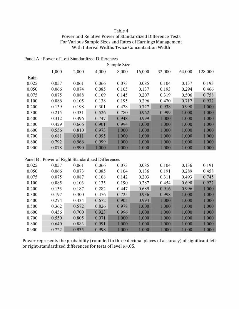
Table 4 Power and Relative Power of Standardized Difference Tests For Various Sample Sizes and Rates of Earnings Management

With Interval Widths Twice Concentration Width Panel A : Power of Left Standardized Differences

Sample Size

1,000 2,000 4,000 8,000 16,000 32,000 64,000 128,000

Rate 0.025 0.057 0.061 0.066 0.073 0.085 0.104 0.137 0.193

0.050 0.066 0.074 0.085 0.105 0.137 0.193 0.294 0.466 0.075 0.075 0.088 0.109 0.145 0.207 0.319 0.506 0.758 0.100 0.086 0.105 0.138 0.195 0.296 0.470 0.717 0.932 0.200 0.139 0.198 0.301 0.478 0.727 0.938 0.998 1.000 0.300 0.215 0.331 0.526 0.780 0.962 0.999 1.000 1.000 0.400 0.312 0.496 0.747 0.948 0.999 1.000 1.000 1.000 0.500 0.429 0.666 0.901 0.994 1.000 1.000 1.000 1.000 0.600 0.556 0.810 0.973 1.000 1.000 1.000 1.000 1.000 0.700 0.681 0.911 0.995 1.000 1.000 1.000 1.000 1.000 0.800 0.792 0.966 0.999 1.000 1.000 1.000 1.000 1.000 0.900 0.878 0.990 1.000 1.000 1.000 1.000 1.000 1.000

Panel B : Power of Right Standardized Differences 0.025 0.057 0.061 0.066 0.073 0.085 0.104 0.136 0.191

0.050 0.066 0.073 0.085 0.104 0.136 0.191 0.289 0.458 0.075 0.075 0.087 0.108 0.142 0.203 0.311 0.493 0.745 0.100 0.085 0.103 0.135 0.190 0.287 0.454 0.698 0.922 0.200 0.133 0.187 0.282 0.447 0.689 0.916 0.996 1.000 0.300 0.197 0.300 0.476 0.725 0.936 0.998 1.000 1.000 0.400 0.274 0.434 0.672 0.905 0.994 1.000 1.000 1.000 0.500 0.362 0.572 0.826 0.978 1.000 1.000 1.000 1.000 0.600 0.456 0.700 0.923 0.996 1.000 1.000 1.000 1.000 0.700 0.550 0.805 0.971 1.000 1.000 1.000 1.000 1.000 0.800 0.640 0.883 0.991 1.000 1.000 1.000 1.000 1.000 0.900 0.722 0.935 0.998 1.000 1.000 1.000 1.000 1.000


Table 4 (continued) Panel C : Relative Power of Left Standardized Differences

Sample Size

1,000 2,000 4,000 8,000 16,000 32,000 64,000 128,000

Rate 0.025 94% 92% 90% 86% 81% 76% 71% 66%

0.050 89% 86% 81% 76% 70% 65% 63% 65% 0.075 85% 80% 75% 69% 64% 62% 66% 79% 0.100 81% 75% 70% 65% 62% 65% 76% 93% 0.200 68% 63% 61% 64% 77% 94% 100% 100% 0.300 61% 60% 65% 80% 96% 100% 100% 100% 0.400 58% 63% 77% 95% 100% 100% 100% 100% 0.500 59% 71% 90% 99% 100% 100% 100% 100% 0.600 64% 82% 97% 100% 100% 100% 100% 100% 0.700 71% 91% 100% 100% 100% 100% 100% 100% 0.800 80% 97% 100% 100% 100% 100% 100% 100% 0.900 88% 99% 100% 100% 100% 100% 100% 100%

Panel D : Relative Power of Right Standardized Differences 0.025 95% 93% 90% 86% 82% 77% 71% 66%

0.050 90% 86% 82% 77% 72% 67% 64% 66% 0.075 86% 82% 76% 71% 66% 64% 67% 79% 0.100 83% 78% 72% 67% 64% 66% 76% 93% 0.200 73% 68% 65% 67% 76% 92% 100% 100% 0.300 69% 66% 68% 79% 94% 100% 100% 100% 0.400 67% 68% 76% 91% 99% 100% 100% 100% 0.500 68% 72% 86% 98% 100% 100% 100% 100% 0.600 70% 78% 93% 100% 100% 100% 100% 100% 0.700 73% 85% 97% 100% 100% 100% 100% 100% 0.800 76% 90% 99% 100% 100% 100% 100% 100% 0.900 80% 94% 100% 100% 100% 100% 100% 100%

Detecting Earnings Management Using Discontinuity … · Detecting Earnings Management Using...

Documents

Transcript of Detecting Earnings Management Using Discontinuity … · Detecting Earnings Management Using...