Detecting Changes in Student Behaviorfrom Clickstream Data

Jihyun ParkDepartment of Computer Science

University of California, IrvineIrvine, CA 92697

jihyunp@ics.uci.edu

Kameryn DenaroTeaching and Learning

Research CenterUniversity of California, Irvine

Irvine, CA 92697kdenaro@uci.edu

Fernando RodriguezSchool of Education

University of California, IrvineIrvine, CA 92697

fernanr1@uci.edu

Padhraic SmythDepartment of Computer Science

University of California, IrvineIrvine, CA 92697

smyth@ics.uci.edu

Mark WarschauerSchool of Education

University of California, IrvineIrvine, CA 92697

markw@uci.edu

ABSTRACTStudent clickstream data can provide valuable insights aboutstudent activities in an online learning environment and howthese activities inform their learning outcomes. However,given the noisy and complex nature of this data, an on-going challenge involves devising statistical techniques thatcapture clear and meaningful aspects of students’ click pat-terns. In this paper, we utilize statistical change detectiontechniques to investigate students’ online behaviors. Us-ing clickstream data from two large university courses, oneface-to-face and one online, we illustrate how this method-ology can be used to detect when students change their pre-viewing and reviewing behavior, and how these changes canbe related to other aspects of students’ activity and perfor-mance.

CCS Concepts•Information systems→ Data mining; Web log anal-ysis; •Computing methodologies → Machine learn-ing approaches; •Applied computing→ Learning man-agement systems;

KeywordsStudent clickstream data; Change detection; Regression; Pois-son models

1. INTRODUCTIONOne of the major goals in educational data mining (EDM)

is to use student clickstream data to describe and under-stand students’ behavioral patterns. While past findings

Permission to make digital or hard copies of all or part of this work for personal orclassroom use is granted without fee provided that copies are not made or distributedfor profit or commercial advantage and that copies bear this notice and the full cita-tion on the first page. Copyrights for components of this work owned by others thanACM must be honored. Abstracting with credit is permitted. To copy otherwise, or re-publish, to post on servers or to redistribute to lists, requires prior specific permissionand/or a fee. Request permissions from permissions@acm.org.

LAK ’17, March 13-17, 2017, Vancouver, BC, Canadac© 2017 ACM. ISBN 978-1-4503-4870-6/17/03. . . $15.00

DOI: http://dx.doi.org/10.1145/3027385.3027430

have advanced our understanding what we can learn fromclickstream data, one of the remaining challenges involvesdevising statistical techniques that help us identify studentswho are changing behavior in the middle of a term. Thereare a number of reasons motivating this problem; one isto identify students who are in need of assistance duringthe course, another is to identify reasons that students arechanging their behavior so that a course could be improvedoverall. The analysis of clickstream data within a course canalso provide invaluable information to course instructors andto education researchers, and there is a need to be able toboth summarize and visualize the results in a straightfor-ward manner.

In this paper we will focus on clickstream data from twocourses at a large university: one face-to-face course and oneonline course, both from the 2015-2016 academic year. Foreach course, clickstream data is obtained through a coursemanagement system in the form of {student ID, time stamp,activity}. The types of activities recorded correspond tobroad categories of student behavior, such as previewinglecture notes, submitting assignments, or posting and re-sponding to discussion board questions. For instance, oneof the courses we examine in this paper had 377 registeredstudents who generated approximately 380,000 click eventsover a 10-week period. Figure 1 displays each of the indi-vidual student clickstreams over the 85 days of the course,with each row corresponding to a student. While the plotshows some general increases in click activities around quizand exam dates, it is not easy to see much else, nor to un-derstand how individual student behaviors are related to theoverall population due to significant variability in students’click patterns. Furthermore, we are unable to determinewhether students change their click behaviors in any signif-icant way, or whether or not these behaviors are correlatedwith course performance.

As discussed in more detail in the next section, studentclickstream data has been the subject of a number of priorstudies, such as the investigation of potential predictive re-lationships between online student activity and student out-comes (such as course grades). Here we focus instead ondetecting changes in individual student activity over time,relative to the activity of the class of a whole. In particular

DAYS

STUDENTS

0

1

Figure 1: A plot of student clickstream activity inthe 10-week face-to-face course over time, whereeach row represents an individual student and eachcolumn represents a day. A black marker in cell i, tindicates clickstream activity for student i on day t.

we investigate the use of statistical change detection tech-niques (e.g., [9]) to automatically detect changes in activityover time for each student. We model the activity of eachstudent relative to the aggregate activity of all students inthe class and compare two models on a per student basis; amodel where there is no change in student activity versus amodel where there is a significant change in activity at someunknown point during the period of the course. Likelihood-based techniques are used to fit both models on a per studentbasis and model selection criteria is implemented in order todetermine whether each student is best modeled under the“change” or “no-change” model.

The paper proceeds as follows. In Section 2 we discuss re-lated work. Section 3 outlines the change-detection method-ology that we propose, and Section 4 provides illustrative re-sults on simulated data sets. Section 5 discusses the coursedata sets that provide an illustration of the methods dis-cussed in Section 3 and Section 6 describes the results ofapplying our change-detection methodology to these datasets. The paper concludes with discussion and conclusionsin Section 7. The primary novel contribution of this work isthe development of a systematic quantitative approach fordetecting significant changes in a student’s clickstream overtime.

2. RELATED WORKClickstream data analysis in an educational setting has fo-

cused on what the clickstream can say about the students interms of learning behavior through a variety of features de-rived from the clickstream. Much of the prior work on click-stream data analysis for understanding student behavior hasoccurred in the context of Massive Open Online Courses(MOOC) setting. Many of these analyses have focused onusing the clickstream data to predict MOOC completion (forexample in [5]) and to predict learning outcomes within aMOOC. For example, the relationship between the numberof posts and the learning gains of the students [16] has beeninvestigated, as well as how discussion forum views are po-tentially related to learning outcomes [1]. There has alsobeen research focused on improving predictions of learningoutcomes by incorporating clickstream events as well as sum-

maries of the clickstream [3].A secondary research topic has focused on describing stu-

dents with similar clickstreams (e.g., [15]), the activities thatthe students are engaging in, and in understanding the stu-dent’s typical online interaction within a class. As an exam-ple, clickstream data analysis was used to better understandwhether or not students were following a defined learningpath [6]. In other work, students’ clickstreams were groupedinto similar plans of action to better understand learningpathways [14]; how discussion forums and other activities inthe MOOC were related to country and culture [12]; and ex-amined whether engagement on discussion forums increasedbased on the type of video a student watched [2]. All ofthese clickstream analyses have an underlying goal of de-scribing student behaviors through the clickstream and todraw meaningful conclusions about those students.

MOOCs are typically used by people as a way to learnnew skills or keep up-to-date with current ones. Becausemost MOOCs do not offer formal degrees, there are no se-rious consequences for doing poorly or dropping out. Incontrast, college course grades determine whether studentssucceed or fail (whether they advance to the next course, re-main in their intended major, or graduate). Thus, findingsfrom MOOC clickstream studies cannot offer broad expla-nations about student learning experiences in higher educa-tion settings. So while MOOCs and college courses sharesome similarities, in terms of course management systemsand clickstream data, studying college courses may requirea different set of goals and statistical techniques.

For instance, one important area of higher education re-search focuses on student engagement. Studies find thatstudents who are not engaged with the learning process—that is, students who do not put in the time and energy intopurposeful learning—are at greater risk for failing coursesand dropping out of college [10]. While this finding is notnew, understanding how to quickly identify these students,especially at the course-level, remains a significant challenge.

Clickstream data has the potential to address this sincethe data is obtained in real time. Researchers can provideinstructors with immediate insights how students are engag-ing with the course management system. This is especiallyimportant in courses with large enrollments, where problemswith student engagement can often go unnoticed [13]. Somerecent work has found that student engagement with thecourse management system, as indexed by number of daysstudents visited the site relative to their peers, was positivelyrelated to course outcomes [11]. Our work adds to this areaof research by using statistical change detection techniquesto further understand course engagement.

More broadly, changepoint detection techniques for eventtime-series is a widely studied topic and a variety of statis-tical methodologies have been developed (e.g., [7, 9]), withmuch of this work focused on single (univariate) time-series.Web user behavior has been analyzed to detect changes inan individual’s behavior, to report“interesting”sessions, andto detect changes in user activity [8]. There has not beenany prior work (to our knowledge) on change detection ap-plied to multiple clickstreams of students in an educationalsetting.

Thus far, previous work in the analysis of clickstream datain an educational setting has focused on grouping studentsinto similar groups, understanding possible dropout, pre-dicting student success in a course, and defining learning

pathways. Our goal is to add to the current body of researchin a meaningful way by using changepoint detection tech-niques as a proxy for understanding student engagement.By detecting whether student behavior changes in a signif-icant manner over the time-period of a particular term, wehope to identify students who increase, decrease, or showno change in their clickstream activities, and whether thesechanges relate to course performance.

3. METHODOLOGYWe discuss below our approach for modeling and change

detection of student activity. We begin by defining somegeneral notation and then introduce two different models:a Bernoulli model for binary data and a Poisson model forcount data. The section concludes with a description ofchangepoint detection for both of these models.

3.1 NotationLet N be the number of individual students in a course

where i is an index that refers to an individual student inthe class, i = 1, . . . , N . We will assume below that time isdiscrete1 with T discrete time-points and t = 1, . . . , T beingan index running from the first to the last time-period ofclickstream logging for the course. Below we will refer tot on a daily time-scale for convenience but in general othertime-periods–such as days or weeks–could be used.

Let X be the observed data for a course, represented as anN×T array whose entries are counts xit ∈ {0, 1, 2, ....}. Notethat xit represents the number of click events for student i onday t, where 1 ≤ i ≤ N and 1 ≤ t ≤ T . We will also considera binarized version of the data x′it = I(xit > 0), where I()is an indicator function (as in Figure 1 for example). Thenumber of clicks xit (counts) by student i on a given dayt in principle contains more information than the binarizedversion x′it, but could also be quite noisy in the sense thatmore clicks might not necessarily correlate well with relevantstudent activity. We explore both options since the choiceof looking at a count versus the binarized version in practicewill depend on the context of a particular analysis.

3.2 Bernoulli Models for Binary DataFor the binary data, x′it, let πit be the probability that

each student i is active on day t (i.e., the probability thatstudent i generates one or more clicks on day t). The log-odds of πit is modeled as:

logπit

1− πit= µt + αi (1)

where µt, t = 1, . . . , T can be viewed as a time-varying popu-lation mean for the log-odds and αi, 1 ≤ i ≤ N is a student-dependent offset to account for individual-level variation instudent behavior.

The role of αi in this model is to modulate the time-varying population mean µt in a student-specific manner.A positive value of αi for student i will increase the log-odds above the population mean µt, which in turn meansthat student i tends to click more than the mean student asrepresented by µt. A negative value of αi has the oppositeeffect; student i has a lower probability of clicking compared

1A changepoint methodology using a continuous-time modelcould in principle also be developed in a manner similar tothe discrete-time methodology we describe in this paper.

0 10 20 30 40 50 60 70 80

DAYS

0.0

0.2

0.4

0.6

0.8

1.0

FR

AC

TIO

N O

F S

TU

DEN

TS

Figure 2: Proportion of students who click each dayduring a 10-week course.

0 10 20 30 40 50 60 70 80

DAYS

0

5

10

15

20

25

30

35

40

AV

ER

AG

E N

UM

BER

OF C

LIC

KS

EXAM

Figure 3: Average number of click events per stu-dent each day during a 10-week course.

to the average student. µt represents time-varying popula-tion behavior on a log-odds scale.

Our approach to change detection relies on modeling eachstudent’s activity relative to that of the overall student pop-ulation in the class. This population (or background) rate µtwill typically vary significantly as a function of time t sincestudent behavior is strongly affected by temporal effects suchas days of lectures, weekday versus weekend effects, assign-ment deadlines, exams, and so on. As an example, Figure 2shows the proportion of students who clicked on a file eachday, summarizing the data shown earlier in Figure 1.

Modeling the log-odds as a linear function (Equation 1)is a standard technique in generalized linear modeling andensures that the resulting probability πit above lies between0 and 1, i.e., Equation 1 above can be rewritten as

πit =1

1 + e−(µt+αi). (2)

3.3 Estimation of Model ParametersThe parameters µ = {µ1, . . . , µt} and α = {α1, . . . , αN}

are estimated from the N × T data array X ′ with entriesx′it ∈ {0, 1}, 1 ≤ i ≤ N, 1 ≤ t ≤ T . Since the x′it’s arebinary the likelihood for each individual data point x′it canbe written as:

L(µ, σ|x′it) = πx′itit (1− πit)(1−x

′it), (3)

where πit is defined in Equation 2. The likelihood of the fulldata set X ′ is then defined as:

L(µ, α|X ′) = P (X ′|µ, α)

=

N∏i=1

T∏t=1

πx′itit (1− πit)(1−x

′it). (4)

Here we make the assumption that the observed data for

each student on each day is conditionally independent of allother observations (for students and for days) given the pa-rameters µ and α. This is a simplification since it ignores(for example) possible time-varying trends in student be-havior. Nonetheless, as we will see later in the experimentalresults it provides a useful basis for change detection.

We use a two-stage procedure for parameter estimation asfollows2. We first generate an estimate µ̂t for the populationmean as follows:

µ̂t = logq̂t

1− q̂t, 1 ≤ t ≤ T (5)

where q̂t = 1N

∑Ni=1 x

′it, which is the proportion of students

(across all students) that generated a click on day t.In the second step, we fit a regression model for each stu-

dent i in Equation 1 with the population mean µ̂t set as anoffset. αi can be thought of as a student-specific interceptterm for each student i.

3.4 Poisson Models for Count DataWe can also model the counts xit directly, where xit can

have values {0, 1, 2, ...}. A natural model in this context isthe Poisson model.

We develop the count model in a manner similar to thatfor binary case earlier. In particular, we model the loga-rithm of the mean of the Poisson distribution, log λit as alinear function of a time-varying population rate µt and anindividual student effect αi:

log λit = µt + αi. (6)

Note that although for convenience we use the same nota-tion, µ and α, for our two sets of parameters, and they playan analogous role as their “namesake” parameters in the bi-nary model, these parameters are different from those in thebinary model described earlier.

Figure 3 shows the average number of click events for eachstudent per day, reflecting the type of time-varying popula-tion behavior that µt is intended to capture. The red dashedlines are the dates for the three midterms and the final, andwe can see much more click activities right before the examdates.

We can write the likelihood function for a single count xitas

P (xit|µt, αi) =λxitit e

−λit

xit!, (7)

where λit is defined in Equation 6. As with the binarycase, assuming that the observations xit are conditionallyindependent given the parameters, the full likelihood can bewritten as:

L(µ, α|X) = P (X|µ, α)

=

N∏i=1

T∏t=1

λxitit e−λit

xit!. (8)

We again make a conditional independence assumptionfor the Poisson model. A two-stage parameter estimationprocess is carried out as before. In the first step we estimateµ̂t as follows:

µ̂t = log m̂t, 1 ≤ t ≤ T (9)

2The estimation could be done in a single-step; we wouldexpect similar results to what we obtain in the two-stepapproach.

where m̂t = 1N

∑Ni=1 xit, representing the average number

of click events across the population that were generated onday t. In the second step we fit a Poisson regression modelfor each student i as in Equation 6 with an offset µ̂t to getan estimate for each αi.

3.5 Detecting Changes in ActivityTo detect changes in activity we allow for the possibility

that each student’s activity rate changes at some unknowntime point during the course. The proposed approach thatwe describe below works in the same manner for both theBernoulli binary model and the Poisson count model, theonly difference being in how the likelihood is defined andthe parameters are estimated for each (as described earlier).For simplicity, the reader can assume below that we areusing either the Bernoulli or Poisson model, and the issue iswhether to fit a model with a change or with no change.

We fit two different models for each student i. The firstmodel is the one where we assume that the student’s rateof activity αi, defined relative to the background activityµt, does not change over time. In the second model, thechangepoint model, we assume that a student’s activity rateswitches at some unknown changepoint. We fit both modelsto the data for each student and use a data-driven modelselection technique to select which model is justified giventhe observed data.

In the changepoint model we assume that there is one ac-tivity rate αi1 for student i before changepoint τi and a dif-ferent activity rate αi2 after the changepoint τi. The change-point model for binary data (for example) can be written asfollows, where I is an indicator function:

logπit

1− πit= µt + αi1I(t < τi) + αi2I(t > τi) (10)

with a similar definition for the Poisson model. We caninterpret this model as fitting two regression models withdifferent means on either side of the changepoint.

The value of the changepoint τi for each student is un-known. Since time t is discrete the values of τi can takeone of T − 1 possible values, corresponding to the T − 1boundaries between the T observation times.

In effect this changepoint model has 3 parameters (assum-ing µt is known): the two activity rates and the changepoint.We generate maximum likelihood estimates of these param-eters by maximizing the log-likelihood defined as follows (foreach student i)

li(αi1, αi2, τi, µ)

=∑t<τi

logP (x′it|αi1, µt) +∑t>τi

logP (x′it|αi2, µt) (11)

(with a similar equation for counts xit and the Poisson model).To fit this model, we use a similar two-stage approach as

for the model with no-change described earlier. In the firststage we fit the background rate µt using the data across allstudents, in the same manner as for the no-change model.In the second stage we find the values αi1, αi2, τi, for eachstudent i, that maximize the log-likelihood defined above.Since τi is discrete we can reduce the optimization problemto finding the values of αi1 and αi2 for a fixed τi and theniterate over the T − 1 possible values of τi. For each fixedvalue of τi, the log-likelihood splits into the two parts onthe right-hand side of Equation 11 above, a log-likelihoodterm containing αi1 and a second log-likelihood term con-

STUDENT1

0 10 20 30 40 50 60 70 80 90

DAYS

STUDENT2

Figure 4: Simulated activity data for two students.

taining αi2. Each can be optimized independently using thesame procedure described earlier for estimating αi for theno-change model.

For each student i, once the parameters of both the no-change and the changepoint models have been estimated,we select the best model from the two candidate models.The likelihood (or log-likelihood), evaluated at the maxi-mum likelihood values of the parameters, is not useful formodel selection since the changepoint model will always havea likelihood value that is at least as high as the no-changemodel (this is because the changepoint model contains theno-change model as a special case).

There are a variety of model selection techniques in thestatistical literature to handle the issue of how to fairlycompare models (in the case where models have differentnumbers of parameters) including techniques such as penal-ized likelihood, Bayesian criteria, and cross-validation [4].In the results in this paper we use the Bayesian Informa-tion Criterion (BIC) which is a well-established and easilyinterpretable method for model selection. The BIC score isdefined for each student as

BICiM = −2liM + pM log T (12)

where M indicates a particular model (M = 1 correspondsto the no-change model, and M = 2 corresponds to thechangepoint model), liM is the log-likelihood for model Mfor student i’s data evaluated at the maximum likelihoodvalues of the parameters, pM is the number of parametersin each model (p1 = 1, p2 = 3, for the no-change and change-point models respectively)3, and T is the number of obser-vations per student. The second term in the BIC, pM log T ,can be interpreted as a penalty for having additional param-eters in a model.

The BIC method selects the model with the lowest BICscore for each student. In particular, in the context of ourchangepoint application, we can use BIC to detect if thereis evidence that a student’s rate of activity changed, i.e., ifBICi2 < BICi1 then the evidence supports the changepointmodel over the no-change model for student i.

4. RESULTS FOR SIMULATED DATATo illustrate how the change-detection methods work, we

simulated daily binary time-series of student click activityfor 400 students over 85 days (numbers that are roughly sim-ilar to the larger of the two classes we analyze later in thepaper). The true population rate µt switched between twodifferent values over time, one with a high rate and one with

3Technically we should also count the background modelparameters µ here, but since this is the same for both modelswe can omit it.

0 5 10 15 20 25 30

DAYS

0.0

0.1

0.2

0.3

0.4

0.5

0.6

0.7

0.8

¼̂it

POPULATIONSTUDENT1 ®i=0.7

STUDENT2 ®i=-1.52

Figure 5: Estimated activity probabilities (π̂it) forthe two simulated students and for the population.

0 10 20 30 40 50 60 70 80−3.5

−3.0

−2.5

−2.0

−1.5

−1.0

−0.5

0.0

0.5

1.0

¹̂t+®̂i

M1, BIC=82.43

M2, BIC=75.74

0 10 20 30 40 50 60 70 80

DAYS

RAW DATA

DETECTED CP

TRUE CP

Figure 6: Log-odds of π̂it, for M1 and M2, and simu-lated data of a student with a changepoint at t = 57.

a low rate. The variability in the simulation roughly corre-sponds to what we observed in the real student data. Theoffsets, αij , for each student were sampled independentlyfrom a normal distribution; αij ∼ Normal(0, σ = 1.5). Halfof the students were simulated with one αi1, i.e. no changein behavior over time. The other half of the students hadtwo different offsets sampled, αi1 and αi2, on either side ofa changepoint τi which was sampled independently from auniform distribution; τi ∼ U(15, 70).

Figure 4 is a plot of binary data for two simulated studentswho did not have changepoints. Student 1 is much moreactive than Student 2, and therefore Student 1 is going tohave a larger estimated value for αi. The estimated πit’s forthese students over the first 30 days (time t = 1, ..., 30) isshown in Figure 5. The plot illustrates how the estimatedactivity varies relative to the population probability µt (thered solid curve). The more active student (green dashedline) has higher probabilities of clicking over time, while theless active student (blue dotted line) has lower probabilities,and both probabilities rise and fall relative to the behaviorof the population. For example, when student activity onaverage rises on a particular day such as day 10 (e.g., due toan assignment), the click probability for both students rises.

Next we show the results of two different simulated stu-dents, one with a changepoint and the other without a change-point. Figure 6 is a plot from a student with a changepoint,with the raw data in the lower plot and the fitted model(plotted on a log-odds scale) in the upper plot. There is aclear change in student behavior around day 59, and thisis visible both in the raw data (lower plot) and the fitted

0 10 20 30 40 50 60 70 80−2.5

−2.0

−1.5

−1.0

−0.5

0.0

0.5

¹̂t+®̂i

M1, BIC=86.96

M2, BIC=94.55

0 10 20 30 40 50 60 70 80

DAYS

RAW DATA

DETECTED CP

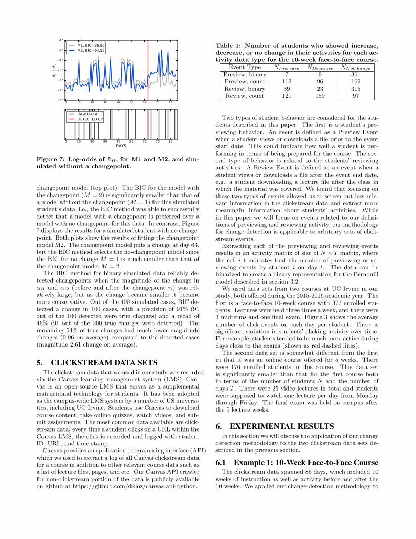
Figure 7: Log-odds of π̂it, for M1 and M2, and sim-ulated without a changepoint.

changepoint model (top plot). The BIC for the model withthe changepoint (M = 2) is significantly smaller than that ofa model without the changepoint (M = 1) for this simulatedstudent’s data, i.e., the BIC method was able to successfullydetect that a model with a changepoint is preferred over amodel with no changepoint for this data. In contrast, Figure7 displays the results for a simulated student with no change-point. Both plots show the results of fitting the changepointmodel M2. The changepoint model puts a change at day 63,but the BIC method selects the no-changepoint model sincethe BIC for no change M = 1 is much smaller than that ofthe changepoint model M = 2.

The BIC method for binary simulated data reliably de-tected changepoints when the magnitude of the change inαi1 and αi2 (before and after the changepoint τi) was rel-atively large, but as the change became smaller it becamemore conservative. Out of the 400 simulated cases, BIC de-tected a change in 100 cases, with a precision of 91% (91out of the 100 detected were true changes) and a recall of46% (91 out of the 200 true changes were detected). Theremaining 54% of true changes had much lower magnitudechanges (0.96 on average) compared to the detected cases(magnitude 2.61 change on average).

5. CLICKSTREAM DATA SETSThe clickstream data that we used in our study was recorded

via the Canvas learning management system (LMS). Can-vas is an open-source LMS that serves as a supplementalinstructional technology for students. It has been adoptedas the campus-wide LMS system by a number of US universi-ties, including UC Irvine. Students use Canvas to downloadcourse content, take online quizzes, watch videos, and sub-mit assignments. The most common data available are click-stream data; every time a student clicks on a URL within theCanvas LMS, the click is recorded and logged with studentID, URL, and time-stamp.

Canvas provides an application programming interface (API)which we used to extract a log of all Canvas clickstream datafor a course in addition to other relevant course data such asa list of lecture files, pages, and etc. Our Canvas API crawlerfor non-clickstream portion of the data is publicly availableon github at https://github.com/dkloz/canvas-api-python.

Table 1: Number of students who showed increase,decrease, or no change in their activities for each ac-tivity data type for the 10-week face-to-face course.

Event Type NIncrease NDecrease NNoChangePreview, binary 7 9 361Preview, count 112 96 169Review, binary 39 23 315Review, count 121 159 97

Two types of student behavior are considered for the stu-dents described in this paper. The first is a student’s pre-viewing behavior. An event is defined as a Preview Eventwhen a student views or downloads a file prior to the eventstart date. This could indicate how well a student is per-forming in terms of being prepared for the course. The sec-ond type of behavior is related to the students’ reviewingactivities. A Review Event is defined as an event when astudent views or downloads a file after the event end date,e.g., a student downloading a lecture file after the class inwhich the material was covered. We found that focusing onthese two types of events allowed us to screen out less rele-vant information in the clickstream data and extract moremeaningful information about students’ activities. Whilein this paper we will focus on events related to our defini-tions of previewing and reviewing activity, our methodologyfor change detection is applicable to arbitrary sets of click-stream events.

Extracting each of the previewing and reviewing eventsresults in an activity matrix of size of N × T matrix, wherethe cell i, t indicates that the number of previewing or re-viewing events by student i on day t. The data can bebinarized to create a binary representation for the Bernoullimodel described in section 3.2.

We used data sets from two courses at UC Irvine in ourstudy, both offered during the 2015-2016 academic year. Thefirst is a face-to-face 10-week course with 377 enrolled stu-dents. Lectures were held three times a week, and there were3 midterms and one final exam. Figure 3 shows the averagenumber of click events on each day per student. There issignificant variation in students’ clicking activity over time.For example, students tended to be much more active duringdays close to the exams (shown as red dashed lines).

The second data set is somewhat different from the firstin that it was an online course offered for 5 weeks. Therewere 176 enrolled students in this course. This data setis significantly smaller than that for the first course bothin terms of the number of students N and the number ofdays T . There were 25 video lectures in total and studentswere supposed to watch one lecture per day from Mondaythrough Friday. The final exam was held on campus afterthe 5 lecture weeks.

6. EXPERIMENTAL RESULTSIn this section we will discuss the application of our change

detection methodology to the two clickstream data sets de-scribed in the previous section.

6.1 Example 1: 10-Week Face-to-Face CourseThe clickstream data spanned 85 days, which included 10

weeks of instruction as well as activity before and after the10 weeks. We applied our change-detection methodology to

0 10 20 30 40 50 60 70 80DAYS

NInc

NDec

PREVIEW, COUNTS

0 10 20 30 40 50 60 70 80DAYS

NInc

NDec

REVIEW, COUNTS

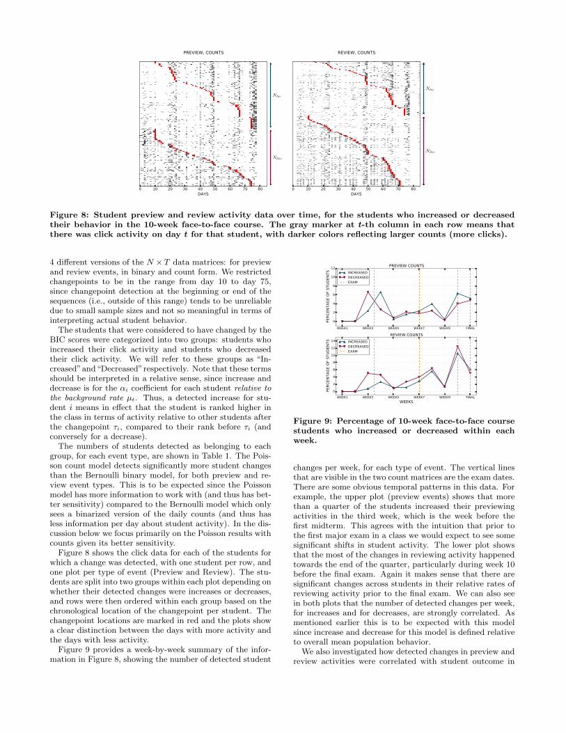
Figure 8: Student preview and review activity data over time, for the students who increased or decreasedtheir behavior in the 10-week face-to-face course. The gray marker at t-th column in each row means thatthere was click activity on day t for that student, with darker colors reflecting larger counts (more clicks).

4 different versions of the N × T data matrices: for previewand review events, in binary and count form. We restrictedchangepoints to be in the range from day 10 to day 75,since changepoint detection at the beginning or end of thesequences (i.e., outside of this range) tends to be unreliabledue to small sample sizes and not so meaningful in terms ofinterpreting actual student behavior.

The students that were considered to have changed by theBIC scores were categorized into two groups: students whoincreased their click activity and students who decreasedtheir click activity. We will refer to these groups as “In-creased”and“Decreased”respectively. Note that these termsshould be interpreted in a relative sense, since increase anddecrease is for the αi coefficient for each student relative tothe background rate µt. Thus, a detected increase for stu-dent i means in effect that the student is ranked higher inthe class in terms of activity relative to other students afterthe changepoint τi, compared to their rank before τi (andconversely for a decrease).

The numbers of students detected as belonging to eachgroup, for each event type, are shown in Table 1. The Pois-son count model detects significantly more student changesthan the Bernoulli binary model, for both preview and re-view event types. This is to be expected since the Poissonmodel has more information to work with (and thus has bet-ter sensitivity) compared to the Bernoulli model which onlysees a binarized version of the daily counts (and thus hasless information per day about student activity). In the dis-cussion below we focus primarily on the Poisson results withcounts given its better sensitivity.

Figure 8 shows the click data for each of the students forwhich a change was detected, with one student per row, andone plot per type of event (Preview and Review). The stu-dents are split into two groups within each plot depending onwhether their detected changes were increases or decreases,and rows were then ordered within each group based on thechronological location of the changepoint per student. Thechangepoint locations are marked in red and the plots showa clear distinction between the days with more activity andthe days with less activity.

Figure 9 provides a week-by-week summary of the infor-mation in Figure 8, showing the number of detected student

WEEK1 WEEK3 WEEK5 WEEK7 WEEK9 FINAL

0

2

4

6

8

10

12

PER

CEN

TA

GE O

F S

TU

DEN

TS

PREVIEW COUNTS

INCREASED

DECREASED

EXAM

WEEK1 WEEK3 WEEK5 WEEK7 WEEK9 FINAL

WEEKS

0

2

4

6

8

10

12

14

PER

CEN

TA

GE O

F S

TU

DEN

TS

REVIEW COUNTS

INCREASED

DECREASED

EXAM

Figure 9: Percentage of 10-week face-to-face coursestudents who increased or decreased within eachweek.

changes per week, for each type of event. The vertical linesthat are visible in the two count matrices are the exam dates.There are some obvious temporal patterns in this data. Forexample, the upper plot (preview events) shows that morethan a quarter of the students increased their previewingactivities in the third week, which is the week before thefirst midterm. This agrees with the intuition that prior tothe first major exam in a class we would expect to see somesignificant shifts in student activity. The lower plot showsthat the most of the changes in reviewing activity happenedtowards the end of the quarter, particularly during week 10before the final exam. Again it makes sense that there aresignificant changes across students in their relative rates ofreviewing activity prior to the final exam. We can also seein both plots that the number of detected changes per week,for increases and for decreases, are strongly correlated. Asmentioned earlier this is to be expected with this modelsince increase and decrease for this model is defined relativeto overall mean population behavior.

We also investigated how detected changes in preview andreview activities were correlated with student outcome in

Table 2: Probability of a student getting a passinggrade (A, B, C) depending on which group the stu-dent is in.

P (Pass|Inc) P (Pass|Dec) P (Pass)Probability 0.93 0.76 0.83∆Pass (%) 12.1 -7.4 0

p-value 0.0025 0.0458 -

0 10 20 30 40 50 60 70 80−5

−4

−3

−2

−1

0

1

2

3

¹̂t+®̂i

M1, BIC=261.02

M2, BIC=228.6

0 10 20 30 40 50 60 70 80

DAYS

0

5

10

15

20

25

30

xit

DETECTED CP

REVIEW COUNTS

Figure 10: Log of λ̂it from M1 and M2, and theraw data of a student from the 10-week face-to-facecourse. The BIC method selected the model withchangepoint (M2).

terms of the students’ final grades in the class. We calculatedthe probability of a student getting a passing grade giventhat the student is in the Increased group, P (Pass|Increase),or in the Decreased group, P (Pass|Decrease), and com-pared these numbers with the marginal (unconditional) prob-ability of a student passing P (Pass). For both previewand review count events we used a two-sided binomial testwith P (Pass) as the null hypothesis to compute p-values forP (Pass|Increase) and P (Pass|Decrease).

Table 2 shows the results for review count data. At the0.01 level of significance, P (Pass|Increase) is significantand P (Pass|Decrease) is significant at the 0.05 level. Stu-dents in the Increased group have a higher probability ofpassing the course, while the students in the Decreased grouphave a higher probability of failing. This means that stu-dents who increased their reviewing behavior (relative to allof the students in the course), at some point during the quar-ter, ended up getting better grades on average that thosethat did not. For preview counts, the probabilities were alsoin the direction of increases in previewing leading to bet-ter outcomes on average (and vice versa), but these changeswere not statistically significant. This may suggest, for thisparticular course, that changes in review activities are betterpredictors of student outcomes than preview activities.

Finally, for the 10-week course, we analyzed in more de-tail the results for two specific students (using their Reviewdata) to illustrate how the model can be used to interpretclickstream activity at the individual student level. Fig-ure 11 illustrates the results for a student where the lowerplot shows the observed daily review clicks, and the upperplot shows the Poisson models for the no-change model and

0 10 20 30 40 50 60 70 80−8

−6

−4

−2

0

2

¹̂t+®̂i

M1, BIC=184.26

M2, BIC=189.3

0 10 20 30 40 50 60 70 80

DAYS

0

1

2

3

4

5

6

7

xit

DETECTED CP

REVIEW COUNTS

Figure 11: Log of λ̂it from M1 and M2, and theraw data of a student from the 10-week face-to-face course. The BIC method selected the no-changepoint model (M1).

Table 3: Number of students who showed increase,decrease, or no change in their activities for eachactivity data type for online course.

Data Type NIncrease NDecrease NNoChangePreview, binary 6 8 162Preview, binary 41 40 95Review, binary 11 6 159Review, counts 47 66 63

the changepoint model (with a detected change at day 70).For this student the BIC method preferred the changepointmodel over the no-change model, with BIC2 < BIC1 bya large margin. This is reflected in the observed data inthe lower plot where the number of counts for this studentincrease significantly after the changepoint.

Figure 11 shows the same type of plot for a student wherethe BIC method selected the model without the change-point. From the raw counts (lower plot) it looks like thestudent’s activity level could have changed (increased) afterday 68. However, relative to the background activity (par-ticularly around days 76 to 78, leading up to the final exam)this student’s activity level is not sufficiently different to themean population behavior to justify the additional parame-ters in the changepoint model, as reflected in the BIC scores(BIC1 < BIC2).

6.2 Example 2: Online 5-Week CourseThe second course we analyzed was a 5-week online sum-

mer course. The event data set for this course we analyzedwas smaller than the first in terms of both the number ofstudents (N = 176) and number of days with clickstreamactivity (T = 50). The course was offered online and thestudents were expected to watch a lecture video on everyweekday over the 5 weeks, leading to more uniformity andless variability in student clickstream activity over time. Inaddition, the 10-week class had 3 midterm exams and a finalexam, while the 5-week online class only had a single finalexam at the end of the course.

The numbers of students detected for each of the Increased

0 10 20 30 40DAYS

NInc

NDec

PREVIEW, COUNTS

0 10 20 30 40DAYS

NInc

NDec

REVIEW, COUNTS

Figure 12: Student preview and review activity data over time, for the students who increased or decreasedtheir behavior in the 5-week online course. The gray marker at t-th column in each row means that therewas click activity on day t for that student, with darker colors reflecting larger counts (more clicks).

WEEK0 WEEK1 WEEK2 WEEK3 WEEK4 WEEK5 WEEK6

0

5

10

15

20

25

PER

CEN

TA

GE O

F S

TU

DEN

TS

PREVIEW COUNTS

INCREASED

DECREASED

EXAM

WEEK0 WEEK1 WEEK2 WEEK3 WEEK4 WEEK5 WEEK6

WEEKS

0

5

10

15

20

25

PER

CEN

TA

GE O

F S

TU

DEN

TS

REVIEW COUNTS

INCREASED

DECREASED

EXAM

Figure 13: Percentage of students with detected in-crease or decrease in activity for each week in theonline 5-week course.

and Decreased groups, for both preview and review events,are shown in Table 3. We see a similar overall pattern tothat for the 10-week class, namely that the Poisson modelusing counts detects considerably more changes than theBernoulli method using binary data. The overall propor-tions of changes detected are roughly similar across bothclasses, with about 50% of students having increased or de-creased count activity relative to the population, for each ofthe two types of events. One difference we found betweenthe two courses was the proportion of students who exhib-ited no change at all, for either preview or review events:13% of students in the 10-week course and 25% in the 5-week courses. This difference might be due to the interme-diate exams (3 midterms) in the 10-week course, leading tomore variability in student behavior compared to the 5-weekcourse which only had a final exam.

The clickstreams for the students with detected changesare shown in Figure 12. We observe very high activities atthe end of the course session for students in the Increasedgroup, for both Preview and Review event types. The ma-jority of the changepoints occur just before the darker area ofthe plot. Figure 13 shows that, among the students who hadan increased change that most of them had a changepoint inthe fifth week, which is the last week of the course before the

0 10 20 30 40 50−8

−6

−4

−2

0

2

4

¹̂t+®̂i

M1, BIC=154.65

M2, BIC=142.02

0 10 20 30 40 50

DAYS

0

2

4

6

8

10

12

14

xit

DETECTED CP

REVIEW COUNTS

Figure 14: Log of λ̂it from M1 and M2, and the rawdata of a student from the 5-week online course. TheBIC method selected the changepoint model (M2).

final. We did not analyze the relationship of click activityand course outcomes for this course since fewer than 5% ofthe students received grades of D or F in the class, resultingin a sample size that is too small for reliable inferences.

As with the 10-week class, we examine the results for re-view events for 2 specific students, to illustrate the method-ology at the level of individual students. Figure 14 shows theresults for a student where the method detected a change inactivity at day 35. Figure 15 shows the results for a studentwhere the no-change model was preferred by BIC. Both stu-dents exhibited increases in their review activities after day40, but the magnitude of change for the first student is sig-nificantly greater than that for the second student (as canbe seen in the lower panels of both plots)—relative to thestudent population as a whole, the second student did notexhibit a significant change in activity.

7. CONCLUSIONS AND FUTURE WORKStudent clickstream data is inherently difficult to work

with given its complex and noisy nature. This paper de-scribed a statistical methodology for detecting changepointsin such data and illustrated the potential of the approach byapplying the methodology to two large university courses.The proposed approach is relatively simple and allows for

0 10 20 30 40 50

−15

−10

−5

0

5

¹̂t+®̂i

M1, BIC=54.42

M2, BIC=59.3

0 10 20 30 40 50

DAYS

0.0

0.5

1.0

1.5

2.0

2.5

3.0

3.5

xit

DETECTED CP

REVIEW COUNTS

Figure 15: Log of λ̂it from M1 and M2, and theraw data of a student from the 5-week online course.The BIC method selected the no-changepoint model(M1).

a number of possible extensions; the development of moreflexible changepoint models (such as systematic drifts in stu-dent activity levels), allowing for more than a single change-point, post hoc adjustments for multiple testing, and usingrobust estimation techniques for parameters and their re-spective standard errors. Bayesian methods could also bepotentially useful in this context for both parameter estima-tion and model selection to more fully reflect uncertainty ininferences at the individual student level. A useful extensionfor educators would be to develop an online detection variantof the offline approach proposed here, potentially allowingfor identification of at-risk students, instructor feedback, orinterventions while a course is in session.

While the results in this paper are promising and thereare interesting methodological avenues to pursue, the mostimportant future direction from an education research per-spective will involve more in-depth investigation of the util-ity of these types of methods in terms of providing actionableinsights that are relevant to the practice of education.

AcknowledgmentsThis paper is based upon work supported by the NationalScience Foundation under Grants Number 1535300 (for allauthors) and 1320527 (for PS). The authors would like tothank Sarah Eichhorn, Wenliang He, and Dimitris Kotziasfor their assistance in acquiring and preprocessing of theclickstream data used in this paper.

8. REFERENCES[1] Y. Bergner, D. Kerr, and D. E. Pritchard.

Methodological challenges in the analysis of MOOCdata for exploring the relationship between discussionforum views and learning outcomes. In Proceedings ofthe EDM Conference, pages 234–241. InternationalEducational Data Mining Society (IEDMS), 2015.

[2] S. Bhat, P. Chinprutthiwong, and M. Perry. Seeingthe instructor in two video styles: Preferences andpatterns. In Proceedings of the EDM Conference,pages 305–312. International Educational Data MiningSociety (IEDMS), 2015.

[3] C. G. Brinton and M. Chiang. MOOC performanceprediction via clickstream data and social learningnetworks. In Proceedings of the INFOCOMConference, pages 2299–2307. IEEE, 2015.

[4] G. Claeskens. Statistical model choice. Annual Reviewof Statistics and its Application, 3:233–256, 2016.

[5] S. Crossley, L. Paquette, M. Dascalu, D. S.McNamara, and R. S. Baker. Combining click-streamdata with NLP tools to better understand MOOCcompletion. In Proceedings of the Sixth InternationalConference on Learning Analytics & Knowledge, LAK’16, pages 6–14. ACM, 2016.

[6] D. Davis, G. Chen, C. Hauff, and G.-J. Houben.Gauging MOOC learners’ adherence to the designedlearning path. In Proceedings of EDM Conference,pages 54–61. International Educational Data MiningSociety (IEDMS), 2016.

[7] I. A. Eckley, P. Fearnhead, and R. Killick. BayesianTime Series Models, chapter 10 Analysis ofchangepoint models, pages 205–224. CambridgeUniversity Press, Cambridge, 2011.

[8] P. Hofgesang and J. P. Patist. Online change detectionin individual web user behaviour. In Proceedings ofWWW Conference, pages 1157–1158. ACM, 2008.

[9] C. Kirch and J. Tajduidje Kamgaing. Detection ofchange points in discrete valued time series. InR. Davis, S. Holan, R. Lund, and N. Ravishanker,editors, Handbook of Discrete Valued Time Series,chapter 11, pages 219–244. Chapman and Hall, 2014.

[10] G. D. Kuh, T. M. Cruce, R. Shoup, J. Kinzie, andR. M. Gonyea. Unmasking the effects of studentengagement on first-year college grades andpersistence. The Journal of Higher Education,79(5):540–563, 2008.

[11] C. Learning. Community insights: Emergingbenchmarks and student success trends from acrossthe civitas. Technical report, December 2016.

[12] Z. Liu, R. Brown, C. Lynch, T. Barnes, R. S. Baker,Y. Bergner, and D. S. McNamara. MOOC learnerbehaviors by country and culture; an exploratoryanalysis. In Proceedings of the EDM Conference, pages127–134. International Educational Data MiningSociety (IEDMS), 2016.

[13] C. Mulryan-Kyne. Teaching large classes at collegeand university level: Challenges and opportunities.Teaching in Higher Education, 15(2):175–185, 2010.

[14] K. H. R. Ng, K. Hartman, K. Liu, and A. W. H.Khong. Modelling the way: Using action sequencearchetypes to differentiate learning pathways fromlearning outcomes. In Proceedings of the EDMConference, pages 167–174. International EducationalData Mining Society (IEDMS), 2016.

[15] G. Wang, X. Zhang, S. Tang, H. Zheng, and B. Y.Zhao. Unsupervised clickstream clustering for userbehavior analysis. In CHI Proceedings, pages 225–236.ACM, 2016.

[16] X. Wang, D. Yang, M. Wen, K. R. Koedinger, andC. P. Rose. Investigating how student’s cognitivebehavior in MOOC discussion forum affect learninggains. In Proceedings of the EDM Conference, pages226–233. International Educational Data MiningSociety (IEDMS), 2015.