EUROPEANMECHANICALSCIENCE Research Paper

1. INTRODUCTIONObservation satellites are generally used in the monitoring of disasters, and for intelligence and security purposes. Sa-tellites contain electronic equipment that must operate within a certain temperature range throughout its service life. Thermal control systems comprise three steps: thermal design, thermal analysis, and thermal testing. After a ther-mal analysis has been performed, the thermal design is opti-mised and verified using thermal balance tests. In addition, thermal control techniques can be classified into passive and active methods. Multi-layer insulation (MLI), optical solar reflectors (OSRs), thermal interface fillers, and thermal co-atings (e.g., second surface mirrors) are passive methods of control, while the heaters and thermistors in satellites are active techniques [1]. A passive control technique works na-turally, without consuming power, whereas an active control technique is powered by electricity. Thermocouples are also used to verify the temperature of equipment during thermal balance testing [2]. Thermal design and control are com-monly used for research subjects such as CubeSat and na-

nosatellites, which are represented by a single node and have been investigated in many studies [3-8]. However, no papers have been published on how to design and control a satelli-te in low Earth orbit (LEO). Coker [3] conducted a thermal analysis of the Edison Demonstration of Smallsat Networks (EDSN) CubeSat, and showed that thermal design is sensiti-ve to problems such as extreme cold and hot temperatures. The thermal analysis of 1.5 CubeSat of EDSN was performed to assess the temperatures of the components using Ther-mal Desktop software. Moffit et al. [4] studied the thermal modeling of the Combat Sentinel Satellite (CSSAT), and also used SDRC-I for thermal model generation. Bulut et al. [5] studied the CubeSat model and performed a thermal analy-sis using a spreadsheet-based tool called ThermXL. Mishra [6] presented a thermal control method for CubeSat at he-ights of 98.1 and 580 km in LEO, and used only a passive control technique due to its cost efficiency. However, ther-mistor heaters were not used for the cold scenario. Tsai [7] proposed a simple thermal analytical method of solving the satellite thermal model, which included a single node and

Detailed Thermal Design and Control of an Observation Satellite in Low Earth Orbit

Hilmi Sundu1,2,* , Nimeti Döner1

1Gazi University, Faculty of Engineering, Department of Mechanical Engineering, Maltepe, Ankara, Turkey2Tubitak Space Technologies Research Institute, Cankaya, Ankara, Turkey

AbstractThe thermal environment in space presents challenging conditions, including vacuum, low pressure, atomic oxygen, and extremes of hot and cold. Satellites consist of electronic equipment which needs to be maintained within a certain temperature range during the operation period. The thermal design and control of observation satellites in low Earth orbit (LEO) are therefore very important. In our study, we present the thermal design and analysis of LEO observation satellites. A satellite was designed and modelled using Systema Thermica v.4.8.P1 software with the Monte-Carlo ray tracing method. Analyses were performed for two extreme scenarios with (i) extreme hot and (ii) extreme cold temperatures. The areas, temperatures, and locations of the radiators on the satellite panels were analysed under the hot scenario, while the power and operating conditions of the heaters were evaluated based on the cold scenario. As a result, in the hot condition, a total radiator area of 0.6972 m2 was used. The cold condition required a heating power of 25.06 W for the most critical battery in the satellite. It was observed that the temperatures of the electronic equipment on the satellite must be within the desired temperature range throughout the observation process. This temperature range is different for each type of equipment; for instance, batteries need to be between 0°C and +30°C, while electronic equipment must be between −20°C and +50°C.

Keywords: Observation satellite, thermal control, finite volume analysis, Monte-Carlo ray tracing, radiative transfer

e-ISSN: 2587-1110

* Corresponding authour Email: hilmi.sundu@tubitak.gov.tr

European Mechanical Science (2020), 4(4): 171-178doi: https://doi.org/10.26701/ems.730201

Received: April 30, 2020 Accepted: July 18, 2020

172 European Mechanical Science (2020), 4(4): 171-178 doi: https://doi.org/10.26701/ems.730201

Detailed Thermal Design and Control of an Observation Satellite in Low Earth Orbit

an average temperature. Garzon [8] presented a Master’s thesis on OSIRICI-3U CubeSat. Thurman [9] proposed an analytical approach to the optimum thermal design of space radiators. Similarly, Aslanturk[10] studied the optimisation of a central-heating radiator.

In this study, a thermal analysis and a detailed model for the thermal control of a satellite in LEO were performed using Thermica V4.8.P1. Unlike previous studies related to satelli-tes in LEO, the effects of radiators and heaters on the satel-lite were also included in our study. The optimum thermal design was produced.

2. THERMAL ENVIRONMENTAL EFFECTS ON A SPACE SATELLITELEO satellites operate at distances of between about 500 and 1500 km, and are subjected to various external thermal loa-ds. These loads include the heat flux incident from the Sun, the flux from the Earth, and the reflection of solar rays from the Earth, which is refered to as the albedo. Figure 1 repre-sents the external thermal loads on a satellite.

Figure 1. Schematic view of the external loads on a satellite.

Due to the elliptical orbit of the Earth, solar flux changes with the season of the year. When the Earth is closest to the Sun, i.e. at the winter solstice of the northern hemisphere, the solar flux reaches a maximum value of 1414 ± 5 W/m2, whereas the minimum value of the solar flux is 1317 ± 5 W/m2 and occurs when the Earth is the farthest from the Sun, at the summer solstice [1]. The albedo flux is defined as the percentage of the radiation from the Sun that is reflected into deep space. The nominal albedo value is about 30% ± 10% of the solar flux; however, this is based on an average value of around 237 ± 21 W/m2 emitted from the earth’s sur-face. This value is not constant, and varies depending on the surface properties of the Earth.

Some of the solar flux reaching Earth is emitted as longwave infra-red (IR) radiation due to the temperature of the Earth. The Earth can be considered as a black body, and its effective blackbody temperature is assumed to be 255 K [1].

3. MATHEMATICAL MODELLING OF A SATELLITEThe energy transfer in the vacuum of space can be represen-ted by the energy equation, which is a second-order partial differential equation as follows [11]:

− . Cq∇ ′′ − . Rq∇ ′′ + ' q′′ = ρ pTCt

∂∂

(1)

The first term on the left-hand side of the equation, . Cq−∇ ′′, is the rate of energy addition per unit volume due to heat conduction. Conduction occurs from one surface to anot-her, such as from the surface of an electronics box to the structure of the satellite. The second term, . Rq−∇ ′′ , is the rate of energy addition due to unit volume radiative heat transfer. Finally, 'q′′ is the source term per unit volume, and con-sists of external heat flux and internal heat dissipations. In addition, Cp is the specific heat value, ρ is the density, T is the temperature, and t is the time. Heat transfer occurs only via radiation and conduction, due to the vacuum conditions.The actual model of the satellite contains a discrete radiative connection between them. Each discrete element in the sa-tellite is represented by a control volume with regard to the heat flux. The discretisation of the real satellite model inc-ludes both conduction and radiation links. Each component first needs to be appropriately discretised, and heat transfer mechanisms can then be applied in a discrete way, as shown in Equations (2) and (3).

For conduction,

i jQ → = Ý (

)ij ij j

ij

k A T TL

−

(2)

where ijA is the area, ijk is the thermal conductivity between the ith and jth components, and ijL is the effective distance between these components.For radiation,

i spaceQ → =ɛ.σ. 4 4 . .( )ij spaceiA T T−ijF (3)

,ijF the view factor between two surfaces, is commonly computed using a Monte Carlo ray-tracing method.

Thermal control of the satellite is related to the balance between energy received and emitted from the satellite. This energy balance can be written as in Equation (4):

in outQ Q= (4)

,S E IR AQ Q Q+ + + dissipatedQ − radiatedQ = 0 (5)

Based on its optical properties, such as emissivity and ab-sorptivity, the satellite cools via radiation into deep space ( radiatedQ ).

The heat power absorbed by the satellite is determined by Equation (6):

SQ = ssolarA F q (6)

and the nominal albedo value is calculated using Equation (7).

AQ = ssolarA F q (7)

The IR power of the Earth is calculated using the following

173 European Mechanical Science (2020), 4(4): 171-178 doi: https://doi.org/10.26701/ems.730201

Hilmi Sundu, Nimeti Döner

expression:

,E IRQ = σ 4 ET F (8)

where solarq is the solar flux (in W/m2), sA is the area of the surface (in m2), is the absorbtivity of the surface of the satellite, is the surface emissivity, and a is the albedo coefficient, which depends on the inclination with respect to the summer and winter solstices. The Stefan-Boltzmann constant σ is 5.67×10-8 W/m2 4K .

iC . dTidT

= σ ijGR∑ ( 4 4j iT T− ) + ijGL∑ ( j iT T− +

S AQ Q+ + ,E IRQ + dissipatedQ (9)

In the above equation, the term on the left-hand side rep-resents the thermal capacitance of the element, where Ci is the heat capacity, Ti is the temperature of node i, and t is the time. The first term on the right-hand side is the net radiation emitted, ijGR represents the radiation links, the second term is the internal conduction, ijGL represents the conduction links, ,,,S A E IRQ Q Q are the external loads, and the last term dissipatedQ is the internal heat dissipation from the electronic equipment. The total heat transfer from the satellite can be written in discrete form as follows:

[M] dTdt

= [R] 4 T +

[K] T

+ extQ

(10)

where [M] is the diagonal mass matrix, [K] is the conducti-vity matrix, [R] is the radiation matrix and extQ

represents the external heating terms.

Figure 2 shows the important processes that are radiation links between two nodes and radiation links to the space node [12].

4. THERMAL DESIGN PROCESS In this study, the satellite was modelled as consisting of two deployable solar panels; 22 pieces of electronic equipment comprising 18 boxes, three closed discs and one cylinder; one representative payload (camera); one separating ring; and two antennas, as shown in Figure 3.The size and ma-terial of the satellite used in our model and the locations of the equipment are as follows. The main body of the satellite is rectangular, and is made up of four aluminum honeycomb panels and two square panels. The dimensions of the main body and the two square panels are 1.0×1.4× 0.001 m, and 1.0×1.0×0.001 m, respectively. The size of the deployable so-lar panels is 1.0×1.2×0.001 m. While electronic equipment inside the satellite is mounted on the inner side of the main body (+X) and (−X) panels, and the main body (+Y) and (−Y) panels, some electronic equipment such as magneto-meters and sun sensors are mounted on the (−Z) panel out-side the satellite. The antennas are also placed on the (+Z) panel outside the satellite, and are represented by cones. Electronic equipment inside the satellite is symbolised by a rectangular prism, except for the reaction wheels and torque rod, which are represented by a closed disc and a cylinder,

respectively. The payload is located on the inner (+Z) pa-nel and is also represented by a cylinder, with dimensions of 0.30×0.50 m (diameter and height, respectively). The main body of the satellite is considered to be made of Al 6061, with thermal conductivity 167 W/mK and thickness 0.001 m. Each of the items of electronic equipment is represented as a 1×1 thermal node, and the payload is also represented by a single node, while the inner and outer side panels of the satellite are modelled as 15×15 and 25×25 respectively. The total number of mesh points used for thermal modeling was 3430, excluding space nodes. Heat resulting from the thermal and electrical processes of the electronic equipment disperse to the equipment around and medium. The heat dissipation and the numbers of nodes used to model the components of the satellite are shown in Table 1.The main body of the satellite is coated with MLI and radiators. MLI is used to prevent the overheating of equipment and the trans-fer of generated heat into space during the mission. Second surface mirrors (SSMs) operate as radiators whenever high solar emittance and low solar absorptance are needed in the system [13]. Thermal interface fillers are also added between

Figure 2. Schematic of the radiative network of a model satellite.

a)

b)Figure 3. (a) The main body of the satellite with respect to the coordinate

system; (b) locations of the electronics components of the satellite.

174 European Mechanical Science (2020), 4(4): 171-178 doi: https://doi.org/10.26701/ems.730201

Detailed Thermal Design and Control of an Observation Satellite in Low Earth Orbit

the panels and the electronic equipment to enhance ther-mal conductance and prevent overheating of the equipment. The dry contact value is assumed to be 300 W/m2K betwe-en equipment and panels without using thermal interface material with high conductance values such as RTV [1, 14]. All of the electronic equipment is coated with black paint to provide a homogeneous temperature distribution inside the satellite. However, some equipment outside the satellite is coated with first surface mirrors (FSMs), which have a low emittance and absorptance, to prevent heat loss from com-ponents such as sun sensors. The thermo-optical properties of the thermal control materials used in the satellite model are shown in Table 2 [1].

Table 2. The radiative properties of thermal control materials

Thermal Control MaterialsAbsorptivity

(α)Emissivity

(ɛ)

BOL EOL BOL EOL

SSM 0.14 0.24 0.85 0.85

FSM 0.02 0.24 0.14 0.14

Black Paint 0.85 0.85 0.85 0.85

Solar Panels Cell Front Side 0.92 0.92 0.899 0.899

Solar Panels Back Side 0.01 0.01 0.99 0.99

Payload 0.50 0.50 0.50 0.50

MLI (Outer material is Kapton) 0.49 0.71 ɛ*:0.02

BOL: Beginning of life of the satellite; EOL: End of life of the satellite; ɛ*: Effective emissivity of MLI.

Thermal control surfaces such as SSMs or FSMs can be affe-cted by contamination, atomic oxygen, or strong vacuums. As a result of this situation, the absorbtivity value is incre-ased at the end of life, whereas the emissivity is slightly af-fected or not affected at all [14]. In addition, active thermal control equipment such as heaters and thermistors are used in overcooling of the components. The heater power and duty cycle are determined by conducting thermal analyses. A schematic of the thermal control systems, both passive

and active, is shown in Figure 4.

The temperature distributions of the electronic equipment in the satellite need to be maintained within specific ranges of operating and non-operating temperatures throughout the mission, to avoid thermal fatigue, overcooling or over-heating.

The temperature requirements for each subsystem are shown in Table 3.

Figure 4. Schematic of the thermal control system of a satellite.

The satellite has a sun-synchronous orbit around the earth at around 840 km. The parameters defining the orbit of the satellite are shown in Table 4. An important point in the de-sign of the satellite is that the (+Z) earth panel always looks towards the earth, which is known as nadir pointing, and the velocity vector is the (+Y) panel. The position of the satellite at any time is shown in Figure 5.

Table 1. Number of nodes used in analyses

Components NameNode Number

RangesHeat [W]

Mass[kg]

Components NameNode Number

RangesHeat [W]

Mass[kg]

(+X) inner side 10000-10125 0 5 (-Y) outer side 45000-45625 0 5

(+X) outer side 15000-15625 0 5 Battery -2 410 10 4

Payload Electronic Box 100 30 12.5 Antenna Electronic Unit 420 25 6.4

X band Communication Unit 110 20 8 Reaction Wheel Electronic Unit 430 25 7

S band Communication Unit 120 20 8 (-Z) Space Panel 5000 0 3

Solar Panel Electronic-1 130 10 3.70 Seperating Rings 500 0 10

(-X) inner side 20000-20125 0 5 Reaction Wheel-1 510 20 11.35

(-X) outer side 25000-25625 0 5 Reaction Wheel-2 520 20 11.35

Power Unit-1 200 30 15 Reaction Wheel-3 530 20 11.35

Battery-1 210 10 4 Magnotemeter-1 540 5 2.5

Torque Rod 220 4 2.5 Magnotemeter-2 550 5 2.5

Altitude Cont.-1 230 4 3.5 Sun Sensor-1 560 3 3

(+Y) inner side 30000-30125 0 5 Sun Sensor-2 570 3 3

(+Y) outer side 35000-35625 0 5 (+Z) Earth Panel 6000 0 10

Power Unit-2 300 30 15 Antenna-1 600 2 2

Data reservor-1 320 15 3.8 Antenna-2 610 2 2

Data reservor-2 330 15 3.8 Payload 6100 0 10

Altitude Cont.-2 340 15 3.2 Solar Panel-1 7000 0 10

(-Y) inner side 40000-40125 0 5 Solar Panel-2 8000 0 10

175 European Mechanical Science (2020), 4(4): 171-178 doi: https://doi.org/10.26701/ems.730201

Hilmi Sundu, Nimeti Döner

Table 3. Operating and non-operating temperatures for equipment.

ComponentsOperating

Temp. Range[°C]

Non-Operating Temp. Range[°C]

Batteries [0,+30] [0,+30]

Power Units [-20,+50] [-30,+60]

Payload [+10,+30] [0,+30]

Solar Panels [-100,+100] [-100,+100]

Antennas [-80,+100] [-80,+100]

Magnotemeter [-20,+50] [-20,+50]

Sun Sensor [-20,+50] [-20,+50]

Other Electronic Equipments [-20,+50] [-20,+50]

Figure 5. The position of the satellite model at any time in the mission orbit.

Table 4. Orbital parameters for the satellite.

Type of Orbit Sun-Synchronous

Local-Solar Time 22:30:00

Altitude 840 km

Anomaly 0°

Revolution 8 rev

Launch Year 2022

5. THERMAL ANALYSIS A thermal analysis is used to evaluate and control the tem-perature distributions of the equipment while it is in orbit. The locations of electronic components need to be set in certain operating temperatures during its mission life. There are two scenarios that affect the design of a satellite thermal control system. The first is the hot case, in which the highest possible external heat flux is falling on the satellite. The ob-jectives in this case are to calculate the required area for the radiators and to determine the most suitable locations for the radiators on the satellite. The other scenario is the cold case, in which the lowest possible external heat flux is falling on the satellite. The motivation in this case is to determi-ne the power requirements for the heaters and thermistors. The main parameters for each scenario are listed in Table 5 [14, 15].

Table 5. Parameters for the hot and cold cases.

Parameters Hot Case Cold Case

Solar Flux 1417 W/m2 1326 W/m2 (0 W/m2 for eclipse)

Albedo Factor(a) 0.35 0.20

Earth IR 258 W/m2 216 W/m2

Beta Angle (β) 23.59 17.02

Earth Temp. 252.4 K 248 K

Absorbtivity of Radiator(α) 0.24 0.14

Space Temp. 4 K

5.1. Parameters of the Numerical Simulation Thermal analyses and simulations of the satellite model were carried out using Systema Thermica V.4.8.P1 software, deve-loped by Airbus Defense SAS. The code calculates the ther-mal radiation between the nodes and the environment. The Monte-Carlo ray-tracing method is used to solve the radia-tive transfer equation with a high level of accuracy [16]. The external orbital radiative heat fluxes during the mission and the radiative transfer interactions between the components were calculated dynamically using Thermica. The radiation falling on and scattered from the outer surfaces was assu-med to be diffuse. In the simulations, the space temperature was taken as 4 K [17], and the complete system was assumed to be at 273 K initially, in order to ensure that the system converged equally to the coldest and hottest conditions. Thermica was applied for a computational time of 47,232 s, almost equal to eight orbital periods (where one orbital si-mulation took 5,904 s) under the operatiıng conditions defi-ned in Table 4. In the simulation, the number of random rays falling onto the satellite was 876,743, and a total of 10,000 rays were emitted from each of the representative items of equipment, the main body and the solar panels.

6. RESULTS

6.1. Hot CaseSeveral analyses of the hot case were carried out in order to optimise the area and locations of the radiators on the panels. In the first analysis (Case 1), the model was run wit-hout radiators on the panels and with only the use of MLI. In this case, the temperature limits for many of the electronic components were exceeded, including the payload. When radiators were added to the (+X) panel, the temperatures dropped quickly. When three radiators were added, each with an area of 0.0625 m2, the temperature of the equipment located on the (+X) panel decreased dramatically. For ins-tance, the temperatures of nodes 100 and 110 dropped from 85.8°C to 53.82°C and from 84°C to 51.86°C, respectively. The temperatures of nodes 120 and 130 followed a similar trend, dropping from 83.6°C to 50.9°C and from 82.34°C to 51.52°C, respectively. In some areas, interface materials were used on the panels, such as RTV and CV, with thermal conductance values of 1000 W/m2K and 1750 W/m2K, res-pectively. With the use of these materials, the thermal con-ductivity between the equipment and panels was enhanced, and the temperature of the equipment decreased by 2–3°C. Finally, a radiator with an area of 0.062 m2 was added, giving a total radiator area of 0.249 m2. Similar radiators were pla-ced on the other panels, i.e. (−Y), (−X) and (+Y), thus comp-leting the panel, and the total radiator areas were 0.1885 m2, 0.135 m2 and 0.1247 m2, respectively. The final locations of the radiators on the (+X) , (−Y) panels and the (−X), (+Y) panels are shown in Figures 6 and 7, respectively.As a result, all of the components on the panels of the satellite remained within the allowable ranges of operating temperature for the hot case.

176 European Mechanical Science (2020), 4(4): 171-178 doi: https://doi.org/10.26701/ems.730201

Detailed Thermal Design and Control of an Observation Satellite in Low Earth Orbit

Figure 6. Radiator locations on the (+X) and (−Y) panels.

Figure 7. Radiator locations on the (−X) and (+Y) panels.

Figure 8. Instantaneous temperature of the satellite at the winter solstice (hot case) and the effects of the radiators.

6.2. Cold CaseThe addition of radiators to the panels to handle the hot case may result in the overcooling of some critical electronic equipment such as batteries. In the first analysis, the panel of the satellite was studied with no heaters or thermistors. At the end of this analysis, the batteries were too cold: the tem-perature of Battery 1, represented by node 210, was −14.6°C ,while the temperature of Battery 2 (node 410) was −5.7°C. It was therefore necessary to add a suitable number of heaters

Table 6.Temperature of the equipment with respect to node numbers at the end of the simulations of the hot case.

Cases Case-1 Case-2 Case-3 Case-4 Case-5 Ʃ Area (m2)

Descriptions Non-Radiators (+X) panel (-Y) panel (-X) panel (+Y) panel

Radiators Area (m2) --------- 0.249 0.1885 0.135 0.1247 0.6972

Node Number Tmin Tmax Tmin Tmax Tmin Tmax Tmin Tmax Tmin Tmax Max. Temp.

100 83.76 85.81 50.37 51.83 44.53 47.93 38.76 42.65 34.07 38.03 +50

110 82.53 84.01 48.86 49.87 42.48 45.86 36.38 39.77 31.60 34.89 +50

120 82.19 83.68 47.82 48.91 42.43 45.77 36.31 39.66 31.12 34.39 +50

130 78.47 82.35 46.28 49.53 40.88 46.51 34.72 40.39 28.44 34.21 +50

200 80.60 82.79 66.15 68.31 60.52 63.01 39.76 42.36 34.67 37.42 +50

210 75.59 79.23 58.60 62.28 46.80 50.96 26.78 31.15 22.15 26.51 +30

220 74.17 77.03 57.02 59.68 50.12 53.18 34.20 37.41 28.02 31.54 +50

230 71.71 76.16 55.27 59.79 48.64 53.75 39.86 45.01 33.73 39.35 +50

300 79.87 82.49 63.81 66.41 58.64 61.63 52.10 55.08 36.62 39.92 +50

320 83.72 85.62 70.40 72.12 64.81 66.86 58.47 60.53 41.51 44.26 +50

330 84.20 85.98 71.69 73.37 66.10 68.03 59.24 61.17 41.88 44.40 +50

340 88.28 90.34 72.33 74.51 66.82 69.33 59.88 62.39 44.86 47.69 +50

410 82.87 84.50 69.12 70.66 33.60 36.99 26.61 30.89 22.85 27.40 +30

420 84.53 87.56 67.97 70.85 49.12 54.87 43.38 49.17 38.22 44.20 +50

430 84.80 86.84 68.47 70.84 50.30 54.62 44.07 48.41 38.24 42.74 +50

510 72.49 76.65 4.84 22.33 52.01 57.13 45.52 50.66 41.23 46.20 +50

520 74.00 77.96 57.27 62.29 55.29 59.87 47.32 51.92 42.32 46.79 +50

530 75.48 78.99 60.02 64.51 53.95 58.28 47.66 52.00 42.57 46.76 +50

540 31.06 51.10 59.01 63.25 25.90 47.86 24.39 46.38 23.43 45.35 +50

550 24.50 45.99 25.63 45.89 19.18 43.65 17.60 42.10 16.57 41.03 +50

560 30.27 39.24 19.13 40.76 25.38 34.99 23.93 33.55 22.98 32.56 +50

570 37.74 46.57 25.05 34.14 33.24 43.11 31.92 41.78 31.04 40.87 +50

600 27.40 33.80 22.80 28.62 23.94 30.12 23.49 29.67 23.20 29.36 +50

610 16.08 21.70 7.49 12.49 8.39 14.71 7.82 14.13 7.42 13.72 +50

6100 32.89 62.60 11.45 43.75 6.88 41.44 3.12 38.04 -1.73 24.2 +30

7000 -58.6 52.91 -60.5 50.92 -58.9 52.93 -58.9 52.93 -58.1 52.97 +100

8000 -58.7 52.84 -60.7 50.86 -58.1 52.94 -58.2 52.91 -58.2 52.87 +100

177 European Mechanical Science (2020), 4(4): 171-178 doi: https://doi.org/10.26701/ems.730201

Hilmi Sundu, Nimeti Döner

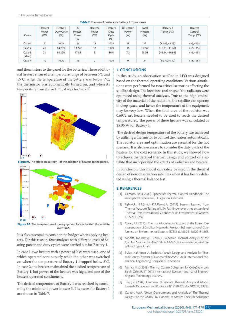
and thermistors to the panel for the batteries. These additio-nal heaters ensured a temperature range of between 5°C and 15°C: when the temperature of the battery was below 5°C, the thermistor was automatically turned on, and when its temperature rose above 15°C, it was turned off.

Figure 9. The effect on Battery 1 of the addition of heaters to the panels.

Figure 10. The temperature of the equipment located within the satellite over time.

It is also essential to consider the budget when applying hea-ters. For this reason, four analyses with different levels of he-ating power and duty cycles were carried out for Battery 1.

In case 1, two heaters with a power of 9 W were used, one of which operated continuously while the other was switched on when the temperature of Battery 1 dropped below 5°C. In case 2, the heaters maintained the desired temperature of Battery 1, but power of the heaters was high, and one of the heaters operated continously.

The desired temperature of Battery 1 was reached by consu-ming the minimum power in case 3. The cases for Battery 1 are shown in Table 7.

7. CONCLUSIONSIn this study, an observation satellite in LEO was designed based on the thermal operating conditions. Various simula-tions were performed for two critical scenarios affecting the satellite design. The locations and areas of the radiators were optimised using thermal analyses. Due to the high emissi-vity of the material of the radiators, the satellite can operate in deep space, and hence the temperature of the equipment may be very low. When the total area of the radiator was 0.6972 m2, heaters needed to be used to reach the desired temperatures. The power of these heaters was calculated as 25.06 W for Battery 1.

The desired design temperature of the battery was achieved by utilising a thermistor to control the heaters automatically. The radiator area and optimisation are essential for the hot scenario. It is also necessary to consider the duty cycle of the heaters for the cold scenario. In this study, we showed how to achieve the detailed thermal design and control of a sa-tellite that incorporated the effects of radiators and heaters.

In conclusion, this model can safely be used in the thermal design of new observation satellites when it has been valida-ted using a thermal balance test.

8. REFERENCES[1] Gilmore, D.G.( 2002). Spacecraft Thermal Control Handbook. The

Aerospace Corporation, El Segundo, California.

[2] Fishwick, N.A,Smith K.A,Perez.J.A. (2015). Lessons Learned from Thermal Vacuum Testing of LISA Pathfinder over three system level Thermal Tests.International Conference on Environmental Systems.ICES 2015-246.

[3] Coker, R.F. (2013). Thermal Modeling in Support of the Edison De-monstration of Smallsat Networks Project.43rd International Con-ference on Environmental Systems (ICES). doi:10.2514/6.2013-3368.

[4] Moffitt, B.A.,Batty,J.C. (2002). Predictive Thermal Analysis of the Combat Sentinel Satellite.16th AIAA/USU Conference on Small Sa-tellites, Logan, Utah.

[5] Bulut, .Kahriman, A, Sozbir,N. (2010). Design and Analysis for Ther-mal Control System of Nanosatellite.ASME 2010 International Me-chanical Engineering Congress & Exposition.

[6] Mishra, H.V. (2018). Thermal Control Subsystem for CubeSat in Low Earth Orbit.IRJET 2018 International Research Journal of Enginee-ring and Technology, 946-949.

[7] Tsai, J.R. (2004). Overview of Satellite Thermal Analytical Model. Journal of Spacecraft and Rockets, 41(1):120-125. doi:10.2514/1.9273.

[8] Garzon, M.M. (2012). Development and Analysis of The Thermal Design For the OSIRIC-3U Cubesat, A Master Thesis in Aerospace

Table 7. The use of heaters for Battery 1: Three cases

Cases

Heater1 Power

(W)

Heater1Duty Cycle

(%)

ƩHeater1 Power

(W)

Heater2 Power

(W)

Heater1DutyCycle (%)

Ʃ Heater2 Power

(W)

Total Heaters

(W)

Battery-1Temp. (°C)

HeatersControl

Temp. (°C)

Case-1 9 100% 9 18 100% 18 27 (+2.43,+5.15) (+5,+15)

Case-2 21 63.20% 13.272 18 100% 18 31.272 (+6.31,+11.38) (+5,+15)

Case-3(Ideal)

21 84.22% 17.86 9 80% 7.2 25.06 (+6.14,+10.91) (+5,+15)

Case-4 15 100% 15 9 100% 9 24 (+6.77,+9.19) (+5,+15)

178 European Mechanical Science (2020), 4(4): 171-178 doi: https://doi.org/10.26701/ems.730201

Detailed Thermal Design and Control of an Observation Satellite in Low Earth Orbit

Engineering,Penn State University.

[9] Hurman,J.L. (2012).Optimization of steady-state thermal design of space radiators. Journal of Spacecraft and Rockets 6:10. doi: 10.2514/3.29773

[10] Aslanturk, C. (2006). Optimization of a central-heating radiator. American Institute of Aeronautics and Astronautics. 6:10 doi: 10.2514/3.29773

[11] Doner, N. (2014). M1 Model for Radiative Heat Transfer in Absor-bing, Emitting, and Scattering Medium, International Journal of Thermal Sciences, Volume 79,34-39.

[12] Aksu,A.Sundu.H,Mermer,E. (2019) Nonlinear system identificati-on for the thermal management of communication satellites EU-CASS2019 doi:10.13009/ EUCASS2019-910

[13] Sharma, A.K. (2013). Surface Engineering For Thermal Control of Spacecraft. Journal Surface Engineering, 21(3): 249-253. do-i:10.1179/174329405X50118

[14] Thermica User’s Manual, Version 4.8.0.P1.

[15] Lauga, R.P. (2017). Using real Earth Albedo and Earth IR Flux for Spacecraft Thermal Analysis, 47th International Conference on En-vironmental Systems(ICES)-2017-142

[16] Vujičić, M. R., Lavery, N. P., & Brown, S. G. R. (2006). Numerical sen-sitivity and view factor calculation using the Monte Carlo method. Proceedings of the Institution of Mechanical Engineers, Part C: Jour-nal of Mechanical Engineering Science, 220(5), 697-702.

[17] Iucci, N., Dorman, L. I., Levitin, A. E., Belov, A. V., Eroshenko, E. A., Ptit-syna, N. G., & Tyasto, M. I. (2006). Spacecraft operational anomalies and space weather impact hazards. Advances in Space Research, 37(1), 184-190.