Detailed optical and nearinfrared polarimetry ... · and broad-band photometry of the afterglow of...

Mon. Not. R. Astron. Soc. 426, 2–22 (2012) doi:10.1111/j.1365-2966.2012.20943.x

Detailed optical and near-infrared polarimetry, spectroscopyand broad-band photometry of the afterglow of GRB 091018:polarization evolution

K. Wiersema,1� P. A. Curran,2 T. Kruhler,3 A. Melandri,4,5 E. Rol,6 R. L. C. Starling,1

N. R. Tanvir,1 A. J. van der Horst,6 S. Covino,4 J. P. U. Fynbo,3 P. Goldoni,7

J. Gorosabel,8 J. Hjorth,3 S. Klose,9 C. G. Mundell,5 P. T. O’Brien,1 E. Palazzi,10

R. A. M. J. Wijers,6 V. D’Elia,11,12 P. A. Evans,1 R. Filgas,13 A. Gomboc,14,15

J. Greiner,13 C. Guidorzi,16 L. Kaper,6 S. Kobayashi,5 C. Kouveliotou,17 A. J. Levan,18

A. Rossi,9 A. Rowlinson,1,6 I. A. Steele,5 A. de Ugarte Postigo3,8 and S. D. Vergani41University of Leicester, University Road, Leicester LE1 7RH2Laboratoire AIM, CEA/IRFU-Universite Paris Diderot-CNRS/INSU, CEA DSM/IRFU/SAp, Centre de Saclay, F-91191 Gif-sur-Yvette, France3Dark Cosmology Centre, Niels Bohr Institute, University of Copenhagen, Juliane Maries Vej 30, 2100 Copenhagen, Denmark4INAF – Osservatorio Astronomico di Brera, via E. Bianchi 46, I-23807 Merate, Italy5Astrophysics Research Institute, Liverpool John Moores University, Twelve Quays House, Egerton Wharf, Birkenhead CH41 1LD6Astronomical Institute ‘Anton Pannekoek’, University of Amsterdam, 1090 GE Amsterdam, the Netherlands7Laboratoire Astroparticule et Cosmologie, 10 rue A. Domon et L. Duquet, 75205 Paris Cedex 13, France8IAA – CSIC, Glorieta de la Astronomıa s/n, 18008 Granada, Spain9Thuringer Landessternwarte Tautenburg, Sternwarte 5, 07778 Tautenburg, Germany10INAF – Istituto di Astrofisica Spaziale e Fisica Cosmica di Bologna, Via Gobetti 101, I-40129 Bologna, Italy11INAF – Osservatorio Astronomico di Roma, via di Frascati 33, 00040 Monte Porzio Catone, Italy12ASI-Science Data Center, via Galileo Galilei, 00044 Frascati, Italy13Max-Planck-Institut fur Extraterrestrische Physik, Giessenbachstraße 1, 85748 Garching, Germany14Faculty of Mathematics and Physics, University of Ljubljana, Jadranska 19, SI-1000 Ljubljana, Slovenia15Centre of Excellence SPACE-SI, Askerceva cesta 12, SI-1000 Ljubljana, Slovenia16Physics Department, University of Ferrara, via Saragat 1, I-44122, Ferrara, Italy17Space Science Office, VP62, NASA/Marshall Space Flight Center Huntsville, AL 35812, USA18Department of Physics, University of Warwick, Coventry CV4 7AL

Accepted 2012 March 15. Received 2012 March 14; in original form 2012 February 10

ABSTRACTFollow-up observations of large numbers of gamma-ray burst (GRB) afterglows, facilitatedby the Swift satellite, have produced a large sample of spectral energy distributions andlight curves, from which their basic micro- and macro-physical parameters can in principle bederived. However, a number of phenomena have been observed that defy explanation by simpleversions of the standard fireball model, leading to a variety of new models. Polarimetry can bea major independent diagnostic of afterglow physics, probing the magnetic field properties andinternal structure of the GRB jets. In this paper we present the first high-quality multi-nightpolarimetric light curve of a Swift GRB afterglow, aimed at providing a well-calibrated dataset of a typical afterglow to serve as a benchmark system for modelling afterglow polarizationbehaviour. In particular, our data set of the afterglow of GRB 091018 (at redshift z = 0.971)comprises optical linear polarimetry (R band, 0.13–2.3 d after burst); circular polarimetry(R band) and near-infrared linear polarimetry (Ks band). We add to that high-quality opticaland near-infrared broad-band light curves and spectral energy distributions as well as afterglowspectroscopy. The linear polarization varies between 0 and 3 per cent, with both long and short

�E-mail: [email protected]

C© 2012 The AuthorsMonthly Notices of the Royal Astronomical Society C© 2012 RAS

at Leicester U

niversity Library on July 21, 2015

http://mnras.oxfordjournals.org/

Dow

nloaded from


Polarimetry of the afterglow of GRB 091018 3

time-scale variability visible. We find an achromatic break in the afterglow light curve, whichcorresponds to features in the polarimetric curve. We find that the data can be reproducedby jet break models only if an additional polarized component of unknown nature is presentin the polarimetric curve. We probe the ordered magnetic field component in the afterglowthrough our deep circular polarimetry, finding Pcirc < 0.15 per cent (2σ ), the deepest limit yetfor a GRB afterglow, suggesting ordered fields are weak, if at all present. Our simultaneousR- and Ks-band polarimetry shows that dust-induced polarization in the host galaxy is likelynegligible.

Key words: acceleration of particles – techniques: polarimetric – gamma-ray burst: individ-ual: GRB 091018.

1 I N T RO D U C T I O N

Collimated outflows in the form of jets are ubiquitous, from activegalactic nucleus jets driven by accretion of material by supermas-sive black holes in galactic centres to those associated with stellarsources such as X-ray binaries and galactic microquasars. A par-ticularly exciting view of the fundamental physics of jet sourcesis offered by gamma-ray bursts (GRBs), which form the extremeend of the energy and Lorentz factor parameter space. Since thediscovery of afterglows in 1997 (Costa et al. 1997; van Paradijset al. 1997) we have a broad picture of the origin and cause ofGRBs: through a catastrophic event (in the case of long-durationGRBs this is the core collapse of a massive star), a jet of highlyrelativistic material is ejected. In the standard fireball model (e.g.Meszaros & Rees 1997), the resulting broad-band emission de-tected from X-ray energies through to radio waves – the so-calledafterglow – is explained by the relativistic ejecta colliding withthe surrounding circumburst medium. The afterglow radiation wedetect is consistent with a synchrotron emission (e.g. Meszaros &Rees 1992, 1997; Wijers & Galama 1999), characterized by a se-ries of smoothly connected power laws, with characteristic breakfrequencies and fluxes. The macroscopic properties of shocks arelargely understood, and the dynamics of the shock created whenthe relativistic jet hits the circumstellar matter can be written downin terms of the explosion energy, the density (and density gradient)of the medium into which the shock ploughs and the compositionof the shocked material. However, outstanding questions remainon the nature of the microphysics: how are the relativistic parti-cles that radiate the observed emission accelerated? Where doesthe magnetic field in the shocked region come from and what is itsstructure?

Since its launch in 2004, the Swift satellite (Gehrels et al.2004) has provided us with hundreds of well-sampled X-ray andUV/optical afterglow light curves from seconds to months after burst(see Gehrels, Ramirez-Ruiz & Fox 2009 for a review). These lightcurves revealed complexity that was unexpected from pre-Swift lightcurves (Piran & Fan 2007); the standard fireball model has receiveda growing number of modifications, and the concept of a canonicallight curve was introduced to explain the steep fades, plateau phasesand multiple breaks in Swift X-ray light curves (Nousek et al. 2006).In particular, discrepancies between X-ray and optical light curvesof GRB afterglows and the rich array of light curve morphologyincluding extended plateaux, rebrightenings and flares challengeexisting GRB models (see Piran & Fan 2007 for a review). Ex-planations for these features include complex jet structure, energyre-injection due to late-time central energy activity, variable micro-physics and off-axis emission, with a combination of effects likely

in action in most afterglows. However, these model variations are inprinciple non-degenerate: linear and circular polarimetry have theability to separate out the various models for the behaviour of the(early) afterglows in a completely independent way, as these modelshave different implications for the magnitude and orientation of theoptical polarization, as well as for their time dependence (e.g. Rossiet al. 2004).

The ground-breaking discovery and interpretation of suddenachromatic steepening in light curves at ∼1d post-burst in pre-Swift GRBs – so-called jet breaks – provided the first convincingevidence of highly collimated ejection (e.g. Rhoads 1997, 1999;Sari, Piran & Halpern 1999) and allowed jet opening angles andcollimation-corrected energies to be derived (e.g. Frail et al. 2001).Jet breaks were expected to be ubiquitous in Swift light curves, butthe added complexity and multiple breaks in these light curves havemade jet breaks difficult to identify unambiguously (e.g. Curranet al. 2007a). In contrast, the linear polarization around the time ofthe jet break is predicted to have a unique signature (Ghisellini &Lazzati 1999; Sari 1999; Rossi et al. 2004): at early times a distantobserver located slightly off-axis will see the afterglow as a ring-shaped source, which has strong polarization in the radial direction(assuming that the magnetic field is compressed in the plane nor-mal to the motion, i.e. ordered in the plane of the shock). In thereceived light, integrated over the ring, the polarization will largelycancel out. However, as the fireball decelerates the size of the ringincreases and at some point the edge of the jet is reached, at whichpoint the polarization does not completely cancel out anymore andlinear polarization is observed. As the ring expands further, the op-posite edge of the jet is reached as well, giving rise to a secondpeak in the linear polarization curve. Therefore polarimetry pro-vides a useful tool to unambiguously identify jet breaks from otherlight curve breaks, though measured polarization curves of GRBafterglows have in some cases shown puzzling features (see e.g.the cases of GRBs 030329 and 020405 discussed further in Section4.1). In addition, the linear polarization properties probe jet inter-nal structure, as different polarization properties are predicted for‘uniform’ or ‘structured’ jet energy distributions (Rossi et al. 2004,see also Section 4.2.2).

It has been shown that if some fraction of the magnetic field inthe shock has large-scale order, the light may also be circularlypolarized (Matsumiya & Ioka 2003; Sagiv, Waxman & Loeb 2004).For the forward shock (in the ambient medium), most models pre-dict 0.01–1 per cent circular polarization during the first day (e.g.Matsumiya & Ioka 2003), depending on the strength and order ofthe magnetic fields and the wavelength of observation. Part of thisrange is within reach of large telescopes, as we will demonstrate inSection 3.2.

C© 2012 The Authors, MNRAS 426, 2–22Monthly Notices of the Royal Astronomical Society C© 2012 RAS

at Leicester U



Dow

nloaded from


4 K. Wiersema et al.

In the Swift era few polarimetric measurements have been per-formed. Arguably the most successful have been the early-time lin-ear polarization measurements of the afterglows of GRBs 060418and 090102, performed with the RINGO polarimeter on the rapidlyresponding robotic Liverpool Telescope (Mundell et al. 2007; Steeleet al. 2009), the latter GRB showing a linear polarization of 10 percent just 190 s after burst. Steele et al. (2009) interpret the light curveproperties and high degree of polarization in GRB 090102 – whichwas detected when emission from the reverse shock dominated thereceived optical light – as evidence for large-scale ordered magneticfields in the expanding fireball. This detection of significant polar-ization at early times provides strong motivation for following thepolarization properties of the fading afterglow for many hours ordays after the GRB. However, late-time polarimetric observationsof GRBs (see Lazzati 2006 for an overview) show that the combi-nation of fading afterglow and low levels of polarization (few percent) requires large telescopes to obtain polarimetric observationsover multiple days to high precision (�0.3 per cent), using multiplefilters to distinguish dust induced from intrinsic afterglow polariza-tion. In this paper we present the first such data set for a Swift burst,and the most extensive polarimetric data set of any burst since GRB030329 (Greiner et al. 2003).

This paper is the first in a series on the afterglow of GRB 091018.In this first paper we will describe our data set in detail and comparethe observed polarization light curves with those of other (pre-Swift) bursts and theoretical models. In a forthcoming second paper(Wiersema et al. in preparation; hereafter called Paper 2) we willdiscuss the dust properties in GRB sightlines from a combinationof multi-wavelength polarimetry, spectroscopy, host imaging andbroad-band afterglow spectral energy distributions. In a third paper(Paper 3) we will model the afterglow physics of GRB 091018 ingreater detail and fit the polarization data to more detailed models,in particular considering energy injection.

This paper is organized as follows: in Section 2 we describethe polarimetry, spectroscopy and broad-band photometry observa-tions, the data reduction and data calibration techniques; in Sec-tion 3 we discuss the detected features in the data and in Section 4we compare the data to models and previous studies of afterglowpolarimetric light curves. Throughout this paper we adopt a cos-mology with H0 = 71 km s−1 Mpc−1, �m = 0.27, �� = 0.73.

2 OBSERVATIONS

GRB 091018 triggered the Burst Alert Telescope (BAT) on board theSwift satellite at 20:48:19 UT on 2009 October 18 (trigger 373172;Stamatikos et al. 2009). The prompt emission shows the burst tolikely belong to the class of long bursts (Kouveliotou et al. 1993),with a duration of T90 = 4.4 ± 0.6 s (Markwardt et al. 2009; Ukwattaet al. 2012 report a spectral lag of 143 ± 297 ms). An X-ray andoptical afterglow were found by the SwiftX-Ray Telescope (XRT)and UV–Optical Telescope (UVOT). Chen et al. (2009) reportedan afterglow redshift of 0.971 shortly after. Based on the initialbrightness of the UVOT afterglow we activated our Very LargeTelescope (VLT) polarimetry programme (programme 084.D-0949,PI: Wiersema).

2.1 R-band linear and circular polarimetry

2.1.1 Data acquisition

We acquired imaging polarimetry using the Focal Reducer and lowdispersion Spectrograph (FORS2) mounted on Unit Telescope 1

Figure 1. Small sections of data frames from the Infrared Spectrometerand Array Camera (ISAAC) Ks-band polarimetry (Left; angle 0 frame fromlinK1, see Section 2.2) and optical FORS2 polarimetry (right; angle −45from circular polarimetry epoch cir1). The circles are 5 arcsec in radius ineach image and show the source in the o and e beams.

(Antu) of the VLT, using the FORS2 Rspecial filter. After passingthrough a half or quarter wavelength plate (in the case of linearand circular polarimetry, respectively), a Wollaston prism splits theincoming light into an ordinary and extraordinary beam (hereafterthe o and e beams) that are perpendicularly polarized. These oand e beams are imaged simultaneously, using a mask to avoidoverlap of the two beams on the chip, as shown in Fig. 1. Foreach linear polarization data set we used four rotation angles ofthe half wavelength plate of 0, 22.5, 45 and 67.◦5. The circularpolarization data were taken with −45◦ and +45◦ angles of thequarter wavelength plate.

To ensure relatively homogeneous polarimetric uncertainties as afunction of time, exposure time was increased as the source faded.We employed a small dithering pattern, while taking care not to po-sition the afterglow too close to the edges of the mask. We acquireda total of 20 linear polarization series and four circular polarizationseries, see Table 1.

We began our FORS2 polarimetric monitoring with a single shortsequence of linear polarimetry. After this, to make full use of thebrightness of the afterglow we switched to circular polarimetry,for which the models predict a much lower degree of polarization,requiring a large number of detected photons. Directly followingthe circular polarization, we continued our linear polarimetry. Weobtained a further six sequences, and a further two at the end of thenight. The next night we obtained further data sets at the beginningand the end of the night. A last, deep, point was obtained in the thirdnight. Note that for all FORS2 polarimetry we position the afterglowclose to the centre of the FORS2 field of view, on chip 1, whereinstrumental polarization is very low (well below our statisticalerrors, Patat & Romaniello 2006).

2.1.2 Data reduction and calibration

We bias and flat field corrected all data using tasks in IRAF and usingstandard twilight sky flats. We use our own software in combinationwith IRAF routines to perform aperture photometry on the o and eimages of the afterglow to find the source fluxes f o and f e, using thesame approach as Rol et al. (2003). We used a seeing matched aper-ture of 1.5 times the on-frame full width at half-maximum (FWHM)of the point spread function (PSF), fitted per frame independentlyfor the o and e as small differences in PSF shape may occur betweenthe o and e beams, particularly for objects far off-axis. The sky sub-traction was done using an annulus of inner and outer radii threeand four times the FWHM. We measure f o and f e for all point-likeobjects in all frames.

We express the polarimetry information in terms of the Stokesvector S = (Q, U, V , I ) (see e.g. Chandrasekhar 1960), wherethe components of this vector have the following meaning: Q andU contain the behaviour of the linear polarization; V the circu-lar polarization and I is the intensity. Generally we will use the


at Leicester U



Dow

nloaded from



Table 1. Log of our polarimetric observations. The ID column gives a label to each polarimetric data set tomake discussion easier, with linear polarimetry data sets labelled ‘lin’ and circular polarimetry ‘cir’. Theexposure time is the exposure time per retarder angle (four angles for linear, two for circular polarimetry).The Q/I and U/I values are as measured: to obtain values corrected for scattering on Galactic dust, subtractthe values derived in Section 2.1.3.

FORS2, Rspecial

ID T − T0 Exposure time Q/I U/I V/I(mid; d) (s)

lin1 0.131 89 180.0 −0.0014 ± 0.0009 −0.0036 ± 0.0009cir1 0.143 02 300.0 −0.0005 ± 0.0014cir2 0.151 33 300.0 0.0011 ± 0.0015cir3 0.159 64 300.0 0.0003 ± 0.0015cir4 0.167 95 300.0 −0.0017 ± 0.0015lin2 0.180 43 240.0 0.0009 ± 0.0009 −0.0040 ± 0.0009lin3 0.197 01 300.0 −0.0012 ± 0.0008 0.0024 ± 0.0008lin4 0.212 82 300.0 0.0010 ± 0.0009 −0.0023 ± 0.0009lin5 0.230 30 300.0 −0.0006 ± 0.0009 −0.0037 ± 0.0009lin6 0.246 11 300.0 0.0083 ± 0.0009 −0.0039 ± 0.0009lin7 0.263 57 300.0 0.0056 ± 0.0009 −0.0025 ± 0.0009lin8 0.279 36 300.0 0.0057 ± 0.0009 −0.0063 ± 0.0009lin9 0.454 83 300.0 0.0119 ± 0.0012 −0.0025 ± 0.0012lin10 0.470 64 300.0 0.0067 ± 0.0012 −0.0009 ± 0.0012lin11 1.139 40 300.0 −0.0162 ± 0.0023 0.0078 ± 0.0023lin12 1.155 22 300.0 −0.0167 ± 0.0022 0.0260 ± 0.0023lin13 1.173 45 300.0 0.0088 ± 0.0023 0.0130 ± 0.0023lin14 1.189 26 300.0 −0.0123 ± 0.0023 −0.0147 ± 0.0023lin15 1.207 29 300.0 −0.0070 ± 0.0024 −0.0054 ± 0.0024lin16 1.223 10 300.0 −0.0126 ± 0.0024 −0.0080 ± 0.0024lin17 1.360 06 600.0 0.0022 ± 0.0018 −0.0056 ± 0.0018lin18 1.391 83 600.0 0.0014 ± 0.0018 0.0057 ± 0.0019lin19 1.449 26 600.0 −0.0141 ± 0.0019 −0.0031 ± 0.0019lin20 2.390 23 720.0 0.0111 ± 0.0023 −0.0092 ± 0.0023

ISAAC, Ks

linK∗ 0.4309 720.0a 0.0204 ± 0.0078 0.0008 ± 0.0083

aCombined value of three complete series (see Section 2.2).

normalized Stokes parameters q = Q/I, u = U/I and v = V/I inthis paper. Theoretical models are often expressed in terms of thepolarization degree P and polarization angle θ . These quantities canbe found from the Stokes parameters through the relations

Plin =√

Q2 + U 2

I

θ = 1

2arctan(U/Q) + φ

Pcir = V /I .

Constant φ is an offset defined so that the resulting angle θ conformsto the standard definitions of position angle (angle from north,counterclockwise, see Fig. 2):

φ =

⎧⎪⎪⎨⎪⎪⎩

0◦ if Q > 0 and U ≥ 0;

180◦ if Q > 0 and U < 0;

90◦ if Q < 0.

Note that the conversion from Stokes parameters to P brings withit complications, discussed further below, so wherever possible wewill work in Stokes parameter space.

To measure the Stokes Q/I and U/I parameters a measurementat two rotation angles suffices, but this introduces substantial sys-tematic uncertainties, caused by imperfect flat fielding, imperfect

Figure 2. Coordinate definitions used in this paper.

background subtraction and imperfect behaviour of the half wave-length plate and Wollaston prism. Using four rotation angles with aconstant stepsize (in this case of 22.◦5) means that several of thesesystematic effects cancel out (in particular the effects of backgroundsubtraction and flat fielding), leading to greatly improved polarimet-ric error terms. With these angles one can write (Patat & Romaniello


at Leicester U



Dow

nloaded from



2006)

q = Q/I = 2

N

N−1∑i=0

Fi cos (iπ/2) and

u = U/I = 2

N

N−1∑i=0

Fi sin (iπ/2) ,

where N is the number of half wavelength plate positions, and Fi isthe normalized flux difference of a source in the o and e beams atthe ith angle,

F i = (fo,i − fe,i

)/(fo,i + fe,i

) = (fo,i − fe,i

)/I .

For the circular polarimetry, taken with two angles of the retarder,we can simply write

v = V /I = 1

2(F45 − F−45) .

After measurement of the fluxes of the sources in the images wecompute their observed Stokes parameters and their uncertaintiesusing the expressions above. The afterglow is always positionedon nearly the same position on CHIP1 (barring a small dither of∼16 pixels in the Y direction in some epochs), on the optical axis.As such we expect the instrumental linear polarization to be negli-gible; see Patat & Romaniello (2006) for a thorough error analysisof FORS1, whose polarimetry optics were moved to the FORS2instrument in 2009. Additionally, circular polarimetry Stokes V/Ihas no instrumental polarization on axis. In conclusion, the valuesof the Stokes parameters found through the methods above allowan investigation of the time dependence of the afterglow q, u and v.

Theoretical models are generally expressed in terms of the linearand circular polarization fractions Plin and Pcir, and we thereforeconvert the Stokes parameter information to these quantities usingthe equations above. We note that the uncertainty on the linearpolarization angle is a function of the intrinsic polarization degree(σθ = σPlin/2Plin), which means that for the low polarization valuesand faint fluxes of afterglows the uncertainties in θ are very large.Finally, the position angles found are corrected for the instrumentalzero angle offset, which is −1.◦48 at 655 nm (the central wavelengthof the filter).1

Errors on q and u are generally distributed as a Normal distri-bution and the Stokes parameters can have positive and negativevalues. In contrast, Plin is a positive definite quantity. As demon-strated in Simmons & Stewart (1985) (their Section 2), integratingthe equation for the distribution of measured (P, θ ) over θ shows thatPlin follows a Rice probability distribution rather than a Gaussianone. Directly using the equations above will lead to overestimatedPlin and incorrect confidence intervals, an effect generally referredto as the linear polarization bias. The correction to the resulting Plin

and associated confidence ranges has been studied through bothanalytical and numerical (Monte Carlo) methods. Generally speak-ing, this correction depends on σ P, P and the signal-to-noise ratio(SNR) of f e + f o (i.e. the SNR of Ii). In the literature one often seesthe Wardle & Kronberg (1974) prescription used, in which the inputP values are multiplied by

√1 − (σP /P )2 to find the bias-corrected

polarization. We follow Sparks & Axon (1999) in using a parameterη = P × SNRF to trace the expected behaviour of the bias and σ P:when η > 2 the Wardle & Kronberg correction is valid, and σ P isas computed directly from the uncertainty of F. In our FORS2 dataset before correction for Galactic polarization (Section 2.1.3) all

1 Tabulated at the FORS instrument webpages.

data points have η > 2, and the bias correction is in all cases smallcompared to σ P.

2.1.3 Polarization induced by the Galactic interstellar medium

To bring the afterglow q and u to an absolute frame, we need tocorrect for the linear polarization induced by scattering on dust inour Galaxy (Galactic interstellar polarization, GIP). Note that V/Idoes not require a correction as there is no circular GIP and theresulting linear polarization is much smaller than the threshold fornoticeable linear–circular crosstalk (Patat & Romaniello 2006).

We assume here that the average intrinsic polarization of a suf-ficiently large sample of field stars is zero, that the bulk of thepolarizing dust is between these stars and the observer and thattherefore the observed distribution of q and u of field sources mea-sures the GIP. We measure the Stokes q and u values of all sourcesthat have an SNR above 20 in the FORS2 field, on both chips andin all epochs. A large number of artefacts are visible in our FORS2imaging polarimetry, which have the appearance of a group of stars,and which are likely caused by reflections at the retarder plate;2 wetake special care to avoid stars close to these artefacts.

We then eliminate sources that appear significantly extended(galaxies), which may give spurious linear polarimetric signals ifseeing conditions change during a polarimetric sequence. We fur-ther eliminate sources that are close to the mask edges and sourcesthat are close to saturation in one or more of the images.

It is well known that FORS1, whose polarimetric optics are nowcannibalized in FORS2, displayed a roughly radial instrumentallinear polarization pattern, with polarization magnitude dependingon the radial distance to the optical axis (see Patat & Romaniello2006). The shape of the linear polarization pattern and its mag-nitude depend on the wavelength, and was found to reach nearly∼1.5 per cent at the edges of the field of view (Patat & Romaniello2006). While this effect is well calibrated for FORS1 in the V and Ibands, a similar analysis has not yet been performed for FORS2. Wetherefore use a conservative approach and choose only stars close(radially) to the GRB position. It is of some importance to select notonly the brightest stars (which would give smallest uncertainty inthe GIP value), as this may result in a bias towards the nearest stars(in distance), and therefore may not sample the complete Galacticdust column towards the GRB. We also make sure that stars areselected with a fairly uniform distribution over the field (in termsof position angle).

We determine the GIP q and u values using three methods: wefind the weighted mean of the field star distribution; we fit one-dimensional Gaussian curves on the histograms of the q and udistributions and we fit a two-dimensional Gaussian function (withits orientation as a free parameter) on the (q, u) distribution afterconverting this to a two-dimensional histogram (where a range ofbin sizes are used based on the number of input data points). Weperform these fits for a range of limit values on the maximum radialdistance r between the input stars and the GRB, and on the maxi-mum allowed σ P of the stars. Unfortunately there are only a smallnumber of fairly bright stars near to the GRB position, making itnecessary to use a large limit on the radial distance to obtain a suf-ficient number of data points. We find a best balance between thenumber of sources in the fit and the uncertainties on the resultingqGIP and uGIP for limits σ P � 0.35 per cent and r � 2.0 arcmin (103

2 http://www.eso.org/observing/dfo/quality/FORS2/qc/problems/problems_fors2.html


at Leicester U



Dow

nloaded from



Figure 3. Measurements of q and u of field stars to determine the contribu-tion to the received polarization by scattering on dust within our Galaxy. Thedashed lines indicate q = 0 and u = 0. Binsize used in this plot is 0.0025.

data points). Note that r = 2 arcmin would correspond to ∼0.23and ∼0.34 per cent instrumental polarization in the V and I bandsin FORS1, respectively (Patat & Romaniello 2006). Using theselimits the three methods give very similar GIP values. In Fig. 3 thedistribution of data points (103 points) is shown. We find qGIP =−0.0028 and uGIP = −0.0036, or PGIP = 0.45 per cent, θGIP = 116◦.The two-dimensional fit gives the width of the Gaussian along theq axis as σ q = 0.0030 and along the u axis as σ u = 0.0025, andthe rotation of the containment ellipse from the q axis in radians,counter-clockwise, as = 1.7 rad. The evidence for deviation fromradial symmetry is not very strong, but the analysis of Patat &Romaniello (2006) shows that the FORS1 off-axis polarization pat-tern exhibited non-radial behaviour in the B band. We use this ellipseas a conservative error in the GIP Stokes parameters, following Rolet al. (2003). The fairly large uncertainty in these is likely domi-nated by the contribution of the unknown instrumental polarizationpattern and the low number of bright stars within ∼1 arcmin of theGRB position.

The empirical relation PGIP � 0.09E(B − V) (Serkowski,Matheson & Ford 1975) gives PGIP ∼ 0.3 per cent, which compareswell with the value derived above.

We now subtract from the GRB q and u values the qGIP and uGIP

found above, to remove the (constant in time) component to thepolarization caused by the Galactic interstellar medium (ISM). Wepropagate the errors on the GIP Stokes parameters into the resultingcorrected values qGIPcorr and uGIPcorr. As is clear from Table 1, theafterglow polarization at very early times (e.g. lin1, lin3) all butvanishes, indicating that at early times the detected polarization isdominated by GIP. In many epochs, the qGIPcorr and uGIPcorr errorsare dominated by the uncertainties in the GIP Stokes parameters.We compute GIP-corrected values for the polarization and positionangle, which will bring the measured values on to an absolute scale.It is clear that the errors σ P are increased dramatically, while Pdecreases in several epochs (to near zero in e.g. lin1), i.e. a drop in

Table 2. Linear polarization values, where coordinate definitions areused as in Fig. 2. All values have been corrected for polarization bias(after correction for GIP in the case of the last two columns), see Sec-tion 2.1.3. The uncertainties in the GIP q, u value are fully propagatedand dominate the uncertainties in the GRB afterglow GIP-corrected q,u. The GIP-corrected polarization is very low (with inferred values ofzero in two cases), and as such the errors on θ are very large (as σ θ is afunction of 1/P, see Section 2.1.2).

ID Plin θ Plin,GIPcorr θGIPcorr

(per cent) (degrees) (per cent) (degrees)

lin1 0.36 ± 0.13 126.1 ± 19.3 0 (0.32)b

lin2 0.38 ± 0.12 143.1 ± 17.7 0.21 ± 0.31 177.0 ± 47.5lin3 0.24 ± 0.11 60.2 ± 25.1 0.56 ± 0.27 37.7 ± 24.7lin4 0.22 ± 0.12 148.5 ± 28.4 0.26 ± 0.31 9.2 ± 43.7lin5 0.35 ± 0.12 132.1 ± 19.0 0 (0.32)b

lin6 0.90 ± 0.12 168.9 ± 7.9 1.07 ± 0.30 179.2 ± 16.1lin7 0.59 ± 0.12 169.5 ± 12.0 0.78 ± 0.31 3.9 ± 21.2lin8 0.84 ± 0.13 157.4 ± 8.8 0.84 ± 0.30 171.1 ± 19.9lin9 1.20 ± 0.17 175.5 ± 8.1 1.44 ± 0.32 2.2 ± 12.6lin10 0.65 ± 0.17 177.7 ± 14.7 0.94 ± 0.32 8.0 ± 18.6lin11 1.77 ± 0.32 78.6 ± 10.2 1.73 ± 0.36 69.8 ± 11.7lin12 3.07 ± 0.32 62.8 ± 5.9 3.25 ± 0.35 57.6 ± 6.1lin13 1.53 ± 0.32 29.5 ± 11.9 1.99 ± 0.35 27.6 ± 10.0lin14 1.89 ± 0.32 116.4 ± 9.8 1.42 ± 0.36 114.6 ± 14.0lin15 0.81 ± 0.33 110.2 ± 21.7 0.27 ± 0.38 101.6 ± 47.1lin16 1.45 ± 0.33 107.7 ± 13.0 1.00 ± 0.38 102.2 ± 20.2lin17 0.54 ± 0.25 147.0 ± 24.0 0.41 ± 0.34 168.8 ± 36.6lin18 0.52 ± 0.26 39.5 ± 25.3 0.97 ± 0.32 32.8 ± 17.8lin19 1.42 ± 0.27 97.6 ± 10.7 1.08 ± 0.35 88.7 ± 17.9lin20 1.40 ± 0.32 161.6 ± 13.1 1.45 ± 0.37 169.0 ± 14.3

linKa 2.0 ± 0.8 10.9 ± 20.9 2.0 ± 0.8 10.9 ± 20.9

aCombined value from linK1, linK2 and linK3. The GIP correction in theK band is more than an order of magnitude smaller than the statisticalerror in the polarization, so no correction is made. bSee Simmons &Stewart (1985) for the probability of correctly inferring true polarizationp0 = 0 from measured polarizations P using a maximum likelihoodestimator. The number in parentheses is the 67 per cent confidenceinterval boundary.

P/σ P. At the same time, the statistical detection signal to noise (i.e.SNR of Ii, simply referred to as SNR in Section 2.1.2) stays thesame. As the polarization bias is a function of both SNR and P/σ P,the polarization bias correction is much larger in several epochsafter GIP correction, showing the necessity of treating GIP effectsin q, u space rather than P, θ space in low polarization regimes. Inseveral cases the Wardle & Kronberg prescription is not valid (seeSimmons & Stewart 1985), and we use the methods recommendedby Simmons & Stewart (1985) for low P/σ P situations (which usea maximum likelihood estimator; this estimator has the lowest biasfactor and lowest risk function values in this signal-to-noise range).In two cases this led to robust zero polarization values. We refer toSimmons & Stewart (1985) for a discussion on the probability ofcorrectly inferring zero polarization for different estimators.

All resulting values are listed in Table 2.

2.2 K-band linear polarimetry

2.2.1 Data acquisition

We obtained an imaging polarimetry data set using the short-wavepolarization (SWP) mode of the ISAAC instrument mounted onUnit Telescope 3 (Melipal) of the VLT, using the Ks filter. Observa-tions coincided in part with R-band linear polarimetry, see Table 1.


at Leicester U



Dow

nloaded from



ISAAC SWP mode uses a similar approach to FORS2 to obtainpolarimetry: a Wollaston prism is inserted in the light path, and theincoming light is split into an ordinary and extraordinary beam (theo and e beam) that are perpendicularly polarized. The o and e beamsare imaged simultaneously, using a mask to avoid overlap. The an-gular separation of the o and e images is wavelength dependent. Themain difference between ISAAC and FORS2 imaging polarimetryis that a half wavelength plate is not present in ISAAC, requiringrotation of the instrument to obtain observations at the necessaryangles, and the location of ISAAC in the Nasmyth focus.

At each instrument angle we use integration times of 4 ×15 s, executed four times with significant dithering to facilitatesky subtraction. Because of the aperture mask, less than half of thefield of view is visible at any given rotation angle, and one generallyuses a dither pattern designed to sample the entire field. However,as the afterglow is faint and polarization low, we dither such thatthe afterglow always stays within the mask opening. After these4 × 60 s exposures, the instrument is rotated, and observations arerepeated for the new position angle. By mistake we employed cu-mulative rotation offsets of 0, 22.5, 22.5 and 22.◦5. As ISAAC doesnot have a half wavelength plate, the better choice of cumulative an-gles would have been 0, 45, 45, 45, so as to achieve the same effectsas in the FORS data (switching of the o and e images to minimizeflat-field errors and Wollaston throughput uncertainties). These se-ries of observations are repeated three times, resulting in completesets linK1, linK2 and linK3. Note that because of the rotation ofthe instrument, field stars are only visible in some of the rotationangles and rotate behind the mask at other angles. We note that aseries of data were taken before linK1 with an erroneous dither-ing pattern: the afterglow disappeared behind the aperture mask atthe third and fourth angle. In further analysis we will only use thecomplete cycles linK1–linK3: the calibration as described belowrequires measurement of both q and u for a given parallactic angle.

2.2.2 Data reduction and calibration

Data were corrected for dark current, flat fielded and backgroundsubtracted using tasks in IRAF, and the four exposures of 60 s perangle per cycle were co-added. Aperture photometry was performedon the e and o images of the afterglow, in the same way as describedabove for FORS2. We compute the normalized Stokes parameters:

q = Q/I = (Io,0 − Ie,0)

(Io,0 + Ie,0)and u = U/I = (Io,45 − Ie,45)

(Io,45 + Ie,45),

using the data with rotation angles 0 and 45◦. As we did not takedata with 90◦ and 135◦ angles, we cannot use these to cancel outsystematics as we did with the FORS2 data. We expect these effectsto be of the same order or smaller as the statistical errors (theafterglow was faint in K). We also compute Stokes parameters fromthe 22.◦5 and 67.◦5 data:

q2 = (Q/I )2 = (Io,22.5 − Ie,22.5)

(Io,22.5 + Ie,22.5)and

u2 = (U/I )2 = (Io,67.5 − Ie,67.5)

(Io,67.5 + Ie,67.5),

which we will calibrate independently [they differ from (q, u) by arotation in coordinate basis].

ISAAC is a Nasmyth focus instrument, and as such less wellsuited to accurate polarimetry: the instrumental polarization of Nas-myth instruments is dominated by reflection of the tertiary mirrorM3 (at 45◦, therefore introducing strong polarization which is highly

dependent on position or parallactic angle), which requires partic-ular care in calibration. Our calibration strategy closely follows therecommendations of Joos et al. (2008) and Witzel et al. (2011).These authors highlight in their papers the great benefits of usinga train of Mueller matrices to create a polarimetric model of theinstrument plus telescope for Nasmyth mounted instruments: allelements contributing to instrumental polarization effects are de-scribed in 4 × 4 matrices acting on the Stokes vector S. Thesematrices are then multiplied to give a Mueller matrix of the wholetelescope/instrument for a given wavelength and a given set-up. Werefer to Joos et al. (2008) for a detailed breakdown of the requiredmatrix components. The Mueller matrix M(θ , λ) describing the ef-fects of the M3 mirror on the polarization is a function of the lightincident angle θ , wavelength λ and the refraction index componentsn and k of the reflecting surface of M3. For these latter values weuse the values at the K band as derived by Witzel et al. (2011).

We obtained observations of the unpolarized DA white dwarf GJ915 (WD 2359−434; Fossati et al. 2007) using the same instrumentrotation angles as the science data and at a similar parallactic angle(60◦ at mid of the observation versus 50◦ for the mid of the range ofthe science series). Our calibrator observations were obtained justbefore the ISAAC science observations. We add to these observa-tions from the European Southern Observatory (ESO) data archiveof unpolarized white dwarf WD 1620−391 (using identical rotatorangles as our data), taken on 2009 September 16, with parallacticangle 76◦. Using these stars and the Mueller matrices describedabove we calibrate our Stokes parameters. Using our own standardstar observations and those of 2008 gave consistent results withinthe errors. Because of the way we dithered our data and the lownumber of bright field stars, we cannot refine our calibration usingfield stars. We then rotate the (q2, u2) values to the same orientationas (q, u). Because the source was fairly faint in the Ks band, the er-rors on the Stokes parameters of linK1-3 are large, and we thereforecombine them together, finding a combined q = 0.0204 ± 0.0078and u = 0.000 81 ± 0.0083.

There are no field stars available for an independent GIP cali-bration in the Ks band, but we can estimate the likely contributionof GIP to the observed values by using the approximate relationp(λ) ∝ λ−1.8 (see Martin & Whittet 1990). While the value of theexponent has fairly large uncertainty, it is clear that a GIP in theR band of ∼0.45 per cent corresponds to an expected GIP contri-bution in the Ks band of <0.1 per cent, i.e. an order of magnitudesmaller than the statistical uncertainties in the value above. We there-fore make no correction to the Ks-band Stokes parameters above.Using the same techniques as for the FORS2 data we compute abias-corrected linear polarization in the Ks band of 2.0 ± 0.8 percent with a position angle of 10.9 ± 20.◦9.

2.3 X-shooter spectroscopy

After the discovery of an optical afterglow, we activated our VLTX-shooter (mounted on UT2 of the VLT, Kueyen) programmefor GRB afterglow spectroscopy (programme ID 084.A-0260, PI:Fynbo). We obtained 4 × 600 s exposures with midpoint 0.1485 d(1.283 × 104 s) after burst. X-shooter is an echelle spectrograph withthree arms, the UVB, VIS and NIR arms, separated by dichroics,resulting in a wavelength coverage ∼0.3–2.4 µm. We used a 1 ×2 binning in the UVB and VIS arms (binning in the wavelengthcoordinate). A 5 arcsec nod throw was used to facilitate accuratesky subtraction, particularly important in the NIR arm, resulting inexposures taken in an ABBA pattern. We processed the data using


at Leicester U



Dow

nloaded from



version 1.3.0 of the ESO X-shooter data reduction pipeline (Goldoniet al. 2006), using the so-called physical mode.

Flux calibration is achieved using exposures of the flux standardstar BD+17 4708. Telluric line correction of the NIR arm spec-trum was performed using methods outlined in Wiersema (2011)with the SPEXTOOL software (Cushing, Vacca & Rayner 2004), usingobservations of the B9V star HD 16226. The resulting spectra arenormalized.

2.4 Optical and near-infrared photometry

2.4.1 GROND afterglow photometry

The seven-channel Gamma-Ray Burst Optical and Near-InfraredDetector (GROND; Greiner et al. 2008) mounted on the ESO 2.2 mtelescope observed the field of GRB 091018 using the g′, r′, i′, z′, J,H, Ks filters beginning as soon as the source became visible fromLa Silla observatory (Filgas et al. 2009). Photometric calibrationwas achieved through observations of photometric standard starfields. A spectral energy distribution using some of the GRONDdata presented here was published earlier in Greiner et al. (2011).

2.4.2 Faulkes Telescope South afterglow photometry

We observed the optical afterglow using the Faulkes TelescopeSouth (FTS), at Siding Spring, Australia. Observations were per-formed at two different epochs (about 15.3 h and 3.7 d after theburst event), using the R and i filters. These observations are com-plementary to those of GROND, filling the gap in coverage duringdaytime in Chile. All the images were cross-calibrated using theGROND field star measurement.

2.4.3 VLT afterglow photometry

As part of our linear and circular polarization monitoring cam-paign described above, a large series of acquisition images weretaken for accurate positioning of the afterglow within the aperturemask. Within each of these images the afterglow is detected at goodsignal-to-noise levels. We reduce the 14 FORS2 and two ISAAC ac-quisition images using flat fields, dark and bias fields taken the samenight. The FORS2 acquisition data were taken using the Rspecial fil-ter, and the ISAAC data using the Ks filter. We use a sample of fieldstars in the GROND data to bring the FORS2 acquisition photom-etry to the same homogeneous calibration. The ISAAC data werecalibrated using four 2MASS stars in the field of view. The resultingmagnitudes were converted to AB magnitudes; the resulting valuesare reported in Table 3.

In addition to the polarimetry acquisition images, we also pho-tometer the acquisition image taken for the X-shooter spectroscopy,calibrating on to the GROND system.

2.4.4 Gemini-South afterglow and host photometry

We followed the late-time afterglow with Gemini Multi-ObjectSpectrograph (GMOS)-South, mounted on the Gemini South tele-scope, Chile. We observed the source at three epochs, in Sloan rband (GMOS filter r G0326), see Table 3. We reduce the GMOSimages using twilight flat fields and bias fields taken the same nightusing tasks from the GEMINI packages in IRAF. In all three data setsthe host galaxy of the burst is visible. Photometric calibration isperformed relative to the GROND calibration.

Table 3. Log of our photometry. All magnitudes are AB magnitudes. Thesemagnitudes are not corrected for the Galactic foreground extinction.

Instrument, Filter Time since burst Exposure time Magnitude(d) (s)

GROND, g 0.126 93 115 19.06 ± 0.040.129 06 115 19.05 ± 0.030.131 25 115 19.08 ± 0.020.133 44 115 19.06 ± 0.020.135 75 115 19.06 ± 0.020.137 93 115 19.07 ± 0.020.140 12 115 19.08 ± 0.010.142 31 115 19.09 ± 0.010.144 57 115 19.11 ± 0.020.146 70 115 19.12 ± 0.020.148 89 115 19.14 ± 0.020.151 09 115 19.12 ± 0.020.153 30 115 19.15 ± 0.020.155 51 115 19.15 ± 0.020.157 62 115 19.14 ± 0.020.159 85 115 19.15 ± 0.020.162 16 115 19.16 ± 0.020.164 29 115 19.17 ± 0.020.166 48 115 19.17 ± 0.020.168 67 115 19.16 ± 0.020.170 96 115 19.17 ± 0.020.173 18 115 19.22 ± 0.020.175 41 115 19.23 ± 0.020.177 65 115 19.26 ± 0.020.179 98 115 19.32 ± 0.020.182 14 115 19.33 ± 0.020.184 37 115 19.34 ± 0.020.186 60 115 19.34 ± 0.020.188 91 115 19.35 ± 0.020.191 15 115 19.34 ± 0.020.193 33 115 19.36 ± 0.020.195 52 115 19.38 ± 0.020.197 81 115 19.39 ± 0.020.199 96 115 19.42 ± 0.020.202 14 115 19.46 ± 0.020.204 33 115 19.47 ± 0.020.206 67 115 19.48 ± 0.020.208 86 115 19.48 ± 0.020.211 05 115 19.51 ± 0.020.213 24 115 19.54 ± 0.020.215 56 115 19.54 ± 0.020.217 67 115 19.53 ± 0.020.219 85 115 19.54 ± 0.020.222 04 115 19.54 ± 0.020.224 33 115 19.53 ± 0.020.226 48 115 19.51 ± 0.020.228 67 115 19.52 ± 0.020.230 86 115 19.54 ± 0.020.233 13 115 19.54 ± 0.020.235 26 115 19.54 ± 0.020.237 49 115 19.54 ± 0.020.239 77 115 19.54 ± 0.020.348 60 675 20.01 ± 0.020.448 72 688 20.21 ± 0.021.209 17 675 21.76 ± 0.041.309 36 688 21.82 ± 0.041.494 85 688 22.02 ± 0.052.226 73 1727 22.53 ± 0.043.157 88 1722 22.94 ± 0.07

GROND, r 0.126 93 115 18.87 ± 0.030.129 06 115 18.86 ± 0.02


at Leicester U



Dow

nloaded from



Table 3 – continued


0.131 25 115 18.85 ± 0.020.133 44 115 18.87 ± 0.020.135 75 115 18.88 ± 0.020.137 93 115 18.91 ± 0.020.140 12 115 18.91 ± 0.020.142 31 115 18.92 ± 0.020.144 57 115 18.93 ± 0.020.146 70 115 18.93 ± 0.020.148 89 115 18.94 ± 0.020.151 09 115 18.94 ± 0.020.153 30 115 18.94 ± 0.020.155 51 115 18.96 ± 0.020.157 62 115 18.97 ± 0.020.159 85 115 18.98 ± 0.020.162 16 115 18.98 ± 0.020.164 29 115 18.99 ± 0.020.166 48 115 18.98 ± 0.020.168 67 115 18.97 ± 0.020.170 96 115 18.99 ± 0.020.173 18 115 19.03 ± 0.020.175 41 115 19.06 ± 0.020.177 65 115 19.08 ± 0.020.179 98 115 19.11 ± 0.020.182 14 115 19.14 ± 0.020.184 37 115 19.15 ± 0.020.186 60 115 19.17 ± 0.020.188 91 115 19.15 ± 0.020.191 15 115 19.17 ± 0.020.193 33 115 19.17 ± 0.020.195 52 115 19.18 ± 0.020.197 81 115 19.21 ± 0.020.199 96 115 19.24 ± 0.020.202 14 115 19.25 ± 0.020.204 33 115 19.27 ± 0.020.206 67 115 19.30 ± 0.020.208 86 115 19.32 ± 0.020.211 05 115 19.33 ± 0.020.213 24 115 19.33 ± 0.020.215 56 115 19.37 ± 0.020.217 67 115 19.36 ± 0.020.219 85 115 19.37 ± 0.020.222 04 115 19.36 ± 0.020.224 33 115 19.33 ± 0.020.226 48 115 19.34 ± 0.020.228 67 115 19.35 ± 0.020.230 86 115 19.35 ± 0.020.233 13 115 19.34 ± 0.020.235 26 115 19.35 ± 0.020.237 49 115 19.35 ± 0.020.239 77 115 19.37 ± 0.020.348 60 675 19.82 ± 0.020.448 72 688 20.01 ± 0.021.209 17 675 21.59 ± 0.031.309 36 688 21.68 ± 0.031.494 85 688 21.88 ± 0.052.226 73 1727 22.34 ± 0.043.157 88 1722 22.81 ± 0.10

GROND, i 0.126 93 115 18.71 ± 0.040.129 06 115 18.71 ± 0.030.131 25 115 18.72 ± 0.020.133 44 115 18.75 ± 0.030.135 75 115 18.76 ± 0.03



0.137 93 115 18.79 ± 0.020.140 12 115 18.79 ± 0.020.142 31 115 18.78 ± 0.020.144 57 115 18.81 ± 0.030.146 70 115 18.80 ± 0.020.148 89 115 18.82 ± 0.020.151 09 115 18.80 ± 0.020.153 30 115 18.84 ± 0.030.155 51 115 18.84 ± 0.020.157 62 115 18.84 ± 0.020.159 85 115 18.84 ± 0.020.162 16 115 18.85 ± 0.020.164 29 115 18.84 ± 0.020.166 48 115 18.84 ± 0.020.168 67 115 18.82 ± 0.020.170 96 115 18.84 ± 0.020.173 18 115 18.88 ± 0.020.175 41 115 18.91 ± 0.020.177 65 115 18.95 ± 0.020.179 98 115 18.97 ± 0.020.182 14 115 19.01 ± 0.020.184 37 115 19.03 ± 0.020.186 60 115 19.02 ± 0.020.188 91 115 19.03 ± 0.020.191 15 115 19.02 ± 0.020.193 33 115 19.02 ± 0.020.195 52 115 19.02 ± 0.020.197 81 115 19.07 ± 0.020.199 96 115 19.09 ± 0.020.202 14 115 19.12 ± 0.020.204 33 115 19.13 ± 0.020.206 67 115 19.15 ± 0.020.208 86 115 19.15 ± 0.020.211 05 115 19.16 ± 0.020.213 24 115 19.18 ± 0.020.215 56 115 19.20 ± 0.020.217 67 115 19.21 ± 0.020.219 85 115 19.21 ± 0.020.222 04 115 19.18 ± 0.020.224 33 115 19.21 ± 0.020.226 48 115 19.20 ± 0.020.228 67 115 19.21 ± 0.020.230 86 115 19.21 ± 0.020.233 13 115 19.24 ± 0.030.235 26 115 19.23 ± 0.020.237 49 115 19.21 ± 0.030.239 77 115 19.21 ± 0.030.348 60 675 19.67 ± 0.020.448 72 688 19.85 ± 0.021.209 17 675 21.47 ± 0.061.309 36 688 21.51 ± 0.061.494 85 688 21.64 ± 0.102.226 73 1727 22.03 ± 0.083.157 88 1722 22.53 ± 0.13

GROND, z 0.126 93 115 18.59 ± 0.050.129 06 115 18.58 ± 0.050.131 25 115 18.58 ± 0.030.133 44 115 18.59 ± 0.030.135 75 115 18.61 ± 0.030.137 93 115 18.65 ± 0.030.140 12 115 18.63 ± 0.030.142 31 115 18.65 ± 0.03


at Leicester U



Dow

nloaded from





0.144 57 115 18.64 ± 0.030.146 70 115 18.66 ± 0.030.148 89 115 18.70 ± 0.030.151 09 115 18.71 ± 0.030.153 30 115 18.70 ± 0.030.155 51 115 18.68 ± 0.030.157 62 115 18.71 ± 0.030.159 85 115 18.71 ± 0.030.162 16 115 18.68 ± 0.030.164 29 115 18.67 ± 0.030.166 48 115 18.69 ± 0.030.168 67 115 18.68 ± 0.030.170 96 115 18.70 ± 0.030.173 18 115 18.74 ± 0.030.175 41 115 18.80 ± 0.030.177 65 115 18.82 ± 0.030.179 98 115 18.82 ± 0.030.182 14 115 18.87 ± 0.030.184 37 115 18.90 ± 0.030.186 60 115 18.87 ± 0.030.188 91 115 18.89 ± 0.030.191 15 115 18.88 ± 0.030.193 33 115 18.88 ± 0.030.195 52 115 18.89 ± 0.020.197 81 115 18.90 ± 0.030.199 96 115 18.91 ± 0.030.202 14 115 18.94 ± 0.030.204 33 115 18.93 ± 0.030.206 67 115 18.99 ± 0.030.208 86 115 19.03 ± 0.030.211 05 115 19.04 ± 0.030.213 24 115 19.01 ± 0.030.215 56 115 19.06 ± 0.030.217 67 115 19.05 ± 0.030.219 85 115 19.08 ± 0.030.222 04 115 19.09 ± 0.030.224 33 115 19.07 ± 0.030.226 48 115 19.08 ± 0.030.228 67 115 19.10 ± 0.030.230 86 115 19.12 ± 0.030.233 13 115 19.06 ± 0.030.235 26 115 19.05 ± 0.030.237 49 115 19.07 ± 0.030.239 77 115 19.07 ± 0.030.348 60 675 19.51 ± 0.020.448 72 688 19.70 ± 0.031.209 17 675 21.24 ± 0.071.309 36 688 21.32 ± 0.081.494 85 688 21.61 ± 0.122.226 73 1727 22.00 ± 0.093.157 88 1722 22.64 ± 0.20

GROND, J 0.130 48 730 18.34 ± 0.030.139 32 730 18.38 ± 0.030.148 12 730 18.40 ± 0.030.156 88 730 18.45 ± 0.030.165 70 730 18.38 ± 0.030.174 60 730 18.52 ± 0.030.183 59 730 18.58 ± 0.030.192 51 730 18.58 ± 0.030.201 36 730 18.68 ± 0.030.210 24 735 18.73 ± 0.030.219 09 727 18.82 ± 0.03



0.227 89 730 18.77 ± 0.030.236 74 730 18.79 ± 0.030.348 89 730 19.17 ± 0.030.449 03 730 19.37 ± 0.04

GROND, H 0.130 48 730.08 18.19 ± 0.050.139 32 730.08 18.18 ± 0.040.148 12 730.08 18.24 ± 0.040.156 88 730.08 18.27 ± 0.030.165 70 730.08 18.22 ± 0.040.174 60 730.08 18.31 ± 0.030.183 59 730.08 18.34 ± 0.030.192 51 730.08 18.38 ± 0.030.201 36 730.08 18.51 ± 0.030.210 24 734.62 18.53 ± 0.040.219 09 726.82 18.60 ± 0.040.227 89 730.08 18.55 ± 0.040.236 74 730.08 18.57 ± 0.030.348 89 730.08 19.04 ± 0.090.449 03 730.08 19.22 ± 0.09

GROND, K 0.130 48 730 17.95 ± 0.070.139 32 730 18.06 ± 0.070.148 12 730 17.96 ± 0.060.156 88 730 18.10 ± 0.060.165 70 730 18.08 ± 0.060.174 60 730 18.17 ± 0.060.183 59 730 18.25 ± 0.060.192 51 730 18.21 ± 0.060.201 36 730 18.37 ± 0.060.210 24 735 18.32 ± 0.060.219 09 727 18.35 ± 0.060.227 89 730 18.32 ± 0.060.236 74 730 18.42 ± 0.060.348 89 730 18.83 ± 0.070.449 03 730 19.07 ± 0.08

FORS2, Rspeciala 0.123 84 20 18.85 ± 0.03

0.137 07 20 18.90 ± 0.030.172 57 30 19.03 ± 0.030.187 47 30 19.16 ± 0.030.220 93 30 19.36 ± 0.030.254 26 30 19.37 ± 0.030.444 61 30 20.01 ± 0.031.129 10 60 21.33 ± 0.041.163 63 60 21.43 ± 0.031.197 48 60 21.46 ± 0.031.343 18 60 21.45 ± 0.031.375 20 60 21.56 ± 0.031.432 64 60 21.71 ± 0.032.369 48 120 22.40 ± 0.05

X-shooter, Ra 0.131 725 20 18.91 ± 0.02

ISAAC, Ks 0.215 72 60 18.70 ± 0.100.273 02 60 19.01 ± 0.09

Gemini GMOS, r 6.269 22 900 23.25 ± 0.0421.280 34 900 23.42 ± 0.0523.392 84 720 23.40 ± 0.10

FT-S, Bessel Ra 0.662 38 1800 20.82 ± 0.020.758 56 1800 20.99 ± 0.030.823 98 1800 21.23 ± 0.033.717 35 3600 23.03 ± 0.09


at Leicester U



Dow

nloaded from





FT-S, Sloan i 0.639 24 1800 20.49 ± 0.020.735 42 1800 20.71 ± 0.030.800 83 1800 20.79 ± 0.050.880 65 1800 20.96 ± 0.043.771 79 900 22.38 ± 0.423.783 00 900 22.42 ± 0.35

UVOT, white 0.0017 149.8 15.33 ± 0.020.0066 19.8 16.70 ± 0.050.0086 19.7 16.97 ± 0.050.0108 149.7 17.24 ± 0.030.0136 19.8 17.45 ± 0.060.0693 199.8 19.07 ± 0.040.1471 361 19.75 ± 0.050.3406 1614.2 20.59 ± 0.071.0156 566.6 21.73 ± 0.181.4510 40 789.7 22.66 ± 0.271.9175 29 362 22.86 ± 0.192.5761 29 994.8 23.35 ± 0.283.2865 46 836 22.82 ± 0.183.9556 58 829.1 22.64 ± 0.255.2311 138 900.4 23.79 ± 0.366.6682 98 684.1 23.26 ± 0.238.4084 121 624.7 >23.81

UVOT, v 0.0072 19.8 16.34 ± 0.140.0092 19.8 16.84 ± 0.180.0132 194.1 16.92 ± 0.140.0740 199.8 18.51 ± 0.170.2803 476 19.45 ± 0.230.7414 36 383.3 20.63 ± 0.26

UVOT, b 0.0063 19.7 16.20 ± 0.080.0083 19.7 16.45 ± 0.090.0143 191.8 17.22 ± 0.090.1304 1911.2 19.38 ± 0.140.1432 299.8 19.19 ± 0.120.3259 906.9 20.15 ± 0.150.4128 686.9 20.15 ± 0.170.6129 790.9 20.27 ± 0.180.9072 16 951.2 21.24 ± 0.341.0088 603.3 20.75 ± 0.3

UVOT, u 0.0047 249.7 16.05 ± 0.030.0080 19.7 16.71 ± 0.080.0140 193.5 17.27 ± 0.080.0811 199.7 19.00 ± 0.080.2119 717.9 19.89 ± 0.080.4035 907 20.57 ± 0.110.4797 693 20.56 ± 0.130.6411 7484.4 21.24 ± 0.140.8418 7481.9 22.23 ± 0.351.5784 63 376.6 22.69 ± 0.322.2041 34 276.6 22.35 ± 0.352.9722 87 931 22.96 ± 0.33.6073 12 000.2 22.40 ± 0.325.0600 132 684.3 23.01 ± 0.357.4991 278 015.6 23.33 ± 0.28

UVOT, uvw1 0.0077 19.8 17.41 ± 0.130.0098 19.8 17.70 ± 0.150.0137 193.7 17.83 ± 0.110.0788 199.7 19.80 ± 0.130.1885 434.9 20.27 ± 0.120.3930 899.7 20.96 ± 0.130.4704 899.8 21.35 ± 0.17



0.6312 7587.9 22.01 ± 0.190.9308 24 671.6 22.34 ± 0.24

UVOT, uvm2 0.0095 19.8 17.66 ± 0.170.0124 19.7 18.05 ± 0.210.0764 199.8 20.02 ± 0.170.4599 899.8 21.29 ± 0.170.5460 790.2 21.70 ± 0.230.7027 8389.3 22.10 ± 0.210.8646 899.7 22.04 ± 0.28

UVOT, uvw2 0.0069 19.8 17.88 ± 0.150.0089 19.8 18.05 ± 0.160.0139 19.8 18.52 ± 0.200.0717 199.7 20.37 ± 0.160.2581 748.1 21.27 ± 0.140.5256 899.8 21.81 ± 0.180.8314 19 056.1 23.05 ± 0.321.8138 102 925.1 >21.903.5897 191 453.2 >22.517.1639 325 158.9 >22.50

aCalibrated on to Sloan r using GROND.

2.4.5 UVOT afterglow photometry

Swift’s UVOT (Roming et al. 2005) began settled observations 68 safter the BAT trigger, beginning with a 150 s exposure in the whitefilter followed by a 245 s exposure in the u band and thereafter cy-cling through all seven lenticular filters. We performed photometryand created light curves using the tool uvotproduct provided in theSwift software. The latest calibration data as of 2011 July were used.We binned the data requiring a minimum detection significance of3σ per bin; errors are given at the 1σ level.

3 RESULTS

3.1 Light curves and spectral energy distributions

3.1.1 X-ray light curve fits

The Swift XRT X-ray data, as analysed through the Swift XRTcatalogue3 (see Evans et al. 2009 for details), show an initial shallowdecay phase, with power-law decay index α1 = 0.41+0.06

−0.08. A breakin the light curve at 587+85

−91 s sees the decay continue with a steeperindex α2 = 1.24 ± 0.04. Between ∼104 and 105 s a broad bumpis visible in the X-ray light curve. The Swift XRT catalogue liststhe best-fitting solution (χ2/dof = 117/133) using two breaks inquick succession, at 2.240.39

−0.62 × 104 and 2.69+1.29−0.16 × 104 s, with the

first leading to a negative index (i.e. a brightening, but with poorlyconstrained index) and the last break leading to a final decay indexof α4 = 1.59+0.12

−0.11. It is likely that the behaviour between ∼104 and105 s is the result of a system of late-time flares (or some other formof short time-scale rebrightening), in which case a more realisticalternative description may be that of a single break at 4.7+2.6

−1.0 ×104

s, with α2 = 1.17 ± 0.03 and α3 = 1.54+0.18−0.13. This gives a poorer χ2

statistic (χ2/dof = 137/135), as a cluster of data points interpretedas due to flaring/bump in this scenario are off the best fit. The X-raylight curve and the fit are shown in Fig. 10.

3 http://www.swift.ac.uk/xrt_live_cat/


at Leicester U



Dow

nloaded from



Figure 4. Optical light curves used in this paper (for their values, seeTable 3). All magnitudes are in the AB photometric system, and the FORS2Rspecial magnitudes are converted to r. Light curves in different bands areoffset for clarity.

3.1.2 Optical light curve fits

The optical light curves presented in this paper have their densestcoverage through the GROND observations, as described above.Figs 4, 5, 6 and 7 show the presence of bumps in the light curve, ontop of the usual power-law decay. Bumps in afterglow light curvesare fairly common, though they require good signal to noise tobe identified. Three distinct bumps, each lasting roughly half anhour, are readily visible in the first night data, and are indicated bydashed vertical lines in Fig. 6 (see Section 3.1; these bumps are alsodetected by PROMPT (Panchromatic Robotic Optical Monitoringand Polarimetry Telescopes), LaCluyze et al. 2009). Similar to theX-rays, the presence of bumps makes the light curve fits somewhatcomplex: χ2 fit statistics are largely driven by data points belongingto bumps covered by GROND. To find a best possible way to dis-cern bumps and power-law breaks, we use the method described inCurran et al. (2007b): data from all filters were combined through afree offset fit (i.e. we assume that data from all filters have the sametemporal decay but we make no assumptions regarding the relativeoffsets). Simulated annealing is used to fit the offsets, temporal in-dices and break times, and a Monte Carlo analysis with syntheticdata sets is used for error determination: the normalization error isadded in quadrature to the data points in the resulting combined lightcurve. We exclude very early data (i.e. the first UVOT data pointat around 100 s), late-time UVOT data (>105 s) and the late-timeGemini data, which are nearly entirely host dominated. The result-ing shifted data points are placed on an arbitrarily scaled flux scale,and we fit this resulting dense light curve. We fit a broken power

Figure 5. The linear polarimetry light curve with broad-band light curvesas reference. The top panel shows the XRT X-ray light curve over thisinterval. The panel below that shows the r (red) and i (yellow) light curvesover this time interval (i magnitudes shifted by −0.5 mag). The lower twopanels show the linear polarization and polarization position angle. We plotthe polarimetric data points as observed, i.e. before correction for Galacticdust-induced polarization. The inset shows the circular polarimetry (fourmeasurements of Stokes V/I) performed in between lin1 and lin2. Thehorizontal thin red line shows the V/I = 0 level, and the blue dashed lineshows the average of the four data points, V/I = −0.0002, with the solidorange lines indicating the error 0.000 75, leading to a 2σ limit 0.15 per cent.

law, which gives a reduced χ2 = 1.68 for 365 degrees of freedom(dof). We then add Gaussian functions one by one to empiricallytake care of the bumps in the light curve (i.e. this is not a physicallymotivated description of light curve bumps). The best fit is obtainedusing three Gaussians and a broken power law, and is displayedin Fig. 10, with reduced χ2 = 1.12 (356 dof). We find best fittingparameters for the broken power-law component of α1 = 0.81 ±0.01, α2 = 1.33 ± 0.02 and a break time of tbreak = 3.23 ± 0.16 ×104 s. The three Gaussians have best fitting centre times 1.43 ±0.01 × 104, 1.68 ± 0.01 × 104 and 2.13 ± 0.06 × 104 s. Theirwidths as given by the standard deviation of the fitted Gaussiansare σ = 1140 ± 200, 370 ± 80 and 1026 ± 230 s, respectively,though we note that the third bump is only partially covered bydata points, resulting in the larger errors in central time and width.Adding the late-time Gemini data to the data set after subtractingthe host brightness (the last Gemini epoch) does not change the fits.


at Leicester U



Dow

nloaded from



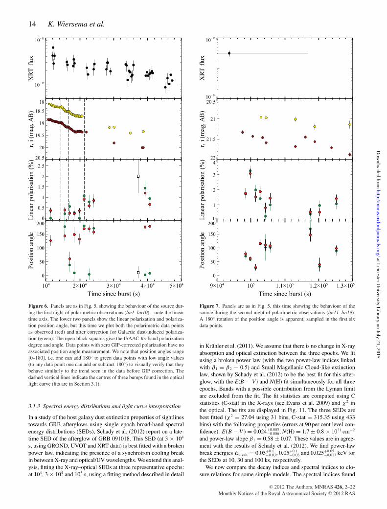
Figure 6. Panels are as in Fig. 5, showing the behaviour of the source dur-ing the first night of polarimetric observations (lin1–lin10) – note the lineartime axis. The lower two panels show the linear polarization and polariza-tion position angle, but this time we plot both the polarimetric data pointsas observed (red) and after correction for Galactic dust-induced polariza-tion (green). The open black squares give the ISAAC Ks-band polarizationdegree and angle. Data points with zero GIP-corrected polarization have noassociated position angle measurement. We note that position angles range[0–180], i.e. one can add 180◦ to green data points with low angle values(to any data point one can add or subtract 180◦) to visually verify that theybehave similarly to the trend seen in the data before GIP correction. Thedashed vertical lines indicate the centres of three bumps found in the opticallight curve (fits are in Section 3.1).

3.1.3 Spectral energy distributions and light curve interpretation

In a study of the host galaxy dust extinction properties of sightlinestowards GRB afterglows using single epoch broad-band spectralenergy distributions (SEDs), Schady et al. (2012) report on a late-time SED of the afterglow of GRB 091018. This SED (at 3 × 104

s, using GROND, UVOT and XRT data) is best fitted with a brokenpower law, indicating the presence of a synchrotron cooling breakin between X-ray and optical/UV wavelengths. We extend this anal-ysis, fitting the X-ray–optical SEDs at three representative epochs:at 104, 3 × 104 and 105 s, using a fitting method described in detail

Figure 7. Panels are as in Fig. 5, this time showing the behaviour of thesource during the second night of polarimetric observations (lin11–lin19).A 180◦ rotation of the position angle is apparent, sampled in the first sixdata points.

in Kruhler et al. (2011). We assume that there is no change in X-rayabsorption and optical extinction between the three epochs. We fitusing a broken power law (with the two power-law indices linkedwith β1 = β2 − 0.5) and Small Magellanic Cloud-like extinctionlaw, shown by Schady et al. (2012) to be the best fit for this after-glow, with the E(B − V) and N(H) fit simultaneously for all threeepochs. Bands with a possible contribution from the Lyman limitare excluded from the fit. The fit statistics are computed using Cstatistics (C-stat) in the X-rays (see Evans et al. 2009) and χ2 inthe optical. The fits are displayed in Fig. 11. The three SEDs arebest fitted (χ2 = 27.04 using 31 bins, C-stat = 315.35 using 433bins) with the following properties (errors at 90 per cent level con-fidence): E(B − V ) = 0.024+0.005

−0.006, N(H) = 1.7 ± 0.8 × 1021 cm−2

and power-law slope β1 = 0.58 ± 0.07. These values are in agree-ment with the results of Schady et al. (2012). We find power-lawbreak energies Ebreak = 0.05+0.1

−0.03, 0.05+0.1−0.03 and 0.025+0.05

−0.017 keV forthe SEDs at 10, 30 and 100 ks, respectively.

We now compare the decay indices and spectral indices to clo-sure relations for some simple models. The spectral indices found


at Leicester U



Dow

nloaded from



Figure 8. Upper panel: P/Pmax for a range of RV values, at the redshift ofGRB 091018 and using host galaxy extinction AV = 1 magnitude. Lowerpanel: resulting ratio of R-band and K-band linear polarization (in the casewhen all detected polarization is due to dust scattering in the host galaxy).

Figure 9. Emission lines of the [O II] doublet in the spectrum. The 2D spec-trum is shown in the top panel. Weak residuals from imperfect subtractionof sky emission lines can be seen as vertical stripes, also showing up asnarrow residuals in the 1D spectrum.

from the SED fits imply a power-law index for the electron energydistribution p = 2.16 ± 0.14. If the blast wave propagates in a ho-mogeneous density medium, the predicted afterglow decay indexfor the regime ν < νc is 3(p − 1)/4 = 0.87 ± 0.11, and for ν > νc itis 1.12 ± 0.11. A wind-like medium (where density decreases withr2) for ν < νc would imply α = (3p − 2)/4 = 1.37 ± 0.11, and

Figure 10. The optical light curve, in arbitrary flux units as describedin Section 3.1, is shown in blue (top), with the best fitting light curvesuperposed: a broken power law and three Gaussian components describingthe behaviour of flares. The red data points show the X-ray light curve, inunits of count rate, fitted with a double broken power law, see Section 3.1for the fit parameters.

Figure 11. X-ray–optical spectral energy distributions at three epochs (ob-server frame). Fits are done with a broken power law with a fixed differencebetween the two power-law spectral indices, and with the same X-ray ab-sorption and optical extinction for all three epochs.

for ν > νc it has the same index as for the homogeneous medium.The values for a homogeneous medium agree well with the valuesdetermined from the light curve fits (using the two-break model onthe XRT data) for the pre-break slopes, and are consistent with thepresence of a cooling break between X-ray and optical frequencies.In addition, in a wind-like medium the cooling break frequencyshould increase with time, which is not observed.

The break times in optical and X-rays are broadly in agreement,and the SEDs (Fig. 11; the first SED is before the break, the lastafter) show no evidence that the break is wavelength dependent(chromatic). As such, identifying this break with a jet break is com-pelling, particularly as this break is the second light curve break seenin the X-ray afterglow, with the first likely marking the end of en-ergy injection. However, we note that the post-break decay indices(1.33 ± 0.02 and 1.54 ± 0.15 for optical and X-rays, respectively)are too shallow compared to predictions from the standard fireball


at Leicester U



Dow

nloaded from



model, both in the case of non-sideways spreading jets (which pre-dicts post-break decay indices of 1.52 ± 0.11 for optical and 2.12 ±0.11 for X-rays) and sideways spreading jets (which should givepost-break decay indices of p).

An alternative interpretation could be that the break is not a jetbreak, but rather a break marking the start of the ‘normal’ afterglowphase, i.e. the decay indices after this break are pre-jet break indices,and the phase before this break is dominated by energy injection. Inthis case the post-break optical index of 1.33 ± 0.02 is consistentwith the closure relations in the case of a wind medium, which pre-dicts 1.37 ± 0.11. However, in that interpretation the optical decayindex should be steeper than the X-ray one, and the predicted X-raydecay index of 1.12 ± 0.11 is not consistent with the measurement.

We note that the homogeneous analyses of large samples of SwiftXRT afterglows have shown that a large fraction of afterglows withcandidate jet breaks (i.e. a light curve break significantly after aplateau phase) produce post-break decay indices that are too shallowcompared to simple model predictions (Willingale et al. 2007; Evanset al. 2009, their fig. 10; and Racusin et al. 2009, their fig. 2). Boththese papers further point out several additions to the models thatcan possibly explain some of this discrepancy, for example thepresence of low-level continuous energy injection past the plateauphase, or peculiar jet structure and sightline configurations. In thefollowing we will consider the observed break a candidate jet break,and will discuss alternative options as well.

If the break is a jet break, we can correct the isotropic energyEiso for beaming. Using Eiso = 3.7 × 1051 erg (Golenetskii et al.2009) and making the same assumptions as in Kocevski & Butler(2008), we find a jet opening angle θ jet ∼ 0.059 rad, or 3.◦4, leadingto log (Eγ ) ∼ 48.9. This is a fairly low value for Eγ , but not un-precedented: similar values are found for several other Swift bursts(Kocevski & Butler 2008) and pre-Swift bursts (Frail et al. 2001).

3.2 Circular polarization

The presence of a (weak) ordered magnetic field in addition to achaotic, incoherent magnetic field generated by the post-shock tur-bulence has been proposed (e.g. Granot & Konigl 2003) to explainthe non-detection of the swing in the linear polarization positionangle at the time of the jet break, expected in some models (e.g.Lazzati et al. 2003). In this picture, the observed polarization may bedominated by the weak large-scale ordered field, while emissivityis dominated by the random tangled field made by the post-shockturbulence. Polarization variability occurs as a result of changes inthe ratio of the ordered to random mean-squared field amplitudes(Granot & Konigl 2003). This results in much weaker changes in thepolarization and polarization position angle light curve around thejet break time. A direct test of this proposition can come from deepcircular polarization. Some searches have been performed at radiowavelengths during radio flares (Granot & Taylor 2005), but withfairly poor sensitivity (the best upper limit on circular polarizationis 9 per cent for GRB 991216).

Our data set contains four measurements of circular polarizationin optical, R-band, wavelengths, see Table 1, each with uncertaintiesof 0.15 per cent. Under the assumption that over the interval thatthe data were obtained (∼0.7 h, see Table 1) there is no changein circular polarization, we can combine these together. We find acombined value of the circular polarization Stokes parameter of v =V/I = −0.000 20 ± 0.000 75, which leads to a formal 2σ upper limitof Pcirc < 0.15 per cent: the deepest limit on circular polarization ofa GRB afterglow to date. Figs 4 and 6 show that during the circularpolarimetry epoch, the optical light curve shows a low-amplitude

bump. As such, the limit on the circular polarization can be seen asa limit on the circular polarization of the light of the bump plus thatof the underlying afterglow.

3.3 Interstellar polarization within the host galaxy

The variability of the detected linear polarization indicates that themajority of detected polarization can be associated with the after-glow. However, scattering of afterglow light on to dust grains withinthe host galaxy (host galaxy interstellar polarization – HGIP, follow-ing the terminology of Gorosabel et al. 2010) can induce noticeablelinear polarization, depending on the dust scattering geometry andgrain size distribution. This can affect attempts to interpret polariza-tion behaviour around jet breaks (e.g. Lazzati et al. 2003) or modelsusing the absolute level of polarization (e.g. Gruzinov & Waxman1999; Gruzinov 1999). For example, the zero polarization seen ine.g. lin1 could in principle be an unfortunate effect of HGIP on anintrinsically non-zero polarized afterglow.

We can utilize the reasonable assumption that over the opticalrange, the intrinsic afterglow linear polarization will be wavelengthindependent as it is synchotron emission, whereas HGIP will bestrongly wavelength dependent. In the Galactic ISM, the polariza-tion broadly follows an (empirical) relation known as the Serkowskilaw (Serkowski 1973):

Plin = Plin,max exp

(K ln2

(λmax

λ

)).

In this relation, Plin,max is the maximum induced linear polarizationat wavelength λmax. The wavelength λmax traces the size (distribu-tion) of the dust grains responsible for the observed polarization, andas such is closely linked to RV = AV /E(B − V). Klose et al. (2004)considered the effect of redshift in the Serkowski law, which resultsin a substitution λmax → (1 + z)λhost

max in the equation above, andthe relation λhost

max = RV /5.5. Klose et al. (2004) derive the observedlinear polarization Plin/Plin,max in standard photometric broad-bandfilters of an intrinsically unpolarized afterglow due to the presenceof dust in the host, as a function of redshift z and RV . Using theresults in Klose et al. (2004), we generate predictions for observedPlin/Plin,max in several broad-band filters as a function of RV , usingz = 0.971, shown in Fig. 8. From these, a predicted ratio Plin,R/Plin,K

is produced as a function of RV , plotted in the lower panel of Fig. 8.Multi-wavelength linear polarimetry has been possible for only asmall number of bursts: 020813 (Barth et al. 2003; Lazzati et al.2004), 021004 (Lazzati et al. 2003) and 030329 (Greiner et al. 2003;Klose et al. 2004). In these cases, no significant evidence for HGIPhas been observed.

Our Ks-band polarimetry is approximately simultaneous to theR-band polarimetry epoch lin9 (to be exact, lin9 is simultaneouswith linK3). The (GIP-corrected) Stokes parameters for lin9 andlinK are very similar, though we caution that the data were takenduring what appears to be a bump in the polarization light curve(Fig. 6). The resulting position angles are identical within errors,and we find Plin,R/Plin,K = 0.72 ± 0.45. This, combined with thestrong detected variation of both polarization degree and angle,demonstrates that (within errors) there is no indication of substantialHGIP contribution to the observed polarization. Martin & Angel(1976) demonstrate that the ISM induces a small degree of circularpolarization even in unpolarized sources. However, the levels ofinduced circular polarization are an order of magnitude or morebelow the limit we set in Section 3.2, considering the measuredGalactic GIP and the low extinction in the host galaxy (Section 3.1).


at Leicester U



Dow

nloaded from



In the following we therefore proceed with the assumption thatthe GIP-corrected polarization is all intrinsic to the source. In afuture paper (Paper 2) we will further quantify the implication ofthis measurement (and those of other GRB afterglows) on the dustand gas properties in GRB sightlines. A possibility that we willalso address in Paper 2 is the effect of dust destruction by the GRBand afterglow high-energy radiation, which may make the effect ofHGIP time dependent.

3.4 Linear polarization light curve

Our R-band linear polarimetric monitoring took place over threeobserving nights, as described in Section 2.1.1. The behaviour overthe first two nights is illustrated in Figs 6 and 7, shown in linear timecoordinate. On the third night only one deep, final, measurementwas taken.

In the first night (see Fig. 6), the source starts off with very low(consistent with zero, within the errors dominated by the uncertaintyin the GIP Stokes parameters) polarization, the lowest observed fora GRB afterglow to date. Following that, a broad, low-amplitudebump may be present in the polarimetric curve. GRBs 030329 and021004 showed a correlation between linear polarization behaviourand light curve bumps (e.g. Greiner et al. 2003). In Fig. 6 weindicate the times of the three bumps we find in our data. Somevariability may be present related to these bumps, but the statisticalsignificance is very low. After the first eight data points obtained atthe start of the night, observations were resumed at the end of thenight, showing a decline from a higher polarization level (Table 2),confirmed by the ISAAC polarimetry taken quasi-simultaneous tolin9. Over the first night, some low-level variation in position anglemay be present, but the uncertainties are large because of the lowlinear polarization: overall, the first night data are consistent with aconstant polarization angle.

The second night data (see Fig. 7) display short time-scale vari-ability: a polarization bump, peaking at �3 per cent polarization,accompanied by a clear rotation of the position angle. Followingthis, the end of the night shows a slow rise in polarization, accom-panied by further position angle variation. By the third night, theafterglow had become too faint for detailed sampling, and one deepdata point, lin20, was obtained (Table 2). This last data point clearlyshows low-level contribution from the host galaxy in the receivedlight. We will attempt to interpret the polarimetric data in Section 4.

3.5 Environment of the burst

In a forthcoming paper on this data set (Paper 2) we will analysethe GRB environment in detail. In this section we will derive someproperties most relevant to the afterglow physics, and to show thatthis burst displays no indications of being unusual.

In the late-time images taken with Gemini (see Table 3) the hostgalaxy can clearly be seen as an extended structure, see Fig. 12,visibly extended in the east–west direction. An isophote fit usingelliptical isophotes (using the ellipse package within IRAF) gavea best fit for an ellipse orientation of 89 ± 4◦. We determined theposition of the GRB within its host by performing image subtractionof the three Gemini epochs using a modified version of the ISIS2 code(Alard & Lupton 1998). We detected a clear afterglow residual ina subtraction of the first and third epoch, and between the first andsecond epochs. No residual was detected in a subtraction betweenthe second and third epochs. We found the GRB location to be offsetby approximately 5.8 kiloparsec from the centre of the galaxy (asfound from the elliptical isophote fits), see Fig. 12. This offset, as

Figure 12. The host galaxy of GRB 091018, from the second epoch Gem-ini GMOS r-band data. The dashed tickmarks mark the position of theGRB as determined from PSF-matched image subtraction of Gemini epochs1 and 2.

well as the observed host magnitude, r = 23.4 (AB; see Table 3), iswell within the observed distribution for long GRBs at this redshift(e.g. Bloom, Kulkarni & Djorgovski 2002; Savaglio, Glazebrook &LeBorgne 2009).

The X-shooter afterglow spectra show very strong absorp-tion lines (Fig. 13) composed of at least three discrete velocitycomponents, spanning ∼300 km s−1. No lines from intervening sys-tems are detected. At the GRB redshift we detect both common res-onance lines and a small number of transitions arising from excitedfine-structure and metastable levels (from Fe II and possibly Ni II),though the lines from these excited transitions are very weak inour spectrum. Time-resolved spectroscopy of GRB afterglows hasshown that these excited transitions are excited through indirect UVpumping (fluorescence) by the afterglow photons (e.g. Vreeswijket al. 2007). This unambiguously identifies the redshift z = 0.971to be that of the GRB.

The X-shooter spectra were taken with the slit position anglealigned with the parallactic angle, set at −90.◦8 at the start of ob-servations, and therefore oriented broadly along the host galaxy.In addition to absorption lines, we therefore also detect nebularemission lines in the spectrum (e.g. H α, [O II], [O III]), though theirsignal to noise is low as the afterglow strongly dominates the light(see Table 3). The detection of the resolved [O II] λλ 3726, 3729doublet is shown in Fig. 9. Its flux of ∼6 × 10−17 erg s−1 cm−2 canbe used to derive an estimate of the star formation rate (SFR): usingthe equation from Kennicutt (1998) we find an SFR ([O II]) ∼4 Mper year. If we instead use the empirical conversion from [O II] lineluminosity to SFT derived by Savaglio et al. (2009) for GRB hostgalaxies, we find SFR ([O II]) ∼1.6 M per year (note that no ex-tinction correction was applied to the [O II] line luminosity). ThisSFR ([O II]) is fairly typical for long GRB hosts (Savaglio et al.2009). In conclusion, the afterglow spectrum, host magnitude andmorphology, and star formation rate are all in line with expectationsfor a normal long GRB host galaxy.

In Paper 2 we will further analyse the spectrum and exploit therare opportunity where we can probe (interstellar) gas and dust inthe host galaxy using five methods simultaneously: through after-glow absorption lines (including excited fine-structure lines), neb-ular emission lines, afterglow SEDs, wavelength-dependent linearpolarimetry and host imaging.


at Leicester U



Dow

nloaded from



Figure 13. The UVB arm spectrum from X-shooter, smoothed with a 3 pixel boxcar for presentation purposes. Some commonly observed (resonance)absorption lines are indicated with red, solid, vertical lines and are labelled. The dash–dotted, blue, vertical lines mark the positions of excited fine-structuretransitions of Fe II, which are occasionally observed as highly variable lines in GRB afterglow spectra. The dotted, green, vertical lines mark the positions ofexcited fine-structure transitions of Ni II.

4 DISCUSSION

4.1 GRB 091018 compared to GRBs 030329, 021004, 020813,020405 and 090102

It is instructive to compare the properties of the polarization of theafterglow of GRB 091018 with those of the best studied previouscases: the pre-Swift bursts 030329 (z = 0.1687), 021004 (z = 2.323),020813 (z = 1.254) and 020405 (z = 0.690). Each has multiplemeasurements over more than one night. We also compare to Swiftburst 090102 (z = 1.547), which has only one single measurement,which probes the poorly explored early-time afterglow.

Both 021004 and 030329 have well-studied bumps in their after-glow light curves (021004: Bersier et al. 2003b; Fox et al. 2003;Holland et al. 2003; Mirabal et al. 2003; Pandey et al. 2003. 030329:Burenin et al. 2003; Matheson et al. 2003; Sato et al. 2003; Uemuraet al. 2003; Bloom et al. 2004; Lipkin et al. 2004), frequently at-tributed to late-time energy injection (late-time activity of the cen-tral engine). Both sources are pre-Swift bursts and therefore haverelatively poorly sampled X-ray light curves compared to burstsin the Swift era, but well-sampled optical and radio afterglows.GRB 030329 has the best sampled polarimetric light curve of anyburst to date, with polarization measurements extending to a monthafter burst (Greiner et al. 2003). The data show some correlationbetween the degree of linear polarization Plin and changes in the de-cay index of the afterglow (bumps), though Plin and the light curvedo not change strictly simultaneously (Greiner et al. 2003). Simi-larly, it appears that not every bump is associated with a polarizationchange. Variability in both position angle and polarization degreeis detected for 021004 (e.g. Lazzati et al. 2003; Rol et al. 2003),but an association with flare behaviour is not easy to make, in partbecause the polarimetric coverage is less dense than for 030329. Incontrast to 021004 and 030329, the afterglow of 020813 is smooth,and therefore this afterglow may be better suited to study global jetproperties. Similarly to 021004 and 030329, variability in polariza-tion is detected in 020813. GRB 091018 is the first Swift burst to jointhe small group of afterglows with observed polarimetric variability.

Bumps are observed in the broad-band optical light curves of thissource, but their amplitude is considerably less than those seen inthe afterglows of GRBs 021004 and 030329. If the bump amplitudecorrelates with polarization amplitude, we may expect the bumpsto have a smaller effect on the observed overall polarization and bein a better position to probe the properties of the jet as a whole.

GRB 020405 is of interest mainly because of the short time-scale variability with high polarization amplitude (nearly 10 percent polarization) that this source appears to show (Bersier et al.2003a; Covino et al. 2003), though near simultaneous measurementsdescribed in Masetti et al. (2003) do not confirm this behaviour. Nojet break was seen in the afterglow light curve, and the polarizationcurve could not be reconciled with standard models.

Jetted fireball models predict a clear change in polarization prop-erties around the jet break time. The behaviour of Plin and the po-larization position angle depends sensitively on the angle betweenthe jet axis and the observer, the internal structure of the jet, themagnetic field properties within the jet and whether or not sidewaysspreading of the jet occurs at around the jet break time (e.g. Rossiet al. 2004 and references therein). Attempts to fit these modelsto afterglow polarization data have been a little disappointing: in030329 and 021004 the bumps in the light curve may have influ-enced the fits (see e.g. Lazzati et al. 2003), whereas the polarimetricsampling of 020813 was rather too low to favour a single jet model,though several models could be excluded (Lazzati et al. 2004). Theafterglow of 020405 unfortunately shows no jet break within theinterval of polarimetric monitoring. The very well sampled 030329has the relative disadvantage of a bright supernova contributing atlate times, in addition to the bumps at early times, and determininga unique jet break time proved complicated (with best model likelyrequiring two jet breaks, see e.g. Van der Horst et al. 2008 and refer-ences therein). Our data of 091018 may therefore be one of the firstcases where a jet break can be probed in some detail through po-larimetry, if the light curve break discussed in Section 3.1 is indeeda jet break.

Our polarimetric follow-up starts at rest-frame time 0.067 d(5782 s) after burst trigger, considerably earlier than the earliest data


at Leicester U



Dow

nloaded from



points of 030329, 021004 and 020813. It is clear that polarimetryvery early after burst requires automated/robotic procedures. Usingsuch an approach, a very early afterglow polarimetric detection ofGRB 090102 was obtained by Steele et al. (2009), who secure adetection of Plin = 10.2 ± 1.3 per cent at rest-frame time 75 s afterburst, using the robotic Liverpool Telescope. Such a high degree ofpolarization, measured when the reverse shock component was stillbright, is consistent with the presence of large-scale ordered mag-netic fields. Although our data on 091018 are taken considerablylater in time than those on 090102, the superb sensitivity of the VLTmay allow us to continue to probe the magnetic field structure at latetime through our high-precision linear and circular polarimetry.

4.2 GRB 091018 and models

4.2.1 Reverse shock

The start of our polarimetric monitoring was sufficiently late thata contribution of reverse shock emission to the received light islikely negligible. While this precludes study of some magnetizationproperties (e.g. Granot & Taylor 2005), this makes a comparisonof the data with models easier, as only a forward shock modelneeds to be considered. The low linear polarization at the startof our monitoring appears to confirm this: emission from reverseshocks is expected to be considerably polarized, as the shock travelsback into magnetized shocked material (e.g. Granot & Taylor 2005;Steele et al. 2009).

4.2.2 Jet break

We compare our data with the model series computed by Rossiet al. (2004), hereafter referred to as R04, who derive the expectedlinear polarization curves (including position angle) for a grid ofdifferent jet model parameters, assuming that there is no additionalcoherent component of the magnetic field present and that HGIP isnegligible. In particular, R04 consider the cases of homogeneousjets, structured jets and Gaussian jets, each with a grid of differentviewing angles (in the case of homogeneous jets this is the angle theline of sight makes with the jet axis), and for a range of wavelengthsand physical parameters. They further distinguish jet breaks withand without sideways spreading.

We can briefly summarize the main differences between the var-ious models as found by R04, and refer for details and explanationsto that paper (see also fig. 18 of R04):

(i) Homogeneous jets show two peaks in the polarization curves,with the second peak always reaching a higher polarization thanthe first. Structured and Gaussian jets show one peak only, withpeak time for a Gaussian jet significantly later than for a structuredjet, which has its peak around the time of the break. The peaks ofthe structured and Gaussian jets are much wider than the ones forhomogeneous jets (i.e. rise time and decay time-scales are long).

(ii) The position angle for a homogeneous jet changes by 90◦ inbetween the two peaks in the polarization curves: the two peakseach have constant position angle, but are 90◦ different. Structuredand Gaussian jets have constant position angles throughout.

(iii) Structured jets show non-negligible polarization at earlytimes, whereas homogeneous jets and Gaussian jets have zero po-larization at early times.

(iv) The shape of the bumps in the different jet structures isdifferent.

Figure 14. All GIP-corrected linear polarization data plotted as a functionof the time since burst divided by the time of the break in the optical lightcurve (i.e. tbreak = 3.23 × 104 s). Overplotted in blue is the model (fromRossi et al. 2004) for a homogeneous jet with a jet break at tbreak that doesnot experience sideways expansion, with viewing angle θobs = 0.2θ jet. Themodel has been shifted slightly (by dividing the model t/tjet by 1.15). Thelower panel shows the polarization position angle. The dotted line for t/tjet <

1.5 shows the average position angle (6◦). The dotted line for t/tjet > 1.5 isset at 96◦: the average value before this time plus 90◦, to show the predicted90◦ position angle swing. The inset shows the rapid polarization rotation att/tbreak ∼ 3.16 (vertical dotted line in the inset), with the horizontal dottedline at a position angle of 96◦.

(v) Sideways expanding jets show lower polarization values thannon-sideways expanding jets (all other parameters being equal),with wider bump(s) in the polarization curve.

We start by evaluating the data in time coordinates normalized bythe time of the break seen in the optical data (see Section 3.1). It isclear that some polarization behaviour is observed occurring closeto t/tbreak ∼ 1, as expected for jet breaks. In the case when this breakis a jet break, we can then directly compare the curves with thosein R04. Fig. 14 shows a plot in these units. Comparing to the points(i)–(v) listed above, there appears to be evidence that a model withconstant position angle throughout will not provide a good fit; early-time polarization is consistent with zero (or at least is lower thanpredictions for structured jets); a single bump model with a shape aspredicted by the models in R04 seems inconsistent with the data. InFig. 14 we therefore plot a model for a homogeneous, non-sidewaysexpanding jet with viewing angle θobs = 0.2θ jet (from fig. 8 in R04).We shift this curve slightly in time coordinate by dividing t/tjet by1.15 to get a better visual match. The first bump in the polarizationcurve appears to be well reproduced in both shape and amplitude,including the zero polarization at early times. This model predicts aconstant polarization position angle over the first bump. We indicatein Fig. 14 (dotted line) the average of the position angle at t/tbreak �1.4. As required by the R04 model, the position angle is constantover this bump.

The second bump predicted by the homogeneous jet model shouldhave a larger amplitude than the first, a position angle 90◦ offset fromthe first bump and a morphology opposite to the first (in coordinatesused in Fig. 14). Some of the data points indeed have a higherpolarization than seen in the first bump, but the morphology of thebump as predicted by the model is not observed. We examine thebehaviour of the position angle by adding 90◦ to the position anglefor t/tbreak � 1.4. In Fig. 14 this is the second horizontal dotted line.It is clearly seen that the value of the position angle is overall higherthan in the first bump, but is not constant as the model predicts,showing considerable variability on a short time-scale (possiblyvarying around the predicted position angle), including a rotationof the position angle visible in the interval t/tbreak ∼ 3.0–3.3. The


at Leicester U



Dow

nloaded from



polarization curve shows, compared to the homogeneous jet model,a deep short dip, in the interval t/tbreak ∼ 3–4. This dip shows avery steep decay in the first few data points, simultaneous with theobserved rotation in position angle. This behaviour is not predictedby any jet break model.

We could consider the possibility that there is an additional polar-ization curve component (hereafter simply referred to as the extracomponent) on top of a slower behaviour as predicted by jet breakmodels. A third smooth, fairly narrow, polarized bump peaking ataround t/tbreak ∼ 3–4 could be present, having a position angle sig-nificantly offset from the θ = 96◦ of the second bump from thehomogeneous jet model. The sum of this component and that of the(second bump of the homogeneous) jet model can give rise to mostof the observations: the steep dip, where the contributions of the twocomponents nearly cancel due to differing position angles, and therotation in position angle, where the components are at similar am-plitude but very different position angle. However, this is a ratherdegenerate problem, as the amplitude as a function of time (theshape) of the extra component and the position angle as a functionof time are all unknown. A component with a fixed position anglebut variable amplitude (i.e. a component much like the polarizationpeaks from a jet break) can approximate the data (with a position an-gle ∼70◦ offset from the constant 96◦, and peaking around t/tbreak ∼3.5), but a component with nearly constant amplitude but positionangle varying on very short time-scales can provide a reasonableapproximation too. Wu et al. (2005) evaluate the expected polar-ization curves of afterglows from two-component jets (as proposedfor e.g. 030329, Berger et al. 2003), which show, as expected, alarge variety of behaviour, depending mostly on viewing angle andcontrast between the narrow and wide jet components. However,the observed variability in the data of 091018 around t/tbreak ∼ 3–4is much more rapid than predicted by the models of Wu et al.(2005). At the current data quality, and including the uncertainty inand applicability of the underlying model (homogeneous jet modelfrom R04), we are not in a position to quantify the behaviour of thisputative component further. As the shape of the bump and time vari-ability of the position angle are unclear, it is difficult to speculateon the possible origin of such an additional component. The featureoccurs after the expected time of the peak of the second bump inthe R04 model and no such feature is visible at t < tbreak. As such,it may be related to a discrete bright region (patch) on the jet thatcomes into view just after the second bump peaks. In this scenariowe may expect a constant position angle of the component producedby the patch (if the field in the patch is coherent), with a bump shapereflecting the brightness profile of the bright patch. However, otherexplanations, such as microlensing, two-component jets or others,are difficult to rule out with the polarization data alone.

The time-span possibly most affected by the extra component,t/tbreak ∼ 3–4, corresponds to 9.7–12.9 × 104 s. In the optical lightcurves no significant slow variability at around that time is obvious.The XRT data show a possible broad, slow softening around thistime, but our SED fits do not point to strong spectral variation atthis time. The shallow post-break decay indices and/or the flaresobserved in the optical light curve (Section 3.1) may be related tothe observed polarization behaviour, i.e. be linked to the observedextra component, but further modelling will be required to testthis.

There is at least one other source that shows a variability in thepolarization curve on short time-scales (intranight) and unrelatedto a jet break, GRB 020405. However, in that source only a sin-gle data point showed the deviation from a constant polarizationdegree (Bersier et al. 2003a), and the position angle was not seen

to vary over the available polarization measurements. No featuresresembling jet break bumps were detected in that source, consistentwith the absence of a jet break in the light curves. The possibledetection of a variation at fairly short time-scales, with possibly aconstant position angle and likely unrelated to a jet break in GRB091018 (the extra component in the polarization curve) may be anindication that this type of behaviour is indeed real.

The conclusion from the above discussion is that none of the sim-ple models of polarization behaviour of GRBs directly reproducesthe observed behaviour. Of the available models, the homogeneousjet break model comes closest, but requires at least one additionalcomponent, the nature of which is currently unknown.

4.2.3 Ordered fields

The circular polarization upper limit derived in Section 3.2 can beused to probe large-scale ordered fields, which have been proposedby several authors to explain various phenomena, such as the highlinear polarization at very early times (Steele et al. 2009), or the lackof obvious polarization position angle shifts around the jet breaktime for e.g. GRBs 030329 and 021004 (Granot & Konigl 2003).Models of the expected circular polarization in optical wavelengthsfor an external shock (Matsumiya & Ioka 2003; Sagiv et al. 2004;Toma, Ioka & Nakamura 2008) generally find that afterglows shouldshow very low circular polarization in the absence of strong large-scale ordered fields. Our detection limit of Pcirc < 0.15 per cent isin full agreement with these predictions (see e.g. Toma et al. 2008)and excludes strong ordered field components. We note the timingof our circular polarimetry: our data were taken when the reverseshock emission is likely negligible, and when the linear polarizationwas still very weak. It is clear that it is not easy to significantlyimprove on the depth of this limit in optical wavelengths, but itwould be interesting to search for circular polarization in otherbursts, to establish whether this is a common feature, and to searchfor circular polarization at early times when reverse shock emissionis still present.

4.2.4 Energy injection

An alternative explanation of the observed break in the light curvesis that this break marks the end of (continuous) energy injection,though the post-break decay indices are not as expected from theclosure relations (Section 3.1). The occurrence of significant po-larimetric variability at around t/tbreak ∼ 1 indicates that if thisscenario is correct, the end of energy injection must be accompa-nied by a geometric change, as the polarization position angle staysconstant. In a study of GRB 021004, Bjornsson, Gudmundsson &Johannesson (2004) model the strong rebrightenings visible in theafterglow light curve with discrete, powerful, energy injections anddemonstrate that the light curves are fairly well reproduced thisway. They demonstrate that their model shows some correlationwith the polarimetric data, i.e. that polarization is related to bumps.For GRB 030329, Greiner et al. (2003) come to a similar conclusionfrom their data. We see at least three low-amplitude bumps in theoptical light curve, at times given in Section 3.1, but a correlationwith polarimetric behaviour is not clearly visible, largely because ofthe larger uncertainties in our polarization values compared to themuch brighter afterglow of 030329. Similarly, a possible relationbetween the extra component in the polarization curve and the flar-ing around the jet break time is unclear. Future (numerical) modelsof light curve bumps/flares (e.g. Vlasis et al. 2011) and high-quality


at Leicester U



Dow

nloaded from



data (e.g. Kruhler et al. 2009) may provide the possibilities of com-puting expected polarization signals from the simulations. Thesemay then be used to understand the connection between the physi-cal parameters behind these bumps and the behaviour in polarizedlight.

5 C O N C L U S I O N S

We presented a large polarimetry data set of the afterglow of GRB091018, and add to that an extensive multicolour photometric dataset and medium resolution spectroscopy. We find an abundance ofabsorption lines in the spectrum of the afterglow as well as a fewemission lines, from which we find a redshift z = 0.971. The X-ray light curve shows at least two breaks, as well as a complexof flaring activity. The densely sampled optical light curve showsseveral flares as well, and through a fit using a broken power lawand three Gaussian components (to describe the flares), we find anachromatic break at tbreak ∼ 3.2 × 104 s. Our polarization data coverthis break, allowing us to probe its nature using linear polarimetry.Our polarimetry results can be summarized as follows.

(i) In contrast to GRBs 030329 and 021004, there are no strongrebrightenings that confuse our view of the polarization behaviour.

(ii) Our deep circular polarimetry at t ∼ 0.15 d after burst showsno circular polarization, with 2σ limit Pcirc < 0.15 per cent.

(iii) The quasi-simultaneous R- and Ks-band polarimetry showsno strong indications of a considerable contribution of polarizationfrom the ISM in the host galaxy.

(iv) The linear polarimetry shows a constant position angle fort/tbreak < 1.4, and a considerably higher, but strongly variable, valuethereafter.

(v) At least two peaks are present in the polarization curve. Thefirst of these, as well as the constant position angle, is well repro-duced by a model of a jet break using a homogeneous, non-sidewaysspreading jet with small viewing angle (from R04).

(vi) If the observed break is a jet break, and if the model of ahomogeneous, non-sideways spreading jet is correct, an additionalcomponent is required to reproduce the observed polarization curveand position angles. This may be a short-duration bump with con-stant position angle, offset from the position angle of the underlyingjet break component.

From the above it is clear that the models for polarization be-haviour around the time of jet break (as in R04) cannot, in theircurrent form and on their own, explain the full behaviour of thepolarization curve of 091018. Further modelling efforts, in particu-lar into the effects of rebrightenings/bumps and continuous energyinjection on the observed polarization, are vital to exploit the fullpotential of polarimetry as probe of afterglow physics.

These results are the first of their kind for Swift GRBs, and indeedGRB 091018 can be considered a ‘normal’ GRB, with none of itsprompt emission or afterglow properties particularly remarkable,in contrast to some of the polarimetrically studied pre-Swift burstslike 030329. This is in part because our selection criteria of sourcesto study with polarimetry were only that: the source had to be aSwift burst with a detected afterglow in both XRT and UVOT data.This avoids a bias towards the brightest or slowest decaying opticalafterglows, and indeed it is clear from Section 3.1 that GRB 091018is one of the faintest afterglows with multi-night polarimetry. Fur-ther, similar observations of (Swift) bursts with different micro- andmacro-physical parameters (in particular energetics, jet opening an-gle, density n and density gradient k) will be required to establish

whether or not GRB 091018 is representative of the sample of GRBafterglows as a whole.

Unfortunately, no long-wavelength (radio, (sub-)mm) observa-tions were available for GRB 091018. A deep polarimetric cam-paign on an afterglow, with radio and (sub-)mm light curve data inaddition to optical and X-ray light curves, would be particularly in-teresting, since with the resulting broad-band SEDs (with sensitivityredwards of the synchrotron peak frequency νm) we would be ableto fit for parameters that are particularly relevant for polarimetricinterpretations, e.g. εE and εB.

AC K N OW L E D G M E N T S

We warmly thank the ESO staff for obtaining the VLT data discussedhere. We thank Justyn Maund, Dave Russell, Daniele Malesani,Piergiorgio Casella, Elena Rossi, Christina Thone and AlexanderKann for their help and useful discussions. We thank the anonymousreferee for useful comments and suggestions. Based on observationsmade with ESO Telescopes at the Paranal Observatory under pro-grammes 084.D-0949 and 084.A-0260. KW acknowledges supportfrom STFC. TK acknowledges support by the European Commis-sion under the Marie Curie Intra-European Fellowship Programme.The Dark Cosmology Centre is funded by the Danish NationalResearch Foundation. RLCS is supported by a Royal Society Fel-lowship. The financial support of the British Council and PlatformBeta Techniek through the Partnership Programme in Science (PPSWS 005, PI: Wiersema) is gratefully acknowledged. Part of thefunding for GROND (both hardware as well as personnel) wasgenerously granted from the Leibniz-Prize to Prof. G. Hasinger(DFG grant HA 1850/28-1). SK and AR acknowledge support byDFG grant Kl 766/16-1, and AR in addition from the BLANCE-FLOR Boncompagni-Ludovisi, nee Bildt foundation. This workmade use of data supplied by the UK Swift Science Data Centreat the University of Leicester. IRAF is distributed by the NationalOptical Astronomy Observatory, which is operated by the Asso-ciation of Universities for Research in Astronomy (AURA) undercooperative agreement with the National Science Foundation.

R E F E R E N C E S

Alard C., Lupton R. H., 1998, ApJ, 503, 325Barth A. et al., 2003, ApJ, 584, 57Berger E. et al., 2003, Nat, 426, 54Bersier D. et al., 2003a, ApJ, 583, L63Bersier D. et al., 2003b, ApJ, 584, L43Bjornsson G., Gudmundsson E. H., Johannesson G., 2004, ApJ, 615, L77Bloom J. S., Kulkarni S. R., Djorgovski S. G., 2002, AJ, 123, 1111Bloom J. S., van Dokkum P. G., Bailyn C. D., Buxton M. M., Kulkarni S.

R., Schmidt B. P., 2004, AJ, 127, 252Burenin R. A. et al., 2003, Astron. Lett., 29, 573Cardelli J. A., Clayton G. C., Mathis J. S., 1989, ApJ, 345, 245Chandrasekhar S., 1960, Radiative Transfer. Dover, New YorkChen H.-W. et al., 2009, GCN Circ. 10038Costa E. et al., 1997, Nat, 387, 783Covino S. et al., 2003, A&A, 400, L9Curran P. A. et al., 2007a, MNRAS, 381, 65Curran P. A. et al., 2007b, A&A, 467, 1049Cushing M. C., Vacca M. D., Rayner J. T., 2004, PASP, 116, 362Evans P. A. et al., 2009, MNRAS, 397, 1177Filgas R., Kruhler T., Yoldas A., Klose S., Greiner J., 2009, GCN Circ.

10039Fossati L., Bagnulo S., Mason E., Landi Degl’Innocenti E., 2007, in

Sterken C., ed., ASP Conf. Ser., Vol. 364, The Future of Photometric,


at Leicester U



Dow

nloaded from



Spectrophotometric and Polarimetric Standardization. Astron. Soc. Pac.,San Francisco, p. 503

Fox D. W. et al., 2003, Nat, 422, 284Frail D. A. et al., 2001, ApJ, 562, L55Gehrels N. et al., 2004, ApJ, 611, 1005Gehrels N., Ramirez-Ruiz E., Fox D. B., 2009, ARA&A, 47, 567Ghisellini G., Lazzati D., 1999, MNRAS, 309, L7Goldoni P., Royer F., Francois P., Horrobin M., Blanc G., Vernet J.,

Modigliani A., Larsen J., 2006, SPIE, 6269, 80Golenetskii S. et al., 2009, GCN Circ. 10045Gorosabel J. et al., 2010, A&A, 522, 14Granot J., Konigl A., 2003, ApJ, 594, L83Granot J., Taylor G. B., 2005, ApJ, 625, 263Greiner J. et al., 2003, Nat, 426, 157Greiner J. et al., 2008, PASP, 120, 405Greiner J. et al., 2011, A&A, 526, 30Gruzinov A., 1999, ApJ, 525, L29Gruzinov A., Waxman E., 1999, ApJ, 511, 852Holland S. T. et al., 2003, AJ, 125, 2291Joos F., Buenzli E., Schmid H. M., Thalmann C., 2008, SPIE, 7016, 70161I-1Kennicutt R. C., 1998, ARA&A, 36, 189Klose S., Palazzi E., Masetti N., Stecklum B., Greiner J., Hartmann D. H.,

Schmid H. M., 2004, A&A, 420, 899Kocevski D., Butler N., 2008, ApJ, 680, 531Kouveliotou C., Meegan C. A., Fishman G. J., Bhat N. P., Briggs M. S.,

Koshut T. M., Paciesas W. S., Pendleton G. N., 1993, ApJ, 413, L101Kruhler T. et al., 2009, ApJ, 697, 758Kruhler T. et al., 2011, A&A, 534, 108LaCluyze A. et al., 2009, GCN Circ. 10061Lazzati D., 2006, New J. Phys., 8, 131Lazzati D. et al., 2003, A&A, 410, 823Lazzati D. et al., 2004, A&A, 422, 121Lipkin Y. M. et al., 2004, ApJ, 606, 381Markwardt C. B. et al., 2009, GCN Circ. 10040Martin P. G., Angel J. R. P., 1976, ApJ, 207, 126Martin P. G., Whittet D. C. B., 1990, ApJ, 357, 113Masetti N. et al., 2003, A&A, 404, 465Matheson T. et al., 2003, ApJ, 582, L5Matsumiya M., Ioka K., 2003, ApJ, 595, L25Meszaros P., Rees M. J., 1992, MNRAS, 257, 29Meszaros P., Rees M. J., 1997, ApJ, 476, 232Mirabal N. et al., 2003, ApJ, 595, 935Mundell C. G. et al., 2007, Sci, 315, 1822

Nousek J. et al., 2006, ApJ, 642, 389Pandey S. B. et al., 2003, Bull. Astron. Soc. India, 31, 19Patat F., Romaniello M., 2006, PASP, 118, 146Piran T., Fan Y.-Z., 2007, Phil. Trans. R. Soc. A., 365, 1151Racusin J. L. et al., 2009, ApJ, 698, 43Rhoads J. E., 1997, ApJ, 487, 1Rhoads J. E., 1999, ApJ, 525, 737Rol E. et al., 2003, A&A, 405, L23Roming P. W. A. et al., 2005, Space Sci. Rev., 120, 95Rossi E. M., Lazzati D., Salmonson J. D., Ghisellini G., 2004, MNRAS,

354, 86 (R04)Sagiv A., Waxman E., Loeb A., 2004, ApJ, 615, 366Sari R., 1999, ApJ, 524, 43Sari R., Piran T., Halpern J. P., 1999, ApJ, 519, L17Sato R. et al., 2003, ApJ, 599, L9Savaglio S., Glazebrook K., LeBorgne D., 2009, ApJ, 691, 182Schady P. et al., 2012, A&A, 537, 15Serkowski K., 1973, in Greenberg J. M., van de Hulst H. C., eds, IAU Symp.,

52. Interstellar Dust and Related Topics. Reidel, Dordrecht, p. 145Serkowski K., Matheson D. L., Ford V. L., 1975, ApJ, 196, 261Simmons J. F. L., Stewart B. G., 1985, A&A, 142, 100Sparks W. B., Axon D. J., 1999, PASP, 111, 1298Stamatikos M. et al., 2009, GCN Circ. 10034Steele I. A., Mundell C. G., Smith R. J., Kobayashi S., Guidorzi C., 2009,

Nat, 462, 767Toma K., Ioka K., Nakamura T., 2008, ApJ, 673, L123Uemura M. et al., 2003, Nat, 423, 843Ukwatta T. N. et al., 2012, MNRAS, 419, 614Van der Horst A. J. et al., 2008, A&A, 480, 35van Paradijs J. et al., 1997, Nat, 386, 686Vlasis A., van Eerten H. J., Meliani Z., Keppens R., 2011, MNRAS, 415,

279Vreeswijk P. M. et al., 2007, A&A, 468, 83Wardle J. F. C., Kronberg P. P., 1974, ApJ, 194, 249Wiersema K., 2011, MNRAS, 414, 2793Wijers R. A. M. J., Galama T. J., 1999, ApJ, 523, 177Willingale R. et al., 2007, ApJ, 662, 1093Witzel G. et al., 2011, A&A, 525, 130Wu X. F., Dai Z. G., Huang Y. F., Lu T., 2005, MNRAS, 357, 1197

This paper has been typeset from a TEX/LATEX file prepared by the author.


at Leicester U



Dow

nloaded from


Detailed optical and nearinfrared polarimetry ... · and broad-band photometry of the afterglow of...

Documents

Transcript of Detailed optical and nearinfrared polarimetry ... · and broad-band photometry of the afterglow of...