Designing Sundials by Matlab and Maple - TUTruohonen/SundialRep.pdf · Designing Sundials by Matlab...

1

Designing Sundials by Matlab and Maple

KEIJO RUOHONEN

Institute of MathematicsTampere University of Technology

33101 Tampere, [email protected]

(original version 1995)

Contents

2 1. Introduction4 2. Some Basic Constructs6 3. A Solar Time Sundial16 4. The Equation of Time24 5. An Equatorial Mean Solar Time Sundial52 6. Timeshifts64 7. A Nonequatorial Mean Solar Time Sundial

67 References

2

1. Introduction

The ancient art of sundial designing and making has produced an astonishingvariety of designs, many of them ingenious and works of art. The history and afair sample of various designs can be found in [Ro] or [Pe,Sch,SP]. The principlesof working are in many cases forgotten and understood only by a very tedious re-verse-engineering, often made much more difficult by well-meant but incompe-tent repair work. This is the case e.g. for the famous Schissler bowl sundial,made in 1578, see [Sa].

Nowadays investigating sundials cannot be considered an important undertak-ing. Nevertheless, the art is not dead. Some of the more advanced mean solartime showing sundials are of relatively recent origin, see [Ro,Lo]. The “missing”latitude-independent sundial was first described in [Fr]. (Any three of the fourvariables altitude, declination, azimuth—related to Sun’s position in the sky—and latitude determine the fourth, so in principle only three of them are neededto set up a sundial.)

The goal of the present paper is to show that use of mathematics programs canbe a central tool in invigorating the art of sundial designing. The central princi-ple here is to use throughout the usual equal-hour 24 h clock face. This has theconsequence that the shadow must be created by a rather complex surface. Gen-erating pictures of these surfaces requires much numerical computation. Theprograms Matlab® and Maple® are used here (actually much of Maple appearsas a toolbox of Matlab). As theoretical tool, vector calculus is used. It is stronglyfelt that the more usual method of spherical trigonometry has had its time.

The paper is organized as follows. In Section 2 general principles for designingand computing shadow caster surfaces are given. In Section 3 a solar time sun-dial design is obtained and investigated by Maple. The design is further refinedin Section 6. Then in Section 4 the equation of time, giving the difference be-tween mean solar time and solar time, is constructed and consequently used inSection 5 for designs of various equatorial mean solar time sundials. The surpris-ing difficulties appearing in such designs are thoroughly discussed. The tool hereis Matlab. In Section 7 an attempt to extend the ideas of Section 5 to nonequa-torial sundials is taken, without much success.

The codes listed here are stripped of comments (which appear in the text). Notmuch effort is taken to optimize the codes, as they are reasonably fast and prob-ably are not run repeatedly. It would be possible to obtain much faster codes byintegrating numerical quadrature and plot file generation, say.

® Matlab is trademark of The Mathworks Inc.. Maple is trademark Waterloo MapleSoftware.

3

2. Some Basic Constructs

The sundial, Earth and Sun are positioned originally in a xyz-coordinate systemwhere

(i)(ii)

(iii)

(iv)

(v)

the origin is in the centre of Earth,the xy-plane is the equatorial plane,the z-axis is oriented along Earth’s axis, the north pole being on the pos-itive z-axis,at noon Sun is in the yz-plane,the sundial is a circle in the xy-plane with radius 1 and centre in the ori-gin,the time scale is the usual linear 24 hour scale and is read clockwisearound the perimeter of the circle with the 12 o’clock mark being on thenegative y-axis.

Thus the original situation is as is Figure 1. Inthe sequel the time is given in radians, i.e., theangle w corresponds to

12 1 24

wπ

+

(mod )

hours, and to the point (–sin w,–cos w,0) on thedial circle.

Sun

x

y

w1

Figure 1

It will be allowed that the sundial may be tilted, i.e., rotated by an angle δaround x-axis. After this operation the point corresponding to time w will be

p( ) cos sinsin cos

sincos

sincos cos

sin cos

www

ww

w=

−

−−

=−

−

1 0 000 0

δ δδ δ

δδ

.

Thus at noon the situation is as depicted in Fig-ure 2 where σ is Sun’s declination.

There are many choices for the time. If Earth’srotation angle is given by v, then the simplestchoice is the solar time given by w = v . Otherchoices are the mean solar time, to be treatedlater, and, say, a local time, daylight savings

Sun

y

z

σδ

sundial

Figure 2

time or sidereal time. In these cases w depends on v and possibly some other pa-

4

rameter, e.g. Sun’s declination σ or (through σ) Earth’s polar angle φ in the eclip-

tic. w is then a function of v and σ or of v and φ.

As concerns measurement and definitions of the various concepts of time in gen-eral, [AA], [Se] and [HS] are recommended.

The time is indicated by a shadow cast on the perimeter of the sundial by a sur-face. This surface has the property that a ray from Sun to the point p(w) touchesthe surface. Now, since this ray is given by

p(w) + λd(v,σ)

where

d( )cos sinsin cos cos

sin

sin coscos cos

sin

vv vv v

vv,σ σ

σ

σσ

σ= −

=

00

0 0 1

0,

the surface has the parametric representation

r(v,σ) = p(w(v,σ)) + λ(v,σ)d(v,σ)

for a properly chosen function λ(v,σ) (actually the distance from p(w) to the point

where the ray touches the surface). The function λ(v,σ) can be found by demand-

ing that the normal of the surface is perpendicular to d(v,σ), i.e., setting

0 = rv × rσ • d = (p′wv + λvd + λdv) × (p′wσ + λσd + λdσ) • d

= λwvp′ × dσ • d – λwσp′ × dv • d + λ2dv × dσ • d.

Thus

λ σ σ

σ= ′ × − •

× •p d d d

d d d( )w wv v

v.

Of course, this surface is also the envelope of the one-parameter family of sur-faces given by q(v,σ,λ) = p(w(v,σ)) + λd(v,σ), and λ(v,σ) can be found by setting

det(q′(v,σ,λ)) = 0 and solving for λ.

5

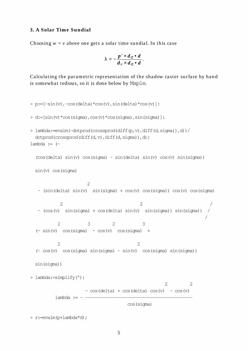
3. A Solar Time Sundial

Choosing w = v above one gets a solar time sundial. In this case

λ σ

σ= − ′ × •

× •p d dd d dv

.

Calculating the parametric representation of the shadow caster surface by handis somewhat tedious, so it is done below by Maple.

> p:=[-sin(v),-cos(delta)*cos(v),sin(delta)*cos(v)]:

> d:=[sin(v)*cos(sigma),cos(v)*cos(sigma),sin(sigma)]:

> lambda:=evalm(-dotprod(crossprod(diff(p,v),diff(d,sigma)),d))/

dotprod(crossprod(diff(d,v),diff(d,sigma)),d);

lambda := (-

(cos(delta) sin(v) cos(sigma) - sin(delta) sin(v) cos(v) sin(sigma))

sin(v) cos(sigma)

2

- (sin(delta) sin(v) sin(sigma) + cos(v) cos(sigma)) cos(v) cos(sigma)

2 2 /

- (cos(v) sin(sigma) + cos(delta) sin(v) sin(sigma)) sin(sigma)) /

/

2 3 2 3

(- sin(v) cos(sigma) - cos(v) cos(sigma) +

2 2

(- cos(v) cos(sigma) sin(sigma) - sin(v) cos(sigma) sin(sigma))

sin(sigma))

> lambda:=simplify(");

2 2

- cos(delta) + cos(delta) cos(v) - cos(v)

lambda := - -------------------------------------------

cos(sigma)

> r:=evalm(p+lambda*d);

6

r := [ - sin(v) - %1 sin(v), - cos(delta) cos(v) - %1 cos(v),

%1 sin(sigma)

sin(delta) cos(v) - ------------- ]

cos(sigma)

2 2%1 := - cos(delta) + cos(delta) cos(v) - cos(v)

> map(factor,r); [ - sin(v) (cos(v) - 1) (cos(v) + 1) (cos(delta) - 1),

3 - cos(v) (cos(delta) - 1),

- (- sin(delta) cos(v) cos(sigma) - sin(sigma) cos(delta)

2 2 + sin(sigma) cos(delta) cos(v) - cos(v) sin(sigma))/cos(sigma) ]

Thus this surface has the parametric representation

x vy vz z

= − −= −=

( cos )sin( cos )cos,

11

3

3δ

δ

i.e., it is an astroidal cylinder with maximum radius 1 – cos δ. It is noticed that

λ δσ

= +cos sin coscos

2 2v v

is nonnegative if and only if cos δ –cot 2v. Thus this construct is valid for

–π/2 ≤ δ ≤ π/2. Bounds for the values of z are also of interest, at least from the

point of view of practical sundial making. Now

z = sin δ cos v + (cos δ + (1 – cos δ)cos2v)tan σ,

so that

z ≤ sin δ + tan σ .

Note that when δ = 0 the astroidal cylinder degenerates into a line, the gnomon.

In Finland, nearly all of the most commonly met solar time sundials (armillary

7

spheres, inclined edges, etc.) are of this sort*.

The author has never seen sundials of the above kind with any other choice of δthan δ = 0. This is probably because the astroidal cylinder cannot be used as

such. Each of the four arcs of the astroid corresponds to a quarter of the face ofthe sundial. Thus for the sundial to be usable at all**, these four parts must beseparated so that sunlight reaches the appropriate parts of the surfaces. Theseparts can be plotted by the Maple commands

> delta:=Pi/4:

> plot3d({evalm(z*p),[r[1],r[2],z]},v=0..Pi/2,z=0..1);

> plot3d({evalm(z*p),[r[1],r[2],z]},v=Pi/2..Pi,z=0..1);

> plot3d({evalm(z*p),[r[1],r[2],z]},v=Pi..3*Pi/2,z=0..1);

> plot3d({evalm(z*p),[r[1],r[2],z]},v=3*Pi/2..2*Pi,z=0..1);

where δ = π/4 (a value chosen for demonstration purposes only). The resulting

plots are in Figures 3–6. A good view is from above (Figures 7–10).

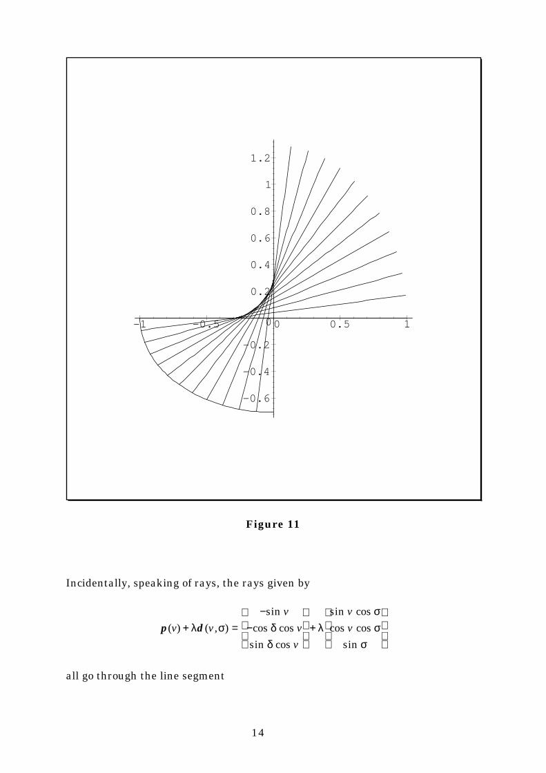
It is also instructive to depict sunrays touching the surface. This can be done bythe Maple commands

> ray:=[p[1]+l*d[1],p[2]+l*d[2],l=0..2]:

ray:=subs(v=k*Pi/24,ray):

rays:=seq(ray,k=0..12):

astroid:=subs(v=l,r[1]),subs(v=l,r[2]):

perimeter:=subs(v=l,p[1]),subs(v=l,p[2]):

>sigma:=0:plot({rays,[astroid,l=0..Pi/2],[perimeter,l=0..Pi/2]});

where σ = 0. The result is Figure 11.

* A classic is the cast iron garden sundial manufactured by the Finnish metal com-pany Valmet decades ago.

** But see Section 6.

8

0

0.2

0.4

0.6

0.8

1

-0.6

-0.4

-0.2

0

0.2

-1-0.8

-0.6-0.4

-0.20

From 12 o’clock to 18 o’clock

Figure 3

9

-0.6

-0.4

-0.2

0

0.2

0.4

0.6

0.8

1

-0.2

0

0.2

0.4

0.6

-1-0.8

-0.6-0.4

-0.20


Figure 4

10

-0.6

-0.4

-0.2

0

0.2

0.4

0.6

0.8

1

-0.2

0

0.2

0.4

0.6

00.2

0.40.6

0.81


Figure 5

11

0

0.2

0.4

0.6

0.8

1

-0.6

-0.4

-0.2

0

0.20

0.20.4

0.60.8

1


Figure 6

12


Figure 7


Figure 8

13


Figure 9


Figure 10

14

-0.6

-0.4

-0.2

0

0.2

0.4

0.6

0.8

1

1.2

-1 -0.5 0 0.5 1

Figure 11

Incidentally, speaking of rays, the rays given by

p d( ) ( )sin

cos cossin cos

sin coscos cos

sin

v vv

vv

vv+ =

−−

+

λ σ δδ

λσσ

σ,

all go through the line segment

15

xy vz v

== −= +

01( cos )cos

sin cos tan

δδ σ

in the yz-plane, corresponding to λ = 1/cos σ. This line segment can then be used

as a gnomon, changes in σ simply raise or lower it without altering its direction.

This observation leads to certain old classical analemmatic sundial constructions,see [Ro].

The four quarters of the sundial can be translated to different positions in a vari-ety of ways, some of them leading to quite pleasing designs. An interesting caseis δ = π/2: the sundial is then totally inside the astroidal cylinder. A horizontal

sundial is obtained by taking δ = 90° – local latitude. And a vertical sundial is

obtained by taking δ = – local latitude (this sundial can be fixed on a south facing

window pane, say).

16

4. The Equation of Time

Solar time is not the time used in everyday activity (except in certain parts of theworld). There are the different time zones and the varying velocity of Earth in itsorbit around Sun and the fact that Earth’s axis is not perpendicular to the planeof ecliptic.

The actual dynamics of Earth in thesolar system is quite complicated. As afirst approximation it might be as-sumed that Kepler’s laws are accurate.An xyz-coordinate system may then beused where the xy-plane is the plane ofecliptic, the point of perigeum being onthe positive x-axis and Sun is in theorigin, see Figure 1 4. The orbit ofEarth is an ellipse with eccentricity ε,

in polar coordinates

Sun

x

y

Earth

rφ

Figure 14

ra= −+( )

cos

11

2εε φ

where a is the length of the major semiaxis. The dynamics is then given by theangular velocity

φ̇

εε φ ε φ= =

−+ = +C

r

C

a K2 2 2 22 2

11

11

( )( cos ) ( cos ) ,

where C is a constant (actually C a GM= −( )1 2ε where M is Sun’s mass and Gis the gravitational constant), once the initial value φ(0) = 0 is given. The con-

stant K can be obtained from the equation

1

1 10

1

20

1

20

2= =

+( )=

+∫ ∫ ∫˙˙

˙φφ

φε φ

φε φ

π( )( )

( )

cos ( ) ( cos )

tt

dt Kt dt

tK

d.

Denote then r = (r cos φ,r sin φ,0) and let a = (a1,a2,a3) be the direction vector of

Earth’s axis where a3 > 0. Solar time is obtained when a constant velocity (thevalue of which is immaterial here) minus the turning velocity of the plane con-taining Earth’s axis and Sun is integrated. This turning velocity ̇θ is the same asthe angular velocity of the vector s = r × a, i.e.,

17

˙ ˙θ =

×s s

s 2 .

Now

( ) ( ) ( ) ( ) ( ) ( )r a r a r a a r r a r a a r r a a k a a× × × = × •( ) − × •( ) = • × = • =˙ ˙ ˙ ˙ C Ca3

( r r k× =˙ C by the conservation of angular momentum or that of areal velocity)and

r a r a r a r a a r a r a a r× = • × × = • • − •( ) = − •2 2 2( ) ( ) ( ) ( )r ,

so

˙˙

θ φ=− •

=− •

Ca

r

a

r

32 2

32

1( )a r

ar

.

If a is written in the form

a = (cos α sin β,sin α sin β,cos β)

then

− = • = + = −sin cos sin sin cos( ) σ φ φ β φ αa

rr

a a1 2

(which gives the relation between declination σ and polar angle φ mentioned in

Section 2 and needed later) and

˙˙

θ β φβ φ α

=− −

(cos )

sin cos ( )

1 2 2 .

The mean solar time is an “artificial” time corresponding to θ̇ π= 2 rad/year. Itclosely approximates the local time one daily uses (correction to a time zone or adaylight savings time is not included, of course).

The difference of mean solar time and solar time is the equation of time*

* Often the equation of time is –E.

18

E dK

dt

t=

− −( )−

=

− −−

+

∫ ∫(cos ) ( )

sin cos ( )

cos

sin cos ( ) ( cos )

β φ τβ φ τ α

π τ ββ ϕ α

πε ϕ

ϕω

φ˙

12

1

2

12 2 2 2 20

where ω is chosen to make E equal to zero at a specified time t0 or polar angle. It

is possible to integrate E by hand but the result involves several branches of arc-tangent and is thus awkward to use.

In order to use the equation of time to map solar time to mean solar time valuesof the eccentricity ε and the angles α and β as well as ω are needed. From [AA]

the following values (valid at January 1st 1995) can be read:

ε = 0.01671043

α = –12.852316° = –0.22431523 rad (mean longitude of winter solstice)

β = 23.439942° = 0.40910416 rad (mean obliquity of ecliptic)

ν = –3.6567940° = –0.06382310 rad (mean New Year)

[AA] also gives the following expression for –E accurate to a few seconds of time:

–E = –106.6 sin L + 596.1 sin(2L) + 4.4 sin(3L) – 12.7 sin(4L)– 428.8 cos L – 2.1 cos(2L) + 19.3 cos(3L)

where

L = 279.196° + 0.985647°d = 4.87289 + 0.0172028d rad

and d is the day of the year. Maple can be used to solve for a day d0 when E = 0:

> L:=4.87289+0.0172028*d:

> fsolve(-106.6*sin(L)+596.1*sin(2*L)+4.4*sin(3*L)-12.7*sin(4*L)

-428.8*cos(L)-2.1*cos(2*L)+19.3*cos(3*L),d);

-5.529862392

Thus d0 = –5.5298624.

To plot and investigate the equation of time Matlab is used because of the exten-sive numerical calculations needed. First, values of constants are given in Con-stants.m:

% Constants

19

global alpha beta omega delta epsilon zeta axdir K nu t0

alpha=-0.22431523;

beta=0.40910416;

nu=-0.06382310;

t0=-5.529862392/365.242190;

delta=0;

epsilon=0.01671043;

zeta=0;

K=1/quad('AngVel',0,2*pi);

omega=fzero('OmegaEq',nu);

axdir=[cos(alpha)*sin(beta) sin(alpha)*sin(beta) cos(beta)];

(values of ζ other than 0 will be needed in Section 6). The length of year is

365.242190 days, the tropical year of 1995. The equation giving time t (in years)in terms of the polar angle φ is

t Kd

t

=+∫ φ

ε φν

φ

( cos )

( )

1 2 ,

hence the Matlab-functions

function y=AngVel(f)

global epsilon

y=1 ./(1+epsilon*cos(f)).̂ 2;

and

function y=OmegaEq(a)

global t0 K nu

y=K*quad('AngVel',a,nu)+t0;

The equation of time (E vs. φ) is then given by

20

function y=TimEqMin(phi)

global omega zeta

y=(zeta+quad('TimEqD',omega,phi))/2/pi*24*60;

where

function y=TimEqD(phi)

global axdir K epsilon

y=axdir(3)./(1-(axdir(1)*cos(phi)+axdir(2)*sin(phi)).̂ 2)- ...

2*pi*K./(1+epsilon*cos(phi)).̂ 2;

The plot of this function is Figure 15 below.

0 1 2 3 4 5 6-20

-15

-10

-5

0

5

10

15

Figure 15

The equation of time in [AA] is plotted below, first E vs. d and then E vs. φ.

21

0 50 100 150 200 250 300 350-20

-15

-10

-5

0

5

10

15

Figure 16

0 1 2 3 4 5 6-20

-15

-10

-5

0

5

10

15

Figure 17

22

As is seen, Figures 15 and 17 are very close. The difference is plotted in secondsin Figure 18.

0 1 2 3 4 5 6-8

-7

-6

-5

-4

-3

-2

-1

0

1

Figure 18

Thus the two equations of time are in agreement within about 7.5 seconds oftime. Interestingly there appears to be a systematic difference of about –3 sec-onds (plus other low frequency components). This is probably an artifact of forc-ing the equation of time to be zero near New Year at the same time as that of[AA].

A more exact modelling of Earth’s dynamics is beyond the scope of this paper, aninterested reader is referred to the excellent presentation of this subject matterin [Se]. The effects of other planets and Moon should be included as well as cer-tain relativistic effects. It should also be noted that Earth’s axis precesses andnutates. Indeed, the exact values of α and β slowly change, the formulas given in

[AA] for the year 1995 are

α = –12.852316 + 0.00004707d,

β = 23.439942 – 0.00000036d

23

where d is the day of the year. The very ecliptic slowly changes, e.g. the exactvalue of ε in [AA] for 1995 is

ε = 0.01671043 – 0.0000000012d.

In the sequel the integral form of E is used, even though the approximative trig-onometric form given in [AA] may be more accurate (and certainly numericallyfaster). This E is within some ±10 seconds of time from the correct value, andlikely even more accurate. The accuracy is quite sufficient, it should be notedthat some famous sundial constructs were made using a much more crude equa-tion of time, c.f. e.g. [Lo]. On the other hand, there might be an advantage inhaving a formula modelling E, not just an approximate formula.

24

5. An Equatorial Mean Solar Time Sundial

The idea behind designing a mean solar time dundial is to express a ray fromSun to the point p(w) on the perimeter of the sundial in the form

p(w) + λd(v,φ)

where φ is Earth’s polar angle, cf. Section 2. The connection between Sun’s decli-

nation σ and its polar angle φ was obtained in the previous section:

sin cos sin sin cos( ) σ φ φ β φ α= − − = − −a a1 2 .

Thus σ is uniquely determined by φ, this dependence is shown in the plot of σ vs.

φ (by Maple) below.

-0.4-0.200.20.4

0 1 2 3 4 5 6phi

Figure 19

So

d( )

sin cos

cos cos

sin

sin sin cos ( )

cos sin cos ( )

sin cos( )

v

v

v

v

v,φ

σ

σ

σ

β φ α

β φ α

β φ α

=

=

− −

− −

− −

1

1

2 2

2 2 .

Further, setting the normal of the shadow casting surface perpendicular tod(v,φ), one gets

25

λ φ φ

φ=

′ × − •× •

p d d dd d d

( )w wv v

v

where

dv

v

v=

− −

− − −

cos sin cos ( )

sin sin cos ( )

1

1

0

2 2

2 2

β φ α

β φ α and

dφ

β φ α φ α

β φ αβ φ α φ α

β φ αβ φ α

=

− −

− −− −

− −−

sin sin cos( )sin( )

sin cos ( )

cos sin cos( )sin( )

sin cos ( )sin sin( )

v

v

2

2 2

2

2 2

1

1.

For a mean solar time sundial

w = v + E(φ)

and so the shadow caster surface is given by

r(v,φ) = p(v + E(φ)) + λ(v,φ)d(v,φ)

where

λ φ

φ=

′ × ′ − •× •

p d d dd d d( )E v

v

and

′ =− −

−+

EK

( )cos

sin cos ( ) ( cos )

φ β

β ϕ απ

ε ϕ1

2

12 2 2 .

It should be noted first that the expanded form of r(v,φ) (even without the formu-

las for E and E′) is quite formidable, as the reader may verify by expanding it

with Maple. The ruled surface generated by the sunrays for any specific value ofv can however be plotted by Matlab quite speedily. For v = 0 it is the surfacegiven by

r0(λ,φ) = p(E(φ)) + λd(0,φ).

Figure 20 is plotted by

26

% SunRays

global alpha delta X Y Z

Constants

delta=pi/4;

lambdalow=0;

lambdaup=3;

philow=alpha;

phiup=2*pi+alpha;

nods=30;

X=zeros(nods+1);

Y=zeros(nods+1);

Z=zeros(nods+1);

for n=0:nods

phi=philow+n*(phiup-philow)/nods;

TimErr=TimEq(phi);

for m=0:nods

lambda=lambdalow+m*(lambdaup-lambdalow)/nods;

r=Time(0,TimErr)+lambda*DirTan(0,phi);

X(n+1,m+1)=r(1);

Y(n+1,m+1)=r(2);

Z(n+1,m+1)=r(3);

end

end

view([1 3 1])

axis([-1 1 -1 1 -1 1])

mesh(X,Y,Z)

where

function y=Time(v,terror)

global delta

27

y=[-sin(v+terror) -cos(delta)*cos(v+terror) sin(delta)*cos(v+terror)];

and

function y=DirTan(v,phi)

global alpha beta

y=[sin(v)*sqrt(1-sin(beta)̂ 2*cos(alpha-phi)̂ 2) ...

cos(v)*sqrt(1-sin(beta)̂ 2*cos(alpha-phi)̂ 2) -sin(beta)*cos(alpha-phi)];

-1-0.500.51

-1

-0.5

0

0.5

1

-1

-0.5

0

0.5

1

Figure 20

The cross section of the surface in Figure 20 shows the ubiquitous unsymmetricform of the “figure of eight” or the analemmic figure. It can be read from Figure20 that the shadow caster surface must be constructed from two parts, one forα ≤ φ ≤ π + α (the “spring part”) and the other for π + α ≤ φ ≤ 2π + α (the “autumn

part”), otherwise any point of the surface is almost always covered from Sun bysome other part of the surface and there cannot be a shadow!

28

A serious difficulty presents itself at this point, although it is not apparent inFigure 20: All components of dφ contain the factor sin(φ – α) and thus dφ = 0 and

dv × dφ • d = 0 when φ = α or φ = π + α . (Actually these are the only values of φwhich make dv × dφ • d equal to zero.) Thus there is a singularity when φ = α or

φ = π + α . Indeed, the shadow caster surface is unbounded and parts of it are not

realistic in that they correspond to negative values of λ. This difficulty must be

addressed and avoided as far as possible.

The purpose of this section is to design an equatorial sundial, i.e., here δ = 0.

Thus

p( )sincos

sin ( )cos ( )

www

v Ev E=

−−

=− +− +

( )( )

0 0

φφ and ′ =

−

=− +

+

( )( )p ( )

cossin

cos ( )sin ( )

ww

wv E

v E0 0

φφ .

It is immediately verified that now application of the rotation matrix

cos sinsin cos

ν νν ν

00

0 0 1−

to each of the vectors p,p′,d,dv and dφ simply adds ν to the value of v. Since the

values of the triple products p′ × (E′dv – dφ) • d and dv × dφ • d are not changed

by rotations, it follows that the surface given by

r(v,φ) = p(v + E(φ)) + λ(v,φ)d(v,φ)

is a surface of revolution with z-axis as its axis of revolution.

The only way to counter the effect of the numerator of λ being zero when φ = α or

φ = π + α is to make the denominator simultaneously zero (preferably with the

same order although this is not stressed here). Now, if dφ = 0, then

p′ × (E′dv – dφ) • d = 0

if E′ = 0. However, from Figure 15 it is seen that this is not a usable option, the

values of φ making E′ zero are too far from α and π + α . On the other hand, the

vectors p′ and dv are linearly dependent when E = 0. Using this possibility is

tantamount to choosing the value of ω to satisfy E(α ) = 0 or E(π + α) = 0. This is

a viable option since the dates of winter and summer solstices are not too far

29

from zeros of the equation of time. In fact, ω can be made to slowly change with φto satisfy both of these equations, a construct used later.

To see how severe an effect the “blow-up” near the values φ = α and φ = π + α will

have, the surface or its profile can be plotted. Matlab is used because of theamount of numerical computation. The profile of the shadow caster surface in theinterval α + 0.001 ≤ φ ≤ π + α – 0.001 (spring) is obtained by

% ArmillaryProfile

global alpha delta zeta

Constants

delta=0;

v=0;

zeta=0;

philow=alpha+0.001;

phiup=pi+alpha-0.001;

nods=100;

R=zeros(nods+1,1);

Z=zeros(nods+1,1);

for n=0:nods


TimErr=TimEq(phi);

TimErrD=TimEqD(phi);

distance=dot(cross(TimeD(v,TimErr),TimErrD*DirTanDv(v,phi)- ...

DirTanDphi(v,phi)),DirTan(v,phi))/ ...

dot(cross(DirTanDv(v,phi), ...

DirTanDphi(v,phi)),DirTan(v,phi));

r=Time(v,TimErr)+distance*DirTan(v,phi);

R(n+1,1)=sqrt(r(1)̂ 2+r(2)̂ 2);

Z(n+1,1)=r(3);

end

plot(R,Z)

axis('equal')

hold

30

plot(-R,Z)

hold

where p′ is given by

function y=TimeD(v,terror)

global delta

y=[-cos(v+terror) cos(delta)*sin(v+terror) -sin(delta)*sin(v+terror)];

and dφ and dv by

function y=DirTanDphi(v,phi)

global alpha beta

y=[sin(v)*sin(beta)̂ 2*cos(phi-alpha)*sin(phi-alpha)/ ...

sqrt(1-sin(beta)̂ 2*cos(phi-alpha)̂ 2) ...

cos(v)*sin(beta)̂ 2*cos(phi-alpha)*sin(phi-alpha)/ ...

sqrt(1-sin(beta)̂ 2*cos(phi-alpha)̂ 2) sin(beta)*sin(phi-alpha)];

and

function y=DirTanDv(v,phi)

global alpha beta

y=[cos(v)*sqrt(1-sin(beta)̂ 2*cos(phi-alpha)̂ 2) ...

-sin(v)*sqrt(1-sin(beta)̂ 2*cos(phi-alpha)̂ 2) 0];

The resulting plot is in Figure 21. The “explosion” is clearly seen but it is notvery serious because the angle 0.001 radians is about 1.4 h of time. It is well pos-sible to choose a much larger angle and still obtain a reasonably small period of

31

-0.8 -0.6 -0.4 -0.2 0 0.2 0.4 0.6 0.8

-0.6

-0.4

-0.2

0

0.2

0.4

Figure 21

-0.4 -0.2 0 0.2 0.4

-0.4

-0.3

-0.2

-0.1

0

0.1

0.2

0.3

0.4

Figure 22

32

unavailability. For instance letting φ be in the interval α + 0.03 ≤ φ ≤ π + α – 0.03

gives Figure 22. There the explosion is much less pronounced and can be seenclearly only in an enlargement (Figures 23 and 24). The angle 0.03 correspondsto about 1.7 days, so the total time of unavailability is about a week. In Finlandthis is of no consequence in winter and might be considered as acceptable.

The shape of the shadow caster surface is different in autumn. Plotting for thevalues π + α + 0.001 ≤ φ ≤ 2π + α – 0.001 gives Figure 25. Again choosing the in-

terval π + α + 0.03 ≤ φ ≤ 2π + α – 0.03 nearly disposes of the “explosive” parts

(Figure 26) (but not quite, as could be seen in enlarged pictures).

There are thus two problems: First, getting rid of the “explosive” parts of the sur-faces, and second, the fact that two surfaces are needed, one for spring and theother for autumn. Making the surfaces removable may lead to some rather cum-bersome arrangements, note that both surfaces taper to a point. One possibilityis to cut the profiles in thin sheets and position them perpendicular to each otherwith z-axis as the line of intersection. The proper profile is then turned to facethe sun (the other profile can be used to do this as its shadow will disappear inthe correct position).

-0.1 -0.05 0 0.05 0.10.22

0.24

0.26

0.28

0.3

0.32

0.34

0.36

0.38

0.4

0.42

Figure 23

33

-0.1 -0.05 0 0.05 0.1 0.15

-0.42

-0.4

-0.38

-0.36

-0.34

-0.32

-0.3

-0.28

-0.26

-0.24

Figure 24

-0.6 -0.4 -0.2 0 0.2 0.4 0.6-0.6

-0.4

-0.2

0

0.2

0.4

0.6

Figure 25

34

-0.4 -0.2 0 0.2 0.4

-0.4

-0.3

-0.2

-0.1

0

0.1

0.2

0.3

0.4

Figure 26

Plotting the two surfaces reveals the lines of constant v and φ. Since these sur-

faces are surfaces of revolution, the lines of constant φ are circles. It should be

noted that as φ changes, only one point in each of these circles may serve as the

touching point of a sunray giving time on the dial during a day. The lines of con-stant v are spirals of small torsion.

The “spring” surface (α + 0.03 ≤ φ ≤ π + α – 0.03) is plotted by

% Armillary

global alpha delta zeta X Y Z

Constants

delta=0;

zeta=0;

vlow=0;

vup=2*pi;

philow=alpha+0.03;

35


nods=30;

X=zeros(nods+1);

Y=zeros(nods+1);

Z=zeros(nods+1);

for n=0:nods


TimErr=TimEq(phi);


for m=0:nods

v=vlow+m*(vup-vlow)/nods;






X(n+1,m+1)=r(1);

Y(n+1,m+1)=r(2);

Z(n+1,m+1)=r(3);

end

end

mesh(X,Y,Z)

view([1 1 0.5])

axis([-0.1 0.1 -0.1 0.1 -0.5 0.5])

The result is in Figure 27. The “autumn” surface is obtained by letting φ range in

the interval π + α + 0.03 ≤ φ ≤ 2π + α – 0.03 (Figure 28). The locus of the touching

points of sunrays on the shadow casting surface is a tightly woven spiral. Thisspiral can be plotted by

% ArmillarySpiral

global alpha delta zeta

Constants

36

-0.1-0.05

00.05

0.1

-0.1-0.05

00.05

0.1

-0.5

0

0.5

Figure 27

37

-0.1-0.05

00.05

0.1

-0.1-0.05

00.05

0.1

-0.5

0

0.5

Figure 28

38

delta=0;

zeta=0;

philow=alpha+0.03;


nods=1000;

X=zeros(nods+1,1);

Y=zeros(nods+1,1);

Z=zeros(nods+1,1);

for n=0:nods


TimErr=TimEq(phi);


v=K*quad('AngVel',nu,phi)*365.242192*2*pi;






X(n+1)=r(1);

Y(n+1)=r(2);

Z(n+1)=r(3);

end

plot3(X,Y,Z)

view([1 1 0.5])

axis([-0.1 0.1 -0.1 0.1 -0.5 0.5])

The results are in Figure 29 (spring)and Figure 30 (autumn).

As indicated above, a way to remove the effect of the “blow-up” near φ = α and

φ = π + α is to make the equation of time zero for these values of φ. This of course

sacrifices some accuracy. Now, one way to define such an equation of time is todefine

E

KdSpring ( ) ( )

cos

sin cos ( ) ( cos )

φ τ

πφ α β

β ϕ απ

ε ϕϕ

α

φ= − +

− −−

+

∫ 1

2

12 2 2

39

-0.1-0.05

00.05

0.1

-0.1-0.05

00.05

0.1

-0.5

0

0.5

Figure 29

40

-0.1-0.05

00.05

0.1

-0.1-0.05

00.05

0.1

-0.5

0

0.5

Figure 30

and

41

E

KdAutumn( ) ( )

cos

sin cos ( ) ( cos )

φ τ

ππ α φ β

β ϕ απ

ε ϕϕ

α

φ= + − +

− −−

+

∫21

2

12 2 2

where

τ ββ ϕ α

πε ϕ

ϕα

α π= −

− −−

+

+

∫ cos

sin cos ( ) ( cos )

1

2

12 2 2K

d = –0.01486978.

Then

ESpring(α) = ESpring(π + α) = 0,

EAutumn(α + π) = EAutumn(2π + α) = 0.

The former is plotted in the interval α + 10–10 ≤ φ ≤ π + α – 10–10 by

% ArmillarySpringPr

global alpha delta tau

Constants

delta=0;

v=0;

tau=-quad('TimEqD',alpha,pi+alpha);

philow=alpha+1.e-10;

phiup=pi+alpha-1.e-10;

nods=100;

R=zeros(nods+1,1);

Z=zeros(nods+1,1);

for n=0:nods


TimErr=TimEqSpring(phi);

TimErrD=tau/pi+TimEqD(phi);



42




R(n+1,1)=sqrt(r(1)̂ 2+r(2)̂ 2);

Z(n+1,1)=r(3);

end

plot(R,Z)

axis('equal')

hold

plot(-R,Z)

hold

where ESpring is given by

function y=TimEqSpring(phi)

global alpha tau

y=tau/pi*(phi-alpha)+quad('TimEqD',alpha,phi);

The latter is plotted in the interval π + α + 10–10 ≤ φ ≤ 2π + α – 10–5 by

% ArmillaryAutumnPr

global alpha delta tau

Constants

delta=0;

v=0;

tau=-quad('TimEqD',alpha,pi+alpha);

philow=pi+alpha+1.e-10;

phiup=2*pi+alpha-1.e-5;

nods=100;

R=zeros(nods+1,1);

Z=zeros(nods+1,1);

for n=0:nods

43


TimErr=TimEqAutumn(phi);

TimErrD=-tau/pi+TimEqD(phi);


DirTanDphi(dial,phi)),DirTan(dial,phi))/ ...




R(n+1,1)=sqrt(r(1)̂ 2+r(2)̂ 2);

Z(n+1,1)=r(3);

end

plot(R,Z)

axis('equal')

hold

plot(-R,Z)

hold

where EAutumn is given by

function y=TimEqAutumn(phi)

global alpha tau

y=tau/pi*(2*pi+alpha-phi)+quad('TimEqD',alpha,phi);

The resulting plots are Figures 31 and 32, respectively.

44

-0.4 -0.2 0 0.2 0.4

-0.4

-0.3

-0.2

-0.1

0

0.1

0.2

0.3

0.4

Figure 31

-0.4 -0.2 0 0.2 0.4

-0.4

-0.3

-0.2

-0.1

0

0.1

0.2

0.3

0.4

Figure 32

45

As can be seen, these profiles are rather similar, which suggests that

EAutumn(2π + 2α – φ) ≅ –ESpring(φ) for α ≤ φ ≤ π + α .

Indeed, plotting EAutumn(2π + 2α – φ) + ESpring(φ) in seconds of time gives Figure

33 and shows that the difference is at most some 45 seconds of time.

0 0.5 1 1.5 2 2.5-50

-40

-30

-20

-10

0

10

20

30

40

50

Figure 33

Thus, both the effect of the “blow-up” and the problem of having two shadowcaster surfaces are removed if the equation of time given by

E E ECommon Spring Autumn( ) ( ) ( )φ φ π α φ= − + −( )1

22 2

is used. The plot of this equation of time in minutes of time is in Figure 34. Thedifference E(φ) – ECommon(φ) is plotted in Figure 35. It can be seen that there is

considerable loss of accuracy, an accuracy of some ±115 seconds of time is, how-ever, achieved. Since

46

0 1 2 3 4 5 6-20

-15

-10

-5

0

5

10

15

20

Figure 34

0 1 2 3 4 5 6-2

-1.5

-1

-0.5

0

0.5

1

1.5

2

Figure 35

47

ESpring(φ) + ESpring(2π + 2α – φ) = EAutumn(φ) + EAutumn(2π + 2α – φ)

it follows that

ECommon(2π + 2α – φ) = –ECommon(φ),

i.e., ECommon is antisymmetric about φ = π + α, and only one shadow caster sur-

face is needed, as told. A calculation shows that

E

K KdCommon( )

cos

sin cos ( ) ( cos ) cos ( )

φ β

β ϕ απ

ε ϕπ

ε ϕ αϕ

α

φ=

− −−

+−

+ −( )

∫ 1 1 1 22 2 2 2

so the numerical values of ECommon are obtained by

function y=TimEqCommon(phi)

global alpha

y=quad('TimEqCommonD',alpha,phi);

where ′ECommon is given by

function y=TimEqCommonD(phi)

global alpha axdir K epsilon

y=axdir(3)./(1-(axdir(1)*cos(phi)+axdir(2)*sin(phi)).̂ 2)- ...

pi*K./(1+epsilon*cos(phi)).̂ 2-pi*K./(1+epsilon*cos(phi-2*alpha)).̂ 2;

The profile of the shadow caster surface corresponding to ECommon can be plottedby

% ArmillaryCommonPr

global alpha delta

Constants

delta=0;

48

v=0;

philow=alpha+1.e-5;


nods=100;

R=zeros(nods+1,1);

Z=zeros(nods+1,1);

for n=0:nods


TimErr=TimEqCommon(phi);

TimErrD=TimEqCommonD(phi);






R(n+1,1)=sqrt(r(1)̂ 2+r(2)̂ 2);

Z(n+1,1)=r(3);

end

plot(R,Z)

axis('equal')

hold

plot(-R,Z)

hold

The plot is in Figure 36. The surface itself can be plotted by

% ArmillaryCommon

global alpha delta

Constants

delta=0;

vlow=0;

vup=2*pi;

49

philow=alpha+1.e-10;


nods=30;

X=zeros(nods+1);

Y=zeros(nods+1);

Z=zeros(nods+1);

for n=0:nods


TimErr=TimEqCommon(phi);

TimErrD=TimEqCommonD(phi);

for m=0:nods


-0.4 -0.2 0 0.2 0.4

-0.4

-0.3

-0.2

-0.1

0

0.1

0.2

0.3

0.4

Figure 36

50

-0.1-0.05

00.05

0.1

-0.1-0.05

00.05

0.1

-0.5

0

0.5

Figure 37

51






X(n+1,m+1)=r(1);

Y(n+1,m+1)=r(2);

Z(n+1,m+1)=r(3);

end

end

mesh(X,Y,Z)

view([1 1 0.5])

axis([-0.1 0.1 -0.1 0.1 -0.5 0.5])

The resulting plot is in Figure 37.

52

6. Timeshifts

It may be necessary to show a shifted time to compensate for the difference be-tween local time or, say, daylight savings time. Suppose a timeshift of ζ is

required. There are three methods of achieving this:

(1)

(2)

(3)

Rotate the face of the sundial anticlockwise by ζ. (This works because ofthe equal-hour scale used throughout.)Rotate the whole assembly (the face of the sundial + the shadow castersurface) around the z-axis by the angle ζ.Construct a new shadow caster surface corresponding to w = v + ζ.

Methods 1 and 2 are very easily implemented, so there would not appear to beany need for both of them or for Method 3. However, one can apply one of themethods and then compensate the effect using the other methods. In this way alot of new sundial designs are obtained.

For example, using Method 2 to rotate the sundial to the desired position, the re-sulting error in time can be corrected by using Method 1. The unit normal of theface of the sundial is then

cos sin 0

sin cos 0

0 0 1

cos sin

sin cos

sin sin

cos sin

cos

ζ ζζ ζ δ δ

δ δ

ζ δζ δ

δ

−

−

=−

1 0 0

0

0

0

0

1

.

Thus an east-west sundial can be obtained by choosing δ = π/2 and ζ = π/2 (a six

hour timeshift).

In what follows, Method 3 is used (and the correction is made by Method 1, say).First, the solar time sundial of Section 3 is considered. Maple can be used tocompute the parametric representation of the shadow caster surface, exactly asin Section 3:

> with(linalg):

Warning: new definition for norm

Warning: new definition for trace

_

> p:=[-sin(v+zeta),-cos(delta)*cos(v+zeta),sin(delta)*cos(v+zeta)]:

_

> d:=[sin(v)*cos(sigma),cos(v)*cos(sigma),sin(sigma)]:

_

> lambda:=evalm(-dotprod(crossprod(diff(p,v),diff(d,sigma)),d))/

53

dotprod(crossprod(diff(d,v),diff(d,sigma)),d);

lambda := (- (cos(delta) sin(v + zeta) cos(sigma)

- sin(delta) sin(v + zeta) cos(v) sin(sigma)) sin(v) cos(sigma) -

(sin(delta) sin(v + zeta) sin(v) sin(sigma) + cos(v + zeta) cos(sigma))

cos(v) cos(sigma) - (cos(v + zeta) cos(v) sin(sigma)

/

+ cos(delta) sin(v + zeta) sin(v) sin(sigma)) sin(sigma)) / (

/

2 3 2 3

- sin(v) cos(sigma) - cos(v) cos(sigma) +

2 2

(- cos(v) cos(sigma) sin(sigma) - sin(v) cos(sigma) sin(sigma))

sin(sigma))

_

> lambda:=simplify(");

sin(v) cos(delta) sin(v + zeta) + cos(v) cos(v + zeta)

lambda := ------------------------------------------------------

cos(sigma)

_

> r:=evalm(p+lambda*d);

r := [ - sin(v + zeta) + %1 sin(v),

- cos(delta) cos(v + zeta) + %1 cos(v),

%1 sin(sigma)

sin(delta) cos(v + zeta) + ------------- ]

cos(sigma)

%1 := sin(v) cos(delta) sin(v + zeta) + cos(v) cos(v + zeta)

The shadow caster surface has then the parametric representation

x v v v v v vy v v v v v vz z

= − + + + + += − + + + + +=

sin( ) cos sin sin( ) sin cos cos( )cos cos( ) cos sin cos sin( ) cos cos( )

ζ δ ζ ζδ ζ δ ζ ζ

2

2

.

54

This is a cylindrical surface with z-axis as its axis. For instance, for δ = 0 the

cylinder is circular with radius |sin ζ|. An animation showing how the curve

(x,y) changes when ζ ranges in [0,π/2] (and δ = π/4) is obtained by

> delta:=Pi/4:with(plots):

_

> animate([r[1],r[2],v=0..2*Pi],zeta=0..Pi/2,numpoints=50,frames=20);

It shows that for a large enough |ζ| this curve is smooth and encloses a convex

area. Indeed, for ζ = π/2 this curve is as shown in Figure 38.

-0.6

-0.4

-0.20

0.2

0.4

0.6

-1 -0.5 0 0.5 1

zeta = 6 h

Figure 38

To obtain the break point value of ζ the tangent of the curve is calculated:

> diff([r[1],r[2]],v);

[- cos(v + zeta) + (cos(v) cos(delta) sin(v + zeta)

+ sin(v) cos(delta) cos(v + zeta) - sin(v) cos(v + zeta)

55

- cos(v) sin(v + zeta)) sin(v)

+ (sin(v) cos(delta) sin(v + zeta) + cos(v) cos(v + zeta)) cos(v),

cos(delta) sin(v + zeta) + (cos(v) cos(delta) sin(v + zeta)

+ sin(v) cos(delta) cos(v + zeta) - sin(v) cos(v + zeta)

- cos(v) sin(v + zeta)) cos(v)

- (sin(v) cos(delta) sin(v + zeta) + cos(v) cos(v + zeta)) sin(v)

]

_

> map(simplify,");

[- 2 cos(v + zeta) + 2 sin(v) cos(v) cos(delta) sin(v + zeta)

2

+ cos(delta) cos(v + zeta) - cos(delta) cos(v + zeta) cos(v)

2

+ 2 cos(v) cos(v + zeta) - sin(v) cos(v) sin(v + zeta),

2

2 cos(v) cos(delta) sin(v + zeta)

+ cos(v) sin(v) cos(delta) cos(v + zeta)

2

- 2 cos(v) sin(v) cos(v + zeta) - cos(v) sin(v + zeta)]

Thus

′ = − + + − +( )′ = − + + − +( )

x v v v v v vy v v v v v v

( ) sin (cos )sin cos( ) ( cos )cos sin( )( ) cos (cos )sin cos( ) ( cos )cos sin( )

δ ζ δ ζδ ζ δ ζ

2 2 12 2 1 .

The breakpoint is thus determined by the solvability of the equation

(cos δ – 2)sin v cos(v + ζ) + (2 cos δ –1)cos v sin(v + ζ) = 0,

that is,

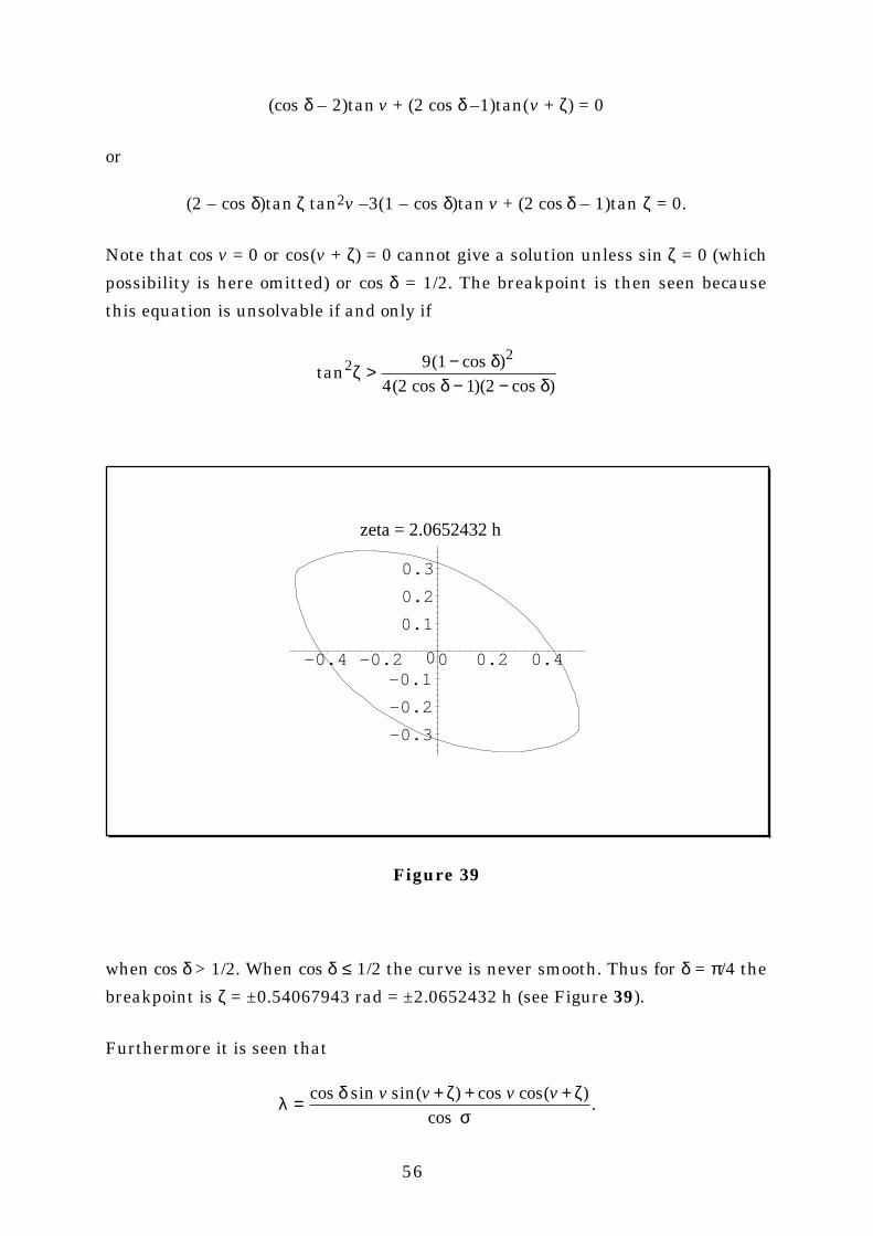
56

(cos δ – 2)tan v + (2 cos δ –1)tan(v + ζ) = 0

or

(2 – cos δ)tan ζ tan2v –3(1 – cos δ)tan v + (2 cos δ – 1)tan ζ = 0.

Note that cos v = 0 or cos(v + ζ) = 0 cannot give a solution unless sin ζ = 0 (which

possibility is here omitted) or cos δ = 1/2. The breakpoint is then seen because

this equation is unsolvable if and only if

tan

( cos )( cos )( cos )

229 1

4 2 1 2ζ δ

δ δ> −

− −

-0.3

-0.2

-0.10

0.1

0.2

0.3

-0.4 -0.2 0 0.2 0.4

zeta = 2.0652432 h

Figure 39

when cos δ > 1/2. When cos δ ≤ 1/2 the curve is never smooth. Thus for δ = π/4 the

breakpoint is ζ = ±0.54067943 rad = ±2.0652432 h (see Figure 39).

Furthermore it is seen that

λ δ ζ ζ

σ= + + +cos sin sin( ) cos cos( )

cos

v v v v

.

57

When there is no timeshift any value of δ in the interval [–π/2,π/2] can be chosen

without making λ negative. For δ = 0 any value of ζ in the interval –π/2 ≤ ζ ≤ π/2

can be chosen as then λ ζ σ= ≥cos cos 0. For δ 0 the equation

cos δ = –cot v cot(v + ζ)

defines the smallest value of δ which makes λ zero. The solutions are “some-

where near” the values v = ±π/2,±3π/2 and correspond to (local) extrema of the

function –cot v cot(v + ζ), plotted by Maple in Figure 40 for ζ = π/4.

-10

-5

0

5

10

-3 -2 -1 0 1 2 3v

zeta = Pi/4 rad

Figure 40

The extrema are easily found. The minimum value is cot2

2ζ which is not less

than 1 in the interval –π/2 ≤ ζ ≤ π/2. The maximum value is tan2

2ζ and so a

proper range for δ is given by

cos tanδ ζ≥ 22

.

58

The conclusion is that it is possible to get a shadow caster surface which need notbe divided into separate parts, provided that the timeshift ζ can be chosen from

the interval

arctan( cos )

2 (2 cos )( cos )arctan cos

3 11 2

2−− −

≤ ≤δδ δ

ζ δ .

The trick is to use Method 3 and then correct using Method 1. The endpoints ofthe interval vs. δ are depicted (by Maple) in Figure 41. Thus this figure gives the

region of proper pairs (δ,ζ).

0

0.2

0.4

0.6

0.8

1

1.2

1.4

1.6

zeta

-1 -0.5 0 0.5 1delta

Figure 41

The points (±δ0,ζ0) of intersection can be found by Maple

> delta0:=fsolve(2*arctan(sqrt(cos(delta)))=arctan(3*(1-cos(delta))/2/

sqrt((2*cos(delta)-1)*(2-cos(delta)))),delta=0..2);

delta0 := 1.024537832

_

59

> zeta0:=evalf(subs(delta=delta0,2*arctan(sqrt(cos(delta)))));

zeta0 := 1.249045772

Note that δ0 is only slightly less than π/3 = 1.047197551. For –δ0 ≤ δ ≤ δ0 the

value ζ = ζ0 is always allowed.

For the equatorial sundial design in Section 5 adopting timeshifts has the effectof aggravating the problems: The “explosive behaviour” near the values φ = α and

φ = π + α becomes more pronounced, as does the difference between the “spring”

surface and the “autumn” surface. These designs appear to have been used, how-ever, see e.g. [Ro], and so they are treated here. Take for instance ζ = π/12

(= 1 h). This is set for Matlab in Constants.m (see Section 4). The resultingspring surface profile (with α + 0.1 ≤ φ ≤ π + α – 0.05) can be plotted by

% GnomonProfile

global alpha delta

Constants

delta=0;

v=0;

philow=alpha+0.1;


nods=100;

R=zeros(nods+1,1);

Z=zeros(nods+1,1);

for n=0:nods


TimErr=TimEq(phi);






60


R(n+1,1)=sqrt(r(1)̂ 2+r(2)̂ 2);

Z(n+1,1)=r(3);

end

plot(R,Z)

axis('equal')

hold

plot(-R,Z)

hold

The result is in Figure 42 and the autumn surface profile (with π + α + 0.05 ≤ φ ≤2π + α – 0.1) is in Figure 43.

-0.4 -0.2 0 0.2 0.4

-0.2

0

0.2

0.4

Figure 42

61

-0.4 -0.2 0 0.2 0.4

-0.4

-0.2

0

0.2

Figure 43

The surfaces (Figures 44 and 45) can be plotted by

% Gnomon

global alpha delta

Constants

delta=0;

vlow=0;

vup=2*pi;

philow=alpha+0.1;


nods=30;

X=zeros(nods+1);

Y=zeros(nods+1);

62

Z=zeros(nods+1);

for n=0:nods


TimErr=TimEq(phi);


for m=0:nods







X(n+1,m+1)=r(1);

Y(n+1,m+1)=r(2);

Z(n+1,m+1)=r(3);

end

end

mesh(X,Y,Z)

view([1 1 0.5])

axis([-0.5 0.5 -0.5 0.5 -0.5 0.5])

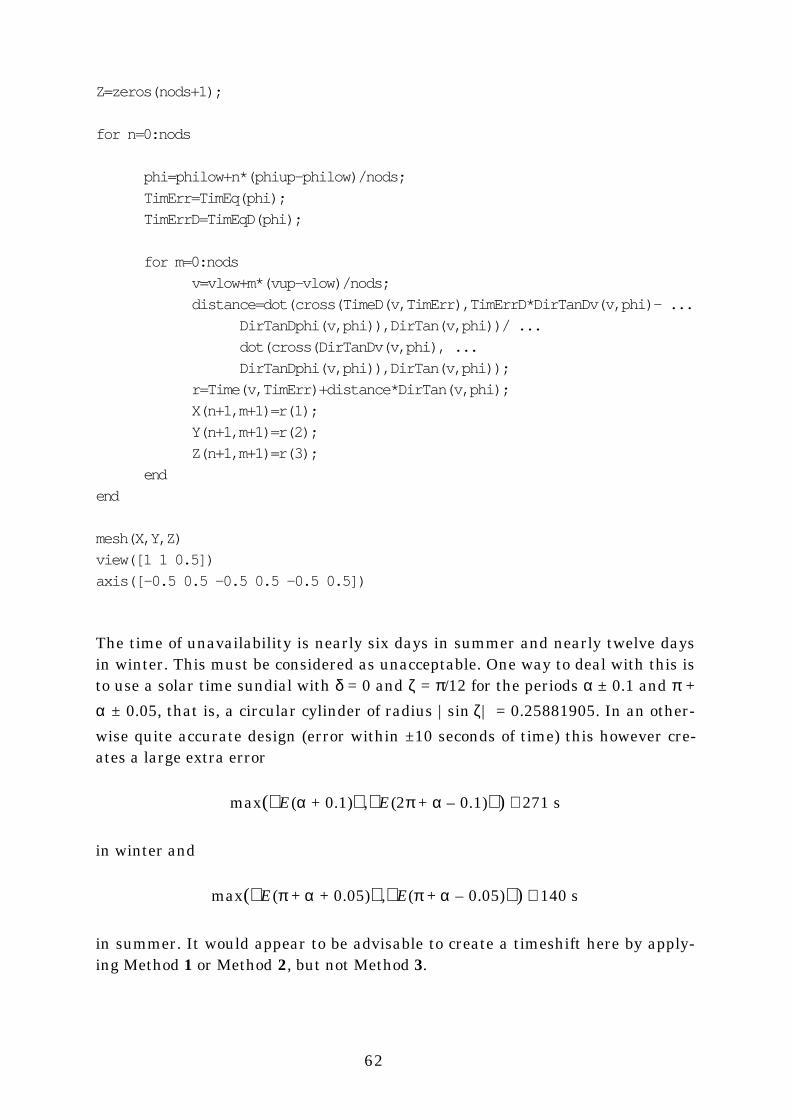
The time of unavailability is nearly six days in summer and nearly twelve daysin winter. This must be considered as unacceptable. One way to deal with this isto use a solar time sundial with δ = 0 and ζ = π/12 for the periods α ± 0.1 and π +

α ± 0.05, that is, a circular cylinder of radius |sin ζ| = 0.25881905. In an other-

wise quite accurate design (error within ±10 seconds of time) this however cre-ates a large extra error

max( E(α + 0.1) , E(2π + α – 0.1) ) ≅ 271 s

in winter and

max( E(π + α + 0.05) , E(π + α – 0.05) ) ≅ 140 s

in summer. It would appear to be advisable to create a timeshift here by apply-ing Method 1 or Method 2, but not Method 3.

63

-0.5

0

0.5

-0.5

0

0.5

-0.5

0

0.5

Figure 44

-0.5

0

0.5

-0.5

0

0.5

-0.5

0

0.5

Figure 45

64

7. A Nonequatorial Mean Solar Time Sundial

For a nonequatorial sundial δ 0. A construct such as in Section 5 may be at-

tempted but the resulting shadow caster surface is quite complicated. Altogethereigth surfaces are needed (assuming that there is no timeshift) corresponding tothe four quarters of the sundial face and the two halves of the year. The surfacecorresponding to spring and time from 12 o’clock to 18 o’clock (i.e., α + 0.1 ≤ φ ≤π + α – 0.1 and 0 ≤ v ≤ π/2) and δ = π/4 is plotted by Matlab by

% SunDial

global alpha zeta

Constants

zeta=0;

vlow=0;

vup=pi/2;

philow=alpha+0.1;

phiup=pi+alpha-0.1;

nods=30;

X=zeros(nods+1);

Y=zeros(nods+1);

Z=zeros(nods+1);

for n=0:nods


TimErr=TimEq(phi);


for m=0:nods







X(n+1,m+1)=r(1);

65

0

0.5

1

0

0.5

1

-1.5

-1

-0.5

0

0.5

1

1.5

Figure 46

-0.50

0.51

1.5

-0.5

0

0.5

1-1

-0.5

0

0.5

1

1.5

Figure 47

66

Y(n+1,m+1)=r(2);

Z(n+1,m+1)=r(3);

end

end

mesh(X,Y,Z)

axis('equal')

The result is in Figure 46. As is seen, it is not immediate whether this surfacecan be used as shadow caster surface (parts of it might be covered from Sun byother parts). The time of unavailability is about 23 days and it is certainly toolarge.

Timeshifts do not seem to help any, either: Choosing δ = π/4 and the “allowed”

timeshift (see the previous section) ζ = 1, and α + 0.2 ≤ φ ≤ π + α – 0.2, 0 ≤ v ≤ 2π,

one gets Figure 47. Only two surfaces appear to be needed but again they arevery complicated, Matlab even has some difficulties in plotting Figure 47.

Acknowledgement. The author thanks Prof. Armo Pohjavirta for the manydiscussions which were very helpful and inspiring.

67

References

[AA] The Astronomical Almanac for the Year 1995. Nautical Almanac Office ofthe United States Naval Observatory and Her Majesty’s Nautical AlmanacOffice. Washington and London (1994)

[Fr] FREEMAN, J.G.: A Latitude-Independent Sundial. J. Roy. Astron. Soc. Can.72 No. 2 (1978), 69–80

[HS] HACKMAN, C. & SULLIVAN, D.B.: Resource Letter: TFM-1: Time and Fre-quency Measurement. Am. J. Phys. 63 No. 4 (1995), 306–317

[Lo] LOSKE, L.M.: Die Sonnenuhren. Kunstwerke der Zeitmessung und ihre Ge-heimnisse. Springer–Verlag. Berlin (1959)

[Pe] PEITZ, A.: Sonnenuhren 2. Tabellen und Diagramme zur Berechnung.Callwey–Verlag. Munich (1978)

[Ro] ROHR, R.R.J.: Die Sonnenuhr. Geshichte, Theorie, Funktion. Callwey–Verlag. Munich (1982)

[Sa] SADLER, P.M.: An Ancient Time Machine: The Dial of Ahaz. Am. J. Phys.63 No. 3 (1995), 211–216

[Sch] SCHUMACHER, H.: Sonnenuhren 1. Gestaltung–Konstruktion–Ausführung.Callwey–Verlag. Munich (1978)

[SP] SCHUMACHER, H. & PEITZ, A.: Sonnenuhren 3. 303 Beispiele aus 12 Län-dern. Callwey–Verlag. Munich (1982)

[Se] SEIDELMAN, P.K.: Explanatory Supplement to the Astronomical Almanac.University Science Books. Mill Valley CA. (1992)

Designing Sundials by Matlab and Maple - TUTruohonen/SundialRep.pdf · Designing Sundials by Matlab...

Documents

Transcript of Designing Sundials by Matlab and Maple - TUTruohonen/SundialRep.pdf · Designing Sundials by Matlab...