Designing PID controllers with Matlab using frequency ...fowen/me422/PIDWithBodeAndMatlab.pdf · 2...

1 | P a g e

DESIGNING PID CONTROLLERS WITH MATLAB USING FREQUENCY RESPONSE METHODOLOGY

Designing PID controllers with Matlab using frequency response methodology

by Frank Owen, PhD, PE polyXengineering, Inc.

San Luis Obispo, California 6 March 2019

(www.polyxengineering.com)

This paper takes a look at designing PID controllers using Matlab. Two examples are presented. The controllers are designed in stages using a series of Matlab commands to view the Bode plots and then to check the unit-step (Exercise 1) and unit-ramp (Exercise 2) responses of the two systems.

The reader will see that there is a certain and specific set of Matlab commands that form a sort of cycle of development. The open-loop system is viewed first through the lens of its Bode plot to gauge the closed-loop system’s stability, steady-state error, speed, etc. An aim is proposed, a controller developed, and the result generated to verify that the aim has been met.

In both exercises a PI controller is developed to 1) eliminate steady-state error (by adding an integrator), 2) stabilize or speed-up the system (zero at a strategic point), and 3) fine-tune the result (with a gain adjustment). These components are added one after the other, so that one can see the effect of each of these components. Each phase of controller design consists of modifying the existing system by adding a controller component, checking the Bode plot of the revised system, then generating the closed-loop transfer function of the revised system and plotting its unit-step or unit-ramp response.

The incremental, component-wise development of the controller is important. A naming convention is suggested that shows and keeps track of the stages of controller development. Each version of the system is retained, so that if one takes a step in a false direction, he/she can always back up to a safe point and make another stab at adding a different or revised component. In developing the PI controllers in these two examples, the three components are added one after the other, so that we wind up with systems named gol, golint, golintlead, and golintleadkc and their correspondingly named closed-loop counterparts.

For background information the reader is referred to the author’s text Control Systems Engineering: A Practical Approach, available from the author ([email protected]).

Example 1

Consider the open-loop, unity-feedback system:

𝐺𝑂𝐿 =10

(𝑠 + 4) ∙ (𝑠 + 6)

Get ess:

>> s = tf('s')

s =

s

>> gol = 10/((s+4)*(s+6))

gol =

10

---------------

s^2 + 10 s + 24

>> bode(gol)

http://www.polyxengineering.com/

mailto:[email protected]

2 | P a g e


>> grid on

>> hold

Current plot held

From Bode plot above, low-freq asymptote at -7.61 dB. To figure out ess , 20 ∙ log 𝐾𝑝−𝑒𝑠𝑠 = −7.61 . So

Kp-ess = 10^(-7.61/20) = 0.4164 .

>> KOL = 10^(-7.61/20)

KOL =

0.4164

ess for unit step = 1/(1+Kp-ess) = 0.7060. This means that the unit-step response will go up to only about 0.3 (since 1 - 0.7060 ≈ 0.3).

Notice that we could have proceeded another way, knowing the transfer function, we know that KOL = 10/24 = Kp-ess = 0.4167 , close to what we got from the Bode plot.

>> 10/24

ans =

0.4167

>> Kpess = ans

Kpess =

0.4167

>> ess = 1/(1+Kpess)

ess =

0.7059

Calculate Gcl and get unit step response. Since the loop is unity feedback (G = G·H)

>> gcl = gol/(1+gol)

gcl =

10 s^2 + 100 s + 240

------------------------------------

s^4 + 20 s^3 + 158 s^2 + 580 s + 816

>> figure(2)

>> step(gcl)

3 | P a g e


>> grid on

>> hold on

The closed-loop system reported back from the Matlab symbolic math calculation is misleading. It looks as if we suddenly have a fourth-order system with two zeros. Actually the system is just second-order, but Matlab isn’t smart enough to recognize that two of the zeros cancel two of the poles.

The steady-state error is terrible, just as predicted.

The entire Bode plot from above is

4 | P a g e


Right now the gain margin is infinite, because the phase never reaches -180° (no phase-crossover frequency). The phase margin is 180° because KOL is 1, so the log mag curve never runs above 0 dB (no gain-crossover frequency).

Let’s reduce ess to 10%. 1

1+𝐾𝑝−𝑒𝑠𝑠= 0.1 . Need Kp-ess = 9. Recall that Kp-ess = KOL = 0.4167 , and we need it

to be 9. Need to add a gain of 0.4167*KC = 9 : KC = 21.6

>> golkc = gol*21.6

golkc =

216

---------------

s^2 + 10 s + 24

>> figure(1)

>> bode(golkc)

>> hold on

>> bode(gol)

>> grid on

On the Bode plot we can see the effect of the gain adjustment.

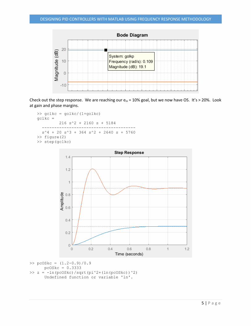
Notice that the log mag plot starts off at 19.1 dB. This is shown by zooming in and using the data cursor.

5 | P a g e


Check out the step response. We are reaching our ess = 10% goal, but we now have OS. It’s > 20%. Look at gain and phase margins.

>> gclkc = golkc/(1+golkc)

gclkc =

216 s^2 + 2160 s + 5184

--------------------------------------

s^4 + 20 s^3 + 364 s^2 + 2640 s + 5760

>> figure(2)

>> step(gclkc)

>> pcOSkc = (1.2-0.9)/0.9

pcOSkc = 0.3333

>> z = -ln(pcOSkc)/sqrt(pi^2+(ln(pcOSkc))^2)

Undefined function or variable 'ln'.

6 | P a g e


Note that Matlab’s function for ln() is log(). Matlab’s function for log() is log10().

>> z = -log(pcOSkc)/sqrt(pi^2+(log(pcOSkc))^2)

z =

0.3301

>> figure(3)

>> margin(golkc)

M = 39.7° , so = 0.397. If we use our formula for %OS as f():

>> z = 0.397

z =

0.3970

>> -log(z)/sqrt(pi^2+(log(z))^2)

ans =

0.2821

%OS = 28.2%. The /M relationship is only an approximation.

Let’s say we want to eliminate ess instead of just reducing it. Thus we shall add a PI controller, i.e. a controller with a pole at the origin (integrator) , a zero (a first-order lead), and a gain. Let’s add the element over which we have no control first—the integrator—and look at its effect. Correct this on the original system, GOL .

>> golint = gol/s

golint =

10

-------------------

s^3 + 10 s^2 + 24 s

>> figure(4)

7 | P a g e


>> bode(golint)

>> grid on

From the figure we can see that with just the integrator, the system is still stable. The gain-crossover frequency is around 0.4 rad/sec, where the phase margin is about 80°, and the phase-crossover frequency is about 5 rad/sec, where the gain margin is 35 dB or so. Let’s see how the system responds to a step input and then decide what to do to add the zero and the gain.

>> gclint = golint/(1+golint)

gclint =

10 s^3 + 100 s^2 + 240 s

--------------------------------------------------

s^6 + 20 s^5 + 148 s^4 + 490 s^3 + 676 s^2 + 240 s

>> figure(2)

>> hold on

>> step(gclint)

8 | P a g e


The steady-state error is indeed gone. But this has been at an extreme cost in system response time.

Perhaps we can use the zero to increase the system speed. Note that the gain-crossover frequency, which

was 10.3 rad/sec or so with the KC adjustment, is now 0.4 rad/sec, more than a 10-fold reduction in speed.

Refer to the Bode plot for golint. On the Bode diagram for the KC-adjusted system, we saw that the gain-

crossover frequency was 13.8 rad/sec. On the Bode plot for golint, at 13.8 rad/sec, the phase angle is

about 40° below 180°. We can try to perform a phase lift here and then adjust the gain to fine-tune our

system. For the full phase lift at 13.8 rad/sec, add the zero one decade before that, i.e. at 1.38 rad/sec.

>> figure(4)

>> bode(golint)

>> grid on

>> hold on

>> golintlead = golint * (1/((1/1.38)*s+1))

>> bode(golintlead)

9 | P a g e


At 10 rad/sec, = -135°, and the log mag value is -24.6 dB. Thus we did indeed lift the phase curve up

above -180° in this frequency range. A phase margin of 45° isn’t bad. Let’s try for this and see what the

outcome is. Apply a gain of 24.6 dB.

>> KC = 10^(24.6/20)

KC =

16.9824

>> golintleadkc = golintlead*KC

golintleadkc =

123.1 s + 169.8

-------------------

s^3 + 10 s^2 + 24 s

>> bode(golintleadkc)

10 | P a g e


This does seem to have had the desired result. Let’s now see the step response, whether the system is

operating quicker without too much %OS.

>> gclintleadkc = golintleadkc/(1+golintleadkc)

gclintleadkc =

123.1 s^4 + 1400 s^3 + 4652 s^2 + 4076 s

-------------------------------------------------------

s^6 + 20 s^5 + 271.1 s^4 + 1880 s^3 + 5228 s^2 + 4076 s

>> figure(2)

>> step(gclintleadkc)

11 | P a g e


Wow! Perfect response: almost as fast as the gain-adjusted system and no steady-state error. Another

phase-lift successfully completed!

It might be possible to further improve the response by adding a second zero somewhere. For example,

additional phase-lift would increase the phase margin and lower the overshoot. Or another zero might

be used to lift the log mag curve and increase the gain-crossover frequency and, thus, the system’s

speed. That would make this then a PID controller. What we have now is a PI controller. Left to do are

to figure out the system’s KP , KI , and KD .

12 | P a g e


Example 2

Now let’s look at a third-order, unity-feedback system subjected to a ramp input. Let

𝐺𝑂𝐿 =10

𝑠 ∙ (𝑠 + 3) ∙ (𝑠 + 9)

>> s = tf('s')

s =

s

>> gol = 10/(s*(s+3)*(s+9))

gol =

10

-------------------

s^3 + 12 s^2 + 27 s

Let’s evaluate this system’s performance by looking at its Bode plot. This will tell us also how we might improve the performance with a PID-family controller.

>> bode(gol)

>> grid on

>> hold on

13 | P a g e


Or close up:

That this is a type 1 system is evidenced by the fact that 1) the log mag curve has an initial slope of -20 dB/dcd and 2) the phase curve starts out at -90°. We are interested in steady-state error and operating this system with a unit ramp input. With the current system, the gain-crossover frequency is about 0.38 rad/sec. For a unit ramp input,

𝑒𝑠𝑠 =1

𝐾𝑣

and Kv = M (the gain-crossover frequency). So

𝑒𝑠𝑠 =1

𝐾𝑣=

1

0.38 rad/sec= 2.63 sec

Let’s verify this. We need to put in a unit ramp input. Matlab doesn’t have a ramp() function. But a unit

step has the Laplace transform 1

𝑠 , and a unit ramp has the Laplace transform

1

𝑠2 . So if we input a unit

step into an integrator, we shall get a unit ramp. Let’s try this.

>> figure(2)

>> step(1/s)

>> grid on

14 | P a g e


This yields the desired result. We can now just multiply our transfer functions by 1/s, subject them to a step, and it’s the same as subjecting them to a unit ramp.

>> hold on

>> gcl = gol/(1+gol)

gcl =

10 s^3 + 120 s^2 + 270 s

--------------------------------------------------

s^6 + 24 s^5 + 198 s^4 + 658 s^3 + 849 s^2 + 270 s

>> step(gcl/s)

Everywhere, the red

line is 2.63 below the

blue line

15 | P a g e


If we look closely, we shall see that the output trails the input by a steady amount, namely 2.63. This is the vertical distance between the desired value (blue) and the actual value (red). As an initial aim, let’s try to halve this ess. For this we can perform a simple gain adjustment. We need to double Kv . For this we need to raise the log mag curve of the open-loop system so that the gain-crossover frequency is at 2*0.38 rad/sec = 0.76 rad/sec. Looking at a close up of the Bode log mag curve, we see that with G( the log mag of the system is at about -6.5 dB at around 0.76 rad/sec.

>> KC = 10^(6.5/20)

KC =

2.1135

Thus if we adjust the log mag curve up by KC = 2.11, we should meet our goal. Let’s do this.

This looks good, now look at the ramp response.

>> figure(2)

>> step(gcl/s)

>> grid on

>> step(1/s)

>> grid on

>> hold on

>> step(gcl/s)

>> step(gclkc/s)

16 | P a g e


The yellow curve does indeed seem to be halfway between the desired value (blue) and the actual value of the original unit ramp response of the original system.

If we want to eliminate ess instead, we need a type two system. Go back to the original system without the gain adjustment and add an integrator.

>> golint = gol/s

golint =

10

---------------------

s^4 + 12 s^3 + 27 s^2

>> figure(4)

>> bode(golint)

>> grid on

>> hold on

17 | P a g e


As the Bode plot shows, adding the pole at the origin has destabilized the system. The phase plot starts out at -180°. This can be easily verified:

figure(5)

>> gclint = golint/(1+golint)

gclint =

10 s^4 + 120 s^3 + 270 s^2

--------------------------------------------------------------

s^8 + 24 s^7 + 198 s^6 + 648 s^5 + 739 s^4 + 120 s^3 + 270 s^2

>> step(1/s)

>> grid on

>> hold on

>> step(gclint/s)

From bode() command From margin() command

18 | P a g e


Yes, it’s indeed unstable. What we might try to do is to perform a phase-lift and raise the phase curve up above -180°. But where? With just the integrator, the gain-crossover frequency is 0.602 rad/sec. Let’s try to raise the curve there. As almost always when adding a lead, we put its break frequency one decade before where we want the lift, because the phase contribution of the lead only reaches the full 90° one decade after the break frequency. Thus let the break frequency be 0.0602 rad/sec. The lead to install is then

𝐺𝑙𝑒𝑎𝑑 = (1

0.0602∙ 𝑠 + 1)

>> golintlead = golint*(1/0.0602*s+1)

golintlead =

166.1 s + 10

---------------------

s^4 + 12 s^3 + 27 s^2

>> figure(4)

>> hold on

>> bode(golintlead)

This did stabilize the system. The gain-crossover frequency is at about 3.4 rad/sec, and there the phase angle is about, well, let’s use the margin command to find out.

>> figure(5)

>> margin(golintlead)

>> grid on

19 | P a g e


The log mag curve crosses 0 dB at 3.63 rad/sec.

As often happens with phase-lifting, the maximum phase contribution is often not exactly where you desire it. The maximum phase occurs at halfway between 0.01 and 1 rad/sec (about 0.03 rad/sec), not at 0.602 rad/sec as we had intended. We could now modify the lead and place its break frequency a bit to the right of 0.0602 rad/sec. But let’s try the simple strategy of de-tuning the log mag curve (multiplying by a gain < 1, which would be negative dB) to make the gain-crossover frequency occur at the maximum phase value. A zoomed-in look at the Bode plot shows

20 | P a g e


This shows that at maximum phase, the log mag curve is at about 24 dB. So lower the log mag curve -24 dB to make this frequency the gain-crossover frequency.

>> KC = 10^(-24/20)

KC =

0.0631

>> golintleadkc = golintlead*KC

golintleadkc =

10.48 s + 0.631

---------------------

s^4 + 12 s^3 + 27 s^2

>> figure(4)

>> bode(golintleadkc)

This seems to have done what we wanted, placed the gain-crossover frequency at the point of

maximum phase-lift. Let’s see how our PI-equipped system (pole at origin/zero somewhere/gain)

responds to a unit ramp input.

>> gclintleadkc

gclintleadkc =

10.48 s^5 + 126.4 s^4 + 290.6 s^3 + 17.04 s^2

--------------------------------------------------------------

s^8 + 24 s^7 + 198 s^6 + 658.5 s^5 + 855.4 s^4 + 290.6 s^3

+ 17.04 s^2

>> step(gclintleadkc/s)

21 | P a g e


Another successful phase-lift. The system has no ess to a ramp input. It does not seem to oscillate

inordinately either. Our controller is

𝐺𝑃𝐼 =0.0631 ∙ (

10.0602

∙ 𝑠 + 1)

𝑠=

𝐾𝑃 ∙ 𝑠 + 𝐾𝐼

𝑠=

𝐾𝐼 ∙ (𝐾𝑃𝐾𝐼

∙ 𝑠 + 1)

𝑠

So KI = 0.0631, KP = 1.05 .

This controller seems to bring the actual value to the desired ramp in 35-40 seconds. We could perhaps

speed the system up by relocating the zero and being less aggressive with trying to suppress the

oscillations (i.e., maybe we have too much phase margin).

Designing PID controllers with Matlab using frequency ...fowen/me422/PIDWithBodeAndMatlab.pdf · 2...

Documents

Transcript of Designing PID controllers with Matlab using frequency ...fowen/me422/PIDWithBodeAndMatlab.pdf · 2...