Designing Embedded Multiprocessor Networks-on-Chip - CiteSeerX

DESIGNING EMBEDDED MULTIPROCESSOR NETWORKS-ON-CHIP

WITH USERS IN MIND

A Thesis

Submitted to the Faculty

of

Carnegie Mellon University

by

Chen-Ling Chou

In Partial Fulfillment of the Requirements for

the Degree of

Doctor of Philosophy

April 2010

ii

© Copyright by Chen-Ling Chou 2010

All Rights Reserved

iii

To my parents Chien-Te Chou, Hui-Yueh Chiang and my husband Hung-Chih Lai

iv

ACKNOWLEDGMENTS

I would like to express my sincere gratitude to all those who have inspired me during my

doctoral study and have supported me in finishing this dissertation.

I especially want to thank my advisor, Professor Radu Marculescu, for his continuous sup-

port, motivation and invaluable guidance during my research and study at Carnegie Mellon

University (CMU). His perpetual energy and enthusiasm in research had motivated all his

advisees, including me. Without his inspiration, patience, friendship and our stimulating dis-

cussions, this dissertation would have never been possible.

I am also grateful to my thesis committee members Professor Shawn Blanton, Dr. Michael

Kishinevsky, Prof. Twan Basten, and Prof. Onur Mutlu for their insightful suggestions and

comments on my research. In particular, I would like to thank Dr. Michael Kishinevsky for

hiring me as an intern at Intel Strategic CAD Lab. The associated experience broadened my

perspective on the practical aspects in the industry.

All my lab buddies at the Center for Silicon System Implementation (CSSI) of CMU made

it a convivial place to work. In particular, I would like to thank my colleagues at our System

Level Design (SLD) group, i.e. Paul Bogdan, Shun-ping Chiu, Cory Bevilacqua, Miray Kas,

and all previous members of SLD group, i.e. Jung-Chun (Mike) Kao, Umit Ogras, Nicholas H.

Zamora, and Ting-Chun Huang; They had inspired me in research and life through our interac-

tions during the long hours in the lab. Thanks.

v

I would also like to thank all of my friends in Pittsburgh who made this city a better place

to live. In particular, I would like to thank my badminton friends in CMU and University of

Pittsburgh, who have made my Ph.D. life more fruitful and exciting. Playing badminton regu-

larly with them makes me full of energy, as well as contributes to my persistence and hard-

working in research.

My deepest gratitude goes to my family (my mom Hui-Yueh Chiang, my father Chien-Te

Chou, and my husband Hung-Chih Lai) for their unflagging love and support throughout my

life; this dissertation is simply impossible without them. In particular, without the encourage-

ment and support from Hung-Chih, my graduate study would have finished much earlier with-

out a Ph.D. degree.

Finally, I would like to express my gratitude to several funding agencies, National Science

Foundation and Gigascale Systems Research Center, one of five research centers funded under

the Focus Center Research Program, a Semiconductor Research Corporation program.

vi

TABLE OF CONTENTS

Page

LIST OF TABLES . . . . . . . . . . . . . . . . . . . . . . . . . . . . . . . . . . . . . . . . . . . . . . . . . . . . . . . xi

LAST OF FIGURES . . . . . . . . . . . . . . . . . . . . . . . . . . . . . . . . . . . . . . . . . . . . . . . . . . . . . . xiii

ABBREVIATIONS. . . . . . . . . . . . . . . . . . . . . . . . . . . . . . . . . . . . . . . . . . . . . . . . . . . . . . . xviii

ABSTRACT . . . . . . . . . . . . . . . . . . . . . . . . . . . . . . . . . . . . . . . . . . . . . . . . . . . . . . . . . . . . xx

1. Introduction . . . . . . . . . . . . . . . . . . . . . . . . . . . . . . . . . . . . . . . . . . . . . . . . . . . . . . . . . . . 1

1.1. Trends and Challenges for Embedded Systems . . . . . . . . . . . . . . . . . . . . . . . .1

1.2. Evolution of Embedded System Design . . . . . . . . . . . . . . . . . . . . . . . . . . . . . .3

1.3. Motivation for User-Centric Design. . . . . . . . . . . . . . . . . . . . . . . . . . . . . . . . .8

1.3.1. User Behavior Variation . . . . . . . . . . . . . . . . . . . . . . . . . . . . . . . . . . . . .8

1.3.2. Proposed User-aware Design Methodology . . . . . . . . . . . . . . . . . . . . . .12

1.4. Dissertation Overview . . . . . . . . . . . . . . . . . . . . . . . . . . . . . . . . . . . . . . . . . . .15

1.4.1. DSE for Full-custom NoC with Predictable System Configurations . . .15

1.4.2. User-centric Design Methodology Handling Unpredictable System

Configurations . . . . . . . . . . . . . . . . . . . . . . . . . . . . . . . . . . . . . . . . . . . .15

1.5. Dissertation Organization . . . . . . . . . . . . . . . . . . . . . . . . . . . . . . . . . . . . . . . . .20

2. Embedded NoC Platform Characterization. . . . . . . . . . . . . . . . . . . . . . . . . . . . . . . . . . . 23

2.1. NoC Architecture . . . . . . . . . . . . . . . . . . . . . . . . . . . . . . . . . . . . . . . . . . . . . . .23

2.2. Application Modeling. . . . . . . . . . . . . . . . . . . . . . . . . . . . . . . . . . . . . . . . . . . .29

2.3. Trace-based Energy Modeling . . . . . . . . . . . . . . . . . . . . . . . . . . . . . . . . . . . . .30

2.3.1. User Trace Modeling . . . . . . . . . . . . . . . . . . . . . . . . . . . . . . . . . . . . . . .31

2.3.2. Computation Energy Modeling . . . . . . . . . . . . . . . . . . . . . . . . . . . . . . .32

vii

2.3.3. Communication Energy Modeling . . . . . . . . . . . . . . . . . . . . . . . . . . . . .33

3. System Interconnect DSE for Full-custom NoC Platforms . . . . . . . . . . . . . . . . . . . . . . 35

3.1. Introduction. . . . . . . . . . . . . . . . . . . . . . . . . . . . . . . . . . . . . . . . . . . . . . . . . . . .35

3.2. Previous Work . . . . . . . . . . . . . . . . . . . . . . . . . . . . . . . . . . . . . . . . . . . . . . . . .37

3.3. System Interconnect in MPSoC . . . . . . . . . . . . . . . . . . . . . . . . . . . . . . . . . . . .38

3.3.1. General Framework for Application-specific MPSoC . . . . . . . . . . . . . .38

3.3.2. System Interconnect Problem Formulation . . . . . . . . . . . . . . . . . . . . . .40

3.3.3. Communication Fabric Exploration Flow . . . . . . . . . . . . . . . . . . . . . . .43

3.4. Optimization of System Interconnect Problem. . . . . . . . . . . . . . . . . . . . . . . . .45

3.4.1. Exact System Interconnect Exploration . . . . . . . . . . . . . . . . . . . . . . . . .45

3.4.2. Heuristic for Speeding up System Interconnect Exploration . . . . . . . . .48

3.5. Experimental Results . . . . . . . . . . . . . . . . . . . . . . . . . . . . . . . . . . . . . . . . . . . .50

3.5.1. Industrial Case Study . . . . . . . . . . . . . . . . . . . . . . . . . . . . . . . . . . . . . . .50

3.5.2. Synthetic Applications for Larger Systems . . . . . . . . . . . . . . . . . . . . . .53

3.6. Summary. . . . . . . . . . . . . . . . . . . . . . . . . . . . . . . . . . . . . . . . . . . . . . . . . . . . . .55

4. User-Centric DSE for Heterogeneous Embedded NoCs. . . . . . . . . . . . . . . . . . . . . . . . . 57

4.1. Introduction. . . . . . . . . . . . . . . . . . . . . . . . . . . . . . . . . . . . . . . . . . . . . . . . . . . .57

4.2. Related Work . . . . . . . . . . . . . . . . . . . . . . . . . . . . . . . . . . . . . . . . . . . . . . . . . .58

4.3. Preliminaries . . . . . . . . . . . . . . . . . . . . . . . . . . . . . . . . . . . . . . . . . . . . . . . . . . .59

4.4. The Problem and Steps for DSE. . . . . . . . . . . . . . . . . . . . . . . . . . . . . . . . . . . .62

4.4.1. User Behavior Similarity and Clustering . . . . . . . . . . . . . . . . . . . . . . . .62

4.4.2. Automated NoC Platform Generation . . . . . . . . . . . . . . . . . . . . . . . . . .65

4.4.3. Validation Process . . . . . . . . . . . . . . . . . . . . . . . . . . . . . . . . . . . . . . . . .70


4.5.1. Evaluation of User Behavior Clustering. . . . . . . . . . . . . . . . . . . . . . . . .73

Page

viii

4.5.2. NoC Platform Evaluation . . . . . . . . . . . . . . . . . . . . . . . . . . . . . . . . . . . .75

4.5.3. Evaluation of Entire Design Methodology . . . . . . . . . . . . . . . . . . . . . . .76

4.6. Summary. . . . . . . . . . . . . . . . . . . . . . . . . . . . . . . . . . . . . . . . . . . . . . . . . . . . . .77

5. Energy- and Performance-Aware Incremental Mapping for NoC . . . . . . . . . . . . . . . . . 79

5.1. Introduction. . . . . . . . . . . . . . . . . . . . . . . . . . . . . . . . . . . . . . . . . . . . . . . . . . . .79

5.2. Related Work . . . . . . . . . . . . . . . . . . . . . . . . . . . . . . . . . . . . . . . . . . . . . . . . . .83

5.3. Motivational Example . . . . . . . . . . . . . . . . . . . . . . . . . . . . . . . . . . . . . . . . . . .84

5.4. Incremental Run-time Mapping Problem . . . . . . . . . . . . . . . . . . . . . . . . . . . . .86

5.4.1. Proposed Methodology. . . . . . . . . . . . . . . . . . . . . . . . . . . . . . . . . . . . . .86

5.4.2. Problem Formulation . . . . . . . . . . . . . . . . . . . . . . . . . . . . . . . . . . . . . . .88

5.4.3. Significance of the Problem . . . . . . . . . . . . . . . . . . . . . . . . . . . . . . . . . .89

5.5. Solving the Incremental Mapping Problem . . . . . . . . . . . . . . . . . . . . . . . . . . .90

5.5.1. Solutions to the Near Convex Region Selection Problem. . . . . . . . . . . .90

5.5.2. Solutions to the Vertex Allocation Problem . . . . . . . . . . . . . . . . . . . . . .103


5.6.1. Evaluation of Region Selection Algorithm on Random Applications. . .107

5.6.2. Evaluation of Vertex Allocation Algorithm on Random Applications . .109

5.6.3. Random Applications Considering Energy Overhead for the Entire Incremental Mapping Process. . . . . . . . . . . . . . . . . . . . . . . . . . . . . . . . .111

5.6.4. Real Applications Considering Energy Overhead for the Entire Incremental Mapping Process . . . . . . . . . . . . . . . . . . . . . . . . . . . . . . . . .112

5.7. Summary. . . . . . . . . . . . . . . . . . . . . . . . . . . . . . . . . . . . . . . . . . . . . . . . . . . . . .114

6. Fault-tolerant Techniques for On-line Resource Management . . . . . . . . . . . . . . . . . . . . 117

6.1. Introduction. . . . . . . . . . . . . . . . . . . . . . . . . . . . . . . . . . . . . . . . . . . . . . . . . . . .117

6.2. Related Work and Novel Contributions . . . . . . . . . . . . . . . . . . . . . . . . . . . . . .120

6.3. Analysis for Network Contention and Spare Core Placement . . . . . . . . . . . . .121

Page

ix

6.3.1. Network Contention Impact . . . . . . . . . . . . . . . . . . . . . . . . . . . . . . . . . .121

6.3.2. Spare Core Placement . . . . . . . . . . . . . . . . . . . . . . . . . . . . . . . . . . . . . . .125

6.4. Investigations Involving New Metrics . . . . . . . . . . . . . . . . . . . . . . . . . . . . . . .129

6.5. Fault-tolerant Resource Management. . . . . . . . . . . . . . . . . . . . . . . . . . . . . . . .133

6.5.1. RUN_FT_MAPPING Process . . . . . . . . . . . . . . . . . . . . . . . . . . . . . . . . . . .134

6.5.2. RUN_FT_MAPPING Algorithm . . . . . . . . . . . . . . . . . . . . . . . . . . . . . . . . .135


6.6.1. Evaluation with Specific Patterns . . . . . . . . . . . . . . . . . . . . . . . . . . . . . .138

6.6.2. Impact of Failure Rates with Spare Core Placement . . . . . . . . . . . . . . . .140

6.6.3. Evaluation with Real Applications . . . . . . . . . . . . . . . . . . . . . . . . . . . . .141

6.7. Summary. . . . . . . . . . . . . . . . . . . . . . . . . . . . . . . . . . . . . . . . . . . . . . . . . . . . . .142

7. User-Aware Dynamic Task Allocation . . . . . . . . . . . . . . . . . . . . . . . . . . . . . . . . . . . . . . 143

7.1. Introduction. . . . . . . . . . . . . . . . . . . . . . . . . . . . . . . . . . . . . . . . . . . . . . . . . . . .143

7.2. Related Work . . . . . . . . . . . . . . . . . . . . . . . . . . . . . . . . . . . . . . . . . . . . . . . . . .147

7.3. Preliminaries and Methodology Overview. . . . . . . . . . . . . . . . . . . . . . . . . . . .148

7.3.1. Motivational Examples . . . . . . . . . . . . . . . . . . . . . . . . . . . . . . . . . . . . . .148

7.3.2. System Description . . . . . . . . . . . . . . . . . . . . . . . . . . . . . . . . . . . . . . . . .153

7.3.3. Overview of the proposed methodology . . . . . . . . . . . . . . . . . . . . . . . . .155

7.3.4. User Modeling . . . . . . . . . . . . . . . . . . . . . . . . . . . . . . . . . . . . . . . . . . . . .157

7.4. Problem Formulation of User-Aware Task Allocation Process . . . . . . . . . . .159

7.5. User-Aware Task Allocation Approaches . . . . . . . . . . . . . . . . . . . . . . . . . . . .162

7.5.1. Solving the Region Forming Sub-problem (P1) . . . . . . . . . . . . . . . . . . .162

7.5.2. Solving the Region Rotation Sub-problem (P2) . . . . . . . . . . . . . . . . . . .165

7.5.3. Solving the Region Selection Sub-problem (P3). . . . . . . . . . . . . . . . . . .168

7.5.4. Solving the Application Mapping Sub-problem (P4) . . . . . . . . . . . . . . .168

Page

x

7.6. Light-Weight Model Learning Process . . . . . . . . . . . . . . . . . . . . . . . . . . . . . .168


7.7.1. Evaluation on Random Applications . . . . . . . . . . . . . . . . . . . . . . . . . . . .173

7.7.2. Real Applications with Run-time Energy Overhead Considered . . . . . .177

7.7.3. Real Applications with On-line Learning of User Model . . . . . . . . . . . .180

7.8. Summary. . . . . . . . . . . . . . . . . . . . . . . . . . . . . . . . . . . . . . . . . . . . . . . . . . . . . .183

8. Conclusions and Future Directions . . . . . . . . . . . . . . . . . . . . . . . . . . . . . . . . . . . . . . . . . 185

8.1. Dissertation Contributions . . . . . . . . . . . . . . . . . . . . . . . . . . . . . . . . . . . . . . . .185

8.2. Future Directions . . . . . . . . . . . . . . . . . . . . . . . . . . . . . . . . . . . . . . . . . . . . . . .188

8.2.1. Challenges Ahead for User-centric Embedded System Design . . . . . . .188

8.2.2. Increasing Flow Experience by Designing Embedded Systems . . . . . . .189

LIST OF REFERENCES . . . . . . . . . . . . . . . . . . . . . . . . . . . . . . . . . . . . . . . . . . . . . . . . . . 193

APPENDIX A. Machine Learning Techniques Survey for User-centric Design . . . . . . . . 203

APPENDIX B. ILP-based Contention-aware Application Mapping . . . . . . . . . . . . . . . . . 207

B.1. Introduction . . . . . . . . . . . . . . . . . . . . . . . . . . . . . . . . . . . . . . . . . . . .207

B.2. Preliminaries . . . . . . . . . . . . . . . . . . . . . . . . . . . . . . . . . . . . . . . . . . .207

B.3. Problem Formulation . . . . . . . . . . . . . . . . . . . . . . . . . . . . . . . . . . . . .209

B.4. ILP-based Contention-aware Mapping Approach . . . . . . . . . . . . . . .210

B.4.1. Parameters and Variables . . . . . . . . . . . . . . . . . . . . . . . . . .210

B.4.2. Objective Function . . . . . . . . . . . . . . . . . . . . . . . . . . . . . . .211

B.4.3. Constraints . . . . . . . . . . . . . . . . . . . . . . . . . . . . . . . . . . . . .212

B.5. Experimental Results . . . . . . . . . . . . . . . . . . . . . . . . . . . . . . . . . . . . .213

B.5.1. Experiments using Synthetic Applications . . . . . . . . . . . . .213

B.5.2. Experiments using Real Applications . . . . . . . . . . . . . . . . .215

B.6. Summary . . . . . . . . . . . . . . . . . . . . . . . . . . . . . . . . . . . . . . . . . . . . . .217

Page

xi

LIST OF TABLES

Table Page

1.1 Three different categories of user-system interaction. . . . . . . . . . . . . . . . . . . . . . . . 11

2.1 Impact of adding the control network on area. The synthesis is performed for Xilinx Virtex-II Pro XC2VP30 FPGA.. . . . . . . . . . . . . . . . . . . . . . . . . . . . . . . . . . . . . . . . 28

4.1 Architecture template for the NoC platform. . . . . . . . . . . . . . . . . . . . . . . . . . . . . . . 72

4.2 Computation energy consumption comparison for three trace clusters and different resource sets derived by the proposed and traditional design flow. . . . . . . . . . . . . . 75

5.1 L1(R’) + L1(R-R’) minimization problem when using the Euclidean Minimum (EM), Fixed Center (FC), and Neighbor_aware Frontier (NF) heuristics. . . . . . . . . 97

5.2 Mapping approach proposed in [27] vs. our algorithms results. . . . . . . . . . . . . . 114

6.1 Comparison among the Random, MBS [99], and Nearest Neighbor (NN) [27] mapping methods.. . . . . . . . . . . . . . . . . . . . . . . . . . . . . . . . . . . . . . . . . . . . . . . . . . . . . . 132

6.2 Throughput and Energy Consumption between proposed FT and Nearest Neighbor (NN) approaches for all-to-all and one-to-all communication patterns. . . . . . . . . 139

6.3 Impact of contamination area on different failure rates under Side and Random spare core placements. . . . . . . . . . . . . . . . . . . . . . . . . . . . . . . . . . . . . . . . . . . . . . . . 140

6.4 Comparison between the Nearest Neighbor (NN) and our FT mapping results on the overall system performance. . . . . . . . . . . . . . . . . . . . . . . . . . . . . . . . . . . . . . . . 142

7.1 Event communication cost [in bits] for three approaches and five applications entering in the system as shown in Figure 7.2. . . . . . . . . . . . . . . . . . . . . . . . . . . . . 151

7.2 Comparison of communication consumption among different approaches on a different size NoCs. . . . . . . . . . . . . . . . . . . . . . . . . . . . . . . . . . . . . . . . . . . . . . . . . . 177

7.3 Comparison of the run-time overhead and the overall communication energy savings under four implementations on a 5 × 5 mesh NoC. . . . . . . . . . . . . . . . . . . 180

xii

7.4 Normalized event cost in stages 1, 2, and 3 under different user models from four users normalized to the total event cost of “Nearest Neighbor [27]” approach.. . . . 181

B.1 Energy and throughput comparison between energy-aware in [79] and contention-aware mapping. . . . . . . . . . . . . . . . . . . . . . . . . . . . . . . . . . . . . . . . . . . . . . . . . . . . . 214

B.2 Communication energy overhead and throughput improvement of our contention- aware solution compared to the energy-aware solution [79]. . . . . . . . . . . . . . . . . . 215

PageTable

xiii

LIST OF FIGURES

Figure Page

1.1 General idea of newly proposed user-centric design. . . . . . . . . . . . . . . . . . . . . . . . 3

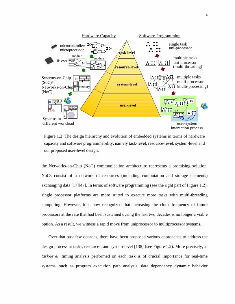
1.2 The design hierarchy and evolution of embedded systems in terms of hardware capacity and software programmability, namely task-level, resource-level, system- level and our proposed user-level design. . . . . . . . . . . . . . . . . . . . . . . . . . . . . . . . . 4

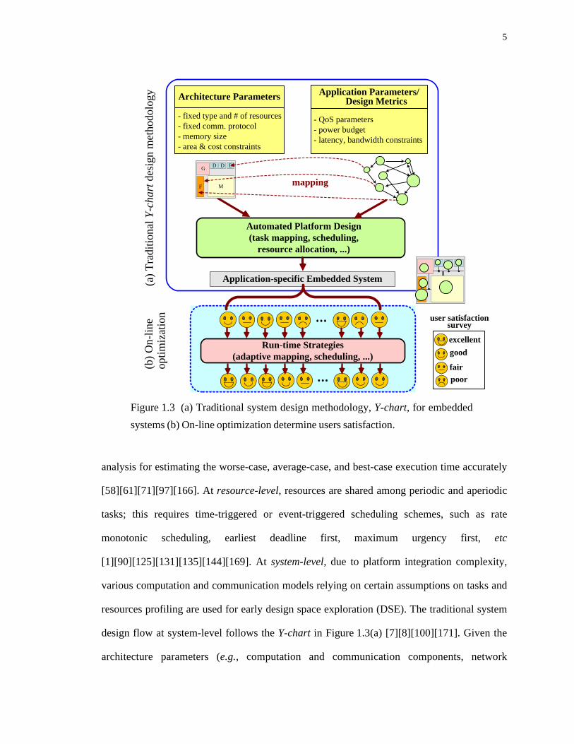
1.3 (a) Traditional system design methodology, Y-chart, for embedded systems (b) On- line optimization determine users satisfaction. . . . . . . . . . . . . . . . . . . . . . . . . . . . . 5

1.4 Hierarchy of needs at each level of abstraction from system designer and user perspectives. . . . . . . . . . . . . . . . . . . . . . . . . . . . . . . . . . . . . . . . . . . . . . . . . . . . . . . . . . 7

1.5 Three-day user traces from two users. (a) Appearances of five different Windows applications (b) Total number of applications in the system of each time instant. . 9

1.6 User satisfaction ratings corresponding to different CPU usage for two users. . . . 10

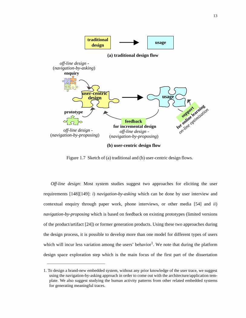
1.7 Sketch of (a) traditional and (b) user-centric design flows. . . . . . . . . . . . . . . . . . . 13

1.8 User-centric design flow for heterogeneous NoCs, including user behavior analysis, NoC architecture automation, and optimization process. Five types of problems with the “*” sign with their related machine learning techniques are surveyed in Appendix A.. . . . . . . . . . . . . . . . . . . . . . . . . . . . . . . . . . . . . . . . . . . . . . . . . . . . . . . 17

2.1 Homogeneous or heterogeneous 2-D mesh NoCs with PEs and interconnect via the data and control networks described in a generalized way.. . . . . . . . . . . . . . . . . . . 25

2.2 (a) The logical view of the control network. (b) The on-chip router micro-architecture that handles the control network.. . . . . . . . . . . . . . . . . . . . . . . . . . . . . . . . . 27

2.3 Application Characterization Graph (ACG) characteristics. The tasks belonging to the same vertex are mapped onto the same PE. Each edge represents the communication between two nodes. . . . . . . . . . . . . . . . . . . . . . . . . . . . . . . . . . . . . . . . . . . 29

3.1 Block diagram for a general MPSoC platform. . . . . . . . . . . . . . . . . . . . . . . . . . . . 38

3.2 General platform with multiple IPs communicated via the system interconnect. . . 39

xiv

3.3 (a) System interconnect design space trading off the system performance and area/ wirelength overhead (b) Traditional bus model connecting four IP blocks (c) Fully connected switches with four IP blocks (d) Possible optimized communication fabric for four IP blocks. . . . . . . . . . . . . . . . . . . . . . . . . . . . . . . . . . . . . . . . . . . . . . 42

3.4 The flow of the communication fabric design space exploration with the analysis, simulation, and evaluation stages shown explicitly. . . . . . . . . . . . . . . . . . . . . . . . . 44

3.5 A three-IP example of communication fabric exploration using the branch and bound algorithm. . . . . . . . . . . . . . . . . . . . . . . . . . . . . . . . . . . . . . . . . . . . . . . . . . . . 46

3.6 The pseudo code of the system interconnect exploration using the branch and bound method. . . . . . . . . . . . . . . . . . . . . . . . . . . . . . . . . . . . . . . . . . . . . . . . . . . . . . 47

3.7 The proposed heuristic for four IPs with the number of muxes set to 2. . . . . . . . . 49

3.8 System interconnect exploration for a real SoC design. (a) Pareto-optimal set (latency vs. fabric area) obtained via analysis. (b) Simulation results for solutions in (a). (c) Pareto-optimal set (i.e., latency vs. fabric wirelength) obtained via analysis. (d) Simulation results for solutions in (c). . . . . . . . . . . . . . . . . . . . . . . . . 51

3.9 Forty non-Pareto points and Pareto curve plots obtained via analysis (a) and via simulation (b). . . . . . . . . . . . . . . . . . . . . . . . . . . . . . . . . . . . . . . . . . . . . . . . . . . . . . 52

3.10 Solutions comparison between branch and bound method (BB) and the proposed heuristic for system interconnect exploration of a synthetic application with 13 IP blocks. . . . . . . . . . . . . . . . . . . . . . . . . . . . . . . . . . . . . . . . . . . . . . . . . . . . . . . . . . . . 54

3.11 Run-time and solution quality comparison between branch and bound approach (BB) and our heuristic as the system size scales up. . . . . . . . . . . . . . . . . . . . . . . . . 54

4.1 The proposed user-centric design flow in terms of the off-line DSE processes. . . 60

4.2 Main steps of user behavior clustering. . . . . . . . . . . . . . . . . . . . . . . . . . . . . . . . . . 64

4.3 Main steps for computational resource selection.. . . . . . . . . . . . . . . . . . . . . . . . . . 66

4.4 Main steps for resource location assignment. . . . . . . . . . . . . . . . . . . . . . . . . . . . . . 69

4.5 Validation process of the newly proposed methodology.. . . . . . . . . . . . . . . . . . . . 71

4.6 Pareto points showing the tradeoffs between price and computation energy consumption. For each cluster, four users are randomly selected and their Pareto curves are plotted. . . . . . . . . . . . . . . . . . . . . . . . . . . . . . . . . . . . . . . . . . . . . . . . . . . 74

5.1 Example of NoC incremental application mapping comparing the greedy and our proposed solutions. The greedy approach which does not consider additional mappings incurs higher communication overhead for App 2, and the system

PageFigure

xv

communication cost as well, compared to our proposed solution. . . . . . . . . . . . . . 80

5.2 Motivational example for incremental mapping process. (a) Optimal solution (b) Near convex region solution. . . . . . . . . . . . . . . . . . . . . . . . . . . . . . . . . . . . . . . . . . . . . . . 85

5.3 Overview of the proposed incremental mapping methodology.. . . . . . . . . . . . . . . 86

5.4 Overview of the proposed methodology. (a) The incoming application ACG (b) Current system configuration (c) The near convex region selection step (d) The ver-tex allocation step. . . . . . . . . . . . . . . . . . . . . . . . . . . . . . . . . . . . . . . . . . . . . . . . . . . 87

5.5 The impact of Manhattan Distance (MD) on communication energy consumption for four different scenarios (S1-S4). . . . . . . . . . . . . . . . . . . . . . . . . . . . . . . . . . . . 90

5.6 L1(R’) + L1(R-R’) minimization problem: select a region R’, such that the sum of the total Manhattan Distance (MD) between any pair of tiles inside region R and that inside region R-R’ is minimized. . . . . . . . . . . . . . . . . . . . . . . . . . . . . . . . 91

5.7 Region with N = 20 resulting from several distinct methods, namely (a) Best Case (BC) (b) Worst Case (WC) (c) Euclidean Minimum (EM) (d) Fixed Center (FC) (e) Random Frontier (RF) (f) Neighbor_aware Frontier (NF). Note that the shape of the resulted regions would be the same even if shifted to other coordinates. Here, we only consider minimizing the total Manhattan Distance between any pair of these N tiles inside R’, i.e., L1(R’). . . . . . . . . . . . . . . . . . . . . . . . . . . . . . . . . . . . . . 92

5.8 L1 distance results showing the scalability of the solutions obtained via the Best Case (BC), Worst Case (WC) and four heuristics (EM, FC, RF, and NF).. . . . . . . 95

5.9 Histogram over 1000 runs for L1(R’) + L1(R-R’) minimization problem. We represent [L1(R’) + L1(R-R’)] distances on the x-axis and their frequency of occurrence on the y-axis. . . . . . . . . . . . . . . . . . . . . . . . . . . . . . . . . . . . . . . . . . . . . . . . . . . . . . . 97

5.10 Dispersion and Centrifugal factor calculation example. . . . . . . . . . . . . . . . . . . . 99

5.11 Near convex region selection algorithm. . . . . . . . . . . . . . . . . . . . . . . . . . . . . . . 100

5.12 Incremental run-time mapping process. (a) The ACG of the incoming application (b) Current system behavior (c) Near convex region selection process (d) Vertex allocation process. . . . . . . . . . . . . . . . . . . . . . . . . . . . . . . . . . . . . . . . . . . . . . . . . . .101

5.13 Vertex allocation algorithm. . . . . . . . . . . . . . . . . . . . . . . . . . . . . . . . . . . . . . . . . 104

5.14 Vertex allocation process based on the example in Figure 5.12. (a) Initial configuration with every vertex white. (b) Vertex 6 is discovered. (c) Vertex 9 is discovered. (d) Vertex 7 is finished and colored black. (e) Vertex 9 is colored from gray to black. (f) Vertex 6 is colored from gray to black (g) Vertex allocation process is done; all vertices are colored black. . . . . . . . . . . . . . . . . . . . . . . . . . . . 105

PageFigure

xvi

5.15 (a) Impact of selection region process on inter-processor communication. (b) Com- munication energy loss: optimal mapping vs. our allocation algorithm given a selected region. (c) Optimal vs. our allocation algorithm under different communication rates. (d) Communication energy savings: arbitrary mapping vs. our allocation algorithm. . . . . . . . . . . . . . . . . . . . . . . . . . . . . . . . . . . . . . . . . . . . . . . . . 108

5.16 Communication energy consumption comparison using random applications. . . 111

6.1 Non-ideal 2-D mesh platform consists of resources connected via a network. The resources include computational tiles (i.e., manager titles, active and spare cores) and memory titles. Permanent, transient, or intermittent faults may affect the computational and communication components on this platform. . . . . . . . . . . . . . 118

6.2 Application mapping on mesh-based 3 × 3 NoC (a) Application characteristic ACG = (V, E) (b) Source-based contention (c) Destination-based contention (d) Path-based contention. . . . . . . . . . . . . . . . . . . . . . . . . . . . . . . . . . . . . . . . . . . . . 122

6.3 The (a) source-based (b) destination-based (c) path-based contention impact on average packet latency. . . . . . . . . . . . . . . . . . . . . . . . . . . . . . . . . . . . . . . . . . . . . . . 123

6.4 (a) Application Characterization Graph (ACG) (b) Spare cores (‘S’) are assigned towards the side of the system. (c) Spare cores ‘S’ are randomly distributed in the system (d) Spare cores ‘S’ are evenly distributed in the system. . . . . . . . . . . . . . . 126

6.5 Quantitative analysis on the performance impact on three different spare core placements. . . . . . . . . . . . . . . . . . . . . . . . . . . . . . . . . . . . . . . . . . . . . . . . . . . . . . . . 128

6.6 Two mapping results for the ACG in Figure 6.4(a) where the spare cores are randomly placed on the platform. . . . . . . . . . . . . . . . . . . . . . . . . . . . . . . . . . . . . . . . . . 131

6.7 3D Kiviat plots showing WMD, LCC, and SFF metrics for three difference mapping schemes (i.e., Random, MBS, and NN). . . . . . . . . . . . . . . . . . . . . . . . . . . . . . . 132

6.8 The FT resource management framework. . . . . . . . . . . . . . . . . . . . . . . . . . . . . . . . 134

6.9 Main steps of RUN_MIGRATION process. . . . . . . . . . . . . . . . . . . . . . . . . . . . . . . . . 135

6.10 Main steps of RUN_FT_MAPPING process. . . . . . . . . . . . . . . . . . . . . . . . . . . . . . . 137

7.1 Contiguous (a) and non-contiguous (b)-(e) allocations for four applications using standard techniques.. . . . . . . . . . . . . . . . . . . . . . . . . . . . . . . . . . . . . . . . . . . . . . . . . 144

7.2 Motivational example of run-time resource management with user behavior taken into consideration. (a) Application characteristics. (b) Events in the system. (c)(d)(e) Task allocation scheme under Approach 1, Approach 2, and Hybrid approach, respectively. . . . . . . . . . . . . . . . . . . . . . . . . . . . . . . . . . . . . . . . . . . . . . . . . 149

7.3 Overview of the proposed methodology. Default approach (i.e., Approach 2) is

PageFigure

xvii

applied in stage 1. Hybrid approach with pre-defined user model is applied in stage 2. Hybrid approach with on-line learned user model is applied in stage 3. . . 155

7.4 Algorithm flow for our proposed methodology.. . . . . . . . . . . . . . . . . . . . . . . . . . . 156

7.5 Main steps of the region forming algorithm. . . . . . . . . . . . . . . . . . . . . . . . . . . . . . 163

7.6 Example showing the region forming algorithm on an ACG. . . . . . . . . . . . . . . . . 164

7.7 The subtraction calculation during the region rotation process. . . . . . . . . . . . . . . . 166

7.8 Main steps of the region rotation algorithm.. . . . . . . . . . . . . . . . . . . . . . . . . . . . . . 167

7.9 Four possible decision tree structures for user model. . . . . . . . . . . . . . . . . . . . . . . 169

7.10 4-fold cross-validation for model learning. . . . . . . . . . . . . . . . . . . . . . . . . . . . . . 171

7.11 (a) Pseudo codes of tree structure learning process without cross-validation method and (b)(c) with cross-validation method. . . . . . . . . . . . . . . . . . . . . . . . . . . 162

7.12 Communication energy loss compared to the optimal solution for (a) region forming (P1) sub-problem and (b) application mapping (P4) sub-problem on a 2D- mesh NoC. . . . . . . . . . . . . . . . . . . . . . . . . . . . . . . . . . . . . . . . . . . . . . . . . . . . . . . . . 174

7.13 (a) Communication cost comparison among Approach 1, Approach 2, and the hybrid approach (which considers the user behavior) on an 8 × 8 NoC. (b) L(R) where R is the available/unused resources comparison among Approach 1, Ap- proach 2, and thee hybrid approach. . . . . . . . . . . . . . . . . . . . . . . . . . . . . . . . . . . . . 176

8.1 Model exploration for user-centric design flow. . . . . . . . . . . . . . . . . . . . . . . . . . . 188

8.2 Four-quadrant states in terms of challenge and skill level.. . . . . . . . . . . . . . . . . . . 191

A.1 (a) Five types of problems for user-centric design i) classification ii) regression iii) similarity iv) clustering v) reinforcement learning (b) Selected machine learning approaches. . . . . . . . . . . . . . . . . . . . . . . . . . . . . . . . . . . . . . . . . . . . . . . . . . . . .204

B.1 (a) Logical and (b) physical application characterization graph. (c) one core mapping example.. . . . . . . . . . . . . . . . . . . . . . . . . . . . . . . . . . . . . . . . . . . . . . . . . . . . . . 208

B.2 Path-based contention count in a 4 × 4 NoC comparing the random, energy-aware in [79] and contention-aware mapping. . . . . . . . . . . . . . . . . . . . . . . . . . . . . . . . . . . 214

B.3 (a) Parallel-1 benchmark (b)(c) Mapping results of the energy-aware approach [79] and our contention-aware method (d) Average packet latency and throughput comparison under these two mapping methods. . . . . . . . . . . . . . . . . . . . . . . . . . . . 216

PageFigure

xviii

ABBREVIATIONS

ACG Application characterization graph

CC Computation capacities

CMP Chip multiprocessors

DSE Design space exploration

DSP Digital signal processor

E3S Embedded system synthesis benchmark

GM Global manager

FCA Failure contamination area

FIFO First-in-first-out

FT Fault tolerant

GPU Graphics processing units

IDC Identification content

ILP Integer linear programming

I/O Input/output

IP Intellectual property

LACG Logical application characterization graph

MCR Minimal computation requirement

MD Manhattan distance

MPSoC Multiprocessor Systems-on-Chip

NI Network interface

NN Nearest neighbor

NoC Networks-on-Chip

OS Operating system

PACG Physical application characterization graph

PCI Peripheral component interconnect

xix

PDA Personal digital assistant

PE Processing element

PL Port location

PTM Predictive technology model

RMS Recognition, mining, and synthesis

SATA Serial advanced technology attachment

SoC Systems-on-Chip

UART Universal asynchronous receiver/transmitter

USB Universal serial bus

WCET Worst case execution time

xx

ABSTRACT

Future embedded Systems-on-Chip (SoCs) designed at nanoscale will likely consist of

tens or hundreds of (potentially energy-efficient) heterogeneous cores supporting one or sev-

eral dedicated applications. For such systems, the Networks-on-Chip (NoC) communication

architectures have been proposed as a scalable solution which consists of a network of

resources exchanging packets while running various applications concurrently. Over recent

years, embedded systems have gained an enormous amount of processing power and function-

ality with the ultimate goal on power and performance optimization.

In this dissertation, with the ultimate goal that any system optimization is to satisfy the end

user, we study outstanding problems on embedded system methodology, while incorporating

the user behavior information into the modeling, analysis, optimization, and evaluation steps.

Our specific contributions are as follows.

• For predictable system configurations derived from use-case applications, we explore

the design space of system interconnect on application-specific multi-processor sys-

tems-on-chips (MPSoCs). With the proposed analytical and simulation models, we can

theoretically generate fabric solutions with optimal cost-performance trade-offs, while

considering various design constrains, such as power, area, and wirelength.

• For unpredictable system configurations incorporating users’ interaction with the sys-

tem, we present a new design methodology for automatically generating regular NoC

platforms, while including explicitly the information about the user experience into the

xxi

design process. Such off-line design flow aims at minimizing the workload variance and

allows the system to better adapt to different types of uses.

• For applications entering and leaving the system dynamically, we propose an efficient

technique for run-time application mapping onto heterogeneous NoC platforms

with the goal of minimizing the communication energy consumption, while still

providing performance guarantees. The proposed technique allows for new appli-

cations to be easily added to the system platform with minimal inter-processor

communication overhead.

• To address the problem of runtime resource management in NoC platforms while con-

sidering permanent, transient, and intermittent failures, we propose a system-level fault-

tolerant approach that investigates several metrics for network contention and system

fragmentation, as well as their impacts on system performance.

• Finally, having generated system platforms which exhibit less variation among the

users’ behavior, we explore flexible and extensible run-time resource management tech-

niques that allow system to adapt to run-time stimuli specific to each class of user

behaviors; these techniques change dynamically according to the user models built on-

line based on different user needs.

1

1. INTRODUCTION

1.1. Trends and Challenges for Embedded Systems

Embedded systems consist of hardware and software integrated on the same silicon

platform that typically runs one or a few dedicated applications in a static or dynamic manner

[116]. These systems became very popular in recent years and in fact dominate the

semiconductor industry nowadays. To give a bit of perspective, whereas only 3% of

processors are used in general-purpose workstations, desktop or laptop computers, about 97%

of the 6.5 billion processors produced worldwide in 2004 were integrated into embedded

systems that were deployed in avionics, automotive, multimedia, consumer electronics, office

appliances, robots and toys [55].

From a technological standpoint, computing hardware has improved dramatically over the

past forty years. As Gordon Moore predicted, almost every measure of capability in electronic

devices (e.g., processor speed, memory storage capacity, etc.) has improved at roughly

exponential rates over the years. For example, flashes with capacities over 1GB have replaced

3-1/2 inch floppy disks with a capacity of 1.44MB, while cell phones have gradually replaced

beepers and other obsolete communication devices because of their higher flexibility and

efficiency in communication [6]. However, among these high-tech products, only a few of

them made a long lasting impact, while others got eliminated through competition.

A natural question is then whether or not the success of embedded systems follows in

some sense Darwin’s principle of natural selection [48], or Spencer’s concept on survival of

2

the fittest [157]? In short, both philosophies argue that all species evolve from common

ancestors and only the fittest organisms get the chance to prevail over time.

Although finding a definite answer is a complicated endeavor, we believe that such ideas

may also apply to the evolution of embedded systems. More precisely, we believe that the

success of various embedded systems comes as a result of users selection and therefore the

products which fit users demands the best, would eventually dominate the market; the other

products are simply not competitive and they are meant to perish over a short period of time.

Perhaps, a more appropriate interpretation of these classical principles of evolution in the

context of embedded systems would be consider the survival of the “fit enough” system.

Indeed, although embedded systems have gained an enormous amount of processing power

and functionality, from users’ perspective, the newest or the most advanced products are not

necessarily the best. Instead, quite often, one can observe that products that “fit enough”, or

provide “just-enough performance” do reasonably well [132], and so designers can rather

focus on adding some additional features (e.g., appearance, low power, practicability,

interface, price) rather than focusing exclusively on improving devices raw performance.

Indeed, due to the high variability seen in user preferences, it becomes much more challenging

for system designers to satisfy the users taste, and this is especially true for the large class of

personal embedded systems (e.g., cell phones, personal digital assistants (PDAs), gaming

devices, etc.) [86].

Starting from these ideas, and in contrast to the traditional design flow, we propose a user-

centric embedded system design methodology which gets users directly involved in the design

flow, with the goal of minimizing the workload variance; this allows the system to better adapt

to different types of user needs and workload variations. More specifically, we collect traces

from various users (see dots in Figure 1.1) and investigate important behavioral traits in order

to cluster them (see circles in Figure 1.1). For each cluster of such user traces and depending

3

on the architectural parameters extracted from high-level specifications, we propose an

optimization technique for system architecture (see the square in Figure 1.1 which is done at

design time). We also propose validation techniques to assess the robustness of the newly

proposed design methodology. For such a design, we can further apply optimization

techniques (see arrow in Figure 1.1 which means at run time) to better adapt to users’

requirements on-line. Of note, in this dissertation, we restrict our attention to user-centric

design for embedded applications. However, we believe the idea of “user-centric design” can

be applied to other areas too, such as web applications [25][26], marketing business

[128][148], user interface design [133] and games design [139].

1.2. Evolution of Embedded System Design

Embedded systems today are increasingly complex and multi-functional in nature. The

design hierarchy, as well as the evolution, of embedded systems can be represented as in

Figure 1.2. Given the advances in the semiconductor industry (see the left part of Figure 1.2),

more and more microprocessors are used for building real systems. Moreover, the Intellectual

Property (IP) integrated solutions provide Systems-on-Chip (SoC) designers with a fast way to

develop robust embedded applications. For providing high scalability in large SoC designs,

Figure 1.1 General idea of newly proposed user-centric design.

user behavior traits 1

user

beh

avio

r tra

its 2 : user traces

: cluster with similar user traces

: at design time, sort of ideal platforms are generated for each cluster

: at run-time, making these platforms better adapt to users’ requirements

4

the Networks-on-Chip (NoC) communication architecture represents a promising solution.

NoCs consist of a network of resources (including computation and storage elements)

exchanging data [17][47]. In terms of software programming (see the right part of Figure 1.2),

single processor platforms are more suited to execute more tasks with multi-threading

computing. However, it is now recognized that increasing the clock frequency of future

processors at the rate that had been sustained during the last two decades is no longer a viable

option. As a result, we witness a rapid move from uniprocessor to multiprocessor systems.

Over that past few decades, there have been proposed various approaches to address the

design process at task-, resource-, and system-level [138] (see Figure 1.2). More precisely, at

task-level, timing analysis performed on each task is of crucial importance for real-time

systems, such as program execution path analysis, data dependency dynamic behavior

task-level

resource-level

system-level

user-level

modulemodule

IP

IP memory

Figure 1.2 The design hierarchy and evolution of embedded systems in terms of hardwarecapacity and software programmability, namely task-level, resource-level, system-level andour proposed user-level design.

Hardware Capacity Software Programming

single taskuni-processor

multiple tasksuni-processor

multiple tasksmulti-processors

microcontroller/

IP core

Systems in

microprocessor

(multi-threading)

(multi-processing)

different workload user-systeminteraction process

Systems-on-Chip(SoC)/Networks-on-Chip(NoC)

5

analysis for estimating the worse-case, average-case, and best-case execution time accurately

[58][61][71][97][166]. At resource-level, resources are shared among periodic and aperiodic

tasks; this requires time-triggered or event-triggered scheduling schemes, such as rate

monotonic scheduling, earliest deadline first, maximum urgency first, etc

[1][90][125][131][135][144][169]. At system-level, due to platform integration complexity,

various computation and communication models relying on certain assumptions on tasks and

resources profiling are used for early design space exploration (DSE). The traditional system

design flow at system-level follows the Y-chart in Figure 1.3(a) [7][8][100][171]. Given the

architecture parameters (e.g., computation and communication components, network

- QoS parameters- power budget- latency, bandwidth constraints

Application Parameters/ Design Metrics

- fixed type and # of resources- fixed comm. protocol - memory size- area & cost constraints

Architecture Parameters

Automated Platform Design(task mapping, scheduling,

resource allocation, ...)

G

M

D

F

D D

mapping

Application-specific Embedded System

user satisfactionsurvey

Run-time Strategies(adaptive mapping, scheduling, ...)

...

...

excellentgood

fairpoor

G

M

D

F

D D

Figure 1.3 (a) Traditional system design methodology, Y-chart, for embeddedsystems (b) On-line optimization determine users satisfaction.

(a) T

radi

tiona

l Y-c

hart

des

ign

met

hodo

logy

(b) O

n-lin

e op

timiz

atio

n

6

topology, etc.) and application-specific parameters (e.g., power constraints, maximum

latency, multiple use-cases [106], etc.), the customized architecture (or system platform) is

automatically generated offline using static techniques, such as generic optimization

[4][114], symbolic search [60][109][150], predictive modeling [44][91][121], or dynamic

programming [31]. Afterwards, the system is manufactured and deployed for use by different

users as shown in Figure 1.3(b). However, due to differences in users’ behavior, the platform

will likely not satisfy all the users equally well, even assuming perfect techniques for run-

time optimization. In other words, some users may find the system difficult or inefficient to

use, even though it may be highly recommended by other users. Such issues are typically the

cause for significant losses in product sales and revenues.

Since any system optimization has ultimately the goal of satisfying each end user, we

consider one more level in this design hierarchy, namely the user-level, in order to deal with

the real workload variation from different users [132]. As shown in this representation (see the

bottom of the pyramid in Figure 1.2), the users interact directly with the system. Due to

variations in users’ behavior, the workload across different resources may exhibit high

variability even when using the same hardware platform. Murali et al. in [106] deal with the

mapping for a finite set of use-cases on an given NoC where all use-cases belong to the same

task sets. Our methodology targets generating NoC-based platforms for multiple applications

simultaneously running on it where each application has its own task set. In addition, our

scenario considers the users’ interaction with the system; therefore, the system configurations

at each time instant in our case are impossible to be predicted off-line [62]. This motivates us

to define a new DSE methodology for future embedded systems by considering an extra

degree of freedom, namely, the user experience; this encompasses all aspects related to end-

user interaction with the platform and the associated design costs (e.g., power, performance).

7

In order to design embedded systems from users perspective, we discuss the needs at each

level of abstraction both from system designers and users perspectives, as shown in

Figure 1.4. First, at the task- and resource- level, the designers need to make sure that the

codes for tasks are error-free and are written in a modular style (i.e., IP module). Later, the IP

module integration/composition at system-level can help building the embedded systems,

while covering the entire design space for early estimation (i.e. system composability). In

addition, at user-level, a wide range of embedded systems usually considers programmability

purposes to support system upgradability and extensibility for dealing with any other run-time

system changes from various users.

Once the system is manufactured and deployed, the needs are different from the users

perspective (see Figure 1.4). Basically, users purchase the end products based on the

functionality and features they need. Also, the end products need to be easy to set up

(reliability), operate (usability), and update (adaptability) in order to support different run-

time stimuli and user preferences. Therefore, our main contribution in this work is to develop

Figure 1.4 Hierarchy of needs at each level of abstractionfrom system designer and user perspectives.

errorless

functionality

modularity

reliability

composabilityusability

extensibilityadapability

Designer perspective

User perspective

desi

gn c

ompl

exity

user

dem

and

task-level

resource-level

system-level

user-level

8

the user-centric design methodology, both from system designers and users perspectives; the

user-centric design flow as discussed in the next section.

1.3. Motivation for User-Centric Design

As discussed above, future embedded systems running multiple applications concurrently

should rely on a variety of system configurations, which are challenging to design. Although

prior work for exploring the design space exists [66], the traditional design flow (see

Figure 1.3) still can generate only one or just a few platform configurations, most likely along

the same Pareto curve which trades off multiple objectives [51]. However, due to the

potentially high user behavior variation, such a platform (or limited set of platforms) still

hardly meet all user needs or maximize the users satisfaction even assuming perfect

techniques for run-time optimization. Given all the above considerations, this section first

discusses the potential use of user-centric design flow (see Section 1.3.1) and later introduces

a novel idea on developing new methodologies and optimization techniques to get users

directly involved in the design flow (see Section 1.3.2).

1.3.1. User Behavior Variation

The critical questions that determine the potential use of user-centric design flow are as

follows: i) How much difference in users’ behavior there is? ii) How one can make sure that a

particular user is satisfied with the system at hand? iii) Is it necessary to propose different

designs for different users? In this chapter, we try to answer these questions based on some

realistic user traces.

Regarding the first question, Figure 1.5 presents data and the corresponding CPU usage

from a three-day trace (about 7-9 working hours per day) of two user sequences collected from

9

five applications, namely Internet Explorer, Microsoft Office Powerpoint, Matlab, Adobe

Acrobat, and Microsoft Office Word running under Windows XP. More precisely,

Figure 1.5(a) plots the presence of these five applications separately with “high/low” values

meaning application “running/not running” in the system (with solid and dash lines for two

different users). Figure 1.5(b) shows the total number of applications executed in the system

for these two users (in this representation, each time unit represents 15 minutes). As we can

see, the arrival order and frequencies of application entering and leaving the system vary a lot

from one user to another. Based on data on these five applications, the average number of

0 20 40 60 80 1000

1

2

3

4

5

Time unit

# of

app

licat

ions

in

the

syst

em0 20 40 60 80 100

Win. explorer

MSpowerpoint

Matlab

Adobeacrobat

MSword

Time unit

Figure 1.5 Three-day user traces from two users. (a) Appearances of five differentWindows applications (b) Total number of applications in the system of each time instant.

user 1 user 2

(a)

(b)

Time unit

Time unit0 20 40 60 80 100

0 20 40 60 80 100

5

# of

app

licat

ions

in th

e sy

stem

Internet Explorer

Microsoft OfficePowerpoint

Matlab

Adobe Acrobat

Microsoft OfficeWord

4

3

2

1

0

10

applications running in the system concurrently is 2.48 and 2.06 for solid-line and dash-line

users, respectively, while the switching frequency (i.e., number of times to switch from one

application to another) is 1.1/15mins and 1.5/15mins, respectively. Moreover, from these

collected traces, we observe that the solid-line user makes always a high use of CPU (i.e., on

average, 60% CPU use with variance 71), while the dash-line user has a higher variance of

CPU utilization (i.e., on average, 46% CPU use with a variance of 540).

With respect to the second question, recent studies have shown that there exists a

considerable variation in user expectation and user satisfaction relative to the actual system

performance [68][152][153]. Namely, some users are sensitive to system changes, while

others are not. Evidence is given in Figure 1.6. showing the relationship between the CPU

usage for some collected traces and the user satisfaction for two different users. During

experiments, users typically provide a satisfaction rating (1: very poor, 2: poor, 3: indifferent,

4: good, to 5: very good) every 15 minutes. The correlation of the user satisfaction rating

(variable x) to the CPU usage (variable y) can be interpreted using Pearson’s Product Moment

Correlation Coefficient (rxy):

Figure 1.6 User satisfaction ratings corresponding to different CPU usage for two users.

1 2 3 4 50

20%

40%

60%

80%

100%

CPU

usa

ge

User satification (1: very poor - 5: very good)

user 1

user 2

11

(1.1)

where n is the number of points in the data series X and Y written as xi and yi where i =

1,..., n. The correlation results in a value between -1 and 1, indicating the degree of linear

dependence between the variables. As it approaches zero there is less of a relationship. On the

contrary, the closer the coefficient to either -1 or 1, the stronger the correlation between the

variables; the more sensitive of the user to the CPU usage. As observed in Figure 1.6, the

correlation between the CPU usage and the user satisfaction for the first and the second user is

-0.36 and -0.85, respectively. We can conclude that user 2 is more sensitive to the CPU

utilization. This variation in user satisfaction indicates the existence of potential for further

optimization.

Regarding the third question, indeed, it is important to analyze how users interact with the

systems they use. We classify such interaction into three categories. Table 1.1 summarizes the

differences between these three categories:

Table 1.1 Three different categories of user-system interaction.

User-system Interaction Applications Note

I. shared, and used by several people at

one time

flight schedulemonitors, cen-tral air-condi-tioners, etc.

policy-driven,designed for popularity

II. shared, but only used by one person

at one time

ATM machines,equipment infitness centers,rental cars,computers inlibraries, etc.

event-driven,designed for

diversification

III. non-shared, one person owns the

system

cell phones, per-sonal digitalassistant (PDA),mp3 player, etc.

user-driven,designed for

user satisfaction

rxy

n xiyi∑ xi∑( ) yi∑( )×–

n xi2

∑ xi∑( )2

– n yi2

∑ yi∑( )2

–×-----------------------------------------------------------------------------------------------=

systemtime n

systemtime n+1

systemtime n + N...

systemtime n

systemtime n+1

systemtime n + N...

systemtime n

systemtime n+1

systemtime n + N...

12

The systems in the first category are public and can be used by several people at the same

time. The design of such systems places emphasis on wide accessibility and it always follows

a static policy. Flight schedule monitors, for instance, fall into this category. We suggest

surveying the human dynamics for this category.

The second category of systems are also public, but are only used by one person at a time.

Equipment in fitness centers or computers in a library belong to this category. We suggest

storing diverse (default) settings for such system; while an user logs in, or say an event occurs,

the system can adapt easily to his/her preferences.

The third (and the most difficult to design) category is represented by systems that are

personal, such as cell phones, PDAs or laptops. Due to the high variation in users satisfaction,

we suggest minimizing such variations not only during the off-line DSE but also at run-time.

In this dissertation, we focus on the design belonging to the second and third categories

while for design in the first category, there is a need to explore the human pattern activity

(more discussion are elaborated in Section 8.2.2).

1.3.2. Proposed User-aware Design Methodology

With the above discussion, we delve now into presenting new methodologies and

optimization techniques that have the users directly involved in the design flow as shown in

Figure 1.7. More precisely, in contrast to traditional design flow (see Figure 1.7(a)), we first

incorporate the user experience into the design process in order to minimize the workload

variance; then, we apply further optimizations in order to maximize the overall user

satisfaction (see Figure 1.7(b)). This process has two major steps:

13

Off-line design: Most system studies suggest two approaches for eliciting the user

requirements [148][149]: i) navigation-by-asking which can be done by user interview and

contextual enquiry through paper work, phone interviews, or other media [54] and ii)

navigation-by-proposing which is based on feedback on existing prototypes (limited versions

of the product/artifact [24]) or former generation products. Using these two approaches during

the design process, it is possible to develop more than one model for different types of users

which will incur less variation among the users’ behavior1. We note that during the platform

design space exploration step which is the main focus of the first part of the dissertation

1. To design a brand-new embedded system, without any prior knowledge of the user trace, we suggestusing the navigation-by-asking approach in order to come out with the architecture/application tem-plate. We also suggest studying the human activity patterns from other related embedded systemsfor generating meaningful traces.

user-centricdesign usage

prototype

enquiry

for incremental designfeedback

support

for onlin

e learning

Figure 1.7 Sketch of (a) traditional and (b) user-centric design flows.

(a) traditional design flow

(b) user-centric design flow

(navigation-by-asking)

off-line design -

on-line o

ptimiza

tion

off-line design -

(navigation-by-proposing)

off-line design - (navigation-by-proposing)

traditional design usage

14

[40][41], we target the main features (i.e., critical and predictable workload) of the system

from the hardware resources perspective with deterministic software running on it (i.e.

deterministic resource management, deterministic routing scheme, etc.). In other words, the

workloads generated by the newly downloaded applications or updated will stress the

hardware resources of the SoC in a similar manner as the initial set of applications and

therefore incur a minimal penalty.

On-line optimization: Due to various user expectations, a lightweight on-line optimization

is proposed to maximize the user satisfaction. Suggested methods includes reinforcement

learning (i.e., the system learns the behavior through trial-and-error interactions with a

dynamic environment [152][153]) and regression (i.e., predict or forecast the following

behavior [36][122]). Of note, system upgradability and extensibility are now considered

important features for a wide range of embedded systems, as discussed in Figure 1.4 of

Chapter 1.2; that is, the platform should be flexible enough to support various run-time system

changes, including newly-downloaded applications, third-party application programs, bug

fixes/patches, etc. However, all such updates are typically captured in software replacement

(e.g., based on the latest release of the firmware [12][67]) which is used to upgrade a system

already deployed in the field, rather than the off-line platform design space exploration step.

For all such updates, the hardware resources inside the system remain the same, but just a

different version of the firmware would be used to support the application updates. Similar

work can be seen in [38] which proposes an on-line user model for dynamic resource

management under a real-time operating system where the parameters would be updated

accordingly to the newly-download applications.

15

1.4. Dissertation Overview

This dissertation focuses on developing new methodologies, design automation and

optimization tools to support embedded NoC design while taking the user experience

information into consideration. The contribution of this thesis can be divided into two parts: 1)

DSE for full-custom embedded NoC with predictable system configurations and 2) user-

centric design methodology handling unpredictable system configurations. In what follows,

we summarize our contribution in these two directions.

1.4.1. DSE for Full-custom NoC with Predictable System Configurations

The first part of the dissertation addresses a new problem for system interconnect design

space exploration of application-specific MPSoCs supporting use-case applications where the

system configuration is given in advance. As a novel contribution, we develop an analytical

model for network-based communication fabric design space exploration and theoretically

generate fabric solutions with optimal cost-performance trade-offs, while considering various

design constrains, such as power, area, and wirelength. For large systems, we propose an

efficient approach for obtaining competitive solutions with significant less computation time.

The accuracy of our analytical model is evaluated via a SystemC simulator using several

synthetic applications and an industrial SoC design.

1.4.2. User-centric Design Methodology Handling Unpredictable System Configura-

tions

This second part of this dissertation focuses on developing a user-centric design

methodology for embedded systems targeting heterogeneous NoC platforms which support

multiple applications interacting with the system, i.e. unpredictable system configurations. In

order to expedite the user-centric concept into future embedded systems, we cover design

16

space exploration of heterogeneous NoC platforms, as well as the validation process to show

the robustness of the proposed flow (see Section 1.4.2.A). We further apply on-line

optimization processes with the goal of maximizing user satisfaction and the associated design

metrics (see Section 1.4.2.B).

1.4.2.A. DSE methodology for Heterogeneous Embedded NoC

As discussed in Figure 1.2, as opposed to the traditional design flow considering the task-,

resource-, or system-level optimization, our proposed methodology targets one level above,

namely, user-level design. More importantly, through analyzing the users’ interaction with the

system, we are able to provide more robust platforms for applications characterized with high

workload variation. Figure 1.8 outlines the proposed design methodology. Given collected

user traces from existing systems or prototypes, as well as the basic architecture and

application templates, a novel design methodology is proposed for building user-centric

heterogeneous embedded NoCs, which aims at minimizing the workload variance and allows

the system to better adapt to different types of uses. This methodology addresses the user

behavior analysis (including classification, similarity, and clustering problems), DSE for

automated NoC platform generation (including model learning problem), and potential

optimization (i.e. regression, reinforcement learning problems). More precisely, we apply

machine learning techniques to cluster the traces from various users into several classes, such

that the differences in user behavior for each class are minimized. Then, for each cluster, we

propose an architecture automation deciding the number, the type, and the location of

resources available in the platform, while satisfying various design constraints. Of note, as

shown with the “*” sign in this figure, five types of problems, i.e. classification, similarity,

clustering, regression, and reinforcement learning, are explored for use-centric embedded

systems design. More details about these five types of problems and related machine

learning techniques are surveyed in Appendix A.

17

We have performed multiple experiments on the real embedded system benchmark using

realistic user traces with the goal of minimizing the energy consumption under given price

constraints. With considering the user experience into the off-line DSE step, the system

platforms generated by our approach achieve about 30% computation energy savings, on

average, compared to the unique platform derived from the traditional design flow shown in

Figure 1.3; this implies that each system configuration we generate is highly suitable for a

particular class of user behaviors.

Figure 1.8 User-centric design flow for heterogeneous NoCs, including user behavior analysis,NoC architecture automation, and optimization process. Five types of problems with the “*”sign with their related machine learning techniques are surveyed in Appendix A.

User TracesArchitecture Template Application Template

User Behavior AnalysisClassification*, Similarity* & Clustering*

Cluster 1 Cluster k

user satisfactionsurvey

Light-weight Run-time Optimization Regression*, Reinforcement Learning*

excellent

good

fair

poor

Automated NoC Platform Design Space Exploration Learning a model*

...Trace Cluster 1 Trace Cluster 2 Trace Cluster kCluster 2

NoC Platform 1 NoC Platform 2 NoC Platform k...

18

1.4.2.B. Optimizations for NoC-based embedded systems

Having generated system platforms which exhibit less variation among the user behavior,

we explore extensible and flexible run-time resource management techniques that allow

systems to adapt to run-time stimuli specific to different user behaviors. Our NoC-based

embedded systems support a diverse mix of large and small applications running

simultaneously. More precisely, we address the following three problems:

1. Energy- and performance-aware incremental mapping for NoC

Achieving effective run-time mapping on heterogeneous system is a challenging task,

particularly since the arrival order of the target applications is not known a priori. We

address precisely the energy- and performance-aware incremental mapping problem for

NoC-based platforms and propose an efficient technique with the goal of minimizing

the communication energy consumption of the entire system, while still providing

the required performance guarantees. The proposed technique not only minimizes

the inter-processor communication energy consumption of the incoming application,

but also allows for new applications to be added to the system with minimal inter-

processor communication overhead. Experimental results show that the proposed

technique is very fast and scales very well, and as much as 50% communication energy

savings can be achieved compared to the state-of-the-art task allocation scheme.

2. Fault-tolerant techniques for on-line resource management

Resource utilization and system reliability are critical issues for the overall computing

capability of multiprocessor systems-on-chip (MPSoCs) running a mix of small and

large applications. This is particularly true for MPSoCs consisting of many cores that

communicate via the NoC approach since any failures propagating through the

computation or communication infrastructure can degrade the system performance, or

even render the whole system useless. Such failures may result from imperfect

19

manufacturing, crosstalk, electromigration, alpha particle hits, or cosmic radiation, etc.

and be permanent, transient, or intermittent in nature. Therefore, the system

configurations become unpredictable under such non-ideal platform.

Given the above consideration, we are first to propose a system-level fault-tolerant

approach addressing the problem of run-time resource management in non-ideal NoC

platforms. The proposed application mapping techniques in this new framework aim at

optimizing the entire system performance and communication energy consumption,

while considering the static and dynamic occurrence of permanent, transient, and

intermittent failures in the system. As the main theoretical contribution, we address the

spare core placement problem and its impact on system fault-tolerant (FT) properties. At

the same time, several critical metrics are investigated for providing insight into the

resource management process. A FT application mapping approach for non-ideal NoC

platforms is then proposed to solve this problem. Experimental results show that our

proposed approach is efficient and highly scalable; significant throughput improvements

can be achieved compared to the existing solutions that do not consider possible failures

in the system.

3. User-aware dynamic task allocation

Users’ dynamic interactions with the system result in different system configurations,

which cannot be predicted and modeled at design time. Consequently, determining how

to react to run-time stimuli the system receives, while maintaining high performance is

a major objective of this dissertation. As novel contribution, we incorporate the user

behavior information in the resource allocation process; this allows system to better

respond to real-time changes and adapt dynamically to different user needs. In other

words, the technique is well-suited to be embedded in future products (cell phones,

PDAs, multimodal games, etc).

20

Several algorithms are proposed for solving the task allocation problem, while

minimizing the communication energy consumption and network contention resulting

from the same or different applications. We further present a light-weight machine

learning technique for boosting the user model at run-time. Experimental results

show that for real applications considering the real user behavior information and on-

line building the user model, we can achieve around 75.8% communication energy

savings compared to state-of-the-art task allocation scenario on the NoC platform.

1.5. Dissertation Organization

The OS-controlled NoC architecture, application model and the associated energy model

on the target embedded MPSoCs supporting one or multiple applications are first introduced

in Chapter 2. The full-custom NoC platform design with predictable system configurations are

explored in Chapter 3. Then, for platforms having unpredictable system configurations, we

present a new design methodology for automatic platform generation of future embedded

NoCs, while including explicitly the information about the user experience into the design

process (Chapter 4). Having generated system platforms which exhibit less variation among

the users’ behavior, in Chapter 5, we present the incremental mapping techniques for

supporting applications interacting with the embedded NoC platforms. Following that in

Chapter 6, considering more general platform scenarios, we address system reliability issue

and present FT application mapping techniques for the target platforms where permanent,

transient, and intermittent failures may happen in the system. In Chapter 7, while observing the

major variation coming from users’ interaction with the system, we explore flexible and

extensible run-time resource management techniques that allow system to adapt to run-time

stimuli specific to each class of user behaviors; these techniques can change dynamically

according to the user model built based on user needs.

21

Following these off-line DSE and on-line optimization techniques for user-centric

embedded systems, we summarize our contributions and discuss some interesting open

problems in user-centric design in Chapter 8. Finally, we study related machine learning

techniques helping user-centric embedded system design in Appendix A. In Appendix B, the

integer linear programming (ILP) model is built for investigating critical factors on system

performance, where the conclusion has been used for supporting the run-time resource

management optimization as explained in Chapter 6 and Chapter 7.

23

2. EMBEDDED NOC PLATFORM CHARACTERIZATION

In order to better illustrate the methodologies, algorithms and ideas of user-centric

embedded NoC designs developed in this dissertation, the platform characterization and user

traces descriptions are needed. This chapter first provides a discussion of the suitable NoC

platform for handling predictable and unpredictable system configurations, respectively.

Finally, the application and energy models reflecting the user traces are described.

2.1. NoC Architecture

NoC represents a novel communication paradigm for systems-on-chip [47][134]. The

NoC solution brings networking approach to on-chip communication and provides notable

improvements in terms of performance, scalability, and flexibility, over the traditional bus-

based or more complex hierarchical bus structures (e.g. AMBA, STBus) [94]. In general, the

NoC architecture consists of multiple heterogeneous processors/resources and storage

elements interconnected via a packet switched network. For NoC platforms targeting on one

or several use-case applications resulting in a few and predictable system configurations, it is

necessary to discuss the design space exploration of NoC topology with several design

metrics, e.g. physical effects (SoC floorplan, total wirelength, maximum wirelength, area

overhead of interconnect fabrics), and other tight design parameters (application deadlines,

system performance, communication power consumption). More details for exploring the full-

custom NoC platform design are shown in Chapter 3.

24

From Chapter 4 to Chapter 7 in this dissertation, our target NoC platform supports multi-

processing where multiple applications are able to enter and leave the system dynamically,

resulting in unpredictable system configurations. Under such multi-processing paradigm with

various unpredictable system configurations, there is no way to customize the communication

architecture; instead, NoC with the regular topology (i.e. mesh, torus, ring) would be more

suitable. Although most of the work presented in this dissertation is applicable to other

topologies as we discuss when appropriate in the remaining chapters of this dissertation, we

assume our target NoC platform consists of multiple resources or processing elements (PEs)

interconnected by a 2-D H × W mesh network, as shown in Figure 2.1. The system can be

either homogeneous (i.e., identical PEs integration) or heterogeneous (i.e., consist of

different types of PEs or PEs operating at different voltage and frequency levels1). We

formulate the NoC platform in a generalized way, while illustrating the properties of

computation components, communication components, and the control scheme under such

platform.

• Computation components in NoC platform: Assume there exist n different types of

PEs/resources ri, i.e. r1, r2,..., rn RE having different computation capabilities CC(ri)

in the platform, where CC(r1) CC(r2) ... CC(rn)2. N(ri) represents the

number of resources of type ri in the platform. Therefore, the NoC-based MPSoC

platform can be characterized as Λ = (A, Ω(A)) where A = (N(r1), N(r2), ..., N(rn))

represents a resource set, capturing the number and the types of PEs integrated in the

1.The PEs operate at fixed voltage and frequency levels which are selected from a finite set (Vi, fi).When the voltage level of a PE is different from that of the network, mixed-clock first-in-first-out(FIFOs) need to be utilized. We also assume that the voltage/frequency assignment for PEs (or volt-age island partitioning problem) is already determined using an approach similar to the one pre-sented in [119].

2.We note that for some MPSoCs supporting memory intensive applications, i.e. video/audio, multime-dia, the location of PE in Figure 2.1 can be placed with a block of memory module if necessary.

∈

≤ ≤ ≤

25

platform while Ω(A) represents the precise location of each PE in platform Λ (i.e.

resource mapping).

• Communication components in NoC platform: The communication infrastructure

consists of a data network and a control network (shown as solid and dotted lines,

respectively, in Figure 2.1), each containing routers and channels connected to the PEs

via standard network interfaces (NIs). The data network delivers data packets among

PEs under a wormhole routing scheme [113], while the control network (i.e., the routers

and links represented by dotted lines in Figure 2.1) is used to move around the control

messages sending from the global manager (GM). The data and control networks are

separated to ensure that data in the data network does not interfere with the control

messages in the control network. For large NoCs, it is suggested to have multiple

Figure 2.1 Homogeneous or heterogeneous 2-D mesh NoCs with PEs andinterconnect via the data and control networks described in a generalized way.

PENI

PENI

PENI

...... ...

......

PENI

PENI

...

PENI

PENI ... PE

NI

NI

data networkcontrol network

memory

processingunit

controlunit

NIR

GMOS

R

R

R

R

R

R

R

R

R

16 bits

2 bits

NI: Network interface

R: Router

OS: Operating systemGM: Global manager

PE: Processing element

26

distributed managers, instead of one global manager, along with a hierarchical

control mechanism, similar to the cluster locality idea proposed in [110].

• Control schemes in NoC platform: At least one of the PEs acts as a GM, i.e., master

PE, operating under the control of an operating system (OS), while others can be

considered as slave PEs (see Figure 2.1); each of them is an independent sub-

system, including the processing core (control unit and datapath) and its local

memory. Of note, the real-time OS in our embedded system should be designed to

be compact and efficient. We assume that such OS supports non-preemptive multi-

tasking and event-based programming. More precisely, the OS provides predictable

and controllable resource management, which includes monitoring the user’s

behavior and making the task allocation/mapping decision only when new events

occur (i.e. an application enters the system); the slave PEs are responsible for executing

the tasks/jobs assigned to them by the GM.

Here, we first provide a more thorough description of the control scheme via GM and

control network. In addition, an accompanying discussion of the router micro-architecture

(arbitration, buffers, etc.) that handles the control network and its area overhead are then

included, as well as a complete energy estimation via simulation of the control network.

• Operation of the GM and the control network: The task of the GM is to continuously

track the status of the PEs (idle/available or used/unavailable) in the system. When an

incoming application Q enters the system, the GM runs our incremental mapping

process and makes the run-time decision for the incoming application Q. After the

mapping decision is taken, the necessary resources are allocated to the tasks of this

incoming application, and the application starts executing. Once the application Q

finishes its execution and leaves the system, the PEs assigned to the application Q send

their address back to the GM through the control network to notify the GM that they

27

become available. This way, the GM always knows the status of the PEs in the system

and can take further decisions for new applications. Therefore, we do not need a fully

connected network, but just a tree that accumulates the messages for the GM, where the

structure of it is equivalent to a broadcast tree obtained by reversing the direction of all

edges as shown in Figure 2.2(a). We note that the architecture of our proposed control

network is designed here for the specific purpose; other different types of control

networks can also be built into the platform for supporting different types of control

messages [164].

• Design of the control network: As shown in Figure 2.1, the control network has

limited connectivity requirements, and it is physically separated from the data network.

More precisely, these two networks do not share any circuitry, such as links or buffers.

• Area overhead of our proposed network: In terms of implementation, we employ the

router described in [94] for the data network. In order to evaluate the overhead of the

control network, we add extra buffers and a MUX/DEMUX pair to the existing router

outputcontroller

inputcontroller

inpu

tco

ntro

ller

oupu

tco

ntro

ller

outputcontroller

inputcontroller

Mux/Demux

inpu

tco

ntro

ller

oupu

tco

ntro

ller

arbiter

inputcontroller

ouputcontroller

5 X 5switch

(crossbar)

routingtable

GM

Figure 2.2 (a) The logical view of the control network. (b) The on-chip router micro-architecture that handles the control network.

(a) (b)

28

used for data network (see Figure 2.2(b)). After that, we implemented a 4 × 4 mesh

network using both the original routers and the modified routers. Finally, the designs are

synthesized using Xilinx ISE to evaluate the area overhead (see data in Table 2.1).

• Energy overhead of the control messages in the control network: In terms of the

energy overhead for delivering the control messages, we utilize the bit energy model

[170] which is the same metric used when dealing with data messages which will be

later explained in Section 2.3. The energy consumption for transmitting the control

messages is related to the location of the GM and the amount of control messages. As

mentioned before, the control network is used only to send the status information from

PEs to the GM. This status information includes the address of the PE and an extra bit of

information showing the PE is busy or idle. Therefore, the size of control messages is

dependent on the network size. For an W × H NoC, we only need bits

to decode the address of each PE. Obviously, the volume of the control messages is

much smaller than the volume of the data messages, which is usually in Megabytes per

second for embedded applications. Moreover, the architecture view of the control

network is much simpler than the data network, as described before. Consequently, the

control network is expected to have significantly smaller energy consumption compared

Table 2.1 Impact of adding the control network on area. The synthesis is performed for Xilinx Virtex-II Pro XC2VP30 FPGA.

# of slicesone router in ‘pure’ data network 392

one router in our proposed network 401area overhead 2.3%

4 × 4 mesh network with ‘pure’ data network 67374 × 4 mesh network with our proposed network 6891

area overhead 2.2%

2 W H×( )log

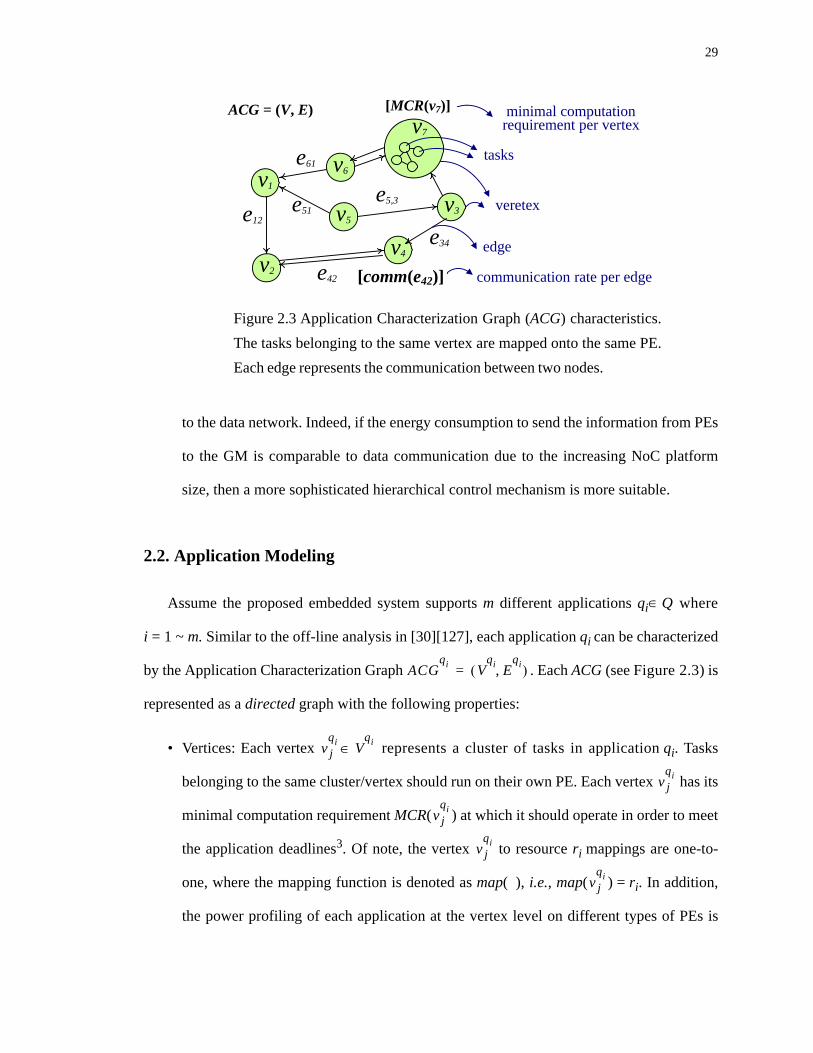
29

to the data network. Indeed, if the energy consumption to send the information from PEs

to the GM is comparable to data communication due to the increasing NoC platform

size, then a more sophisticated hierarchical control mechanism is more suitable.

2.2. Application Modeling

Assume the proposed embedded system supports m different applications qi Q where

i = 1 ~ m. Similar to the off-line analysis in [30][127], each application qi can be characterized

by the Application Characterization Graph . Each ACG (see Figure 2.3) is

represented as a directed graph with the following properties:

• Vertices: Each vertex represents a cluster of tasks in application qi. Tasks

belonging to the same cluster/vertex should run on their own PE. Each vertex has its

minimal computation requirement MCR( ) at which it should operate in order to meet

the application deadlines3. Of note, the vertex to resource ri mappings are one-to-

one, where the mapping function is denoted as map( ), i.e., map( ) = ri. In addition,

the power profiling of each application at the vertex level on different types of PEs is

∈

ACGqi V

qi Eqi,( )=

Figure 2.3 Application Characterization Graph (ACG) characteristics.The tasks belonging to the same vertex are mapped onto the same PE.Each edge represents the communication between two nodes.

veretex

tasks

communication rate per edge

ACG = (V, E)

e12

[comm(e42)]

e51

v1

v2

v3

v4

v5

e5,3

e34

v6e61

edge

v7

e42

[MCR(v7)] minimal computation requirement per vertex

v jqi V

qi∈

v jqi

v jqi

v jqi

v jqi

30

assumed to be available where represents the power

consumption, while vertex maps/executes on resource rk. Of note, for some

memory intensive applications, e.g. multimedia, a vertex can also be characterized as a

buffer or memory unit and needs to assign to the corresponding memory block in the

platform (see Footnote 2 in this chapter).

• Edges: Each directed edge in E characterizes the communication between

vertex and vertex , while weights comm( ) stand for the communication rate

(i.e., bits per time unit) from vertex to vertex .

2.3. Trace-based Energy Modelling

Multiprocessor embedded computing systems are always designed with the goal of

consuming less power. The trend of adding heterogeneity helps low the power demands while

maintaining performance. For a reasonable platform modeling, as seen in Section 2.1, we

have n different types of PEs with different computation capabilities in our NoC platform.

Here, a system-level energy modelling for such NoC-based MPSoC platform is presented. It is

worth to mention that as reported by the MIT RAW on-chip network, the communication

energy consumption represents 36% of the total energy consumption [20]. Therefore, in order

to achieve the accuracy of the high level system modeling, our proposed energy model covers

both computation and communication modules. We first formulate the user traces which are

recorded from relevant users over time and then describe for the computation energy model

and communication energy model, respectively, for such trace-based user patterns.

3.Note that, while dealing with the off-line task partitioning process, in order to meet the applicationdeadline, we use the worst case communication time for communications between nodes (i.e., lon-gest communication path). Moreover, we use the worst case execution time (WCET) for data-dependent tasks, where the WCET of a task is the maximum length of time that the task takes toexecute on a resource with certain computation capability.

P vjqi rk map vj

qi

⎝ ⎠⎛ ⎞=,⎝ ⎠

⎛ ⎞

vjqi

ejkqi E

qi∈

vjqi vk

qi ejkqi

vjqi vk

qi

31

2.3.1. User Trace Modeling

As we mentioned in Section 1.3.2, the best way for collecting the user traces is either from

the product prototype or from products belonging to an earlier generation of systems.

However, since such NoC-based products are rather difficult to have access to, we collect user

patterns/traces by monitoring the behavior of the Windows XP environment as users login and

logoff the system. By collecting real traces, as opposed to generate some traces based on

traditional distributions like heavy-tailed or exponential distribution, we are able to directly

capture the essence of human behavior while users interact with computing systems.

Before explaining the collected user traces, some terminology needs to be introduced. Let

[t1, App Q, t2] characterize an event where an application Q enters and then leaves the system

during a specific time period between two arbitrary moments in time t1 and t2. A session is a

sequence of events between a user signing in and out of a system. An episode is a discrete

period extracted from a session. The behavior of any user is defined as a set of consecutive,

overlapping events spanning a given period of interaction between the user and the system. In

order to learn the user’s behavior, it is desirable to examine long episodes, or even entire

sessions, as this would generate more accurate user data.

In our experiments, we collect multiple sessions from twenty users within three months.

Each session is represented as discrete time sequences sampled in 10 minutes4

collecting from user i while logging the system. Each element = {q1, q2,...} represents a set

of applications actively running in the system at discrete time t. For example, from the session

of user i,

4. Here we set 10 minutes for sampling the collected user traces at application-level with the consider-ation of reasonable simulation time for our experiments. For obtaining more accurate user interac-tion with the system, it is suggested to sample at higher rates, e.g. every minute, or to collect data atthread- or process-level.

ℜi ℜit⟨ ⟩=

ℜit

32

(2.1)

it is intuitive to see that at time 2, applications 2 enters the system and leaves at time 5.

Application 1 enters the system at time 1 and leaves at time 3, but later enters again at time 4,

etc. We can further obtain several events from this session, e.g. [1, App 1, 3], [2, App 2, 5], [4,

App 3, 8], [6, App 2, 7].

Therefore, by doing such an experiment, the collected information includes the detailed

time sequence of applications usage in the system; that is, we understand that “when

considering how many and which applications the user frequently accesses and for how long”.

Those traces will be utilized for later experiments discussed in Chapter 4 and Chapter 7.

2.3.2. Computation Energy Modeling

represents the computation energy consumption while running α onto

{β}, where α can be a vertex vi, an application qi, or a user trace , and {β} stands for a

resource set with one or multiple number of available resources able to run α. Assume

that the power consumption of each task running on certain specific resource is obtained

by off-line analysis and given in advance (as explained in Section 2.2),

can be obtained as a linear summation of the computation cost of running each vertex onto

the corresponding resources. Assume the duration of the trace α is from time 0 to ,

(2.2)

where is 1 if vertex vi is running on the system, 0 otherwise. Through this

dissertation, we are using embedded benchmark suite from [50] which profiled the codes

ℜi ℜi1 ℜi

2 ℜi3 ℜi

4 ℜ5, , , , i ℜi6 ℜi

7 ℜi8 …, , , ,⟨ ⟩=

q1{ } q1 q2,{ } q2{ } q1 q2 q3, ,{ } q1 q3,{ } q2 q3,{ } q1 q3,{ } q2{ }…, , , , , , ,⟨ ⟩=

Ecomp α β{ },( )

ℜi

Ecomp α β{ },( )

Tα

Ecomp α β{ },( ) P viqi rk map vi

qi

⎝ ⎠⎛ ⎞=,⎝ ⎠

⎛ ⎞ Δvi t( )

t 1=

Tα

∑⎝ ⎠⎜ ⎟⎜ ⎟⎛ ⎞

×vi in app qi or trace ℜi∀

∑=

Δvi t( )

33

of real embedded applications from EEBMC benchmarks (available at www.eembc.org)

onto several commercial processors and reported the power profiles for each vertex and

the corresponding graph for application qi, as well as the idle power for

each commercial processors.

2.3.3. Communication Energy Modeling

The communication energy modeling for NoC architectures have been explored in the

literature [170]. Ye et al. in [170] built the bit energy metric (with bit-level accuracy) for

modeling the energy consumption in a communication network. More precisely, it tracks

the dynamic energy consumed when transmitting one bit of data from the source to the

destination PEs through the whole network fabrics, including interconnect wires, arbiters,

input/output buffers, and crossbar for routing the data.

In this dissertation, we choose the bit energy model from [170] as it provides an efficient

approximation for the network fabrics under consideration with reasonable accuracy in

system-level of abstraction. For transmitting one bit through each network fabric component

(interconnect wires, buffers, etc.), we obtain the parameters from the Predictive Technology

Model (PTM) [129] which provides accurate, customizable, and predictive model files for

future transistor and interconnect technologies. We believe that with PTM, the modeling of

the system interconnect is accurate enough even before the advanced semiconductor

technology is fully developed. Here, we give the details of the communication energy

modelling for our NoC platform supporting worm-hole switching and minimal-path routing.

represents the total communication energy consumption of running α

(user traces recording the behavior of a set of applications over a finite period of time) on

the resource set {β} from time 0 to (the duration of user trace α), while vertices having

higher communication are assigned to PEs as closely as possible:

ACGqi V

qi Eqi,( )=

Ecomm α β{ },( )

Tα

34

(2.3)

where = 1 if application Q is active in the system between time t-1 and t, and

0 otherwise. The communication energy consumption of any application Q per time unit is

calculated as follows:

(2.4)

where is the communication rate of an edge in application Q (in bits per time unit),

and stands for the energy consumption to send one bit between the PEs where

vertices vi and vj are allocated to (in Joules per bit). More precisely,

(2.5)

The term represents the Manhattan Distance between the PEs where vertices vi and

vj are allocated to. The parameter stands for the energy consumed in routers, including

the crossbar switch and buffers, while represents the energy consumed in one unit link,

for one bit of data; these parameters are assumed to be constant obtained from the PTM

model.

We note that the parameters and would be different due to different circuit

design, post-silicon devices, wirelength and bandwidth, or even under different semiconductor

technology [129]. Here, we set them as fix values such that the overall computation and

communication energy consumption ratio is about 7:3, similar to the observation from the

MIT RAW on-chip network [20].

Ecomm α β{ },( ) EcommApp Q ΔApp Q t( )

t 1=

Tα

∑⎝ ⎠⎜ ⎟⎜ ⎟⎛ ⎞

×all applications

∑=

ΔApp Q t( )

EcommApp Q comm eij( ) EBit eij( )×

eij∀ E in App Q∈∑=

comm eij( )

EBit eij( )

EBit eij( ) MD eij( ) 1+( ) ERbit× MD eij( ) ELink×+=

MD eij( )

ERbit

ELink

ERbit ELink

35

3. SYSTEM INTERCONNECT DSE FOR FULL-CUSTOM NOC

PLATFORMS

3.1. Introduction

In the foreseeable future, it is expected that more computing resources will be integrated

into systems built at nanoscale. Consequently, the interconnect infrastructure plays a crucial

role for building truly scalable platforms [28]. For application-specific multi-processor

systems-on-chip (MPSoCs) supporting one or a few dedicated applications resulting in

predictable system configurations, customizing the computation and communication

architecture is needed in order to optimize various design metrics, such as power

consumption, throughput, area overhead, wirelength cost, etc.

Interconnect topology and protocol design are both critical steps while designing the chip

communication infrastructure. We note that most of the existing interconnect solutions are

developed to support a specific standard or in-house communication protocol [75]. In this

chapter, we propose a new approach which improves the system interconnect for data

transmission, while leaving the protocol untouched. This facilitates design re-use and

minimizes the design effort which are all critical to meet the tight time-to-market constraints.

Starting from these considerations, the goal of this chapter is to develop a new

methodology for system interconnect exploration, that allows designers to easily take

meaningful (system-wide) optimization decisions. More precisely, our approach optimizes the

data communication phase by replacing the bus-based interconnect with a NoC architecture,

while minimally altering the control phase of the communication protocol. In other words,

36

instead of providing a specific interconnect solution which satisfies the imposed design

constraints, the proposed approach explores a class of communication architectures

exhaustively, while considering the available floorplanning information [2][57]. As a results,

our approach can help designers find the Pareto-optimal solutions trading off power,

performance and other design metrics that account for various physical-level effects.

Due to the high resource reuse it enables, this hybrid approach can be easily integrated

into an up-to-date design flow in industry, as opposed to forcing a sudden paradigm change

towards fully NoC-based designs. To the best of our knowledge, this is the first attempt to

implement a hybrid communication model where the data phase (i.e. data transmission)

happens via the NoC approach, while the control phase from the original protocol design is

kept unchanged. Towards this end, our main contributions are as follows:

• The SIDE framework is proposed in an analytical manner for system interconnect

design space exploration, which allows a single run to explore multiple design points

that trade off various design metrics (e.g. average packet latency, area cost, wirelength).

The accuracy of the proposed analytical model is further validated using a SystemC

simulation model specifically developed for this work.

• To reduce the exploration complexity, we also propose a heuristic approach which

achieves three orders of magnitude reduction in runtime, while still providing high

quality solutions compared to the optimal solution.

• By taking the floorplanning information into account while enumerating various system

interconnect topologies, we are able to produce optimal placement of resources across

the communication fabric.

Taken together, these contributions represent an important step towards providing

designers an efficient analytical solution for system interconnect in application-specific

37

MPSoCs. Of note, the terms system interconnect and communication fabric, are used

interchangeably in this chapter.

The remaining of this chapter is organized as follows. In Section 3.2, we review the

related work. The general MPSoC platform with the related interconnect problem and design

space exploration flow are described in Section 3.3, while new optimization algorithms are

presented in Section 3.4. Experimental results in Section 3.5 show the accuracy and efficiency

of our system interconnect exploration under realistic benchmarks and an industrial case

study. Finally, we summarize our contribution in Section 3.6.

3.2. Previous Work

There exists a significant body of work on synthesizing and generating bus-based systems.

For instance, Sonics MicroNetwork [156] is a TDMA-based bus system handling different

access patterns, interrupt schemes of the intellectual property (IP) modules, while still proving

a high bandwidth. The STBus from STMicroelectronics is a flexible and high-performance

communication infrastructure based on shared buses and support for advanced protocol

features, such as out-of-order and multi-threading [160].

NoCs have been recently proposed as a promising solution to solve the scalability problem

in bus-based systems [17][47]. For application-specific NoCs, using the regular topology is

not always a good choice. Instead, topology selection and synthesis are becoming critical steps

in the design of an efficient communication architecture [107][168]. For instance, Yan et al.

propose greedy algorithms with Steiner-tree methods for reducing the NoC synthesis problem

[168]. The NoC synthesis problem considering physical effects, such as floorplanning and

wirelength, is discussed in [18][78][85][108][158]. Ascia et al. propose genetic approach for

NoC mapping problem considering multiple objectives [5]. In addition, other tools, such as

38

xpipes [85], NetChip [18], for NoC architecture automation and interconnect modeling

[9][120][170] are proposed for system-level communication optimization.

3.3. System Interconnect in MPSoC

3.3.1. General Framework for Application-specific MPSoC

Figure 3.1 shows a generic architecture for application-specific MPSoCs. As seen, such a

platform consists of multiple computing modules, i.e. general-purpose processor, graphics

processing units (GPU), Digital signal processor (DSP), intellectual property (IP), i.e. video/

audio processors, and related peripheral Input/Output (I/O) controller. These modules are not

only communicating with each other through the system interconnect, but also connected to

the off-chip memory and I/Os, such as universal serial bus (USB) devices, serial advanced

technology attachment (SATA), universal asynchronous receiver/transmitter (UART),

peripheral component interconnect (PCI).

Figure 3.1 Block diagram for a general MPSoC platform.

AudioProcessor

one or more levels of

cache

CPU

VideoProcessor

DSP

RISC

Others...

Display

system interconnectmemory controller

memory

others…

Wi-Fi

flash

UART

PCI

USB

SATA

Ethernet

Peripheral I/O controller

39

Traditional system interconnect uses the bus-based protocol which consists of two main

phases, namely a control phase and a data phase. A complete data transmission from a source

IP block to a destination block needs to complete the control phase first and only then the data

phase can proceed. The control phase follows the general handshake protocol (with VALID/

READY signals and exchanges of data packet information like data size, data priority etc.) to

ensure that the data are successfully transferred to/from buffer through the up-stream and

down-stream data buses, respectively.

The general platform with multiple IPs connecting with the system interconnect is shown in

Figure 3.2. In this representation, each IP block bi has only one input and one output port

denoted as “ini” and “outi”, respectively. The data packets are sent/received to/from the

communication fabric through the network interfaces. In general, the communication fabric

consists of multiplexers (mux), repeaters for transmitting packets over long links, links of

wire

other control circuits…

data bus

control bus

buffere.g. SRAM (on-chip), DRAM (off-chip)Scratchpad memory (SPM) …

multiplexer

set arbiter

repeater

IP block b0

IP block b2

out0

in0

out 3

in3

out2

in2

out |B

|-1

in|B

|-1

out 1

in1

system interconnect

IP block b|B|-1IP block b3

IP block b1

Figure 3.2 General platform with multiple IPs communicated via thesystem interconnect.

40

different widths, storage elements (e.g., elastic buffer memory, static random access memory,

scratchpad memory, dynamic random access memory, etc.), and other control circuitry (e.g.,

the arbiter). All signals in the control phase are managed by the system arbiter which drives

multiple data transactions and supports out-of-order transaction completion too. In addition,

each IP block of the platform can act as a master, slave, or both under such protocol. A master

initiates read or write (R/W) requests to the arbiter, while a slave can only respond to such R/W

requests from the arbiter. However, such a bus-based protocol is not scalable and becomes

easily a performance bottleneck as the number of IP blocks in the platform increases (i.e. ten-

plus IPs). Therefore, our idea is to keep the control phase (i.e. communication protocol) as it is

and build other communication fabric for data transmission among IPs. In addition, the system

arbiter is not only responsible for handling and scheduling the send or receive requests from

master or slave IP blocks, but also for setting up the path similar to circuit switching

techniques for data transmission on the proposed communication infrastructure. The problem

formulation for system interconnect is discussed next.

3.3.2. System Interconnect Problem Formulation

The system configurations are assumed to be predictable where may derive from one or

multiple use-case applications [105]. Similar to the application modeling in Section 2.2, the

use-case applications are decomposed into a set of communicating tasks via static analysis and

simulation and are characterized by an application characterization graph (ACG) = (V, E),

which is a directed graph where each vertex bi in B represents an IP block, while each directed

edge eij in E characterizes the communication flow from vertex bi to vertex bj. The weights

comm(eij) stand for bandwidth values (in bits per second) required for communication from

vertex bi to vertex bj. The system interconnect problem can be formulated as follows:

41

Given i) Floorplan of the system with information about placement regions or exact

locations for input and output ports, ii) the ACG and iii) design metrics and constraints (e.g.,

wirelength, area, power);

Objective - Explore a class of communication architectures that trades-off the system

performance and other design metrics, while meeting all the imposed constraints (i.e.,

maximum wirelength and communication fabric power-consumption overhead).

The high-level view of the interconnect synthesis problem with |B| = 4 IP blocks is shown

in Figure 3.3. Figure 3.3(a) explore the system interconnect trading off the system

performance and area/wirelength overhead, showing in left and right y-axis, respectively. As

shown, there are two extreme points in the design space. One left-most point illustrates the

system interconnect corresponding to a traditional bus for four IP blocks1: the data can be sent

from any source IP to the up-stream bus and then be stored in the buffers. Later on, once the

destination IP is ready for receiving data, the stored data can be delivered through the down-

stream bus to its destination IP. Such a communication model is simple and typically has a

low area and wirelength overhead (see Figure 3.3(b)). However, such a bus model will suffer

from poor performance and scalability issues when integrating more IP blocks in the system

since all data transmissions need to share the same wires (i.e. the up-stream and down-stream

buses).

Figure 3.3(c) plots the other extreme case, i.e. fully connected switches. Intuitively, the

system performance of such a model is much better than the one in Figure 3.3(b), since each

IP can communicate with any other IP, at any time, through its own mux without sharing it

1. In this chapter, a mux as in Figure 3.3 represents a switch with an arbiter so it has routing capabili-ties.

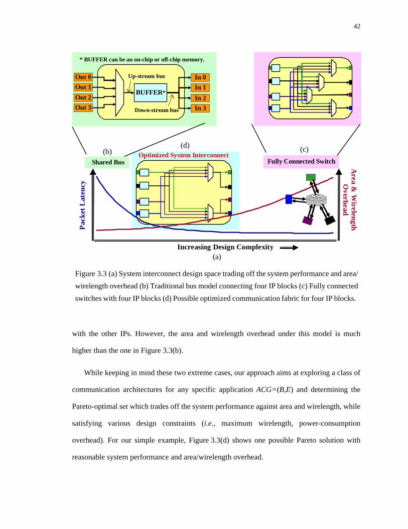
42

with the other IPs. However, the area and wirelength overhead under this model is much

higher than the one in Figure 3.3(b).

While keeping in mind these two extreme cases, our approach aims at exploring a class of

communication architectures for any specific application ACG=(B,E) and determining the

Pareto-optimal set which trades off the system performance against area and wirelength, while

satisfying various design constraints (i.e., maximum wirelength, power-consumption

overhead). For our simple example, Figure 3.3(d) shows one possible Pareto solution with

reasonable system performance and area/wirelength overhead.

Figure 3.3 (a) System interconnect design space trading off the system performance and area/wirelength overhead (b) Traditional bus model connecting four IP blocks (c) Fully connectedswitches with four IP blocks (d) Possible optimized communication fabric for four IP blocks.

Shared Bus

BUFFER*

In 0In 1

In 3In 2

Up-stream bus

Down-stream bus

* BUFFER can be an on-chip or off-chip memory.

Optimized System Interconnect

Pack

et L

aten

cy

Area &

Wirelength

Overhead

Increasing Design Complexity

Out 0Out 1

Out 3Out 2

Fully Connected Switch

(c)(d) (b)

(a)

43

The solution space of this interconnect problem, from a logical view, follows the |B|th Bell

number, also known as the set partitioning problem, where Bn is the number of ways that a set

of n elements can be partitioned into non-empty subsets [13]. For example, B4 = {(1234),

(1)(234), (2)(134), (3)(124), (4)(123), (12)(34), (13)(24), (14)(23), (12)(3)(4), (13)(2)(4),

(14)(2)(3), (23)(1)(4), (24)(1)(3), (34)(1)(2), (1)(2)(3)(4)}, i.e. elements 1, 2, 3, and 4 are

partitioned in 1, 2, 3, or 4 subsets. Also, it is clear that the interconnect in Figure 3.3(b), (c),

and (d) correspond to sets (1234), (1)(2)(3)(4), and (12)(34), respectively.

We note that the solution space grows rapidly, the time complexity being O(nlogn)n (B1-

B10 are 1, 2, 5, 15,..., 115975). In this work, we first propose an algorithm to cover the entire

design space for obtaining the Pareto-optimal solutions (Section 3.4.1); later on, we propose a

heuristic for larger systems to efficiently cover most of the Pareto-optimal solutions as

detailed in Section 3.4.2.

3.3.3. Communication Fabric Exploration Flow

The proposed communication fabric exploration flow for application-specific NoC is

depicted in Figure 3.4. Assume that the floorplan of IP blocks is given2. The inputs of our

flow are i) the I/O port locations (pl) for each IP block, ii) the application communication

graph (ACG) and iii) design constraints, D (e.g., maximum wirelength, maximum power-

consumption for the communication fabric) as shown in Figure 3.4. The modeling block

contains the performance analysis tool, optimal wirelength model in linear-time complexity,

and the fabric area model. Of course, it is also possible to include other models such as, power

[170], or even inductive coupling or crosstalk noise analysis [34] in this exploration.

2. In an industrial setting, this is often the case., e.g., a DDR controller should be near the edge, etc.Moreover, if there are un-placed IP blocks, a floorplanner tool, such as PARQUET [2], can beincluded to floorplan the chip as a pre-processing step.

44

With all inputs and the modeling library available, we explore a class of communication

fabrics and report the Pareto-optimal sets trading off selected design metrics, while satisfying

all design constraints (see the analysis stage in Figure 3.4). Without loss of generality, in the

rest of this chapter we assume that all the communication fabrics work under the same

operating frequency, although the proposed framework can be easily applied to fabrics with

multiple operating frequency settings throughout the chip by reflecting such a concern in the

performance analysis and wirelength models we can handle. In addition, the buffer sizing

problem and specific routing scheme can be further discussed after the communication fabrics

are decided [80][159].

As shown in the simulation stage of Figure 3.4, the netlists corresponding to the Pareto-

optimal sets are automatically generated and fed to the cycle-accurate SystemC simulator

Figure 3.4 The flow of the communication fabric design space exploration withthe analysis, simulation, and evaluation stages shown explicitly.

Constraints (area, power, maxwirelength, ...)

Regions of I/O ports of each IP

App. Comm. Graph (ACG)

Communication Fabric

Design Space Exploration

Evaluation Stage

performanceanalysis model

linear-time wirelength model

other models (power, etc.)

Pareto-optimal solutions

reconfigure mux/ wire connections

traffic generator

SystemC performance simulator with proposed comm. protocal

analysis plot

simulation plot

Simulation Stage

Analysis Stage

netlists

compare

fabric area model

45

specifically developed for this study. The simulator is used both to evaluate the Pareto-optimal

points found analytically and validate the accuracy of our analysis. Our simulator follows the

Intel® XScaleTM System Interconnect (XSI) like communication protocol, on-chip

interconnect for application-specific SoCs, for handling the multiple data transmission.

Finally, we evaluate the accuracy of analytical solutions by simulating them with the SystemC

simulator and comparing the analytical and simulation results, as depicted in the evaluation

stage in Figure 3.4).

3.4. Optimization of System Interconnect Problem

3.4.1. Exact System Interconnect Exploration

Our communication fabric exploration is based on a branch and bound approach. This

approach is capable of searching all solutions efficiently by walking through a tree structure.

For instance, Figure 3.5 shows an example of the tree structure needed to explore the

communication fabric solutions for a simple case with three IPs in the system. Assigning

different IPs to the communication muxes, allows us to explore different solutions. Two

extreme cases of the communication fabric are 1) assign each IP to a separate mux and 2)

assign all IPs to one single mux (see logical views in Figure 3.3(a) and (b), respectively).

As seen in Figure 3.5, the tree structure starts with the root node where no IPs are assigned

to any of muxes. At each level i, we assign IP bi to a different mux, denoted as an intermediate

node, by branching out from its corresponding parent node. For example, the branches of node

(1xx)(xxx)(xxx) at level 2, where IP b2 is placed into muxes 1, 2, and 3, result into nodes

(12x)(xxx)(xxx), (1xx)(2xx)(xxx), and (1xx)(xxx)(2xx), respectively. In addition, to speed up

exploration while keeping the optimality of the approach, we stop branching the nodes which

are isomorphic with other nodes in the tree. For example (see the “R” sign in Figure 3.5), the

46

nodes (1xx)(2xx)(xxx) and (1xx)(xxx)(2xx) are isomorphic, which implies that the solutions

branching out from node (1xx)(2xx)(xxx) are identical to those branching out from node

(1xx)(xxx)(2xx). Therefore, the node (1xx)(xxx)(2xx) is considered redundant in this case and

there is no need to further consider its children nodes in the solution space.

In addition, all nodes at level 3 are leaf nodes since all IPs have been assigned to muxes.

When reaching a leaf node, the expected average packet latency, total wirelength, area, and

power under the resulted mux structure are obtained using our analytical performance model,

optimal tree placer in [32], and the power model. If these results satisfy the design constraints

(e.g., the maximum wirelength in the fabric is smaller than a given value, and the power-

consumption overhead compared to a bus-based design does not exceed a threshold), we

Mux 1

X X X X X X X X X

Mux 2 Mux 3

1 X X X X X X X X

1 2 X X X X X X X

1 2 3

X 1 X X X X X X X

1 X X 2 X X X X X 1 X X X X X 2 X X

1 2 3 1 2 3

Example for 3 IPs

123

123

123

123

- Expected avg. latency- Total wire length- Fabric area

123

12

123

3

123

12

123

3

123

1

123

2

123

3

123

1

123

2

123

3

123

1

123

2

123

3

Level 0

Level 1

Level 2

Level 3

Figure 3.5 A three-IP example of communication fabricexploration using the branch and bound algorithm.

root node

intermediatenode

leaf node

redundant

47

check whether or not this solution belongs to the Pareto-optimal set. If yes, we include the

solution into the Pareto-optimal set and delete any solutions dominated by this one.

The branching process is applied in a recursive manner until all branchings hit level 3 or

stop at some intermediate level. The pseudo code of the branch and bound algorithm

implemented in a depth-first search manner is shown in Figure 3.6. Our solution structure is

listed in lines 01. The main search function of the tree structure is shown in lines 06-21. As

seen, at every iteration, we add one IP to a specific mux (line 06). When reaching a leaf node,

the expected latency, wirelength, area, and power are calculated and the solution is identified

as a Pareto point (lines 12-15). If we reach an intermediate node which is not redundant, we do

Figure 3.6 The pseudo code of the system interconnect explorationusing the branch and bound method.

Input: I/O port regions pl, ACG = (B,E), design constraints D, Output: Pareto-optimal set trading off metrics01 Solution S {latency, area, wirelength, power};02 MAIN PROCEDURE{03 Pareto-optimal ;04 Pareto-optimal = EXPLORE(1, 1);05 } EXPLORE(next_agent, next_mux){06 Solution S[next_mux].push_back(next_agent);07 IF (S is leaf_node)08 S.latency = estimate_latency(S, ACG);09 S.area = calculate_area(S, pl);10 S.wirelength = calculate_wirelength(S, pl);11 S.power = calculate_power(S, pl);12 IF (S satisfies constraints D)13 IF (S dominates solutions in Pareto-optimal)14 Pareto-optimal Pareto-optimal {S};15 delete_non_Pareto in Pareto-optimal;16 ELSE17 FOR (mux_ind = 1 to num_agent)18 IF(S is redundant_node)19 break;20 ELSE21 EXPLORE( next_agent+1, mux_ind ); }

∅←

← ∪

48

the depth-first search recursively to branch out this node by placing the next IP at different

muxes (see lines 17-21).

The estimate_latency function in Figure 3.6 (line 08) computes the average packet latency

for a given solution using a technique similar to the analysis presented in [120]. In short, we

first calculate the contention probability between each flow passing through the same

multiplexer. Then, we use these contention probabilities to find the approximate queuing

delays, as described in [120]. Similarly, the calculate_area and calculate_wirelength functions

in Figure 3.6 (see lines 09-10) are implemented using the technique presented in [32], while the

calculate_power function is estimated under predictive technology model [129].

In summary, for each mux with more than two inputs, we decompose the mux into a tree

structure and later apply the linear time optimal tree placement method in [32] to place each

decomposed mux. After all muxes are placed, the wirelength is calculated using the Steiner tree

method [168]. The corresponding area is the sum of all decomposed muxes, repeaters and

buffers for each mux structure and the corresponding power is the total power consumed on the

system interconnect components.

3.4.2. Heuristic for Speeding up System Interconnect Exploration

The run-time complexity of the above branch and bound algorithm grows exponentially

with the number of IP blocks in the system. Therefore, we propose a linear run-time heuristic

which can obtain solutions close to the ones in the Pareto-optimal set.

For solving the communication fabric optimization problem for |B| IP blocks, we generate

|B| solutions with number of muxes (num_mux) ranging from 1 to |B| (i.e. |B| class). The final

solution of this heuristic is obtained from the best solution among these |B| classes.

49

Figure 3.7 shows one class of the heuristic with two muxes for four IP blocks (i.e., |B|=4,

num_mux = 2). As shown in the figure, the structure starts with the root node where no IPs are

assigned to any mux (see level 0 in Figure 3.7). We first sort the IPs based on the total

communication bandwidth requirement ( ), and assume d1 >

d2 > d3 > d4. Later, at level i, we assign IP block di to each mux, as shown in Figure 3.7; that is,

at level i, we have a partial solution where IPs d1~di are assigned to muxes. Then, we apply

the performance analysis tool (explained in Section 3.4.1) to each intermediate node, i.e.

partial_latency function in Figure 3.7. The algorithm branches only along the node with the

better performance (i.e., lower partial_latency value). In order to deal with the sensitivity to

Mux 1

X X X X X X X

Mux 2Example for 4 IPs

Level 0

Level 1

Level 2

Level 3

X

X X X X X X Xd1 X X X d1 X X XX

branch only node 1 with prob. p if partial_latency(node 2) - partial_latency(node 1) < varpartial_latency(node 1)

d2 X X X X X Xd1 X X X d2 X X Xd1

d3 X X d2 X X Xd1 X X X d2 d3 X Xd1

Level 4 d4 d2 d3d1 d2 d3 d4d1

node 1 node 2

num_mux = 2sort order: d1>d2>d3>d4

node 3 node 4

branch only node 4 with prob. p if partial_latency(node 3) - partial_latency(node 4) < varpartial_latency(node 4)

Figure 3.7 The proposed heuristic for four IPs with the number of muxes set to 2.

intermediate node

leaf node

di comm eij( ) comm eji( )+[ ]j∀

∑=

50

system performance in partial_latency function, we accept the solution with a certain

probability p when its corresponding performance is within the variance var of the best

solution on that level. This process continues until reaching the leaf node (all IPs are assigned

to muxes) and start considering whether or not this solution belongs to the Pareto curve.

3.5. Experimental Results

3.5.1. Industrial Case Study

To evaluate the potential of our communication fabric exploration approach for a real

application, we apply this approach to an industrial SoC design, namely the Intel® media

processor CE 3100 [83]. For this example, we are given the number of IPs in the system, as

well as the application communication graph. In addition, the floorplan information of this

design and the locations of I/O ports for each IP are also known. We used an industrial process

technology for estimating the area, wirelength, and power on system interconnect. Through

system interconnect exploration, we report the Pareto-optimal set trading off performance and

two physical design metrics, i.e., area and wirelength, while satisfying the imposed constraints

such that the system designers can easily make meaningful system optimization choices.

We first apply the proposed exact exploration technique to find the Pareto-optimal set

trading off the average packet latency and communication fabric area (see Figure 3.8(a)) with

the power overhead constraints set to 0.15 (i.e. the power consumption of communication

fabric cannot be more than 15% of that of a bus-based implementation). This makes sense

since the power consumption of the communication fabric does not represent a big portion

from the power consumption of the entire system. Similarly, Figure 3.8(c) reports the Pareto-

optimal set trading off the average packet latency and communication wirelength.

51

In order to validate the accuracy of the analysis stage (see Figure 3.4), we take the

potential solutions in the Pareto-optimal set and simulate them using our SystemC simulator.

The simulation results of data in Figure 3.8(a) and (c) are shown in Figure 3.8(b) and (d),

respectively. Note that in our analysis model (Figure 3.8(a) and (c)), we capture the high-level

system performance without implementing all the details of the communication protocol.

Therefore, the protocol related latencies such as set-up time, is not included in the analysis.

Since the relative accuracy is sufficient to make accurate comparisons between alternative

solutions, we show the normalize latency values in Figure 3.8. We note that the Pareto points

80 85 90 95 100 105 110

0.96

0.98

1analysis

90 100 110 120 130 140 150

0.94

0.96

0.98

1analysis

80 85 90 95 100 105 110

20

30

40

50simulation

90 100 110 120 130 140 150

20

30

40

50simulation

Figure 3.8 System interconnect exploration for a real SoC design. (a) Pareto-optimal set(latency vs. fabric area) obtained via analysis. (b) Simulation results for solutions in (a). (c)Pareto-optimal set (i.e., latency vs. fabric wirelength) obtained via analysis. (d) Simulationresults for solutions in (c).

(a) (b)

(c) (d)

3 muxes

1 mux (bus model)

3 muxes

1 mux (bus model)

3 muxes 3 muxes

1 mux (bus model)1 mux (bus model)

10.2%

5.3%

40%

40%

communication fabric area communication fabric area

wirelength wirelength

1

0.8

0.6

0.4

pack

et la

tenc

yno

rmal

ized

1

0.8

0.6

0.4

norm

aliz

edpa

cket

late

ncy

1

0.8

0.6

0.4no

rmal

ized

pack

et la

tenc

y1

0.8

0.6

pack

et la

tenc

yno

rmal

ized

52

are accurately captured by analysis. Later, in Figure 3.9, we also show that no actual Pareto

points are missed by analysis.

As seen in Figure 3.8, our proposed SIDE framework covers the entire design space

exploration of system interconnect, including the traditional bus model (one mux case or

signal bus) which is suffers from having a poor performance, but involves less fabric area and

wirelength. When compared against the one mux case (i.e. a single bus), the fabric with three

muxes (i.e., the highlighted circles in Figure 3.8) can achieve around 40% reduction in

communication latency with only 5.3% wirelength and 10.2% area overhead with respect to

the original single bus design. The power consumed by the system interconnect with a 3-

muxes implementation is about 8.16% higher than that of a bus-based implementation. Note

that the reported overhead in area and power is negligible with respect to the entire chip area

and power (below 0.1%). However, the communication latency improvement leads to

significant gains in system-level performance for multiple applications.

In addition, we plot the non-Pareto points to confirm that no candidate points are missed

out in our exploration process. After obtaining all solutions with the branch and bound

algorithm, we select forty points with a smaller fabric area and later report the real simulation

90 100 110 120 130 140 150

0.94

0.96

0.98

1

:: Non-Pareto points

Pareto-optimal set

90 100 110 120 130 140 150

0.94

0.96

0.98

1

:: Non-Pareto points

Pareto-optimal set

analysis

90 100 110 120 130 140 150

20

30

40

50

::Non-Pareto pointsPareto-optimal set

simulation

Figure 3.9 Forty non-Pareto points and Pareto curve plots obtained via analysis (a) andvia simulation (b).

(a) (b)communication fabric area communication fabric area

1

0.8

0.6

0.4

1

0.8

0.6

0.4

norm

aliz

ed p

acke

t lat

ency

norm

aliz

ed p

acke

t lat

ency

53

results for those points. The analysis and simulation results for Pareto-points, plus forty non-

Pareto points, are shown in Figure 3.9 (a) and (b), respectively. As shown in Figure 3.9(a), it is

easy to see that all points in the Pareto-optimal set (see cross signs) dominate all other forty

solutions (dot signs). It is worth mentioning that the forty points obtained from the analysis

stage are indeed dominated by the Pareto-optimal set in real simulation, as shown in

Figure 3.9(b); this demonstrates that our early-stage analysis is able to make good design

choices systematically.

3.5.2. Synthetic Applications for Larger Systems

We now evaluate the run-time and the solution quality of the branch and bound approach

(see Section 3.4.1) against the proposed heuristic (see Section 3.4.2). Four categories of

synthetic applications are generated, with complete floorplaning information about I/O

locations for each IP. Each category contains 10 applications with 7, 9, 11, and 13 IPs,

respectively.

Figure 3.10 shows the solutions obtained with the branch and bound approach and our

heuristic (displayed with dots and crosses, respectively) and their corresponding Pareto curves

for one synthetic application with 13 IPs. As seen in Figure 3.10, those two Pareto curves are

close even though three out of Pareto-optimal solutions are not obtained from the heuristic;

that is, points 7, 8, and 14 can be obtained using the proposed heuristic which are indeed in the

Pareto-optimal set (points 1, 2, 6). The degradation in quality of the heuristic solutions

compared to the optimal solutions is calculated as a difference in area between the solution

generated by the heuristic and an area of the Pareto-optimal solution with the closest (from

below) latency. For example, For example, the average area increase with respect to the exact

algorithm for all design points reported in Figure 3.10 is 2%.

54

As mentioned before, the branch and bound exploration is exponential in nature. The run-

time overhead for exploring the system with 7, 8, ... , 13 IPs is 40 ms, 55 ms, 70 ms, 310 ms, 3

s, 2 min, 40 min. For future MPSoCs with hundreds of IPs, there is a need of using the proposed

heuristic to explore the exponentially increasing design space. Figure 3.11 shows how our

heuristic performs compared to the branch and bound approach as the system size grows up

120 140 160 180

0.94

0.96

0.98

1

::::

solutions from branch and bound approachsolutions from heuristicPareto-optimal set (branch and bound) points 1-6Pareto set (heuristic) points 7-14

1

23

45 6

7

8

9

1011 1314

12

Figure 3.10 Solutions comparison between branch and bound methodand the proposed heuristic for system interconnect exploration of asynthetic application with 13 IP blocks.

nor

mal

ized

pa

cket

late

ncy

communication fabric area

1

0.8

0.6

0.4

Figure 3.11 Run-time and solution quality comparison between branch and boundapproach and our heuristic as the system size scales up.

6 8 10 12 140

0.5

1

6 8 10 12 140

1

2

3 x 104

system size (# of IPs) system size (# of IPs)

spee

dup

degr

adat

ion

in q

ualit

y(h

euris

tic/b

ranc

h an

d bo

und)

(bra

nch

and

boun

d/he

urist

ic)

55

(four categories with the number of IP set to 7, 9, 11, and 13). For the heuristic, the parameter

iter, variance var, and probability p are set to 30, 0.3, and 0.5, respectively. For a system

consisting of 11 IPs, our heuristic runs 1800 times faster than the branch and bound algorithm,

on average. Meanwhile, the solutions obtained by the heuristic remain competitive as the

system size scales up.

3.6. Summary

In this chapter, we have addressed the problem of system interconnect exploration for

application-specific MPSoCs where the system configurations are predictable. As a novel

contribution, we have developed an analytical model for network-based communication fabric

design space exploration and theoretically generated fabric solutions with optimal cost-

performance trade-offs, while considering various design constrains, such as power, area, and

wirelength. For large systems, we have proposed an efficient approach for obtaining

competitive solutions with significant less computation time. The accuracy of our analytical

model has been evaluated via a SystemC simulator using several synthetic applications and an

industrial SoC design.

In the remaining of this dissertation, we will address the design space exploration for NoC

platforms where the system configurations are not predictable due to users interacting with

multiple applications within the system.

57

4. USER-CENTRIC DSE FOR HETEROGENEOUS NOCS

4.1. Introduction

As mentioned in Chapter 3, for systems resulting in predictable system configurations, the

traditional Y-chart flow (see Figure 1.3) works well; however, for future embedded systems,

most likely, we will have multiple applications interacting with the system, which results in

unpredictable system configurations. Since such application interaction is due to the end user

behavior, therefore, by analyzing the user interaction with the system, we are able to provide

more robust platforms for applications characterized by high workload variation and

unpredictable system configurations.

In order to consider the end user behavior into the DSE, in this chapter, our user-centric

design methodology relies on collecting user traces from similar, existing systems or

prototypes (see Figure 1.8). The user trace modeling has been discussed in Section 2.3.1,

which captures what applications are running, at what times, in the system. The novel

contributions of our proposed DSE methodology are as follows:

• First, we target user behavior analysis. More precisely, we apply machine learning

techniques to cluster the traces from various users such that the differences in user

behavior for each class are minimized.

• Then, for each cluster, we propose an offline algorithm for automated architecture

generation of heterogeneous NoC platforms that deal explicitly with computation and

58

communication components and satisfy various design constraints, while facing

significant workload variations.

We note that by taking the user experience into consideration into the DSE methodology,

the generated system platforms exhibit less variation among the users’ behavior; this implies

that each system is highly suitable for a particular user cluster and therefore the overhead of

later applying various online optimization techniques can be reduced as well

[36][38][122][152][153]. In this chapter, however, we restrict ourselves to the offline

optimization part of platform generation, while follow up chapters will consider the run-time

optimization aspects (see Chapter 5, Chapter 6, and Chapter 7).

4.2. Related Work

In an early attempt, Dick and Jha propose a multiobjective genetic search algorithm for

co-synthesis of hardware/software embedded systems which trades off price and power

consumption [51]. Some design methodologies for automatic generation of architecture for

heterogeneous embedded MPSoCs were later studied in [7][100]. Different from the heuristics

used to handle a large design space, Ozisikyilmaz et al. propose a predictive modeling

technique to estimate the system performance by looking at information from past systems

[121]. More recently, Shojaei et al. propose a BDD-based approach to efficiently obtain

Pareto points which help multi-dimensional optimization [150]. Instead of using the bus-

based communication, Chatha et al. address the automated synthesis of an application-

specific NoC architecture with optimized topology [31]. However, their approach targets

single application characteristics (i.e., the communication trace graph is fixed) which is

not realistic to use for different users. Murali et al. consider multiple use-cases during the

NoC design process [106]. However, they optimize the NoC using only worst case

constraints. In reality, the distribution of use-cases for various users are very different.

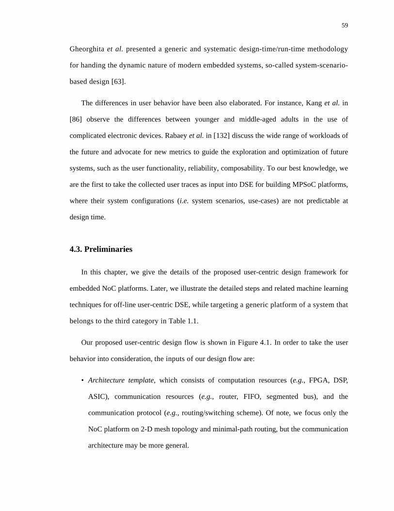
59

Gheorghita et al. presented a generic and systematic design-time/run-time methodology

for handing the dynamic nature of modern embedded systems, so-called system-scenario-

based design [63].

The differences in user behavior have been also elaborated. For instance, Kang et al. in

[86] observe the differences between younger and middle-aged adults in the use of

complicated electronic devices. Rabaey et al. in [132] discuss the wide range of workloads of

the future and advocate for new metrics to guide the exploration and optimization of future

systems, such as the user functionality, reliability, composability. To our best knowledge, we

are the first to take the collected user traces as input into DSE for building MPSoC platforms,

where their system configurations (i.e. system scenarios, use-cases) are not predictable at

design time.

4.3. Preliminaries

In this chapter, we give the details of the proposed user-centric design framework for

embedded NoC platforms. Later, we illustrate the detailed steps and related machine learning

techniques for off-line user-centric DSE, while targeting a generic platform of a system that

belongs to the third category in Table 1.1.

Our proposed user-centric design flow is shown in Figure 4.1. In order to take the user

behavior into consideration, the inputs of our design flow are:

• Architecture template, which consists of computation resources (e.g., FPGA, DSP,

ASIC), communication resources (e.g., router, FIFO, segmented bus), and the

communication protocol (e.g., routing/switching scheme). Of note, we focus only the

NoC platform on 2-D mesh topology and minimal-path routing, but the communication

architecture may be more general.

60

• Applications specification which captures the task graph characteristics (e.g., number of

tasks and communication rate between them), inter-application synchronization,

computation profile (e.g., power consumption, application deadlines).

• User experience which is based on data from users involvement through contextual

enquiry, prototype, and feedback from previous generation products (see

Figure 1.3(b)). This may include user traces, customer preferences, or other relevant

data.

The entire user-centric design flow involves several steps with the goal of generating

systems that meet the user needs. Here, we assume that the user needs in this case are to have

a system with low power consumption, but still able to maintain its basic performance. In

other words, our goal for the system design is to minimize the energy consumption, i.e. the

computation and communication consumption, per user.

Figure 4.1 The proposed user-centric design flow in terms of the off-line DSE processes.

- application charact.- QoS parameters

- comp. components- comm. components - storage elements

- contextual enquiry- prototype- legacy data & feedback

User ExperiencesArchitecture Template Application Template

Automated NoC Platform Design (see Section 3.4.2) 1. Computational resource selection

2. Resource location assignment

...Trace Cluster 1 Trace Cluster 2 Trace Cluster k

NoC Platform 1 NoC Platform 2 NoC Platform k...

Identification Content (IDC)

User Behavior Clustering (see Section 3.4.1) 1. Application usage similarity

2. K-mean clustering process

61

As mentioned in Section 1.3.2, we first need to understand the psychological, social, or

even ergonomic factors that affect the pattern of involvement of different users, in order to

classify the user behaviors. Then, we need to explore the problem of clustering the user traces

such that all users belonging to the same cluster have a similar1 behavior, while interacting

with the target system (see clusters 1 to k in Figure 4.1, details are discussed in

Section 4.4.1). Here, we assume that k is a given design parameter that can be determined by

market surveys or from previous design experience2. After knowing the involvement of users

into the same cluster, we can decide the architecture parameters (i.e., the number and type of

resources) under different design constraints/metrics (area, cost, etc.). Then, for building the

platform, we can follow the NoC platform automation process specific to this cluster of traces

(see Section 4.4.2). Later, we propose a validation process for this user-centric design flow in

order to assess whether or not the system can satisfy the involvement of users in that cluster

configuration (see Section 4.4.3).

To formulate the problem for off-line design, some terminologies are needed:

• ri : a resource of type i considered as the computation component in the platform (see

Section 2.1). Assume there exist n different types of resources, r1, r2,..., rn RE, N(ri)

represents the number of resources of type ri for the platform, while M(ri) represents

the price of resource ri.

• qi : an application with a set of tasks which are not shared with other applications. Each

application qi can be characterized as where the property details of

1. In terms of similar, it can be ‘frequency of accessing an application’, ‘time spent with each particularapplication’, etc. Through confirmatory factor analysis and model analysis, one can derive latentvariables (based on various observable behavior variables as listed above) that can be used to betterclassify users into categories (see the details in Section 4.4.1).

2. For example, for the non-shared systems that owned by certain person, k might be 5 or more, such asthe different models of the cell phones. However, for systems which are shared and used by severalpeople at a time, the universal design (k = 1 or maybe 2) that are usable and effective for everyone issufficient.

∈

ACGqi V

qi Eqi,( )=

62

each application has been described in Section 2.2. Assume there exist m different

applications which can run on the platform, i.e., q1, q2,..., qm Q. Each vertex has a

sets of resources which can only be mapped to in order to meet the application

deadlines, i.e. { } where ri , MCR( ) CC(ri).

We note that the computation/communication energy modeling for a specific user trace

have been characterized in Section 2.3.

4.4. The Problem and Steps for DSE

4.4.1. User Behavior Similarity and Clustering

As mentioned in Figure 1.1, because the variation of user behavior interacting with the

system is quite high and in order to satisfy most of the users through off-line DSE, we need to

classify the user behaviors before clustering the user traces such that the users belonging to the

same cluster would have a similar behavior while interacting with the system. Keeping the

goal of minimizing the energy consumption, we need to observe how users interact with the

system, i.e. how many and which applications the user often uses and for how long. In

addition, each application has different resource requirements and power profiles so extracting

this kind of information is crucial for later customizing the design process.

Here, we define some terms specifically in order to figure out how similar the traces from

users are in a quantitative way; the steps of user behavior clustering process are later explained

in Figure 4.2.

• Application resource demand (L): The degree of resource demands for an application.

The application qi which demands a larger number of resource of type rn has a higher

value.

∈ v jqi

vjqi map 1–⊆ REj

qi ∀ ∈ REjqi v j

qi ≤

Lrn

qi

63

• Inter-application similarity: Two applications requiring similar resources (i.e. having

similar resource demand) have a high inter-application similarity coefficient.

• Application appearance probability ( ): The probability of observing a subset of

applications, v, in user trace .

• Application-usage similarity: Two user traces reflecting a similar frequency of

application appearance (i.e. having similar application appearance probability) have a

high application-usage similarity coefficient.

• Subset function (F): If A is a subset of (or is included in) B, then F(A, B) = 1; otherwise

it is 0.

• Cluster mapping (C): C(i) = j indicates that i has been clustered into the jth group,

where i:C(i) = j represents all the elements in the jth group.

• k-MEAN clustering: The algorithm in [21] groups the objects (or data points) based on

attributes/features into k different groups, where k is a positive integer. The grouping

here is done by minimizing the sum of squares of distances between data and the

corresponding cluster centroid. The k-MEAN clustering algorithm involves three

important steps. First, k initial data points are randomly selected from the data set and

set it as the center if each cluster. Second, we do the re-assign process, i.e. assign other

data points to the closest center. Third, we do the re-center process, i.e. the centroid of

each of the k clusters are re-calculated. We repeat steps 2 and 3 until all these processes

converged (the centroid of each cluster is not changed anymore).

By applying the k-MEAN clustering approach, our goal is to cluster the users having similar

behavior interacting with the system into the same cluster. Each user can be treated as a data

point. The distance between users reflect the coefficient of inter-application and application-

pvℜi

ℜi

64

Figure 4.2 Main steps of user behavior clustering.

Input: task graph characteristics of each application qi , and the task-level computing cost, )Output: user behavior cluster S

• Step 1: Derive the Pareto curve trading off the resources and computation powerconsumption for each application qi (similar to the solution proposed in[51]). Each Pareto point gives the mini-mum power consumption for application qi.

• Step 2: Given all Pareto points, calculate , i.e. the resourcedemand for application qi to each resource type rj for j = 1,..., n, where

• Step 3: Normalize for each application qi.

where

• Step 4: Set each application as a data point di and apply k-MEAN clustering to groupall data points di into z clusters. Assign the center of each cluster, μr where r=1,..., z, to the identification content (IDCr) which will be utilized in the testingstage and define an z-dimensional application vector V = (v1,v2,...,vz) =(di:C(di)=1, di:C(di)=2,..., di:C(di) = z) capturing the applications within thecorresponding cluster.

• Step 5: Calculate for each user trace , i.e. the applicationsets appearance probability with corresponding application set vi for i = 1,..., z,where

• Step 6: Set from traces of each user as a data point di and apply k-MEAN clusteringto group data points di into k clusters. Assign the center of each cluster, μr’,where r’=1, ..., k, to the identification content (IDCr’) and generate a k-dimen-sional trace cluster vector S = (S1, S2, ..., Sk) = (di:C(di) = 1, di:C(di) = 2,...,di:C(di) = k), where Si is a group of user traces with high correlation applica-tion-usage similarity.

• Step 7: Assign μr’ to the identification content (IDCr’). Then, generate a k-dimensionaltrace cluster vector S = (S1, S2,...,Sk) = (di:C(di)=1, di:C(di)=2,..., di:C(di) = k)capturing the user traces within the corresponding cluster.

Gqi T

qi Eqi,( )=

Ecomp tjqi rk,⎝ ⎠

⎛ ⎞

Ecomp qi N r1( ) N r2( ) … N rn( ), , , ,( )

Lqi Lr1

qi Lr2

qi … Lrn

qi, , ,⎝ ⎠⎛ ⎞=

Lrj

qi

∑= =−

−==

))(max(

1 1

1

))]}(,...,)(),...,(,([

))](,...,1)(),...,(,([{j

i

j

rN

x njicomp

njicompqr rNxrNrNqEavg

rNxrNrNqEavgL

Lqi

Lqi Lr1

qi Lr2

qi … Lrn

qi, ,⎝ ⎠⎛ ⎞ Lr1

qi avg Lqi( )– … Lrn

qi avg Lqi( )–, ,⎝ ⎠

⎛ ⎞= =

avg Lqi( ) Lr1

qi Lr2

qi … Lrn

qi+ + +⎝ ⎠⎛ ⎞ n⁄=

Lqi

pvℜi pv1

ℜi pv2

ℜi … pvz

ℜi, , ,⎝ ⎠⎛ ⎞= ℜi

pvj

ℜi

F qk ql,{ } vj,( )qk ql,{ }∀ ℜi

t⟨ ⟩∈∑

ℜit⟨ ⟩∀ ℜi∈∑

pvℜi

------------------------------------------------------------------------------------------------=

pvℜi

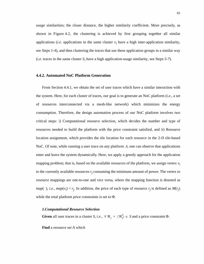
65

usage similarities; the closer distance, the higher similarity coefficient. More precisely, as

shown in Figure 4.2, the clustering is achieved by first grouping together all similar

applications (i.e. applications in the same cluster vi have a high inter-application similarity,

see Steps 1-4), and then clustering the traces that use these application groups in a similar way

(i.e. traces in the same cluster Si have a high application-usage similarity, see Steps 5-7).

4.4.2. Automated NoC Platform Generation

From Section 4.4.1, we obtain the set of user traces which have a similar interaction with

the system. Here, for each cluster of traces, our goal is to generate an NoC platform (i.e., a set

of resources interconnected via a mesh-like network) which minimizes the energy

consumption. Therefore, the design automation process of our NoC platform involves two

critical steps: i) Computational resource selection, which decides the number and type of

resources needed to build the platform with the price constraint satisfied, and ii) Resource

location assignment, which provides the tile location for each resource in the 2-D tile-based

NoC. Of note, while running a user trace on any platform Λ, one can observe that applications

enter and leave the system dynamically. Here, we apply a greedy approach for the application

mapping problem; that is, based on the available resources of the platform, we assign vertex vi

to the currently available resources rj consuming the minimum amount of power. The vertex to

resource mappings are one-to-one and vice versa, where the mapping function is denoted as

map( ), i.e., map(vi) = rj. In addition, the price of each type of resource rj is defined as M(rj)

while the total platform price constraints is set to Φ.

1.Computational Resource Selection

Given all user traces in a cluster S, i.e., S and a price constraint Φ.

Find a resource set A which

∀ ℜi ℜit⟨ ⟩= ∈

66

minimizes (4.1)

such that: Φ (4.2)

vertex vx in S, map(vx) {REx} (4.3)

The steps for the computational resource selection problem are summarized in Figure 4.3.

In Equation 4.2, the sum of the prices of resources integrating in the platform is not

greater the price constraint Φ while Equation 4.3 guarantees that all application tasks

running on the platform would be assigned to the specific resources for meeting the

application deadline.

Main idea: We start out with an initial set of resources (A(0)) which minimizes our

objective without considering the price constraint (Step 1). The price constraints can later

Ecomp ℜi A,( )ℜi∀ S∈∑

⎩ ⎭⎨ ⎬⎧ ⎫

M ri( )ri∀ A∈∑ ≤

∀ ℜi ∈ ⊆

Figure 4.3 Main steps for computational resource selection.

• Step 1: initialize platform A with unlimited resources, find A(0)

which min and j 0.

• Step 2: While ( Θ(j) > Φ)•

find A(j+1) (..., N(rx)-1,..., N(ry)+1,...)

// replace rx with ry,where W(ry) < W(rx), which minimize the energy-price

cost ratio while all tasks still meeting application deadlines, i.e.

and j j+1

End While;

return A(j)

Ecomp ℜi A 0( ),( )ℜi∀ S∈∑

⎩ ⎭⎨ ⎬⎧ ⎫

←

M ri( )ri∀ A t( )∈∑ =

←

min

Ecomp ℜi A j 1+( ),( )ℜi∀ S∈∑ Ecomp ℜi A j( ),( )

ℜi∀ S∈∑–

M ri( )ri∀ A j( )∈∑ M ri( )

ri∀ A j 1+( )∈∑–

-------------------------------------------------------------------------------------------------------------------------------

⎩ ⎭⎪ ⎪⎪ ⎪⎨ ⎬⎪ ⎪⎪ ⎪⎧ ⎫

←

67

be met by replacing the more expensive resources with cheaper ones. Since there are at

most n × (n-1) pairs of possible replacements for a platform with n types of resources,

n × (n-1) evaluations are performed. Then, the replacement that results in the largest price

reduction and smallest computation energy consumption overhead is updated (Step 2) while

satisfying the Equation 4.3 requirement. We continue this step until the price of the updated

resource set satisfies the price constraint.

Example: Assume that we are building a platform with (W × H) = Q resources with the

templates of five different types of resources, i.e. r1, r2, r3, r4, r5 and r1 has the strongest

computational capability but with the highest price. The resource set A is defined as (N(r1),

N(r2), N(r3), N(r4), N(r5)). Under this case, in Step 1 we have A(0) = (Q,0,0,0,0). Then in

Step 2, if A(0)cannot satisfy the price constraint Φ (i.e. Q × M(r1) > Φ), then we replace one

resource with the lower price in the original set, i.e. (Q-1,1,0,0,0), (Q-1,0,1,0,0), (Q-1,0,0,1,0),

(Q-1,0,0,0,1) Find the next iteration resource set A(1) which has lowest price reduction but

with small computational cost overhead. We pursue this greedy approach until finding A(j)

which satisfies the price constraint Φ.

Complexity: Simply speaking, finding the solution space of the computational resource

selection problem is related to that of the integer permutation problem, i.e., finding a

set S = {(N(r1),N(r2),...,N(rn)) | N(r1) + N(r2) + ... +N(rn) = Q}, where the solution

size equals to (Q + n − 1)!/(Q! × (n − 1)!). However, using our proposed greedy approach,

we can obtain a reasonable solution about 60x faster compared to the exhaustive search time

(see experimental results in Section 4.5).

2.Resource Location Assignment

After obtaining the number and type of computational resources from the previous step,

our task becomes to allocate each resource to the tile-based NoC platform with the goal of

N∈

68

minimizing the communication energy consumption when all user traces for a certain cluster

are running in the system. The resource location assignment problem is formulated as follows:

Given all user traces in a cluster S, i.e., S and a W×H 2-D tile-based NoC3

with a resource set A that satisfies

, (W×H). (4.4)

Find a one-to-one resource location assignment Ω( ) from any resource ri in A to a

specific tile location, Ω(ri)=(xi, yi), which

min (4.5)

such that: 1 xi W, 1 yi H. (4.6)

To solve this problem, we need the following notation:

• B(xi, yi): The neighbors of tile (xi, yi), i.e., (xi+1, yi), (xi, yi+1), (xi-1, yi), (xi, yi-1), where

1 xi+1, xi-1 W and 1 yi+1, yi-1 H.

• Empty/Full tile: The tile (xi, yi) without/with a computational resource ri already

assigned to it.

• Transmission matrix ψ: Each entry ψ uv stores the aggregate communication rate

between resources ru and rv.

The steps for the resource location assignment problem are summarized in Figure 4.4.

Main idea: We start out by calculating and normalizing the transmission matrix ψ

(Steps 1-2). Then, by allocating two resources, ru and rv, with the highest ψ uv values as close

3. We believe that the dimensions of the mesh (W × H) or even the total number of resources for build-ing the platform should be determined by previous design experience rather than the outcome of thesynthesis step since it is related not only to system reliability (e.g., one can have spare cores in theplatform), but also to the manufacturing process, or even chip yield. Except for such factors, thevalues of W and H would be close to each other in order to minimize the communication costamong resources.

∀ℜi ℜit⟨ ⟩= ∈

ri∀ A∈ N ri( )i 1=

n

∑ ≤

Ecomm ℜi Ω A( ),( )ℜi∀ S∈∑

⎩ ⎭⎨ ⎬⎧ ⎫

≤ ≤ ≤ ≤

≤ ≤ ≤ ≤

69

as possible, we are able to minimize the communication energy consumption, while running

applications onto the system (Steps 3-5). More precisely, the neighboring resources of ru are

assigned based on the ratio ψui, for i = 1, ..., n, as shown in Step 4.

Complexity: Assume the user trace set is . The exhaustive resource allocation

assignment on a (W × H) = Q platform with the resource set (N(r1), N(r2), ..., N(rn)) is

. (4.7)

Our proposed heuristic can reduce such problem to the complexity of ( ),

where Steps 1 and 2 need to go through the user trace set once before generating

with size k × k. Later, in Steps 3-6, based on , we assign each resource in Q greedily

Figure 4.4 Main steps for resource location assignment.

• Step 1: generate an n×n transmission matrix ψ with each entry

ψ(u, v) = ψ uv =

where map(vj) = ru and map(vk) = rv

• Step 2: normalize the transition matrix ψ,

i.e., ψ uv

• Step 3: get u with largest ψuv or ψvu value, then set the location of ru , i.e. Ω(ru) = (xu,yu), to the center of the platform.

• Step 4: decide B(xu, yu) such that ri with greater ψui has a higher possibility to beassigned to B(xu, yu).

i.e., ψu1 : ψu2 : ... : ψun N(r1): N(r2): ...: N(rn), where r1, r2,..., rn B(xu, yu)

• Step 5: get a filled tile (xu, yu) with the greatest empty neighboring tiles.

• Step 6: repeat Steps 4 and 5, until all resources get assigned to the corresponding tilelocations in the NoC platform.

comm ejkqi

⎝ ⎠⎛ ⎞

ejkqi∀ Y

qi∈

∑qi∀ ℜi

t⟨ ⟩∈∑

ℜit⟨ ⟩∀ ℜi∈

∑ℜi∀ S∈∑

ψuv ψuvv 1=

n∑

⎝ ⎠⎜ ⎟⎛ ⎞

←

≈ ∈

ℜ

ℜ C N r1( )Q C N r2( )

Q N r1( )–× … C N rk( )

Q N r1( )– …– N rk 1–( )–××⎝ ⎠

⎛ ⎞×

ℜ= Q!N r1( )( )! N r2( )( )!× … N rk( )( )!××

---------------------------------------------------------------------------------------×

ℜ ψ Q×+

ℜ ψ

ψ

70

onto the corresponding tile locations in the platform. As shown in experimental results in

Section 4.5, we can obtain a reasonable solution about 4000× faster compared to the optimal

search time.

Of note, we focus only the NoC platform with 2-D mesh (W × H) topology, where W and

H are design parameters which can be determined by previous experience, as explained in

Footnote 3 of this chapter. In addition, minimal-path routing is selected as the switching

scheme through this chapter, but the communication architecture and routing scheme may be

more general. That is, our proposed resource assignment approach can be extended to

different topologies under different routing schemes, for instance, by redefining B(xi, yi)

which are the neighbors of tile (xi, yi) and giving some weight to B(xi, yi) which would capture

the distance (as determined by the topology and routing scheme) among the computational

resources.

4.4.3. Validation Process

Here, we validate the potential and robustness of our user-centric design flow (see

Figure 4.5). In this chapter, the system is defined as robust if it performs well not only under

ordinary/given cases (i.e. training dataset), but also under unpredictable/unknown cases (i.e.

testing dataset). Generally speaking, the training and testing datasets are usually given. The

training dataset is used to generate platforms under the user-centric design flow, while the

testing dataset is used to determine whether or not this design flow produces robust platforms

for different types of users. Theoretically, the user traces (see Figure 4.1) observed from an

older version of the platform, Dbefore, can be set as the training dataset in order to produce a

new generation platform. Then, we should take the user traces running on the new platform,

Dafter, as the testing dataset in order to validate the design flow. However, in practice, we

cannot have access to the later traces, Dafter, in advance. Therefore, if we have a reasonable

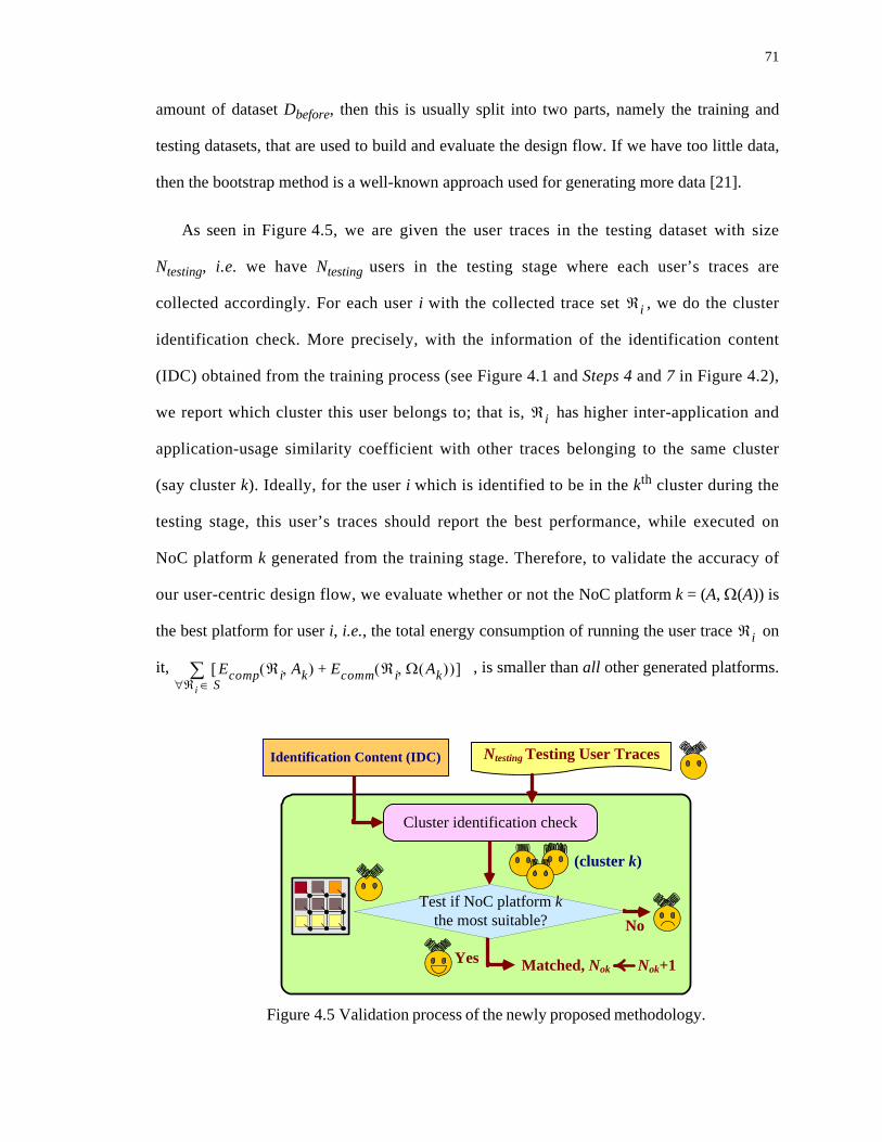
71

amount of dataset Dbefore, then this is usually split into two parts, namely the training and

testing datasets, that are used to build and evaluate the design flow. If we have too little data,

then the bootstrap method is a well-known approach used for generating more data [21].

As seen in Figure 4.5, we are given the user traces in the testing dataset with size

Ntesting, i.e. we have Ntesting users in the testing stage where each user’s traces are

collected accordingly. For each user i with the collected trace set , we do the cluster

identification check. More precisely, with the information of the identification content

(IDC) obtained from the training process (see Figure 4.1 and Steps 4 and 7 in Figure 4.2),

we report which cluster this user belongs to; that is, has higher inter-application and

application-usage similarity coefficient with other traces belonging to the same cluster

(say cluster k). Ideally, for the user i which is identified to be in the kth cluster during the

testing stage, this user’s traces should report the best performance, while executed on

NoC platform k generated from the training stage. Therefore, to validate the accuracy of

our user-centric design flow, we evaluate whether or not the NoC platform k = (A, Ω(A)) is

the best platform for user i, i.e., the total energy consumption of running the user trace on

it, , is smaller than all other generated platforms.

Figure 4.5 Validation process of the newly proposed methodology.

Ntesting Testing User Traces

Yes

Test if NoC platform k the most suitable?

Matched, Nok Nok+1

No

Identification Content (IDC)

(cluster k)

Cluster identification check

ℜi

ℜi

ℜi

Ecomp ℜi Ak,( ) Ecomm ℜi Ω Ak( ),( )+[ ]ℜi∀ S∈∑

72

If yes, it means that the user i passes the validation process and we label it as a match for

user i. Finally, the accuracy rate for our user-centric design flow, i.e., (Nok/Ntesting)×100%,

is reported where Nok is the number of user passes the validation process while Ntesting is the

total number of users in the testing stage. It is obvious that the higher the accuracy rate is, the

more robust the platforms are.


To evaluate the user behavior model and the associated design flow, we apply our

proposed methodology to some real applications with realistic user traces. Our environment

and design inputs are as follows:

• Five different types of computational resources ri are available in the architecture

template; the corresponding processor model and its price (in U.S. dollars, USD), M(ri)

are listed in Table 4.1.

Table 4.1 Architecture template for the NoC platform.

• Seven applications are executed on the system platform, including two synthetic

applications generated by the TGFF package [162], Automotive/Industrial,

Consumer, Networking, Office automation, and Telecom from the embedded system

benchmark suite (E3S) [50]. Some pre-processing (such as task binding,

scheduling) is done for these seven applications, where task graphs have sizes 7, 7,

Resource Type, ri Part Number Price, M(ri)r1: DSP 300MHz TI TMS320C6203 112r2: RISC 266MHz IBM PowerPC 405GP 65r3: DSP 60MHz Analog Devices 21065L 10

r4: x86 μprocessor 400MHz AMD K6-2E 77r5: μcontroller 133MHz AMD ElanSC520 33

73

8, 6, 5, 4, and 6, respectively. Each task is going to execute on one resource later. In

addition, the task profile, the power consumption of running task ti on each

processor type, are analyzed beforehand under specified performance constraints.

• Hundreds of user traces (i.e., both training and testing datasets) are used to validate the

accuracy of the design flow. Realistic user patterns are collected the behavior of the

Windows XP environment from twenty users as users login and logoff the system. We

sample the patterns in about 10 minute for generating the traces; the bootstrap method is

later applied to generate even more traces [21].

Assume that, due to various incompatibilities, at most four applications can execute on the

platform simultaneously. In addition, based on data from market surveys or previous design

experience, assume that our goal is to generate three different platforms (i.e., parameter k is set

to 3) in order to satisfy different types of users. The price constraint for each platform is set to

1500 USD (i.e., Φ = 1500).

4.5.1. Evaluation of User Behavior Clustering

The clustering of user behavior is the most critical step in this design flow. Indeed, if the

user traces in the same cluster have a high variance in terms of the resource requirements, the

corresponding platform may not fit well most users in this cluster.

Figure 4.6 shows the clustering results. All feasible Pareto points are derived trading

off the price of the platform and the computation energy consumption. We randomly

select four users in each trace cluster and plot the corresponding Pareto curves. As shown

in Figure 4.6, the variation of users within the same cluster is quite small. We also

produce three resource sets (A1, A2, and A3) for these three trace clusters, while meeting

the price constraint (Φ = 1500). For example, for cluster 1, the resource set A1 consists of

74

3 resources of type r1, 6 of type r2, 6 of r3, 6 of r4, and 7 of r5, with the total price being equal

to 1479. As shown, these three resource sets (A1, A2, and A3) are quite different although their

prices are close to 1500.

Table 4.2 shows the normalized computation energy consumption of using these three

resource sets with each trace cluster. For example, for the second entry in second column,

the value 1.22 gives the computation energy consumption ratio of running all traces in

cluster 1 onto A1 and A2; that is,

: = 1 : 1.22 (4.8)

1250 1300 1350 1400 1450 1500 15500

1

2

3

4

5

6

7

8

9

10x 109

1250 1300 1350 1400 1450 1500 1550

10

9

8

7

6

5

4

3

2

1

0

x 109

users in cluster1

users in cluster2

users in cluster3

Figure 4.6 Pareto points showing the trade-offs between price and computationenergy consumption. For each cluster, four users are randomly selected and theirPareto curves are plotted.

A1 = (3,6,6,6,7)

A2 = (5,5,3,2,13)

A3 = (3,7,3,4,11)

price (unit: U.S. dollars)

com

p. e

nerg

y co

nsum

ptio

n (μ

J)

Ecomp ℜi A1,( )ℜi∀ S1∈∑


--------------------------------------------------------



--------------------------------------------------------

75

Of note, from Figure 4.6 and Table 4.2, we can conclude that the user-centric

methodology has the potential to separate the users having different behavior interacting

with the system quite effectively. In addition, by doing so, our platforms can be optimized

for each specific cluster of users with the goal satisfied.

Finally, we compare our proposed methodology against the traditional design flow which

generates only one platform, A’ (see the last row of Table 4.2), while optimizing the

computation energy consumption for the entire set of user traces, under the price constraint

Φ = 1500. As it can be observed, we achieve about 30% computation energy savings, on

average, compared to the unique platform, A’, derived from the traditional design flow.

4.5.2. NoC Platform Evaluation

We first evaluate the solution quality of the computational resource selection algorithm in

Section 4.4.2.I for traces with 200 users in the training dataset (Dbefore), against the best

solution which can be derived from the Pareto curve in Figure 4.6. The experiments are

performed on an AMD Athlon™ 64 Processor 3000+ running at 2.04GHz. Compared to

the optimal solution obtained from exhaustive search, our method consumes 5% more

computation energy, on average, for all these three clusters. However, it requires more than

10 hours to get the optimal resource sets for one cluster, while our algorithm takes only about

10 minutes to produce these reasonable platforms. Of note, for evaluating future systems in

Table 4.2 Computation energy consumption comparison for three trace clusters and different resource sets derived by the proposed and traditional design flow.

Resources Traces Cluster 1 Cluster 2 Cluster 3Set A1 1 1.47 1.35Set A2 1.22 1 1.33Set A3 1.33 1.28 1Set A’ 1.50 1.18 1.31

76

the market on millions of users, the proposed heuristic has the potential for producing

platform with industrial time-to-market constraints.

Next, we evaluate the solution quality of the resource location assignment algorithm

(Section 4.4.2.II) against the optimal solution, given a fixed set of resources running the

user traces. We observe that our method consumes only 7% more energy in

communication, on average, compared to the optimal resource location assignment but it

takes several seconds to process our heuristic, while hours for obtaining the optimal

solution.

To show the potential of our approach for larger platforms, we apply our proposed

approach to resource selection and allocation on 6 × 6, 8 × 8, 10 × 10 platforms using the

same settings shown in Table 4.1. Our approach has less than 7% computation energy

overhead and 5% communication energy overhead compared to the optimal solution for these

three platform settings. However, our solution can be obtained within 12, 15, 20 minutes,

while it takes about 40 minutes, 10 hours and more than three days to get the optimal solution

for 6 × 6, 8 × 8, 10 × 10 platforms, respectively.

4.5.3. Evaluation of Entire Design Methodology

Finally, we apply the validation process in Figure 4.5 (Section 4.4.3) to show the

potential of the user-centric design methodology. The size of training dataset ranges from 100

to 700 (we sample the collected user behavior in about 10 minutes as users login and logoff

this system), while the size of the testing dataset is fixed to 500. We observe that the accuracy

rate, (Nok/Ntesting) × 100%, increases as the size of the training data increases (for training

dataset size of 100, 300 and 500, the accuracy rate is 73%, 84%, and 87%, respectively).

By applying 700 training data for building these three platforms, we can have more

77

information for user behavior clustering and therefore, come up with a higher accuracy rate

(around 90%).

4.6. Summary

In this chapter, we have proposed a unified user-centric design framework for off-line

design space exploration (DSE) and on-line optimization techniques for embedded systems.

Our investigations target primarily heterogeneous multi-processor SoCs with resources

communicating via the NoC approach, but the approach is completely general and appropriate

to embedded systems design.

More precisely, in this new design methodology, we consider explicitly the information

about the user experience and apply machine learning techniques to develop a design flow

which aims at minimizing the workload variance; this allows the system to better adapt to

different types of user needs and workload variations. As shown, efficient algorithms have

been proposed for clustering the users’ behavior and automatically generating 2-D NoC

platforms such that the values of the total computation and communication energy

consumption are minimized, give specific design constraints. In addition, a validation process

for the proposed user-centric design flow has been proposed to show the robustness of the

framework. Although we focus on the architectures interconnected by 2D mesh networks with

minimal-path routing schemes, our user-centric design framework can be adapted to other

regular architectures with different network topologies or different deterministic routing

schemes.

Our experimental results using real applications have shown that by considering the user

experience into the design space exploration step, the system platforms generated by our

approach achieve more than 30% total energy savings, on average, compared to the single

platform derived from the traditional design flow; this implies that each system configuration

78

we generate is highly suitable for the targeted class of user and workload behaviors. Last but

not least, the problems addressed in this work are focused at the system-level, while future

work can cover the other levels of abstraction using a similar philosophy.

79

5. ENERGY- AND PERFORMANCE-AWARE INCREMENTAL

MAPPING FOR NOC

5.1. Introduction

Having generated NoC platforms which exhibit less variation among the users’ behavior

in Chapter 4, in this chapter, we concentrate on the dynamic resource management process

and present a robust algorithm for heterogeneous NoC-based MPSoCs. Here, we target real-

time applications described as task graphs (see the application modelling in Figure 2.3) as

opposed to general-purpose best-effort applications usually found in chip multiprocessors

(CMPs). As the target NoC platform discussed in Section 2.1, these applications are mapped

onto embedded MPSoCs where the basic architecture consists of homogenous PEs operating

at multiple voltage levels. More precisely, we assume that only the PEs connected to the NoC

have multiple voltage levels, whereas the network itself (including links, routers, etc.), is in its

own voltage-frequency domain. Of note, our proposed algorithm can also be applied to

platforms with different types of resources without any change with the given CC(ri) for each

resource ri.

A GM is responsible for system resource management which involves mapping the

incoming applications to the available PEs and handling the inter-processor communication

(the details of the control scheme related to GM shown in Section 2.1). Since the arrival order

and execution times of the applications are not known at design time (that is, applications

arrive at arbitrary times and leave the system after being executed), performing effective run-

time mapping is an important and challenging task. Towards this end, we propose a run-time

80

mapping technique which allocates the appropriate resources to the incoming application tasks

such that the communication energy is minimized, given some deadline constraints. At the

same time, all the pre-existing applications still run on the initial set of resources they have

been allocated to.

To illustrate the proposed methodology, we assume a system architecture with two voltage

levels as shown in Figure 5.1. The gray squares represent the PEs operating at higher voltage

levels, while the black dots show the tasks belonging to a pre-existing application which

cannot be reallocated. Applications App 1 and App 2 shown in Figure 5.1(a) and

pre-existing application

greedy solution(cost = 10 + 6 = 16)

proposed solution (cost = 10 + 7 = 17)

+ App

1 + App 2

greedy solution (cost = 10 + 6 + 12 = 28)

proposed solution (cost = 10 + 7 + 8 = 25)

assume (initial cost = 10) + App 2

1 2

4

5

3

76

1

4 5

7

6

23 1

4 5

7

6

23

1 2

4

5

3

76

1

2

3 6

5

4

1

2

3 6

5

4

+ App 1

vertexedge

1

2

5

3

6

4 7

App 1

1

2 5

3 6

4

App 2

Figure 5.1 Example of NoC incremental application mapping comparing the greedy and ourproposed solutions. The greedy approach which does not consider additional mappingsincurs higher communication overhead for App 2, and the system communication cost aswell, compared to our proposed solution.

(a) (b)

(c)

(d) (e)

(f) (g)

81

Figure 5.1(b), respectively, need to be mapped sequentially to the initial system configuration

in Figure 5.1(c). Suppose that vertices 4 and 6 are the critical vertices for App 1, while vertex

2 is the critical vertex for App 2; this means that they must be allocated to the PEs operating at

the highest voltage level in order to meet the application deadlines.

After the arrival of each new application App i, a greedy approach would map App i to the

NoC resources such that the inter-processor communication cost of App i is minimized for the

current configuration (that is, ignoring any future arrivals). In this simple example, the total

system communication cost is the sum of the communication cost of all applications; that is:

(5.1)

where MD(vi , vj) respresents the Manhattan Distance between any two application

vertices, vi and vj, connected to each other. As illustrated in Figure 5.1(d), even though the

greedy approach minimizes the communication cost for the current configuration, the newly

generated region consisting of the remaining (available) PEs is quite scattered. Consequently,

mapping any additional application onto this configuration would be ineffective, as it can be

seen for the non-contiguous region of App 2 in Figure 5.1(e).

As opposed to this, our newly proposed methodology does consider applications that may

arrive to the system at future times and consequently, it offers a more effective mapping in the

presence of dynamically incoming applications. Indeed, as shown in Figure 5.1(g), when

App 2 is mapped after App 1, the system communication cost becomes smaller than the cost

obtained using the greedy approach. Intuitively, since the pre-existing applications cannot be

reallocated, the performance of the greedy solution becomes much worse compared to our

proposed solution.

Note that the task migration approach is complementary to our incremental mapping;

indeed, task migration is an effective strategy to achieve load balancing and high resource

System communication cost MD vi vj,( )

i j,( )∀∑

App∀∑=

82

utilization. For distributed systems without shared memory support, the task migration policy

must be implemented by passing messages among PEs; the implicit migration cost is large due

to the need of moving the process context [19]. However, for embedded MPSoCs with shared

memory, we have two contexts to worry about from a migration perspective: The user context

(called the remote) and the system context (called the deputy or home node). Only the user

context (i.e. stacks, memory maps, registers of the process) needs to be migrated, while the

system context is kept either on the home node or in the shared memory. Therefore, the

migration process can be implemented with middleware support on top of the operating

system. In this chapter, we do not focus on the task migration process. Instead, we target an

incremental mapping process which does not need to change the current system configuration.

In summary, the novel contribution of this chapter consists of a new approach for dynamic

application mapping such that the total communication energy consumption in the system is

minimized. At the same time, additional applications can be easily added to the resulting

system with minimal communication cost overhead.

The remaining of this chapter is organized as follows: We first review the related work

(Section 5.2) and give an motivation example to highlight the key idea of our work

(Section 5.3). In Section 5.4, we formulate the problem of run-time incremental mapping and

present the proposed methodology. Then, we propose a two-step algorithm to solve this

problem; more precisely, the near convex region selection problem is discussed in

Section 5.5.1, while the vertex allocation problem is addressed in Section 5.5.2. The

experimental results appear in Section 5.6, while Section 5.7 summarizes our main

contribution.

83

5.2. Related Work

Resource allocation is a fundamental problem encountered in a variety of areas, including

processor allocation for supercomputers and task assignment in massively parallel processing

systems. While dealing with the resource management process, Karp et al. in [88] study the

problem of finding the shape of a region assigned to tasks for minimizing the pairwise

distance of all points within that region; they observe that there is no closed-form solution for

getting the optimal region. Bender et al. in [14] express the solution as a differential equation

to solve the resource allocation problem and provides a theoretical proof for getting the

optimal solution. Bender et al. in [15] present an approximate algorithm for selecting

processors such that to minimize the average number of communication hops in

supercomputers. Shojaei et al. in [151] present a pareto-algebra heuristic for finding multiple

feasible configurations trading off several design metrics, e.g. energy consumption, with the

resource usage for various types of resources at run-time.

In terms of the off-line resource allocation problem for NoC, several approaches have

been proposed. Hu et al. in [79] propose a branch and bound algorithm to map IP cores onto a

tile-based NoC architecture, while satisfying the bandwidth constraints and minimizing the

total communication energy consumption. The work in [104] considers the mapping problem

for minimizing the communication delay with split routing.

While dealing with the resource management problem for “multiple applications” in the

system, Pop et al. present an approach to incremental design of distributed systems for hard

real-time applications over a bus [130]. More recently, Murali et al. proposed a methodology

for mapping multiple use-cases onto NoCs, where each use-case has different communication

requirements and traffic patterns [105].

84

In terms of the on-line resource management for NoCs, the techniques proposed so far rely

on a resource manager operating under operating system (OS) control [117]. This OS-

controlled mechanism allows the system operate effectively in a dynamic manner. Smit et al.

[154] propose a run-time task assignment algorithm on heterogeneous processors. However,

the task graphs are restricted to have either a small number of tasks or a task degree of no

more than two. More recently, Carvalho et al. propose dynamic task mapping scheme in NoC-

based heterogeneous MPSoCs, targeting the channel load minimization for improving the

performance [27].

As such, all the previous work mentioned above does not maximize the system efficiency

by considering the possible addition of new applications. In this chapter, our goal is to

optimize the communication energy consumption for all possible system configurations (at

different time instances) considering that applications can dynamically arrive and leave the

system.

5.3. Motivational Example

We illustrate the incremental mapping process using three applications. For simplicity, the

system considered in this example has only a single voltage level. As shown in the optimal

mapping solution in Figure 5.2(a), whenever a new application arrives in the system, we

minimize the average communication distance for the incoming application and all existing

applications in the system. Applying the optimal mapping in practice would be infeasible

since the run-time for deciding the configuration which gives the optimal solution and

reconfiguring the previous applications by migrating tasks is too high. However, we can get a

significant insight from analyzing the results produced by an optimal solution. Indeed, by

looking at Figure 5.2, we observe that each application tends to cover a convex region, while

the PE utilization of the system increases. Therefore, if no task migration is allowed,

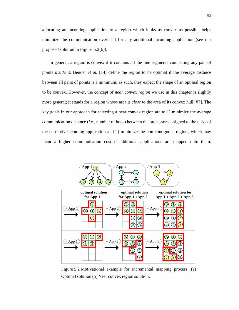
85

allocating an incoming application to a region which looks as convex as possible helps

minimize the communication overhead for any additional incoming application (see our

proposed solution in Figure 5.2(b)).

In general, a region is convex if it contains all the line segments connecting any pair of

points inside it. Bender et al. [14] define the region to be optimal if the average distance

between all pairs of points is a minimum; as such, they expect the shape of an optimal region

to be convex. However, the concept of near convex region we use in this chapter is slightly

more general; it stands for a region whose area is close to the area of its convex hull [87]. The

key goals in our approach for selecting a near convex region are to 1) minimize the average

communication distance (i.e., number of hops) between the processors assigned to the tasks of

the currently incoming application and 2) minimize the non-contiguous regions which may

incur a higher communication cost if additional applications are mapped onto them.

Figure 5.2 Motivational example for incremental mapping process. (a)Optimal solution (b) Near convex region solution.

optimal solutionfor App 1

+ App 1

optimal solutionfor App 1 +App 2

optimal solution for App 1 + App 2 + App 3

+ App 2 + App 3

+ App 1 + App 2 + App 3

2

3

11 24

5

3

1 25

34

1 25

34

1 25

34

1 25

341 24

35

32

41

24

13

2

3

1

32

412

3

1

4

1

2 3 4 5

App 1 App 2 App 31 4

2 3

1 2

3

86

Consequently, our problem formulation generalizes the optimal region considerations [14] for

dynamic system configurations with limited resources.

5.4. Incremental Run-time Mapping Problem

5.4.1. Proposed Methodology

Our proposed methodology is summarized in Figure 5.3. All applications are described

by ACGs which result from an off-line task partitioning similar to [30][127]. Our on-line

incremental mapping process is activated only when an application arrives in the system1. Our

objective is to first select a near convex region (see Section 5.5.1) and then decide on which

PE within this region should each vertex in the ACG be mapped to (Section 5.5.2), such that

the communication energy consumption is minimized under given timing constraints.

1. Of note, in this dissertation, we assume that each application is characterized by one fixed ACG.Therefore, as an application arrives, we realize the number of PEs for selection in order to meetdeadline. However, the application specification could be built more general by considering differ-ent modes of computation. For example, while executing multimedia applications, some users arealways in high-quality mode, but some in low-quality mode under difference situations. This modeprediction can be further captured in the user model, explaining in Chapter 7.

Figure 5.3 Overview of the proposed incremental mapping methodology.

App 2 App n...

Task Partitioning Process

ACGn...

update

System Utilization

(done by GM)

ACG2

on-lineoff-line

Near Convex Region Selection(see Section 5.5.1)

Vertex Allocation(see Section 5.5.2)

App 1

ACG1

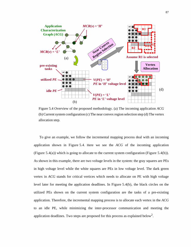
87

To give an example, we follow the incremental mapping process deal with an incoming

application shown in Figure 5.4. Here we see the ACG of the incoming application

(Figure 5.4(a)) which is going to allocate to the current system configuration (Figure 5.4(b)).

As shown in this example, there are two voltage levels in the system: the gray squares are PEs

in high voltage level while the white squares are PEs in low voltage level. The dark green

vertex in ACG stands for critical vertices which needs to allocate on PE with high voltage

level later for meeting the application deadlines. In Figure 5.4(b), the black circles on the

utilized PEs shown on the current system configuration are the tasks of a pre-existing

application. Therefore, the incremental mapping process is to allocate each vertex in the ACG

to an idle PE, while minimizing the inter-processor communication and meeting the

application deadlines. Two steps are proposed for this process as explained below2.

MCR(v) = ‘H’

GM

Assume R1 is selected

idle PE

utilized PE

Application Characterization

Graph (ACG)

GM

R1

R2R3

GM

MCR(v) = ‘L’

PE in ‘H’ voltage level

PE in ‘L’ voltage level

pre-existing tasks

Near Convex

Region Selectio

n

Vertex Allocation

V(PE) = ‘H’

V(PE) = ‘L’

Figure 5.4 Overview of the proposed methodology. (a) The incoming application ACG(b) Current system configuration (c) The near convex region selection step (d) The vertexallocation step.

(a)

(b)

(d)

88

1.The first step is to select a near convex region, that is, to select a region as convex as

possible. The region can be defined as convex if it contains all the line segments con-

necting any pair of its points [87]. That is, as arbitrarily connecting two points in that

region, the line segments should be inside the region. As shown in Figure 5.3(c), R1

and R2 are more convex than region R3; and all of them have at least two PEs at the

high voltage level. Selecting nonconvexity will incur much higher communication costs

for additional mapping. We address this issue in more details in Section 5.5.1. Here, we

assume R1 is selected in this example.

2.The second step consists of assigning vertices to PEs within the selected region (with

critical vertices mapped onto PEs with higher voltage levels), while minimizing the

inter-vertex communication. More details are shown in Section 5.5.2.

5.4.2. Problem Formulation

To formulate this problem, we need a few notations as follows:

• PEij: the PE located at the intersection of the ith row and jth column of the network. We

assume PE11 is the global manager GM3;

• V(PEij): the voltage level that processor PEij belongs to;

• MCR(vi): the minimal computation requirement at which it should operate in order to

meet the application deadlines;

2. For a larger NoC with multiple distributed managers, hierarchical control mechanism may beneeded, similar to the cluster locality approach proposed in [110]. Thus selecting a suitable clusterfor allocating the incoming application would be done before applying our two-step algorithm.

3. Of note, the location of the GM indeed affects the MD of PEs and GM and therefore slightly modi-fies the energy consumption of moving the control messages, as seen in Equation 2.5. However,compared to the energy consumes on sending the data messages, the difference of energy consump-tion on control networks is negligible. Here, we assume the GM is located at the top- and left-mostof the platform.

89

• MD(PEij, PEkl): Manhattan Distance (MD) between PEij and PEkl.

Using this notation, the problem of dynamic incremental mapping for NoCs can be

formulated as follows:

Given the current system behavior and the ACG of the incoming application

Find a near convex region R and a vertex mapping function map( ),

in R, with the objective:

(5.2)

such that .

5.4.3. Significance of the Problem

To prove that the MD metric in the problem formulation heavily affects the

communication energy consumption, we consider the following experiment. An ACG is

generated using the TGFF package [162]. Then we implement four scenarios for mapping this

application onto an 8 × 8 homogeneous NoC. Scenario 1 (S1) in Figure 5.5 uses our method,

scenario 2 (S2) uses the Nearest Neighbor heuristic proposed in [27], scenario 3 (S3)

randomly maps the application vertices inside a 4 × 4 rectangle region, while scenario 4 (S4)

randomly maps the application vertices onto any PEs in an 8 × 8 NoC. The x-axis in

Figure 5.5 represents the average MD between two vertices, while y-axis represents the

communication energy consumption normalized to that of the first scenario. As we can see,

minimizing the MD between application vertices is an effective way to minimize the

communication energy consumption of the applications.

vk∀ V map vk( ) PEij→,∈

min Energy w ei j,( )ei j,∀∑ MD map vi( ) map vj( ),( )×=

⎩ ⎭⎨ ⎬⎧ ⎫

vk∀ V V PEij( ) MCR vk( )≥,∈

90

5.5. Solving the Incremental Mapping Problem

5.5.1. Solutions to the Near Convex Region Selection Problem

When dealing with region selection problem for the incremental mapping process, we

need to minimize the communication cost of the incoming application and, at the same time,

minimize the communication cost overhead for any additional incoming application. To

generalize and formulate this problem, the L1 distance is defined as follows.

Definition 1: The L1 distance of a region R with N tiles, denoted as L1(R), is the total MD

between any pair of these N tiles inside R.

The scenario in Figure 5.6(a) covers the general case of the incremental mapping

problem. Such a scenario includes some pre-existing applications (i.e., the black circles in

Figure 5.6) running in the system, as well as a new incoming application which needs to be

allocated on the remaining/available PEs (these M PEs in the thick line region R are indicated

in Figure 5.6(a)).

0 1 2 3 4 5 6 70

2

4

6

8

Avg. Manhattan Distance between verticesCom

m. e

nerg

y co

nsum

ptio

n ra

tio

Figure 5.5 The impact of Manhattan Distance (MD) on communicationenergy consumption for four different scenarios (S1-S4).

S1S2

S3

S4

91

Assume that this incoming application requires N PEs (with N < M). Our objective is to

find a sub-region R’ with N PEs to assign to this incoming application which minimizes the

metric L1(R’) + L1(R-R’) as shown in Figure 5.6(b)4. Intuitively, it is difficult to consider

these two terms, L1(R’) and L1(R-R’), at the same time. In Section 5.5.1.A, we first focus on

minimizing the first term L1(R’) (we call this the L1 problem), which is a special case of the

general allocation problem. This gives us an insight into the problem of minimizing

L1(R’) + L1(R-R’) which is discussed in Section 5.5.1.B. Finally, in Section 5.5.1.C, the

region selection algorithm is proposed for NoC platforms with multiple voltage levels.

5.5.1.A Minimization of L1(R’)

Minimizing L1(R’) for a region R’ with N tiles is a special case of the general allocation

problem in [15]. To find a lower bound for L1(R’), we first implement the best-case solution to

conjecture the best shape of the region. Then, the worst-case solution in a contiguous region

for this problem is derived as the upper bound. Note that since the incremental mapping

process is done on-line, we need to look for near-optimal solutions with very low cost (i.e.,

4. Of note, if the workload for future applications is predictable, it is suggested to have weights onthese two terms, L1(R’) and L1(R-R’). Such idea is later explored at Chapter 7 while considering theuser behavior into the resource management process.

Figure 5.6 L1(R’) + L1(R-R’) minimization problem: select a region R’, such that the

sum of the total Manhattan Distance (MD) between any pair of tiles inside region R andthat inside region R-R’ is minimized.

(a) (b)

Minimize L1(R’)+L1(R-R’)

Select R’

|R| = M |R’| = N, |R-R’| = M-N

RR＇

R-R＇

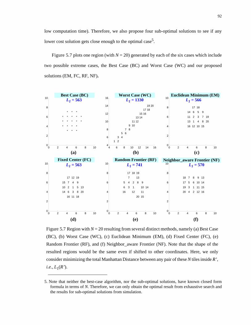
92

low computation time). Therefore, we also propose four sub-optimal solutions to see if any

lower cost solution gets close enough to the optimal case5.

Figure 5.7 plots one region (with N = 20) generated by each of the six cases which include

two possible extreme cases, the Best Case (BC) and Worst Case (WC) and our proposed

solutions (EM, FC, RF, NF).

5. Note that neither the best-case algorithm, nor the sub-optimal solutions, have known closed formformula in terms of N. Therefore, we can only obtain the optimal result from exhaustive search andthe results for sub-optimal solutions from simulation.

0 2 4 6 8 100

2

4

6

8

10Best Case

*

*

*

*

*

*

*

*

*

*

*

*

*

*

*

*

*

*

*

*

4 6 8 10 12 14 164

6

8

10

12

14

16Worst Case

1 2 3 4

5 6 7 8

9 1011 12

13 1415 16

17 1819 20

0 2 4 6 8 100

2

4

6

8

10Euclidean Minimum

1

2 3

4

5 6

7

8

9

10

11

12

13

14

1516

17 18

19

20

0 2 4 6 8 100

2

4

6

8

10Fixed Center

1 2

3

4

5

6

7

8

9

10

11

12

13

14

15

16

17

18

19

20

0 2 4 6 8 100

2

4

6

8

10Random Frontier

1

2

3

4 5

6

7

8 9

10

1112

13

14

15

16

17 18 19

20

0 2 4 6 8 100

2

4

6

8

10Neighbor_awared Frontier

1

2

3

4

5 6

7 8 9

10

11

12

13

14

15

16

17

18

19

20

Neighbor_aware Frontier (NF)Random Frontier (RF)Fixed Center (FC)

Euclidean Minimum (EM)Worst Case (WC)Best Case (BC)

Figure 5.7 Region with N = 20 resulting from several distinct methods, namely (a) Best Case(BC), (b) Worst Case (WC), (c) Euclidean Minimum (EM), (d) Fixed Center (FC), (e)Random Frontier (RF), and (f) Neighbor_aware Frontier (NF). Note that the shape of theresulted regions would be the same even if shifted to other coordinates. Here, we onlyconsider minimizing the total Manhattan Distance between any pair of these N tiles inside R’,i.e., L1(R’).

L1 = 563 L1 = 1330 L1 = 566

(a) (b) (c)

L1 = 563 L1 = 741 L1 = 570

(d) (e) (f)

93

1. Best Case (BC): This corresponds to the optimal solution generated by an exhaustive

search but obviously this works only for moderate values of N.

2. Worst Case (WC): The closed-form solution for the worst-case of a contiguous region

R with N tiles:

L1(worst) (5.3)

Proof: The worst case of L1(R) with N tiles inside R is to place the fth tile to the resulting

region with distance N-k from the kth placed tile where f = 1 ~ N and k = 1 ~ f-1; that is,

L1(worst)

3. Euclidean Minimum (EM): While adding the fth tile into the region with f = 1 ~ N, the

EM heuristic updates the center, (xc , yc), by recalculating the arithmetic mean of f-1 tiles and

then selects a tile (x , y) with minimum Euclidean distance, , to the

updated center.

4. Fixed Center (FC): The 1st tile of the region is always set as the fixed center, (xc , yc).

While adding the fth tile into the region with f = 1 ~ N, the FC heuristic selects a tile (x , y)

with minimum Manhattan Distance, , to the fixed center.

5. Random Frontier (RF): While adding the fth tile into the region with f = 1 ~ N, the RF

heuristic randomly selects a tile from the frontier of the region consisting of N-1 tiles.

6. Neighbor-aware Frontier (NF): Every tile has four neighbors. The tile is considered to

be available, if it has not been selected into the region. While adding the fth tile into the region

R( )N N 1–( )× N 1+( )×

6----------------------------------------------------=

R( ) 1( ) 1 2+( ) … 1 2 … N 1–+ + +( )+ + +=

1( ) N 1–( )×= 2( ) N 2–( )× … N 1–( ) 1( )×+ + +

i N i–( )×i 1=

N 1–∑=

N N 1–( )× N 1+( )×

6----------------------------------------------------=

x xc– 2 y yc– 2+

x xc– y yc–+

94

with f = 1 ~ N, the NF heuristic searches the frontier of the resulted region and then selects a

tile with minimal number of available neighbors.

We should note that there exists more than one solution for these four cases (EM, FC, RF,

and NF), even for the BC and WC scenarios. Figure 5.7 shows a few concrete instances of

regions generated by each of the six cases for N = 20. The numbers on tiles in Figure 5.7(b)-

(f) represent the selection order when forming the regions. We initially set the tile (5, 5) as the

1st tile of the region.

As can be seen in Figure 5.7(a), the resulting shapes of BC are almost “circular”.

However, this solution cannot be applied to run-time incremental mapping due to its high run-

time overhead. For example, it take more than 40 minutes to get the optimal solution for

N = 20, while running on a Intel® Pentium 4 CPU with 2.60GHz. On the contrary, the EM,

FC, and RF heuristics take less than 10 μsec. We observe that for EM and FC cases, they

differ by less than 1% compared to the optimal solution (see Figure 5.7(c) and (d)). For the

RF case, there may exist holes inside the region and this would greatly increase the L1 distance

(e.g., for N = 20, 31.6% increase of the L1 distance compared to the optimal solution in

Figure 5.7(e)). In order to reduce the probability of getting holes inside a region, we propose

the NF heuristic which includes the neighbors information. Indeed, the solution produced by

the NF for N = 20 is only by 1.24% away compared to the optimal solution and it can be

obtained within 5 μsec.

To show the scalability of these heuristics, we need to test regions containing a large

number of tiles. The simulation results for the L1 distance under BC, and WC scenarios and

these four heuristics (EM, FC, RF, and NF) are shown in Figure 5.8(a). We plot the L1

distance from running 1000 experiments with N varying from 1 to 200 (see Figure 5.8(a)).

Since it takes more than 40 minutes to get the result for the BC if N = 20, we do not report

95

results for BC scenario when N is greater than 20 tiles. We do show, however, results for BC

when N varies from 1 to 20 (see Figure 5.8(b)).

From Figure 5.8(a), we observe that the results obtained from EM and FC cases are close

to each other. Of note, the NF heuristic has only 2.63% increase of the L1 distance compared

0 5 10 15 200

100

200

300

400

500

600Worst CaseEuclidean MinimumFixed CenterRandom FrontierNeighbor_aware FrontierBest Case

Figure 5.8 L1 distance results showing the scalability of the solutions obtained via the Best

Case (BC), Worst Case (WC) and four heuristics (EM, FC, RF, and NF).

0 50 100 150 2000

0.5

1

1.5

2 x 105

Worst CaseEuclidean MinimumFixed CenterRandom FrontierNeighbor_aware FrontierBest Case

L 1 d

ista

nce

# of tiles, N

L 1 d

ista

nce

# of tiles, N

(a)

(b)

96

to the FC heuristic for N = 200. Moreover, from Figure 5.8(b), EM, FC, and NF cases are

close to the optimal solution (i.e., the BC scenario) for N varying from 1 to 20.

5.5.1.B Minimization of L1(R’) + L1(R-R’)

Now we have a better sense about minimizing L1(R’) + L1(R-R’). Considering the system

configuration in Figure 5.6(a)), assume that the new incoming application has 12 vertices,

i.e., |R’| = 12. To minimize L1(R’) + L1(R-R’), we implement the EM, FC, and NF heuristics

described above. The first tile of each approach is selected from any boundary tile of R, i.e.

any boundary of the available tiles or next to the boundary of existing vertices. Note that

compared to the problem discussed in Section 5.5.1.A, the L1(R’) + L1(R-R’) minimization

problem has one obvious limitation: the boundary constraint. Under this limitation, for the

EM, FC, and NF cases, we need to add one more constraint; that is, the grid which is selected

should be inside the region R. Additionally, for the NF case, since the boundary condition

greatly influences the neighboring information, we need additional modifications. Initially,

every tile in the grid has four neighbors, except the corner tiles which have only three

neighbors. Other steps are the same as in Section 5.5.1.A.

Figure 5.9 shows the histogram of [L1(R’) + L1(R-R’)] values derived from 1000 runs for

each heuristic (EM, FC, and NF). For example, in Figure 5.9(c) which uses the NF approach,

we can get the [L1(R’) + L1(R-R’)] distance equal to 498 for 369 times. Of note, neither EM

nor FC can obtain this small value. We also summarize these data in Table 5.1 which lists the

L1 distance of the selected region R’ and the remaining region R-R’ for an average of 1000

runs. Also, we list the standard deviation over the mean of L1(R’) + L1(R-R’) in 1000 runs, and

the best/worst results for each heuristic.

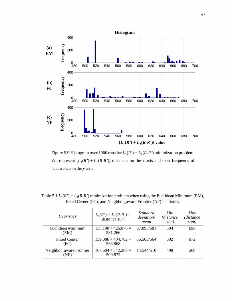
97

Table 5.1 L1(R’) + L1(R-R’) minimization problem when using the Euclidean Minimum (EM), Fixed Center (FC), and Neighbor_aware Frontier (NF) heuristics.

Heuristics L1(R’) + L1(R-R’) = distance sum

Standarddeviation/

mean

Min(distance

sum)

Max(distance

sum)Euclidean Minimum

(EM)155.190 + 426.076 =

581.26667.095/581 504 696

Fixed Center (FC)

159.086 + 404.782 = 563.868

55.503/564 502 672

Neighbor_aware Frontier (NF)

167.604 + 342.268 = 509.872

14.544/510 498 568

Figure 5.9 Histogram over 1000 runs for L1(R’) + L1(R-R’) minimization problem.

We represent [L1(R’) + L1(R-R’)] distances on the x-axis and their frequency of

occurrence on the y-axis.

480 500 520 540 560 580 600 620 640 660 680 7000

200

400

480 500 520 540 560 580 600 620 640 660 680 7000

200

400

480 500 520 540 560 580 600 620 640 660 680 7000

200

400

Histogram

[L1(R’) + L1(R-R’)] value

freq

uenc

yfr

eque

ncy

freq

uenc

y

(a)EM

(b)FC

(c)NF

98

From Figure 5.9 and Table 5.1, we observe that the EM and FC do not work well for

solving the L1(R’) + L1(R-R’) minimization problem. As seen in Table 5.1, even though the

value of L1(R’) of EM and FC heuristics is quite small, the pairwise distance outside the

region, namely L1(R-R’), is relatively high; that is, the selected region does not help for

additional mappings. On the contrary, the NF with the neighboring information included helps

the additional mappings (the decrease in L1(R-R’) distance is 19% and 15% compared to the

EM and FC, respectively). Even if the distance L1(R’) of the NF is about 8% and 5% larger

than that of the EM and FC, respectively, the total distance, L1(R’) + L1(R-R’) of the NF is still

10% less than the solutions provided by the EM and FC. In addition, when observing the NF

in Figure 5.9(c), we have a higher probability to get the smaller L1(R’) + L1(R-R’) value

compared to EM and FC heuristics shown in Figure 5.9(a) and (b). This matches the goals of

the incremental mapping process, namely, to minimize the inter-processor communication cost

for the incoming application (i.e., smaller L1(R’)) and easily add additional applications to the

resulting system with minimal inter-processor communication overhead (i.e., smaller L1(R-

R’)).

5.5.1.C Solution to the Region Selection Problem for Run-time Incremental Mapping

Process

From the discussion in Section 5.5.1.A and Section 5.5.1.B, we decide to apply the NF

heuristic to the region selection problem (see Figure 5.3). Since for the above discussion, all

grids were considered to be the same (i.e., homogeneous system), we need to define two new

terms in order to deal with the heterogeneity of our proposed platform (see Figure 5.4(b)).

• Dispersion factor (D): The dispersion factor of a PE, D(PE), is defined as:

D(PE) = C - number of utilized neighbors of that PE (5.4)

99

where C is a constant. For the corner PEs, C = 3; for other PEs inside (including the

boundary), C = 46.

The PEs with the smaller D(PE) value indicate a higher likelihood to be included into

the current region. Indeed, a PE that has most of its neighbors utilized (i.e., PE with a

small D(PE) value), is very likely to be later isolated; then selecting this PE for the

current region helps reduce its dispersion probability.

• Centrifugal factor (C): The PE centrifugal factor, C(PE), is defined as the Manhattan

Distance between any PE and the border of the current region. PEs with the smaller

C(PE) value indicate a high likelihood to be included into the current region. Indeed,

since every PE in a near convex region should be close to the borders of that region, the

PE with smaller C(PE) is better suited for selection to form a near convex region.

Examples of calculation of the Dispersion and Centrifugal factors are shown in

Figure 5.10. PE12, PE13, PE21, PE22, PE23, and PE31 are running pre-existing applications

and considered to be unavailable. The current region is framed with thicker lines. We

6. The reason of not setting C as 2, 3, 4 for corner tiles, boundary tiles, and others is to avoid the higherprobability of keeping selecting all the boundary tiles into the region, such that the formed regionmay lose the convexity.

Figure 5.10 Dispersion and Centrifugal factor calculation example.

GM1

2

3

4

5

6

7

1 2 3 4 5 6 7

current region

C(PE32) = 1

C(PE77) = 7

D(PE34) = 4

D(PE53) = 3D(PE32) = 1

D(PE77) = 3

C(PE53) = 1

C(PE34) = 2

xy

100

demonstrate how to select and bring PEs into the current region, while keeping its shape as

convex as possible. In Figure 5.10, four PEs (PE32, PE34, PE53, and PE77) are selected as

examples for calculating D(PE) and C(PE). For PE32, D(PE32) = 1 since its neighbors PE22,

PE31, and PE42 are unavailable, while C(PE32) = 1 since it has a Manhattan Distance of 1 to

the region boundary. Other three PEs with Dispersion and Centrifugal factors calculation are

shown in Figure 5.10. Since PE with minimum D(PE) + C(PE) value indicates a higher

likelihood to form a near convex region, under the current region, PE32 is more likely to be

selected to become part of the region compared to PE53, PE34, and PE77. The steps of region

selection (similar to maze routing [93]) are used in Figure 5.11. (assuming k voltage levels in

the system and mk is the number of available PEs in the kth voltage level).

Of note, the k value in the platform does affect the convexity of the region selection; the

larger k value is, the less convexity the region it may form. Therefor, if the k value is too close

to the number of PEs in the system, that is, the platform is much heterogeneity, then it is not

suitable to apply the approach proposed in this chapter. However, it is reported that the k value

is much smaller than the number of PEs in the platform due to the circuit (mixed-clock FIFO)

or energy overhead of communicating PEs in different voltage levels. One experiment in [119]

shows that having 3 voltage levels for 5 × 5 NoC (total 25 PEs) for telecom benchmark

Figure 5.11 Near convex region selection algorithm.

Step 1): Assign each vertex v to Si where i is greater than M(v), and sortthem out in non-decreasing order, |S1|≤|S2|≤ … ≤|Sk|.

Step 2): Start with S1, select a PEij with minimum code transfer energy

Step 3): Update the D(PE) and C(PE) for unselected and idle PEs of

Step 4): Repeat Step 3 for the remaining sets.

that set. Select PEij with lowest D(PEij)+ C(PEij) into region. Continue with Step 3 until the number of PEs in the selected region matches the size of this set.

consumption and include into the region.

101

collected from embedded system synthesis benchmark suite (E3S) [50], the energy

consumption is more than four time reduction compared to the single voltage level case, and

smaller than that of 4, 5, or more voltage levels cases. Given the platform with the reasonable

heterogeneity, our region selected by our proposed approach (see Figure 5.11) forms more

convex than other task allocation approach which does not consider the additional mappings,

which has hugh impact on the overall communication cost as proofed in Section 5.5.1.B.

Now, we consider now a simple example and describe our approach step-by-step. The

ACG of the incoming application and system behavior are given in Figure 5.12 ((a) and (b))

where the black dots show the pre-existing applications in the system. The number marked on

Figure 5.12 Incremental run-time mapping process. (a) The ACG of the incomingapplication (b) Current system behavior (c) Near convex region selection process (d) Vertexallocation process.

GM

|SH|=2|SL|=7

GM1 2

3

4

5

6

7

{1} {2}

{3}

{5}

{4}

{6}

{9}

{6} {6}

R1

ACG

MC

R(v 4

) = M

CR(

v 6) =

v2

v1v3

v4 v5

v6 v7

v8v9

R1 is selected

1

2

3

4

5

6

7

GM

R1

v5 v1

v2

v3

v4v6

v7

v8

v9

1 2 3 4

1 2

｀H

＇

3 4 5

5 6 7

1 2

3

4

5

6

7

1 2 3 4 5 6 7 xy

xy

xy

｀H’ voltage level｀L’ voltage level

(a) (b)

(c)

(d)

102

each PE (e.g., {3} on PE32) in Figure 5.12(c) represents the selection order in forming a near

convex region. PEs with the same number show that they are selected into the region at the

same time.

We can see from Figure 5.12(a), that there are two vertices (v4 and v6) with

M(v4) = M(v6) = ‘H’ which are supposed to be mapped onto the PEs at high (‘H’) voltage

level; the other vertices can be mapped onto the PEs in ‘L’ voltage level, namely, |SH| = 2

(SH = {v4 , v6}) and |SL| = 7 (Step 1). Let us start with SH (Step 2), and assume that PE42 is

selected first to become part of the region for minimizing the code transfer energy

consumption (Figure 5.12(c)). Then, PE43 is the second PE selected for the region (Step 3)

since it has the lowest D(PE43) + C(PE43) = 3 + 1 (D(PE43) = 3 because PE33, PE44, and

PE53 are all idle. Comparing this to D(PE44) + C(PE44) = 4 + 2 or

D(PE46) + C(PE46) = 4 + 4, implies that PE43 gets selected). Step 3 terminates since the PEs

in SH are all selected inside the region. Now, we deal with the selection of SL (Step 4). Going

back to Step 3, PE32 is selected since it has the lowest D(PE) + C(PE) = 1 + 1. After that,

PE33 is selected with D(PE33)+C(PE33) = 1 + 1 and then PE41 is selected with

D(PE41)+C(PE41) = 2 + 1. With the same rule, PE51, PE52, and PE53 are selected with the

lowest D(PE)+C(PE)=4. Finally, PE61 is randomly selected among PE61, PE62, PE63, PE34,

and PE54, with all of them getting the same value of D(PE) + C(PE).

5.5.1.D Complexity of the Region Selection Algorithm

In order to determine the time complexity of the region selection algorithm, assume that

the ACG = (V, E) and the system contains a total of n × n PEs organized in k voltage levels,

where |V| < n2. Therefore, |S1| + |S2| + ... + |Sk| = |V|, where Si is the size of vertex set which is

about to be selected for the ith voltage level and m1 + m2 + ... + mk n2, where mi is the

number of available PEs in ith voltage level.

≤

103

In Step 1 of Figure 5.11, calculating the size of PE sets takes O(V) time and the run-time

for sorting them is O(VlogV) if using QUICKSORT. Steps 2-4 need O(m12+m2

2+...+mk2) since in

Step 3, we need to update D(PE)+C(PE) for each PE in a certain set which takes linear time.

The worst-case scenario occurs when only one PE is selected into the region each time. Thus,

the total run time of region selection algorithm is O(n4+VlogV); that is, O(n4) since VlogV <

n2logn2 < n4. However, in Steps 3-4, we can record the frontier of the region and store the

information, D(PE)+C(PE), of this wavefront in a HEAP. Using this data structure, the run-

time for Steps 3-4 is reduced from O(m12 + m2

2 + ... + mk2) to O(S1logS1 + S2logS2

+ ... + SklogSk) = O(VlogV). Thus, the total time complexity of the region selection algorithm

becomes O(VlogV).

5.5.2. Solutions to the Vertex Allocation Problem

After the near convex region is selected, we continue allocating vertices of the incoming

application to the PEs with specific voltage levels in the selected region (see Figure 5.3),

while minimizing the inter-processor communication. To keep track of the vertex allocation

process, we color each vertex white, gray, or black. A gray vertex indicates that it has some

tentative PE locations but its precise location will be decided later. On the contrary, a black

vertex indicates that it has been already mapped onto some PE and this mapping will not

change anymore. All vertices start out being white and may later either become gray and then

black, or become directly black. A PE is set to be unavailable after a black vertex is mapped

onto it.

We define two actions for vertices:

• DISCOVER: This consists of 1) Select available PEs with a specific voltage level for

vertex t and 2) Color vertex t gray; then, vertex t is considered as “discovered”.

104

• FINISH: This consists of 1) Select a specific PE for vertex t such that the distance

between vertex t and its gray or black neighboring vertices is minimized. (Note that if

more than one PE gets the minimum distance, we select the PEij with its D(PEij) closest

to the number of nonblack neighbors of vertex t) and 2) Color vertex t black; then,

vertex t is considered as “finished”.

In short, we first sort vertices into an ordered set using the non-increasing order of their

total communication volume; that is, the higher communication volume a vertex has, the

earlier it is discovered or finished. The vertex allocation algorithm is summarized in

Figure 5.13.

Let us follow now the same example in Figure 5.12. The ACG in Figure 5.12(a) is going

to be mapped onto the region R1 which has been selected in Section 5.5.1.C. The final result is

shown in Figure 5.12(d); Figure 5.14 shows the vertex allocation process step-by-step.

Remember that for this ACG, the smallest vertex set is SH= {v4 , v6}.

Assume now that, based on the total communication volume, the vertex ordered set is {9,

6, 7, 5, 8, 4, 1, 3, 2}. Also, assume that all vertices are initially white (Figure 5.14(a)). We

Step 1): Color all vertices white. Then, start with the first white vertex in

Step 2): IF neighbors of vertex t are neither gray nor black, then do

Step 3): IF neighbors of vertex t are either gray or black, then do FINISH

Step 4): Go back to the first vertex of the ordered set, do Steps 2 and 3 for

Figure 5.13 Vertex allocation algorithm.

Step 5): Repeat Step 4 if there exists any nonblack vertex in the ordered set; otherwise, stop the algorithm.

each nonblack vertex t until the color of any nonblack vertex changes. Then go to Step 5.

for vertex t.

the smallest vertex set based on the ordered set.

DISCOVER for vertex t.

105

Figure 5.14 Vertex allocation process based on the example in Figure 5.12. (a) Initialconfiguration with every vertex white. (b) Vertex 6 is discovered. (c) Vertex 9 is discovered.(d) Vertex 7 is finished and colored black. (e) Vertex 9 is colored from gray to black. (f)Vertex 6 is colored from gray to black (g) Vertex allocation process is done; all vertices arecolored black.

v2

v1v3

v4 v5

v6 v7

v8v9

v2

v1v3

v4 v5

v6 v7

v8v9

v7

v2

v1v3

v4 v5

v6 v7

v8v9

v2

v1v3

v4 v5

v6 v7

v8v9

v7v9

v6

v7v9

v2

v1v3

v4 v5

v6

v8

v2

v1v3

v4 v5

v6 v7

v8v9

v6

v6 v6

3

4

5

6

1 2 3

v9

v6 v6

v9 v9

v9 v9

v9

v9

v9

v7

3

4

5

6

1 2 3

3

4

5

6

1 2 3

3

4

5

6

1 2 3

3

4

5

6

1 2 3

3

4

5

6

1 2 3

v6 v6

v9

v9 v9

v9

v9

v9

v9

v6 v6

v6 ...

v7

v9

v5

xy

xy

xy

xy

xy

xy

v6

v7v9

v2

v1v3

v4 v5

v6 v7

v8v9

3

4

5

6

1 2 3xy

v5

v2 v4

v3

v8

v1

v9

(a) (b) (c) (d)

(e) (f) (g)

106

start with vertex 6, since it has the smallest order among the vertices in SH (Step 1). Since at

this time its neighbors, vertices 5 and 7 (see in Figure 5.14(a)) are white, we DISCOVER this

vertex (i.e., color it gray) and select PE42 and PE43 (because these are the only PE locations at

‘H’ voltage level in region R1) to map it (Step 2); namely, vertex 6 will be allocated onto PE42

or PE43 later (Figure 5.14(b)). Then continuing with Step 4, we go back to the first vertex in

the ordered set. At this moment, the color of vertex 9 changes from white to gray since all

neighbors of vertex 9 are white; we select PE32, PE33, PE41, PE51, PE52, PE53, and PE61 for

it (Figure 5.14(c)). With the following repeat of Step 4, the color of vertices 9 and 6 remains

unchanged. Then, we consider vertex 7; its color changes from white to black directly since

vertices 6 and 9 are gray. We allocate vertex 7 onto PE52 (Figure 5.14(d)) since PE32, PE33,

PE41, PE52, PE53 has the minimum distance with the gray PEs where vertex 6 allocated and

D(PE52) = 3 equals to the number of nonblack neighbors of vertex 7. And then, since there

exists nonblack vertex in the ordered set, we repeat Step 4. Vertex 9 becomes black since its

neighbor, vertex 7, is colored black (Figure 5.14(e)) and we allocate vertex 9 onto the precise

location, PE51 (Figure 5.14(f)). We continue this process until all vertices are colored black

and each vertex is allocated a precise PE location. Figure 5.14(g) shows the final result of

vertex allocation process.

Complexity of the vertex allocation algorithm: The total run time of our algorithm has a

complexity of O(V2+E). This is because the body of the loop (Steps 4-5) executes |V| times,

while reaching at most |V| vertices each time. In addition, since each vertex will be reached at

most two times (i.e., DISCOVER and FINISH), and the adjacency list of each vertex is

scanned only when the vertex is reached, the total time of scanning the adjacency lists is O(E).

107


We first evaluate the impact of the near convex region selection and vertex allocation

steps of the incremental mapping process using synthetic benchmarks (see Section 5.6.1 and

Section 5.6.2, respectively). Then, the overall algorithm with run-time energy overhead

considered is evaluated using synthetic benchmarks (see Section 5.6.3). To show the potential

of our proposed mapping algorithms for real applications, we later apply it to the embedded

system synthesis benchmark suite, E3S [50] (Section 5.6.4).

5.6.1. Evaluation of Region Selection Algorithm on Random Applications

To show that the choice of a near convex region heavily impacts the communication cost

of the incremental mapping process, we consider the following experiment. Several sets of

applications are generated using the TGFF package [162]. The vertex number and the

communication volume are randomly generated according to some specified distributions.

Then, applications are randomly selected for mapping onto the system or being removed from

it. For mapping onto the resulting system while pre-existing application remain fixed, two

different strategies are implemented: 1) A greedy approach minimizing the inter-processor

communication cost of the current configuration but without considering the newly incoming

applications and 2) A near convex region is first selected using the proposed approach and

then the application is optimally mapped onto this region using exhaustive search.

The number of vertices per application ranges between 5 and 10. The system consists of

7 × 7 PEs with PE11 being used as the global manager. The variance of the communication

volume per edge in one application is set arbitrarily between 0 and 106. Initially, there is no

application in the system. The sequence of events in the system is incremented whenever an

application comes to or departs from the system. If the number of idle PEs in the system is

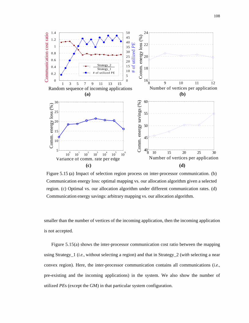
108

smaller than the number of vertices of the incoming application, then the incoming application

is not accepted.

Figure 5.15(a) shows the inter-processor communication cost ratio between the mapping

using Strategy_1 (i.e., without selecting a region) and that in Strategy_2 (with selecting a near

convex region). Here, the inter-processor communication contains all communications (i.e.,

pre-existing and the incoming applications) in the system. We also show the number of

utilized PEs (except the GM) in that particular system configuration.

Variance of comm. rate per edge10

010

110

210

310

410

510

65

10

15

20

25

30

Com

m. e

nerg

y lo

ss (%

)

8 10 15 20 25 3040

45

50

55

60

Number of vertices per application

Com

m. e

nerg

y sa

ving

s (%

)

Figure 5.15 (a) Impact of selection region process on inter-processor communication. (b)Communication energy loss: optimal mapping vs. our allocation algorithm given a selectedregion. (c) Optimal vs. our allocation algorithm under different communication rates. (d)Communication energy savings: arbitrary mapping vs. our allocation algorithm.

0

0.2

0.4

0.6

0.8

1

1.2

1.4

05101520253035404550

:

: # of utilized PE

Com

mun

icat

ion

cost

ratio

1 3 5 7 9 11 13 15Random sequence of incoming applications

Strategy_2Strategy_1 #

of u

tiliz

ed P

E

(a) (b)

(c) (d)

8 9 10 11 1216

18

20

22

24

Number of vertices per application

Com

m. e

nerg

y lo

ss (%

)

109

As shown in Figure 5.15(a), there is a slight increase in the communication ratio at the

beginning because the greedy approach performs well when the number of utilized PEs in the

system is small. Once the number of utilized PEs increases due to the incoming applications,

the benefit of our proposed algorithm becomes obvious. Finally, the ratio becomes stable since

for Strategy_1, when the application leaves the system, there is always a scattered region left

for additional mapping. This example demonstrates that near convex region selection

definitely helps the incremental mapping process.

5.6.2. Evaluation of Vertex Allocation Algorithm on Random Applications

We first compare the run-time and solution of our algorithm against exhaustive approach.

Experiments here are performed on a Intel® Pentium 4 CPU (2.60GHz with 768MB memory),

while we later report the run-time and energy overhead of running our algorithms on the real

embedded processor in Figure 5.6.4. The run-time for finding the optimal mapping within

selected region increases exponentially with the number of vertices in each application: For 8,

9, 10, 11, and 12 vertices in one application, it takes 0.2sec, 1.5sec, 4min, 10min, and 2hrs,

respectively, to obtain the optimal mapping. On the other hand, the run-time of our algorithm

stays within 3μsec, when the number of vertices varies between 8 and 20. Since finding the

optimal mapping for a region with 13 vertices takes more than 26hrs, we vary the number of

vertices per application from 8 to 12 (see points on x-axis in Figure 5.15(b)). More

specifically, there are 5 categories, (|V|=8-12), each category containing 40 applications

generated with TGFF.

We denote the energy consumption of our allocation algorithm by Eh, and the energy

consumption of the optimal mapping with the same region by Ee. Thus (Eh-Ee)/Ee × 100% is

the percentage of reported energy loss compared to the optimal solution. As shown in

Figure 5.15(b), the energy loss for each category is always less than 21%, and not scale up as

110

problem size increases. Therefore, our vertex allocation algorithm provides good results for

large designs.

Now, we address the impact of variance of communication rate per edge on the energy

consumption in Figure 5.15(c). The vertex number in one application used in this experiment

is fixed to 10 and the variance of communication volume per edge is set from 100, 101, 102,...,

to 106 (7 categories). For each category, we run 50 different ACGs and calculate the averages.

It can be seen from Figure 5.15(c) that our average communication energy loss in all

categories is within 21.5% compared to the optimal solution under the same region.

Last, in Figure 5.15(d), we compare the solution of an arbitrary mapping against our

algorithm. Since the run-time of arbitrary mapping is very small, we can consider ACGs with

a large number of vertices (i.e., 30 in Figure 5.15(d)) and see if our algorithm scales well. The

number of vertices per application used in this experiment ranges between 8 and 30 (i.e., 6

categories, |V|=8, 10, 15, 20, 25, and 30). We generate 20 different regions with PE

locations corresponding to the number of vertices in each category and then run 20

different applications on each selected region. The variance of communication volume per

edge and per application is set between 0 and 106.

We denote the energy consumption of our allocation algorithm by Eh, and the energy

consumption of the arbitrary mapping solution by Ea; then (Ea-Eh)/Ea × 100% is the

percentage of reported energy savings compared to the arbitrary mapping solutions which

are averaged from 500 random results. As shown in Figure 5.15(d), at least 45% savings

can be achieved in all categories; of note, the savings increase as the vertex size scales up.

111

5.6.3. Random Applications Considering Energy Overhead for the Entire Incremen-

tal Mapping Process

We compare seven scenarios to our near convex region selection and vertex allocation

technique (denoted as ‘our_all’ in Figure 5.16) in terms of the communication energy

consumption. In this comparison, the communication energy consumption includes the

energy overhead of delivering control messages (see Section 2.1) and that of running our

on-line processes. The latter overhead is measured by executing the C programs on

MicroBlaze processor running on Xilinx Virtex-II Pro XC2VP30 FPGA. For all these

scenarios, we first perform the region selection process using neighbor frontier (NF), euclidian

minimum (EM), fixed center (FC) or our near convex region selection technique (our). Then,

we perform vertex allocation using either random mapping (random) or our proposed

approach (our) presented in Section 5.5.2.

For example, in Figure 5.16, the notation ‘NF + our’ indicates that we implement the

‘NF’ algorithm (in Section 5.5.1.A) for region selection step and then use “our” vertex

Figure 5.16 Communication energy consumption comparisonusing random applications.

0 2000 4000 6000 8000 10000 120000

0.5

1

1.5

2

:::::::

(NF + our) / our_all(EM + our) / our_all(FC + our) / our_all(NF + random) / our_all(EM + random) / our_all(FC + random) / our_all

Total comm. rate per application (bits)

Com

m. e

nerg

y co

nsum

ptio

n ra

tio

Nearest Neighbor / our_all

112

allocation solutions (in Section 5.5.2) for mapping vertices into the selected region. The

experimental results in Figure 5.16 already include the energy overhead of running these

algorithms, i.e., ‘NF’, ‘EM’, or ‘FC’, and ‘our’ where the results in Figure 5.16 assume the

‘random’ algorithm has zero energy overhead.

Finally, the last scenario we consider is the state-of-the-art mapping approach proposed in

[27]. In this case, we allocate the vertices as close as possible without considering a particular

region. The comparison with this scenario is marked as ‘Nearest Neighbor’ in Figure 5.16.

As observed in Figure 5.16, when the total communication rate for applications is too

small, it can be seen the quality loss of our approach due to the comparable run-time energy

overhead of running our mapping algorithm. However, when the total communication volume

per application is over 10000 bits, we can achieve more than 37.5% = (1.6 - 1)/1.6

communication energy savings compared to all other scenarios.

5.6.4. Real Applications Considering Energy Overhead for the Entire Incremental

Mapping Process

The communication energy overhead of on-line processes contains the message

transmission into the control network and our on-line algorithms (i.e., near convex region

selection and vertex allocation). The incremental mapping process is activated only when a

new application arrives, and so the PEs need to send their status to GM. The communication

volume for all control messages is [a bits (for showing PE address, which depends on network

size) + 1 bit (PE status)] × MD (Manhattan Distance of all PEs to GM). For the 6 × 6 network,

a = 6 (26>36), MD = 180; therefore, all control bits for one incoming application are within 1

Kilobit. Compared to the communication volume in real applications (which is in the

Megabits range), the energy overhead for transmitting the control messages is negligible.

113

Next, we evaluate the extra energy overhead of our on-line algorithms. Our system

contains 6 × 6 PEs of AMD ElanSC520 (133 MHz), AMD K6-2E (500MHz), and one

MicroBlaze core (100MHz) for the global manager running our on-line algorithms. To

evaluate the potential of our on-line algorithms for real applications, we apply it to embedded

system synthesis benchmark suit, E3S [50]. We first do the off-line partitioning process for

each benchmark. The communication energy consumption is measured by a C++ simulator

using the bit energy model [170]. We start with a given system configuration running a set of

pre-existing applications. We denote some terms for energy saving calculation.

• Ph: the communication power consumption of our mapping algorithms

• Pa: the communication power consumption of the implementation of the state-of-the-art

allocation scheme which maps tasks on a contiguous region and as close as possible

[27]

• Pon-line: the power consumption of running the on-line algorithms (a constant, obtained

from MicroBlaze datasheet)

• Tet: the execution time of that application

• Ton-line: the execution time of running our on-line algorithms (obtained from

MicroBlaze processor running on Xilinx Vertex-II Pro XC2VP30 FPGA)

Thus, the communication energy savings of our algorithms compared to mapping

approach proposed in [27] is calculated as follows:

(5.5)Pa Tet×( ) Ph Tet× Pon-line Ton-line×+( )–

Pa Tet×----------------------------------------------------------------------------------------------------------- 100%×

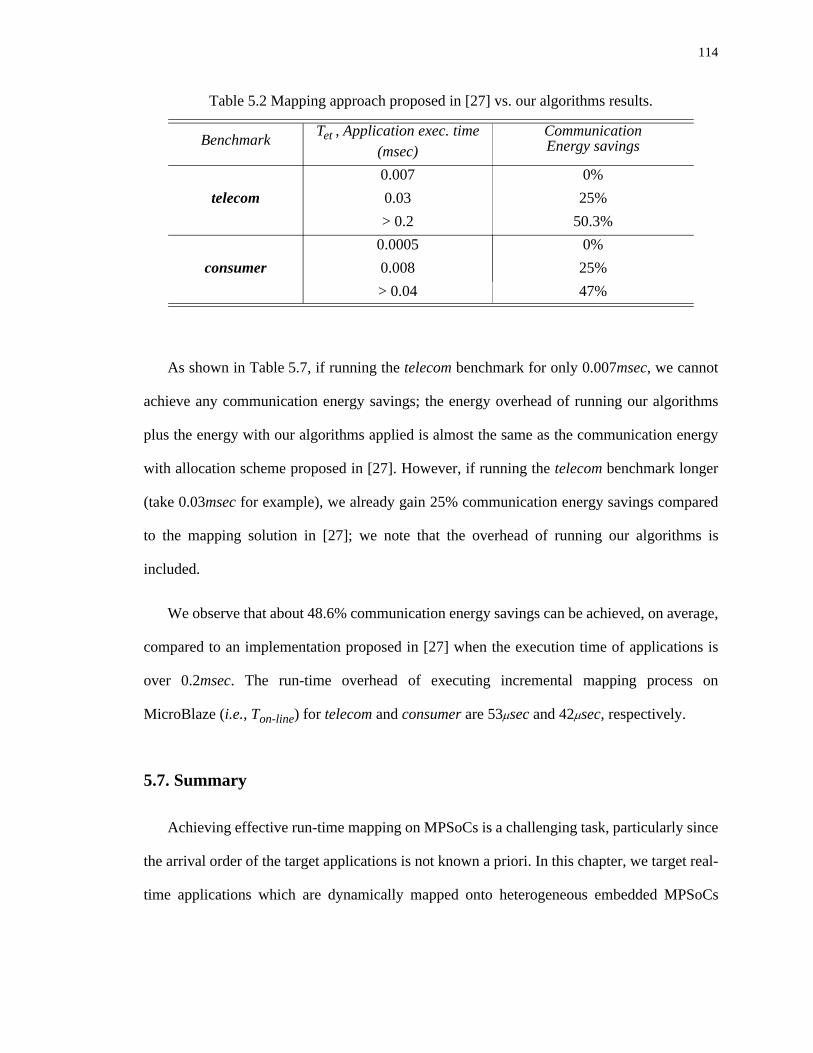
114

Table 5.2 Mapping approach proposed in [27] vs. our algorithms results.

As shown in Table 5.7, if running the telecom benchmark for only 0.007msec, we cannot

achieve any communication energy savings; the energy overhead of running our algorithms

plus the energy with our algorithms applied is almost the same as the communication energy

with allocation scheme proposed in [27]. However, if running the telecom benchmark longer

(take 0.03msec for example), we already gain 25% communication energy savings compared

to the mapping solution in [27]; we note that the overhead of running our algorithms is

included.

We observe that about 48.6% communication energy savings can be achieved, on average,

compared to an implementation proposed in [27] when the execution time of applications is

over 0.2msec. The run-time overhead of executing incremental mapping process on

MicroBlaze (i.e., Ton-line) for telecom and consumer are 53μsec and 42μsec, respectively.

5.7. Summary

Achieving effective run-time mapping on MPSoCs is a challenging task, particularly since

the arrival order of the target applications is not known a priori. In this chapter, we target real-

time applications which are dynamically mapped onto heterogeneous embedded MPSoCs

Benchmark Tet , Application exec. time (msec)

CommunicationEnergy savings

0.007 0%telecom 0.03 25%

> 0.2 50.3%0.0005 0%

consumer 0.008 25%> 0.04 47%

115

where communication happens via the NoC approach and resources connected to the NoC

have multiple voltage levels.

More precisely, we have addressed precisely the energy- and performance-aware

incremental mapping problem for NoCs with multiple voltage levels and proposed an efficient

technique (consisting of near convex region selection and vertex allocation processes) to solve

it. As shown, using the near convex region selection technique, the mapping results of our

algorithms can be obtained very efficiently; also, they are not far from the optimal case.

Moreover, additional incoming applications can be added into system with minimal

communication overhead. Experimental results have shown that the proposed technique is

very fast and as much as 50% communication energy savings can be achieved compared to

using an the state-of-the-art task allocation scheme.

Of note, in this chapter, we address the run-time resource management problem on the 2-D

mesh-based platform, i.e. platform with regular topology. However, the workload variation on

the system may result from the system itself or users’ interaction with the system; we further

discuss deeply about these two factors on run-time optimization in Chapter 6 and Chapter 7,

respectively.

117

6. FAULT-TOLERANT TECHNIQUES FOR ON-LINE

RESOURCE MANAGEMENT

6.1. Introduction

Resource utilization and system reliability are critical issues for the overall computing

capability of MPSoCs running a mix of small and large applications [23]. This is particularly

true for MPSoCs consisting of many cores that communicate via the NoC approach since any

failures propagating through the computation or communication infrastructure can degrade the

system performance, or even render the whole system useless. Such failures may result from

imperfect manufacturing, crosstalk, electromigration, alpha particle hits, or cosmic radiation,

and be permanent, transient, or intermittent in nature [145].

Existing fault-tolerant (FT) techniques for NoC resilience target the device, packet/data, or

end-to-end transaction levels of abstraction [53][142]. However, there is a need to

complement these approaches by handling failures at system-level and thus ensuring

resiliency while maintaining the required levels of system performance. From this perspective,

it has been shown that adding spare cores and wires can significantly improve the reliability,

reduce the cost, and be a substitute for the burn-in process [65][145]. For instance, for the

Intel 80-core processor [72], adding 10 or 20 spare cores to achieve 10 × 9 or 10 × 10

configurations, can make the system yield jump to 90% and 99%, respectively [146].

As shown in Figure 6.1, the NoC platform we consider is a 2-D tile-based architecture,

which consists of various resources and network elements. More precisely, the resources

consist of computational tiles (i.e. processors/cores/resources) and memory tiles, while the

118

network elements consist of routers, links, and resource-network interfaces. In the remaining

part of the chapter, we may use the term “resource” and the term “core” alternatively when

there is no ambiguity.

In terms of the computational tiles, we assume a j-out-of-i-core model [145]; that is,

except the distributed manager tiles that control the status of the entire system, the platform

consists of i cores where at least j of these i cores should be defect-free (or active, reachable)

cores responsible for running the application tasks in order to satisfy the system performance

requirements. In other words, if there exist k (permanent) faulty cores in the system due to the

imperfections in manufacturing (see the ‘flash sign’ in Figure 6.1), then we assign i-j-k cores

as spares for application computation. Of note, some design parameters given for the

model, i.e. i, j, and k, are related to the chip yield or manufacturing process; a more

detailed discussion on them can be found in [145][146].

Coming back to Figure 6.1, the main task of the manager titles (‘MA’ tiles in Figure 6.1)

is to 1) decide on resource management and 2) control the migration process via the platform

operating system. The role of a spare core (‘S’ in Figure 6.1) is to replace the (temporarily

Figure 6.1 Non-ideal 2-D mesh platform consists of resources connected via anetwork. The resources include computational tiles (i.e., manager titles, activeand spare cores) and memory titles. Permanent, transient, or intermittent faultsmay affect the computational and communication components on this platform.

: computational core/tile, type: ‘CP’

: router: links: distributed global MAnager

: Spare core: permanent faulty core: transient/intermittent faulty coreMEM MEM MEM

!

MA

MA

S

S

S!

MEM MEM MEM

!

MA

MA

S

S

S!

MA

MEM

S

!

: MEMory, type: ‘MEM’

119

or intermittent) faulty cores (see ‘!’ in Figure 6.1) or other unreachable cores (due to the

failure of the system interconnect). In other words, each active core has a probability p > 0 to

be affected by transient, intermittent, or permanent faults. We note that p is not a constant

during the chip lifetime, as it depends on chip lifetime cycles, processor utilization, or even

temperature. If necessary, the application tasks assigned to the active core will migrate to the

spares in order to continue being processed. Such task migration processes are controlled by

the distributed manager tiles.

Doing effective resource management for such irregular MPSoCs while failures occur

dynamically, and minimizing the communication energy consumption while maximizing the

entire system performance is a challenging task. It is obvious that the lack of regularity

increases the distance among various cores; this may further incur a higher network contention

on inter- or intra- application communication. In turn, the contention in the network may

degrade the system throughput. Critical factors for causing the system degradation need to be

quantified in order to handle the dynamic application mapping on such irregular platforms. In

addition, when a transient, intermittent, or permanent failure occurs, the system must be able

to isolate the failure from the offending resource and thus some mechanisms are needed in

order to avoid failure propagation to the rest of the system.

Given the above consideration, we address the problem of run-time fault tolerant resource

management, with the objective of allocating the application tasks to the available, reachable, and

defect-free resources in irregular NoC-based multiprocessor platforms (i.e., j-out-of-i computation

model with known and dynamic faulty probability p for each active core). The goal of this

dynamic technique is to minimize the communication energy consumption and network

contention, while maximizing the overall system performance. The challenge of the approach is

to manage the run-time and energy overhead for running such an algorithm, while maintaining

useful levels of fault tolerance in the network [42]. Our contributions are as follows:

120

• First, we explore the spare core placement problem and investigate the impact on failure

propagation probability.

• Second, we analyze the major factors that produce network contention before

investigating critical metrics for measuring the network contention and system

fragmentation, as well as their impacts on system performance.

• Third, we propose and evaluate an efficient algorithm for fault-tolerant resource

management with the goal of minimizing the communication energy consumption and

maximizing the overall system performance.

Taken together, these specific contributions improve the system-level resiliency, while

optimizing the communication energy consumption and the system performance.

The remaining of this chapter is organized as follows. In Section 6.2, we review the

relevant work. Section 6.3 analyzes the impact on network contention and spare core

placement. In Section 6.4, we investigate several critical metrics and provide insight into the

FT resource management problem on irregular platforms. The problem formulation and

details of the proposed FT algorithms are presented in Section 6.5. Experimental results are

presented in Section 6.6. Finally, we summarize our contribution in Section 6.7.

6.2. Related Work and Novel Contributions

There is a considerable work on online failures/errors diagnosis and detection for

multiprocessor systems at micro-architecture level with low power and area overhead

[49][96]. Besides this work, operating system control in NoC-based multiprocessor platforms

has been proposed to support system-level fault-tolerance [117]. Other techniques for failure/

error as well as thermal monitoring for NoC platforms have been proposed in [84][136]. More

recently, Huang et al. have taken the system lifetime reliability and system lifetime into

121

consideration at design time, while dealing with the application task mapping in NoC-based

MPSoCs [82]. In addition, transient failures on NoC links have also been considered under

stochastic and adaptive routing schemes [53][102][142].

There exists prior work on run-time application mapping on NoCs that aims at optimizing

the packet latency and power/energy consumption [27][79][110][154]. However, to the best of

our knowledge, this is the first work that considers the run-time fault-tolerant resource

management on non-ideal NoC platforms which is able to cope with the occurrence of static

and dynamic failures on both computational or communication components. Of note, while we

assume there exists a fault/error detection scheme with support for thermal monitoring, we

focus our attention on application mapping for such non-ideal NoC platforms which support

multiple applications entering and leaving the system dynamically.

6.3. Analysis for Network Contention and Spare Core Placement

6.3.1. Network Contention Impact

Since applications enter and leave the system dynamically, the application communication

contention is less likely to be avoided. Therefore, before proposing the mechanism for run-

time FT resource management (especially on such irregular NoC), it is definitely necessary to

figure out the impact of all possible communication contention on system performance; here,

we clarify them into three types: source-based, destination-based, and path-based contention.

Figure 6.2 captures one application mapping on mesh-based 3 × 3 NoC, where the application

characteristic is defined in Section 2.2.

• Source-based contention: it occurs when two traffic flows originating from the same

source contend for the same links, as shown in Figure 6.2(b).

122

• Destination-based contention: it occurs when two traffic flows which have the same

destination contend for the same links, as shown in Figure 6.2(c).

• Path-based contention: it occurs when two traffic flows which neither come from the

same source, nor go towards the same destination contend for the same links

somewhere in the network, as shown in Figure 6.2(d). These two traffic flows can be

from the same applications or from the different applications, so-called internal or

external network contention as defined in [98] and [99]. From the definition of path-

based contention, it mostly comes from the external contention.

To illustrate the impact of the source-based, destination-based, and path-based network

contention on the packet latency, we consider the following experiment, i.e., several mapping

configurations (see Figure 6.3) in a 4 × 4 mesh NoC: without/with only source-based

contention (cases 1 vs. 2), without/with only destination-based contention (cases 3 vs. 4), and

without/with only path-based contention (cases 5 vs. 6). We apply the XY routing and

wormhole switching for data transmission with 5 flits per packet. The communication rate (or

the packet injection rate from the source core) of transmissions in each configuration is set to

be the same. For fixed injection rates in each configuration, we run 100 different experiments

and calculate the corresponding average packet latency and throughput; the latency is

Figure 6.2 Application mapping on mesh-based 3 × 3 NoC (a) Application characteristicACG = (V, E) (b) Source-based contention (c) Destination-based contention (d) Path-based contention.

e12

e13 e13

e23 e24

e13

v1 v2 v3

v4

v1 v2 v3

v4

v1 v2 v3

v4

PEACG = (V , E)

e12

v4

v2

v1

v3

e13

e23e24

e43

(a) (b) (c) (d)

123

0.02 0.03 0.04 0.05 0.06 0.07 0.08 0.09 0.10

100

200

300

400

500case 1: without source-based contentioncase 2: with source-based contention

Figure 6.3 The (a) source-based (b) destination-based (c) path-based contention impacton average packet latency.

packet injection rate (packet/cycle)

avg.

pac

ket l

aten

cy

0.08 0.1 0.12 0.14 0.16 0.180

100

200

300

400case 3: without destination-based contentioncase 4: with destination-based contention


avg.

pac

ket l

aten

cy

0.1 0.15 0.2 0.25 0.3 0.35 0.40

100

200

300

400case 5: without path-based contentioncase 6: with path-based contention


avg.

pac

ket l

aten

cy

S DD

D

D

S D

D

D

D

case 1

case 2

(a)

D SS

SS

S

D S

S

S

S

case 3

case 4

(b)

D

D

D

S

S

SD

S

D

SD

D

D

S

S

S

case 5

case 6

(c)

124

calculated from the time when packets are generated from sources to the time when the

packets reach the destination. The results are plotted in Figure 6.3 with the x-axis showing the

total injection rate of all transmissions in that configuration and the y-axis showing the

average packet latency at the corresponding injection rate.

As seen in Figure 6.3(a), for source-based contention (i.e., cases 1 and 2), the throughput

is the same. This makes sense since every generated packet needs to pass through the link

from the source core to its router; therefore, the system performance is basically limited by the

injection rate of the source core.

For destination-based contention (i.e., cases 3 and 4 in Figure 6.3(b)), the system

throughput has about 2% improvement. We observe that the bottleneck of these two

configurations (i.e., cases 3 and 4) is actually due to the link between the router and its

corresponding destination core for which all packets contend. Obviously, such intra-tile

contention can be mitigated via careful hardware/software codesign (i.e., clustering process),

but can not be solved via mapping.

As seen in Figure 6.3(c), there is a dramatic throughput difference when comparing cases

5 and 6 (without/with path-based contention, respectively) as 118% throughput improvement

is observed (i.e., the throughput improves from 0.16 to 0.35 without path-based contention in

the network). Moreover, we observe that the frequency of occurrence of the path-based

contention is much higher compared to the source-based and destination-based contention as

the system size scales up. By doing several experiments involving many runs, we observed

that the ratio of path-based to source-based contention and the ratio of path-based to

destination-based contention increase linearly with the network size (i.e., for 4 × 4, 6 × 6,

8 × 8, and 10 × 10, the ratios are 1.2, 2.5, 4.0, 5.6, respectively). Therefore, in the remaining of

this chapter, we focus on minimizing the path-based contention since this has the most

significant impact on the packet latency and can be mitigated through the mapping process.

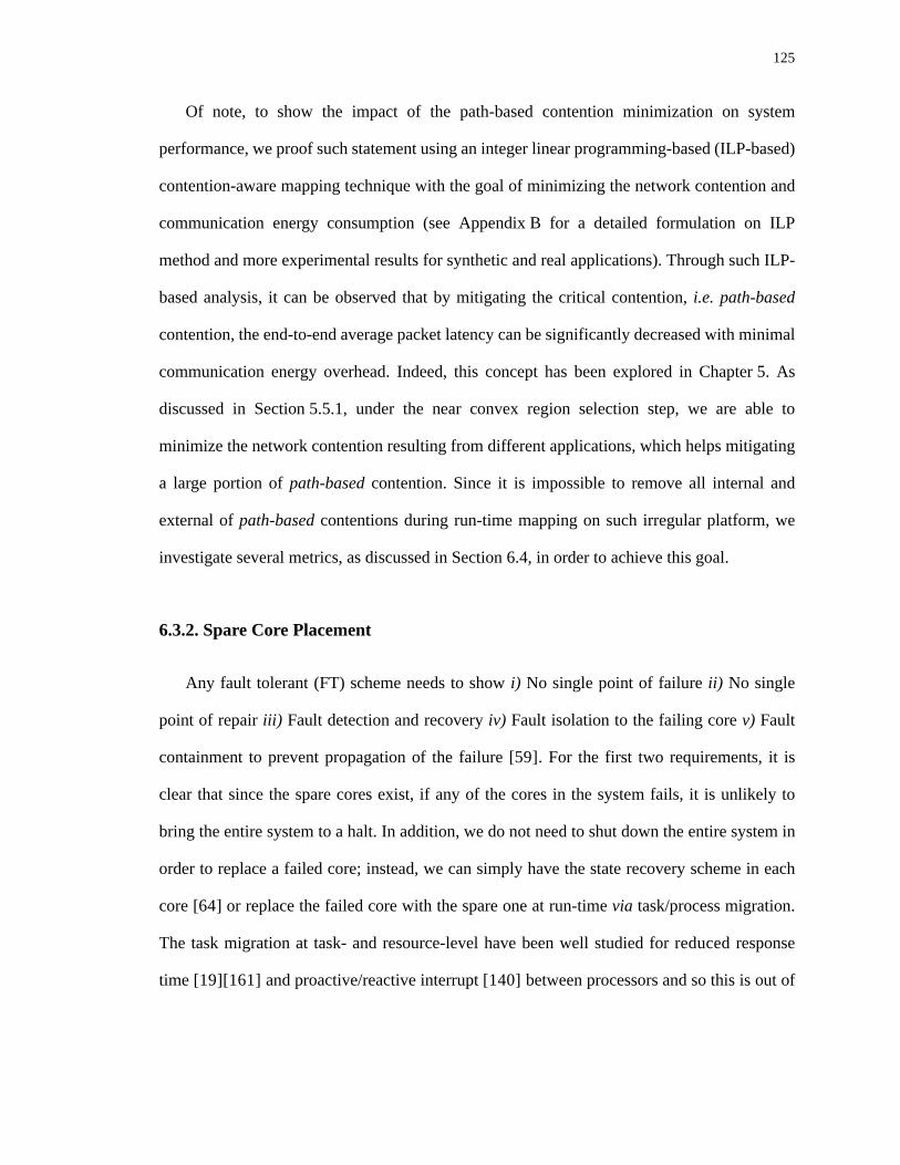
125

Of note, to show the impact of the path-based contention minimization on system

performance, we proof such statement using an integer linear programming-based (ILP-based)

contention-aware mapping technique with the goal of minimizing the network contention and

communication energy consumption (see Appendix B for a detailed formulation on ILP

method and more experimental results for synthetic and real applications). Through such ILP-

based analysis, it can be observed that by mitigating the critical contention, i.e. path-based

contention, the end-to-end average packet latency can be significantly decreased with minimal

communication energy overhead. Indeed, this concept has been explored in Chapter 5. As

discussed in Section 5.5.1, under the near convex region selection step, we are able to

minimize the network contention resulting from different applications, which helps mitigating

a large portion of path-based contention. Since it is impossible to remove all internal and

external of path-based contentions during run-time mapping on such irregular platform, we

investigate several metrics, as discussed in Section 6.4, in order to achieve this goal.

6.3.2. Spare Core Placement

Any fault tolerant (FT) scheme needs to show i) No single point of failure ii) No single

point of repair iii) Fault detection and recovery iv) Fault isolation to the failing core v) Fault

containment to prevent propagation of the failure [59]. For the first two requirements, it is

clear that since the spare cores exist, if any of the cores in the system fails, it is unlikely to

bring the entire system to a halt. In addition, we do not need to shut down the entire system in

order to replace a failed core; instead, we can simply have the state recovery scheme in each

core [64] or replace the failed core with the spare one at run-time via task/process migration.

The task migration at task- and resource-level have been well studied for reduced response

time [19][161] and proactive/reactive interrupt [140] between processors and so this is out of

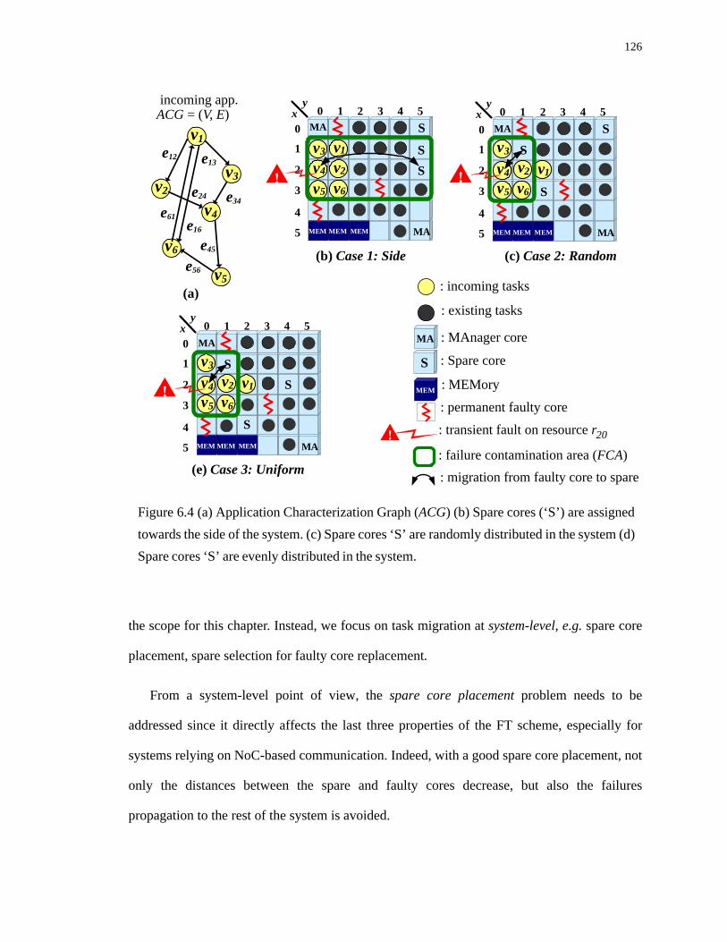
126

the scope for this chapter. Instead, we focus on task migration at system-level, e.g. spare core

placement, spare selection for faulty core replacement.

From a system-level point of view, the spare core placement problem needs to be

addressed since it directly affects the last three properties of the FT scheme, especially for

systems relying on NoC-based communication. Indeed, with a good spare core placement, not

only the distances between the spare and faulty cores decrease, but also the failures

propagation to the rest of the system is avoided.

e12

v3

v6

v4

v5

v2

e13

e34e24

e45

e56

e16

e61

v1

Figure 6.4 (a) Application Characterization Graph (ACG) (b) Spare cores (‘S’) are assignedtowards the side of the system. (c) Spare cores ‘S’ are randomly distributed in the system (d)Spare cores ‘S’ are evenly distributed in the system.

ACG = (V, E)

!

: existing tasks

: incoming tasks

: Spare core

: MAnager core

: permanent faulty core

: transient fault on resource r20

: failure contamination area (FCA): migration from faulty core to spare

(a)

(b) Case 1: Side (c) Case 2: Random

: MEMory

incoming app.

MA

S

MEM

0

1

2

3

4

S

S

v1

v3

v5

v2v4!

xy

v6

MA S

MEMMEM MAMEM5

0 1 2 3 4 50

1

2

3

4

0 1 2 3 4 5xy

v3

v5

v1

v4 v2! v6

MA S

SS

MEMMEM MAMEM5

0

1

2

3

4

S

S

v1

v3

v5

v2v4!

xy

v6

MA

S

MEMMEM MAMEM5

0 1 2 3 4 5

(e) Case 3: Uniform

127

Assume that an incoming application (see its ACG in Figure 6.4(a)) needs to be

mapped onto a 6 × 6 NoC platform interconnected via a mesh network under wormhole

switching and XY routing (if there exists failed links, use minimal-path routing instead).

Each resource rmn is located in the NoC at the intersection of mth row and nth column.

Several spare core placement schemes are studied here: Case 1) Side assignment: Assign

the spare cores to the side of the system (shown in Figure 6.4(b)), Case 2) Random

assignment: Randomly distribute the spare cores in the system (shown in Figure 6.4(c)),

and Case 3) Uniform assignment: Evenly distribute the spare cores in the system (shown

in Figure 6.4(d)), Case 3).

Intuitively, the distance among the active cores in Case 2 and Case 3 is higher than

that in Case 1 since the system size grows by involving the spares; this, in turn, results in

higher communication energy consumption and lower system performance. For example,

it can be seen that for the incoming application in Figure 6.4(b) and (c),

MD(e12) = MD(e13) = 1 in Case 1, while MD(e13) = 3 in Case 2. However, when a

transient fault occurs at core r20, the master will assign the closest spare to recover the

fault. Therefore, cores r25 and r11 are selected in these two cases which means that the

distance between the faulty core and the closest spare is 5 and 2, respectively. Moreover,

we define the failure contamination area (FCA) to reflect the failure propagation

probability, namely the greatest area resulting from the communication re-routing while

replacing the faulty core with a spare. As seen in Figure 6.4(a), since vertices v2, v3 and

v5 have the communication with vertex v4, the FCA in Case 1 is much higher than that in

Case 2. Shown as the thick frames in Figure 6.4(b), (c), and (d), the FCA value in Cases

1 and 2 is 18 and 6, respectively; this may further degrade the performance of some other

existing application shown with black dots in the system.

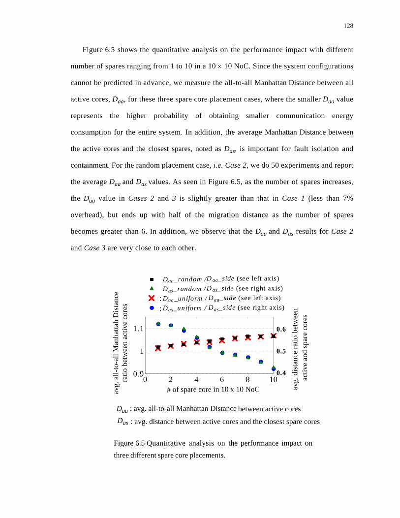
128

Figure 6.5 shows the quantitative analysis on the performance impact with different

number of spares ranging from 1 to 10 in a 10 × 10 NoC. Since the system configurations

cannot be predicted in advance, we measure the all-to-all Manhattan Distance between all

active cores, Daa, for these three spare core placement cases, where the smaller Daa value

represents the higher probability of obtaining smaller communication energy

consumption for the entire system. In addition, the average Manhattan Distance between

the active cores and the closest spares, noted as Das, is important for fault isolation and

containment. For the random placement case, i.e. Case 2, we do 50 experiments and report

the average Daa and Das values. As seen in Figure 6.5, as the number of spares increases,

the Daa value in Cases 2 and 3 is slightly greater than that in Case 1 (less than 7%

overhead), but ends up with half of the migration distance as the number of spares

becomes greater than 6. In addition, we observe that the Daa and Das results for Case 2

and Case 3 are very close to each other.

0.6

0.5

0.4

Daa_random / Daa_side (see left axis)Das_random / Das_side (see right axis)

0 2 4 6 8 100.9

1

1.1

::

0.6

0.5

0.4

Daa_uniform / Daa_side (see left axis)Das_uniform / Das_side (see right axis)

Daa_random / D aa_side (see left axis)Das_random / D as_side (see right axis)

Figure 6.5 Quantitative analysis on the performance impact onthree different spare core placements.

# of spare core in 10 x 10 NoC

Daa : avg. all-to-all Manhattan Distance

Das : avg. distance between active cores and the closest spare cores

avg.

all-

to-a

ll M

anha

ttah

Dis

tanc

e

ra

tio b

etw

een

activ

e co

res

avg.

dis

tanc

e ra

tio b

etw

een

activ

e an

d sp

are

core

s

between active cores

129

In conclusion, distributing spares at random or evenly within the system slightly

increases the all-to-all Manhattan Distance among the active cores. This may causes some

communication energy consumption during the mapping process, but it maintains useful

levels of fault isolation and containment compared to the scenario when spares are placed on

the sides. More evaluations on system throughput for spare core placement are shown in

Section 6.6.2.

6.4. Investigations Involving New Metrics

In practice, applications can enter and leave the system dynamically and since the faults

existing in the system can be transient or intermittent, the locations of faulty cores may

change at run-time. Therefore, our goal is to find a mapping function, map( ), for allocating

the incoming application tasks (see application modeling in Section 2.2) to the reachable,

available and fault-free cores on a non-ideal 2D mesh NoC platform (see Figure 6.1) such that

i) the communication energy consumption is minimized ii) the network contention is

minimized and iii) the entire system performance is maximized. Of note, the applications

execution time and their relative ordering are not known in advance, thus considering the entire

system optimization during mapping is the critical challenge for solving this problem. Again,

the application modeling and the communication energy modeling have been described in

Section 2.2 and Section 2.3, respectively. Even though we assume the platform under

consideration is based on a 2-D tile-based architecture and a wormhole switching scheme, we

emphasize that our proposed algorithms can be extended for other irregular topologies with

other switching schemes.

Three new performance metrics are defined next in order to reach these three goals of

finding the FT mapping function, map( ), as mentioned.

130

1. Weighted Manhattan Distance (WMD): Let vertices vi and vj be mapped onto resources

rab and rcd, respectively. The weighted Manhattan Distance between any two vertices is

defined by

comm(eij) × MD(map(vi) , map(vj)) = comm(eij) × (|a-c| + |b-d|) (6.1)

Based on the bit energy metric [170], it is obvious that the weighted Manhattan distance

is positively correlated with the communication energy consumption.

2. Link Contention Count (LCC): The link contention occurs when two communication

flows eij and ekl from the same or different ACGs, where i k and j l, contend for the

same link somewhere in the network. Such link contention can produce a significant

degradation on system performance.

3. System Fragmentation Factor (SFF): This factor reflects the degree to which the non-

contiguity of one application may affect other regions where vertices in different applications

may be allocated to. The system fragmentation factor is defined as

(6.2)

where w and h are the width and the height of the minimal enclosing rectangle covering

the mapping solution of ACG = (V, E), while f and s are the number of faulty cores and spares

in that rectangle, respectively. Therefore, the smaller SFF value for each application on the

system is a good indication of optimizing the entire system performance.

One example can be seen in Figure 6.6 where two possible mapping results (map( ) and

map’( )) are shown with solid and dotted circles, respectively. With the same ACG shown in

Figure 6.4(a), the WMD of vertex v1 and vertex v6 in map( ) is r(e16) × 2, while in map’( ) is

r(e16) × 5. Under the routing referring to Figure 6.6, the LCC in map( ) for the ACG is 1

(i.e. e13 and e24 share the same link,); the LCC in map’( ) is 5. In addition, the SFF in map( )

≠ ≠

SFF w h× V– f– s–w h×

-----------------------------------------=

131

for the ACG is 0.11 = 1/9 while that in map’( ) is 0.33 = 4/12. As seen, the larger the SFF, the

more interference exists between the cores from different applications (see the dashed line in

Figure 6.6(b)).

Now, we evaluate the composite effect of these three metrics (i.e., WMD, LCC, SFF) on

the average packet latency2. Several ACGs are generated using the TGFF package [162],

where the number of vertices ranges from 5 to 15. Then, we implement three different

scenarios (i.e., Random mapping (Random), Multiple Buddy Strategy (MBS) [99] and Nearest

Neighbor approach (NN) [27]) for allocating application tasks onto a 10 × 10 NoC with

randomly selected faulty and spare cores. For each scenario, the average packet latencies, as

well as the average values of the three metrics defined above are calculated for twenty

different system configurations.

We employ 3D Kiviat graphs to provide a composite view of the impact of these three

metrics [112]. A Kiviat graph consists of three dimensions, each representing one of the

aforementioned metrics emanating from a central point, as seen in Figure 6.7. Each metric

2. Of note, our objective function (i.e. system performance and communication energy consumption) ispositively correlated with the average packet latency [27][79].

Figure 6.6 Two mapping results for the ACG in Figure 6.4(a)where the spare cores are randomly placed on the platform.

(a) map( ) (b) map’( )

0

1

2

3

4

S

S

xMA S

MEMMEM MAMEM5

0 1 2 3 4 5

v6

v4

v5

v3v2v1

y

0

1

2

3

4

S

Sv1

v3

v5

v2v4

xy

v6

MA S

MEMMEM MAMEM5

0 1 2 3 4 5

132

varies from zero to the largest value observed in the experiments. As shown, the composite

view of three metrics lies within the shaded area. Intuitively, the smaller the area, the better

the system performance and the lower communication energy consumption corresponding to a

particular approach is.

Table 6.1 reports the values of these three metrics and the corresponding Kiviat area,

i.e. (K( )), while the system latency is measured in cycles and the communication energy

consumption is normalized to the Random approach. As we can see, due to its smaller

Kiviat area, the NN approach performs better and consumes lower communication energy

than the MBS and random approaches.

Table 6.1 Comparison among the Random, MBS [99], and Nearest Neighbor (NN) [27]

mapping methods.metrics \ mapping scenario Random MBS [99] NN [27]

WMD 0.95 0.60 0.2LCC 0.93 0.60 0.57SFF 0.94 0.85 0.58

Kiviat area 1.1478 0.5975 0.2427average packet latency 342.1 148.27 94.22

normalized comm. energy consumption 1 0.48 0.32

Figure 6.7 3D Kiviat plots showing WMD, LCC, and SFF metrics forthree difference mapping schemes (i.e., Random, MBS, and NN).

(a) Random (b) MBS (c) NN

WMD

LCC SFF

WMD

LCC SFF

WMD

LCC SFF

•

133

6.5. Fault-Tolerant Resource Management

In general, the FT resource management covers i) migrating tasks from faulty cores to

spares (discussed in Section 6.5.1) and ii) allocating the incoming application tasks to

available, reachable, and faulty-free cores (discussed in Section 6.5.2). The platform and

application models have been discussed in Section 2.1 and Section 2.2, respectively. Here,

we define some properties before formulating the FT scheme:

• There are two sets of cores/tiles rmn in the NoC platform, namely {CP, MEM} (see the

‘CP’ and ‘MEM’ cores in Figure 6.1)3.

• All applications have been done the off-line analysis and described by ACG = (V, E)

(see Section 2.2), where the type of each vertex vi, type(vi), can be either ‘t’ (i.e.,

representing a cluster of tasks) or ‘b’ (i.e., representing a buffer or memory unit). Tasks

belonging to the same cluster/vertex should run on their own defect-free computational

core (‘CP’), while the buffer module should be assigned to the memory tile ‘MEM’ of

the NoC platform.

• For rmn CP, s(rmn) stands for the status of core located at rmn. s(rmn) = -3 if the core

is assigned to be a spare, s(rmn) = -2 if the core is permanent faulty, s(rmn) = -1 if

the core is affected by transient or intermittent faults, s(rmn) = 0 if the core has

been already assigned to some application and s(rmn) = 1 if the core is idle/

available.

• map( ): vi map(vi) = rmn stands for a mapping function from one vertex to one

core.

3. As explained in Footnote 2 of Chapter 2, we may have memory module inside the MPSoC plat-form for memory intensive applications, as well as some vertices being characterized as a buf-fer unit in applications.

∈

→

134

The FT resource management strategy is described in Figure 6.8. Of note, in this chapter,

we assume that the failure rate of each core is updated based on the temperature of the core. In

addition, we apply the reactive task migration4 on faulty cores (see Section 6.5.1). As seen,

our scheme supports multiple applications entering and leaving the system dynamically (see

Section 6.5.2) and the distributed managers keep track of the cores status.

6.5.1. RUN_MIGRATION Process

Similarly to the control scheme in [117], our NoC platform includes the data and control

network. The reactive task migration procedure is given in Figure 6.9.

We note the FCA value in Step 02 (Figure 6.9) is highly dependent on the spare core

placement where its impact are evaluated in Section 6.3.2. The run-time and energy overhead

of Steps 1 and 3 are discussed in [19][161] based on the process response time and code

4. The reactive task migration process implies that after one core fails, it will be replaced by a spare,while the proactive task migration implies that the system manager monitors the failure probabilityof each core and migrates a failure-prone core to the spare before it actually fails. Although wefocus on the former scheme, it can be easily extended to become a proactive scheme with additionalNoC monitoring [84][117].

Figure 6.8 The FT resource management framework.

while(1){

if (faults are detected at rmn && migration is necessary)

RUN_MIGRATION(rmn);

if (one application ACGQ enters && resources are enough)

map(vi V in ACGQ) =RUN_FT_MAPPING(conf , ACGQ);

if (one application ACGP leaves) update rmn status where

rmn map-1(vi V in ACGP), s(rmn) 1;

}

∈

∀ ∈ ∈ →

135

sizes at task- and resource-level and is out of the scope of this work. Indeed, we consider

here task migration at system-level so we focus on spare core placement, spare selection for

faulty core replacement, etc. instead of showing the details of the task migration at task- and

resource-level (i.e., setup the interrupts in the codes for doing the migration, etc).

6.5.2. RUN_FT_MAPPING Process

Problem Formulation

Given the current system configuration, conf, and the incoming application ACGQ

Find map( ): vi map(vi) = rmn, vi V in ACGQ which minimizes the Kiviat area,

i.e. (K( )) corresponding to the three metrics, WMD, LCC, and SFF

Such that:

vi vj V, map(vi) map(vj) (6.3)

vi V and type(vi) = ‘t’, map(vi) = rmn CP and s(rmn) = 1 (6.4)

vi V and type(vi) = ‘b’, map(vi) = rmn MEM (6.5)

Figure 6.9 Main steps of RUN_MIGRATION process.

01: The failed core tmn sends out the message to themanager through the control network.

02: The distributed manager searches the closest availablespare which results in a smaller FCA value.

03: Execute the code migration or related data transmissionthrough the data network.

→ ∀ ∈

•

∀ ≠ ∈ ≠

∀ ∈ ∈

∀ ∈ ∈

136

Equation 6.3 means that each vertex should be mapped to exactly one tile and no tile can

host more than one vertex. Equation 6.4 and Equation 6.5 imply that the vertices should be

assigned to the correct type of resources in the system.

RUN_FT_MAPPING Algorithm

Any run-time algorithm must be lightweight and have a low energy consumption. Hence,

we define a few variables to achieve such a goal. For each tile t, the number of available (and

non-faulty) neighboring cores is stored in the variable neighbor[t], while the center of the

current resulting region R is stored in the variable center[R]. ED(tij , tkl) stands for the

Euclidean Distance between tiles tij and tkl, i.e. ED(tij , tkl) = (|i - k|2 + |j - l|2)1/2.

The steps of the RUN_FT_MAPPING algorithm are shown in Figure 6.10. We assume the

number of vertices of type ‘b’ and ‘t’ in the incoming ACG are S1 and S2, respectively.

In Steps 01-07, we select a region from the current system configuration with the goal of

minimizing the SFF; this helps reducing the LCC caused by different applications. Also the

number of cores belonging to the MEM and CP set should be equal to the number of vertices of

types ‘b’ and ‘t’ in ACG. Then, in Steps 08-10, we assign vertices to the selected region with

the goal of minimizing the WMD and LCC caused by this incoming application. With the

minimization of these three metrics, we seek to get a smaller Kiviat area through the

incremental mapping process.

The run time complexity of the FT algorithm is O(VlogV + ElogE). In Steps 03-07, if we

can search the possible tiles and store the information of neighbor[tmn] + ED(tmn, center[R])

of this wavefront in a HEAP, the complexity is O(VlogV). In Steps 08-10 with another HEAP

structure, it takes O(ElogE) to get the next un-assigned vertex from ACG and O(VlogV) to

find an available tile for it inside the region R. Of note, our FT approach can be implemented

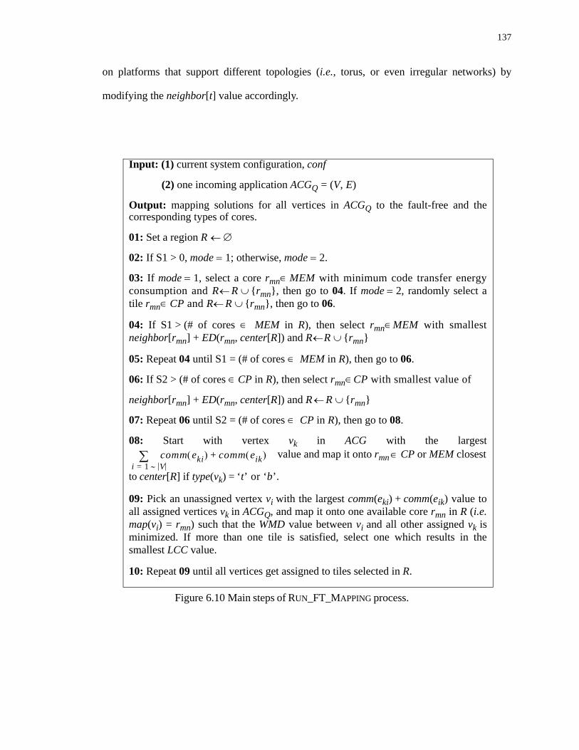
137

on platforms that support different topologies (i.e., torus, or even irregular networks) by

modifying the neighbor[t] value accordingly.

Figure 6.10 Main steps of RUN_FT_MAPPING process.

Input: (1) current system configuration, conf

(2) one incoming application ACGQ = (V, E)

Output: mapping solutions for all vertices in ACGQ to the fault-free and thecorresponding types of cores.

01: Set a region R

02: If S1 > 0, mode = 1; otherwise, mode = 2.

03: If mode = 1, select a core rmn MEM with minimum code transfer energyconsumption and R R {rmn}, then go to 04. If mode = 2, randomly select atile rmn CP and R R {rmn}, then go to 06.

04: If S1 > (# of cores MEM in R), then select rmn MEM with smallestneighbor[rmn] + ED(rmn, center[R]) and R R {rmn}

05: Repeat 04 until S1 = (# of cores MEM in R), then go to 06.

06: If S2 > (# of cores CP in R), then select rmn CP with smallest value of

neighbor[rmn] + ED(rmn, center[R]) and R R {rmn}

07: Repeat 06 until S2 = (# of cores CP in R), then go to 08.

08: Start with vertex vk in ACG with the largestvalue and map it onto rmn CP or MEM closest

to center[R] if type(vk) = ‘t’ or ‘b’.

09: Pick an unassigned vertex vi with the largest comm(eki) + comm(eik) value toall assigned vertices vk in ACGQ, and map it onto one available core rmn in R (i.e.map(vi) = rmn) such that the WMD value between vi and all other assigned vk isminimized. If more than one tile is satisfied, select one which results in thesmallest LCC value.

10: Repeat 09 until all vertices get assigned to tiles selected in R.

∅←

∈← ∪

∈ ← ∪

∈ ∈← ∪

∈

∈ ∈

← ∪

∈

comm eki( ) comm eik( )+i 1 V∼=

∑ ∈

138


6.6.1. Evaluation with Specific Patterns

In this section, we evaluate our FT mapping algorithm using a set of widely-used

workloads consisting of 1) communication-intensive applications with all vertices

communicating in an all-to-all fashion and 2) applications where all vertices communicate

with each other through a central memory only (denoted as one-to-all communication).

Several sets of applications are generated using the TGFF package [162] with the number of

vertices ranging from 5 to 35 in one ACG. The communication rates are randomly generated

according to some specified distributions. The sequences of incoming applications are also

generated randomly.

In terms of spare cores, we consider two spare core placement scenarios: 1) Side

placement, where all spares are assigned towards the sides and 2) Random placement, where

spares are randomly distributed across the platform. Also, 10% of the computational cores are

assumed to be permanently faulty due to the manufacturing process and randomly distributed

across the platform. As observed, the uniform spare core placement scenario (Case 3

discussed in Section 6.3.2) gives similar results to the random spare core placement; here we

report only the comparison between side and random placements.

To have a more accurate fault model, we use thermal modelling via HotSpot [73] to

estimate the temperature of each active computational core. We set the failure rate per cycle

for each core (at a room temperature of 25 C) to 10-9. Therefore, the estimated failure rate of

each core would be updated using the Arrhenius model [76] based on the temperature

obtained from the thermal measurements. In addition, in terms of the failure rate of the

memory, Alion System Reliability Analysis Centers report that the memory mean-time-

between-failure rates are around 700 years [74]. Also, since the on-chip buffer/memory

°

139

tiles benefit from built-in-self diagnostics and repair schemes, we assume that permanent

failures in memory do not occur at simulation.

Table 6.2 shows the throughput and communication energy consumption comparison

for two mapping approaches, namely 1) our proposed FT mapping (FT) and 2) Nearest

Neighbor (NN) [27]5, an heuristic which maps vertices with higher communication as closely

as possible, for NoCs of different sizes. All results are experimented from an NoC simulator

using C++ language.

As seen in Table 6.2 for the all-to-all communication, our proposed technique (FT)

achieves indeed a higher throughput and has a lower communication energy consumption

compared to the NN approach, especially for larger NoC platforms. Of note, our FT

approach works even better when the spares are located randomly in the platform

compared to the NN approach. For one-to-all communication, the system performance

cannot improve much since the bottleneck is mainly due to the memory module (i.e.,

accessing data to/from memory). Despite this, we still can achieve more communication

energy savings compared to the NN approach.

5. Even though the path load approach proposed in [27] performs the best, it does not consider any typeof failures in the cores of the platform so it is not directly comparable with our FT approach.

Table 6.2 Throughput and Energy Consumption between proposed FT and Nearest Neighbor (NN) approaches for all-to-all and one-to-all communication patterns.

space core placement-Side space core placement-Random

specific ACGs in different NoC size

throughput improvement (FT vs. NN)

comm. energy consumption

savings(FT vs. NN)

throughput improvement (FT vs. NN)

comm. energy consumption

savings(FT vs. NN)

5 × 5 all-to-all 23.2% 12.5% 23.5% 15.8%10 × 10 all-to-all 98.1% 32.1% 102.1% 36.2%30 × 30 all-to-all 163.2% 77.3% 178.2% 85.2%5 × 5 one-to-all 3.4% 13.8% 4.1% 17.8%

10 × 10 one-to-all 5.7% 17.5% 6.9% 23.6%30 × 30 one-to-all 19.4% 32.8% 25.9% 54.1%

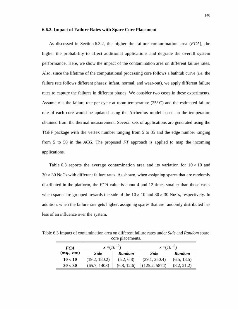
140

6.6.2. Impact of Failure Rates with Spare Core Placement

As discussed in Section 6.3.2, the higher the failure contamination area (FCA), the

higher the probability to affect additional applications and degrade the overall system

performance. Here, we show the impact of the contamination area on different failure rates.

Also, since the lifetime of the computational processing core follows a bathtub curve (i.e. the

failure rate follows different phases: infant, normal, and wear-out), we apply different failure

rates to capture the failures in different phases. We consider two cases in these experiments.

Assume x is the failure rate per cycle at room temperature (25 C) and the estimated failure

rate of each core would be updated using the Arrhenius model based on the temperature

obtained from the thermal measurement. Several sets of applications are generated using the

TGFF package with the vertex number ranging from 5 to 35 and the edge number ranging

from 5 to 50 in the ACG. The proposed FT approach is applied to map the incoming

applications.

Table 6.3 reports the average contamination area and its variation for 10 × 10 and

30 × 30 NoCs with different failure rates. As shown, when assigning spares that are randomly

distributed in the platform, the FCA value is about 4 and 12 times smaller than those cases

when spares are grouped towards the side of the 10 × 10 and 30 × 30 NoCs, respectively. In

addition, when the failure rate gets higher, assigning spares that are randomly distributed has

less of an influence over the system.

Table 6.3 Impact of contamination area on different failure rates under Side and Random spare core placements.

FCA (avg., var.)

x =(10 -9) x =(10 -6)Side Random Side Random

10 × 10 (19.2, 180.2) (5.2, 6.8) (29.1, 250.4) (6.5, 13.5)30 × 30 (65.7, 1403) (6.8, 12.6) (125.2, 5874) (8.2, 21.2)

°

141

6.6.3. Evaluation with Real Applications

We evaluate the potential of our algorithm on several real applications, namely five

benchmarks from the Embedded System Synthesis Benchmarks Suite [50], a video object

plane decoder, the MPEG4 decoder, picture-in-picture, and multi-window display

applications, where the last four applications include several memory modules. The

ACGs of these nine applications are built through an off-line analysis; applications are

randomly selected to enter and leave the system.

The Nearest Neighbor (NN) mapping approach in [27] is evaluated against our FT

method. Also, the comparison of 1) the average packet latency (i.e., the time elapsed between

packet generation at the source core and packet arrival at the destination core, in cycles), 2)

communication energy consumption, and 3) the Kiviat area, on these approaches are given in

Table 6.4. In each run, 5%-15% of the computational cores are assumed to be

permanently faulty and randomly distributed in the system. We report the average results

of running 50 runs for each mapping approach under different NoC sizes (e.g. 10 × 10

NN). We note that the range of each metric in the Kiviat graph is normalized from zero to the

largest value observed in random mapping implementation. The same fault model is applied

as that in Section 6.6.1. In addition, the overhead of the energy consumption for running

our FT algorithm is included in the communication energy consumption measurement.

As shown in Table 6.4, our approach can obtain lower average packet latency and smaller

communication energy consumption compared to the NN approach. The data of the Kiviat

area also imply that by minimizing the WMD, LCC, SFF metrics, we are able to reduce the

average packet latency quite significantly; this, in turn, increases the system performance and

decreases the communication energy consumption. The run-time overhead for running the FT

(see Figure 6.10) and NN approaches on a 100MHz MicroBlaze processor acting as a

142

distributed manager is, on average, 68μs and 46μs, respectively; these values are well suited

to this kind of on-line optimizations.

6.7. Summary

In this chapter, we have proposed a system-level fault-tolerant approach addressing the

problem of run-time resource management in non-ideal multiprocessor platforms where

communication happens via the NoC approach. The proposed application mapping techniques

in this new framework aim at optimizing the entire system performance and communication

energy consumption, while considering the static and dynamic occurrence of permanent,

transient, and intermittent failures in the system. As the main theoretical contribution, we have

analyzed the main factor of producing network contention and addressed the spare core

placement problem with its impact on system fault-tolerant (FT) properties. Then we have

investigated several critical metrics and provided insight into the resource management

process. Finally, a FT application mapping approach for non-ideal multiprocessor platforms

has been presented. Experimental results have shown that our proposed approach is efficient

and highly scalable; significant throughput improvements can be achieved compared to the

existing solutions that do not consider possible failures in the system.

Table 6.4 Comparison between the Nearest Neighbor (NN) and our FT mapping results on the overall system performance.

NoC size mapping approach avg. latency

normalized comm. energy consumption

Kiviat area

10 × 10NN [27] 105.37 1 0.264

FT 63.82 0.54 0.051

20 × 20NN [27] 191.28 1 0.351

FT 67.33 0.37 0.042

30 × 30NN [27] 275.12 1 0.383

FT 66.33 0.29 0.021

143

7. USER-AWARE DYNAMIC TASK ALLOCATION

7.1. Introduction

As discussed in Figure 1.3, for multiple use-case NoCs (such as Tile64TM by Tilera

[164] which deliver high performance computing for embedded applications), different

system configurations resulting from unpredictable failures (presented in Chapter 6) or

multi-user behaviors are too dynamic and too complex in nature to be modeled off-line.

As discussed about the user-centric design flow (see Figure 1.8), even though after having

generated NoC platforms which exhibit less variation among the users’ behavior (see

Chapter 4), there still exists some variation between the targeted platform and users within

each cluster (see the distance between the squares and the dots belonging to that cluster in

Figure 1.1). Therefore, the need for more sophisticated light-weight run-time optimization

for maximizing the user satisfaction and adapting to different user needs becomes

apparent (see the arrows in Figure 1.1). This chapter focuses on the resource management

problem, more precisely, task allocation problem while taking the user behavior into

consideration1.

The task allocation problem has been a key issue for performance optimization in parallel

and distributed systems [10][15][16][29][95][98][99][165]. To date, contiguous (see

Figure 7.1(a)) and non-contiguous (Figure 7.1(b)-(e)) allocation techniques have been

1. Our user-centric run-time optimization proposed in this chapter can also be applied to the non-idealplatform, i.e. platform with permanent, transient, or intermittent faults discussed in Chapter 6.

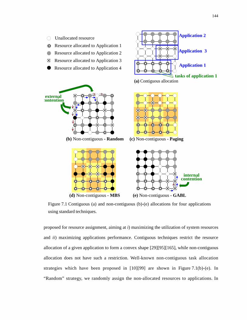
144

proposed for resource assignment, aiming at i) maximizing the utilization of system resources

and ii) maximizing applications performance. Contiguous techniques restrict the resource

allocation of a given application to form a convex shape [29][95][165], while non-contiguous

allocation does not have such a restriction. Well-known non-contiguous task allocation

strategies which have been proposed in [10][99] are shown in Figure 7.1(b)-(e). In

“Random” strategy, we randomly assign the non-allocated resources to applications. In

Unallocated resourceResource allocated to Application 1Resource allocated to Application 2Resource allocated to Application 3

external contention

Application 1

tasks of application 1

internal contention

Resource allocated to Application 4

Application 2

Application 3

Figure 7.1 Contiguous (a) and non-contiguous (b)-(e) allocations for four applicationsusing standard techniques.

(b) Non-contiguous - Random (c) Non-contiguous - Paging

(d) Non-contiguous - MBS (e) Non-contiguous - GABL

(a) Contiguous allocation

145

“Paging” and “Multiple Buddy Strategy (MBS)”, the mesh network is divided into non-

overlapping sub-meshes initially. “Paging” selects the non-allocated sub-meshes in row-

major order, while “MBS” allocates applications to contiguous sub-meshes if possible.

“Greedy-Available-Busy-List (GABL)” allocates resources from the largest free sub-

mesh of any size. The contiguous strategy achieves only 34% to 66% resource utilization

[95], while the latter can reach up to 78% [165]. However, the performance of non-contiguous

allocation may suffer due to internal and external contention caused by messages originating

from the “same” or “different” applications, respectively, contending for the same link. Of

note, there is no external contention for contiguous allocation (see Figure 7.1(a)) because the

tasks of the same application belong to a convex region, while tasks from different

applications do not communicate among them (also, application tasks are not reallocated

once they start executing).

The resource management techniques proposed so far for SoCs rely on a resource

manager operating under the control of an operating system (OS) [117]; this allows the

system operate effectively in a dynamic manner. Since SoC design is moving towards a

communication-centric paradigm [17], new metrics (e.g., physical links with limited

bandwidth, communication-energy minimization) need to be considered in the resource

management process. Indeed, with inadequate task assignment, the system will likely perform

poorly. As an example, the “Random” case in Figure 7.1(b) causes severe internal/external

network contention; this contention incurs a longer transmission latency and smaller system

throughput.

This chapter focuses on proposing an effective run-time resource management onto

embedded NoC-based MPSoC. Given that the arrival order and the execution time of the

target applications is not known a priori, achieving effective run-time resource management

on such platform is a challenging task. Of note, as discussed in Figure 6.3.1, the path-based

146

internal and external contention especially have large impact on system performance.

Compared to Chapter 5, Chapter 6, and the previous work, our contributions in this chapter

are as follows:

• Propose strategies for minimizing the path-based internal and external network

contention.

• Present algorithms for resource management while incorporating certain user

characteristics to better respond to run-time changes.

• Propose light-weight machine learning techniques for learning structures with critical

parameters/thresholds which are able to adapt to different types of users.

Different users result in different system configurations which cannot be predicted and

modeled at design time. Consequently, how to react to run-time stimuli the system receives,

while maintaining high performance is our main objective in this chapter. The best known

example for considering external interactions (e.g., human users) to the electronic devices is

perhaps the e-commerce site “Amazon.com”. An interface collecting various data on user

activity (e.g., who is interested in what and when) helps the search engine recommend users

what products to buy. Also, the context-aware mobile computing utilizes wearable sensor

devices for sensing the users and their current state to exploit the context information and

reduce the demand for human attention [77].

We believe that our approach aimed at incorporating the user behavior in resource

management can automatically adapt to different user needs. In other words, the technique is

well-suited to be embedded in future products belonging to the second and third categories in

Table 1.1.

This chapter is organized as follows: In Section 7.2, we review related work. The system

description and our newly proposed methodology are described in Section 7.3. The run-time

147

task allocation problem is formulated in Section 7.4 and efficient algorithms to solve it are

presented in Section 7.5. The on-line light-weight user model learning process is explained in

Section 7.6. Experimental results in Section 7.7 show the kind of communication energy

savings that can be achieved by considering the user behavior. Finally, we summarize our

contribution in Section 7.8.

7.2. Related Work

The resource management problem has been addressed in the literature in various contexts

like supercomputers, parallel and distributed systems, SoCs, etc. While having the goal of

maximizing the system performance, many techniques such as partitioning, mapping,

scheduling, resource sharing, load balancing have been proposed to date. Pastrnak et al.

present methods such that several tasks can run concurrently by exploiting the task- and data-

level parallelism [127]. Chang et al. address the coarse-grain task partitioning and clustering

problem to preserve the modularity of the initial application description [29]. Moreira et al.

propose an online resource allocation heuristic for multiprocessor SoCs which can achieve

utilization values up to 95% [111]. Nollet et al. apply task migration to improve the system

performance by reconfiguring the hardware tiles [118] and propose the adaptive routing to

ensure the quality-of-service requests of various applications [117]. Smit et al. propose a run-

time task assignment algorithm on heterogeneous processors [154] targeting on the current

system configuration.

Some prior work does consider the whole system configuration. For instance, Murali et al.

propose an off-line methodology for mapping multiple use-cases (with different

communication requirements and traffic patterns) onto NoCs [105]. Also, Pop et al. present

the incremental design approach of distributed systems for hard real-time applications over a

bus [130].

148

With the ever-increasing connectivity between systems and users, how to design an

electronic system which can examine and mediate people’s interactions is becoming an

important challenge. We first addressed the run-time task allocation problem on NoC-based

platforms, while considering the user behavior in [36]. Then, we generalize the technique in

[36] to include the user behavior and pre-defined user model in the energy optimization

process and then propose a light-weight machine learning technique for boosting the user

model at run-time. We show that by taking the user behavior into consideration during the

task allocation process and building a specific model for each user, the system can respond

much better to run-time changes and adapt dynamically to user needs.

7.3. Preliminaries and Methodology Overview

7.3.1. Motivational Examples

Our motivational example of run-time task allocation with user behavior taken into

consideration is given in Figure 7.2. When an event occurs (e.g., an application enters the

system), our objective is to allocate the tasks belonging to this application to the available

resources on the platform such that the path-based internal/external network contention

and communication cost can be minimized. In the remaining part of this chapter, the term

“internal/external contention” stands for path-based internal/external contention where it

occurs when two traffic flows which neither come from the same source, nor go towards the

same destination contend for the same links somewhere in the network (see definition in

Section 6.3.1). More precisely, reducing the internal contention always comes with the

benefit of minimizing the communication cost; however, this increases the probability of

external contention for additional mappings. More details can be found in the example

discussed in Figure 7.2. Figure 7.2(a) describes the characteristics of applications App 1 -

149

at time 4

Time

0 1 2 3 4

1

11

23

45

67

8

4 567 8

1213

1014

9

111213

10149

18161915

20 17

1816

17

1915

20

18 16171915

20

2122

2324

25

2122

232425

2122

232425

App 11

App 2 App 3 App 4 [0, App 1, 5][1, App 2, 6][2, App 3, 12][3, App 4, 13][4, App 5, 9]2 3

45

6 78

9

11

10 12

13 14

1516 17

18 19 2021

22 23

24 25

App 5

2 2

2

10 101010

1

1 1 1

1 2 2

2 2 25 5

5 5

at time 0 at time 1 at time 2 at time 3

12

3

12

3

12

3

12

3

12

3

12

3

12

3

12

3

12

3

12

3

12

3

12

3

12

3

12

3

45

67

8 45

67

8 45

67

8

45

67

8 45

67

8 45

67

8 45

67

8

111213

1014

9

111213

1014

91816

17

1915

20

4 567 8

4 567 8

4 567 8

111213

10149

111213

10149

111213

10149

111213

10149

111213

10149

18 16171915

20

18161915

2017

Approach 1: primarily minimize internal metrics

Approach 2: primarily minimize external metrics

Hybrid approach: user behavior considered

Figure 7.2 Motivational example of run-time resource management with user behaviortaken into consideration. (a) Application characteristics. (b) Events in the system. (c)(d)(e)Task allocation scheme under Approach 1, Approach 2, and Hybrid approach, respectively.

(a) Application characteristics (b) Events

(c)

(d)

(e)

150

App 5. More precisely, each vertex vi contains a cluster of tasks that will acquire a resource

later. Each edge eij represents the communication between two vertices vi and vj, while the

weight of each edge, r(eij), gives the corresponding communication rate (e.g., bits/sec).

Figure 7.2(b) shows the events in the system; one event [t1, Q, t2] represents App Q running

in the system from time t1 (sec) to t2 (sec) as defined in Section 2.3.1. Figure 7.2(c), (d), and

(e) show the system configurations at particular times 0, 1, 2, 3, and 4 under three different

approaches. At each specific time, a new application arrives in the system and creates a more

complex configuration. These three different approaches are as follows:

• Approach 1: Focus primarily on minimizing the internal contention and communication

cost; minimize the external contention only as a secondary goal.

• Approach 2: Focus primarily on minimizing the external contention; minimize the

internal contention and communication cost only as a secondary goal.

• Hybrid approach: A hybrid method consists of combining Approaches 1 and 2 with user

behavior taken into consideration.

As observed in Figure 7.2(c), when the system utilization increases, in Approach 1, the

remaining (available) resources are quite dispersed; this results in an increase of external

contention and incurs a higher communication overhead for additional mappings. On the

contrary, in Approach 2 (see Figure 7.2(d)), the regions occupied by applications (shown with

thicker lines) are near convex; this helps reducing the external contention and lessen the

additional communication costs. For example, as shown in Figure 7.2(d) at time 1, there is no

external contention under such configuration. However, the drawback of Approach 2 is that

with this near convex region limitation, we can only obtain the sub-optimal communication

cost for the incoming application. It is hard to judge which approach is an adequate solution to

the run-time task allocation problem, particularly when the application characteristics are not

151

known a priori. Therefore, in this chapter, we address this very issue and present a hybrid

allocation approach leveraging Approaches 1 and 2 while considering the user interaction with

the system.

Here, we consider at least one PE acting as a global manager which observes the user’s

behavior for a long session (or episode). Also, with the same example shown in Figure 7.2,

we assume that the manager predicts that applications App 2 and App 4 have a higher

probability to become critical applications since the former application has a higher

communication rate, while the latter one has a long presence in the system according to the

user’s behavior traces. In the hybrid approach, Approach 1 is applied only to the critical

applications.

In this example, we assume that the minimal-path routing is used to transmit data. For

simplicity, the communication cost (i.e. energy consumption in bits, EQ) of the event

[t1, Q, t2] is defined as follows:

(7.1)

where MD(vi , vj) represents the Manhattan Distance between any two vertices, vi and vj,

connected to each other in App Q. The event communication cost for each application under

different approaches is summarized in Table 7.1.

Table 7.1 Event communication cost [in bits] for three approaches and five applications entering in the system as shown in Figure 7.2.

App 1 App 2 App 3 App 4 App 5Approach 1 40 200 50 100 175Approach 2 40 250 60 120 125

Hybrid approach 40 200 60 100 125

EQ MD vi vj,( ) comm eij( )×( ) t2 t1–×i j,( ) in App Q∀

∑=

152

As shown in Figure 7.2(c), the internal contention is indeed minimized for the first four

applications and these four events consume the least amount of communication cost by time 3

(see Table 7.1 under Approach 1). However, the remaining (available) resources are quite

dispersed (see (Figure 7.2(c) at time 3)) when the system utilization increases; this results in

an increase of external contention and therefore it will incur a higher communication overhead

for any additional mapping. As shown in Table 7.1, the event communication cost for App 5

under Approach 1 is about 40% higher than those under Approach 2 and the hybrid approach.

On the contrary, in Approach 2, the regions occupied by applications (shown with thicker

lines) are near convex; this helps reducing the external contention and decreasing the

additional communication costs (compare Figure 7.2(c) and (d) at time 3). However, the

drawback of Approach 2 is that with this near convex region limitation, we can only obtain the

sub-optimal communication cost for the incoming application. In other words, it does not

work well when the system utilization is low (see Table 7.1 and compare the cost of App 2, 3,

and 4 of Approach 2 with that of Approach 1). For Approaches 1 and 2, it is hard to judge

which one is the adequate solution to the run-time task allocation problem, particularly when

the application characteristics are not known a priori.

Our motivation for applying the hybrid approach is to leverage the advantages offered by

both approaches 1 and 2; that is, we aim at balancing the internal/external contention and,

subsequently minimize the event communication cost (see Table 7.1). The basic idea is that,

by observing the user’s behavior, we can predict what the critical applications are and then

minimize their communication cost via Approach 1. Even if this may cause a larger external

contention, this can be later mitigated by applying Approach 2 to other applications.

Moreover, we observe that mitigating the internal and external contention reduces the

system fragmentation, which has a huge impact on system throughput. To show the influence

of system fragmentation on the mapping quality, we consider two scenarios for multiple

153

application mappings on 6 × 6 and 10 × 10 mesh NoCs, respectively, while considering fifteen

to twenty five vertices having all-to-all communication in each application: Scenario 1)

randomly and contiguously select the unused resources for each application Scenario 2) apply

either Approach 1 or Approach 2. We observe that the system throughput in the second

scenario improves by 45% and 108% compared to the first scenario, which implies that

mitigating the internal and external contention not only helps minimizing the communication

overhead for additional mappings, but also has a huge impact on maximum system

throughput.

Of note, the reallocation of resources to defragment the system, also called task migration,

is a complementary approach aimed at achieving load balancing and high resource utilization.

For distributed systems without shared memory support, the task migration policy must be

implemented by passing messages among resources; the implicit migration cost is large due to

the need of moving the process context [161]. Therefore, in this chapter, we do not consider

the task migration process. Instead, we target an run-time mapping process which does not

need to change the current system configuration.

7.3.2. System Description

As mentioned in Chapter 2, our embedded NoC platform is based on a 2-D mesh

architecture consisting of heterogeneous processing resources (i.e., master PEs running

the OS acting as global managers and several slave processor/PEs as shown in

Figure 2.1(a)). Each segmented link li between PEs has the same bandwidth B(li). We

further assume that each slave processor SPi has its computation capability, CC(SPi), with

level set from 1 to i. In addition, the slave processors in our system are processor-based

cores, e.g. Digital Signal Processor (DSP), ARM, and all application codes are compiled

already and stored in the global program memory where each slave process can easily access.

154

In the remaining part of the chapter, we may use the term “master PE” and “global manager

(GM)” alternatively when there is no ambiguity.

The real-time OS built in our embedded system is designed to be very compact and

efficient, such as Open AT OS provided by Wavecom [77]. We assume such OS supports non-

preemptive multi-tasking and event-based programming. More precisely, the OS control

mechanism as presented in Chapter 2 can be used to provide predictable and controllable

resource management, which includes monitoring the user’s behavior and making the task

allocation/mapping decision only when new events occur.

The communication infrastructure in such platform consists of a Data Network and a

Control Network (shown as solid and dotted lines, respectively, in Figure 2.1) which supports

minimal-path routing scheme2 and worm-hole switching. And the sum of all communication

flows passing through the link li cannot exceed its bandwidth B(li). Under such a platform,

the bit energy model as presented in Section 2.3.3 can be used to derive the communication

energy consumption of the entire system analytically. Assume now that applications enter

and leave the system at time t, where t is an integer. The total communication energy

consumed by some events in any session/episode si under a certain user model ST, during time

interval t = 0 ~ , is denoted by:

(7.2)

where is the length of session si and where stands for the communication

energy consumption of any application Q per time unit (see Section 2.3.3).

2. After the mapping of the incoming application is done, elimination of possible deadlocks betweenthe communication traces can be achieved by adding additional virtual channels in the router as apost-processing step [46]. In this chapter, we focus on the mapping step.

Tsi

Ecomm TsiST,( ) Ecomm

App Q ΔApp Q t( )t 1=

Tα

∑⎝ ⎠⎜ ⎟⎜ ⎟⎛ ⎞

×all applications

∑t 1=

Tsi∑=

TsiEcomm

App Q

155

7.3.3. Overview of the proposed methodology

We assume that all applications have been characterized by the Application Characteristic

Graph ACG = (V, E) as presented in Section 2.2. Our proposed methodology handling the

user-aware task allocation includes three stages as shown in Figure 7.3. In stage 1, when a

user starts first signing in the system, the master PE uses the default approach (i.e., Approach

2) for application mapping and, at the same time, records the user sequences that characterize

Figure 7.3 Overview of the proposed methodology. Default approach (i.e., Approach 2) isapplied in stage 1. Hybrid approach with pre-defined user model is applied in stage 2. Hybridapproach with on-line learned user model is applied in stage 3.

Done by Master Processor

Application Characteristics

EventTrigger

Approach 2

System Configuration


Pre-defined User Model

System Configuration


On-line Learned User Model

Minimize external

contention

Approach 2Minimize external

contention

Approach 1Minimize internal

contention

user sequences

user

sequ

ence

s

user

sequ

ence

s

user

sequ

ence

s

user

sequ

ence

s

user sequences

user sequences

user sequences

stage 1

EventTrigger

stage 2

Approach 2Minimize external

contention

Approach 1Minimize internal

contention

EventTrigger

stage 3

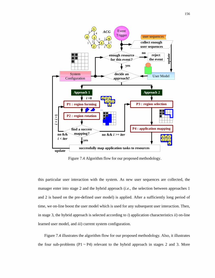
156

this particular user interaction with the system. As new user sequences are collected, the

manager enter into stage 2 and the hybrid approach (i.e., the selection between approaches 1

and 2 is based on the pre-defined user model) is applied. After a sufficiently long period of

time, we on-line boost the user model which is used for any subsequent user interaction. Then,

in stage 3, the hybrid approach is selected according to i) application characteristics ii) on-line

learned user model, and iii) current system configuration.

Figure 7.4 illustrates the algorithm flow for our proposed methodology. Also, it illustrates

the four sub-problems (P1 ~ P4) relevant to the hybrid approach in stages 2 and 3. More

Figure 7.4 Algorithm flow for our proposed methodology.

no

yes

upda

te

User ModelSystem Configuration

decide an approach?

user sequences

i =0

P1 : region forming

P2 : region rotation

Approach 1

find a success mapping?

yesno && i < iter

i = i

+1

P3 : region selection

P4 : application mapping

Approach 252 7

136

4

...

63

5 72

41

no && i >= iter

successfully map application tasks to resourcesupdate

ACG1

23

64

7

5

2

4

5

3

1

2

211

enough resource for this event?

reject the event

collect enough user sequences

EventTrigger

157

precisely, for Approach 1, we first form a region to minimize the internal contention for the

incoming application (P1) and then rotate/translate the resulting region to fit the current

system configuration (P2). For Approach 2, in order to minimize the external contention, we

do the opposite, namely first select a near convex region based on the current configuration

(P3), and then map the application tasks onto the selected region (P4). The detailed

explanation and objective of each subproblem are explained in Section 7.4.

Note that if the number of vertices in an application is greater than the total number of

available resources, the system can, in principle, reject this application or start it at a different

level of granularity (which may result in lower performance). Since we focus on task

allocation, we use the first mechanism; changing the application granularity at run-time is left

for future work.

7.3.4. User Modeling

As shown in Figure 7.3 (i.e., steps from stage 2 to stage 3), the manager records many user

sequences for a specific user and then, at run-time, it builds the user model which is able to

predict the probability of a certain application as being critical. Considering the run-time

overhead, we propose two ratios for building this model.

• Instantaneous communication rate ratio ( ): the ratio between the communication

rate of application Q (bits per time unit) and that of all applications occurring from

time 0 to T.

(7.3)

• Cumulative communication energy ratio ( ): Ratio between the communication energy

consumption of application Q active in the system ( (t) = 1 if Q is active between times

α

α

r eij( )eij∀ E in AppQ∈

∑

r eij( )eij∀ E in AppQ∈

∑⎝ ⎠⎜ ⎟⎛ ⎞

AppQ ever occured∀∑

---------------------------------------------------------------------------------------------------=

β

Δ

158

t-1 and t, and 0 otherwise) and the communication energy of all events in the system from

time 0 to T.

(7.4)

Later on, we introduce an user model based on two threshold/parameters, and , for

the master PE predicting whether the incoming application is critical or not for a particular

user. As mentioned, if the incoming application is recognized as critical, then Approach 1 is

applied; otherwise, Approach 2 is used.

We observe that in most systems, however, the application sequence from different users

is not stationary (The user behavior variation has been discussed in Section 1.3.1). More

precisely, none or multiple applications may be identified as critical from sequences belonging

to a certain user and so parameters ( or/and ) should be able to fit different users. In

other words, under such non-stationary behaviors between different users (see Figure 1.5), it is

meaningful to learn on-line the structure of the user model if we can collect enough user

sequence information. We note that the light-weight learning process is not executed every

time when an application enters the system. Instead, it can be executed based on the user

(manual) settings, or when the global manger records enough user data. The user learning

process is described in Section 7.6, while the performance (including the overhead) is reported

in Section 7.7.3. In addition, the learning process can be done either on the global manager, or

on some slave processors which have access to the recorded user information. We note that in

this chapter, since the “light-weight” user model is built at run-time for each specific user, we

only include two parameters, and , which can be obtained with low computational

effort. For more accurate user models, we can include other factors which affect the user

behavior, such as location, time, environment (similar to context-aware computing [141]), or

even using more complex structure for building the models (e.g. neural network [126]).

β

Δ t( )t 1=

T

∑⎝ ⎠⎜ ⎟⎛ ⎞

EcommApp Q×

Ecomm_total T( )-------------------------------------------------=

αth βth

αth βth

αth βth

159

Moreover, predicting the user sequences at run-time may be a challenging task (e.g. finding

the correlations among applications using hidden markov model [126], predicting the modes

of applications for each user), which has the potential to maximize the resource management

process at run-time.

The following user-aware task allocation process (Section 7.4 and Section 7.5) and user

model learning process (Section 7.6) are limited to be applied on systems utilized by one

specific user for certain time or a long period of time, i.e. systems in categories 2 and 3 in

Table 1.1. For systems with multiple user interacting with at the same time, it is suggested to

explore the human pattern activity (for more discussion, see Section 8.2.2).

7.4. Problem Formulation of User-Aware Task Allocation Process

In this section, we first define some terms; the formulation of four sub-problems (see

Figure 7.4 P1 - P4) are presented later.

• MD(si = (xi , yi), sj = (xj , yj)): Manhattan Distance between locations si and sj where xi,

xj, yi, and yj are the x- and y- coordinates in the mesh system, i.e. MD(si, sj) = |xi - xj| +

|yi - yj|.

• ED(si = (xi , yi), sj = (xj , yj)): Euclidean Distance between locations si and sj, i.e.

ED(si, sj)) = (|xi - xj|2 + |yi - yj|2)1/2.

• R: a region containing several locations. This region can be contiguous or non-

contiguous.

• L(R): sum of pairwise Manhattan distances between all locations within R.

Similar to the two dispersal metrics presented by Mache [101], we use a metric for

measuring the external contention in the system during the run-time mapping process, namely

160

L(R)+L(R’-R), where R’ is the region with available resources in current system configuration

and R is the region with available resources which is going to be selected for the incoming

application. We proved that minimizing the metric, L(R)+L(R’-R), helps reducing the external

contention in Chapter 5.

Region Forming Sub-problem (P1)

Given the ACG of an incoming application and the current system configuration

Find a region R and a corresponding location G(vi) inside R, vi V in ACG which:

(7.5)

Such that: vi vj V, G(vi) G(vj) (7.6)

vi vj with M(vi) = M(vj), MD(G(vi) , G(vj)) dist (7.7)

where dist is observed from the current configuration.

If more than one region satisfies Equation 7.5, then select the region R for which L(R) is

minimized, i.e. we select the region as convex as possible since this helps reducing external

contention.

Region Rotation Sub-problem (P2)

Given an already formed region R (derived from P1) and the current configuration with

region R’ containing the available resources

Find a placement for the region R within R’ which:

min { L(R’-R) } (7.8)

Such that: vi V, CC(SPi = G(vi)) M(vi) (7.9)

∀ ∈

min Comm. cost comm eij( ) MD G vi( ) G vj( ),( )×e∀ ij E∈∑=

⎩ ⎭⎨ ⎬⎧ ⎫

∀ ≠ ∈ ≠

∀ ≠ ≈

∀ ∈ ≥

161

each link lk , (7.10)

Region Selection Sub-problem (P3)

Given the number of resources s required by the incoming application and the current

configuration with region R’ containing the available resources

Find a region R inside R’ with the number of locations in R equal to |V| which:

min { L(R) + L(R’ - R) } (7.11)

and min { nodes_affected(R) + links_affected(R) } (7.12)

Such that:

computation capacity level i, # of (CC(s) = i) in R = # of (M(vi V) = i) in ACG (7.13)

Application Mapping Sub-problem (P4)

Given a selected region R (derived from P3) and the ACG of the incoming application

Find H(vi) inside R, vi V in ACG which:

(7.14)

Such that: vi vj V, H(vi) H(vj) (7.15)

vi V, M(vi) = CC(G(vi)) (7.16)

each link lk , (7.17)

∀ comm. flows through lkall apps in the system∀

∑ B lk( )≤

∀ ∈

∀ ∈

min Comm. cost comm eij( ) MD H vi( ) H vj( ),( )×e∀ ij E∈∑=

⎩ ⎭⎨ ⎬⎧ ⎫

∀ ≠ ∈ ≠

∀ ∈

∀ comm. flows through lkall apps in the system∀

∑ B lk( )≤

162

7.5. User-Aware Task Allocation Approaches

Here, the algorithms used in Approaches 1 and 2 to solve the four sub-problems P1 ~ P4

are described in detail; why and how each approach is selected is later explained in

Section 7.6.

7.5.1. Solving the Region Forming Sub-problem (P1)

For this subproblem, we do not set any region boundary; therefore, there may exist more

than one solution minimizing the internal contention. As stated, we select the region R with

L(R) minimized. This is because, the more convex the region is, the better for minimizing the

external contention and communication overhead for additional applications.

In general, the region is convex if it contains all the line segments connecting any pair of

points inside it. Bender et al. [16] define the region to be optimal if the average distance

between any pair of points is a minimum; as such, the shape of an optimal region is expected

to be convex. However, the concept of near convex region we use here is more general; it

stands for a region whose area is closest to the area of its convex hull [35][37][89]. Our

objective in this sub-problem is to minimize the internal contention and communication cost

of the incoming application and, at the same time, make the resulting region as convex as

possible.

The region forming procedure is shown in Figure 7.5; it assumes that the input ACG is

represented using adjacency lists. Several additional data structures are maintained with each

vertex in the ACG. The color of each vertex u V is stored in the variable color[u], and the

communication weighted sum of u to other black/white neighbors are stored in the variable

Adj_b[u] and Adj_w[u], respectively. In addition, the center of the current resulting region R is

stored in the variable Center[R].

∈

163

An illustrative example is shown in Figure 7.6; here, we assume that each vertex vi in the

ACG has the same computational requirements. A BLACK vertex in Figure 7.6 stands for a

vertex which has been processed and got its specific location, while a WHITE vertex is a vertex

not processed yet. Initially, all vertices are WHITE and vertex v3 (for clarity, circle 3 stands for

Figure 7.5 Main steps of the region forming algorithm.

Input: (1) current system configuration

(2) ACG=(V,E)

Output: a region R(G), and its corresponding mapping G( ) for each vertex,i.e. R with the locations = (x1,y1) = G(v1), , ... ,

01: for each vertex u V02: do color[u] WHITE03: R04: choose u V such that Adj_w[u] is maximized05: color[u] BLACK06: G[u] = Center[R] (0,0)07: R R {G[u]} 08: if

09: do update Adj_b[u] for each vertex u10: choose u with color[u] = WHITE and Adj_b[u] is maximized11: color[u] BLACK12: choose available location gx,y such that , MD(gx,y , color[v] = = BLACK) dist where dist is observed from the current configuration and is minimized

and then ED(Center[R] , gx,y) is minimized13: G[u] gx,y

14: R R {gx,y}15: update Center[R]

gx1 y1, gx2 y2, gx V y V,

∈

←

Φ←

∈

←

←

← ∪

color u[ ]= =BLACKu∀ V∈∑ V<

u∀ V∈

←

v∀ V∈ ≈

comm euv( ) MD gx y, G v( ),( )×( )v∀ V∈

color v[ ]= =BLACK

∑

←

← ∪

164

vertex v3) is selected as having the largest communication to its neighbors (see Figure 7.6(a)).

Then vertex v3 is located at the center grid G0,0 (see the solid dot in Figure 7.6(b)).

Next, vertex v2 is selected since it has the largest communication rate with vertex v3

(compared to vertices v1, v6, and v7 (Figure 7.6(c)) and is located at G-1,0 (Figure 7.6(d)). Now

the center is updated to G-1/2,0, as shown with the solid dot in Figure 7.6(d). Then, vertex v1 is

selected since it has largest communication with BLACK vertices v2 and v3 (see Figure 7.6(e)).

Now, since grid positions G0,1, G1,0, and G0,-1 have the shortest MD and the same internal

contention, we calculate their ED to the center G-1/2,0. We select G0,1 or G0,-1 for vertex v1

since its ED to the center is smallest, as shown in Figure 7.6(f). Following this, vertices v5, v4,

v6, and v7 are successively selected for forming the region; the remaining process is shown in

Figure 7.6(g)-(n). The final solution is shown in Figure 7.6(n) with a thick line.

Complexity of the region forming algorithm: The overhead for initialization is O(V) (line

1-3), while it takes O(E) for line 4 and constant time for line 5-7. There are totally |V| - 1

iterations in the main loop (line 8-15). For each iteration, one vertex is reached by searching

edge with maximum communication rate (takes O(E) time) and then costs O(logV) to get the

location if implemented using HEAP to search the wavefront of the resulting region. The total

2

4

5

3

1

1

2

5

63

4

7

2

211 2

4

5

3

1

1

2

5

63

4

7

2

211 2

4

5

3

1

1

2

5

63

4

7

2

211

3 32 321

2

4

5

3

1

1

2

5

63

4

7

2

211

5321

2

4

5

3

1

1

2

5

63

4

7

2

211

53214

2

4

5

3

1

1

2

5

63

4

7

2

211

53214

6

2

4

5

3

1

1

2

5

63

4

7

2

211

53214

67

y

x

y

x

y

x

y

x

y

x

y

x

y

x

(b) (d) (f) (h) (j) (l) (n)Figure 7.6 Example showing the region forming algorithm on an ACG.

ACG

(a) (c) (e) (g) (i) (k) (l)

165

time complexity is O(VElogV). However, the edge searching, if implemented with another

HEAP, it would only take O(ElogE) for these |V| - 1 iterations. Therefore, the time complexity

of this algorithm can be reduced to O(VlogV + ElogE).

7.5.2. Solving the Region Rotation Sub-problem (P2)

By solving the sub-problem P1, we get a region with each vertex vi and its corresponding

location G(vi). Now, we need to search a placement for this region on the current configuration

with the objective of fitting the region within the configuration as best as possible. First, we

define some terms and a metric for measuring it.

• Rrec: a minimal enclosing rectangle containing the region R. Assume the size of the

rectangle is m × n.

• Rotation(Rrec): all rotations of Rrec, i.e. rotate by 90, 180, 270 degree, and reverse (up

and down, left and right).

• grid_status(Rrec): an m × n matrix with the value of the entry set to its minimal

computation requirement if one vertex is allocated on it, otherwise set to 0.

• Rs: an m × n sub-mesh in the system configuration.

• system_status(Rs): an m × n matrix with the value of the entry set to its computational

capacity if the resource inside is not used, otherwise set to 0.

• subtract(grid_status(Rrec) , system_status(Rs)): subtracting grid_status(Rrec) from

system_status(Rs). If one of the entries of the resulting matrix is negative, then

subtract(Rrec , Rs) is set to 0; otherwise, subtract(Rrec , Rs) is defined as the sum of the

entries in the resulting matrix. Since subtract(Rrec , Rs) is defined as the matching

166

difference, a lower positive value stands for a better match. Of note, if

subtract(Rrec , Rs) = 0, we cannot place Rrec onto the sub-mesh Rs.

One simple example is illustrated in Figure 7.7. Assume that the region, R, shown in

Figure 7.7(a) contains all vertices inside it. The minimal rectangle containing R, Rrec, is shown

in Figure 7.7(b). Assume that two different sub-meshes, Rs1 and Rs2, have the same size of

Rrec extracted from the current configuration; the empty space in Figure 7.7(c) and (d)

represents the locations of un-used (i.e., available) resources. After subtracting

grid_status(Rrec) from system_status(Rs), the subtract(Rrec , Rs1) is 3 which implies that these

two rectangles fit pretty well. On the contrary, subtract(Rrec , Rs2) is set to 0 since one of the

entries of the resulting matrix is negative, which implies that these two rectangles do not

match.

The steps of region rotation algorithm are shown in Figure 7.8.

Figure 7.7 The subtraction calculation during the region rotation process.

1 2 1 00 1 1 20 0 1 0

RRrec

grid_status(Rrec)

=

Rs1 Rs2

1 2 1 10 1 1 20 0 1 2

1 2 1 11 1 1 20 0 0 2

system_status(Rs1)

=

system_status(Rs2)

=

0 0 0 1 0 0 0 00 0 0 2

=0 0 0 1 1 0 0 00 0 -1 2

=

subtract(Rrec,Rs1) = 3 subtract(Rrec,Rs2) = 0

Rs1 -Rrec Rs2 -Rrec

53214

67

53214

67

(a) (b) (c) (d)

167

Note that for considering the run-time overhead of the region rotation algorithm, we start

searching the sub-meshes available at corners or the meshes located on the wavefront of used

locations (see line 4 in Figure 7.8). Finally, we select a sub-mesh with the highest match value;

this also helps reducing the fragmentation of the system. Of note, there is no optimal solution

(i.e., optimal selection of the sub-mesh) to this step because it is not possible to know in

advance the future sequence of events.

Complexity of the region rotation algorithm: The initialization for lines 1 and 2 are O(V)

and O(mn), respectively. For searching the possible sub-meshes around the corners or the

meshes at the wavefront of used locations, there are about O(M + N) iterations in the main

loop (line 3-7). For each iteration, getting the possible sub-mesh and the match process takes

O(mn). Therefore, the overall complexity is O(mn(M + N)).

Figure 7.8 Main steps of the region rotation algorithm.

Input: (1) current system configuration, Conf(M × N)

(2) a region R(G), and its corresponding mapping G( ), i.e. for each vertex,

i.e. R with the locations, = (x1,y1) = G(v1), , ... ,

Output: a matching function map( ) for mapping R to Conf

01: calculate the size Rrec(m × n)

where m = max(xi| i = 1~|G|) - min(xi| i = 1~|G|) n = max(yi| i = 1~|G|) - min(yi| i = 1~|G|)02: calculate grid_status(Rrec_all) where Rrec_all = Rotation(Rrec)03: do04: search the possible available sub-meshs Rs(m × n) from current system configuration

05: calculate system_status(Rs)06: calculate sub=subtract(grid_status(Rrec_all) , system_status(Rs))07: choose R such that the sub value is minimized and 0

gx1 y1, gx2 y2, gx V y V,

>

168

7.5.3. Solving the Region Selection Sub-problem (P3)

The purpose of this sub-problem is to minimize the external contention, while selecting a

region R from the current configuration containing all available resources in R’. As discussed

in [35][37], we check that, indeed, selecting a near convex region helps minimizing i) the

external contention, ii) the communication cost for the incoming applications, i.e., L(R), and

iii) the communication overhead for additional applications, i.e., L(R-R’). Therefore, selecting

resources to form a near convex region becomes our goal for this sub-problem. More details

on the algorithm steps and examples was explained in Section 5.5.1.

Note that, there is no optimal solution for this region selection sub-problem since the

sequence of future events is not known a priori. We later evaluate the overall methodology for

long event sessions and show the potential of the region selection algorithm (see Section 7.7).

7.5.4. Solving the Application Mapping Sub-problem (P4)

The inputs of the application mapping sub-problem are i) the ACG of the incoming

application and ii) the resulting region (derived from P3). Our goal here is to map the

application tasks in ACG to the resource locations in R, i.e. vertex allocation process, such that

the communication energy consumption can be minimized. More details on the algorithm

steps and examples are available in Section 5.5.2.

7.6. Light-Weight Model Learning Process

As we already mentioned, as the global manager collects enough data on sequences from

one user, it starts building a light-weight user model that can be used to decide between

approaches 1 or 2 (see stage 3 in Figure 7.3), instead of simply using the pre-defined user

model (stage 2 in Figure 7.3). We apply a machine learning technique, more precisely decision

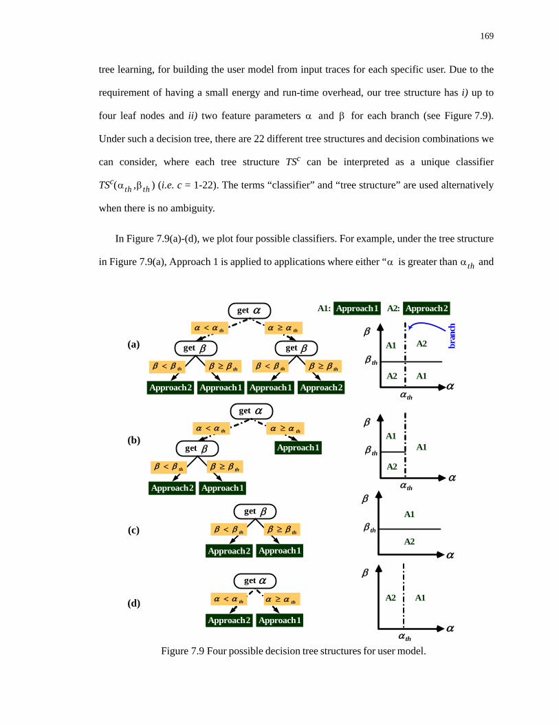
169

tree learning, for building the user model from input traces for each specific user. Due to the

requirement of having a small energy and run-time overhead, our tree structure has i) up to

four leaf nodes and ii) two feature parameters and for each branch (see Figure 7.9).

Under such a decision tree, there are 22 different tree structures and decision combinations we

can consider, where each tree structure TSc can be interpreted as a unique classifier

TSc( , ) (i.e. c = 1-22). The terms “classifier” and “tree structure” are used alternatively

when there is no ambiguity.

In Figure 7.9(a)-(d), we plot four possible classifiers. For example, under the tree structure

in Figure 7.9(a), Approach 1 is applied to applications where either “ is greater than and

α β

αth βth

get α

get β

αget

thαα ≥α thαα <

α thββ ≥α thββ <α thββ ≥α thββ <

Approach 2Approach 1Approach 1Approach 2

Get get β

α thββ ≥α thββ <

Approach 1Approach 2

get

αα


α

thαα ≥thαα <

get α

get β

αα thαα <

α thββ ≥α thββ <

Approach 1


β

thαα ≥

α

β

thα

thβ

Approach 2A2:Approach 1A1:

A2

A1

A1

A2

α

β

thα

thβ A1A1

A2

α

β

thβA1

A2

α

β

thα

A1A2

bran

ch

Figure 7.9 Four possible decision tree structures for user model.

(a)

(b)

(c)

(d)

α αth

170

is smaller than ”, or “ is smaller than and is greater than ”. If we use the

structure in Figure 7.9(d), then the critical application decision is made only depending on

values.

While the sequences of events vary a lot for different users (see Figure 1.5, where the

number and type of applications running on the system are quite different), the specific tree

structures should be learned to fit a certain user. We denote the collected/given sessions3 for

any user ui as the training dataset ( ), while the future (or unseen) sessions as the testing

dataset ( ). The goal of the model learning process is to a find a tree structure ST and the

related threshold value, and/or , such that the communication energy consumption for

future user sequences in is minimized. Since the dataset is not given in advance, we

can only target the sessions in ; that is,

Given sessions in ,

Find a tree structure TSc and corresponding parameters which minimize:

(7.18)

where is the length of session si

c = 1- 22, and = 0.1, 0.2,...0.9

It has been observed that, the performance of the training set is not a good indicator of

predictive performance of the unseen data due to the problem of over-fitting [56]. More

precisely, Efron in [56] proposes a cross-validation method for minimizing the future

prediction error. Here, we first explain the k-fold cross-validation method [92] and then

3. A session is a sequence of events when users log in and log off the system. As shown in Figure 1.5,every duration from the positive clock edge to the negative clock edge is referred to as an event.

β βth α αth β βth

αth

Dtrui

Dteui

αth βth

Dteui Dte

ui

Dtrui

Dtrui

αthc βth

c,( )

min Ecomm_total TsiTSc αth

c βthc,( ),⎝ ⎠

⎛ ⎞

si in Dtr

ui∀

∑⎩ ⎭⎪ ⎪⎨ ⎬⎪ ⎪⎧ ⎫

Tsi

αth βth

171

provide the pseudo code of our tree-based learning process with and without cross-

validation.

In the k-fold cross-validation, the training dataset Dtr is randomly partitioned into k

mutually exclusive subsets (called folds) D1, D2,..., Dk of approximately equal sizes. Each

classifier TS( , ) is trained and tested k times; each time t {1, 2, ..., k}, the classifier is

trained on D-Dt and tested on the validation set Dt. The performance of this classifier is

measured by the average testing results on the validation set Dt, t=1~k. The cross-validation

example with k = 4 is shown in Figure 7.10 where the validation sets are indicated by the gray

blocks. For each classifier TS, we train with (D2,D3,D4), (D1,D3,D4),(D1,D2,D4),(D1,D2,D3)

and test on D1,D2,D3, and D4, respectively. The goal is to find a classifier such that the

average testing results on the validation sets are the best.

Figure 7.11 (a) and (b)(c) illustrate the pseudo code of the structure learning process

without and with cross-validation, respectively. The sub-function find_para takes as inputs D

and TSc, and it returns the parameters for classifier c and its corresponding

performance results, Emin. The k-fold cross-validation method works as we train on D-Dt (see

line 3 in Figure 7.11(b))and test on the validation set Dt (see line 4 in Figure 7.11(b)) for t = 1 -

k.

Of note, the complexity of the k-fold cross-validation approach depends on several

parameters, such as the value k, the model selection with related factors and the amount of

αth βth ∈

Figure 7.10 4-fold cross-validation for model learning.

D1 D2 D3 D4

D1 D2 D3 D4

D1 D2 D3 D4

D1 D2 D3 D4

t = 1

t = 2

t = 3

t = 4

training set

validation set

Dtr

αthc βth

c,( )

172

Figure 7.11 (a) Pseudo codes of tree structure learning process withoutcross-validation method and (b)(c) with cross-validation method.

01: 02: for = 0.1 : 0.1 : 0.903: for = 0.1 : 0.1 : 0.904:

05: if

06: do

07:

08: return

find_para Dateset D classifier TSc,( )

Emin ∞←

αthβth

Etmp Ecomm_total TsiTSc αth βth,( ),⎝ ⎠

⎛ ⎞ si in D∀∑←

Etmp Emin<

Emin Etmp←

αthc βth

c,( ) αth βth,( )←

αthc βth

c Emin, ,

01: for c=1 : 1 : num_classifier 02:

03: select one classifier c’, s.t. minimize 04: output: learned model

TSDtr

c αthc βth

c,( ) Ec,⎝ ⎠⎛ ⎞ find_para Dtr TSc,( )=

Eallc′

TSc′ αthc′ βth

c′,( )

(a) structure learning without cross validation

01: for c=1 : 1 : num_classifier 02: for t = 1 : 1 : k03: 04:

05: select one classifier , minimize

06:

07: output: learned model

TSDtr Dt–c αth

c βthc,( ) Ec,⎝ ⎠

⎛ ⎞ find_para Dtr Dt– TSc,( )=

Eallc 1

k--- Ecomm_total Tsi

TSDtr Dt–c αth

c βthc,( ),⎝ ⎠

⎛ ⎞

si in Dt∀∑

t 1=

k

∑=

c″ Eallc″

TSDtr

c″ αthc″ βth

c″,( ) Ec,⎝ ⎠⎛ ⎞ find_para Dtr TSc″,( )=

TSc″ αthc″ βth

c″,( )

(b) structure learning with k-fold cross-validation

(c) subfuntion find_para( )

173

training data we have (i.e. the number of sequences of events we collect). For k, 10 is a widely

suggested value [56]. In terms of the amount of training data, intuitively, the more, the better.

If the user learning process does not have any memory or runtime limitation, then we can use

all collected data or even apply bootstrap method [56] which can increase the model accuracy.

In practice, however, we need to carefully select all the parameter settings. We report the

overhead in Section 7.7.3 for our system environment.


In Section 7.7.1, we evaluate the hybrid approach consisting of Approaches 1 and 2 under

the pre-defined user model (stage 2 in Figure 7.3). We first evaluate two sub-problems, P1 and

P4, which have an optimal solution; later, the methodology combining P1-P4 at stage 2 is

evaluated. In Section 7.7.2, the energy overhead of running our run-time algorithms is

evaluated for real applications. Finally, the performance of the on-line user model learning

process in stage 3 is reported in Section 7.7.3.

7.7.1. Evaluation on Random Applications

We first evaluate the solution quality of region forming and application mapping

algorithms against the optimal solution. The experiments are performed on an AMD

Athlon™ 64 Processor 3000+ running at 2.04GHz; the results are shown in Figure 7.12.

Twenty categories of random applications are generated with TGFF [162]; these are

combinations of ‘ACG density with 30%, 50%, 70%, 90%’ and ‘variance of communication

rate per edge in one application of 10, 102, 103, 104, and 105’. Each category contains 50

applications with the number of vertices in a ACG ranging from 8 to 12 and assume each

vertex has the same computation requirement. The ACG density of an application is defined as

174

the number of edges in the application divided by the total number of edges in the complete

graph (in which each pair of vertices is connected by an edge). For instance, the ACG density

of an application in Figure 7.6 with 7 vertices and 9 edges is 9/21×100% = 42.8%.

Figure 7.12(a) gives the communication energy consumption under the region forming

algorithm (P1) by comparing it against the optimal solution (i.e., internal communication cost

minimized without any boundary constraint). Figure 7.12(b) compares the communication

energy consumption of the application mapping algorithm (P4) against the optimal solution

for a given region obtained from the region selection algorithm (P3) and the size of the region

is the same as the vertex number in that ACG. Simulation takes around 3 minutes to get the

optimal solution for each application; this is clearly inadequate for a run-time solution. In

contrast, our algorithms for P1 and P4 takes less than 1 microsecond. As shown in

Figure 7.12(a)-(b), the loss in communication energy consumption is less than 12% compared

to optimal solution for all categories, and about 4.5% and 6.2% communication energy loss,

on average, in Figure 7.12(a) and (b), respectively.

ACG density (%)

10 510 4 10 3 10 2 10 1

Variance of comm.

rate per edge

Com

m. e

nerg

y lo

ss p

erce

ntag

e

Figure 7.12 Communication energy loss compared to the optimal solution for (a) regionforming (P1) sub-problem and (b) application mapping (P4) sub-problem on a 2D-mesh NoC.

(a) (b)

Com

m. e

nerg

y lo

ss p

erce

ntag

e

10 510 4 10 3 10 2 10 1

Variance of comm.

rate per edgeACG density (%)

175

Next, we evaluate the stage 2 of the entire methodology as shown in Figure 7.3. Assume

that 10 different applications can be invoked by an user and their ACGs have been generated

with the number of vertices in each application ranges from 3 to 10 and the execution time of

applications ranges from 5 to 30 seconds. Next, we use probabilities to capture the user

behavior. More precisely, we randomly generate the first 100 events; after that, events come

out according to the occurrence probability of all previous events. Events displayed in

Figure 7.13 start from the 101st event sequence. The events are executed on a platform with

8 × 8 processors, one of them being the master PE. The pre-defined user model we use is the

same as the structure in Figure 7.9(b) with and set to 0.8 and 0.7, respectively;

these threshold values fit the best all the data collected from various user sequences). The

communication cost at time t is computed with the total communication energy consumed by

all applications running in the system, over a period from time t-1 to time t.

In Figure 7.13(a), we denote the communication cost of the hybrid approach by “cost_3”,

while the communication cost with Approaches 1 and 2 is denoted by “cost_1” and “cost_2”,

respectively. For the hybrid approach, the process starts taking the user behavior into

consideration after time 20, while the iteration, iter (see Figure 7.4), is set to 3. Note that, the

information of an application leaving the system is not displayed in the figure.

As shown in Figure 7.13(a), with user behavior considered, the energy overhead at

start is less than that when a deterministic approach is applied. As shown, Approach 1

performs well initially since the system utilization is low. As the system utilization

increases, Approach 1 performs poorly since there are many non-contiguous regions in

the system. One can also see that the communication cost ratio does not fluctuate

significantly after the system runs for a certain period of time. We estimate that the

hybrid approach achieves about 40% and 25% communication energy savings, compared

αth βth

176

to approaches 1 and 2, respectively. We also compare the L(R) metric, where R is the

available/unused resources in the system at each time unit among different approaches. We

denote the L(R) of the hybrid approach by “L_3”, while the L(R) with Approaches 1 and 2 are

denoted by “L_1” and “L_2”. In Figure 7.13(b), we plot the ratio of L_3/L_1, L_3/L_2, and

the number of applications in the system at each time unit. As shown in Figure 7.13(b), the

L(R) of the hybrid approach is less than 10% greater than that of Approach 2, which implies

:

:

:

: L_3 / L_1: L_3 / L_2: # of applications in the system

1110987654321

1110987654321

0 50 100 150

1110987654321

Figure 7.13 (a) Communication cost comparison among Approach 1, Approach 2, and thehybrid approach (which considers the user behavior) on an 8 × 8 NoC. (b) L(R) where R isthe available/unused resources comparison among Approach 1, Approach 2, and thee hybridapproach.

0 50 100 150

0.4

0.6

0.8

1

1.2

1.4

:::

cost_3 / cost_2cost_3 / cost_1

event trigger

time (sec)

com

mun

icat

ion

ratio

time (sec)

L(R

) rat

io

# of

app

licat

ions

(a)

(b)

L_1/L_3L_2/L_3

177

that the external contention in hybrid approach is not so serious. In addition, when the system

utilization is higher (i.e. more applications are present in the system), it can be observed that

L(R) in Approach 1 is much higher than that in hybrid approach; this is because, when the

application leaves the system, there is always a scattered region left in the system

configuration.

To show the scalability of our proposed methodology, we report the communication

consumption comparison among these three approaches on different size NoCs, i.e. 6 × 6,

8 × 8, 10 × 10, and 12 × 12 as shown in Table 7.2. The communication cost of running

applications on each NoC for a certain approach is obtained when the ratio does not fluctuate

significantly, i.e. after the system runs for a certain period of time (similar to the case in

Figure 7.13(a)). As observed, the ratio decreases as the size of the platform increases,

which shows that our hybrid approach looks promising particularly for large NoC

platforms.

7.7.2. Real Applications with Run-time Energy Overhead Considered

In this section, we apply our proposed methodology to real applications, i.e. the embedded

system benchmark suite (E3S) [50]: Automotive/Industrial, Consumer, Networking, Office

automation, and Telecom. Our homogeneous 5 × 5 mesh-based NoC contains 24 slave

processors (some are AMD ElanSC520 operating at 133 MHz, some are AMD K6-2E

Table 7.2 Comparison of communication consumption among different approaches on a different size NoCs.

communication ratio 6 × 6 8 × 8 10 × 10 12 × 12cost_3/cost_1 0.74 0.60 0.48 0.32cost_3/cost_2 0.81 0.75 0.71 0.63

178

operating at 500 MHz) and one master PE, MicroBlaze core (100MHz) acting as the global

manager.

A C++ simulator using the bit energy metric model in [170] evaluates the

communication energy consumption where is set to 4.49 × 10-13 (Joule/bit) and

contains the energy consumes on the routing engine (10-13 Joules/packet), arbiter request

(1.155 × 10-12 Joules/packet), switch fabric (2.84 × 10-13 Joules/bit), and buffer reading and

writing (1.056 × 10-12 and 2.831 × 10-12 Joules/bit, respectively).

Five benchmarks of E3S have been partitioned off-line [30][127]. As such, the number of

vertices in the ACG of each benchmark ranges from 3 to 8 and vertices have two different of

computation capacity level where critical vertices must be operate at AMD K6-2E for meeting

the application deadline. The user sequences come from realistic data collected from five

different applications running under Windows XP. The execution time of an event is

normalized to the reasonable range from 10 μs to 10 ms for E3S benchmarks. We run 200

events (from the 101st to the 300th event) for each scenario: “Nearest Neighbor [27]”,

“Approach 1”, “Approach 2”, and “Hybrid approach”. For “Approach 1” and “Approach 2”

scenarios, we only apply approach 1 and approach 2, respectively, to all events (see

Figure 7.4). For the “Hybrid approach” scenario, approaches 1 and 2 are selected at run-time

(the iteration, iter (see Figure 7.4) is set to 3) based on the pre-defined user model in

Figure 7.9(b), with and set to 0.8 and 0.7, respectively. Of note, “Approach 2” and

“Hybrid approach” correspond to stages 1 and 2 in Figure 7.3, respectively.

In the following evaluation, we consider the run-time and energy overhead of processing

our proposed algorithms: i) running the approach selection process (i.e., , compared to

, ) on the manager, ii) running the resource assignment process (i.e., P1-P2 for

Approach 1 and P3-P4 for Approach 2) and iii) sending the control messages over the control

network back to the manager. Of note, the communication volume for all control messages in

Elink ERbit

αth βth

α β

αth βth

179

one event is Z = [a bits (for showing the location of the slave processor, which depends on

network size) + 1 bit (resource status)] × MD (distance of all slave processors to the master

PE). Of note, compared to the data messages transmitted for real applications (which is in the

order of Megabits), the overhead of sending control messages is clearly negligible.

To compare the communication energy consumption for each scenario, we denote some

variables as follows:

• : the communication energy consumption of an event Q, or an application Q, in

scenario x.

• :the energy overhead of running the approach selection and resource

assignment processes on the master PE for the event Q in scenario x.

• :the run-time overhead of running the approach selection and resource

assignment processes on the master PE for the event Q in scenario x (obtained from

MicroBlaze processor running on Xilinx Vertex-II Pro XC2VP30 FPGA).

We set the scenario “Nearest Neighbor [27]” as the baseline algorithm and we assume

zero energy and run-time overhead for the baseline algorithm. Then the total communication

energy consumption for these 200 events in scenario x is:

[ ]

The experimental results are shown in Table 7.3. We determine experimentally that for

the “Hybrid approach”, about 60% communication energy savings can be achieved compared

to “Nearest Neighbor” scenario.

EApp Qx

EApp Qx_select

TApp Qx_select

Q 101=

300

∑ EApp Qx

Ex_select

App Q+

180

When comparing with “Approach 1” and “Approach 2” schemes, the “Hybrid approach”

provides around 38% and 24% communication energy savings, respectively. The average run-

time overhead of the approach selection and resource assignment processes in “Approach

1”, “Approach 2”, and “Hybrid approach” scenarios for one event is 47.2μsec, 49.4μsec, and

53.4μsec, respectively. As the hard deadline of E3S benchmarks are in msec order, our

algorithms are appropriate to be done at run-time.

7.7.3. Real Applications with On-line Learning of User Model

Here, we evaluate the performance with the on-line user model. In this implementation,

we include a Multimedia System (MMS) [80], a Video Object Plane Decoder [104], and

the five E3S benchmarks [50]; the number of vertices in the ACG of each benchmark

ranges from 5 to 25. Four scenarios (Nearest Neighbor [27], stages 1, 2, and 3 in Figure 7.3)

are considered for the system configuration of a 10 × 10 mesh network. For stage 3, 10-fold

cross-validation method is used for learning the user model [56]. As discussed in Section 2.3.1

for capturing the essence of human behavior while users interact with computing systems, the

user sequences come from collecting the behaviors of four users running seven

applications (i.e. Media player, Windows explorer, Windows powerpoint, Matlab, Adobe

acrobat, Microsoft word, and Outlook express) in a Windows XP environment; the

execution time is normalized, ranging from 10 μs to 100ms.

Table 7.3 Comparison of the run-time overhead and the overall communication energy savings under four implementations on a 5 × 5 mesh NoC.

Approach Tx_selection, orAvg. run-time overhead

per event (μsec)Normalized

total event costNearest Neighbor [27] 0 1

Approach 1 47.2 0.682Approach 2 (stage 1) 49.4 0.551

Hybrid approach (stage 2) 53.4 0.405

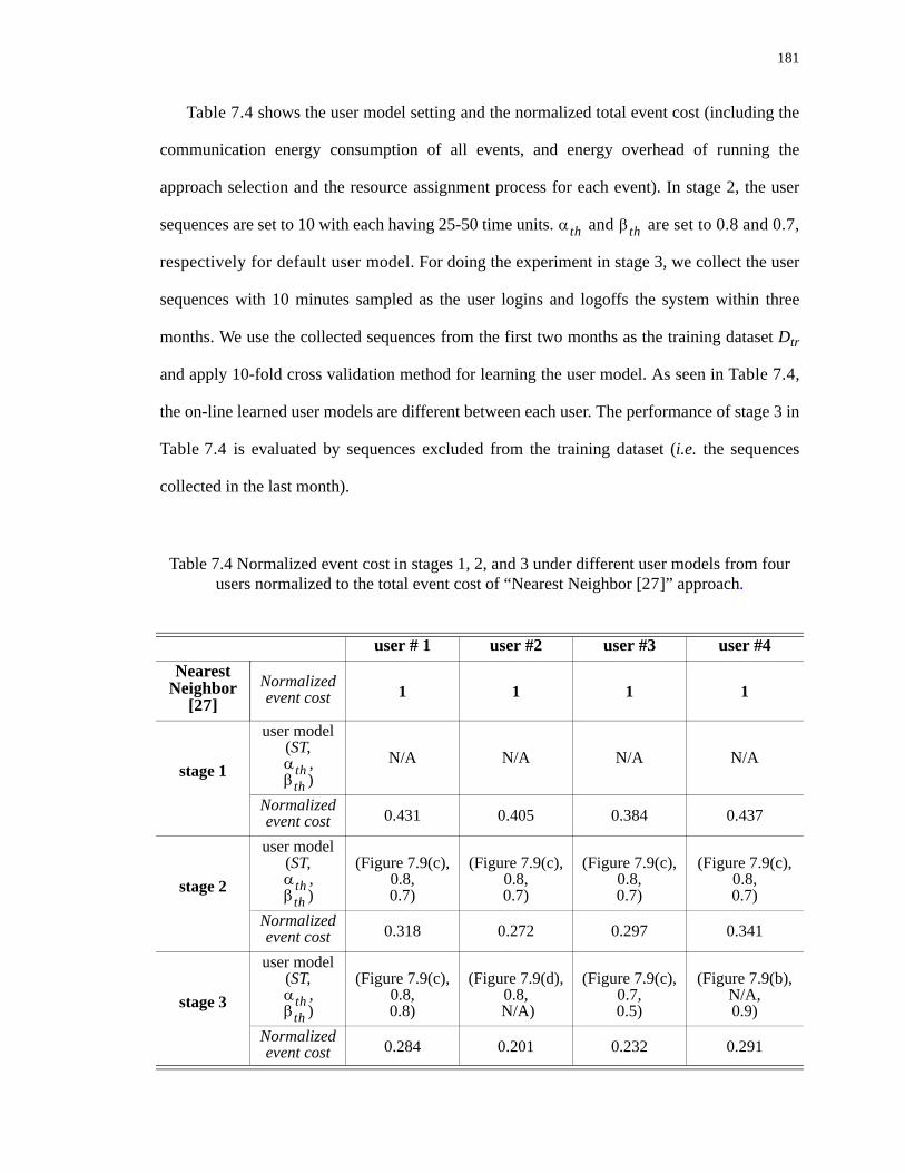
181

Table 7.4 shows the user model setting and the normalized total event cost (including the

communication energy consumption of all events, and energy overhead of running the

approach selection and the resource assignment process for each event). In stage 2, the user

sequences are set to 10 with each having 25-50 time units. and are set to 0.8 and 0.7,

respectively for default user model. For doing the experiment in stage 3, we collect the user

sequences with 10 minutes sampled as the user logins and logoffs the system within three

months. We use the collected sequences from the first two months as the training dataset Dtr

and apply 10-fold cross validation method for learning the user model. As seen in Table 7.4,

the on-line learned user models are different between each user. The performance of stage 3 in

Table 7.4 is evaluated by sequences excluded from the training dataset (i.e. the sequences

collected in the last month).

Table 7.4 Normalized event cost in stages 1, 2, and 3 under different user models from four users normalized to the total event cost of “Nearest Neighbor [27]” approach.

user # 1 user #2 user #3 user #4Nearest

Neighbor [27]

Normalizedevent cost 1 1 1 1

stage 1

user model(ST,

,)

N/A N/A N/A N/A

Normalizedevent cost 0.431 0.405 0.384 0.437

stage 2

user model(ST,

,)

(Figure 7.9(c), 0.8, 0.7)

(Figure 7.9(c), 0.8, 0.7)

(Figure 7.9(c), 0.8, 0.7)

(Figure 7.9(c), 0.8, 0.7)


stage 3

user model(ST,

,)

(Figure 7.9(c),0.8,0.8)

(Figure 7.9(d),0.8,

N/A)

(Figure 7.9(c),0.7,0.5)

(Figure 7.9(b), N/A,0.9)


αth βth

αthβth

αthβth

αthβth

182

As observed in Table 7.4, with the pre-defined user model considered (stage 2), we

achieve 70%, on average, communication energy savings compared to the “Nearest

Neighbor” schemes. With learned user model (stage 3), we can achieve 18% and 75%, on

average, communication energy savings compared the pre-defined user model scheme

and the “Nearest Neighbor” schemes, respectively4. While experimenting on the user

model learning procedure for the training dataset Dtr without 10-fold cross-validation

method, we observe that the energy consumes 15% more on the testing dataset, on

average, for each user compared to user model learning with cross-validation method

applied.

Of note, the overhead of the model learning step is not included in Table 7.4 since the

learning step is not executed for each event. Basically, we collect hundreds of sequences from

one user for a period of time and update the user model once for that user if necessary. The

overhead of learning the user model is affected by multiple factors, i.e. the user model

complexity (including the parameters and the structure for building the model), the amount of

collected sequences (how often for updating the model), and the computation capability of the

global manager.

Here, we report that the run-time overhead of the learned user model process (steps in

Figure 7.11 (b)) running on 100MHz MicroBlaze processor with the collected user sequences

(sessions with 10 minutes sampled as the user login and logoff the system for three months)

without and with the cross-validation process are 1.3 second and 9.6 seconds. The user model is

learned from 22 different decision trees (or classifiers) combined with different and

values ranging from 0.1, 0.2,...,to 0.9, while using the 10-fold cross-validation. We

conclude that having the cross-validation process for the learning process indeed helps

4. For example, in the MIT RAW on-chip network where the communication energy consumption rep-resents 36% of the total energy consumption [20], applying our approach in stage 3 of Figure 7.3can save 27% of total energy consumption compared to the “Nearest Neighbor” scheme.

αth βth

183

build more accurate user model, but we need to evaluate its run-time overhead. Therefore,

in reality, there is no restricted rule of when, where, and even how to update the user model. It

is suggested to do some analysis to see whether or not the current user behavior is suitable for

the latest updated user model. In addition, we could update the model slightly (e.g. modifying

the thresholds only) instead of learning the model using whole collected sequences. Moreover,

for future embedded systems, the user model learning process is not necessary to be built on

the system itself. We could upload the collected sequences periodically to the data center and

with its strong computation capacity, we are able to build more accurate model before

downloading relevant parameters back to the system.

The proposed tree-based structure for building user model on-line for each specific user is

the first step for run-time optimization while taking the user behavior into consideration. More

work needs to be done by increasing the adaptability of the system while considering the

feedback between system and users. In addition, if one user with his/her behavior has hugh

difference for certain reasons (as shown in Figure 1.1, the dot changes from one cluster to

other clusters), it is suggested to either include heavier run-time optimization such that the

system can better adapt to this user, or suggest the user to own new platform which can fit

him/her well with light-wight optimization.

7.8. Summary

In this chapter, we have proposed a run-time strategy for allocating the application tasks to

embedded MPSoC platform where communication happens via the NoC approach. As novel

contribution, we have incorporated the user behavior information in the resource allocation

process; this allows system to better respond to real-time changes and adapt dynamically to

different user needs. Several algorithms have been proposed for solving the task allocation

problem, while minimizing the communication energy consumption and network contention.

184

By applying machine learning techniques, more precisely tree-based model learning, for building

the user model from input traces, we can achieve around 75.8% communication energy savings

compared to an arbitrarily contiguous allocation scenario on the NoC platform. As suggested,

although we focus on the 2-D mesh NoC platform, our algorithm can be adapted to other

regular architecture with different networks topologies.

It can be seen that the methodology proposed in this chapter can be applied to embedded

system in the second and third categories as discussed in Table 1.1. For the systems in the first

category, we are also interested in researching the patterns of human dynamics which allow us

to follow specific human actions in ultimate detail, such as adding the social behavior

component (flow experience). This remains to be done in future work (see Table 8.2.2).

185

8. CONCLUSIONS AND FUTURE DIRECTIONS

With industry shifting to platform-based embedded system design, much progress in the

traditional DSE techniques has been moving from task-level, resource-level, to even system-

level perspective, while targeting system optimization with the goal of improving the system

performance. Over recent years, embedded systems have gained an enormous amount of

processing power and functionality; future systems will likely consist of tens or hundreds of

heterogeneous cores supporting multiple applications. However, from users’ perspective,

users purchase “fit enough” products which typically provide “just-enough performance”

during operation, and rather focus on additional concerns, such as the appearance,

practicability of the product, or even price. In addition, due to the high variability seen in user

preferences, it becomes much more challenging for system designers to meet the various users

taste.

8.1. Dissertation Contributions

In this dissertation, we propose a unified user-centric embedded design framework for

both off-line DSE and on-line optimization, while explicitly involving the user experience into

the process. In other words, we target incorporating the user behavior information into the

system design, optimization, and evaluation steps. The main contributions of this dissertation

can be summarized as follows:

• For MPSoCs with predictable system configurations, the platform can be generated

following the traditional Y-chart design flow, given the universal use-cases application

parameters, and architecture templates. In Chapter 3, we explored the system

186

interconnect for large MPSoC design using the NoC communication approach, which

aims at trading off the system performance and several physical design metrics. The

results demonstrated that the optimization framework is capable of obtaining Pareto

solutions with multiple buses instead of the current single bus that significantly reduces

communication latency with negligible fabric wirelength and area penalty.

• Satisfying the end user is the ultimate goal of any system optimization. Toward this end,

in Chapter 4, we presented a new design methodology for automatic regular platform

generation of embedded NoCs resulting in unpredictable system configurations, while

including explicitly the information about the user experience into the design process;

this aims at minimizing the workload variance and allows the system to better adapt to

different types of uses. More precisely, we relied on machine learning techniques to

cluster the traces from various users into several classes, such that the differences in

user behavior for each class are minimized. Then, for each cluster, we proposed an

architecture automation deciding the number, the type, and the location of resources

available in the platform, while satisfying various design constraints.

• Exploring on-line resource allocation techniques while mapping multiple applications

onto multiple computing resources is a fundamentally important issue in MPSoC

design. This also belongs to the large class of resource allocation problems in parallel

systems. In Chapter 5, efficient techniques for run-time application mapping onto

NoC platforms with multiple voltage levels have been presented with the goal of

minimizing the total communication energy consumption and maximizing the

system performance, while still providing the required performance guarantees. In

parallel, the proposed techniques allow for new applications to be easily added to

the system platform with minimal inter-processor communication overhead.

187

• The collective resource utilization and system reliability are important for achieving

overall computing capacity in MPSoCs. Especially, for larger MPSoCs integrated with

hundreds or thousands cores where the communication happens via the NoC approach,

any failures through the computation or communication components may degrade the

system performance, or even render the whole system useless. In Chapter 6, we

discussed the workload variation resulting from the system itself and later investigated

the spare core placement problem taking into account the with fault-tolerant property.

As the main theoretical contribution, we addressed the resource management problem on

irregular NoC platforms where permanent, transient, and intermittent faults can appear

statically or dynamically in the system. A fault-tolerant application mapping algorithm

has been presented which allocates the application tasks to the available, reachable, and

defect-free resources with the goal of maximizing the overall system performance.

• Due to variations in users’ behavior, the workload across different resources may

exhibit high variability even when using the same hardware platform. In Chapter 7,

extensible and flexible run-time resource management techniques have been presented

that allow systems to respond much better to run-time changes. In addition, we

proposed light-weight machine learning techniques for learning the user model at run-

time such that the systems are able to adapt dynamically to user needs. Given the

application characteristics, the on-line learned user model, and current system

configuration, our algorithm assigned the dynamic application tasks to the appropriate

resources such that the overall system performance is maximized. It has been

experimentally demonstrated that considering the user behavior during the resource

management process has an important impact on the system performance improvement.

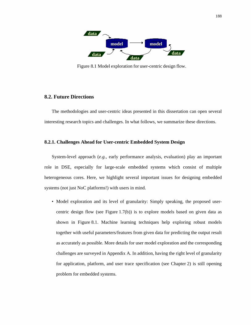
188

8.2. Future Directions

The methodologies and user-centric ideas presented in this dissertation can open several

interesting research topics and challenges. In what follows, we summarize these directions.

8.2.1. Challenges Ahead for User-centric Embedded System Design

System-level approach (e.g., early performance analysis, evaluation) play an important

role in DSE, especially for large-scale embedded systems which consist of multiple

heterogeneous cores. Here, we highlight several important issues for designing embedded

systems (not just NoC platforms!) with users in mind.

• Model exploration and its level of granularity: Simply speaking, the proposed user-

centric design flow (see Figure 1.7(b)) is to explore models based on given data as

shown in Figure 8.1. Machine learning techniques help exploring robust models

together with useful parameters/features from given data for predicting the output result

as accurately as possible. More details for user model exploration and the corresponding

challenges are surveyed in Appendix A. In addition, having the right level of granularity

for application, platform, and user trace specification (see Chapter 2) is still opening

problem for embedded systems.

Figure 8.1 Model exploration for user-centric design flow.

model

data

datadata

model

data

189

• Human Dynamics: Systems are designed for humans. Exploring human dynamics helps

capturing individual human behavior and following specific human actions in ultimate

detail. Several study on human dynamics are already available, such as heavy tailed

distribution (also known as power law distribution) [11][69][70][163]. However, it is

still an open problem as to how one can incorporate human activity patterns in

embedded systems design.

• Workload Fidelity: Due to the user preference variation, it is required to understand the

buyer-to-be’s workload of target applications before designing a system [52]. Chen et

al. develop a workload analysis: recognition, mining, and synthesis (RMS) to model

events, objects, and concepts cased on end-user inputs which can be applied to

embedded systems, gaming, graphics, and even financial analytics [33]. With well

understanding of the workloads from different users, we could come out with the right

level of granularity for application specification, and later capture the main scenario for

system configuration for each specific user.

User-centric research for embedded systems is still at an early stage, and there is much

work that needs to be carried out, from modeling the user behavior, to analysis of various

workloads, and to user-aware DSE and optimization. However, we believe that making users

part of the design process is crucial for embedded systems design as this can lead to better and

more flexible designs in the future.

8.2.2. Increasing Flow Experience by Designing Embedded Systems

We argue that future embedded systems need to be designed using a flexible user-centric

design methodology geared primarily toward maximizing the user satisfaction (i.e., flow

experience) rather than only optimizing performance and power consumption. Therefore,

compared to the traditional design, we aim at re-focusing the current design paradigm by

190

placing the user behavior at the center of the design process and by using psychological

variables such as user ability and motivation as the main drivers of this process. This allows

systems to become more capable of adapting to different users' needs and of enhancing short-

and long-term user satisfaction.

Generally speaking, the flow experience is a mental state in which an individual feels

completely immersed in the task or activity at hand. Think, for instance, of web browsing.

While in flow, the user experiences enhanced motivation, concentration, positive affect, and

task involvement [45]. Theoretically, an individual achieves a state of flow when his/her

abilities match the challenges faced when engaged in executing a particular task. It has been

observed that designing interfaces that favor flow experiences helps increase the usability of

the information technology in use. Moreover, the increased user motivation experienced

during a flow episode guarantees continued use of technology and enhanced return behavior

[124].

Prior work in psychology indicates that while each task or application makes users feel

more or less stimulated, the optimal level of motivation (i.e., the flow experience) is achieved

by challenging tasks that match the user's abilities as seen in Figure 8.2 [45][167]. Indeed, if

the level of challenge presented by an application is low and does not engage the user, then the

user can quickly lose interest and get relaxed or even become bored by that particular activity

(see zones III and IV in Figure 8.2). However, if the task challenge is beyond the user's current

ability, then the activity becomes overwhelming and the user may feel frustrated or even

anxious (zone I in Figure 8.2). As shown in Figure 8.2, the flow zone (zone II) is reached only

when the task is challenging and the user's skills are great enough to deal with it; when

achieving a flow experience, the individual truly finds pleasure in doing the current activity

[45][147].

191

Therefore, from previous psychological research, mapping the relationship between the

task difficulty and the level of user ability is very important in predicting flow experience.

Applying this work to the embedded system design process, the experience of anxiety or

relaxation should prompt designers to either change the level of challenge in the system (e.g.,

CPU) or to motivate the user to increase his/her skill level in order to re-experience the flow

[147]. Thus, in order to maximize user flow experience, the traditional design paradigm needs

to be redefined by taking into consideration psychological variables such as user ability and

positive affect.

Looking forward, we believe that enhancing the users; flow experience offers a new

paradigm for understanding both individual and collective human functioning and

consequently plan to explore its implications for user-centric DSE of embedded systems.

Motivation and preliminary results are reported in [43]. We are hopeful that the future design

process will take into account the human nature of users and their ever-changing abilities and

interests.

Figure 8.2 Four-quadrant states in terms of challenge and skill level.

Skill Level

Cha

lleng

e Le

vel

I. Anxiety II. Flow

III. Boredom IV. Relaxation

Skill Level

Cha

lleng

e Le

vel

I. Anxiety II. Flow

III. Boredom IV. Relaxation

193

Bibliography

[1] H. Abdel-wahab, et al., “A proportional share resource allocation algorithm for real-time, time-shared systems,”

Proc. Real-Time Systems Symposium, 1996, pp. 288-299.

[2] S. N. Adya and I. L. Markov, “Fixed-outline floorplanning: enabling hierarchical design,” IEEE Trans. on VLSI

Systems, vol 11(6), Dec. 2003, pp. 1120-1135.

[3] R. Alur, D. L. Dill, “A theory of timed automata,” Theoretical Computer Science, 1994, vol. 126, pp. 183-235.

[4] G. Ascia, V. Catania, M. Palesi, “Multi-objective mapping for mesh-based NoC architectures,” Proc. Hardware/

Software Codesign and System Synthesis (CODES+ISSS), Sept. 2004, pp.182-187.

[5] G. Ascia, V. Catania, M. Palesi., “A multi-objective genetic approach to mapping problem on Network-on-Chip,”

Journal of Universal Computer Science, vol. 12, no. 4, 2006, pp. 370-394.

[6] A. Avd, “1.1 Billion Cell Phones Sold Worldwide In 2007, Says Study,” http://www.switched.com/2008/01/25/1-

1-billion-cell-phones-sold-worldwide-in-2007-says-study/.

[7] A. Baghdadi, et al., “An efficient architecture model for systematic design of application-specific multiprocessor

SoC,” Proc. DATE, 2001, pp. 55-63.

[8] F. Balarin, et al. Hardware-Software Co-design of Embedded Systems - The POLIS approach. Kluwer Academic

Publishers, 1997.

[9] N. Banerjee, P. Vellanki, K. S. Chatha, “A power and performance model for Network-on-Chip architectures,”

Proc. DATE, 2004, pp. 1250-1255.

[10] S. Bani-Mohammad, M. Ould-Khaoua, I. Ababneh, L. M. Mackenzie, “An efficient processor allocation strategy

that maintains a high degree of contiguity among processors in 2D mesh connected multicomputers.” Proc.

Computer Systems and Applications, 2007, pp. 934-941.

[11] A.-L. Barabási, “The origin of bursts and heavy tails in human dynamics,” Nature 435, 2005, pp. 207-211.

[12] M. Barr, “Architecting embedded systems for add-on software,” Embedded Systems Programming, Sept. 1999,

pp. 49-60.

[13] Bell, E. T. “Exponential Numbers” Amer. Math. Monthly 41, 1934, pp. 411-419 .

[14] C. M. Bender, M. A. Bender, E. D. Demaine, S. P. Fekete, “What is the optimal shape of a city?,” Journal of

Physics A: Mathematical and General, vol. 37, 2004, pp. 147-159.

[15] M. A. Bender, et al., “Communication-aware processor allocation for supercomputers,” Proc. Workshop on

Algorithms and Data Structure, Aug. 2005, pp. 169-181.

[16] C. M. Bender, M. A. Bender, E. Demaine, and S. Fekete, “What is the optimal shape of a city?,” Journal of Physics

A: Mathematical and General, vol. 37, 2004, pp. 147-159.

[17] L. Benini, G. De Micheli, “Networks on chip: a new paradigm for systems on chip design,” Proc. DATE, 2002, pp.

418-419.

[18] D. Bertozzi, and A. Jalabert, “NoC synthesis flow for customized domain specific multiprocessor systems-on-

chip,” IEEE Trans. Parallel Distrib. Syst., vol. 16, no. 2, Feb. 2005, pp. 113-129.

194

[19] S. Bertozzi, et al., “Supporting task migration in multi-processor systems-on-chip: a feasibility study,” Proc.

DATE, 2006, pp. 1-6.

[20] P. Bhojwani, et al., “A heuristic for peak power constrained design of network-on-chip (NoC) based multimode

systems,” Proc. VLSI Design, Jan. 2005, pp. 124-129.

[21] C. M. Bishop, Pattern Recognition and machine learning (Information Science and Statistics), 2006.

[22] R. Bitirgen, E. I.pek, and J.F. Martínez, “Coordinated management of multiple resources in chip multiprocessors:

A machine learning approach,” Intl. Symp. on Microarchitecture, Nov. 2008, pp. 318-329.

[23] S. Borkar, “Thousand core chips: a technology perspective,” in Proc. DAC, 2007, pp. 746-749.

[24] R. Burke, “The Wasabi Personal Shopper: a case-based recommender system,” Proc. Artificial intelligence States,

July 1999, pp. 844-849.

[25] I. V. Cadez, et al., “Model-based clustering and visualization of navigation patterns on a web site,” Data Mining

and Knowledge Discovery, 2003, pp. 399-424.

[26] I. V. Cadez, S. Gaffney, P. Smyth, “A general probabilistic framework for clustering individuals and objects,”

Proc. on Knowledge Discovery and Data Mining, Aug. 2000, pp. 140-149.

[27] E. Carvalho, N. Calazans, F. Moraes, “Heuristics for Dynamic Task Mapping in NoC-based Heterogeneous

MPSoCs,” IEEE/IFIP Workshop on Rapid System Prototyping, Porto Alegre, Brazil, May 2007, pp. 34-40.

[28] F. Catthoor, et al., “How can system-level design solve the interconnect technology scaling problem?,” Proc.

DATE, 2004, pp. 332-337.

[29] C. Chang and P. Mohapatra, “Improving performance of mesh connected multicomputers by reducing

fragmentation,” Journal of Parallel and Distributed Computing, vol. 52, no. 1, 1998, pp. 40-68.

[30] J.-M. Chang and M. Pedram, “Codex-dp: co-design of communicating systems using dynamic programming,”

IEEE Trans. Comput.-Aided Des. Integr. Circuits Syst. (TCAD), vol. 19, July 2000, pp. 732-744.

[31] K.S. Chathak, K. Srinivasan, G. Konjevod, “Automated techniques for mapping of application-specific network-

on-chip architectures,” IEEE Trans. Comput.-Aided Des. Integr. Circuits Syst. (TCAD), Aug. 2008, pp. 1425-

1438.

[32] S. Chatterjee, Z. Wei, A. Mishchenko, R. Brayton,“A linear time algorithm for optimum tree placement,” Intl.

Workshop on Logic and Synthesis, 2007.

[33] Y.-K. Chen, et al., “Convergence of recognition, mining, and synthesis workloads and its implications,” Proc. of

IEEE, 2008, pp. 790-807.

[34] P. Chen and K. Keutzer, “Towards true crosstalk noise analysis,” Proc. ICCAD, 1999, pp. 132-138.

[35] C.-L. Chou, R. Marculescu, “Incremental run-time application mapping for homogeneous NoCs with multiple

voltage levels,” Proc. Hardware/Software Codesign and System Synthesis (CODES+ISSS), Oct. 2007, pp. 161-

166.

[36] C.-L. Chou, R. Marculescu, “User-aware dynamic task allocation in Networks-on-Chip,” Proc. DATE, 2008, pp.

1232-1237.

195

[37] C.-L. Chou, U. Y. Ogras, R. Marculescu, “Energy- and performance-aware incremental mapping for Networks-

on-Chip with multiple voltage levels” IEEE Trans. on Computer-Aided Design of Integrated Circuits and Systems

(TCAD), vol. 27, no. 10, Oct. 2008, pp. 1866-1879.

[38] C.-L. Chou, R. Marculescu, “Run-time task allocation considering user behavior in embedded multiprocessor

Networks-on-Chip,” IEEE Trans. on Computer-Aided Design of Integrated Circuits and Systems (TCAD), vol. 19,

no. 1, Jan. 2010, pp. 78-91.

[39] C.-L. Chou, R. Marculescu, “Contention-aware application mapping for Network-on-Chip communication

architectures,” Proc. ICCD, Oct. 2008, pp. 164-169.

[40] C.-L. Chou, R. Marculescu, “User-centric design space exploration for heterogeneous Network-on-Chip

platforms,” Proc.DATE, April 2009, pp. 15-20.

[41] C.-L. Chou, R. Marculescu, “Designing heterogeneous embedded Network-on-Chip with users in mind,” to

appear, IEEE Trans. on Computer-Aided Design of Integrated Circuits and Systems (TCAD), 2010.

[42] C.-L. Chou, R. Marculescu, “Fault-tolerant algorithms for run-time resource allocation in many core systems,”

Proc. Semiconductor Research Corporation (SRC), TECHCON, 2009.

[43] C.-L. Chou, A. M. Miron, R. Marculescu, “Find your flow: Increasing flow experience by designing ‘Human’

Embedded Systems,” to appear, Proc. DAC, 2010.

[44] H. Cook, K. Skadron, “Predictive design space exploration using genetically programmed response surfaces,”

Proc. DAC, 2008, pp. 960-965.

[45] M. Csikszentmihalyi, “Flow: The psychology of optimal experience,” New York: Harper and Row, 1990.

[46] W. J. Dally and C. L. Seitz, “Deadlock-free message routing in multiprocessor interconnection networks,” IEEE

Trans. on Computer, 1987, pp. 547-553.

[47] W. J Dally, B. Towles, “Route packets, not wires: on-chip interconnection network,” Proc. DAC, 2001, pp. 684-

689.

[48] C. Darwin, On the origin of species by means of natural selection, or the preservation of favoured races in the

struggle for life,1859: ISBN 0-451-52906-5.

[49] S. Das, et al, “RazorII: In situ error detection and correction for PVT and SER tolerance,” IEEE Journal of Solid-

State Circuits, Jan. 2009, pp. 32-48.

[50] R. Dick, “Embedded system synthesis benchmarks suites (E3S),” http://ziyang.eecs.umich.edu/~dickrp/e3s/

[51] R. P. Dick, N. K. Jha, “MOGAC: A multiobjective genetic algorithm for hardware-software cosynthesis of

distributed embedded systems,” IEEE Trans. on Computer-Aided Design of Integrated Circuits and Systems

(TCAD), 1998, pp. 920-935.

[52] K. Diefendorff, and P. K. Dubey, “How multimedia workloads will change processor design,” Computer 30, 9,

Sept. 1997, pp. 43-45.

[53] T. Dumitras, S. Kerner, R. Marculescu, “Towards on-chip fault-tolerant communication,” Proc. ASP-DAC, 2003,

pp. 225-232.

[54] Eason, K. Information Technology and Organizational Change. 1st. Taylor & Francis, Inc. 1989.

196

[55] S. A. Edwards, “What do we do with 1012 transistors? The case for precision timing,” DSRC TeraChip Workshop,

2008.

[56] Bradley Efron, “Estimating the error rate of a prediction rule: improvement on cross-validation”, Journal of the

American Statistical Association, vol. 78, no. 382, 1983, pp. 316-331.

[57] Z. Feng, et al., Floorplan representation in VLSI, handbook of DATA structures and applications, by D.P. Mehta

and S. Sahni, Chapman and Hall, 2004, pp. 53-1: 53-29.

[58] C. Ferdinand, R. Wilhelm, “On predicting data cache behavior for real-time systems,” Proc. of the ACM Workshop

on Languages, Compilers, and Tools for Embedded Systems, 1998, pp.16-30.

[59] S. Fuller, RapidIO: The Embedded System Interconnect. ISBN: 0470092912.

[60] M. Geilen, T. Basten, “A calculator for pareto points,” Proc. DATE, 2007, pp. 16-20.

[61] S. V. Gheorghita, et al., “Automatic scenario detection for improved WCET estimation,” Proc. DAC, 2005, pp.

101-104.

[62] S. V. Gheorghita, T. Basten, H. Corporaal, “Application scenarios in streaming-oriented embedded-system

design,” IEEE Design & Test of Computers, vol. 25, no. 6, 2008, pp.581-589.

[63] S. V. Gheorghita, et al., “System-scenario based design of dynamic embedded system,” ACM Trans. on Design

Automation of Electronic Systems (TODAES), vol. 14, no. 1, Jan. 2009.

[64] M. Gomaa, et al., “Transient-fault recovery for chip multiprocessors,” Proc. ISCA, 2003, pp. 98-109.

[65] C. Grecu, et al., “Essential fault-tolerance metrics for NoC infrastructures,” On-Line Testing Symposium, 2007, pp.

37-42.

[66] M. Gries, “Methods for evaluating and covering the design space during early design development,” Integr. VLSI

Journal, 2004, pp. 131-183.

[67] Rebecca E. Grinter, “Systems architecture: product designing and social engineering,” ACM SIGSOFT Software

Engineering Notes, vol. 24, no. 2, 1999, pp.11-18.

[68] A. Gupta, B. Lin, P. A. Dinda, “Measuring and understanding user comfort with resource borrowing,” Proc. High

Performance Distributed Computing, June 2004, pp. 214-224.

[69] Mor Harchol-Balter, “The effect of heavy-tailed job size distributions on computer system design,” Proc. of the

ASA-IMS Conf. on Applications of Heavy Tailed Distributions in Economics, June 1999.

[70] T. Henderson and S. Bhatti, “Modelling user behaviour in networked games,” Proc of Intl. Conf. on Multimedia,

Sept. 2001, pp. 212-220.

[71] A. Hergenhan, W. Rosenstiel, “Static timing analysis of embedded software on advanced processor architectures,”

Proc. DATE, 2000, pp. 552-559.

[72] Y. Hoskote, “A 5-GHz Mesh Interconnect for a Teraflops Processor,” IEEE Micro, vol. 27, no. 5, Sept./Oct., 2007,

pp. 51-61.

[73] http://lava.cs.virginia.edu/HotSpot/

[74] http://src.alionscience.com/

[75] http://www.arm.com/products/solutions/axi_spec.html

197

[76] http://www.sematech.org/docubase/document/3955axfr.pdf

[77] http://www.wavecom.com/.

[78] Y. Hu, “Physical synthesis of energy-efficient networks-on-chip through topology exploration and wire style

optimization,” Proc. ICCD, 2005, pp. 111-118.

[79] J. Hu, R. Marculescu, “Energy- and performance-aware mapping for regular NoC architectures,” IEEE Trans. on

Computer-Aided Design of Integrated Circuits and Systems (TCAD), vol. 24, Apr. 2005, pp. 551-562.

[80] J. Hu, R. Marculescu, “Application-specific buffer space allocation for networks-on-chip router design,” Proc.

ICCAD, 2004, pp 354-361.

[81] J. Hu, R. Marculescu, “Energy-aware communication and task scheduling for network-on-chip architectures under

real-time constraints,” Proc. DATE, 2004, pp. 234-239.

[82] L. Huang, F. Yuan, and Q. Xu, “Lifetime reliability-aware task allocation and scheduling for MPSoC platforms,”

Proc. DATE, 2009, pp. 51-56.

[83] Intel Media processor CE 3100 [online] http://download.intel.com/design/celect/downloads/ce3100-product-

brief.pdf

[84] P. Ituero, et al., “Leakage-based on-chip thermal sensor for CMOS technology,” IEEE Intl. Symposium on Circuits

and Systems, 2007, pp.3327-3330.

[85] A. Jalabert, et al., “xpipesCompiler: A tool for instantiating application specific networks-on-chip,” Proc. DATE,

2005, pp. 884-889.

[86] N. E. Kang, W. Yoon, “Age- and experience-related user behavior differences in the use of complicated electronic

devices,” Int. J. Hum.-Comput. Stud., vol. 66, no. 6, 2008, pp 425-437.

[87] J. Kao, F. B. Prinz, “Optimal motion planning for deposition in layered manufacturing,” Proc. Design Engineering

Technical Conf., Sept. 1998, pp. 1-10.

[88] R. M. Karp, A. C. McKellar, C. K. Wong, “Near-optimal solutions to a 2-dimensional placement problem,” SIAM

Journal on Computing, vol. 4, 1975, pp. 271-286.

[89] J. Kao, F. B. Prinz, “Optimal motion planning for deposition in layered manufacturing,” Proc. Design Engineering

Technical Conf., Sept. 1998, pp. 13-16.

[90] D. I. Katcher, H. Arakawa, J. K. Strosnider, “Engineering and analysis of fixed priority schedulers,” IEEE Trans.

on Software Engineering, 1993, pp. 920-934.

[91] S. Khan, “Using predictive modeling for cross-program design space exploration in multicore systems,” Proc.

Parallel Architecture and Compilation Techniques, 2007, pp. 327-338.

[92] R. Kohavi, “A study of cross-validation and bootstrap for accuracy estimation and model selection.” Proc. of the

Fourteenth International Joint Conference on Artificial Intelligence, 1995, pp. 1137-1143.

[93] C. Y. Lee, “An algorithm for path connection and its applications,” IRE Trans. Electron Comput., vol. EC-10, Sept.

1961, pp. 346-365.

198

[94] H. G. Lee, N. Chang, U. Y. Ogras, R. Marculescu, “On-chip communication architecture exploration: A

quantitative evaluation of point-to-point, bus, and network-on-chip approaches,” ACM Trans. on Design

Automation of Electronic Systems (TODAES), vol. 12, no. 3, Aug. 2007.

[95] K. Li and K.-H. Cheng, “A two-dimensional buddy system for dynamic resource allocation in a partitionable mesh

connected system,” Journal of Parallel and Distributed Computing, vol. 12, 1991, pp. 79-83.

[96] M-L Li, et al., “Accurate microarchitecture-level fault modeling for studying hardware faults,” Intl. Conf. on High

Performance Computer Architecture, 2009, pp. 105-116.

[97] B. Lisper, “Fully automatic, parametric worst-case execution time analysis,” Workshop on Worst-Case Execution

Time (WCET) Analysis, 2003, pp. 77-80.

[98] W. Liu, V. Lo, K. Windisch, B. Nitzberg, “Non-contiguous processor allocation algorithms for distributed

memory multicomputers”, Proc. on Supercomputing, 1994, pp. 227-236.

[99] V. Lo, K. Windisch, W. Liu, and B. Nitzberg, “Non-contiguous processor allocation algorithms for mesh-

connected multicomputers,” IEEE Trans. on Parallel and Distributed Computing, vol. 8, no. 7, 1997, pp. 712-726.

[100]D. Lyonnard, et al., “Automatic generation of application-specific architectures for heterogeneous multiprocessor

system-on-chip,” Proc. DAC, 2002, pp. 518-523.

[101]J. Mache, V. Lo, “Dispersal metrics for non-contiguous processor allocation,” Technical Report, University of

Oregon, 1996.

[102]S. Manolache, P. Eles, and Z. Peng, “Fault and energy-aware communication mapping with guaranteed latency

for applications implemented on NoC,”Proc. DAC, 2005, pp. 266-269.

[103]Tom M. Mitchell. Machine Learning, ISBN: 0070428077, McGraw-Hill Science/Engineering/Math, 1997.

[104]S. Murali, G. De Micheli, “Bandwidth-constrained mapping of cores onto NoC architectures,” Proc. DATE, 2004,

pp. 896-901.

[105]S. Murali, et al., “Mapping and configuration methods for multi-use-case networks on chips,” Proc. ASP-DAC,

2006, pp. 146-151.

[106]S. Murali, et al., “A methodology for mapping multiple use-cases onto Networks on Chips,” Proc. DATE, 2006,

pp. 1-6.

[107]S. Murali, and G. De Micheli, G., “SUNMAP: a tool for automatic topology selection and generation for NoCs,”

Proc. DAC, 2004, pp. 914-919.

[108]S. Murali, et al.,“Designing application-specific networks on chips with floorplan information” Proc. ICCAD,

2006, pp. 355-362.

[109]S. Mohanty, et al., “Rapid design space exploration of heterogeneous embedded systems using symbolic search

and multi-granular simulation,” Proc. Joint Conference on Languages, Compilers and Tools For Embedded

Systems: Software and Compilers For Embedded Systems, 2002, pp. 18-27.

[110]A. A. F. Mohammad, R. Rudolf, J. Henkel, “ADAM: Run-time agent-based distributed application mapping for

on-chip communication,” Proc. DAC, 2008, pp. 760-765.

199

[111]O. Moreira, J. J. Mol, M. Bekooij, “Online resource management in a multiprocessor with a network-on-chip,”

Proc. ACM Symp. on Applied Computing, March 2007, pp.1557-1564.

[112]M. F. Morris, “Kiviat graphs: conventions and figures of merit,” SIGMETRICS Perform. Eval. Rev. 3, vol. 3, Oct.

1974, pp. 2-8.

[113]T. Moscibroda and Onur Mutlu, “A case for bufferless routing in on-chip networks,” Proc. ISCA, 2009, pp. 196-

207.

[114]F. Moya, J.M. Moya, J.C. Lopez, “Evaluation of design space exploration strategies,” Proc. EUROMICRO, pp.

472-476, 1999.

[115]. Neumaier, “Solving ill-conditioned and singular linear systems: A tutorial on regularization,” SIAM Review 40,

1998, pp. 636-666.

[116]T. Noergaard, Embedded Systems Architecture: A Comprehensive Guide for Engineers and Programmers

(Embedded Technology), Elsevier Science & Technology Books, 2005.

[117]V. Nollet, T. Marescaux, D. Verkerst, “Operating-system controlled network on chip,” Proc. DAC, 2004, pp. 256-

259.

[118]V. Nollet, et al., “Centralized run-time resource management in a network-on-chip containing reconfigurable

hardware tiles,” Proc. DATE, 2005, pp. 234-239.

[119]U. Y. Ogras, R. Marculescu, P. Choudhary, D. Marculescu, “Voltage-frequency island partitioning for GALS-

based networks-on-chip,” Proc. DAC, 2007, pp. 110-115.

[120]U. Y. Ogras, R. Marculescu, “Analytical router modeling for Networks-on-Chip performance analysis,” Proc.

DATE, 2007, pp. 1-6.

[121]B. Ozisikyilmaz, G. Memik, A. Choudhary, “Efficient system design space exploration using machine learning

techniques,” Proc. DAC, 2008, pp. 966-969.

[122]B. Ozisikyilmaz, G. Memik, and A. Choudhary, “Machine learning models to predict performance of computer

system design alternatives,” Proc. of international Conference on Parallel Processing (ICPP), 2008, pp. 495-502.

[123]O. Ozturk, M. Kandemir, S. W. Son, “An ILP based approach to reducing energy consumption in NoC-based

CMPS,” Proc. International Symposium on Low Power Electronics and Design (ISLPED), 2007, pp. 27- 29.

[124]S. Pace, “A grounded theory of the flow experiences of Web users,” Int. J. Human-Computer Studies, vol. 60,

2004, pp. 327-363.

[125]J. C. Palencia, M. González Harbour, “Schedulability analysis for tasks with static and dynamic offsets,” Proc. of

the Real-Time Systems Symposium, 1998, pp. 26-37.

[126]G. Paliouras, V. Karkaletsis, C. D. Spyropoulos. Machine Learning and Its Applications: Advanced Lectures,

Springer, 2001.

[127]A. M. Pastrnak, P. H. N. de With, S. Stuijk, J. van Meerbergen, “Parallel implementation of arbitrary-shaped

MPEG-4 decoder for multiprocessor Systems,” Proc. Visual Comm. and Image Processing, 2006.

[128]G. Prabhu, D. M. Frohlich, “Innovation for emerging markets: confluence of user, design, business and

technology research,” Proc. Human Computer Interaction, July 2005, pp. 22-27.

200

[129]Predictive Technology Model (PTM) website; http://www.eas.asu.edu/~ptm

[130]P. Pop, P. Eles, T. Pop, Z. Peng, “An approach to incremental design of distributed embedded systems,” Proc.

DAC, 2001, pp. 450-455.

[131]P. Pop, P. Eles, Z. Peng, “Bus access optimization for distributed embedded systems based on schedulability

analysis,” Proc. DATE, 2001, pp. 567-575.

[132]J. M. Rabaey, D. Burke, K. Lutz, J. Wawrzynek, “Workloads of the Future,” IEEE Design and Test of Computers,

vol. 25, no. 4, 2008, pp. 358-365.

[133]D. Rachovides, M. Perry, “HCI Research in the home: lessons for empirical research and technology

development,” Proc. Human Computer Interaction, vol. 2, Sept. 2006, pp. 11-15.

[134]V. Raghunathan, M. B. Srivastava and R. K. Gupta, “A survey of techniques for energy efficient on-chip

communication,” Proc. DAC, 2003, pp. 900-905.

[135]K. Ramamritham, J. A. Stankovic, P-F Shiah, “Efficient scheduling algorithms for real-time multiprocessor

systems,” IEEE Trans. on Parallel and Distributed Systems, 1990, pp. 184-194.

[136]P. Rantala, et al., “Agent-monitored fault-tolerant Network-on-Chips: concept, hierarchy, and case Study with

FFT Application,” DAC Workshop Digest in Diagnostic Services in Network-on-Chips, April 2008.

[137]C.-E. Rhee, H.-Y. Jeong, S. Ha, “Many-to-many core-switch mapping in 2-D mesh NoC architectures,” Proc.

ICCD, 2004, pp. 438-443.

[138]K. Richter, D. Ziegenbein, M. Jersak, and R.Ernst, “Bottom-up performance analysis of HW/SW platforms,”

Proc. of the IFIP World Computer Congress - Tc10 Stream on Distributed and Parallel Embedded Systems:

Design and Analysis of Distributed Embedded Systems, Aug. 2002, pp. 173-183.

[139]R. Rouse, Game design: theory and practice, Wordware Game Developer's Library, 2001.

[140]G. Sassatelli, et al., “Run-time mapping and communication strategies for Homogeneous NoC-Based MPSoCs,”

Proc IEEE Symposium on Field-Programmable Custom Computing Machines, 2007, pp. 295-296.

[141]B. Schilit, N. Adams, and R. Want, “Context-aware computing applications,” IEEE Workshop on Mobile

Computing Systems and Applications, 1994, pp. 85-90.

[142]T. Schonwald, et al., “Fully adaptive fault-tolerant routing algorithm for Network-on-Chip architecture,” Proc.

Digital System Design Architectures, Methods and Tools, 2007, pp. 527-534.

[143]B. Sethuraman, R. Vemuri, “optiMap: a tool for automated generation of NoC architectures using multi-port

routers for FPGAs,” Proc. DATE, 2006, pp. 947-952.

[144]L. Sha, R. Rajkumar, and S. S. Sathaye, “Generalized rate-monotonic scheduling theory: a framework for

developing real-time systems,” Proc. of the IEEE, vol. 82, no.1, Jan. 1994, pp.68-82.

[145]S. Shamshiri, et al., “A cost analysis framework for multi-core systems with spares,” Proc. Int. Test Conference,

2008, pp. 1-8.

[146]S. Shamshiri and K.-T. Cheng, “Yield and cost analysis of a reliable NoC,” IEEE VLSI Test Symposium, 2009, pp.

173-178.

201

[147]D.J. Shernoff et al., “Student engagement in high school classrooms from the perspective of flow theory,” School

Psychology Quarterly, 18, 2003, pp. 158-176.

[148]H. Shimazu, “ExpertClerk: Navigating shoppers buying process with the combination of asking and proposing,”

Proc. Joint Conference on Artificial Intelligence, 2001, pp. 1443-1450.

[149]H. Shimazu, “ExpertClerk: a conversational case-based reasoning tool for developing salesclerk agents in e-

commerce webshops,” Artificial Intelligence Review 18(3-4), pp. 223-244.

[150]H. Shojaei, et al., “SPaC: A symbolic pareto calculator,” Proc. CODES+ISSS, 2008, pp. 179-184.

[151]H. Shojaei, et al., “A parameterized compositional multi-dimensional multiple-choice knapsack heuristic for

CMP run-time management,” Proc. DAC, 2009, pp. 917-922.

[152]A. Shye, et al.,“Power to the People: Leveraging Human Physiological Traits to Control Microprocessor

Frequency,” Proc. MICRO, Nov. 2008, pp. 188-199.

[153]A. Shye, et al.,“Learning and Leveraging the Relationship between Architecture-Level Measurements and

Individual User Satisfaction,” Proc. ISCA, June 2008, pp. 427-438.

[154]L. T. Smit, et al., “Run-time assignment of tasks to multiple heterogeneous processors,” Progress Embedded

Systems Symp., Oct. 2004, pp. 185-192.

[155]L. I. Smith, “A tutorial on principal components analysis”, citeulike:353145, February 26, 2002.

[156]Sonics Integration Architecture. Available [online] http://www.sonicsinc.com

[157]H. Spencer, The Principles of Sociology, 1897, New York: D. Appleton.

[158]K. Srinivasan, et al., “An automated technique for topology and route generation of application Specific on-chip

interconnection networks,” Proc. ICCAD, 2005, pp. 231-237.

[159] K. Srinivasan, K. S. Chatha, “A technique for low energy mapping and routing in network-on-chip architectures,”

Proc. International Symposium on Low Power Electronics and Design (ISLPED), 2005, pp. 387-392.

[160]STMicroelectronics STBus Interconnect [online] http://www.st.com/stonline/products/technologies/soc/

stbus.htm

[161]T. T. Suen and J. S. Wong, “Efficient task migration algorithm for distributed systems,” IEEE Trans. Parallel

Distrib. Syst. vol. 3, 1992, pp. 488-499.

[162]Task graphs for free (TGFF v3.0) Keith Vallerio, 2003. http://ziyang.eecs.umich.edu/~dickrp/tgff/.

[163]A. Vázquez, et al., “Modeling bursts and heavy tails in human dynamics,” Physical Review E73, 036127, 2006.

[164]D. Wentzlaff, et al., “On-Chip Interconnection Architecture of the Tile Processor,” IEEE MICRO, vol. 27, no. 5,

2005, pp. 15-31.

[165]K. Windisch and V. Lo, “Contiguous and non-contiguous processor allocation algorithms for k-ary n-cubes”,

Proc. Intl. Conference on Parallel Processing, 1995, pp. 164-168.

[166]F. Wolf, R. Ernst, “Execution cost interval refinement in static software analysis,” J. Syst. Archit. 47, 3-4, Apr.

2001, pp. 339-356.

[167]R. A. Wright, and J. W. Brehm, “Energization and goal attractiveness,” In L.A. Pervin (Ed.), Goal concepts in

personality and social psychology, 1989, pp. 169-210, Hillsdale, NJ: Erlbaum.

202

[168]S. Yan and Bill Lin, “Application-specific network-on-chip architectures synthesis based on set partitions and

Steiner trees”, Proc. ASPDAC, 2008, pp. 277-282.

[169]P. Yang, et al.,“Managing dynamic concurrent tasks in embedded real-time multimedia systems,” Proc. of the

Symposium on System Synthesis (ISSS), 2002, pp. 112-119.

[170]T. T. Ye, L. Benini, and G. De Micheli, “Analysis of power consumption on switch fabrics in network routers,”

Proc. DAC, 2002, pp. 524-529.

[171]N.-E. Zergainoh, A. Baghdadi, A. Jerraya, “Hardware/software codesign of on-chip communication architecture

for application-specific multiprocessor system-on-chip,” Int. J. Embedded Systems, vol. 1, 2005, pp. 112-124.

203

APPENDIX A. MACHINE LEARNING TECHNIQUES SURVEY

FOR USER-CENTRIC DESIGN

Generally speaking, machine learning is the study of algorithms that allow machines/

computers/systems to learn based on the experience (i.e. collected training data) in such a

manner and later improved this expected performance [103]. In recent years, machine learning

has made its way from artificial intelligence into areas of administration, commerce, and

industry. In addition, it became the preferred approach for speech recognition, computer

vision, medical analysis, robot control, computational biology, sensor networks, etc [126].

More recently, for general systems design, Ozisikyilmaz et al. applied linear regression and

neural network methods on small portions of data through cycle-accurate simulations to

predict the performance of the entire design space [121][122]. Bitirgen et al. applied neural

network approach on multiple shared chip multiprocessor resources to enforce higher-level

performance objectives [22].

In this appendix, we study how machine learning algorithms can help user-centric

embedded system design. As mentioned in Section 1.4.2, five types of problems, i.e.

classification, similarity, clustering, regression, and reinforcement learning problems (see “*”

in Figure 1.8)) from user-centric design flow can be solved using machine learning

techniques. On example is shown in the case study of NoC embedded system (see Figure 4.1),

we explore the k-mean clustering methods for classifying user traces. Here, we first

explain these five types of problems (see Figure A.1(a)) and its applications. Later,

several machine learning techniques will be investigated to solve these problems (see

Figure A.1(b)).

204

• i) Classification: Given a data-set X = {x1, x2,...,xi} and the corresponding discrete

class-set Y = {y1, y2,...,yj}, the classification problem is to classify the new data xnew to

one class in Y. As example can be shown for medical diagnosis (i.e. diagnose whether

the patient gets cancer or not given medical reports from many patients). In our case of

user-centric embedded design for Figure 4.1, we can identify which class the new user/

customer belongs to and is suitable for which generated platform.

• ii) Similarity: Given a data-set X = {x1, x2,...,xi}, the similarity problem is to find some

similar data in this set for a given feature. Finding similar images in Google websites,

(a) (b)

classification

(from data todiscrete classes)

which class?

similarity

(finding data)

finding similar hair type as

clustering

(discovering structure in data)

clustered by head shape

reinforce learning

(training by feedback)

good goodfeedback

bad

badbadgood

good bad good

time (day)

246

hair

am

ount

regression

(predicting anumeric value)0 5 10 15 20

How many hairs at 20th day?

5

problemsselected machine

learning approaches

Naïve Bayes (NB)

Support Vector Machine (SVM)

K-nearest neighbor

Logistic regression

Decision tree

K-means

Neural Networks

Q-learning

Hidden Markov Model (HMM)

Gaussian Mixed Model (GMM)

Bayesian Networks

Figure A.1 (a) Five types of problems for user-centric design i) classification ii)regression iii) similarity iv) clustering v) reinforcement learning (b) Selected machinelearning approaches.

205

listing similar products in Amazon websites, etc. belong to this category. As an

example, in our case, it is highly recommended to figure out the similarity between

users while interacting with the system.

• iii) Clustering: Given a data-set X = {x1, x2,...,xi}, the clustering problem is to assign

similar data in the same group/cluster; that is to discover the structure in data. As an

example of sequence analysis in computational biology, clustering is used to group

homologous sequences into gene families. For our case study in Chapter 4, we explore

the k-mean clustering methods for grouping user traces with some similarity

coefficients.

• iv) Regression: The regression problem is to predict a numeric value from previous

data, as well as the potential trend. Examples can also be shown in the stock market, and

the temperature prediction for following days. For use-centric design, we can apply it

for off-line DSE for predicting the performance of the entire design space with small

portions of data [121][122] and for on-line optimization for predicting the application

execution time for certain user with the goal of improving system performance

improvement [22][36].

• v) Reinforcement learning: The reinforcement learning problem is to allow the machine/

agent to learn its behavior based on feedback from the environment. This behavior can

be learnt once, or keep on adapting as time goes by. It is widely used in robot design, i.e.

robot navigation where collision avoidance behavior can be learnt by negative feedback

from bumping into obstacles. In terms of user-centric design, the system is suggested to

update its strategies dynamically based on the users’ feedback [152][153].

206

Now, we propose to use some popular machine learning approaches [21] to solve these

five problems as shown in Figure A.1(b). The arrow from problem A to method B in

Figure A.1 implies that the problem A have been solved using the method B in the literature.

However, even applying those methods, there still exists various challenges in solving

these problems where we mention a few as follows. Techniques such as cross-validation [56],

regularization [115], have been proposed in order to avoid model over-fitting, i.e. if it is more

accurate for training dataset but less accurate in predicting new data or unseen testing dataset.

Principal component analysis (PCA) [155] is widely used to reduce the problem

dimensionality, i.e. to develop a smaller number of artificial variables (called principal

component) from a number of observed variables without much loss of information.

Bootstrapping approach is suggested to be applied if we have scarce training dataset, i.e. when

the model has too many variables and there are not enough participants/observations [92].

207

APPENDIX B. ILP-BASED CONTENTION-AWARE APPLICA-

TION MAPPING

B.1. Introduction

In this appendix, we analyze the impact of network contention on the application mapping

for 2D mesh-based NoC architectures. Our main theoretical contribution consists of an integer

linear programming (ILP) formulation of the contention-aware off-line application mapping

problem which aims at minimizing the type of network contention which highly affect the

system performance [39].

Previous work attempts to minimize the communication energy consumption

[79][123][137][159]. However, the communication energy consumption is a good indicator of

latency only if there is no congestion in the network. Indeed, in the absence of congestion,

packets are injected/transmitted through the network as soon as they are generated and then

latency can be estimated by counting the number of hops from source to destination.

Compared to previous work, our focus in this appendix is on the network contention problem;

this highly affects the latency, throughput, and communication energy consumption. We show

that, by mitigating the network contention, the packet latency can be significantly reduced;

this means that the network can support more traffic which directly translates into significant

throughput improvements.

B.2. Preliminaries

As mentioned in Section 2.2, the target application has been done the off-line analysis. To

better explain the off-line application mapping, we need to first introduce the following

definitions:

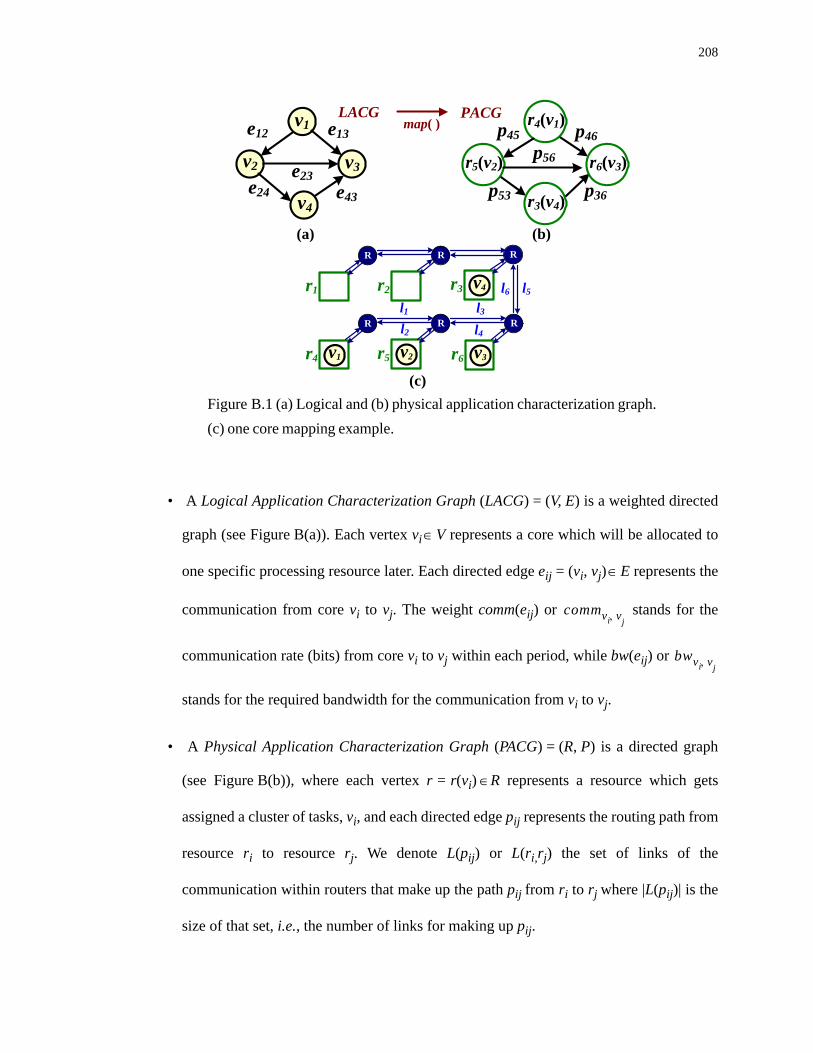
208

• A Logical Application Characterization Graph (LACG) = (V, E) is a weighted directed

graph (see Figure B(a)). Each vertex vi V represents a core which will be allocated to

one specific processing resource later. Each directed edge eij = (vi, vj) E represents the

communication from core vi to vj. The weight comm(eij) or stands for the

communication rate (bits) from core vi to vj within each period, while bw(eij) or

stands for the required bandwidth for the communication from vi to vj.

• A Physical Application Characterization Graph (PACG) = (R, P) is a directed graph

(see Figure B(b)), where each vertex r = r(vi) R represents a resource which gets

assigned a cluster of tasks, vi, and each directed edge pij represents the routing path from

resource ri to resource rj. We denote L(pij) or L(ri,rj) the set of links of the

communication within routers that make up the path pij from ri to rj where |L(pij)| is the

size of that set, i.e., the number of links for making up pij.

Figure B.1 (a) Logical and (b) physical application characterization graph.(c) one core mapping example.

(a) (b)

(c)

v1

v4

e13

e43

e12

v3v2

e24

r4(v1)p45

p53

p46

r5(v2) r6(v3)

r3(v4)

LACG PACGmap( )

p36

e23

p56

l1

l2

l3

R

l4R RR

l5l6

r6 v3r5 v2r4 v1

r3 v4

RR

r2r1

∈

∈

commvi v, j

bwvi v, j

∈

209

A mapping function map( ) maps the cores in the LACG to the resources in the NoC;

under a given routing mechanism, this results in the PACG.

Figure B(c) shows the mapping result of the LACG under the deterministic XY routing:

cores v1, v2, v3, and v4 are mapped onto resources r4, r5, r6, and r3, respectively, and

L(p45) = {l1}, L(p46) = {l1, l3}, L(p53) = {l3, l6}, L(p36) = {l5}, and L(p56) = {l3}. Note that as

defined the types of network contention in Section 6.3.1, source-based contention occurs in

this case since L(p45) L(p46) = {l1} , while the destination-based contention occurs

since L(p46) L(p56) = {l3} . And the path-based contention occurs since

L(p46) L(p53) = {l3} . With the motivation of significant impact on path-based

contention (see discussion in Figure 6.3), in what follows, we summarize our ILP-based

contention-aware mapping with path-based contention minimized.

B.3. Problem Formulation

Given the application characteristics and the NoC architecture, our objective is to map the

IP cores onto the NoC resources such that the sum of the weighted communication distance

and path-based network contention are minimized under a given routing mechanism. Of note,

minimizing the weighted communication distance directly contributes to minimizing the

communication energy consumption as well. More formally:

Given the LACG of the application, the routing mechanism, and the NoC architecture

Find a mapping function map( ) from LACG = (V, E) to PACG = (R, P) which minimizes:

min{ (B.1)

+ } for i k and j l

such that:

∩ ∅≠

∩ ∅≠

∩ ∅≠

1 α–( )β

----------------- comm eij( ) L map eij( )( )×[ ]eij∀ E∈∑×

αγ--- L map eij( )( ) L map ekl( )( )∩× ≠ ≠

210

(B.2)

(B.3)

(B.4)

where if and Bk is the capacity for link lk

Since the communication distance and path-based contention count have different units,

the normalization of these two metrics is approximated by assuming a worst-case scenario.

More precisely, β is set to ( ) × ( ) for an N × N NoC platform,

where the second factor, , is the longest distance in the network. γ is set to the

average number of path-based contentions of reasonable random mapping configurations. α is

a weighting coefficient meant to balance the communication distance and the contention

count. More precisely, we set α as the ratio of “the number of cores” to “the number of

resources + 1” (i.e., α = |V|/(|R| + 1)). If the number of cores is much smaller than the number

of resources (i.e., α is small), in order to avoid a higher communication distance, the first term

in (1) has a higher weight. Equation B.2 and Equation B.3 basically mean that each core

should be mapped to exactly one resource and no resource can host more than one core.

Finally, Equation B.4 guarantees that the load of each link will not exceed its bandwidth.

B.4. ILP-based Contention-aware Mapping Approach

B.4.1. Parameters and Variables

The given parameters are as follows:

• stands for the Manhattan Distance from resource rs to rt.

vi∀ V∈ , map vi( ) r vi( ) R∈=

vi∀ vj≠ V,∈ r vi( ) r vj( )≠

link lk∀ bwvi v, jlkmap vi( ) map vj( ),

Bk≤×vi vj,( )∀ E∈

∑,

lkmap vi( ) map vj( ),

1= lk L map vi( ) map vj( ),( )∈

comm eij( )eij∀ E∈∑ 2 N 1–( )×

2 N 1–( )×

MDrsrt

211

• The NoC architecture consists of |K| uni-directional segment links with IDs {l1, l2, ...,

l|K|}.

• For each link lk, where k = 1~|K|, represents whether or not this link lk is part of the

routing path from resource rs to resource rt, i.e., . Of note,

the above parameters are known under a given NoC architecture with a fixed routing

mechanism.

The variables of interest are as follows:

• shows the mapping result and can only take values in {0, 1}. More precisely, this

variable is set to 1, if the core vi is mapped onto resource rs.

• shows the communication path result and can only be {0, 1}. This variable is set to

1, if the communication path is made up from resources rs to rt, where cores vi and vj are

mapped onto.

• shows the path-based contention and can only be {0, 1}. This

variable is set to 1, while the cores vi, vj, vm, and vn are mapped onto resources rs, rt, rp,

and rq and at the same time, the communication path from resource rs to resource rt

shares the link lk with the path from resource rp to resource rq.

B.4.2. Objective Function

Our objective is to minimize the weighted communication distance and the path-based

network contentions as well, i.e.,

lkrsrt

lkrsrt 1 if lk L rs rt,( )∈,

0 otherwise ,⎩⎨⎧

=

mvi

rs

pvivj

rsrt

zlk_ vivjvmvnrsrtrprq( )

212

{

} (B.5)

B.4.3. Constraints

The following constraints are used:

• One-to-one core-to-resource mapping: Each resource cannot accept more than one core

(see Equation B.6). Each core should be mapped onto a specific resource (see Equation

B.7). Equation B.8 makes sure that variables are set to be either 0 or 1.

(B.6)

(B.7)

(B.8)

• Communication path: Any two communicating cores that belong to two different

resources make up a path. Therefore,

(B.9)

To transform Equation B.9 into an ILP formulation, we impose the following constraints:

(B.10)

(B.11)

• Bandwidth constraint on each link: For each k, all possible paths through link lk cannot

exceed its bandwidth Bk.

1 α–( )β

----------------- commvi vj, MDrsrtpvivj

rsrt×r∀ s rt, R∈

∑⎝ ⎠⎜ ⎟⎛ ⎞

×vi vj,( )∀ E∈

∑×

αγ--- zlk_ vivjvmvnrsrtrprq( )

lk∀vi vj,( )∀ vm vn,( ), E∈

rs∀ rt rp rq, , , R∈

∑×+

mvi

rs

rs∀ R∈ mvi

rs 1≤vi∀ V∈∑,

vi∀ V∈ mvi

rs

rs∀ R∈∑, 1=

vi V rs R∈,∈∀ 0 m≤ vi

rs, 1≤

vi vj,( )∀ E∈ pvivj

rsrt 1 if mvi

rs 1=⎝ ⎠⎛ ⎞ and mvj

rt 1=⎝ ⎠⎛ ⎞,

0 otherwise ,⎩⎪⎨⎪⎧

=,

mvi

rs mvj

rt 1–+ pvivj

rsrtmvi

rs mvj

rt+

2----------------------≤ ≤

0 p≤ vivj

rsrt 1≤

213

(B.12)

• Path-based network contention count: This type of contention occurs when two paths

with different sources or different destinations contend for the same link. Therefore,

(B.13)

if (B.14)

To transform Equation B.14 into an ILP formulation, we impose the following constraints:

(B.15)

(B.16)

Equation B.15 and Equation B.16 determine whether or not the path-based contention

occurs; if so, this variable is set to be 1.

B.5. Experimental Results

B.5.1. Experiments using Synthetic Applications

We first evaluate the number of path-based contentions on application mapping for a 4 × 4

NoC platform under three different scenarios: random (or adhoc) mapping, energy-aware

mapping [79] and our contention-aware mapping. Several sets of synthetic applications are

generated using the TGFF package [162]. The number of cores used in this experiment ranges

from 12 to 16, while the number of edges varies from 15, 20, ..., to 60 (organized in 10

categories). For each category, we generate 100 random task graphs and the corresponding

bwvi v, jlkrsrt× pvivj

rsrt Bk≤×vi vj,( )∀ E∈

∑rs∀ rt, R∈

∑

lkrsrt∀ L rs rt,( )∈⎝ ⎠

⎛ ⎞ & lkrprq∀ L rp rq,( )∈⎝ ⎠

⎛ ⎞

vi vj,( )∀ vm vn,( ), E∈i m & j n≠ ≠

rs∀ rt rp rq, , , R∈

zlk_ vivjvmvnrsrtrprq( ) 1= mvi

rs mvj

rt mvm

rp mvn

rq 1= = = =

pvivj

rsrt pvmvn

rprq lkrsrt lk

rprq 3–+ + + zlk_ vivjvmvnrsrtrprq( )≤

0 z≤ lk_ vivjvmvnrsrtrprq( ) 1≤

214

results (i.e., number of contentions, communication energy consumption, system throughput)

are calculated.

Figure B.2 shows the number of path-based contentions comparing these three scenarios,

while Table B.1 shows the communication energy ratio and throughput savings normalized to

the results of energy-aware mapping approach in [79] and contention-aware mapping

approaches for the selected categories (the number of edges set to 20, 30, 40, and 50). Of note,

The communication energy consumption and the packet latency are measured by a C++

simulator using the bit energy model in [170].

Table B.1 Energy and throughput comparison between energy-aware in [79] and contention-aware mapping.

As we can see in Figure B.2, the contention-aware mapping effectively reduces the path-

based contention. Moreover, the reduction increases as the number of edges scales up. For

instance, for task graphs with 50 edges, the number of path-based contention in the mapping

configuration can be reduced from 36 to 5. As observed in Table B.1, under the contention-

# of edges 20 30 40 50communication energy ratio 1.02 1.07 1.11 1.08

throughput savings 18.2% 24.1% 21.8% 13.5%

15 20 25 30 35 40 45 50 55 600

20

40

60random mappingenergy-aware mappingcontention-aware mapping

Figure B.2 Path-based contention count in a 4 × 4 NoC comparing therandom, energy-aware in [79] and contention-aware mapping.

# of edges in the task graph

cont

entio

n#

of p

ath-

base

d

215

aware mapping, the communication energy consumption is up to 11%1 larger compared to the

energy-aware mapping solution; however, the system throughput can be improved around

19.4%, on average. From Figure B.2 and Table B.1, it can be concluded that the contention-

aware mapping effectively reduces the path-based contention which achieves great system

throughput improvement with negligible energy loss.

B.5.2. Experiments using Real Applications

To evaluate the potential of our contention-aware idea for real-time examples, we apply it to

several benchmarks, such as examples with high degree of parallelism (Parallel-1 and Parallel-

2) [143], LU Decomposition [143], and MPEG4 decoder [159]. In Table B.2, the first three

benchmarks are mapped onto a 3 × 3 NoC platform, while the last is onto a 4 × 4 NoC platform.

The first through the fifth columns in Table B.2 show, respectively, the name of the benchmark,

the number of cores and edges in the LACG, the communication energy loss and the throughput

savings of our contention-aware solution compared to the energy-aware solution [79].

As seen in Table B.2, our contention-aware solution can achieve 17.4% throughput

savings, on average, with the communication energy loss within 9% compared to energy-

aware solution in [79].

Table B.2 Communication energy overhead and throughput improvement of our contention-aware solution compared to the energy-aware solution [79].

1. We note that this is only the communication energy part. If the communication energy consumptionis around 20% of the total energy consumption (as shown in [94]), we have only 2.2% energy loss.

benchmarks cores edgescomm. energy

overheadthroughput

improvementParallel-1 9 13 0% 16.9%Parallel-2 9 15 8.8% 20.4%

LU Decomposition 9 11 6.5% 14.1%MPEG4 Decoder 12 26 3.6% 18.2%

216

Figure B.3 plots the LACG of the Parallel-1 benchmark (see Figure B.3(a)), the mapping

results under two scenarios: energy-aware mapping [79] using ILP approach and our

contention-aware mapping approach (see Figure B.3(b) and (c), respectively), while the

average packet latency comparison for different injection rates in these two scenarios (see

Figure B.3(d)). The existing path-based contentions are highlighted in the mapping results. As

seen the energy-aware mapping result in Figure B.3(b), there are two pairs of path-based

contention in the network, while no path-based contention occurs when using the contention-

aware approach. We observe that for such path-based contention, the average latency goes up

dramatically after the packet injection rate exceeds a critical point (i.e. the network gets into

the congestion mode, see Figure B.3(d)). Also, when contention-aware constraints are taken

into consideration during the mapping process, the throughput for Parallel-1 moves from

0.2173 (packet/cycle) to 0.254 which represents about 16.9% throughput improvement.

0.1 0.15 0.2 0.25 0.30

100

200

300

400 energy-aware mapping [5]contention-aware mapping

12

3

46 8

7 9

5 12

3

468

7 9

5

1

2 3 4

6

87

9

5

Figure B.3 (a) Parallel-1 benchmark (b)(c) Mapping results of the energy-aware approach [79] and our contention-aware method (d) Average packetlatency and throughput comparison under these two mapping methods.

avg.

pac

ket l

aten

cy

Parallel-1

path-based contention


(a) (b) (c)

(d)

217

B.6. Summary

In this appendix, we have addressed the issue of off-line core-resource mapping for NoC-

based platforms while considering the critical network contention minimization. We have

reported our results obtained from many experiments involving both synthetic and real

benchmarks. Experimental results show that, compared to other existing mapping approaches

based on communication energy minimization, our contention-aware mapping technique (with

the goal of reducing the path-based network contention) achieves a significant decrease in

packet latency (and implicitly, a throughput increase) with a negligible communication energy

overhead.

Although in this appendix we focus on 2-D mesh NoCs with XY routing, our idea can be

further adapted to other architectures implementing under different network topologies with

deterministic routing schemes. Moreover, the idea of minimizing the network contention is

not limited to core-resource mapping as presented. Instead, it can be applied to other NoC

synthesis problems and the mapping/scheduling heuristics on parallel systems to achieve

further system throughput improvements.

Designing Embedded Multiprocessor Networks-on-Chip - CiteSeerX

Documents

Transcript of Designing Embedded Multiprocessor Networks-on-Chip - CiteSeerX