Designing a Frequency Selective Scheduler for WiMAX using ...
77
Designing a Frequency Selective Scheduler for WiMAX using Genetic Algorithms University of Stuttgart Institute of Communication Networks and Computer Engineering Prof. Dr.-Ing. Dr. h. c. mult. Paul J. Kühn Marc Necker, Mathias Kaschub, Elias Doumith Miquel Testar Quer 1 st August 2008
Transcript of Designing a Frequency Selective Scheduler for WiMAX using ...

Designing a Frequency Selective Scheduler for WiMAX using
Genetic Algorithms
University of Stuttgart
Institute of Communication Networks and Computer Engineering Prof. Dr.-Ing. Dr. h. c. mult. Paul J. Kühn
Marc Necker, Mathias Kaschub, Elias Doumith
Miquel Testar Quer 1st August 2008

ii

Contents
1 Introduction 11.1 Motivation . . . . . . . . . . . . . . . . . . . . . . . . . . . . . . . . . . . . . . . 11.2 Wireless communications environment . . . . . . . . . . . . . . . . . . . . . . . . 1
1.2.1 Multipath propagation . . . . . . . . . . . . . . . . . . . . . . . . . . . . . 21.2.2 Parameters of a wireless communications environment . . . . . . . . . . . 2
I Background information 5
2 WiMAX (IEEE 802.16) 72.1 Historic context . . . . . . . . . . . . . . . . . . . . . . . . . . . . . . . . . . . . . 72.2 Physical layer . . . . . . . . . . . . . . . . . . . . . . . . . . . . . . . . . . . . . . 8
2.2.1 OFDM . . . . . . . . . . . . . . . . . . . . . . . . . . . . . . . . . . . . . 82.2.2 Channel coding . . . . . . . . . . . . . . . . . . . . . . . . . . . . . . . . . 102.2.3 Symbol structure . . . . . . . . . . . . . . . . . . . . . . . . . . . . . . . . 112.2.4 Subchannel and subcarrier permutation . . . . . . . . . . . . . . . . . . . 12
2.3 MAC layer . . . . . . . . . . . . . . . . . . . . . . . . . . . . . . . . . . . . . . . 142.3.1 MAC PDU . . . . . . . . . . . . . . . . . . . . . . . . . . . . . . . . . . . 142.3.2 ARQ . . . . . . . . . . . . . . . . . . . . . . . . . . . . . . . . . . . . . . . 142.3.3 Quality of service . . . . . . . . . . . . . . . . . . . . . . . . . . . . . . . . 15
2.4 Frame structure . . . . . . . . . . . . . . . . . . . . . . . . . . . . . . . . . . . . . 15
3 Packing problems 173.1 Overview . . . . . . . . . . . . . . . . . . . . . . . . . . . . . . . . . . . . . . . . 173.2 Bin packing problems . . . . . . . . . . . . . . . . . . . . . . . . . . . . . . . . . 17
3.2.1 Solving . . . . . . . . . . . . . . . . . . . . . . . . . . . . . . . . . . . . . 173.3 Knapsack problems . . . . . . . . . . . . . . . . . . . . . . . . . . . . . . . . . . . 18
3.3.1 Solving . . . . . . . . . . . . . . . . . . . . . . . . . . . . . . . . . . . . . 19
4 Evolutionary algorithms 214.1 Overview of evolutionary algorithms . . . . . . . . . . . . . . . . . . . . . . . . . 214.2 Genetic algorithms . . . . . . . . . . . . . . . . . . . . . . . . . . . . . . . . . . . 22
4.2.1 Representation of the solutions . . . . . . . . . . . . . . . . . . . . . . . . 224.2.2 Evolution strategies . . . . . . . . . . . . . . . . . . . . . . . . . . . . . . 234.2.3 Genetic operators . . . . . . . . . . . . . . . . . . . . . . . . . . . . . . . . 244.2.4 Selection . . . . . . . . . . . . . . . . . . . . . . . . . . . . . . . . . . . . 254.2.5 Termination Criteria . . . . . . . . . . . . . . . . . . . . . . . . . . . . . . 26
II Design and simulation 27
5 Description of the problem 29
6 Problem modelling 316.1 Non-selective approach . . . . . . . . . . . . . . . . . . . . . . . . . . . . . . . . . 31
iii

Contents
6.1.1 Common resource . . . . . . . . . . . . . . . . . . . . . . . . . . . . . . . 316.1.2 Users . . . . . . . . . . . . . . . . . . . . . . . . . . . . . . . . . . . . . . 316.1.3 Representation of the solutions . . . . . . . . . . . . . . . . . . . . . . . . 316.1.4 Initialization . . . . . . . . . . . . . . . . . . . . . . . . . . . . . . . . . . 316.1.5 Genetic algorithm . . . . . . . . . . . . . . . . . . . . . . . . . . . . . . . 326.1.6 Genetic operators . . . . . . . . . . . . . . . . . . . . . . . . . . . . . . . . 326.1.7 Placement algorithm . . . . . . . . . . . . . . . . . . . . . . . . . . . . . . 32
6.2 Frequency selective approach . . . . . . . . . . . . . . . . . . . . . . . . . . . . . 336.2.1 Common resource . . . . . . . . . . . . . . . . . . . . . . . . . . . . . . . 336.2.2 Users . . . . . . . . . . . . . . . . . . . . . . . . . . . . . . . . . . . . . . 336.2.3 Placement algorithm . . . . . . . . . . . . . . . . . . . . . . . . . . . . . . 346.2.4 Representation of the solution . . . . . . . . . . . . . . . . . . . . . . . . . 366.2.5 Initialization . . . . . . . . . . . . . . . . . . . . . . . . . . . . . . . . . . 376.2.6 Genetic algorithm . . . . . . . . . . . . . . . . . . . . . . . . . . . . . . . 376.2.7 Genetic operators . . . . . . . . . . . . . . . . . . . . . . . . . . . . . . . . 376.2.8 Parameters of the simulation . . . . . . . . . . . . . . . . . . . . . . . . . 38
6.3 Implementation . . . . . . . . . . . . . . . . . . . . . . . . . . . . . . . . . . . . . 396.3.1 Program structure . . . . . . . . . . . . . . . . . . . . . . . . . . . . . . . 396.3.2 Libraries used . . . . . . . . . . . . . . . . . . . . . . . . . . . . . . . . . . 41
7 Results of the simulation 457.1 Genetic operators . . . . . . . . . . . . . . . . . . . . . . . . . . . . . . . . . . . . 46
7.1.1 Swap, change and S&C . . . . . . . . . . . . . . . . . . . . . . . . . . . . 467.1.2 S&C II . . . . . . . . . . . . . . . . . . . . . . . . . . . . . . . . . . . . . 477.1.3 Normal distributed change mutator . . . . . . . . . . . . . . . . . . . . . . 47
7.2 Parameter evaluation . . . . . . . . . . . . . . . . . . . . . . . . . . . . . . . . . . 487.2.1 Crossover parameter effect . . . . . . . . . . . . . . . . . . . . . . . . . . . 497.2.2 Population size and number of generations . . . . . . . . . . . . . . . . . 49
7.3 Deterministic crowding . . . . . . . . . . . . . . . . . . . . . . . . . . . . . . . . . 517.4 Different scenarios . . . . . . . . . . . . . . . . . . . . . . . . . . . . . . . . . . . 51
8 Conclusion and outlook 538.1 Conclusion . . . . . . . . . . . . . . . . . . . . . . . . . . . . . . . . . . . . . . . 538.2 Outlook . . . . . . . . . . . . . . . . . . . . . . . . . . . . . . . . . . . . . . . . . 54
A Selective simulation 55A.1 Startup phase . . . . . . . . . . . . . . . . . . . . . . . . . . . . . . . . . . . . . . 55A.2 Placement phase . . . . . . . . . . . . . . . . . . . . . . . . . . . . . . . . . . . . 56
B BLER tables 59
C List of figures 63
D References 67
E Appreciations 71
F Author’s Statement 73
iv
1 Introduction
1.1 Motivation
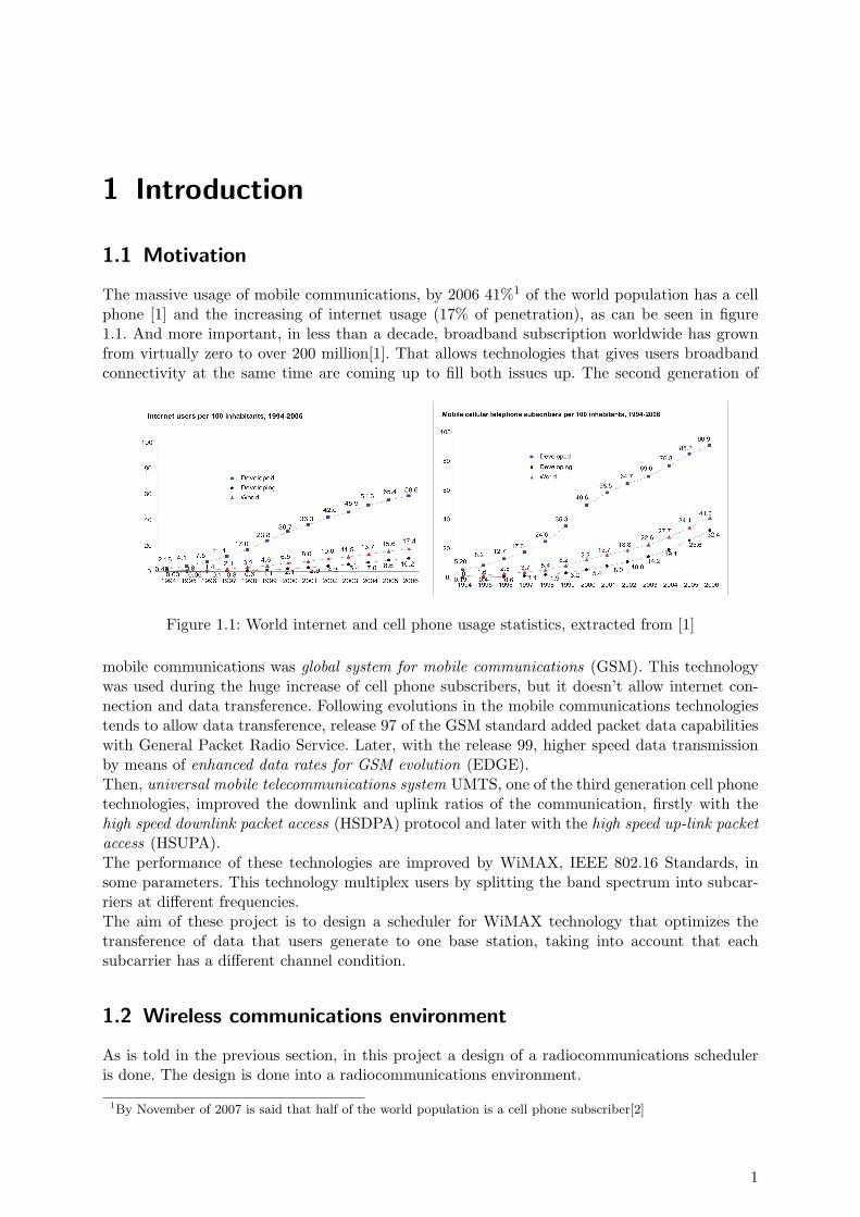
The massive usage of mobile communications, by 2006 41%1 of the world population has a cellphone [1] and the increasing of internet usage (17% of penetration), as can be seen in figure1.1. And more important, in less than a decade, broadband subscription worldwide has grownfrom virtually zero to over 200 million[1]. That allows technologies that gives users broadbandconnectivity at the same time are coming up to fill both issues up. The second generation of
Figure 1.1: World internet and cell phone usage statistics, extracted from [1]
mobile communications was global system for mobile communications (GSM). This technologywas used during the huge increase of cell phone subscribers, but it doesn’t allow internet con-nection and data transference. Following evolutions in the mobile communications technologiestends to allow data transference, release 97 of the GSM standard added packet data capabilitieswith General Packet Radio Service. Later, with the release 99, higher speed data transmissionby means of enhanced data rates for GSM evolution (EDGE).Then, universal mobile telecommunications system UMTS, one of the third generation cell phonetechnologies, improved the downlink and uplink ratios of the communication, firstly with thehigh speed downlink packet access (HSDPA) protocol and later with the high speed up-link packetaccess (HSUPA).The performance of these technologies are improved by WiMAX, IEEE 802.16 Standards, insome parameters. This technology multiplex users by splitting the band spectrum into subcar-riers at different frequencies.The aim of these project is to design a scheduler for WiMAX technology that optimizes thetransference of data that users generate to one base station, taking into account that eachsubcarrier has a different channel condition.
1.2 Wireless communications environment
As is told in the previous section, in this project a design of a radiocommunications scheduleris done. The design is done into a radiocommunications environment.
1By November of 2007 is said that half of the world population is a cell phone subscriber[2]
1

1 Introduction
A radiocommunications environment is characterized by a base station and multiple mobilestations in a cell.
• The cell is the portion of space that is served by one base station.
• The base station sends and receive data from all the mobile stations in a cell
• The mobile station is each one of the user equipments that sends its requests and receivethe answers
1.2.1 Multipath propagation
Inside the cell, there can be obstacles. These obstacles makes transmissions between base andmobile stations not ideal. That’s because these obstacles creates different paths between thebase and one mobile station, this is the multipath propagation.The multipath propagation means that a station will receive multiple copies of the same signal,but with differences in some parameters of the signal. These parameters are:
• Phase
• Time delay
• Power
Figure 1.2: Multipath propagation, extracted from [3]
h(τ, t) =∑k
Ak(t)δ(τ − τk(t)) (1.1)
More details over multipath propagation can be consulted in [3].
1.2.2 Parameters of a wireless communications environment
The performance of the communications channel is modeled by taking into account the followingparameters.
2

1.2 Wireless communications environment
Figure 1.3: Effect of multiple signal arrivals with various delays
Delay spread
A mobile station receives various copies of the signal with different delays, see figure 1.2. Themaximum time interval while the station receives signal with significant energy is the delayspread, so the difference between the LOS signal and last component.The delay spread depends mainly on the terrain type, the environment (urban, suburban,rural). In urban environments this value can be around 10 µs, for further information consult [4].
Bc =1
2πDs(1.2)
Directly derived from the delay spread is the coherence bandwidth. In the equation 1.2 Bc isthe coherence bandwidth and Ds is the delay spread. The coherence bandwidth is the band overwhich the channel transfer function remains virtually constant. So the criterion is satisfied ifthe transmission bandwidth does not exceed the coherence bandwidth of the channel. There-fore, if the transmission bandwidth doesn’t exceed the coherence bandwidth of the channel, thetransmission doesn’t suffer distorsion.
Fading
In both directions, from base station to mobile station and vice-versa, as can be seen in figure1.3, signal is received with variations of the presented before parameters. And this createsfading2. We have two types of fading; fast fading and slow fading.
• Slow fading is caused when shadowing occurs. The duration of the fading depends onthe time that the mobile needs to be ahead of the shadow created by the obstacle. Thisvariation follows a lognormal probability density function.
• Fast fading is caused directly by the multipath effect. Receiving the signals with delaysthat are fractions of λ, makes drastic change in the sum of the different signals, we canhave constructive or destructive sums.In fact, there are two types of fast fading; it depends on how far is the echo created. Ifit’s a nearly created echo, the delay between two signals is small related to the time ofthe symbol, there’s a constructive or destructive sum, but there’s not dispersion3. On theother hand, when the echo is further created, the delay between two signals is big relatedto the time of the symbol, there’s dispersion.
2Fading refers to the distortion that a carrier-modulated telecommunication signal experiences over certainpropagation media
3Is said that a channel is dispersive, when the module of transfer function is not constant and the phase is notlinear
3

1 Introduction
Path loss
The reduction in power density of an electormagnetic wave as it propagates is called path loss(or attenuation).Path loss is produced by many effects like free-space loss, refraction, diffraction, reflection, differ-ence between theoretical and practical antenna gain and absorption. Therefore, it’s influenced bydistance from the transmitter to the receiver, location of the antennas, terrain type, environmentand weather.
L = 10n log10(d) (1.3)
In the equation L is the path loss in dB, d is the distance between transmitter and receiver andn is the path loss exponent. The path loss exponent is a way to represent the path loss.The value of the path loss exponent is from 2 to 4 outdoors. 2 is the value when propagationoccurs in free space and 4 when it occurs in an environment with huge density of obstacles(urban). Indoors, the exponent varies from 4 to 6. But the calculation of the delay spread is,in fact, a prediction. An exact prediction is not allways possible, only for the simplest like freespace propagation. For other cases empirical methods are used, these are based on averagedlosses along typical radio links. Most commonly used methods are Okumura-Hata or COST-231(Okumura-Hata extension). Hata model has three varieties of equation for urban, suburban andrural environments, and to calculate the path loss takes into account: distance, heights of theantennas and frequency of the transmission.
4

Part I
Background information
5


2 WiMAX (IEEE 802.16)
The technology which this thesis is based on is WiMAX, this chapter pretends to introduce intothe key features of this technology that will be used to to face the scheduling problem.
2.1 Historic context
In this section WiMAX is located in its context into the broadband wireless communicationshistory.
Broadband wireless
The history of broadband wireless remains in the desire of finding an alternative to wired accesstechnologies.Firstly, applications were oriented to cover voice telephony demand and were called wirelesslocal-loop (WLL). These were successfull in countries with a developing economy, because theexisting local loop infrastructure was not enable to serve the increasing demand. But in marketsthat had already good scaled local-loop infrastructure for voice telephony, WLL began to havesense with the start of the commercialization of Internet, in 1993.Then with the tendency to broadband and thanks to digital subscriber line DSL1 and cable,
Figure 2.1: LOS and NLOS
wireless systems evolved to support higher speeds. In this way line of sight (LOS), see figure2.1, systems were developed. Two type of systems were designed:
• Local multipoint distribution systems (LMDS) achieved high speed, working in the mil-limeter band (24 or 39 GHz). Its services were mainly targeted at business users and hatsuccess in the late 1990’s. But LOS requirements, involved installing antennas in rooftops,moreover the short range of the technology; stop the growth of this technology, by changingto other ones.
• Multichannel multipoint distribution service (MMDS), with a band between 2 and 3 GHz.This technology was mainly used to provide TV broadcasting in not cabled zones. In this
1DSL is a family of technologies that provide digital data transmission over the wires of a local telephone network
7

2 WiMAX (IEEE 802.16)
case the growth of satellite TV induced to a redefinition of the target, and the systemwas used to serve Internet access. Instead the coverage could be quite large, using tallbase station antennas and high power transmitters, the capacity was too limited. This factand the LOS requirements became on the main impediments to the higher success of thistechnology.
The next generation of broadband wireless systems overcome the LOS problem. This was doneby tending to a cellular architecture and implementing a better signal processing techniques,these are non line of sight NLOS applications, more information can be found in [5]
WiMAX
With the aim of finding a interoperable solution for the emerging wireless broadband, the In-stitute of Electronic and Electrical Engineers (IEEE) created the 802.16 group. It was initiallyfocused on developing a LOS broadband system, to operate in the 10 GHz to 66 GHz band.The standard developed, completed in December 2001, was based on a single carrier and timemultiplexed (TDM)2.The next step was the 802.16a amendment that includes NLOS applications, working on the 2GHz to 11 GHz band, and uses orthogonal frequency division multiplex technology (OFDM)3
and OFDMA.These revisions of the standard followed with the IEEE 802.16-2004 that replaced prior versionsand focused on the fixed applications. One year later, the IEEE 802.16-2005 targeted on mobileapplications, and called mobile WiMAX.[11]
2.2 Physical layer
The physical layer is the first of the seven layer OSI model. The physical layer provides anelectrical and mechanical interface to the transmission medium.As was said the WiMAX physical layer is based on OFDM and it’s going to be presented insection 2.2.1. Further information that what are going to be presented in this section can beconsulted in [5], [6], [8], [10] and [7].
2.2.1 OFDM
This technology is used in multiple types of communications. In wired communications; DSL,power line communications PLC4 and in wireless communication; wireless LAN (802.11), terres-trial digital system digital video broadcasting terrestrial (DVB-T) or digital video broadcasting -handheld (DVB-H) amongst others. OFDM is a multicarrier modulation scheme utilized as adigital multicarrier modulation method. It’s based on dividing a given high-rate data streaminto several parallel smaller data streams or channel, and modulate each stream on separatecarriers, called subcarriers.
The term orthogonal in OFDM refers to the fact that subcarriers are perfectly separable overthe symbol duration. To ensure orthogonality; the frequency of the first subcarrier such thathas an integer number of cycles during a symbol period has to be chosen. Also a space betweensubcarriers such that BISc = B
Nsc, where B is the total assigned bandwidth and Nsc is the
number of subcarriers, has to be taken. This structure is quite easy to implement by directly
2With time multiplexing, all the users in a cell are using the same band, the resource is divide by giving eachuser a concrete time slot to transmit
3This technology uses time and frequency multiplexing at the same time. It will be deeply explain in subsec-tion 2.2.1
4PLC is a system for carrying data on a conductor also used for electric power transmission
8

2.2 Physical layer
doing IFFT5 and FFT in transmission and reception, respectively.
Multicarrier modulation minimize intersymbol interference (ISI)6. Splitting data stream intomany parallel streams increases the symbol duration and makes symbol’s time large enoughover the delay spread of the channel. Ts
L � τ , where Ts is the time of symbol, L is the numberof streams and τ is the delay spread.
In order to keep each OFDM symbol independent among others over the channel, is necessaryto introduce a guard time between symbols, introducing a larger guard band is possible toguarantee that there’s no interference between OFDM symbols, further information can beconsulted in [5] and [6].
A key feature of the OFDM is the synchronization in both dimensions:
• Timing synchronization: The margin of desychronization achievable is the difference be-tween the delay spread and the duration of the cyclic prefix, 0 ≤ τ ≤ (Tm−Tg). Where Tmis the maximum delay spread, Tg is the duration of the cyclic prefix and τ is the allowederror in synchronization.
• Frequency synchronization: This type of synchronization is not as relaxed as the timing,because the orthogonality of the data symbols is centered on their perceptible in thefrequency domain. A small offset produces, intercarrier interference (ICI).
Advantages of OFDM
• Reduced computational complexity: OFDM can be implemented using fast Fourier trans-form (FFT) and inverse Fourier transform (IFFT).
• Slow degradation of performance under delay spread: Performance of an OFDM systemdegrades slowly as the delay spread grows over the maximum delay spread which wasdesigned for optimal performance.
• Exploitation of frequency diversity: OFDM facilitates coding and interleaving subcarriersin the frequency domain, which provide robustness against burst errors, parts of the datathat are transmitted into spectral bad channel conditions.
• Use as a multiaccess scheme: OFDM is also used as a multiaccess scheme, where theresource are partitioned among other users. This is called Orthogonal frequency multipleaccess OFDMA and is used in Mobile WiMAX.
Despite these, OFDM also have some problems. When there’s a high peak to average power ratio(PAPR). OFDM have a higher PAPR than single carriers. That’s because in the time domain, amulticarrier signal is the sum of the narrowband signals; this sum is very variable over the time,so the peak value of the signal is quite larger than the average. This fact brings to nonlinearitiesand clipping distortion7. It becomes a tradeoff between a reduction of efficiency and an increaseof the cost of the RF power amplifier.
OFDMA
Orthogonal frequency division multiple access is a multiple access method based on OFDM thatallows simultaneous transmissions to/from several users along with advantages of OFDM. It’s
5FFT and IFFT are a relatively low computational load algorithms to compute the discrete Fourier transformand its inverse
6ISI is a form of distortion of a signal in which one symbol interferes with subsequent symbols7Clipping distortion occurs when the receiver can’t trace the signal, because its amplitude goes over the bounds
that the receiver is able to manage
9

2 WiMAX (IEEE 802.16)
Parameters ValuesSystem channel bandwidth (MHz) 1.25 5 10 20
FFT size (NFFT ) 128 512 1024 2048Subcarrier frequency spacing 10.94 kHz
Useful symbol time (Tb = 1/f) 91.4 µsGuard time (Tg = Tb/8) 11.4 µs
OFDMA symbol duration (Ts = Tb + Tg) 102.9 µs
Table 2.1: OFDMA scalability parameters
essentially frequency division multiple access FDMA and time division multiple access TDMA atthe same time. Users are dynamically assigned to subcarriers, like FDMA, in different time slots,like TDMA. While in fixed WiMAX, OFDM with 256 subcarriers is used; OFDMA permits abetter mobile usage. Subcarriers are assigned to subchannels that can be allocated to differentusers, in this way high granularity from the spectrum point of view can be achieved, and permitsvarious approaches on the subcarrier permutation as will be explained in subsection 2.2.4that improves performances versus interference of other cells. Another advantage of OFDMArelative to OFDM is that manages better the PAPR problem. That’s because when splitting thebandwidth among all the mobile stations of the cell, makes that one MS only manages a subsetof the subcarriers, therefore each user transmits with smaller PAPR.
Scalable OFDMA
The design of OFDMA wireless systems deals with the choice of the number of subcarriers perchannel bandwidth. This election is always a tradeoff between protection against multipath,Doppler shift and design complexity.Increase the number of subcarriers means a better immunity to multipath propagation and ISIwill be achieved. But on the other hand it means the complexity, and cost, of the system and alsoleads to a narrower subcarrier spacing. And this makes the system more sensitive to Dopplershift and phase noise.In order to keep a suitable subcarrier spacing, in OFDMA, the FFT size is scaled by adjustingthe FFT size while fixing the sub-carrier frequency spacing at 10.94 kHz. The unit sub-carrierbandwidth and symbol duration is fixed, so the impact on higher layers is minimal when scalingthe bandwidth, parameters that can be seen in table 2.1. It has to be said that in order toreduce complexity, the profile was limited to FFT sizes of 512 and 1024.
2.2.2 Channel coding
Channel coding in WiMAX is based on FEC.Forward error correction (FEC) is an control system for errors in data transmission, where thesender adds redundant data to its messages. This allows the receiver to detect and correct errorswithout asking more data to be sent. More information than it’s going to be presented in thischapter can be consulted in [5] and [7].Data is divided into FEC blocks, and these blocks are placed into an entire number of subchan-nels8.The mandatory channel coding scheme in mobile WiMAX is based on binary nonrecursive con-volutional coding.Mobile WiMAX permits various types of coding to correct data; convolutional coding (CC), con-volutional turbo code (CTC), block turbo code (BTC) and low density parity check code (LDPC),
8Subchannel are the granularity in the time/frequency resource
10

2.2 Physical layer
but the WiMAX Forum profile[12] only defines as mandatory CC and CTC.
Convolutional coding
In convolutional coding, a symbol of m length is converted to a n length symbol, where m/n isthe code rate and (m ≥ n). The transformation is a function of the last k information symbols,where k is the constraint length of the code, there are k memory registers, each holding oneinput bit. All memory registers start with a 0. Bits enter from the first register on the left sideand using the existing values in the remaining registers the output gets n bits, then all registervalues are shifted to the right and the next bit is expected. When there are not more bits goingin, the encoder output continues until all registers returns to zero state.CTC in WiMAX uses duo binary turbo codes. In duo binary turbo codes the encoder sends three
Figure 2.2: Recursive convolutional code scheme with 1/2 rate and constraint length 4
sub-blocks of bits. The first sub-block is the m-bit block of payload data, the second sub-blockis n/2 parity bits for the payload data, computed using a recursive systematic convolutionalcode (RSC code), the third sub-block is n/2 parity bits for a known permutation of the payloaddata, again computed using an RSC convolutional code. That’s, two redundant but differentsub-blocks of parity bits for the sent payload. The complete block has m+n bits of data witha code rate of m
(m+n) . The permutation of the payload data is carried out by a device calledinterleaver.
Interleaving
Interleaving is used in digital data transmission technology to protect the transmission againstburst errors. These errors overwrite a lot of bits in a row, and an error correction schemeexpects errors to be more uniformly distribute. Therefore interleaving is used to overcome thisfrom happening.The encoded bits are interleaved by two steps and is done independently on each FEC block.Firstly adjacent coded bits are not mapped on adjacent subcarriers (more frequency diversityis achieved), and then is ensured that adjacent bits are alternately mapped to less and moresignificant bits of the modulation constellation.
2.2.3 Symbol structure
During the symbol mapping stage, the sequence of binary bits is converted to a sequence ofcomplex valued symbols.
11

2 WiMAX (IEEE 802.16)
Mandatory constellations in WiMAX are QPSK and 16 QAM (see figure 2.3), 64 QAM is alsodefined in the standard as optional to transmit data, and BPSK can be used for broadcastcontrol messages. Then, the constellation used, the coding type and rate, together, are theburst profile.
Figure 2.3: QPSK and 16QAM constellation
Each modulation is scaled by a constant, because the average transmitted power is unity.As we commented in section 2.2.1, a data rate sequence of symbols is split into multiple parallellow data rate sequences, each of which is used to modulate an orthogonal subcarrier.In the frequency domain each OFDM symbol is created by mapping the sequence of symbols.WiMAX has three classes of subcarriers, distribution can be seen in 2.2.4:
• Data subcarriers are used for carrying data symbols.
• Pilot subcarriers that transmit pilot symbols, which are known a priory and are used toestimate the channel.
• Null subcarriers have no power allocated and are used to save the guard subcarriers, thisreduce the interference between adjacent channels.
Further information about the symbol structure can be obtained in [5].
Figure 2.4: OFDMA sub-carrier structure, extracted from [10]
2.2.4 Subchannel and subcarrier permutation
To create the OFDM symbol in the frequency domain, the modulated symbols are mapped onto the subchannels to transmit the data block.
12

2.2 Physical layer
In WiMAX subcarriers can be continuously mapped, one adjacent to the next one, or distributedthrough the whole band. When distributing subcarriers through the whole band, OFDMA sym-bols are transmitted at the same time in different regions of the band. Therefore, there aresubcarriers that have an SINR over the mean and others that are under the mean, so there’s anaveraging of the channel. In this way frequency diversity is ensured.The other option is to map the subcarriers continuously. In this way, whole OFDMA symbolsare transmitted in the same region of the band, there’s no averaging of the channel, then somesymbols has a better SINR than others. With this approach the system can take advantage ofthe fluctuations of the channel. The idea is transmit as high a data rate is possible when thechannel is good and reduce the rate when the channel is poor, by using smaller constellations,to avoid an increase of packets dropped.
Full usage of subcarriers
In full usage of subcarriers (FUSC), all data subcarriers are used. Each subchannel is madeup of 48 data subcarriers, which are randomly distributed through the whole frequency band.Pilot subcarriers are first allocated and the remaining subcarriers are permutated on the varioussubchannels. That allows to average the channel response for all symbols.
Partial usage of subcarriers
The difference between partial usage of subcarriers PUSC and FUSC, is that PUSC subcarriersare firstly divided into six groups. Then, permutation of subcarriers to create subchannels isdone separately for each group.All subcarriers except the null ones are arranged in clusters, each cluster consists of 14 adjacentsubcarriers over two OFDM symbols. Inside the clusters; 24 subcarriers are used to transmitdata and 4 are pilot subcarriers. The clusters are then renumbered, which makes a redistributionof the clusters.Once clusters are renumbered, six groups are made taking a part of the total number of clusters,and a subchannel is the union of two clusters of the same group.With PUSC is possible to assign a set of the group of carriers to a base station, by doingsectorisation9 or leave a group of clusters without using and assign when necessary.In the uplink mode, the distribution is almost the same, but pilot over data subcarriers ratio ishigher.Both distributed options, FUSC and PUSC, are better for mobile environments, where channelconditions change fast.
Adaptive modulation and coding
In adaptive modulation and coding (AMC) subcarriers are continuously mapped to create sub-channels. The channel response will affect the transmission dependending on the group of sub-carriers that is used, then frequency diversity is lost, but exploitation of multiuser diversitycan be used. This approach is better when the environment of the channel doesn’t change fastWithin this subcarrier permutation, 9 contiguous subcarriers with 8 data subcarriers and 1 pilotsubcarriers creates a bin.One subchannel is created on AMC mode by using six consecutive frequency bins, the IEEE Mo-bile WiMAX amendment permits the following associations of frequency bins and consecutivesymbols in time:
• 1 bin and 6 symbols
9By sectorisation, the cell is divided into different zones, and different subcarriers are assigned to each sector.This method reduces the interference inside the cells.
13

2 WiMAX (IEEE 802.16)
• 2 bins and 3 symbols.
• 3 bins and 2 symbols.
But as can be seen in [12], 2 frequency bins and 3 consecutive symbols is the option thatvendors associated in WiMAX Forum decided to define as mandatory.This approach is better for more stable conditions than randomly distributed allocations. A lessvariable channel condition is needed, in order to let the feedback between mobile and base sta-tion be fast enough to adapt the transport format to the instantaneous conditions of the channel.
2.3 MAC layer
The media access control (MAC) data communication sub-layer is the second layer of the sevenlayer OSI model. It provides addressing and channel access control mechanisms. This sub-layeris responsible of controlling and multiplexing various links over the same physical medium. Themost important functions of the MAC layer in WiMAX are:
• Select the appropriate burst profile and power level.
• Retransmission of packets when ARQ is used and the packet was received erroneously.
• Provide QoS or handle priority.
Following subsections are extensively explained in [9].
2.3.1 MAC PDU
Each MAC protocol data unit PDU10 consists of a header, a data payload and CRC11. WiMAXhas two types of PDU’s, one is generic and used for data transmission and another one is usedto transmit bandwidth requirements.Once a PDU is built, it’s given to the scheduler that schedules it over the physical resourcesavailable.The scheduling procedure is not in the WiMAX standard and is left to the manufacturers toimplement. The scheduling algorithm has a huge effect on the capacity and performance of thesystem.
2.3.2 ARQ
Hybrid automatic repeat request (HARQ) is a type of error control method for data transmissionwhich uses acknowledgments and timeouts to achieve reliable communication.ARQ uses acknowledgment packet sent by the receiver to the transmitter to indicate that it hascorrectly received the data frame. A timeout is a reasonable amount of time after the packetwas sent by the transmitter. If the transmitter doesn’t receive an acknowledgment before thetimeout, it re-transmits the packet until receiving an acknowledgment or exceeding a predefinednumber of re-transmissions.
10Is a unit of information delivered through a network layer11Cyclic redundancy check (CRC) is a function that takes as input a data stream and produces a value as output.
This value is used check that there was no alteration during the transmission of the packet.
14

2.4 Frame structure
HARQ
The H in front of ARQ means that it’s hybrid, means that amount of redundancy is managedover retransmissions. So part of the physical layer is implemented. To ensure that followingretransmissions have more possibilities to be correctly received, more redundancy is added foreach new retransmission. Some feedback is added in the process of making the transmissionstronger.
2.3.3 Quality of service
One of the key functions of the MAC layer is ensure to get the quality of service QoS require-ments. This implies that various negotiated performance indicators such; latency12, jitter13, datarate, packet error rate and system availability, must be met for each connection. WiMAX has 5different scheduling services to deliver and handle packets with different QoS:
• Unsolicited grant service manages real time flows that generates packets periodically withthe same size. It’s ideal for services like VoIP.
• Real time polling services manages real time services that generates packets periodicallybut with different size, like MPEG video transmissions. In this case the base station pollsregularly to the mobile station, asking for the bandwidth required.
• Extended real time polling service is a mix between unsolicited grant service and real timepolling service. In this case periodic uplink packets can be used either to transmit data orto request additional bandwith.
• Non real time polling service is very similar to the service explained before with the dif-ference that in this case the polling is contention based, so there’s a time of security toavoid collisions. The difference between two opportunities of unicast polling is in the orderof few seconds.
• Best effort service is suitable for services that have not strict QoS requirements. Whenresources are not requested by other service classes best effort data is sent. The mobilestation requests to the base station are also contention based.
Other important functions of MAC layer such power management or mobility management arefar away from the aim of this thesis.
2.4 Frame structure
The Mobile WiMAX physical layer supports both TDD and Full and Half-Duplex FDD mode,but initial releases from WiMAX Forum only includes TDD, as is explained in [10].TDD is preferred as FDD mode for the following reasons:
• Enables regular adjustment of the DL/UL ratio, and supports asymmetric traffic, whileFDD doesn’t permits negotiation of the DL/UL ratio and generally UL has the samebandwidth as DL.
• Channel response is the same in the UL than in the DL, and that allows a better linkadaption14.
12Latency is a time delay between the moment something is initiated, and the moment one of its effects beginsor becomes detectable
13Jitter is the variation of the parameters of the transmission: phase, delay...14Receiver and transmitter can take on smart antenna technologies like multiple input multiple output, throughput
is increased without increasing bandwidth or power of transmission
15

2 WiMAX (IEEE 802.16)
• TDD requires a single channel, which provides more flexibility than FDD, because of thespectrum allocation restrictions.
• TDD implementation is less complex than FDD, therefore cheaper.
The frame structure for a TDD implementation, as illustrates figure 2.5, is divided into a DLsubframe and a UL subframe separated by a gap to avoid collisions. In a frame, as well as databursts, there is the following control information.
• Preamble: Is used for synchronization and is the the first OFDM symbol of the frame.
• Frame control header (FCH): FCH follows the preamble. It provides system control infor-mation such as subcarriers used (in case of segmentation), the usable subchannels and thelength of the DL-MAP message. This header is always code with BPSK R 1/2 to ensuremaximum robustness and reliability.
• DL-MAP and UL-MAP: It provides sub-channel allocation for the users in the currentframe for DL and UL sub-frames.
• UL ranging: The UL ranging sub-channel is used for the MS to do frequency, power ad-justments and bandwidth requests.
• UL channel quality indicator channel CQICH: The UL CQICH channel is allocated forthe MS for channel feedback information.
• UL ACK: The UL ACK is used for the MS as feedback for the DL hybrid automatic requestHARQ.
Figure 2.5: Frame structure, extracted from [10]
The amendment permits various lengths of the frame (in ms): 20, 12.5, 10, 8, 5, 4, 2.5 and 2.But the WiMAX Forum profile[12] only defines 5 ms as the mandatory frame length.The default number of symbols per WiMAX frame is 48.
16
3 Packing problems
3.1 Overview
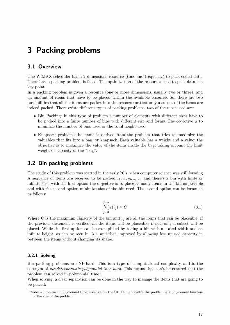
The WiMAX scheduler has a 2 dimensions resource (time and frequency) to pack coded data.Therefore, a packing problem is faced. The optimization of the resources used to pack data is akey point.In a packing problem is given a resource (one or more dimensions, usually two or three), andan amount of items that have to be placed within the available resource. So, there are twopossibilities that all the items are packet into the resource or that only a subset of the items areindeed packed. There exists different types of packing problems, two of the most used are:
• Bin Packing: In this type of problem a number of elements with different sizes have tobe packed into a finite number of bins with different size and forms. The objective is tominimize the number of bins used or the total height used.
• Knapsack problems: Its name is derived from the problem that tries to maximize thevaluables that fits into a bag, or knapsack. Each valuable has a weight and a value; theobjective is to maximize the value of the items inside the bag, taking account the limitweight or capacity of the ”bag“.
3.2 Bin packing problems
The study of this problem was started in the early 70’s, when computer science was still formingA sequence of items are received to be packed i1, i2, i3, ..., in and there’s a bin with finite orinfinite size, with the first option the objective is to place as many items in the bin as possibleand with the second option minimize size of the bin used. The second option can be formuledas follows:
j=n∑j=0
s(ij) ≤ C (3.1)
Where C is the maximum capacity of the bin and ij are all the items that can be placeable. Ifthe previous statement is verified, all the items will be placeable, if not, only a subset will beplaced. While the first option can be exemplified by taking a bin with a stated width and aninfinite height, as can be seen in 3.1, and then improved by allowing less unused capacity inbetween the items without changing its shape.
3.2.1 Solving
Bin packing problems are NP-hard. This is a type of computational complexity and is theacronym of nondeterministic polynomial-time hard. This means that can’t be ensured that theproblem can solved in polynomial time1.When solving, a clear separation can be done in the way to manage the items that are going tobe placed:
1Solve a problem in polynomial time, means that the CPU time to solve the problem is a polynomial functionof the size of the problem
17

3 Packing problems
Figure 3.1: Bin packing
• Online: Items are placed with the order they are in the queue, so there’s no sorting. Theplacement algorithm doesn’t know how will be the items that are coming next, only knowsthe actual one and the ones that have been already placed.
• Offline: In this way, the placement algorithm knows all the elements that should be placedbefore starting the placement itself, sorting is allowed.
To solve bin packing problems various algorithms are defined:
• Next fit (NF): Items are placed in the current level, if fits. If doesn’t a new level is startedand becomes the current one.
• First fit (FF): Items are placed into the lowest indexed initialized level (levels are indexedincreasingly as they are initialized), when an item doesn’t fit in any of the existing levels,a new level is created.
• Best fit (BF): It’s similar to the FF approach, the difference is that here an item is alwaysplaced into the level with lowest residual capacity (when it fits). In case of a tie the itemis placed into the level with the lowest index.
An evolution of these algorithms is the decreasing height option. Items are sorted in a decreasingheight way2, then it’s an offline method.
3.3 Knapsack problems
The main difference between knapsack and bin packing problems is that knapsack problemshave another parameter, it’s the value of each element that’s packed in the bin.There exists two types of knapsack problems bounded or unbounded. Bounded problems restrictthe number of each element to a maximum value and unbounded problems doesn’t have a limiton the number of elements to be placed. There’s a variation from the bounded problem, this isthe 0-1 knapsack problem, where the bound is 1. It can be formuled in this way:
n∑j=1
wjxj ≤ c (3.2)
n∑j=1
pjxj (3.3)
Where xj shows if the object j is selected, and how much of this elements are selected. Theknapsack problem must accomplish the equation 3.2 and also try to maximize the equation
2The first to be placed is the highest, then the second highest, and so on.
18

3.3 Knapsack problems
3.3, where pj is the value of the element.
3.3.1 Solving
To solve knapsack 0-1 problems, there are different types of algorithms to apply.
• Greedy algorithm: Tries to optimize the solution by sorting the values from the greatest tothe lowest, and then placing them in the knapsack. It has low computational complexity,but with this method only can be ensured that half of the values that fits in the optimalsolution will be placed.
• Branch and bonus: This approach is done like an inverse a tree. First is tried to place asmany elements as possible in a greedy way and the backtracking is done, going back inthe tree and looking for the points that can be improved. This is done successively in allthe branches; and at the end all branches are analyzed to look for the one that results ina higher sum of values of the items placed.
• Dynamic programming: This approach divides the optimization problem into smaller prob-lems, and attack them separately.
• Reduction algorithm: Reduce the size of the problem by fixing optimal values to as manyvariables as possible. If placing of not placing an element produces that a solution is worsethat another existing one, then the placement or not of this element will be fixed in allnew possible solutions.
In [13] algorithms are deeply explained and its computational complexity is discussed.
19

3 Packing problems
20

4 Evolutionary algorithms
Since packing problems are NP-hard, an heuristic approach is suitable to solve them, and apossible approach is with evolutionary algorithms (EA).With evolutionary algorithms can’t be ensured that a unique optimal solution will be find, butas more time runs the algorithm a more optimal solution will be the result.
4.1 Overview of evolutionary algorithms
An evolutionary algorithm (EA) uses mechanisms inspired by biological evolution; like repro-duction, mutation, recombination and selection.
Figure 4.1: EA mimics on biological evolution
In figure 4.1, a biological of evolution of giraffes can be seen. Candidate solutions play therole of the individuals in a population (in the example of the figure giraffes).EA rank the kindness of solutions with an objective cost, drawing a parallelism between EAand biological evolution of the figure, the objective function plays the role of the environment,in this case the high trees, this is decide which solutions ”survive” and which don’t.The evolution of the population occur with the application of the mutation and recombination.Recombination is inspired on a sexual reproduction, so the combination of two individuals ofthe population. After evolution fittest solutions remains, like with the giraffes where the longnecked giraffes remain.The power of EA have been demonstrated by solving many problems, some examples are pre-sented:
• Dr Adrian Thompson[19] used EA to produce a voice recognition circuit that can distin-guish between and response to spoken commands using in a FPGA. A random bit stringwas generated and then evolved to get a solution that can distinguish between the spokenwords ”go” and ”stop“. This was done by using only 37 logic gates and without a clock,something that could not be possible by direct human design. Dr Thompson doesn’t knowhow it works, it seems that evolution take advantage of some electromagnetic effects ofthe FPGA cells, moreover if we take into account that 5 logic gates are not connected tothe rest of the circuit.
• Sato et al.[18] used EA to design a concert hall with optimal acoustic properties; maxi-mizing the sound quality for the audience, the conductor and for the musicians. Beginningwith completely rectangular hall, they a leaf-shaped hall as a result. Authors declared
21

4 Evolutionary algorithms
that the solution have similar proportions similar to the Wiener Groβer Musikvereinsaal,considered by experts one of the three finest concert halls in the world.
• He and Mort[20] applied genetic algorithms to find optimal routing paths in telecommu-nication networks. There were multiple parameters to maximize data throughput, mini-mizing transmission delay, finding low-cost paths and distributing load among routers orswitches of the network. In the authors solution the population is initialized with shortestpath solution, which minimizes the number of ”hops”, and congestion or failure was left tothe algorithm. The algorithm was found able to efficiently route around congested links,balancing traffic load and maximizing the total throughput.
There exist various types of evolutionary algorithms, the main differences between them are herepresented:
• Genetic algorithm. This is the most popular type of EA. Seeks for the solution of a problemin the form of a string of numbers and applying recombination operators in addition toselection and mutation.
• Genetic programming. Here solutions are in the form of computer programs, and theirfitness is determined by the ability of the program to solve a computational problem.
• Evolutionary programming. It’s like genetic programming with the difference that thestructure of the program is fixed and the numerical parameters are allowed to evolve.
• Evolution strategy. It works with vectors of real numbers as representations of solutions,typically uses self-adaptive mutation rates.
This thesis will be focused on GA, as is the most commonly used approach and is told as suitableto solve NP-hard problems like packing problems.
4.2 Genetic algorithms
As was told Genetic algorithms (GA) mimics biological evolution. Given a specific problem tosolve, the input of the GA is a set of potential solutions to the problem (population), encodedin some way. These candidates can be randomly generated and delivered or after searching acertain number of solutions. Following, the GA evaluates the solution with a fitness function.The fitness is a quantitative value to the solutions. Best candidates are allowed to continue to thenext generation and reproduce themselves. Reproduction is both asexual; when the individual iscopied but introducing random changes (mutation), or sexual when two individuals are crossedto create new ones (crossover). By repeating this process is expected that the average valueof applying the fitness function to all individuals will increase, and better solutions can bediscovered. In the figure 4.2 are represented which are the steps of a genetic algorithm.
4.2.1 Representation of the solutions
In biological evolution the nature of each individual in a species is coded in its DNA. Each vari-ation in the essence of an individual is coded as a change in the DNA chain. Genetic algorithmsrefers to each solution as a genome, and each one of the elements that codes the solution aregenes. There are various ways to encode solutions in genetic algorithms.
• Numeric representation: This is the most typical approach. Solutions can be coded as abinary string, where the digit at each position represents a value of some aspect of thesolution. Another approach is to code solutions as arrays of integers or decimal numbers,this approach allows greater precision and complexity.
22

4.2 Genetic algorithms
Figure 4.2: Genetic algorithm steps
• List: The coding of the solution is done by a list of objects, the position inside the list ofeach object represents some aspect in the solution. This possibility is particularly suitablefor packing problems, because we can define items to place as objects and define the orderwith are going to be placed as the position in the list.
• Tree structure: Also suitable for packing problems. This is like a list oriented structure,but also using nodes of the tree to define how are the items placed, this structure is definedin [22].
Representation is a key factor in GA. That’s because inside an individual there should only becoded the information of the solution that can improve the solution when changed.A problem in the representation could be the introduction of redundancy into the codificationof the individual. That becomes into an addition of noise when genetic operators are applied,this is because applying a genetic operator will have different effect to characteristics that areredundant in the code to others that are not.
4.2.2 Evolution strategies
Evolution of the population can be done in multiple ways as is done in nature, the most importantones are here presented:
Simple
With this approach, every generation a completely new population. Therefore, all individuals ofthe old generation are replaced by new ones. Drawing a parallelism, this would be like in annualplants or animal species where only the eggs survives the winter.
Steady-state
Generations are progressively renewed. A temporary new generation is created from the old one,the size of the temporary population is defined as a parameter of the genetic algorithm, thispopulation is crossovered and mutated and then joined with the old population. Finally the sizeof the population is fixed to its initial value.
23

4 Evolutionary algorithms
Niche technique
This technique avoids the existence of too many equal individuals in a population to maintainthe genetic diversity of the population. There are various methods defined for this technique (ascan be seen in[21]), the most common are:
• Sharing methods. The fitness value is reduced depending on the. This is done by defininga function that given two individuals returns a value proportional to its likeness1. Thedegree to which to individuals are considered to be of the same species is controlled by thesharing radius; if the distance between to individuals is greater than the sharing radius,they are not occupying the same niche.
• Crowding methods. This method also uses a function that measures the likeness be-tween two genomes individuals, but no radius is defined. An offspring is created from twoindividuals of the population. If the offspring fitness is better that its closest parent, thenew individual replaces the old one.
4.2.3 Genetic operators
To maintain diversity into a population of solutions is necessary to create new solutions fromthe old ones. In genetic algorithms, this is done by mutation and crossover.Further information of the elements presented i this subsection can be found in [14], [15] and[16].
Mutation
Mutation changes one solution individually at a time. A solution is selected randomly applyinga mutation rate, the mutation rate is the probability of one solution to be mutated.Depending on the type of problem, the mutation applied is customized to the individuals ofthe space of solutions. For example in packing of rectangular elements problems, there are thefollowing types of mutators (see [22]).
• Swap mutator: This mutation operator takes two elements of the list and exchange itsposition each other.
• Change mutator: This operator takes one element and maintaining the same area, themutator change its shape. Rectangles can be changed by rotating them, increasing onedimension (and decrease the other one) or randomly change one dimension (and adjustthe other one).
• Swap and change mutator: It’s a combination of the two operators presented before. Twogenes of the genome are selected, swapped and finally mutated.
Both mutation operators can be combined into one operator that does both actions, this is theswap and change mutator.
Crossover
Crossover is a genetic operator inspired in biological sexual reproduction. It takes two individualsof the solution space and combines themselves to create two new solutions that are a mix of thefirst two individuals.For crossover in bin packing, only crossover types that mantains the length of the individualsdoes makes sense, here some types of crossover are presented:
1The likeness is calculated by comparing gene per gene
24

4.2 Genetic algorithms
• N-Point Crossover: With this type of crossover, n points are placed along two encodedsolution (the points are placed in the same position in both solutions), and n+1 sections arecreated. Sections between the points selected are alternately exchanged from one solutionto the other to create two new solutions from the first two ones.
• Partial match crossover: In partial match crossover, two points are selected into the solu-tion. Then, the encoded solution that’s inside the two points are exchanged between thetwo solutions, and the elements that because of the exchange are repeated inside solutionsare changed for the elements that have been lost because of the exchange in its position.
4.2.4 Selection
Fitness function is what provides a measure to realize a selection between the individuals of thepopulation.The first step to obtain the fitness function is by defining an objective function. This functionreturns a score that evaluates how good is a concrete solution from the point of view of thedesigner of the GA.Selection is deeply explained in [17].
Truncation selection
In truncation selection the candidate solutions are ordered by fitness. Then, some proportion p,of the fittest individuals are selected and extended 1/p times to cover the number of individualsof the population.
Roulette wheel selection
In fitness proportionate selection, the fitness function assgins a fitness to possible solutions. Thefitness value is used to associate a probability of selection with each individual chromosome, ascan be seen in equation 4.1, where pi is the probability of being selected, fi is the fitness ofindividual i in the population and N is the total number of individuals in the population.
pi =fi
ΣNj=1fj
(4.1)
Therefore, fitter individuals are more likely to be selected, but there’s still a chance fore someweaker solution to survive the selection process. Another important point for this approach isthat individuals can be selected more than once.It’s called roulette-wheel because it can be conceptually represented as a game of roulette, whereeach individual gets a slice of the wheel, but fitter ones get larger slices than less fit ones.
Rank selection
In this approach each individual in the population is assigned a numerical rank based on fitness,and selection is based on this ranking rather than absolute differences in fitness. The probabilityof being selected depends on the position of the individual in the ranking.The advantage of this method is that it can prevent very fit individuals from gaining dominanceearly at the expense of less fit ones, which would reduce the genetic diversity of the population.
Tournament selection
This type of selection behaves like roulette wheel, but with a defined number (usually 2) indi-viduals of the population. Subgroups of individuals are chosen from the larger population, andthe fittest individual remains ”competes” like in roulette wheel versus the others. Therefore,
25

4 Evolutionary algorithms
with this selection is more likely than fittest solutions remain and population diversity tends toreduce.
4.2.5 Termination Criteria
• The fitness of a solution reaches a minimum stated value.
• A certain number of generations is reached.
• Planned time (budget) is reached.
• The highest ranking solution fitness has reached a value that successive iterations arenot able to increase significantly. The value that measures how is the fitness of solutionsincreasing along iterations is convergence.
26

Part II
Design and simulation
27


5 Description of the problem
As was introduced in section 1.1, the aim of this project is to design a scheduler that tries tooptimize the traffic inside a cell using mobile WiMAX technology.Assuming that a certain amount of users are inside a cell and these users pretend to receivedata by using WiMAX technology. These users have a common resource to share. Concretelya 2 dimensions resource, frequency and time. Therefore the problem is how to pack data fromall users in rectangles within the resource. It’s assumed that there’s only one cell (there’s nointerference) and only one frame is taken into account (retransmissions are not managed).To pack data into a time-frequency rectangle, the first step is to select the transport format forthe codification.As it’s explained in 2.2.3 there are various possible constellations to manage the raw of bits ofdata that a user wants to transmit, choosing the constellation and also the various options ofcode rate (that can be seen in 2.2.2), together transport format. From this election dependsthe number of necessary blocks to pack data1 and the block error rate (BLER) for transmittedblocs would also be affected.This master thesis is focused on the AMC subcarrier and subchannel permutation. Subcarriersare continuously mapped and therefore frequency diversity is lost, as is told in 2.2.4, so thescheduler has to take profit of the frequency bins channel variation of conditions. That meansthat depending on the frequency bins that are being used for a user, this user will have a con-crete effective SINR to transmit its packets. Then, BLER is affected also by the frequency binwhere user’s data is going to be packed. Because of that, selecting the transport format is nottrivial, because changing the transport format also affects the number of necessary bins, andboth parameters affects a key factor of the transmission, BLER. Overlapping the target BLERof the system can produce a dramatically decrease in the overall effective throughput of thesystem2.The problem becomes in a packing problem, without knowing the size, a priory, of the rectanglesthat are going to be packed.As is told in 3.2.1 it’s not possible to solve packing problems linearly, and heuristics have tobe used to solve such type of problems. In this case, the space of solutions will be possibleplacements.Coding how are the rectangles into individuals of a population in a genetic evolution is also akey point. Genetic operators will be customized to affect the parameters of the placement thatcan improve performance. To measure this improvement, the objective function also has to becustomized.And together with the the genetic algorithm elements described; a placement algorithm is nec-essary to get the placement parameters from the coded solution in the genetic algorithm popu-lation3.The problem is done assuming a 10 MHz channel with a consecutive 2 frequency bins and 3symbols association4 and the length of the frame is 5 ms. We assume also a downlink situation,the base station transmits to various mobile stations.
1Logically, as more bits per symbol are coded less resources to transmit the coded will be needed2The target BLER is a parameter that depends on the application and affects the probability of packets dropped3Placement parameters are the values used to calculate the objective functions. Parameters that measures the
goodness of a solution4That’s the mandatory association for AMC defined in the profile, as can be seen in 2.2.4
29

5 Description of the problem
30

6 Problem modelling
This chapter has two differentiated parts. The first one is focused on how the problem is modelled,and the second part concretes more about the details of the software implementation.
6.1 Non-selective approach
Before dealing with the frequency selective approach, a non selective approach was done.The main difference between selective and non-selective approach is that the frequency variationis not managed and then a flat the channel response on all subchannels is assumed. This meansthat a user would use the same codification while transmitting in all frequency bins and also thesame bit error rate. So the description of the problem doesn’t fit within the restrictions of theproblem description, but this approach was used for involving into the packing problems withgenetic algorithms, before dealing with the topic of the master thesis.
6.1.1 Common resource
The common resource for all users is the two dimension space where data is packed. The size ofthe resource has to be stated in some way.The subchannel distribution fixed on AMC profile1 is 2 frequency bins and 3 consecutive symbols(see section 2.2.4), and the number of subcarriers per subchannel is 9, reserving 1 as a pilotsubcarrier and the other ones for data. Assuming a 10 MHz channel and a FFT size of 1024,where 768 are usefull subcarriers. It means that there should be 48 frequency frequency bins.In the time dimension, knowing that the standard number of symbols per WiMAX frame is48, and an AMC subchannel is created with three consecutive symbols, it means that there are16 time divisions in the frame. But it has to be considered that some symbols are reserved fordifferent reasons than placing usefull data. For this approach round numbers near AMC valuesare taken, 50 frequency subchannels and 10 time slots.
6.1.2 Users
With this approach is assumed that there’s not frequency variation, therefore it’s not necessarythat users demand a certain amount of data, they ask directly for the size of the resource thatneed.
6.1.3 Representation of the solutions
The genome is a list of pairs of data. There’s a pointer to the object that is going to be placed(that gives the information about the am mount of subchannnels needed per user) and the widththat will have each rectangle in the solution. The position of each pair of data into list is theorder which objects are placed.
6.1.4 Initialization
The first step for the initialization is to generate the resource demand of each user. This value isassigned by calculating a random (uniformly distributed) integer number between two prefixed
1The non selective approach is done assuming any subcarrier permutation zone. But AMC will be applied in theselective approach, therefore near values of this approach are applied here.
31

6 Problem modelling
bounds. After that, a width value is generated from 1 to either the resource demand of the useror the width of the common resource (the maximum of two values). But some restrictions areapplied, a maximum number of unused subchannels per data pack are allowed, this parameteradjust how much flexibility is given to the creation of rectangles. For example; assume a packof 7 subchannels, if the parameter is fixed to 0, there are only 2 possibilities of packing; settingthe height to 7 or 1 and the width to 1 or 7 respectively. But changing the number of allowedunused subchannels parameter to 1, the use of 7 or 8 subchannels are allowed to pack data andtherefore more possibilities are allowed: the width to 1, 2, 4, 7 or 8 and the inverse values forthe height.
6.1.5 Genetic algorithm
The genetic algorithm selected for this approach is the steady state algorithm. It permits thatgood solutions from old generation remains.Two objective functions are designed to score solutions, depending on the relation between thetotal number of subchannels that users ask for and the subchannels available:
• The total number of subchannels required are more than the available ones. In this casethe objective function takes into account the density of the packing. This is the numberof usefull subchannels (total number of subchannels - unused subchannels) divided for thetotal number of subchannels.
• The total number of subchannels required are less than the available ones. With thissupposition the objective function measures the total height of the placement. For thesame packets placed, the one using less frequency bins, would use resources in a moreoptimal way.
The selection done after scoring solutions is the roulette wheel method, best solutions have morepossibilities to go ahead generations but there are some options for the worse ones, as it’s not adeterministic selection.
6.1.6 Genetic operators
The genetic operators applied are swap and change mutator and partial match crossover.
• Swap and change mutator. With this mutator operator the first step is to select a gene ofthe genome, each gene of the genome can be selected by a rate, the mutation rate Mr. Ifa gene is selected then it’s swapped2 by another randomly selected gene in the genome3.Various change mutator possibilities are designed: rotate rectangles, increase a dimensionor randomly change a dimension.
• Partial match crossover. Two genomes are selected with the probability fixed by thecrossover rate Cr. After that, the two genomes are mixed to create two new offspringswith the system described on subsection 4.2.3.
6.1.7 Placement algorithm
The placement algorithm takes each pair of data in the order that are listed in the genome. Forone side takes the width of the rectangle and for the other side the total number of subchannelsneeded. Once taken the information, the data rectangle is packed from the bottom to the topof the shared resource with a next fit (see subsection 3.2) algorithm variation. Objects are not
2Swapping two elements means that their positions are exchanged3The probability of a gene to be mutated is the mutation rate, but the mutation rate applied gene per gene is
the half of the mutation rate. That’s because the mutation process implies two genes
32

6.2 Frequency selective approach
presorted, it’s an online algorithm. But a kind of decreasing height is also applied. Rectanglesare placed in levels and a new levels are started in these two cases:
• The width of the actual rectangle exceeds the remaining width of the level.
• The height of the actual rectangle exceeds the height of the last rectangle that was placed.
The election of next fit, instead of more optimal procedures, like first fit or best fit, is becausethe aim of the non-selective approach is to be more familiar to packing and genetic algorithmproblems. Applying these other procedures would lead to a more complex implementation.The algorithm is done online because a pre-sorting clips a part of the genetic algorithm. Ifrectangles are always decreasing height ordered, the only element left to the genetic algorithm tooptimize the solution is the width of the rectangles, what reduces the power of genetic algorithms.
6.2 Frequency selective approach
This approach deals with the topic of the master thesis. The design of a frequency selectivescheduler.With this approach the frequency variation is taken into account. Each user ”see” a differentchannel that’s better in some subcarriers than in another ones. Therefore the effective SINR4 isdifferent depending on the subcarrier. Subcarrier permutations like FUSC or PUSC average theSINR of the whole channel by randomly distributing subcarriers through the channel. AMC mapssubcarriers continuously, this fact makes that the transport format selected depends on whichfrequency bins are going to be used to transmit the data packets and therefore the number ofchannels that a user needs are not known a priory. With this approach packets are differentiatedbetween priority and non-priority. Let’s see how this fact affect the modeling.
6.2.1 Common resource
In this approach AMC values are taken into account. The number of frequency bins is 48 (asis explained in subsection 6.1.1). In the time dimension, the number of time slots is 10 (themaximum allowed in a bin is 16). Thereby the shared resource for all users transmitting to acell are 480 subchannels, as can be seen in figure 6.1.
6.2.2 Users
In this case users has to provide more data to the system that in the non-selective approach.
User type
Users can receive priority packets or not priority packets. Priority packets represent data of realtime applications (VoIP, video streaming ...) and non priority packets represent bulk traffic.
Data size
The data size is generated by a randomly distributed function delimited by a lower and an upperbound. These bounds are different depending on the type of data that’s going to be transmitted.Bounds for the real time applications will be lower than ones for bulk applications. That’sbecause real time applications require a continuous transmission with critical time restrictions(restrictions are explained in subsection 2.3.3) and bulk traffic transmit a certain amount ofdata, but without time restrictions.
4The effective SINR is the calculated mean of the SINR in various subcarriers
33

6 Problem modelling
Figure 6.1: Common resource of 480 subchannels
Coding data
Data is coded with FEC blocks, the size of an FEC block depends on the transport used, itcan be consulted in table 6.1. Select the transport format necessary is not a direct procedureinstead of a feedback one.
Transport format Block size (bits) BetaQPSK 1/2 48 1.57QPSK 3/4 72 1.69
16 QAM 1/2 96 4.5616 QAM 3/4 144 7.3364 QAM 2/3 192 2364 QAM 3/4 216 42
Table 6.1: β and FEC block length depending on transport format.
Channel conditions
Each user transmits on a different channel. The channel response for each user is modeled as768 values (one for each subcarrier), calculated in two steps: fast fading simulation for one sideand slow fading and propagation for the other side.The fast fading simulation is done using NLOS empiric outdoor model. To model the slow fadingand propagation a lognormal function is used. Thereafter the two values are multiplied to providethe SINR of a single subcarrier.
6.2.3 Placement algorithm
The placement algorithm is introduced before the representation, because in this case the rep-resentation depends strongly on the election of the placement algorithm. The process is donefor each frequency bin of the resource and for each width possible into the frequency bin (from1 to 10), it’s 480 times per user. It starts by trying the transport format that allows more bitsper symbol, then data is splitted into blocks. And when the hypothetical number of subchan-
34

6.2 Frequency selective approach
nels that are going to be used are known, an hypothetical height of the rectangle is taken andtherefore the frequency bins that are going to be used. Once this is known the SINR for thetransmission is calculated. To calculate the SINR is necessary to average the channel responseof the subcarriers that are going to be used to transmit each FEC block. To calculate this valueexponential effective signal to noise ratio mapping (EESM) is used.
γeff = −β ln(1N
N∑i=1
e−γi/β) (6.1)
EESM is presented in equation 6.1, where β is a constant value that depends on the transportformat (can be consulted in table 6.1), N is the number of subcarriers to average, γi is the SINRof each one of the N subcarriers and γeff .With the SINR, the BLER of each FEC block can be mapped using BLER tables (detailedon appendix B). Therefore the error rate of the whole data packet. If the error rate of thewhole packet is bigger than the maximum error rate allowed, the procedure is repeated withthe following stronger transport code; and so on until there’s a transport format that achievesa lower (or equal) BLER. If there’s not a possible transport format for the user with the widthdefined, then it’s not possible to place the user in the actual frequency bin and the concretewidth. Thereafter the process is repeated with the following width. The maximum error rateallowed is the target BLER and is fixed for each type of data. The target BLER for prioritydata will be lower than for non-priority data. Instead only one frame is simulated, and thereforeno retransmissions are managed, non-priority data is not as critical as priority data. Because ofthat a bigger probability of retransmission is allowed for not real time applications.Overhead is not taken into account, only usefull data.
Position management
At a first sight the placement designed for the non-selective approach could seem also suitablefor the selective approach. But this approach has to deal with the another problem, ensurethe locality of a change in the solution. For a suitable performance of the genetic algorithm isnecessary that a changing a part of the solution (by swapping two elements, for example) onlyaffects the zone of the change. If it affects the whole solution, noise is introduced into the geneticalgorithm and it makes more difficult to improve solutions. By placing from bottom to the topa swap between elements produce that an element can changes its size because of the change ofchannel characteristics, and therefore the transport format (to keep the maximum block errorrate allowed). This effect causes that elements placed above the swapped element, also changesits position and its size. To reduce this effect another placement algorithm is designed.With this new placement algorithm, diagram of the algorithm modelled can be seen in figure6.2, data is not placed from bottom to the top, it’s placed in a frequency bin depending on theposition that’s code in the genome (described in next subsection). Elements are placed on levelsand the procedure of placing data is different if the element that’s going to be placed if it’s thefirst on a level or it’s not. Notice that the level where the element is going to be packed dependson the position code in the gene and if there’s free space in this position, if not placement in thefollowing upper frequency bin is tried.
• First in the level: In this case the packet is tried to be placed by first minimizing the heightof the rectangle. This is, starting with the maximal width of the resource. If it’s possible tobe placed, the width is decreased by one until the height needed for placing the element isincreased; then the following bigger width is selected. In case the element can’t be placedwith maximal width. Placing in the following upper frequency bin is tried.
• Not first in the level: In this case, the process is trying to minimize the width in frontof minimizing the height. Starting with width=1 if the height necessary is lower than the
35

6 Problem modelling
height of the first element, data is packed; if not width is incremented until the heightdoesn’t overlap the height of the first element of the level or the amount of free width inthe level is reached. Then placing in the following upper frequency bin is tried.
Figure 6.2: Diagram of the position management algorithm modelled
The strategy of trying to minimize the height of the firsts of the row is token because providesbetter frequency selectivity to the packing process. Minimizing the number of frequency binsused per user, means reducing the averaging of the channel response and give more freedom tothe genetic algorithm to improve solutions. An alternative to this strategy is try to minimize thetotal number of subchannels used on the packing processes of the firsts of the row, in this way thestrategy is lost but firsts on the row are tried to be placed minimizing number of subchannels.The way how elements are placed in the shared resource also takes into account the order ofthe genes inside the genome. That’s because the position defined for an element to be placedcan be already occupied for another element (that was code firstly in the gene’s list), then theelement is tried to be placed in the upper frequency bins and if the placement algorithm arrivesto the top of the common resource it continues from the bottom; and if it gets another the initialposition, the packet is discarded.
6.2.4 Representation of the solution
As is told in the last subsection, the representation change from the non-selective approach isnecessary to afford the changes in the placement algorithm. Each gene of the genome has areference to the user information (presented on subsection 6.2.2) and the position where thedata will try to pack, concretely where the placement algorithm will start the process.Representation can be seen in figure 6.3, where each colour represents a genome with a referenceto the user (represented for the big number, it’s the user’s identifier), and the little numberrepresents the position assigned.
36

6.2 Frequency selective approach
Figure 6.3: Solution representation
6.2.5 Initialization
The first step is the initialization of the users. Assign the channel conditions to the user (anarray of 768 values, one for each subcarrier), create the number of priority and non-priority usersrequired and depending on the type randomize the number of bits that will be transmitted. Then,a gene is created with a reference to the user and a random position into the 48 frequency binsis assigned.
6.2.6 Genetic algorithm
In this approach both steady state and deterministic crowding strategies are applied. Bothstrategies will be compared in terms of results achieved and time of execution in chapter 7. Theobjective function in this case takes into account the difference between placing priority or notpriority packets, ranking solutions in the following way:
1. Number of priority packets: A placement with more priority packets is better than anotherwith less.
2. Percentage of data placed: With the same number of priority packets placed. The per-centage of the total amount of priority and non-priority data placed is taken into accountwith a weighted sum, giving more importance to the percentage of priority than to thenon-priority. Consider that two placements can pack the same number of priority packets,but placing different packets.
Score = Npr +WprRpr +WnoprRnopr (6.2)
Objective function is presented in equation 6.2, where Npr is the number of priority pack-ets placed, Wpr is the weight given to priority data, Wnopr the weight for non-priority(Wpr+Wnopr=1), Rpr the fraction of priority packets placed and Rnopr the fraction of non-priority packets placed. Roulette wheel selection is applied.
6.2.7 Genetic operators
Swap, change and swap & change are modelled. Swap mutator behaves in the same way thatthe non-selective approach. But, the change operator, changes the frequency bin value for thegene (the frequency bin where the packing algorithm starts the process).In figure 6.4 it can be seen an example of how swap is applied (on the right of the figure)between genes 1 and 4, and thereafter change of the genes is applied. It can be seen for thechange on the colour, but also the position is changed. In gene 4 position is changed from 12 to19 and in gene 1, position is changed from 22 to 34.Swap & change can be done in two ways: change the two elements that have been swappedor swap two elements and then mutate an element. Taking into account that the rate appliedwhen swapping and mutating two elements is the half of the mutation probability required (byswapping one gene, two genes are affected), and when mutating a single element, the mutation
37

6 Problem modelling
rate applied is directly the mutation probability. The first option is the same that was appliedin the non-selective approach and will be called swap & change mutation I and the secondoption will be called swap & change II.
Figure 6.4: Swap & change I. Swap is applied on the left and change on the right of the figure
To apply the change on the position, two possibilities are modelled and will be compared inresults. The new position is extracted randomly from:
• Uniform distributed mutation.
• Normal distributed mutation. The value is extracted from a normal deviation centered inthe old position bin of the gene, the deviation of the normal distribution is a parameterthat must be selected.
Figure 6.5: Partial match crossover
The crossover method used is partial match crossover, this method was explained in subsection4.2.3. In figure 6.5 can be observed how this crossover method is done. Looking at the left partof the figure, two points are selected in both parents, in this case between 3rd and 4th genesare selected, then positions of genomes are related; in the figure gene of user 2 in the father isrelated to gene of user 5 in the mother, that’s because they are the genomes placed in the 4thposition of the other parent. The same happens with the third position, gene of the 1st user ofthe father is related to gene of the 3rd user of the mother. Once relations are done the right partof the figure can be observed, 3rd and 4th gene are exchanged between individuals and to getthe genes that have been lost in the exchange, these are placed in the position where relationwas established, as it was seen in the left part of the figure.
6.2.8 Parameters of the simulation
• Number of users. Total number of users, priority and non priority.
• Number of priority users.
38

6.3 Implementation
• Lower and upper bounds for non-priority data.
• Lower and upper bounds for priority data.
• Target BLER. Different target BLER for priority and non-priority data are allowed.
• Mean and deviation values for the lognormal distribution of the slow fading model.
• Number of generations.
• Size of the population.
• Regeneration value in steady state algorithms.
• Mutation ratio.
• Crossover ratio.
• Deviation of the normal distribution in mutation.
• Weights for the priority and non priority data transmitted in the objective function.
6.3 Implementation
In this section the implementation of the frequency selective model is explained.As was explained previously it’s not possible to calculate an exact solution in a deterministicway. Therefore Monte Carlo methods5 are applied to get reliability of the results.To implement the model C++ language is used and to make the application and get the resultssome libraries that will be introduced in section 6.3.2.
6.3.1 Program structure
As was seen in subsection 6.2.3, the program requires the calculation of the suitable transportformat when a packet is going to placed in the common resource to know which dimensions willhave the packet. This process has to be done for each packet and repeated until the packet canbe placed in a subset of frequency bins. But not only this, the process has to be done for eachgenome of the population, repeated for each generation in the evolution of the genetic algorithmand if we take into account that the algorithm has to be run many times when applying MonteCarlo methods, another step of repetition is added. This induces to think that one concretecalculation of the transport format and the size of the packet in the time/frequency resourcewill be done more than once, therefore CPU time could be wasted. For one user the total numberof placing possibilities are:
Np =i=47∑i=0
48− i = 1152 (6.3)
As there are 48 frequency bins (see subsection 6.2.1) in the common resource, and the packetcan be placed from the bottom to the top, there are 48 possibilities of taking frequency binstogether from the frequency bin 1, 47 from the frequency bin 2, and so on. This number isclearly overlapped by the number of times that the the calculation of the transport formatand the size of the packet from one user will be calculated. Typical numbers for number ofgenerations and size6 of the population are over 100, in the best case 10000 calculations of the
5Monte Carlo methods consists on running an algorithm various times and then compute the solutions togetherto get a mean and a confidence margin of the solutions
6Selection of number of generations and size of the population is a tradeoff between results and time of compu-tation, in chapter 7 is this tradeoff discussed
39

6 Problem modelling
size will be done (assuming that all packets can be directly placed, and the algorithm doesn’thave to go ahead the shared resource) without taking into account the Monte Carlo repetitions.Then, it was seen that’s more optimal to precalculate all the possible placements before theplacing algorithm, to make the placement algorithm faster. But there’s another factor to takeinto account, the memory management.Going deep into the placement process. Only 10 possibilities of placement when starting ona concrete frequency bin have to be saved for the placement process, that’s one placementpossibility for each width possible of the rectangle (see subsection 6.2.1). With a certain widthit’s only interesting to save the possibility that uses less frequency subchannels. Therefore,number of elements that have to be saved per user is reduced to 480, ten values per frequencybin. The intention of the simulation is to evaluate the goodness of the algorithm with variousparameters and not to physically transmit the data packet, because of that the only value thathas to be saved for the placement process would be the hypothetical number frequency binsnecessary when a certain width is fixed and also a starting position, therefore an integer. Whatmeans that 480 bytes for user are necessary to be saved. Assuming a number of users of 50, 24KB of memory would be needed.After these paragraphs, it has been seen that it’s more optimal to precalculate the transportformats and the sizes of the data packets, and after apply this information in the placement.Assuming this, the implementation of the precalculation is separated from the placement.Before the startup phase itself, a model of the fast fading channel is done in Matlab usingthe Winner Project channel models[25]. Winner model is a geometry based stochastic model.Model radio channels based on geometry enables separation of the propagation and anthennaparameters. The channel parameters are based on statistical distributions extracted fromchannel measurement in different scenarios.Winner models permits modelling diverse types of scenarios by changing some parameters. Anarray of 768 columns (one per each subcarrier) and 214 rows is created to be used in the startupphase.
Startup phase
To initialize users, data size is randomized and one of the 214channels created with the Winnermodel is selected by each user.In the startup phase the height that would need a packet to be placed, starting in an hypotheticalfrequency bin and using a concrete width is calculated. To do this for each of the 480 possibilities,the transport formats are iterated, from the one that permits more bits per symbol to thestrongest one. Taking advantage of this process, the best possibility of placing is saved (theplacement that requires less subchannels). With this values a maximum amount of data thatcan be placed in the common resource can be calculated, to compare a placement process withthe best possible placement.Another parameter that’s saved during this phase is the relation between the SINR of thefrequency bins that are used to transmit data over the average SINR of the channel. With thisinformation it can be calculate the improve we get in the channel response with AMC in relationto randomly distributed subcarriers (like PUSC or FUSC), in this case a a 32 bits float is used(assuming 50 users, it’s 96 KB of memory).All the information calculated in the startup phase is saved on files, then will be used in theplacement phase. Diagram of how is the calculation done in the startup phase can be consultedin 6.6.
40

6.3 Implementation
Placement phase
This part of the implementation has two parts; the genetic algorithm and placement algorithm.The placement algorithm is used to score the results in the objective function of the geneticalgorithm.As was told in this section before Monte Carlo methods are used, working in the following way.The genetic algorithm is ran a certain amount of times, calls, and with the average of the resultof the best solution in the last generation we get a batch. By repeating the process o runningthe algorithm the number of calls required, we get various batches. The final result is calculatedby doing the mean of all batches, and also with the different values of the batches, a confidencemargin is calculated.But for the result another value than the score of the objective function presented in subsection6.2.3 is used and it’s calculated in the following way.When initializing the algorithm the best placement for each user calculated in the startup phaseis used. To calculate a maximum bound of data placeable in the common resource, users areranked taking into account:
• User type: Priority packets are ranked in front of non-priority packets.
• Data/subchannels ratio: Inside each type division, packets are ranked depending on howmany data is placed in each subchannel. Therefore, the first packets the ones that cancoded with a transport format that allows more bits per symbol.
With this ranking, packets are selected for this maximum bound placement, until the totalnumber of used subchannels is lower than 480. Notice that it’s not a real placement, becausethe positions of the packets are not taken into account, only the value of subchannels. Then, it’snot ensured that two packets are placed in the same subchannels. It’s a maximum bound, butnot reachable in a real placement. This value is used as a reference.Results are presented as a percentage relation with the data placed in the maximum bound andthe data placed in each result. Notice that this value is only necessary for the best solution ofthe last generation in the genetic algorithm. This is the value managed as result.
R100 = 100Max
Res(6.4)
The 100% mark is then a non-realistic placement and all results will be over this value, the bestvalues will be the nearest values to the 100% mark.Also, when the best solution of the last generation in the genetic algorithm is reached, the meanSINR in the AMC placement over average placement is calculated. It’s done by using the valuessaved for each packet in the startup phase, a geometric mean is calculated with all the packetspacked in a placement.7.In figure 6.7 how a placement looks into the common resource look. This placement has beendone with 20 priority users and 10 non-priority users. The bigger rectangles are non-priorityusers (that transmit bigger amounts of data) packets. Also it’s noticed that there are not all30 packets, that’s because some packets where not able to be packed and are discarded for theframe
6.3.2 Libraries used
To implement the model, two libraries are used. GAlib from the Massachusetts Institute ofTechnology (MIT) and SimLib of the Institute of Communication Networks and Computer En-gineering (IKR) of the University of Stuttgart.
7In appendix A the class diagrams of both program phase implementation can be consulted
41
6 Problem modelling
GAlib
GAlib (genetic algorithms library) is used to implement the genetic algorithm. GAlib providesmost of the possibilities presented on the section 4.2, and also permits an easy customizationof the elements, to achieve the performance of the genetic algorithm for the implementationwanted. In case of the simulation done in this master thesis, the customization has been mainlydone with the representation, the initialization and the genetic operators.More information about GAlib can be found in [23].
IKR Simlib
The simulation control and the management of the statistics has been done with the help of theIKR Simlib. Simlib provides many functionalities to manage simulations, like event handling.With this implementation, it has taken advantage of the simulation control to use Monte Carlomethods, the statistical tool to measure values and the functionalities to parse parameters8 tothe simulation. More information about IKR Simlib can be found in [24].
8Parsing parameters, permits to run a simulation with different parameters automatically, and therefore savingtime
42
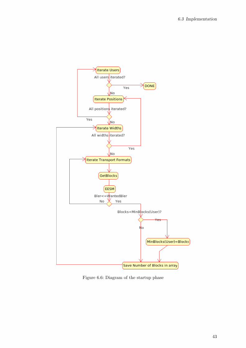
6.3 Implementation
Figure 6.6: Diagram of the startup phase
43

6 Problem modelling
Figure 6.7: Data placement
44

7 Results of the simulation
In this chapter, results of simulation model explained in chapter 6 are presented, and differentvariants are compared.
• Different implementations of genetic operators and evolution strategies introduced in sub-section 6.2.7.
• Parameters of the genetic algorithm.
• Different scenarios, this is different number of priority users and bounds for the random-ization of the size of the data packets for each type of users (priority and non-priority)
Scenario
For all simulations, if anything else is said, following parameters are applied:
• Number of priority and non priority users. Total number of users is 50, and priority useris 30.
• Data size. For priority users bounds for the size randomization selected are 500 and 1500.The upper bound has been selected taking into account a real time application with hightraffic demand, video streaming. Assuming a video quality of 300 kbps, and the fact thata 5 ms frame is used; it results into a need of 1500 bits per frame. For the lower boundVoIP requirements (real time application with low traffic demand) is used. VoIP has adata rate of 14.4 kbps and the maximum allowed delay is 30 ms. That means that VoIPdata can be packed after 6 frames. This result into a need of 216 bits per burst, butassuming that this value is very low and becomes unoptimal (low usefull data ratio) whenadding overhead, 500 bits is selected as the lower bound.Non-priority packets would be bigger than the priority ones, see subsection 6.2.2.Therefore the upper bound of priority type packets (1500) is used as the lower bound fornon-priority type and an upper bound of 6000 is selected.
• Population size and number of generations. The computational complexity is proportionalto the number of generations and population size. The selection of this parameters is atradeoff between the quality of the results and the complexity. Taking into account whatis discussed in a non-selective frame packing problem in OFDMA[26], it has been decidedto fix the parameters of simulation to 100 individuals and 1000 generations. By increasingmore the complexity, the improvement of the results is not significantly.
• Crossover ratio. The effect of crossover ratio seems to have a not very significantly effecton frame packing, see [26]. A crossover ratio of 0.1 is selected then, because it implies lowcomputational time, as less crossovers will be calculated.
• Target BLER. For priority data target BLER is fixed to 0.1 and for non-priority data to0.3.
• Replacement. The value fixed for replacement of generations in the steady-state algorithmis 0.5.
45

7 Results of the simulation
• Mean and deviation for the lognormal that models slow fading and path loss is 13 dB.
• Weights of data types in the objective function. Wp = 0.8 and Wnp = 0.2.
• Calls and batches. The simulations have been done mainly with 25 calls and 20 batches.This is 500 runs to get a mean value and a confidence margin.
7.1 Genetic operators
In this section various types of mutation operators are compared. Firstly, swap, change, swap& change I and swap & change II are compared. Approaches are done, with the first ones, withthe uniform distributed change mutation and then mutation with normal distribution centeredin the old position of the packet.
7.1.1 Swap, change and S&C
Figure 7.1: Swap, change and swap & change results
In figure 7.1; swap, change and swap & change mutators are compared each other, withmutation rates from 0.1 to 0.5 (it’s expected that best results will be achieved with low mutationratios [26]). It can be seen that best results are achieved with swap & change mutator, with aplacement ratio 13 % worst than the maximal placement. Then it’s better to swap and changegenes at the same time, in order to get better results.Another important fact of the results is that the change mutation is far away from the swap andchange, therefore it’s much more important to swap the order of placement than the positionwhere the algorithm starts trying to place the data packet. Another element to be noted is thatas mutation increases swap & changes mutation becomes worse than only swap mutator. That’sbecause swap & change applies a higher amount of mutation with the same rate that swapmutation, and as the mutation parameters increase far from its better value, swap & changesolutions decrease faster.As it couldn’t be seen in figure 7.1 where were the minimums (best performance) for change
and swap and change mutation. In figures 7.2 and 7.3 detail of low mutation ratios are done,respectively. For change mutation it can be observed that minimum is around 0.025 with aplacement ratio near 123%, and for the swap & change minimum values is placed from 0.12 to0.18 mutation rate, being the best value situated in 0.15 with a placement value of 112.4%.Then, for swap and change mutator the best mutation ratio is placed near the 10% mutation.And from change mutator it can be extracted that change without swapping becomes has to bedone in very low rates to get the best results, increasing the probability of changing position of
46
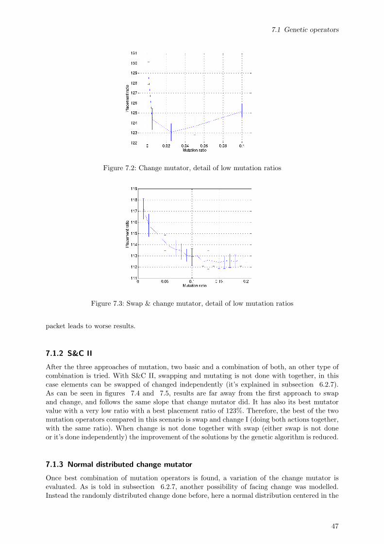
7.1 Genetic operators
Figure 7.2: Change mutator, detail of low mutation ratios
Figure 7.3: Swap & change mutator, detail of low mutation ratios
packet leads to worse results.
7.1.2 S&C II
After the three approaches of mutation, two basic and a combination of both, an other type ofcombination is tried. With S&C II, swapping and mutating is not done with together, in thiscase elements can be swapped of changed independently (it’s explained in subsection 6.2.7).As can be seen in figures 7.4 and 7.5, results are far away from the first approach to swapand change, and follows the same slope that change mutator did. It has also its best mutatorvalue with a very low ratio with a best placement ratio of 123%. Therefore, the best of the twomutation operators compared in this scenario is swap and change I (doing both actions together,with the same ratio). When change is not done together with swap (either swap is not doneor it’s done independently) the improvement of the solutions by the genetic algorithm is reduced.
7.1.3 Normal distributed change mutator
Once best combination of mutation operators is found, a variation of the change mutator isevaluated. As is told in subsection 6.2.7, another possibility of facing change was modelled.Instead the randomly distributed change done before, here a normal distribution centered in the
47

7 Results of the simulation
Figure 7.4: S&C II mutator
Figure 7.5: S&C II mutator, lower mutation ratios detail
old value is applied. In figure 7.6, various deviation parameters are tried for different mutationratios, in a S&C approach (swap and change done at the same time). For values of mutation 20and specially 48, performs in the same way that a uniform distribution; all of the 48 frequencybins are selected with a similar probability. Taking this approach with the lowest mutationratios evaluated (0.1), it can be observed with this mutation that best results are achieved fordeviation=48. In fact, the value is very close to the one obtained by a uniformly distribution.With deviation=1 the value is similar to the (only) swap, mutation as it could be expected (fewchange mutation is done).Trying higher mutations leads to worse results when increasing deviation, that’s because withhigh mutation ratios performance decrease and reducing the deviation of the normal deviationis a way to reduce the mutation effect.It can be concluded that normal distributed change mutator doesn’t improve the performanceof the genetic algorithm.
7.2 Parameter evaluation
In this section the effect of crossover ratio, population size and number of generations areevaluated.
48
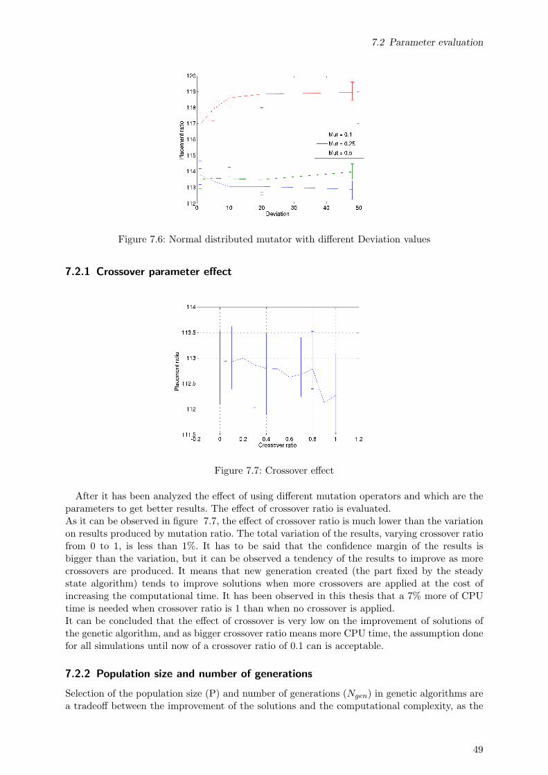
7.2 Parameter evaluation
Figure 7.6: Normal distributed mutator with different Deviation values
7.2.1 Crossover parameter effect
Figure 7.7: Crossover effect
After it has been analyzed the effect of using different mutation operators and which are theparameters to get better results. The effect of crossover ratio is evaluated.As it can be observed in figure 7.7, the effect of crossover ratio is much lower than the variationon results produced by mutation ratio. The total variation of the results, varying crossover ratiofrom 0 to 1, is less than 1%. It has to be said that the confidence margin of the results isbigger than the variation, but it can be observed a tendency of the results to improve as morecrossovers are produced. It means that new generation created (the part fixed by the steadystate algorithm) tends to improve solutions when more crossovers are applied at the cost ofincreasing the computational time. It has been observed in this thesis that a 7% more of CPUtime is needed when crossover ratio is 1 than when no crossover is applied.It can be concluded that the effect of crossover is very low on the improvement of solutions ofthe genetic algorithm, and as bigger crossover ratio means more CPU time, the assumption donefor all simulations until now of a crossover ratio of 0.1 can is acceptable.
7.2.2 Population size and number of generations
Selection of the population size (P) and number of generations (Ngen) in genetic algorithms area tradeoff between the improvement of the solutions and the computational complexity, as the
49

7 Results of the simulation
Figure 7.8: Result evolution with number of generations
Figure 7.9: Result evolution with population size
complexity is directly proportional to these two parameters.Figure 7.8 shows the evolution of the results through the size of the population (notice thatpopulation is logarithmically scaled) with the number of generations fixed at 1000. It can beseen that solutions improves exponentially until a size of 300 hundred, then it slows down andfrom 3000 to 10000 there’s no more improvement. Also the confidence margin of the results is0(all batches have the same mean value). That means that a lower bound has been reached andplacement algorithm can’t go further to 110.9% (10.9% far from the reference value), thereforebigger population sizes doesn’t have sense for this scenario.In this case simulations with a population size of 3000 and 10000 were done with 20 batches5 and 3 calls respectively, to reduce the total time of execution, this fact can explain thatthere’s no confidence margin for this values, but the fact that there’s no evolution from 3000to 10000 and moreover, that another simulation was done with a population of 3000 and also3000 generations and the same result was returned, it seems to mean that a lower bound for theplacement algorithm for this scenario has been really found.Taking into account that the improvement of solutions is reduced over a population size of 300,the balanced point between computational complexity and results achieved seems to be underthis value. Then the assumption for all the simulations done before of a population size of 100seems to be correct.In figure 7.9, the evolution of solutions through the number of generations can be observed,in this case the biggest incremental improve is done from generation 10 to 100, and after thatimprovement slows down. It can also be observed that lowest bound found in figure 7.8 is also
50

7.3 Deterministic crowding
reached in 2000, 5000 and 10000 generations, but each time with a nearer mean to bound anda smaller margin of confidence.With the slow down of the solutions improvement from 1000 and ahead, it would mean thatwhen a reduction of the computational complexity would be required, reduction of the numberof generations could be a good solution two reduce computational without decreasing much thequality of the results.
7.3 Deterministic crowding
Figure 7.10: Deterministic crowding
As it’s told in subsection 4.2.2, deterministic crowding is an evolution strategy that ensuresa bigger genetic variety in populations. Therefore, deterministic crowding is evaluated and com-pared with steady state strategy to notice if there’s an improvement.In figure 7.10 can be observed that the best result achieved is similar than with steady-statestrategy, a mean value of 112.7% is achieved with deterministic crowding in Mr = 0.06 andwith steady state 112.4% was achieved in Mr = 0.15. The results are not improved then, butan expectable fact has occurred. The mutation rate for the best position has been reduced,that’s because deterministic crowding increases diversity and a high mutation rate also does(in another way), then deterministic crowding (as has a bigger genomic variability) needs lessmutation to achieve the required degree of diversity to achieve best results.
7.4 Different scenarios
In this section different scenarios than the one which has been used until now are presented.Scenario II. Working also with 50 users, the number of priority users is reduced to 10 and therest of parameters are leaved with the same values.
For the scenario II the Mr where best results are achieved is in the same zone where it wasfor the scenario I. But, the effect of having more non-priority packets, bigger than the priorityones, is that the placement algorithm loses capacity of placing packets. As the mean size of thepackets increase, less packing possibilities exist.Next, to see how AMC improves SINR in the frequency bins where are placed versus averagingthe whole channel, other scenarios are defined.
• Scenario III. 50 users, 45 of them priority packets. The placement results into a mean size
51

7 Results of the simulation
Figure 7.11: Results over mutation for scenario II
of placed packets of 882 bits1.
• Scenario IV. 10 non-priority users. The placement results into a mean size of 13989 bits2
• Scenario V. 10 non-priority users. The placement results into a mean size of 25320 bits3
Figure 7.12: SINR over averaging the channel with different mean burst sizes
In figure 7.12 can be observed that maximum values of SINR over averaging the whole channelis for smaller packets. That’s because with smaller packets, the scheduler can be more selective,because less bins per packet are used, as the size of packets increase, the scheduler averages agreater number of subchannels. By leading this fact to the maximum (only one packet is placed,using all the subchannels), AMC and FUSC or PUSC subcarrier distribution tends to behavein the same manner.Concretely; 8.4 dBs of improvement are obtained with scenario III, 5.7 dBs with scenario IVand 2.8 dBs with scenario V.
1Bounds for priority: 300 and 1000, non-priority: 1500 and 30002Bounds are: 10000 and 200003Bounds are: 20000 and 30000
52
8 Conclusion and outlook
8.1 Conclusion
As it was presented on chapter 6 a model for the frequency selective scheduler for WiMAXusing genetic algorithms was developed and successfully implemented.Selectiveness leads to packets that are placed without knowing its size in the frequency/timeresource a priory. This fact leaded that a concrete a way of coding solutions to genomes weredeveloped; and following to this solution codification an specific placement algorithm and geneticoperators were modeled.The next challenge faced was the implementation. By dividing the execution of the simulationinto two phases (startup phase and placement phase), computational complexity is reducedwithout a reduction on the performance of the algorithm. Moreover, in real time applications,this approach can be implemented as a parallel work. This is, while the FPGA is calculatingthe packing, it’s calculating the sizes for the placement of next packets. Nevertheless, it has tobe taken into account, that it would be only feasible in case the environment leads a variationof the channel conditions with less quickness to the computing process of calculating sizes.Different variations for mutation operator and evolution strategy were modelled and imple-mented in order to look for a variety of algorithms to face the problem. In chapter 7 thisdifferent models are applied. It has to be said that the approaches customized didn’t improvein a significant manner the results achieved with the algorithm with the standard GAlib imple-mentations. But, at least it was usefull to know that investigation on trying to do a more locallymutation, when implementing a normal distributed change mutation, or ensuring more genomicdiversity, by implementing deterministic crowding, doesn’t deserves the biggest efforts.The effect of genetic operators was also observed. In this way, the crossover doesn’t has a sig-nificantly effect on the evolve of the genetic algorithm, the results variate few when applyingmore or less crossover. Also, a significant fact was seen on genetic operators, this is that betterperformance of the genetic algorithm is achieved when swap and change operators are appliedtogether (depending on the same mutation ratio) and that best results are normally achievedwhen applying a mutation ratio near 10%.Parameters of the genetic algorithms were also proved by running genetic algorithms with vari-ation on these parameters. Two of these parameters are size of the population and number ofgenerations. With these two parameters, the tradeoff between computational complexity andquality of the results is faced. For scenario I it was observed that there was a lower bound thatwhen increasing complexity, genetic algorithm seemed not able to improve. Also, when complex-ity approaches to this value, the incremental improve is significantly reduced. Concretely, it wasseen that running the genetic algorithm over 100 generations (with a fix population of 100) theincremental improvement of solutions highly decrease. A similar effect was observed with thesize of the population, when increasing the size over 300 the improve of the solutions sloweddown.With the design and implementation done it has been proved that near optimal scheduling canbe done with expensive heuristics. With the suitable operators and parameters, a placementonly 10.9% far from the reference value was found. This can be used as reference when doingreal implementations (cheaper heuristics) of the frequency selective scheduler. Knowing how farcan a placement algorithm go without restrictions of complexity can be valuable information. Inthis way it can analyzed, wether it’s usefull to invest resources on improving results or assumethat the bound is close enough.
53

8 Conclusion and outlook
With the same aim of what was exposed last paragraph. A relation of how can AMC improve theSINR of an subcarrier random permutation approach, like FUSC or PUSC, is also presented.This improve, that depends on the mean size of the burst packed in the time/frequency re-source, is also a valuable bound, for nearer to real time applications than the one designed andimplemented in this thesis, to face the tradeoff between quality of the results and computationalcomplexity.
8.2 Outlook
The model designed was able to face the optimization problem of scheduling with frequency se-lectiveness in an environment of 1 frame. Further investigation would be interesting applicationsin a more real case. Doing the simulation for more than one frame leads to be able to manageQoS parameters (delay, jitter, packet dropping probability or bit rate). Simulation of multiplecells would also lead to a more real implementation. By taking into account interference betweenusers of neighbour cells transmitting at the same frequency a further point of view has to betaken to solve the overall problem of trying to find a nearest as possible optimal solutions to allcells. This more realistic approach makes the optimization problem more optimization as moreparameters has to be taken into account, because of that the space of solutions increases andthen heuristics are even more likely to solve the problem.Another path to the objective of a real implementation of the scheduler with genetic algorithmswould be the use of cheaper heuristics, this means reducing the computational complexity. Inthe subsection 7.2.2 it was observed that biggest incremental improve was done from 10 to 100,both in size of the population and number of generations. Therefore, it can be interesting tocenter efforts on working in this zone of computational complexity.The placement algorithm designed was static over generations. It seems reasonable that a dy-namic placement algorithm could face in a better way an optimization problem when usingheuristics, as solutions are better over generations, restrictions of the placement algorithmwould be progressively relaxed. For example, allowing that packets are placed starting froma subchannel situated in the half of an already started level. It would give, without changingthe representation of the solutions, a higher degree of freedom to placement algorithm whenthe space of solutions have already been improved and this can leads to the encounter solutionsthat improves when changing the placement algorithm; and that would be not findable with thestrict behaviour of the placement algorithm.
54

A Selective simulation
In this chapter class diagrams of both parts of the program (startup and placement phase) arepresented.
A.1 Startup phase
Startup phase consists on two classes and a struct. The class diagram can be seen in figure A.1,most important attributes are presented.
Figure A.1: Class diagram of the startup phase
TStartupSimulation
This class manages the simulation. It asks TSelective to calculate values for all users, subchan-nels and widths and saves the option that requires less subchannels per user (that are after usedto calculate reference values for the results).It also deals with opening and closing files. It receive the fading sequence calculated in Matlabwith the winner model and the BLER tables. Then saves the information calculated (heights,mean SINR over averaging the channel, minimal number of subchannels per user and the posi-tions vector that is used to print placements with the help of fill function of Matlab), becauseit can be used on the placement phase.
TSelective
TSelective deals with the calculation of the values. Number of FEC blocks necessaries are cal-culated, EESM methods applied, comparison between burst error rate and target BLER andtherefore transport format and height selection.
TransportFormat
Transport format is a struct used to save the values needed from the different transport formatsused.
55
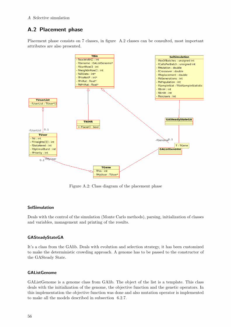
A Selective simulation
A.2 Placement phase
Placement phase consists on 7 classes, in figure A.2 classes can be consulted, most importantattributes are also presented.
Figure A.2: Class diagram of the placement phase
SelSimulation
Deals with the control of the simulation (Monte Carlo methods), parsing, initialization of classesand variables, management and printing of the results.
GASteadyStateGA
It’s a class from the GAlib. Deals with evolution and selection strategy, it has been customizedto make the deterministic crowding approach. A genome has to be passed to the constructor ofthe GASteady State.
GAListGenome
GAListGenome is a genome class from GAlib. The object of the list is a template. This classdeals with the initialization of the genome, the objective function and the genetic operators. Inthis implementation the objective function was done and also mutation operator is implementedto make all the models described in subsection 6.2.7.
56

A.2 Placement phase
TGene
TGene is the template used in GAListGenome class. It has two attributes a pointer to the userwhich the gene is referred to and the position where the placement algorithm would start toplace it.
TUserList
It’s an array of pointers to users. Is used in the initialization process to assign users to genes.
TBin
This class deals with the placement algorithm itself, it receives a reference of the genome tomanage the genes.. With different arrays controls the state of the subchannels. fAccWidth con-trols the accumulated width in each of the frequency bins of the common resource, fStartRowsaves for each frequency bin which is the first frequency bin of its level, fHeightInRow saves theheight of the first element of every level (if there’s no packets placed, then it’s leaved to 0).
TNIHR
It’s the implementation of the the placement algorithm describe NIHR (Not Increasing 1stHeight of the Row) for the class TBin. The placer functions deals with placement algorithmimplementation described.
57

A Selective simulation
58

B BLER tables
BLER tables that maps SINR with BLER values depending on the transport format extractedfrom [27] are here presented.
SINR 0.0 0.5 1.0 1.5 2.0 2.5 3.0 3.5 4.0 4.5 5.0BLER 0.8720 0.629 0.347 0.144 0.0606 0.0363 0.0178 0.0118 0.00838 0.00538 0.00322
Table B.1: BLER table QPSK 1/2
SINR 2.0 2.5 3.0 3.5 4.0 4.5 5.0 5.5 6.0 6.5 7.0BLER 0.999 0.988 0.902 0.652 0.333 0.117 0.0337 0.0133 0.0043 0.00129 0.000645
Table B.2: BLER table QPSK 3/4
SINR BLER5.0 0.9685.5 08276.0 0.5366.5 0.2587.0 0.1297.5 0.07488.0 0.05598.5 0.04139.0 0.0329.5 0.024910.0 0.017810.5 0.0092411.0 0.0064511.5 0.003812.0 0.00193
Table B.3: BLER table 16QAM 1/2
59

B BLER tables
SINR BLER7.0 17.5 18.0 18.5 0.9669.0 0.9419.5 0.69310.0 0.31210.5 0.0911.0 0.022811.5 0.0088112.0 0.0036512.5 0.0027913.0 0.0012913.5 0.00021514.0 0.000215
Table B.4: BLER table 16QAM 3/4
SINR BLER10.0 110.5 111.0 111.5 112.0 0.99812.5 0.96613.0 0.78913.5 0.42514.0 0.15614.5 0.071615.0 0.039815.5 0.024516.0 0.019816.5 0.013517.0 0.010317.5 0.0053718.0 0.00279
Table B.5: BLER table 64 QAM 2/3
60

SINR BLER12.0 112.5 113.0 113.5 0.99914.0 0.98714.5 0.50415.0 0.18615.5 0.054216.0 0.054216.5 0.026917.0 0.019117.5 0.0098918.0 0.0043018.5 0.0017219.0 0.0017219.5 0.0010720.0 0.00107
Table B.6: BLER table 64QAM 3/4
61

B BLER tables
62

C List of figures
63

C List of figures
64

List of Figures
1.1 World internet and cell phone usage statistics, extracted from [1] . . . . . . . . . 11.2 Multipath propagation, extracted from [3] . . . . . . . . . . . . . . . . . . . . . 21.3 Effect of multiple signal arrivals with various delays . . . . . . . . . . . . . . . . 3
2.1 LOS and NLOS . . . . . . . . . . . . . . . . . . . . . . . . . . . . . . . . . . . . . 72.2 Recursive convolutional code scheme with 1/2 rate and constraint length 4 . . . 112.3 QPSK and 16QAM constellation . . . . . . . . . . . . . . . . . . . . . . . . . . . 122.4 OFDMA sub-carrier structure, extracted from [10] . . . . . . . . . . . . . . . . . 122.5 Frame structure, extracted from [10] . . . . . . . . . . . . . . . . . . . . . . . . . 16
3.1 Bin packing . . . . . . . . . . . . . . . . . . . . . . . . . . . . . . . . . . . . . . . 18
4.1 EA mimics on biological evolution . . . . . . . . . . . . . . . . . . . . . . . . . . 214.2 Genetic algorithm steps . . . . . . . . . . . . . . . . . . . . . . . . . . . . . . . . 23
6.1 Common resource of 480 subchannels . . . . . . . . . . . . . . . . . . . . . . . . . 346.2 Diagram of the position management algorithm modelled . . . . . . . . . . . . . 366.3 Solution representation . . . . . . . . . . . . . . . . . . . . . . . . . . . . . . . . . 376.4 Swap & change I. Swap is applied on the left and change on the right of the figure 386.5 Partial match crossover . . . . . . . . . . . . . . . . . . . . . . . . . . . . . . . . 386.6 Diagram of the startup phase . . . . . . . . . . . . . . . . . . . . . . . . . . . . . 436.7 Data placement . . . . . . . . . . . . . . . . . . . . . . . . . . . . . . . . . . . . . 44
7.1 Swap, change and swap & change results . . . . . . . . . . . . . . . . . . . . . . . 467.2 Change mutator, detail of low mutation ratios . . . . . . . . . . . . . . . . . . . . 477.3 Swap & change mutator, detail of low mutation ratios . . . . . . . . . . . . . . . 477.4 S&C II mutator . . . . . . . . . . . . . . . . . . . . . . . . . . . . . . . . . . . . . 487.5 S&C II mutator, lower mutation ratios detail . . . . . . . . . . . . . . . . . . . . 487.6 Normal distributed mutator with different Deviation values . . . . . . . . . . . . 497.7 Crossover effect . . . . . . . . . . . . . . . . . . . . . . . . . . . . . . . . . . . . . 497.8 Result evolution with number of generations . . . . . . . . . . . . . . . . . . . . . 507.9 Result evolution with population size . . . . . . . . . . . . . . . . . . . . . . . . . 507.10 Deterministic crowding . . . . . . . . . . . . . . . . . . . . . . . . . . . . . . . . . 517.11 Results over mutation for scenario II . . . . . . . . . . . . . . . . . . . . . . . . . 527.12 SINR over averaging the channel with different mean burst sizes . . . . . . . . . 52
A.1 Class diagram of the startup phase . . . . . . . . . . . . . . . . . . . . . . . . . . 55A.2 Class diagram of the placement phase . . . . . . . . . . . . . . . . . . . . . . . . 56
65
List of Figures
66

D References
67

D References
68

Bibliography
[1] Internet Telecommunication Union, http://www.itu.int/ITU-D/ict/statistics/
[2] Reuters, global cellphone penetration reaches 50% of the world population,http://investing.reuters.co.uk/news/articleinvesting.aspx?type=media&storyID=nL29172095
[3] Radio communication research group of the Universitat Politecnica de Catalunya,www.gcr.tsc.upc.edu.
[4] Donald C. Cox. 910 MHz Urban Mobile Radio Propagation:Multipath Characteristicsin New York City. IEEE transactions on communications.
[5] Jeffrey G. Andrews, Arunabha Ghosh and Rias Muhamed. Fundamentals of WiMAXUnderstanding Broadband Wireless Networking. Prentice Hall.
[6] Frank Ohrtman. WiMAX handbook Building 802.16 Wireless Networks. McGraw-Hill.
[7] IEEE Std 802.16e-2005 and IEEE Std 802.16-2004/Cor1-2005.
[8] Hassan Yaghoobi. Scalable OFDMA Physical Layer in IEEE 802.16 WirelessMAN.Intel Communications Group.
[9] Govindan Nair, Joey Chou et alt. IEEE 802.16 Medium Access Control and ServiceProvisioning. Intel Communications Group.
[10] WiMAX Forum. Mobile WiMAX Part I: A Technical Overview and PerformanceEvaluation.
[11] WiMAX Forum. Mobile WiMAX Part II: A Comparative Analysis.
[12] WiMAX Forum. Mobile System Profile Release 1.0 Approved Specification (Revision1.4.0: 2007-05-02).
[13] Silvano Martello, Paolo Toth. Knapsack problems, algorithms and computer imple-mentations. John Wiley & Sons.
[14] William B. Langdon and Riccardo Poli. Foundations of genetic programming.Springer.
[15] Karsten Weicker. Evolutionare Algorithmen. Teubner.
[16] Volker Nissen. Einfuhrung in Evolutionare Algorithmen. Vieweg.
[17] David E. Goldberg. Genetic algorithms in search, optimization, and machine learning.Addison-Wesley.
[18] S. Sato et al. Applying genetic algorithms to the optimum design of a concert hall.”Journal of Sound and Vibration, vol.258, no.3, p. 517-526 (2002).
[19] Clive Davidson. ”Creatures from primordial silicon.” New Scientist, vol.156, no.2108,p.30-35 (1997).
69

Bibliography
[20] L. He and N. Mort. ”Hybrid genetic algorithms for telecommunications network back-up routeing.” BT Technology Journal, vol.18, no.4, p. 42-50 (Oct 2000).
[21] Grant Dick. A Comparison of Localised and Global Niching Methods. University ofOtago, Dunedin, New Zealand (2005).
[22] Shian-Miin Hwang. Solving Rectangle Bin Packing Problems Using Genetic Algo-rithm. National Taiwan University,Taipei, Taiwan
[23] Massachussets Institute of Technology. GAlib: A C++ Library of Genetic AlgorithmComponents. http://lance.mit.edu/galib-2.4/
[24] Institute of Communication Networks and Computer Engineering (IKR). IKR Sim-ulation Library-Resources. www.ikr.uni-stuttgart.de/INDSimLib/Resources
[25] Winner Project. http://www.ist-winner.org/.
[26] Marc C. Necker et al. Optimitzed Frame Packing for OFDMA Systems- Institute ofCommunication Networks and Computer Engineering, University of Stuttgart.
[27] WiMAX Forum. WiMAX System Evaluation Methodology (2007).
70

E Appreciations
My deepest thanks go out to University of Stuttgart, IKR and Prof. Dr.-Ing. Dr. h. c. mult.Paul J. Kuhn by giving me the opportunity of writing my master thesis in IKR and let me usethe resources of the Institute.I am indebted to the supervisors of the thesis; Marc Necker, Mathias Kaschub and Elias Doumith,for the help they provided me during the execution of the project.Special appreciation to Universitat Politecnica de Catalunya and Telecom BCN for giving methe opportunity of writing the Master Thesis in University of Stuttgart.My most heartfelt thanks to my parents; Dolors and Joaquim, for their emotional and financialsupport.
71

E Appreciations
72

F Author’s Statement
Hereby I certify that I know and I accept that I have no right to exploit the results of myMaster Thesis by any means without the written permission of the Institute of CommunicationNetworks and Computer Engineering (IKR).
Furthermore, I certify that I have realized this work on my own, and that all sourcesthat I have used or consulted are duly noted herein.
Place and date: Stuttgart, 1st August 2008
Signature:
73