Design of Structural Mechanisms · All of the novel structural mechanisms presented in this...
160
Design of Structural Mechanisms Yan CHEN A dissertation submitted for the degree of Doctor of Philosophy in the Department of Engineering Science at the University of Oxford St Hugh’s College Trinity Term 2003
Transcript of Design of Structural Mechanisms · All of the novel structural mechanisms presented in this...

Design of StructuralMechanisms
Yan CHEN
A dissertation submitted for the degree of Doctor of Philosophy
in the Department of Engineering Science at the University of Oxford
St Hugh’s College
Trinity Term 2003

Design of Structural Mechanisms
AbstractYan CHEN
St Hugh’s College
A dissertation submitted for the degree of Doctor of Philosophy
in the Department of Engineering Science at the University of Oxford
Trinity Term 2003
In this dissertation, we explore the possibilities of systematically constructing large
structural mechanisms using existing spatial overconstrained linkages with only
revolute joints as basic elements.
The first part of the dissertation is devoted to structural mechanisms (networks) based
on the Bennett linkage, a well-known spatial 4R linkage. This special linkage has been
used as the basic element. A particular layout of the structures has been identified
allowing unlimited extension of the network by repeating elements. As a result, a family
of structural mechanisms has been found which form single-layer structural
mechanisms. In general, these structures deploy into profiles of cylindrical surface.
Meanwhile, two special cases of the single-layer structures have been extended to form
multi-layer structures. In addition, according to the mathematical derivation, the
problem of connecting two similar Bennett linkages into a mobile structure, which other
researchers were unable to solve, has also been solved.
A study into the existence of alternative forms of the Bennett linkage has also been
done. The condition for the alternative forms to achieve the compact folding and
maximum expansion has been derived. This work has resulted in the creation of the
most effective deployable element based on the Bennett linkage. A simple method to
build the Bennett linkage in its alternative form has been introduced and verified. The
corresponding networks have been obtained following the similar layout of the original
Bennett linkage.
The second effort has been made to construct large overconstrained structural
mechanisms using hybrid Bricard linkages as basic elements. The hybrid Bricard
linkage is a special case of the Bricard linkage, which is overconstrained and with a
single degree of mobility. Starting with the derivation of the compatibility condition and
the study of its deployment behaviour, it has been found that for some particular twists,
the hybrid Bricard linkage can be folded completely into a bundle and deployed to a flat
triangular profile. Based on this linkage, a network of hybrid Bricard linkages has been
produced. Furthermore, in-depth research into the deployment characteristics, including
kinematic bifurcation and the alternative forms of the hybrid Bricard linkage, has also
been conducted.
The final part of the dissertation is a study into tiling techniques in order to develop a
systematic approach for determining the layout of mobile assemblies. A general
approach to constructing large structural mechanisms has been proposed, which can be
divided into three steps: selection of suitable tilings, construction of overconstrained
units and validation of compatibility. This approach has been successfully applied to the
construction of the structural mechanisms based on Bennett linkages and hybrid Bricard
linkages. Several possible configurations are discussed including those described
previously.
All of the novel structural mechanisms presented in this dissertation contain only
revolute joints, have a single degree of mobility and are geometrically overconstrained.
Research work reported in this dissertation could lead to substantial advancement in
building large spatial deployable structures.
Keywords: Structural mechanism; deployable structure; 3D overconstrained linkage;
network; tiling technique; Bennett linkage; hybrid Bricard linkage;
alternative form.

To My Family

i
Preface
The study contained in this dissertation was carried out by the author in the Department
of Engineering Science at the University of Oxford during the period from January 2000
to August 2003.
First of all, I would like to thank my supervisor, Dr. Zhong You, for his advice,
encouragement and support. He introduced me to the subject of deployable structures.
The regular discussion with him has been very beneficial to my research.
Appreciation also goes to Prof. Sergio Pellegrino and Dr. Simon Guest at the University
of Cambridge, Prof. Eddie Baker at the University of New South Wales of Australia,
Prof. Tibor Tarnai at the Budapest University of Technology and Economics of
Hungary, and Prof. Yunkang Sui at the Beijing Polytechnic University of China. The
advice from them has been invaluable and very helpful to my research.
I am also grateful to the Workshop in the Department of Engineering Science, in
particular, Mr. John Hastings, Mr. Graham Haynes, Mr. Kenneth Howson, and Mr.
Maurice Keeble-Smith. Without their great patience and skill, my models would never
be as impressive as they are.
Financial aid from the K. C. Wong Foundation, ORS and Zonta International, and
conference grants from St Hugh’s College, the Department of Engineering Science and
the University of Oxford are gratefully acknowledged.
Finally, I would like to thank my parents for their confidence in me, and give special
thanks to my husband for all his love, patience and encouragement.

ii
Except for commonly understood and accepted ideas, or where specific reference is
made to the work of others, the contents of this report are entirely my original work and
do not include any work carried out in collaboration. The contents of this dissertation
have not been previously submitted, in part or in whole, to any university or institution
for any degree, diploma, or other qualification.

iii
Contents
1 INTRODUCTION ....................................................................................................... 1
1.1 OVERCONSTRAINED MECHANISMS AND DEPLOYABLE
STRUCTURES ..................................................................................................... 1
1.2 SCOPE AND AIM................................................................................................ 3
1.3 OUTLINE OF DISSERTATION ......................................................................... 4
2 REVIEW OF PREVIOUS WORK ............................................................................ 6
2.1 LINKAGES AND OVERCONSTRAINED LINKAGES.................................... 6
2.2 3D OVERCONSTRAINED LINKAGES............................................................. 8
2.2.1 4R Linkage - Bennett Linkage....................................................................... 9
2.2.2 5R Linkages ................................................................................................ 15
2.2.3 6R Linkages ................................................................................................ 17
2.2.4 Summary ..................................................................................................... 33
2.3 TILINGS AND PATTERNS .............................................................................. 35
2.3.1 General Tilings and Patterns...................................................................... 35
2.3.2 Tilings by Regular Polygons....................................................................... 37
2.3.3 Summary – 3 Types of Simplified Tilings ................................................... 42
3 BENNETT LINKAGE AND ITS NETWORKS..................................................... 45
3.1 INTRODUCTION .............................................................................................. 45
3.2 NETWORK OF BENNETT LINKAGES .......................................................... 46
3.2.1 Single-layer Network of Bennett Linkages ................................................. 46
3.2.2 Multi-layer Network of Bennett linkages .................................................... 57
3.2.3 Connectivity of Bennett Linkages ............................................................... 62
3.3 ALTERNATIVE FORM OF BENNETT LINKAGE ........................................ 67
3.3.1 Alternative Form of Bennett Linkage ......................................................... 67
3.3.2 Manufacture of Alternative Form of Bennett linkage................................. 80

iv
3.3.3 Network of Alternative Form of Bennett Linkage....................................... 93
3.4 CONCLUSION AND DISCUSSION................................................................. 94
4 HYBRID BRICARD LINKAGE AND ITS NETWORKS ................................... 96
4.1 INTRODUCTION .............................................................................................. 96
4.2 HYBRID BRICARD LINKAGES...................................................................... 97
4.3 NETWORK OF HYBRID BRICARD LINKAGES ........................................ 103
4.4 BIFURCATION OF HYBRID BRICARD LINKAGE.................................... 109
4.5 ALTERNATIVE FORMS OF HYBRID BRICARD LINKAGE .................... 116
4.6 CONCLUSION AND DISCUSSION............................................................... 123
5 TILINGS FOR CONSTRUCTION OF STRUCTURAL MECHANISMS........ 125
5.1 INTRODUCTION ............................................................................................ 125
5.2 NETWORKS OF BENNETT LINKAGES ...................................................... 126
5.2.1 Case A....................................................................................................... 126
5.2.2 Case B....................................................................................................... 127
5.2.3 Case C....................................................................................................... 130
5.3 NETWORKS OF HYBRID BRICARD LINKAGES ...................................... 131
5.3.1 Case A....................................................................................................... 131
5.3.2 Case B....................................................................................................... 132
5.3.3 Case C....................................................................................................... 133
5.4 CONCLUSION AND DISCUSSION............................................................... 135
6 FINAL REMARKS.................................................................................................. 136
6.1 MAIN ACHIEVEMENTS................................................................................ 136
6.2 FUTURE WORKS............................................................................................ 138
REFERENCE.............................................................................................................. 141

v
List of Figures
2.1.1 Coordinate systems for two links connected by a revolute joint. ........................... 8
2.2.1 Original model of the Bennett linkage.................................................................. 10
2.2.2 A schematic diagram of the Bennett linkage. ....................................................... 10
2.2.3 Goldberg 5R Linkages. (a) Summation; (b) subtraction....................................... 16
2.2.4 Myard Linkage...................................................................................................... 16
2.2.5 Double-Hooke’s-joint linkage. (a) A schematic diagram; (b) sketch of a practical
model................................................................................................................... 18
2.2.6 Sarrus linkage. (a) Model by Bennett; (b) a schematic diagram. ......................... 19
2.2.7 Bennett 6R hybrid linkage. ................................................................................... 20
2.2.8 Bennett plano-spherical hybrid linkage. ............................................................... 20
2.2.9 Bricard linkages. (a) Trihedral case; (b) line-symmetric octahedral case.. .......... 22
2.2.10 A kaleidocycle made of six tetrahedra................................................................ 24
2.2.11 Goldberg 6R linkages. (a) Combination; (b) subtraction; (c) L-shaped; (d)
crossing-shaped................................................................................................... 25
2.2.12 Altmann linkage.................................................................................................. 26
2.2.13 Waldron hybrid linkage from two Bennett linkages........................................... 28
2.2.14 Schatz linkage. .................................................................................................... 29
2.2.15 Turbula machine.. ............................................................................................... 29
2.2.16 Wohlhart 6R linkage. .......................................................................................... 30
2.2.17 Wohlhart double-Goldberg linkage. ................................................................... 31
2.2.18 Bennett-joint 6R linkage. .................................................................................... 32
2.3.1 A honeycomb of bees. .......................................................................................... 36
2.3.2 Escher’s Woodcut ‘Sky and Water’ in 1938. ....................................................... 36
2.3.3 The edge-to-edge monohedral tilings by regular polygons... ............................... 38
2.3.4 Eight distinct edge-to-edge tilings by different regular polygons. ....................... 39
2.3.5 Examples of 2-uniform tilings .............................................................................. 41
2.3.6 An example of equitransitive tilings..................................................................... 41

vi
2.3.7 Tilings that are not edge-to-edge. ......................................................................... 43
2.3.8 Pattern with overlapping motifs............................................................................ 43
2.3.9 Units, represented by grey dash lines, in tilings and patterns............................... 44
3.2.1 A schematic diagram of the Bennett linkage. ....................................................... 46
3.2.2 Single-layer network of Bennett linkages. (a) A portion of the network; (b)
enlarged connection details................................................................................. 47
3.2.3 Network of Bennett linkages with the same twists............................................... 52
3.2.4 Network of similar Bennett linkages with guidelines........................................... 52
3.2.5 A special case of single-layer network of Bennett linkages. (a) – (c) Deployment
sequence; (d) view of cross section of network.. ................................................ 53
3.2.6 aR / vs θ for different t ( abt /= ). ................................................................... 54
3.2.7 (a) – (c) Deployment sequence of a deployable arch............................................ 55
3.2.8 (a) – (c) Deployment sequence of a flat deployable structure. ............................. 56
3.2.9 A basic unit of Bennett linkages. (a) A basic unit of single-layer network; (b) part
of multi-layer unit; (c) the other part; (d) a basic unit of multi-layer network. .. 57
3.2.10 (a) – (c) Deployment sequence of a multi-layer Bennett network...................... 61
3.2.11 Connection of two similar Bennett linkages by four revolute joints at locations
marked by arrows................................................................................................ 62
3.2.12 Connection of two Bennett linkages ABCD and WXYZ. (a) Addition of four
bars; (b) a complementary set; (c) further extension; (d) formation of the inner
Bennett linkage. .................................................................................................. 63
3.2.13 Two similar Bennett linkages connected by four smaller ones. ......................... 65
3.2.14 (a) – (c) Three configurations of connection of two similar Bennett linkages. .. 66
3.3.1 A Bennett linkage. ................................................................................................ 68
3.3.2 Equilateral Bennett linkage. Certain new lines are introduced in (a), (b) and (c)
for derivation of compact folding and maximum expanding conditions. ........... 69
3.3.3 dθ vs fθ for a set of given α . ............................................................................. 76
3.3.4 lL / , lc / and ld / vs fθ when 12/7πα = . ....................................................... 76
3.3.5 δ vs fθ when 12/7πα = . .................................................................................. 77
3.3.6 α vs fθ when the fully deployed structure based on the alternative form of the
Bennett linkage forms a square........................................................................... 79

vii
3.3.7 The alternative form of Bennett linkage made from square cross-section bars in
the deployed and folded configurations.. ............................................................ 80
3.3.8 The alternative form of Bennett linkage with square cross-section bars in
deployed configuration. ...................................................................................... 81
3.3.9 The geometry of the square cross-section bar. (a) In 3D; (b) projection on the
plane x'o'y' and the cross section RXYZ............................................................. 83
3.3.10 λ vs ω for a set of given α . ............................................................................. 85
3.3.11 The alternative form of Bennett linkage with square cross-section bars in folded
configuration. ...................................................................................................... 86
3.3.12 Model that 6/πλ = and 180/53πω = . ............................................................ 89
3.3.13 Model that 6/πλ = and 4/πω = . ................................................................... 90
3.3.14 Model that 4/πλ = and 4/πω = ..................................................................... 91
3.3.15 Model that 4/πλ = and 3/πω = ..................................................................... 92
3.3.16 Network of alternative form of Bennett linkage................................................. 94
4.2.1 Hybrid Bricard linkage. ........................................................................................ 97
4.2.2 ϕ vs θ for the hybrid Bricard linkage for a set of α in a period. ....................... 98
4.2.3 Deployment sequence of a hybrid Bricard linkage with 4/πα = . (a) The
configuration of planar equilateral triangle; (b) the configuration in which the
movement of linkage is physically blocked...................................................... 100
4.2.4 Deployment sequence of a hybrid Bricard linkage with 12/5πα = . (a) The
configuration of planar equilateral triangle; (b) and (c) the configurations during
the process of movement. ................................................................................. 101
4.2.5 Deployment sequence of a hybrid Bricard linkage with 3/πα = . (a) The compact
folded configuration; (b) the configuration during the process of deployment; (c)
the maximum expanded configuration.............................................................. 102
4.3.1 (a) Schematic diagram of the hybrid Bricard linkage; (b) one pair of the cross bars
connected by a hinge in the middle................................................................... 103
4.3.2 Construction of the deployable element. (a) Two possible pairs of cross bars: type
A and B; (b) one of the arrangements: A-A-B.................................................. 104
4.3.3 Connectivity of deployable elements.................................................................. 105
4.3.4 Model of connectivity of deployable elements with a type A pair. (a) Fully
deployed; (b) during deployment; and (c) close to being folded. ..................... 106

viii
4.3.5 Model of connectivity of deployable elements with a type B pair. (a) Fully
deployed; (b) during deployment...................................................................... 107
4.3.6 Portion of a network of hybrid Bricard linkages. ............................................... 107
4.3.7 Model of a network of hybrid Bricard linkages.................................................. 108
4.4.1 The compatibility paths of the hybrid Bricard linkage. (a) 3/2πα = and
επα ±= 3/2 ; (b) παπ ≤≤2/ ....................................................................... 110
4.4.2 A typical hybrid Bricard linkage. ....................................................................... 111
4.4.3 Equilibrium of links and joints. (a) Forces and moments in two typical links; (b)
forces and moments at joints 2 and 3................................................................ 112
4.5.1 The alternative form of hybrid Bricard linkage. ................................................. 116
4.5.2 A hybrid Bricard linkage in its alternative from. (Courtesy of Professor Pellegrino
of Cambridge University). ................................................................................ 118
4.5.3 Deployment of Linkage I. (a) Fully expanded configuration; (b) blockage occurs
during folding.................................................................................................... 120
4.5.4 Deployment of Linkage II. (a) Fully expanded; (b) – (c) intermediate; (d) fully
folded configurations. ....................................................................................... 120
4.5.5 The compatibility path of the 6R linkage with twist 2arctan−= πα . .............. 121
4.5.6 Card model of Linkage I. (a) At D, (b) B, (c) E and (d) F′ of the compatibility
path.................................................................................................................... 122
5.2.1 (a) A Bennett linkage; (b) two Bennett linkages connected. .............................. 127
5.2.2 (a) A unit based on the Bennett linkage; (b) network of units............................ 128
5.2.3 A unit based on the Bennett linkage. .................................................................. 131
5.3.1 A network of hybrid Bricard linkage.................................................................. 132
5.3.2 (a) A hybrid Bricard linkage with twists of 3/π or 3/2π ; (b) possible
connections; (c) and (d) projection of probable deployment sequence. ........... 133
5.3.3 A unit based on the hybrid Bricard linkage. ....................................................... 134
5.3.4 Projection of a network of hybrid Bricard linkages during deployment. ........... 134

ix
Notation
C: cosine.
S: sine.
[ ]I : Unit matrix.
K : Number of distinct k-uniform tilings.
L : Actual side length of the alternative form of the linkage.
Li : Loop i of Bennett linkage or hybrid Bricard linkage in the possible
network.
ijMx : Moment at joint i of link ij in local coordination xij.
ijMy : Moment at joint i of link ij in local coordination yij.
ijMz : Moment at joint i of link ij in local coordination zij.
ijNx : Force at joint i of link ij in local coordination xij.
ijNy : Force at joint i of link ij in local coordination yij.
ijNz : Force at joint i of link ij in local coordination zij.
R : Radius of the deployed cylinder of the network of Bennett linkages.
iR : Distance from link ji to link ik positively about iZ . Also referred as
offset of joint i .
][ jiT : Transfer matrix between system of link jj )1( − and system of link
ii )1( − .
iX : Axis commonly normal to jZ and iZ , positively from joint j to joint i .
iZ : Axis of revolute joints i , i could be number or letter.
a : Length of links of a Bennett linkage, or length of links of other linkages.
ia : Length of links of Bennett linkage i .
jia : Distance between axes jZ and iZ . Also referred as length of link ji .

x
b : Length of links of a Bennett linkage, or length of links of other linkage.
ib : Length of links of Bennett linkage i .
c : Distance between joint of the original linkage and that of the alternative
form of the original linkage along the axis of joint.
d : Distance between joint of the original linkage and that of the alternative
form of the original linkage along the axis of joint.
f : Number of the kinematic variables of a joint.
k : Number of transitivity classes with respect to the group of symmetries of
the tilings.
Bk : Bennett ratio of a Bennett joint.
Sk : Ratio of lengths of two similar Bennett linkages.
ik : Ratio of lengths of two Bennett linkages, i = 1, 2, 3, 4.
l : Length of links of an equilateral Bennett linkage, or length of links of a
hybrid Bricard linkage.
link ji : Link connecting joint j and joint i .
m : Mobility of a linkage.
n : Number of links of the linkage.
p : Number of joints of the linkage.
t : Ratio of two lengths of a Bennett linkage, ab / .
α : Twist of links of Bennett linkage or the twist of links of hybrid Bricard
linkage.
iα : Twist of a link of Bennett linkage i .
jiα : Angle of rotation angle from axes jZ to iZ positively about axis iX .
Also referred as twist of link ji .
β : Twist of links of Bennett linkage or the twist of links of hybrid Bricard
linkage.
iβ : Twist of a link of Bennett linkage i .
δ : Angle between two adjacent sides of the alternative form of Bennett
linkage.
ε : A small imperfection.

xi
φ : Revolute variables of a linkage.
dγ : Geometric parameter.
fγ : Geometric parameter.
ϕ : Revolute variable of a linkage.
dϕ : Revolute variable of a linkage when the alternative form of the linkage is
in its fully deployed configuration.
fϕ : Revolute variable of a linkage when the alternative form of the linkage is
in its fully folded configuration.
λ : Angle of rotation of a square cross-section bar along its central axis.
µ : Geometric parameter.
ν : Geometric parameter.
θ : Revolute variable of a linkage.
dθ : Revolute variable of a linkage when the alternative form of the linkage is
in its fully deployed configuration.
fθ : Revolute variable of a linkage when the alternative form of the linkage is
in its fully folded configuration.
iθ : Revolute variable of the linkage, which is the angle of rotation from 1−iX
to iX positively about iZ .
σ : Revolute variable of the linkage.
τ : Revolute variable of the linkage.
υ : Revolute variable of the linkage.
ω : Half of the angle between two adjacent sides of the alternative form of
the Bennett linkage, which is 2/δ .
dξ : Geometric parameter.
fξ : Geometric parameter.
I : Type of similar Bennett linkages in mobile network of Bennett linkages.
Ij : Type of similar Bennett linkages in mobile network of Bennett linkages.
IIi : Type of similar Bennett linkages in mobile network of Bennett linkages.
− IIi : Type of similar Bennett linkages in mobile network of Bennett linkages
whose twists have opposite sign to those of IIi.

1
1
Introduction
1.1 OVERCONSTRAINED MECHANISMS AND DEPLOYABLE
STRUCTURES
A mechanism is commonly identified as a set of moving or working parts in a machine
or other device essentially as a means of transmitting, controlling, or constraining
relative movement. A mechanism is often assembled from gears, cams and linkages,
though it may contain other specialised components, such as springs, ratchets, brakes,
and clutches, as well. Reuleaux published the first book on theoretical kinematics of
mechanisms in 1875 (Hunt, 1978). Later on the general mobility criterion of an
assembly was established by Grübler in 1921 and Kutzbach in 1929, respectively
(Phillips, 1984), based on the topology of the assembly.
However, it was found that this criterion is not a necessary condition. Some specific
geometric condition in an assembly could make it a mechanism even though it does not
obey the mobility criterion. This type of mechanisms is called an overconstrained
mechanism. The first published research on overconstrained mechanisms can be traced
back to 150 years ago when Sarrus discovered a six-bar mechanism capable of
rectilinear motion. Gradually more overconstrained mechanisms were discovered by

Chapter 1 Introduction
———————————————————————————————————
2
other researchers in the next half a century. However, most overconstrained
mechanisms have rarely been used in industrial applications because of the development
of gears, cams and other means of transmission, except two of them: the double-
Hooke’s-joint linkage, which is widely applied as a transmission coupling, and the
Schatz linkage, which is used as a Turbula machine for mixing fluids and powders.
Over the recent half century, very few overconstrained mechanisms have been found.
Most research work on overconstrained mechanisms is mainly focused on their
kinematic characteristics.
During the same period, a new branch of structural engineering, deployable structures,
started its rapid development. Deployable structures are a novel and unique type of
engineering structure, whose geometry can be altered to meet practical requirements.
Large aerospace structures, e.g. antennas and masts, are prime examples of deployable
structures. Due to their size, they often need to be packaged for transportation and
expanded at the time of operation. The deployment of such structures can rely on the
large deformation or the concept of mechanisms, i.e. the structures are assemblies of
mechanisms whose mobility is retained for the purpose of deployment. The latter are
also called structural mechanisms. The key advantage of structural mechanisms is that
they allow repeated deployment without inducing any strain in their structural
components. In the selection of mechanisms, overconstrained geometry is preferred
because it provides extra stiffness, as most such structures are for aerospace applications
in which structural rigidity is one of the prime requirements. Furthermore, these
structural mechanisms often have only hinged connections due to the fact that this kind
of linkage provides more robust performance than sliders or other types of connections.

Chapter 1 Introduction
———————————————————————————————————
3
Research into the construction of structural mechanisms has a completely different
focus from the study of mechanisms. Kinematic characteristics such as the trajectory
described by a mechanism become less important. Instead, the keys to a successful
concept are, first of all, to identify a robust and scalable building block made of simple
mechanisms; and secondly, to develop a way by which the building blocks can be
connected to form a large deployable structure while retaining the single degree of
freedom. In this process, one has to ensure that the entire assembly satisfies the
geometric compatibility.
Research in this area over the last three decades has primarily focused on the
construction of structural mechanisms using planar mechanisms, e.g. the foldable bar
structures (You and Pellegrino, 1993 and 1997) and the Pactruss structures (Rogers, et
al., 1993). The building blocks involve one or more types of basic planar mechanisms of
single mobility. The structures are then assembled in a way that geometric compatibility
conditions are met. 3D mechanisms are rarely used, probably due to the mathematical
difficulty of dealing with non-linear geometric compatibility conditions in 3D.
1.2 SCOPE AND AIM
The aim of this dissertation is to explore the possibility of constructing structural
mechanisms using existing 3D overconstrained linkages, i.e. mechanisms connected by
revolute joints, and the mathematical tiling technique.
Chapter 1 Introduction
———————————————————————————————————
4
In this process, we first examine the existing 3D overconstrained linkages and divide
them into two groups: basic linkages and derivatives of the basic linkages. Then we
concentrate on basic linkages and identify possible ways to assemble them using the
mathematical tiling technique. Finally, we look into the structural mechanisms obtained,
examine their profiles and explore their potential applications.
1.3 OUTLINE OF DISSERTATION
This dissertation consists of six chapters.
Chapter 2 presents a brief review of existing work related to our task, including the
definitions and analysis methods for overconstrained linkages, the existing 3D
overconstrained linkages, as well as the mathematical tiling technique. The reason for
including tiling in this review is because it is used later in producing a suitable
arrangement of basic linkages in order to build structural mechanisms.
Chapter 3 focuses on the construction of structural mechanisms using the Bennett
linkage. First of all, a method to form a network of Bennett linkages is presented. This
is followed by the mathematical derivation of the compact folding and maximum
expanding conditions, which leads to the discovery of an alternative form of the Bennett
linkage. The alternative is then extended to networks of Bennett linkages, leading to
large structural mechanisms which can be compactly folded up. This chapter is ended
with further discussion and conclusions.

Chapter 1 Introduction
———————————————————————————————————
5
Chapter 4 is devoted to the design of structural mechanisms using the hybrid Bricard
linkage. Firstly, the construction process of a 6R hybrid linkage based on the Bricard
linkage and its basic characteristics are described. Secondly, the deployment features
and the possibilities to form networks of hybrid Bricard linkage are presented. Thirdly,
the bifurcation of this linkage is studied. Furthermore alternative forms of the hybrid
Bricard linkage are discussed. Finally an in-depth discussion ends this chapter.
Chapter 5 deals with the mathematical tiling technique and its application in the
construction of structural mechanisms. The networks of Bennett linkages and hybrid
Bricard linkages are revisited according to the tiling technique.
The main achievements of the research are summarised in Chapter 6, together with
suggestions for future work, which conclude this dissertation.

6
2
Review of Previous Work
2.1 LINKAGES AND OVERCONSTRAINED LINKAGES
A linkage is a particular type of mechanism consisting of a number of interconnected
components, individually called links. The physical connection between two links is
called a joint. All joints of linkages are lower pairs, i.e. surface-contact pairs, which
include spherical joints, planar joints, cylindrical joints, revolute joints, prismatic joints,
and screw joints. Here we limit our attention to linkages whose links form a single loop
and are connected only by revolute joints, also called rotary hinges. These joints allow
one-degree-of-freedom movement between the two links that they connect. The
kinematic variable for a revolute joint is the angle measured around the two links that it
connects.
From classical mobility analysis of mechanisms, it is known that the mobility m of a
linkage composed of n links that are connected with p joints can be determined by the
Kutzbach (or Grübler) mobility criterion (Hunt, 1978):
( ) ∑+−−= fpnm 16 (2.1.1)
where ∑ f is the sum of kinematic variables in the mechanism.

Chapter 2 Review of Previous Work
———————————————————————————————————
7
For an n-link closed loop linkage with revolute joints, np = , and the kinematic variable
nf =∑ . Then the mobility criterion in (2.1.1) becomes
6−= nm (2.1.2)
So in general, to obtain a mobility of one, a linkage with revolute joints needs at least
seven links.
It is important to note that (2.1.2) is not a necessary condition because it considers only
the topology of the assembly. There are linkages with full-range mobility even though
they do not meet the mobility criterion. These linkages are called overconstrained
linkages. Their mobility is due to the existence of special geometry conditions among
the links and joint axes that are called overconstrained conditions.
Denavit and Hartenberg (Beggs, 1966) set forth a standard approach to the analysis of
linkages, where the geometric conditions are taken into account. They pointed out that,
for a closed loop in a linkage, the necessary and sufficient mobility condition is that the
product of the transform matrices equals the unit matrix, i.e.,
[ ] [ ][ ][ ] [ ]ITTTTn =1223341 K (2.1.3)
where ][ )1( +iiT is the transfer matrix between the system of link ii )1( − and the system of
link )1( +ii , see Fig. 2.1.1,
[ ]
−−−−
−=
++++
++++
++
)1()1()1()1(
)1()1()1()1(
)1()1(
00001
iiiiiiiiiii
iiiiiiiiiii
iiiiii
CCSSSCRSCCSCSR
SCaT
αθαθαααθαθαα
θθ(2.1.4)
When ni >+1 , 1+i is replaced by 1.

Chapter 2 Review of Previous Work
———————————————————————————————————
8
i
Ri
i-1ai( +1)i
//Zi-1Zi-1
Zi
//ZiZi+1
Xi+1Yi+1
i+1
//Xi
XiYi
i
i i( +1)
( -1)i i a( -1)i i
Fig. 2.1.1 Coordinate systems for two links connected by a revolute joint.
Note that the transfer matrix between the system of link )1( +ii and the system of link
ii )1( − is the inverse of ][ )1( +iiT . That is
[ ] [ ]
−−
−==
++
+++
+++−
++
)1()1(
)1()1()1(
)1()1()1(1
)1()1(
0
0001
iiiii
iiiiiiiiii
iiiiiiiiiiiiii
CSRCSCCSSa
SSSCCCaTT
ααθαθαθθ
θαθαθθ(2.1.5)
2.2 3D OVERCONSTRAINED LINKAGES
The minimum number of links to construct a mobile loop with revolute joints is four as
a loop with three links and three revolute joints is either a rigid structure or an
infinitesimal mechanism when all three revolute axes are coplanar and intersect at a
single point (Phillips, 1990). So 3D overconstrained linkages can have four, five or six

Chapter 2 Review of Previous Work
———————————————————————————————————
9
links. When these linkages consist of only revolute joints, they are called 4R, 5R or 6R
linkages.
The first overconstrained mechanism which appeared in the literature was proposed by
Sarrus (1853). Since then, other overconstrained mechanisms have been proposed by
various researchers. Of special interest are those proposed by Bennett (1903), Delassus
(1922), Bricard (1927), Myard (1931), Goldberg (1943), Waldron (1967, 1968 and
1969), Wohlhart (1987, 1991 and 1993) and Dietmaier (1995). Phillips (1984, 1990)
summarised all of the known overconstrained mechanisms in his two-volume book.
However, the most detailed studies of the subject of overconstraint in mechanisms are
due to Baker (1980, 1984, etc.).
2.2.1 4R Linkage - Bennett Linkage
Common 4R mobile loops can normally be classified into two types: the axes of rotation
are all parallel to one another, or they are concurrent, i.e. they intersect at a point,
leading to 2D 4R or spherical 4R linkages, respectively. Any disposition of the axes
different from these two special arrangements is known usually to be a chain of four
pieces which is, in general, completely rigid and so furnishes no mechanism at all. But
there is an exception, which is the Bennett linkage (Bennett, 1903).
The Bennett linkage is a skewed linkage of four pieces having the axes of revolute
joints neither parallel nor concurrent. Figure 2.2.1 shows the original model made by
Bennett. This linkage was also found independently by Borel (Bennett, 1914). Its

Chapter 2 Review of Previous Work
———————————————————————————————————
10
behaviour is better illustrated by the schematic diagram shown in Fig. 2.2.2. The four
links are connected by revolute joints, each of which has axis perpendicular to the two
adjacent links connected by it. The lengths of the links are given alongside the links,
and the twists are indicated at each joint. Bennett (1914) identified the conditions for the
linkage to have a single degree of mobility as follows.
Fig. 2.2.1 Original model of the Bennett linkage.
1
a12
4
a34
a23
a41
31
23
4
23
12
41
34
2
Fig. 2.2.2 A schematic diagram of the Bennett linkage.
Thick lines represent four links.

Chapter 2 Review of Previous Work
———————————————————————————————————
11
(a) Two alternate links have the same length and the same twist, i.e.
aaa == 3412 (2.2.1a)
baa == 4123 (2.2.1b)
ααα == 3412 (2.2.1c)
βαα == 4123 (2.2.1d)
(b) Lengths and twists should satisfy the condition
baβα sinsin
= (2.2.2)
(c) Offsets are zero, i.e.,
0=iR (i = 1, 2, 3, 4) (2.2.3)
The values of the revolute variables, 1θ , 2θ , 3θ and 4θ , vary when the linkage moves,
but
πθθ 231 =+
πθθ 242 =+(2.2.4)
and
)(21sin
)(21sin
2tan
2tan
1223
122321
αα
ααθθ
−
+= (2.2.5)
These three closure equations ensure that only one of the θ ’s is independent, so the
linkage has a single degree of mobility (Baker, 1979).
Taking
θθ =1 and ϕθ =2 ,

Chapter 2 Review of Previous Work
———————————————————————————————————
12
(2.2.5) becomes
)(21sin
)(21sin
2tan
2tan
αβ
αβϕθ
−
+= (2.2.6)
Bennett (1914) also identified some special cases.
(a) An equilateral linkage is obtained if πβα =+ and ba = . (2.2.6) then
becomes
αϕθ
cos1
2tan
2tan = (2.2.7)
(b) If βα = and ba = , the four links are congruent. The motion is
discontinuous: πθ = allows any value for ϕ and πϕ = allows any value
for θ .
(c) If 0== βα , the linkage is a 2D crossed isogram.
(d) If 0=α and πβ = , the linkage becomes a 2D parallelogram.
(e) If 0== ba , the linkage is a spherical 4R linkage (Phillips, 1990).
Because the Bennett linkage uses a minimum number of links, it has attracted an
enormous amount among attention of kinematicians. Fresh contributions have
continuously been made to the abundant literature concerning this remarkable 4R
linkage. Most of the research work was on the mathematical description and the
kinematic characters of the Bennett linkage. Ho (1978) presented an approach to
establish the geometric criteria for the existence of the Bennett linkage through the use
of tensor analysis. Bennett (1914) proved that all four hinge axes of the Bennett linkage
can be regarded as generators of the same regulus on a certain hyperboliod at any

Chapter 2 Review of Previous Work
———————————————————————————————————
13
configuration of the linkage. So a number of papers studied the geometry of the Bennett
linkage from the viewpoint of a quadric surface. Yu (1981a) found that the links of the
Bennett linkage are in fact two pairs of equal and opposite sides of a line-symmetrical
tetrahedron. Both the equation of the hyperboloid and the geometry of the quadric
surface can be obtained based on the analogy. The major axis of the central elliptical
section of the hyperboloid is simply the line of symmetry of the tetrahedron. So the
geometry of the hyperboloid for different configurations of the linkage can be readily
visualised by observing the tetrahedron. Later, Yu (1987) reported that the quadric
surface is a sphere that passes through the vertices of the Bennett linkage. Based on his
previous work, the position and radius of the sphere are derived with respect to the
tetrahedron, and a spherical 4R linkage can be obtained that coincides with the spherical
indicatrix of the Bennett linkage. Thus, for each Bennett linkage, there is always a
corresponding configuration of a spherical 4R linkage with the same twists as those of
the Bennett linkage, such that the angles respectively defined by the four pairs of
adjacent links of the Bennett linkage are the supplementary angles of those of the
spherical linkage, or vice versa. Baker (1988) investigated the J-hyperboloid defined by
the joint-axes of the Bennett linkage and the L-hyperboloid defined by the links of the
Bennett linkage. He was able to relate directly three independent parameters and a
suitable single joint variable of the linkage with the relevant quantities of the sphere and
the two forms of hyperboloid associated with it. Huang (1997) explored the finite
kinematic geometry of the Bennett linkage rather than the instantaneous kinematic
geometry of the linkage. Since the Bennett linkage can be regarded as a combination of
two R-R dyads, it is natural to consider its finite motion as the intersection of the screw
systems associated with the corresponding R-R dyads. It was shown that the screw axes

Chapter 2 Review of Previous Work
———————————————————————————————————
14
of all possible coupler displacements of the linkage from any given configuration form a
cylindroid, which is a ruled surface formed by the axes of a real linear combination of
two screws. The axis of the cylindroid, which is the common perpendicular to the axes
of two basis screws, coincides with the line of symmetry of the Bennett linkage.
Recently, Baker (1998) paid attention to the relative motion between opposite links in
relation to the line-symmetric character of the Bennett linkage. He discovered that the
relative motion could be neither purely rotational nor purely translational at any time.
Furthermore Baker (2001) examined the axode of the motion of Bennett linkage. He
derived the centrode’s equation of the planar Bennett linkage (special case (c) and (d) in
page 12) and the axode of the spatial loop. The fixed axode of the linkage is the ruled
surface traced out by the instantaneous screw axis (ISA) of one pair of opposite links.
He established the relationships between the ruled surface and the corresponding
centrode of the linkage.
It is interesting to note that the Bennett linkage is the only 4R linkage with revolute
connections (Waldron, 1968; Savage, 1972; Baker, 1975). Attempts have also been
made to build 5R or 6R 3D linkages based on the Bennett Linkage. Detail of these
linkages will be the subject of the next section. It should be pointed out that most of the
research was concentrated on building basic mobile units rather than exploring the
possibility for construction of large structural mechanisms. The only exception was
Baker and Hu’s (1986) unsuccessful attempt to connect two Bennett linkages.

Chapter 2 Review of Previous Work
———————————————————————————————————
15
2.2.2 5R Linkages
Some five-bar linkages have been found (Pamidi et al., 1973), of which the only ones
that are connected with revolute joints are the Goldberg 5R linkage and Myard linkage.
The Goldberg 5R linkage (Goldberg, 1943) is obtained by combining a pair of Bennett
linkages in such a way that a link common to both is removed and a pair of adjacent
links are rigidly attached to each other. The techniques he developed can be summarised
as the summation of two Bennett loops to produce a 5R linkage, or the subtraction of a
primary composite loop from another Bennett chain to form a syncopated linkage, see
Fig. 2.2.3.
Prior to Goldberg, Myard (1931) produced an overconstrained 5R linkage as shown in
Fig. 2.2.4. It is a plane-symmetric 5R and has later been re-classified as a special case of
the Goldberg 5R linkage, for which the two ‘rectangular’ Bennett chains, whose one
pair of twists are 2/π , are symmetrically disposed before combining them. Two
Bennett linkages are mirror images of each other, the mirror being coincident with the
plane of symmetry of the resultant linkage (Baker, 1979). The conditions on its
geometric parameters are as follows.
034 =a , 5112 aa = , 4523 aa =
24523παα == , 1251 απα −= , 1234 2απα −= (2.2.8)
043 == RR

Chapter 2 Review of Previous Work
———————————————————————————————————
16
Although both 5R linkages have received some analytical attention (Baker, 1978), only
the Goldberg 5R linkage has been thoroughly studied.
(a) (b)
Fig. 2.2.3 Goldberg 5R Linkages. (a) Summation; (b) subtraction.
1
2
3 4
5
Fig. 2.2.4 Myard Linkage.

Chapter 2 Review of Previous Work
———————————————————————————————————
17
2.2.3 6R Linkages
Several 6R linkages have been discovered or synthesised over the last two centuries. In
quasi-chronological order, they are as follows.
• Double-Hooke’s-joint linkage
The double-Hooke’s-joint linkage (Baker, 2002) is obtained from two spherical 4R
linkages. Figure 2.2.5(a) shows the arrangement of two spherical 4R linkages, which
consist of joints 5, 6, 1 and 0, and joints 2, 3, 4 and 0, respectively, and have different
centres. The axis of joint 6 is perpendicular to the axes of both joints 1 and 5, the axis of
joint 3 is perpendicular to the axes of both joints 2 and 4, and the axis of joint 0 is
perpendicular to the axes of both joints 1 and 2. Replacing the common joint 0 with link
12, and adding link 45 between joints 5 and 4 result in the 6R linkage with the following
parametric properties:
061563423 ==== aaaa
261563423παααα ==== (2.2.9)
06321 ==== RRRR
The double-Hooke’s-joint linkage has been widely used as a transmission coupling, see
Fig. 2.2.5(b). It transmits rotation with a constant angular velocity ratio provided the
transmission angles, i.e. the angle between joints 2, 4 and the angle between joints 1, 5,
are equal (Phillips, 1990). Baker (2002) derived its input-output equation.

Chapter 2 Review of Previous Work
———————————————————————————————————
18
1
3
65
4
2R5
R4
a45
a12
0
(a)
(b)
Fig. 2.2.5 Double-Hooke’s-joint linkage.
(a) A schematic diagram; (b) sketch of a practical model.
• The Sarrus linkage
The Sarrus linkage is the first 3D overconstrained linkage that has ever been published
(Sarrus, 1853). Bennett (1905) also studied this linkage. A model made by him is shown
in Fig. 2.2.6(a), together with a schematic diagram in Fig. 2.2.6(b). The four links A, R,
S, and B are consecutively hinged by three parallel horizontal hinges, as are the links A,
T, U, and B. The directions of the two sets of hinges are different. With such an

Chapter 2 Review of Previous Work
———————————————————————————————————
19
arrangement, link A can have rectilinear motion, vertically up and down, relative to link
B.
A
R
S
B
T
U
(a) (b)
Fig. 2.2.6 Sarrus linkage. (a) Model by Bennett; (b) a schematic diagram.
• The Bennett 6R hybrid linkage
The 6R linkage shown in Fig. 2.2.7 was discovered by Bennett (1905). Hinges 1, 2 and
3 consecutively connect links A, R, S, and B, and intersect at point X, while hinges 4, 5
and 6 connect links A, T, U, and B, and intersect at point Y. X and Y are not the same
point. The link A, relative to link B, has a motion of pure rotation about the line XY,
which is denoted as hinge 0. This linkage may also be regarded as composed of two
spherical 4R linkages, each one placed with different centres. One consists of a closed
chain of four links, A, R, S, and B with hinges 1, 2, 3, and 0, and the other consists of a
closed chain of four links, A, T, U, and B with hinges 4, 5, 6, and 0. The links A and B
and hinge 0 are common to both spherical 4R linkages. The Bennett 6R hybrid linkage
can be obtained by removing the redundant hinge 0.

Chapter 2 Review of Previous Work
———————————————————————————————————
20
Note that the double-Hooke’s-joint linkage is actually a special case of the Bennett 6R
hybrid linkage. Two further special forms can be derived by taking one or both of the
points X and Y to infinity. The former forms a Bennett plano-spherical hybrid linkage.
A model made by Bennett himself is shown in Fig. 2.2.8. The latter produces a Sarrus
linkage.
X Y
1
2
3 4
5
6
0
AR
S
B
T
U
Fig. 2.2.7 Bennett 6R hybrid linkage.
Fig. 2.2.8 Bennett plano-spherical hybrid linkage.

Chapter 2 Review of Previous Work
———————————————————————————————————
21
• The Bricard linkages
Six distinct types of mobile 6R linkages were discovered and reported by Bricard
(1927). They can be summarised as follows.
(a) The general line-symmetric case
4512 aa = , 5623 aa = , 6134 aa =
4512 αα = , 5623 αα = , 6134 αα = (2.2.10a)
41 RR = , 52 RR = , 63 RR =
(b) The general plane-symmetric case
6112 aa = , 5623 aa = , 4534 aa =
παα =+ 6112 , παα =+ 5623 , παα =+ 4534 (2.2.10b)
041 == RR , 62 RR = , 53 RR =
(c) The trihedral case
261
245
223
256
234
212 aaaaaa ++=++
2563412πααα === ,
23
614523πααα === (2.2.10c)
0=iR (i = 1, 2, ···, 6)
(d) The line-symmetric octahedral case
0615645342312 ====== aaaaaa
0635241 =+=+=+ RRRRRR(2.2.10d)
(e) The plane-symmetric octahedral case
0615645342312 ====== aaaaaa

Chapter 2 Review of Previous Work
———————————————————————————————————
22
14 RR −= , )sin(
sin
3412
3412 αα
α+
−= RR , )sin(
sin
6145
6115 αα
α+
= RR , (2.2.10e)
)sin(sin
3412
1213 αα
α+
= RR , )sin(
sin
6145
4516 αα
α+
−= RR
(f) The doubly collapsible octahedral case
0615645342312 ====== aaaaaa
0642531 =+ RRRRRR(2.2.10f)
Models based on cases (c) and (d) are shown in Fig. 2.2.9.
Bennett (1911) studied the geometry of the three types of deformable octahedron, and
presented the kinematic properties of the mechanisms. But a thorough analysis on all six
Bricard linkages was done by Baker (1980), delineating them by appropriate sets of
independent closure equations. Interestingly Baker (1986) found that the stationary
configurations of a special line-symmetric octahedral case of Bricard linkage are
precisely equivalent to the minimum energy conformations of the flexing molecule.
(a) (b)
Fig. 2.2.9 Bricard linkages. (a) Trihedral case; (b) line-symmetric octahedral case.

Chapter 2 Review of Previous Work
———————————————————————————————————
23
Yu (1981b) pointed out that the links and hinge axes of the trihedral Bricard linkage
form the twelve edges of a hexahedron. He investigated two geometrical aspects of the
hexahedron, namely, its circumscribed sphere and its associated quadric surface. The
former leads to a solution for its angular relationships; the latter offers a physical
interpretation of the central axis of the special complex to which the six hinge axes
belong. Wohlhart (1993) studied one of the Bricard linkages, the orthogonal Bricard
linkage, and showed that two clearly distinct types of this linkage exist, and that only
one of them can be characterised by a set of system parameters proposed by
Baker (1980).
The trihedral case of the Bricard linkage also appears as a particular type of linkage
popularly known as the kaleidocycle. A kaleidocycle is a 3D ring made from a chain of
identical tetrahedra. As shown in Fig. 2.2.10, each tetrahedron is linked to an adjoining
one along an edge. When the chain of tetrahedra is long enough, the ends can be
brought together to form a closed loop. The ring can be turned through its centre in a
continuous motion. In order to form a closed ring, at least six tetrahedra are required
(Schattschneider and Walker, 1977). In fact when the number of tetrahedra is six, the
loop becomes a trihedral case of the Bricard linkage. Its geometrical properties are as
follows.
615645342312 aaaaaa =====
2563412πααα === ,
23
614523πααα === (2.2.11)
0=iR (i = 1, 2, ···, 6)

Chapter 2 Review of Previous Work
———————————————————————————————————
24
Fig. 2.2.10 A kaleidocycle made of six tetrahedra.
• Goldberg 6R linkage
Similar to the Goldberg 5R linkage, the Goldberg 6R linkage (Goldberg, 1943) is also
produced by combining Bennett linkages. There are four types of Goldberg 6R linkages,
as shown in Fig. 2.2.11.
The first Goldberg 6R linkage is formed by arranging three Bennett linkages in series.
The first two Bennett linkages have a link in common, and the opposite link of one of
them is common with a link of a third Bennett linkage. The second Goldberg 6R linkage
is the subtraction of the first Goldberg 6R linkage from another Bennett linkage
resulting in a syncopated linkage. The third Goldberg 6R linkage is built by an L-shaped
arrangement of three Bennett linkages. The fourth Goldberg 6R linkage is produced by
subtracting the Goldberg L-shaped 6R linkage from another Bennett linkage.

Chapter 2 Review of Previous Work
———————————————————————————————————
25
(a) (b)
(c) (d)
Fig. 2.2.11 Goldberg 6R linkages.
(a) Combination; (b) subtraction; (c) L-shaped; (d) crossing-shaped.

Chapter 2 Review of Previous Work
———————————————————————————————————
26
• Altmann linkage
Altmann (1954) presented a 6R linkage as shown in Fig. 2.2.12, which actually is a
special case of the Bricard line-symmetric linkage. Its dimensional conditions can be
expressed as follows:
aaa == 4512 , 05623 == aa , baa == 6134
24512παα == ,
25623παα == ,
23
6134παα == (2.2.12)
0=iR (i = 1, 2, ···, 6)
Baker (1993) explored the algebraic representation of the linkage using the technique of
the screw theory.
1
2
3
4
5
6
Fig. 2.2.12 Altmann linkage.

Chapter 2 Review of Previous Work
———————————————————————————————————
27
• Waldron hybrid linkage
Waldron (1968) drew attention to a class of mobile six-bar linkages with only lower
pairs which include helical, cylinder and prism joints in addition to revolute joints. He
suggested that any two single-loop linkages with a single degree of freedom could be
arranged in space to make them share a common axis. After this common joint is
removed, the resulting linkage certainly remains mobile. The condition for the resultant
linkage to have mobility of one is that the equivalent screw systems of the original
linkages shall intersect only in the screw axis of the common joint when they are placed.
Waldron listed all six-bar linkages, which can be formed from two four-bar linkages
with lower joints. It is obvious that the double-Hooke’s-joint linkage and the Bennett 6R
linkages that we discussed above belong to this linkage family.
An example of the Waldron hybrid linkage with revolute joints is illustrated here. It is
made from two Bennett linkages connected in such a way that two revolute axes, one
from each Bennett linkage, are collinear, see Fig. 2.2.13. Then the old links protruding
from this shared axis are replaced by the common-perpendicular links between axes 1, 6
and axes 3, 4. The redundant axis and links are then removed to form a 6R
overconstrained linkage.

Chapter 2 Review of Previous Work
———————————————————————————————————
28
1
2 3
4
56
1
2
3
4
5
6
Fig. 2.2.13 Waldron hybrid linkage from two Bennett linkages.
• Schatz linkage
The Schatz linkage discovered and patented by Schatz was derived from a special
trihedral Bricard linkage (Phillips, 1990). First, set this trihedral Bricard linkage in a
configuration such that angles between the adjacent links are all 2π , see Fig. 2.2.14.
Then replace links 61, 12, and 56 with a new link 61 of zero twist and a new pair of
parallel shafts 12 and 56 (two links of zero length). By now, a new asymmetrical 6R
linkage has been obtained with single degree of mobility. The dimension constraints of
the linkage are as follows.
05612 == aa , aaaa === 453423 , aa 361 =
25645342312πααααα ===== , 061 =α (2.2.13)
61 RR −= , 05432 ==== RRRR

Chapter 2 Review of Previous Work
———————————————————————————————————
29
Brát (1969) studied the kinematic description of the Schatz linkage using the matrix
method. The drum (link 34 in Fig. 2.2.14) was investigated in detail. The motion and
trajectory of the centre of gravity of the drum were solved. Baker, Duclong, and Khoo
(1982) carried out an exhaustive kinematic analysis of this linkage, comprising the
determination of the linear and angular velocity and acceleration components for all
moving links. The joint forces and driving torque required for dynamic equilibrium of
the linkage were found.
This linkage is also known by the name Turbula because it constitutes the essential
mechanism of a machine by that name, see Fig. 2.2.15. It is used for mixing fluids and
powders.
26
53
4
1
26
5 34
1
Fig. 2.2.14 Schatz linkage. Fig. 2.2.15 Turbula machine.

Chapter 2 Review of Previous Work
———————————————————————————————————
30
• Wohlhart 6R linkage
Wohlhart (1987) presented a new 6R linkage, which can be regarded as a generalisation
of the Bricard trihedral 6R linkage. In this linkage, the axes of all joints intersect a
straight line, called the transversal line, see Fig. 2.2.16.
This linkage shows three partial plane symmetries, that is to say, three groups of two
binary links with a symmetry plane are assembled in such a way that they form a loop.
The conditions of its geometric parameters are as follows.
2312 aa = , 4534 aa = , 6156 aa =
2312 2 απα −= , 4534 2 απα −= , 6156 2 απα −= (2.2.14)
426 RRR −−= , 0531 === RRR
P3
P1
P5
P246
Transversal
6
5
4
2
3
1
Fig. 2.2.16 Wohlhart 6R linkage.

Chapter 2 Review of Previous Work
———————————————————————————————————
31
• Wohlhart double-Goldberg linkage
Wohlhart (1991) also described another 6R overconstrained linkage, the synthesis of
which is achieved by coalescing two appropriate generalised Goldberg 5R linkages and
removing the two common links, see Fig. 2.2.17.
5R
5R
6R
Fig. 2.2.17 Wohlhart double-Goldberg linkage.
• Bennett-joint 6R linkage
This linkage was discovered by Mavroidis and Roth (1994) as a by-product of their
effort to develop a systematic method to deal with overconstrained linkages. They found
that the manipulator inverse-kinematics problem, i.e. the problem of finding the values
of the manipulator’s joint variables that correspond to an end-effector position and
orientation, is the same as that of finding the assembly configurations for the
corresponding six-link closed-loop linkage. Hence the methods for solution of the
manipulator inverse-kinematics problem could be used to prove overconstraint and to

Chapter 2 Review of Previous Work
———————————————————————————————————
32
calculate the input-output equations. Using this new method, they discovered a new
overconstrained 6R linkage with the following parameter conditions.
1234 aa = , 2356 aa = , 4561 aa =
1234 αα = , 2356 αα = , 4561 αα =
041 == RR , 25 RR = (or 3R ), 36 RR = (or 2R )
Bi
i ka
=αsin (i = 1, 2, ···, 6)
(2.2.15)
Mavroidis and Roth defined the term Bennett joint as a set of Bennett axes which are
three adjacent revolute joints of a Bennett linkage. The constant Bk in the above
equation is a parameter of the Bennett joint, and is called Bennett ratio, and the mobile
linkages which contain at least one Bennett joint are defined as Bennett based linkages.
So for this new 6R linkages in Fig. 2.2.18, joint axes 6, 1, 2 and 3, 4, 5 form Bennett
joints A and B respectively with the same Bennett ratios and with no common axis.
1
3
65
4
2
A B
Fig. 2.2.18 Bennett-joint 6R linkage.

Chapter 2 Review of Previous Work
———————————————————————————————————
33
• Dietmaier 6R linkage
Dietmaier (1995) discovered a new family of overconstrained 6R linkages with the aid
of the numerical method. The necessary conditions for a 6R linkage to be mobile were
set up and solved numerically. The relationships of the geometrical parameters can be
stated as follows.
1245 aa =
1245 αα =
13 RR = , 46 RR = , 052 == RR (2.2.16)
2
2
3
3
sinsin ααaa
= , 5
5
6
6
sinsin ααaa
=
( ) ( )5
655
2
322
sincoscos
sincoscos
ααα
ααα +
=+ aa
Note that if the geometric parameters are restricted further by requiring 35 aa = ,
35 αα = , 26 aa = , and 26 αα = , the Bennett-joint 6R linkage by Mavroidis and Roth
will be obtained.
2.2.4 Summary
3D overconstrained linkages reviewed in this chapter are made of 4, 5 or 6 links
connected by revolute (hinge) joints. There are fifteen types in total. Only two of these
linkages, the Bennett linkage and the Bricard linkage, can be regarded as basic linkages,
while others are combinations or derivatives of the basic linkages. A summary is given

Chapter 2 Review of Previous Work
———————————————————————————————————
34
in Table 2.2.1. Our research is concentrated on the construction of structural
mechanisms based on the two basic linkages.
Table 2.2.1 3D overconstrained linkages with only revolute joints
and their dependent linkages.
Number of links Linkages Dependent linkages
4 Bennett linkage —
5 Goldberg 5R linkage Bennett linkage
5 Myard linkage Bennett linkage
6 Altmann linkage Bricard linkage
6 Bennett 6R hybrid linkage Bennett linkage
6 Bennett-joint 6R linkage Bennett linkage
6 Bricard linkages —
6 Dietmaier 6R linkage Bennett linkage
6 Double-Hooke’s-jointlinkage Bennett linkage
6 Goldberg 6R linkage Bennett linkage
6 Sarrus linkage Bennett linkage
6 Schatz linkage Bricard linkage
6 Waldron hybrid linkages Four-bar linkagewith lower joints
6 Wohlhart 6R linkage Bricard linkage
6 Wohlhart double-Goldberglinkage Bennett linkage

Chapter 2 Review of Previous Work
———————————————————————————————————
35
2.3 TILINGS AND PATTERNS
2.3.1 General Tilings and Patterns
A plane tiling is a countable family of closed sets which cover the plane without gaps or
overlaps. The closed sets are called tiles of the tiling. Tiling is also called tessellation. A
pattern is a design which repeats some motif in a more or less systematic manner.
The art of tiling must have originated very early in the history of civilisation. As soon as
man began to build, he would use stones to cover the floors and the walls of his houses,
and as soon as he started to select the shapes and colours of his stones to make a
pleasing design, he could be said to have begun tiling. Patterns must have originated in
a similar manner, and their history is probably as old as, if not older than, that of tilings
(Grünbaum and Shephard, 1986).
The tiles could be either regular geometric shapes or irregular shapes such as animals or
flowers. Figure 2.3.1 shows a honeycomb of bees, which is a typical example of tiling
with regular tiles. Irregular tiling can be illustrated by Echer’s work, see Fig. 2.3.2.
The art of designing tilings and patterns is clearly extremely old and well developed
(Beverley, 1999; Evans, 1931; Rossi, 1970). By contrast, the science of tilings and
patterns, which means the study of their mathematical properties, is comparatively
recent and many parts of the subject have yet to be explored in depth.

Chapter 2 Review of Previous Work
———————————————————————————————————
36
Fig. 2.3.1 A honeycomb of bees.
Fig. 2.3.2 Escher’s Woodcut ‘Sky and Water’ in 1938.
Magnus (1974) dealt with the triangle tessellations in planar Euclidean, Hyperbolic, and
Elliptic geometry and also the triangle tessellations of the sphere. Cundy and Rollett
(1961) found a convenient link between plane diagrams and solid configuration by the
study of plane tessellations. They formed a suitable introduction to the polyhedra and
their nets. In fact a plane tessellation is the special case of an infinite polyhedron.
Critchlow (1969) and Steinhaus (1983) pointed out that there are seventeen different
tiles consisting of polyhedrons, but only eleven of them can be extended over a whole
plane without overlapping. The most systematic study of tilings and patterns can be
found in Grünbaum and Shephard’s book (1986).

Chapter 2 Review of Previous Work
———————————————————————————————————
37
2.3.2 Tilings by Regular Polygons
Tilings are usually represented by the number of sides of the polygons around any cross
point in the clockwise or anti-clockwise order. For instance, (36) represents a tiling in
which each of the points is surrounded by six triangles, 3 is the number of the sides of a
triangle and superscript 6 is the number of triangles. Similarly, (33.42) means three
triangles and two squares around a cross point. (36;32.62) represents a 2-uniform tiling in
which there are two types of points, one type is surrounded by six triangles while the
other type is surrounded by two triangles and two hexagons.
Grünbaum and Shephard (1986) reported that the tilings accommodating regular
polygons can be classified into four types: regular and uniform tilings, k-uniform tilings,
equitransitive and edge-transitive tilings, and tilings that are not edge-to-edge.
• Regular and uniform tilings
The only edge-to-edge monohedral tilings by regular polygons are the three regular
tilings shown in Fig. 2.3.3. The basic tiles are identical equilateral triangles, squares and
regular hexagons, respectively. There exist precisely eleven distinct edge-to-edge tilings
by regular polygons such that all vertices are of the same type. They are (36), (34.6),
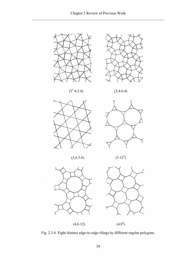
(33.42), (32.4.3.4), (3.4.6.4), (3.6.3.6), (3.122), (44), (4.6.12), (4.82) and (63), see
Figs. 2.3.3 and 2.3.4.

Chapter 2 Review of Previous Work
———————————————————————————————————
38
(36) (44)
(63)
Fig. 2.3.3 The edge-to-edge monohedral tilings by regular polygons.
(34.6) (33.42)
Chapter 2 Review of Previous Work
———————————————————————————————————
39
(32.4.3.4) (3.4.6.4)
(3.6.3.6) (3.122)
(4.6.12) (4.82)
Fig. 2.3.4 Eight distinct edge-to-edge tilings by different regular polygons.

Chapter 2 Review of Previous Work
———————————————————————————————————
40
• k-uniform tilings
An edge-to-edge tiling by regular polygons is called k-uniform if its vertices form
precisely k transitivity classes with respect to the group of symmetries of the tilings. In
other words, the tiling is k-uniform if and only if it is k-isogonal and its tiles are regular
polygons. There exist twenty distinct types of 2-uniform edge-to-edge tilings by regular
polygons, namely: (36;34.6)1, (36;34.6)2, (36;33.42)1, (36;33.42)2, (36;32.4.12), (36;32.4.3.4),
(36;32.62), (34.6;32.62), (33.42; 32.4.3.4)1, (33.42; 32.4.3.4)2, (33.42; 3.4.6.4), (33.42; 44)1,
(33.42;44)2, (32.4.3.4;3.4.6.4), (32.62;3.6.3.6), (3.4.3.12;3.122), (3.42.6;3.4.6.4),
(3.42.6;3.6.3.6)1, (3.42.6;3.6.3.6)2, and (3.4.6.4;4.6.12), where ()1 and ()2 denote two
different arrangements of 2-uniform edge-to-edge tilings. Some of these tilings are
shown in Fig. 2.3.5.
Denote ( )kK as the number of distinct k-uniform tilings. ( ) 111 =K , ( ) 202 =K ,
( ) 393 =K , ( ) 334 =K , ( ) 155 =K , ( ) 106 =K , ( ) 77 =K , and ( ) 0=kK for each 8≥k .
• Equitransitive and edge-transitive tilings
A tiling by regular polygons is equitransitive if each set of mutually congruent tiles
forms one transitivity class. One such tiling is shown in Fig. 2.3.6.

Chapter 2 Review of Previous Work
———————————————————————————————————
41
(36;32.62) (36;32.4.3.4)
(3.4.3.12;3.122)
Fig. 2.3.5 Examples of 2-uniform tilings.
Fig. 2.3.6 An example of equitransitive tilings.

Chapter 2 Review of Previous Work
———————————————————————————————————
42
• Tilings that are not edge-to-edge
The tilings by regular polygons without the requirement that the tiling is edge-to-edge
are considered here. Some examples are shown in Fig. 2.3.7.
Further consideration should be given to patterns with overlapping motifs. One such
example is given in Fig. 2.3.8. The variety of such patterns is restricted by the number
of basic tilings.
2.3.3 Summary - 3 Types of Simplified Tilings
According to the regular and uniform tilings, there are only three ways to cover the
plane with an identical unit. Tiling (36) makes the unit spread in three directions; tiling
(44) makes the unit spread in four directions; tiling (63) makes the unit spread in six
directions. So all the tilings and patterns can be considered as a unit tessellates in one of
these three ways, see Fig. 2.3.9, though within each unit, a repeatable pattern can be
used. This idea is applied in our research to develop a systematic approach in
determining the layout for mobile assemblies.

Chapter 2 Review of Previous Work
———————————————————————————————————
43
Fig. 2.3.7 Tilings that are not edge-to-edge.
Fig. 2.3.8 Pattern with overlapping motifs.
(a) (34.6) (b) (32.4.3.4)

Chapter 2 Review of Previous Work
———————————————————————————————————
44
(c) (3.4.6.4) (d) (3.6.3.6)
(e) (3.4.3.12;3.122) (f) Tiling that are not edge-to-edge
(g) Pattern with overlapping motifs
Fig. 2.3.9 Units, represented by grey dash lines, in tilings and patterns.

45
3
Bennett Linkage and its Networks
3.1 INTRODUCTION
In this chapter, the possibility of building large space deployable structures using the
Bennett linkage as the basic element is investigated. We examine whether the Bennett
linkage can be used to form large structural mechanisms, and if so, whether it is
possible to achieve the highest expansion/packaging ratio.
Before we proceed, a definition is given here. Consider two Bennett linkages, of which
one has lengths and twists 1a , 1b , 1α and 1β , while the other has 2a , 2b , 2α and 2β . If
21 αα = , 21 ββ = (or 21 αα −= , 21 ββ −= )
2
2
1
1
ba
ba
=(3.1.1)
these two Bennett linkages are considered as similar Bennett linkages.
The layout of the chapter is as follows. Section 3.2 presents the method to form a
network of Bennett linkages. The mathematical derivation of the compact folding and
maximum expansion conditions is given in Section 3.3, resulting in an alternative form
of the Bennett linkage. A simple method to build this alternative form is introduced and
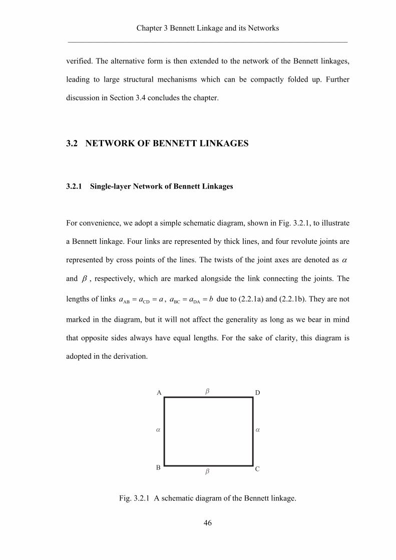
Chapter 3 Bennett Linkage and its Networks
———————————————————————————————————
46
verified. The alternative form is then extended to the network of the Bennett linkages,
leading to large structural mechanisms which can be compactly folded up. Further
discussion in Section 3.4 concludes the chapter.
3.2 NETWORK OF BENNETT LINKAGES
3.2.1 Single-layer Network of Bennett Linkages
For convenience, we adopt a simple schematic diagram, shown in Fig. 3.2.1, to illustrate
a Bennett linkage. Four links are represented by thick lines, and four revolute joints are
represented by cross points of the lines. The twists of the joint axes are denoted as α
and β , respectively, which are marked alongside the link connecting the joints. The
lengths of links aaa == CDAB , baa == DABC due to (2.2.1a) and (2.2.1b). They are not
marked in the diagram, but it will not affect the generality as long as we bear in mind
that opposite sides always have equal lengths. For the sake of clarity, this diagram is
adopted in the derivation.
A D
CB
Fig. 3.2.1 A schematic diagram of the Bennett linkage.

Chapter 3 Bennett Linkage and its Networks
———————————————————————————————————
47
Many such identical Bennett linkages with lengths a , b and twists α , β can be
connected forming a network as shown in Fig. 3.2.2(a). In order to retain the single
degree of mobility, it is necessary to assume that every small 4R linkage in the network
should also be a Bennett linkage. While large Bennett linkage ABCD has lengths a , b
and twists α , β , the smaller Bennett linkages around it, which are marked with
numbers 1 to 8, will have lengths ia , ib and twists iα , iβ (i = 1, 2, ···, 8), see
Fig. 3.2.2(b).
2
D
CB
A1
3
4
5
6
7
8
(a)
D
CB
A
F
E
J
G
I
H
L
K
3
1 1
2 2
2
2
1
1
3
3
3
4
5
8 7
6
5
7
4
4
4
5
5
7
8 8
8
6
6
6
7
(b)Fig. 3.2.2 Single-layer network of Bennett linkages.
(a) A portion of the network; (b) enlarged connection details.

Chapter 3 Bennett Linkage and its Networks
———————————————————————————————————
48
Considering links AB, BC, CD, and DA, we have
aaaa =++ 321 , αααα =++ 321
bbbb =++ 543 , ββββ =++ 543
aaaa =++ 765 , αααα =++ 765
bbbb =++ 187 , ββββ =++ 187
(3.2.1)
Define angles σ , τ , υ and φ as revolute variables shown in Fig. 3.2.2(b). For Bennett
linkage 1, there is
)(21sin
)(21sin
2tan
2tan
11
11
αβ
αβσπυπ
−
+=
−− (3.2.2)
For Bennett linkage 2,
)(21sin
)(21sin
2tan
2tan
22
22
αβ
αβτπσπ
−
+=
−− (3.2.3)
For Bennett linkage 3,
)(21sin
)(21sin
2tan
2tan
33
33
αβ
αβφπτπ
−
+=
−− (3.2.4)
Finally, for Bennett linkage ABCD,
)(21sin
)(21sin
2tan
2tan
αβ
αβφπυπ
−
+=
−− (3.2.5)
Combining (3.2.2) − (3.2.5) gives

Chapter 3 Bennett Linkage and its Networks
———————————————————————————————————
49
)(21sin
)(21sin
)(21sin
)(21sin
)(21sin
)(21sin
)(21sin
)(21sin
22
22
33
33
11
11
αβ
αβ
αβ
αβ
αβ
αβ
αβ
αβ
−
+⋅
−
+=
−
+⋅
−
+(3.2.6)
This is a non-linear equation and many solutions may exist. By observation, two
solutions can be immediately determined, which are
12
12
3
3
ββαα
ββαα
−=−=
==
(3.2.7a)
and
32
32
1
1
ββαα
ββαα
−=−=
==
(3.2.7b)
Similar analysis can be applied to Bennett linkages around links BC, CD and DA, see in
Fig. 3.2.2(a). The twists of Bennett linkages 3, 4 and 5 should therefore satisfy
54
54
3
3
ββαα
ββαα
−=−=
==
(3.2.8a)
or
34
34
5
5
ββαα
ββαα
−=−=
==
(3.2.8b)
The twists of Bennett linkages 5, 6 and 7 should satisfy
56
56
7
7
ββαα
ββαα
−=−=
==
(3.2.9a)
or
76
76
5
5
ββαα
ββαα
−=−=
==
(3.2.9b)

Chapter 3 Bennett Linkage and its Networks
———————————————————————————————————
50
The twists of Bennett linkages 7, 8 and 1 should satisfy
18
18
7
7
ββαα
ββαα
−=−=
==
(3.2.10a)
or
78
78
1
1
ββαα
ββαα
−=−=
==
(3.2.10b)
Combining four sets of solutions (3.2.7) – (3.2.10), two common solutions, which
enable the mobility of the network in Fig. 3.2.2(a), are obtained:
78634251
78634251
βββββββββααααααααα
−==−====−==−====
(3.2.11a)
and
54618273
54618273
βββββββββααααααααα
−==−====−==−====
(3.2.11b)
Because of symmetry, (3.2.11a) and (3.2.11b) are essentially same. Thus, we take only
(3.2.11a) in the derivation next.
Note that, due to (2.2.2), the corresponding lengths of each Bennett linkage should
satisfy
i
i
i
i
ba
ba
===βα
βα
sinsin
sinsin (i = 1, 2, ···, 8) (3.2.12)
A close examination of (3.2.11a) and (3.2.12) reveals the order of distribution of
Bennett linkages within a mobile network. Diagonally from top left corner to bottom

Chapter 3 Bennett Linkage and its Networks
———————————————————————————————————
51
right, there are two types of rows of Bennett linkages, see Fig. 3.2.3. The first type
consists of Bennett linkages with lengths proportional to a and b , and twists being α
and β , which are denoted as ‘I’ in Fig. 3.2.3. The second type, next to the first one, are
made of Bennett linkages with lengths proportional to a and b , and twists being iα
and iβ or iα− and iβ− , which are denoted as ‘IIi’ or ‘-IIi’, respectively, and
ba
i
i =βα
sinsin
A further study has shown that the first row of Bennett linkages in Fig. 3.2.3 can
actually have twists jα and jβ , which may be different from α and β , as long as
ba
j
j =βα
sinsin
If we denote this type of Bennett linkages as ‘Ij’, the arrangement of the mobile network
can be redrawn as that in Fig. 3.2.4, in which a very interesting pattern emerges:
diagonally from top left to bottom right, each row of Bennett linkages belong to the
same type. This leads to an important feature: the joints, which form the diagonal
direction from top left to bottom right, remain along a straight line during deployment.
Therefore, if we draw a set of guidelines in that direction, each of which passes through
a number of joints, these lines remain straight and parallel to each other during
deployment though the distances between the guidelines may vary.
Generally, the network shown in Fig. 3.2.4 deploys into a cylindrical profile. The joints
forming those parallel guidelines remain straight. They expand along the longitudinal

Chapter 3 Bennett Linkage and its Networks
———————————————————————————————————
52
direction of the cylinder. In the other diagonal direction, joints generally deploy spirally
on the surface of the cylinder, see Fig. 3.2.5.
II2
II4
I
I
I
I
I
I
I
I
I
I
I
I
I
II2
-II2
-II2
II2
II1
II3
II3
-II3
II3
-II3
Fig. 3.2.3 Network of Bennett linkages with the same twists.
II1
I1
I1
I1
I2
-II2
II2
II2
II2
-II2
I2
I2
I2
I2
I2
I2
II3
II4
-II3
II3
-II3 I3
I3
I3
Fig. 3.2.4 Network of similar Bennett linkages with guidelines.

Chapter 3 Bennett Linkage and its Networks
———————————————————————————————————
53
(a) (b)
(c) (d)
Fig. 3.2.5 A special case of single-layer network of Bennett linkages.
(a) – (c) Deployment sequence; (d) view of cross section of network.
The curvature of the cylinder inscribed the network depends on the values of the lengths
and twists of links of each Bennett linkage and the deployment angle of the network.
For instance, for the model shown in Fig. 3.2.5, where the lengths and twists of the links
are
3aai = ,
3bbi = (i = 1, 2, ···, 8)
ααααααααα ==−====−== 87654321
βββββββββ ==−====−== 87654321
the radius of its deployed cylinder, which is inscribed the network, is

Chapter 3 Bennett Linkage and its Networks
———————————————————————————————————
54
atttt
tR ⋅
+
+++−
++=
ϕθϕθ
θθ
coscoscoscos121
cos21sin 2
2
where abt = , θ and ϕ are deployment angles related by (2.2.6).
When 4πα = , the relationship between deployment angle θ and unit radius aR / is
shown in Fig. 3.2.6.
During deployment, the network expands in the helical direction on the surface of the
cylindrical profile. In the special case where the link lengths are the same, i.e. ba = ,
the network expands only in the circumferential direction, forming a circular arch as
shown in Fig. 3.2.7. In another special case where the twists are αααα ==−= 321 and
ββββ ==−= 321 , the network remains completely flat during the deployment, see
Fig. 3.2.8.
0
1
2
3
4
5
6
R/a
/2/4 /43
t=1
t=0.8
t=0.67
t=0.5
Fig. 3.2.6 aR / vs θ for different t ( abt /= ).

Chapter 3 Bennett Linkage and its Networks
———————————————————————————————————
55
(a)
(b)
(c)
Fig. 3.2.7 (a) – (c) Deployment sequence of a deployable arch.

Chapter 3 Bennett Linkage and its Networks
———————————————————————————————————
56
(a)
(b)
(c)
Fig. 3.2.8 (a) – (c) Deployment sequence of a flat deployable structure.

Chapter 3 Bennett Linkage and its Networks
———————————————————————————————————
57
3.2.2 Multi-layer Network of Bennett linkages
The network of Bennett linkages presented so far does not have over-lapping layers. A
typical basic unit of single-layer network of Bennett linkages can be taken from
Fig. 3.2.4 and redrawn as Fig. 3.2.9(a). The twists are marked alongside each link.
E
D
B C
A
G
I
J
K L
M
N
PQ
S
V
3
3
3
7
3
7
7
7
D
B C
A
J
K
N
P
S
VR
T
3
3
7
7
0
0 0
0
(a) (b)
E
D
B C
A
G
I
L
M
Q
F
HE
D
B C
A
G
I
J
K L
M
N
PQ
S
V
F
H
R
T
3
3
3
7
3
7
7
7
(c) (d)
Fig. 3.2.9 A basic unit of Bennett linkages.
(a) A basic unit of single-layer network; (b) part of multi-layer unit;
(c) the other part; (d) a basic unit of multi-layer network.

Chapter 3 Bennett Linkage and its Networks
———————————————————————————————————
58
Now let us examine whether the top right small Bennett linkage PVND can be
connected with the bottom left one JBKS while retaining mobility, see Fig. 3.2.9(b).
This can only be possible if and only if all the rectangular loops are Bennett linkages.
The deployment angles and twists for each of the loops are shown in Fig. 3.2.9(b). Note
that πφτ =+ . Thus, the following relationships can be found.
For ABCD,
)(21sin
)(21sin
2tan
2tan
αβ
αβσπυπ
−
+=
−− (3.2.13)
For JBKS,
)(21sin
)(21sin
2tan
2tan
33
33
αβ
αβτπυπ
−
+=
−− (3.2.14)
For PVND,
)(21sin
)(21sin
2tan
2tan
77
77
αβ
αβτπυπ
−
+=
−− (3.2.15)
For RSTV,
)(21sin
)(21sin
2tan
2tan
00
00
αβ
αβσπυπ
−
+=
−− (3.2.16)
For AJTP with twists 70 αα + , 30 ββ + , and variables φπ − , σπ − ,
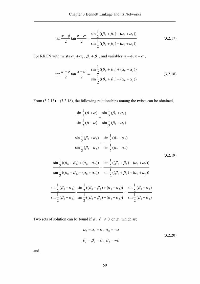
Chapter 3 Bennett Linkage and its Networks
———————————————————————————————————
59
))()((21sin
))()((21sin
2tan
2tan
7030
7030
ααββ
ααββσπφπ
+−+
+++=
−− (3.2.17)
For RKCN with twists 30 αα + , 70 ββ + , and variables φπ − , σπ − ,
))()((21sin
))()((21sin
2tan
2tan
3070
3070
ααββ
ααββσπφπ
+−+
+++=
−− (3.2.18)
From (3.2.13) – (3.2.18), the following relationships among the twists can be obtained,
)(21sin
)(21sin
)(21sin
)(21sin
00
00
αβ
αβ
αβ
αβ
−
+=
−
+
)(21sin
)(21sin
)(21sin
)(21sin
77
77
33
33
αβ
αβ
αβ
αβ
−
+=
−
+
))()((21sin
))()((21sin
))()((21sin
))()((21sin
3070
3070
7030
7030
ααββ
ααββ
ααββ
ααββ
+−+
+++=
+−+
+++
)(21sin
)(21sin
))()((21sin
))()((21sin
)(21sin
)(21sin
00
00
3070
3070
33
33
αβ
αβ
ααββ
ααββ
αβ
αβ
−
+=
+−+
+++⋅
−
+
(3.2.19)
Two sets of solution can be found if α , β ≠ 0 or π , which are
ααα == 73 , αα −=0
βββ == 73 , ββ −=0
(3.2.20)
and

Chapter 3 Bennett Linkage and its Networks
———————————————————————————————————
60
073 == αα , αα =0
073 == ββ , ββ =0
(3.2.21)
When α , β = 0 or π , the network becomes a number of overlapped planar crossed
isograms or planar parallelograms.
Denote the lengths of links for small Bennett linkages JBKS, PVND, and RSTV as 3a ,
3b , 7a , 7b and 0a , 0b . Obviously,
ba
ba
ba
ba
===0
0
7
7
3
3 (3.2.22a)
bbbb
aaaa
=++
=++
703
703
(3.2.22b)
The solutions given in (3.2.20) can be easily applied to connect the top left Bennett
linkage AQEI and the bottom right one GMCL, see Fig. 3.2.9(c). Doing so, we are able
to create a multi-layer connection as shown in Fig. 3.2.9(d). When the twists of both
parts are (3.2.20) or (3.2.21), the profile of network is flat. When the twists of one part
are (3.2.20) and those of the other are (3.2.21), the network forms a curved profile.
The current arrangement can be extended by repetition. For example, links in one of the
central smaller Bennett linkages shown in Fig. 3.2.9(d) can be extended and connected
again to another Bennett linkage similar to ABCD but on a different layer. This process
will not affect the mobility of the entire assembly. A model of such multi-layer structure
is shown in Fig. 3.2.10.
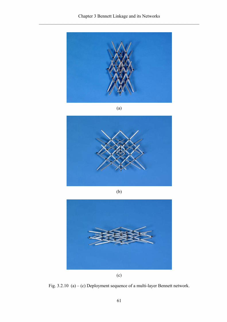
Chapter 3 Bennett Linkage and its Networks
———————————————————————————————————
61
(a)
(b)
(c)
Fig. 3.2.10 (a) – (c) Deployment sequence of a multi-layer Bennett network.

Chapter 3 Bennett Linkage and its Networks
———————————————————————————————————
62
3.2.3 Connectivity of Bennett Linkages
Baker and Hu (1986) attempted to connect two similar Bennett linkages together with
only revolute joints, see Fig. 3.2.11. They found that the assembly lost mobility, i.e. it
becomes a rigid structure.
In this section, we intend to show that, based on the work presented in previous
sections, the mobility of the assembly can be retained if two Bennett linkages are
connected by a type of Bennett connection. Note that the Bennett connection is different
from the Bennett joint described in Section 2.2.3 (page 32).
Let us start with the structure shown in Fig. 3.2.12(a), which is based on the solution
given in (3.2.21), in which loops AJSP and RKCN are Bennett linkages similar to
Bennett linkage ABCD. If the lengths for ABCD are a and b , then loop AJSP has
lengths of ak1 and bk1 , while loop RKCN has lengths of ak2 and bk2 .
Fig. 3.2.11 Connection of two similar Bennett linkages by four revolute joints
at locations marked by arrows.

Chapter 3 Bennett Linkage and its Networks
———————————————————————————————————
63
We can also create a complementary set of extensions as sketched in dash lines in
Fig. 3.2.12(b). Again loops IBLH and QFMD are Bennett linkages similar to ABCD,
whose lengths are proportional to those of ABCD with ratios 3k and 4k , respectively.
CB K
N
S
A D
J
P
R
0
0
0
0
0
0
0
0
CB LK
N
S
A D
I
J M
PQ
F
H
0
0
0
0
0
0
0
0
ER
(a) (b)
CB LK
N
X
A D
I
J M
PQ
W
U
V
CB LK
N
X Y
A D
I
J M
PQ
W Z
U
V
E
T
(c) (d)
Fig. 3.2.12 Connection of two Bennett linkages ABCD and WXYZ.
(a) Addition of four bars; (b) a complementary set;
(c) further extension; (d) formation of the inner Bennett linkage.

Chapter 3 Bennett Linkage and its Networks
———————————————————————————————————
64
Then the lengths of section IJ, MN, KL and PQ are
bkka
bkka
akka
akka
)1(
)1(
)1(
)1(
41PQ
32KL
42MN
31IJ
−+=
−+=
−+=
−+=
(3.2.23)
Now introduce bar WX by connecting it to the existing structure at U and V using
revolute joints, see Fig. 3.2.12(c). To ensure connectivity without the loss of mobility,
loop IJVU must be a Bennett linkage similar to ABCD. Thus, there must be
bkkaa
akkaa
)1(
)1(
31JVIU
31IJUV
−+==
−+==(3.2.24)
while the twists are α and β , respectively.
The same can be done to the remaining sides of the structure, see Fig. 3.2.12(d). Again,
to retain mobility, all of the rectangular loops, except those with zero twists such as
AIEQ, must be Bennett linkages similar to ABCD. Based on this requirement, the twists
marked alongside each link in Fig. 3.2.12(d) should be adopted. Loop WXYZ also
becomes a Bennett linkage similar to ABCD with
bkkkkaa
akkkkaa
)3(
)3(
4321XYWZ
4321YZWX
−−−−==
−−−−==(3.2.25)
and the twists α− and β− , respectively.
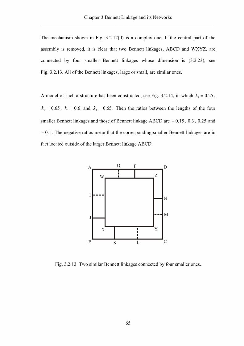
Chapter 3 Bennett Linkage and its Networks
———————————————————————————————————
65
The mechanism shown in Fig. 3.2.12(d) is a complex one. If the central part of the
assembly is removed, it is clear that two Bennett linkages, ABCD and WXYZ, are
connected by four smaller Bennett linkages whose dimension is (3.2.23), see
Fig. 3.2.13. All of the Bennett linkages, large or small, are similar ones.
A model of such a structure has been constructed, see Fig. 3.2.14, in which 25.01 =k ,
65.02 =k , 6.03 =k and 65.04 =k . Then the ratios between the lengths of the four
smaller Bennett linkages and those of Bennett linkage ABCD are 15.0− , 3.0 , 25.0 and
1.0− . The negative ratios mean that the corresponding smaller Bennett linkages are in
fact located outside of the larger Bennett linkage ABCD.
CB LK
N
X Y
A D
I
J M
PQ
W Z
U
V
E
T
Fig. 3.2.13 Two similar Bennett linkages connected by four smaller ones.

Chapter 3 Bennett Linkage and its Networks
———————————————————————————————————
66
(a)
(b)
(c)
Fig. 3.2.14 (a) – (c) Three configurations of connection of two similar Bennett linkages.

Chapter 3 Bennett Linkage and its Networks
———————————————————————————————————
67
(3.2.25) also determines the size of the inner Bennett linkage. Obviously, when
24321 =+++ kkkk , the inner Bennett linkage becomes identical in size to the outer
one. From (3.2.23), when 21 kk = , 43 kk = and 131 =+ kk , the size of the four smaller
connection Bennett linkages reduces to zero. We define this type of zero-sized Bennett
linkages as the Bennett connection. The key difference between a Bennett connection
and a conventional revolute joint is the relative motions of the pair of links connected.
The links remain co-planar when connected with a conventional revolute joint, which is
not true when connected by a Bennett connection. The discovery presented here actually
indirectly confirms that Baker and Hu’s assembly is rigid.
3.3 ALTERNATIVE FORM OF BENNETT LINKAGE
3.3.1 Alternative Form of Bennett Linkage
For the Bennett linkage shown in Fig. 3.3.1, (2.2.6) indicates that ϕ must be close to π
while θ approaches 0, or vice versa, which means that the distance between B and D
become smallest while that between A and C is largest. As a result, the Bennett linkage
cannot be folded completely in both directions simultaneously. However, we are to
demonstrate in this section that modification can be carried out to make compact folding
possible.
For the purpose of geometric derivation, the joints of Bennett linkage are marked with
letters, i.e. A, B, C, etc. So the lengths and twists of linkage are also marked with letters
in the subscripts. For instance, ABα is the twist between joint A and joint B.

Chapter 3 Bennett Linkage and its Networks
———————————————————————————————————
68
Figure 3.3.2(a) shows an equilateral special case of Bennett linkage, where
laaaa ==== DACDBCAB (3.3.1)
ααα == CDAB
απαα −== DABC
(3.3.2)
This linkage is symmetric about both the plane through AC and perpendicular BD and
the plane through BD and perpendicular AC even though lines AC and BD may not
cross each other. The axes of revolute joints are marked as dash-dot lines at A, B, C and
D. The positive directions of the axes are also shown.
Denote M and N as the respective middle points of BD and AC, see Fig. 3.3.2(b).
Obviously, ∆ABD and ∆CDB are isosceles and identical triangles due to (3.3.1). So are
∆BCA and ∆DAC. These lead to the conclusion that ∆AMC and ∆BND are both
isosceles triangles. Hence MN is perpendicular to both AC and BD. Furthermore,
extensions of the axes of revolute joints must meet with the extension of MN at P and
Q, respectively, due to symmetry.
A
B
C
D
2 -
2 -
Fig. 3.3.1 A Bennett linkage.

Chapter 3 Bennett Linkage and its Networks
———————————————————————————————————
69
A
B
C
D
2 -
2 -
(a)
A
B
C
D
E
F
G
H
N
M
P
Q
(b)
A
B
C
D
E
F
G
H
N
M
P
Q
ST
(c)
Fig. 3.3.2 Equilateral Bennett linkage. Certain new lines are introduced in (a), (b) and
(c) for derivation of compact folding and maximum expansion conditions.

Chapter 3 Bennett Linkage and its Networks
———————————————————————————————————
70
Consider now four alternative connection points E, F, G and H along the extensions of
the revolute axes AP, BQ, CP and DQ, respectively. To preserve symmetry, define
c== AEGC
d== DHBF
Hence,
)cos(2EF AB2222
απ −−++= cddcl
BC2222
cos2FG αcddcl −++=(3.3.3)
Substituting (3.3.2) into (3.3.3) gives
αcos2FGEF 222 cddcl +++== (3.3.4)
Similarly,
HEGHFGEF === (3.3.5)
which means EFGH is also equilateral.
For any given Bennett linkage ABCD, (3.3.4) and (3.3.5) show that EF, FG, GH and HE
have constant length provided that both c and d are given. They do not vary with the
revolute variables, θ and ϕ . Thus, it is possible to replace EF, FG, GH and HE with
bars connected by the revolute joints whose axes are along BF, CG, DH and AE,
respectively. EFGH is therefore an alternative form of the Bennett linkage ABCD.
For each given set of c and d , an alternative form for the Bennett linkage can be
obtained. The next step is to examine if a particular form would provide the most
compact folding.

Chapter 3 Bennett Linkage and its Networks
———————————————————————————————————
71
When the linkage in the alternative form displaces, the distance between E and G varies.
So does the distance between F and H. Assume that when the structure is fully folded,
deployment angles θ and ϕ become fθ and fϕ , respectively. The condition for the
most compact folding is
0FHEG == (3.3.6)
This means that physically the mechanism becomes a bundle.
(3.3.6) can be written in term of c , d and the deployment angles, which is done next.
Consider ∆ADC in Fig. 3.3.2(b). It can be found that
)cos1(2)cos(CDAD2CDADAC 2222ϕϕπ +=−⋅−+= l (3.3.7)
Similarly, in ∆ABD, there is
)cos1(2)cos(ADAB2ADABBD 2222θθπ +=−⋅−+= l (3.3.8)
while in ∆BCM,
)cos1(2
BMBCCM2222
θ−=−=l (3.3.9)
Thus, from ∆AMC,
θϕ
cos1cos121AMCcos
−+
−=∠ (3.3.10)
From quadrilateral PAMC,
1cos1cos12AMCcosAPCcos −
−+
=∠−=∠θϕ (3.3.11)
Because in ∆APC,
θϕθ
cos1coscosPC4APC)cos(1PC2AC
222
−−−
=∠−= (3.3.12)

Chapter 3 Bennett Linkage and its Networks
———————————————————————————————————
72
Comparing (3.3.7) with (3.3.12) yields
)cos(cos2)cos1)(cos1(PC 22
θϕθϕ
+−−+
= l (3.3.13)
Similarly it can be obtained that
)cos(cos2)cos1)(cos1(QB 22
θϕϕθ
+−−+
= l (3.3.14)
In ∆EPG, there is
θϕθ
cos1coscos)PC(4)APCcos1()PC(2EG 222
−−−
+=∠−+= cc (3.3.15)
and similarly
ϕϕθ
cos1coscos)QB(4)BQDcos1()QB(2FH 222
−−−
+=∠−+= dd (3.3.16)
In general, APC∠ and BQD∠ cannot reach zero at the same time. Substituting
(3.3.15) and (3.3.16) into (3.3.6) yields
)cos(cos2)cos1)(cos1(
PCff
fflcθϕθϕ
+−
−+−=−=
)cos(cos2)cos1)(cos1(
QBff
ffldθϕ
θϕ+−
+−−=−=
(3.3.17)
The above equations show how the values of c and d are related to the fully folded
deployment angles fθ and fϕ . In fact, c and d can be determined graphically as
solutions (3.3.17) simply mean that E and G should move to a single point P, and F and
H go to Q if the configuration shown Fig. 3.3.2(b) represents the fully folded

Chapter 3 Bennett Linkage and its Networks
———————————————————————————————————
73
configuration of linkage EFGH. In this case, positive values of c and d will be used in
the following derivation. Thus, (3.3.17) becomes
)cos(cos2)cos1)(cos1(
ff
fflcθϕ
θϕ+−
−+=
)cos(cos2)cos1)(cos1(
ff
ffldθϕθϕ
+−+−
=
(3.3.18)
Having obtained the linkage corresponding to the most efficient folding configuration,
what is the form of Bennett linkage that covers the largest area? To answer this
question, it is necessary to find out the geometrical condition relating to the maximum
coverage.
Figure 3.3.2(c) shows the alternative form of the Bennett linkage EFGH. Due to
symmetry, a line between E with G will intersect MN at T, and that between F and H
will intersect MN at S. The projection of EFGH will cover a maximum area if
0ST = (3.3.19)
when deployment angles reach dθ and dϕ . This implies that EFGH is completely
flattened to a rhombus.
Again, ST can be expressed in term of c , d and deployment angles.
Based on (3.3.7) and (3.3.9),
)cos(cos24
ACCMCNCMMN22
2222ϕθ +−=−=−=
l (3.3.20)

Chapter 3 Bennett Linkage and its Networks
———————————————————————————————————
74
Considering (3.3.11) gives
2sin
2cos
)APC21
2sin(PGEsin
θ
ϕπ
=∠−=∠
So,
2sin
2cos
PGEsinNTθ
ϕ
⋅=∠⋅= cc (3.3.21)
Similarly,
2sin
2cos
QFHsinMSϕ
θ
⋅=∠⋅= dd (3.3.22)
Hence, considering (3.3.20), (3.3.21) and (3.3.22), ST can be written as
2sin
2cos
2sin
2cos
2)cos(cosNTMSMNST
θ
ϕ
ϕ
θϕθ cdl −−
+−=−−= (3.3.23)
When dθθ = and dϕϕ = ,
0
2sin
2cos
2sin
2cos
2)cos(cosST =−−
+−=
d
d
d
d
dd cdlθ
ϕ
ϕ
θϕθ (3.3.24)
due to (3.3.19).
Substituting c and d obtained from (3.3.18) into (3.3.24) and considering

Chapter 3 Bennett Linkage and its Networks
———————————————————————————————————
75
αϕθϕθ
cos1
2tan
2tan
2tan
2tan == ffdd (3.3.25)
we have
2222224 tan
2sec
2sec
2tan
2tantan
+= α
θθθθα fdfd (3.3.26)
If πθ ≤≤ f0 , then πθπ 2≤≤ d . (3.3.26) becomes
αθθθθα 2222 tan2
sec2
sec2
tan2
tantan +=− fdfd (3.3.27)
Solutions to (3.3.27) only exist when the value of α is in the range between
)3/1arccos( and )3/1arccos(−π , i.e., 70.53° to 109.47°. Within this range, the
relationship between dθ and fθ for a set of given α is shown in Fig. 3.3.3. Note that
in most circumstances, each fθ corresponds to two values of dθ . This means that there
are two possible deployed configurations in which the structure built using the
alternative forms of the Bennett linkage can be flattened. For )3/1arccos(<α or
)3/1arccos(−> πα , there is no pair of fθ and dθ satisfying (3.3.27). Therefore the
structure is incapable of being flattened despite that it can be folded up compactly, or
vice versa.
From (3.3.4), the actual side length of the alternative form of the Bennett linkage, L ,
can be obtained as
αcos2222 cddclL +++= (3.3.28)
Substituting (3.3.18) into (3.3.28), we have

Chapter 3 Bennett Linkage and its Networks
———————————————————————————————————
76
fflL
ϕθ coscos2+
−= (3.3.29)
Figure 3.3.4 shows the relationship between fθ and lL / , lc / , ld / when 12/7πα = .
0 f/3 /32
2
/34
/35
d
/127=
/3619=/95=
/53=−arccos(1/3)=
Fig. 3.3.3 dθ vs fθ for a set of given α .
0
1
2
L/l
c/l
d/l
f/32/3
Fig. 3.3.4 lL / , lc / and ld / vs fθ when 12/7πα = .

Chapter 3 Bennett Linkage and its Networks
———————————————————————————————————
77
Denote δ as the angle between two adjacent sides of the alternative form of the Bennett
linkage in its flattened configuration when dθθ = , dϕϕ = . Thus, FGH∠=δ when S
and T in Fig. 3.3.2(c) become one point. We have
EGFH
EG21
FH21
2tan ==
δ
Expressing FH and EG in terms of angles gives
−−
⋅
+−−+
++−
−+
+−+−
++−
+−
=d
d
dd
dd
ff
ff
dd
dd
ff
ff
ϕθ
θϕθϕ
θϕθϕ
θϕθϕ
θϕθϕ
δcos1cos1
)cos(cos2)cos1)(cos1(
)cos(cos2)cos1)(cos1(
)cos(cos2)cos1)(cos1(
)cos(cos2)cos1)(cos1(
arctan2
(3.3.30)
This relationship is plotted in Fig. 3.3.5 when 12/7πα = . Similar to relationship
between dθ and fθ , there are two values of δ for each fθ .
f/32
/32
/3
/3
/9
Fig. 3.3.5 δ vs fθ when 12/7πα = .

Chapter 3 Bennett Linkage and its Networks
———————————————————————————————————
78
It is interesting to note that among the rhombuses with the same side-length, the square
has the largest area, i.e.,
2πδ = (3.3.31)
Considering (3.3.30), (3.3.31) becomes
)cos1()cos(cos
)cos(cos2)cos1)(cos1(
)cos(cos2)cos1)(cos1(
)cos1()cos(cos
)cos(cos2)cos1)(cos1(
)cos(cos2)cos1)(cos1(
2
2
d
dd
dd
dd
ff
ff
d
dd
dd
dd
ff
ff
ϕθϕ
θϕθϕ
θϕθϕ
θθϕ
θϕθϕ
θϕθϕ
−+−
+−+−
++−
+−
=−
+−
+−−+
++−
−+
(3.3.32)
Considering (3.3.25), (3.3.32) can be simplified as
αθθθ 2222 sec2
tan2
sec2
tan += ddf (3.3.33)
So when α , dθ and fθ satisfy both of (3.3.27) and (3.3.33), the fully deployed
configuration of alternative form of the Bennett linkage is a square.
Solving (3.3.27) and (3.3.33), we obtain,
fd θθ 2=
)12
(tansectan 222 −= ff
θθα
This relationship is shown in Fig. 3.3.6, which is in fact the projection of the intersected
curve between the surface of (3.3.27) and that of (3.3.33).

Chapter 3 Bennett Linkage and its Networks
———————————————————————————————————
79
Also, very interestingly, for any square fully deployed configuration, we always have
lL 2= (3.3.34)
due to (3.3.27), (3.3.29) and (3.3.33).
Finally, we like to point out that normally, for a given α , there are two sets of dθ and
fθ , in which configuration of the corresponding alternative form of Bennett linkage is
square. However, when
31arccos=α or
31arccos−π ,
there is only one solution,
πθ32
=f and πθ34
=d .
In this case,
ldc46
== , lL 2= .
f/65/2 /32
/95
/1811
Fig. 3.3.6 α vs fθ when the fully deployed structure based on the alternative form of
the Bennett linkage forms a square.

Chapter 3 Bennett Linkage and its Networks
———————————————————————————————————
80
3.3.2 Manufacture of Alternative Form of Bennett linkage
According to Crawford et al. (1973), for a close loop consisting n bars with identical
cross-section, the cross-section of the whole structure in the folded configuration should
be n regular polygon in order to achieve the most compact folding. So for the alternative
form of Bennett linkage, each link could be made of bars with square cross-section.
Pellegrino et al. (2000) revealed a model of 4R linkage which is in fact an alternative
form of the Bennett linkage. Figure 3.3.7 shows such a model though angle ω in the
reported model was 4/π in the fully deployed configuration. This particular example
shows that construction of a Bennett linkage with compact folding and maximum
expansion is not only mathematically feasible, as we proved in the previous section, but
also practically possible.
A
A
A-section
Position of hinges
L
Fig. 3.3.7 The alternative form of Bennett linkage made from square cross-section bars
in the deployed and folded configurations.

Chapter 3 Bennett Linkage and its Networks
———————————————————————————————————
81
In general, the model shown in Fig. 3.3.7 has three design parameters: L , λ and ω .
The number matches that presented in the previous section in which the geometric
parameters are l , α , c (or d ). In this section, we will establish the relationships among
two sets of parameters.
Figure 3.3.8 shows a fully deployed linkage EFGH which is the alternative form of the
Bennett linkage. The linkage has reached its maximum expansion and thus, EFGH
becomes a plane rhombus. For simplification in description, let us define a coordinate
system where axis x passes through FH and axis y through EG. The linkage EFGH is
therefore symmetric about both xoz and yoz planes where o is the centre of EFGH and
axis z is perpendicular to plane xoy. Now introduce a square bar, shown in grey colour
in Fig. 3.3.8 to replace link FG in such a way that one of the edges of the square bar lies
along FG. The bar is terminated by planes GIJK and FUVW, created by slicing the bar
by the plane yoz and xoz, respectively.
E
H
o
z
Q
F
G
KJ
W
VU
Id
d
x
P
y
Fig. 3.3.8 The alternative form of Bennett linkage with square cross-section bars in
deployed configuration.

Chapter 3 Bennett Linkage and its Networks
———————————————————————————————————
82
An enlarged diagram of bar FG is shown in Fig. 3.3.9(a), in which GI and FU are the
axes of the revolute joints. Plane x'o'y' is through JV and parallel to plane xoy. A typical
square cross-section is marked as RXYZ. The projection of the bar is given in
Fig. 3.3.9(b), in which X′, R′ and Z′, etc. represent the projection of X, R and Z on the
plane x'o'y', etc.
Assume
1ZRYZXYRX ====
The following relationships can be obtained from Fig. 3.3.9(b).
λcos1ZRYX ⋅=′′=′
λsin1ZYRX ⋅=′=′′
)cos(sin1ZX λλ +⋅=′′
λsin1WWXXII ⋅=′=′=′
λcos1UUZZKK ⋅=′=′=′
ωλ
ω coscos
cosZRWVUF =
′′=′=′′
ωλ
ω cossin
cosRXVUWF =
′′=′=′′
ωλ
ω sincos
sinZRJIKG =
′′=′=′′
ωλ
ω sinsin
sinRXKJIG =
′′=′=′′

Chapter 3 Bennett Linkage and its Networks
———————————————————————————————————
83
So we have
λωλ 2
2
222cos
sinsinKKKJJKGI +=′+′== (3.3.35)
λωλ 2
2
222sin
coscosWWWVVWFU +=′+′== (3.3.36)
R
Y
ZX
F
GK
J
M
I
V
Wz
U
d
d
f
f
o’x’
y’
(a)
R
Z’
X
M’
YX’ R’
W’
F’U’
V
Z’Y
X’R’
K’G’I’ J
L
o’
x’
y’
(b)
Fig. 3.3.9 The geometry of the square cross-section bar.
(a) In 3D; (b) projection on the plane x'o'y' and the cross section RXYZ.

Chapter 3 Bennett Linkage and its Networks
———————————————————————————————————
84
Let us now draw line FM parallel to GI and cross IW at M. Thus,
α=∠MFU
and
FUFM2UMFUFMcos
222
⋅⋅−+
=α (3.3.37)
Because of FM // GI and FG // MI, we have
λωλ 2
2
2
cossinsinGIFM +== (3.3.38)
ωλ
sinsinIGMF =′′=′′ (3.3.39)
and F′M′ ⊥ W′U′.
Then,
222UFMFMU ′′+′′=′′ (3.3.40)
and
222)UUMM(MUUM ′−′+′′= (3.3.41)
Substituting (3.3.36), (3.3.38) and (3.3.41) into (3.3.37), we obtain
( )ωλωλωλα
2cos2cos182sin2sin2sin2sincos
22 −+±= (3.3.42)
(3.3.42) is the relationship between design parameters ω , λ and twist α of the original
Bennett linkage, which is plotted in Fig. 3.3.10 for a set of given α . It is interesting to
note that, for 2/0 πλ ≤≤ and 2/0 πω ≤≤ , the range of α is between )3/1arccos(
and )3/1arccos(−π , which is the same as that obtained from (3.3.27).

Chapter 3 Bennett Linkage and its Networks
———————————————————————————————————
85
0 /2
/2
/4
/4 /127=
/3619=/95=
/53=−arccos(1/3)=
Fig. 3.3.10 λ vs ω for a set of given α .
Our next step is to obtain the relationship among λ , ω and dθ , dϕ , fθ , fϕ .
As described in (3.3.11), in deployed configuration,
1cos1cos12EPGcos −
−+
=∠d
d
θϕ
1cos1cos12FQHcos −
−+
=∠d
d
ϕθ
(3.3.43)
From Fig. 3.3.8,
dξπ 2EPG −=∠
dγπ 2FQH −=∠(3.3.44)
From Fig. 3.3.9(a),

Chapter 3 Bennett Linkage and its Networks
———————————————————————————————————
86
ωλλξ
sinsincos
KJKKtan =
′′
=d
ωλλγcoscos
sinWVWWtan =
′′
=d
(3.3.45)
From (3.3.43) – (3.3.45), we can obtain that
)2cos2cos1(4)2cos32cos42cos4(cos)14(coscos
λωωλωλλθ
−+−+−
=d (3.3.46a)
)2cos2cos1(4)2cos32cos42cos4(cos)14(coscos
λωωλωλλϕ
−+−−−
=d (3.3.46b)
When the linkage is folded up, EFGH becomes a bundle ST, so does the square cross-
section bars. Bar EF is shown Fig. 3.3.11 in grey colour.
(E,G)
(F, H)S
T
WV
U
K
JI f
f
o
z
x
y
A
B
C
D
Fig. 3.3.11 The alternative form of Bennett linkage with square cross-section bars in
folded configuration.

Chapter 3 Bennett Linkage and its Networks
———————————————————————————————————
87
Similarly to (3.3.43), in folded configuration, we have
1cos1cos1
2ATCcos −−
+=∠
f
f
θϕ
1cos1cos1
2BSDcos −−
+=∠
f
f
ϕθ
(3.3.47)
From Fig. 3.3.11,
fξ2ATC =∠
fγ2BSD =∠(3.3.48)
From Fig. 3.3.9,
λω
ωξ
sintan
tan/XRRX
RGXIRXtan =
′′=
−=f
ωλωγ
tancos1
tanZRRZ
UZRFRZtan =
′′=
−=f
(3.3.49)
From (3.3.47) – (3.3.49), we can obtain that
)2cos2cos1(4)2cos32cos42cos4(cos)14(coscos
λωλωλωωθ
−+−+−
=f (3.3.50a)
)2cos2cos1(4)2cos32cos42cos4(cos)14(coscos
λωλωλωωϕ
−+−−−
=f (3.3.50b)
Now we can get the relationship among λ , ω and lL / , lc / , ld / .
Substituting (3.3.50) into (3.3.29) yields
ωλω
4cos12cos2cos12
−−
=lL (3.3.51)

Chapter 3 Bennett Linkage and its Networks
———————————————————————————————————
88
When the deployed configuration of the alternative form is square, that is 4πω = ,
(3.3.51) gives
2=lL
which is the same as (3.3.34).
Substituting (3.3.50) into (3.3.18) yields
λωωλλω
ωωλ
2222
222
cossincossinsinsin1
cossincos
+−
=lc
λωωλλω
ωωλ
2222
222
cossincossincoscos1
sincossin
+−
=ld
(3.3.52)
Obviously, α , dθ , and fθ from (3.3.42), (3.3.46a), and (3.3.50a) satisfy (3.3.27).
So a set of equations have been obtained relating geometric parameters of an alternative
form of Bennett linkage to the design parameters, based on which a model consisting of
four square cross-section bars can be installed together with hinges as described in
Fig. 3.3.7. The linkage has only one degree of mobility and can be folded into a
compact bundle and deployed into a rhombus. In practice, it is not necessary to know
the characteristics of the original Bennett linkage l , α , and extended distance on the
axes of joints c (or d ). The design work can be done based on the values of L , λ and
ω , though it is much more convenient to use l , α and c (or d ) when analysing the
kinematic behaviour of the linkage such as dθ , dϕ , fθ and fϕ . Several models have
been made which are shown in Figs. 3.3.12 – 3.3.15.

Chapter 3 Bennett Linkage and its Networks
———————————————————————————————————
89
Fig. 3.3.12 Model that 6/πλ = and 180/53πω = .

Chapter 3 Bennett Linkage and its Networks
———————————————————————————————————
90
Fig. 3.3.13 Model that 6/πλ = and 4/πω = .

Chapter 3 Bennett Linkage and its Networks
———————————————————————————————————
91
Fig. 3.3.14 Model that 4/πλ = and 4/πω = .

Chapter 3 Bennett Linkage and its Networks
———————————————————————————————————
92
Fig. 3.3.15 Model that 4/πλ = and 3/πω = .

Chapter 3 Bennett Linkage and its Networks
———————————————————————————————————
93
3.3.3 Network of Alternative Form of Bennett Linkage
Similar to the original Bennett linkage, the alternative form of Bennett linkage can also
form a network with the same layout. The model shown in Fig. 3.3.16 is the alternative
form of the model in Fig. 3.2.8.
3.4 CONCLUSION AND DISCUSSION
This chapter has presented the first attempt to construct a large overconstrained
structural mechanism using Bennett linkages as basic elements. The proposed
mechanisms have the following features.
1. The mechanisms have single degree of mobility and therefore can be controlled with
ease.
2. Only simple revolute joints are required, which means that the mechanisms can be
made without much difficulty and furthermore it increases the reliability of the
mechanisms.
3. They are very rigid as the Bennett linkage itself is geometrically overconstrained
while the method to constructing the networks of Bennett linkages proposed here
add further constraints.

Chapter 3 Bennett Linkage and its Networks
———————————————————————————————————
94
Fig. 3.3.16 Network of alternative form of Bennett linkage.

Chapter 3 Bennett Linkage and its Networks
———————————————————————————————————
95
Firstly, the method to construct networks from original Bennett linkage has been
derived. The basic layout can be considered as criteria to extend the network
unlimitedly. There is a family of networks of Bennett linkages to form single-layer
deployable structures, which in general deploy into profiles of cylindrical surface.
Meanwhile, two special cases of the single-layer structures can be extended to construct
multi-layer structural mechanism. One of them forms a planar profile, whereas the other
forms a curved profile. According to this derivation, a Bennett connection is introduced
to solve the problem to connect two similar Bennett linkages into a mobile structure.
Secondly, a mathematical proof that special forms of the Bennett linkage exist which
enable the linkage to be folded completely has been presented. Under certain
circumstances, the said forms also allow the linkage to be flattened into a rhombus.
Hence, effective deployable elements can be created from the Bennett linkages. An easy
method to make this alternative form of Bennett linkage has been introduced and
verified, and a corresponding alternative network has been obtained following the
similar layout of the original Bennett linkage with a flat profile. For any equilateral
original Bennett linkages, its network also can be made into the alternative form with
the same method.
The research presented here opens many possibilities of constructing deployable
structure using Bennett linkage.

96
4
Hybrid Bricard Linkage and its Networks
4.1 INTRODUCTION
Of the 6R overconstrained linkages reviewed in Section 2.2.3 the most remarkable are
the six types of Bricard linkages which he discovered as a result of his investigation into
mobile octahedra. Bricard linkages are the only 6R overconstrained linkages that are not
derived from 4R, 5R or 6R ones, while other 6R linkages can be obtained by combining
or generalising 4R, 5R or 6R linkages. Due to this fact, in this chapter we choose to
explore the possibility of forming large structural mechanisms using a particular type of
Bricard linkage.
The layout of the chapter is as follows. Section 4.2 describes the construction process of
a 6R hybrid linkage based on the Bricard linkage and its basic characteristics.
Section 4.3 discusses several possibilities of forming networks of hybrid Bricard
linkages. The bifurcation of this linkage is dealt with in Section 4.4. Section 4.5
analyses the alternative forms of the hybrid Bricard linkage. Finally, a conclusion is
given in Section 4.6.

Chapter 4 Hybrid Bricard Linkage and its Networks
———————————————————————————————————
97
4.2 HYBRID BRICARD LINKAGES
Section 2.2.3 lists six types of Bricard linkages. By combining the general plane-
symmetric and trihedral Bricard linkages, a new type of hybrid Bricard linkage can be
obtained, whose geometric parameters satisfy the following conditions.
laaaaaa ====== 615645342312
αααα === 563412 , απααα −=== 2614523 (4.2.1)
0=iR (i = 1, 2, ···, 6)
The configuration of this linkage is shown in Fig. 4.2.1. Next we shall prove that this
linkage is mobile and has a single degree of mobility.
Because of symmetry, the six revolute variables must satisfy the following conditions.
θθθθ === 531
ϕθθθ === 642
(4.2.2)
1
2
6
5
4
3
Fig. 4.2.1 Hybrid Bricard linkage.

Chapter 4 Hybrid Bricard Linkage and its Networks
———————————————————————————————————
98
The mobility condition (2.1.3) requires
[ ][ ][ ][ ][ ][ ] [ ]ITTTTTT =122334455661 (4.2.3)
or
[ ][ ][ ] [ ] [ ] [ ] [ ][ ][ ]1665541
611
561
45122334 TTTTTTTTT === −−− (4.2.4)
Hence, using the parameters in (4.2.1) and (4.2.2), (4.2.4) yields
0coscoscoscossinsincos2coscoscoscoscoscoscoscos 2222
=−−−++−−
ϕϕθθϕθαϕααϕθαθα
(4.2.5)
(4.2.2) and (4.2.5) form a set of independent closure equations for this 6R linkage. For
any given α ( πα ≤≤0 ), (4.2.5) represents the compatibility condition of the
mechanism. It is noted that the compatibility paths are periodic. The periods for θ and
ϕ are both π2 . Hence, we can consider only the compatibility paths in the period of
πθπ ≤≤− and πϕπ ≤≤− shown in Fig. 4.2.2.
0−
−
/2=/12=5
/3=/4=
/4=3/3=2
/12=5
Fig. 4.2.2 ϕ vs θ for the hybrid Bricard linkage for a set of α in a period.

Chapter 4 Hybrid Bricard Linkage and its Networks
———————————————————————————————————
99
Note that Fig. 4.2.2 shows the compatibility paths for only a set of α , though
πα ≤≤0 . A number of distinctive features of the hybrid Bricard linkage with any twist
α can be summarised from Fig. 4.2.2. First of all, it shows that only one of six revolute
variables can be free. Thus, in general, this hybrid Bricard linkage has one degree of
mobility. Secondly, the linkage with twist α behaves the same as that whose twist is
απ − . Thirdly, all the compatibility paths pass through the points (0, 3/2π− ), (0,
3/2π ), ( 3/2π− , 0) and ( 3/2π , 0), regardless the value of α . This means that all of
the hybrid Bricard linkages can be flattened to form a planar equilateral triangle whose
side length is l2 . Fourthly, when 3/0 πα <≤ or παπ ≤<3/2 , the movement of the
linkages is not continuous. It has been found by experiment that the linkage is
physically blocked in the positions when all the links are crossed in the centre when
either θ or ϕ reaches π or π− . Figure 4.2.3 shows a model for 4/πα = . The
compatibility paths form a closed loop when 3/23/ παπ ≤≤ . So the linkage keeps
moving continuously, see Fig. 4.2.4, which shows a model for 12/5πα = .
Now let us focus on a particular set of compatibility paths in Fig. 4.2.2 when 3/πα =
or 3/2π . Both θ and ϕ reach π or π− simultaneously, which correspond to the
configurations of the most compact folding, see Fig. 4.2.5(a). On the other hand, when
0=θ , 3/2πϕ = (or 3/2π− ), or vice versa, the linkage forms a plane equilateral
triangle as mentioned before, in accordance to the configuration of maximum
expansion, see Fig. 4.2.5(c). Therefore, this particular hybrid Bricard linkage with twist
3/π or 3/2π shows characteristics similar to the alternative form of the Bennett
linkages given in Section 3.3. Thus, it can be utilised to construct structural
mechanisms, which will be discussed next.

Chapter 4 Hybrid Bricard Linkage and its Networks
———————————————————————————————————
100
Note that at points ) ,( ππ , ) ,( ππ − , ) ,( ππ −− and ) ,( ππ − , the compatibility paths
cross each other. The diagram indicates the existence of bifurcation. The detailed
discussion is given in Section 4.4.
(a)
(b)
Fig. 4.2.3 Deployment sequence of a hybrid Bricard linkage with 4/πα = .
(a) The configuration of planar equilateral triangle;
(b) the configuration in which the movement of linkage is physically blocked.

Chapter 4 Hybrid Bricard Linkage and its Networks
———————————————————————————————————
101
(a)
(b)
(c)
Fig. 4.2.4 Deployment sequence of a hybrid Bricard linkage with 12/5πα = .
(a) The configuration of planar equilateral triangle;
(b) and (c) the configurations during the process of movement.

Chapter 4 Hybrid Bricard Linkage and its Networks
———————————————————————————————————
102
(a)
(b)
(c)
Fig. 4.2.5 Deployment sequence of a hybrid Bricard linkage with 3/πα = .
(a) The compact folded configuration; (b) the configuration during the process of
deployment; (c) the maximum expanded configuration.

Chapter 4 Hybrid Bricard Linkage and its Networks
———————————————————————————————————
103
4.3 NETWORK OF HYBRID BRICARD LINKAGES
Because the hybrid Bricard linkages with twist 3/π or 3/2π have the same behaviour,
we just take 3/πα = here. This particular linkage, presented in the previous section,
can be represented by the schematic diagram shown in Fig. 4.3.1(a), in which ‘○’
represents the hinge connecting the ends of the links and ‘●’ represents the hinge
connecting the middle points of two links. Hence, a pair of links connected by a ‘●’ in
the middle, see Fig. 4.3.1(b), behaves like a pair of scissors.
(a)
(b)
Fig. 4.3.1 (a) Schematic diagram of the hybrid Bricard linkage;
(b) one pair of the cross bars connected by a hinge in the middle.
The basic element consists of three pairs of cross bars with identical length. For each
pair, there exist two possible arrangements of twists for a pair of cross bars, namely type
A and B as shown in Fig. 4.3.2(a), in which 3/πα = and 3/2 ππβ −= . The
deployable element is formed by having three pairs in a loop with a hybrid Bricard

Chapter 4 Hybrid Bricard Linkage and its Networks
———————————————————————————————————
104
linkage with 3/πα = at the centre. There are in total four possible combinations of
three pairs of cross bars, A-A-A, A-A-B, A-B-B and B-B-B, one of which is shown in
Fig. 4.3.2(b). Next, we will examine by experiments whether a network composed of
these elements will retain the deployable character of the hybrid Bricard linkage.
Type A
Type B
(a)
(b)
Fig. 4.3.2 Construction of the deployable element. (a) Two possible pairs of cross bars:
Type A and B; (b) one of the arrangements: A-A-B.

Chapter 4 Hybrid Bricard Linkage and its Networks
———————————————————————————————————
105
Consider a simple connection of two deployable elements as shown in Fig. 4.3.3. The
marked pair of cross bars at the centre could be either type A or B. Figure 4.3.4 is a
model where the intermediate pair of cross bars is a type A pair. It is obvious that two
elements work well together. So the arrangement of type A can form a deployable
network. In Fig. 4.3.5, two elements are connected with a type B pair. It cannot be fully
folded. The links of each side interface with each other in the folding process, see
Fig. 4.3.5(b). As the result, we conclude that a deployable network cannot be connected
with type B pair. Thus, for the layout of element as Fig. 4.3.3, only element A-A-A can
be used to form a deployable network. A typical portion of such a network is shown in
Fig. 4.3.6. Figure 4.3.7 is a model of such a network.
Fig. 4.3.3 Connectivity of deployable elements.

Chapter 4 Hybrid Bricard Linkage and its Networks
———————————————————————————————————
106
(a)
(b)
(c)
Fig. 4.3.4 Model of connectivity of deployable elements with a type A pair.
(a) Fully deployed; (b) during deployment; and (c) close to being folded.

Chapter 4 Hybrid Bricard Linkage and its Networks
———————————————————————————————————
107
(a)
(b)
Fig. 4.3.5 Model of connectivity of deployable elements with a type B pair.
(a) Fully deployed; (b) during deployment.
Fig. 4.3.6 Portion of a network of hybrid Bricard linkages.

Chapter 4 Hybrid Bricard Linkage and its Networks
———————————————————————————————————
108
Fig. 4.3.7 Model of a network of hybrid Bricard linkages.

Chapter 4 Hybrid Bricard Linkage and its Networks
———————————————————————————————————
109
4.4 BIFURCATION OF HYBRID BRICARD LINKAGE
Figure 4.2.2 shows that, when 3/πα = or 3/2π , two compatibility paths cross each
other at points ),( ππ , ),( ππ− , ),( ππ − and ),( ππ −− . This raises the possibility of
having a kinematic bifurcation at these four points.
Because of similarity, we consider the hybrid Bricard linkage with 3/2πα = at point
),( ππ . The compatibility paths of this linkage in the period of πϕθ 2,0 ≤≤ is
reproduced in Fig. 4.4.1. For a small imperfection ε ( 0>ε ) to twist α, the
compatibility paths will alter slightly, see Fig. 4.4.1(a). If the compatibility condition
(4.2.5) is plotted in 3D, see Fig. 4.4.1(b), the surface of compatibility will have a saddle
point at )3/2,,(),,( πππαϕθ = . Next, we will prove that this is a point of bifurcation.
The bifurcation of a mechanism can be determined by examining the state of self-stress
of the mechanism (Calladine, 1978; Calladine and Pellegrino, 1991). Normally in 3D
space, seven links, connected by revolute joints, are required to form a linkage with a
single degree of mobility. The hybrid Bricard linkage is a 6R linkage. Hence, it is
overconstrained and must have a state of self-stress in general. By considering
equilibrium of internal forces of the linkage, we are able to show the existence of a state
of self-stress. Moreover, we can demonstrate that the number of independent states of
self-stress becomes two at point ) ,( ππ .
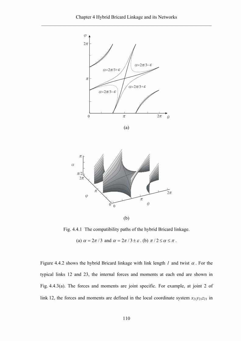
Chapter 4 Hybrid Bricard Linkage and its Networks
———————————————————————————————————
110
0
/3+2=
/3−2=
/3−2=
/3+2=
2
2
(a)
00
2
2/2
(b)
Fig. 4.4.1 The compatibility paths of the hybrid Bricard linkage.
(a) 3/2πα = and επα ±= 3/2 . (b) παπ ≤≤2/ .
Figure 4.4.2 shows the hybrid Bricard linkage with link length l and twist α . For the
typical links 12 and 23, the internal forces and moments at each end are shown in
Fig. 4.4.3(a). The forces and moments are joint specific. For example, at joint 2 of
link 12, the forces and moments are defined in the local coordinate system x21y21z21 in

Chapter 4 Hybrid Bricard Linkage and its Networks
———————————————————————————————————
111
which z21 is alongside the link while y21 is along the axis of joint 2. At joint 1, z12 is
alongside the link while y12 is along the axis of joint 1. Similarly, we are able to define
forces and moments for link 23.
Because of symmetry, the local forces and moments in link 34 should be the same as
those in link 12.
1
2
3
4
5
6
Fig. 4.4.2 A typical hybrid Bricard linkage.
Considering the equilibrium of link 12, we have
0sincos 121221 =−+ αα NyNxNx
0cossin 121221 =++ αα NyNxNy
01221 =+ NzNz
0sincos 21121221 =⋅−−+ lNyMyMxMx αα
0cossin 21121221 =⋅+++ lNxMyMxMy αα
01221 =+ MzMz
(4.4.1)

Chapter 4 Hybrid Bricard Linkage and its Networks
———————————————————————————————————
112
Nx21
My21Nz21
Mx21
Ny21
Mz21
Nx12
Mz12
Mx12Ny12
Nz12My12
Nx21
Ny21
Nx12Ny12
Link 12
Joint 2
Joint 1
Nx23
My23Nz23
Mx23
Ny23
Mz23
Nx32
Mz32
Mx32
Ny32
Nz32My32
Nx23
Ny23
Nx32
Ny32
Link 23
Joint 2
Joint 3
(a)
Nx21
Nz21
Mx21
Mz21
Nx23 Nz23Mx23
Mz23
Link 12 Link 23
Joint 2
Axis of Joint 2
Ny21Ny23
My21
My23
Nx32
Mz32
Mx32Nz32
Nx12
Mz12
Mx12
Nz12
Link 34Link 23
Joint 3
Axis of Joint 3
Ny12Ny32
My12
My32
(b)
Fig. 4.4.3 Equilibrium of links and joints.
(a) Forces and moments in two typical links; (b) forces and moments at joints 2 and 3.

Chapter 4 Hybrid Bricard Linkage and its Networks
———————————————————————————————————
113
The equilibrium equations for link 23 are
0sincos 232332 =−+ αα NyNxNx
0cossin 232332 =++ αα NyNxNy
03223 =+ NzNz
0sincos 32232332 =⋅+−+ lNyMyMxMx αα
0cossin 32232332 =⋅−++ lNxMyMxMy αα
03223 =+ MzMz
(4.4.2)
Links 12 and 23 are connected at joint 2 where the axis of the joint is in the direction of
y21 and y23, see Fig. 4.4.3(b). The equilibrium equations at joint 2 are
0sinsincoscos 23212321 =+−−− µµµµ NzNzNxNx
02321 =−− NyNy
0coscossinsin 23212321 =−−− µµµµ NzNzNxNx
0sinsincoscos 23212321 =+−−− µµµµ MzMzMxMx
02321 =−− MyMy
0coscossinsin 23212321 =−−− µµµµ MzMzMxMx
(4.4.3)
where 2
ϕπµ −= , which is half of the angle between links 12 and 23.
Links 23 and 34 are connected at joint 3 whose axis is in the same direction as y12 and
y32, see Fig. 4.4.3(b), because the local forces in link 34 are the same as those in link 12.
The equilibrium equations at joint 3 are

Chapter 4 Hybrid Bricard Linkage and its Networks
———————————————————————————————————
114
0sinsincoscos 32123212 =+−−− νννν NzNzNxNx
03212 =−− NyNy
0coscossinsin 32123212 =−−− νννν NzNzNxNx
0sinsincoscos 32123212 =+−−− νννν MzMzMxMx
03212 =−− MyMy
0coscossinsin 32123212 =−−− νννν MzMzMxMx
(4.4.4)
where 2
θπν −= , which is half of the angle between links 23 and 34.
Because the revolute joint cannot transform the moment in its axis direction,
0
0
3212
2321
==
==
MyMy
MyMy (4.4.5)
Substituting (4.4.5) into (4.4.1)-(4.4.4) gives
µtan2321 ⋅= NzNx , α
αµνsin
costantan2321
−⋅= NzNy , 2321 NzNz −=
lNzMx ⋅⋅=αν
sintan
2321 , 021 =My , lNzMz ⋅⋅=α
νµsin
tantan2321
νtan2312 ⋅−= NzNx , α
ανµsin
costantan2312
−⋅= NzNy , 2312 NzNz =
232323232323
2312122312
,sin
costantan,tan
sintantan,0,
sintan
NzNzNzNyNzNx
lNzMzMylNzMx
=+−
=⋅=
⋅⋅−==⋅⋅−=
ααµνµ
ανµ
αµ
(4.4.6)
lNzMx ⋅⋅−=αν
sintan
2323 , 023 =My , lNzMz ⋅⋅=α
νµsin
tantan2323

Chapter 4 Hybrid Bricard Linkage and its Networks
———————————————————————————————————
115
νtan2332 ⋅−= NzNx , α
ανµsin
costantan2332
+−⋅= NzNy , 2332 NzNz −=
lNzMx ⋅⋅=αµ
sintan
2332 , 032 =My , lNzMz ⋅⋅−=α
νµsin
tantan2332
In general, (4.4.6) presents one state of self-stress because if one variable, i.e., 23Nz , is
given, all the rest can be determined. However, when 3/2πα = , this changes at point
),( ππ , i.e. 0== νµ . Considering (4.4.5), the solution of (4.4.1)-(4.4.4) becomes
2321 NzNz −= , 2312 NzNz =
2323 NzNz = , 2332 NzNz −=
2321 MzMz −= , 2312 MzMz = (4.4.7)
2323 MzMz = , 2332 MzMz −=
The rest of forces and moments are zero.
Now, there are two independent variables, e.g., 23Nz and 23Mz . Thus, two states of self-
stress exist. Therefore, point ) ,( ππ is a point of kinematic bifurcation.
So far, we have proven that the kinematic indeterminacy of the linkage increases by one
at πϕθ == . The physical model shows that at πϕθ == , the degree of infinitesimal
mobility indeed increases by 1 because in this configuration, the axes of the three joints
at the top are coplanar and intersect at a single point, and so are the axes of the other
three joints at the bottom, see Fig. 4.2.5(a). This leads to two degrees of infinitesimal
mobility (Phillips, 1990). Although a bifurcation exists, it does not cause any problem in
deployment of the linkage because the links would have to penetrate each other in order

Chapter 4 Hybrid Bricard Linkage and its Networks
———————————————————————————————————
116
to reach the bifurcated position, which is physically impossible. The movement of the
linkage at πϕθ == effectively changes from one path to another toward a direction
such that the values of θ and ϕ decrease, instead of increasing. In such a situation, one
of two of the infinitesimal mobilities becomes finite while the other disappears.
4.5 ALTERNATIVE FORMS OF HYBRID BRICARD LINKAGE
Although the original hybrid Bricard linkage has already produced a compact folded
configuration, it is hard to realize in practice. The angle between six pairs of connected
bars cannot become zero simultaneously without a complex design. Hence, it is
important to investigate alternative forms of the hybrid Bricard linkages.
The method applied to find the alternative form of hybrid Bricard linkage is the same as
that in Section 3.3. The axes of revolute joints are extended and joints are connected
with bars not perpendicular to the axes, see Fig. 4.5.1, where the dashed lines present
the links of the original linkage and the solid lines present the bars in the alternative
form.
A0
A
B0
B
C0
C
D0
D
F0
F
E0
E
Fig. 4.5.1 The alternative form of hybrid Bricard linkage.

Chapter 4 Hybrid Bricard Linkage and its Networks
———————————————————————————————————
117
For simplicity, let us assume that symmetry is kept in the alternative form. Denote the
link length and twist of the original hybrid Bricard linkage in Fig. 4.5.1 as l and α ,
respectively. We have
d
c
===
===
FFDDBB
EECCAA
000
000
(4.5.1)
So all the bars of the alternative form have the same length, L , which is
αcos2FAEFDECDBCAB 222 cddclL −++======= (4.5.2)
For each given set of c and d , an alternative form for the hybrid Bricard linkage can be
obtained. The most compact folding can be achieved if simultaneously the points A, C
and E meet at a point while the points B, D and F also meet at another point. This means
that physically the linkage becomes a bundle whose length is L . Denote θ and ϕ in
this fully folded configuration as fθ and fϕ , respectively. On the other hand, when the
linkage is full expanded, points A, B, C, D, E, and F are on the same plane, i.e. the
linkage is completely flattened to form an equilateral hexagon. Take θ and ϕ in this
configuration as dθ and dϕ .
The relationship among the geometric parameters of the hybrid Bricard linkage and the
design parameters of the linkage in the alternative forms can be found geometrically as
we did in Section 3.3.2. Several alternative forms have been studied. Here only the most
interesting ones are listed.

Chapter 4 Hybrid Bricard Linkage and its Networks
———————————————————————————————————
118
For the linkage found by Gan and Pellegrino (2003) shown in Fig. 4.5.2, the geometric
parameters of its original hybrid Bricard linkage and its alternative form are
137arccos−= πα
2019arccos+= πθ f ,
2019arccos−= πϕ f
207arccos2 += πθ d ,
207arccos2 −= πϕd (4.5.3)
lL ⋅= 10103
ldc ⋅==60130
Fig. 4.5.2 A hybrid Bricard linkage in its alternative from.
(Courtesy of Professor Pellegrino of Cambridge University).

Chapter 4 Hybrid Bricard Linkage and its Networks
———————————————————————————————————
119
It is particularly interesting to mention two linkages, both of which are based on the
same alternative form of the same hybrid Bricard linkage. During the folding process,
one is blocked while the other is not.
The first linkage was proposed by Pellegrino (2002). For convenience, let us call it
Linkage I. A reproduction of Linkage I is given in Fig. 4.5.3. The other, namely
Linkage II, is shown in Fig. 4.5.4. The geometric parameters of the original hybrid
Bricard linkage and its alternative form of both linkages are as follows.
2arctan−= πα
πθ32
−=f , 715arctan−=fϕ
πθ32
=d , 0=dϕ (4.5.4)
lL ⋅= 332
lc ⋅=63 , ld ⋅=
615
The compatibility path of both linkages is shown in Fig. 4.5.5. When the models are
fully expanded, they are flat, corresponding to point D in the compatibility path. The
completely folded position corresponds to point F in the path.
The similarity of these two linkages ends here.

Chapter 4 Hybrid Bricard Linkage and its Networks
———————————————————————————————————
120
(a) (b)
Fig. 4.5.3 Deployment of Linkage I.
(a) Fully expanded configuration; (b) blockage occurs during folding.
(a) (b)
(c) (d)
Fig. 4.5.4 Deployment of Linkage II.
(a) Fully expanded; (b) – (c) intermediate; (d) fully folded configurations.

Chapter 4 Hybrid Bricard Linkage and its Networks
———————————————————————————————————
121
For Linkage I, the folding process can be traced along the compatibility path from D to
F via B, see Fig. 4.5.5. However, the movement of linkage is found to be physically
blocked at point B because the ends of bars of hit each other, see Fig. 4.5.3(b). This
model is made from solid steel bars and brass hinges, which are fairly rigid and allow
almost no deformation. Hence, the deployment terminates at B.
Pellegrino (2002) also observed that the linkage did fold up if it is made from less rigid
material such as card or weak hinges. While folding, a force has to be applied to linkage
to enable joints deform slightly. A model shown in Fig. 4.5.6, which is made from card,
demonstrates this process. After moving from the configuration shown in Fig. 4.5.6(a)
to that in Fig. 4.5.6(b) during folding, a force is applied to make the model folded to that
in Fig. 4.5.6(c) and then to that in Fig. 4.5.6(d).
0 D
B
F
F’
AC
E
2
2
−
−
Fig. 4.5.5 The compatibility path of the 6R linkage with twist 2arctan−= πα .

Chapter 4 Hybrid Bricard Linkage and its Networks
———————————————————————————————————
122
(a) (b)
(c) (d)
Fig. 4.5.6 Card model of Linkage I.
(a) At D, (b) B, (c) E and (d) F′ of the compatibility path.
A close examination of the compatibility path reveals that, in the card model, the
folding process corresponds to a movement from D to F′, instead of F, due to the fact
that compatibility path is periodic and FF θπθ += 2' , FF ϕπϕ += 2' . The reason why
this happens is because 2arctan−= πα , i.e. 116.57°, is sufficient close to 3/2π , i.e.
120°. As we discussed in the previous section, πϕθ == is a point of bifurcation for
the 6R linkage with twist 3/2π . Hence, when the force is applied to the linkage with
2arctan−= πα , an imperfection is introduced to the twist of the linkage which alters to
3/2π . The folding process reaches bifurcation point E. When the force is released, the

Chapter 4 Hybrid Bricard Linkage and its Networks
———————————————————————————————————
123
twist of linkage changes back to 2arctan−= πα . Accordingly, (θ , ϕ ) reaches point
F′.
Linkage II behaves differently. The folding process takes route from D to F via A and
C. There is no blockage during deployment and the structure can be folded up
completely, as shown in Fig. 4.5.4.
4.6 CONCLUSION AND DISCUSSION
This chapter has presented a method to construct a large structural mechanism using the
hybrid Bricard linkages as basic elements. It has the same features as the structural
mechanism based on the Bennett linkage, e.g., it has a single degree of mobility,
consists of simple revolute joints and possesses overconstrained geometry.
The chapter started with a derivation of the hybrid Bricard linkage from the general
plane-symmetric and trihedral Bricard linkages. This hybrid linkage is overconstrained
with a single degree of mobility. Its compatibility condition was presented.
The second part of this chapter was devoted to the study of the deployment
characteristics of the hybrid Bricard linkage. We found all hybrid Bricard linkages can
expand to a planar equilateral triangle, and in particular, when the twists are 3/π or
3/2π , the hybrid Bricard linkages can be folded completely. This feature allows the
construction of networks of hybrid Bricard linkages.

Chapter 4 Hybrid Bricard Linkage and its Networks
———————————————————————————————————
124
As a result, we proposed a scheme to build large deployable networks using the hybrid
Bricard linkages. It has been proven to be successful.
It has also been noticed that branches exist at certain points along the compatibility
paths. We have proved the existence of bifurcation points by identifying a change in the
number of states of self-stresses in the linkage. We have also demonstrated that the
bifurcation itself does not cause any problem in deployment.
Finally, alternative forms of hybrid Bricard linkage have been discussed with examples.
Their deployed configuration is a hexagon and their folded configuration is a bundle.
We have shown that the identical alternative form could lead to complete deployment
behaviour: one with deployment blockage while the other without. Although the current
method is not able to model deployment blockage of the structure, we have shown how
a blocked configuration can be re-configured to achieve full deployment.
The work presented has shown that the approach is valid. It also points us to the fact
that more work should be done to set up the relationship between the original hybrid
Bricard linkage and its alternative forms, and to find a way to model deployment
blockage. Networks of the hybrid Bricard linkage in the alternative forms could be
developed as we did for the Bennett linkage.

125
5
Tilings for Construction of Structural
Mechanisms
5.1 INTRODUCTION
In the previous two chapters, we presented the construction of networks of Bennett
linkages and hybrid Bricard linkages. We did not, however, give any reason why a
particular network pattern was chosen. Neither did we show the existence of other
network patterns. In this chapter, we will explain how we arrived at those particular
network patterns.
In general, a network could consist of an unlimited number of basic linkages. For
practical reasons, it is sensible to consider that the number of the types of basic linkages
is small and these linkages are regularly repeated in the network. Due to this
simplification, the mathematic tiling technique can be adopted to find the possible
arrangements of networks.
As reviewed in Section 2.3, the total number of distinct k-uniform tilings is 135. These
tilings can be modified into many more tilings and patterns with methods such as

Chapter 5 Tilings for Construction of Structural Mechanisms
———————————————————————————————————
126
transformation of symmetry, transitivity and regularity, tilings that are not edge-to-edge,
and patterns with overlap motifs, etc. In spite of their large number, all of the tilings can
be considered as a tessellation unit in one of these three (36), (44) and (63) tilings
involving a single type of regular polygon. If, in the construction of structural
mechanisms, we take the basic linkage or assembly of a set of linkages as a basic
tessellation unit, the tiling technique can then be used to guide us towards suitable
arrangements in which units are connected repeatedly following the three tilings
mentioned above. Hence, the key questions are, first of all, how a tessellation unit in the
form of a triangle, square or hexagon can be built and secondly whether the
compatibility requirements can be met in a particular assembly.
The layout of the chapter is as follows. Sections 5.2 and 5.3 present tiling and its
application to the networks of Bennett linkages and hybrid Bricard linkages,
respectively. Some conclusions and discussion follow in Section 5.4.
5.2 NETWORKS OF BENNETT LINKAGES
The Bennett linkage consists of four bars and therefore tilings of squares can be used as
possible arrangements of a network of Bennett linkages.
5.2.1 Case A
Figure 5.2.1(a) is a schematic diagram of a Bennett linkage, in which four links are

Chapter 5 Tilings for Construction of Structural Mechanisms
———————————————————————————————————
127
connected at A, B, C and D. (44) tiling presents the simplest way to form a network in
which another similar Bennett linkage is connected on the right of CD, see Fig. 5.2.1(b).
The process can be repeated for other sides.
Now let us examine the two Bennett linkages shown in Fig. 5.2.1(b). The structure has
more than one degree of mobility because Bennett linkages ABCD and DCFE can move
independently. Goldberg (1943) suggested that links BC and CF could be welded
together, resulting in a Goldberg 5R linkage. However, the same process cannot be
repeated for other adjacent Bennett linkages unlimitedly. Hence, this arrangement does
not work.
A D
CB
A D
CB
E
F
(a) (b)
Fig. 5.2.1 (a) A Bennett linkage; (b) two Bennett linkages connected.
5.2.2 Case B
Let us now modify the unit to that shown in Fig. 5.2.2(a), in which the links are
extended while the revolute joints remain at A, B, C and D. A network can then be
formed, see Fig. 5.2.2(b). Next, we will examine whether such an arrangement will
produce a structural mechanism.

Chapter 5 Tilings for Construction of Structural Mechanisms
———————————————————————————————————
128
Take
aaa == CDAB , baa == DABC
ααα == CDAB , βαα == DABC
akaaaa S==== DKBICGAE , bkaaaa S==== DHBFCJAL
ααααα ==== DKBICGAE , βαααα ==== DHBFCJAL
(5.2.1)
where 10 << Sk .
Hence, all of the Bennett linkages in Fig. 5.2.2(b) satisfy the geometric condition for
Bennett linkages.
A D
CB
H
E
F
G
L1
L2
L4
L3
A D
CB
H
E
F
G
I
L
J
K
(a) (b)
Fig. 5.2.2 (a) A unit based on the Bennett linkage; (b) network of units.

Chapter 5 Tilings for Construction of Structural Mechanisms
———————————————————————————————————
129
Considering Bennett linkages L1, L2, L3 and L4, we have
( )
( )αβ
αβφσ
−
+=
21sin
21sin
2tan
2tan (5.2.2a)
( )
( )αβ
αβτπσπ
−
+=
−−
21sin
21sin
2tan
2tan (5.2.2b)
( )
( )αβ
αβυτ
−
+=
21sin
21sin
2tan
2tan (5.2.2c)
( )
( )αβ
αβυπφπ
−
+=
−−
21sin
21sin
2tan
2tan (5.2.2d)
Combining (5.2.2a) and (5.2.2c), as well as (5.2.2b) and (5.2.2d) gives
( )
( )
( )
( )
2
2
21sin
21sin
2tan
2tan
2tan
2tan
21sin
21sin
2tan
2tan
2tan
2tan
+
−=
−
+=
αβ
αβυτσφ
αβ
αβυτσφ
(5.2.3)
From (5.2.3), we obtain that
( )
( )1
21sin
21sin
±=+
−
αβ
αβ(5.2.4)

Chapter 5 Tilings for Construction of Structural Mechanisms
———————————————————————————————————
130
There are four possibilities for any πβα 2,0 ≤≤ .
αβαβ +=−
)( αβαβ +−=−
παβαβ 2)( +−=+
παβαβ 2)( +−−=+
(5.2.5)
leading to
0=α , or πα = , and 0=β , or πβ = (5.2.6)
It can be concluded from (5.2.6) that only when α and β are 0 or π , can a mobile
network based on the tiling shown in Fig. 5.2.2(b) be constructed. In each solution, the
Bennett linkage is a 2D four-bar chain. For Bennett linkages with any other twists, it is
impossible to construct a mobile network with the arrangement as shown in
Fig. 5.2.2(b).
5.2.3 Case C
Now let us modify the unit further to that shown in Fig. 5.2.3, in which all of the links
are extended at both ends.
Applying this unit to the (44) tiling produces the network shown in Fig. 3.2.4. From the
discussion in Section 3.2, we know that the network is mobile with a single degree of
mobility.

Chapter 5 Tilings for Construction of Structural Mechanisms
———————————————————————————————————
131
A
D
C
BH
EF
G
I
L
J
K
Fig. 5.2.3 A unit based on the Bennett linkage.
5.3 NETWORKS OF HYBRID BRICARD LINKAGES
5.3.1 Case A
The hybrid Bricard linkage has six equal links. Naturally, we think of (63) tiling to form
a network.
Consider a portion of the network shown in Fig. 5.3.1. Loops L1, L2, and L3 are all made
of identical hybrid Bricard linkages with twists α and απ −2 , alternating from one
link to the other. Take
αα =AC (5.3.1)
Then for loop L2,
απα −= 2BA (5.3.2)
Considering loop L3 gives
απα −= 2AD (5.3.3)

Chapter 5 Tilings for Construction of Structural Mechanisms
———————————————————————————————————
132
A
C
B DL1
L3L2
Fig. 5.3.1 A network of hybrid Bricard linkage.
Now a problem arises, as for loop L1,
απαα −== 2ADBA (5.3.4)
which means that loop L1 violates the condition of the hybrid Bricard linkage. Thus, the
network consisting of more than one such deployable element will become immobile.
5.3.2 Case B
In Section 4.2, we showed that the hybrid Bricard linkage deploys a triangular shape
shown in Fig. 5.3.2(a). Thus, it may be possible to use (36) tiling to construct a network.
A typical connection of hybrid Bricard linkages in the (36) tiling is as shown in
Fig. 5.3.2(b), in which the central linkage shares two common links with each of the
adjacent linkages. The projection of its probable deployment sequence is shown in
Figs. 5.3.2(c) and 5.3.2(d). It becomes obvious that the central linkage behaves
completely differently from those around it. Hence, such an arrangement cannot be used
to construct a mobile network.

Chapter 5 Tilings for Construction of Structural Mechanisms
———————————————————————————————————
133
A
B C
(a) (b)
A
B C
AB
C
(c) (d)
Fig. 5.3.2 (a) A hybrid Bricard linkage with twists of 3/π or 3/2π ;
(b) possible connections; (c) and (d) projection of probable deployment sequence.
5.3.3 Case C
The unit can be modified further to that shown in Fig. 5.3.3. The unit can be tessellated
by (36) tiling to make a network, which has been the subject of discussion in
Section 4.3. The projection of the network during deployment is given in Fig. 5.3.4. It is
shown that every hybrid Bricard linkage behaves in the same fashion all the time during
the deployment process, which guarantees the compatibility of the network.

Chapter 5 Tilings for Construction of Structural Mechanisms
———————————————————————————————————
134
Fig. 5.3.3 A unit based on the hybrid Bricard linkage.
Fig. 5.3.4 Projection of a network of hybrid Bricard linkages during deployment.
Chapter 5 Tilings for Construction of Structural Mechanisms
———————————————————————————————————
135
5.4 CONCLUSION AND DISCUSSION
This chapter has presented a method to build structural mechanisms using deployable
unit and tilings and patterns. It involves three steps: selection of suitable tilings,
construction of units using overconstrained linkage and validation of compatibility.
This method has been applied to the networks consisting of Bennett linkages and hybrid
Bricard linkages, respectively. (36), (44) and (63) tilings have been adopted and several
units have been discussed. The structural mechanisms based on Bennett linkages and
hybrid Bricard linkages that described in previous two chapters were reconstructed by
this tessellation method.
It should be pointed out that there are many ways of constructing deployable units
including the units made from a combination of more than one type of 3D
overconstrained linkages. Many examples concerning tilings and patterns can be found
from references such as Grünbaum and Shephard (1986). We have not attempted all the
possibilities. Instead a few simple examples have been used to illustrate that the
approach is valid.

136
6
Final Remarks
The aim of this dissertation was to explore ways of constructing structural mechanisms
using the existing 3D overconstrained linkages consisting of only hinged joints. In this
chapter, we summarise the main achievements in the design of 3D structural
mechanisms and highlight future work needed.
6.1 MAIN ACHIEVEMENTS
• Structural mechanisms based on Bennett linkages
The first effort of this dissertation was to construct large overconstrained structural
mechanisms using Bennett linkages as basic elements.
We have found the basic layout of a structure allowing unlimited extension of the
network. We were able to produce a family of networks of Bennett linkages to form
single-layer structural mechanisms, which, in general, deploy into profiles of cylindrical
surface. Meanwhile, we have discussed two special cases of the single-layer structures
that can be extended to multi-layer structural mechanisms. In addition, according to our

Chapter 6 Final Remarks
———————————————————————————————————
137
derivation, we have found a solution to a problem which other researchers have been
unable to solve, i.e., how to connect two similar Bennett linkages to form a mobile
structure.
A mathematical proof of the existence of alternative forms of Bennett linkages has also
been presented, which enables the linkage to be folded completely. Under certain
circumstances, the said forms also allow the linkage to be flattened completely, giving
maximum expansion. This work has resulted in the creation of the most effective
deployable element based on Bennett linkage. A simple method to build the Bennett
linkage in its alternative form has been introduced and verified. The corresponding
networks have been obtained following the similar layouts of the original Bennett
linkage.
All of the structural mechanisms contain only revolute joints, have a single degree of
mobility and are geometrically overconstrained.
• Structural mechanisms based on hybrid Bricard linkages
A similar method has been developed to construct large overconstrained structural
mechanisms using hybrid Bricard linkages as basic elements.
The hybrid Bricard linkage is a special case of the Bricard linkage. This linkage is
overconstrained and with a single degree of mobility. We have derived its compatibility
condition and studied its deployment behaviour. It has been found that for some

Chapter 6 Final Remarks
———————————————————————————————————
138
particular twists, the hybrid Bricard linkage can be folded completely into a bundle and
deployed to a flat triangular profile. Based on this linkage, we have constructed a
network of the hybrid Bricard linkages. Furthermore, we have studied the deployment
characteristics including kinematic bifurcation and the alternative forms of the hybrid
Bricard linkage.
The proposed structural mechanisms exhibit the same features as those based on the
Bennett linkage.
• Tilings
We have applied the tilings and patterns to the construction of the networks based on
the Bennett linkages and hybrid Bricard linkages. Several possible configurations have
been discussed including those described previously.
A general approach to construct large structural mechanisms has been proposed, which
can be divided into three steps: selection of suitable tilings, construction of
overconstrained units and validation of compatibility.
6.2 FUTURE WORKS
The research reported in this dissertation opens up many opportunities for further study.

Chapter 6 Final Remarks
———————————————————————————————————
139
First of all, for assemblies of Bennett linkages our solution is largely based on the
compatibility equations. There may be other solutions. Further study of the highly non-
linear compatibility conditions is needed to either find or rule out other solutions.
Secondly, the work dealing with alternative forms of the hybrid Bricard linkage shows
that the approach is valid. More work should be done to set up the general relationship
between the original hybrid Bricard linkage and its alternative form. Networks of the
hybrid Bricard linkage in the alternative forms could also be developed as we did for the
Bennett linkage.
Thirdly, during the construction of networks of linkages, we have considered only one
type of linkage at a time. With the application of tiling, units consisting of more than
one type of linkage can be considered. For example, the deployable element based on
the Bennett linkage and that based on the hybrid Bricard linkage maybe can be
combined together following (33.42) tiling.
Fourthly, the approach presented in this dissertation has only been applied to the
Bennett and Bricard linkages. It can be extended to all the existing 3D overconstrained
linkages, e.g. Myard linkage, Altmann linkage, Sarrus linkage, Waldron hybrid linkage,
and Wohlhart linkage. More structural mechanisms could be found in this way.
Furthermore, in the mathematical derivation, the cross-sectional dimension of links has
been ignored, so the current modelling is not capable of predicting conflict in the
deployment process. Discussion on blockage of deployment has been mainly based on

Chapter 6 Final Remarks
———————————————————————————————————
140
experiments. Hence, a detailed modelling process, which is closer to the physical
models, will be highly desirable.
Finally, although the approach presented in this dissertation has led to discovery of
many new structures, it does not consider the deployed configuration in the design
process. Instead, it is checked after a structural mechanism is obtained. In engineering
practice, deployed configuration is the most important design consideration. How to
integrate this consideration into the current approach will be a natural step forward to
make this work more attractive to practical engineers.

141
References
Altmann, P G (1954), Communications to Grodzinski, P. and M’Ewen, E, Link
mechanisms in modern kinematics, Proceedings of the Institution of Mechanical
Engineers, 168(37), 889-896.
Baker, E J (1975), The Delassus linkages, Proceedings of Fourth World Congress on
the Theory of Machines and Mechanisms, Newcastle upon Tyne, England, Sept 8-13,
paper No. 9, 45-49.
Baker, E J (1978), Overconstrained 5-bars with parallel adjacent joint axes I & II,
Mechanism and Machine Theory, 13, 213-233.
Baker, E J (1979), The Bennett, Goldberg and Myard linkages – in perspective,
Mechanism and Machine Theory, 14, 239-253.
Baker, E J (1980), An analysis of Bricard linkages, Mechanism and machine Theory 15,
267-286.
Baker, E J (1984), On 5-revolute linkages with parallel adjacent joint axes, Mechanism
and Machine Theory, 19(6), 467-475.
Baker, E J (1986), Limiting positions of a Bricard linkage and their possible relevance
to the cyclohexane molecule, Mechanism and Machine Theory, 21(3), 253-260.
Baker, E J (1988), The Bennett linkage and its associated quadric surfaces, Mechanism
and Machine Theory, 23(2), 147-156.
Baker, E J (1993), A geometrico-algebraic exploration of Altmann’s linkage,
Mechanism and Machine Theory, 28(2), 249-260.
Baker, E J (1998), On the motion geometry of the Bennett linkage, Proceeding 2 of
Eighth International Conference on Engineering Computer Graphic and Descriptive
Geometry, Austin, USA, 31 July-3 August, 433-437.

References
———————————————————————————————————
142
Baker, E J (2001), The axodes of the Bennett linkage, Mechanism and Machine Theory,
36, 105-116.
Baker, E J (2002), Displacement-closure equations of the unspecialised double-
Hooke’s-joint linkage, Mechanism and Machine Theory, 37, 1127-1144.
Baker, E J, Duclong, T and Khoo, P S H (1982), On attempting to reduce undesirable
inertial characteristics of the Schatz mechanism, Trans. ASME, Journal of Mechanical
Design, 104, 192-205.
Baker, E J and Hu, M (1986), On spatial networks of overconstrained linkages,
Mechanism and Machine Theory, 21(5), 427-437.
Beggs, J S (1966), Advanced Mechanism, Macmillan Company, New York.
Bennett, G T (1903), A new mechanism, Engineering, 76, 777-778.
Bennett, G T (1905), The parallel motion of Sarrus and some allied mechanisms,
Philosophy Magazine, 6th series, 9, 803-810.
Bennett, G T (1911), Deformable octahedra, Proceeding of London Mathematics
Society, 2nd series, 10(1), 309-343.
Bennett, G T (1914), The skew isogram mechanism, Proceeding of London
Mathematics Society, 2nd series, 13, 151-173.
Beverley, D (1999), Tiling and Mosaics in a Weekend, Merehurst, London.
Brát, V (1969), A six-link spatial mechanism, Journal of Mechanisms, 4, 325-336.
Bricard, R (1927), Leçons de cinématique, Tome II Cinématique Appliquée, Gauthier-
Villars, Paris, 7-12.
Calladine, C R (1978), Buckminster Fuller’s “tensegrity” structures and Clerk
Maxwell’s rules for the construction of stiff frames, Int. J. Solids Structures, 14, 161-
172.
Calladine, C R and Pellegrino S (1991), First-order infinitesimal mechanisms, Int. J.
Solids Structures, 27(4), 505-515.
References
———————————————————————————————————
143
Crawford, R F, Hedgepeth, J M and Preiswerk, P R (1973), Spoked wheels to deploy
large surfaces in space: weight estimates for solar arrays, NASA-CR-2347.
Critchlow, K (1969), Order in Space, a design source book, Thams and Hudson,
London.
Cundy, H M and Rollett, A P (1961), Mathematical Models, Tarquin Publications,
Oxford.
Delassus, E (1922), Les chaînes articulées fermées et déformables à quatre membres,
Bulletin des Sciences Mathématiques, 2nd series, 46, 283-304.
Dietmaier, P (1995), A new 6R space mechanism, Proceeding 9th World Congress
IFToMM, Milano, 1, 52-56.
Evans, J (1931), Pattern : a study of ornament in western Europe from 1180 to 1900,
Clarendon Press, Oxford.
Gan, W W and Pellegrino, S (2003), Closed-loop deployable structures, AIAA 2003-
1450, Proceeding of 44th AIAA/ASME/ASCE/AHS/ASC Structures, Structural
Dynamics, and Materials Conference, 7-10 April 2003, Norfolk, VA.
Goldberg, M (1943), New five-bar and six-bar linkages in three dimensions, Trans.
ASME, 65, 649-663.
Grünbaum, B and Shephard, G C (1986), Tilings and Patterns, W. H. Freeman and
Company, New York.
Ho, C Y (1978), Note on the existence of Bennett mechanism, Mechanism and Machine
Theory, 13(3), 269-271.
Huang, C (1997), The cylindroid associated with finite motions of the Bennett
Mechanism, Trans. ASME, Journal of Engineering for Industry, 119, 521-524.
Hunt, K H (1978), Kinematic Geometry of Mechanisms, Oxford University Press,
Oxford.
Magnus, W (1974), Noneuclidean tesselations and their groups, Academic Press, New
York.

References
———————————————————————————————————
144
Mavroidis, C and Roth, B (1994), Analysis and synthesis of overconstrained
mechanism, Proceeding of the 1994 ASME Design Technical Conference, Minneapolis,
MI, September, 115-133.
Myard, F E (1931), Contribution à la géométrie des systèmes articulés, Societe
mathématiques de France, 59, 183-210.
Pamidi, P R, Soni, A H and Dukkipati, R V (1973), Necessary and sufficient existence
criteria of overconstrained five-link spatial mechanisms with helical, cylinder, revolute
and prism pairs, Trans ASME, Journal of Engineering for Industry, 95, 737-743.
Pellegrino, S (2002), Personal communication.
Pellegrino S, Green C, Guest S D and Watt A (2000), SAR advanced deployable
structure, Technical Report, Department of Engineering, University of Cambridge.
Phillips, J (1984), Freedom of Machinery, Volume I, Cambridge University Press,
Cambridge.
Phillips, J (1990), Freedom of Machinery, Volume II, Cambridge University Press,
Cambridge.
Rogers, C A, Stutzman, W L, Campbell, T G and Hedgepeth, J M (1993), Technology
assessment and development of large deployable antennas, Journal of Aerospace
Engineering, 6(1), 34-54.
Rossi, F (1970), Mosaics : a survey of their history and techniques, Pall Mall Press,
London.
Sarrus, P T (1853), Note sur la transformation des mouvements rectilignes alternatifs,
en mouvements circulaires, et reciproquement, Académie des Sciences, 36, 1036-1038.
Savage, M (1972), Four-link mechanisms with cylindric, revolute and prismatic pairs,
Mechanism and Machine Theory, 7, 191-210.
Schattschneider, D and Walker, W (1977), M. C. Escher Kaleidocycles, Tarquin
Publications, England.
Steinhaus, H (1983), Mathematical Snapshots, Oxford University Press, Oxford.

References
———————————————————————————————————
145
Waldron, K J (1967), A family of overconstrained linkages, Journal of Mechanisms, 2,
210-211.
Waldron, K J (1968), Hybrid overconstrained linkages, Journal of Mechanisms, 3, 73-
78.
Waldron, K J (1969), Symmetric overconstrained linkages, Trans. ASME, Journal of
Engineering for Industry, B91, 158-164.
Wohlhart, K (1987), A new 6R space mechanism, Proceedings of the 7th World
Congress on the Theory of Machines and Mechanisms, Seville, Spain, 17-22 September,
1, 193-198.
Wohlhart, K (1991), Merging two general Goldberg 5R linkages to obtain a new 6R
space mechanism, Mechanism and Machine Theory, 26(2), 659-668.
Wohlhart, K (1993), The two type of the orthogonal Bricard linkage, Mechanism and
Machine Theory, 28(6), 807-817.
You, Z and Pellegrino, S (1993), Foldable ring structures, Space Structures 4, Vol. 1,
Ed. Parke G. A. R. and Howard, C. M. Thomas Telford, London, 1993, 783-792.
You, Z and Pellegrino, S (1997), Foldable bar structures, Int. J. solids Structures,
34(15), 1825-1847.
Yu, H-C (1981a), The Bennett linkage, its associated tetrahedron and the hyperboloid of
its axes, Mechanism and Machine Theory, 16, 105-114.
Yu, H-C (1981b), The deformable hexahedron of Bricard, Mechanism and Machine
Theory, 16(6), 621-629.
Yu, H-C (1987), Geometry of the Bennett linkage via its circumscribed sphere,
Proceeding of the 7th World Congress on the Theory of Machines and Mechanisms,
Seville, Spain, 17-22 September, 1, 227-229.