Design of an ad hoc wireless network for wildlife telemetry
110
Transcript of Design of an ad hoc wireless network for wildlife telemetry

Design of an ad hoc wireless network for wildlife
telemetry tracking in the Cederberg
by
Johan George Brits
Thesis presented in partial fullment of the requirements for
the degree of Master of Science in Electronic Engineering at
Stellenbosch University
Department of Electrical and Electronic Engineering,University of Stellenbosch,
Matieland, 7601, South Africa.
Supervisor: Dr. H.A. Engelbrecht
March 2011

Declaration
By submitting this thesis electronically, I declare that the entirety of the work containedtherein is my own, original work, that I am the owner of the copyright thereof (unless tothe extent explicitly otherwise stated) and that I have not previously in its entirety or inpart submitted it for obtaining any qualication.
Signature: . . . . . . . . . . . . . . . . . . . . . . . . . . . . . . . . .J.G Brits
2011/03Date: . . . . . . . . . . . . . . . . . . . . . . . . . . . . . . . . . . . .
Copyright© 2011 Stellenbosch UniversityAll rights reserved.
i

Abstract
Design of an ad hoc wireless network for wildlife telemetry
tracking in the Cederberg
J.G Brits
Department of Electrical and Electronic Engineering,
University of Stellenbosch,
Matieland, 7601, South Africa.
Thesis: MScEng (Electronic)
March 2011
This thesis involves research on wildlife telemetry tracking for the Cape Leopard Trust(CLT). The CLT needed a network to transfer GPS data and single frame photos fromremote locations in the Cederberg to a researcher's base station. The proposed solutionis an ad hoc wireless network, where nodes perform polling of leopard collars and sendinformation via the multi-hop network to the researcher's base once it is downloaded froma collar. The literature study involved medium access control - and routing protocols foreectively transferring information. The solution was implemented in hardware and rangetests were done in the Cederberg to determine feasible locations for nodes in this networkfor covering most of the CLT study area. Link budgets for this area was determined withRadio Mobile to compare with actual ranges as measured. The simulation of protocolswas done in OMNET++ which could be compared with actual results from the physicalnetwork.
ii

Uittreksel
Ontwerp van 'n ad hoc draadlose netwerk vir opsporing van
luipaarde in die Cederberge
(Design of an ad hoc wireless network for wildlife telemetry tracking in the Cederberg)
J.G Brits
Departement Elektriese en Elektoniese Ingenieurswese,
Universiteit van Stellenbosch,
Matieland 7601, Suid Afrika.
Tesis: MScIng (Elektronies)
Maart 2011
Hierdie tesis handel oor navorsing wat gedoen is vir die Kaapse Luipaard Trust (CLT)vir die opsporing van luipaarde. Die CLT het 'n netwerk nodig gehad wat GPS data enenkel raam fotos van afgeleë gebiede in die Cederberge na 'n navorser se basis stuur. Dievoorgestelde oplossing is 'n ad hoc draadlose netwerk, waar nodisse luipaard nekbandeoproep om data af te laai en dan te stuur deur die multi-hop netwerk na die navorserse basis. Die literatuurstudie handel oor medium toegangs beheer - en roete verkrygingprotokolle vir die eektiewe oordrag van informasie. Die oplossing is in hardeware geïm-plimenteer en radio-afstand-toetse is gedoen in die Cederberge om goedgeleë posisies virnodisse te bepaal om die grootste gedeelte van die CLT studie area te dek. Radio Mobileis gebruik om voorspellings te maak rakende die afstande verkrygbaar tussen radios omte vergelyk met die siese metings in die veld. Die simulasie van protokolle is gedoen inOMNET++ en vergelyk met prestasie metings op die siese netwerk.
iii

Acknowledgements
I would like to express my sincere gratitude to the following people and organizations:
My supervisor Dr. H.A. Engelbrecht for his guidance
Mr. Quinton Martins of the Cape Leopard Trust for answering project relatedquestions
Mr. J. Arendse for soldering the ve test units
Mr. W. Croucamp for hardware related services
Mr. A. Barnard for radio frequency related knowledge
Mr. D. Kotze for help with Omnet++
Mr. R. Wiid for his help with the range tests in the Cederberg
Mr. D. Warnich for various project related insights
Jean Mearns, Managing Director of W.H. Circuits for sponsoring the printed circuitboards of the tests units
My family for their support
My Saviour Jesus
iv

Dedications
Hierdie tesis word opgedra aan my ouers wat my elke oomblik ondersteun het deur my
ingenieurswese studies
v

Contents
Declaration i
Abstract ii
Uittreksel iii
Acknowledgements iv
Dedications v
Contents vi
List of Figures viii
List of Tables x
Nomenclature xi
1 Introduction 11.1 Motivation for this study . . . . . . . . . . . . . . . . . . . . . . . . . . . . 11.2 Background . . . . . . . . . . . . . . . . . . . . . . . . . . . . . . . . . . . 11.3 Existing solutions to obtaining wildlife tracking data . . . . . . . . . . . . 11.4 Advantages and disadvantages of wildlife telemetry tracking arising from
literature . . . . . . . . . . . . . . . . . . . . . . . . . . . . . . . . . . . . . 31.5 Objectives of this study . . . . . . . . . . . . . . . . . . . . . . . . . . . . 31.6 Contributions . . . . . . . . . . . . . . . . . . . . . . . . . . . . . . . . . . 41.7 Overview . . . . . . . . . . . . . . . . . . . . . . . . . . . . . . . . . . . . . 4
2 Literature study 62.1 Introduction . . . . . . . . . . . . . . . . . . . . . . . . . . . . . . . . . . . 62.2 Physical layer . . . . . . . . . . . . . . . . . . . . . . . . . . . . . . . . . . 72.3 Medium Access Control (MAC) and routing Protocol selection . . . . . . . 92.4 Addressing . . . . . . . . . . . . . . . . . . . . . . . . . . . . . . . . . . . . 172.5 Summary . . . . . . . . . . . . . . . . . . . . . . . . . . . . . . . . . . . . 18
3 Theoretical work 193.1 Design constraints . . . . . . . . . . . . . . . . . . . . . . . . . . . . . . . 193.2 Link Budget . . . . . . . . . . . . . . . . . . . . . . . . . . . . . . . . . . . 213.3 Summary . . . . . . . . . . . . . . . . . . . . . . . . . . . . . . . . . . . . 30
4 Communication Strategy 31
vi

CONTENTS vii
4.1 Introduction . . . . . . . . . . . . . . . . . . . . . . . . . . . . . . . . . . . 314.2 Medium Access Control protocol description . . . . . . . . . . . . . . . . . 314.3 Routing protocol description . . . . . . . . . . . . . . . . . . . . . . . . . . 414.4 Summary . . . . . . . . . . . . . . . . . . . . . . . . . . . . . . . . . . . . 47
5 Hardware Design 485.1 Introduction . . . . . . . . . . . . . . . . . . . . . . . . . . . . . . . . . . . 485.2 System design . . . . . . . . . . . . . . . . . . . . . . . . . . . . . . . . . . 485.3 Component selection . . . . . . . . . . . . . . . . . . . . . . . . . . . . . . 505.4 Circuit design . . . . . . . . . . . . . . . . . . . . . . . . . . . . . . . . . . 605.5 Cost . . . . . . . . . . . . . . . . . . . . . . . . . . . . . . . . . . . . . . . 655.6 System verication . . . . . . . . . . . . . . . . . . . . . . . . . . . . . . . 655.7 Summary . . . . . . . . . . . . . . . . . . . . . . . . . . . . . . . . . . . . 67
6 Experimental investigation 746.1 Introduction . . . . . . . . . . . . . . . . . . . . . . . . . . . . . . . . . . . 746.2 Error performance of radio . . . . . . . . . . . . . . . . . . . . . . . . . . . 746.3 Throughput . . . . . . . . . . . . . . . . . . . . . . . . . . . . . . . . . . . 756.4 Route acquisition delay . . . . . . . . . . . . . . . . . . . . . . . . . . . . . 806.5 Range tests - eldwork . . . . . . . . . . . . . . . . . . . . . . . . . . . . . 816.6 Power performance . . . . . . . . . . . . . . . . . . . . . . . . . . . . . . . 866.7 Summary . . . . . . . . . . . . . . . . . . . . . . . . . . . . . . . . . . . . 86
7 Conclusions and recommendations 887.1 Summary and conclusions . . . . . . . . . . . . . . . . . . . . . . . . . . . 887.2 Comparison to prior work . . . . . . . . . . . . . . . . . . . . . . . . . . . 887.3 Outstanding issues . . . . . . . . . . . . . . . . . . . . . . . . . . . . . . . 897.4 Recommendations for future work . . . . . . . . . . . . . . . . . . . . . . . 89
Appendices 90
A PCB layout 91
B Project Pictures 94
Bibliography 95

List of Figures
2.1 OSI model . . . . . . . . . . . . . . . . . . . . . . . . . . . . . . . . . . . . . . 72.2 Digital modulation techniques . . . . . . . . . . . . . . . . . . . . . . . . . . . 82.3 Manchester encoding . . . . . . . . . . . . . . . . . . . . . . . . . . . . . . . . 82.4 Physical layer . . . . . . . . . . . . . . . . . . . . . . . . . . . . . . . . . . . . 92.5 Hidden and exposed terminal problems . . . . . . . . . . . . . . . . . . . . . . 102.6 Contention MAC protocol classication . . . . . . . . . . . . . . . . . . . . . . 122.7 MACA illustrated . . . . . . . . . . . . . . . . . . . . . . . . . . . . . . . . . . 13
3.1 Modulation bandwidth . . . . . . . . . . . . . . . . . . . . . . . . . . . . . . . 203.2 Link budget validation software . . . . . . . . . . . . . . . . . . . . . . . . . . 233.3 Study area . . . . . . . . . . . . . . . . . . . . . . . . . . . . . . . . . . . . . . 243.4 Study area as drawn in Radio Mobile . . . . . . . . . . . . . . . . . . . . . . . 243.5 Study area showing position of nodes . . . . . . . . . . . . . . . . . . . . . . . 253.6 Cage names and coordinates . . . . . . . . . . . . . . . . . . . . . . . . . . . . 263.7 Network with units tted 10dBi antennae and still transmitting 27dBm . . . . 273.8 Network with units tted 10dBi antennae and transmitting 37dBm . . . . . . 273.9 Network with all units connected by using 6 repeater nodes . . . . . . . . . . . 283.10 Vegetation information . . . . . . . . . . . . . . . . . . . . . . . . . . . . . . . 283.11 Combined Cartesian coverage plot . . . . . . . . . . . . . . . . . . . . . . . . . 29
4.1 MACAW packet exchange between two relays . . . . . . . . . . . . . . . . . . 334.2 MACAW packet exchange between collar and relay . . . . . . . . . . . . . . . 344.3 MACAW for relay nodes . . . . . . . . . . . . . . . . . . . . . . . . . . . . . . 354.4 MACAW for leopard nodes . . . . . . . . . . . . . . . . . . . . . . . . . . . . 364.5 MAC Packet . . . . . . . . . . . . . . . . . . . . . . . . . . . . . . . . . . . . 394.6 AODV . . . . . . . . . . . . . . . . . . . . . . . . . . . . . . . . . . . . . . . . 444.7 AODV operations . . . . . . . . . . . . . . . . . . . . . . . . . . . . . . . . . . 454.8 AODV route break . . . . . . . . . . . . . . . . . . . . . . . . . . . . . . . . . 454.9 Network packets . . . . . . . . . . . . . . . . . . . . . . . . . . . . . . . . . . 46
(a) Network control packet . . . . . . . . . . . . . . . . . . . . . . . . . . 46(b) Network data packet . . . . . . . . . . . . . . . . . . . . . . . . . . . 46
5.1 System architecture . . . . . . . . . . . . . . . . . . . . . . . . . . . . . . . . . 495.2 Functional unit 1 architecture . . . . . . . . . . . . . . . . . . . . . . . . . . . 505.3 Functional unit 4 architecture . . . . . . . . . . . . . . . . . . . . . . . . . . . 515.4 Link budget using 100mW transmitters . . . . . . . . . . . . . . . . . . . . . 525.5 Depth of discharge vs life expectancy . . . . . . . . . . . . . . . . . . . . . . . 585.6 Solar energy system sizing . . . . . . . . . . . . . . . . . . . . . . . . . . . . . 595.7 Hardware block diagram . . . . . . . . . . . . . . . . . . . . . . . . . . . . . . 61
viii

LIST OF FIGURES ix
5.8 Solar battery charger circuit . . . . . . . . . . . . . . . . . . . . . . . . . . . . 685.9 Power circuit . . . . . . . . . . . . . . . . . . . . . . . . . . . . . . . . . . . . 695.10 Transceiver circuit . . . . . . . . . . . . . . . . . . . . . . . . . . . . . . . . . 705.11 JTAG interface . . . . . . . . . . . . . . . . . . . . . . . . . . . . . . . . . . . 715.12 USB interface . . . . . . . . . . . . . . . . . . . . . . . . . . . . . . . . . . . . 715.13 GPS interface . . . . . . . . . . . . . . . . . . . . . . . . . . . . . . . . . . . . 725.14 SD-card interface . . . . . . . . . . . . . . . . . . . . . . . . . . . . . . . . . . 725.15 Microcontroller circuit . . . . . . . . . . . . . . . . . . . . . . . . . . . . . . . 73
6.1 Baud rate vs PER . . . . . . . . . . . . . . . . . . . . . . . . . . . . . . . . . 756.2 Network topology 1 . . . . . . . . . . . . . . . . . . . . . . . . . . . . . . . . . 766.3 Network topology 2 . . . . . . . . . . . . . . . . . . . . . . . . . . . . . . . . . 766.4 Screen capture of topology 1 as done in OMNET++ . . . . . . . . . . . . . . 776.5 Screen capture of topology 2 as done in OMNET++ . . . . . . . . . . . . . . 776.6 End-to-end delay for topology 1 . . . . . . . . . . . . . . . . . . . . . . . . . . 786.7 End-to-end delay over time lapse for 0.1 packets per second arrival rate . . . . 796.8 End-to-end delay over time lapse for 0.2 packets per second arrival rate . . . . 796.9 End-to-end delay for topology 2 . . . . . . . . . . . . . . . . . . . . . . . . . . 806.10 Route acquisition delay . . . . . . . . . . . . . . . . . . . . . . . . . . . . . . . 816.11 2.6km line-of-sight link . . . . . . . . . . . . . . . . . . . . . . . . . . . . . . . 826.12 10.43km line-of-sight link . . . . . . . . . . . . . . . . . . . . . . . . . . . . . . 826.13 12.42km link . . . . . . . . . . . . . . . . . . . . . . . . . . . . . . . . . . . . 826.14 10.29km non-line-of-sight link . . . . . . . . . . . . . . . . . . . . . . . . . . . 836.15 3.73km non-line-of-sight link . . . . . . . . . . . . . . . . . . . . . . . . . . . . 836.16 Network showing all nodes connected for the line-of-sight model by using 3
extra repeater nodes and moving the cages out of the dips . . . . . . . . . . . 846.17 Combined Cartesian coverage plot . . . . . . . . . . . . . . . . . . . . . . . . . 85
A.1 PCB top layer . . . . . . . . . . . . . . . . . . . . . . . . . . . . . . . . . . . . 92A.2 PCB bottom layer . . . . . . . . . . . . . . . . . . . . . . . . . . . . . . . . . 93
B.1 PCB photo . . . . . . . . . . . . . . . . . . . . . . . . . . . . . . . . . . . . . 94

List of Tables
4.1 MACAW message types . . . . . . . . . . . . . . . . . . . . . . . . . . . . . . 324.2 MACAW event predicate action for Collar . . . . . . . . . . . . . . . . . . . . 374.3 MACAW event predicate action for Relay . . . . . . . . . . . . . . . . . . . . 384.4 MACAW event predicate action for Relay continues . . . . . . . . . . . . . . . 39
5.1 Transceiver options . . . . . . . . . . . . . . . . . . . . . . . . . . . . . . . . . 515.2 Microcontroller options . . . . . . . . . . . . . . . . . . . . . . . . . . . . . . . 555.3 Component power consumption . . . . . . . . . . . . . . . . . . . . . . . . . . 565.4 Regulator eciencies . . . . . . . . . . . . . . . . . . . . . . . . . . . . . . . . 565.5 Total cost of one station . . . . . . . . . . . . . . . . . . . . . . . . . . . . . . 66
x

Nomenclature
Acronyms
AC Alternating Current
ACK Acknowledge message
ASK Amplitude Shift Keying modulation
CSMA Carrier Sense Multiple Access
CTS Clear To Send message
DATA Data message
DC Direct Current
DS Data Sending message
FAMA Floor Acquisition Multiple Access protocol
FIFO First In First Out queue
FSK Frequency Shift Keying modulation
FU Functional Unit
GPS Global Positioning System
GSM Global System for Mobile Communications
IC Integrated Circuit
ICASA Independent Communications Authority of South Africa
LED Light Emitting Diode
MAC Medium Access Control
MACA Media Access Collision Avoidance protocol
MACAW Media Access Collision Avoidance for Wireless protocol
OSI Open Systems Interconnection model
PCB Printed Circuit Board
PER Packet Error Rate
POLL Poll message
PSK Phase Shift Keying modulation
RF Radio Frequency
RREP Route Reply message
RREQ Route Request message
RRP Round Robin Polling
RTS Request To Send message
SIM Subscriber Identity Module card
SLA Sealed Lead Acid battery
xi

NOMENCLATURE xii
TCP/IP Transmission Control Protocol/Internet Protocol
TTL Transistor Transistor Logic
USART Universal Serial Asynchronous Receiver Transmitter serial bus
USB Universal Serial Bus
VHF Very High Frequency
Denitions
Broadcast Sending a message to more than one recipient
Unicast Sending a message to only one recipient
Milking station Synonymous with Relay station, this is the station that polls leopardcollars and leopard trap cages for data, thus milking them
Base station The station residing at the researcher's house where all data will beforwarded to
Leopard collar A collar tted with a GPS and radio for sending location informationof the leopard to a milking station while passing by
Leopard trap cage A cage tted with a camera and radio to take an image of a cap-tured animal to send it to a milking station
Nomadic A node that moves infrequently
Node A wireless station, could be a base station, leopard collar or milking station
List of symbols
∆Iripple Ripple current [A]
∆V Ripple voltage [V]
Cin Input capacitor value [uF]
hr Height of receiving antenna [m]
ht Height of transmitting antenna [m]
Ichg(max) Maximum charging current [A]
Idiode(max) Maximum current through diode [A]
Isaturation Inductor saturation current [A]
E3.3V 3.3V regulator's energy consumption per day [Wh]
P3.3V−regulator 3.3V regulator's power consumption [W]
E5V 5V regulator's energy consumption per day [Wh]
P5V−regulator 5V regulator's power consumption [W]
Egps GPS's energy consumption per day [Wh]
PGPS GPS's power consumption [W]
Pmax Total power consumption of all on-board components [W]
Eradio Radio's total energy consumption per day [Wh]
Pradio−t Radio transmitter's power consumption [W]
Ereceiver Radio receiver's energy consumption per day [Wh]
Esd SD-card's energy consumption per day [Wh]
Esubtotal Total energy consumption of all on-board components per day [Wh]
Etotal Psubtotal including the solar charger IC's energy dissipation per day [Wh]

NOMENCLATURE xiii
Etransmitter Radio transmitter's energy consumption per day [Wh]
EuC Microcontroller's energy consumption per day [Wh]
PuController Microcontroller's power consumption [W]
R1 Float voltage programming resistor 1 value [Ω]
R2 Float voltage programming resistor 2 value [Ω]
Rin1 Input supply voltage programming resistor 1 value [Ω]
Rin2 Input supply voltage programming resistor 2 value [Ω]
Rsense Current sense resistor value [Ω]
Vbat Battery charging voltage [V]
Vforward Diode forward voltage drop [V]
Vin(max) Solar input voltage maximum [V]
Vin Solar input voltage [V]
B Bandwidth [Hz]
d Distance [km]
L Inductor value
N Noise power [W]
S/N Signal to Noise ratio
S Signal power [W]
V Number of discrete levels

Chapter 1
Introduction
1.1 Motivation for this study
The need exists with the Cape Leopard Trust to more eectively determine the homerange and behavior of the Cape leopard. This will help with leopard ecology in thisarea by monitoring their activity and movements to better manage predator-land ownerconicts.
1.2 Background
Key aims of the Cape Leopard Trust is to estimate gene ow, genetic variability and ge-netic relatedness among South African leopard populations by capturing the leopards andtaking samples [20]. The leopards' home ranges are determined by equipping them withGPS (Global Positioning System) tted collars. The Global Positioning System provideslocation information to earth-bound receivers by determining latitude and longitude fromsatellite signals.
Previous solutions for the Cederberg area included handheld radio tracking devicesto collect GPS data and manually operated trap cages to catch leopards. An automaticsystem is required that delivers the GPS coordinates and photos from trap cages directlyto the researchers base. This will help to reduce man-hours considerably by eliminatingthe need to monitor trap cages twice a day and following leopards in the eld to downloadGPS data with handheld devices. The aim of designing this network is thus to create alimited coverage area, so that GPS collars and camera trap cages can send data over ashared network to a base station and thereby automating the data retrieval process.
1.3 Existing solutions to obtaining wildlife tracking
data
1.3.1 Aerial telemetry
Wildlife Air Aerial telemetry is a means of obtaining GPS-data via an aircraft withan on-board receiver and antenna. This is an eective tool if the type of animal trackedhas a very large home range, or the terrain cannot be accessed by motor-vehicle. Thetransmitters on the animals use UHF or VHF frequencies which means that line-of-sightis crucial. Using an aircraft will increase the line-of-sight range over which radio signals
1

CHAPTER 1. INTRODUCTION 2
can be acquired as opposed to the receiver being on the ground. Safety is a concern, asthere have been accidents in the past few years in which aircraft has been operated inenvironments for which the pilot or aircraft type was not suited for. [9]
1.3.2 Satellite telemetry
Argos Argos is a satellite tracking solution covering the globe. Argos has existed forthe past 32 years. It uses six satellites at 850km above the earth's surface. It makes useof the doppler eect, needing only one satellite to be in range at any given time. As thesatellite passes a transmitter, the frequency of the continuous signal drifts, allowing it incombination with the satellite's speed, position and the original frequency to calculate thetransmitter's position. Argos satellites receives the data from transmitters on animals,sends it to a station on land to process and makes it available to the researcher via theInternet. One organization using Argos is Seaturtle.org and claims that a transmitterincluding communication time, costs between 3000 and 5000 USD. [8]
1.3.3 Terrestrial telemetry
Homing Homing involves a researcher following an animal transmitter by walking inthe direction of the greatest signal strength detected by the hand-held receiver. Whenthe animal is viewed, the location is determined by a GPS unit or visually estimated.
Triangulation This involves the simultaneous recording of two signal bearings by tworesearchers from dierent locations. The bearings is plotted onto a map to give theanimal's location where they cross.
1.3.3.1 Automatic systems
Zebranet Zebranet is a wireless sensor network which takes advantage of Zebras cominginto contact with each other to share data. In order for the researcher to gain informationabout the whole herd (or part thereof) by a single download, each collar coming intocontact with others store the data about all the others, thus creating a redundant system.Researchers have to nd Zebras on a weekly basis to download data. The motivation forusing a sensor network is to save on energy, because collars will only transmit when theyare close to each other, thus reducing the energy need for transmitting to a far-o basestation or satellite. [1]
EcoLocate Ecolocate is a wireless ad-hoc network which uses the diversity of the animalkingdom to create a network through animal contact with each other and with a basestation [19]. This architecture allows for data about all animals to be automaticallygathered at the researcher's base, rather than going into the eld and nding animals aswith Zebranet.
GSM (Global System for Mobile Communications) Many pet tracking solutionslike "The Pet Detective" from Telepet, "GPS Pet Tracker" from Micro Tech etc. takes ad-vantage of mobile phone infrastructure and GSM transceivers to send location informationto the pet owner [6]. The project "Push to Talk on Cellular" uses the same technology toprotect wildlife in Kenya from poachers [25]. When location information on an animal isrequired, an sms (short message service) is send to the collars' SIM (Subscriber Identity

CHAPTER 1. INTRODUCTION 3
Module) card, which then responds by determining its location and sending it back to theowner via the local GSM network.
1.4 Advantages and disadvantages of wildlife
telemetry tracking arising from literature
From the existing solutions mentioned, it is clear that aerial telemetry and satellite tele-metry are expensive. With aerial telemetry the researcher has to carry the cost of hiringa pilot and airplane every time data is downloaded from animals. This will be a recurringcost as there will always be new data and one runs the risk of not nding the animal.With Argos there is also the airtime cost for data transmitted via the satellite and theequipment is expensive. The advantage of aerial telemetry is the large area that can becovered by an airplane, if the animal being studied has a large home range. This is evenmore true of satellite telemetry, as it covers the globe, which means migratory animals canbe studied as well. These two will be feasible solutions if no other system can downloadthe tracking data due to the home range of the animals being too large or animals visitinga xed location too irregularly. Homing and triangulation involves a lot of man-hours asone has to physically nd the animals using hand held devices. These will be feasiblesolutions if cost is of great concern and if many researchers can partake in the tracking.Zebranet has the advantage that only one animal has to be found to gain informationabout the whole herd, but again this could be time consuming as newer data will alwaysbe available to download and one animal might not have come into contact with all theothers, so that more animals will have to be found. Ecolocate is fully automated whichmeans no extra time will be spent on nding animals. All data is delivered to a basestation. It does however also depend upon animals coming into contact with others toform a network through which data can be sent. Larger animals like elephants also has toform part of the system as they are the moving relay stations due to their large batteries.GSM tracking could be a great solution if the animals dwelt under cell phone coverage.The cost of using the network must still be considered.
It is thus desirable to create one's own data retrieval system so that recurring costsdo not apply and the cost of setting up the system still justies not using an existingnetwork. An automatic system is also desirable.
1.5 Objectives of this study
The scope of this project entails the system level design and implementation of a wirelessad-hoc network which could be used in practice for animal tracking and general environ-mental data acquisition, in the Cederberg area. The aim of the project is to design thenetwork of the system so that it is economical and more ecient than the current systememployed by researchers in this area. The main areas of focus will be:
1. Determining the design specications of the wireless ad-hoc network. This includesthe following aspects:
a) Selection of an ICASA approved frequency of operation.
b) The necessary radio coverage required in the Cederberg.
c) Suitable locations for the nodes in the ad-hoc network.

CHAPTER 1. INTRODUCTION 4
d) The type of data to be transferred between nodes.
e) The necessary bandwidth requirements and associated data rate.
f) Selecting and developing appropriate communication protocols.
2. Simulation of the particular communication protocols
3. Selection of suitable hardware components (including radios, weatherproof casing,ecient power source, etc) to meet the design specications.
4. Software and hardware development including assembly of a number of test units.
5. Field testing and verifying that the deployed ad hoc network meets the design speci-cations by measuring parameters such as the power consumption, data throughputand route acquisition delay.
The goal is to demonstrate a fully functional ad-hoc network , created by deploying anumber of the nodes designed as part of this project.
1.6 Contributions
Five test units were designed and built that will form part of the eventual networkemployed in the Cederberg
A link budget was calculated specically for the study area in the Cederberg andrange tests were done as verication which yielded a maximum line-of-sight link of10.43km
Range tests conrmed that no non-line-of-sight links are possible at 151.3 MHz
The MAC and network protocols MACAW and AODVjr were simulated and im-plemented in rmware to characterize their performance in this application whereboth the simulation and measured results showed that a network with 3 hops has amaximum sustainable throughput at 0.1 packet per second message arrival rate.
1.7 Overview
The multi-hop characteristic of ad hoc networks makes it a viable solution to wildlifetelemetry tracking for extending the area of coverage in a wireless network. It also providesthe ability for nodes to be nomadic and thus accommodates wildlife researchers in beingable to move network nodes, as wildlife walking patterns or research objectives change.Wireless networks however have several design constraints resulting from the nature ofa wireless channel that should be considered. One of these constraints is interference inthe wireless transmission channel such as topography and vegetation of the specic areathat should be covered by the network. Another consideration is in the limited range ofa wireless link. In this thesis the considerations are taken into account when decidingon hardware, algorithms and protocols that govern the ow of information. This work isdone for the application of leopard tracking in the Cederberg mountain area.
In chapter 2 we discuss existing ad hoc protocols that govern the information owin ad hoc networks and decide on suitable protocols for this application. In chapter

CHAPTER 1. INTRODUCTION 5
3 we consider the physical constraints pertaining to the wireless medium in use andcalculate link budgets for the study area in the Cederberg. Chapter 4 describes thedetail implementation of the protocols as chosen in chapter 2. Chapter 5 discusses thehardware design of a wireless node together with a system verication. In chapter 6all measurements related to the network and hardware are discussed. This chapter alsocompares the predicted link budget with actual measurements in the eld and protocolsimulation results with those measured on the real network. Chapter 7 concludes thethesis and gives recommendations for future work on the project.

Chapter 2
Literature study
2.1 Introduction
Data communication is dened as the means of getting information from one point toanother reliably. To implement a communications system, two popular models is widelyused: the Internet Reference Model and the OSI (Open systems interconnection) model.Both models use a layered approach to divide communication tasks into logically denedsubsystems. Each layer provides a known interface and a set of services to the abovelayer. A layer is concerned with its own tasks and uses the advertised services of a lowerlayer for completing its tasks. Each layer incorporates a subset of the functions needed forcommunication between nodes. The entities performing the tasks on each layer are calledprotocols, which are dened rules for transferring information between communicatingparties[17]. The advantage of this approach is that it simplies the programming of acommunications system, as the tasks of each layer and the interfaces between layers arewell dened. It is also advantageous when dierent protocols need to be tested, since alayer can be exchanged for one implementing a dierent protocol by just adhering to thespecied interface. In this way dierent applications will also be able to communicateby only using the network services in the same way. The Internet Reference Model is amodel used for internet communication and not appropriate for applications other than theTCP/IP protocols developed for computer applications. The OSI model was developedfrom a telecommunications perspective and more suited to the ad hoc network developedas part of this thesis.
Figure 2.1 shows the seven layers of the OSI model grouped into media layers and hostlayers. The two bottom layers has the task of physical communication of messages betweentwo adjacent nodes. The network layer has the task of routing messages if intermediatenodes exist between two communicating nodes. The top four layers has to format the datasuch that it will make sense to the user [17]. This communication system will concernitself with the media layers.
1. Physical: This layer deals with the mechanical and electrical aspects of the com-munication link such as connector type, wire or wireless, voltage levels, frequency,modulation scheme etc. Data is transferred in the form of bits.
2. Data link: The bits from the physical layer is formatted into frames on this layer.It deals with the reliable communication over the physical layer by means of errordetection and correction and ow control. Data is transferred in the form of packets.
6

CHAPTER 2. LITERATURE STUDY 7
3. Network: The network layer interconnects adjacent nodes to form a network. Itprovides a path for communication from a source node to a destination node viaintermediate nodes. The user messages are formatted into addressable packets.
Figure 2.1: OSI model
Figure 2.1 is taken from [14].
2.2 Physical layer
The physical layer uses the Bim1H-151.3-10 narrow band transceiver as chosen in chapter5 in half-duplex mode. This means that communication is possible in both directions, butit can only happen in one direction at a time, because the transmit and receive circuitryshares the same frequency and antenna. In this way if one radio is in transmit mode, theother has to be in receive mode and vice versa. This module uses FSK (frequency shiftkeying) modulation with a carrier frequency of 151.3MHz. FSK modulation is one of thebasic digital modulation techniques. The other two are ASK(amplitude shift keying) andPSK(phase shift keying). Figure 2.2 from [18] shows the carrier frequency being modula-ted according to the digital input signal with respect to the three parameters: amplitude,phase and frequency. With ASK the carrier signal is present or not present according toa 0 or a 1 (amplitude maximum or minimum). With Phase shift keying the signal shiftsits phase 180o apart resulting in two dierent phased signals representing the 1 or 0. Infrequency shift keying the signal is alternated between two dierent frequencies around

CHAPTER 2. LITERATURE STUDY 8
the carrier frequency to represent the 1 or 0. Many other variations and combinations onthis techniques exist.
Figure 2.2: Digital modulation techniques
As explained by [24] the physical bit stream may contain long strings of zeros orones. These strings can behave like a DC voltage, since the bits are AC coupled whentransmitted over the radio. The data slicer of the radio which are responsible for producinga 1 or a 0 from the AC signal can become biased by this DC voltage to later attenuatethe incoming stream. The transition in the start/stop bit may now be missed by thecomparator of the radio and synchronization errors will occur when feeding incomingdata to the microcontroller's USART. To overcome this problem, Manchester encoding isused, because it enforces symmetry in the data stream. Figure 2.3 from [29] shows thatfor each clock signal, there is both a high and low transition in dierential Manchesterencoding, yielding a bit stream with no long stings of ones or zeros, which will produceunbiased data at the receiver.
Figure 2.3: Manchester encoding
The ow of information through the physical layer is shown by gure 2.4. It showsthe bit stream being line coded into a Manchester code and then modulated onto a radiofrequency by the transmitter. The receiver demodulates the analog radio frequency intoa digital signal, which is Manchester decoded to deliver the original base band signal.

CHAPTER 2. LITERATURE STUDY 9
Line Coder (Manchester
encoding)
Digital signal generator
(Digital baseband)
Modulator (Transmitter)
1 0 1 0 0 1 1 0 1 0 1 0 0 1 1 0
Demodulator (Receiver)
Line Decoder (Manchester
Decoding)
Digital signal sink
(Digital baseband)
1 0 1 0 0 1 1 0 1 0 1 0 0 1 1 0
Figure 2.4: Physical layer
2.3 Medium Access Control (MAC) and routing
Protocol selection
The MAC protocol's main goal is to control each node's access to the shared wirelessmedium. The routing protocol has the task of routing data packets through the networkto a destination. Both of these protocols has to be chosen out of the abundance of existingprotocols to best t the application at hand. When considering these protocols we keep inmind the assumption that leopards will visit milking stations infrequently because of theirhuge dwelling area. We also consider the fact that nodes will have to reside in secludedareas for having the most success of downloading leopard data, thus power awareness is ofconcern. Another consideration is the low bandwidth used by long range VHF telemetryequipment.
The following section will discuss the most popular MAC protocols used for ad hocnetworks.
2.3.1 Data link layer - MAC Protocols
MAC protocols for wireless media dier from its wired counterpart in that it suersfrom issues such as error-prone shared broadcast channel, hidden and exposed terminalproblems, limited bandwidth availability, node mobility and power constraints. Protocolsdesigned for wireless media try to overcome these issues. To make eective use of theshared broadcast channel, collisions should be minimized by the MAC protocol and fairaccess should be granted to all nodes. The throughput of the network is inuenced bythe hidden and exposed terminal problems. Figure 2.5 demonstrates these problems. Thehidden terminal problem occurs when two nodes who do not know of each other, in thiscase N1 and N2, transmit at the same time and cause a collision at the receiver R1.The exposed terminal problem occurs when one node is in transmission range of anothertransmitting node, and can therefore not transmit to its receiver for fear of interferenceof the ongoing transmission. In this case N2 is transmitting to R1 and N3 cannot send toR2. The scarce bandwidth of the channel should be used eciently by reducing control

CHAPTER 2. LITERATURE STUDY 10
overhead, that is increasing the ratio of data transmitted to the the control packetstransmitted. The degree of mobility of nodes should be taken into account when designinga protocol to not drastically inuence the performance of the network. The power of awireless node is limited as it makes use of a battery, thus a protocol should again minimizethe overhead so as to spare battery power [21]. Networks in wireless communication arebroadcast networks as opposed to point-to-point connections. The key problem with suchnetworks is to determine which nodes transmit when so that collisions do not occur whena few nodes start to transmit simultaneously.
Figure 2.5: Hidden and exposed terminal problems
2.3.1.1 Reservation-based protocols
In this class of protocols collisions do not occur, thus ecient use of the medium is madepossible. A central entity controls the access to the channel and gives every node a fairchance.
Round Robin Polling A host polls each node individually granting that node access tothe channel for a certain period of time, to give fair access. An advantage of this system isthat the host has a global view of the network as opposed to the rather limited one a nodewould have. The host could thus implement a variety of algorithms to optimize the wholequeuing system to a specic metric. For example if it is important that no data is lost dueto full queues at nodes, the host could give access to those nodes rst to prevent customers
CHAPTER 2. LITERATURE STUDY 11
from being shown away. The drawback of this scheme is that it generates signicantoverhead if nodes transmit data infrequently, thus leading to unnecessary polling. Hybridschemes attempt to overcome this by keeping a list of nodes that transmit frequently andby only polling them. If a dormant node has something to send, it uses contention toconnect with the central controller and is then added to the list for frequent polling. [17]
Token Ring A central controller generates a token that is passed from node to node.When a node has possession of the token it has permission to transmit its messages toother nodes. The central controller will check from time to time if the token is still incirculation and generate a new one if the token got lost. A node may only transmitwhen it has possession of the token and only for a predened time slot. The token ispassed onto the next node if the current has nothing to send anymore or the time slot haspassed. When a node has data to send to another node, it adds the destination and sourceaddresses along with the data onto the token. Upon receiving the data, the destinationnode will remove the data from the token and replace it with an acknowledgment thatwill be returned to the sender. If there is long periods of time that the network is notbusy, the token will be passed from one node to another indenitely and waste the batterypower of a node. Priority levels can be added to a token, so that only nodes with highpriorities will receive the token at certain times.
2.3.1.2 Contention Protocols
Contention protocols, as opposed to centrally scheduled protocols, do not make any re-servations for any node. The nodes are in competition with each other for access to thechannel. Since no reservation is made for any node to transmit at a given time, no qualityof service guarantees can be made. Figure 2.6 as adapted from [21] shows the classicationof contention protocols that exist as pure contention-based, contention-based with reser-vation mechanisms, contention-based with scheduling mechanisms and power controlledMAC protocols. We will only discuss the most popular of these protocols.
[21]
Media Access with Collision Avoidance for Wireless (MACAW) As an alter-native to CSMA (carrier sense multiple access), MACAW is designed to overcome theshortcomings of CSMA when working with wireless networks, since CSMA was originallydesigned for wired networks. The problem with CSMA on wireless networks is that thecontention occurs at the receiver rather than at the transmitter (as with wired networks).Thus it does not overcome the hidden terminal problem. In wireless networks the re-ceiver should be contending for bandwidth so as to eliminate the possibility of anothertransmitter sending whilst a transmission is ongoing. Thus the carrier sensing done bythe transmitter is of no use in wireless networks. MACAW is an extension of MACA(Media Access Collision Avoidance). MACA overcomes the hidden and exposed terminalproblems by making use of packet signaling instead of carrier sensing. The two signalingpackets is the RTS (request to send) and the CTS (clear to send) packets. Refer to gure2.7 for the MACA message exchange. The transmitter starts with a RTS packet whichis received by both the receiver and the neighbor of the transmitter. The neighbor nodeknows not to transmit until the transmitter has received a CTS. This CTS is also heardby the neighboring nodes of the receiver and they know not to transmit while data packetswill be sent. The duration of this transmission is contained in both the RTS and CTSpackets. Eectively the hidden and exposed terminal problems is now overcome.

CHAPTER 2. LITERATURE STUDY 12
Figure 2.6: Contention MAC protocol classication
MACAW now improves on the design by changing the BEB (binary exponential ba-cko) algorithm used by MACA. The BEB algorithm used by MACA can cause somenodes to become blocked, because of an increasing back-o period when the transmissionchannel is already captured. The MACAW protocol allocates bandwidth in a fair mannerby including the back-o counter into the header of the packet sent by the transmittingnode. The back-o counter value is also adjusted less rapidly. The back-o algorithm isrun independently for each queue at a node, rather than for each ow. This creates morefairness among nodes. [21]
Floor Acquisition Multiple Access (FAMA) FAMA makes use of both carrier-sensing and the RTS-CTS control exchange to gain control of the channel. This protocolguarantees that no data packet will ever collide with any other packet, be it controlpackets or other data packets. Control packets may collide with other control packets.An exchange of control packets is required to acquire the channel, whilst carrier-sensingis used to determine if a station should back-o or go forth with the exchange. [21]
[16] discusses two variants of this protocol: FAMA-NPR and FAMA-NBR. The authorsclaim that both these variants gets up to 39% better throughput than MACAW andalso provide a solution to the exposed-receiver problem not addressed by MACAW. Oneadvantage of FAMA is that a train of data messages can be sent by a station providing aperformance inprovement of 25 % over single-packet transmission and 55 % over MACAWwith single-packet transmission.

CHAPTER 2. LITERATURE STUDY 13
TransmitterReceiver NeighbourNeighbour
RTS RTS
CTSCTS
Message Message
Figure 2.7: MACA illustrated
Power control MAC protocol With this protocol nodes can manage the power withwhich each packet is sent, thus conserving power when communicating short-distance.The two control packets RTS and CTS are transmitted with maximum power, whilst thedata and ACK packets with the adapted power level. The RTS packet is received at thereceiver at a certain power level. Knowing what the original power level was, the receivercan now calculate the attenuation and thus the minimum power level at which a packetcan be sent. This power level is added to the CTS packet, so that the transmitter can sendthe data at that power level. The ACK packet is returned at the same power level. Thiscan cause hidden terminal problems, due to the fact that the transmission range of theDATA packet is smaller than that of the RTS and CTS packets. The solution is that thepower level of the DATA packet is increased periodically during the same transmission,causing neighbor nodes to sense that the transmission is still ongoing and thus to back-o.[21]
Summary Of the reservation-based schemes round robin polling (RRP) performs best,because the central controller knows the state of the system and can thus act upon thatknowledge, whilst token-based schemes have limited knowledge of the state of the system.Contention based-schemes are generally simpler than reservation-based schemes and oerbetter performance at light trac loading as no permission is required to transmit [17].When considering that leopards will visit milking stations infrequently and thus generatedata packets infrequently, a contention protocol seems to be an attractive choice, sincesuch a protocol only seeks access to the medium once it has data to send to another node.

CHAPTER 2. LITERATURE STUDY 14
With reservation-based protocols nodes are continuously probed for data. This kind ofprotocols can waste bandwidth and energy if the network is used infrequently. Of thethree MAC protocols discussed, FAMA and Power control MAC need extra circuitry forperforming their tasks which can make the physical layer more complex than necessary.FAMA depends on carrier sensing for gaining access to the channel, which can be highlyunreliable [26]. Power control circuitry (as required with the Power control MAC) addscomplexity to the radio which is also not found on common VHF radio transmitters.MACAW is a simple contention protocol which uses packets to sense the channel (virtualcarrier sensing) and guarantees collision-free transmission because of its use of controlpackets preceding a data packet to clear the channel. Therefore we have chosen to usethe MACAW protocol.
2.3.2 Network layer - routing protocols
A routing algorithm deals with ways to establish end-to-end communication through anetwork. Two possible ways exist to arrange this communication, namely connection-oriented and connectionless. For a connection-oriented switching technique such as cir-cuit switching, a dedicated communications path is set up between two communicatingparties. This path usually includes intermediate nodes. The connection is then reservedor guaranteed for the entire duration of time that the two parties want to communicate.For a connectionless switching technique such as packet switching, the information tobe sent between two parties are divided into chunks called units or packets. Each unitis provided with address information to nd its way through the network to its desti-nation. Circuit switching has the advantage that the connection is guaranteed for theentire duration that information wants to be transferred, and the transfer is unaectedby network trac. The disadvantage lies in the bandwidth that is wasted during timesof no information transfer. In wireless mobile networks this would also be inecient, asthe connection has to be reestablished every time a node moves or link quality becomesunacceptable. Packet switching has the advantage that it uses the network only wheninformation is to be transferred, thus saving on bandwidth. The disadvantage is thatsome overhead and thus additional information is introduced to indicate the source anddestination addresses of each packet. However, we will use a packet switched techniquebecause of the wireless medium being unreliable. In the case of circuit switching thiscould lead to many connection breaks, leading to much wasted bandwidth. We will nowdiscuss a number of routing protocols in order to select an appropriate protocol for oursystem.
2.3.2.1 Table driven routing protocols
The two major categories in this class of protocols are Link State Routing(LSR) andDistance Vector Routing(DVR). The major dierence between the two resides in the wayin which each node constructs its routing table and the amount of information that isincluded in a routing table.
Link state routing (LSR) Link state routing is used in packet switched networks.Each node in the network that is prepared to forward a packet performs this protocolon the packet. The concept lies in that each node independently forms a map of howit is connected to every other node in the network. It then can nd the next logicalhop from it to every other destination in the network. The combination of all these
CHAPTER 2. LITERATURE STUDY 15
logical hops forms the routing table of a certain node. In this protocol the informationshared between nodes is only connectivity related, which means that nodes don't sharetheir routing tables with other nodes. Each node is responsible for constructing its ownrouting table. It is required that a router running this protocol informs all the nodes inthe network of topology changes and thus not only its neighbors. [21]
Optimized link state routing (OLSR) OLSR is a proactive or table-driven routingprotocol. It operates by electing MPR (multi-point relay) nodes to eciently broadcasthello-messages for updating of routing tables. These MPR nodes are elected by neighbo-ring nodes due to the fact that they have the most links connected to them, and thereforewill reach the most nodes with their broadcast messages. Broadcast messages are sentout from time to time by these MPR's to update the tables of its neighbors with newtopology information. Two kinds of messages exist within this protocol: Hello-messagesand Topology control messages to discover and then disseminate topology informationthroughout the network. [21]
Distance Vector Routing (DVR) The Bellman-Ford Algorithm is used to calculatepaths in this protocol. DVR calculates routes based only on link costs. The cost ofreaching a destination is calculated using a specic routing metric. Metrics that can beused includes hop count, node delay, bandwidth and, for mobile nodes, battery power.It is required that a router using this protocol informs only its neighbors of changes intopology and not the whole network as with link state routing(LSR). As is indicated bythe name, the DVR protocol calculates the distance and direction of the next hop toany link in a network. Two disadvantages of using the Bellman-Ford Algorithm are thecount-to-innity-problem and routing loops. The count-to-innity-problem occurs whena node goes down. The other nodes then still propagate route information containing thisunusable node. This false information is slowly propagated through the network until itreaches all the nodes(innity). The routing loop problem describes the phenomenon whena route to a destination points back to the starting node, because of nodes in the pathnot having information about the overall topology of the network. [21]
Destination-Sequenced Distance Vector (DSDV) The DSDV routing protocol de-pends on global and periodic dissemination of connectivity information for its correct ope-ration. It is only eective for small networks because the control message overhead growsas O(n2) where n is the number of nodes in the network. This protocol also requireseach node to keep a table with all routes to all destinations. This requires increasingamounts of memory as the network grows. Each table contains the shortest distance andthe rst node on this path to every other node in the network. Loop prevention is doneby increasing sequence tags for table updates. If a node senses a signicant change inlocal topology, tables are forwarded to other nodes reecting this change. On receivinga table, a node checks the sequence number and based on the received information, anode may reject, or update its own table and forward this information. This protocolhowever reduces route acquisition latency before the transmission of a rst message to adestination. [21]
Wireless routing protocol (WRP) WRP is an enhanced version of the distancevector protocol and introduces mechanisms to reduce route loops and ensure reliablemessage exchanges. This protocol keeps four tables to maintain more accurate information

CHAPTER 2. LITERATURE STUDY 16
namely: distance table (DT), routing table (RT), link cost table (LCT), and a messageretransmission list (MRL). While DSDV is similar to WRP, it only maintains a topologytable. The advantages in keeping these tables over DSDV includes that less table updatesare required and faster convergence of routes is possible. However, similar to DSDV, it alsosuers from limited scalability. More tables requires more memory and more processingpower to keep them updated. This protocol counters the count-to-innity- and routingloop problems by storing the successive and previous hops. [21]
2.3.2.2 On-demand routing protocols
An on-demand routing protocol only nds a route when there is demand for one, and isnot pro-active like its table-driven counterpart.
Dynamic source routing (DSR) DSR attempts to minimize bandwidth wasted byrouting overhead such as periodic routing update messages (as is used in table-drivenapproaches). Instead it broadcasts Route Request packets throughout the network inorder to receive a Route Reply from the destination node containing the route it traversed.A sequence number is built into the route request to avoid loop formation and duplicateroute requests. Nodes keep a route cache to store routing information it overheard andcan thus reduce the route setup time when it already knows a route to the destination.Multiple Route Replies may be received by the source node via dierent routes, thereforethe source node selects the latest and best route according to some metric. A data packetwill carry the complete set of intermediate nodes to its destination. [21]
Ad-hoc On-Demand Distance Vector Routing (AODV) AODV diers from DSRin that it does not send the addresses of each intermediate node on the path to thedestination along with the data packets. Each node stores the next hop in its cache andthus makes path information unnecessary in a data packet. This decreases the overheadof a data packet. AODV always determines up-to-date path information because of itsuse of a destination sequence number(DestSeqNum). A node will only update its pathinformation if the current DestSeqNum is greater than the previous one. [21]
AODVjr AODVjr is a simplied version from the full featured AODV protocol des-cribed above. [12] compared the two in simulation and found that AODVjr performedjust as well as AODV. The benet of implementing AODVjr is that it eliminates manysections of the specication which is prone to erroneous programming. AODVjr diersfrom AODV in the following aspects:
No intermediate nodes may respond to a RREQ
Route lifetimes are only updated by the reception of messages
Route error message, hello messages and sequence numbers are eliminated
Temporally ordered routing algorithm(TORA) TORA, similar to DSR, is a source-initiated on-demand routing protocol. It is unique in that it is able to detect partitionsand keep control packets to a limited region when a path breaks. The routing metric usedin TORA is the distance to the destination. Similar to most routing protocols it performsthe basic tasks of establishing, maintaining and erasing routes. Similar to AODV, when

CHAPTER 2. LITERATURE STUDY 17
demand exists for a route by a data packet, a route nding or Query packet is broadcastthroughout the network. When it reaches the destination node it responds with an Up-date packet. Each node that reverses this Update packet to the source node, sets a eldin the packet indicating its distance from the destination node, so that the source nodecan choose the route with the shortest path. When any node detects a link break in theforward path, it sends an Update packet back on the path to the source with a distancevalue higher than the neighboring nodes. A Clear message is issued when a partition isdetected which only erases routing information in that partition. The reconguration ofroutes can lead to non-optimal routes. [21]
2.3.2.3 Summary
Pro-active routing protocols uses bandwidth and energy to continuously update theirrouting tables by sharing topology information, while reactive routing protocols will onlyuse the channel once a route to a destination is required. Keeping in mind that thenetwork nodes will remain mostly stationary (nomadic) and that changes in routes willnot occur that often, it is realized that a reactive protocol will be more suited to theapplication. It is also important that nodes poll leopard collars more frequent (so thatleopards don't slip by) than sending out messages for updating tables the whole time.AODV is selected as the routing protocol because it uses less resources (memory andbandwidth) than pro-active schemes. In comparison to source routing schemes, AODVintroduces less routing overhead because it only points to the next node on the route(distance vector), instead of containing all the addresses of all the nodes on the route ina packet header. For implementation purposes the simpler AODVjr will be used.
2.4 Addressing
For an ad hoc implementation we consider four ways of assigning addresses to a node:
Hard-coding in software
Hard-coding in hardware
Distributed address assignment
Central address assignment
Advantages and disadvantages of each technique: Hard-coding each node's ad-dress in software before deployment ensures that each node always has a unique address.The disadvantage is that the user will need the designer to code nodes with new addressesevery time new nodes need to be added to the network. Hard-coding each node's addressin hardware enables the user to set addresses manually at will, however there is alwaysthe possibility that the user mistakingly duplicates addresses. Designers tend to rathermake most designs as transparent as possible to the end-user.
Distributed addressing refers to the scheme where each node randomly chooses anaddress, then sends out address verication messages to determine if the same addressalready exists. If not, the address is assumed, otherwise another random address is chosenand the process repeated until a unique address is found. The advantage of this schemewould be that nodes can be added to the network at will and every node will automatically

CHAPTER 2. LITERATURE STUDY 18
nd itself an address. The disadvantage is that the possibility for duplicates still existswhen the network tends to get segmented.
Central addressing refers to the scheme where a central node or base station handlesall addressing, therefore duplicates cannot arise. The disadvantage is that considerablenetwork usage is required to establish and reestablish addresses of all nodes when newnodes arrive or once dead nodes come alive again.
Too avoid any problems with addressing and keeping the network simple and robust,we choose the reliable hard-coding of each address in software.
2.5 Summary
The OSI reference model is used to divide the communication tasks into layers. Thephysical layer implements a radio with FSK modulation and Manchester encoding aschannel coding technique. The MACAW protocol will be implemented as a MAC strategyon the data link layer, because of its simplicity and contention basis. We expect this willsave on energy and bandwidth in the infrequently used network. The AODVjr protocolwill be implemented as a routing protocol on the network layer, because of its reactivenature which we expect will also save on energy and leave more time for milking stationsto perform polling of leopard collars. The software hard-coding addressing technique willbe used.

Chapter 3
Theoretical work
3.1 Design constraints
The wireless medium used to propagate information poses some restrictions. The fol-lowing are the restrictions concerned with the channel capacity, throughput, regulatoryconstraints and link distance.
3.1.1 Regulatory constraint
ICASA (Independent Communications Authority of South Africa) species the 148 to 152MHz frequency band as license less for wildlife telemetry tracking, but with the constraintof a maximum radiated power of 25mW [2]. The Cederberg is a very secluded area, sowe decided not to adhere to the maximum radiated power of 25mW, but to use radiomodules with larger transmit power. Modules with a center frequency of 151.3MHz areavailable on the market and used by the other students working on the leopard trackingproject.
3.1.2 Channel capacity
"The bandwidth of a medium is the range of frequencies that pass through it with mi-nimum attenuation" [27]. We will now examine the theory of bandwidth and data rateusing the chosen radio's specications as selected in chapter 5. The modulation band-width of the radio at -3dB is given as 5kHz. In gure 3.1 the center or carrier frequency is151.3MHz [5]. Only a range of frequencies around this center frequency is passed througha bandpass lter i.e. the bandwidth. Because lters are not perfect, the cut-o is slopedand do not end immediately at the cut-o frequencies. Thus the -3dB frequencies aregiven on each end, which are the same as most manufacturers give on their data sheets asthe points where the amplication factor has been approximately halved. The bandwidthof the single channel given by the manufacturer for the radio module being used is 5kHz[5]. This gives the cut-o frequencies as 151.2975 MHz and 151.3025 MHz.
Claude Shannon(1948) introduced the ultimate limit on channel capacity in the pre-sence of noise on a channel. Shannon's theorem states that:
maximum number of bits/second = B log2(1 + S/N) bits/sec (3.1.1)
[27]
19

CHAPTER 3. THEORETICAL WORK 20
Figure 3.1: Modulation bandwidth
B = Bandwidth in HzS/N = Signal to noise ratio
The radio outputs 500mW of RF power, ie. signal strength S. We know that themodulation bandwidth is 5kHz, but the noise power N is still unknown. Channel noise isclosely related to bandwidth. The noise is due to the motion of molecules in the system.The amount of noise is given in the datasheet in terms of SINAD = 12dB. SINAD =Signal to noise and distortion ratio. The S/N ratio from this gives 14.8
Thus,
maximum number of bits/second = 5 log2(1 + 14.8) bits/sec = 19.9 k bits/sec (3.1.2)
This is the theoretical maximum data-rate for a noisy channel, which is hardly everreached. The Shannon-Hartley theorem however gives the maximum data-rate in termsof the number of discrete levels used by a modulation scheme.
The theorem states:
maximum data rate = 2B log2 V symbols/sec (3.1.3)
B = Bandwidth in HzV = number of discrete levels
We assume two discrete levels to represent the two binary digits 1 and 0, so in thiscase a symbol will represent a bit.
maximum data rate = 2× 5 log2 2 symbols/sec = 10 k symbols/sec (3.1.4)

CHAPTER 3. THEORETICAL WORK 21
The data rate of 10kb/sec is the same as the maximum data rate specied by theradio's data sheet. Note that coding schemes that make use of more than two voltagelevels exist that achieve higher data rates, however the given radio module makes use ofonly two.
3.1.3 Throughput
A network designer always wants optimal throughput. Throughput is aected by:
1. Bit error rate at the physical layer
2. Queuing delay at the network layer
which can both can be minimized or improved. The bit error rate is caused by in-evitable noise. Forward error detection and correction can be implemented in softwareresulting in less errors. The network routing protocol can be chosen and modied towork optimally for the specic network thus reducing routing delay as compared to theperformance of other schemes.
3.2 Link Budget
The link budget takes into account all the gains and losses between two radios to predictthe signal strength arriving at the receiver. These include antenna gains, cable andconnector losses and attenuation due to distance between antennas.
A simple link budget calculation is as follows:
Received Power(dBm) = Transmitted Power(dBm) + Gains(dB) - Losses(dB)
Pr = Pt + (Gt +Gr)− (Lfs + Lm + Lt + Lr) (3.2.1)
Lfs = 32.44 + 20logd+ 20logf (3.2.2)
Lfs=free-space loss in dBPr=received power in dBmPt=transmitted power in dBmGt=transmitting antenna gain in dBiGr=receiving antenna gain in dBiLm=miscellaneous losses (fade margin etc.)Lt=transmittor losses (cable,connectors)Lr=receiver losses (cable,connectors)d=distance between transmitter and receiver,in kmf=frequency,in MHz
The link budget will be based on the transceiver module from Radiometrix with thefollowing specications:
1. Operating frequency : 151.3 MHz

CHAPTER 3. THEORETICAL WORK 22
2. Max transmit power : 500mW = 27dBm
3. Receiver sensitivity : -115dBm (for 1ppm BER)
And the antennae from Web Industries with a nominal gain of 2dB.A rough rst estimate will be made to determine the maximum propagation distance
using free space propagation. Cable loss for RG58 at 151MHz is 14dB/100m. RG58 is atype of coaxial cable used for connecting radio frequency devices such as between the rfpin of a radio module and the antenna. Attenuation in the cable depends upon frequency.For 2m of cable the loss is thus 0.28dB. Assuming the connector between the radio moduleand antenna introduces a loss of 0.22dB and the total cable loss is 0.5dB.
We now have all parameter values and can calculate the maximum distance betweentwo nodes using the maximum transmitter power rating of 500mW. From equation 3.2.2,d can be solved for:
d = 10(−Pr+Pt+Gt+Gr−Lfs−Lm−Lt−Lr)
20
d = 10(115+27+2+2−32.44−20log151.3−0−1−1)
20
d = 2500km
There are many eects other than distance that also inuences the received signal notaccounted for in the above equations. The more inuential ones are:
multi-path reception: Radio signals reaches the receiver by two or more pathsdue to signals being reected and refracted by obstacles in the path.
shadowing: Signal properties change due to obstacles aecting the wave propaga-tion.
fading: Dierence in the S/N ratio at the receiver over time which is caused bymulti-path reception or shadowing. Multi-path reception causes the signals to add orsubtract according to the phase of the received signals, thus causing communicationto fail with subtracting signals.
diraction: Loss of transmitted power due to obstructions in the line-of-sight pathsuch as hills and trees.
scattering: Radio waves are forced to deviate from a straight path due to non-uniformities in the medium through which they travel.
[31] suggests a fade margin of 20dB to 30dB. Recalculating using this extra loss givesa reach of 79km.
The RF link budget calculator from [10] will serve as validation software for thiscalculation. The link budget calculator in gure 3.2 predicts nearly the same reach as themathematical formula.
According to [11], the practical communication distance for line-of-sight propagationis limited by the curvature of the earth. The approximate value for the maximum distancebetween transmitter and receiver is given by the equation:
d =√
17ht +√
17hr (3.2.3)

CHAPTER 3. THEORETICAL WORK 23
Figure 3.2: Link budget validation software
ht = height of transmitting antennahr = height of receiving antenna
d =√
17× 2 +√
17× 2 = 11.66km (3.2.4)
Which limits the maximum communication distance to 11.66 km if the antennas hasa height of 2 meters above the ground.
In the above calculations the eects of topographical terrain and vegetation was notaccounted for. A great tool for taking into account the topography and vegetation of thearea, is Radio Mobile (designed by Roger Coude). This software uses Digital ElevationModel (DEM) les, which is a digital representation of ground surface topography orterrain. In this case it uses SRTM data from the Space Shuttle Radar Terrain MappingMission. The propagation prediction model used by this software is the Irregular TerrainModel(ITM) developed by the US Institute for Telecommunications Science (ITS) [13].We expect the range of the radio to drop, but need to determine the exact range. Thearea of study in gure 3.3 shows the coordinates of the vertices of this area. This is veryuseful as Radio Mobile uses these coordinates to get a digital elevation map from theInternet corresponding to the actual location on earth. The study area is projected ontothe digital elevation map of the Cederberg where it is drawn in Radio Mobile as shown ingure 3.4. Wireless nodes should be placed near leopard trap cages in order to transmitsingle frame pictures generated from a camera at each cage. Figure 3.5 shows the studyarea plotted onto the digital elevation map with the wireless nodes placed in position as

CHAPTER 3. THEORETICAL WORK 24
Figure 3.3: Study area
Figure 3.4: Study area as drawn in Radio Mobile
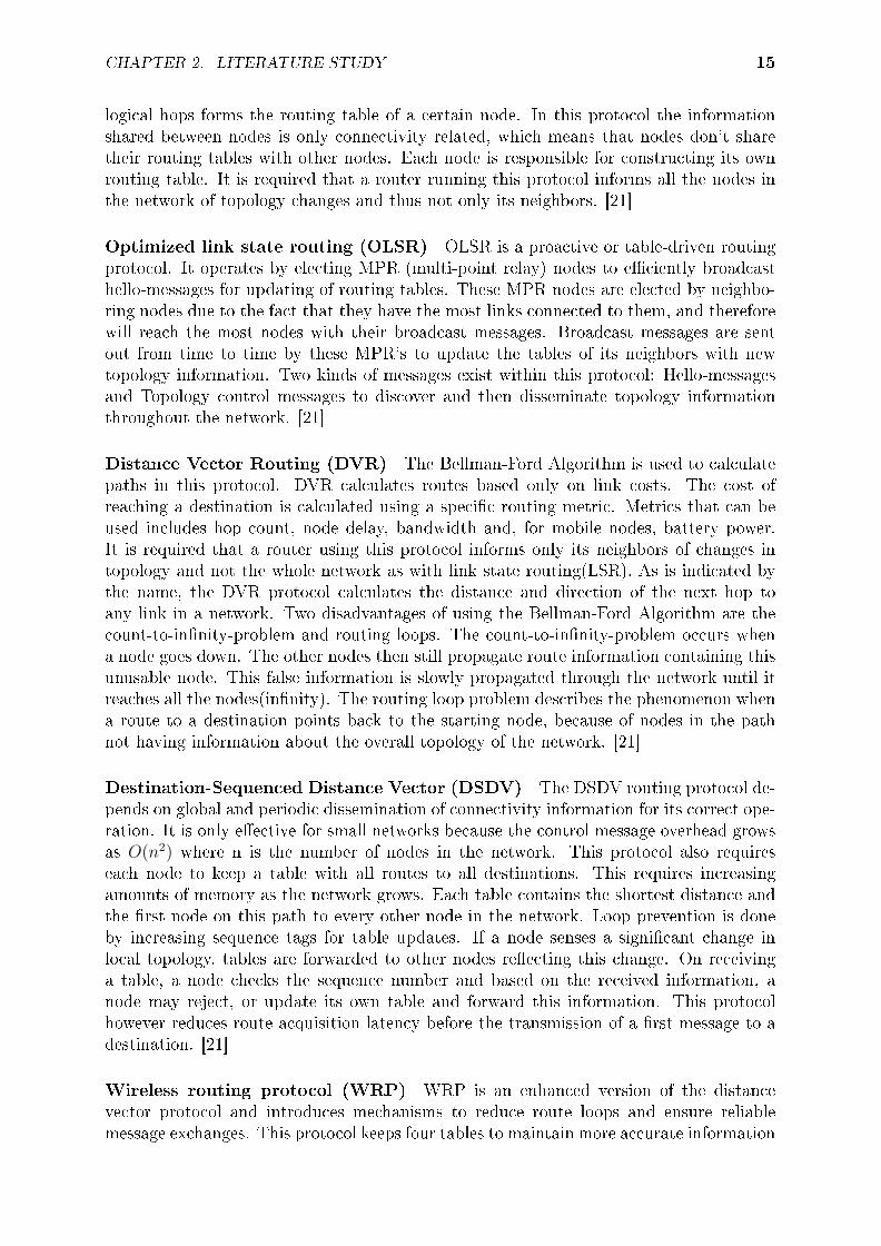
determined by the current position of leopard trap cages in the Cederberg area. Figure3.6 shows all the cage names and coordinates.

CHAPTER 3. THEORETICAL WORK 25
Figure 3.5: Study area showing position of nodes
When all the parameters are kept as described in the two examples above, but to-pography and vegetation information is included as well, only cage pairs Leeuvlak1 andLeeuvlak2, Unnamed cage and Uilsgat bottom cage, and Quintons base and Puntjie cageare connected.
The parameters used are:
Transmit power of 27 dBm
Receive signal strength of -115dBm
Antenna gain of 2 dBi, which implies an omni-directional antenna
Antenna height of 2 m
Total cable loss of 0.5dB
To increase the number of connections, the antenna gain is boosted to 10dBi. Thevalue of the antenna's gain is only varied to show the eect thereof, whilst a practicalomni-directional antenna will never have a gain of 10dBi. Figure 3.7 shows that now onlyBushmanskloof cage, Karukareb cage and Mount Ceder cage are not connected to thenetwork. Mannetjiekloof cage and Vaalkloof cage forms a cluster. Note that the greenlines between nodes show connections.
Increasing the transmit power to 37dBm with the same 10dBi antennae, delivers anetwork with only Bushmanskloof cage and Mount Ceder cage not connected to thenetwork as seen in Figure 3.8. Increasing the transmit power further to 45.4 dBm (35Watt) still does not deliver a network with all units connected. This is not desirable as thebatteries should be as small as possible and last as long as possible. Also one would wantto design as close to an omni-directional antenna as possible and therefore the antennagain should approach 0dBi.
CHAPTER 3. THEORETICAL WORK 26
Cage name Coordinates
Unnamed cage 32.40139S, 19.13667E
Uilsgat bottom cage 32.40806S, 19.15E
Karukareb cage 32.27083S, 19.04778E
Mannetjieskloof cage 32.36611S, 19.34111E
Vaalkloof cage 32.41084S, 19.35028E
Puntjie cage 32.51805S, 19.35389E
Leeuvlak1 cage 32.49139S, 19.38722E
Leeuvlak2 cage 32.50444S, 19.38972E
Sneeuberg cage 32.46083S, 19.16028E
Duiwelsgat cage 32.41139S, 19.08722E
Uilsgat top cage 32.40472S, 19.10611E
Mount Ceder cage 32.62083S, 19.44667E
Bushmanskloof cage 32.13639S, 19.08945E
Quintons base 32.49997S, 19.33583E
Figure 3.6: Cage names and coordinates
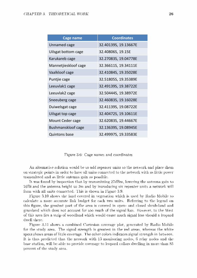
An alternative solution would be to add repeater units to the network and place themon strategic points in order to have all units connected to the network with as little powertransmitted and as little antenna gain as possible.
It was found by inspection that by transmitting 27dBm, lowering the antenna gain to2dBi and the antenna height to 2m and by introducing six repeater units a network willform with all units connected. This is shown in Figure 3.9.
Figure 3.10 shows the land covered in vegetation which is used by Radio Mobile tocalculate a more accurate link budget for each two units. Referring to the legend onthis gure, the greatest part of the area is covered in open- and closed shrub-land andgrassland which does not account for too much of the signal loss. However, to the Westof this area lies a strip of woodland which would cause much signal loss should a leoparddwell there.
Figure 3.11 shows a combined Cartesian coverage plot, generated by Radio Mobilefor the study area. The signal strength is greatest in the red areas, whereas the whitespots shows areas of little coverage. The other colors indicates signal strength in between.It is thus predicted that the network with 13 monitoring nodes, 6 relay nodes and thebase station, will be able to provide coverage to leopard collars dwelling in more than 85percent of the study area.

CHAPTER 3. THEORETICAL WORK 27
Figure 3.7: Network with units tted 10dBi antennae and still transmitting 27dBm
Figure 3.8: Network with units tted 10dBi antennae and transmitting 37dBm

CHAPTER 3. THEORETICAL WORK 28
Figure 3.9: Network with all units connected by using 6 repeater nodes
Figure 3.10: Vegetation information

CHAPTER 3. THEORETICAL WORK 29
Figure 3.11: Combined Cartesian coverage plot

CHAPTER 3. THEORETICAL WORK 30
3.3 Summary
The ICASA specied band for wildlife telemetry tracking was found to be 148 to 152 MHz.The maximum data rate for the parameters specied under channel capacity was foundto be 10kb/sec. Throughput is a function of the communication protocols implementedand will be discussed in chapter 6. The link budget was found to be aected by transmitpower, distance, height of antennas above the ground, wireless channel eects like fading,topography and vegetation. All of this was accounted for by Radio Mobile which predictedthat the network of 13 monitoring nodes, 6 repeater units and the base-station will forma network where all nodes are connected.
In the next chapter we will discuss the details of the MAC and routing protocols thatwere chosen to be most suited for our ad hoc network.

Chapter 4
Communication Strategy
4.1 Introduction
This chapter discusses the MAC (medium access control) - and routing protocols thatwere chosen in chapter 2 for the data link and network layers respectively. Each protocolwill be described on implementation level.
4.2 Medium Access Control protocol description
The data link layer implements the MACAW protocol as discussed in chapter 2. Thisprotocol deals with controlling access to the shared wireless medium. The main tasks ofthe MAC protocol is to:
1. Control access to the channel
2. Distribute bandwidth in a fair manner to all nodes
3. Assure ecient use of the bandwidth
Controlling access to the channel This protocol controls access to the channel bymaking use of a packet-passing scheme between two nodes. Table 4.1 shows all themessages used by the MACAW protocol. The aim of using extra packets other than justDATA packets, is to get a DATA packet to a neighboring node without collisions fromDATA packets from other nodes. This is achieved by keeping nodes that overhear thepacket exchange silent for a period long enough to complete a data transaction betweentwo nodes. The MACAW protocol dictates that a RTS-CTS-DS-DATA-ACK exchange isdone between two communicating nodes. See gure 4.1 for a better understanding. Thesolid lines represents the data intended for the receiver, while the dashed lines representsoverheard packets by other nodes, because of the broadcast nature of the wireless medium.A node that has data to send begins by sending out a RTS requesting to send data toa receiver. Once the receiver receives the RTS, it immediately responds with a CTS,indicating that it is ready to receive data. The transmitter now also knows that thechannel is free and it sends out a DS and DATA packet back-to-back. The DS packetindicates to all nodes adjacent to the transmitter that did not receive the CTS, that a datatransaction is going to take place, so they should not transmit. Upon receiving the datathe receiver will acknowledge it with an ACK packet. Note the dierence in propagationtime for a control packet and a DATA packet, due to the signicant dierence in packet
31

CHAPTER 4. COMMUNICATION STRATEGY 32
Message Meaning Length
RTS Request to Send 12 bytes
CTS Clear to Send 12 bytes
DS Data Send 12 bytes
DATA Data Message 255 bytes
ACK Acknowledgement 12 bytes
RRTS Request to send an RTS 12 bytes
POLL Polling a collar 12 bytes
Table 4.1: MACAW message types
lengths. The data link layer of relay nodes has two focus areas: getting DATA fromleopard collars and sending this data to other relay node using the described protocol.Figure 4.2 exhibits the same message exchange as in gure 4.1, but with relay nodes nowsending out POLL messages to collars to invoke the described protocol. A collar will replywith a RTS only if it has DATA messages to send.
Distributing bandwidth fairly Bandwidth is distributed fairly by making use of arandom back-o scheme. Each node that has data to send, sets a random timer. Onlyafter this time has expired is the node free to try sending data with the protocol packetexchange. If more than one node starts by sending the RTS, it will collide at the receiverand no CTS packets will be sent back. The nodes now restart the contention period byresetting their random timers, but with time-out values chosen from an increased period(back-o value). This will ensure that the chance of two nodes choosing the same back-ovalue will decrease, also decreasing collisions. When no two timers time out simulta-neously, no collisions will occur and the node with the shortest back-o period will rstgain access to the channel. In this case the back-o values at nodes are decreased again.The other nodes receiving RTS, CTS or DS control packets not intended for them willrefrain from transmitting and will only start contending again once the previous exchangewas terminated by an ACK packet. The base station will need the most bandwidth, sinceit has to communicate with all other nodes, while the relay nodes only have to communi-cate data to the base-station. For this reason the base-station is given more bandwidthby keeping its maximum back-o value less than the relay node's back-o values.

CHAPTER 4. COMMUNICATION STRATEGY 33
Transmitter Receiver Neighbour Neighbour
RTS RTS
CTS CTS
DS DS
DATA DATA
ACK ACK
Figure 4.1: MACAW packet exchange between two relays
Ecient use of bandwidth The bandwidth is rstly used more eciently by not usinga scheduling MAC protocol between relay nodes. With MACAW any protocol exchangewill only be done when one relay node has data to send to another, with the exception ofpolling for leopard collars. The bandwidth is also used more eciently by letting nodes indierent regions transmit simultaneously. This means that if a node receives a RTS, butnot a CTS, that its transmission will not interfere with that node's receiver and thereforetwo transmitters can send data to their respective receivers simultaneously. The back-operiods is kept as small as possible and scaled according to the number of nodes in thenetwork so as not to waste time during contention periods.
4.2.1 Detail protocol description
The protocol has three main ows or functionalities which can be seen in gure 4.3 asthe left, right and middle ows. The middle ow shows the states for a normal RTS-CTS-DS-DATA-ACK exchange between two relaying nodes. The left ow shows thetransaction between a relay and a collar node. The right ow shows the states a node goesthrough when overhearing packets not intended for itself. A relay node will perform thetasks of both monitoring for leopard collar presence as well as transferring received datamessages between relay nodes. Note that all broadcast packets like the POLL packet and

CHAPTER 4. COMMUNICATION STRATEGY 34
Relay Collar Neighbour Neighbour
POLL POLL
RTS RTS
CTS CTS
DATA DATA
ACK ACK
DS DS
Figure 4.2: MACAW packet exchange between collar and relay
network broadcast messages are sent without the RTS-CTS-DS-DATA-ACK exchange.Only unicast packets from the network layer are transmitted this way, where DATAmeans any network unicast packet. We will now describe the detail state machine whichforms the MACAW protocol for implementation purposes. The main goal of this statemachine is to progress through the states by sending and receiving packets in an orderlymanner and to return to the right state after a time-out of some sort (a packet got lost)so that protocol exchange can continue in a known state.
Figure 4.3 and 4.4 shows the program structure of this protocol. Note that the protocolfor a wireless relay node and a collar node are slightly dierent. This is because the relaynodes has to poll the collars as well as their basic tasks of forwarding packets betweenrelay nodes.
Communication between two relay nodes: The machine always starts in the IDLEstate. When a message arrives from the upper network layer, it goes into the CONTEND_1state and sets a random back-o timer. When this timer expires it sends a RTS to thenext hop neighbor as specied by the network message and goes to the WFCTS state.If a CTS is received in time, it goes to the XMIT state and sends out a DS and DATApacket back-to-back. If a CTS is not received, the machine tries resending the RTS pa-cket three times before it gives up and sends an error message to the network layer. If an

CHAPTER 4. COMMUNICATION STRATEGY 35
IDLE
CO
NTEN
D_1
WFC
TS
XM
IT
WFA
CK
QU
IET
CO
NTEN
D_2
WFR
TS_1
IDLE
WFD
S
WFD
ATA
IDLE
IDLE
AN
Y STATE
timeo
ut
Send
RR
TS
RTS received
for m
e
recR
TS, CTS, R
RTS, D
S, PO
LL no
t for
me
timeo
ut
timeo
ut/
recA
CK
IDLE
recR
TS
WFD
SC
ON
TEND
_3
WFR
TS_2
timeo
ut
recD
S
Rec
DA
TA/
timeo
ut
timeo
ut
recC
TS x3
recR
TSRec
DA
TA
PO
LL to sen
d
Send
PO
LL
timeo
ut
Send
RTS
recC
TS
Send
DATA
timeo
ut/
recA
CK
time-o
ut
x3
recR
TS
Rec
RR
TS/PO
LLrecR
TS
Msg
to sen
d
Poll tim
er tim
eou
t
Figure 4.3: MACAW for relay nodes
ACK is received after sending out the DATA and DS packets, the network message canbe deleted from the MAC queue. Otherwise it stays on the queue and gets resent whenthe machine times out and goes back to the IDLE state. Looking at the left ow, when areceiving node is in the IDLE state and receives the RTS from the transmitter, it goes tothe WFDS state and sends a CTS back to the transmitter. When the machine times outand no DS packet has arrived, a CTS can be sent up to three times before it times out

CHAPTER 4. COMMUNICATION STRATEGY 36
WFCTS
XMIT
WFACK
IDLE
IDLE
IDLE
Receive POLL
Receive CTS
Send DATA
CTS timeout&& retries > 3
Timeout
Receive ACK
Receive ACK
CTS timeout && retries <=3
Figure 4.4: MACAW for leopard nodes
and goes back to the IDLE state. However, if a DS has arrived, it goes to the WFDATAstate. If no DATA arrives it once again returns to the IDLE state. If DATA arrives, itgoes to the IDLE state, but sends out an ACK packet to the transmitter. A packet ispassed from the data link layer to the network layer only if the destination address of thepacket matches the nodes' network address, or if that eld indicates a broadcast packet.
Communication between a relay and a collar node: The MAC layer sets a timerto regularly time out and send a POLL message. This only happens when the machineis in the IDLE state upon timeout, otherwise it sets a ag and sends the POLL as soonas the machine goes back into the IDLE state. If a leopard is in communication distance,it receives the POLL and sends a RTS back to the relay node. Refer to gure 4.4 forthe collar node's state diagram. It now follows the normal RTS-CTS-DS-DATA-ACKexchange, except that the collar doesn't have to set a random timer before the RTS,it sends the RTS immediately upon receiving a POLL message. Therefore there is alsonot a CONTEND_1 state in this state diagram. On the receiving side, the relay nodes'state machine goes into the CONTEND_3 state when a POLL has to be sent. When therandom timer times out it sends the POLL and goes to the WFRTS_2 state. From hereit follows the same state changes and message passing as discussed above.

CHAPTER 4. COMMUNICATION STRATEGY 37
Quiet times: Any node, including collar nodes, has to refrain from transmitting whenan ongoing transaction is taking place to avoid interference. When a RTS, CTS, RRTS,DS or POLL message is received that is not intended for this node, the node goes intothe QUIET state and sets a dened timer to not transmit for. For instance when a CTSis received, the node has to refrain from transmitting for the period of a DS and DATAmessage. When a RTS is received, it only has to refrain from transmitting for the periodof a CTS. This is to prevent the overhearing node of refraining from transmitting thewhole time if a transaction failed between two nodes. The overhearing node can theninterrupt with its own transmission since the channel is free. It should be noted that inthe case that a RTS is received by an overhearing node while in the QUIET state, it setsa ag to send a RRTS when coming out of the QUIET state. This is to give nodes thatis always caught in others' conversation a change to also transmit. When this happensthe node goes from the QUIET state to the CONTEND_2 state where it sets a randomback-o timer. On expiration it sends out the RRTS packet and goes to the WFRTS_1state. If no RTS is received it simply goes back to the IDLE state. Otherwise it followsthe RTS-CTS-DS-DATA-ACK exchange as discussed above. Table 4.2 through 4.4 showswhich events triggers which actions in the state machine and which conditions should bemet for a certain action to take place. This corresponds with gures 4.3 and 4.4.
Event Predicate Action
Receive POLL State == IDLE • send RTS • State = WFCTS • Set timer for CTS receive
Receive CTS State == WFCTS • Send DS • State = XMIT • Clear timer
DS finished transmit State ==XMIT • Send DATA • State = WFACK • Set timer for ACK receive
Receive ACK State == WFACK • Delete msg from queue • Clear timer • State = IDLE
Receive ACK State == WFCTS • Delete appropriate msg from queue
• Clear timer • State = IDLE
Timer times out State == WFCTS/WFACK • State = IDLE
Timer times out State == WFCTS, txAttempts < 3
• Send RTS • Set timer for CTS receive
Timer times out State == WFCTS, txAttempts >= 3
• State = IDLE • Msg-dropped to network layer
Table 4.2: MACAW event predicate action for Collar
Packet setup When a data stream comes in from the physical layer, it is formattedinto frames by examining the rst byte to determine the packet type. This byte tells the

CHAPTER 4. COMMUNICATION STRATEGY 38
Event Predicate Action
Message to send State == IDLE • Put msg in queue • Set back-off timer • State = CONTEND_1
Back-off timer expires State == CONTEND_1 • Send RTS • State = WFCTS • Set timer for CTS
Receive CTS State == WFCTS • Send DS • State = XMIT • Clear timer
DS finished sending State == XMIT • Send DATA • State = WFACK • Set timer for ACK
Receive ACK State == WFACK/WFCTS • Delete appropriate msg from queue • Clear timer • State = IDLE
Timer times out State == WFACK/WFDATA/QUIET • state = IDLE
Timer times out State == WFCTS, txAttempts < 3 • Send RTS • Set timer for CTS • Increment txAttempts
Timer times out State == WFCTS, txAttempts >= 3 • State = IDLE • Msg-dropped to network layer • txAttempts = 0
Timer times out
State == WFDS, txAttempts < 3 • Send CTS • Set timer for DS • Increment rxAttempts
Timer times out
State == WFDS, txAttempts >= 3 • State= IDLE • rxAttempts = 0
Receive DATA State == WFDS/WFDATA • Send ACK • Sate= IDLE • Clear timer • Send to network layer
Receive RTS State == IDLE/CONTEND_1 • State = WFDS • Set timer for DS • Send CTS • Clear timer
Receive RRTS State == IDLE/CONTEND_1 • Clear timer • State = WFCTS • Set timer for CTS • Send RTS
Table 4.3: MACAW event predicate action for Relay
data link layer what the length of the incoming packet is going to be, so that the receivercan read that correct amount of bytes into a buer for later error checking and correcting.See gure 4.5 for the MAC layer frame structure, which we will now discuss.
The frame is divided into three sections, the preamble, control and CRC (Cyclicredundancy check) sections. The preamble prepares both the transmitting and receivingradios for the important control and CRC bytes to follow. The data slicer settle bytes ischosen as 10101010 to settle the data slicer in the middle. The same way that Manchesterencoding is used to achieve a dc level. It also allows sucient time for the half-duplexradio to switch between receive and transmit mode. The preamble is followed by thereceive USART lock bytes, which triggers the USART to begin reading the bits thatfollows at the correct position to avoid missing the start-of-message bytes. A randomnoise pattern can produce the rst start of message byte ( 01h), so a second byte (7Fh) isadded to prevent the software from triggering. The two bytes are made complementaryto each other to maintain the 50% mark to space ratio [24].
The control section contains all the bytes necessary to constitute a MAC packet. Asmentioned before, the pktKind byte tells the receiver how many bytes to expect. Thesource and destination addresses follows, which are both MAC addresses. Note that sinceonly one byte is used for this purpose, only 28 = 256 nodes can be uniquely addressed. Inall MAC packets the exchange sequence number denotes the current transaction takingplace. The DATA-length eld is to specify the length of a DATA packet if it is brokenup into multiple packets which occurs when the DATA packet is larger than 216 bytes.The BO-value eld is to share with other nodes the current back-o value at this node.
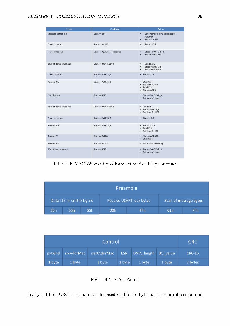
CHAPTER 4. COMMUNICATION STRATEGY 39
Event Predicate Action
Message not for me State == any • Set timer according to message received
• State = QUIET
Timer times out State == QUIET • State = IDLE
Timer times out
State == QUIET, RTS received • State = CONTEND_2 • Set back-off timer
Back-off timer times out State == CONTEND_2 • Send RRTS • State = WFRTS_1 • Set timer for RTS
Timer times out State == WFRTS_1 • State = IDLE
Receive RTS State == WFRTS_1 • Clear timer • Set timer for DS • Send CTS • State = WFDS
POLL-flag set State == IDLE • State = CONTEND_3 • Set back-off timer
Back-off timer times out State == CONTEND_3 • Send POLL • State = WFRTS_2 • Set timer for RTS
Timer times out
State == WFRTS_2 • State = IDLE
Receive RTS
State == WFRTS_2 • State= WFDS • Send CTS • Set timer for DS
Receive DS State == WFDS • State = WFDATA • Clear timer
Receive RTS State == QUIET • Set RTS-received -flag
POLL-timer times out State == IDLE • State = CONTEND_3 • Set back-off timer
Table 4.4: MACAW event predicate action for Relay continues
Preamble
Control
Data slicer settle bytes Receive USART lock bytes Start of message bytes
55h 55h 55h 00h FFh 01h 7Fh
pktKind srcAddrMac destAddrMac ESN DATA_length BO_value
CRC
1 byte 1 byte 1 byte 1 byte 1 byte 1 byte
CRC-16
2 bytes
Figure 4.5: MAC Packet
Lastly a 16-bit CRC checksum is calculated on the six bytes of the control section and

CHAPTER 4. COMMUNICATION STRATEGY 40
appended to the packet to be transmitted.
Data Integrity Cyclic redundancy check refers to a technique to check for the occur-rence of errors in a transmitted message. It only checks for errors and does not correctthem. A checksum is appended to the end of the message to be transmitted. The receivercan use this checksum to determine if errors have occurred and request for the messageto be sent again [28]. The message bits are treated as polynomials with coecients ofeither 0 or 1. The sender and receiver agree in advance on a generator polynomial. Thegenerator polynomial is used to create codewords from the message bits. A properly desi-gned generator polynomial ensures that codewords have good distance properties and aredistributed evenly throughout the code space (see [17] for explanation on code distanceproperties). In general terms CRC generation is based on computing the remainder ofdividing one polynomial by another. For the computation of an r-bit CRC checksum, agenerator of degree r must be chosen. The sender should append r 0-bits to the end ofthe m-bit message. The resulting GF(2) polynomial is of degree m+r-1. This messagepolynomial is then divided modulo-2 by the generator polynomial to produce the remain-der polynomial of degree r-1. The code-vector transmitted is then the m-bit messagewith the r-bit remainder polynomial appended. The receiver on receiving the data canthen compute the checksum of the rst m-bits received, the same way the sender did inusing the agreed upon generator polynomial. If this computed checksum agrees to the lastr-bits received, the transmission was correct [28]. CRC-16 in particular has the followingcharacteristics: According to [27], it can detect
1. All single and double errors
2. All errors with odd-numbered bits
3. All burst errors of length 16 or less
4. 99.997 of all 17 bit errors
5. 99.998 of all errors greater than or equal to 18 bits
CRC-16 is calculated on the packet to determine if bit errors occurred. With MACpackets no forward error correction is done, the packet is only sent again by the transmitteron time-out if bit errors occurred, because the small size of the packet does not justifyadding extra bytes for error correction. Flow control forms part of the implementedcontention protocol.

CHAPTER 4. COMMUNICATION STRATEGY 41
4.3 Routing protocol description
The network layer implements the AODVjr protocol as discussed in chapter 2, whichis a simplied version of the AODV protocol. This protocol deals with the end-to-endcommunication between a source and destination node. The main tasks of the routingprotocol are to:
1. Find the best route between a source and destination node according to some metric
2. Avoid routing loops
3. Maintain this route
4. Handle link breaks
Discovering a route and avoiding route loops Figure 4.7 shows the operations ofthis protocol. When a route is required from node 1 to node 5 where the connection lineshows which are in range of which, a RREQ packet is broadcast and relayed by all nodeson the path to the destination. Node 5 upon receiving the RREQ unicasts a RREP packetback to the originator of the RREQ. The time it takes from the sending of the RREQto the receiving of the RREP is the route acquisition delay. Once that initial delay isover and a route is known to the destination, the source unicasts a DATA packet to thedestination. The destination upon receiving the DATA packet sends an ACK packet backto conrm that it received the data. Each RREQ is uniquely identied by the parameterpair <source address, broadcast id>. Whenever the source node issues a new RREQ,the broadcast id is incremented. When a RREQ is received by an intermediate node, itincreases the hop count and broadcasts the RREQ to its own neighbours. Because a nodecan receive multiple copies of the same RREQ packet, it's source address and broadcastid is checked against a table of already received messages and dropped if it matches oneof the entries. In this way it avoids route loops. In the case of a node forwarding aRREQ, it still keeps track of some information of the message to be able to implementthe reverse and forward path setups, to accompany the eventual RREP. This informationbeing: destination network and MAC addresses, source network and MAC addresses andbroadcast id.
Maintaining a route AODV-simplied maintains its routes by setting a route-life-timetimer once the route is established. This timer is prevented from timing out by packetsbeing received from the destination on the return path. That is RREP's and ACK's resetsthe timer. The route will remain active as long as the timer doesn't time out.
Handling link breaks Figure 4.8 shows what happens during a route break. When alink break occurs, no packets will arrive at the source node and the route-life-timer willeventually time out. This will delete the current route from the source node. When a routeis still required, a new RREQ will be broadcast to set up a new route along a dierentpath. The RREP will be unicast along the new path. A RREQ can be transmitted amaximum of three times if a route is needed, whereafter the network layer will assumethat no route exists to the destination if no RREP is received. This mechanism is to avoidwasting bandwidth and energy. Another attempt at nding a route will only be carriedout if new data messages arrive from a leopard collar.

CHAPTER 4. COMMUNICATION STRATEGY 42
Packet setup Figures 4.9a and 4.9b shows the network layer packets. The networkcontrol packet is 21 bytes long and the network data packet is 262 bytes long. It consistsof a preamble section, control section and CRC section. The preamble which formspart of all packets leaving any node was discussed earlier. In the control section, therst 5 bytes is the MAC layer overhead discussed previously. The netwPktKind bytedistinguishes network control packets from network data packets. Network control kindsis the RREQ, RREP and ACK. The srcAddrNetw and destAddrNetw is both networklayer addresses and being 1 byte long, can also only address 256 nodes' network layers.The broadcastId is used with RREQ packets to uniquely identify each RREQ from acertain source node, such that route loops can be avoided by not forwarding RREQ'swith old broadcastId's. The leopardId uniquely identies from which collar a certainDATA message was received. The messageNum indicates the sequence of DATA messages.The pair leopardId and messageNum uniquely identies a certain DATA message to thebase station. Hopcount indicates how far a message travelled before arriving at the basestation. Both the control and data packets is appended with a 16-bit CRC for errorchecking. Only the data messages has redundant forward error correction bytes to correcterrors. The Read-Solomon error-correction code is used. This code is chosen because itprovides for excellent correction of burst-errors. These errors occur due to heavy rain,lightning or other changes in the atmosphere. The specic Read-Solomon code used wasdesigned to correct up to 13 errors. This maximum is used to provide the data with thebest chance to arrive correctly at the next node. The data section is 216 bytes long andthe data network packet is thus 85% ecient in terms of data ratio to overhead ratio.
Figure 4.6 shows the ow diagram for AODVjr. Once a message is passed from thedata link layer to the network layer, the message is identied by checking the netwPktKindeld. Valid message types are RREQ, RREP, LeopardDATA, ACKnetw and DATA.
Receiving Leopard DATA All data packets that arrive from a leopard collar is for-matted into DATA packets and put in the network queue. If a route is not available tothe destination (base station in this case) a RREQ message is ooded throughout thenetwork in the hopes that it will reach the destination eventually after being relayed byintermediate nodes. A RREP-timer is set within which a RREP should return, otherwiseanother RREQ is sent. However, if a route exists in the forward path table the DATAmessage is sent and an ACK-timer is set within which an ACK should return. If theACK-timer times out before an ACK is received the DATA packet is sent two more timesbefore the network layer establishes that the network is too busy. If that happens, aresend-timer is set to try to resend the data packet in the future.
Receiving a RREP A RREP is a unicast type packet, therefore only the networklayers of the intended intermediate nodes along the return path will receive it. If thenetwork destination address of the packet matches this node's network address, then thisnode was the initiater of a RREQ. The forward path table is now updated with the MACaddress of the packet for implementing a forward path to the base station. The route-life-timer is reset so that the route will remain active for a specied period. A RREP wasreceived, so the RREP-timer can now be canceled such that another RREQ wont be sentagain for the same route. All the messages in the network waiting to be transmitted to thebase station can now be sent one at a time. The network layer implements a FIFO(rstin rst out) queue, so the packets that have been wating the longest in the queue aretransmitted rst.

CHAPTER 4. COMMUNICATION STRATEGY 43
Receiving a RREQ A RREQ is a broadcast type packet, so all nodes' network layerswill receive it. Once it is received, its broadcast id is checked against a table to seewhether it was received previously. If it was, it is immediately deleted. Otherwise thealready received table is updated with this higher broadcast id. Now the return path table
can be updated with the source MAC address of the packet for implementing the returnpath. If this node is the base station(network destination address matches node's) aRREP is sent along the return path, otherwise the RREQ is again broadcast.
Receiving DATA For each DATA packet that arrives at the base station a networklevel ACK is sent back to the originator of the DATA packet, such that the source nodewill know to delete the packet from its queue and send the next packet in queue. ADATA packet is uniquely identied by the <msgNum, leopardID> pair. So if a packetarrives that hasn't before it is stored on the base station's SD-card for downloading by aresearcher onto the computer. If it was received before, this means that the source nodenever got the ACK for the previous packet, so an ACK is still sent back to the source,but the DATA packet gets deleted so no duplicates will exist.
Receiving an ACK If an ACK arrives at an intermediate node, it is simply reversedto the source of the DATA packet. If and ACK arrives at the source node, this meansthat the previous DATA packet got through and the next one can be sent to the MAClayer. The ACK-timer is cleared so the node wont try to resend the same data message.The DATA packet corresponding to the ACK packet's msgNum is now deleted from thesource's network queue.

CHAPTER 4. COMMUNICATION STRATEGY 44
Re
ce
ive
me
ssa
ge
from
MA
C
laye
r
Ch
eck m
essa
ge
typ
e
RR
EQ
Pre
vio
usly
rece
ive
d?
Y
Up
da
te
rece
ive
d
tab
le
De
lete
RR
EQ
N
Up
da
te
retu
rn p
ath
De
stin
ed
for m
e?
Se
nd
RR
EP
(Ba
se
sta
tion
)
Y
Fo
rwa
rd R
RE
Q
(Re
lay s
tatio
ns)
N
RR
EP
De
stin
ed
for m
e?
Re
ve
rse
RR
EP
N
Up
da
te
forw
ard
pa
th
Y
Up
da
te
rou
te life
time
Ca
nce
l
RR
EP
time
r
Se
nd
qu
eu
ed
me
ssa
ge
s
Le
op
ard
DA
TA
AC
K
Sto
re
me
ssa
ge
in
qu
eu
e
Ro
ute
ava
ilab
le?
Fo
rwa
rd
DA
TA
Y
Se
t AC
K
time-o
ut
Sto
re m
essa
ge
in R
RE
Q
qu
eu
e
Flo
od
RR
EQ
Se
t RR
EP
time-o
ut
De
stin
ed
for m
e?
Re
ve
rse
AC
K
N
En
d
Cle
ar A
CK
time
r
De
lete
co
rresp
on
din
g
DA
TA
msg
En
d
En
d
En
d
En
d
En
d
En
dE
nd
N
Y
DA
TA
Ba
se
sta
tion
?
Fo
rwa
rd
DA
TA
En
d
Se
nd
AC
K
NY
Pre
vio
usly
rece
ive
d?
Sto
re o
n
SD
-ca
rd
En
d
N
De
lete
En
d
Y
Figure 4.6: AODV
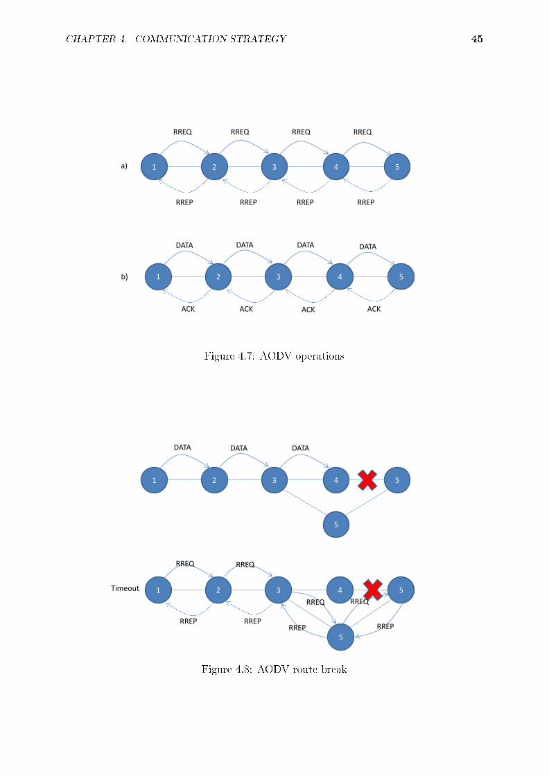
CHAPTER 4. COMMUNICATION STRATEGY 45
1 2 3 4 5
1 2 3 4 5
RREQ RREQ RREQ RREQ
RREP RREP RREP RREP
DATA DATA DATA DATA
ACK
a)
b)
ACK ACK ACK
Figure 4.7: AODV operations
1 2 3 4 5
1 2 3 4 5
5
RREQ RREQ
DATA DATA DATA
Timeout
RREQ RREQ
RREP RREP RREP RREP
5
Figure 4.8: AODV route break

CHAPTER 4. COMMUNICATION STRATEGY 46
Preamble
Data slicer settle bytes Receive UART lock bytes Start of message bytes
55h 55h 55h 00h FFh 01h 7Fh
CRC
CRC-16
2 bytes
Control
pktKind srcAddrMac destAddrMac ESN DATA_length netwPktKind
1 byte 1 byte 1 byte 1 byte 1 byte 1 byte
srcAddrNetw
destAddrNetw broadcastID leopardID msgNum hopCount
1 byte
1 byte 1 byte 1 byte 1 byte 1 byte
Control
(a) Network control packet
Preamble
Data slicer settle bytes Receive UART lock bytes Start of message bytes
55h 55h 55h 00h FFh 01h 7Fh
CRC
CRC-16
2 bytes
Control
pktKind srcAddrMac destAddrMac ESN DATA_length netwPktKind
1 byte 1 byte 1 byte 1 byte 1 byte 1 byte
srcAddrNetw destAddrNetw
broadcastID leopardID msgNum hopCount
1 byte 1 byte
1 byte 1 byte 1 byte 1 byte
Control DATA FEC
DATA
216 bytes
Read-Solomon
26 bytes
(b) Network data packet
Figure 4.9: Network packets

CHAPTER 4. COMMUNICATION STRATEGY 47
4.4 Summary
This chapter described the detail of the implemented medium access control protocolMACAW and the routing protocol AODVjr. In the next chapter we discuss the hardwaredesign of a single node in our ad hoc network.

Chapter 5
Hardware Design
5.1 Introduction
Each wireless station consists of a few integrated hardware components which forms thebasis of an intelligent node in this ad hoc network. First a high level design is doneto determine the functional architecture, then a component selection in which dierenthardware components are considered to yield the best possible solution for the givendesign constraints. Thereafter follows the detail circuit design, cost summary and systemverication of a single node.
5.2 System design
The operational architecture in gure 5.1 shows all units needed to form a working system.Each unit performs a specic task in the system, hence calling them functional units (FUs).The connections between units are the interfaces via which they communicate or interact.Only FU1 and FU4 are designed as part of this thesis. The other functional units areonly drawn to show how FU1 and FU4 t inside the system.
Functional unit 1 Figure 5.2 shows the building blocks of FU1.FU1 is the base station which will reside at the researcher's house for downloading
incoming data packets to a computer. This unit is dependent upon FU4 (relay station)for delivering data packets. FU1 and FU4 interface via radio frequency communication.This unit is controlled by FU1.5 (collar unit) which integrates all the surrounding unitsto form an intelligent node. FU1.1 (RF device) is the functional part which makes theinterface between FU1 and FU4 possible. FU1.2 (secondary storage unit) is needed tostore data packets temporally received from FU4 before they are downloaded onto acomputer (FU2). This is made possible by FU1.4 (serial interface unit) which forms theinterface between FU1 and FU2. FU1.3 (common clock unit) is needed for supplyingthe control units with a common time to time stamp data packets, which will be usedin determining the end-to-end delay of packets as well as route acquisition times. FU1.6(power supply unit) supplies FU1.1, FU1.2, FU1.3 and FU1.5 with power. FU1.8 (PCB)is the structural unit for mounting all units, while FU1.7 (casing) will t all the otherunits inside it for protection against the weather elements.
48

CHAPTER 5. HARDWARE DESIGN 49
FU1 Base Unit
FU2 Computer
FU3 Operator
FU4 Relay Unit
FU5 Collar Unit
FU6 Cage Unit
IF1-4 RF
IF4-5 RF IF4-6 RF IF1-2 Serial
IF2-3 GUI
System boudary
Figure 5.1: System architecture
Functional unit 2 This unit is a computer which interfaces to FU1 via a serial connec-tion for downloading data to the computer's hard disk drive. The computer is loadedwith GUI software for displaying the data.
Functional unit 3 This unit is the researcher who monitors the GUI for received data.
Functional unit 4 FU4 is the relay or milking unit, which polls a leopard collar(FU5) ora leopard cage(FU6) for data. Again these interfaces are radio frequency communicationmade possible by FU1.1 (RF device). FU4 diers from FU1 only by not implementingFU1.4 (serial interface unit) and thus not interfacing to a computer. These units willreside in the eld and will deliver all their data to FU1, therefore obliterating the needfor FU1.5. Figure 5.3 shows FU4's functional block diagram.
Functional unit 5 FU5 is the GPS collar tted to a leopard for tracking the leopard'smovements. This unit is designed by another student and outside the scope of this thesis.
Functional unit 6 FU6 is the camera monitoring unit residing at a leopard cage whichtakes photos of the captured animal and sends it to a relay unit (FU4). The design ofthis unit is also outside the scope of this thesis.

CHAPTER 5. HARDWARE DESIGN 50
FU1.7 Casing
FU1.8 PCB
FU1.5 Control unit
FU1.1 RF Device
FU1.6 Power supply unit
FU1.2 Secondary
storage unit
FU1.3 Common clock unit
FU1.4 Serial interface unit
FU2 Computer
FU3 Operator
IF1-2 Serial
IF2-3 GUI
Figure 5.2: Functional unit 1 architecture
5.3 Component selection
In this section we will consider a few existing o the shelf components for each functionalunit which yields the functionality as described above. We will consider a few choices onthe market and evaluate each one in terms of suitability and cost where applicable.
5.3.1 FU1.1 RF Device
Most importantly the operating frequency has to fall within the ICASA specied rangefor wildlife telemetry tracking, the 148 to 152 MHz frequency band. Table 5.1 shows allthe radios that were found on the market operating in this band. The communicationrange and the data rate has to be maximized while the power consumption should beminimized so that a smaller inexpensive power source can be used. Chapter 3 shows thata transmitter power of 500mW will deliver a feasible range, which means that comparedto a 5W transmitter the power source can be sized 10 times smaller. This eliminates theYS-T86 device. A comparison between the 100mW output power devices (BiM1-151.3-10and FMTR151R) shows that the BiM1-151.3-10 has a higher maximum data rate andcost less. The competition is now between the BiM1-151.3-10 and the BiM1H-151.3-10devices. Both have the same maximum data rate, but with 7dB dierence in transmitpower and R190 price dierence. A power source has to be sized 5 times greater for

CHAPTER 5. HARDWARE DESIGN 51
FU1.7 Casing
FU1.8 PCB
FU1.5 Control unit
FU1.1 RF Device
FU1.6 Power supply unit
FU1.2 Secondary
storage unit
FU1.3 Common clock unit
Figure 5.3: Functional unit 4 architecture
the 500mW transmitter. A network connection comparison between the 100mW and the500mW devices is done in Radio Mobile. Figure 3.9 from chapter 3 shows a networkwith all units connected using six repeater nodes, whilst gure 5.4 shows that six of thecages are not connected to the network anymore. That is Bushmanskloof cage, Karukarebcage, Mannetjieskloof cage, Sneeuberg cage, Leeuvlak1 cage and Mount Ceder cage. Thismeans that at least six extra repeater nodes will be needed, which will cost a lot morethan the price dierence between the two devices added to the price dierence in batterysizes. Therefore the 500mW BiM1H-151.3-10 transceiver from Radiometrix is chosen.
Device Manufacturer Operating frequency Maximum data rate Transmit power Price BiM1h-151.3-10 Radiometrix 151.3MHz 10kbps 500mW R 740.00
BiM1-151.3-10 Radiometrix 151.3MHz 10kbps 100mW R 550.00
YS-T86 Shenzhen Yishi 150MHz 4.8kbps 5W R 1 425.00
FMTR151R Elsema 151.6MHz 4.8kbps 100mW R 1 654.00
Table 5.1: Transceiver options
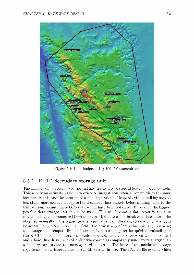
CHAPTER 5. HARDWARE DESIGN 52
Figure 5.4: Link budget using 100mW transmitters
5.3.2 FU1.2 Secondary storage unit
The memory should be non-volatile and have a capacity to store at least 5000 data packets.This is only an estimate as no data exists to suggest how often a leopard visits the samelocation, in this case the location of a milking station. If leopards visit a milking stationless often, more storage is required to download data packets before sending them to thebase station, because more GPS data would have been obtained. To be safe, the biggestpossible data storage unit should be used. This will become a data saver in the casethat a node gets disconnected from the network due to a link break and data have to beobtained manually. This places another requirement on the data storage unit: it shouldbe accessible by a computer in the eld. The easiest way of achieving this is by removingthe storage unit temporarily and inserting it into a computer for quick downloading ofstored GPS info. This argument leads inevitable to a choice between a memory cardand a hard disk drive. A hard disk drive consumes comparably much more energy thana memory card, so the the memory card is chosen. The issue of the maximum storagerequirement is an issue related to the le system in use. The FAT-16 le system which

CHAPTER 5. HARDWARE DESIGN 53
will be used places a restriction of a maximum of 2GB on the storage unit. Knowing thata data packet consists of 216 bytes, 5000 data packets needs 1.08Mb of storage. A 2GBmemory card however provides space for 9.2 million data packets to be stored, whichmeans that virtually no data will ever be lost because it is assumed that a researcherwill have downloaded the data long before the card became full. The secure digital card(SD-card) from San-Disk boasts the advantage over other brands that it uses less power,because it goes into sleep mode automatically when no reading or writing commands isissued in less than 5ms.
5.3.3 FU1.3 Common time unit
The end-to-end delay that a packet experiences in the network is determined by timestamping the packet when it is created at the source node and determining the dierencebetween that time stamp and the current time at the destination node when it is received.For this delay to be accurately determined a common reference time is needed. The globalpositioning system provides a common time to all GPS receivers. In addition of havingaccurate common time, the position of each node will also be known so that researcher'scan nd them easily when they need to be moved. Another reason for using a GPS as bothcommon time and positioning, is for the future implementation of location based-polling.This can save energy consumption in a collar, as a collar only needs to switch on when inthe close proximity of a known milking station.
5.3.4 FU1.4 Serial interface unit
The most common serial interfaces found on modern computers are USB, RS-232 andEthernet. RS-232 has long been the preferred interface for connecting embedded devices toa computer, because of its simplicity. RS-232 is being phased out, as most new computers(especially laptops) don't have external RS-232 ports anymore. Ethernet is a networkport for connecting local area networks and it is common to nd only one such port ona computer. USB is considered as thé interface to connect peripheral devices to a hostcontroller (computer). Usually more than one such port is found on a computer andup to 127 devices can be connected to a single port, which makes it viable to connectyet another device to the computer and not interfere with other connectivity. Manymicrocontrollers have the USB specication already implemented, but that requires thatthe microcontroller also handle the USB stack and the implementation of USB in newdesigns can be time consuming. FTDI (Future technology devices international Ltd)provides a simple solution for connecting your embedded device to a host computer. TheFT232R chip handles the USB stack and converts USART signals from the microcontrollerto USB signals and visa versa. The USB port is then emulated as a com-port withan installed FTDI driver to ease the development of integrating a serial port into newcomputer software, since most computer languages implements a com-port driver. TheUSB specication also allows up to 500mA to be drawn from a single port by an externaldevice. Using this power eliminates the need for an external power socket to power theembedded device. USB delivers 5V regulated power to the PCB, which will be used bythe base station only.

CHAPTER 5. HARDWARE DESIGN 54
5.3.5 FU1.5 Control unit
Knowing the peripherals which will be used in the design, we can specify the controller'stasks in coordinating these peripherals:
1. Send and receive data to and from the radio
2. Store and retrieve received data in non-volatile external memory
3. Swap data between non-volatile and volatile memory
4. Receive GPS and time info from the GPS module
5. Interact with a computer
6. Run MAC and network protocols
7. Manipulate timers
The charging and discharging of the battery will be handled by a separate chargingchip, so no controller intervention is required. The Radio, GPS module and USB interfaceall need USART interfaces for communication. The SD-Card communicates via a master-slave conguration, thus one serial peripheral interface (SPI) port is needed. To freethe microcontroller for protocol related tasks during data transfer between the SD-cardand microcontroller's RAM, a direct memory access (DMA) controller is needed. Thecommunication protocols will need a lot of RAM for temporary storage of incoming andoutgoing packets, routing tables, queues, machine states, FEC coding etc. Therefore themicrocontroller with the largest amount of RAM within a family of controllers shouldbe used. If RAM still proves insucient in the development stadium, primary-secondarymemory exchange can be done, but is not desirable due to speed dierences. Six 16-bittimers in total is needed in the operation of the MAC and Network layers. From theabove list of microcontroller tasks, the following denite features will be required in thechosen microcontroller:
1. Three USART modules for interfacing with the radio, GPS module and USB chip
2. One SPI module for interfacing with the SD-card
3. A DMA controller for data transfer
4. Sucient RAM
5. Six timers for driving protocol events
Other considerations in selecting the correct microcontroller lies in the operating vol-tage, in order that the maximum number of chosen peripherals can be interfaced withoutthe need for voltage level translators.
Table 5.2 shows microcontrollers from each of the existing XMEGA families. Notethat the last letter and numeral denotes a family of microcontrollers. Each microcontrollerchosen is the top of its family because of its amount of RAM being the largest.
The ATxmega32D4 and ATxmega256D3 are disqualied on the basis of having noDMA controllers. The ATxmega128A4 is disqualied on the basis of having only 5 timers.The ATxmega256A3 and the ATxmega384A1 remain and both these microcontrollers meetthe minimum requirements, with the ATxmega384A1 having double the RAM of the
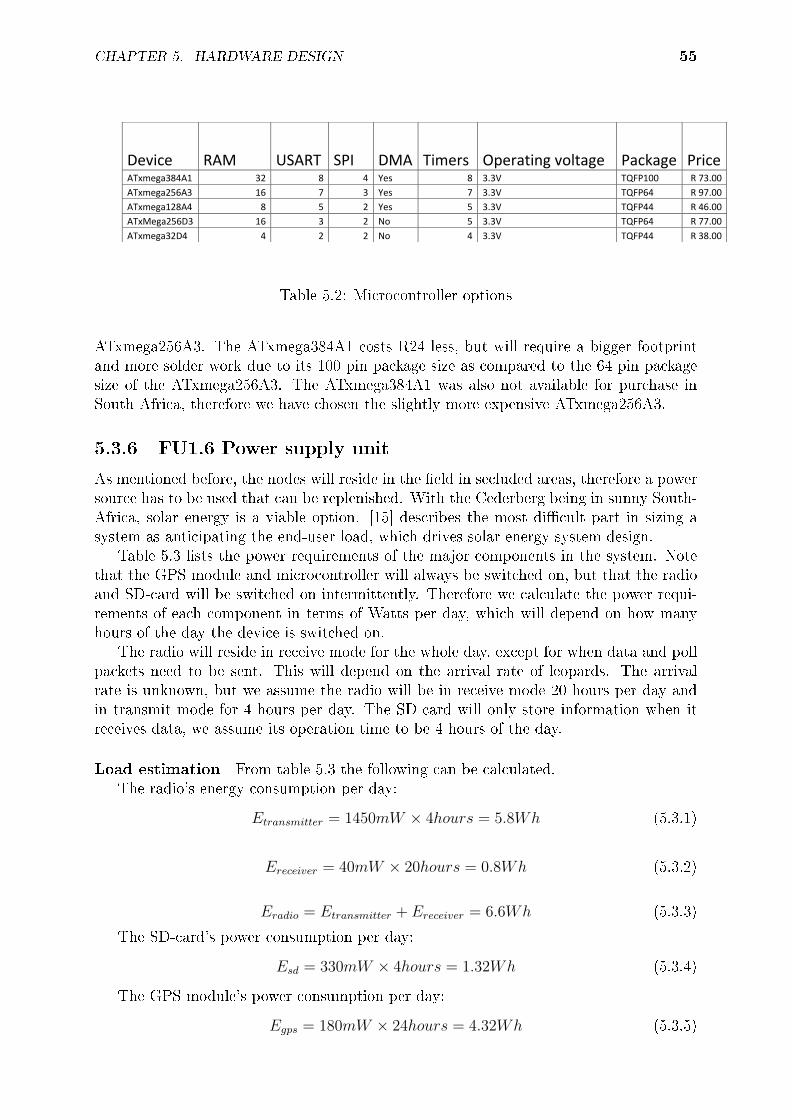
CHAPTER 5. HARDWARE DESIGN 55
Device RAM USART SPI DMA Timers Operating voltage Package Price ATxmega384A1 32 8 4 Yes 8 3.3V TQFP100 R 73.00
ATxmega256A3 16 7 3 Yes 7 3.3V TQFP64 R 97.00
ATxmega128A4 8 5 2 Yes 5 3.3V TQFP44 R 46.00
ATxMega256D3 16 3 2 No 5 3.3V TQFP64 R 77.00
ATxmega32D4 4 2 2 No 4 3.3V TQFP44 R 38.00
Table 5.2: Microcontroller options
ATxmega256A3. The ATxmega384A1 costs R24 less, but will require a bigger footprintand more solder work due to its 100 pin package size as compared to the 64 pin packagesize of the ATxmega256A3. The ATxmega384A1 was also not available for purchase inSouth Africa, therefore we have chosen the slightly more expensive ATxmega256A3.
5.3.6 FU1.6 Power supply unit
As mentioned before, the nodes will reside in the eld in secluded areas, therefore a powersource has to be used that can be replenished. With the Cederberg being in sunny South-Africa, solar energy is a viable option. [15] describes the most dicult part in sizing asystem as anticipating the end-user load, which drives solar energy system design.
Table 5.3 lists the power requirements of the major components in the system. Notethat the GPS module and microcontroller will always be switched on, but that the radioand SD-card will be switched on intermittently. Therefore we calculate the power requi-rements of each component in terms of Watts per day, which will depend on how manyhours of the day the device is switched on.
The radio will reside in receive mode for the whole day, except for when data and pollpackets need to be sent. This will depend on the arrival rate of leopards. The arrivalrate is unknown, but we assume the radio will be in receive mode 20 hours per day andin transmit mode for 4 hours per day. The SD-card will only store information when itreceives data, we assume its operation time to be 4 hours of the day.
Load estimation From table 5.3 the following can be calculated.The radio's energy consumption per day:
Etransmitter = 1450mW × 4hours = 5.8Wh (5.3.1)
Ereceiver = 40mW × 20hours = 0.8Wh (5.3.2)
Eradio = Etransmitter + Ereceiver = 6.6Wh (5.3.3)
The SD-card's power consumption per day:
Esd = 330mW × 4hours = 1.32Wh (5.3.4)
The GPS module's power consumption per day:
Egps = 180mW × 24hours = 4.32Wh (5.3.5)

CHAPTER 5. HARDWARE DESIGN 56
Component Current consumption(mA)
Rated voltage(V)
Resultant power(mW)
Radiotransmitter
290 5 1450
Radio receiver 8 5 40
SD Card 100 3.3 330
GPS module 36 5 180
Microcontroller 14 3.3 46.2
Table 5.3: Component power consumption
Component Input voltage (V)
Output voltage (V)
Efficiency (%)
Solar charging IC
20 6.9 83
3.3V Regulator 6.5 3.3 51
5V Regulator 6.5 5 77
Table 5.4: Regulator eciencies
The microcontroller's energy consumption per day:
EuC = 46.2mW × 24hours = 1.1Wh (5.3.6)
The regulators also dissipate a considerable amount of the total energy. Table 5.4 givesthe eciencies of these components. The microcontroller and SD-card receive energy fromthe 3.3V regulator and the radio and GPS module receive energy from the 5V regulator.All of the energy ows through the solar charger IC. This means that the energy dissipatedby the 3.3V regulator is the voltage drop times the total current owing through it.
The energy dissipated by the 5V regulator is the sum of the power consumptions ofthe GPS module and the Radio times the voltage drop across the regulator.
E5V = (6.5− 3.3)× ((290× 4) + (8× 20) + (36× 24)) = 3.28Wh (5.3.7)

CHAPTER 5. HARDWARE DESIGN 57
The power dissipated by the 3.3V regulator is:
E3.3V = (6.5− 3.3)× ((100× 4) + (14× 24)) = 2.36Wh (5.3.8)
The total energy dissipated by all of the on-board components is thus:
Esubtotal = Eradio + Esd + Egps + EuC + E5V + E3.3V = 18.98Wh (5.3.9)
Because the solar charger IC is a switched regulator and not a linear regulator, itsenergy dissipation is given in terms of eciency. The eciency of the solar charger IC is83 %, which means that it will dissipate 17 % of the total energy itself. Thus it dissipates:
E = 0.17× 18.98 = 3.23Wh (5.3.10)
The total system energy requirement for one day is:
Etotal = Esubtotal/0.83 = 22.87Wh (5.3.11)
Now that the load is known, it is possible to determine the size of the power source.[15] gives the following approximations to estimate the electrical energy expected from asolar panel:
The real capacity of a panel is 15% less than the nominal rating, due to risingtemperatures. The eective capacity being 85% of the nominal capacity.
The expected electrical energy depends on the insolation (peak sun hours) andseason, since insolation levels diers from month to month.
Energy production can be increased by up to 25% if using a sun tracker.
[3] gives the average sun hours for the Western Cape for July(worst) and January(best)as 6.4 hours and 11.3 hours per day. The total number of rainy days during July is 12.Thus it rains roughly a third of the month. We should size the battery supply to last for3 consecutive days.
Thus, the critical design month is July with the least amount of sun hours(6.4). Thebattery should be designed for 3 day's autonomy, not exceeding 50% depth of dischargeand with a round-trip derating eciency of 75%. The load is 22.2Wh.
Battery storage requirement Total daily load Ah requirement = daily energy Watt-hours/battery nominal voltage = 22.87Wh/6V = 3.8Ah
Required battery capacity = (days of autonomy * daily load Ampere-hours) = 11.44AhBut, in order to prolong the life expectancy of the battery, its full charge should not
be used between charging cycles. Fig 5.5 shows that for a battery life of 480 cycles or1.3 years, the battery should only be discharged down to 50% of its capacity. Anotherconsideration is the derating for round-trip eciency (battery eciency), which will betaken as 75%.
Thus, the required battery capacity = (days of autonomy * daily load Ampere-hours)/(derating for round-trip eciency * depth of discharge) = 30.49Ah ≈ 30Ah
Average daily depth of discharge = (total daily load Ampere-hours)/(total batterycapacity) = 3.8Ah / 29.6Ah = 12.8%
Because discharge down to 50% will only happen during the winter months, the lifeexpectancy will be much better than 1.3 years. From 5.5, it will be more than 1200 cycles,which is more than 3.3years.

CHAPTER 5. HARDWARE DESIGN 58
Figure 5.5: Depth of discharge vs life expectancy
Solar panel size estimation We will take the solar panel system eciency as 50%,in accordance with what [15] estimated. The solar panel size is then: total energy requi-red/(peak sun hours * system eciency) = 22.87Wh /(6.4 * 50%) = 7.15Wh
The dierence in insolation levels from Summer to Winter diers. The winter insola-tion levels are only 40% of the maximum (during Summer). Thus the solar panel energyrequirement should be : 7.15Wh/40% = 17.9Wh ≈ 20Wh
System summary
Total Watt-hour requirement: 22.87Wh
Solar panel size: 20Wh
Nominal battery voltage: 6V
Battery capacity: 30Ah
Battery type: SLA deep cycle
Autonomy: 3 days
Average daily depth of discharge 12.8%
Battery life time: More than 3.3 years
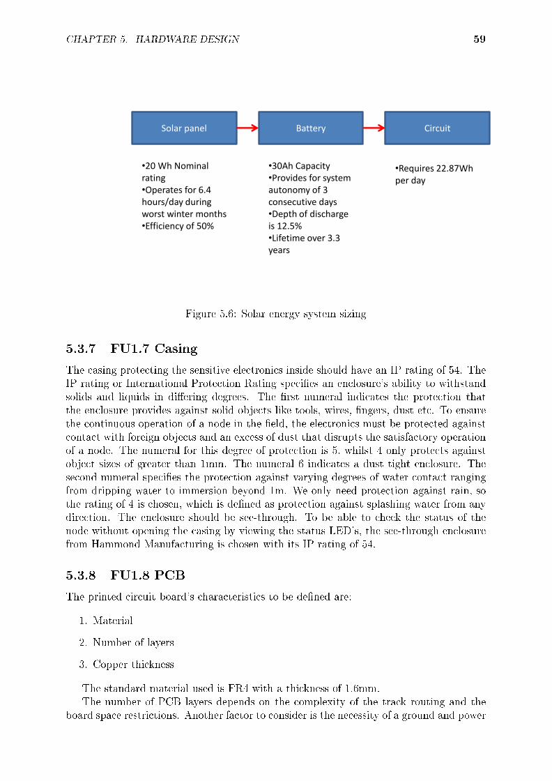
CHAPTER 5. HARDWARE DESIGN 59
Solar panel Battery Circuit
•30Ah Capacity •Provides for system autonomy of 3 consecutive days •Depth of discharge is 12.5% •Lifetime over 3.3 years
•20 Wh Nominal rating •Operates for 6.4 hours/day during worst winter months •Efficiency of 50%
•Requires 22.87Wh per day
Figure 5.6: Solar energy system sizing
5.3.7 FU1.7 Casing
The casing protecting the sensitive electronics inside should have an IP rating of 54. TheIP rating or International Protection Rating species an enclosure's ability to withstandsolids and liquids in diering degrees. The rst numeral indicates the protection thatthe enclosure provides against solid objects like tools, wires, ngers, dust etc. To ensurethe continuous operation of a node in the eld, the electronics must be protected againstcontact with foreign objects and an excess of dust that disrupts the satisfactory operationof a node. The numeral for this degree of protection is 5, whilst 4 only protects againstobject sizes of greater than 1mm. The numeral 6 indicates a dust tight enclosure. Thesecond numeral species the protection against varying degrees of water contact rangingfrom dripping water to immersion beyond 1m. We only need protection against rain, sothe rating of 4 is chosen, which is dened as protection against splashing water from anydirection. The enclosure should be see-through. To be able to check the status of thenode without opening the casing by viewing the status LED's, the see-through enclosurefrom Hammond Manufacturing is chosen with its IP rating of 54.
5.3.8 FU1.8 PCB
The printed circuit board's characteristics to be dened are:
1. Material
2. Number of layers
3. Copper thickness
The standard material used is FR4 with a thickness of 1.6mm.The number of PCB layers depends on the complexity of the track routing and the
board space restrictions. Another factor to consider is the necessity of a ground and power

CHAPTER 5. HARDWARE DESIGN 60
plane. In this design there is no space restrictions as the nished unit will reside in the eldwith plenty of space. Thus the minimum number of layers can be used as all track routingcan be done on a single layer to take up as much space as required. The advantage ofusing less layers is the reduction in cost. The manufacturing cost increases incrementallywith increase in layers. A dedicated ground plane is needed since a component operatingat radio frequency is part of the design. Thus a two layer board will be used with the toplayer the routing and component layer, and the bottom layer the ground layer.
The copper thickness depends on the magnitude of the maximum current a track witha specied width has to carry and the resistance of a certain length of this track. Thisis determined by the power requirements of the design since this is where the highestcurrents ow. The single solar panel allows a maximum current of 1.2A, although theLT3652 solar charger IC allows a maximum current of 2A. We choose to use the maximumcurrent of 2A so that future use of this PCB will not be restricted by the track width.The footprint of the LT3652 IC has a maximum width of 0.42mm per leg. The PCB trackwidth calculator from [4] determines that for a 2A current and 35um copper thickness,the track width has to be 0.781mm. This is larger than what the footprint allows. Usingthe next copper thickness of 70um gives a track width of 0.391mm which is under themaximum allowable footprint width. The 70um copper thickness of the PCB yields aresistance of 0.008Ω per 1 cm, which is an order of 10 smaller than the smallest resistorused (current sense resistor) and will have negligible eect.
To summarize: A double sided FR4 PCB with 70um copper thickness is used formanufacturing.
5.4 Circuit design
Figure 5.7 shows the block diagram for a base station and relay node derived from thesystem level design (and components selection from the previous sections). Communica-tion interfaces between components are also shown. Using this we will discuss the designof the circuit that connects all components in the diagram.
5.4.1 Solar circuit
The LM3652 solar battery charger chip from Linear Technology forms the heart of thiscircuit. The chip is specically designed to regulate the current/voltage relationship ofthe input from the solar panel to tap the optimal power performance from the solar panel.Connectors P8 and P9 on the right and left of gure 5.8 connects the solar panel andbattery respectively. Connecter P10 disconnects the power drain from the power sourcetemporarily to ascertain the correct voltage output in order to avoid damaging the PCB.This is also used as a point to measure the total current drawn from the drain circuit. Theresistors, capacitors and inductor on either side of the LM3652 chip is carefully selectedto yield the correct input voltage, output voltage, maximum current drain and maximumripple current allowed. The chosen solar panel operates at 16.8V giving the input voltageto the circuit. The chosen battery has a nominal voltage of 6V. The battery can be eitheroat or fast charged. With fast charging the voltage across the poles of the battery is sethigher in comparison with oat charging in order to rush more current into the battery ina shorter amount of time. Continuously fast charging a lead-acid battery shortens its lifetime, while the battery can operate an indeterminate length of time using oat charging.The recommended voltage per cell for oat charging is 2.3volts. Thus for the three cell

CHAPTER 5. HARDWARE DESIGN 61
Mic
ro
contro
ller
UA
RT
to
USB
chip
Pro
gra
mm
er
inte
rface
Radio S
ola
r cell
batte
ry
charg
er
circ
uit
Sola
r panelSeale
d L
ead-
Acid
Batte
ry
Ante
nna
SD
Card
USB
In
terface
GPS m
odule
USA
RT
interface
SPI
interface
USA
RT
interface
USA
RT
interface
Vo
ltage tran
slator
Figure 5.7: Hardware block diagram
battery the output voltage from the circuit is 6.9V. LED's D9 and D10 indicates thecurrent state of the charging circuit. D9 will light green when a battery is connected and

CHAPTER 5. HARDWARE DESIGN 62
charging. D10 will light red when some voltage fault occurred.The values of the components surrounding the LT3652 is now determined from equa-
tions given in the data-sheet [7]. The following parameters are used:
Battery oat charging voltage: 6.8V
Solar panel output voltage: 16.8V
Solar panel maximum charge current: 1.2A
Input supply The input capacitor Cin has the function of minimizing voltage glitcheson Vin and reducing ripple current in the charger. A ripple voltage ∆V of 0.1V is recom-mended by the data-sheet.
Cin = Ichg(max) × (Vbat/Vin)÷∆Vin (5.4.1)
= (1.2× (6.8÷ 16.8))÷ 0.1 = 4.85uF
We choose a standard capacitor value of 10uF, yielding an even smaller ripple voltage.
Charge current programming Programming the maximum charge current is donethrough a very small valued resistor called a current sense resistor.
Rsense = 0.1÷ Ichg(max) (5.4.2)
= 0.1÷ 1.2 = 0.083Ω
A standard 0.082Ω current sense resistor is chosen.
Inductor selection The criterion for selecting the inductor depends on the maximumripple current created in that inductor. The ripple current is typically set to 25% of themaximum charge current. Thus ∆Iripple = 0.3A
L = (10×Rsense/∆Iripple)× Vbat × (1− (Vbat/Vin)) (5.4.3)
= (10× 0.082÷ 0.3)× 6.9× (1− (6.9÷ 16.8)) = 11.1uH
We chose the standard 22uH which yields even smaller ripple current. Another impor-tant selection criterion for and inductor is the saturation current which should be equalto or exceeding the maximum current in the inductor.
Isaturation ≥ (1 + ∆Iripple/2)× Ichg(max) (5.4.4)
≥ (1 + 0.3÷ 2)× 1.2 ≥ 1.38A

CHAPTER 5. HARDWARE DESIGN 63
Rectier diode selection The rectier diode has to meet forward voltage drop, reversevoltage and maximum current specications.
The maximum reverse voltage of the diode has to be greater than the maximum outputvoltage of the solar panel of 20.5V. The forward voltage drop has to be as small as possible,to yield the lowest power loss and thus the greatest eciency. The maximum current isdetermined as:
Idiode(max) > Ichg(max)×((Vin(max)−0.7×Vbat)/Vin) (5.4.5)
> 1.2× ((20.5− 0.7× 6.9)÷ 20.5) > 0.92A
The MBRS340 schottkey diode meets these criteria.
Battery oat voltage programming The oat voltage programming is done by asimple resistor divider circuit. The two equations used to determine the two resistorvalues are:
R1 = (Vbat × 2.5× 10⁵)/3.3 (5.4.6)
R2 = (R1 × (2.5× 105))/(R1 − 2.5× 10⁵) (5.4.7)
R1 = 6.9 × 2.5 × 105 ÷ 3.3 = 522.7kΩ Choose R1 to be 530kΩ so that the value canbe approximated by a 510kΩ and a 20kΩ in series.
R2 = (530k × 2.5× 105)÷ (530k − 2.5× 10⁵) = 473.2kΩ which can be approximatedby a 470kΩ and a 3kΩ resistor in series. The tolerance on the resistor values is 0.1%, sothe oat voltage should be reasonably accurate.
The output voltage now yields 7V, which is a bit higher, but still under the batterymanufacturer's specication for cycle charging (7.2V).
Input supply voltage programming The input voltage is also programmed by aresistor divider network. This is done so that the input voltage regulation loop has areference for the voltage used to drive the circuit for the optimal performance of the solarpanel by regulating the voltage/current characteristic. We choose Rin2 to be 100kΩ anddetermine Rin1.
Rin1 = ((Vin − Vforward(D1)−2.74)×Rin2)/2.74 (5.4.8)
Rin1 = (16.8− 0.5− 2.74)× 100k ÷ 2.74 = 494.9kΩ
5.4.2 Power circuit
Linear regulators Reg113-5 and Reg113-3.3 from Texas Instruments respectively sourcethe 5V and 3.3V components on the PCB. Both regulators include capacitors rangingfrom 1000uF to 10nF to lter out low and high frequency components from the solarcharging circuit, since the charging circuit uses a switching regulator and thus adds rippleto the power rail. The 1000uF also serves as a power reservoir in case the peak powerdrawn from the PCB spikes, such that the voltage will not drop, but current can be drawnfrom this capacitor. Header P1 allow manual switching of power source between the 6Vfrom the battery or the 5V from the USB port. This is so that a single PCB design couldbe used for both the base station and the relay stations.

CHAPTER 5. HARDWARE DESIGN 64
5.4.3 Transceiver interface
Figure 5.10 shows the radio with antenna connection and data connections to the micro-controller. The antenna connection is an SMA screw connector, connected from the radioRF pin to the SMA connector by a 50Ω microstrip line to match the 50Ω impedanceantenna. The width of this strip line was calculated knowing the copper thickness on thePCB to be 70µm and distance between the strip line and ground plane as dictated by thethickness of the PCB insulator material as 1.6mm. The relative permittivity of the FR4material is 4.9. The calculation was done with the web-base calculator from [22] and thewidth was calculated to be 2.74mm. There is however only space for a 2.4mm microstripline between the pins of the radio. This yields a 54.4Ω characteristic impedance on themicrostrip line, which will have some reections.
The radio's power rail has a series ferrite bead, which is a magnetic device that at-tenuates all frequencies in the MHz range by dissipating them acting as a 30Ω resistor.This stops spurious frequencies on the power rail from introducing interfering noise to theradio.
The radio and micro-controller work at dierent logic levels. To interface the two, avoltage level translator is introduced to switch signals from 3.3V to 5V. This is howeveronly done on the transmitting side, as the receiving side of the radio outputs 2.5V signalsdirectly to the microcontroller, which is still above the minimum level recognizable by themicro-controller. A line lter is also put on the transmitting line from the micro-controllerto the radio to reduce switching noise. Small sized capacitors is put on all components'power lines to reduce the eect of a sudden voltage drop.
5.4.4 Programmer interface
The programmer uses the universal JTAG interface to program the microcontroller. Thisinterface uses 5 communication lines, power and ground lines. The 5 communication linesare data-in, data-out, clock, mode select and reset.
5.4.5 Serial interface
The FT232RL chip from FTDI converts USART signals from the microcontroller intoUSB signals and back for communication between a computer and the microcontroller.LED D4 and D5 respectively signals a transmit and receive event. The external powerswitch cuts power to the PCB when the computer goes into sleep mode to comply withthe USB specication of not drawing more than 500µA from the port. Header P2 canbe manually switched such that the PCB draws power from either the USB port or the5V regulator coming from the battery, depending on whether the PCB is used as a basestation or relay station. The ferrite bead on the USB port's power line dissipates unwantedhigh frequency noise.
5.4.6 GPS interface
The GPS module can communicate by either RS232 or TTL signals. For convenientlyinterfacing directly to the microcontroller's USART port, the 3.3V TTL interface is used.The GPS module inputs 5V power, but has an on-board 3.3V regulator for the TTLsignals to and from the microcontroller.

CHAPTER 5. HARDWARE DESIGN 65
5.4.7 SD-card interface
The SD-card communicates via the microcontroller's SPI port, which uses four lines. Achip select(CS) for activating the SD-card. A Clock signal and two data lines: master-in-slave-out(MISO) for communication from the SD-card to the microcontroller and master-out-slave-in(MOSI) for communication from the microcontroller to the SD-card. The50kΩ resistors connected between these lines and the 3.3V power rail, ensures that thelines don't oat when inactive and thus don't consume unnecessary power.
5.4.8 Microcontroller circuit
The microcontroller is at the heart of the PCB, coordinating the operation of all theperipheral modules. All communication connections are made to and from the microcon-troller. The reset circuit, consisting of a switch and a resistor, draws the microcontroller'sexternal reset line to ground, to signal a reset event. LED's D1 and D1 signals transmitand receive events for the radio. An external crystal is connected as clock source clockingat 7.3728MHz. This frequency is specically chosen so that the USART module on themicrocontroller can accurately operate at the standard baud rates by dividing the crystalfrequency without a remainder. 100nF capacitors is placed on all the power to groundconnections to keep the power rail always high at 3.3V.
5.4.9 PCB layout
The most important consideration for the layout is to keep the fast switching digitaldevices and power circuits far away from the analog radio. This is done to minimizeinterference on the radio channel. Digital logic ground currents can also interfere withanalog circuitry, therefore the two dierent currents should be isolated. One approachis to split the ground plane of the analog part and the digital part and only connect itat one point, since a common reference is still needed. However, this causes problemswhen routing traces over the split in the plane. This will mean that the return digitalcurrent will still have to ow through an analog ground plane or visa versa. Digital groundcurrents, which is usually high frequency, want to return directly underneath the signaltrace and therefore have no desire to ow through analog portions of the ground plane[23]. It is important to separate the analog and digital sections and keep in mind wherereturn currents ow.
5.5 Cost
Table 5.5 shows the total cost of one stand-alone wireless station. The costly singlecomponents are the radio, battery, solar panel, microcontroller, GPS-module, SD-Cardand PCB.
5.6 System verication
The system consists of ve mayor functional blocks. That is the radio communication,computer communication, GPS communication, SD-card storage and power supply. Thefollowing paragraphs describes the verication tests that was performed on each block.

CHAPTER 5. HARDWARE DESIGN 66
Component Description Price
Radio Transceiver BiM1H-151.3-10 R 741.00
Antenna ZARA-130 R 340.00
Antenna mount Dropper R 100.00
Antenna connectors Male and female R 35.00
Microcontroller XMEGA-256-A3 R 200.00
Battery Sealed Lead Acid 6V 12Ah R 110.00
Solar panel 20 Watt R 640.00
Solar battery charger chip LT3652 R 53.00
USART to USB chip FT232RL R 36.00
USB Connector mini B R 8.00
GPS Module LEA-4P-SMART R 375.00
SD-Card San Disk 2Gb R 115.00
SD- Card Connector Standard type R 25.00
Voltage level translator TXS0104 R 10.00
Linear Regulator 5V REG113EA-5 R 32.00
Linear Regulator 3.3V REG113EA-3.3 R 32.00
Crystal Oscillator 7.3728MHz R 5.00
T-Filter surface mount R 10.00
p-channel mosfet IRLML6401 R 3.00
Power Inductor 2A R 12.00
Push-button surface mount R 4.00
Miscellaneous Diodes, LED's, resistors, capacitors, connectors R 500.00
PCB Manufacturing Double sided, FR4, 70um R 572.00
Enclosure See through IP54 rating R 90.00
Total: R 4,048.00
Table 5.5: Total cost of one station
Radio Communication We verify the following for radio communication:
1. Operating frequency
2. Transmit power
3. Data rate
4. Two-way communication
The carrier frequency was veried to be 151.3MHz by means of a spectrum analyzer. Itrequires the RF pin of the radio to be connected through an attenuator to avoid exceedingthe spectrum analyzer's maximum input power. The radio was transmitting 1's and 0'sinterchangeably. The spectrum analyzer showed two maxima on either side of the carrierfrequency, representing the two frequencies used to modulate 1's and 0's. 151.3MHz wasthe middle frequency.
If the transmit power is lower than rated or there is too much reection in the connec-tors and antenna, the expected range will be decreased. As shown in chapter 6, a radiorange test was done in the Cederberg and yielded a maximum distance of 12.42km. Thisis in accordance with the data sheet, stating that a radio link of more than 10km can beestablished.

CHAPTER 5. HARDWARE DESIGN 67
The maximum data rate possible with a bit error rate of one in a million should be 10kbits/s. This was tested by the micro-controller clocking out data packets to the Radio-USART port at 10 000 baud. 100 % of 200, 64-bit packets was received correctly withthe two antennas 20 meters apart.
Verication of two-way communication is the same as the data rate test, only thistime the receiver was made to transmit and the transmitter to receive.
Computer communication The PCB was connected to the computer through a USBcable. A set of characters was sent through the USART connected to the USART to USBchip. All characters was received correctly by inspection through hyper-terminal.
GPS communication Time information was veried against a watch and GPS infor-mation against a Garmin GPS handheld device.
SD-Card Storage Text les with known data was stored by the microcontroller on theSD-card which implements a FAT-16 le system. The SD-Card was removed and read ona computer running Windows. All data was read correctly. Text les were again storedby the computer on the SD-card. The microcontroller read the les and sent it throughthe USB interface to the computer's hyperterminal to be veried correctly.
Power We verify the following aspects of the power module:
1. Charge voltage
2. Charge current
3. Regulator voltages
The solar battery charger circuit was designed to charge a battery at 6.8V with acharging current of 1.2A. Both these values were obtained correctly with a multimeter.The 5V and 3V regulators should of course deliver that respective voltages, which it did.
5.7 Summary
This chapter described the system level design of both a base station and relay stationsfor use in the leopard tracking project. Each block of the system design was discussed interms of its functional use. The selection of hardware components was discussed with thefollowing results: the BiM1H-151.3-10 transceiver from Radiometrix was chosen as RFcommunication unit, the 2GB SD-card from San-Disk was chosen as secondary storageunit, the LEA-4P GPS module from RFDesign was chosen as both the common clockunit and positioning unit, the FT232R chip from FTDI was chosen as computer serialinterface unit for the base station, the ATxmega256A3 from Atmel was chosen as controlunit, the LT3652 chip from Linear Technology was chosen as the solar battery charger forthe relay stations and see-through enclosures was chosen from Hammond Manufacturingfor all stations. Detailed calculations showed the power supply sizing design for a relaystation using a solar panel and SLA battery. All units was veried to work correctly. Thetotal cost of one stand-alone station was calculated to be R4048.
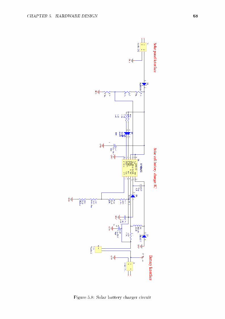
CHAPTER 5. HARDWARE DESIGN 68
Figure 5.8: Solar battery charger circuit

CHAPTER 5. HARDWARE DESIGN 69
Figure 5.9: Power circuit

CHAPTER 5. HARDWARE DESIGN 70
Figure 5.10: Transceiver circuit

CHAPTER 5. HARDWARE DESIGN 71
Figure 5.11: JTAG interface
Figure 5.12: USB interface

CHAPTER 5. HARDWARE DESIGN 72
Figure 5.13: GPS interface
Figure 5.14: SD-card interface

CHAPTER 5. HARDWARE DESIGN 73
Figure 5.15: Microcontroller circuit

Chapter 6
Experimental investigation
6.1 Introduction
The aim of this chapter is to give results in terms of what the hardware and therebyformed network is capable of. It is important to give an idea of the performance of thenetwork so that the end-user can know what to expect from the network. In experimentingwith a range of parameters for each test, it is possible to determine the limits or boundsof the system, so that one can operate the network well beneath it to achieve reliabilityof operation.
6.2 Error performance of radio
6.2.1 Motivation
It is necessary to determine the optimal baud rate at which the radios can communicatefor a certain packet error rate. Literature suggests that a higher baud rate will introducemore errors, however [24] determined a baud rate of 9600bps to be optimal for a similarBiM-UHF transceiver from Radiometrix, while a lower baud rate of 4800bps performedworse. It is attempted to do the same experiment, but for the BiM-VHF radio transceiver.The BiM1 transceivers' data sheet suggests that the lower the baud rate the more rangethe radios have. Baud rate inuences the end-to-end delay of packets, which determinesthat for a lower baud rate, the network will become congested faster.
6.2.2 Experimental setup
The baud rate of communication is changed from 600bps to 9600 bps. A dummy packetwith 8 bytes of data is sent 500 times, and the receiver stores every packet that wasreceived without error. Each measurement is done 3 times and the average packet errorrate is used.
6.2.3 Results
Figure 6.1 shows that for a signal strength of -95dBm(which is a fairly strong signal) thebaud rate does not inuence the packet error rate i.e. there is no loss of packets. With asignal strength of -108dBm(close to the receiver threshold) for the highest and the lowestbaud rates, the performance is worst, while for 1200, 2400 and 4800, the packet error rate
74

CHAPTER 6. EXPERIMENTAL INVESTIGATION 75
is eectively the same. At 4800bps the packet error rate is 5% less than the maximum of9600bps.
0
2
4
6
8
10
12
14
16
600 1200 2400 4800 9600
PER (%)
Baud rate (%)
Packet error rate versus Baud rate
-108dBm
-95dBm
Figure 6.1: Baud rate vs PER
6.2.4 Interpretation
A good choice for communication speed would be 4800bps, as its performance is the sameas 1200 bps, with the advantage that data will be sent four times faster.
6.3 Throughput
6.3.1 Motivation
Network throughput is dened as "..the average rate of successful message delivery over acommunication channel" [30]. For this network it is important to know the throughput atthe base station, since the base station is the sink, meaning all nodes send their packetsto the base station. We distinguish between maximum theoretical throughput, peakmeasured throughput and maximum sustained throughput. The maximum theoreticalthroughput is closely related to the data rate of the channel, but also taking overhead intoaccount. The peak measured throughput is the instantaneous throughput measured overa very short period of time, while the maximum sustained throughput is measured andaveraged over a longer period of time. The maximum throughput is the minimum messagearrival rate that will cause the delay of packets in the network to increase to innity

CHAPTER 6. EXPERIMENTAL INVESTIGATION 76
and thus make the system unstable [30]. We are interested in the maximum sustainedthroughput, since we want to nd the message arrival rate at which the network becomesunstable and increases delay to innity. When the delay goes to innity, the throughputgoes to zero. We do this by measuring the delay that packets experience in the network,since delay is the inverse of throughput.
6.3.2 Experimental setup
Five test units were built for testing the protocols and measuring the performance thereof.One unit has to act as a base station, while at least one has to act as a leopard collar andthe rest should be relay stations for testing the multi-hop. Figures 6.2 and 6.3 show thetwo topologies that has been created using the ve units.
Relay 1 Base-station
Leopard
Relay 2 Relay 3
Figure 6.2: Network topology 1
Base-station
Leopard 1
Relay 1 Relay 2
Leopard 2
Figure 6.3: Network topology 2
Figures 6.4 and 6.5 show screen captures of the two topologies as done in OMNET++with the MIXIM framework. The simulation software can be found on the enclosed DVD.
To measure the end-to-end delay that a packet experiences in the network, it is neces-sary to time stamp the packet at creation time and subtract that time from the time thatthe packet arrives at the base station. Once 50 packets have arrived, their end-to-enddelays are averaged. This is done for both simulation and measurements to be able tocompare the results to see how accurate the simulation models the network.

CHAPTER 6. EXPERIMENTAL INVESTIGATION 77
Figure 6.4: Screen capture of topology 1 as done in OMNET++
Figure 6.5: Screen capture of topology 2 as done in OMNET++
6.3.3 Results
Figure 6.6 shows the results for topology 1. The increase in delay at the increase inmessage arrival rate is to be expected, since the wireless channel has a nite capacity.Once messages arrive from a leopard collar faster than the network can send them to thebase station, packets start queuing up at the rst relay station. The average increaseddelay portrays the waiting time at the relay station's network queue. Notice how closelythe simulation values resemble the actual measured values(all measured values fall withinthe standard deviation of the simulation values). Notice also how the standard deviation

CHAPTER 6. EXPERIMENTAL INVESTIGATION 78
of the simulation values starts to increase at the increase in message arrival rate. This canbe explained because of the network that becomes unstable with delay values approachinginnity.
0
50
100
150
200
250
300
350
400
0 0.05 0.1 0.15 0.2 0.25
End
-to
-en
d D
ela
y (s
)
Message arrival rate (packets/sec)
End-to-end Delay vs Message arrival rate
Simulation
Measured
Figure 6.6: End-to-end delay for topology 1
Figures 6.7 and 6.8 shows the dierence between a packet arrival rate that leads to sus-tained throughput and one that approaches zero because the end-to-end delay approachesinnity.
Figure 6.9 shows the end-to-end delay for topology 2. The same trend is observedas with topology 1, however here the end-to-end delay does not approach innity as fastas with topology 1. This is because the parameters for both were kept the same, buttopology 1 has only 2 hops and thus the packets spend less time in the network.
6.3.4 Interpretation
At a message arrival rate of 0.2 packets per second (1 packet in 5 seconds), the networkbecomes congested and the throughput at the base station approaches zero (end-to-enddelay approaches innity). The maximum message arrival rate should thus be 0.1 packetsper second (1 packet in 10 seconds). This is feasible, since it is expected that the leopardarrival rate will be once per day with the collar sending a maximum of 2 data packets.One position x takes 4 bytes and one data packet allows for 223 bytes to be sent. Thusa total of 111 position xes will be sent over two data packets. This will take roughly 40seconds (20 seconds per packet) to send through 3 hops. The message arrival rate of 0.1packets per second will give the network enough time to deliver leopard packets to the

CHAPTER 6. EXPERIMENTAL INVESTIGATION 79
Figure 6.7: End-to-end delay over time lapse for 0.1 packets per second arrival rate
Figure 6.8: End-to-end delay over time lapse for 0.2 packets per second arrival rate
base station without becoming congested. A photo will be approximately 10kB, so has tobe sent in 45 packets. The leopard cage station can be made to do ow control in whichit sends 0.1 packets per second, so from Figure 6.6 it will take 20 seconds per packet and15 minutes for the entire photo to arrive at the base station. Comparing this to the 3hours and more it takes to manually go and download a photo in the eld (depending onthe location of the cage), the network provides a much faster solution.

CHAPTER 6. EXPERIMENTAL INVESTIGATION 80
-5
0
5
10
15
20
25
30
35
0 0.05 0.1 0.15 0.2 0.25
End
-to
-en
d D
ela
y (s
)
Message arrival rate (packets/sec)
End-to-end Delay vs Message arrival rate
Simulation
Measured
Figure 6.9: End-to-end delay for topology 2
6.4 Route acquisition delay
6.4.1 Motivation
The route acquisition delay is the time it takes to discover a route to the destination (basestation) once a leopard packet has arrived at a relay station. It is necessary to see whatthe eect on the number of hops is, to determine what the delay would be from the timethat a packet arrives from a collar to the time that the rst packet arrives at the basestation.
6.4.2 Experimental setup
A timer is started once a RREQ is broadcast and stopped once a RREP arrives in replyto that RREQ. Fifty of these measurements are made and the average taken to yieldaverage route acquisition delay. This is measured with an increase of one hop each time.The maximum number of hops that the ve node network can form is 3 (leaving one forthe base station and one for a leopard collar). The simulation is run for more than threehops however, to show the trend in the route acquisition delay.
6.4.3 Results
The graph in gure 6.10 shows linear increase with an increase of about 2.5 seconds foreach hop added. The measured results follows the simulation results closely. The standard

CHAPTER 6. EXPERIMENTAL INVESTIGATION 81
deviation is rather large, which reects the contention that RREQ packets have with RTSand POLL packets from other nodes. Sometimes RREQ packets goes through withoutany collisions (yielding a small value for route acquisition delay) and other times theycollide with RTS and POLL packets, requiring a relay station to send out another oneand adding more delay to a route being found (yielding a large value for route acquisitiondelay).
-5
0
5
10
15
20
25
0 1 2 3 4 5 6 7
Ro
ute
acq
uis
itio
n d
ela
y (s
)
Number of hops
Route acquisition Delay vs Number of hops
Simulation
Measured
Figure 6.10: Route acquisition delay
6.4.4 Interpretation
Longer routes will have a greater impact on the initial delay that packets will experienceif no route exists to the base station. The greatest number of hops in the network is 4(refer to gure 3.9 in chapter 3), so this should be about 7.5s as seen on gure 6.10.
6.5 Range tests - eldwork
6.5.1 Motivation
In order to determine the feasibility of a land-based radio network in an environment likethe mountainous Cederberg, it was necessary to do actual eld tests. This can now becompared with the theoretical and simulation results from Radio Mobile from chapter 3 todraw a better model for this area and predict the link quality at other sites not measured.

CHAPTER 6. EXPERIMENTAL INVESTIGATION 82
6.5.2 Experimental setup
The range tests are done incrementally. Two radios are placed rst 100m apart, checkedfor communication and then the distance between the two gets incremented and againchecked for communication. A GPS is used to mark the spots where the antennas areplaced so that it can be plotted on Radio Mobile to compare the results. First line-of-sighttests are done, and later non-line-of-sight tests. For the non-line-of-sight test two radiosare placed on either sides of a hill where Radio Mobile predicts a working communicationslink.
6.5.3 Results
After having success with some minor distances, a link of 2.6km is established with successas depicted by gure 6.11.
Figure 6.11: 2.6km line-of-sight link
Next a distance of 10.43km is attempted as depicted in gure 6.12 with success. Notethat this agrees with the data sheet for the used radio, which suggests that a line-of-sightradio link of over 10km can be established.
Figure 6.12: 10.43km line-of-sight link
Next a longer link is attempted where the line of-sight-path just scrapes the top of ahill as depicted in gure 6.13 with moderate success as only half of the packets sent camethrough. The distance is 12.42km.
Figure 6.13: 12.42km link

CHAPTER 6. EXPERIMENTAL INVESTIGATION 83
Now two non-line-of-sight tests are done, one long-distance and one short-distance.Figure 6.14 shows the hill to the right of the picture blocking the direct communicationlink. Radio Mobile does predict a strong link of 21.1dB beyond the receive signal strengthmargin. No communication is established however.
Figure 6.14: 10.29km non-line-of-sight link
For the short distance line-of-sight link, a distance of 3.73km is used between radiosas depicted by gure 6.15 without success. Again Radio Mobile predicted a strong link.
Figure 6.15: 3.73km non-line-of-sight link
6.5.4 Interpretation
For reliable communication with a carrier frequency of 151.3MHz, direct line-of-sight linkshave to be used, because with the non-line-of-sight links no communication was establi-shed. Radio Mobile's predictions seem to be inaccurate for non-line-of-sight links. Thisis ascribed to ground reections and scattering which Radio Mobile does not take intoaccount. It is desired to have a model that resembles the eld tests more closely, so thatRadio Mobile can be used to do accurate predictions of links for which eld tests werenot done due to time restrictions. Radio Mobile is set up to predict only where line-of-sight links will be feasible, thus using the terrain data to ignore links where any obstaclesblock a direct line-of-sight. This is done by introducing extra losses to account for theseunaccounted eects in Radio Mobile. This changes the predictions made in chapter 3considerably, because using the new line-of-sight-only-model, Bushmanskloof cage, Karu-kareb cage, Mannetjiekloof cage, Vaalkloof cage, Leeuvlak1 and 2, and Sneeuberg cageare not connected to the network. This is to be expected as all of these cages lies indips, so more repeater units should be placed on strategic places to connect them to thenetwork as well.
Figure 6.16 shows the network for the line-of-sight model in Radio Mobile. Threeextra units are included and some of the cages are moved to more line-of-sight positions.This adds up to a total of 9 repeater units to connect all 13 cage monitoring nodes to thenetwork. These repeater units will also serve as monitoring units for leopard collars..
Figure 6.17 shows a combined Cartesian coverage plot. Compare this with Figure 3.11from chapter 3. The area that is covered under radio reception is considerably less. This

CHAPTER 6. EXPERIMENTAL INVESTIGATION 84
Figure 6.16: Network showing all nodes connected for the line-of-sight model by using 3extra repeater nodes and moving the cages out of the dips
is due to the many valleys shaded away from radio coverage where line-of-sight links donot reach.
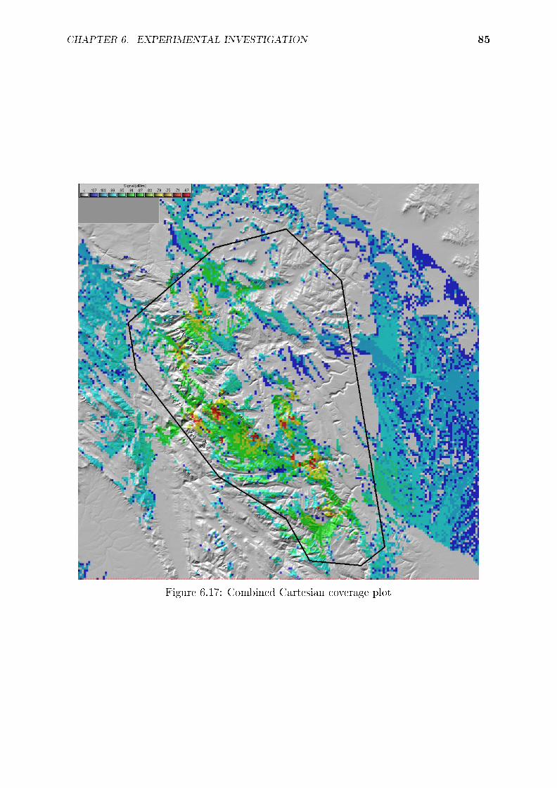
CHAPTER 6. EXPERIMENTAL INVESTIGATION 85
Figure 6.17: Combined Cartesian coverage plot

CHAPTER 6. EXPERIMENTAL INVESTIGATION 86
6.6 Power performance
6.6.1 Motivation
It is necessary to compare the power consumption of all the components given from theirrespective data sheets to actual measured values, so that an accurate power design canbe done. Thereafter a node should be tested for three consecutive days of autonomy inthe case that the sun does not shine and the node will rely entirely on its battery. Thiswill assure reliability.
6.6.2 Experimental setup
In chapter 5 the maximum current draws for each component was given from their respec-tive data sheets. The maximum current that the board will draw in any given situationwill be when the radio is in transmit mode. The maximum power dissipated would be:
Pmax = Pradio−t + PGPS + PuController + P3.3V−regulator + P5V−regulator
= (290× 5) + (36× 5) + (14× 3.3) + (14× (6.5− 3.3)) + (326× (6.5− 5)) = 2, 21WThe total current drawn from the battery will now be measured with a multimeter
with the respective components turned on. For the autonomy test a node is made totransmit a data packet every 10 seconds for 3 consecutive days without a solar panelconnected to charge the battery.
6.6.3 Results
The measured current is 325mA with the battery at 6.5 V. Thus the total maximumpower that the PCB can draw is 2,113W. The node with its 30Ah battery as sized inchapter 5 lasted for three days without completely draining the battery.
6.6.4 Interpretation
The measured power consumption of the components is a bit lower than predicted, whichshould be due to manufacturing variations of components. The node's battery as expectedlasted the three days it was designed for. This shows that the power predictions is notoptimistic and the power source of the system is adequate.
6.7 Summary
The packet error rate test showed that 4800bps is the optimal baud rate for communica-tion. This baud rate is justied since it has 5% packet success over the maximum baudrate of 9600bps. The throughput test showed that the maximum sustainable throughputis achieved at a message arrival rate of 0.1 packets per second (1 packet in 10 seconds).Message arrival rate beyond this number will result in the network becoming congested(unstable). For the current network conguration as in Figure 6.16 the longest path of 6hops will result in an initial route acquisition delay of 12.5 seconds as read from Figure6.10. Range tests in the Cederberg discovered that no non-line-of-sight links are possibleat 151.3MHz, which is in contrast with the Radio Mobile predictions. A maximum reliablelink distance of 10.43km line-of-sight was found. The new predictions from Radio Mobile

CHAPTER 6. EXPERIMENTAL INVESTIGATION 87
using the line-of-sight model yields a study area with just below 50% radio coverage. Thepower test showed that the total predicted power consumption by all components almostequals the measured power consumption, so a power source sized from that predictionsshould be adequate. This was also shown to be adequate by a three day autonomy test.

Chapter 7
Conclusions and recommendations
7.1 Summary and conclusions
This study in ad hoc networks for the application of acquiring wildlife tracking data inthe Cederberg proved to be a viable alternative solution to the current manual techniquesemployed (provided that more than 22 stations are deployed for covering more than 50% ofthe study area). The results in chapter 6 showed a great improvement in time eciencyover the manual techniques used in the past to obtain data. Compared to the severalhours it takes manually, the network will save a lot of a researcher's time. Chapter 1discussed the available solutions for obtaining tracking data over considerable distances.With cost and automation needs in mind, an ad hoc network was deemed to t theproject specications with one unit costing R4048. In chapter 2 the MACAW protocolwas chosen to be most suitable for the data link layer of the communication system andAODV was the chosen protocol for the network layer. These protocols were simulatedin OMNET++ and the results obtained were compared with measured results from thenetwork. The simulation results agreed closely with the measured results. The range testsin the Cederberg yielded somewhat disappointing results compared to the initial RadioMobile prediction. No non-line-of-sight links are possible at 151.3 MHz. The hardwaredesign yielded a functional PCB which were deployed in the eld and showed correctprotocol operation.
7.2 Comparison to prior work
Prior work using ad hoc network architectures for obtaining animal tracking data includesZebranet from [1] and EcoLocate from [19]. Both these networks make use of only mobilenodes (collars) where the network is highly dynamic since animals move around a lot,changing the topology of the network constantly. In this thesis milking stations arenomadic, thus residing at xed locations for extended periods of time. Animal collarsand relaying stations are two distinct designs, where collars only has the task of obtaininglocation information and sending it to milking stations once polled. Milking stations onlyhave the task of obtaining this data and relaying it to a base station. With EcoLocatedierent species of animals are tted with collars to incorporate a broad spectrum ofthe animal kingdom into the network. Zebranet and this work considers only one kindof species, or similar sized animals, whilst this network can be used to relay data fromany type of animal to a base station. EcoLocate ts dierent sized batteries to dierentkind of animals, hence they use a hierarchical approach to routing data in the network,
88

CHAPTER 7. CONCLUSIONS AND RECOMMENDATIONS 89
giving larger animals with larger batteries more trac to route. Mobility inuences thethe routing of packets in EcooLocate. Zebranet uses no routing, all data from collarsis ooded from one collar to the next so that each collar will have information fromevery other collar. This work uses a reactive routing protocol where the routing metricis simply the shortest path to the destination. Solar panels are used by all projects toreplenish a battery which powers collars or relay milking stations. The main dierencebetween this work and the above mentioned is that a dedicated network is used to gatheranimal location information and photos (from collars and camera trap cages) to deliverit to a base station. Whereas Zebranet and EcoLocate gathers only location and sensorinformation from animals and only collars are used to form the network.
7.3 Outstanding issues
The following lists all issues that still needs to be addressed for a reliable network:
A watchdog timer should be implemented to reset each node if something goes wrongand the system does not recover by itself
Nodes should be placed on all positions as predicted with Radio Mobile to conrmthe absolute correctness of the line-of-sight model
A full-edged network should be employed in the Cederberg with leopard collarsand trap cages actively generating trac as a nal network test
7.4 Recommendations for future work
While the network and hardware worked ne, several improvements can be made to makethe system work more eciently. This includes the following:
Incorporate the camera from the leopard trap cage into the milking station designfor immediate transferring of photos to the base station, without a milking stationneeding to poll a camera trap cage for data as with leopard collars.
Change the MACAW protocol to allow for multiple data packets to be downloadedfrom a collar by one POLL packet from a milking station.

Appendices
90

Appendix A
PCB layout
91

APPENDIX A. PCB LAYOUT 92
Figure A.1: PCB top layer
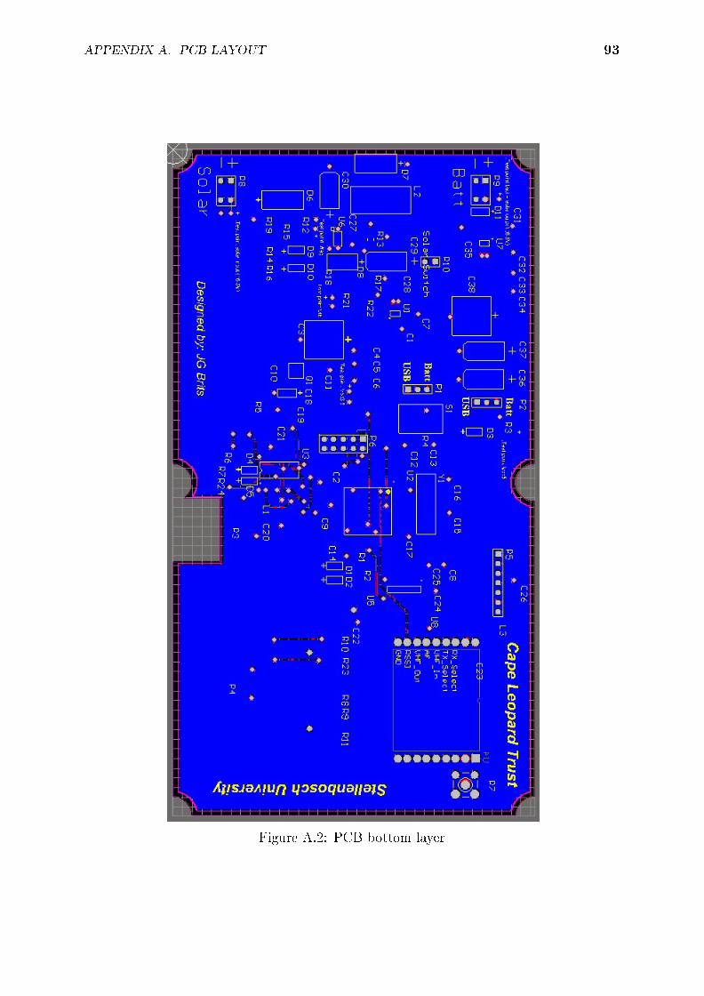
APPENDIX A. PCB LAYOUT 93
Figure A.2: PCB bottom layer
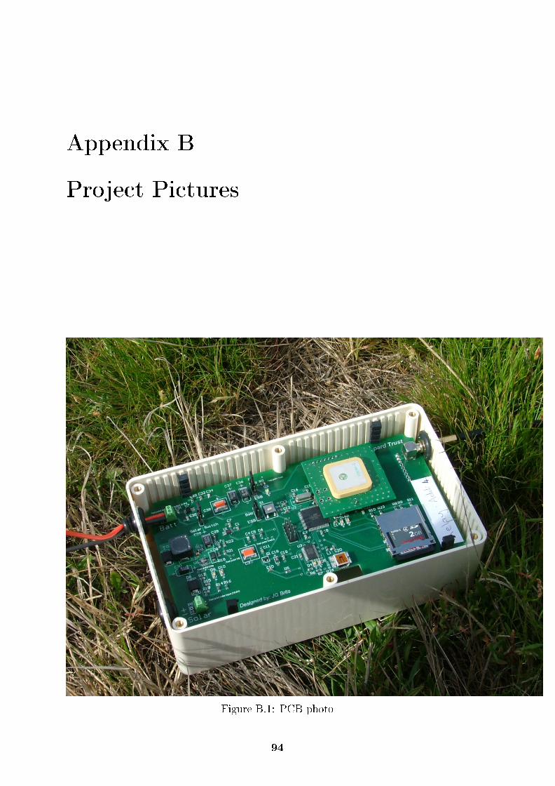
Appendix B
Project Pictures
Figure B.1: PCB photo
94

Bibliography
[1] (2002 November). Engineers and biologists design wireless devices to unlock secrets ofanimal kingdom.Available at: http://www.princeton.edu/pr/pwb/02/1111/1a.shtml, [2009, May 8]
[2] (2004 March). General Notice 533, vol. 465. Department of Communications, GovernmentGazette.
[3] (2006 February). Average temperatures and hours of sunshine in south africa.Available at: http://www.southafricalogue.com/travel-tips/
average-temperatures-and-hours-of-sunshine-in-south-africa.html, [20 October
2009]
[4] (2006 January). Pcb trace width calculator.Available at: http://www.circuitcalculator.com/wordpress/
2006/01/31/pcb-trace-width-calculator/, [2010, February 3]
[5] (2007 November). VHF Narrow Band FM 500mW transceiver. Radiometrix, 1st edn.
[6] (2009). Gps pet tracking devices.Available at: http://www.gps-practice-and-fun.com/gps-pet-tracking.html, [2009,
April 25]
[7] (2009). LT3652: Power Tracking 2A Battery Charger for Solar Power Datasheet. LinearTechnology.
[8] (2009). Satellite tracking.Available at: http://www.seaturtle.org/tracking/faq.shtml, [2009, March 21]
[9] (year unknown). Aerial telemetry.Available at: http://www.skymasters.ca/index.php, [2009, March 12]
[10] (year unknown). Rf link budget calculator.Available at: http://www.afar.net/rf-link-budget-calculator/ , [2009, March 7]
[11] Blake, R. (2001). Wireless Communication Technology. Delmar Thomson Learning.
[12] Chakeres, I.D. and Klein-Berndt, L. (). Aodvjr, aodv simplied. Mobile Computing and
Communications Review, vol. 6, pp. 100101.
[13] Coude, R. (1997). Radio mobile.Available at: http://www.cplus.org/rmw/english1.html, [2009, February 15]
[14] Dobos, M. (2007 June). The osi model.Available at: http://www.tutorial5.com/content/view/26/79/, [2010, November 8]
[15] Foster, R., Ghassemi, M. and Cota, A. (2010). Solar energy - renewable energy and the
environment. CRC Press.
95

BIBLIOGRAPHY 96
[16] Fullmer, C.L. and Garcia-Luna-Aceves, J. (1997). Complete single-channel solutions tohidden terminal problems in wireless lans. IEEE.
[17] Irvine, J. and Harle, D. (2002). Data communications and Networks: an Engineering Ap-
proach. John Wiley and Sons, LTD.
[18] Magna Design Net, I. (2010 September). Review of digital modulation.Available at: http://www.magnadesignnet.com/en/booth/technote/ofdm/page2.php,
[2010, December 10]
[19] Markham, A. (2008). On a Wildlife Tracking and Telemetry System: A Wireless Network
Approach. Ph.D. thesis, University of Cape Town.
[20] Martins, Q. (2010). Why the leopard.Available at: http://www.capeleopard.org.za/, [2010, October 24]
[21] Murthy, C.S.R. and Manoj, B. (2004). Ad Hoc Wireless Networks: Architectures and Pro-
tocols. Prentice hall.
[22] of Science, M.U. and Technology (2008). Microstrip impedance calculator.Available at: http://emclab.mst.edu/pcbtlc2/microstrip.html, [2010, March 13]
[23] Ott, H.W. (2001). Partitioning and layout of a mixed signal pcb. Printed Circuit Design,vol. June.
[24] Paramananthan, S. (1997 November). Error performance of bim transceiver with rs232interface. Tech. Rep..Available at: http://www.radiometrix.co.uk/apps/apnt101.htm
[25] Sande, E. (2010). Kenya: Gsm radio tracking canopies the wildlife. News from Africa.
[26] Sheng, J. (2008). Performance modeling of IEEE 802.11 ad hoc networks under time-varying
channel. Ph.D. thesis, Rensselaer Polytechnic Institute, United States New York.
[27] Tanenbaum, A.S. (2003). Computer Networks:. Pearson Education International.
[28] Warren, H.S. (2003). Hacker's delight. Addison-Wesley.
[29] Wikipedia, t.f.e. (2009 December). Dierential manchester encoding.Available at: http://en.wikipedia.org/wiki/Differential_Manchester_encoding,
[2010, June 7]
[30] Wikipedia, t.f.e. (2010 November). Throughput.Available at: http://en.wikipedia.org/wiki/Throughput, [2010, December 8]
[31] Zyren, J. and Petrick, A. (1998 June). Tutorial on basic link budget analysis. ApplicationNote 9804.