DESIGN OF A VEHICLE BARRIER A THESIS …etd.lib.metu.edu.tr/upload/12616218/index.pdf · DESIGN OF...
113
DESIGN OF A VEHICLE BARRIER A THESIS SUBMITTED TO THE GRADUATE SCHOOL OF NATURAL AND APPLIED SCIENCES OF MIDDLE EAST TECHNICAL UNIVERSITY BY ENGİN METİN KAPLAN IN PARTIAL FULFILLMENT OF THE REQUIREMENTS FOR THE DEGREE OF MASTER OF SCIENCE IN MECHANICAL ENGINEERING SEPTEMBER 2013
Transcript of DESIGN OF A VEHICLE BARRIER A THESIS …etd.lib.metu.edu.tr/upload/12616218/index.pdf · DESIGN OF...
DESIGN OF A VEHICLE BARRIER
A THESIS SUBMITTED TO
THE GRADUATE SCHOOL OF NATURAL AND APPLIED SCIENCES
OF
MIDDLE EAST TECHNICAL UNIVERSITY
BY
ENGİN METİN KAPLAN
IN PARTIAL FULFILLMENT OF THE REQUIREMENTS
FOR
THE DEGREE OF MASTER OF SCIENCE
IN
MECHANICAL ENGINEERING
SEPTEMBER 2013

Approval of the thesis:
DESIGN OF A VEHICLE BARRIER
submitted by ENGİN METİN KAPLAN in partial fulfillment of the requirements for the
degree of Master of Science in Mechanical Engineering Department, Middle East
Technical University by,
Prof. Dr. Canan ÖZGEN __________________
Dean, Graduate School of Natural and Applied Sciences
Prof. Dr. Suha ORAL __________________
Head of Department, Mechanical Engineering
Prof. Dr. Süha ORAL __________________
Supervisor, Mechanical Engineering Dept., METU
Assc. Dr. Serkan DAĞ __________________
Co-Supervisor, Mechanical Engineering Dept., METU
Examining Committee Members:
Prof. Dr. Bülent DOYUM __________________
Mechanical Engineering Dept., METU
Prof. Dr. Süha ORAL __________________
Mechanical Engineering Dept., METU
Prof. Dr. Haluk DARENDELİLER __________________
Mechanical Engineering Dept., METU
Assc. Dr. Serkan DAĞ __________________
Mechanical Engineering Dept., METU
Assc. Dr. Uğur POLAT __________________
Civil Engineering Dept., METU
Date: __________________

iv
I hereby declare that all information in this document has been obtained and presented
in accordance with academic rules and ethical conduct. I also declare that, as required
by these rules and conduct, I have fully cited and referenced all material and results
that are not original to this work.
Name, Last name : Engin Metin KAPLAN
Signature :
v
ABSTRACT
DESIGN OF A VEHICLE BARRIER
Kaplan, Engin Metin
M.S. Department of Mechanical Engineering
Supervisor: Prof. Dr. Süha Oral
Co-Supervisor: Assc. Prof. Dr. Serkan DAĞ
September 2013, 95 pages
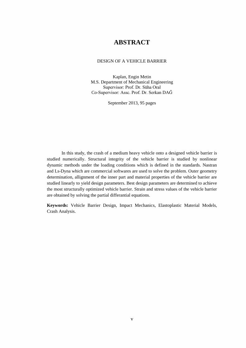
In this study, the crash of a medium heavy vehicle onto a designed vehicle barrier is
studied numerically. Structural integrity of the vehicle barrier is studied by nonlinear
dynamic methods under the loading conditions which is defined in the standards. Nastran
and Ls-Dyna which are commercial softwares are used to solve the problem. Outer geometry
determination, allignment of the inner part and material properties of the vehicle barrier are
studied linearly to yield design parameters. Best design parameters are determined to achieve
the most structurally optimized vehicle barrier. Strain and stress values of the vehicle barrier
are obtained by solving the partial differantial equations.
Keywords: Vehicle Barrier Design, Impact Mechanics, Elastoplastic Material Models,
Crash Analysis.

vi
ÖZ
ARAÇ BARİYERİ TASARIMI
Kaplan, Engin Metin
Yüksek Lisans, Makine Mühendisliği Bölümü
Tez yöneticisi: Prof. Dr. Süha Oral
Ortak tez yöneticisi: Doç. Dr. Serkan DAĞ
Eylül 2013, 95 sayfa
Bu çalışmada, tasarlanan bir araç bariyeri modeline orta boyutlu bir kamyon
tarafından çarpma durumu incelenmiştir. Araç bariyerinin yapısal bütünlüğü, standartlarda
belirtilen yükleme koşulları altında, doğrusal olmayan dinamik metodlarla kontrol edilmiştir.
Çözümlemelerde ticari hesaplamalı katı mekaniği yazılımları Nastran ve Ls-Dyna
kullanılmıştır. Tasarım çalışmaları adına dış geometri hesaplamaları, değişik iç yerleşim
denemeleri ve malzeme özellikleri doğrusal olarak incelenmiştir. Karşılaştırılan
yerleşimlerden en iyisi seçilip yapısal olarak daha dayanıklı bir bariyer modeli oluşturulmaya
çalışılmıştır. Tasarlanan araç bariyerin standartta belirtilen yük altında, üzerinde oluşan
gerinim ve gerilme değerleri ise parçalı diferansiyel denklemler çözülerek görülmüştür.
Anahtar kelimeler: Araç Bariyeri Tasarımı, Çarpma Mekaniği, Elastoplastik Malzeme
Modelleri, Çarpma Analizi.

vii
To My Parents

viii
ACKNOWLEDGEMENTS
I would like to express my appreciation to my supervisor Prof. Dr. Süha ORAL for
his helpful criticism, guidance and patience in the progress and preparation of this thesis.
I want to express my gratitude to my mother Fehamet KAPLAN, my father Dursun
KAPLAN, and my elder brother Ali Murat KAPLAN for their implicit, explicit, and
complimentary help and support not only during my thesis preparation, but also throughout
my life.
I am especially grateful to my wife Sinem KAPLAN for her endless support during
my studies.
ix
TABLE OF CONTENTS
ABSTRACT ............................................................................................................................. v
ÖZ ........................................................................................................................................... vi
ACKNOWLEDGEMENTS .................................................................................................. viii
TABLE OF CONTENTS ........................................................................................................ ix
LIST OF TABLES .................................................................................................................. xi
LIST OF FIGURES ............................................................................................................... xii
LIST OF ABBREVIATIONS ............................................................................................... xiv
LIST OF SYMBOLS ............................................................................................................. xv
CHAPTERS
1. INTRODUCTION ............................................................................................................... 1
1.1 General information ................................................................................................. 1
1.2 Scope of the thesis ................................................................................................... 2
1.3 Literature Survey ..................................................................................................... 3
2. DESIGN CONSIDERATIONS & SOLUTION APPROACHES ....................................... 9
2.1 System Constraints ................................................................................................... 9
2.2 Design Parameters ................................................................................................. 10
2.3 Other Parameters .................................................................................................... 24
2.4 Assumptions ........................................................................................................... 27
3. FINITE ELEMENT MODEL & SOLUTION OF EQUATIONS OF MOTION .............. 31
3.1 Pre-Processing ........................................................................................................ 32
3.1.1 Mathematical Model ...................................................................................... 32
3.1.2 Initial and Boundary Condition ...................................................................... 40
3.2 Solver Execution .................................................................................................... 41
3.2.1 Governing Equations...................................................................................... 41
3.2.2 Other equations .............................................................................................. 45
3.2.3 Input Parameters ............................................................................................ 47
3.2.4 Finite Element Analysis Control .................................................................... 48
4. RESULTS .......................................................................................................................... 49
4.1 PC Properties & Analysis Evaluation .................................................................... 49
4.2 Stress-Strain Results for the Barrier ....................................................................... 56
4.3 Energy Results of the System ................................................................................ 72

x
5. DISCUSSION & CONCLUSION ...................................................................................... 75
5.1 Summary and Comments on the Results ................................................................ 75
5.2 Penetration Limit of the Vehicle Barrier ................................................................ 79
5.3 Structural Integrity Limit of the Vehicle Barrier .................................................... 79
5.4 Future Work ........................................................................................................... 79
REFERENCES ....................................................................................................................... 81
APPENDICES
A. FEM KEYWORD for ALIGNMENT DETERMINATION ............................................. 85
B. CAD Model of the VEHICLE BARRIER ......................................................................... 89
C. PROPERTY of the PC ....................................................................................................... 95

xi
LIST OF TABLES
TABLES
Table 1. Properties of different sized vehicles [16] ................................................................. 9
Table 2. Penetration limitations for different vehicle velocities .............................................. 9
Table 3. Vehicle dimensions .................................................................................................. 11
Table 4. Mechanical properties of the vehicle barrier materials [22], [23] ............................ 13
Table 5. Inertial properties of different cross sectioned ribs .................................................. 14
Table 6. Different rib configuration of the design regions ..................................................... 17
Table 7. Max. v. Misses stress values of the different alignments of the upper side ............. 19
Table 8. Max. v. Misses stress values of the different alignments of the lower side ............. 22
Table 9. Properties of the AISI 304L (m, c, ρ) [30] ............................................................... 29
Table 10. Machanical propterites of the vehicle barrier parts used in analyses [13], [14] ..... 47
Table 11. Machanical propterites of the vehicle parts used in analyses [34] ......................... 47
Table 12. Computer Properties .............................................................................................. 95

xii
LIST OF FIGURES
FIGURES
Figure 1. Vehicle barrier types[2] ............................................................................................ 1
Figure 2. Comparison of the deformed shape of the vehicles [12], [13], [14], [15] ................. 5
Figure 3. Comparison of the acceleration and velocity of the results[12], [13], [15] .............. 6
Figure 4. Comparison of the energy changes of the results[12], [13], [15] .............................. 7
Figure 5. Vehicle barrier example [17] .................................................................................. 10
Figure 6. Ford F800 medium duty truck [18] ......................................................................... 11
Figure 7. Vehicle barrier outer dimensions ............................................................................ 12
Figure 8. Ductile-brittle transition temperature [20] .............................................................. 13
Figure 9. Coordinate system for the ribs ................................................................................ 14
Figure 10. Vehicle barrier parts .............................................................................................. 14
Figure 11. Rib cross sections of the vehicle barrier ............................................................... 15
Figure 12. Side view of the vehicle barrier design regions .................................................... 16
Figure 13. Isometric view of the vehicle barrier design regions ............................................ 17
Figure 14. Linear FEM of the upper side of the vehicle barrier for alignment determination 18
Figure 15. Linear FEM of the lower side of the vehicle barrier for alignment determination 18
Figure 16.Upper side FEA results of the con. A for alignment determination ....................... 19
Figure 17. Upper side FEA results of the con. B for alignment determination ...................... 20
Figure 18. Upper side FEA results of the con. C for alignment determination ...................... 20
Figure 19. Upper side FEA results of the con. D for alignment determination ...................... 21
Figure 20. Upper side FEA results of the con. E for alignment determination ...................... 21
Figure 21. Lower side FEA results of the con. A for alignment determination ..................... 22
Figure 22. Lower side FEA results of the con. B for alignment determination ..................... 22
Figure 23. Lower side FEA results of the con. C for alignment determination ..................... 23
Figure 24. Lower side FEA results of the con. D for alignment determination ..................... 23
Figure 25. Lower side FEA results of the con. E for alignment determination ...................... 24
Figure 26. Joints of the vehicle barrier ................................................................................... 25
Figure 27. Lock mechanism of the vehicle barrier ................................................................. 26
Figure 28. Geometry of the vehicle barrier ............................................................................ 26
Figure 29. Temperature vs. yield stress and ultimate tensile stress for carbon and alloy steels
[27] ......................................................................................................................................... 27
Figure 30. FEM of the vehicle frame ..................................................................................... 33
Figure 31. FEM of the vehicle bed ......................................................................................... 34
Figure 32. FEM of the vehicle cabin ...................................................................................... 34
Figure 33. FEM of the vehicle engine system ........................................................................ 35
Figure 34.FEM of the vehicle drive shaft ............................................................................... 35
Figure 35. FEM of the vehicle front suspension system ........................................................ 36
Figure 36. FEM of the vehicle front axle ............................................................................... 36
Figure 37. FEM of the vehicle front wheel ............................................................................ 37
Figure 38. FEM of the vehicle rear suspension and axle ....................................................... 37
Figure 39. FEM of the vehicle rear wheel .............................................................................. 38
Figure 40.FEM of the vehicle [34] ......................................................................................... 38
Figure 41. FEM of the U, I and Square profile ribs of the vehicle barrier ............................. 39

xiii
Figure 42. FEM of the vehicle barrier .................................................................................... 39
Figure 43. FEM of the ground ............................................................................................... 40
Figure 44. Initial and boundary cınditions of the problem ..................................................... 41
Figure 45. Hourglass modes of the one point integration element ........................................ 45
Figure 46. Force vs Displacement relationship of the nonlinear spring [34] ......................... 48
Figure 47. Time step size vs. time during the execution ........................................................ 49
Figure 48. Deformed shape of the finite element results of the system in different time
intervals .................................................................................................................................. 50
Figure 49. Deformed shape of the finite element results of the barrier in different time
intervals .................................................................................................................................. 54
Figure 50. Crash view of the system in different aspects at time = 0.25 s. ............................ 55
Figure 51. Displacement between leading edge of the vehicle with the attack face of the
barrier vs. time graph ............................................................................................................. 55
Figure 52. Velocity of the vehicle vs. time graph during the crash in x axis(It is taken from
the added cargo mass of the vehicle) ..................................................................................... 56
Figure 53. von Misses stress results of the lower side of the vehicle barrier in different time
intervals .................................................................................................................................. 61
Figure 54. von Misses stress results of the upper side of the vehicle barrier in different time
intervals .................................................................................................................................. 66
Figure 55. von Misses stress results of the plate of the upper side in different time intervals71
Figure 56. Effective plastic strain distrubution in the plate ................................................... 71
Figure 57. Maximum von Misses stress distribution in the joint pins ................................... 72
Figure 58. Energy balance versus time graph during the analysis ......................................... 72
Figure 59. Total, hourglass energy amounts versus time graph during the analysis .............. 73
Figure 60. Spring and damper energy graph .......................................................................... 73
Figure 61. Damping energy of the system vs. time graph ..................................................... 74
Figure 62. Energy ratio vs. time graph................................................................................... 74
Figure 63. Averaged maximum von Misses stress of the element ......................................... 76
Figure 64. Deceleration calculation of the vehicle................................................................. 77
Figure 65. Velocity vs time graph taken from different parts of the vehicle ......................... 78
Figure 66. Penetration limit of the vehicle barrier ................................................................. 93
Figure 67. Structural integrity limit of the vehicle barrier ..................................................... 93
Figure 68. 3D Drawings of the vehicle barrier ...................................................................... 93
xiv
LIST OF ABBREVIATIONS
1D : One-dimensional
2D : Two-dimensional
3D : Three-dimensional
C : Small passenger car
CAD : Computer aided design
FEA : Finite element analysis
FEM : Finite element method
DF : Design Force
DOF : Degree of freedom
: Gravitional Force level
H : Heavy goods vehicle
KPH : Kilometer per hour
M : Medium duty truck
MPH : Mile per hour
MPS : Meter per second
P : Pick-up truck bed
PC : Personal computer
v.M. : Von Misses stress
vs : Versus

xv
LIST OF SYMBOLS
Basic Latin letters:
: Area
: Acceleration value
: Nodal acceleration vector
: Average acceleration at t
: Strain-displacement matrix
: Body load vector
: Fastest wave velocity of material
: Cowper and Symonds strain rate coefficient
: Specific heat
: Displacement boundary condition
: Modulus of elasticity
: Global energy
: External force acting to element
: Internal force acting to element
: Body force density
g : Gravitional force (9.81 m/s2)
: Area moment of inertia
: Stiffness matrix
: Load value
: Mass matrix
: Mass value
: Interpolation matrix
: Unit outward normal to a boundary element
: Pressure

xvi
: Cowper and Symonds strain rate exponent
: Thermal Energy
: Frictional Energy
: Bulk viscosity
: Deviatoric stress
: Temperature value
: Time variable
: Average displacement variable at t
: Average displacement at t+
: Relative volume
: Initial velocity
: Average velocity variable at t
: Average velocity variable at t+
: Velocity value
Xa : Cartesian coordinate before deformation
Xi : Cartesian coordinate after deformation
: Displacement value
: First derivative of the displacement
: Second derivative of the displacement
: Second derivative of the displacement
: Nodal coordinate of the jth node in the ith direction.
: thickness

xvii
Greek letters:
: Time step size
: Time variableat at t+
: Boundary condition at x
: Kronecker delta
: Equilibrium equations
: Strain value
: Plastic strain at failure
: Strain rate
: Strain rate tensor
: Number of first nodal point defining the element
: Number of second nodal point defining the element
: Interpolation function of the parametric coordinates
: Friction coefficient
σ : Stress vector
σYield : Yield Strength
σUltimate : Ultimate tensile strength
: Stability factor
: Stress scale factor for strain rate
υ : Poisson ratio
ρ : Density of the material
: Shear stress value
: Number of third nodal point defining the element

xviii

1
CHAPTER 1
INTRODUCTION
1.1 General information
Vehicle barriers are used as means of defense against any threat in open or closed areas to
provide high security. There are several types of the vehicle barriers shown in Figure 1.
Active barriers can be activated, either by personal, equipment, or both, to permit entry of a
vehicle. Active barrier systems involve barricades, bollards, crash ribs, gates, and active tire
shredders. On the other hand, passive barrier has no movable part. Passive barrier
effectiveness is measured by its capability to absorb impact energy and transmit it to its
foundation. Highway medians, bollards, tires, guardrails, ditches, and reinforced fences are
example of passive barriers. [1]
Figure 1. Vehicle barrier types[2]
High security barrier systems may be kept in the ground or may be over the ground. Several
design criteria must be considered in the design of a vehicle barrier. Furthermore, barrier is
needed to provide qualifications, that are defined in military standards. These standards
indicate the final position of the vehicle after the crash.
Impact mechanic problems should be considered as shock problem rather than static problem
since they are actualized over a short time. In static states the energy applied to the structure

2
is converted into strain, heat and sound energy. On the other hand, the collusion events do
not provide enough time for strain to occur [3]. Deceleration at crash is seen to reach 30 g.
levels in some studies. Different materials can act in completely different in impact when
compared to static loading conditions. Ductile materials like steel tend to become
more brittle at high strain rates [4]. In addition to that, changes in the internal energy in the
material can increase the temperature in impact problems. This must be evaluated, if it can
cause difference in calculations. The calculations may be performed numerically and
analytically.
Material model must include the following properties
Material plasticity
Strain rate effects
Material failure
Temperature effect (If necessary)
1.2 Scope of the thesis
In order to design a vehicle barrier with satisfactory performance under the effect of crash of
a medium heavy truck, one requires the knowledge of impact mechanics and the
implementation techniques of nonlinear dynamic finite element method. Then, by using this
knowledge, appropriate element types, initial and boundary conditions can be determined.
In this thesis, crash of a medium heavy vehicle onto a designed vehicle barrier will be
studied numerically. Studies carried out in this thesis are outlined below:
In Chapter 2, the design options are discussed for the vehicle barrier. Also system constraints
are given for the success of the vehicle barrier.
Finite element model and solution of equation of motion this study are given in Chapter 3.
The pre-processing of the vehicle, vehicle barrier and the ground models are performed.
Element types, connections of the parts, material properties are determined in this chapter.
Explicit nonlinear dynamic solution of the partial differential equation is also given in this
chapter.
In Chapter 4, the numerical studies are presented. Velocity, acceleration and displacement
results of the vehicle and vehicle barrier are displayed here. In addition to that, stress, elastic-
plastic strains and the material failures are evaluated. Energy conversions and the amount of
the energies during the crash are given in this chapter.
Finally, discussions and conclusions about the findings in this thesis are indicated and future
works which can be performed are mentioned in Chapter 5.

3
1.3 Literature Survey
In order to solve the problem of equation of motion, structural element type, elastoplastic
material model, initial and boundary conditions, damping coefficient, friction coefficients
and contact type of the system must be clarified. Various studies are available for the
solution.
Several researchers have worked on crash of the vehicles to the barriers. Eric A. Nelson and
Li Hong study curved barrier impact of a nascar series cars both experimentally and
numerically. Nascar, at the velocity of 135.6 mps, impacts to the barrier with an angle of 25
degree. Both nascar and barrier are modelled and investigated. Post processing is performed
with explicit Ls-Dyna code. It is seen that the curved type barrier is more effective on
deceleration of the cars than flat type barrier. Also, they compare the deceleration results of
the numerical model and test results. Deceleration levels of the numerical results and test
results are in a good agreement [5].
Joseph Hassan et all study on impacting of a car to two different barrier type: deformable
and rigid barrier. They use explicit Ls-Dyna code to solve the nonlinear dynamic equations.
Stress results and wave propagation which is calculated in terms of stress, deformation
pattern and plastic strain energy of the front rail of the vehicle is different in two different
types of the solutions. On the other hand, it is seen that the final deformed shape of the
vehicles are quite similar in numerical and experimental results [6].
Abdullatif K. Zaouk and Dhafer Marzaugui compare the stress results and deformed shape
results of the numerical and test results of the moveable deformable barrier’s side impact
effect study. Solution of the equation of motion is performed with explicit Ls-Dyna finite
element code. They validate finite element results with the test results. Deformed shape of
the car is captured by high speed camera in test. The deformation results of the test seem in a
good agreement with the finite element solution. Acceleration data, which is validated with
the test results. Besides that, they collect force data from a load cell which is located in the
moveable barrier. The results of force data in test setup are quite similar with the numerical
results [7].
M. Asadi et all represent a new finite element simulation model for moving deformable
barrier side impact analysis with explicit Ls-Dyna code. They also perform impact test to
validate their result. A car on which a load cell is mounted hits two different barriers: flat
pole and offset pole with a velocity of 35 kmph. The material properties of the finite element
model are experimentally obtained with compression tests. Final comparison of the general
results shows a strong correlation between test data and numeric results for both the Flat
Wall and Offset Pole tests [8].
Z. Ren and M. Vasenjak studied on crash analysis of the road safety barrier. They develop a
full-sale numerical model of the road safety barrier for use in crash simulations and to further
compare it with the real crash test data. Finite element model of the car and barrier is
prepared by beam and shell elements. Connections of the parts of the vehicle are constraint
with spot welds. Moreover, spring and damper elements are used to simplify calculations.

4
The dynamic nonlinear elasto-plastic analysis is performed with the explicit finite element
Ls-Dyna code. A car, weighing 900 kg has initial velocity of 100 kmph impacted to a barrier
with an angle of 20o
with respect to velocity vector. Car and barrier materials are bilinear
elasto-plastic material model with kinematic hardening and failure criteria. They used
effective plastic strain failure criteria and set the value to 0.28 which corresponds to 28%
ductility. Automatic contact option is defined for parts. Friction coefficients for static and
dynamic cases are taken as 0.1 and 0.05 respectively. According to EN 1317 standard,
impact severity which is a measure of impact consequences for the vehicle is defined by
acceleration severity index [9]. They compare the finite element results of acceleration
severity index with the test results. Comparison of computational and experimental results
proved the correctness of the computational model [10]. M. Borovinsek et all developed Z.
Ren and M. Vasenjak’s study. They prepare finite element models of a bus weighing 13 ton
and a truck weighing 16 ton and impacted them to the barrier with an angle of 20o
with
respect to velocity vector. They also performed test setup of numerical model. Comparison
of the computer simulation and a broad scale experiment demonstrated good correlation of
computational and experimental results for both crash tests [11].
National Crash Analysis Center performs crash tests to different vehicles. They put several
accelerometers on the vehicle and collect data from them. They also prepare finite element
model and solve the differential equations by using explicit Ls-Dyna code. They used rigid
barrier and deformable vehicle models. The vehicle crash to the rigid barrier with a velocity
of 35 kmph and an angle of 20o with respect to
velocity vector. The finite element model of
the vehicles includes shell, rib, solid, spring and damper elements. The deformed shape of
the vehicles, Chevy Silverado [12], C 1500 Pick-up [13], Dodge Neon [14] and Toyota Rav
4 [15] are given in Figure 2.

5
Figure 2. Comparison of the deformed shape of the vehicles [12], [13], [14], [15]
Deformed shape of the finite element solution results are validated by crash tests as shown in
Figure 26. Furthermore, acceleration and velocity data collecting from the left seat of the
vehicles are compared with the numerical results. The results for Chevy Silverado [12], C
1500 Pick-up [13] and Toyota Rav 4 [15] are given in Figure 3.

6
Figure 3. Comparison of the acceleration and velocity of the results[12], [13], [15]

7
It is obvious that, velocity graphs of the vehicles demonstrate the reliability of the numerical
studies. Acceleration data taken from the vehicle are generally close to numerical results.
Besides that, energy balances which is obtained by numerical results also supports that
results are reasonable. They are given in Figure 4.
Figure 4. Comparison of the energy changes of the results[12], [13], [15]

8

9
CHAPTER 2
DESIGN CONSIDERATIONS & SOLUTION APPROACHES
2.1 System Constraints
During the design period of a vehicle barrier, system constraints are needed to be defined.
System constraints are defined in standards, that are independent from the designers.
There is a necessity to address a wide spectrum of a possible incident states such as credible
threat vehicle types for the locale, impact energies and velocities of the various vehicle and
different acceptable penetration limitations. Test standards for security barriers are defined
by ASTM In that standard, the test vehicle was defined as a medium-sized vehicle weighing
6.8 tonnes. According to those weights different penetration limits are allowed for different
crash velocities and kinetic energies. Required velocity and energy ranges are stated. Those
are displayed in Table 1 and Table 2 below.
Table 1. Properties of different sized vehicles [16]
Test Vehicle
(Kg)
Minimum Test
Velocity (km/h)
Permissable
Speed Range
(km/h)
Kinetic Energy
(kJ)
Condition
Designation
Small Passenger
Car (C) (1100)
65 60.1-75 179 C40
80 75.1-90 271 C50
100 90.1-above 424 C60
Pickup truck (P)
(2300)
65 60.1-75 375 PU40
80 75.1-90 568 PU50 100 90.1-above 887 PU60
Medium Duty
truck (M)
(6800)
50 45-60 656 M30
65 60.1-75 1110 M40
80 75.1-above 1680 M50
Heavy Goods
Vehicle (H)
(29500)
50 45-60 2850 H30
65 60.1-75 4910 H40
80 75.1-above 7280 H50
Table 2. Penetration limitations for different vehicle velocities
Required Velocities, kmph
(mph)
Maximum penetration
Limits, m (ft)
50(30) 1(3)
65(40) 6(20)
80(50) 15(50)

10
Real vehicle velocities should be within permissible ranges stated to get the condition
designation. The measured vehicle penetration to the vehicle barrier at the required crash
velocity determines the dynamic penetration state for the condition designation. Penetrations
are referenced to the base of the forward corner of the passenger compartment on the small
passenger car (C), the front leading lower edge of the pickup truck bed (P), the leading lower
edge of the cargo bed on the medium duty truck (M) and the leading lower vertical edge of
the cargo bed on the long heavy goods vehicle (H) [16]. Penetration limits are measured
form the attack face of the barrier.
2.2 Design Parameters
The vehicle, that is used in the calculations, is a Ford F800. The properties of the vehicle are
appropriate for the design consideration as bolded in Table 1. Once system constraints are
defined, design parameters are to be studied for an active barrier. These parameters are listed
below.
Height and width of the barrier
Material selection
Geometry of the ribs
Alignment of the ribs
Height and Width of the Barrier
Vehicle barrier systems can be considered in two different parts. Upper side of the barrier is
the interface between vehicle impact face and the ground. It is located above the ground and
can be penetrate under ground. Lower side is located under the ground. It transfers the
kinetic energy from the upper side of the barrier to the ground. The vehicle barrier example
is given in Figure 5.
Figure 5. Vehicle barrier example [17]

11
Typical systems are investigated. Most of the systems have at least 4 m. width and 1 m.
height (The dimension which is above the ground). Also the embedded part(lower side) is at
least 1 m. hdepth. Dimensions are compared with the vehicle. Dimensions of the medium
duty truck (Ford F800) are given in Table 3. It can be seen that the dimensions for the
vehicle barrier are reasonable according to vehicle.
Figure 6. Ford F800 medium duty truck [18]
Table 3. Vehicle dimensions
Height (m) Width (m) Length (m) Weight (Tonne)
3.5 2.5 8.5 6.8
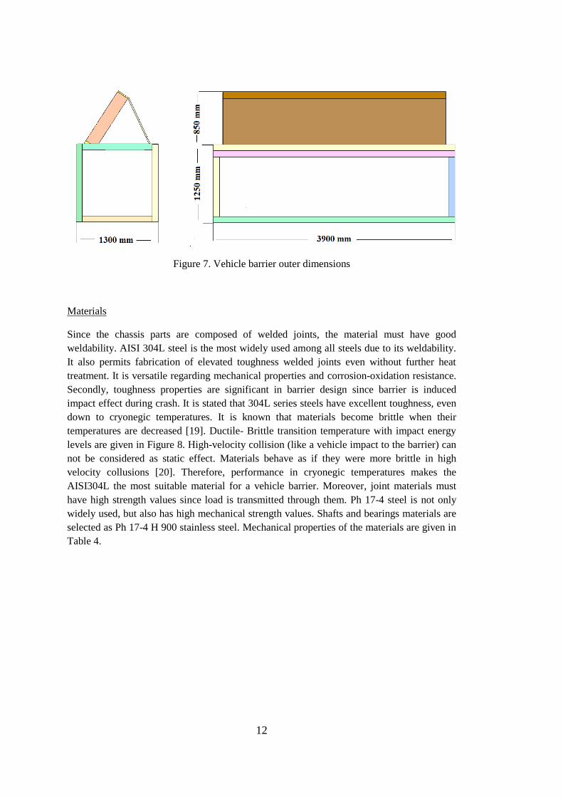
The dimensions for the perimeter of the barriers are given in Figure 7. It can be understood
that dimensions of the barrier are adequate for the vehicle since width of the barrier is longer
than the vehicle.
12
Figure 7. Vehicle barrier outer dimensions
Materials
Since the chassis parts are composed of welded joints, the material must have good
weldability. AISI 304L steel is the most widely used among all steels due to its weldability.
It also permits fabrication of elevated toughness welded joints even without further heat
treatment. It is versatile regarding mechanical properties and corrosion-oxidation resistance.
Secondly, toughness properties are significant in barrier design since barrier is induced
impact effect during crash. It is stated that 304L series steels have excellent toughness, even
down to cryonegic temperatures. It is known that materials become brittle when their
temperatures are decreased [19]. Ductile- Brittle transition temperature with impact energy
levels are given in Figure 8. High-velocity collision (like a vehicle impact to the barrier) can
not be considered as static effect. Materials behave as if they were more brittle in high
velocity collusions [20]. Therefore, performance in cryonegic temperatures makes the
AISI304L the most suitable material for a vehicle barrier. Moreover, joint materials must
have high strength values since load is transmitted through them. Ph 17-4 steel is not only
widely used, but also has high mechanical strength values. Shafts and bearings materials are
selected as Ph 17-4 H 900 stainless steel. Mechanical properties of the materials are given in
Table 4.

13
Figure 8. Ductile-brittle transition temperature [20]
Table 4. Mechanical properties of the vehicle barrier materials [22], [23]
Part Material E(GPa) υ ρ(g/cm3) σYield(MPa)
Ribs and Plates AISI 304L 210 0.3 7.8 515
Joints Ph 17-4 H 900 205 0.3 7.8 1345
Geometry of the ribs
Cross sections of the ribs are determined in this section. It is well known that deflection of
different cross sectioned parts can be different, even when they weigh equal. The deflection
and the stress are given in fixed support–centre loads are given below for elementary beam
theory [24].
Inertial properties about x axes should be maximized in selection of the rib. Coordinate
system for the ribs is presented in Figure 9. I ribs have the highest inertia in equally
weighing structures. The inertial properties of equally weighing structures are given in Table
5. [25].

14
Figure 9. Coordinate system for the ribs
Table 5. Inertial properties of different cross sectioned ribs
Cross Section Type Mass per unit length(g/cm) Area moment of inertia (mm4)
I 757 778000
Square Profile 722 254000
Rectangular 722 333000
Tubular 784 304000
Some parts of the vehicle barrier should have four flat sizes. I rib is not suitable for those
cases. Therefore, square profiles are chosen. They are used in faces of the periphery of the
barrier.
The barrier can be divided in two parts as lower side and upper side as mentioned above. The
geometry is provided in Figure 10.
Figure 10. Vehicle barrier parts
Square profile dimension is determined as 100 mm for the lower side. Once it is selected,
interface profile measurements must be dependent on that dimension. Long length of the I
rib must be selected as 100 mm, since this rib is connected to square rib. Moreover, U rib is
also dependant to this dimension as well. Square profile rib with 100 mm cross section is

15
also used for the upper side of the barrier. In addition to that, U and I rib cross sections must
be greater than lower side, since upper side is directly subjected to the vehicle. Longer side
of the cross section of the U rib is selected as 200 mm. Thus, I rib dimension is determined
since it is connected to interface of the U rib. The upper side and lower side rib dimensions
are given in Figure 11.
Figure 11. Rib cross sections of the vehicle barrier
Since the vehicle is in contact with the upper side of the barrier, a plate must be added at the
top of the I ribs of the upper side. Moreover, two triangular plates are designed between
square rib and I rib at two corners in upper side. Thickness of the plates is considered as 20
mm.
Alignment of ribs in the chassis
Rib alignment in the chassis is significant due to obtained desired strength of the chassis.
Different alignments are studied.
Payload is critical in alignment decision analyses of the chassis. Static analysis is performed
to decide the alignment. It is mentioned that most of the crash events like a truck hitting to
the barrier with a velocity of 50 mph occur between 0.07 and 0.12 seconds [26]. Also, the
design force is significant in the decision of the alignment. Deceleration rate is commonly
used to calculate the design force. The fundamental equation for the design force can be
obtained via Newton’s second law.

16
It is mentioned that the mass of the vehicle is approximately 6800 kg. In spite of the broad
changes in data and experimental techniques, it is possible to understand that a truck
impacting a barrier would have a lower-limit deceleration in the range of 16 to 22g. The
maximum deceleration value is in the range of 62 to 100g. On the other hand, this peak
deceleration rate happens in a very short time (0.01 second). The average deceleration rate
value is in the range of 24 to 31g. This average deceleration value is reasonable and can be
used [15]. The design force can be calculated as
The force is applied to the structure from the approximate contact point.
The analyses are performed via a commercial finite element method code Msc. Nastran. The
Element types are chosen as 1D rib element with I, U and square profile cross sections. The
alignments try-outs and design regions of the barrier are given in Figure 12 and Figure 13.
Upper and lower sides of the vehicle barrier are investigated separately as shown. The
number of upper side ribs is calculated one less than number of lower side ribs since the
length of the upper side is shorter than the length of lower side. There are two perpendicular
and front faces. Same alignment is performed in mutual faces.
Figure 12. Side view of the vehicle barrier design regions

17
Figure 13. Isometric view of the vehicle barrier design regions
Table 6. Different rib configuration of the design regions
Barrier Alignment Region Number of Ribs
A B C D E
Attack Face of Upper Side 5 6 7 8 9
Back Face of Upper Side 5 6 7 8 9
Front Face of Lower Side 6 7 8 9 10
Perpendicular Face of Lower Side 1 1 2 3 4
Bottom Face of Lower Side 6 7 8 9 10
Same alignment try outs are analysed coupled. Barrier is divided into upper and lower side in
the analysis. 1D rib and 2D shell elements are used for modelling the ribs and plates.
Loading is applied from the attack face of the upper side. Static loading is applied to the
structure as a designed force.

18
Figure 14. Linear FEM of the upper side of the vehicle barrier for alignment determination
Beam and shell elements are used for ribs and plates as shown in Figure 10. DOF of the
bottom beams are constrained since their motion is blocked by joint and lower side of the
vehicle barrier. Load is applied from a node which is connected to the beams with nodal
bodies in all directions.
Figure 15. Linear FEM of the lower side of the vehicle barrier for alignment determination
Beam elements are used for ribs as shown in Figure 15. DOF of the bottom ribs are
constrained, since their displacement is block by ground. Load is applied from a node which
is connected to the beams with nodal bodies in all directions.

19
Upper Side of the Barrier Alignment Try Outs
Configuration A to E results is given in Figure 16 to Figure 20. Plates results are not given
since their stress levels are low compared to rib results. As that can be seen from the figures,
stress results are below the yield strength of the AISI 304L. Moreover, it is obvious that
more ribs reduce the stress levels. Configuration C is suitable for the alignment. It is the first
configuration at which the stress level is less than 400 MPa. Maximum von Misses stresses
for the different configurations of the upper side of the barrier are given in Table 7.
Table 7. Max. v. Misses stress values of the different alignments of the upper side
Configuration Max. v.M. Stress(MPa)
A 434
B 416
C 383
D 353
E 338
Configuration A
Figure 16.Upper side FEA results of the con. A for alignment determination

20
Configuration B
Figure 17. Upper side FEA results of the con. B for alignment determination
Configuration C
Figure 18. Upper side FEA results of the con. C for alignment determination

21
Configuration D
Figure 19. Upper side FEA results of the con. D for alignment determination
Configuration E
Figure 20. Upper side FEA results of the con. E for alignment determination
Lower Side of the Barrier Alignment Try Outs
Configuration A to E results are given in Figure 21 to Figure 25. As it can be understood
from the figures, stress results are below the yield strength of the AISI 304L. Furthermore, it
can be seen that usage of more ribs reduce the stress levels. Configuration C is suitable for
the alignment. Stress level drops crucially in the transition of seven to eight ribs. The
maximum von Misses stresses of the different configurations of the lower side of the barrier
are given in Table 8.

22
Table 8. Max. v. Misses stress values of the different alignments of the lower side
Configuration Max. v.M. Stress(MPa)
A 430
B 379
C 244
D 240
E 221
Configuration A
Figure 21. Lower side FEA results of the con. A for alignment determination
Configuration B
Figure 22. Lower side FEA results of the con. B for alignment determination

23
Configuration C
Figure 23. Lower side FEA results of the con. C for alignment determination
Configuration D
Figure 24. Lower side FEA results of the con. D for alignment determination

24
Configuration E
Figure 25. Lower side FEA results of the con. E for alignment determination
Preprocess of the FEM rib model keyword for the alignment determination is given in
Appendix A.
2.3 Other Parameters
There are other parameters ,needed in design. They are given below;
Joint type and design
Lock mechanism of the upper side to lower side
Joint type and design
Revolute joint, located between lower side and upper side of the barrier must allow upper
side, to penetrate into the lower side. It is determined to use two joints. The diameter of the
joint can be calculated by considering the design force. Half of the designed force must be
considered since two shafts are presented.
Shear stress, that is induced because of the designed force, can be calculated by using area of
the structure.

25
Shear stress can be converted to von misses stress by using distortion energy theory as it is
given by equation (2.5).
√
The yield stress of the joint material of the Ph 17-4 H 900 is 1345 MPa. as shown in Table 4.
Shear stress limit of the joint for the safe design can be calculated as given below.
√
Shear stress of the shaft must be greater than 776.5 MPa. Then, the area of the shaft can be
calculated.
√
The diameter of the shaft must be greater than 20 mm. It is set as 20 mm. Also, the shear
area of the bearing must be greater than 1215 mm2. Since the outer diameter and inner
diameter is chosen as 50 mm. and 20 mm. respectively, it is considered as safe design. Joints
and bearings are shown Figure 26.
Figure 26. Joints of the vehicle barrier

26
As it is seen in Figure 22 the ribs next to bearings are chosen U rib, since it has longer flat
area than square ribs.
Lock mechanism of the upper side to lower side
Vehicle barrier must include a lock mechanism to transform energy from the upper side to
lower side when it is subjected to crash. Top ribs of the front face of the lower side (number
1) constraints the bottom rib of the upper face (number 2) to raise as shown in Figure 27.
Figure 27. Lock mechanism of the vehicle barrier
The final geometry of the vehicle barrier is shown in Figure 28.
Figure 28. Geometry of the vehicle barrier

27
Details of the model are given in Appendix B.
2.4 Assumptions
Material stiffness may decerase as the temperature increases. Thus, strength of the material
may change. Temperature increase due to friction between impacting objects in the crash
problems. The change of the yield and ultimate tensile stress values of carbon and alloy
steels are given in Figure 29.
Figure 29. Temperature vs. yield stress and ultimate tensile stress for carbon and alloy steels
[27]

28
The elementary frictional interactions consist of the transient touching of two parts. As the
parts slide past each other, work is performed by the friction energy, which transforms to the
thermal energy [28]. The frictional energy and frictional load can be calculated as they are
given in equation (2.7) and (2.8).
∫
Here L is load, V means velocity and corresponds to the average deceleration rate of
the vehicle which is taken as 27 g. before. Mass of the vehicle is 6800 kg. Velocity of the
vehicle is 80 kmph which yields 22.2 mps. Static maximum friction coefficient is taken 0.8
in applications to have conservative solution. [29].
Crash scenario is supposed to be ended in maximum 0.15 seconds. Therefore integration
limits are zero and 0.15 seconds.
∫
The interaction faces of the vehicle and barrier is approximately 1 m2. As it is mentioned
before, there is a plate in the attack face of the barrier which has a 20 mm. thickness. It is
assumed that heat energy which transformed from the friction energy, transferred only and
no work interactions exist across its boundary. The energy balance can be written as, given
by, equation (2.9), where Q is the amount of net heat transfer to the system [30].
Here m is total mass and c means specific heat for the material. T1 and T2 are temperature
values.
In order to have a conservative solution, the quarter mass of the interaction face of the plate
is taken. Thus, the front part of the plate is assumed to have greater temperature value. Mass
and specific heat of the plate are given in Table 8.
29
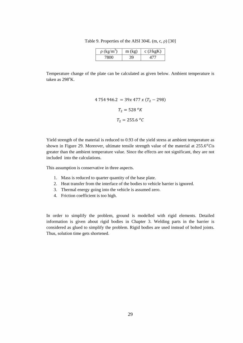
Table 9. Properties of the AISI 304L (m, c, ρ) [30]
ρ (kg/m3) m (kg) c (J/kgK)
7800 39 477
Temperature change of the plate can be calculated as given below. Ambient temperature is
taken as 298oK.
Yield strength of the material is reduced to 0.93 of the yield stress at ambient temperature as
shown in Figure 29. Moreover, ultimate tensile strength value of the material at 255.6 is
greater than the ambient temperature value. Since the effects are not significant, they are not
included into the calculations.
This assumption is conservative in three aspects.
1. Mass is reduced to quarter quantity of the base plate.
2. Heat transfer from the interface of the bodies to vehicle barrier is ignored.
3. Thermal energy going into the vehicle is assumed zero.
4. Friction coefficient is too high.
In order to simplify the problem, ground is modelled with rigid elements. Detailed
information is given about rigid bodies in Chapter 3. Welding parts in the barrier is
considered as glued to simplify the problem. Rigid bodies are used instead of bolted joints.
Thus, solution time gets shortened.

30

31
CHAPTER 3
FINITE ELEMENT MODEL & SOLUTION OF EQUATIONS
OF MOTION
Finite element method is a numerical method to solve partial differential equations with
some approximations [31]. In implicit method, average displacements can be evaluated as
{ } [ ] { }
Here u represents displacement, K is stiffness matrix and F is the external force. It is
acceptable for linear problems. On the other hand contact, geometry and material plastic
behavior makes the problem nonlinear. Convergence problem can be seen in nonlinear
implicit cases.
In explicit cases, central difference method is used and accelerations are evaluated at time t
as
{ } [ ] ([ ] [[
]])
Here a represents acceleration, M is mass matrix, Fext is the external force and Fint is the
internal force. .As it is seen in the equation the inverse of the mass matrix is multiplied by
the difference between external and internal forces. The velocities and displacements are
then calculated [32].
{ } { } { } (3.3)
{ } { } { } (3.4)
Explicit finite element method is more appropriate for dynamic impact mechanic problems.
In numerical calculations, three main stages must be conducted.
1) Pre-Processing
2) Solver Execution
3) Post-Processing

32
Pre-Processing is the stage where the elements, nodes, initial and boundary conditions are
identified. Modeling objectives are defined and computational grid is created. In the second
stage numerical models are set to start up the solver. In the implicit calculations, solver runs
until the convergence is acquired. On the other, in the explicit calculations, solution
execution is finished when the defined time limit is reached. Furthermore, the duration of the
time depends on the time step size which is formulated below.
√
Here is stability factor which is a constant value. L is the smallest element length for one
dimensional element. Average length formulations are used in two or three dimensional
elements. C is wave velocity of the material. For an isotropic material C is root square of
stiffness to density ratio [33].
Results are evaluated in post-processing stage.
3.1 Pre-Processing
In this study, the aim is to investigate the structural integrity of the vehicle barrier under an
impulsive effect of the vehicle by explicit time integration method. Therefore, an equivalent
numerical model is needed to be created.
3.1.1 Mathematical Model
Multiple parts of the vehicle body can be modeled as plates. Therefore plate-like structures
are considered to simplify the solution. Four-node fully integrated elements are used due to
its calculations are quicker than others. In addition to that, some chassis parts of the vehicle
are modeled by beams. Hughes-Liu beam is used in calculations [33]. Other structural solid
type elements are defined and calculated in the form of fully integrated eight-node
hexahedral solid elements. Welded connections of the different parts are connected each
other with spot weld. In addition to that shear and normal forces for the failure of the welds
are defined. In welded connections, all six DOFs of welded nodes are calculated equally.
Tires are modeled with shell elements and connected to the vehicle with revolute joints.
Pressure is applied to the interior element faces to simulate tire air pressure. It is not
necessary to model detailed parts of the vehicle such as driver, engine and suspension
system. Mass equivalent models are built for engine, clutch and transmission. Point element
mass model is performed for driver. Equivalent discrete spring and damper model are
created for suspensions. Additional mass of the cargo and radiators are also modeled.
Bolted connections in the vehicle are not modeled since it is computationally time
consuming. Nodal rigid bodies are used instead of the bolts.

33
Vehicle, barrier and ground parts can be classified in eleven groups:
Vehicle frame
Vehicle Bed
Vehicle cabin
Vehicle engine system
Vehicle drive shaft
Vehicle front suspension
Vehicle front axle
Vehicle rear suspension and axle
Vehicle rear wheel
Vehicle barrier
Ground
Vehicle Frame
Frame is constructed with side and cross members, rear bumpers, suspension mounts, rear
suspension brackets, vertical posts, stiffeners, tank brackets, front bumper supports and
clutch bearings. Elements are created by three or four node shell elements. Parts are
connected to each other with spot-weld. The parts of the frame are given in Figure 30.
Figure 30. FEM of the vehicle frame
34
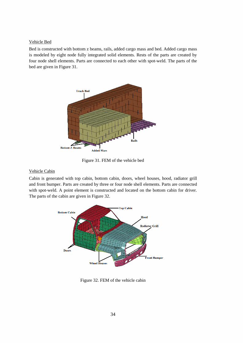
Vehicle Bed
Bed is constructed with bottom z beams, rails, added cargo mass and bed. Added cargo mass
is modeled by eight node fully integrated solid elements. Rests of the parts are created by
four node shell elements. Parts are connected to each other with spot-weld. The parts of the
bed are given in Figure 31.
Figure 31. FEM of the vehicle bed
Vehicle Cabin
Cabin is generated with top cabin, bottom cabin, doors, wheel houses, hood, radiator grill
and front bumper. Parts are created by three or four node shell elements. Parts are connected
with spot-weld. A point element is constructed and located on the bottom cabin for driver.
The parts of the cabin are given in Figure 32.
Figure 32. FEM of the vehicle cabin

35
Vehicle Engine System
Engine system is modeled with transmission, clutch, front-middle and back radiators, and
grill. Grill is created by three or four node shell elements. Rests of the parts are modeled by
eight node fully integrated solid elements. Parts are connected to each other by nodal rigid
bodies in six degree of freedom. The parts of the engine system are given below.
Figure 33. FEM of the vehicle engine system
Vehicle Drive Shaft
Drive shaft system is modeled with rear axle, front-rear drive shafts universal joints, and
carrier bearings. Parts are created by three or four node shell elements. Universal joints are
connected to each other by spherical joints. Other parts are connected with nodal rigid
bodies. The parts of the drive shaft are given in Figure 34.
Figure 34.FEM of the vehicle drive shaft

36
Vehicle Front Suspension
Front suspension model is created with shock absorbing dampers and housings, front axle,
bracket mounts, spring fixtures, suspension springs, suspension leaf springs, and suspension
brackets. Parts are created by three or four node shell elements. Parts are connected with
nodal rigid bodies. The parts of the front suspension are given in Figure 35.
Figure 35. FEM of the vehicle front suspension system
Vehicle Front Axle
Front Axle model is created with wheel hubs, brake disks, front axle, center link and mounts.
Parts are created by three or four node shell elements. Parts are connected with nodal rigid
bodies. The parts of the front suspension are given in Figure 36.
Figure 36. FEM of the vehicle front axle

37
Vehicle Front Wheel
Front wheel model is created with front wheels, front axle and center link. Parts are created
by three or four node shell elements. Parts are connected with nodal rigid bodies. The parts
of the front wheel are given in Figure 37.
Figure 37. FEM of the vehicle front wheel
Vehicle Rear Suspension and Axel
Rear Suspension model is created with rear axle, rear suspension springs and suspension leaf
springs. Parts are created by three or four node shell elements. Parts are connected with
nodal rigid bodies. The parts of the rear suspension are given in Figure 38.
Figure 38. FEM of the vehicle rear suspension and axle
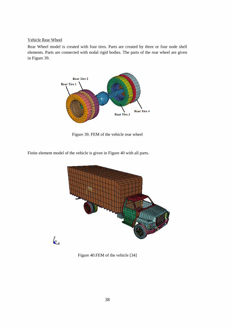
38
Vehicle Rear Wheel
Rear Wheel model is created with four tires. Parts are created by three or four node shell
elements. Parts are connected with nodal rigid bodies. The parts of the rear wheel are given
in Figure 39.
Figure 39. FEM of the vehicle rear wheel
Finite element model of the vehicle is given in Figure 40 with all parts.
Figure 40.FEM of the vehicle [34]

39
Barrier model
Solid model is constructed according to design parameters. The eight-node solid elements
with fully integrated is used in solid elements. Welded parts are connected to each other with
bonding contact type. Failure can be observed by defining the shear and normal force
components for the contacts. The lock mechanism and revolute joints are also modeled. The
elements of the U, I and square profile ribs are given in Figure 41.
Figure 41. FEM of the U, I and Square profile ribs of the vehicle barrier
Finite element model of the vehicle barrier is given in Figure 42.
Figure 42. FEM of the vehicle barrier

40
Ground model
Ground model is created by rigid elements. Vehicle barrier is embedded into ground model.
Elements of the surface on which the vehicle is driven are created as four node shell
elements. Elements of the ground in which the barrier is embedded are modeled as eight
node solid elements. The images of the ground model are given in Figure 43.
Figure 43. FEM of the ground
3.1.2 Initial and Boundary Condition
Since the ground is supposed to be fixed, all displacement DOF of the ground and ground
barrier housing model are constraint. Thus, vehicle barrier’s degrees of freedom are
constraint by positive contact of its ground housing model. Vehicle barrier is connected to
the ground from the bottom side with bolted joints. Instead of that, nodes at the bottom face
of the vehicle barriers’ displacements are constraint in all directions.
The vehicle is initially moved at 50 kmph in x direction through the barrier. Gravitational
force is given for all parts in negative z direction as 9.81 m/s2. Initial and boundary
conditions are given in Figure 44.

41
Figure 44. Initial and boundary cınditions of the problem
3.2 Solver Execution
3.2.1 Governing Equations
As it is mentioned before, time-dependent deformation is considered in explicit method.
Assuming a point in a body, located at a (Xa) in a fixed cartesian coordinate system moves to
a point at i (Xi). The deformation can be calculated in terms of the coordinates (Xa) and time
t, due to a Lagrangian formulation is considered.
At t = 0, the initial conditions can be expressed. means initial velocity.
Solution of the momentum equation is sought in the equation below.

42
Traction boundary condition must be satisfied.
On boundary displacement boundary conditions
Discontinuity of the contact on boundary becomes
(
)
Along an interior boundary when
. represents cauchy stress, is the
density, f is the body force density, means acceleration, the comma denotes covariant
differentiation, and is a unit outward normal to a boundary element of
Mass conservation is provided
where V is the relative volume and is the mass. The determinant of the displacement
gradient matrix is
The energy equation can be expressed as it is seen below.

43
It is integrated in time domain and is used not only for equation of state calculations, but also
for a global energy balance. In Equation (2.12) and p are the deviatoric stress and
pressure.
Here, q represents bulk viscosity, is the Kronecker delta ( = 1 if i = j; otherwise = 0)
and is the strain rate tensor.
It can be written:
∫( ) ∫ ( ) ∫ (
)
where satisfy all boundary conditions on . Also, integrations are over the geometry.
Divergence theorem yields
∫( ) ∫ ∫ (
)
In addition to that, having knew that
( )
It yields to the form of the equilibrium equations,
∫ ∫ ∫ ∫

44
It can be superimposed a mesh of finite elements interconnected at nodal grids on a reference
configuration and follow nodes through time,
∑
represents interpolation function of the parametric coordinates k is the number
of nodal points calling the element, and is the nodal coordinate of the jth node in the ith
direction.
∑
and it can be written
∑ ∫ ∫
∫ ∫
where
Equation (2.21) transforms in matrix notation
∑ {∫ ∫
∫ ∫
}

45
N represents interpolation matrix, is the stress vector.
( )
B is the strain-displacement matrix, a represents the nodal acceleration vector.
{
}
{
}
Body load vector is b and t is the applied traction load [35].
{
} {
}
3.2.2 Other equations
Hourglass Effect
Zero Energy deformations for the one-point integrated solid element can be seen in Figure
45.
Figure 45. Hourglass modes of the one point integration element
There is one integration point in the every face of the cubic element. As it can be seen
integration point does not move at some modes of the element. This mesh distortion

46
produces no strains or volume change due to integration point is not changed. Hourglass
energy must be checked. The amount of the hourglass energy cannot exceed ten percent of a
hundred of the total energy [36].
Material Properties
Piecewise plastic and plastic kinematic material properties are used for vehicle and barrier
respectively. Elasto-plastic formulation also considers the yield of the material. Furthermore
strain-rate can be also accounted for both material types. It uses Cowper and Symonds
formulation which scales the yield stress with a factor [33].
(
)
Here is the strain rate, p and C are the constants.
Viscous dampers are used for front suspension system. This material provides a linear
translational damper located between two nodes.
Here, F is calculated force and is the velocity of the node.
Nonlinear elastic springs can be defined and accounted for the calculations. It provides
translational and rotational springs with arbitrary force versus displacements.
Constraints
Nodal Constraints makes groups of nodes to move together in one or limited degree of
freedom. Acceleration of the groups can be calculated as it is given below.
∑
∑

47
Here n is the node number and is the acceleration of the jth constraint node in the ith
direction. There are two nodes in the group if the constraint is defined as spot weld [32].
3.2.3 Input Parameters
Mechanical material properties of the vehicle and the vehicle barrier are given in Table 10
and Table 11. Vehicle barrier parts yield strengths are scaled with a factor (0.85) due to
indicate safety factor.
Table 10. Machanical propterites of the vehicle barrier parts used in analyses [13], [14]
Part E(GPa) υ ρ(g/cm3) σy(MPa) f(mm/mm) C
* p
*
Barrier ribs and plates 210 0.3 7.8 440 0.3 40 5
Barrier joints 210 0.3 7.8 1143 0.11 40 5
Table 11. Machanical propterites of the vehicle parts used in analyses [34]
Vehicle Part Behavior E(GPa) υ ρ(g/cm3) σy(MPa) ϵf(mm/mm)
Frame System Elastoplastic 205 0.3 7.85 385 0.4
Bed System Elastoplastic 205 0.3 7.85 155 0.3
Added Mass Elastic 2 0.3 0.03 - -
Cabin System Elastoplastic 205 0.3 7.85 155 0.4
Engine System Rigid 205 0.3 7.85 - -
Suspension System Elastoplastic 205 0.3 7.85 700 0.1
Wheel System Elastic 205 0.3 7.85 - -
Axle System Elastoplastic 205 0.3 7.85 385 0.4
Ground is modeled as rigid elements. Also, motions of the nodes are constrained in six
directions. Because of no motion is calculated for the ground model, the input parameters are
not significant.
Linear Damper and nonlinear spring models are created to simulate suspension system with
one dimensional element. The damping constant is specified as 1 [34]. Force vs.
displacement curve of the nonlinear spring is given in Figure 46.

48
Figure 46. Force vs Displacement relationship of the nonlinear spring [34]
Weld spot failures when the constrained force between two nodes exceeds 50 kN [34].
Damping for the all steel materials is calculated as 0.02. Moreover gravitational force is
accounted as 9.81 m/s2.
3.2.4 Finite Element Analysis Control
Hourglass energy, energy dissipation, damping energy and sliding energy are computed
through the analysis and they are indicated to the energy balance. Moreover displacement,
velocity, acceleration are calculated for rigid and flexible bodies. In addition to that,
principle strains, principle stresses, von Misses stresses and effective plastic strains are
calculated for beam, shell and solid elements. Furthermore, kinetic energy, internal energy,
sliding energy, hourglass energy and total energy are calculated. All results are calculated in
one millisecond time intervals.

49
CHAPTER 4
RESULTS
4.1 PC Properties & Analysis Evaluation
The finite element solution of the mathematical model is performed by computer system.
The memory properties of the system are given at Appendix C.The computational time is
significant in explicit-type finite element analysis. The total analysis takes approximately
0.25 seconds. Furthermore, it takes 150 hours in computer system. The analysis is performed
until the vehicle is spring backed from the vehicle barrier. Actually, velocity of the vehicle in
x direction drops to zero at 0.135 seconds. But, it is important to observe the vehicle after
this time. It is ensured that vehicle has consumed its kinetic energy at the end of the analysis.
The vehicle barrier protects its structural integrity at the end of the numerical calculation. In
addition to that maximum penetration of the the leading lower edge of the vehicle to the
attack face of the barrier is less than 1 m. in analysis. Thus, it can be said that vehicle barrier
is successful according to designation F2656-07 ASTM standard numerically.
Time step size is important in explicit calculations since it affects the analysis duration. Time
step size during the solver execution is given in Figure 47.
Figure 47. Time step size vs. time during the execution
The deformed shape of the vehicle and the barrier is given in Figure 48 by 0.25 s. time
intervals. It can be understood that vehicle crashes and gets back.

50
Figure 48. Deformed shape of the finite element results of the system in different time
intervals

51
The deformed shape of the barrier is given in Figure 49 by 0.25 s. time intervals. It can be
understood that barrier is deformed up to the 0.15 seconds. In addition to that, it recovers
after 0.15 seconds since vehicle consumes its kinetic energy.

52

53

54
Figure 49. Deformed shape of the finite element results of the barrier in different time
intervals
Scenes of the system in different aspects at the end of the analysis are given in Figure 50. It
can be seen that structural integrity of the barrier is protected.

55
Figure 50. Crash view of the system in different aspects at time = 0.25 s.
The penetration of the leading edge of the vehicle with respect to attack face of the vehicle
barrier is given in Figure 51. It can be seen that displacement increases up to 0.135 s. since
vehicle does not lose its kinetic energy. Furthermore it decreases after 0.175 s. since vehicle
spring backs from the barrier. Penetration limit does not exceed 1000 mm as it can be seen in
figure.
Figure 51. Displacement between leading edge of the vehicle with the attack face of the
barrier vs. time graph
The velocity of the vehicle represents its energy during the analysis. It is given in Figure 52.
It can be seen that velocity of the vehicle drops to zero at 0.135 s. Moreover it increases in
negative direction after 0.135 s.

56
Figure 52. Velocity of the vehicle vs. time graph during the crash in x axis(It is taken from
the added cargo mass of the vehicle)
4.2 Stress-Strain Results for the Barrier
Von Misses stress results of the lower side of the vehicle barrier is given in Figure 53 by
0.25 s. time intervals.

57

58

59

60

61
Figure 53. von Misses stress results of the lower side of the vehicle barrier in
different time intervals
Von Misses stress results of the upper side of the vehicle is given in Figure 54 barrier by
0.25 s. time intervals.

62

63

64

65

66
Figure 54. von Misses stress results of the upper side of the vehicle barrier in
different time intervals
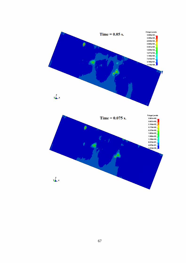
Von Misses stress results of plate of the upper side is given in Figure 55 by 0.25 s. time
intervals.
67

68

69

70
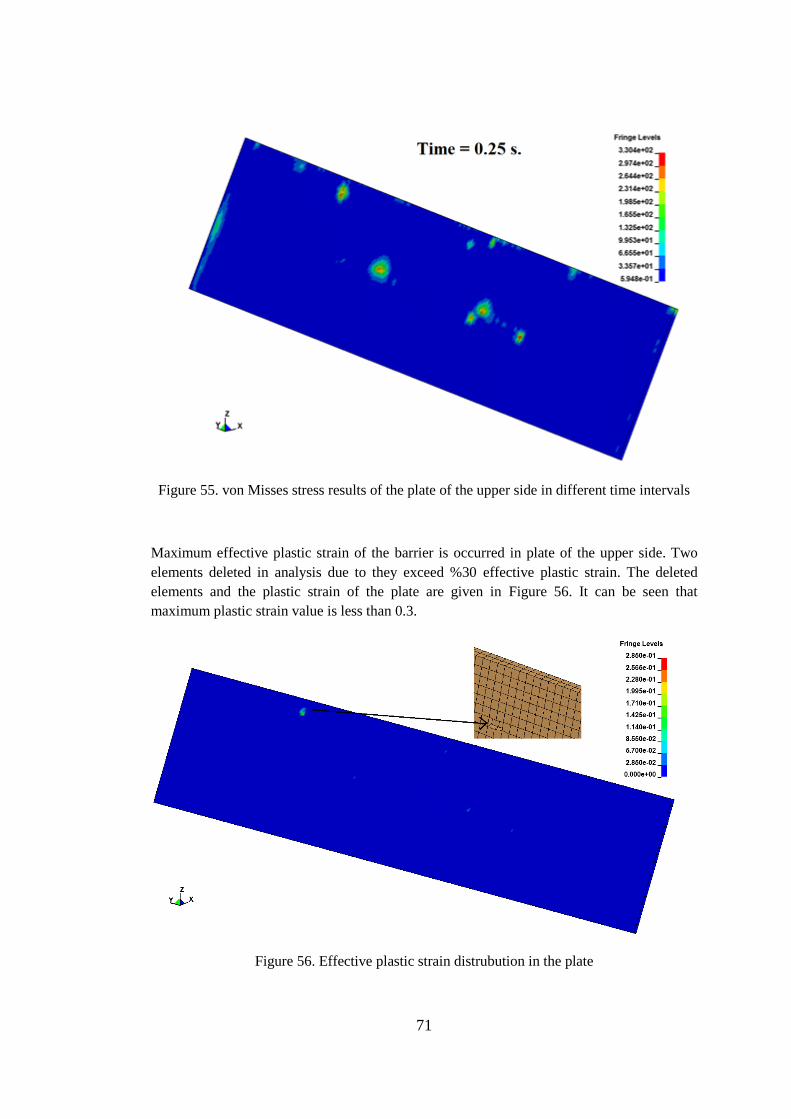
71
Figure 55. von Misses stress results of the plate of the upper side in different time intervals
Maximum effective plastic strain of the barrier is occurred in plate of the upper side. Two
elements deleted in analysis due to they exceed %30 effective plastic strain. The deleted
elements and the plastic strain of the plate are given in Figure 56. It can be seen that
maximum plastic strain value is less than 0.3.
Figure 56. Effective plastic strain distrubution in the plate
72
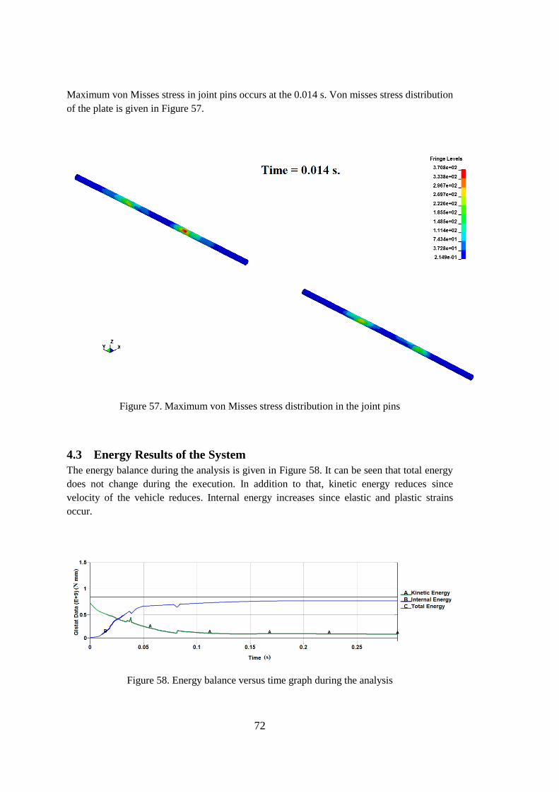
Maximum von Misses stress in joint pins occurs at the 0.014 s. Von misses stress distribution
of the plate is given in Figure 57.
Figure 57. Maximum von Misses stress distribution in the joint pins
4.3 Energy Results of the System
The energy balance during the analysis is given in Figure 58. It can be seen that total energy
does not change during the execution. In addition to that, kinetic energy reduces since
velocity of the vehicle reduces. Internal energy increases since elastic and plastic strains
occur.
Figure 58. Energy balance versus time graph during the analysis

73
Hourglass energy must be maximum %10 of the total energy during the analysis as it is
mentioned before. The total energy and hourglass energy versus time domain is given in
Figure 59. It can be seen that it is %1.75 of the total energy during the analysis.
Figure 59. Total, hourglass energy amounts versus time graph during the analysis
Suspension system is modelled by discrete springs and damper elements as it is mentioned
before. The energy of the discrete elements is given in Figure 60. It can be seen that energy
increases until the velocity of the vehicle is reduced to zero. After that point energy level
decrease since the vehicle gets elevated after the crash.
Figure 60. Spring and damper energy graph
The damping energy of the system with respect to time domain is given in Figure 61. It can
be seen that the slope of the graph decreases since energy of the system reduces.

74
Figure 61. Damping energy of the system vs. time graph
Energy ratio between initial energy and converted energy is displayed in Figure 62. It can be
seen that the ratio is not one during the analysis. It decreases to 0.96 at the end of the
analysis. This is because of the deleted elements and nodes.
Figure 62. Energy ratio vs. time graph

75
CHAPTER 5
DISCUSSION & CONCLUSION
5.1 Summary and Comments on the Results
In this thesis, numerical crash scenario of the vehicle to the barrier with the explicit dynamic
finite element code is studied in order to design and construct a stable vehicle barrier. In this
respect, different design options are considered in order to obtain the highest stiffness to
mass ratio selection. The system model is simulated in computer environment, and solved
numerically with commercial finite element code. For the compensation of the nonlinear
dynamic equations, the central difference method is considered.
In order to reach this level, firstly general information about the numerical calculations of the
systems and their validations via crash tests at the few decades is given. After the high
reliability of these numerical calculations is observed, the design of the vehicle barrier is
introduced. System requirements are investigated to see what qualifications are necessary in
vehicle barriers.
Secondly, selection of the material, outer dimensions of the system, rib selections and
alignments, lock mechanism and joint mechanisms of the vehicle barrier are determined.
Material is significant in two aspects.
Weldability
High strength
Rib selection is important since the vehicle barrier is constructed with several ribs. Square
profile ribs are more appropriate since they have flat faces in the usage of the barrier faces
edges. On the other hand, I beam is the most suitable in usage of the barrier faces. Rib
alignment is important since it directly affects the mass and stiffness of the barrier. In this
respect, different try-outs are performed to see stress levels with commercial finite element
code with a static load which is applicable for crash analysis. Lock mechanism is also
determined for the vehicle barrier since it is under the ground when it is embedded. Also,
joint between upper and lower side of the vehicle barrier is designed. Assumptions, which
make the calculations shorter, but not have important role in the systems, are defined. For
instance, temperature increase due to friction of the vehicle and the vehicle barrier is
ignored. Because, it does not change significantly mechanical properties of the materials.
Finite element model generation of the vehicle, vehicle barrier and ground is necessary for
pre-process. Since the vehicle barrier model is more important here, the elements are chosen
quite small. The plasticity of the materials is determined which may also indicate the
mechanical failure due to plastic strain. Initial and boundary conditions are defined which is
appropriate for the real crash scenario. Later, solution of equation of motion is studied.
Finally, solution of the problem with images and graphs are given at the end of the study.

76
Time step size is a parameter that determine the time of the analysis. Firstly it is started with
0.55e-7 seconds. As the time increases, time step size is reduced as it is seen in Figure 47.
This is because of the element which has the smallest dimension has deleted due to plastic
strain. Another time step drop is seen in 0.035 seconds. This reduction has same reasons.
Numerical calculations is continued with 0.26e-7 second until the analysis is completed.
Maximum von Misses stress at the upper side of the vehicle barrier is locally 450 Mpa at the
0.125 seconds as given in Figure 54. This stress level is high since it is not average stress.
The graphical view represents stress from nodes. Actually averaged von Misses stress level
of the element is about 250 Mpa as given in Figure 63.
Figure 63. Averaged maximum von Misses stress of the element
Maximum plastic strain at that stress level is 0.28. Maximum plastic strain at failure of the
material is specified 0.3 in the literature. Therefore, failure has not happened at that stress
level. In addition to that maximum von Misses stress at the upper side of the vehicle barrier
is locally 475 Mpa. at the 0.05 seconds as given in Figure 53. Average maximum von Misses
stress of the element is about 250 Mpa. The failure is not observed during the analysis in
lower side of the barrier. The maximum von Misses stress of the vehicle barrier parts
exceeds the yield strength of the material. Therefore, permanent plastic strain occurred in the
barrier. It can be seen that the vehicle barrier shape at the end is different from the original
shape as given in Figure 49. But, they do not exceed ultimate tensile strength of the material.
Maximum von Misses stress of the plate is occurred at the 0.075 seconds as given in Figure
55. Two elements failed due to maximum effective plastic strain. Deleted elements are given
in Figure 56.

77
It can be said that the barrier deforms maximum between 0 and 0.075 seconds as it is shown
in Figure 49. This is because of the first impact energy absorption. Deformation and stress
results are reduced after the impact effect as it is given in Figure 53, Figure 54 and Figure
55. The barrier returns the stable with plastic deformation at the end of the analysis.
Deceleration of the vehicle can be calculated by the help of the velocity graph. The total
velocity drop to zero through that time interval gives the acceleration level. It is given in
Figure 64.
Figure 64. Deceleration calculation of the vehicle
The deceleration level is calculated about 10g. It is average value. Local high deceleration
value can be higher than 10g.
It can be said that different parts of the vehicle has alternating deceleration. Velocity graph,
shown in Figure 52 is taken from the added mass of the vehicle. In addition to that, the
velocity drop graph taken from the different parts of the vehicle is given in Figure 65.

78
Figure 65. Velocity vs time graph taken from different parts of the vehicle
It can be said that the velocity drop initially occurs in the lower part of the vehicle. This is
because of the height of the vehicle barrier. Attack face of the barrier firstly blocks the lower
parts of the vehicle. It can be understood that, the curves moves together after 0.1 seconds. It
can be seen from the Figure 48 that, the space between bed and cabin gets minimized and
moves back as the energy of the vehicle drops.
Total energy level is not changed during the analysis as shown in Figure 58. Total energy is
composition of internal energy, kinetic energy, hourglass energy, spring-damper energy and
damping energy. Internal energy of the system increases since the strain energy occurs in the
parts as elastically and plastically. It is normal that kinetic energy drops since vehicle barrier
blocks the motion of the vehicle. The sudden peaks and drops in the internal and kinetic
energy may be cause of the element deletion of the parts. In addition to that, hourglass
energy level is quite low according to total energy as it is shown in Figure 59. Spring and
damper energy increases in negative direction until impact effect is finished. The vehicle is
elevated and probably the deflection of the damper and springs is reduced after that point.
Therefore the energy of the springs and dampers are reduced at the 0.15 seconds as it is
shown in Figure 60. Later, equilibrium is broken and springs and dampers are loaded again.
Damping energy of the system has increasing value. But, the slope of the curve is decreased.
This is because of the kinetic energy of the system is decreased. Initial energy to converted
energy ratio is given in Figure 62. It can be seen that there are sharp drops in the graph. This
is because of the element deletion of the system. The deletion is occurred both from the
vehicle and the vehicle barrier.
In conclusion, vehicle barrier is investigated numerically with different aspects. It can be
said that vehicle barrier is stable to the crash of the medium heavy vehicles as it is proven in
this thesis.

79
5.2 Penetration Limit of the Vehicle Barrier
Penetration limit, which is defined as 1 m. in the standard, is seek according to variable
vehicle velocity. According to analysis, at velocities which is greater than 59 kmph., vehicle
barrier penetration limit exceeds 1m. Deformed shape is given in Figure 66 below.
Figure 666. Penetration limit of the vehicle barrier
5.3 Structural Limit of the Vehicle Barrier
Structural Limit of the vehicle barrier is found. Vehicle barrier cannot protect its structural
integrity at velocity of 85 kmph. The crash view is given in Figure 67.
Figure 677. Structural integrity limit of the vehicle barrier
5.4 Future Work
In this study, a finite element model of the system which is studied numerically and
validated experimentally in [22], [23], [24], [25], [26], [27], [28], [29], [30], [31] and [32] is
generated and solved in the impact effect numerically. The trustworthiness of the numerical
results with the experiments of the literature is enhanced the solution of the problem. In
addition to that an experimental validation can be performed for the numerical results.
Accelerometers, load cells and strain gages with high sampling frequencies can be used in
crash tests. Numerical results can be compared by test result data.

80
81
REFERENCES
[1] Unified Facilities criteria(UFC), “Selection and application of vehicle barriers”,
USA, 1990
[2] U. S. Deparment of Transportation Federal Transit Administration, “ Appendix E
Vehicle Barrier Selection and Implamentation”, Transit Security Design
consideration, Washington DC USA, 2001
[3] Goldsmith, W., “Impact Theory and Physical Behavior of Colliding Solids”, Dover
Publications, 2001
[4] Poursartip, A., “Instrumented Impact Testing at High Velocities”, Journal of
Composites Technology and Research, vol 15 issue 1, 1993
[5] Nelson, E.A., Hong, L., “Curved barrier impact of a nascar series stock car”, 8th
International Ls-Dyna Users Conference, Crash Safety, Altair Engineering
[6] Hassan, J., “Interpretation of deformation pattern in automotive rails in frontal
impact”, 7th International Ls-Dyna Users Conference, Crash Safety, Scientific Labs
and Proving Grounds DaimlerChrysler Corp., USA
[7] Zaouk, A.K., Marzougui, D., “Development and validation of a US side impact
moveable deformable barrier FEM”, FHWA/NHTSA National Crash Analysis
Center, The George Washington University, USA
[8] Asadi, M., Tattersall, P., Walker, B., Shirvani, H., “Advanced Finite Element Model
for AE-MDB Side Impact Barrier”, 6th International Ls-Dyna Users Conference,
[9] European Committee for Standardization, “European Standard EN 1317-1”, EN
1317-2, Road Restraint Systems, 1998.
[10] Ren, Z., Vesenjak, M., “Computational and experimental crash analysis of the road
safety barrier”, University of Maribor, Faculty of Mechanical Engineering,
Slovenia, 2005
[11] Borovins,ˇM., Vesenjak, M., Ulbin, M., Ren, Z., “Simulation of crash tests for high
containment levels of road safety barriers”, University of Maribor, Faculty of
Mechanical Engineering, Slovenia, 2007
[12] FHWA/NHTSA National Crash Analysis Center, “Finite Element Model of Chevy
Silverado”, The George Washington University , Version 2, 2007

82
[13] FHWA/NHTSA National Crash Analysis Center, “Finite Element Model of C1500
Pickup Truck” , The George Washington University, Verison 7,1994
[14] FHWA/NHTSA National Crash Analysis Center, “Finite Element Model of Dodge
Neon”, The George Washington University, Version 7, 1996
[15] FHWA/NHTSA National Crash Analysis Center, “Finite Element Model of Toyota
Rav 4”, The George Washington University, Version 1, 1997
[16] Designation F2656-07, “American Society of Test Materials (ASTM)”, Standard Test
Method for Vehicle Crash Testing of Perimeter Barriers
[17] Avon Barrier Company, “ RB780CR Chieftrain High Security Road Blocker”, Avon
Barrier Catalogues, Bristol England, 2013
[18] Ford Company, “ Ford F800 Truck Properties”, Ford Truck Catalogues, USA, 2000
[19] Goldsmith, W., “Impact; the Theory and Physical Behaviour of Colliding Solids”,
Dover Publications, ISBN 0-486-42004-3, 2001
[20] Sandvik Materials Technology Corparation, “Datasheet of SAF 3207 HD is a
hyper-duplex (austenitic-ferritic) stainless steel”, Seamless tube and pipe According
to ASTM A789/A790, Mc Graw Hill, Pp 37-38, Sweden, January 2012
[21] Shigley, J.E., Mischke C.R., Brown, T.H., “Standard Handbook Machine Design”,
third edition, Mc Graw Hill, Pp 32.12
[22] Material Property Database, “AISI 304L properties”, Jahm Software, Inc., USA,
1998
[23] AK Steel Corporation, 17-4 PH Stainless Steel, “Product Data sheet”, UNS S17400,
2007.
[24] Budynas, R.G., Nisbett J.K., “Shigley’s Mechanical Engineering Design”, eight
edition in si units, Mc Graw Hill, Pp 997, 2008.
[25] Şen İ.Z., Özçilingir, N., “Machine elements data sheet”, Deha publication, pp 117-
118, 123, Istanbul, 2004
[26] Terry, P., Tholen, M., “Vehicle Barrier Design”, Tech Briefs, Determining degrees
of effectiveness, Tech Briefs No:2, Burns Mc-Donnel, 2003
[27] Budynas, R.G., Nisbett J.K., “Shigley’s Mechanical Engineering Design”, eight
edition in si units, Mc Graw Hill, Pp 39-40, 2008

83
[28] Bhushan, B., “Tribology: Friction, Wear, Lubrications”, The Engineering
Handbook, Ed. Richard C. Dorf, Boca Raton: CRC Press LLC, 2000
[29] Engineering Toolbox, “Friction and Coefficients of Friction”, Resources, Tools and
Basic Information for Engineering and Design of Technical Applications, Usa, 2013
[30] Çengel, Y. A., “Heat Transfer”, A practical approach, International edition, pp 38-
949, 2000.
[31] Pelosi, G., "The finite-element method, Part I: R. L. Courant: Historical
Corner". DOI:10.1109/MAP.2007.376627., 2007
[32] Ansys Training Explicit Dynamics with Ansys Ls-Dyna, “Introduction, Ansys Inc.”,
2nd
Edition, Release 11.0, Manual, chapter 1, Inventory 002539 2-8, pp12-14, 2008
[33] Yoo, Y. H., Yang, D. Y., “Finite element modeling of the high-velocity impact
forging process by the explicit time integration method”, Department of Mechanical
Engineering, KAIST, Taejon 305-701, KOREA
[34] Marzougui, D., Mohan, P., Kan, S., “National transportation research center F800
Single Unit Truck FEM Model for Crash Simulations with Ls-Dyna”, George
Washington University
[35] Hallquist, J. O., “Ls-Dyna Theoretical Manual”, Livermore Software Technology
Corporation, pp 21-24, May 1998
[36] Ansys Training Explicit Dynamics with Ansys Ls-Dyna, “Release 11.0”, 2nd
Edition
Manual, chapter 2, elements-hourglassing, Ansys Inc., Inventory 002539 2-8, pp 8-9,
2008
[37] Ansys Training Explicit Dynamics with Ansys Ls-Dyna, “Release 11.0”, 2nd
Edition, Manual, chapter 2, elements-hourglassing, Ansys Inc., Inventory 002539 2-
8, 2008

84

85
APPENDIX A
FEM KEYWORD for ALIGNMENT DETERMINATION
$ NASTRAN input file created by the Patran 2010 64-Bit input file
$ translator on May 07, 2013 at 14:41:47.
$ Direct Text Input for Nastran System Cell Section
$ Direct Text Input for File Management Section
$ Direct Text Input for Executive Control
$ Linear Static Analysis, Database
SOL 101
CEND
$ Direct Text Input for Global Case Control Data
TITLE = MSC.Nastran job created on 24-Apr-13 at 16:27:41
ECHO = NONE
SUBCASE 1
$ Subcase name : Default
SUBTITLE=Default
SPC = 2
LOAD = 2
DISPLACEMENT(SORT1,REAL)=ALL
SPCFORCES(SORT1,REAL)=ALL
STRESS(SORT1,REAL,VONMISES,BILIN)=ALL
BEGIN BULK
$ Direct Text Input for Bulk Data
PARAM POST 0
PARAM PRTMAXIM YES
$ Elements and Element Properties for region : kutu_y
PBEAML 1 1 BOX
100. 100. 5. 5.

86
$ Pset: "kutu_y" will be imported as: "pbeaml.1"
CBEAM 126 1 127 128 1. 0. 0.
CBEAM 127 1 128 129 1. 0. 0.
CBEAM 128 1 129 130 1. 0. 0.
.
.
.
CBEAM 2060 5 2069 1944 1. 0. 0.
$ Referenced Material Records
$ Material Record : steel
$ Description of Material : Date: 22-Apr-13 Time: 23:17:55
MAT1 1 210000. .3 7.8+9
$ Multipoint Constraints of the Entire Model
$ ID conflict : the PATRAN MPC ID was 1
RBE3 2607 2593 123456 1. 123 148 149
150 151 152 153 154 155 156 205
206 207 208 209 210 211 212 262
263 264 265 266 267 268 269 318
319 320 321 322 323 324 325 374
375 376 377 378 379 380 381 431
432 433 434 435 436 437 438 486
487 488 489 490 491 492 493 798
799 800 801 802 803 804 805 806
855 856 857 858 859 860 861 862
863 908 909 910 911 912 913 914
915 916 917 918 919 920 921 962
963 964 965 966 967 968 969 970
971 972 973 974 975 1020 1021 1022
1023 1024 1025 1026 1076 1077 1078 1079
1080 1081 1082 1133 1134 1135 1136 1137

87
1138 1139 1140 1141
$ Nodes of the Entire Model
GRID 1 650. 1950. 1250.
GRID 2 650. 1950. 1240.
GRID 3 650. 1950. 1230.
.
.
.
GRID 2593 0. 0. 1950.
$ Loads for Load Case : Default
SPCADD 2 1
LOAD 2 1. 1. 1
$ Displacement Constraints of Load Set : dofs
SPC1 1 123456 126 648 774 832 888 942
999 1054 1112 1165 1422
SPC1 1 123456 1424 THRU 1812
SPC1 1 123456 1815 THRU 1944
SPC1 1 123456 2072 THRU 2460
SPC1 1 123456 2463 THRU 2591
$ Nodal Forces of Load Set : payload
FORCE 1 2593 0 1.8+6 -1. 0. 0.
$ Referenced Coordinate Frames
ENDDATA b8f7a4f3
$ Elements and Element Properties for region : I_x
PBEAML 3 1 I1
50. 7. 86. 100.

88

89
APPENDIX B
CAD Model of the VEHICLE BARRIER
Figure 68. 3D Drawings of the vehicle barrier(cont’d)

90
Figure 68. 3D Drawings of the vehicle barrier(cont’d)

91
Figure 68. 3D Drawings of the vehicle barrier(cont’d)

92
Figure 68. 3D Drawings of the vehicle barrier(cont’d)

93
Figure 68. 3D Drawings of the vehicle barrier

94

95
APPENDIX C
PROPERTY of the PC
Table 12. Computer Properties
Property Value
Processor Intel (R) Core (TM) i5-3470@ 3.20 GHz
Installed Memory (RAM) 8.00 GB
System Type 64-bit Operating System